model weight output(s) - oregon state...
TRANSCRIPT
1
Modeling for Non-Modelers
Modeling for Non-Modelers
A Gentle Introduction to
Mathematical Models
Modeling for Non-Modelers
What is a Model?
Modeling for Non-Modelers
Input(s) ? Output(s)
Model
A model, at it’s most basic, takes one or more
inputs, and processes those inputs into one
or more outputs
Modeling for Non-Modelers
10
15
20
25
30
35
40
1500 2000 2500 3000 3500 4000 4500 5000
MP
G
Vehicle Weight
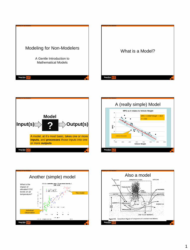
MPG as it relates to Vehicle Weight
Individual Observation
A (really simple) Model
MPG = 0.0084*Weight + 48.8
r2 = 0.82
Modeling for Non-Modelers
Another (simple) model
What is the
impact of
elevated CO2
levels on air
temperature?
Individual
Observation
The model
Modeling for Non-Modelers
Also a model

2
Modeling for Non-Modelers Modeling for Non-Modelers
Causal Loop Diagram of a Model Examining the Growth or Decline of a
Life Insurance Company
Source: Robert A. Taylor, U.S. Department of EnergyC = negative (counteracting) feedback loop, || = delays
Modeling for Non-Modelers
Things to do with models
• Generate new, testable hypotheses
about a system.
• Explore emergent properties of a
system.
• Understand our ignorance.
• Predict the future.
• Perform virtual experiments.
• Optimize decisionmaking about
the system.
Modeling for Non-Modelers
And some downsides…• They can be difficult to understand. This complexity can pose significant
barriers to understanding by end-users.
• Models contain many "hidden" assumptions. Know what these
assumptions are before using the model!!!
.
• The results of model runs
may be believed to easily.
Be a skeptic!
• Models, particularly complex
models, can be expensive
and time consuming to
develop, implement and
validate.
Modeling for Non-Modelers
A Hierarchy of Approaches
Math
em
atical M
odels
Empirical (Statistical – Data-
Driven)
Regression
Linear
Logistic (classification)
NonlinearMachine Learning
Process(Theory-driven)
Analytical Models(closed-form
solution)
Simulation Models (computer-based)
Point (1-D)
Systems Dynamics
Semi-distributed(2/3-D)
Fully Distributed (2/3-D)
Inc
rea
sin
g c
om
ple
xity
/ha
ss
le/p
ow
er
Modeling for Non-Modelers
The Process of Modeling
Real World Mathematical World
Real-world problemRepresent
SystemState assumptions
Identify system,
mathematical
representation,
parameters,
structure (e.g.
equations)
Interpret
solutions/
results with data
Real-world
solutions

3
Modeling for Non-Modelers
Is your model any good?
• You need data – as much as possible
• Partition your data into two
independent sets – one for
calibration, one for
validation
Verify ValidateCalibrate
Modeling for Non-Modelers
Tools• Excel – great for simpler models, regression – a bunch of
built-in tools for simple data analysis, statistical modeling
• R, Python – simple, interpreted
open source (free) programming
languages, rich modeling support
• Visual Tools – Stella, Simile,
PowerSim, GoldSim…
• MatLab – OSU site license,
simple programming, rich math
modeling support
• Traditional Programming Languages – C++, FORTRAN
– powerful, computationally efficient, but more hassle to
work with – often used for large, complex models.
Modeling for Non-Modelers
A Tale of Four Models
Next, we will (briefly) explore four models and
modeling approaches:
1. A simple regression model (in Excel, Python)
2. A classification model (Logistic Regression) in
Python
3. A population model
in Python
4. A systems dynamics
model using Python
Modeling for Non-Modelers
To access the Jupyter Notebooks
• https://bee-jupyter.bee.oregonstate.edu
• User: jupyter2
• Password: robot
Modeling for Non-Modelers
Model 1 – Empirical Model
Goal: Identify relationship between two
variables based on data
This is an example of an ‘empirical’ (or
“statistical”) model:
1) data driven (not physically-based)
2) assume a model form (e.g. Y=aX+b)
3) use regression to find best fit parameters
Modeling for Non-Modelers
Linear Regression - Excel
Dataset available at: http://explorer.bee.oregonstate.edu/Topic/Wodel/Data/StreamTemp.x
lsx
Approach:
1. Load Data into Excel
2. Plot the data of
interest
3. From the plot, add
regression lines
4. Generate summary
statistics
4
Modeling for Non-Modelers
Model 2 - Classification
• Classification models categorize sets of
inputs in two or more discrete bins.
A common example:
predicting species
presence/absence based
on environmental factors
We want to understand
the probability that a given
combination of factors will
result in a “positive” result
Modeling for Non-Modelers
Logistic Regression - Python
• Jupyter Notebook available at: https://bee-
jupyter.bee.oregonstate.edu/user/jupyter2/notebooks/Classificatio
n%20and%20Logistic%20Regression.ipynb
• Approach:
1. Load Data into
Python
2. Take advantage of
pre-existing package
(sklearn) for doing all
the work
Modeling for Non-Modelers
Model 3 – Population DynamicsProblem: Predator-Prey Interactions - The Lotka-
Volterra Equations
The Lotka-Volterra equations were developed in the early part of the 20th century as a simple description of the dynamics of two populations, one predating on the other.
An example might be arctic foxes and arctic hares.
Modeling for Non-Modelers
The MathProblem: Predator-Prey Interactions - The Lotka-Volterra
Equations
This is arguably the simplest possible model of predation. Translating to a
mathematical description results in the following:
• Rate of Change of Prey H = [ growth rate of Prey ] - [ loss due to predation
• Rate of Change of Predator P = - [losses due to mortality ] + [ growth due to
predation ]
bHPPrdt
dP
aHPHrdt
dH
P
H
Questions:
1. Under what circumstances might this model be
reasonable?
2. How do we solve the resulting system of
equations?
3. Under what conditions (if any) are the populations
in equilibrium?
4. Do the equilibrium point imply stability?
Modeling for Non-Modelers
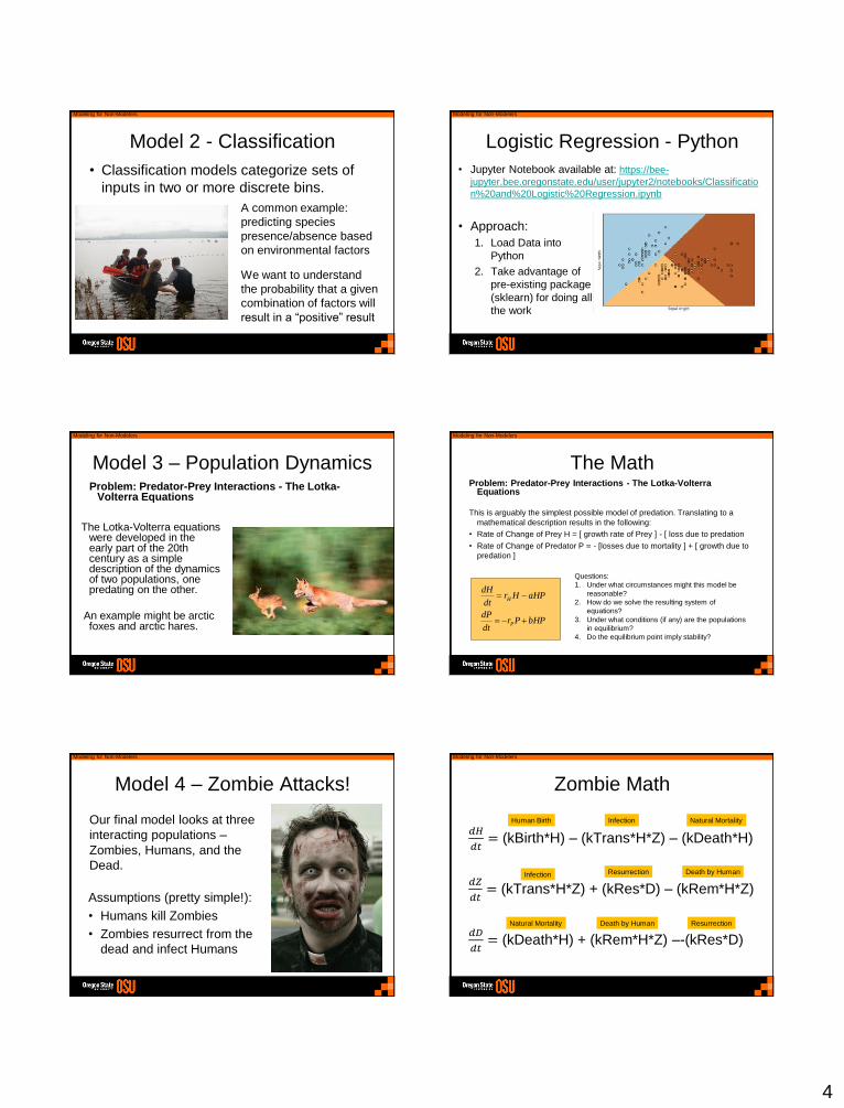
Model 4 – Zombie Attacks!
Our final model looks at three
interacting populations –
Zombies, Humans, and the
Dead.
Assumptions (pretty simple!):
• Humans kill Zombies
• Zombies resurrect from the
dead and infect Humans
Modeling for Non-Modelers
Zombie Math
𝑑𝐻
𝑑𝑡= (kBirth*H) – (kTrans*H*Z) – (kDeath*H)
𝑑𝑍
𝑑𝑡= (kTrans*H*Z) + (kRes*D) – (kRem*H*Z)
𝑑𝐷
𝑑𝑡= (kDeath*H) + (kRem*H*Z) –-(kRes*D)
Human Birth Infection Natural Mortality
Natural Mortality
Infection
Resurrection
Death by Human
Death by Human
Resurrection

5
Modeling for Non-Modelers
Things to think about
• All models are wrong,
some models are useful.
Be sure yours is in the
latter group.
• Keep it as simple as possible,
but not too simple…
• Model iteratively – start
simple, add complexity as needed
• Modeling is a great way to generate insights,
explore and understand the world…
Modeling for Non-Modelers
Extras
Modeling for Non-Modelers
Uses of Models
Three Primary Uses of Models:
• Analysis
• Prediction
• Control
Additional Secondary Uses
include:
• Conceptual framework for organizing or coordinating empirical research
• Mechanism to summarize or synthesize large quantities of data
• Mechanism to identify areas of ignorance
• Gaming - providing insight to managers by performing "what-if" simulations
Modeling for Non-Modelers
A few more benefits...
• Results in a description that is precise and unambiguous – good as a
means of communication.
• Models enable predictions
to be made in such a way
that these predictions can be
checked against reality by
experiment.
• Capture knowledge about a
system in a durable,
distributable form.
• Models can be Fun!
Modeling for Non-Modelers
Additional considerations…
• Realism: the degree to which model structure mimics the real world - how completely does the model capture reality
• Precision: the accuracy of the model predictions - how well does the model generate results?
• Generality: the ability of the model to adequately represent diverse systems - is the model broadly useful?
• Often, these properties trade off against each other.
Modeling for Non-Modelers
An ExampleObjective
• Construct a description of the dynamics of the worlds population such that the time when the population size will double can be computed:
Assumptions (Hypotheses)
• We will model the population as whole, not individuals, ages, sexes,etc.
• The population grows at a constant per capita rate – not influenced by internal or external factors
rteNNrNdt
dN0
where r is the intrinsic per capita growth rate
To calibrate the model, we solve for r
Resulting Model
time N k= 0.1
0 0.01 N0 0.01
1 0.011052
2 0.012214
3 0.013499
4 0.014918
5 0.016487
6 0.018221
7 0.020138
8 0.022255
9 0.024596
10 0.027183
11 0.030042
12 0.033201
13 0.036693
14 0.040552
15 0.044817
16 0.04953
17 0.054739
18 0.060496
20 0.073891
22 0.09025
24 0.110232
26 0.134637
28 0.164446
30 0.2008550
0.05
0.1
0.15
0.2
0.25
0 10 20 30 40
Time
Exponential Growth
6
Modeling for Non-Modelers
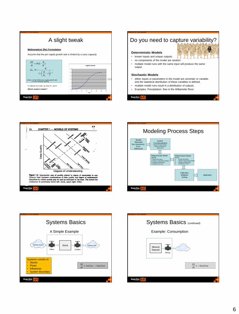
A slight tweak
Mathematical (Re) Formulation
Assume that the per-capita growth rate is limited by a carry capacity
Which model is better?
rteN
K
KNSo
K
NrN
dt
dN
11
,
)1(
0
where r is the intrinsic per capita growth rateK is the carrying capacity
To calibrate the model, we solve for r and K
Modeling for Non-Modelers
Do you need to capture variability?
Deterministic Models
• known inputs and unique outputs.
• no components of the model are random
• multiple model runs with the same input will produce the same
output.
Stochastic Models
• either inputs or parameters in the model are uncertain or variable,
and the statistical distribution of these variables is defined.
• multiple model runs result in a distribution of outputs.
• Examples: Precipitation; flow in the Willamette River.
Modeling for Non-Modelers Modeling for Non-Modelers
Modeling Process Steps
Identify
Rationale/
Key Question(s)
to be
Addressed
System
ConceptualizationAbstract Critical System
Features Relevant to
Question(s):
Diagrammatic ModelIdentify1.System Boundary
2.System Components (States)
3.Linkages (flows/rates)
4.Exogenous drivers
Mathematical ModelIdentify:
1. System Boundary
2. System Components (states)
3. Linkages (flows/rates)4. Exogenous drivers
Calibration
Validation
Testing
Application
Modeling for Non-Modelers
Systems Basics
Stock
Inflow Outflow
Systems consist of:
• Stocks
• Flows
• Influences
• System Boundary
External Source External Sink
A Simple Example
𝑑𝑦
𝑑𝑡= 𝐼𝑛𝑓𝑙𝑜𝑤 − 𝑂𝑢𝑡𝑓𝑙𝑜𝑤
Modeling for Non-Modelers
Systems Basics (continued)
Mineral
DepositMining
Example: Consumption
𝑑𝑦
𝑑𝑡= −𝑂𝑢𝑡𝑓𝑙𝑜𝑤
7
Modeling for Non-Modelers
Systems Basics (continued)
Stock of water in a reservoir
𝑑𝑊
𝑑𝑡= 𝑃𝑟𝑒𝑐𝑖𝑝 + 𝐼𝑛𝑓𝑙𝑜𝑤 − 𝐸𝑣𝑎𝑝𝑜𝑟𝑎𝑡𝑖𝑜𝑛 − 𝐷𝑖𝑠𝑐ℎ𝑎𝑟𝑔𝑒
Precipitation EvaporationWater in
Reservoir
(W)
River Inflow Discharge
Note: A Stock can be
increased by decreasing it’s
outflows, as well as
increasing it’s inflow
Modeling for Non-Modelers
Feedbacks
Systems of information-feedback control are
fundamental to all life and human endeavor, from
the slow pace of biological evolution to the
launching of the latest space satellite…Everything
we do as individuals, as an industry, or as a
society is done in the context of an information-
feedback system.» Jay Forrester
Feedback loops form when changes in a stock
affect the flows into or out of that same stock
Modeling for Non-Modelers
Balancing (Stabilizing) Feedbacks
Balancing (Stabilizing) Loops
Mortality
Population
(P)
𝑑𝑃
𝑑𝑡= −𝑘𝑃
k
Balancing feedback loops
are equilibrating or goal-
seeking structures in
systems and are source of
both stability and
resistance to change
Influences
(Information flow)
k= -0.2Time P
0 100
1 80
2 64
3 51.2
4 40.96
5 32.768
6 26.2144
7 20.97152
8 16.77722
9 13.42177
10 10.73742
11 8.589935
12 6.871948
13 5.497558
14 4.398047
15 3.518437
16 2.81475
17 2.2518
18 1.80144
19 1.441152
20 1.152922
21 0.922337
22 0.73787
23 0.590296
24 0.472237
25 0.377789
0
20
40
60
80
100
120
0 10 20 30
P
Time
Modeling for Non-Modelers
Reinforcing (Runaway) Feedbacks
Reinforcing (Runaway)
Loops
Growth
New Population Population
(P)
𝑑𝑃
𝑑𝑡= +𝑘𝑃
k
Self-Reinforcing feedback
loops are self-enhancing,
leading to exponential
growth or to runaway
collapse over time – they
tend to destabilize systems
k= 0.2Time P
0 100
1 120
2 144
3 172.8
4 207.36
5 248.832
6 298.5984
7 358.3181
8 429.9817
9 515.978
10 619.1736
11 743.0084
12 891.61
13 1069.932
14 1283.918
15 1540.702
16 1848.843
17 2218.611
18 2662.333
19 3194.8
20 3833.76
21 4600.512
22 5520.614
23 6624.737
24 7949.685
25 9539.622
0
2000
4000
6000
8000
10000
0 10 20 30
P
Time
Modeling for Non-Modelers
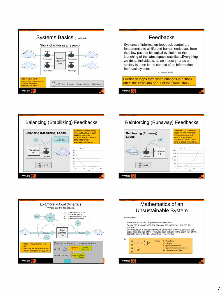
Example – Algal Dynamics- Where are the feedbacks?
Growth Mortality
• What do the dynamics look
like?
• What are the key interactions?
• What’s controlling the system?
Amax
Sh
Amax = Max Algal population
Sh = “Effective” shade
k = per-capita growth rate
kd = per-capita mortality
kd
k
𝑑𝐴
𝑑𝑡= 𝐺𝑟𝑜𝑤𝑡ℎ − 𝑀𝑜𝑟𝑡𝑎𝑙𝑖𝑡𝑦 overall dynamics
𝑆ℎ = (1 −𝐴
𝐴𝑚𝑎𝑥) shading factor
𝐺𝑟𝑜𝑤𝑡ℎ = 𝑘 𝐴 𝑆ℎ = 𝑘𝐴(1 −𝐴
𝐴𝑚𝑎𝑥) ;
Exponential
Growth
Density-
Dependence
Algal
Biomass
(A)
Modeling for Non-Modelers
Mathematics of an
Unsustainable SystemAssumptions:
• There are two pools: Population and Resource
• Resources are consumed at a constant per-capita rate, and are non-renewable
• The Population is influenced by birth and death: birth is a constant per-capita rate; the size of the Resource base influences the death rate of the population according to: Death Rate = 1-( R(t)/R0 )
So:
cPdt
dR
PR
Rb
dt
dP
0
1Where P = Population
R = Resource
b = per capita birth rate
c = per capita consumption rate
R0 = initial resource base
8
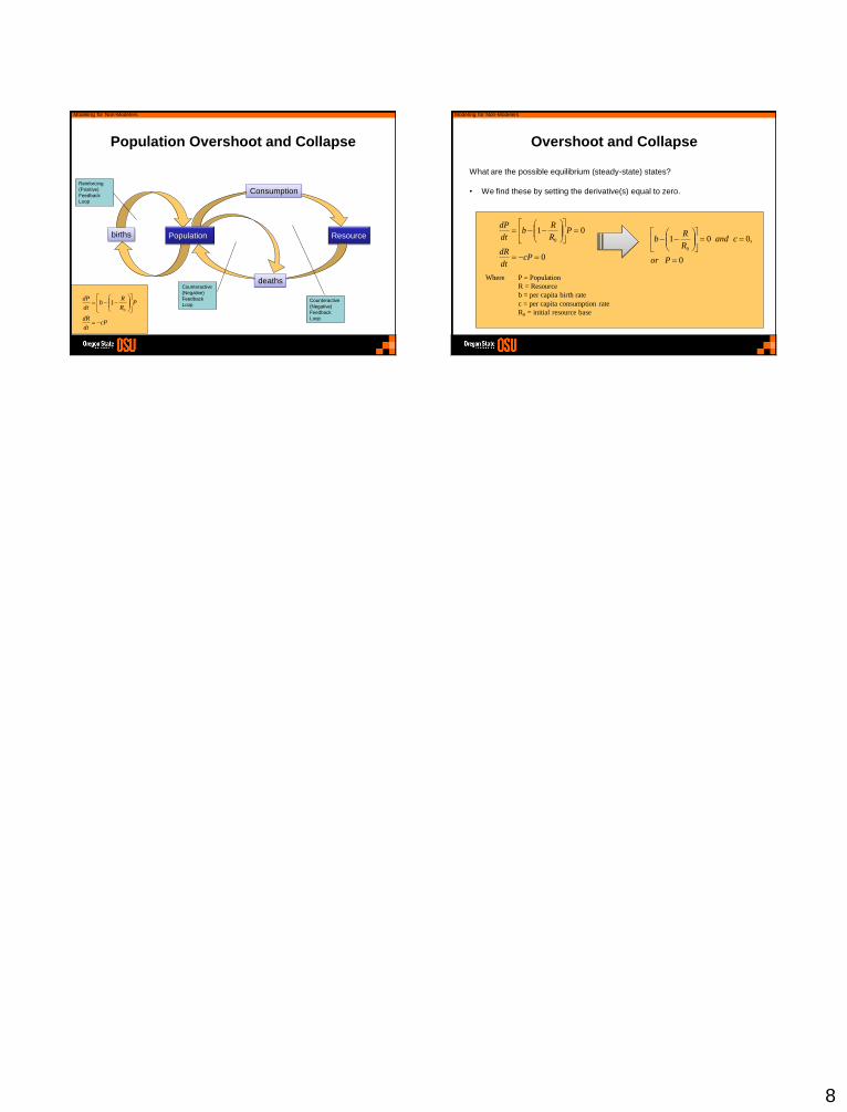
Modeling for Non-Modelers
cPdt
dR
PR
Rb
dt
dP
0
1
ResourcePopulation
deaths
births
ConsumptionReinforcing
(Positive)
Feedback
Loop
Counteractive
(Negative)
Feedback
LoopCounteractive
(Negative)
Feedback
Loop
Population Overshoot and Collapse
Modeling for Non-Modelers
Overshoot and Collapse
What are the possible equilibrium (steady-state) states?
• We find these by setting the derivative(s) equal to zero.
0
010
cPdt
dR
PR
Rb
dt
dP
Where P = Population
R = Resource
b = per capita birth rate
c = per capita consumption rate
R0 = initial resource base
0
,0010
Por
candR
Rb