model selection in linear regression

basic problem: how to choose between competing linear regression models model too small: "underfit" the data; poor predictions;

high bias; low variance model too big: "overfit" the data; poor predictions;

low bias; high variance model just right: balance bias and variance to get

good predictions

Bias-Variance Tradeoff

High Bias - Low Variance Low Bias - High Variance

“overfitting” - modeling the random component

Too Many Predictors?

When there are lots of X’s, get models with high variance and prediction suffers. Three “solutions:”

1.  Pick the “best” model

2.  Shrinkage/Ridge Regression

3.  Derived Inputs

Cross-validation Score: AIC, BIC All-subsets + leaps-and-bounds, Stepwise methods,

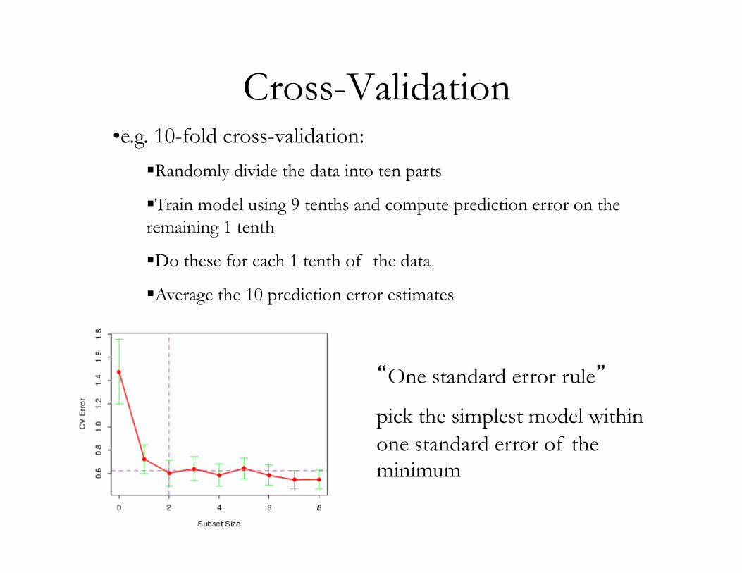
Cross-Validation

• e.g. 10-fold cross-validation:

§ Randomly divide the data into ten parts

§ Train model using 9 tenths and compute prediction error on the remaining 1 tenth

§ Do these for each 1 tenth of the data

§ Average the 10 prediction error estimates

“One standard error rule”

pick the simplest model within one standard error of the minimum

Library(DAAG)houseprices.lm <- lm(sale.price ~ area, data=houseprices)CVlm(houseprices,houseprices.lm,m=3)

fold 1 Observations in test set: 3 12 13 14 15 X11 X20 X21 X22 X23x=area 802.0 696 771.0 1006.0 1191Predicted 204.0 188 199.3 234.7 262sale.price 215.0 255 260.0 293.0 375Residual 11.0 67 60.7 58.3 113Sum of squares = 24000 Mean square = 4900 n = 5 fold 2 Observations in test set: 2 5 6 9 10 X10 X13 X14 X17 X18x=area 905 716 963.0 1018.00 887.00Predicted 255 224 264.4 273.38 252.06sale.price 215 113 185.0 276.00 260.00Residual -40 -112 -79.4 2.62 7.94Sum of squares = 20000 Mean square = 4100 n = 5

fold 3 Observations in test set: 1 4 7 8 11 X9 X12 X15 X16 X19x=area 694.0 1366 821.00 714.0 790.00Predicted 183.2 388 221.94 189.3 212.49sale.price 192.0 274 212.00 220.0 221.50Residual 8.8 -114 -9.94 30.7 9.01Sum of squares = 14000 Mean square = 2800 n = 5 Overall ms 3934

> summary(houseprices.lm)$sigma^2[1] 2321

> CVlm(houseprices,houseprices.lm,m=15)Overall ms 3247

Quicker solutions

• AIC and BIC try to mimic what cross-validation does

• AIC(MyModel)

• Smaller is better

Quicker solutions

• If have 15 predictors there are 215 different models (even before considering interactions, transformations, etc.) • “Leaps and bounds” is an efficient algorithm to do all-subsets

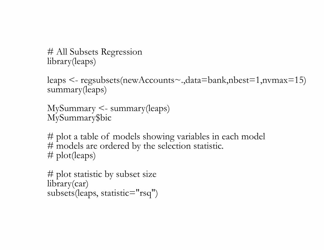
# All Subsets Regression library(leaps)

leaps <- regsubsets(newAccounts~.,data=bank,nbest=1,nvmax=15) summary(leaps)

MySummary <- summary(leaps) MySummary$bic # plot a table of models showing variables in each model # models are ordered by the selection statistic. # plot(leaps)

# plot statistic by subset size library(car) subsets(leaps, statistic="rsq")

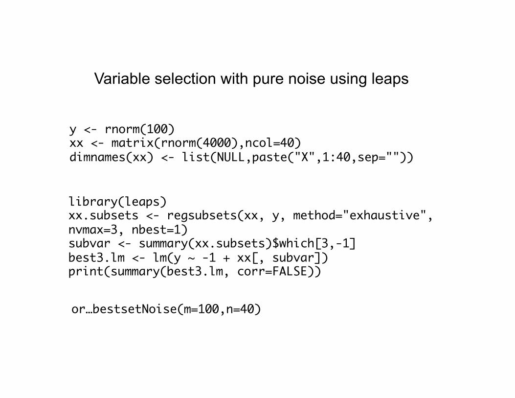
Variable selection with pure noise using leaps

y <- rnorm(100)xx <- matrix(rnorm(4000),ncol=40)dimnames(xx) <- list(NULL,paste("X",1:40,sep=""))

library(leaps)xx.subsets <- regsubsets(xx, y, method="exhaustive", nvmax=3, nbest=1)subvar <- summary(xx.subsets)$which[3,-1]best3.lm <- lm(y ~ -1 + xx[, subvar])print(summary(best3.lm, corr=FALSE))

or…bestsetNoise(m=100,n=40)

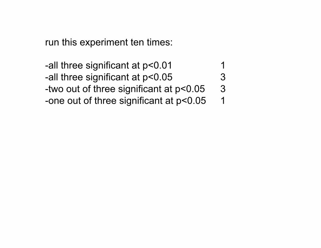
run this experiment ten times: - all three significant at p<0.01 1 - all three significant at p<0.05 3 - two out of three significant at p<0.05 3 - one out of three significant at p<0.05 1

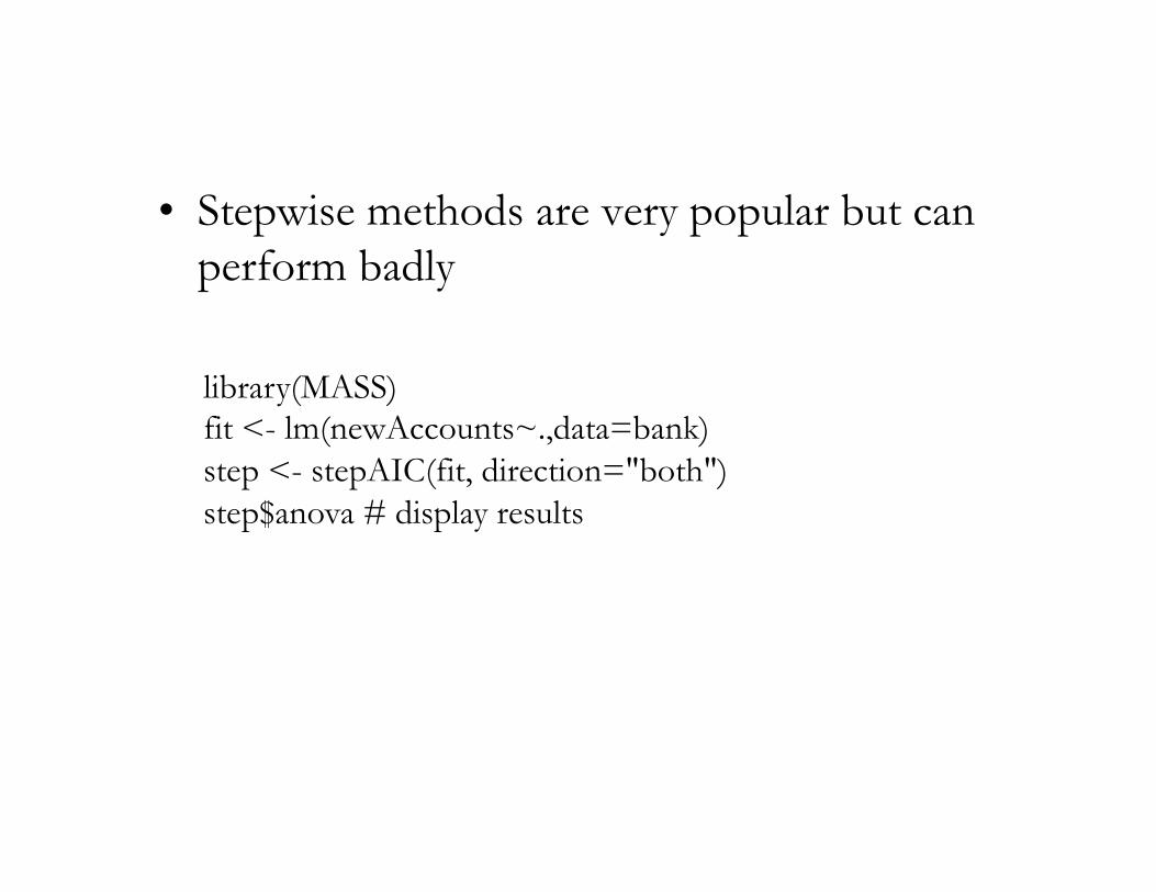
•  Stepwise methods are very popular but can perform badly

library(MASS) fit <- lm(newAccounts~.,data=bank) step <- stepAIC(fit, direction="both") step$anova # display results

Transformations

log, exp, sqrt, sqr, cube root, cube, etc. box-cox:

y(!) =(y ! "1) !, ! # 0log y, ! = 0

$ % &

bc <- function(x,l) {(x^l-1)/l}l<-seq(1,4,0.5)x<-seq(-3,3,0.1)par(new=FALSE)for (i in l) {

plot(x,bc(x,i),type="l",ylim=c(-20,20),col=2*i); par(new=TRUE)}legend("top",paste(l),col=2*l,lty=rep(1,length(l)))

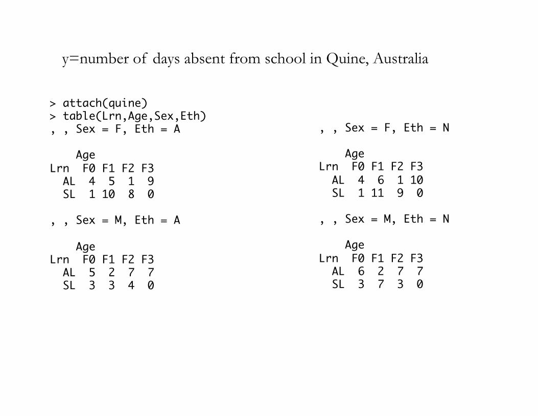
> attach(quine)> table(Lrn,Age,Sex,Eth), , Sex = F, Eth = A AgeLrn F0 F1 F2 F3 AL 4 5 1 9 SL 1 10 8 0, , Sex = M, Eth = A AgeLrn F0 F1 F2 F3 AL 5 2 7 7 SL 3 3 4 0

, , Sex = F, Eth = N AgeLrn F0 F1 F2 F3 AL 4 6 1 10 SL 1 11 9 0, , Sex = M, Eth = N AgeLrn F0 F1 F2 F3 AL 6 2 7 7 SL 3 7 3 0

y=number of days absent from school in Quine, Australia

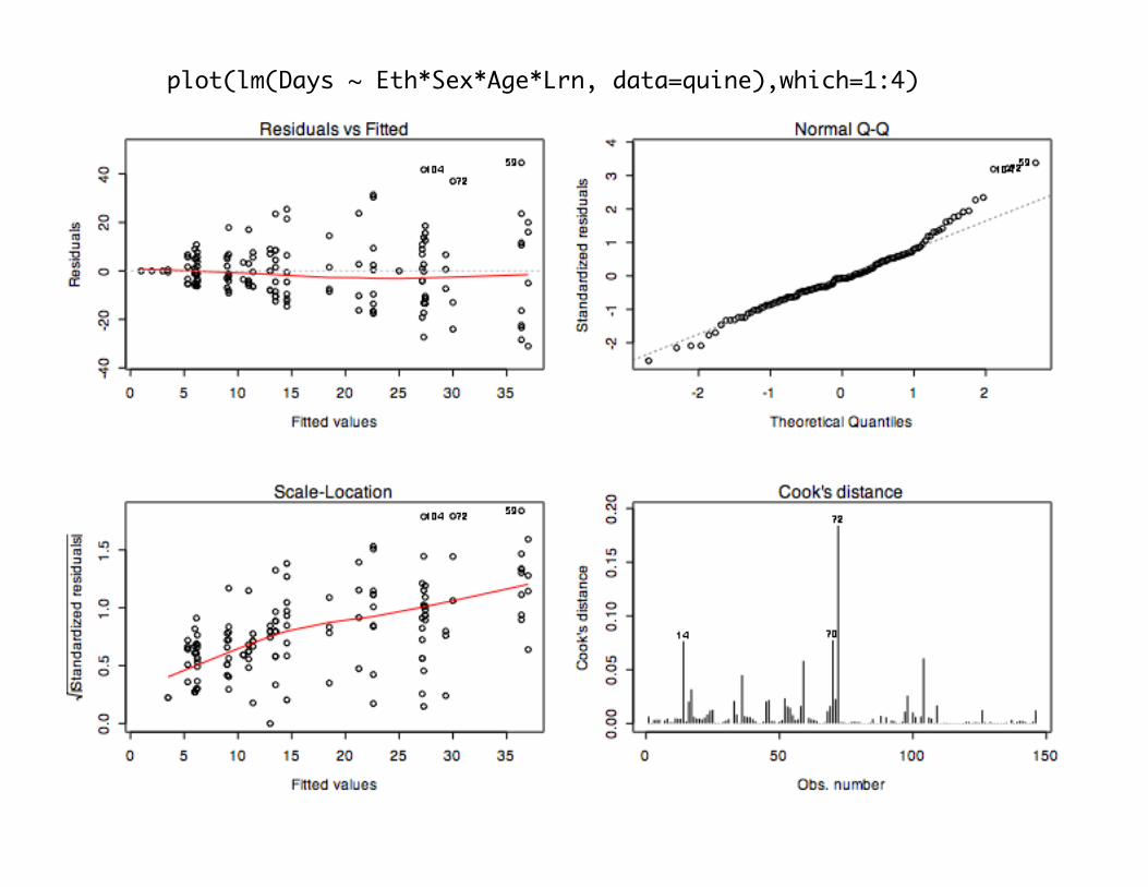
plot(lm(Days ~ Eth*Sex*Age*Lrn, data=quine),which=1:4)

> boxcox(Days+1 ~ Eth*Sex*Age*Lrn, data = quine, lambda = seq(-0.05, 0.45, len = 20))

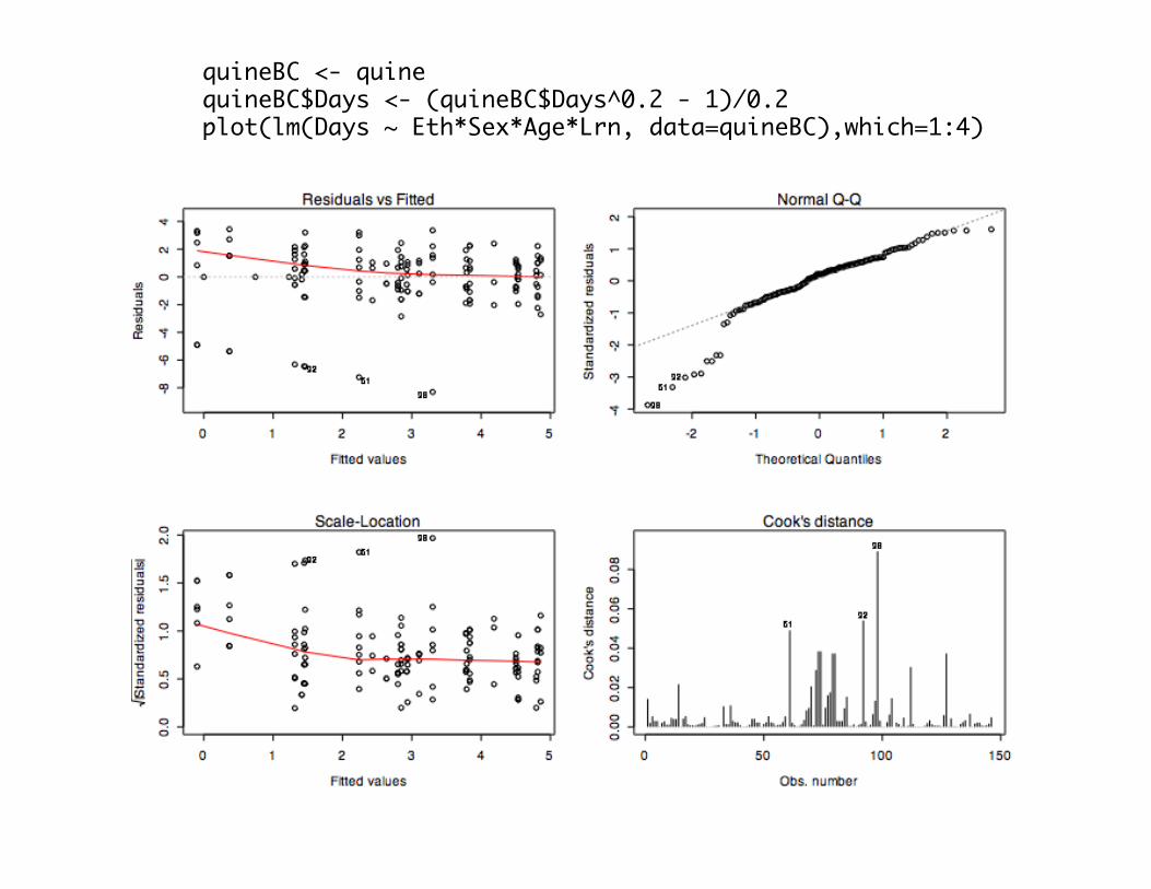
quineBC <- quinequineBC$Days <- (quineBC$Days^0.2 - 1)/0.2plot(lm(Days ~ Eth*Sex*Age*Lrn, data=quineBC),which=1:4)

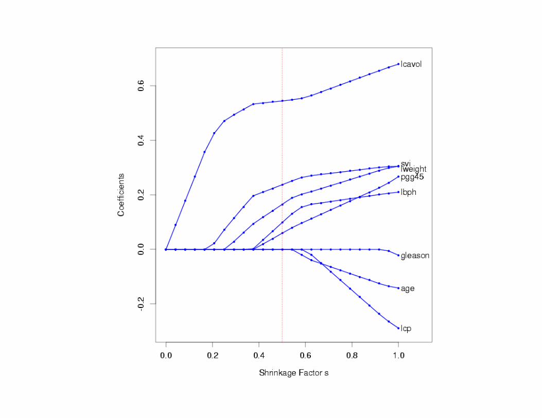
Shrinkage Methods

• Subset selection is a discrete process – individual variables are either in or out

• This method can have high variance – a different dataset from the same source can result in a totally different model

• Shrinkage methods allow a variable to be partly included in the model. That is, the variable is included but with a shrunken co-efficient.

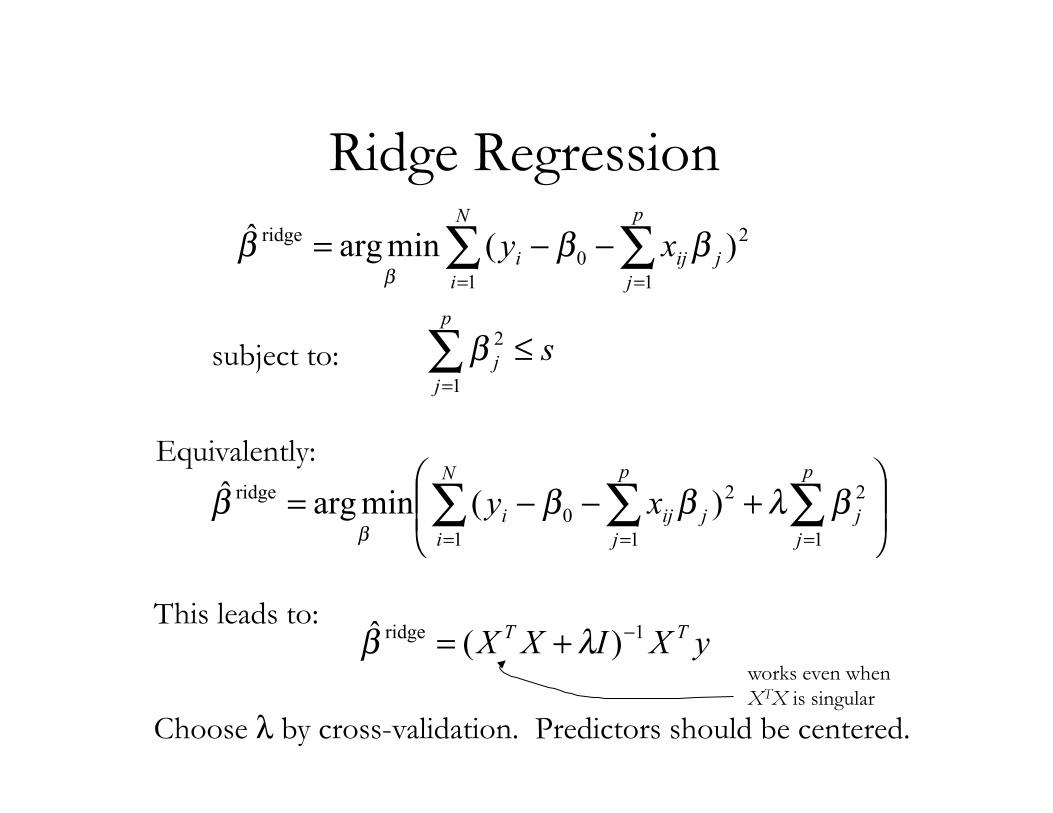
Ridge Regression

subject to:

2

1 10

ridge )(minargˆ ! != =

""=N

i

p

jjiji xy ###

#

!=

"p

jj s

1

2#

Equivalently:

!!"

#$$%

&+''= (( (

== =

p

jj

N

i

p

jjiji xy

1

22

1 10

ridge )(minargˆ )*))))

This leads to:

Choose λ by cross-validation. Predictors should be centered.

yXIXX TT 1ridge )(ˆ !+= "#works even when XTX is singular

effective number of X’s

The Lasso

subject to:

2

1 10

ridge )(minargˆ ! != =

""=N

i

p

jjiji xy ###

#

!=

"p

jj s

1#

Quadratic programming algorithm needed to solve for the parameter estimates. Choose s via cross-validation.

!!"

#$$%

&+''= (( (

== =

qp

jj

N

i

p

jjiji xy

1

2

1 10 )(minarg~ )*)))

)

q=0: var. sel. q=1: lasso q=2: ridge Learn q?

library(glmnet) bank <- read.table("/Users/dbm/Documents/W2025/BankSortedMissing.TXT",header=TRUE) names(bank) bank <- as.matrix(bank) x <- bank[1:200,-1] y <- bank[1:200,1] fit1 <- glmnet(x,y) xTest <- bank[201:233,-1] predict(fit1,newx=xTest,s=c(0.01,0.005)) predict(fit1,type="coef") plot(fit1,xvar="lambda") MyCV <- cv.glmnet(x,y)