model reduction and neural networks for parametric pdes

Journal of Computational MathematicsVol. 00, Pages 000–000 (XXXX)

Model Reduction And Neural Networks For Parametric PDEs

Kaushik Bhattacharya 1

Bamdad Hosseini 2

Nikola B. Kovachki 3

Andrew M. Stuart 4

1 Mechanical and Civil Engineering, California Institute of Technology, Pasadena, CA, USAEmail address: [email protected] Computing and Mathematical Sciences, California Institute of Technology, Pasadena, CA,USAEmail address: [email protected] Computing and Mathematical Sciences, California Institute of Technology, Pasadena, CA,USAEmail address: [email protected] Computing and Mathematical Sciences, California Institute of Technology, Pasadena, CA,USAEmail address: [email protected].

Abstract. We develop a general framework for data-driven approximation of input-output maps be-tween infinite-dimensional spaces. The proposed approach is motivated by the recent successes of neuralnetworks and deep learning, in combination with ideas from model reduction. This combination resultsin a neural network approximation which, in principle, is defined on infinite-dimensional spaces and,in practice, is robust to the dimension of finite-dimensional approximations of these spaces requiredfor computation. For a class of input-output maps, and suitably chosen probability measures on theinputs, we prove convergence of the proposed approximation methodology. We also include numericalexperiments which demonstrate the effectiveness of the method, showing convergence and robustnessof the approximation scheme with respect to the size of the discretization, and compare it with exist-ing algorithms from the literature; our examples include the mapping from coefficient to solution ina divergence form elliptic partial differential equation (PDE) problem, and the solution operator forviscous Burgers’ equation.

Keywords. approximation theory, deep learning, model reduction, neural networks, partial differentialequations.

2020 Mathematics Subject Classification. 65N75; 62M45; 68T05; 60H30; 60H15 .

1. Introduction

At the core of many computational tasks arising in science and engineering is the problem of repeatedlyevaluating the output of an expensive forward model for many statistically similar inputs. Such settingsinclude the numerical solution of parametric partial differential equations (PDEs), time-stepping forevolutionary PDEs and, more generally, the evaluation of input-output maps defined by black-boxcomputer models. The key idea in this paper is the development of a new data-driven emulator whichis defined to act between the infinite-dimensional input and output spaces of maps such as thosedefined by PDEs. By defining approximation architectures on infinite-dimensional spaces, we providethe basis for a methodology which is robust to the resolution of the finite-dimensionalizations used tocreate implementable algorithms.

This work is motivated by the recent empirical success of neural networks in machine learningapplications such as image classification, aiming to explore whether this success has any implicationsfor algorithm development in different applications arising in science and engineering. We further wishto compare the resulting new methods with traditional algorithms from the field of numerical analysis

1

arX

iv:2

005.

0318

0v2

[m

ath.

NA

] 1

7 Ju

n 20

21

mailto:[email protected]




K. Bhattacharya, B. Hosseini, N. Kovachki, & A. Stuart

for the approximation of infinite-dimensional maps, such as the maps defined by parametric PDEsor the solution operator for time-dependent PDEs. We propose a method for approximation of suchsolution maps purely in a data-driven fashion by lifting the concept of neural networks to producemaps acting between infinite-dimensional spaces. Our method exploits approximate finite-dimensionalstructure in maps between Banach spaces of functions through three separate steps: (i) reducing thedimension of the input; (ii) reducing the dimension of the output, and (iii) finding a map betweenthe two resulting finite-dimensional latent spaces. Our approach takes advantage of the approximationpower of neural networks while allowing for the use of well-understood, classical dimension reduction(and reconstruction) techniques. Our goal is to reduce the complexity of the input-to-output map byreplacing it with a data-driven emulator. In achieving this goal we design an emulator which enjoysmesh-independent approximation properties, a fact which we establish through a combination of theoryand numerical experiments; to the best of our knowledge, these are the first such results in the areaof neural networks for PDE problems.

To be concrete, and to guide the literature review which follows, consider the following prototypicalparametric PDE

(Pxy)(s) = 0, ∀s ∈ D,where D ⊂ Rd is a bounded open set, Px is a differential operator depending on a parameter x ∈ Xand y ∈ Y is the solution to the PDE (given appropriate boundary conditions). The Banach spacesX and Y are assumed to be spaces of real-valued functions on D. Here, and in the rest of this paper,we consistently use s to denote the independent variable in spatially dependent PDEs, and reserve xand y for the input and output of the PDE model of interest. We adopt this idiosyncratic notation(from the PDE perspective) to keep our exposition in line with standard machine learning notationfor input and output variables.

Example 1.1. Consider second order elliptic PDEs of the form

−∇ · (a(s)∇u(s)) = f(s), s ∈ Du(s) = 0, s ∈ ∂D

(1.1)

which are prototypical of many scientific applications. As a concrete example of a mapping defined bythis equation, we restrict ourselves to the setting where the forcing term f is fixed, and consider thediffusion coefficient a as the input parameter x and the PDE solution u as output y. In this setting,we have X = L∞(D;R+), Y = H1

0 (D;R), and Px = −∇s · (a∇s·) − f , equipped with homogeneousDirichlet boundary conditions. This is the Darcy flow problem which we consider numerically in Section4.3.

1.1. Literature Review

The recent success of neural networks on a variety of high-dimensional machine learning problems[49] has led to a rapidly growing body of research pertaining to applications in scientific problems[1, 7, 13, 25, 30, 39, 68, 83, 76]. In particular, there is a substantial number of articles which investigatethe use of neural networks as surrogate models, and more specifically for obtaining the solution of(possibly parametric) PDEs.

We summarize the two most prevalent existing neural network based strategies in the approximationof PDEs in general, and parametric PDEs specifically. The first approach can be thought of as image-to-image regression. The goal is to approximate the parametric solution operator mapping elementsof X to Y. This is achieved by discretizing both spaces to obtain finite-dimensional input and outputspaces of dimension K. We assume to have access to data in the form of observations of input x andoutput y discretized on K-points within the domain D. The methodology then proceeds by defining aneural network F : RK → RK and regresses the input-to-output map by minimizing a misfit functional

2

MODEL REDUCTION AND NEURAL NETWORKS FOR PARAMETRIC PDES

defined using the point values of x and y on the discretization grid. The articles [1, 7, 39, 83, 29] applythis methodology for various forward and inverse problems in physics and engineering, utilizing avariety of neural network architectures in the regression step; the related paper [42] applies a similarapproach, but the output space is R. This innovative set of papers demonstrate some success. However,from the perspective of the goals of our work, their approaches are not robust to mesh-refinement: theneural network is defined as a mapping between two Euclidean spaces of values on mesh points. Therates of approximation depend on the underlying discretization and an overhaul of the architecturewould be required to produce results consistent across different discretizations. The papers [54, 55]make a conceptual step in the direction of interest to us in this paper, as they introduce an architecturebased on a neural network approximation theorem for operators from [12]; but as implemented themethod still results in parameters which depend on the mesh used. Applications of this methodologymay be found in [11, 58, 52].

The second approach does not directly seek to find the parametric map from X to Y but ratheris thought of, for fixed x ∈ X , as being a parametrization of the solution y ∈ Y by means of adeep neural network [24, 25, 40, 47, 68, 75]. This methodology parallels collocation methods for thenumerical solution of PDEs by searching over approximation spaces defined by neural networks. Thesolution of the PDE is written as a neural network approximation in which the spatial (or, in thetime-dependent case, spatio-temporal) variables in D are inputs and the solution is the output. Thisparametric function is then substituted into the PDE and the residual is made small by optimization.The resulting neural network may be thought of as a novel structure which composes the action of theoperator Px, for fixed x, with a neural network taking inputs in D [68]. While this method leads to anapproximate solution map defined on the input domain D (and not on a K−point discretization of thedomain), the parametric dependence of the approximate solution map is fixed. Indeed for a new inputparameter x, one needs to re-train the neural network by solving the associated optimization problemin order to produce a new map y : D → R; this may be prohibitively expensive when parametricdependence of the solution is the target of analysis. Furthermore the approach cannot be made fullydata-driven as it needs knowledge of the underlying PDE, and furthermore the operations required toapply the differential operator may interact poorly with the neural network approximator during theback-propagation (adjoint calculation) phase of the optimization.

The work [70] examines the forward propagation of neural networks as the flow of a time-dependentPDE, combining the continuous time formulation of ResNet [34, 80] with the idea of neural networksacting on spaces of functions: by considering the initial condition as a function, this flow map may bethought of as a neural network acting between infinite-dimensional spaces. The idea of learning PDEsfrom data using neural networks, again generating a flow map between infinite dimensional spaces,was studied in the 1990s in the papers [44, 32] with the former using a PCA methodology, and thelatter using the method of lines. More recently the works [37, 79] also employ a PCA methodologyfor the output space but only consider very low dimensional input spaces. Furthermore the works[50, 28, 31, 28] proposed a model reduction approach for dynamical systems by use of dimensionreducing neural networks (autoencoders). However only a fixed discretization of space is considered,yielding a method which does not produce a map between two infinite-dimensional spaces.

The development of numerical methods for parametric problems is not, of course, restricted to theuse of neural networks. Earlier works in the engineering literature started in the 1970s focused oncomputational methods which represent PDE solutions in terms of known basis functions that containinformation about the solution structure [2, 61]. This work led to the development of the reducedbasis method (RBM) which is widely adopted in engineering; see [3, 36, 67] and the references therein.The methodology was also used for stochastic problems, in which the input space X is endowed witha probabilistic structure, in [10]. The study of RBMs led to broader interest in the approximationtheory community focusing on rates of convergence for the RBM approximation of maps between

3


Banach spaces, and in particular maps defined through parametric dependence of PDEs; see [23] foran overview of this work.

Ideas from model reduction have been combined with data-driven learning in the sequence of papers[65, 59, 6, 64, 66]. The setting is the learning of data-driven approximations to time-dependent PDEs.Model reduction is used to find a low-dimensional approximation space and then a system of ordinarydifferential equations (ODEs) is learned in this low-dimensional latent space. These ODEs are assumedto have vector fields from a known class with unknown linear coefficients; learning is thus reduced to aleast squares problem. The known vector fields mimic properties of the original PDE (for example arerestricted to linear and quadratic terms for the equations of geophysical fluid dynamics); additionallytransformations may be used to render the original PDE in a desirable form form (such as having onlyquadratic nonlinearities.)

The development of theoretical analyses to understand the use of neural networks to approximatePDEs is currently in its infancy, but interesting results are starting to emerge [35, 45, 71, 46]. Arecurrent theme in the analysis of neural networks, and in these papers in particular, is that thework typically asserts the existence of a choice of neural network parameters which achieve a certainapproximation property; because of the non-convex optimization techniques used to determine thenetwork parameters, the issue of finding these parameters in practice is rarely addressed. Recentworks take a different perspective on data-driven approximation of PDEs, motivated by small-datascenarios; see the paper [16] which relates, in part, to earlier work focused on the small-data setting[8, 56]. These approaches are more akin to data assimilation [69, 48] where the data is incorporatedinto a model.

1.2. Our Contribution

The primary contributions of this paper are as follows:

(1) we propose a novel data-driven methodology capable of learning mappings between Hilbertspaces;

(2) the proposed method combines model reduction with neural networks to obtain algorithmswith controllable approximation errors as maps between Hilbert spaces;

(3) as a result of this approximation property of maps between Hilbert spaces, the learned mapsexhibit desirable mesh-independence properties;

(4) we prove that our architecture is sufficiently rich to contain approximations of arbitrary accu-racy, as a mapping between function spaces;

(5) we present numerical experiments that demonstrate the efficacy of the proposed methodology,demonstrate desirable mesh-indepence properties, elucidate its properties beyond the confinesof the theory, and compare with other methods for parametric PDEs.

Section 2 outlines the approximation methodology, which is based on use of principal componentanalysis (PCA) in a Hilbert space to finite-dimensionalize the input and output spaces, and a neuralnetwork between the resulting finite-dimensional spaces. Section 3 contains statement and proof of ourmain approximation result, which invokes a global Lipschitz assumption on the map to be approxi-mated. In Section 4 we present our numerical experiments, some of which relax the global Lipschitzassumption, and others which involve comparisons with other approaches from the literature. Section5 contains concluding remarks, including directions for further study. We also include auxiliary re-sults in the appendix that complement and extend the main theoretical developments of the article.Appendix A extends the analysis of Section 3 from globally Lipschitz maps to locally Lipschitz maps

4


X RdX X

Y RdY Y

FX

Ψ

GX

ϕ Ψ

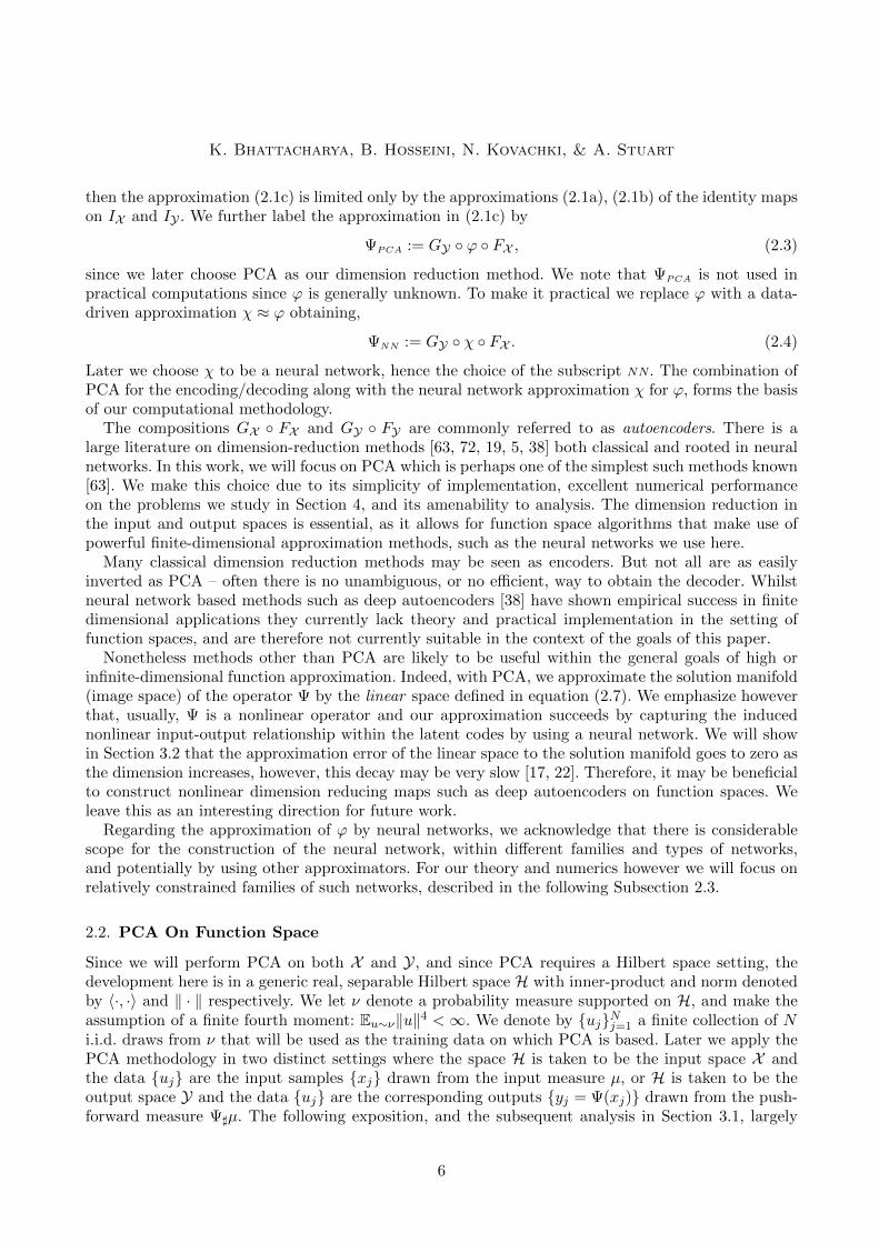
FY GY

Figure 1. A diagram summarizing various maps of interest in our proposed approachfor the approximation of input-output maps between infinite-dimensional spaces.

with controlled growth rates. Appendix B contains supporting lemmas that are used throughout thepaper while Appendix C proves an analyticity result pertaining to the solution map of the Poissonequation that is used in one of the numerical experiments in Section 4.

2. Proposed Method

Our method combines PCA-based dimension reduction on the input and output spaces X ,Y with aneural network that maps the dimension-reduced spaces. After a pre-amble in Subsection 2.1, givingan overview of our approach, we continue in Subsection 2.2 with a description of PCA in the Hilbertspace setting, including intuition about its approximation quality. Subsection 2.3 gives the backgroundon neural networks needed for this paper, and Subsection 2.4 compares our methodology to existingmethods.

2.1. Overview

Let X , Y be separable Hilbert spaces and Ψ : X → Y be some, possibly nonlinear, map. Our goalis to approximate Ψ from a finite collection of evaluations xj , yjNj=1 where yj = Ψ(xj). We assume

that the xj are i.i.d. with respect to (w.r.t.) a probability measure µ supported on X . Note that withthis notation the output samples yj are i.i.d. w.r.t. the push-forward measure Ψ]µ. The approximation

of Ψ from the data xj , yjNj=1 that we now develop should be understood as being designed to beaccurate with respect to norms defined by integration with respect to the measures µ and Ψ]µ on thespaces X and Y respectively.

Instead of attempting to directly approximate Ψ, we first try to exploit possible finite-dimensionalstructure within the measures µ and Ψ]µ. We accomplish this by approximating the identity mappingsIX : X → X and IY : Y → Y by a composition of two maps, known as the encoder and the decoder inthe machine learning literature [38, 33], which have finite-dimensional range and domain, respectively.We will then interpolate between the finite-dimensional outputs of the encoders, usually referred toas the latent codes. Our approach is summarized in Figure 1.

Here, FX and FY are the encoders for the spaces X ,Y respectively, whilst GX and GY are thedecoders, and ϕ is the map interpolating the latent codes. The intuition behind Figure 1, and, to someextent, the main focus of our analysis, concerns the quality of the the approximations

GX FX ≈ IX , (2.1a)

GY FY ≈ IY , (2.1b)

GY ϕ FX ≈ Ψ. (2.1c)

In order to achieve (2.1c) it is natural to choose ϕ as

ϕ := FY Ψ GX ; (2.2)

5


then the approximation (2.1c) is limited only by the approximations (2.1a), (2.1b) of the identity mapson IX and IY . We further label the approximation in (2.1c) by

ΨPCA := GY ϕ FX , (2.3)

since we later choose PCA as our dimension reduction method. We note that ΨPCA is not used inpractical computations since ϕ is generally unknown. To make it practical we replace ϕ with a data-driven approximation χ ≈ ϕ obtaining,

ΨNN := GY χ FX . (2.4)

Later we choose χ to be a neural network, hence the choice of the subscript NN. The combination ofPCA for the encoding/decoding along with the neural network approximation χ for ϕ, forms the basisof our computational methodology.

The compositions GX FX and GY FY are commonly referred to as autoencoders. There is alarge literature on dimension-reduction methods [63, 72, 19, 5, 38] both classical and rooted in neuralnetworks. In this work, we will focus on PCA which is perhaps one of the simplest such methods known[63]. We make this choice due to its simplicity of implementation, excellent numerical performanceon the problems we study in Section 4, and its amenability to analysis. The dimension reduction inthe input and output spaces is essential, as it allows for function space algorithms that make use ofpowerful finite-dimensional approximation methods, such as the neural networks we use here.

Many classical dimension reduction methods may be seen as encoders. But not all are as easilyinverted as PCA – often there is no unambiguous, or no efficient, way to obtain the decoder. Whilstneural network based methods such as deep autoencoders [38] have shown empirical success in finitedimensional applications they currently lack theory and practical implementation in the setting offunction spaces, and are therefore not currently suitable in the context of the goals of this paper.

Nonetheless methods other than PCA are likely to be useful within the general goals of high orinfinite-dimensional function approximation. Indeed, with PCA, we approximate the solution manifold(image space) of the operator Ψ by the linear space defined in equation (2.7). We emphasize howeverthat, usually, Ψ is a nonlinear operator and our approximation succeeds by capturing the inducednonlinear input-output relationship within the latent codes by using a neural network. We will showin Section 3.2 that the approximation error of the linear space to the solution manifold goes to zero asthe dimension increases, however, this decay may be very slow [17, 22]. Therefore, it may be beneficialto construct nonlinear dimension reducing maps such as deep autoencoders on function spaces. Weleave this as an interesting direction for future work.

Regarding the approximation of ϕ by neural networks, we acknowledge that there is considerablescope for the construction of the neural network, within different families and types of networks,and potentially by using other approximators. For our theory and numerics however we will focus onrelatively constrained families of such networks, described in the following Subsection 2.3.

2.2. PCA On Function Space

Since we will perform PCA on both X and Y, and since PCA requires a Hilbert space setting, thedevelopment here is in a generic real, separable Hilbert space H with inner-product and norm denotedby 〈·, ·〉 and ‖ · ‖ respectively. We let ν denote a probability measure supported on H, and make theassumption of a finite fourth moment: Eu∼ν‖u‖4 <∞. We denote by ujNj=1 a finite collection of Ni.i.d. draws from ν that will be used as the training data on which PCA is based. Later we apply thePCA methodology in two distinct settings where the space H is taken to be the input space X andthe data uj are the input samples xj drawn from the input measure µ, or H is taken to be theoutput space Y and the data uj are the corresponding outputs yj = Ψ(xj) drawn from the push-forward measure Ψ]µ. The following exposition, and the subsequent analysis in Section 3.1, largely

6


follows the works [9, 73, 74]. We will consider the standard version of non-centered PCA, althoughmore sophisticated versions such as kernel PCA have been widely used and analyzed [72] and couldbe of potential interest within the overall goals of this work. We choose to work in the non-kernelizedsetting as there is an unequivocal way of producing the decoder.

For any subspace V ⊆ H, denote by ΠV : H → V the orthogonal projection operator and definethe empirical projection error,

RN (V ) :=1

N

N∑j=1

‖uj −ΠV uj‖2. (2.5)

PCA consists of projecting the data onto a finite-dimensional subspace of H for which this error isminimal. To that end, consider the empirical, non-centered covariance operator

CN :=1

N

N∑j=1

uj ⊗ uj (2.6)

where ⊗ denotes the outer product. It may be shown that CN is a non-negative, self-adjoint, trace-class operator on H, of rank at most N [82]. Let φ1,N , . . . φN,N denote the eigenvectors of CN andλ1,N ≥ λ2,N ≥ · · · ≥ λN,N ≥ 0 its corresponding eigenvalues in decreasing order. Then for any d ≥ 1we define the PCA subspaces

Vd,N = spanφ1,N , φ2,N , . . . , φd,N ⊂ H. (2.7)

It is well known [60, Thm. 12.2.1] that Vd,N solves the minimization problem

minV ∈Vd

RN (V ),

where Vd denotes the set of all d-dimensional subspaces of H. Furthermore

RN (Vd,N ) =N∑

j=d+1

λj,N , (2.8)

hence the approximation is controlled by the rate of decay of the spectrum of CN .With this in mind, we define the PCA encoder FH : H → Rd as the mapping from H to the

coefficients of the orthogonal projection onto Vd,N namely,

FH(u) = (〈u, φ1,N 〉, . . . , 〈u, φd,N 〉)T ∈ Rd. (2.9)

Correspondingly, the PCA decoder GH : Rd → H constructs an element of H by taking as its inputthe coefficients constructed by FH and forming an expansion in the empirical basis by zero-paddingthe PCA basis coefficients, that is

GH(s) =

d∑j=1

sjφj,N ∀s ∈ Rd. (2.10)

In particular,

(GH FH)(u) =

d∑j=1

〈u, φj,N 〉φj,N , equivalently GH FH =

d∑j=1

φj,N ⊗ φj,N .

Hence GH FH = ΠVd,N , a d-dimensional approximation to the identity IH.We will now give a qualitative explanation of this approximation to be made quantitative in Sub-

section 3.1. It is natural to consider minimizing the infinite data analog of (2.5), namely the projectionerror

R(V ) := Eu∼ν‖u−ΠV u‖2, (2.11)

7


over Vd for d ≥ 1. Assuming ν has a finite second moment, there exists a unique, self-adjoint, non-negative, trace-class operator C : H → H termed the non-centered covariance such that 〈v, Cz〉 =Eu∼ν [〈v, u〉〈z, u〉], ∀v, z ∈ H (see [4]). From this, one readily finds the form of C by noting that

〈v,Eu∼ν [u⊗ u]z〉 = Eu∼ν [〈v, (u⊗ u)z〉] = Eu∼ν [〈v, u〉〈z, u〉], (2.12)

implying that C = Eu∼ν [u⊗ u]. Moreover, it follows that

tr C = Eu∼ν [tr u⊗ u] = Eu∼ν‖u‖2 <∞.Let φ1, φ2, . . . denote the eigenvectors of C and λ1 ≥ λ2 ≥ . . . the corresponding eigenvalues. In the

infinite data setting (N =∞) it is natural to think of C and its first d eigenpairs as known. We thendefine the optimal projection space

Vd = spanφ1, φ2, . . . , φd. (2.13)

It may be verified that Vd solves the minimization problem minV ∈Vd R(V ) and thatR(Vd) =∑∞

j=d+1 λj .With this infinite data perspective in mind observe that PCA makes the approximation Vd,N ≈ Vd

from a finite dataset. The approximation quality of Vd,N w.r.t. Vd is related to the approximationquality of φj by φj,N for j = 1, . . . , N and therefore to the approximation quality of C by CN .Another perspective is via the Karhunen-Loeve Theorem (KL) [53]. For simplicity, assume that νis mean zero, then u ∼ ν admits an expansion of the form u =

∑∞j=1

√λjξjφj where ξj∞j=1 is a

sequence of scalar-valued, mean zero, pairwise uncorrelated random variables. We can then truncatethis expansion and make the approximations

u ≈d∑j=1

√λjξjφj ≈

d∑j=1

√λj,Nξjφj,N ,

where the first approximation corresponds to using the optimal projection subspace Vd while thesecond approximation replaces Vd with Vd,N . Since it holds that ECN = C, we expect λj ≈ λj,N andφj ≈ φj,N . These discussions suggest that the quality of the PCA approximation is controlled, onaverage, by the rate of decay of the eigenvalues of C, and the approximation of the eigenstructure ofC by that of CN .

2.3. Neural Networks

A neural network is a nonlinear function χ : Rn → R defined by a sequence of compositions of affinemaps with point-wise nonlinearities. In particular,

χ(s) = Wtσ(. . . σ(W2σ(W1s+ b1) + b2)) + bt, s ∈ Rn, (2.14)

where W1, . . . ,Wt are weight matrices (that are not necessarily square) and b1, . . . , bt are vectors,referred to as biases. We refer to t ≥ 1 as the depth of the neural network. The function σ : Rd → Rdis a monotone, nonlinear activation function that is defined from a monoton function σ : R → Rapplied entrywise to any vector in Rd with d ≥ 1. Note that in (2.14) the input dimension of σ mayvary between layers but regardless of the input dimension the function σ applies the same operationsto all entries of the input vector. We primarily consider the Rectified Linear Unit (ReLU) activationfunctions, i.e.,

σ(s) := (max0, s1,max0, s2, . . . ,max0, sd)T ∈ Rd ∀s ∈ Rd. (2.15)

The weights and biases constitute the parameters of the network. In this paper we learn theseparameters in the following standard way [49]: given a set of data xj , yjNj=1 we choose the parametersof χ to solve an appropriate regression problem by minimizing a data-dependent cost functional, usingstochastic gradient methods. Neural networks have been demonstrated to constitute an efficient classof regressors and interpolators for high-dimensional problems empirically, but a complete theory of

8


their efficacy is elusive. For an overview of various neural network architectures and their applications,see [33]. For theories concerning their approximation capabilities see [57, 81, 71, 21, 45].

For the approximation results given in Section 3, we will work with a specific class of neural networks,following [81]; we note that other approximation schemes could be used, however, and that we havechosen a proof setting that aligns with, but is not identical to, what we implement in the computationsdescribed in Section 4. We will fix σ ∈ C(R;R) to be the ReLU function (2.15) and consider the setof neural networks mapping Rn to R

M(n; t, r) :=

χ(s) = Wtσ(. . . σ(W2σ(W1s+ b1) + b2)) + bt ∈ R,

for all s ∈ Rn and such thatt∑

k=1

|Wk|0 + |bk|0 ≤ r.

Here | · |0 gives the number of non-zero entries in a matrix so that r ≥ 0 denotes the number of activeweights and biases in the network while t ≥ 1 is the total number of layers. Moreover, we define theclass of stacked neural networks mapping Rn to Rm:

M(n,m; t, r) :=

χ(s) = (χ(1)(s), . . . , χ(m)(s))T ∈ Rm,

where χ(j) ∈M(n; t(j), r(j)), with t(j) ≤ t, r(j) ≤ r.

From this, we build the set of zero-extended neural networks

M(n,m; t, r,M) :=

χ =

χ(s), s ∈ [−M,M ]n

0, s 6∈ [−M,M ]n

, for some χ ∈M(n,m, t, r)

,

where the new parameter M > 0 is the side length of the hypercube in Rn within which χ can be non-zero. This construction is essential to our approximation as it allows us to handle non-compactness ofthe latent spaces after PCA dimension reduction.

2.4. Comparison to Existing Methods

In the general setting of arbitrary encoders, the formula (2.1c) for the approximation of Ψ yields acomplicated map, the representation of which depends on the dimension reduction methods beingemployed. However, in the setting where PCA is used, a clear representation emerges which we nowelucidate in order to highlight similarities and differences between our methodology and existingmethods appearing in the literature.

Let FX : X → RdX be the PCA encoder w.r.t. the data xjNj=1 given by (2.9) and, in particular, let

φX1,N , . . . , φXdX ,N

be the eigenvectors of the resulting empirical covariance. Similarly let φY1,N , . . . , φYdY ,N

be the eigenvectors of the empirical covariance w.r.t. the data yNj=1. For the function ϕ defined

in (2.2), or similarly for approximations χ thereof found through the use of neural networks, wedenote the components by ϕ(s) = (ϕ1(s), . . . , ϕdY (s)) for any s ∈ RdX . Then (2.1c) becomes Ψ(x) ≈∑dY

j=1 αj(x)φYj,N with coefficients

αj(x) = ϕj(FX (x)

)= ϕj

(〈x, φX1,N 〉X , . . . , 〈x, φXdX ,N 〉X

), ∀x ∈ X .

The solution data yNj=1 fixes a basis for the output space, and the dependence of Ψ(x) on x iscaptured solely via the scalar-valued coefficients αj . This parallels the formulation of the classicalreduced basis method [23] where the approximation is written as

Ψ(x) ≈m∑j=1

αj(x)φj . (2.16)

9


Many versions of the method exist, but two particularly popular ones are: (i) when m = N and

φj = yj ; and (ii) when, as is done here, m = dY and φj = φYj,N . The latter choice is also referred to asthe reduced basis with a proper orthogonal decomposition.

The crucial difference between our method and the RBM is in the formation of the coefficients αj . InRBM these functions are obtained in an intrusive manner by approximating the PDE within the finite-dimensional reduced basis and as a consequence the method cannot be used in a setting where a PDErelating inputs and outputs is not known, or may not exist. In contrast, our proposed methodologyapproximates ϕ by regressing or interpolating the latent representations FX (xj), FY(yj)Nj=1. Thusour proposed method makes use of the entire available dataset and does not require explicit knowledgeof the underlying PDE mapping, making it a non-intrusive method applicable to black-box models.

The form (2.16) of the approximate solution operator can also be related to the Taylor approx-imations developed in [14, 18] where a particular form of the input x is considered, namely x =x +

∑j≥1 aj xj where x ∈ X is fixed, ajj≥1 ∈ `∞(N;R) are uniformly bounded, and xjj≥1 ∈ X

have some appropriate norm decay. Then, assuming that the solution operator Ψ : X → Y is analytic[15], it is possible to make use of the Taylor expansion

Ψ(x) =∑h∈F

αh(x)ψh,

where F = h ∈ N∞ : |h|0 <∞ is the set of multi-indices and

αh(x) =∏j≥1

ahjj ∈ R, ψh =

1

h!∂hΨ(0) ∈ Y;

here the differentiation ∂h is with respect to the sequence of coefficients ajj≥1. Then Ψ is approx-imated by truncating the Taylor expansion to a finite subset of F . For example this may be donerecursively, by starting with h = 0 and building up the index set in a greedy manner. The method isnot data-driven, and requires knowledge of the PDE to define equations to be solved for the ψh.

3. Approximation Theory

In this section, we prove our main approximation result: given any ε > 0, we can find an ε−approximationΨNN of Ψ. We achieve this by making the appropriate choice of PCA truncation parameters, bychoosing sufficient amounts of data, and by choosing a sufficiently rich neural network architecture toapproximate ϕ by χ.

In what follows we define FX to be a PCA encoder given by (2.9), using the input data xjNj=1

drawn i.i.d. from µ, and GY to be a PCA decoder given by (2.10), using the data yj = Ψ(xj)Nj=1.We also define

eNN(x) = ‖(GY χ FX )(x)−Ψ(x)‖Y= ‖ΨNN(x)−Ψ(x)‖Y .

We prove the following theorem:

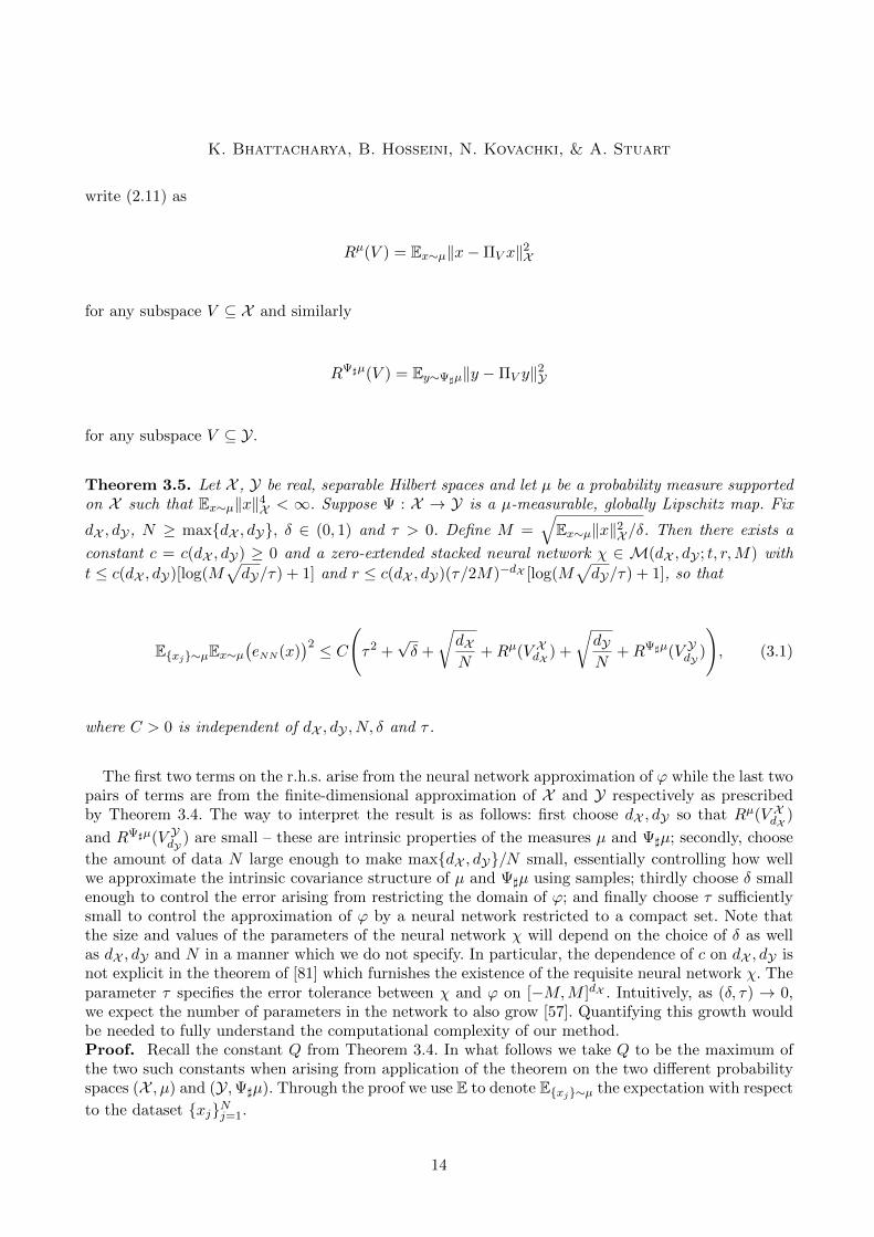
Theorem 3.1. Let X , Y be real, separable Hilbert spaces and let µ be a probability measure supportedon X such that Ex∼µ‖x‖4X < ∞. Suppose Ψ : X → Y is a µ-measurable, globally Lipschitz map.For any ε > 0, there are dimensions dX = dX (ε) ∈ N, dY = dY(ε) ∈ N, a requisite amount of dataN = N(dX , dY) ∈ N, parameters t, r,M depending on dX , dY and ε, and a zero-extended stacked neuralnetwork χ ∈M(dX , dY ; t, r,M) such that

Exj∼µEx∼µ(eNN(x)2

)< ε.

10


Remark 3.2. This theorem is a consequence of Theorem 3.5 which we state and prove below. Forclarity and ease of exposition we state and prove Theorem 3.5 in a setting where Ψ is globally Lipschitz.With a more stringent moment condition on µ, the result can also be proven when Ψ is locally Lipschitz;we state and prove this result in Theorem A.1.

Remark 3.3. The neural network χ ∈ M(dX , dY ; t, r,M) has maximum number of layers t ≤c[log(M2dY/ε) + 1], with the number of active weights and biases in each component of the net-

work r ≤ c(ε/4M2)−dX /2[log(M2dY/ε) + 1], with an appropriate constant c = c(dX , dY) ≥ 0 andsupport side-length M = M(dX , dY) > 0. These bounds on t and r follow from Theorem 3.5 with

τ = ε12 . Note, however, that in order to achieve error ε, the dimensions dX , dY must be chosen to grow

as ε→ 0; thus the preceding statements do not explicitly quantify the needed number of parameters,and depth, for error ε; to do so would require quantifying the dependence of c,M on dX , dY (a propertyof neural networks) and the dependence of dX , dY on ε (a property of the measure µ and spaces X ,Y –see Theorem 3.4). The theory in [81], which we employ for the existence result for the neural networkproduces the constant c which depends on the dimensions dX and dY in an unspecified way.

The double expectation reflects averaging over all possible new inputs x drawn from µ (inner expec-tation) and over all possible realizations of the i.i.d. dataset xj , yj = Ψ(xj)Nj=1 (outer expectation).The theorem as stated above is a consequence of Theorem 3.5 in which the error is broken into multiplecomponents that are then bounded separately. Note that the theorem does not address the questionof whether the optimization technique used to fit the neural network actually finds the choice whichrealizes the theorem; this gap between theory and practice is difficult to overcome, because of thenon-convex nature of the training problem, and is a standard feature of theorems in this area [45, 71].

The idea of the proof is to quantify the approximations GX FX ≈ IX and GY FY ≈ IY and χ ≈ ϕso that ΨNN given by (2.4) is close to Ψ. The first two approximations, which show that ΨPCA givenby (2.3) is close to Ψ, are studied in Subsection 3.1 (see Theorem 3.4). Then, in Subsection 3.2, wefind a neural network χ able to approximate ϕ to the desired level of accuracy; this fact is part of theproof of Theorem 3.5. The zero-extension of the neural network arises from the fact that we employa density theorem for a class of neural networks within continuous functions defined on compact sets.Since we cannot guarantee that FX is bounded, we simply set the neural network output to zero on theset outside a hypercube with side-length 2M . We then use the fact that this set has small µ-measure,for sufficiently large M.

3.1. PCA And Approximation

We work in the general notation and setting of Subsection 2.2 so as to obtain approximation resultsthat are applicable to both using PCA on the inputs and on the outputs. In addition, denote by(HS(H), 〈·, ·〉HS , ‖ · ‖HS) the space of Hilbert-Schmidt operators over H. We are now ready to statethe main result of this subsection. Our goal is to control the projection error R(Vd,N ) when usingthe finite-data PCA subspace in place of the optimal projection space since the PCA subspace iswhat is available in practice. Theorem 3.4 accomplishes this by bounding the error R(Vd,N ) by theoptimal error R(Vd) plus a term related to the approximation Vd,N ≈ Vd. While previous results suchas [9, 73, 74] focused on bounds for the excess error in probability w.r.t. the data, we present bounds inexpectation, averaging over the data. Such bounds are weaker, but allow us to remove strict conditionson the data distribution to obtain more general results; for example, our theory allows for ν to be aGaussian measure.

11


Theorem 3.4. Let R be given by (2.11) and Vd,N , Vd by (2.7), (2.13) respectively. Then there existsa constant Q ≥ 0, depending only on the data generating measure ν, such that

Euj∼ν [R(Vd,N )] ≤√Qd

N+R(Vd),

where the expectation is over the dataset ujNj=1iid∼ ν.

The proof generalizes that employed in [9, Thm. 3.1]. We first find a bound on the average excesserror E[R(Vd,N ) − RN (Vd,N )] using Lemma B.2. Then using Fan’s Theorem [27] (Lemma B.1), webound the average sum of the tail eigenvalues of CN by the sum of the tail eigenvalues of C, inparticular, E[RN (Vd,N )] ≤ R(Vd).Proof. For brevity we simply write E instead of Euj∼ν throughout the proof. For any subspaceV ⊆ H, we have

R(V ) = Eu∼ν [‖u‖2 − 2〈u,ΠV u〉+ 〈ΠV u,ΠV u〉] = Eu∼ν [tr (u⊗ u)− 〈ΠV u,ΠV u〉]= Eu∼ν [tr (u⊗ u)− 〈ΠV , u⊗ u〉HS ] = tr C − 〈ΠV , C〉HS

where we used two properties of the fact that ΠV is an orthogonal projection operator, namely Π2V =

ΠV = Π∗V and

〈ΠV , v ⊗ z〉HS = 〈v,ΠV z〉 = 〈ΠV v,ΠV z〉 ∀v, z ∈ H.

Repeating the above arguments for RN (V ) in place of R(V ), with the expectation replaced by theempirical average, yields RN (V ) = tr CN − 〈ΠV , CN 〉HS . By noting that E[CN ] = C we then write

E[R(Vd,N )−RN (Vd,N )] = E〈ΠVd,N , CN − C〉HS ≤√d E‖CN − C‖HS

≤√d√E‖CN − C‖2HS

where we used Cauchy-Schwarz twice along with the fact that ‖ΠVd,N ‖HS =√d since Vd,N is d-

dimensional. Now by Lemma B.2, which quantifies the Monte Carlo error between C and CN in theHilbert-Schmidt norm, we have that

E[R(Vd,N )−RN (Vd,N )] ≤√Qd

N,

for a constant Q ≥ 0. Hence by(2.8),

E[R(Vd,N )] ≤√Qd

N+ E

N∑j=d+1

λj,N .

It remains to estimate the second term above. Letting Sd denote the set of subspaces of d orthonormalelements in H, Fan’s Theorem (Proposition B.1) gives

d∑j=1

λj = maxv1,...,vd∈Sd

d∑j=1

〈Cvj , vj〉 = maxv1,...,vd∈Sd

Eu∼νd∑j=1

|〈u, vj〉|2

= maxv1,...,vd∈Sd

Eu∼νd∑j=1

‖Πspanvju‖2 = max

V ∈VdEu∼ν‖ΠV u‖2

= Eu∼ν‖u‖2 − minV ∈Vd

Eu∼ν‖ΠV ⊥u‖2.

Observe that∑∞

j=1 λj = tr C = Eu∼ν‖u‖2 and so

∞∑j=d+1

λj = Eu∼ν‖u‖2 −d∑j=1

λj = minV ∈Vd

Eu∼ν‖ΠV ⊥u‖2.

12


We now repeat the above calculations for λj,N , the eigenvalues of CN , by replacing the expectationwith the empirical average to obtain

N∑j=d+1

λj,N = minV ∈Vd

1

N

N∑k=1

‖ΠV ⊥uk‖2,

and so

EN∑

j=d+1

λj,N ≤ minV ∈Vd

E1

N

N∑k=1

‖ΠV ⊥uk‖2 = minV ∈Vd

Eu∼µ‖ΠV ⊥u‖2 =

∞∑j=d+1

λj .

Finally, we conclude that

E[R(Vd,N )] ≤√Qd

N+

∞∑j=d+1

λj =

√Qd

N+R(Vd).

3.2. Neural Networks And Approximation

In this subsection we study the approximation of ϕ given in (2.2) by neural networks, combining theanalysis with results from the preceding subsection to prove our main approximation result, Theorem3.5. We will work in the notation of Section 2. We assume that (X , 〈·, ·〉X , ‖ · ‖X ) and (Y, 〈·, ·〉Y , ‖ · ‖Y)are real, separable Hilbert spaces; µ is a probability measure supported on X with a finite fourthmoment Ex∼µ‖x‖4X < ∞, and Ψ : X → Y is measurable and globally L-Lipschitz: there exists aconstant L > 0 such that

∀x, z ∈ X ‖Ψ(x)−Ψ(z)‖Y ≤ L‖x− z‖X .

Note that this implies that Ψ is linearly bounded: for any x ∈ X

‖Ψ(x)‖Y ≤ ‖Ψ(0)‖Y + ‖Ψ(x)−Ψ(0)‖Y ≤ ‖Ψ(0)‖Y + L‖x‖X .

Hence we deduce existence of the fourth moment of the pushforward Ψ]µ:

Ey∼Ψ]µ‖y‖4Y =

∫X‖Ψ(x)‖4Ydµ(x) ≤

∫X

(‖Ψ(0)‖Y + L‖x‖X )4dµ(x) <∞

since we assumed Ex∼µ‖x‖4X <∞.Let us recall some of the notation from Subsections 2.2 and 2.4. Let V XdX be the dX -dimensional

optimal projection space given by (2.13) for the measure µ and V XdX ,N be the dX -dimensional PCA sub-

space given by (2.7) with respect to the input dataset xjNj=1. Similarly let V YdY be the dY -dimensional

optimal projection space for the pushforward measure Ψ]µ and V YdY ,N be the dY -dimensional PCA sub-

space with respect to the output dataset yj = Ψ(xj)Nj=1. We then define the input PCA encoder

FX : X → RdX by (2.9) and the input PCA decoder GX : RdX → X by (2.10) both with respect to theorthonormal basis used to construct V XdX ,N . Similarly we define the output PCA encoder FY : Y → RdY

and decoder GY : RdY → Y with respect to the orthonormal basis used to construct V YdY ,N . Finally we

recall ϕ : RdX → RdY the map connecting the two latent spaces defined in (2.2). The approximationΨPCA to Ψ based only on the PCA encoding and decoding is given by (2.3). In the following theorem,we prove the existence of a neural network giving an ε-close approximation to ϕ for fixed latent codedimensions dX , dY and quantify the error of the full approximation ΨNN , given in (2.4), to Ψ. We willbe explicit about which measure the projection error is defined with respect to. In particular, we will

13


write (2.11) as

Rµ(V ) = Ex∼µ‖x−ΠV x‖2X

for any subspace V ⊆ X and similarly

RΨ]µ(V ) = Ey∼Ψ]µ‖y −ΠV y‖2Y

for any subspace V ⊆ Y.

Theorem 3.5. Let X , Y be real, separable Hilbert spaces and let µ be a probability measure supportedon X such that Ex∼µ‖x‖4X < ∞. Suppose Ψ : X → Y is a µ-measurable, globally Lipschitz map. Fix

dX , dY , N ≥ maxdX , dY, δ ∈ (0, 1) and τ > 0. Define M =√

Ex∼µ‖x‖2X /δ. Then there exists a

constant c = c(dX , dY) ≥ 0 and a zero-extended stacked neural network χ ∈ M(dX , dY ; t, r,M) with

t ≤ c(dX , dY)[log(M√dY/τ) + 1] and r ≤ c(dX , dY)(τ/2M)−dX [log(M

√dY/τ) + 1], so that

Exj∼µEx∼µ(eNN(x)

)2 ≤ C(τ2 +√δ +

√dXN

+Rµ(V XdX ) +

√dYN

+RΨ]µ(V YdY )

), (3.1)

where C > 0 is independent of dX , dY , N, δ and τ .

The first two terms on the r.h.s. arise from the neural network approximation of ϕ while the last twopairs of terms are from the finite-dimensional approximation of X and Y respectively as prescribedby Theorem 3.4. The way to interpret the result is as follows: first choose dX , dY so that Rµ(V XdX )

and RΨ]µ(V YdY ) are small – these are intrinsic properties of the measures µ and Ψ]µ; secondly, choose

the amount of data N large enough to make maxdX , dY/N small, essentially controlling how wellwe approximate the intrinsic covariance structure of µ and Ψ]µ using samples; thirdly choose δ smallenough to control the error arising from restricting the domain of ϕ; and finally choose τ sufficientlysmall to control the approximation of ϕ by a neural network restricted to a compact set. Note thatthe size and values of the parameters of the neural network χ will depend on the choice of δ as wellas dX , dY and N in a manner which we do not specify. In particular, the dependence of c on dX , dY isnot explicit in the theorem of [81] which furnishes the existence of the requisite neural network χ. Theparameter τ specifies the error tolerance between χ and ϕ on [−M,M ]dX . Intuitively, as (δ, τ) → 0,we expect the number of parameters in the network to also grow [57]. Quantifying this growth wouldbe needed to fully understand the computational complexity of our method.Proof. Recall the constant Q from Theorem 3.4. In what follows we take Q to be the maximum ofthe two such constants when arising from application of the theorem on the two different probabilityspaces (X , µ) and (Y,Ψ]µ). Through the proof we use E to denote Exj∼µ the expectation with respect

to the dataset xjNj=1.

14


We begin by approximating the error incurred by using ΨPCA given by (2.3):

EEx∼µ‖ΨPCA(x)−Ψ(x)‖2Y= EEx∼µ‖(GY FY Ψ GX FX )(x)−Ψ(x)‖2Y

= EEx∼µ∥∥∥∥ΠV Y

dY ,NΨ(ΠV X

dX ,Nx)−Ψ(x)

∥∥∥∥2

Y

≤ 2EEx∼µ∥∥∥∥ΠV Y

dY ,NΨ(ΠV X

dX ,Nx)−ΠV Y

dY ,NΨ(x)

∥∥∥∥2

Y

+ 2EEx∼µ∥∥∥∥ΠV Y

dY ,NΨ(x)−Ψ(x)

∥∥∥∥2

Y

≤ 2L2EEx∼µ∥∥∥ΠV X

dX ,Nx− x

∥∥∥2

X+ 2EEy∼Ψ]µ

∥∥∥∥ΠV YdY ,N

y − y∥∥∥∥2

Y

= 2L2E[Rµ(V XdX ,N )] + 2E[RΨ]µ(V YdY ,N )]

(3.2)

noting that the operator norm of an orthogonal projection is 1. Theorem 3.4 allows us to control thiserror, and leads to

EEx∼µ(eNN(x)2

)= EEx∼µ‖ΨNN(x)−Ψ(x)‖2Y≤ 2EEx∼µ‖ΨNN(x)−ΨPCA(x)‖2Y + 2EEx∼µ‖ΨPCA(x)−Ψ(x)‖2Y≤ 2Ex∼µ‖ΨNN(x)−ΨPCA(x)‖2Y

+ 4L2

(√QdXN

+Rµ(V XdX )

)+ 4

(√QdYN

+RΨ]µ(V YdY )

).

(3.3)

We now approximate ϕ by a neural network χ as a step towards estimating ‖ΨNN(x) − ΨPCA(x)‖Y .To that end we first note from Lemma B.3 that ϕ is Lipschitz, and hence continuous, as a mappingfrom RdX into RdY . Identify the components ϕ(s) = (ϕ(1)(s), . . . , ϕ(dY )(s)) where each function ϕ(j) ∈C(RdX ;R). We consider the restriction of each component function to the set [−M,M ]dX . Let us now

change variables by defining ϕ(j) : [0, 1]dX → R by ϕ(j)(s) = (1/2M)ϕ(j)(2Ms−M) for any s ∈ [0, 1]dX .

Note that equivalently we have ϕ(j)(s) = 2Mϕ(j)((s + M)/2M) for any s ∈ [−M,M ]dX and further

ϕ(j) and ϕ(j) have the same Lipschitz constants on their respective domains. Applying [81, Thm. 1]

to the ϕ(j)(s) then yields existence of neural networks χ(1), . . . , χ(dY ) : [0, 1]dX → R such that

|χ(j)(s)− ϕ(j)(s)| < τ

2M√dY

∀s ∈ [0, 1]dX ,

for any j ∈ 1, . . . , dY. In fact, each neural network χ(j) ∈ M(dX ; t(j), r(j)) with parameters t(j) and

r(j) satisfying

t(j) ≤ c(j)[log(M

√dY/τ) + 1

], r(j) ≤ c(j)

( τ

2M

)−dX [log(M

√dY/τ) + 1

],

with constants c(j)(dX ) > 0. Hence defining χ(j) : RdX → R by χ(j)(s) := 2Mχ(j)((s + M)/2M) forany s ∈ [−M,M ]dX , we have that∣∣(χ(1)(s), . . . , χ(dY )(s)

)− ϕ(s)

∣∣2< τ ∀s ∈ [−M,M ]dX .

We can now simply define χ : RdX → RdY as the stacked network (χ(1), . . . , χdY ) extended by zerooutside of [−M,M ]dX to immediately obtain

sups∈[−M,M ]dX

∣∣χ(s)− ϕ(s)∣∣2< τ. (3.4)

15


(a) µG (b) µL (c) µP (d) µB

Figure 2. Representative samples for each of the probability measures µG, µL, µP, µB

defined in Subsection 4.1. µG and µP are used in Subsection 4.2 to model the inputs,µL and µP are used in Subsection 4.3, and µB is used in Subsection 4.4.

Thus, by construction χ ∈ M(dX , dY , t, r,M) with at most t ≤ maxj t(j) many layers and r ≤ r(j)

many active weights and biases in each of its components.Let us now define the set A = x ∈ X : FX (x) ∈ [−M,M ]dX . By Lemma B.4, µ(A) ≥ 1 − δ andµ(Ac) ≤ δ. Define the approximation error

ePCA(x) = ‖ΨNN(x)−ΨPCA(x)‖Yand decompose its expectation as

Ex∼µ(ePCA(x)2

)=

∫AePCA(x)2dµ(x)︸︷︷︸

:=IA

+

∫Ac

ePCA(x)2dµ(x)︸︷︷︸:=IAc

.

For the first term,

IA ≤∫A‖(GY χ FX )(x)− (GY ϕ FX )(x)‖2Ydµ(x) ≤ τ2, (3.5)

by using the fact, established in Lemma B.3, that GY is Lipschitz with Lipschitz constant 1, theτ -closeness of χ to ϕ from (3.4), and µ(A) ≤ 1. For the second term we have, using that GY hasLipschitz constant 1 and that χ vanishes on Ac,

IAc ≤∫Ac

‖(GY χ FX )(x)− (GY ϕ FX )(x)‖2Ydµ(x)

≤∫Ac

|χ(FX (x))− ϕ(FX (x))|22dµ(x) =

∫Ac

|ϕ(FX (x))|22dµ(x).

(3.6)

Once more from Lemma B.3, we have that

|FX (x)|2 ≤ ‖x‖X ; |ϕ(x)|2 ≤ |ϕ(0)|2 + L|x|2,so that

IAc ≤ 2(µ(Ac)|ϕ(0)|22 + µ(Ac)

12L2(Ex∼µ‖x‖4X )

12),

≤ 2(δ|ϕ(0)|22 + δ

12L2(Ex∼µ‖x‖4X )

12).

(3.7)

Combining (3.3), (3.5) and (3.7), we obtain the desired result.

4. Numerical Results

We now present a series of numerical experiments that demonstrate the effectiveness of our proposedmethodology in the context of the approximation of parametric PDEs. We work in settings which both

16


(a) Input (b) Ground Truth (c) Approximation (d) Error

(e) Input (f) Ground Truth (g) Approximation (h) Error

(i) Input (j) Ground Truth (k) Approximation (l) Error

(m) Input (n) Ground Truth (o) Approximation (p) Error

(q) Input (r) Ground Truth (s) Approximation (t) Error

Figure 3. Randomly chosen examples from the test set for each of the five consideredproblems. Each row is a different problem: linear elliptic, Poisson, Darcy flow withlog-normal coefficients, Darcy flow with piecewise constant coefficients, and Burgers’equation respectively from top to bottom. The approximations are constructed withour best performing method (for N = 1024): Linear d = 150, Linear d = 150, NNd = 70, NN d = 70, NN d = 15 respectively from top to bottom.

17


verify our theoretical results and show that the ideas work outside the confines of the theory. The keyidea underlying our work is to construct the neural network architecture so that it is defined as amap between Hilbert spaces and only then to discretize and obtain a method that is implementablein practice; prevailing methodologies first discretize and then apply a standard neural network. Ourapproach leads, when discretized, to methods that have properties which are uniform with respect tothe mesh size used. We demonstrate this through our numerical experiments. In practice, we obtainan approximation Ψnum to ΨNN , reflecting the numerical discretization used, and the fact that µ andits pushforward under Ψ are only known to us through samples and, in particular, samples of thepushforward of µ under the numerical approximation of the input-output map. However since, as wewill show, our method is robust to the discretization used, we will not explicitly reflect the dependenceof the numerical method in the notation that appears in the remainder of this section.

In Subsection 4.1 we introduce a class of parametric elliptic PDEs arising from the Darcy model offlow in porous media, as well as the time-dependent, parabolic, Burgers’ equation, that define a varietyof input-output maps for our numerical experiments; we also introduce the probability measures thatwe use on the input spaces. Subsection 4.2 presents numerical results for a Lipschitz map. Subsections4.3, 4.4 present numerical results for the Darcy flow problem and the flow map for the Burgers’equation; this leads to non-Lipschitz input-output maps, beyond our theoretical developments. Weemphasize that while our method is designed for approximating nonlinear operators Ψ, we includesome numerical examples where Ψ is linear. Doing so is helpful for confirming some of our theoryand comparing against other methods in the literature. Note that when Ψ is linear, each piece in theapproximate decomposition (2.3) is also linear, in particular, ϕ is linear. Therefore it is sufficient toparameterize ϕ as a linear map (matrix of unknown coefficients) instead of a neural network. We includesuch experiments in Section 4.2 revealing that, while a neural network approximating ϕ arbitrarily wellexists, the optimization methods used for training the neural network fail to find it. It may therefore bebeneficial to directly build into the parametrization known properties of ϕ, such as linearity, when theyare known. We emphasize that, for general nonlinear maps, linear methods significantly underperformin comparison with our neural network approximation and we will demonstrate this for the Darcy flowproblem, and for Burgers’ equation.

We use standard implementations of PCA, with dimensions specified for each computational exam-ple below. All computational examples use an identical neural network architecture: a 5-layer densenetwork with layer widths 500, 1000, 2000, 1000, 500, ordered from first to last layer, and the SELUnonlinearity [43]. We note that Theorem 3.5 requires greater depth for greater accuracy but that wehave found our 5-layer network to suffice for all of the examples described here. Thus we have notattempted to optimize the architecture of the neural network. We use stochastic gradient descent withNesterov momentum (0.99) to train the network parameters [33], each time picking the largest learningrate that does not lead to blow-up in the error. While the network must be re-trained for each newchoice of reduced dimensions dX , dY , initializing the the hidden layers with a pre-trained network canhelp speed up convergence.

4.1. PDE Setting

We will consider a variety of solution maps defined by second order elliptic PDEs of the form (1.1).which are prototypical of many scientific applications. We take D = (0, 1)2 to be the unit box,a ∈ L∞(D;R+), f ∈ L2(D;R), and let u ∈ H1

0 (D;R) be the unique weak solution of (1.1). Notethat, since D is bounded, L∞(D;R+) is continuously embedded within the Hilbert space L2(D;R+).We will consider two variations of the input-output map generated by the solution operator for (1.1);in one, it is Lipschitz and lends itself to the theory of Subsection 3.2 and, in the other, it is notLipschitz. We obtain numerical results which demonstrate our theory as well as demonstrating theeffectiveness of our proposed methodology in the non-Lipschitz setting.

18


Furthermore, we consider the one-dimensional viscous Burgers’ equation on the torus given as

∂

∂tu(s, t) +

1

2

∂

∂s(u(s, t))2 = β

∂2

∂s2u(s, t), (s, t) ∈ T1 × (0,∞)

u(s, 0) = u0(s), s ∈ T1(4.1)

where β > 0 is the viscosity coefficient and T1 is the one dimensional unit torus obtained by equippingthe interval [0, 1] with periodic boundary conditions. We take u0 ∈ L2(T1;R) and have that, for anyt > 0, u(·, t) ∈ Hr(T1;R) for any r > 0 is the unique weak solution to (4.1) [78]. In Subsection 4.4, weconsider the input-output map generated by the flow map of (4.1) evaluated at a fixed time which isa locally Lipschitz operator.

We make use of four probability measures which we now describe. The first, which will serve asa base measure in two dimensions, is the Gaussian µG = N (0, (−∆ + 9I)−2) with a zero Neumannboundary condition on the operator ∆. Then we define µL to be the log-normal measure defined as thepush-forward of µG under the exponential map i.e. µL = exp] µG. Furthermore, we define µP = T]µG

to be the push-forward of µG under the piecewise constant map

T (s) =

12 s ≥ 0,

3 s < 0.

Lastly, we consider the Gaussian µB = N (0, 74(− d2

ds2+ 72I)−2.5) defined on T1. Figure 2 shows an

example draw from each of the above measures. We will use as µ one of these four measures in eachexperiment we conduct. Such probability measures are commonly used in the stochastic modeling ofphysical phenomenon [53]. For example, µP may be thought of as modeling the permeability of aporous medium containing two different constituent parts [41]. Note that it is to be expected thata good choice of architecture will depend on the probability measure used to generate the inputs.Indeed good choices of the reduced dimensions dX and dY are determined by the input measure andits pushforward under Ψ, respectively.

For each subsequently described problem we use, unless stated otherwise, N = 1024 training ex-amples from µ and its pushforward under Ψ, from which we construct ΨNN , and then 5000 unseentesting examples from µ in order to obtain a Monte Carlo estimate of the relative test error:

Ex∼µ‖(G2 χ F1)(x)−Ψ(x)‖Y

‖Ψ(x)‖Y.

For problems arising from (1.1), all data is collected on a uniform 421 × 421 mesh and the PDE issolved with a second order finite-difference scheme. For problems arising from (4.1), all data is collectedon a uniform 4096 point mesh and the PDE is solved using a pseudo-spectral method. Data for allother mesh sizes is sub-sampled from the original. We refer to the size of the discretization in onedirection e.g. 421, as the resolution. We fix dX = dY (the dimensions after PCA in the input andoutput spaces) and refer to this as the reduced dimension. We experiment with using a linear mapas well as a dense neural network for approximating ϕ; in all figures we distinguish between these byreferring to Linear or NN approximations respectively. When parameterizing with a neural network,we use the aforementioned stochastic gradient based method for training, while, when parameterizingwith a linear map, we simply solve the linear least squares problem by the standard normal equations.

We also compare all of our results to the work of [83] which utilizes a 19-layer fully-connectedconvolutional neural network, referencing this approach as Zhu within the text. This is done to showthat the image-to-image regression approach that many such works utilize yields approximationsthat are not consistent in the continuum, and hence across different discretizations; in contrast, ourmethodology is designed as a mapping between Hilbert spaces and as a consequence is robust acrossdifferent discretizations. For some problems in Subsection 4.2, we compare to the method developed in[14], which we refer to as Chkifa. For the problems in Subsection 4.3, we also compare to the reduced

19


(a) (b) (c)

Figure 4. Relative test errors on the linear elliptic problem. Using N = 1024 trainingexamples, panel (a) shows the errors as a function of the resolution while panel (b) fixesa 421 × 421 mesh and shows the error as a function of the reduced dimension. Panel(c) only shows results for our method using a neural network, fixing a 421× 421 meshand showing the error as a function of the reduced dimension for different amounts oftraining data.

(a) (b) (c)

Figure 5. Relative test errors on the Poisson problem. Using N = 1024 trainingexamples, panel (a) shows the errors as a function of the resolution while panel (b)fixes a 421 × 421 mesh and shows the error as a function of the reduced dimension.Panel (c) only shows results for our method using a neural network, fixing a 421× 421mesh and showing the error as a function of the reduced dimension for different amountsof training data.

basis method [23, 67] when instantiated with PCA. We note that both Chkifa and the reduced basismethod are intrusive, i.e., they need knowledge of the governing PDE. Furthermore the method ofChkifa needs full knowledge of the generating process of the inputs. We re-emphasize that our proposedmethod is fully data-driven.

4.2. Globally Lipschitz Solution Map

We consider the input-output map Ψ : L2(D;R) → H10 (D;R) mapping f 7→ u in (1.1) with the

coefficient a fixed. Since (1.1) is a linear PDE, Ψ is linear and therefore Lipschitz. We study twoinstantiations of this problem. In the first, we draw a single a ∼ µP and fix it. We then solve (1.1) withdata f ∼ µG. We refer to this as the linear elliptic problem. See row 1 of Figure 3 for an example.In the second, we set a(w) = 1 ∀w ∈ D, in which case (1.1) becomes the Poisson equation which we

20


(a) (b) (c)

Figure 6. Panel (a) shows a sample drawn from the model (4.2) while panel (b) showsthe solution of the Poisson equation with the sample from (a) as the r.h.s. Panel (c)shows the relative test error as a function of the amount of PDE solves/ training datafor the method of Chkifa and our method respectively. We use the reduced dimensiond = N .

solve with data f ∼ µ = µG. We refer to this as the Poisson problem. See row 2 of Figure 3 for anexample.

Figure 4 (a) shows the relative test errors as a function of the resolution on the linear elliptic problem,while Figure 5 (a) shows them on the Poisson problem. The primary observation to make about panel(a) in these two figures is that it shows that the error in our proposed method does not change asthe resolution changes. In contrast, it also shows that the image-to-image regression approach of Zhu[83], whilst accurate at low mesh resolution, fails to be invariant to the size of the discretization anderrors increase in an uncontrolled fashion as greater resolution is used. The fact that our dimensionreduction approach achieves constant error as we refine the mesh, reflects its design as a method onHilbert space which may be approximated consistently on different meshes. Since the operator Ψ hereis linear, the true map of interest ϕ given by (2.2) is linear since FY and GX are, by the definitionof PCA, linear. It is therefore unsurprising that the linear approximation consistently outperformsthe neural network, a fact also demonstrated in panel (a) of the two figures. While it is theoreticallypossible to find a neural network that can, at least, match the performance of the linear map, inpractice, the non-convexity of the associated optimization problem can cause non-optimal behavior.Panels (b) of Figures 4 and 5 show the relative error as a function of the reduced dimension for afixed mesh size. We see that while the linear maps consistently improve with the reduced dimension,the neural networks struggle as the complexity of the optimization problem is increased. This problemcan usually be alleviated with the addition of more data as shown in panels (c), but there are still noguarantees that the optimal neural network is found. Since we use a highly-nonlinear 5-layer networkto represent the linear ϕ, this issue is exacerbated for this problem and the addition of more data onlyslightly improves the accuracy as seen in panels (c). In Appendix D, we show the relative test errorduring the training process and observe that some overfitting occurs, indicating that the optimizationproblem is stuck in a local minima away from the optimal linear solution. This is an issue that isinherent to most deep neural network based methods. Our results suggest that building in a prioriinformation about the solution map, such as linearity, can be very beneficial for the approximationscheme as it can help reduce the complexity of the optimization.

To compare to the method of Chkifa [14], we will assume the following model for the inputs,

f =

∞∑j=1

ξjφj (4.2)

21


(a) (b) (c)

Figure 7. Relative test errors on the Darcy flow problem with log-normal coefficients.Using N = 1024 training examples, panel (a) shows the errors as a function of theresolution while panel (b) fixes a 421 × 421 mesh and shows the error as a functionof the reduced dimension. Panel (c) only shows results for our method using a neuralnetwork, fixing a 421 × 421 mesh and showing the error as a function of the reduceddimension for different amounts of training data.

where ξj ∼ U(−1, 1) is an i.i.d. sequence, and φj =√λjψj where λj , ψj are the eigenvalues and

eigenfunctions of the operator (−∆ + 100I)−4.1 with a zero Neumann boundary. This constructionensures that there exists p ∈ (0, 1) such that (‖φj‖L∞)j≥1 ∈ `p(N;R) which is required for the theory in[15]. We assume this model for f , the r.h.s. of the Poisson equation, and consider the solution operatorΨ : `∞(N;R)→ H1

0 (D;R) mapping (ξj)j≥1 7→ u. Figure 6 panels (a)-(b) show an example input from(4.2) and its corresponding solution u. Since this operator is linear, its Taylor series representationsimply amounts to

Ψ((ξj)j≥1) =∞∑j=1

ξjηj (4.3)

where ηj ∈ H10 (D;R) satisfy

−∆ηj = φj .

This is easily seen by plugging in our model (4.2) for f into the Poisson equation and formallyinverting the Laplacian. We further observe that the `1(N;R) summability of the sequence (‖ηj‖H1

0)j≥1

(inherited from (‖φj‖L∞)j≥1 ∈ `p(N;R)) implies that our power series (4.3) is summable in H10 (D;R).

Combining the two observations yields analyticity of Ψ with the same rates as in [15] obtained viaStechkin’s inequality. For a proof, see Theorem C.1.

We employ the method of Chkifa simply by truncation of (4.3) to d elements, noting that in thissimple linear setting there is no longer a need for greedy selection of the index set. We note that thistruncation requires d PDE solves of the Poisson equation hence we compare to our method when usingN = d data points, since this also counts the number of PDE solves. Since the problem is linear, we usea linear map to interpolate the PCA latent spaces and furthermore set the reduced dimension of ourPCA(s) to N . Panel (c) of Figure 6 shows the results. We see that the method of Chkifa outperformsour method for any fixed number of PDE solves, although the empirical rate of convergence appearsvery similar for both methods. Furthermore we highlight that while our method appears to have alarger error constant than that of Chkifa, it has the advantage that it requires no knowledge of themodel 4.2 or of the Poisson equation; it is driven entirely by the training data.

22


(a) (b) (c)

Figure 8. Relative test errors on the Darcy flow problem with piecewise constantcoefficients. Using N = 1024 training examples, panel (a) shows the errors as a functionof the resolution while panel (b) fixes a 421×421 mesh and shows the error as a functionof the reduced dimension. Panel (c) only shows results for our method using a neuralnetwork, fixing a 421 × 421 mesh and showing the error as a function of the reduceddimension for different amounts of training data.

(a) Online (b) Offline

Figure 9. The online and offline computation times for the Darcy flow problem withpiecewise constant coefficients. The number of training examples N = 1024 and gridresolution 421×421 are fixed. The results are reported in seconds and all computationsare done on a single GTX 1080 Ti GPU.

4.3. Darcy Flow

We now consider the input-output map Ψ : L∞(D;R+) → H10 (D;R) mapping a 7→ u in (1.1) with

f(s) = 1 ∀s ∈ D fixed. In this setting, the solution operator is nonlinear and is locally Lipschitz as amapping from L∞(D;R+) to H1

0 (D;R) [20]. However our results require a Hilbert space structure, andwe view the solution operator as a mapping from L2(D;R+) ⊃ L∞(D;R+) into H1

0 (D;R+), notingthat we will choose the probability measure µ on L2(D;R+) to satisfy µ(L∞(D;R+)) = 1. In thissetting, Ψ is not locally Lipschitz and hence Theorem 3.5 is not directly applicable. Nevertheless, ourmethodology exhibits competitive numerical performance. See rows 3 and 4 of Figure 3 for an example.

23


(a) µL (b) µP

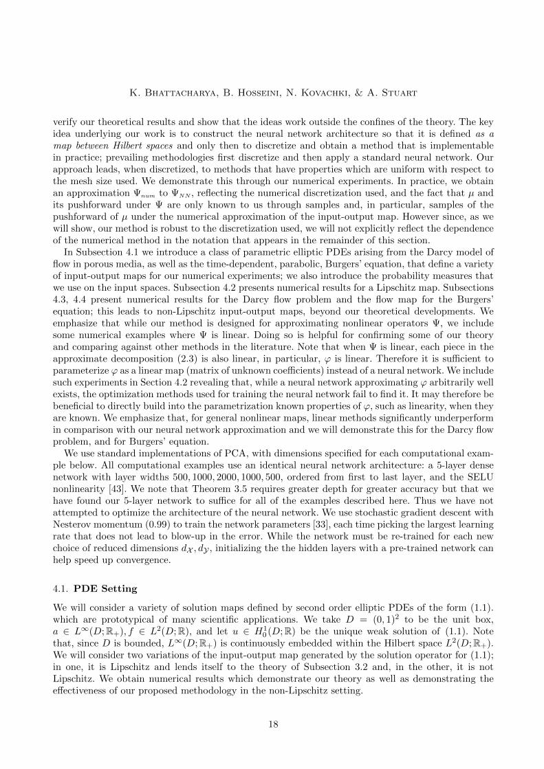
Figure 10. Relative test errors on both Darcy flow problems with reduced dimensiond = 70, training on a single mesh and transferring the solution to other meshes. Whenthe training mesh is smaller than the desired output mesh, the PCA basis are inter-polated using cubic splines. When the training mesh is larger than the desired outputmesh, the PCA basis are sub-sampled.

Figure 7 (a) shows the relative test errors as a function of the resolution when a ∼ µ = µL is log-normal while Figure 8 (a) shows them when a ∼ µ = µP is piecewise constant. In both settings, we seethat the error in our method is invariant to mesh-refinement. Since the problem is nonlinear, the neuralnetwork outperforms the linear map. However we see the same issue as in Figure 4 where increasingthe reduced dimension does not necessarily improve the error due to the increased complexity ofthe optimization problem. Panels (b) of Figures 7 and 8 confirm this observation. This issue can bealleviated with additional training data. Indeed, panels (c) of Figures 7 and 8 show that the error curveis flattened with more data. We highlight that these results are consistent with our interpretation ofTheorem 3.1: the reduced dimensions dX , dY are determined first by the properties of the measureµ and its pushforward, and then the amount of data necessary is obtained to ensure that the finitedata approximation error is of the same order of magnitude as the finite-dimensional approximationerror. In summary, the size of the training dataset N should increase with the number of reduceddimensions.

For this problem, we also compare to the reduced basis method (RB) when instantiated with PCA.We implement this by a standard Galerkin projection, expanding the solution in the PCA basis andusing the weak form of (1.1) to find the coefficients. We note that the errors of both methods arevery close, but we find that the online runtime of our method is significantly better. Letting K denotethe mesh-size and d the reduced dimension, the reduced basis method has a runtime of O(d2K + d3)while our method has the runtime O(dK) plus the runtime of the neural network which, in practice,we have found to be negligible. We show the online inference time as well as the offline training timeof the methods in Figure 9. While the neural network has the highest offline cost, its small onlinecost makes it a more practical method. Indeed, without parallelization when d = 150, the total time(online and offline) to compute all 5000 test solutions is around 28 hours for the RBM. On the otherhand, for the neural network, it is 28 minutes. The difference is pronounced when needing to computemany solutions in parallel. Since most modern architectures are able to internally parallelize matrix-matrix multiplication, the total time to train and compute the 5000 examples for the neural network is

24


(a) (b) (c)

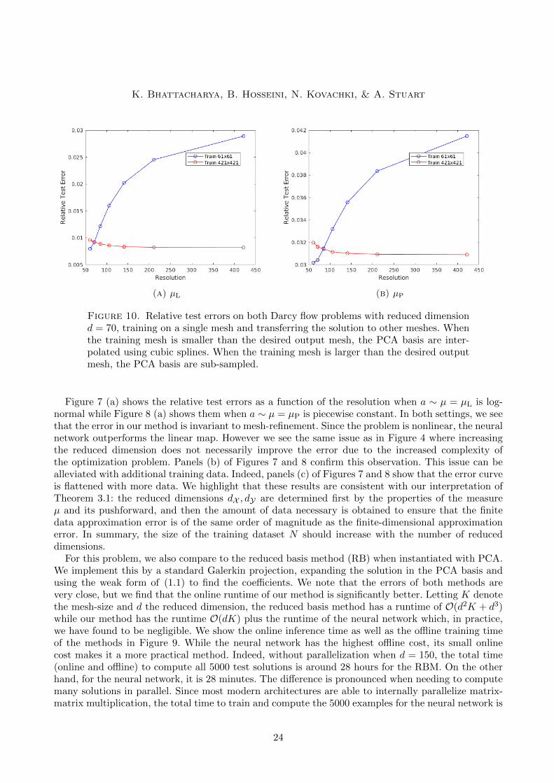
Figure 11. Relative test errors on the Burgers’ Equation problem. Using N = 1024training examples, panel (a) shows the errors as a function of the resolution while panel(b) fixes a 4096 mesh and shows the error as a function of the reduced dimension. Panel(c) only shows results for our method using a neural network, fixing a 4096 mesh andshowing the error as a function of the reduced dimension for different amounts oftraining data.

only 4 minutes. This issue can however be slightly alleviated for the reduced basis method with morestringent multi-core parallelization. We note that the linear map has the lowest online cost and only aslightly worse offline cost than the RBM. This makes it the most suitable method for linear operatorssuch as those presented in Section 4.2 or for applications where larger levels of approximation errorcan be tolerated.

We again note that the image-to-image regression approach of [83] does not scale with the meshsize. We do however acknowledge that for the small meshes for which the method was designed, it doesoutperform all other approaches. This begs the question of whether one can design neural networksthat match the performance of image-to-image regression but remain invariant with respect to thesize of the mesh. The contemporaneous work [51] takes a step in this direction.

Lastly, we show that our method also has the ability to transfer a solution learned on one meshto another. This is done by interpolating or sub-sampling both of the input and output PCA basisfrom the training mesh to the desired mesh. Justifying this requires a smoothness assumption on thePCA basis; we are, however, not aware of any such results and believe this is an interesting futuredirection. The neural network is fixed and does not need to be re-trained on a new mesh. We showthis in Figure 10 for both Darcy flow problems. We note that when training on a small mesh, the errorincreases as we move to larger meshes, reflecting the interpolation error of the basis. Nevertheless,this increase is rather small: as shown in Figure 10, we obtain a 3% and a 1% relative error increasingwhen transferring solutions trained on a 61×61 grid to a 421×421 grid on each respective Darcy flowproblem. On the other hand, when training on a large mesh, we see almost no error increase on thesmall meshes. This indicates that the neural network learns a property that is intrinsic to the solutionoperator and independent of the discretization.

4.4. Burgers’ Equation

We now consider the input-output map Ψ : L2(T1;R)→ Hr(T1;R) mapping u0 7→ u|t=1 in (4.1) withβ = 10−2 fixed. In this setting, Ψ is nonlinear and locally Lipschitz but since we do not know the preciseLipschitz constant as defined in Appendix A, we cannot verify that the assumptions of Theorem A.1hold; nevertheless the numerical results demonstrate the effectiveness of our methodology. We takeu0 ∼ µ = µB; see rows 5 of Figure 3 for an example. Figure 11 (a) shows the relative test errors as

25


a function of the resolution again demonstrating that our method is invariant to mesh-refinement.We note that, for this problem, the linear map does significantly worse than the neural network incontrast to the Darcy flow problem where the results were comparable. This is likely attributable tothe fact that the solution operator for Burgers’ equation is more strongly nonlinear. As before, weobserve from Figure 11 panel (b) that increasing the reduced dimension does not necessarily improvethe error due to the increased complexity of the optimization problem. This can again be mitigated byincreasing the volume of training data, as indicated in Figure 11(c); the curve of error versus reduceddimension is flattened as N increases.

5. Conclusion

In this paper, we proposed a general data-driven methodology that can be used to learn mappingsbetween separable Hilbert spaces. We proved consistency of the approach when instantiated with PCAin the setting of globally Lipschitz forward maps. We demonstrated the desired mesh-independentproperties of our approach on parametric PDE problems, showing good numerical performance evenon problems outside the scope of the theory.

This work leaves many interesting directions open for future research. To understand the interplaybetween the reduced dimension and the amount of data needed requires a deeper understanding ofneural networks and their interaction with the optimization algorithms used to produce the approx-imation architecture. Even if the optimal neural network is found by that optimization procedure,the question of the number of parameters needed to achieve a given level of accuracy, and how thisinteracts with the choice of reduced dimensions dX and dY (choice of which is determined by the inputspace probability measure), warrants analysis in order to reveal the computational complexity of theproposed approach. Furthermore, the use of PCA limits the scope of problems that can be addressedto Hilbert, rather than general Banach spaces; even in Hilbert space, PCA may not be the optimalchoice of dimension reduction. The development of autoenconders on function space is a promisingdirection that has the potential to address these issues; it also has many potential applications that arenot limited to deployment within the methodology proposed here. Finally we also wish to study theuse of our methodology in more challenging PDE problems, such as those arising in materials science,as well as for time-dependent problems such as multi-phase flow in porous media. Broadly speakingwe view our contribution as a first step in the development of methods that generalize the ideas andapplications of neural networks by operating on, and between, spaces of functions.

Acknowledgments

The authors are grateful to Anima Anandkumar, Kamyar Azizzadenesheli, Zongyi Li and Nicholas H.Nelsen for helpful discussions in the general area of neural networks for PDE-defined maps betweenHilbert spaces. The authors thank Matthew M. Dunlop for sharing his code for solving elliptic PDEsand generating Gaussian random fields. The work is supported by MEDE-ARL funding (W911NF-12-0022). AMS is also partially supported by NSF (DMS 1818977) and AFOSR (FA9550-17-1-0185). BHis partially supported by a Von Karman instructorship at the California Institute of Technology.

Bibliography

[1] Jonas Adler and Ozan Oktem. Solving ill-posed inverse problems using iterative deep neuralnetworks. Inverse Problems, nov 2017.

[2] BO Almroth, Perry Stern, and Frank A Brogan. Automatic choice of global shape functions instructural analysis. Aiaa Journal, 16(5):525–528, 1978.

26


[3] Maxime Barrault, Yvon Maday, Ngoc Cuong Nguyen, and Anthony T Patera. An ‘empiricalinterpolation’ method: application to efficient reduced-basis discretization of partial differentialequations. Comptes Rendus Mathematique, 339(9):667–672, 2004.

[4] Peter Baxendale. Gaussian measures on function spaces. American Journal of Mathematics,98(4):891–952, 1976.

[5] Mikhail Belkin and Partha Niyogi. Laplacian eigenmaps for dimensionality reduction and datarepresentation. Neural Computation, 15(6):1373–1396, 2003.

[6] Peter Benner, Pawan Goyal, Boris Kramer, Benjamin Peherstorfer, and Karen Willcox. Operatorinference for non-intrusive model reduction of systems with non-polynomial nonlinear terms.Computer Methods in Applied Mechanics and Engineering, 372:113433, Dec 2020.

[7] Saakaar Bhatnagar, Yaser Afshar, Shaowu Pan, Karthik Duraisamy, and Shailendra Kaushik. Pre-diction of aerodynamic flow fields using convolutional neural networks. Computational Mechanics,pages 1–21, 2019.

[8] Peter Binev, Albert Cohen, Wolfgang Dahmen, Ronald DeVore, Guergana Petrova, and Przemys-law Wojtaszczyk. Data assimilation in reduced modeling. SIAM/ASA Journal on UncertaintyQuantification, 5(1):1–29, 2017.

[9] Gilles Blanchard, Olivier Bousquet, and Laurent Zwald. Statistical properties of kernel principalcomponent analysis. Machine Learning, 66(2):259–294, Mar 2007.

[10] Sebastien Boyaval, Claude Le Bris, Tony Lelievre, Yvon Maday, Ngoc Cuong Nguyen, and An-thony T Patera. Reduced basis techniques for stochastic problems. Archives of Computationalmethods in Engineering, 17(4):435–454, 2010.

[11] Shengze Cai, Zhicheng Wang, Lu Lu, Tamer A Zaki, and George Em Karniadakis. Deepm&mnet:Inferring the electroconvection multiphysics fields based on operator approximation by neuralnetworks. arXiv preprint arXiv:2009.12935, 2020.

[12] Tianping Chen and Hong Chen. Universal approximation to nonlinear operators by neural net-works with arbitrary activation functions and its application to dynamical systems. IEEE Trans-actions on Neural Networks, 6(4):911–917, 1995.

[13] Lixue Cheng, Nikola B. Kovachki, Matthew Welborn, and Thomas F. Miller. Regression clusteringfor improved accuracy and training costs with molecular-orbital-based machine learning. Journalof Chemical Theory and Computation, 15(12):6668–6677, Dec 2019.

[14] Abdellah Chkifa, Albert Cohen, Ronald DeVore, and Christoph Schwab. Sparse adaptive Taylorapproximation algorithms for parametric and stochastic elliptic PDEs. ESAIM: MathematicalModelling and Numerical Analysis, 47(1):253–280, 2013.

[15] A Cohen, R DeVore, and C Scwhab. Analytic regularity and polynomial approximation of para-metric and stochastic elliptic PDEs. Analysis and Applications, 09(01):11–47, 2011.

[16] Albert Cohen, Wolfgang Dahmen, and Ron DeVore. State estimation–the role of reduced models.arXiv preprint:2002.00220, 2020.

[17] Albert Cohen and Ronald DeVore. Approximation of high-dimensional parametric pdes. ActaNumerica, 24:1–159, 2015.

27


[18] Albert Cohen, Ronald DeVore, and Christoph Schwab. Convergence rates of best n-term Galerkinapproximations for a class of elliptic SPDEs. Foundations of Computational Mathematics,10(6):615–646, 2010.

[19] R. R. Coifman, S. Lafon, A. B. Lee, M. Maggioni, B. Nadler, F. Warner, and S. W. Zucker.Geometric diffusions as a tool for harmonic analysis and structure definition of data: Diffusionmaps. Proceedings of the National Academy of Sciences, 102(21):7426–7431, 2005.

[20] M. Dashti, S. Harris, and A.M. Stuart. Besov priors for Bayesian inverse problems. Inverse Prob-lems and Imaging, 6:183–200, 2012.

[21] Ingrid Daubechies, Ronald A. DeVore, Simon Foucart, Boris Hanin, and Guergana Petrova. Non-linear approximation and (deep) ReLU networks. arXiv preprint:1905.02199, 2019.

[22] Ronald A. DeVore. Nonlinear approximation. Acta Numerica, 7:51–150, 1998.

[23] Ronald A. DeVore. The theoretical foundation of reduced basis methods. In Model Reduction andApproximation. SIAM, Philadelphia, 2014.

[24] Tim Dockhorn. A discussion on solving partial differential equations using neural networks. arXivpreprint:1904.07200, 2019.

[25] Weinan E and Bing Yu. The deep Ritz method: A deep learning-based numerical algorithm forsolving variational problems. Communications in Mathematics and Statistics, 3 2018.

[26] Lawrence C. Evans. Partial differential equations. American Mathematical Society, 2010.

[27] Ky Fan. On a theorem of Weyl concerning eigenvalues of linear transformations I. Proceedings ofthe National Academy of Sciences, 35(11):652–655, 1949.

[28] Stefania Fresca, Luca Dede, and Andrea Manzoni. A comprehensive deep learning-based ap-proach to reduced order modeling of nonlinear time-dependent parametrized pdes. arXiv preprintarXiv:2001.04001, 2020.

[29] Moritz Geist, Philipp Petersen, Mones Raslan, Reinhold Schneider, and Gitta Kutyniok. Nu-merical solution of the parametric diffusion equation by deep neural networks. arXiv preprintarXiv:2004.12131, 2020.

[30] Justin Gilmer, Samuel S Schoenholz, Patrick F Riley, Oriol Vinyals, and George E Dahl. Neuralmessage passing for quantum chemistry. In Proceedings of the 34th International Conference onMachine Learning, 2017.

[31] Francisco J Gonzalez and Maciej Balajewicz. Deep convolutional recurrent autoencoders for learn-ing low-dimensional feature dynamics of fluid systems. arXiv preprint arXiv:1808.01346, 2018.

[32] R Gonzalez-Garcia, R Rico-Martinez, and IG Kevrekidis. Identification of distributed parametersystems: A neural net based approach. Computers & chemical engineering, 22:S965–S968, 1998.

[33] Ian Goodfellow, Yoshua Bengio, and Aaron Courville. Deep Learning. MIT Press, 2016.

[34] Eldad Haber and Lars Ruthotto. Stable architectures for deep neural networks. Inverse Problems,34(1):014004, 2017.

28


[35] L Herrmann, Ch Schwab, and J Zech. Deep ReLU neural network expression rates for data-to-QoImaps in Bayesian PDE inversion. 2020.

[36] Jan S Hesthaven, Gianluigi Rozza, Benjamin Stamm, et al. Certified reduced basis methods forparametrized partial differential equations. SpringerBirefs In Mathematics. Springer, 2016.

[37] J.S. Hesthaven and S. Ubbiali. Non-intrusive reduced order modeling of nonlinear problems usingneural networks. Journal of Computational Physics, 363:55 – 78, 2018.

[38] Geoffrey Hinton and Ruslan Salakhutdinov. Reducing the dimensionality of data with neuralnetworks. Science, 313(5786):504 – 507, 2006.

[39] Jonathan R Holland, James D Baeder, and Karthikeyan Duraisamy. Field inversion and machinelearning with embedded neural networks: Physics-consistent neural network training. In AIAAAviation 2019 Forum, page 3200, 2019.

[40] Jun-Ting Hsieh, Shengjia Zhao, Stephan Eismann, Lucia Mirabella, and Stefano Ermon. Learn-ing neural PDE solvers with convergence guarantees. In International Conference on LearningRepresentations, 2019.

[41] M.A. Iglesias, K. Lin, and A.M. Stuart. Well-posed bayesian geometric inverse problems arisingin subsurface flow. Inverse Problems, 30:114001, 2014.

[42] Yuehaw Khoo, Jianfeng Lu, and Lexing Ying. Solving parametric pde problems with artificialneural networks. arXiv preprint arXiv:1707.03351, 2017.

[43] Gunter Klambauer, Thomas Unterthiner, Andreas Mayr, and Sepp Hochreiter. Self-normalizingneural networks. In I. Guyon, U. V. Luxburg, S. Bengio, H. Wallach, R. Fergus, S. Vishwanathan,and R. Garnett, editors, Advances in Neural Information Processing Systems 30, pages 971–980.Curran Associates, Inc., 2017.

[44] K Krischer, R Rico-Martınez, IG Kevrekidis, HH Rotermund, G Ertl, and JL Hudson. Modelidentification of a spatiotemporally varying catalytic reaction. AIChE Journal, 39(1):89–98, 1993.

[45] Gitta Kutyniok, Philipp Petersen, Mones Raslan, and Reinhold Schneider. A theoretical analysisof deep neural networks and parametric PDEs. 2019.

[46] Fabian Laakmann and Philipp Petersen. Efficient approximation of solutions of parametric lineartransport equations by relu dnns. arXiv preprint arXiv:2001.11441, 2020.

[47] Isaac E Lagaris, Aristidis Likas, and Dimitrios I Fotiadis. Artificial neural networks for solvingordinary and partial differential equations. IEEE transactions on neural networks, 9(5):987–1000,1998.

[48] Kody Law, Andrew Stuart, and Kostas Zygalakis. Data Assimilation: A Mathematical Introduc-tion, volume 62 of Texts in Applied Mathematics. Springer, 2015.

[49] Yann LeCun, Yoshua Bengio, and Geoffrey Hinton. Deep learning. Nature, 521(7553):436–444,May 2015.

[50] Kookjin Lee and Kevin T Carlberg. Model reduction of dynamical systems on nonlinear manifoldsusing deep convolutional autoencoders. Journal of Computational Physics, 404, 2020.

29


[51] Zongyi Li, Nikola Kovachki, Kamyar Azizzadenesheli, Burigede Liu, Kaushik Bhattacharya, An-drew Stuart, and Anima Anandkumar. Neural operator: Graph kernel networkfor partial differ-ential equations. arXiv preprint:2003.03485, 2020.

[52] Chensen Lin, Zhen Li, Lu Lu, Shengze Cai, Martin Maxey, and George Em Karniadakis. Operatorlearning for predicting multiscale bubble growth dynamics. arXiv preprint arXiv:2012.12816,2020.

[53] Gabriel J Lord, Catherine E Powell, and Tony Shardlow. An introduction to computational sto-chastic PDEs, volume 50. Cambridge University Press, 2014.

[54] Lu Lu, Pengzhan Jin, and George Em Karniadakis. Deeponet: Learning nonlinear operators foridentifying differential equations based on the universal approximation theorem of operators.arXiv preprint arXiv:1910.03193, 2019.

[55] Lu Lu, Pengzhan Jin, Guofei Pang, Zhongqiang Zhang, and George Em Karniadakis. Learningnonlinear operators via deeponet based on the universal approximation theorem of operators.Nature Machine Intelligence, 2020.

[56] Yvon Maday, Anthony T Patera, James D Penn, and Masayuki Yano. A parameterized-background data-weak approach to variational data assimilation: formulation, analysis, and appli-cation to acoustics. International Journal for Numerical Methods in Engineering, 102(5):933–965,2015.

[57] Vitaly Maiorov and Allan Pinkus. Lower bounds for approximation by MLP neural networks.Neurocomputing, 25:81–91, 1999.

[58] Zhiping Mao, Lu Lu, Olaf Marxen, Tamer A Zaki, and George E Karniadakis. Deepm&mnet forhypersonics: Predicting the coupled flow and finite-rate chemistry behind a normal shock usingneural-network approximation of operators. arXiv preprint arXiv:2011.03349, 2020.

[59] Shane A. McQuarrie, Cheng Huang, and Karen Willcox. Data-driven reduced-order models viaregularized operator inference for a single-injector combustion process, 2020.

[60] Kevin P. Murphy. Machine Learning: A Probabilistic Perspective. The MIT Press, 2012.

[61] Dennis A Nagy. Modal representation of geometrically nonlinear behavior by the finite elementmethod. Computers & Structures, 10(4):683–688, 1979.

[62] Michael L. Overton and Robert S. Womersley. On the sum of the largest eigenvalues of a sym-metric matrix. SIAM Journal of Matrix Analysis and Applications, 13(1):41–45, 1992.

[63] K. Pearson. LIII. On lines and planes of closest fit to systems of points in space. The London,Edinburgh, and Dublin Philosophical Magazine and Journal of Science, 2(11):559–572, 1901.

[64] Benjamin Peherstorfer. Sampling low-dimensional Markovian dynamics for pre-asymptoticallyrecovering reduced models from data with operator inference, 2019.

[65] Benjamin Peherstorfer and Karen Willcox. Data-driven operator inference for nonintrusiveprojection-based model reduction. Computer Methods in Applied Mechanics and Engineering,306:196 – 215, 2016.

30


[66] Elizabeth Qian, Boris Kramer, Benjamin Peherstorfer, and Karen Willcox. Lift & learn: Physics-informed machine learning for large-scale nonlinear dynamical systems. Physica D: NonlinearPhenomena, 406:132401, 2020.

[67] Alfio Quarteroni, Andrea Manzoni, and Federico Negri. Reduced basis methods for partial differ-ential equations: an introduction. Springer, 2015.

[68] Maziar Raissi, Paris Perdikaris, and George E Karniadakis. Physics-informed neural networks:A deep learning framework for solving forward and inverse problems involving nonlinear partialdifferential equations. Journal of Computational Physics, 378:686–707, 2019.

[69] Sebastian Reich and Colin Cotter. Probabilistic forecasting and Bayesian data assimilation. Cam-bridge University Press, 2015.

[70] Lars Ruthotto and Eldad Haber. Deep neural networks motivated by partial differential equations.Journal of Mathematical Imaging and Vision, 62:352 – 364, 2019.

[71] Christoph Schwab and Jakob Zech. Deep learning in high dimension: Neural network expressionrates for generalized polynomial chaos expansions in UQ. Analysis and Applications, 17(01):19–55,2019.

[72] B. Scholkopf, A. Smola, and K. Muller. Nonlinear component analysis as a kernel eigenvalueproblem. Neural Computation, 10(5):1299–1319, July 1998.

[73] J. Shawe-Taylor, C. K. I. Williams, N. Cristianini, and J. Kandola. On the eigenspectrum ofthe Gram matrix and the generalization error of kernel-PCA. IEEE Transactions on InformationTheory, 51(7):2510–2522, July 2005.

[74] John Shawe-Taylor, Chris Williams, Nello Cristianini, and Jaz Kandola. On the eigenspectrum ofthe Gram matrix and its relationship to the operator eigenspectrum. In International Conferenceon Algorithmic Learning Theory, pages 23–40. Springer, 2002.

[75] Yeonjong Shin, Jerome Darbon, and George Em Karniadakis. On the convergence and general-ization of physics informed neural networks. arXiv preprint arXiv:2004.01806, 2020.

[76] Jonathan D Smith, Kamyar Azizzadenesheli, and Zachary E Ross. Eikonet: Solving the eikonalequation with deep neural networks. arXiv preprint arXiv:2004.00361, 2020.

[77] Sin-Ei Takahasi, John M Rassias, Saburou Saitoh, and Yasuji Takahashi. Refined generalizationsof the triangle inequality on Banach spaces. Math. Inequal. Appl, 13(4):733–741, 2010.

[78] Roger Temam. Infinite-dimensional dynamical systems in mechanics and physics, volume 68.Springer Science & Business Media, 2012.

[79] Qian Wang, Jan S. Hesthaven, and Deep Ray. Non-intrusive reduced order modeling of unsteadyflows using artificial neural networks with application to a combustion problem. Journal of Com-putational Physics, 384:289 – 307, 2019.

[80] E Weinan. A proposal on machine learning via dynamical systems. Communications in Mathe-matics and Statistics, 5(1):1–11, 2017.

[81] Dmitry Yarotsky. Error bounds for approximations with deep ReLU networks. Neural Networks,94:103 – 114, 2017.

31


[82] Eberhard Zeidler. Applied Functional Analysis: Applications to Mathematical Physics. SpringerPublishing Company, Incorporated, 2012.

[83] Yinhao Zhu and Nicholas Zabaras. Bayesian deep convolutional encoder-decoder networks for sur-rogate modeling and uncertainty quantification. Journal of Computational Physics, 366(C):415–447, August 2018.

Appendix A. Neural Networks And Approximation (Locally Lipschitz Case)

This extends the approximation theory of Subsection 3.2 to the case of solution maps Ψ : X → Y thatare µ-measurable and locally Lipschitz in the following sense

∀x, z ∈ X ‖Ψ(x)−Ψ(z)‖Y ≤ L(x, z)‖x− z‖X . (A.1)

where the function L : X × X → R+ is symmetric in its arguments, i.e., L(x, z) = L(z, x), and forany fixed w ∈ X the function L(·, w) : X → R+ is µ-measurable and non-decreasing in the sense thatL(s, w) ≤ L(x,w) if ‖x‖X ≥ ‖w‖X . Note that this implies that Ψ is locally bounded: for any x ∈ X

‖Ψ(x)‖Y ≤ ‖Ψ(0)‖Y + ‖Ψ(x)−Ψ(0)‖Y ≤ ‖Ψ(0)‖Y + L(x, 0)‖x‖X .

Hence we deduce that the pushforward Ψ]µ has bounded fourth moments provided that Ex∼µ(L(x, 0)‖x‖X )4 <+∞:

Ey∼Ψ]µ‖y‖4Y =

∫X‖Ψ(x)‖4Ydµ(x) ≤

∫X

(‖Ψ(0)‖Y + L(x, 0)‖x‖X )4dµ(x)

≤ 23

(‖Ψ(0)‖Y +

∫XL(x, 0)4‖x‖4Xdµ(x)

)<∞,

where we used a generalized triangle inequality proven in [77, Cor. 3.1].

Theorem A.1. Let X , Y be real, separable Hilbert spaces, Ψ a mapping from X into Y and let µ bea probability measure supported on X such that

Ex∼µL(x, x)2 < +∞, Ex∼µL(x, 0)2‖x‖2X <∞,

where L(·, ·) is given in (A.1). Fix dX , dY , N ≥ maxdX , dY, δ ∈ (0, 1), τ > 0 and define M =√Ex∼µ‖x‖2X /δ. Then there exists a constant c(dX , dY) ≥ 0 and neural network χ ∈M(dX , dY ; t, r,M)

with t ≤ c(log(√dY/τ) + 1) layers and r ≤ c(ε−dX log(

√dY/τ) + 1) active weights and biases in each

component, so that

Exj∼µEx∼µ(eNN(x)

)≤ C

(τ +√δ

+

(√dXN

+Rµ(V XdX )

)1/2

+

(√dYN

+RΨ]µ(V YdY )

)1/2),

(A.2)

where eNN(x) := ‖ΨNN(x)−Ψ(x)‖Y and C > 0 is independent of dX , dY , N, δ and ε.

Proof. Our method of proof is similar to the proof of Theorem 3.5 and for this reason we shortensome of the arguments. Recall the constant Q from Theorem 3.4. In what follows we take Q to bethe maximum of the two such constants when arising from application of the theorem on the twodifferent probability spaces (X , µ) and (Y,Ψ]µ). As usual we employ the shorthand notation E to

denote Exj∼µ the expectation with respect to the dataset xjNj=1.

32


We begin by approximating the error incurred by using ΨPCA given by (2.3):

EEx∼µ‖ΨPCA(x)−Ψ(x)‖Y = EEx∼µ‖(GY FY Ψ GX FX )(x)−Ψ(x)‖Y

= EEx∼µ∥∥∥∥ΠV Y

dY ,NΨ(ΠV X

dX ,Nx)−Ψ(x)

∥∥∥∥Y

≤ EEx∼µ∥∥∥∥ΠV Y

dY ,NΨ(ΠV X

dX ,Nx)−ΠV Y

dY ,NΨ(x)

∥∥∥∥Y

+ EEx∼µ∥∥∥∥ΠV Y

dY ,NΨ(x)−Ψ(x)

∥∥∥∥Y

≤ EEx∼µL(ΠV XdX ,N

x, x)∥∥∥ΠV X

dX ,Nx− x

∥∥∥X

+ EEy∼Ψ]µ


y − y∥∥∥∥Y,

(A.3)

noting that the operator norm of an orthogonal projection is 1. Now since L(·, x) is non-decreasing weinfer that L(ΠV X

dX ,Nx, x) ≤ L(x, x) and then using Cauchy-Schwarz we obtain

EEx∼µ‖ΨPCA(x)−Ψ(x)‖Y ≤(Ex∼µ|L(x, x)|2

)1/2(EEx∼µ ∥∥∥ΠV XdX ,N

x− x∥∥∥2

X

)1/2

+ EEy∼Ψ]µ


y − y∥∥∥∥Y,

= L′(ERµ(V XdX ,N )

)1/2+(E[RΨ]µ(V YdY ,N )]

)1/2

(A.4)

where we used Holder’s inequality in the last line and defined the new constant L′ :=(Ex∼µ|L(x, x)|2

)1/2.

Theorem 3.4 allows us to control this error, and leads toEEx∼µeNN ≤ EEx∼µ‖ΨNN(x)−ΨPCA(x)‖Y + EEx∼µ‖ΨPCA(x)−Ψ(x)‖Y

≤ Ex∼µ‖ΨNN(x)−ΨPCA(x)‖Y

+ L′

(√QdXN

+Rµ(V XdX )

)1/2

+

(√QdYN

+RΨ]µ(V YdY )

)1/2

.

(A.5)

We now approximate ϕ by a neural network χ as before. To that end we first note from LemmaB.3 that ϕ is locally Lipschitz, and hence continuous, as a mapping from RdX into RdY . Identify thecomponents ϕ(s) = (ϕ(1)(s), . . . , ϕ(dY )(s)) where each function ϕ(j) ∈ C(RdX ;R). We consider therestriction of each component function to the set [−M,M ]dX .By [81, Thm. 1] and using the same arguments as in the proof of Theorem 3.5 there exist neural

networks χ(1), . . . , χ(dY ) : RdX → R, χ(j) ∈ M(dX ; t(j), r(j)), with layer and active weight parameters

t(j) and r(j) satisfying t(j) ≤ c(j)[log(M√dY/τ) + 1], and r(j) ≤ c(j)(τ/2M)−dX [log(M

√dY/τ) + 1]

with constants c(j)(dX ) > 0, so that∣∣(χ(1)(s), . . . , χ(dY )(s))− ϕ(s)

∣∣2< τ ∀s ∈ [−M,M ]dX .

We now simply define χ : RdX → RdY as the stacked network (χ(1), . . . , χdY ) extended by zero outsideof [−M,M ]dX to immediately obtain

sups∈[−M,M ]dX

∣∣χ(s)− ϕ(s)∣∣2< τ. (A.6)

Thus, by construction χ ∈ M(dX , dY , t, r,M) with at most t ≤ maxj t(j) many layers and r ≤ r(j)

many active weights and biases in each of its components.Define the set A = x ∈ X : FX (x) ∈ [−M,M ]dX . By Lemma B.4 below, µ(A) ≥ 1−δ and µ(Ac) ≤ δ.Define the approximation error ePCA(x) := ‖ΨNN(x)−ΨPCA(x)‖Y and decompose its expectation as

Ex∼µ[ePCA(x)] =

∫AePCA(x)dµ(x) +

∫Ac

ePCA(x)dµ(x) =: IA + IAc .

33


For the first term,

IA ≤∫A‖(GY χ FX )(x)− (GY ϕ FX )(x)‖Ydµ(x) ≤ τ, (A.7)

by using the fact, established in Lemma B.3, that GY is Lipschitz with Lipschitz constant 1, theτ -closeness of χ to ϕ from (A.6), and µ(A) ≤ 1. For the second term we have, using that GY hasLipschitz constant 1 and that χ takes value zero on Ac,

IAc ≤∫Ac

‖(GY χ FX )(x)− (GY ϕ FX )(x)‖Ydµ(x)

≤∫Ac

|χ(FX (x))− ϕ(FX (x))|2dµ(x) =

∫Ac

|ϕ(FX (x))|2dµ(x).

(A.8)

Once more from Lemma B.3 we have that

|FX (x)|2 ≤ ‖x‖X ; |ϕ(v)|2 ≤ |ϕ(0)|2 + L(GX (v), 0)|v|2so that, using the hypothesis on L and global Lipschitz property of FX and GX we can write

IAc ≤ µ(Ac)|ϕ(0)|2 +

∫Ac

L(x, 0)|FX (x)|2dµ(x)

≤ µ(Ac)|ϕ(0)|2 +

∫Ac

L(x, 0)‖x‖Xdµ(x)

≤ µ(Ac)|ϕ(0)|2 + µ(Ac)12(Ex∼µL(x, 0)2‖x‖2X

)1/2≤ δ|ϕ(0)|2 + δ

12L′′

≤√δ(|ϕ(0)|2 + L′′)

(A.9)

where L′′ :=(Ex∼µL(x, 0)2‖x‖2X

)1/2. Combining (3.3), (3.5) and (3.7) we obtain the desired result.

Appendix B. Supporting Lemmas

In this Subsection we present and prove auxiliary lemmas that are used throughout the proofs in thearticle. The proof of Theorem 3.4 made use of the following proposition, known as Fan’s Theorem,proved originally in [27]. We state and prove it here in the infinite-dimensional setting as this gen-eralization may be of independent interest. Our proof follows the steps of Fan’s original proof in thefinite-dimensional setting. The work [62], through which we first became aware of Fan’s result, givesan elegant generalization; however it is unclear whether that approach is easily applicable in infinitedimensions due to issues of compactness.

Lemma B.1 (Fan [27]). Let (H, 〈·, ·〉, ‖·‖) be a separable Hilbert space and C : H → H a non-negative,self-adjoint, compact operator. Denote by λ1 ≥ λ2 ≥ . . . the eigenvalues of C and, for any d ∈ N\0,let Sd denote the set of collections of d orthonormal elements of H. Then

d∑j=1

λj = maxu1,...,ud∈Sd

d∑j=1

〈Cuj , uj〉.

Proof. Let φ1, φ2, . . . denote the orthonormal eigenfunctions of C corresponding to the eigenvaluesλ1, λ2, . . . respectively. Note that for φ1, . . . , φd ∈ Sd, we have

d∑j=1

〈Cφj , φj〉 =

d∑j=1

λj‖φj‖2 =

d∑j=1

λj .

34


Now let u1, . . . , ud ∈ Sd be arbitrary. Then for any j ∈ 1, . . . , d, we have uj =∑∞

k=1〈uj , φk〉φkand thus

〈Cuj , uj〉 =∞∑k=1

λk|〈uj , φk〉|2

= λd

∞∑k=1

|〈uj , φk〉|2 +∞∑

k=d+1

(λk − λd)|〈uj , φk〉|2 +d∑

k=1

(λk − λd)|〈uj , φk〉|2.

Since ‖uj‖2 = 1, we have ‖uj‖2 =∑∞

k=1 |〈uj , φk〉|2 = 1 therefore

λd

∞∑k=1

|〈uj , φk〉|2 +∞∑

k=d+1

(λk − λd)|〈uj , φk〉|2 = λd

d∑k=1

|〈uj , φk〉|2 +∞∑

k=d+1

λk|〈uj , φk〉|2

≤ λd∞∑k=1

|〈uj , φk〉|2 = λd

using the fact that λk ≤ λd, ∀k > d. We have shown 〈Cuj , uj〉 ≤ λd +∑d

k=1(λk − λd)|〈uj , φk〉|2. Thusd∑j=1

(λj − 〈Cuj , uj〉) ≥d∑j=1

(λj − λd −

d∑k=1

(λk − λd)|〈uj , φk〉|2)

=d∑j=1

(λj − λd)

(1−

d∑k=1

|〈uk, φj〉|2).

We now extend the finite set of ukdk=1 from a d−dimensional orthonormal set to an orthonormalbasis uk∞k=1 for H. Note that λj ≥ λd, ∀j ≤ d and that

d∑k=1

|〈uk, φj〉|2 ≤∞∑k=1

|〈uk, φj〉|2 = ‖φj‖2 = 1

therefore∑d

j=1(λj − 〈Cuj , uj〉) ≥ 0 concluding the proof.

Theorem 3.4 relies on a Monte Carlo estimate of the Hilbert-Schmidt distance between C and CNthat we state and prove below.

Lemma B.2. Let C be given by (2.12) and CN by (2.6) then there exists a constant Q ≥ 0, dependingonly on ν, such that

Euj∼ν‖CN − C‖2HS =

Q

N.

Proof. Define C(uj) := uj ⊗ uj for any j ∈ 1, . . . , N and C(u) := u⊗ u for any u ∈ H, noting that

Eu∼ν [C(u)] = C = Euj∼ν [C(uj)]. Further we note that

Eu∼ν‖C(u)‖2HS = Eu∼ν‖u‖4 <∞

35


and, by Jensen’s inequality, ‖C‖2HS ≤ Eu∼ν‖C(u)‖2HS <∞. Once again using the shorthand notationE in place of Euj∼ν we compute,

E‖CN − C‖2HS = E‖ 1

N

N∑j=1

C(uj) − C‖2HS = E‖ 1

N

N∑j=1

C(uj)‖2HS − ‖C‖2HS

=1

NEu∼ν‖C(u)‖2HS +

1

N2

N∑j=1

N∑k 6=j〈E[C(uj)],E[C(uk)]〉HS − ‖C‖2HS

=1

NEu∼ν‖C(u)‖2HS +

N2 −NN2

‖C‖2HS − ‖C‖2HS

=1

N

(Eu∼ν‖C(u)‖2HS − ‖C‖2HS

)=

1

NEu∼ν‖C(u) − C‖2HS .

Setting Q = Eu∼ν‖C(u) − C‖2HS completes the proof.

The following lemma, used in the proof of Theorem 3.5, estimates Lipschitz constants of variousmaps required in the proof.

Lemma B.3. The maps FX , FY , GX and GY are globally Lipschitz:

|FX (v)− FX (z)|2 ≤ ‖v − z‖X , ∀v, z ∈ X|FY(v)− FY(v)|2 ≤ ‖v − z‖Y , ∀v, z ∈ Y

‖GX (v)−GX (z)‖X ≤ |v − z|2, ∀v, z ∈ RdX

‖GY(v)−GY(z)‖X ≤ |v − z|2, ∀v, z ∈ RdY .Furthermore, if Ψ is locally Lipschitz and satisfies

∀x,w ∈ X ‖Ψ(x)−Ψ(w)‖Y ≤ L(x,w)‖x− w‖X ,with L : X × X → R+ that is symmetric with respect to its arguments, and increasing in the sensethat L(s, w) ≤ L(x,w), if ‖x‖X ≥ ‖s‖X . Then ϕ is also locally Lipschitz and

|ϕ(v)− ϕ(z)|2 ≤ L(GX (v), GX (z))|v − z|2, ∀v, z ∈ RdX .

Proof. We establish that FY and GX are Lipschitz and estimate the Lipschitz constants; the proofsfor FX and GY are similar. Let φY1,N , . . . , φ

YdY ,N

denote the eigenvectors of the empirical covariance

with respect to the data yjNj=1 which span V YdY ,N and let φYdY+1,N , φYdY+2,N , . . . be an orthonormal

extension to Y. Then, by Parseval’s identity,

|FY(v)− FY(z)|22 =

dY∑j=1

〈v − z, φYj,N 〉2Y ≤

∞∑j=1

〈v − z, φYj,N 〉2Y = ‖v − z‖2Y .

A similar calculation for GX , using φX1,N , . . . , φXdX ,N

the eigenvectors of the empirical covariance of the

data xjNj=1 yields

‖GX (v)−GX (z)‖2X = ‖dX∑j=1

(vj − zj)φXj,N‖2X =

dX∑j=1

|vj − zj |2 = |v − z|22

for any v, z ∈ RdX , using the fact that the empirical eigenvectors can be extended to an orthonormalbasis for X . Recalling that ϕ = FY Ψ GX , the above estimates immediately yield

|ϕ(v)− ϕ(z)|2 ≤ L(GX (v), GX (z))|v − z|2, ∀v, z ∈ RdX .

36


The following lemma establishes a bound on the size of the set A that was defined in the proof ofTheorems 3.5 and A.1.

Lemma B.4. Fix 0 < δ < 1, let x ∼ µ be a random variable and set M =√Ex∼µ‖x‖2X /δ. Define FX

using the random dataset xjNj=1 ∼ µ then,

P(FX (x) 6∈ [−M,M ]dX

)≤ δ,

where the probability is computed with respect to both x and the xj’s.

Proof. Denote by φX1,N , . . . , φXdX ,N

the orthonormal set used to define V XdX ,N (2.7) and let φXdX +1,N , φXdX +2,N , . . .

be an orthonormal extension of this basis to X . For any j ∈ 1, . . . , dX , by Chebyshev’s inequality,we have

Px∼µ(|〈x, φXj,N 〉X | ≥M) ≤Ex∼µ|〈x, φXj,N 〉X |2

M2.

Note that the expectation is taken only with respect to the randomness in x and not φX1,N , . . . , φXdX ,N

,so the right hand side is itself a random variable. We further compute

Px∼µ(|〈x, φX1,N 〉X | ≥M, . . . , |〈x, φXdX ,N 〉X | ≥M)

≤ 1

M2Ex∼µ

dX∑j=1

|〈x, φXj,N 〉X |2 ≤1

M2Ex∼µ

∞∑j=1

|〈x, φXj,N 〉X |2 =1

M2Ex∼µ‖x‖2X

noting that ‖x‖2X =∑∞

j=1 |〈x, ξj〉X |2 for any orthonormal basis ξj∞j=1 of X hence the randomness in

φX1,N , φX2,N , . . . is inconsequential. Thus we find that, with P denoting probability with respect to both

x ∼ µ and the random data used to define FX ,

P(|〈x, φX1,N 〉X | ≤M, . . . , |〈x, φXdX ,N 〉X | ≤M) ≥ 1− 1

M2Ex∼µ‖x‖2X ,= 1− δ

the desired result.

Appendix C. Analyticity of the Poisson Solution Operator

Define X = ξ ∈ `∞(N;R) : ‖ξ‖`∞ ≤ 1 and let φj∞j=1 be some sequence of functions with the

property that (‖φj‖L∞)j≥1 ∈ `p(N;R) for some p ∈ (0, 1). Define Ψ : X → H10 (D;R) as mapping a set

of coefficients ξ = (ξ1, ξ2, . . . ) ∈ X to u ∈ H10 (D;R) the unique weak solution of

−∆u =

∞∑j=1

ξjφj in D, u|∂D = 0.

Note that since D is a bounded domain and ξ ∈ X , we have that∑∞

j=1 ξjφj ∈ L2(Ω;R) since our

assumption implies (‖φj‖L∞)j≥1 ∈ `1(N;R). Therefore u is indeed the unique weak-solution of thePoisson equation [26, Chap. 6] and Ψ is well-defined.

Theorem C.1. Suppose that there exists p ∈ (0, 1) such that (‖φj‖L∞)j≥1 ∈ `p(N;R). Then

limK→∞

supξ∈X‖Ψ(ξ)−

K∑j=1

ξjηj‖H10

= 0

where, for each j ∈ N, ηj ∈ H10 (D;R) satisfies

−∆ηj = φj in D, u|∂D = 0.

37


Proof. By linearity and Poincare inequality, we obtain the Lipschitz estimate

‖Ψ(ξ(1))−Ψ(ξ(2))‖H10≤ C‖

∞∑j=1

(ξ(1)j − ξ

(2)j )φj‖L2 , ∀ξ(1), ξ(2) ∈ X

for some C > 0. Now let ξ = (ξ1, ξ2, . . . ) ∈ X be arbitrary and define the sequence ξ(1) = (ξ1, 0, 0, . . . ), ξ(2) =

(ξ1, ξ2, 0, . . . ), . . .. Note that, by linearity, for any K ∈ N, Ψ(ξ(K)) =∑K

j=1 ξjηj . Then, using our Lips-chitz estimate,

‖Ψ(ξ)−Ψ(ξK)‖H10. ‖

∞∑j=K+1

ξjφj‖L2 .∞∑

j=K+1

‖φj‖L∞ ≤ K1− 1p ‖(‖φj‖L∞)j≥1‖`p

where the last line follows by Stechkin’s inequality [15, Sec. 3.3]. Taking the supremum over ξ ∈ Xand the limit K →∞ completes the proof.

Appendix D. Error During Training

Figures 12 and 13 show the relative test error computed during the training process for the problemspresented in Section 4.2. For both problems, we observe a slight amount of overfitting when moretraining samples are used and the reduced dimension is sufficiently large. This is because the truemap of interest ϕ is linear while the neural network parameterization is highly non-linear hence moreprone to overfitting larger amounts of data. While this suggests that simpler neural networks mightperform better on this problem, we do not carry out such experiments as our goal is simply to showthat building in a priori information about the problem (here linearity) can be beneficial as show inFigures 4 and 5.

(a) N = 1000 (b) N = 2000 (c) N = 4000 (d) N = 5000

Figure 12. Relative test errors as a function of the training epoch on the linear ellipticproblem. The amount of training examples used is varied in each panel.

38


(a) N = 1000 (b) N = 2000 (c) N = 4000 (d) N = 5000

Figure 13. Relative test errors as a function of the training epoch on the Poissonproblem. The amount of training examples used is varied in each panel.

39

model reduction and neural networks for parametric pdes

Documents