model order reduction of aeroservoelastic model of ... institute of aeronautics and astronautics 1...

American Institute of Aeronautics and Astronautics

1

Model Order Reduction of Aeroservoelastic Model of Flexible Aircraft

Yi Wang1, Hongjun Song2, Kapil Pant 3

CFD Research Corporation, Huntsville, AL 35806

and

Martin J. Brenner4, Peter Suh5

NASA Armstrong Flight Research Center, Edwards, CA 93523

This paper presents a holistic model order reduction (MOR) methodology and

framework that integrates key technological elements of sequential model reduction,

consistent model representation, and model interpolation for constructing high-quality

linear parameter-varying (LPV) aeroservoelastic (ASE) reduced order models (ROMs) of

flexible aircraft. The sequential MOR encapsulates a suite of reduction techniques, such as

truncation and residualization, modal reduction, and balanced realization and truncation to

achieve optimal ROMs at grid points across the flight envelope. The consistence in state

representation among local ROMs is obtained by the novel method of common subspace

reprojection. Model interpolation is then exploited to stitch ROMs at grid points to build a

global LPV ASE ROM feasible to arbitrary flight condition. The MOR method is applied to

the X-56A MUTT vehicle with flexible wing being tested at NASA/AFRC for flutter

suppression and gust load alleviation. Our studies demonstrated that relative to the full-

order model, our X-56A ROM can accurately and reliably capture vehicles dynamics at

various flight conditions in the target frequency regime while the number of states in ROM

can be reduced by 10X (from 180 to 19), and hence, holds great promise for robust ASE

controller synthesis and novel vehicle design.

Nomenclature

A = state matrix

Am = state matrix in the modal form

B = input matrix

C = output state matrix

D = input transition

L̂ = accumulative transformation matrix

M = matrices in state space model

P = controllability gramian

p = pitch rate

Q = observability gramian

q = pitch rate

R = common subspace for reprojection

r = yaw rate

T = transformation matrix for consistent state representation

L̂ = accumulative transformation matrix

u = input signals

y = response measurements

V = transformation matrix in balanced realization

1 Director, CFD Research Corporation, AIAA Member; [email protected] 2 Principal Research Engineer, CFD Research Corporation, non AIAA Member; [email protected] 3 Vice President, CFD Research Corporation, non AIAA Member; [email protected] 4 Aerospace Engineer, Aerostructures Branch, and AIAA Senior Member; [email protected] 5 Aerospace Engineer, Aerostructures Branch, and AIAA Member; [email protected]

https://ntrs.nasa.gov/search.jsp?R=20160000869 2018-07-07T06:18:13+00:00Z


2

W = transformation matrix in balanced realization

W = weights for matrix interpolation

= a vector of measurable parameters

= diagonal blocks of the eigenvalue magnitude in the modal form

= Matrix for modal form transformation

I. Introduction

he flight performance of aerospace systems is characterized by the interaction between aerodynamics, structural

dynamics, and flight control dynamics. Modern designs of aerospace vehicles utilize state-of-the-art materials

and flexible structures that are lightweight and low-cost to achieve better maneuverability, and high performance. As

the structures become progressively lighter and more flexible, they are prone to complex dynamics, stability and

durability issues. In addition, the control systems interactions with aerodynamic and structural nonlinearities can

result in instabilities such as flutter [1], limit cycle oscillations (LCO) [2], and gust loads [3], leading to

unacceptable flight conditions and risk to the mission. Modeling, and especially maneuvering simulation, of high-

order aeroservoelastic (ASE) systems is essential for successful development of relatively lightweight, necessarily

flexible, aircraft with complex unsteady and often nonlinear aerodynamics. Therefore, the ability to accurately

predict aeroelastic (AE) behavior in conjunction with control law design of sensors and actuators is essential for

developing high-performance, safe aerospace vehicles. Although high-fidelity simulation coupling the nonlinear

aerodynamics with structural models enables a direct insight into the aforementioned phenomena, its prohibitive

computational cost, speed mismatch, nonlinear nature, as well as difficulty to deploy controllers with high-state-

order models render it impractical for integration in the design environment involving concurrent ASE analysis and

control synthesis and design.

To address these challenges, a variety of model order reduction (MOR) techniques have been developed in

conjunction with the linear parameter varying (LPV) formulation to reduce high-order aircraft ASE model into a

reduced state-space form while retaining dominant dynamics of the system. In LPV, the fully coupled nonlinear

aircraft model is represented as an ensemble of linear models of which the system parameters vary across the flight

regime. The landmark efforts in the area include regular truncation and residualization [4], modal reduction [5],

balanced realization and truncation [4, 5], Krylov-based projection and the hybrid SVD-Krylov approach [6]. MOR

approaches based on model transformation and truncation, such as modal reduction, balanced realization, and

Krylov projection lead to different state representation of the reduced models at various parameter locations in the

flight envelope, and hence, they cannot be immediately interpolated. In order to interpolate reduced models to form

global LPV models encompassing the entire flight envelope, various model transformation techniques have been

proposed to achieve consistent state representation among local reduced models prior to interpolation. Hjartarson et

al. [4] developed an LPV aeroservoelastic control toolbox (LPVtools), which was used to derive the reduced state-

space form of a grid-based LPV model of aircraft. In their approach, the transformation matrix obtained from

balanced realization at a single flight condition was applied across the entire flight envelope to preserve consistent

state presentation (but at the cost of non-optimal reduction performance). Moreno et al [7] exploited the coprime

factorization approach in conjunction with the balanced realization to attain a low-order, control-oriented LPV Body

Freedom Flutter (BFF) model with 26 states consistent across the flight domain, and identify the numerical issues of

the approach associated with the high state orders. Panzer et al. [8] proposed two methods, respectively, based on

reprojection into a common subspace and optimization-based matrix matching to achieve identical state meanings

among local models for interpolation. The former was employed for interpolating LPV reduced models of industrial

flexible aircraft [6]. Recently Theis et al [5] developed another modal matching technique, which essentially

determines a mode-wise canonical form and matches modes with similar dynamic properties at neighboring grid

points to minimize the approximation error due to state inconsistency.

This paper presents the development of LPV ASE reduced order models (ROMs) of flexible aircrafts based on a

combination of sequential model order reduction (MOR), consistent model representation, and model interpolation

approaches. The sequential MOR encapsulates a suite of reduction techniques, such as traditional truncation and

residualization, modal reduction, and balanced realization and truncation, and is applied to the X-56A MUTT

vehicle with flexible wing developed by Lockheed Martin and currently being tested at NASA/AFRC for flutter

suppression and gust load alleviation. The traditional truncation and residualization methods are first conducted on

the states of the sensors, actuators, aerodynamic lags, rigid bodies, elastic structures of the full-order X-56A MUTT

ASE model sequentially. The transformation-based MOR including modal reduction and balanced realization and

truncation is then performed to further refine the frequency contents and remove the states with small contribution to

the input/output energy of the system in the local reduced model. Next, the method of reprojection into a common

T


3

subspace is utilized to remedy the issue of inconsistent state representation among the local reduced models caused

by the flight condition-dependent transformation above, which allows model interpolation in the reduced domain

and results in a unified LPV ROM applicable across the entire flight envelope. The input/output behavior and the

system response of the original and the ASE ROMs of the X-56A is compared in the frequency domain.

II. Linear Parameter-Varying Aeroservoelastic Models of Aircraft

Linear parameter-varying (LPV) models are state-space models whose state-space descriptions are functions of

time-varying parameters, i.e.,

A B x tx

C D u ty

(1)

where A() is the state matrix, B() is the input matrix, C() is the output state matrix, D() is the input transition

matrix, np is a vector of measurable parameters (such as altitude, Mach, fuel weight, etc.), unu and yny

are, respectively the vector of the control input and measurement. There are several methods to represent the

parameter dependence in LPV models above, such as linear fractional transformation, polytopic dependence of the

state matrix on the parameters, linearization on a gridded domain, etc. This paper targets the MOR of LPV models

based on the gridded domain to agree with the full-order X-56A models. The gridded domain LPV is illustrated in

Figure 1, in which the nonlinear dynamics in the ASE problem of the aircraft is treated as its linearization around

various flight operating points (also termed grid points or parameter locations hereafter). A set of original, full-order

Linear Time Invariant (LTI) state space models are first constructed at the grid points in the domain, and then can be

used for ROM generation and controller synthesis.

Figure 1. linear parameter varying (LPV) formulation of the aeroservoelastic (ASE) models of aircraft

III. Model Order Reduction for LPV Aircraft Models

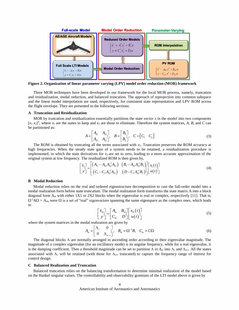
Figure 2 illustrates our MOR methodology for LPV ASE models of aircraft. A prerequisite of the approach to

construct LPV ROMs is to first have a set of full-order LTI state space models describing coupled ASE and flight

control behavior at grid points in the parameter space. The full model can be generated from various relevant

modeling tools (e.g., ZAERO [9], NASTRAN [10] or others) as shown in the blue box in Figure 2a. The entire

MOR process includes two steps: (1) Local MOR (red box in Figure 2a): the full-order LTI model set is first

reduced and transformed onto a low-dimension subspace to generate a set of local ROMs. Several techniques can be

used, including truncation and residualization, transformation and truncation (e.g., modal reduction and balanced

realization and truncation, Krylov methods, and their combinations); and (2) Model Interpolation and PV ROM

Realization (green box): the global LPV ROM applicable to the entire flight envelope is obtained by interpolating

the system matrices of the local ROM set obtained in the previous step. As the transformation used in step (1)

depends on the location of the grid points, measures need to be taken to ensure all the ROMs are cast in a consistent

state representation (or coordinates) prior to model interpolation. Eq. (2) summarizes the MOR process

* ** ** ** *

MOR

*ConsistentState *Represenation

Parameter

i i PV PVi Varyingi ii

i i PV pVi i

A B x t A Bx x xA Bx x

C D u t C Dy u t u tC Dy y

(2)


4

Figure 2. Organization of linear parameter varying (LPV) model order reduction (MOR) framework

Three MOR techniques have been developed in our framework for the local MOR process, namely, truncation

and residualization, modal reduction, and balanced truncation. The approach of reprojection into common subspace

and the linear model interpolation are used, respectively, for consistent state representation and LPV ROM across

the flight envelope. They are presented in the following sections:

A Truncation and Residualization

MOR by truncation and residualization essentially partitions the state vector x in the model into two components

[x1 x2]T, where x1 are the states to keep and x2 are those to eliminate. Therefore the system matrices, A, B, and C can

be partitioned as:

11 12 1

1 2

21 22 2

, ,A A B

A B C C CA A B

(3)

The ROM is obtained by truncating all the terms associated with x2. Truncation preserves the ROM accuracy at

high frequencies. When the steady state gain of a system needs to be retained, a residualization procedure is

implemented, in which the state derivatives for x2 are set to zero, leading to a more accurate approximation of the

original system at low frequency. The residualized ROM is then given by,

1 1

11 12 22 21 1 12 22 2 11

1 1

1 2 22 21 2 22 2

A A A A B A A B x tx

u ty C C A A D C A B

(4)

B Modal Reduction

Modal reduction relies on the real and ordered eigenstructure decomposition to cast the full-order model into a

modal realization form before state truncation. The modal realization form transforms the state matrix A into a block

diagonal form Am with either 1X1 or 2X2 blocks when the eigenvalue is real or complex, respectively [11]. That is,

-1A = Am, were is a set of “real” eigenvectors spanning the same eigenspace as the complex ones, which leads

to

m m mm

m

A B x tx

C D u ty

(5)

where the system matrices in the modal realization are given by

1

0, ,

0

r

m m m

n r

A B B C C

(6)

The diagonal blocks are normally arranged in ascending order according to their eigenvalue magnitude. The

magnitude of a complex eigenvalue (for an oscillatory mode) is its angular frequency, while for a real eigenvalue, it

is the damping coefficient. Then a threshold magnitude can be set to partition in Am into r and n-r. All the states

associated with r will be retained (with those for n-r truncated) to capture the frequency range of interest for

control design.

C Balanced Realization and Truncation

Balanced truncation relies on the balancing transformation to determine minimal realization of the model based

on the Hankel singular values. The controllability and observability gramians of the LTI model above is given by


5

0 and 0T T T TAP PA BB A Q QA C C (7)

The balancing transformation matrix then can be calculated as:

1 2 1 2V UZ and W LY (8)

where P = UUT and Q=LLT and Z, , and Y can be obtained from singular value decomposition UTL = ZYT.

Applying the balancing transformation to the state-space model yields,

T T

b bx tx W AVx W B

u ty CV D

(9)

The state-space model in the new coordinate in Eq. (9) is balanced, and hence, its controllability and

observability gramians are equal and diagonal, i.e., Pb = Qb = diag(1, ,r ,n), where 1, , n are the Hankel

singular values sorted in descending order. By removing the states corresponding to low Hankel singular values

(e.g.,r+1n), a ROM without appreciably losing important input/output energy can be obtained. Note that

balanced realization and truncation only applies to stable systems, although the aircraft state-space model may

include unstable states. In order to circumvent this issue, typically a stable/unstable state partitioning needs to be

performed prior to the balanced truncation.

The aforementioned ROM steps are applied to the full-order state-space model of the aircraft at each grid point in

the flight envelope, yielding a set of local ROMs

, , ,,

,

ˆ ˆ ˆˆ

ˆ

r i r i r ir i

r i i

A B x tx

u ty C D

(10)

where i denotes the ith grid point in the parameter space, , , ,ˆ ˆˆ ˆ ˆ ˆ ˆ, , and r i i i i r i i i r i i iA L AU B L B C CU are the system

matrices of ROM at the ith grid point following the modal and balanced transformation. Ai, Bi, and Ci are the system

matrices obtained only through truncation and residualization (without state transformation). ˆ ˆ and i iL U are the

accumulative transformation matrix derived from , W , and V .

The next step is to interpolate the ROM computed at the grid points to obtain a global LPV ROM that can be

used for controller design at arbitrary locations in the parameter space. Due to different transformation matrices used

in MOR (e.g., modal reduction and balanced truncation), the states of the reduced state space model have different

physical meanings and are not consistent across the flight envelope. Therefore, the ROM cannot be interpolated

directly.

D Reprojection onto Common Subspace

One of the most effective methods to resolve the issue above is to project the individual ROM at grid points in

the parameter space onto a common basis (subspace), followed by matrix interpolation as discussed in [8]. However

the method in [8] requires the transformation matrix to be orthonormal, and hence, is not immediately applicable to

transformation matrices ( ˆiU in Eq. (10)) computed from the modal reduction and the balanced truncation.

Therefore, an additional coordinate transformation Gi is needed to yield a ROM set spanned by orthonormal bases

prior to reprojection. Taking an SVD on transformation ˆiU matrix above yields

ˆ ,T T

i i i i i i iU V S Y G S Y (11)

Applying transformation Gi (i.e., , ,ˆ

r i i r ix G x ) to Eq. (10) leads to another set of ROMs with new states xr,i,

which has the same dimension as ,ˆ

r ix but with an orthonormal projection matrix Vi, i.e.,

, , ,,

, , ,

,

where , , r i r i r ir i T T

r i i i i r i i i r i i i

r i i

A B x txA W AV B W B C CV

C D u ty

(12)

where ˆT

i i iW G L . Given orthonormal Vi, the procedure of common subspace reprojection can be undertaken.

Given ,i i r ix V x (see Eq. (12)), a linear projection matrix R can be defined which is common to all local ROMs at

grid points, such that * T

i ix R x to force the projected states *

ix of the local states to be equal, that is

* *

1 ,1 2 ,2 ,s s

T T T

r r n r n iR V x R V x R V x x x (13)

Thus the transformation from *x to xr,i can be expressed as 1 *

,r i ix T x , where T

i iT R V . Thus the new ROMs

at the grid points with consistent state representation is given by


6

** **

* 1 * * 1

, , ,* where , ,

ii ii

i i r i i i i r i i r i i

i i

x tA BxA T A T B T B C C T

u tC Dy

(14)

The transformation matrix R should capture most transformation information Vi of the local models at the grid

points. Therefore a straightforward choice for R is to take the underlying basis of all Vi using SVD and truncation,

that is,

1, s

T

nRS V V (15)

Once Eq. (14) for all grid points becomes available, they can be interpolated to obtain LPV ROM that is

applicable at an arbitrary location in the parameter space. Typical interpolation approaches include (1) polynomial

regression of the matrix elements *

iA using the values at the local models; and (2) matrix interpolation. The second

approach was used in this paper, which is described by

* *

1

s

i

i

M w M

(16)

where Mi* is the Ai

*, Bi*,Ci

*, and Di*, at the grid point i. and s is the number of the grid points surrounding the

parameter location . w() is the weights for interpolation at location , and a linear weight inversely proportional to

the distance between and grid points i was used in this paper.

IV. X-56A MUTT Model

The LTI state-space models of the X-56A MUTT airframe were provided by NASA/AFRC. They were developed

using the generalized mass, stiffness, and aerodynamic matrices obtained by MSC/Nastran [10] and ZAERO [9].

There are 10 control surfaces on the vehicle, five on each wing; and 2 throttle controls for engine dynamics as

shown in Figure 3. The five actuators on the left wing are labeled as BFL, WF1L, WF2L, WF3L, and WF4L starting

from the inner body to the outer wing tip. Likewise, the actuators on the right wing are labeled as BFR, WF1R,

WF2R, WF3R, and WF4R based on the same convention above. The rigid-body state sensors (IMU-MIDG) are

located around the center of the vehicle, while the six accelerometer locations are, respectively, placed at the front of

the vehicle (ASESNSR100), at the rear (ASESNSR1000), at the leading and trailing edge of the left wing

(ASESNSR400 and ASESNSR600), and of the right wing (ASESNSR1100 and ASESNSR1300).

Figure 3. Sensors and actuators deployment in the X-56A MUTT vehicle

A set of 495 models were generated at M = 0.16 on grid points of a 2D parameter space across the flight envelope.

The two parameters are KEAS (“knots equivalent airspeed”) and fuel weight, which, respectively, range from 50

KEAS to 150 KEAS in 2 KEAS increments and from 0 lb to 78 lb in 10 lb increments (the last weight has an 8 lb

increment). The models have 44 states corresponding to the 2nd-order sensors (22 in total), 12 rigid body states, 14

elastic structural modes and 14 derivatives (modal velocity), 60 aerodynamic lag states, and 36 states for the third

order actuators (12 control surfaces). According to the V-g and V-f plots of the X-56A baseline model at M = 0.16

[12] the normalized flutter frequencies for SBFF (symmetric body freedom flutter), SWBTF (symmetric wing

bending torsion flutter), and AWBTF (anti-symmetric wing bending torsion flutter) modes are, respectively, at 1,

3.68, and 3.912 (that is, all the flutter frequencies are normalized by the one for SBFF). The target normalized

frequency range for X-56A model reduction is determined to be 0.01 < < 5.36 to ensure full coverage of the

interesting flutter behavior and system response. The sparsity pattern of A matrix is illustrated in Figure 4. The


7

physical meaning of the states and their corresponding entries in A is utilized to guide the MOR process for

constructing ROMs. According to [13], the body (BFL and BFR) and the outer most flaps (WF4L and WF4R) are

mainly used as control means for stabilization and damping augmentation. Therefore the sensors to be used for

observation include the roll (p), pitch (q), and yaw (r) rate sensor, and the accelerometers at the body center

(ASESNSR1000) and the trailing edge (ASESNSR600 and ASESNSR1000) of wing tips.

Figure 4. Sparsity pattern and partition of A

matrix

Figure 5. Flow chart for MOR process and main

techniques used in the present effort

For the X-56A state-space model, we used truncation and residualization to eliminate the states associated with

sensors, actuators, aerodynamic states, rigid body states, and elastic states, which was followed by transformation-

based MOR (modal reduction and balanced realization and truncation). The transformation matrices of the local

ROMs are then orthogonalized via SVD and state transformation, and then reprojected onto common subspace to

render the model ready for interpolation. Figure 5 summarizes the flow chart of our MOR procedure and the main

techniques being used.

V. Results and Discussion

Case studies were carried out to verify and demonstrate the MOR framework and X-56A ROM. The ROM was

compared against the full-order X-56A MUTT state model provided by NASA/AFRC in terms of input/output

behavior and system response in the frequency domain. Various aspects of the X-56A ROM were interrogated,

including sequential MOR, effects of ROM dimensions, model robustness (or susceptibility to flight parameters),

and ROM interpolation. Recall that the body (BFL or bfl_cmd_deg) and the outer most surface controls of the left

wing (WF4L or wf4l_cmd_deg) were studied as a control means for stabilization and damping augmentation. The

sensors in observation include the roll (p), pitch (q), and yaw (r) rate sensor, and the accelerometers at the body

center (ASESNSR1000) and the trailing edge of both wing tips (ASESNSR600 and ASESNSR1300). The full-order

X-56A state-space model at the operating condition of 100 KEAS with fuel weight of 10 lbs served as the

benchmark/baseline case.

A Sequential Model Order Reduction (MOR)

We first conducted the sequential MOR on the benchmark case following the flow chart in Figure 5. It consists

of (1) sensor reduction: 32 states of the sensors that are of no interest to observation were truncated. Then the rest

12 states for the sensors in observation were fully residualized to match the DC gain of the full-order model, leading

to a local ROM with 136 states; (2) actuator reduction: the 30 states corresponding to 10 actuators that are not the

object of our ASE study were truncated. The 3rd states of bfl_cmd_deg (BFL) and wf4l_cmd_deg (WF4L) were

residualized, leading to 104 states in the model; (3) aerodynamic lag reduction: in distinct contrast to the trial-and-

error method in the previous work [4] we only retained the first 30 aerodynamic states (out of 60 states) that span a

broader frequency range. We relied on the modal reduction step downstream to further filter out unnecessary states

at high frequency and refine the ROM. The aerodynamic lag reduction yields a ROM with 74 states; (4) rigid body

state reduction: the rigid-body states u, h, , , q, , p, r, and for the X-56A model were kept in the phugoid

mode, which is adequate to generate consistent ROM performance across the entire flight envelope and resolve the

dynamic behavior subject to stabilization and damping augmentation. This step results in a ROM with 71 states; (5)


8

elastic state reduction: the first six elastic states in the modal displacement and modal velocity (12 in total) were

retained in the ROM, yielding a ROM of 55 states; (6) modal reduction: the 55-state ROM was translated into a

block diagonal modal form with eigenvalue sorted in an ascending order according to their magnitudes. 12 states at

the high end of the eigenvalue magnitude were truncated, yielding a ROM with 43 states; and (7) balanced

truncation: through balancing transformation, the states in the model are sorted according to the significance of

their corresponding Hankel singular values, 22 states with smaller Hankel singular values were truncated, yielding a

ROM with 21 states. There are two salient aspects markedly distinguishing our MOR approaches from prior efforts

[4] on X-56A model reduction: (1) instead of applying a single transformation matrix across the entire flight

envelope to preserve consistent physical meanings of states among local ROMs, each local ROM in our process was

built using the locally optimal transformation. Therefore our local ROM is able to more accurately approximate the

original, full-order X-56A state-space models at the grid points; and (2) the method of common subspace

reprojection effectively addresses the issue of inconsistent state representation and model interpolation among local

ROMs (see Section D below).

The sequential MOR and resulting model sizes are summarized in Table 1. Figure 6a shows the comparison of

the magnitude and phase in the frequency domain between the full-order X-56A model and our ROM with 21 states

from both inputs BFL (bfl_cmd_deg) and WF4L (wf4l_cmd_deg) to the target outputs, including p

(pb_gyro_200_dps), q (qb_gyro_200_dps), r (rb_gyro_200_dps), ASESNSR600 (loaz_200_g), ASESNSR1000

(caz_200_g), and ASESNSR1300 (roaz_200_g). It demonstrates that ROM accurately matches the full-order model

for dynamics in all input-output channels within the desired frequency range while the number of states is reduced

by almost 10X. This confirms the accuracy and efficiency of our MOR approaches and salient applicability for

robust ASE controller synthesis.

Table 1. Sequential model reduction and resulting model sizes Reduction Original Sensor Actuator Aerodynamic Rigid-

Body

Elastic Modal Balanced Trunc.

Model Size 180 136 104 74 71 55 43 21

Normalized Frequency

(a-1) From Inputs to q and p


(b-1) From Inputs to q and p


9


(a-2) From Inputs to r and ASESNSR600


(b-2) From Inputs to r and ASESNSR600


(a-3) From Inputs to ASESNSR1000 and

ASESNSR1300


(b-3) From Inputs to ASESNSR1000 and

ASESNSR1300

Figure 6. Comparison in magnitude and phase in the frequency domain between the full-order X-56A model

(180 states) and the ROM. From Inputs: bfl_cmd_deg (BFL) and wf4l_cmd_deg (WF4L); To outputs:

qb_gyro_200_dps (q), pb_gyro_200_dps (p), rb_gyro_200_dps (r), loaz_200_g (ASESNSR600), caaz_200_g

(ASESNSR1000), and roaz_200_g (ASESNSR1300). (a) ROM with 21 states (left panel); and (b) ROM with

19 states (right panel).


10

B Effect of ROM Dimensions

We also carried out a study to investigate the effect of ROM dimensions on the performance in approximating

the vehicle dynamics across the frequency range of interest. Specifically, in the balanced truncation above, 24 states

with the smallest Hankel single values were truncated, yielding a ROM only with 19 states. Figure 6b shows that

even 19-state ROM can predict very well the dynamic behavior among all the input-output pairs, while the

discrepancy is more appreciable in the high frequency regime relative to the 21-state ROM. This is within

expectation as more controllable and observable information would be lost given lower ROM dimensions.

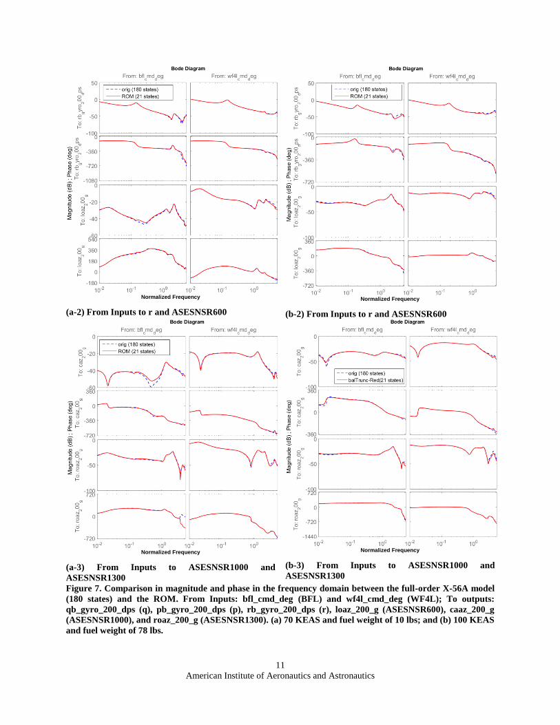
C ROM with Different Flight Parameters

A desired feature that will saliently enhance the utility of MOR for aircraft ASE analysis and controller synthesis

is its robustness and consistence of model configuration parameters regardless of the flight conditions. A thorough

study to investigate the effect of varying flight parameters (KEAS and fuel weights) on MOR performance was also

carried out. In the MOR analysis below, models with different flight parameters (KEAS = 70 or fuel weight of 78

lbs) from the benchmark case (100 KEAS and fuel weight of 10 lbs) were interrogated. Note that all the modeling

configuration parameters (number of states/dimensions to keep or truncate) at each step remained the same as the

case study in Section A above. Figure 7 illustrate the overall comparison of the magnitude and phase in the

frequency domain between the full-order X-56A model and the ROM with 21 states for the non-benchmark cases. It

shows that the ROMs at the new flight conditions are still able to accurately capture the dynamics in all input-output

channels in the entire frequency range of interest for control design. The minor deviation of ROM from the full-

order model only occurs at the middle-to-high frequency regime. The excellent ROM performance at various flight

conditions substantiates pronounced robustness and utility of our MOR methods.


(a-1) From Inputs to q and p


(b-1) From Inputs to q and p


11


(a-2) From Inputs to r and ASESNSR600


(b-2) From Inputs to r and ASESNSR600


(a-3) From Inputs to ASESNSR1000 and

ASESNSR1300


(b-3) From Inputs to ASESNSR1000 and

ASESNSR1300

Figure 7. Comparison in magnitude and phase in the frequency domain between the full-order X-56A model

(180 states) and the ROM. From Inputs: bfl_cmd_deg (BFL) and wf4l_cmd_deg (WF4L); To outputs:

qb_gyro_200_dps (q), pb_gyro_200_dps (p), rb_gyro_200_dps (r), loaz_200_g (ASESNSR600), caaz_200_g

(ASESNSR1000), and roaz_200_g (ASESNSR1300). (a) 70 KEAS and fuel weight of 10 lbs; and (b) 100 KEAS

and fuel weight of 78 lbs.


12

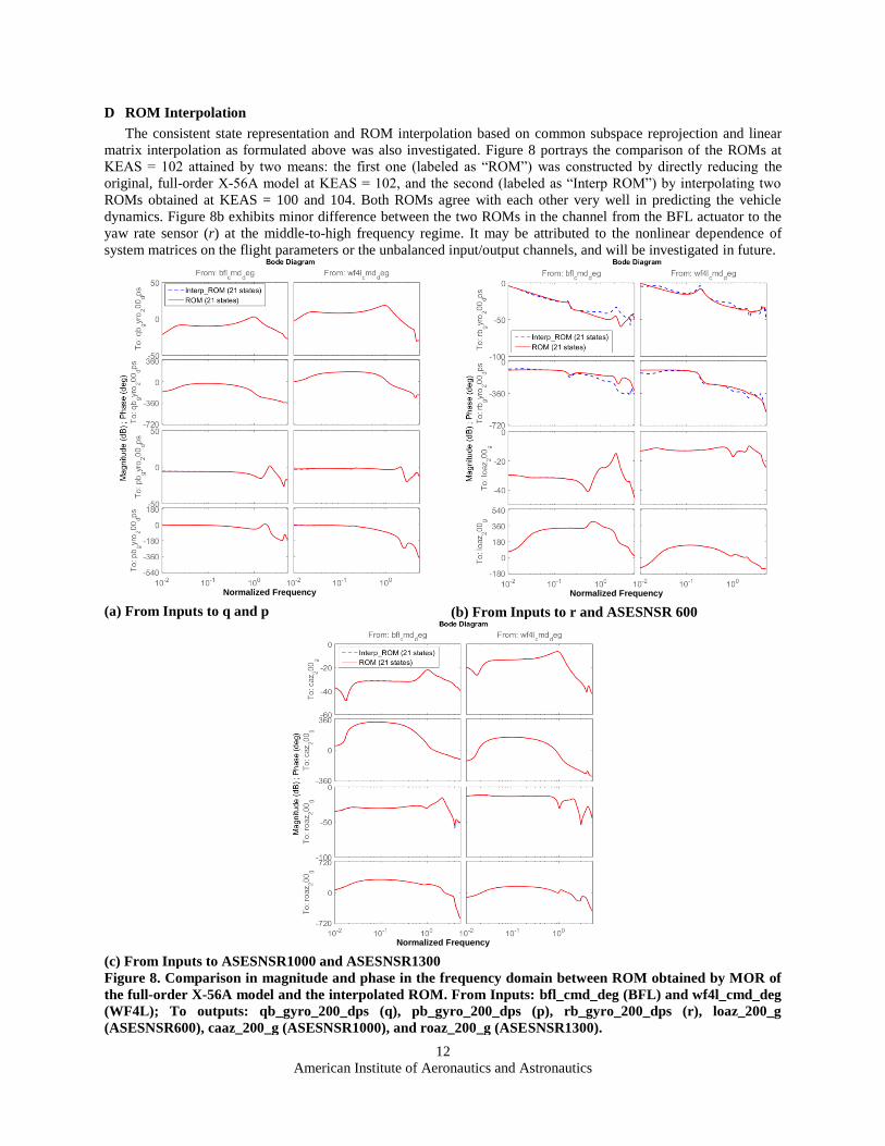
D ROM Interpolation

The consistent state representation and ROM interpolation based on common subspace reprojection and linear

matrix interpolation as formulated above was also investigated. Figure 8 portrays the comparison of the ROMs at

KEAS = 102 attained by two means: the first one (labeled as “ROM”) was constructed by directly reducing the

original, full-order X-56A model at KEAS = 102, and the second (labeled as “Interp ROM”) by interpolating two

ROMs obtained at KEAS = 100 and 104. Both ROMs agree with each other very well in predicting the vehicle

dynamics. Figure 8b exhibits minor difference between the two ROMs in the channel from the BFL actuator to the

yaw rate sensor (r) at the middle-to-high frequency regime. It may be attributed to the nonlinear dependence of

system matrices on the flight parameters or the unbalanced input/output channels, and will be investigated in future.


(a) From Inputs to q and p


(b) From Inputs to r and ASESNSR 600


(c) From Inputs to ASESNSR1000 and ASESNSR1300

Figure 8. Comparison in magnitude and phase in the frequency domain between ROM obtained by MOR of

the full-order X-56A model and the interpolated ROM. From Inputs: bfl_cmd_deg (BFL) and wf4l_cmd_deg

(WF4L); To outputs: qb_gyro_200_dps (q), pb_gyro_200_dps (p), rb_gyro_200_dps (r), loaz_200_g

(ASESNSR600), caaz_200_g (ASESNSR1000), and roaz_200_g (ASESNSR1300).


13

VI. Conclusion

This paper presented a holistic model order reduction (MOR) framework for constructing high-quality linear

parameter-varying aeroservoelastic reduced order models (ASE-ROMs) of flexible aircraft. Key MOR modules of

sequential model reduction, consistent model representation, and model interpolation have been established to

streamline the workflow. A suite of proven model reduction techniques, including truncation and residualization,

modal reduction, and balanced realization and truncation have been developed to determine optimal ROMs at grid

points across the flight envelope. A novel method combing singular value decomposition and common subspace

projection has been developed to unify the state representation for the ROMs obtained from non-orthonormal

transformation-based MOR. Parameter-weighted matrix interpolation has been carried out to construct a globally

functional LPV ASE ROM. The developed MOR technology has been applied to the X-56A MUTT vehicle with

flexible wing to examine its capability of generating reliable ROMs for control design. Our studies demonstrate that

the X-56A ROM was able to accurately describe vehicles dynamics and input/output response at various flight

conditions in the practically important frequency regime while the number of states in ROM was reduced by 10X.

The technology enables robust ASE controller synthesis for aircraft and novel vehicle design for flutter suppression

and gust load alleviation

Acknowledgments

This research is sponsored by NASA under contract NNX14CD04P.

References

1. Pak, C. and S. Lung, Flutter Analysis of Aerostructures Test Wing with Test Validated Structural Dynamic

Model. Journal of aircraft, 2011. 48(4): p. 1263-1272.

2. Sheta, E.F., et al., Computational and experimental investigation of limit cycle oscillations of nonlinear

aeroelastic systems. Journal of Aircraft, 2002. 39(1): p. 133-141.

3. Silva, W., et al. Development of Aeroservoelastic Analytical Models and Gust Load Alleviation Control Laws

of a SensorCraft Wind- Tunnel Model Using Measured Data. in 47th AIAA/ASME/ASCE/AHS/ASC Structures,

Structural Dynamics, and Materials Conference. 2006.

4. Hjartarson, A., P.J. Seiler, and G.J. Balas. Lpv aeroservoelastic control using the lpvtools toolbox. in AIAA

Atmospheric Flight Mechanics (AFM) Conference. 2013.

5. Theis, J., et al. Modal Matching for LPV Model Reduction of Aeroservoelastic Vehicles. in AIAA Atmospheric

Flight Mechanics Conference. 2015. Kissimmee, Florida.

6. Poussot-Vassal, C. and C. Roos. Flexible aircraft reduced-order LPV model generation from a set of large-

scale LTI models. in American Control Conference (ACC), 2011. 2011. IEEE.

7. Moreno, C.P., P.J. Seiler, and G.J. Balas, Model Reduction for Aeroservoelastic Systems. Journal of Aircraft,

2014. 51(1): p. 280-290.

8. Panzer, H., et al., Parametric model order reduction by matrix interpolation. at-Automatisierungstechnik

Methoden und Anwendungen der Steuerungs-, Regelungs-und Informationstechnik, 2010. 58(8): p. 475-484.

9. http://www.zonatech.com/ZAERO.htm.

10. http://www.mscsoftware.com/product/msc-nastran.

11. Adegas, F.D., et al. Reduced-order LPV model of flexible wind turbines from high fidelity aeroelastic codes.

in Control Applications (CCA), 2013 IEEE International Conference on. 2013. IEEE.

12. Pak, C.-g. and S. Truong. Creating a Test Validated Structural Dynamic Finite Element Model of the X-56A

Aircraft. in 5TH AIAA/ISSMO MULTIDISCIPLINARY ANALYSIS AND OPTIMIZATION CONFERENCE.

2014.

13. Hjartarson, A., P.J. Seiler, and G.J. Balas. Lpv aeroservoelastic control using the lpvtools toolbox. in AIAA

Atmospheric Flight Mechanics (AFM) Conference. 2013.

http://www.zonatech.com/ZAERO.htm

http://www.mscsoftware.com/product/msc-nastran

model order reduction of aeroservoelastic model of ... institute of aeronautics and astronautics 1...

Documents