1

Model-based Software Development

Application Model in SCADE (data flow + SSM)

Worst-Case Execution Time Analysis Stack Usage Analysis

System-level Schedulability Analysis

Generator

Compiler void Task (void) { variable++; function(); next++: if (next) do this; terminate() }

C-Code Binary Code Runtime Error Analysis

System Model (tasks, interrupts, buses, …)

SymTA/S

Astrée aiT

StackAnalyzer

SCADE Suite

2

The Task of a Compiler

Task of a compiler for a high-level programming language (C, C++, Java, ...) is

§  to transform an input program written in the high-level language §  into a semantically equivalent sequence of machine instructions of the

target processor §  that should have some desired properties:

§  being as short as possible, or §  being as fast as possible, or §  using as little energy as possible.

3

Why care?

ü  6 times faster! ü  Processor performance

depends on quality of code generation.

ü  Good code generation is a challenge.

C code (FIR Filter): int i,j,sum; for (i=0;i<N-M;i++) { sum=0; for (j=0;j<M;j++) { sum+=array1[i+j]*coeff[j]; } output[i]=sum>>15; }

Compiler-generated code (gcc): .L21: add %d15,%d3,%d1 addsc.a %a15,%a4,%d15,1 addsc.a %a2,%a5,%d1,1 mov %d4,49 ld.h %d0,[%a15]0 ld.h %d15,[%a2]0 madd %d2,%d2,%d0,%d15 add %d1,%d1,1 jge %d4,%d1,.L21

Hand-written code (inner loop): _8: ld16.w d5, [a2+] ld16.w d4, [a3+] madd.h e8,e8,d5,d4ul,#0 loop a7,_8

4

Middle End

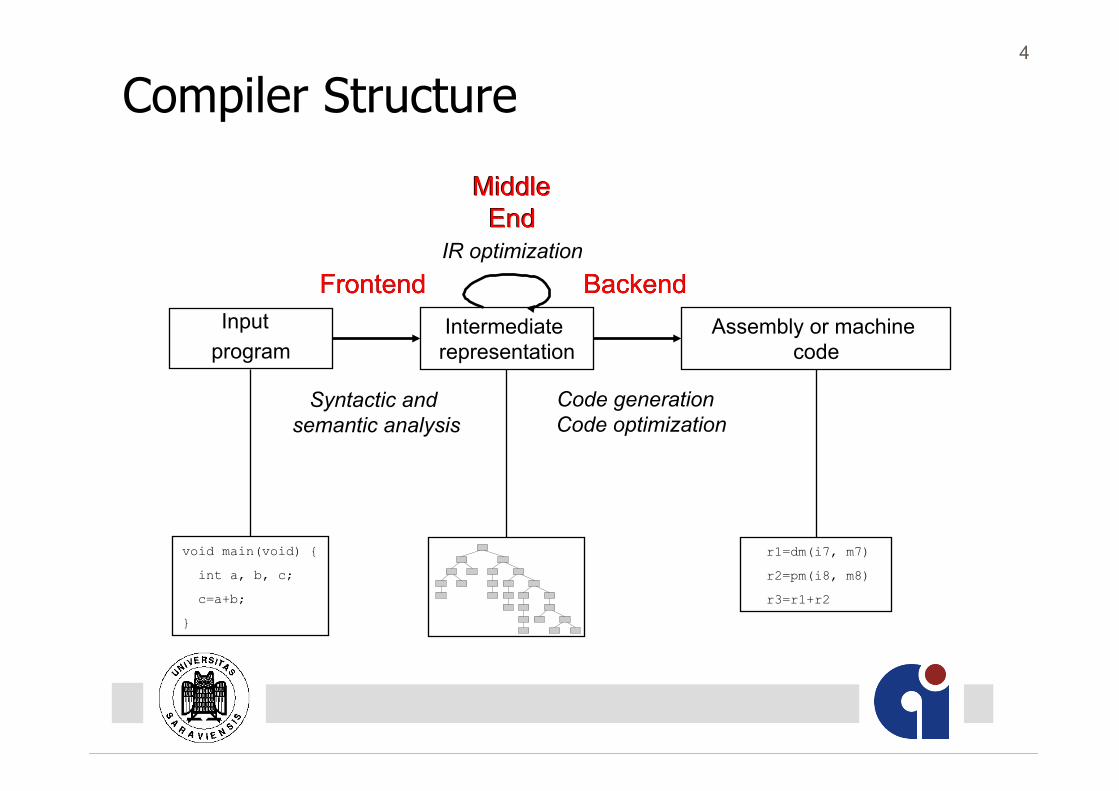
Compiler Structure

Input program

Intermediate representation

Assembly or machine code

void main(void) {

int a, b, c;

c=a+b;

}

r1=dm(i7, m7)

r2=pm(i8, m8)

r3=r1+r2

Frontend Backend Frontend

Syntactic and semantic analysis

Backend

Code generation Code optimization

Middle End

IR optimization

5

Detailed Compiler Structure

Source (Text)

Decorated Syntax Tree

High-Level Intermediate Representation

Lexical Analysis Syntactical Analysis Semantical Analysis

High-Level Optimizations

Low-Level Optimization and Code Generation

Machine Program

Low-Level Intermediate Representation

Middle- End

Back- End

13

r1=load adr(a)

r1=add r1, r2

r2=load adr(b)

store adr(c), r1

r1=load adr(a) || r2=load adr(b)

store adr(c), r1

r1=add r1, r2

c=a+b; load adr(a)

add

load adr(b)

store adr(c)

Code selection

Instruction scheduling

Register allocation

b c

a a

c b

Backend: Main Phases

14

Main Tasks of Code Generation (1) §  Code selection: Map the intermediate representation to a semantically

equivalent sequence of machine operations that is as efficient as possible.

§  Register allocation: Map the values of the intermediate representation to physical registers in order to minimize the number of memory references during program execution. §  Register allocation proper: Decide which variables and expressions of the

IR are mapped to registers and which ones are kept in memory. §  Register assignment: Determine the physical registers that are used to

store the values that have been previously selected to reside in registers.

15

Main Tasks of Code Generation (2) §  Instruction scheduling:

Reorder the produced operation stream in order to minimize pipeline stalls and exploit the available instruction-level parallelism.

§  Resource allocation / functional unit binding: Bind operations to machine resources, e.g. functional units or buses.

17

The Code Generation Problem §  Optimal code selection: NP-complete §  Optimal register allocation: NP-complete §  Optimal instruction scheduling: NP-complete §  All of them are interdependent, i.e. decisions made in one phase

may impose restrictions to the other. §  Usually they are addressed

§  by heuristic methods §  in separate phases.

§  Thus: often suboptimal combination of suboptimal partial results.

18

The Phase Ordering Problem

d1=s1*s1;

d2=s1+s2;

R3=R1*R1

store R3

R3=R1+R2

store R3

R3=r1*r1, R4=R1+R2

store R3

store R4

Optimize number of used registers

Optimize code speed and size

19

Impact of Code Selection struct { unsigned b1:1; unsigned b2:1; unsigned b3:1; } s; s.b3 = s.b1 && s.b2;

ld.bu d5, [sp]48 extr.u d5, d5, #0, #1 ne d5, d5, #0 mov16 d4, d5 jeq d4, #0, _9 ld.bu d4, [sp]48 extr.u d4, d4, #1, #1 ne d4, d4, #0 _9: ld.b d3, [sp]48 insert d3, d3, d4, #2, #1 st.b [sp]48, d3 9 cycles, 42 bytes

ld.bu d5, [sp]48 and.t d3, d5, #0, d5, #1 insert d5, d5, d3, #2, #1 st.b [sp]48, d5 3 cycles, 16 bytes

28

Intermediate Representations

§  Call Graph §  Control Flow Graph §  Basic Block Graph §  Data Dependence Graph

29

High-Level and Low-Level IRs §  High-level intermediate representation: close to source level.

Typically centered around source language constructs. Constructs: implicit memory addressing, expression trees, for- while-, switch-statements, etc.

§  Low-level intermediate representation: close to machine level. Typically centered around basic entities that specify properties of machine operations.

§  Most program representations can be defined at high-level and at low-level.

31

Call Graph §  There is a node for the main procedure – being the entry node

of the program – and a node for each procedure declared in the program.

§  The nodes are marked with the procedure names.

§  There is an edge between the node for a procedure p to the node of procedure q, if there is a call to q inside of p.

32

[y := x]1;

[z := 1]2;

while [y>1]3

do { [z := z*y]4;

[y := y-1]5

};

[y := 0]6

Control Flow Graph

[z := z*y]4

[y := 0]6 [y>1]3

[y := x]1

[z := 1]2

[y := y-1]5

33

Control Flow Graph §  The control flow graph of a procedure is a directed, node and edge

labeled graph GC=(NC,EC,nA,nΩ). §  For each instruction i of the procedure there is a node ni labeled i. §  An edge (n,m,λ) with edge label λ ∈ {T,F,ε} denotes control flow of a

procedure. §  Subgraphs for composed statements are shown on the next slide. §  Edges belonging to unconditional branches lead from the node of the

branch to the branch destination. §  node nA is the uniquely determined entry point of the procedure;

it belongs to the first instruction to be executed. §  nΩ is the end node of any path through the control flow graph.

§  Nodes with more than one predecessor are called joins and nodes with

more than one successor are called forks.

34

cfg (while B do S od) =

cfg (S)

B F

T

cfg (if B then S else S fi) =1 2

BT F

cfg (S )1 cfg (S )2

cfg (S )1

cfg (S )2

cfg (S ;S ) =1 2

Control Flow Graph – Composed Statements

35

Basic Block Graph §  A basic block in a control flow graph is a path of maximal length which

has no joins except at the beginning and no forks except possibly at the end.

§  The basic block graph GB=(NB,EB,bA,bΩ) of a control flow graph GC=(NC,EC,nA,nΩ) is formed from GC by combining each basic block into a node.

§  Edges of GC leading into the first node of a basic block lead to the node of that basic block in GB.

§  Edges of GC leaving the last node of a basic block lead out of the node of that basic block in GB.

§  The node bA denotes the uniquely determined entry block of the procedure;

§  bΩ denotes the exit block that is reached at the end of any path through the procedure.

46

Types of Microprocessors §  Complex Instruction Set Computer (CISC)

§  large number of complex addressing modes §  many versions of instructions for different operands §  different execution times for instructions §  few processor registers §  microprogrammed control logic

§  Reduced Instruction Set Computer (RISC)

§  one instruction per clock cycle §  memory accesses by dedicated load/store instructions §  few addressing modes §  hard-wired control logic

47

Example Instruction (IA-32)

Execution time: •  1 cycle: ADD EAX, EBX •  2 cycles: ADD EAX, memvar32 •  3 cycles: ADD memvar32, EAX •  4 cycles: ADD memvar16, AX

Instruction Width: between 1 byte (NOP) and 16 bytes

48

Types of Microprocessors §  Superscalar Processors

§  subclass of RISCs or CISCs §  multiple instruction pipelines for overlapping execution of

instructions §  parallelism not necessarily exposed to the compiler

§  Very Long Instruction Word (VLIW) §  statically determined instruction-level parallelism (under compiler

control) §  instructions are composed of different machine operations whose

execution is started in parallel §  many parallel functional units §  large register sets

49

VLIW Architectures

operation 1 … operation 2 operation 0

instruction slot 0 instruction slot 1

50

Characteristics of Embedded Processors §  Multiply-accumulate units: multiplication and accumulation in a single

clock cycle (vector products, digital filters, correlation, fourier transforms, etc)

§  Multiple-access memory architectures for high bandwidth between processor and memory §  Goal: throughput of one operation per clock cycle. §  Required: several memory accesses per clock cycle. §  Separate data and program memory space: harvard architecture. §  Multiple memory banks §  Arithmetic operations in parallel to memory accesses. But often

irregular restrictions.

§  Specialized addressing modes, e.g. bit-reverse addressing or auto-modify addressing.

51

§  Predicated/guarded execution: instruction execution depends on the value of explicitly specified bit values or registers.

§  Hardware loops / zero overhead loops: no explicit loop counter increment/decrement, no loop condition check, no branch back to top of loop

§  Restricted interconnectivity between registers and functional units -> phase coupling problems.

§  Strongly encoded instruction formats: a throughput of one instruction per clock cycle requires one instruction to be fetched per cycle. Thus each instruction has to fit in one memory word => reduction of bit width of the instruction.

Characteristics of Embedded Processors

52

a=b+c*z[i+0] d=e+f*z[i+1] r=s+t*z[i+2] w=x+y*z[i+3]

b e s x

c f t y

z[i+0] z[i+1] z[i+2] z[i+3]

= +SIMD *SIMD

a d r w

⇒

op

Halfword 0 Halfword 1

Halfword0 Halfword1

Destination0 Destination1

§  SIMD instructions: §  Focus on multimedia applications §  SIMD: Single Instruction Multiple

Data §  SIMD-Instruction: instruction

operating concurrently on data that are packed in a single register or memory location.

Characteristics of Embedded Processors

53

§  Cost constraints, low power requirements and specialization:

Ø Irregularity

Ø Phase coupling problems during code generation

Ø Need for specialized algorithms

Characteristics of Embedded Processors

54

The Phase Coupling Problem §  Main subtasks of compiler backends:

§  code selection: mapping of IR statements to machine instructions of the target processor

§  register allocation: map variables and expressions to registers in order to minimize the number of memory references during program execution

§  register assignment: determine the physical register used to store a value that has been previously selected to reside in a register

§  instruction scheduling: reorder an instruction sequence in order to exploit instruction-level parallelism and minimize pipeline stalls

§  resource allocation: assign functional units and buses to operations

55

The Phase Coupling Problem §  Classical approaches: isolated solution by heuristic methods (list

scheduling, trace scheduling, graph coloring register allocation, etc).

⇒ Problem: interdependence of code generation phases. ⇒ Suboptimal combination of suboptimal partial results. ⇒ Inefficient code.

§  Solution in a perfect world: Address all problems simultaneously in a single phase. BUT: §  How to formulate this? §  Code selection, register allocation/register assignment and instruction

scheduling by themselves are NP-hard problems. §  This means that in general there is no chance to optimally solve even one

single of these tasks separately.

56

Code Selection and Register Allocation §  The goal of code selection is to determine the cheapest instruction

sequence for a subgraph of the IR. However, the code selector does not know what the real overall costs of the instruction sequence will be; it can use only estimations.

§  Register allocation usually is done after code selection so the code selector typically has to assume an infinite number of registers (virtual registers).

§  In consequence when estimating the cost of an instruction sequence the code selector will mostly assume register references.

§  Register allocation has to cope with a finite number of registers. If there are too few registers, spill code is generated.

§  However, the cost of this spill code has not been considered during code selection, so the chosen operation sequence may in fact be a bad choice since another one might have worked without spill code.