model-based heuristics for combinatorial optimization: · pdf fileinstitut fur angewandte...
TRANSCRIPT
Institut fur Angewandte Stochastik und Operations Research
Model-based heuristics for combinatorialoptimization: a mathematical study of their
asymptotic behavior
PhD Thesis
January 4, 2015
Author:Zijun Wu
Supervisor:Prof. Dr. Michael Kolonko

Declaration
I hereby declare that except where specific reference is made to the work of others, thecontents of this dissertation are original and have not been submitted in whole or in partfor consideration for any other degree or qualification in this, or any other university.This dissertation is my own work and contains nothing which is the outcome of workdone in collaboration with others, except as specified in the text and Acknowledgement.
Signed:Date:
ii

Acknowledgement
First, I want to sincerely thank my supervisor Mr Prof. Dr. Michael Kolonko. He gaveme much support in my study and led me to such an interesting field. And I also wantto thank him for agreeing me to collect our co-work in this Thesis.
Then, I want to thank my colleagues Mr Dipl.-inf Stephan Mock, Mr M.Sc ZhixingYang, Mr Dipl.-Math. Fabian Kirchnoff, Miss Gesine Redecker and Miss BaerbelHeise-Kretzer, they gave me numerous help during my stay in Clausthal.
I also want to thank my wife. Without her understanding and support, I would nothave been able to concentrate on my study.
Special thank goes to the Chinese Government, they financially supported my studyfrom December 2010 to November 2014.
iii

Abstract
Due to the complexity of many important combinatorial optimization problems, heuris-tic search algorithms are of overwhelming importance for a practical solution of manyproblems in Operations Research like tour planing, vehicle routing, scheduling, pack-ing etc. Many traditional heuristic procedures are ‘solution-based’, e.g. tabu search,simulated annealing, genetic algorithms etc. Here, new solutions are produced troughmanipulating current solutions with a specified strategy like edge exchanging in tourplanning, crossover and mutation in genetic algorithms etc.
Recently, a different class of algorithms have gained attention which do not concentrateon solutions, but on the mechanism to produce them. The mechanism is typically adistribution on the space of solutions. It is often called a ‘model’ for the solution space,and new solutions are produced by sampling from it. Starting from a fixed initial model,these algorithms then iteratively evolve the present model by adapting it to some ‘best’solutions sampled from the present model and/or previous models. By the evolution,they expect to reach a model concentrating only on some optimal solutions. Examplesof these ‘model-based’ heuristic procedures include ant colony optimization algorithms,cross entropy algorithms and estimation of distribution algorithms.
This Thesis concentrates on these model-based heuristics i.e. model-based search. Wepropose a framework which covers the essential features of these algorithms in practice.The framework contains a new concept which can include probabilistic dependenciesinto the sampling. We study closely the resulting stochastic process of the framework.We state simple conditions which guarantee to reach an optimal solution in finitelymany iterations. For some standard test problems, we show conditions which imply a(low-degree) polynomial runtime with a probability converging to 1 as the problem sizeapproaches infinity.
We also investigate the asymptotic properties of the samples and models. We showthat the sampling may get frozen at a fixed solution after finitely many iterations, andthe models may converge to one-point measure. This theoretically proves the stagnationbehavior observed in the literature. In particular, we propose conditions which makethe models converge to a limit concentrating only on optimal solutions.
We complement the theoretical analysis with a computational study on the famoustraveling salesman problem. The experimental results clearly demonstrate our theoreti-cal findings, and show some useful hints for a practice use.
Keywords:combinatorial optimization; heuristics; ant colony optimization; cross entropy;estimation of distribution algorithms; distribution learning; convergence; runtimeanalysis; genetic drift; unsupervised learning; stochastic process.
iv

Acronyms
MMAS MAX -MIN ant system. 31
ACO ant colony optimization. 23
ACS ant colony system. 30
AP assignment problem. 9
AS ant system. 26
CE cross entropy algorithm. 16
cGA compact genetic algorithm. 43
CO combinatorial optimization. 6
COP combinatorial optimization problem. 8
EDA estimation of distribution algorithms. 37
FIFO first in first out. 59
GTMU globally truncate memory update. 59
ID identity selection. 60
KP knapsack problem. 9
LTMU locally truncate memory update. 59
MaxCut maximal cut problem. 9
MBS model-based search. 11
MID memory identical selection. 60
MRS memory random selection. 60
NM non memory. 59
v

Ph. D Thesis Technical University of Clausthal
PBAS population-based ant system. 31, 59
PBIL population-based incremental learning. 41
RES rare event simulation. 149
RS random selection. 60
SBS solution-based search. 11
TDWL time dependent weighted learning. 61
TS truncate selection. 60
TSP traveling salesman problem. 8
UL uniform learning. 60
UMDA univariate marginal distribution algorithm. 40
WL weighted learning. 60, 61
WO worst out. 59
Acronyms vi

Contents
Declaration ii
Acknowledgement iii
Abstract iv
Acronyms v
List of Figures x
List of Tables xi
List of Symbols xii
1 Introduction 1
2 Background: combinatorial optimization and heuristic search 62.1 Combinatorial optimization: some elements . . . . . . . . . . . . . . . . . 62.2 Combinatorial optimization: examples . . . . . . . . . . . . . . . . . . . . 8
2.2.1 Traveling salesman problem . . . . . . . . . . . . . . . . . . . . . . 82.2.2 Assignment problem . . . . . . . . . . . . . . . . . . . . . . . . . . 82.2.3 Maximal cut problem . . . . . . . . . . . . . . . . . . . . . . . . . 92.2.4 Knapsack problem . . . . . . . . . . . . . . . . . . . . . . . . . . . 9
2.3 Heuristic search . . . . . . . . . . . . . . . . . . . . . . . . . . . . . . . . . 102.3.1 Search algorithms in combinatorial optimization . . . . . . . . . . 102.3.2 A classification to heuristic search: solution-based v.s. model-based 11
3 A short tutorial on model-based search algorithms used in practice 133.1 A common motivation . . . . . . . . . . . . . . . . . . . . . . . . . . . . . 143.2 Example I: cross entropy algorithm . . . . . . . . . . . . . . . . . . . . . . 16
3.2.1 Representation of feasible solutions . . . . . . . . . . . . . . . . . . 163.2.2 The specified model family for cross entropy algorithm . . . . . . . 173.2.3 The algorithm . . . . . . . . . . . . . . . . . . . . . . . . . . . . . 183.2.4 A brief introduction to CE variants . . . . . . . . . . . . . . . . . . 20
3.3 Example II: ant colony optimization . . . . . . . . . . . . . . . . . . . . . 233.3.1 The foraging behavior of ants . . . . . . . . . . . . . . . . . . . . . 233.3.2 Representation of solutions: walks on a construction graph . . . . 253.3.3 Ant System: the first ACO algorithm . . . . . . . . . . . . . . . . 26
vii
Ph. D Thesis Technical University of Clausthal
3.3.4 Ant colony system . . . . . . . . . . . . . . . . . . . . . . . . . . . 303.3.5 MAX -MIN ant system . . . . . . . . . . . . . . . . . . . . . . . 313.3.6 Population-based ant system . . . . . . . . . . . . . . . . . . . . . 31
3.4 Example III: estimation of distribution algorithms . . . . . . . . . . . . . 373.4.1 Feasible solutions and univariate models . . . . . . . . . . . . . . . 373.4.2 Simulating uniform crossover by a univariate marginal model . . . 383.4.3 Univariate marginal distribution algorithm . . . . . . . . . . . . . 403.4.4 Population based incremental learning . . . . . . . . . . . . . . . . 413.4.5 Compact genetic algorithm . . . . . . . . . . . . . . . . . . . . . . 43
4 A unified model-based search framework 454.1 A unified representation of feasible solutions . . . . . . . . . . . . . . . . . 46
4.1.1 Representing feasible solutions as strings . . . . . . . . . . . . . . . 464.1.2 Relation with other frequently used representations . . . . . . . . . 484.1.3 Introducing constraints under string encoding . . . . . . . . . . . . 48
4.2 A unified model family and feasibility construction . . . . . . . . . . . . . 504.2.1 A review to the model family Pce . . . . . . . . . . . . . . . . . . . 504.2.2 A unified sampling mechanism: feasible construction . . . . . . . . 514.2.3 Cover the sampling of ACO . . . . . . . . . . . . . . . . . . . . . . 534.2.4 Probabilistic dependencies in the sampling . . . . . . . . . . . . . 56
4.3 A unified model-based search framework . . . . . . . . . . . . . . . . . . . 574.3.1 The unified framework for model-based search . . . . . . . . . . . 574.3.2 A summary of commonly-used rules in practical model-based search
algorithms . . . . . . . . . . . . . . . . . . . . . . . . . . . . . . . . 594.3.3 Selection rules . . . . . . . . . . . . . . . . . . . . . . . . . . . . . 604.3.4 The learning rules . . . . . . . . . . . . . . . . . . . . . . . . . . . 604.3.5 Distribution update rules . . . . . . . . . . . . . . . . . . . . . . . 61
4.4 The underlying stochastic process . . . . . . . . . . . . . . . . . . . . . . . 634.4.1 Input parameters and strategy . . . . . . . . . . . . . . . . . . . . 634.4.2 The underlying stochastic process . . . . . . . . . . . . . . . . . . 63
5 Analysis of model-based search I: reachability and a crude runtime analysis 675.1 Definitions and assumptions . . . . . . . . . . . . . . . . . . . . . . . . . . 69
5.1.1 Definitions . . . . . . . . . . . . . . . . . . . . . . . . . . . . . . . 695.1.2 General assumptions . . . . . . . . . . . . . . . . . . . . . . . . . . 70
5.2 Some basic properties . . . . . . . . . . . . . . . . . . . . . . . . . . . . . 725.2.1 On basic recursion . . . . . . . . . . . . . . . . . . . . . . . . . . . 725.2.2 A surrogate probability of Q(·; y, i,Π) and its properties . . . . . . 75
5.3 On the reachability of optimal solutions . . . . . . . . . . . . . . . . . . . 815.3.1 Related work . . . . . . . . . . . . . . . . . . . . . . . . . . . . . . 815.3.2 A unified theorem for reachability of optimal solutions . . . . . . . 81
5.4 Some runtime analysis results . . . . . . . . . . . . . . . . . . . . . . . . . 865.4.1 Definitions of two test problems . . . . . . . . . . . . . . . . . . . . 865.4.2 Runtime results for unrestricted models . . . . . . . . . . . . . . . 86
Contents viii
Ph. D Thesis Technical University of Clausthal
5.4.3 Runtime results for restricted models . . . . . . . . . . . . . . . . . 91
6 Analysis of model-based search II: absorption of solutions and models 976.1 Definitions and some additional assumptions . . . . . . . . . . . . . . . . 98
6.1.1 Definitions . . . . . . . . . . . . . . . . . . . . . . . . . . . . . . . 986.1.2 Some additional assumptions . . . . . . . . . . . . . . . . . . . . . 98
6.2 Absorption of solutions in model-based search . . . . . . . . . . . . . . . . 1006.2.1 A universal absorption Theorem . . . . . . . . . . . . . . . . . . . 1006.2.2 A general method for time inhomogeneous Markov chain . . . . . . 1076.2.3 On the absorbing solution s<∞ . . . . . . . . . . . . . . . . . . . . 109
6.3 Absorption of models . . . . . . . . . . . . . . . . . . . . . . . . . . . . . . 114
7 An experimental study 1217.1 Random tour generation and learning . . . . . . . . . . . . . . . . . . . . 122
7.1.1 Random solution generation . . . . . . . . . . . . . . . . . . . . . . 1227.1.2 Learning the empirical distribution Wt . . . . . . . . . . . . . . . 123
7.2 Experimental study . . . . . . . . . . . . . . . . . . . . . . . . . . . . . . . 1247.2.1 The test instance . . . . . . . . . . . . . . . . . . . . . . . . . . . . 1247.2.2 Experimental setting . . . . . . . . . . . . . . . . . . . . . . . . . . 1257.2.3 Results under non-greedy feasibility construction . . . . . . . . . . 1257.2.4 Under greedy feasibility construction . . . . . . . . . . . . . . . . . 134
8 Summary and future work 139
Appendix 141A.1 Some definitions in graph theory . . . . . . . . . . . . . . . . . . . . . . . 141A.2 Shannon Entropy, K-L divergence and importance sampling . . . . . . . . 143A.3 Linear programming and integer programming . . . . . . . . . . . . . . . . 144A.4 Elements about probability theory and stochastic process . . . . . . . . . 145A.5 Useful notations in runtime analysis . . . . . . . . . . . . . . . . . . . . . 148A.6 Application of cross entropy in rare event simulation . . . . . . . . . . . . 149A.7 Genetic algorithms and Local search . . . . . . . . . . . . . . . . . . . . . 155
Bibliography 159
Index 166
Contents ix

List of Figures
3.1 A visualization of P(A) for |A| = 3 . . . . . . . . . . . . . . . . . . . . . . 183.2 Cross entropy algorithm in combinatorial optimization . . . . . . . . . . . 223.3 A demo of ants foraging behavior . . . . . . . . . . . . . . . . . . . . . . . 233.4 Examples of graphs . . . . . . . . . . . . . . . . . . . . . . . . . . . . . . . 253.5 Ant system . . . . . . . . . . . . . . . . . . . . . . . . . . . . . . . . . . . 333.6 Ant colony system algorithm . . . . . . . . . . . . . . . . . . . . . . . . . 343.7 MAX -MIN ant system . . . . . . . . . . . . . . . . . . . . . . . . . . . 353.8 Population based ant system . . . . . . . . . . . . . . . . . . . . . . . . . 363.9 Univariate marginal distribution algorithm . . . . . . . . . . . . . . . . . . 423.10 Population-based incremental learning . . . . . . . . . . . . . . . . . . . . 433.11 Compact genetic algorithm . . . . . . . . . . . . . . . . . . . . . . . . . . 44
4.1 Random solution generation by feasibility construction . . . . . . . . . . . 524.2 A unified model-based search framework for combinatorial optimization . 584.3 Underlying process . . . . . . . . . . . . . . . . . . . . . . . . . . . . . . . 64
7.1 A TSP test instance . . . . . . . . . . . . . . . . . . . . . . . . . . . . . . 1257.2 Plots of the iteration best, iteration worst and best so far costs . . . . . . 1287.3 Observation of absorption of solutions and models . . . . . . . . . . . . . 1307.4 Observation of absorption of solutions and models (cont.) . . . . . . . . . 1317.5 Relation of ρ and best found solution . . . . . . . . . . . . . . . . . . . . . 1327.6 ρ and absorption . . . . . . . . . . . . . . . . . . . . . . . . . . . . . . . . 1337.7 ρ and best found solution for greedy case . . . . . . . . . . . . . . . . . . 1357.8 ρ and absorption for greedy case . . . . . . . . . . . . . . . . . . . . . . . 1367.9 Comparison . . . . . . . . . . . . . . . . . . . . . . . . . . . . . . . . . . . 137
1 Cross entropy algorithm for rare event simulation . . . . . . . . . . . . . . 1542 Genetic algorithm . . . . . . . . . . . . . . . . . . . . . . . . . . . . . . . 1563 Simulated annealing . . . . . . . . . . . . . . . . . . . . . . . . . . . . . . 157
x

List of Tables
4.1 The four rules for some practical MBS algorithms . . . . . . . . . . . . . . 62
5.1 The levels w∗t for the empirical distributions . . . . . . . . . . . . . . . . 89
7.1 Point sets for test instance . . . . . . . . . . . . . . . . . . . . . . . . . . . 1267.2 Implementation results for non greedy case . . . . . . . . . . . . . . . . . 1277.3 Implementation results for greedy case . . . . . . . . . . . . . . . . . . . . 134
xi

List of Symbols
Ci(·; ·) the priori feasibility distribution for position i+ 1. 51
Ci(y) the support of feasibility distribution Ci(y; ·). 51
L the encoded solution length in a string encoding. 16
Q(a; y, i+ 1,Π) the selection probability for alphabet a at position i+1 when the leadingpartial solution is y ∈ Ri in a feasibility construction. 52
Q((s1, . . . , sL); Π
)the selection probability for a solution (s1, . . . , sL) in a feasibility
construction. 52
Ri the collection of partial solutions with length i. 51
S∗ set of optimal solutions. 6
S feasible solutions. 6
1A indicator function of a set A. 9
A the finite alphabet for an instance in string encoding. 16
L learning rale. 63
Mt the memory for iteration t. 57
M memory update rule. 63
N natural numbers. 17
N bt the selected subsample from Mt ∪Xt. 57
the empty string. 47
Π(a; i) the probability of alphabet a occurring at position i under distribution Π. 17
Πt the model in iteration t. 15
R+ set of positive real numbers. 17
R set of real numbers. 6
S selection rule. 63
xii

Ph. D Thesis Technical University of Clausthal
Wt the empirical model for iteration t learned from N bt . 18
Xt the random sample in iteration t. 15
∈ the belonging relation. 8
f objective function, cost function. 6
List of Symbols xiii
1 Introduction
Combinatorial optimization [KV02] is a very important topic in applied mathematicsand theoretical computer science. It can be simply stated as finding out an object froma finite collection of candidates which minimizes (or maximizes) an associated objectivefunction. A well-known problem involving combinatorial optimization is the travelingsalesman problem (TSP), which concerns finding a shortest tour that starts in a city,traverses each other city exactly once, and finally returns to the start city. Actually,combinatorial optimization can be seen almost everywhere in reality. In logistics, wemay need to determine routes with a minimal total delivering cost for a fleet of vehicleswhich are employed to deliver goods from a central depot to consumers who ordered thegoods. In a water supply system, we may need to place several valves at pipes’ extremessuch that when a pipe breaks, it is possible to isolate it with minimal damage to the restof the network. In a factory, we may need to arrange some jobs on some machines suchthat the resulting makespan becomes minimal. In a harbor, we may need to determinea minimal number of ships for loading certain goods which are of different volumes andshapes.
In combinatorial optimization, we often call the collection of candidates a feasible set,an object belonging to the collection a feasible solution, and a feasible solution min-imizing (or maximizing) the associated objective function an optimal solution. Here,the objective is to find an optimal solution from the finite feasible set. In mathe-matical optimization, combinatorial optimization is usually categorized as a subtopicof discrete optimization. It is closely related to operations research, algorithm theoryand computational complexity theory. It has important applications in other fields liketransportation, machine learning, artificial intelligence, software engineering, job shopmanagement, information and communication techniques etc.
Due to the discrete nature, generally we can not get an analytic solution for a com-binatorial optimization problem. Thanks to the dramatically increased computationalcapacity in recent years, we now can exactly solve many combinatorial optimizationproblems under a moderate size by running an exact search [Woe03] on a computer,e.g. we may enumerate all feasible solutions. However, as the problem size increases,the complexity of the problems may increase exponentially. When the problem size isrelatively large, we may not get an exact optimal solution in an acceptable run time.To quickly obtain a practical solution in the case of a large problem size, we have toemploy some non-exact search procedures. Generally, these procedures can be collectedin two classes: approximation algorithms [WS11] and heuristics [Nic07]. Approximationalgorithms are those which are designed according to some particular features of theunderlying problem, and guarantee to find a high-quality approximation for the opti-mal solutions. Typically, they can guarantee that the approximation is optimal up to
1

Ph. D Thesis Technical University of Clausthal
a small constant factor, say 5%. However, they may depend heavily on the structure ofthe underlying problem, therefore can not be used for a general-purpose.
Heuristics do not guarantee on solutions’ qualities. However, many applications havedemonstrated that they can reach high-quality solutions in most cases. They are oftenequipped with some ‘intelligent’ or ‘self-adaptive’ mechanisms. These mechanisms areused to guide the underlying search in the feasible set. But, these mechanisms are gen-erally designed without involving much prior knowledge about the underlying problem.This makes heuristics rather portable in practice. So, heuristics can be seen as general-purpose tools for optimization. As a general-purpose tool, heuristics can be used inmany other fields, e.g. bioinformatics, machine learning, artificial intelligence.
Heuristics can be collected in two subclasses: solution-based heuristics (search) andmodel-based heuristics (search), see [ZBMD04]. Solution-based search concentrates onsolutions. They iteratively evolve solutions. New solutions are produced by manipulatingpresent solutions in a way that we can expect a better solution in the next round. Manytraditional heuristics are solution-based. Examples are these nature-like algorithms astabu search [GL99], simulated annealing [BT93], genetic algorithms [Mic96] etc. Here,new solutions are produced by changing and/or exchanging components on present so-lutions such that new solutions will ‘inherit’ good properties of present solutions. Forexample, when we apply a genetic algorithm to a TSP, new tours (solutions) are producedby performing crossover (exchanging edges on two selected parent tours) and mutation(randomly changing one edge on a child) on the present tours. More recent examplesof solution-based search are some swarm intelligence algorithms, including artificial beecolony [KGOK12], particle swarm optimization [KE95] and electromagnetism-like algo-rithm [BF03] etc. They aim to simulate the ‘collective’ behavior in a school of practicalcreatures. They iteratively evolve a swarm of solutions. The evolution of each individual(solution) in the swarm may refer to both its own history and the histories of its com-panions. For example, in a particle swarm optimization, an individual is evolved withreference to both its own best experience and the global best experience accumulatedby the whole swarm.
Model-based search does not concentrate on solutions, but on the mechanism to pro-duce solutions. This mechanism often explains the structure of the underlying problemto some extent. It is therefore called a ‘model’ of the problem or its solutions. Typically,it is a probabilistic distribution on the feasible set. Here, new solutions are produced bysampling from a present model. Model-based search iteratively evolves models instead ofsolutions. By evolution, they aim to reach a model which can produce optimal solutionsonly or with an overwhelming probability. Examples of model-based search are crossentropy algorithms [RK04], ant colony optimization algorithms [DS04], and estimationof distribution algorithms [HP11]. Starting from an arbitrarily fixed initial model Π0,model-based search then iteratively evolve models as, for t = 0, 1, 2, . . . ,
Sampling: generate a random sample Xt of a specified size N ∈ N by the present modelΠt;
Learning: learn an empirical model Wt from a subsample N bt consisting of some selected
‘best’ solutions which are seen in present sample Xt and/or in history;
2

Ph. D Thesis Technical University of Clausthal
Update: set the next model Πt+1 = (1 − ρt+1)Πt + ρt+1Wt, where ρt+1 ∈ (0, 1] is alearning rate fixed in advance.
In combinatorial optimization, the feasible set is finite. A model (or a distribution)can be therefore described by a vector. So, the next model Πt+1 is actually a convexcombination of present model Πt and the learned empirical model Wt, where the learningrate ρt+1 reflects the relative importance of Wt in the combination. The subsample N b
t
typically consists of some best solutions seen in Xt and history, for example, it mayconsist only of best solution found so far or of some elite solutions in present sampleXt. By learning from N b
t , the empirical model Wt may contain information aboutgood solutions. By the combination, the next model Πt+1 is therefore biased towardsgood solutions. Thereby, we may expect that in the next sampling, more good solutionswill be produced. By iteratively evolving through the three steps, we hope that theresulting models process
(Πt
)t=0,1,2,...
can converge to a limit Π∞ concentrating onoptimal solutions i.e. the probability for producing optimal solutions by Π∞ is 1. So,in model-based search, we actually ‘optimize’ the mechanism for producing (optimal)solutions.
Model-based search may also apply to other fields. Typically, they can apply to rareevent simulation which usually concerns calculating the probability of a rare event ina complex system, see [RT+09] or A. 6 in Appendix. Due to the rarity of the event,the classic monte-carlo method may fail to give an effective approximation to that prob-ability. Here, a well-known approach is to employ importance sampling under a bestchange of measure selected from a specified family of candidate measures (distributionor density). Since model-based search evolve models (distributions), they can be appliedeasily to select the best change of measure. A successful example is the cross entropyalgorithm for rare event simulation, see [Rub97] and [Rub99].
Model-based search are closely related to other fields involving estimation of distribu-tion or density. A typical example is the so-called unsupervised learning in the field ofmachine learning [Alp10]. In unsupervised learning, we want to detect the regularitiesconcealed in the input data. Typically, we may build a multivariate distribution (or adensity) which fits the input observations best. By this distribution, we can determinethe mutual dependencies of different variables. This may coincide with the ‘Learning’step in model-based search. They can therefore share the learning method. A methodused in the ‘Learning’ step may also apply to unsupervised learning, and vice versa. Forexample, the Bayesian network is used in both Bayesian optimization algorithm [Pel05]and the unsupervised learning.
This Thesis concentrates on model-based search. We will inspect their long-termbehavior in combinatorial optimization. To do this, we will build a framework whichcan cover the essential features of these model-based search algorithms used in practice.The framework will result in a mixed Markov process, i.e. some marginal processesare discrete and other marginals are continuous. We will do a thorough mathematicalanalysis of this mixed process. Special emphasis will be given to the marginal processesformed by samples Xt and models Πt. Due to the non-homogeneity and complexity ofthe mixed process, we will not go along with the classical analysis for Markov chain. Our
3

Ph. D Thesis Technical University of Clausthal
analysis will involve only the memory-less property of the Markov chain. However, somebasic knowledge about probability theory is required. Readers who are not familiar withprobability theory can see A. 4 in the Appendix as a reference.
We will launch the analysis by stating simple conditions for guaranteeing to reach anoptimal solution. These conditions should be of great interests in practice. In [Gut00]and [Gut03], W. J. Gutjahr showed that for a particular ant colony optimization al-gorithm, we can increase the occurring probability of optimal solutions by decreasingthe evaporation rate (learning rate) or increasing the sample size N . In [CJK07], A.Costa et al inspected some important asymptotic properties of a generalized cross en-tropy algorithm for unconstrained combinatorial optimization problems. They showedconditions guaranteeing to reach an optimal solution. In our former work [WK14b], mysupervisor and I inspected a more general cross entropy optimization algorithm whichalso covers the essential features of some ant colony optimization algorithms. In thatwork, we did not impose any restriction on the underlying problem. Still, we are ableto show that the conditions proposed in [CJK07] hold in the more general algorithm. InChapter 5, we will continue the study of our former work. We show that the findings in[Gut00], [Gut03], [CJK07] and [WK14b] also hold in our more general framework, seeTheorem 5.7. Therefore, they may apply to all algorithms covered by the framework.In particular, we find that for the popular case ρt ≡ ρ > 0 used in practice, optimalsolutions may not occur.
In recent years, the runtime analysis for heuristics has become a very popular field, seee.g. [NW06], [NW09], [DNSW07], [DJ07], [Gut07], [Gut08], [CTCY10] and [WK14b]. Inruntime analysis, we want to find conditions which make an algorithm reach an optimalsolution efficiently with a high probability. Here, the runtime is a rudimentary copy ofthe computational complexity in theoretical computer science. It is generally defined asthe total number of solutions evaluated before reaching an optimal solution. In [NW06],[NW09], [DNSW07], [DJ07], [Gut07], [Gut08], researchers considered runtime for antcolony optimization algorithms with restricted models on some simple test problems likeOneMax and LeadingOne. They found that the runtime is closely related to the learningrate, and we may reach an optimal solution efficiently by adapting a constant learningrate to the problem size if we use restricted models. In [CTCY10], Chen et al initiateda different study for the case of non-restricted models. They inspected the runtime fora univariate marginal distribution algorithm (a particular cross entropy algorithm withρt ≡ ρ = 1). They showed that in the case of non-restricted models, we may also reachan optimal solution efficiently by adapting the sample size to problem size. Our formerwork [WK14b] extends the finding in [CTCY10]. We showed that actually for the moregeneral case ρt ≡ ρ > 0, the finding in [CTCY10] may still hold. In Chapter 5, we willcollect our former runtime results in Theorem 5.8. Moreover, we will propose a newruntime result in Theorem 5.9 for the case of restricted models.
It is not surprising that solutions’ qualities may stop improving after finitely manyiterations for heuristic algorithms in combinatorial optimization, because of the finitesize of the feasible set. However, in model-based search, the reason is not so simple.[DMC96] and [DBKMR05] observed a phenomenon that after finitely many iterations,the ‘Sampling’ in ant system and cross entropy algorithm may be frozen at a fixed
4

Ph. D Thesis Technical University of Clausthal
solution. In other word, the algorithms may completely lose randomness after finitelymany iterations. This coincides with the well-known ‘genetic drift’ phenomenon [AM94]in genetic algorithms. In our former work [WK14b] and [WK14a], we showed for crossentropy algorithm and a more general algorithm, resp., that when the learning ratesρt ≥ ρ > 0 for each t ∈ N, the phenomenon would occur with probability 1. In Chapter6, we formally define the phenomenon as absorption of solutions. We will show thatabsorption of solutions still holds in our framework if the learning rates ρt ≥ ρ > 0 foreach t ∈ N and constant ρ, see Theorem 6.1. Therefore, model-based search may keepsearch ability only in finitely many iterations. After that, they may become deterministicand stick on a fixed solution. In particular, we show that when absorption of solutionsholds, optimal solutions may not occur, see Theorem 6.4. Moreover, we find that thesolution which freezes the sampling is typically an iteration-best solution or best foundsolution in the search history, see Theorem 6.3. Here, it is worthy to mention thatinspired by the proof of Theorem 6.1, we are able to formalize a simple method which maybe helpful in quickly determining some asymptotic properties for a non-homogeneousMarkov chain.
The asymptotic behavior for the models is of great importance in model-based search.We are eager to know the conditions which make the models converge to a limit concen-trating on optimal solutions. In [Gut02] and [Mar05], researchers showed conditions forsome particular algorithms which learn the empirical model only from the best solutionfound so far. In [WK14b], we showed that in cross entropy algorithm, convergence ofmodels and occurrence of optimal solutions are compatible. This settles an open ques-tion proposed in [CJK07]. In [ZM04], Zhang et al showed that the models in univariatemarginal distribution algorithm will converge to a limit concentrating on optimal so-lutions, if we assume an infinite sample size. In Chapter 6, we continue the researchin [Gut02], [Mar05] and [WK14b]. We show that if absorption of solutions holds, themodels will converge to a limit which concentrates on a single solution, see Theorem6.5. Moreover, we are able to show conditions which make models converge to a limitconcentrating on an optimal solution, see Theorems 6.6-6.7. The conditions here greatlyweaken the conditions proposed in [Gut02] and [Mar05].
The remaining of the Thesis consists of 7 Chapters. As a background, we will intro-duce combinatorial optimization and heuristics in Chapter 2, and make a short tutorialfor these model-based algorithms used in practice in Chapter 3. In Chapter 4, we willpropose a unified framework based on these algorithms in practice, and summarize thecommon rules used by them. Our theoretical findings will be proposed in Chapter 5and Chapter 6. In Chapter 5, we will report the results related to occurrence of optimalsolutions. In Chapter 6, we will report the results on asymptotic properties of solutionsand models. In Chapter 7, we complement the theoretical analysis with a computationalstudy on a TSP instance. The experimental results will clearly demonstrate the theo-retical findings, and show some useful hints for a practical use. In Chapter 8, we willgive some suggestions for a future research and make a summary to the whole Thesis.Some useful backgrounding knowledge are collected in the Appendix.
5
2 Background: combinatorial optimizationand heuristic search
This Chapter serves as a background of our main topic model-based search (heuristics).We will review some basic elements for combinatorial optimization and give a short intro-duction to heuristic search. Readers who are very familiar with them can skip over thisChapter. The whole Chapter is arranged as: Section 2.1 defines several frequently usedelements in combinatorial optimization; Section 2.2 shows some benchmark examples ofcombinatorial optimization, which will be frequently referred in the sequel; Section 2.3gives a brief introduction to heuristic search with emphasis on its classification.
2.1 Combinatorial optimization: some elements
Optimization or mathematical optimization is a study subject which concerns finding anoptimum for a certain function in a given (restricted) domain, see [GL95]. According toan encoding of the domain, we may collect optimization into two categories: continuousoptimization and discrete optimization, see [Gou06] p. 1. Generally, discrete optimiza-tion concerns a search in a countable collection, i.e. the domain is encoded discretely,see [BR03]. Here, we only talk about combinatorial optimization, a subtopic of discreteoptimization. Readers who are interested in continuous optimization, see [AEP05] for areference.
Combinatorial optimization (CO) is a very important and popular subtopic of discreteoptimization. It has applications in various fields, e.g. machine learning, artificial in-telligence, software engineering, job shop management, information and communicationtechniques. According to [Law01] pp. 1-2, CO concerns finding an optimal arrange-ment, grouping, ordering or selection from finitely many candidates. Here, we considerCO more extensively as a finite optimization, i.e. a study subject of searching for anoptimal object within a finite collection of candidates.
Let S be a non-empty finite set, f a real function on S i.e. f : S 7→ R, and O ∈ 0, 1a constant. Then the triple (S, f,O) is called a CO instance. And if O = 1, we sayfurther that (S, f,O) is a maximizing instance, otherwise it is called as a minimizinginstance.
Let (S, f,O) be a CO instance. We call each s ∈ S a feasible solution, S the feasibleset and f the objective function of that instance. For each s ∈ S, f(s) is called theobjective value of s. If it is a minimizing instance (i.e. O = 0), then an optimal solutionis defined as a feasible solution which minimizes the objective function f. Otherwise,an optimal solution is a feasible solution which maximizes f. Throughout this thesis,we shall denote the collection of optimal solutions as S∗. Obviously, S∗ ⊆ S. For each
6

Ph. D Thesis Technical University of Clausthal
s∗ ∈ S∗, its objective value will equal the same value and we call this value the optimumof that instance. These definitions shall be frequently used in the sequel. To furtherunderstand them, some examples are collected in Section 2.2.
Given a CO instance (S, f,O), the objective of CO is to find out an optimal solutions∗ ∈ S∗ for this instance. Due to the finite size of the feasible set S, it must exist an opti-mal solution i.e. |S∗| ≥ 1. In theory, we can find an optimal solution by enumerating allpossible candidates in S. However, this is often infeasible in practice, especially when thesize of S is extremely large. The main reason is that enumerating a huge collection mayrequire not only a huge memory, but also a prohibitive time. Although the capacity (in-cluding computational speed and memory) of computers has been dramatically improvedin these years, it is still too limited compared to the practical demand in CO. Therefore,we need resort to some more ‘clever’ search procedures. Among them, the proceduresof model-based type have gained numerous attention in these years. This Thesis willconcentrate on these procedures, and aim to inspect their asymptotic properties in CO.
2.1. COMBINATORIAL OPTIMIZATION: SOME ELEMENTS 7
Ph. D Thesis Technical University of Clausthal
2.2 Combinatorial optimization: examples
In CO, an optimal solution to a particular instance is not of much interests. We aremore interested in a unified method to solve a class of instances of a certain type.Formally, a specified class of CO instances is often called a combinatorial optimizationproblem (COP), see also the definition in [AL97] p. 3. For example, maximizing problemcontains all those instances with O = 1, and minimizing problem contains those withO = 0. In this Section, we collect some benchmark problems. These problems canalso be found in [KV02], [Law01] and [RK04]. They may involve some definitions ingraph theory, readers can refer to Section A. 1 in the Appendix for an explanation of anunknown terminology.
2.2.1 Traveling salesman problem
Traveling salesman problem (TSP) is a classic COP. Formally, TSP concerns finding acheapest Hamiltonian circuit in a weighted (fully) connected graph G = (V,E,w). Here,recall that a walk W on G is a sequence
v0, (v0, v1), v1, (v1, v2), v2, . . . , vn, (vn, vn+1), vn+1
such that each (vi, vi+1) ∈ E is an edge (or arc) and each vi ∈ V is a vertex, fori = 0, 1, 2, . . . , n+ 1 and some n ∈ N. In the sequel, we call the first vertex v0 on W thestart vertex, the last vertex vn+1 the end vertex. And we say that walk W traverses avertex v ∈ V if v = vi for some i = 0, 1, 2, . . . , n+1. A Hamiltonian circuit is a particularwalk which starts from a vertex, traverses each of other vertex ∈ V exactly once, andfinally returns to the start vertex.
For a walk W in a weighted graph G = (V,E,w), we can define its traveling cost f(W )as
f(W ) :=∑
e∈E,e∈Ww(e), (2.1)
where e ∈ W indicates that edge (or arc) e is on walk W . Let S be the collectionof all Hamiltonian circuits in a weighted (fully) connected graph G, and f defined as(2.1). Then (S, f, 0) is a TSP instance with feasible set S and objective function f. Andeach Hamiltonian circuit s in the graph G is a feasible solution with the correspondingtraveling cost f(s) as its objective value, an optimal solution now is a Hamiltonian circuitwith lowest cost. S∗ then collects all of the Hamiltonian circuits which have the lowesttraveling cost, and the optimum is just the lowest traveling cost.
2.2.2 Assignment problem
Consider that there are a collection J = J1, . . . , Jm of m jobs and a collection M =M1, . . . ,Mn of n persons or machines with m ≤ n. Each job must be processed byexactly one person, and each person can do at most one job. There exists an associatedassignment cost cij if we assign the job Ji to person Mj . Here, an assignment is an
2.2. COMBINATORIAL OPTIMIZATION: EXAMPLES 8

Ph. D Thesis Technical University of Clausthal
injection1 from J into M. Let π be an arbitrary assignment, π(Ji) ∈ M would thenrepresent the assigned machine of job Ji for each i = 1, . . . ,m. The total (assignment)cost of π can be defined formally as
f(π) :=m∑i=1
n∑j=1
ci,j1π(Ji)(Mj), (2.2)
where 1π(Ji)(·) is the indicator function2 for the singleton π(Ji). The assignmentproblem (AP) concerns finding an assignment with lowest total cost.
Given a set J of m jobs, a set M of n machines with 0 < m ≤ n, and the associ-ated assignment costs matrix (ci,j)m×n. And let S denotes the collection of all possibleinjections (assignments) from J to M. Then (S, f, 0) with f defined in (2.2) is an APinstance. Of cause, an optimal solution to this instance is an injection with lowest totalcost.
2.2.3 Maximal cut problem
A cut to a weighted graph G = (V,E,w) is a partition3 (V1, V2) of the vertices V. Let(V1, V2) be a cut, the cutting benefit is defined as
f((V1, V2)
):=
∑a∈V1,b∈V2
w((a, b)
). (2.3)
The maximal cut problem (MaxCut) concerns finding a cut for the underlying weightedgraph which has maximal cutting benefit. Obviously, when a weighted graph G is given,and let S be the collection of possible cuts, then (S, f, 1) is a MaxCut instance withobjective function f defined in (2.3), and an optimal solution is a cut with maximalcutting benefit.
2.2.4 Knapsack problem
Suppose that there are n items which are tagged as 1, . . . , n, and the i-th item is ofweight wi and of value vi, and there is only one knapsack which has a weight limitationw. The knapsack problem (KP) is a problem which concerns finding a way to pack someof the items into a knapsack such that the total weight of items packed is less than orequivalent to the weight limitation, but the total value is as large as possible.
Given a collection of n items which have values vector (vi)n and weights vector (wi)n,and a knapsack with weights limitation w. Then the corresponding KP instance is(S, f, 1) with each s ∈ S is a subset of the items collection which has total weightsless than or equals to the limitation w, and f is the total value, i.e.
f(s) :=∑i∈s
vi for each s ∈ S. (2.4)
1An injection π from A to B is a map such that for any a, b ∈ A a 6= b⇒ h(a) 6= h(b).2The indicator function 1A(·) for a set A is defined as: 1A(x) = 1 if x ∈ A, otherwise 1A(x) = 0.3A partition of a set A is pair (A1, A2) such that A1 ∪A2 = A and A1 ∩A2 = ∅.
2.2. COMBINATORIAL OPTIMIZATION: EXAMPLES 9

Ph. D Thesis Technical University of Clausthal
2.3 Heuristic search
CO instances belonging to the same problem may have a similar structure on solutionsspaces (feasible sets). Thereby, it is possible to solve them by a unified method. And themethod here is finally translated into a search algorithm or procedure. Extensively, analgorithm is a list of instructions which can be executed one by one and eventually achievea specified task. Here, we can consider an algorithm to a problem as a black box whichmay contain a specified sequence of operations, such that for any input instance of thatproblem it outputs a feasible (optimal or near-optimal) solution to that instance. In thisSection, we shall make a brief introduction to the so-called heuristic search algorithms(namely, heuristics).
2.3.1 Search algorithms in combinatorial optimization
Generally, algorithms for CO are of three types: exact algorithms, approximation algo-rithms and heuristic search algorithms.
Exact algorithms [Woe03] are those which guarantee to output an optimal solutionfor all input instances, examples are some brute-force search algorithms [Tra84]. Thesealgorithms often use a ‘clever’ enumeration strategy to explore the whole feasible set.One disadvantage of these algorithms is that they may require a prohibitive runningtime in the case of a relatively large problem size.
Approximation algorithms [WS11] are often much more efficient than exact algorithms.They do not guarantee to output an optimal solution. But they can guarantee onqualities of the output solutions. By a sophisticated study on some features of theunderlying problem, these algorithms may employ some ‘particular’ tactics to drive anefficient search in the feasible set, and control the relative errors of the output objectivevalues in a ‘low’ level. An obstacle here is that they may require much prior knowledgeon the structure of the underlying problem or its solutions. Therefore, an approximationalgorithm for a particular problem can not apply easily to other problems.
In English, the word ‘heuristic’ means allowing someone to discover things by his/herself and learning from his/her own experience. Similarly, in optimization, heuristicsearch algorithms refer to these ‘intelligent’ or ‘self-adaptive’ search procedures whichmay start from a purely random search or some fixed solution(s), then automaticallyaccumulate knowledge from their search history (typically some information concealedin good solutions seen) and again use this knowledge to guide their subsequent search.Similar definitions for heuristic search can be found in e.g. [SVVdW80] and [Nic07].
Examples of heuristic search are genetic algorithms [Mic96], simulated annealing[BT93], tabu search [GL99], ant colony optimization [DS04], cross entropy algorithms[RK04], estimation of distribution algorithms [HP11], artificial bee colony [KGOK12],particle swarm optimization [KE95], electromagnetism-like algorithms [BF03] etc. Thesealgorithms are generally rather efficient, but do not guarantee on qualities of the outputsolutions. However, various applications in the literature showed that they can outputhigh-quality solutions.
Heuristic search algorithms can apply easily to many very tough problems in op-
2.3. HEURISTIC SEARCH 10
Ph. D Thesis Technical University of Clausthal
erations research like vehicle routing, scheduling, tour planning etc. They are ratherportable in practice, and are often seen as general-purpose tools for optimization. Some-times, they are even the unique tool for a practical problem, especially when the problemsare very complex.
2.3.2 A classification to heuristic search: solution-based v.s. model-based
According to [ZBMD04], heuristic search algorithms can be collected in two categories:solution-based search (SBS) and model-based search (MBS) .
In general, solution-based heuristics may iteratively manipulate present solution(s)hoping that better solution(s) can be found in the next round. Many traditional heuris-tic algorithms are of solution-based type, e.g. genetic algorithms [Mic96], simulatedannealing [BT93], tabu search [GL99] etc. Here, new solutions are often produced bychanging and/or exchanging components on present solutions. For example, in a sim-ulated annealing, new solution is often a ‘neighbor’ of the present solution which istypically produced by changing one or several components (e.g. edges in a tour) on thepresent solution; in a genetic algorithm, new solutions (children) are generated by per-forming a crossover and a mutation on the present solutions (parents), where crossoveris typically used to exchange components on two mated parents and mutation is typi-cally used to randomly change a component on the resulting solutions after crossover.Therefore, new solution(s) in these traditional algorithms may preserve certain ‘goodproperties’ of the present solution(s).
More recent examples of solution-based heuristics are those swarm intelligence algo-rithms, including artificial bee colony [KGOK12], particle swarm optimization [KE95],electromagnetism-like algorithms [BF03] etc. They aim to simulate the collective or col-laborated behavior of a school of practical creatures or physical particles. They employa swarm of agents, and the agents will do ‘parallel’ searches in the feasible set. In eachiteration, each agent constructs a new solution by manipulating its present solution withreference to its own search history and/or histories of its companions. For example, ina particle swarm optimization algorithm, an agent may construct a new solution withreference to both the best solution seen by itself and the global best solution seen by thewhole swarm. As a further reference to SBS, we collect genetic algorithms, simulatedannealing and particle swarm optimization in Section A.7 in the Appendix.
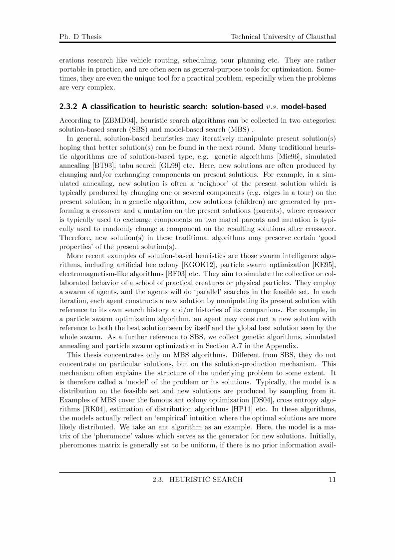
This thesis concentrates only on MBS algorithms. Different from SBS, they do notconcentrate on particular solutions, but on the solution-production mechanism. Thismechanism often explains the structure of the underlying problem to some extent. Itis therefore called a ‘model’ of the problem or its solutions. Typically, the model is adistribution on the feasible set and new solutions are produced by sampling from it.Examples of MBS cover the famous ant colony optimization [DS04], cross entropy algo-rithms [RK04], estimation of distribution algorithms [HP11] etc. In these algorithms,the models actually reflect an ‘empirical’ intuition where the optimal solutions are morelikely distributed. We take an ant algorithm as an example. Here, the model is a ma-trix of the ‘pheromone’ values which serves as the generator for new solutions. Initially,pheromones matrix is generally set to be uniform, if there is no prior information avail-
2.3. HEURISTIC SEARCH 11

Ph. D Thesis Technical University of Clausthal
able. This will result in a purely random search in the first iteration. This reflects aninitial intuition that every feasible solution is possible to be an optimal solution beforeevaluation. After several iterations, the matrix has been empirically updated (typicallybiased to some best solutions seen), it is now no longer uniform. The resulted search ispossibly biased to a particular area on the solutions space. Now, it reflects an experi-enced intuition that the optimal solutions are more likely distributed in some particulararea.
Generally, model-based search will iteratively evolve models. In each iteration, theysample some solutions from the present model. Then, an empirical model will be learnedfrom some selected ‘best’ solutions in the present sample and/or history. These solutionsare typically selected based on their qualities. Hence, the learned model may concentrateon some good solutions. The model for next iteration is eventually constructed withreference to the present model and the learned empirical model. It is therefore biased togood solutions. So, we may expect that in the next sampling, more good solutions willbe generated.
A common motivation in MBS is to reach a model which can concentrate only onoptimal solutions. To achieve this, they often specify a family of candidate models. Andthe evolution is generally restricted in that family. Model-based search actually resultin a search in the model family. They hope they can reach an ‘optimal’ model i.e. amodel producing optimal solutions only or with an overwhelming probability. Therefore,intrinsically MBS optimize models. This is the most significant difference from SBS.
To further understand MBS, we will collect some popular MBS algorithms in practicein Chapter 3.
2.3. HEURISTIC SEARCH 12
3 A short tutorial on model-based searchalgorithms used in practice
As a background, we have briefly introduced CO (combinatorial optimization) andheuristic search in last Chapter. From now on, we shall concentrate on our main topic:MBS i.e. model-based search (heuristics). This Chapter shall serve as a (short) tutorialfor those MBS algorithms used in practice.
MBS algorithms have been applied successfully to many very tough COPs. Forexample, traveling salesman problem, see [DBKMR05], [Rub99], [DMC96], [DG97b],[OHS+11] etc; maximal cut problem, see [Rub02], [LDM09] etc; vehicle routing prob-lem, see [CHdM05], [BHS99] etc; traffic assignment problem e.g. [ML09]; job shopscheduling, see [SBW11], [CDMT94] etc; buffer allocation e.g. [AKRR05]. According totheir originations, MBS algorithms in practice can be collected in three classes: cross en-tropy algorithms [RK04], ant colony optimization [DS04] and estimation of distributionalgorithms [HP11].
Cross entropy algorithm (CE) was initially motivated for rare event simulation, see[Rub97], [Rub99] or A.6 in Appendix. It can be strictly derived by importance samplingunder the so-called Kullback-Leibler divergence, see [Rub99]. It has many variants avail-able in the literature, see e.g. [Rub99], [CJK07], [Mar05], [WK14b]. In this Chapter, wewill concentrate on the initial version presented in [Rub99]. However, as a reference, wewill also make a very short introduction to the additional features in its variants.
Ant colony optimization (ACO) is a large class of algorithms which mimics the foragingbehavior of a colony of real ants, see [DS04] for an overview. In this Chapter, we con-centrate only on four representative algorithms, namely ant system (AS, see [DMC96]),ant colony system (ACS, see [DG97b]),MAX -MIN ant system (MMAS, see [SH00])and population-based ant system (PBAS, see [GM02]). We formally define these fouralgorithms. As a useful reference, we also describe the foraging behavior of real ants.
Estimation of distribution algorithms (EDA, see [HP11]) is a common name for manyalgorithms which were initially motivated for efficiently simulating genetic algorithms byprobabilistic models. According to the employed models, estimation of distribution algo-rithms can be collected in two classes: algorithms with univariate marginal models andalgorithms with multivariate marginal models. Here, univariate marginal models are dis-tributions with independent marginals, and multivariate marginal models are those withdependent marginals. Algorithms with univariate marginal models are e.g. univariatemarginal distribution algorithm (UMDA, see [MP96]), the population based incrementallearning (PBIL, see [Bal94]), and the compact genetic algorithm (CGA, see [HLG99]).Algorithms with multivariate marginal models are e.g. Bayesian optimization algorithm(BOA, see [HGC95], [PM98], [PGCP00], [PGL02], [Pel05]), bivariate marginal distribu-
13
Ph. D Thesis Technical University of Clausthal
tion algorithm (BMDA, see [MP96]), mutual information maximizing input clustering(MIMIC, see [DBIV+97]) and extended compact genetic algorithm (ECGA, see [SG00]).Generally, it is difficult to apply an algorithm with multivariate marginal models to op-timization problems in practice. The main reason is that learning a multivariate modelitself may require a lot of computational effort. Therefore, we will concentrate only onalgorithms with univariate marginal models.
The whole Chapter is arranged as: Section 3.1 formalize a common motivation forthese algorithms; Section 3.2 introduces the cross entropy algorithms; Section 3.3 intro-duces the ant colony optimization algorithms; Section 3.4 introduces the estimation ofdistribution algorithms.
3.1 A common motivation
As mentioned in Section 2.3.2, MBS algorithms do not concentrate on particular so-lutions, but on models. Here, a model is a mechanism which can be used to produce(random) solutions for a CO instance. Generally, it can be expressed as a finite list ofparameters, namely a finite vector of reals, due to the finiteness of the underlying feasibleset. Typically, it is a distribution1 on the underlying feasible set, and new solutions aregenerated by sampling.
MBS algorithms often restrict their models in a specified family. A common motivationhere is that they want to find out an ‘optimal’ model from that family which may produceoptimal solutions only (or with an overwhelming probability). To achieve this, they mayarbitrarily fix an initial model in that family, and then iteratively evolve the model inthe specified family by some fixed strategies. Intrinsically, they optimize models or thesolution-production mechanism.
Assume that (S, f, 0) is the underlying CO instance. Let P be a specified family ofmodels on S satisfying the basic requirement that
there exists Π∗ ∈ P : Π∗ only produces optimal solutions (3.1)
where S∗ is the collection of optimal solutions. And we denote the collection of models∈ P which satisfies (3.1) as P∗. Obviously, ∅ 6= P∗ ⊆ P under condition (3.1). Then, thecommon motivation of MBS can be formally stated as an ‘optimization’ task picking outan ‘optimal model’ Π∗ ∈ P∗ from candidates ∈ P.
To do that, these algorithms generally employ a stochastic search on P. Let Π0 ∈ Pbe an arbitrarily fixed initial model. They then iteratively evolve their models throughthe following three phases:
1See A. 5 in the Appendix for a formal definition of distributions.
3.1. A COMMON MOTIVATION 14

Ph. D Thesis Technical University of Clausthal
Crude MBS procedure
Sampling: draw a sample Xt of a specified size from current model Πt ∈ P;
Learning: learn an empirical model Wt ∈ P from some ‘best’ solutions in Xt
and/or in past iterations, by a specified learning rule;
Update: construct a new model Πt+1 ∈ P with reference to the present modelΠt and the empirical model Wt, by a specified update rule.
Here, Wt is a model concentrating on some ‘best’ solutions seen currently and/or in thepast. With reference to Wt, the next model Πt+1 can be biased to ‘good solutions’.Thereby, we may expect that more good solutions will be produced in the next round.
Along with MBS algorithms, it is an iteratively single-start ‘local’ search procedure onthe specified model family P. Here, ‘single-start’ means that we start from a single modeland construct only one model for the next round (namely Πt+1) in each iteration. Withword ‘local’, we mean that Πt+1 is actually a ‘neighbor’ of Πt since it is constructed alsowith reference to Πt. It may not be ‘far’ way from Πt on the space P. This ‘localism’can make the movement of models smoothly on the P. It actually reflects a underlyingconservatism. We hope that Πt+1 can assimilate the good information concealing inWt, but we may not hope that Πt+1 is completely a copy of Wt. Otherwise, it may bevery difficult for the algorithm to escape from the local trap which may be formed byWt. In the remaining of this Chapter, we will further understand the motivation andthis underlying search on P through some MBS algorithms used in practice.
3.1. A COMMON MOTIVATION 15

Ph. D Thesis Technical University of Clausthal
3.2 Example I: cross entropy algorithm
Cross entropy algorithm (CE) is a very typical MBS algorithm. It was invented byR.Y. Rubinstein, see [Rub99]. Initially, it was motivated for rare-event simulation incomplex network simulation, see [Rub97] or A. 6 in the Appendix. Then it was realizedas a good and generic optimization tool for both continuous and discrete optimization,see [Rub99]. For a detailed book on CE in CO, see [RK04]. For a concise and helpfultutorial, see [DBKMR05]. There are also several CE variants available in the literature,see e.g. [RK04], [Mar05], [CJK07] and [WK14b]. Here, we stick on the original CEversion presented in [Rub99]. As a reference, we shall also make a short introduction tothe additional features in its variants.
3.2.1 Representation of feasible solutions
Recall that MBS algorithms optimize models instead of solutions. And the models arerestricted in a specified family. In CE, models are actually distributions on the underlyingfeasible set. To explicitly express the models in CE, we need to formalize the feasiblesolutions.
Without loss in generality, we assume here a minimizing CO instance (S, f, 0). Notethat any maximizing instance can be easily translated into a minimizing instance. Forexample, let (S′, f ′, 1) be an maximizing instance, then (S′,−f ′, 0)2 is an minimizinginstance which has the same feasible set and optimal solutions as (S′, f ′, 1).
In CE, feasible solutions are often assumed to be fixed length strings over a finitealphabet3, see e.g. [Rub99], [CJK07], [WK14b]. This is reasonable. Actually, for eachCO instance, we can represent its feasible solutions in this fashion, due to finiteness ofits feasible set. We take an MaxCut (Maximal Cut, see Subsection 2.2.3) instance asan example. Here, a cut (V1, V2) on the underlying graph is a partition for the verticesV . Let n denote the size of V. Then, a cut can be uniquely represented as a string(b1, . . . , bn) of length n over the alphabet 0, 1, if we employ a rule (encoding) that
bi =
0 if the i-th vertex ∈ V1,
1 otherwise,
for each i = 1, . . . , n. Therefore, we now think that each feasible solution s ∈ S of theunderlying instance is a string (a1, . . . , aL) where each item ai ∈ A for i = 1, . . . , L, Ais a finite alphabet and L ∈ N is a fixed solutions length. Obviously, S ⊆ AL.
Generally, CE may further assume that S = AL, see e.g. [DBKMR05] and [CJK07].Here, we follow this assumption too. Of cause, it may occur that S 6= AL in practice.If this is the case, we can assign a penalty objective value to those infeasible strings soas to make all strings in AL ‘feasible’. We can employ an arbitrary value vmax as thepenalty value where
vmax > fmax = maxf(s)
∣∣ s ∈ S.2Here, −f ′ is a function defined as −f ′(s) = −1 · f(s) for each s ∈ S′.3An alphabet is a set of items, typically these items are letters.
3.2. EXAMPLE I: CROSS ENTROPY ALGORITHM 16

Ph. D Thesis Technical University of Clausthal
Then, (S, f, 0) can be extended into an CO instance (AL, f ′, 0) with
f ′(s) =
f(s) if s ∈ S,vmax otherwise i.e. s is infeasible.
We can equivalently solve (AL, f ′, 0) instead of (S, f, 0).
3.2.2 The specified model family for cross entropy algorithm
With the above representation i.e. S = AL for some finite A and L ∈ N, we are nowready to show the commonly used models in CE. Let P(A) be the class of all possibledistributions on the alphabet A for the underlying instance (S, f, 0). Obviously, eachπ ∈ P(A) can be represented as a vector of length |A| over R+ ∪ 0, i.e.
π =(π(a)
)a∈A with each π(a) ≥ 0 and
∑a∈A
π(a) = 1.
It describes a mechanism for producing random items or letters fromA. We define furtherthat
Pce := P(A)× P(A)× · · · × P(A) = P(A)L. (3.2)
Generally, CE algorithms specify Pce as the model family.Obviously, each model Π =
(Π(1), . . . ,Π(L)
)∈ Pce with each Π(i) ∈ P(A) is a
product distribution on the product space AL = A × · · · × A. And a random strings = (a1, . . . , aL) ∈ AL is then sampled with a probability
Π(s) =L∏i=1
Π(i)(ai),
where observe that Π(i) =(Π(i)
(a))
a∈A∈ P(A), for each i = 1, . . . , L, describing a
selection in the collection A. Of cause, Π can also be written in details as a vector ofreals
Π =(Π(i)
)i=1,...,L
=(Π(a; i)
)a,∈A;i=1,...,L
with Π(a; i) := Π(i)(a).
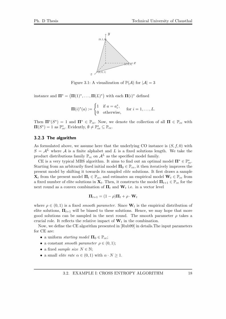
Actually, P(A) is a closed continuous space i.e. it can be identified as a closed con-tinuous region on the Euclidean Space Rn where n = |A|. For example, when |A| = 3,P(A) can visually drawn as the gray triangular on Figure 3.1. Since Pce = P(A)L withL < ∞, Pce is then also continuous. Moreover, Pce is closed under limits i.e. for anyconvergent sequence
(Πm
)m∈N with each Πm ∈ Pce, we have
limm→∞
Πm ∈ Pce.
It is not difficult to see that the family Pce satisfies the basic requirement (3.1) forMBS model family. Let s∗ = (a∗1, . . . , a
∗L) ∈ S∗ be an optimal solution of the underlying
3.2. EXAMPLE I: CROSS ENTROPY ALGORITHM 17
Ph. D Thesis Technical University of Clausthal
x(1, 0, 0)
y
(0, 1, 0)
z(0, 0, 1)
Figure 3.1: A visualization of P(A) for |A| = 3
instance and Π∗ =(Π(1)∗, . . . ,Π(L)∗
)with each Π(i)∗ defined
Π(i)∗(a) :=
1 if a = a∗i ,
0 otherwise,for i = 1, . . . , L.
Then Π∗(S∗) = 1 and Π∗ ∈ Pce. Now, we denote the collection of all Π ∈ Pce withΠ(S∗) = 1 as P∗ce. Evidently, ∅ 6= P∗ce ⊆ Pce.
3.2.3 The algorithm
As formulated above, we assume here that the underlying CO instance is (S, f, 0) withS = AL where A is a finite alphabet and L is a fixed solutions length. We take theproduct distributions family Pce on AL as the specified model family.
CE is a very typical MBS algorithm. It aims to find out an optimal model Π∗ ∈ P∗ce.Starting from an arbitrarily fixed initial model Π0 ∈ Pce, it then iteratively improves thepresent model by shifting it towards its sampled elite solutions. It first draws a sampleXt from the present model Πt ∈ Pce, and estimates an empirical model Wt ∈ Pce froma fixed number of elite solutions in Xt. Then, it constructs the model Πt+1 ∈ Pce for thenext round as a convex combination of Πt and Wt i.e. in a vector level
Πt+1 = (1− ρ)Πt + ρ ·Wt
where ρ ∈ (0, 1) is a fixed smooth parameter. Since Wt is the empirical distribution ofelite solutions, Πt+1 will be biased to these solutions. Hence, we may hope that moregood solutions can be sampled in the next round. The smooth parameter ρ takes acrucial role. It reflects the relative impact of Wt in the combination.
Now, we define the CE algorithm presented in [Rub99] in details.The input parametersfor CE are:
• a uniform starting model Π0 ∈ Pce;• a constant smooth parameter ρ ∈ (0, 1);
• a fixed sample size N ∈ N;
• a small elite rate α ∈ (0, 1) with α ·N ≥ 1.
3.2. EXAMPLE I: CROSS ENTROPY ALGORITHM 18

Ph. D Thesis Technical University of Clausthal
CE strictly obeys the crude MBS procedure described on p. 15. The three phases herecan be defined in details as following.
Algorithm: cross entropy
Sampling: We generate a random sample Xt =(X
(1)t , . . . ,X
(N)t
)from the present
model Πt =(Πt(i)
)i=1,...,L
∈ Pce. Here, each X(j)t is a random string in AL
and can be represented in details as(X
(j)t (1),X
(j)t (2), . . . ,X(j)(L)
)where each X
(j)t (i) is a random item in A chosen independently by Πt(i) for
i = 1, . . . , L.
Learning: We calculate the objective values of the sampled solutions in Xt, andorder them as
f(X(n1)t ) ≤ f(X
(n2)t ) ≤ · · · ≤ f(X
(nN )t ).
We pick out the best bα ·Nc solutions and collect them in N bt i.e.
N bt =
X
(n1)t , . . . ,X
(nbα·Nc)t
where α ∈ (0, 1) is the fixed elite rate. For each item a ∈ A and positioni ∈ 1, . . . , L, we calculate a relative frequency Wt(a; i) in the elite solutionsN bt as
Wt(a; i) :=
∑bαNcj=1 1a
(X
(nj)t (i)
)bαNc . (3.3)
And then, we collect all these frequencies in
Wt :=(Wt(1), . . . ,Wt(L)
)=(Wt(a; i)
)a∈A;i=1,...,L
(3.4)
with each Wt(i) :=(Wt(a; i)
)a∈A for i = 1, . . . , L.
Update We construct the next model Πt+1 as a convex combination of Πt and Wt
i.e.Πt+1 = (1− ρ)Πt + ρWt (3.5)
In details,Πt+1(a; i) = (1− ρ)Πt(a; i) + ρWt(a; i) (3.6)
for each a ∈ A and i = 1, . . . , L.
To make the above algorithm more clearly, a pseudo code is listed in Figure 3.2 on p.22.
Note that, each Wt(i) =(Wt(a; i)
)a∈A in the above algorithm is actually a distribu-
3.2. EXAMPLE I: CROSS ENTROPY ALGORITHM 19

Ph. D Thesis Technical University of Clausthal
tion on A, since
∑a∈A
Wt(a; i) =∑a∈A
∑bαNcj=1 1a
(X
(nj)t (i)
)bαNc =
∑bαNcj=1
∑a∈A 1a
(X
(nj)t (i)
)bαNc
=
bαNc∑j=1
1
bαNc = 1.
Thereby,Wt =
(Wt(1), . . . ,Wt(L)
)=(Wt(a; i)
)a∈A;i=1,...,L
is a model in Pce. Actually, Wt maximizes the likelihood function of elite solutions N bt
i.e. it maximizesbα·Nc∑j=1
lnW(X(nj)t ) for W ∈ Pce. (3.7)
Moreover, it is also the model in Pce which is closest to the truncate distribution
W∗t (s) =
1s′∈S|f(s′)≤γt(s)Πt(s)∑s′′∈S 1s′∈S|f(s′)≤γt(s
′′)Πt(s′′)for each s ∈ S (3.8)
under the so-called Kullback-Leibler distance (see A. 2 in the Appendix) where γt =
f(X
(nbα·Nc)t
), see [Rub99] for a proof.
Since Wt ∈ Pce and Πt ∈ Pce, Πt+1 is also a model in Pce under update (3.5) and(3.6). And since Wt approximates the truncate distribution (3.8), Πt+1 is biased tothe solutions having objective value smaller than γt. Thereby, we can hope that moresolutions of objective value smaller than γt can be sampled in the next round. Thesmooth parameter ρ reflects the relative importance of the empirical distribution Wt inthe update (3.5). It almost dominates the asymptotic behavior of CE, for details see[WK14b].
The algorithm actually results in a random walk on the continuous space Pce. We startfrom an initial model (uniform) Π0 ∈ Pce. And in each subsequent iteration, we movethe present model Πt to a ‘neighbor’ Πt+1. The move is made smoothly through theupdate (3.5). The neighbor Πt+1 is constructed in a way that it not only preserves some‘local’ information in Πt with a rate 1− ρ, but also assimilates some ‘elite’ information(note that Wt is an approximation of (3.8)) with a rate ρ.
3.2.4 A brief introduction to CE variants
There are also some CE variants, e.g. CE with time-dependent smooth parameters(CE/tdsp, [CJK07]), Ant-like CE (CE/ant, [WK14b]), fully adaptive CE (FACE, [RK04]),graph-based CE with time-dependent smooth parameters (GBCE/tdsp, [Mar05]) andgraph-based CE with lower bound on distributions (GBCE/lb, [Mar05]). The essentialfeatures of these algorithms are covered in the defined CE. Now we make an introductionto their additional features.
3.2. EXAMPLE I: CROSS ENTROPY ALGORITHM 20

Ph. D Thesis Technical University of Clausthal
The unique additional feature in CE/tdsp is that it does not employ a fixed smooth pa-rameter, but a sequence of smooth parameters
(ρt)t≥1
. And the update (3.5) is thereforechanged to
Πt+1 = (1− ρt+1)Πt + ρt+1Wt
where Πt is the present model and Wt is calculated by (3.3) and (3.4). Ant-like CE isan extension of CE/tdsp. It introduces a ‘feasibility distribution’ concept into the above‘Sampling’ phase. This concept is inspired by the so-called ‘visibility’ in ant colonyoptimization. In the next Chapter, we shall formally introduce this. GBCE/tdsp is avariant of CE/tdsp. It estimates Wt only from the best solution found in history.
The additional feature in FACE is that it does not fix the sample size. It allows thesample size to vary within a fixed range. In the end of each iteration, it sets the nextsample size based on N b
t . In other word, it employs dynamic sample size.GBCE/lb is a variant mimicking MAX -MIN ant system. It introduces a constant
lower bound pmin to restrict each entry Πt+1(a; i) in Πt+1 after the update (3.5) i.e. ifΠt+1(a; i) < pmin, set Πt+1(a; i) = pmin.
3.2. EXAMPLE I: CROSS ENTROPY ALGORITHM 21
Ph. D Thesis Technical University of Clausthal
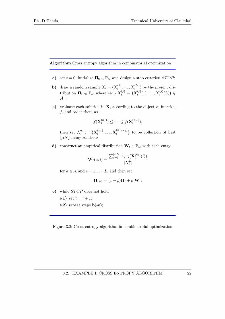
Algorithm Cross entropy algorithm in combinatorial optimization
a) set t = 0, initialize Π0 ∈ Pce and design a stop criterion STOP ;
b) draw a random sample Xt = (X(1)t , . . . ,X
(N)t ) by the present dis-
tribution Πt ∈ Pce where each X(j)t =
(X
(j)t (1), . . . ,X
(j)t (L)
)∈
AL;
c) evaluate each solution in Xt according to the objective functionf, and order them as
f(X(n1)t ) ≤ · · · ≤ f(X
(nN )t ),
then set N bt := X(n1)
t , . . . ,X(nbαNc)t to be collection of best
bαNc many solutions;
d) construct an empirical distribution Wt ∈ Pce with each entry
Wt(a; i) =
∑bαNcj=1 1a
(X
(nj)t (i)
)|N b
t |
for a ∈ A and i = 1, . . . , L, and then set
Πt+1 = (1− ρ)Πt + ρ Wt;
e) while STOP does not hold
e 1) set t = t+ 1;
e 2) repeat steps b)-e);
Figure 3.2: Cross entropy algorithm in combinatorial optimization
3.2. EXAMPLE I: CROSS ENTROPY ALGORITHM 22

Ph. D Thesis Technical University of Clausthal
3.3 Example II: ant colony optimization
Ant colony optimization (ACO) is a large class of MBS algorithms which mimics theforaging behavior of a colony of real ants, see [DS04] and [DS10] for an overview. Here,we concentrate on four representative ACO algorithms: ant system, ant colony system,MAX -MIN ant system and population-based ant system. For a reference of otherACO algorithms, see [DS04].
A(20)
C(0)
B(0)
d = 1, τ = 1 10 ants
d = 1, τ = 1
d = 1, τ = 110 ants
(a) t = 0
A(0)
C(10)
B(10)
τ = 0
τ = 0 10 ants
τ = 010 ants
(b) t = 1
A(10)
C(0)
B(10)
τ = 0
τ = 0 10 ants
τ = 910 ants
(c) t = 2
A(0)
C(10)
B(10)
τ = 0 10 ants
τ = 9
τ = 810 ants
(d) t = 3
A(20)
C(0)
B(0)
τ = 9 7 ants
τ = 8
τ = 1713 ants
(e) t = 4
Figure 3.3: A demo of ants foraging behavior
3.3.1 The foraging behavior of ants
ACO algorithms are inspired by the foraging behavior of real ants. Hence, it is helpfulto understand this behavior before formally introducing them. Figure 3.3 above clearlydemonstrates the foraging behavior.
In practice, ants use a substance called ‘pheromone’ as a medium to communicatewith each other in foraging. When an ant finds a food source, it will deposit pheromoneson its way back to the nest. Other ants can detect the deposited pheromones, and thehigher the pheromones on a way the more possible they may follow. The pheromonesdeposited on a way may also evaporate with a certain speed. These can help the antsquickly find and concentrate on a nearest path from their nest to a food source. Figure3.3 depicts five instants in the foraging procedure for a colony of 20 ants. Here, weassume a nest A, a food source B, and two possible paths from the nest to the uniquefood source i.e. A − C − B and A − B. On the Figure, we use d and τ to describe the
3.3. EXAMPLE II: ANT COLONY OPTIMIZATION 23

Ph. D Thesis Technical University of Clausthal
distance and the value of pheromones respectively, e.g. in Subfigure 3.3a we write d = 1and τ = 1 on each edge to mean that the edges are of the same length and the sameinitial pheromones value. The number inside a bracket following the label of a noderepresents the number of ants positioned in that node at the corresponding time. Forexample, in Subfigure 3.3a (t=0) we use A(20) to mean that all ants are positioned innode (nest) A at t = 0.
Initially (t = 0, Subfigure 3.3a), all ants are positioned in node (nest) A. Since wedeposit the same initial pheromones on edges A − C and A − B, one half of the antswill follow A− C and others will follow A−B in expectation, see the dashed arrow onSubfigure 3.3a.
At time t = 1 (Subfigure 3.3b), 10 ants stand in node C and other 10 ants stand infood source B, where observe that A − C and A − B have the same length, and weassume that all the ants walk with the same speed. Here, we also assume that in 1 unittime, the pheromones on each edge will evaporate 1 unit. So, the pheromones value foreach edge at time t = 1 equals 0. The ants which has reached food source at t = 1 willreturn back to the nest and deposit pheromones on the path they found i.e A−B. Otherants (those in C) will continue to search for a source.
At t = 2 (Subfigure 3.3c), 10 ants returned the nest A from the source B, and 10reached the source B from the node C. Here, we assume that each ant deposits 1 unitof pheromones to each edge on its way back. Thereby, the pheromones value on A−Bnow is 9 units, where 10 units of pheromones are deposited by the 10 returned ants,but 1 unit of pheromones evaporated. The returned ants (those in the nest A) will stillfollow path A− B in the next round, because the pheromones value on A− C is 0 (bythe evaporation) while the pheromones values on A−B is 9. And those ants arrived insource B will return back and deposit pheromones on the path they found i.e. A−C−B.
At t = 3 (Subfigure 3.3d), the pheromones value on C − B is 9 i.e. 10 units aredeposited by the returned ants and 1 unit evaporated. And now there are again 10 antsin source B and 10 ants in C. And the ants in source B will again go back to nest Aalong path A−B, since this is still the path they found in this round.
At t = 4 (Subfigure 3.3e), all the ants returned in nest A, and now the pheromonesvalues on A − B and A − C are 17 units and 9 units respectively. Therefore, we canexpect that 7 ants ( 9
26 · 20 ≈ 6.92) will follow A−C and 13 ants will follow A−B in thenext round i.e. the majority of the ants will follow the shorter path A − B when theyall completed round trips.
Figure 3.3 actually depicts an ant cycle for that colony of 20 ants. Here, an ant cyclemeans a time interval in which all the ants started simultaneously from their nest andcompleted at least one round trip between their nest and a food source, and at leastone ant finished only one round trip. Since the length of path A − B is 1 unit and thelength of path A−C−B is 2 units, the ants following A−B can finish two round trips,but those following A−C −B finish only one round trip in this cycle. As a result, antsdeposited totally 20 units of pheromones on A − B, but only 10 units on A − C andC−B i.e. the amount of pheromones deposited by ants are proportional to the qualitiesof the paths (reciprocal of the path length). Due to evaporation, in the end of this cyclethe remained pheromones on A − B, A − C and C − B are 17, 9, 8 units respectively.
3.3. EXAMPLE II: ANT COLONY OPTIMIZATION 24

Ph. D Thesis Technical University of Clausthal
The shorter path (i.e. A − B) is therefore overwhelmingly attractive in the next cycle.ACO algorithms would use this behavior as a basic idea in solving practical problems.They see each iteration as an ant cycle, collect the pheromones on edges in a matrixas the ‘model’ for producing random solutions. Here, a random solution is generatedin a way analogous to the construction of a path by an ant in the foraging. And thepheromones matrix is also updated in a similar way as what the ants and evaporationdo in the foraging.
3.3.2 Representation of solutions: walks on a construction graph
To apply the foraging behavior, we first need to construct a graph for the underlyingCO instance such that each feasible solution can be represented as a walk on that (con-struction) graph. Here, a graph G (see also A. 1 in the Appendix) is a pair (V,E) whereV is a finite set of vertices and E ⊆ (v1, v2) | v1 ∈ V, v2 ∈ V . And a walk W on G is asequence v1, (v1, v2), v2, (v2, v3), v3, . . . , (vk−1, vk), vk such that
• vi ∈ V for each i = 1, . . . , k,
• each pair (vi, vi+1) ∈ E for i = 1, . . . , k − 1.
Obviously, walk W can be identically represented as a string of vertices v1, v2, . . . , vk. IfE satisfies that
∀v1 ∈ V and v2 ∈ V (v1, v2) ∈ E ⇒ (v2, v1) ∈ E,
we call G as a undirected graph and each pair in E as an edge. Otherwise, we call eachpair in E as an arc and the graph as a directed graph. Figure 3.4 below shows examplesof an undirected graph and a directed graph. Here, two graphs have the same verticesV = v1, v2, v3, v4, an edge is drawn as a line (Subfigure 3.4a) and an arc is drawn asa line with arrow (Subfigure 3.4b).
v1 v2
v3v4
(a) undirected graph
v1 v2
v3v4
(b) directed graph
Figure 3.4: Examples of graphs
Formally, we say that a (directed) graph G = (V,E) is a construction graph for a COinstance (S′, f ′, 0) (similarly for the maximizing case) under map Φ if (see also Definition3.1 in [Gut00])
• there is a unique vertex v0 ∈ V which is marked as a starting vertex ;
• let W be the collection of those walks W satisfying the following conditions
a) W starts at v0,
b) W traverses (contains) each vertex at most once,
3.3. EXAMPLE II: ANT COLONY OPTIMIZATION 25

Ph. D Thesis Technical University of Clausthal
c) let e be the end vertex of W, then
∀v ∈ V : (e, v) ∈ E ⇒ v has been traversed by W,
d) Φ : S′ 7→ W is a bijection4.
Let G = (V,E) be a construction graph for a CO instance (S′, f ′, 0). We shall call eachwalk on G satisfying a)-c) as a legal walk to that instance. By condition b), a legal walkcan contain at most |V | <∞ many vertices. And by condition c), a legal walk can not becontinued without conflicting condition b). For example, there are only two legal walkson Subfigure 3.4b (v1, v2, v3, v4) and (v1, v3, v4) where we identify v1 as the start vertex.Although (v1, v2), (v1, v2, v3) and (v1, v2, v3, v2) are walks, they conflict either conditionb) or condition c).
In practice, it may be convenient for us to represent a CO instance through a graph.Typical examples are those tour planning problems in Operations Research like TSP.Here, we can arbitrarily fix a starting vertex, and then a legal walk is a walk whichstarts from the starting vertex and traverses all vertices exactly once. Actually, for anarbitrary CO instance it is also possible for us to construct a graph although this may notbe efficient. Let (S′′, f ′′, 0) be an arbitrary instance, we can define a graph G = (V,E)that V = S′′
⋃♣ and E = (♣, s) | s ∈ S′′ where ♣ /∈ S′′ is a symbol. Then G is aconstruction graph for (S′′, f ′′, 0) with the unique starting vertex ♣.
Now, we introduce some auxiliary definitions and notations related to constructiongraph. We call a walk on a construction graph G which satisfies conditions a)-b) as apartial legal walk. Let y = (v0, v1, . . . , vn) be a partial legal walk, then we shall useVFeasible(y) to notate the collection of all the vertices v ∈ V making (v0, . . . , vn, v) a newpartial legal walk. Of cause, VFeasible(y) = ∅ implies y is a (completed) legal walk. Andwe shall refer to each vertex in VFeasible(y) as a feasible continuation to walk y providedVFeasible(y) 6= ∅.
In the sequel of this Section, we assume without loss in generality that the underlyingCO instance is an minimizing instance with objective function f and feasible set S =Wwhere W is the collection of legal walks on a construction graph G = (V,E). And weassume further that v0 is the unique start vertex on G for all legal walks.
3.3.3 Ant System: the first ACO algorithm
Now, we are ready to formally define ACO algorithms. Here, we start with ant system.Ant system (AS), see [DMC96], is the first ACO algorithm. It completely mimics theant foraging behavior. Other ACO algorithms can be seen as variants of this algorithm.
The definition of ant system
AS employs a fixed number of artificial ants to iteratively construct random walks onthe underlying graph G = (V,E), and the corresponding search mimics completely theforaging behavior. AS identifies v0 (the start vertex) as the unique nest for those artificial
4A bijection g : A 7→ B is an injection such that for any y ∈ B there is an x ∈ A with y = g(x)
3.3. EXAMPLE II: ANT COLONY OPTIMIZATION 26

Ph. D Thesis Technical University of Clausthal
ants. And an iteration is seen as an ant cycle. The difference here is that each artificialant may walk on G only once in each cycle. Initially, a fixed amount of pheromones isdeposited on each arc ∈ E. And in each cycle (iteration), all the (artificial) ants startfrom the fixed nest (i.e. v0) and independently construct (random) legal walks. Whenan ant finished a partial legal walk, it may choose a feasible continuation according to aprobability proportional to the present pheromones. After all ants completed their (legal)walks, the objective values of the walks are calculated, and the present pheromones oneach arc ∈ E evaporate with a fixed rate (i.e. evaporation rate). Finally, each antdeposits an amount of new pheromones on arcs it traversed in this cycle and the amountis based on the qualities of the constructed walk i.e. the better the walk the morepheromones it deposits. Here, the end vertex of a legal walk is thought as a food sourceand the objective value is seen as the distance from the nest to that source.
Generally, AS takes four input parameters:
• a fixed number N ∈ N of artificial ants;
• a fixed evaporation rate ρ ∈ (0, 1);
• a constant initial pheromones value c0 > 0 for each arc ∈ E;
• a positive decreasing assessment function g : R 7→ R+.
Then each of its iterations can be formally defined as following, where we use τt(a, b) torepresent the pheromones value on arc (a, b) ∈ E in iteration t ∈ N and τ0(a, b) = c0 foreach arc (a, b) ∈ E.
In the below algorithm, legal walks may be of a different length i.e. may containdifferent number of vertices. Therefore, we use nj to represent the number of verticescontained in the j-th legal walk in an iteration. Note that, this nj is a variable, becausethe j-th legal walks in different iterations may have different numbers of vertices.
3.3. EXAMPLE II: ANT COLONY OPTIMIZATION 27
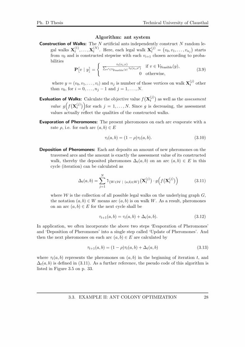
Ph. D Thesis Technical University of Clausthal
Algorithm: ant system
Construction of Walks: The N artificial ants independently construct N random le-
gal walks X(1)t , . . . ,X
(N)t . Here, each legal walk X
(j)t =
(v0, v1, . . . , vnj
)starts
from v0 and is constructed stepwise with each vi+1 chosen according to proba-bilities
P[v | y
]=
τt(vi,v)∑
v′∈VFeasible(y)τt(vi,v′)
if v ∈ VFeasible(y),
0 otherwise,(3.9)
where y = (v0, v1, . . . , vi) and nj is number of those vertices on walk X(j)t other
than v0, for i = 0, . . . , nj − 1 and j = 1, . . . , N.
Evaluation of Walks: Calculate the objective value f(X
(j)t
)as well as the assessment
value g(f(X
(j)t
))for each j = 1, . . . , N. Since g is decreasing, the assessment
values actually reflect the qualities of the constructed walks.
Evaporation of Pheromones: The present pheromones on each arc evaporate with arate ρ, i.e. for each arc (a, b) ∈ E
τt(a, b) = (1− ρ)τt(a, b). (3.10)
Deposition of Pheromones: Each ant deposits an amount of new pheromones on thetraversed arcs and the amount is exactly the assessment value of its constructedwalk, thereby the deposited pheromones ∆t(a, b) on an arc (a, b) ∈ E in thiscycle (iteration) can be calculated as
∆t(a, b) =N∑j=1
1W∈W | (a,b)∈W(X
(j)t
)· g(f(X
(j)t
))(3.11)
where W is the collection of all possible legal walks on the underlying graph G,the notation (a, b) ∈W means arc (a, b) is on walk W . As a result, pheromoneson an arc (a, b) ∈ E for the next cycle shall be
τt+1(a, b) = τt(a, b) + ∆t(a, b). (3.12)
In application, we often incorporate the above two steps ‘Evaporation of Pheromones’and ‘Deposition of Pheromones’ into a single step called ‘Update of Pheromones’. Andthen the next pheromones on each arc (a, b) ∈ E are calculated by
τt+1(a, b) = (1− ρ)τt(a, b) + ∆t(a, b) (3.13)
where τt(a, b) represents the pheromones on (a, b) in the beginning of iteration t, and∆t(a, b) is defined in (3.11). As a further reference, the pseudo code of this algorithm islisted in Figure 3.5 on p. 33.
3.3. EXAMPLE II: ANT COLONY OPTIMIZATION 28

Ph. D Thesis Technical University of Clausthal
An additional feature for some particular problems: the visibility
In practice, some greedy information for stepwisely constructing a random solution maybe available. To take advantage of these information, AS may add a ‘visibility’ conceptin the above ‘Construction of Walks’.
Now, we employ the famous traveling salesman problem as an example. Assume thatthe underlying graph G = (V,E) is fully connected i.e. E = (a, b) | a ∈ V, b ∈ V , andd : E 7→ R+ is a distance (weighted) function on G. An optimal solution here is just ashortest Hamiltonian circle on G. Note that each Hamiltonian circle actually correspondsto a legal walk on G if we fix a vertex in V as the unique starting vertex v0. Then thecorresponding objective value for a legal walk W = (v0, a1, . . . , an) is
f(W ) = d(v0, a1) +n−1∑i=1
d(ai, ai+1) + d(an, v0)
where we assume further that V = v0, a1, . . . , an for some n ∈ N. Due to the particularform of this objective function, it is reasonable to continue a partial legal walk with amore close feasible continuation. To cover this idea, AS may assume that each artificialants can detect not only the pheromones on an arc but also the length of that arci.e. they can visually compare the distances from their current positions to the feasiblecontinuations by their eyes. Then, an ant can select a feasible continuation according toa mixture of the pheromones and the distances. Formally, the choice probability (3.9)for a feasible continuation therefore becomes
P[v | y
]=
[τt(vi,v)
]α[ 1d(vi,v)
]β∑v′∈VFeasible(y)
[τt(vi,v′)
]α[ 1d(vi,v′)
]β if v ∈ VFeasible(y),
0 otherwise,
(3.14)
where y = (v0, v1, . . . , vi) is partial legal walk with i < n and each vi ∈ V, the VFeasible(y)here is actually V −v0, v1, . . . , vi, d(vi, v) represents the length of arc (vi, v), α > 0 andβ > 0 are two fixed constants reflecting the relative importance of pheromones infor-mation and distances information respectively. We shall refer to (3.14) as the ‘visibilitycase’.
With (3.14) instead of (3.9) in ‘Construction of Walks’, it may result in a dynamicbalance of the empirical information (pheromones) and the prior greedy information(distances). Initially, since pheromones on arcs are of the same value (i.e. τt(a, b) ≡ c0),the distances shall dominate the choice probability (3.14). The algorithm may thereforeperform like a randomized greedy search procedure in an early stage. Hereafter, due tothe accumulated empirical information, the role of the greedy information in (3.14) mayweaken. The underlying search then is guided by a mixture of the empirical and greedyinformation. In our theoretical study, we shall show that the empirical information maygradually dominate the search in a long term.
Similarly, the visibility concept can be carried over to other problems which have asimilar greedy information. Actually, it can be made more extensive so as to captureall problems. However, we shall leave this issue to Section 4.2. In the remaining of this
3.3. EXAMPLE II: ANT COLONY OPTIMIZATION 29
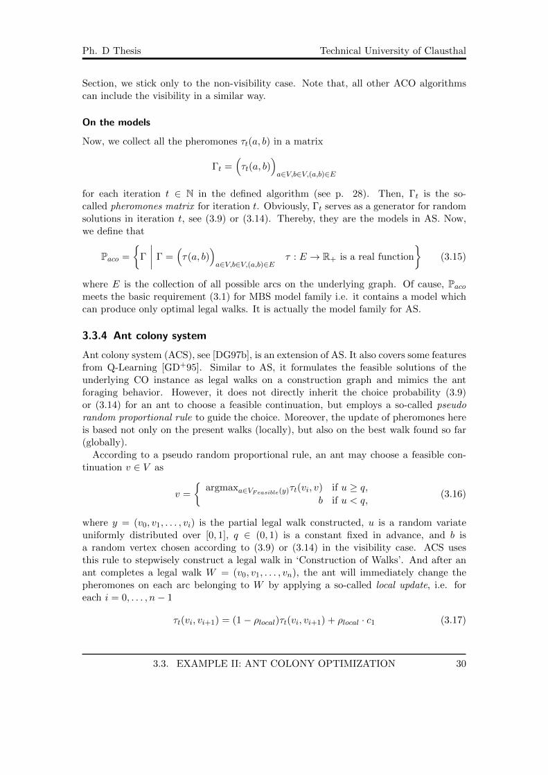
Ph. D Thesis Technical University of Clausthal
Section, we stick only to the non-visibility case. Note that, all other ACO algorithmscan include the visibility in a similar way.
On the models
Now, we collect all the pheromones τt(a, b) in a matrix
Γt =(τt(a, b)
)a∈V,b∈V,(a,b)∈E
for each iteration t ∈ N in the defined algorithm (see p. 28). Then, Γt is the so-called pheromones matrix for iteration t. Obviously, Γt serves as a generator for randomsolutions in iteration t, see (3.9) or (3.14). Thereby, they are the models in AS. Now,we define that
Paco =
Γ
∣∣∣∣ Γ =(τ(a, b)
)a∈V,b∈V,(a,b)∈E
τ : E → R+ is a real function
(3.15)
where E is the collection of all possible arcs on the underlying graph. Of cause, Pacomeets the basic requirement (3.1) for MBS model family i.e. it contains a model whichcan produce only optimal legal walks. It is actually the model family for AS.
3.3.4 Ant colony system
Ant colony system (ACS), see [DG97b], is an extension of AS. It also covers some featuresfrom Q-Learning [GD+95]. Similar to AS, it formulates the feasible solutions of theunderlying CO instance as legal walks on a construction graph and mimics the antforaging behavior. However, it does not directly inherit the choice probability (3.9)or (3.14) for an ant to choose a feasible continuation, but employs a so-called pseudorandom proportional rule to guide the choice. Moreover, the update of pheromones hereis based not only on the present walks (locally), but also on the best walk found so far(globally).
According to a pseudo random proportional rule, an ant may choose a feasible con-tinuation v ∈ V as
v =
argmaxa∈VFeasible(y)τt(vi, v) if u ≥ q,
b if u < q,(3.16)
where y = (v0, v1, . . . , vi) is the partial legal walk constructed, u is a random variateuniformly distributed over [0, 1], q ∈ (0, 1) is a constant fixed in advance, and b isa random vertex chosen according to (3.9) or (3.14) in the visibility case. ACS usesthis rule to stepwisely construct a legal walk in ‘Construction of Walks’. And after anant completes a legal walk W = (v0, v1, . . . , vn), the ant will immediately change thepheromones on each arc belonging to W by applying a so-called local update, i.e. foreach i = 0, . . . , n− 1
τt(vi, vi+1) = (1− ρlocal)τt(vi, vi+1) + ρlocal · c1 (3.17)
3.3. EXAMPLE II: ANT COLONY OPTIMIZATION 30

Ph. D Thesis Technical University of Clausthal
where ρlocal ∈ (0, 1) is a fixed local evaporation rate, and c1 > 0 is a fixed incremental ofpheromones.
After all ants complete their walks, the walks are evaluated and the best found walkXBFt is updated i.e. XBF
t is the best solution among all the walks constructed initerations 0, 1, 2, . . . , t. Then, a global update is applied according to XBF
t , i.e. for anyarc (a, b) ∈ E,
τt+1(a, b) = (1− ρglobal)τt(a, b) + ρglobal∆t(a, b) (3.18)
where ρglobal is a fixed global evaporation rate, and
∆t(a, b) =
g(f(XBF
t ))
if (a, b) ∈ XBFt ,
0 otherwise.(3.19)
with g is a fixed assessment function. See Figure 3.6 on p. 34 for a pseudo code of ACS.
3.3.5 MAX -MIN ant system
MAX -MIN ant system (MMAS), see [SH00], is a variant of AS. Similar to AS, italso employs the choice probability (3.9) or (3.14) (for the visibility case) for an ant tochoose a feasible continuation. However, it employs a fixed upper bound τmax > 0 aswell as a fixed lower bound τmin > 0 to restrict pheromones in each iteration. Moreover,new pheromones are deposited only on those arcs which belongs to the best walk foundor iteration best walk.
In more details, we assume that all ants have completed their walks according to choiceprobability (3.9) or (3.14) in a iteration t i.e. the step ‘Construction of Walks’ on page28. Then all constructed walks are evaluated, and the best found walk XBF
t as well asthe iteration best walk XIT
t are updated i.e. XITt is the best walk among the constructed
walks in the present iteration. To update the pheromones, MMAS randomly choosesa solution Xupd
t from XITt ,XBF
t , and sets τt+1(a, b) for all (a, b) ∈ E as
τt+1(a, b) =
max
(1− ρ)τt(a, b), τmin
if (a, b) /∈ Xupd
t ,
min
(1− ρ)τt(a, b) + ρ · g(f(Xupd
t )), τmax
otherwise.
(3.20)
where ρ ∈ (0, 1) is a fixed evaporation rate, g is a fixed assessment function, τmin > 0and τmax > 0 are fixed pheromones lower bound and upper bound. See Figure 3.7 on p.35 for a pseudo code of MMAS.
3.3.6 Population-based ant system
Population-based ant system (PBAS), see [GM02], is a further variant of MMAS. Itconstructs random solutions (i.e. legal walks) by the same approach as AS andMMAS.And it covers the main feature of MMAS, i,e. it also restricts the pheromones. But ituses a different (pheromones) update mechanism. It does not use evaporation, and onlyrewards the solutions which are stored in an archive. The archive is designed to storeiteration best solutions for some past iterations. Initially, the archive is empty. Then in
3.3. EXAMPLE II: ANT COLONY OPTIMIZATION 31
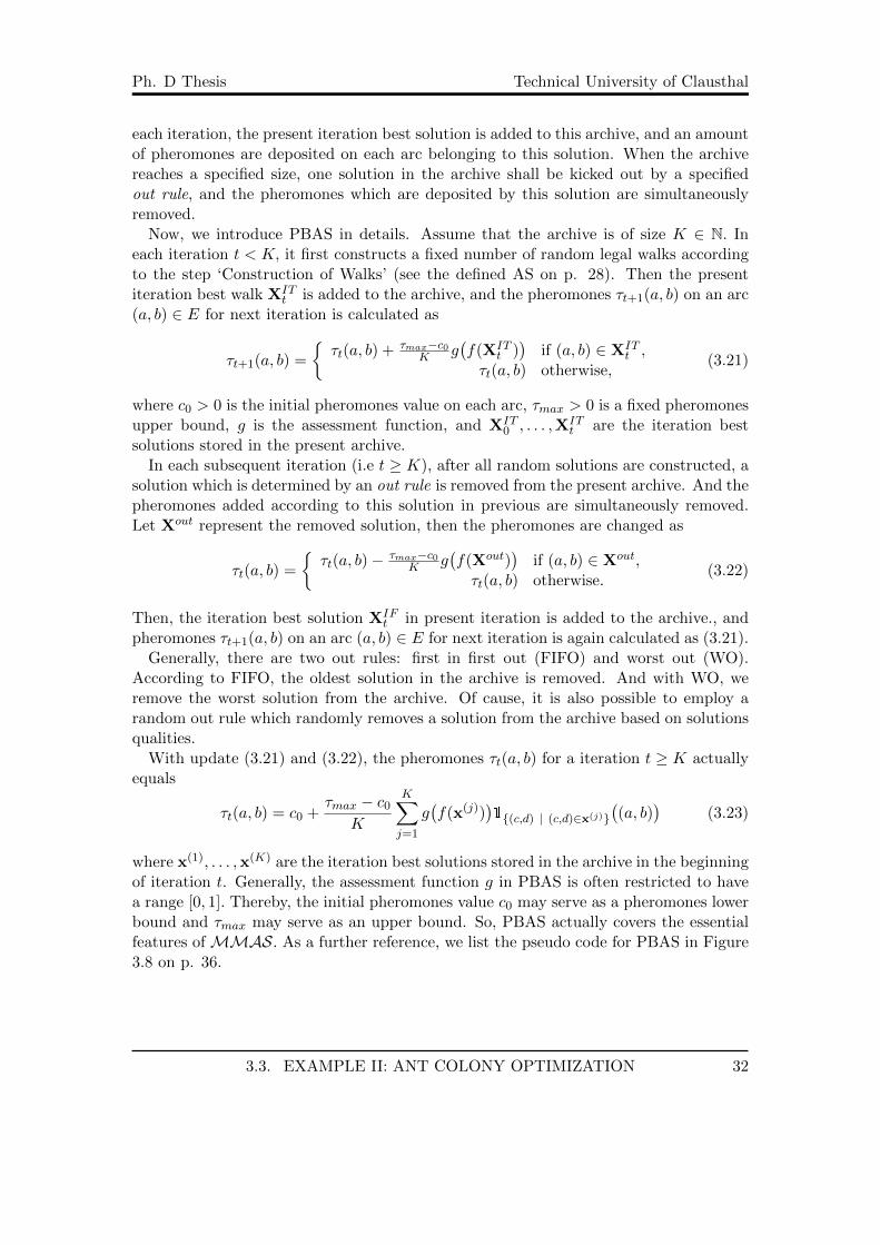
Ph. D Thesis Technical University of Clausthal
each iteration, the present iteration best solution is added to this archive, and an amountof pheromones are deposited on each arc belonging to this solution. When the archivereaches a specified size, one solution in the archive shall be kicked out by a specifiedout rule, and the pheromones which are deposited by this solution are simultaneouslyremoved.
Now, we introduce PBAS in details. Assume that the archive is of size K ∈ N. Ineach iteration t < K, it first constructs a fixed number of random legal walks accordingto the step ‘Construction of Walks’ (see the defined AS on p. 28). Then the presentiteration best walk XIT
t is added to the archive, and the pheromones τt+1(a, b) on an arc(a, b) ∈ E for next iteration is calculated as
τt+1(a, b) =
τt(a, b) + τmax−c0
K g(f(XIT
t ))
if (a, b) ∈ XITt ,
τt(a, b) otherwise,(3.21)
where c0 > 0 is the initial pheromones value on each arc, τmax > 0 is a fixed pheromonesupper bound, g is the assessment function, and XIT
0 , . . . ,XITt are the iteration best
solutions stored in the present archive.In each subsequent iteration (i.e t ≥ K), after all random solutions are constructed, a
solution which is determined by an out rule is removed from the present archive. And thepheromones added according to this solution in previous are simultaneously removed.Let Xout represent the removed solution, then the pheromones are changed as
τt(a, b) =
τt(a, b)− τmax−c0
K g(f(Xout)
)if (a, b) ∈ Xout,
τt(a, b) otherwise.(3.22)
Then, the iteration best solution XIFt in present iteration is added to the archive., and
pheromones τt+1(a, b) on an arc (a, b) ∈ E for next iteration is again calculated as (3.21).Generally, there are two out rules: first in first out (FIFO) and worst out (WO).
According to FIFO, the oldest solution in the archive is removed. And with WO, weremove the worst solution from the archive. Of cause, it is also possible to employ arandom out rule which randomly removes a solution from the archive based on solutionsqualities.
With update (3.21) and (3.22), the pheromones τt(a, b) for a iteration t ≥ K actuallyequals
τt(a, b) = c0 +τmax − c0
K
K∑j=1
g(f(x(j))
)1(c,d) | (c,d)∈x(j)
((a, b)
)(3.23)
where x(1), . . . ,x(K) are the iteration best solutions stored in the archive in the beginningof iteration t. Generally, the assessment function g in PBAS is often restricted to havea range [0, 1]. Thereby, the initial pheromones value c0 may serve as a pheromones lowerbound and τmax may serve as an upper bound. So, PBAS actually covers the essentialfeatures ofMMAS. As a further reference, we list the pseudo code for PBAS in Figure3.8 on p. 36.
3.3. EXAMPLE II: ANT COLONY OPTIMIZATION 32
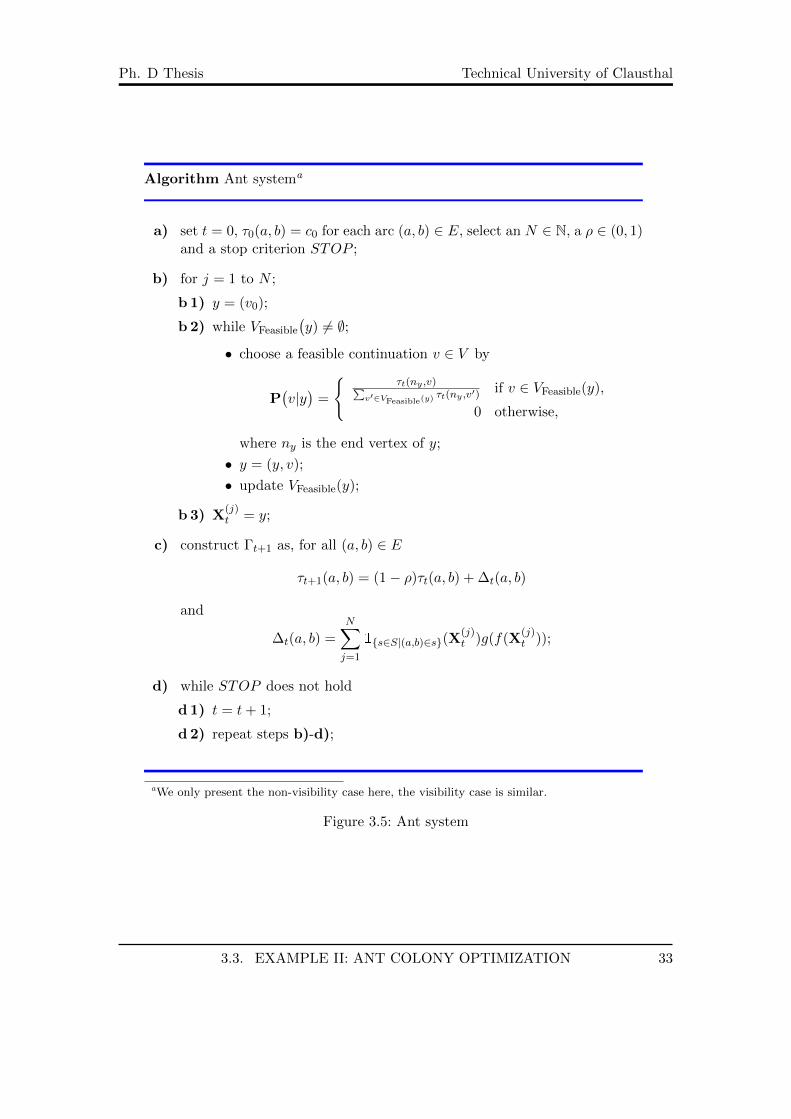
Ph. D Thesis Technical University of Clausthal
Algorithm Ant systema
a) set t = 0, τ0(a, b) = c0 for each arc (a, b) ∈ E, select an N ∈ N, a ρ ∈ (0, 1)and a stop criterion STOP ;
b) for j = 1 to N ;
b 1) y = (v0);
b 2) while VFeasible
(y) 6= ∅;
• choose a feasible continuation v ∈ V by
P(v|y)
=
τt(ny ,v)∑
v′∈VFeasible(y)τt(ny ,v′)
if v ∈ VFeasible(y),
0 otherwise,
where ny is the end vertex of y;
• y = (y, v);
• update VFeasible(y);
b 3) X(j)t = y;
c) construct Γt+1 as, for all (a, b) ∈ E
τt+1(a, b) = (1− ρ)τt(a, b) + ∆t(a, b)
and
∆t(a, b) =
N∑j=1
1s∈S|(a,b)∈s(X(j)t )g(f(X
(j)t ));
d) while STOP does not hold
d 1) t = t+ 1;
d 2) repeat steps b)-d);
aWe only present the non-visibility case here, the visibility case is similar.
Figure 3.5: Ant system
3.3. EXAMPLE II: ANT COLONY OPTIMIZATION 33

Ph. D Thesis Technical University of Clausthal
Algorithm Ant colony system
a) set t = 0, initialize Γ0 and a stop criterion STOP ;
b) for j = 1 to N ;
b 1) y = (v0);
b 2) while VFeasible(y) 6= ∅;• choose a feasible continuation v ∈ V by
v =
argmaxv∈VFeasible(y)τt(ny, v) if u ≥ q,
b if u < q,
where ny is the end vertex of y, and b is chosen as in AS;
• y = (y, v);
• update VFeasible(y);
b 3) apply the local update
τt(a, b) = (1− ρlocal)τt(a, b) + ρlocal · c1
for each arc (a, b) ∈ y;
b 4) X(j)t = y;
c) update the best solution XBFt found so far and construct Γt+1 as
τt+1(a, b) = (1− ρglobal)τt(a, b) + ρglobal∆t(a, b)
where
∆t(a, b) =
g(f(XBF
t )) if (a, b) ∈ XBFt ,
0 otherwise,
for each arc (a, b) ∈ E;
d) while STOP does not hold
d 1) t = t+ 1;
d 2) repeat steps b)-d);
Figure 3.6: Ant colony system algorithm
3.3. EXAMPLE II: ANT COLONY OPTIMIZATION 34

Ph. D Thesis Technical University of Clausthal
Algorithm MAX -MIN ant system
a) set t = 0, initialize Γ0 and select a stop criterion STOP ;
b) for j = 1 to N ;
b 1) y = (v0);
b 2) while VFeasible(y) 6= ∅;• choose a feasible continuation v ∈ V as AS;
• y = (y, v);
• update VFeasible(y);
b 3) X(j)t = y;
c) calculate XITt ,XBF
t and select Xupdt from XIT
t ,XBFt , then construct
Γt+1 with Xupdt as
τt+1(a, b) =
max
(1− ρ)τt(a, b), τmin
if (a, b) /∈ Xupd
t ,
min
(1− ρ)τt(a, b) + ρ · g(f(Xupdt )), τmax
otherwise
for each arc (a, b) in E;
d) while STOP does not hold
d 1) t = t+ 1;
d 2) repeat steps b)-d);
Figure 3.7: MAX -MIN ant system
3.3. EXAMPLE II: ANT COLONY OPTIMIZATION 35

Ph. D Thesis Technical University of Clausthal
Algorithm Population based ant system
a) set t = 0, initialize Γ0 and select a stop criterion STOP ;
b) for j = 1 to N ;
b 1) y = (v0);
b 2) while VFeasible(y) 6= ∅;• choose a feasible continuation v ∈ V as AS;
• y = (y, v);
• update VFeasible(y);
b 3) X(j)t = y;
c) pick out the iteration best solution XITt from X
(1)t , . . . ,X
(N)t ;
d) if t ≤ K, add XITt to the archive, and construct Γt+1 as
τt+1(a, b) =
τt(a, b) + τmax−c0
K g(f(XIT
t ))
if (a, b) ∈ XITt ,
τt(a, b) otherwise,
for each arc in E;
e) if t ≥ K, use the out rule to remove a solution from the archive, say Xout,and
τt(a, b) =
τt(a, b)− τmax−c0
K g(f(Xout)
)if (a, b) ∈ Xout,
τt(a, b) otherwise.
for each (a, b) ∈ E, then add XIFt into the archive and construct Γt+1 as
step d);
f) while STOP does not hold
f 1) t = t+ 1;
f 2) repeat steps b)-f);
Figure 3.8: Population based ant system
3.3. EXAMPLE II: ANT COLONY OPTIMIZATION 36
Ph. D Thesis Technical University of Clausthal
3.4 Example III: estimation of distribution algorithms
Estimation of distribution algorithms (EDA) are initially motivated for efficiently sim-ulating the robust genetic algorithm through probabilistic models, see [PGL02]. For adetailed survey on EDA, see [HP11]. Here, we concentrate only on some practical EDAwhich employ the so-called univariate marginal models, e.g. univariate marginal dis-tribution algorithm [MP96], the population based incremental learning [Bal94], and thecompact genetic algorithm [HLG99]. For some theoretical EDA which concern multivari-ate marginal models, see the literature [HGC95], [PM98], [PGCP00], [PGL02], [Pel05],[MP96], [DBIV+97] and [SG00] as a reference.
3.4.1 Feasible solutions and univariate models
It is rather popular in genetic algorithms [Mic96] that the feasible solutions of COinstances are represented as binary strings of a fixed length. As EDA are motivated forsimulating genetic algorithms, they shall follow this representation. Hence, we assumehere that the underlying feasible set S ⊆ 0, 1L for some L ∈ N. Actually, we can assumefurther that S = 0, 1L by introducing a penalty objective value for those infeasiblebinary strings as discussed in CE. Thereby, we consider here, without loss in generality,a minimizing CO instance (S, f, 0) with S = 0, 1L for some L ∈ N.
Here, we discuss only those EDA which evolve univariate marginal models. Generally,a univariate marginal model on 0, 1L is a product distribution Π =
(Π(1), . . . ,Π(L)
)on 0, 1L such that each Π(i) =
(Π(0; i),Π(1; i)
)is a Bernoulli distribution5 with
success probability Π(1; i) and failure probability Π(0; i) = 1−Π(1; i) for all i = 1, . . . , L.And by distribution Π, a random binary string s = (b1, . . . , bL) ∈ 0, 1L is then sampledwith a probability
Π(s) =L∏i=1
[Π(0; i)
]10(bi) ·
[Π(1; i)
]11(bi)
where we use a convention that 00 = 1. In details, we can generate a random string s =(b1, b2, . . . , bL) sequentially by Π with each bi generated independently by the Bernoullidistribution Π(i) for all i = 1, . . . , L. In the sequel, we shall write the family of univariatemarginal models on 0, 1L as Pum.
Extensively, a univariate marginal model is a mechanism which produces a solutionwith each of the building blocks generated independently. Here, a building block meansa component on a solution. For example, an arc is a building block of a walk; a letteris a building block of a string. Obviously, the distributions ∈ Pce serve as univariatemarginal models in CE. However, the pheromones matrices ∈ Paco do not serve asunivariate marginal models in ACO, since the selection of a continuing arc for a partiallegal walk is dependent on the end vertex of the present partial walk.
5The Bernoulli distribution is distribution of a random variable which takes value 1 with a successprobability p ∈ [0, 1] and value 0 with probability 1− p.
3.4. EXAMPLE III: ESTIMATION OF DISTRIBUTION ALGORITHMS 37

Ph. D Thesis Technical University of Clausthal
Evidently, we can simplify a univariate model Π =(Π(b; i)
)b∈0,1;i=1....,L
∈ Pum as
a vector(π1, . . . , πL
), where each πi := Π(1; i) represents the success probability in the
i-th Bernoulli distribution Π(i) for i = 1, . . . , L. Then, the corresponding probability ofgenerating a random string s = (b1, . . . , bL) ∈ 0, 1L can be written as
Π(s) =L∏i=1
[1− πi
]10(bi) · π11(bi)i .
Of cause, there are also some EDA which employs multivariate marginal models. Ex-amples are Bayesian optimization algorithm (BOA, [Pel05]), extended compact geneticalgorithm (ECGA, [SG00]), mutual-information-maximizing-input-clustering algorithm(MIMIC, [DBIV+97]), bivariate marginal distribution algorithm (BMDA, [PM98]) andfactorized distribution algorithm (FDA, [MMR99]). Generally, a multivariate marginalmodel is a model which concerns mutual interactions of building blocks on some positionsin the generation of a random solution. A typical example of multivariate models is theso-called Bayesian network, which describes the mutual dependencies of different posi-tions on a random solution through a directed graph with each node as a position andeach arc indicating a probabilistic dependency, see [PM98] for details. Although thereare some EDA which employ multivariate marginal models, they can not apply easily topractical optimization problems. The main reason here is that learning a multivariatemarginal model (from the sampled data) itself is generally rather time consuming, forexample learning a good Bayesian network for a large data may require a prohibitiverunning time. Hence, we concentrate only on those EDA with univariate marginal mod-els.
3.4.2 Simulating uniform crossover by a univariate marginal model
EDA are initially motivated for simulating genetic algorithms through probabilistic mod-els. Typically, they simulate the uniform crossover. As a reference, we now give a briefintroduction to this.
Crossover is a very important operator for a genetic algorithm [Mic96]. It takes acrucial role in the performance of a genetic algorithm. Generally, it takes in two presentsolutions (parents), and then produce two new solutions (children) hoping that the newsolutions can preserve good properties of their parents. For a reference to crossover, seeSection A.7 in the Appendix.
Uniform crossover is one of the most frequently used crossover operators in geneticalgorithms. Suppose that p(1) = (b1, . . . , bL) ∈ S and p(2) = (a1, . . . , aL) ∈ S are twoarbitrarily fixed binary strings, where recall that the underlying feasible set S is assumedto be 0, 1L. Then, uniform crossover may produce two children c(1) = (c1, . . . , cL) ∈ Sand c(2) = (d1, . . . , dL) for these two parents p(1) and p(2) by setting each
ci =
ai if pi < 0.5bi if pi ≥ 0.5
and di =
bi if ci = aiai if ci = bi
(3.24)
where pi is a random variate generated by the uniform distribution on [0, 1], for i =1, . . . , L.
3.4. EXAMPLE III: ESTIMATION OF DISTRIBUTION ALGORITHMS 38

Ph. D Thesis Technical University of Clausthal
Let πi be the frequency of bit 1 in ai, bi i.e.
πi =11(ai) + 11(bi)
2
is the relative frequency of bit 1 at position i in the two parents, for each i = 1, . . . , L.Obviously, each ci in child c(1) can only take values in 0, 1, since ai, bi ∈ 0, 1. By theuniform crossover (3.24)
P[ci =1
]= P
[ci = 1, ci = ai
]+ P
[ci = 1, ci = bi
]= P
[ai = 1, ci = ai
]+ P
[bi = 1, ci = bi
]= P
[ci = ai
∣∣ ai = 1]·P[ai = 1
]+ P
[ci = bi | bi = 1
]·P[bi = 1
].
Note that in (3.24), the random event [ci = ai] is independent of [a1 = 1] and the randomevent [ci = bi] is also independent of [bi = 1]. Thereby,
P[ci = 1
]= P
[ci = ai
]·P[ai = 1
]+ P
[ci = bi
]·P[bi = 1
]= 0.5 ·P
[ai = 1
]+ 0.5 ·P
[bi = 1
]= 0.5 ·
(P[ai = 1
]+ P
[bi = 1
]).
Since the two parents p(1), p(2) are fixed, bi, ai are also fixed. Therefore,
P[ai = 1
]= 11(ai) and P
[bi = 1
]= 11(bi).
As a result,
P[ci = 1
]=
P[ai = 1
]+ P
[bi = 1
]2
=11(ai) + 11(bi)
2= πi.
This means that each ci in child c(1) can be equivalently generated by a Bernoulli dis-tribution with success probability πi. A similar discussion applies to each position di onchild c(2), although c(2) is completely determined by c(1).
Let Πp(1),p(2) =(π1, π2, . . . , πL
). Obviously, Πp(1),p(2) ∈ Pum is a univariate marginal
model. Producing a new solution from p(1), p(2) by uniform crossover (3.24) is then equiv-alent to drawing a random solution from model Πp(1),p(2) . Therefore, we may simulateuniform crossover by sampling from this univariate marginal model.
Actually, we can further think Πp(1),p(2) as a univariate marginal model learned from
the ‘sample’ p(1), p(2). Then, uniform crossover in genetic algorithms may serve asa ‘Learning-Reproducing’ procedure i.e. we learn a model from two parents and thenreproduce two children by the learned model. The EDA discussing in this Section arejust inspired by this procedure. They may extend this procedure in several directions.
3.4. EXAMPLE III: ESTIMATION OF DISTRIBUTION ALGORITHMS 39

Ph. D Thesis Technical University of Clausthal
3.4.3 Univariate marginal distribution algorithm
Univariate marginal distribution algorithm (UMDA), [MP96], extends uniform crossover(3.24) for two parents into a Learning-Reproducing procedure for ‘multi-parents’. Itwants to simulate ‘multi-parents’ crossover by univariate marginal models.
Let P = p(1), . . . , p(n) be a population of parents, where n ≥ 1 and
p(1) =(b1,1, b2,1, . . . , bi,1. . . . , bL,1
)p(2) =
(b1,2, b2,2, . . . , bi,2. . . . , bL,2
)· · · · · ·
p(j) =(b1,j , b2,j , . . . , bi,j . . . . , bL,j
)· · · · · ·
p(n) =(b1,n, b2,n, . . . , bi,n. . . . , bL,n
)with bi,j ∈ 0, 1 for all i = 1, . . . , L and j = 1, . . . , n. In a multi-parents uniformcrossover, a child c = (c1, . . . , cL) ∈ S for these n parents can be generated as
ci = bi,ri , ri is a number randomly chosen from 1, . . . , n (3.25)
for all i = 1, . . . , L, namely each ci is a random variable uniformly distributed overbi,1, bi,2, . . . , bi,j , . . . , bi,n. Obviously, (3.25) extends the uniform crossover (3.24). Tosimulate (3.25), we can learn a univariate marginal model ΠP = (π1, . . . , πL) ∈ Pumsuch that each πi is the relative frequency of bit 1 at position i in the population P i.e.
πi =
∑nj=1 11(bi,j)
n(3.26)
for i = 1, . . . , L. Then, the child c defined in (3.25) for the parents population P isintrinsically a random solution satisfying distribution ΠP .
By (3.26), UMDA can extend the Learning-Reproducing procedure underlying theuniform crossover for two parents to a procedure involving multi-parents. Initially, itsamples a number of random solutions by the uniform distribution ∈ Pum, and collectthem in a memory. In each subsequent iteration, UMDA shall select out some promisingsolutions from the present memory as a parents population P, by a fixed choice rule.Then, a univariate marginal model ΠP ∈ Pum is learned from P by (3.26) and somechildren for P are produced by sampling from ΠP . Finally, the memory for the nextround is updated according to a memory update rule.
Formally, UMDA may take in the following as input parameters:
• a fixed memory size M ∈ N,• a fixed parents population size n ∈ N which is often determined by a fixed selection
rate α ∈ (0, 1) i.e. n = α ·M,
• a fixed number of children N ∈ N,• a fixed choice rule for selecting parents,
• a fixed memory update rule for maintaining the memory,
3.4. EXAMPLE III: ESTIMATION OF DISTRIBUTION ALGORITHMS 40

Ph. D Thesis Technical University of Clausthal
• a initial memory M0 which contains M feasible solutions.
Each iteration t ≥ 0 of the algorithm can be defined as following. Where Mt meansmemory for iteration t.
Algorithm: univariate marginal distribution algorithm
Selection: Select n parents p(1)t , . . . , p
(n)t from the present memory Mt accord-
ing to the fixed choice rule, and collect them in Pt. Where each p(j)t =(
bt1,j , . . . , btL,j
)∈Mt with bti,j ∈ 0, 1, for i = 1, . . . , L and j = 1, . . . , n.
Learning: Learn a model Πt =(πt,1, . . . , πt,L
)∈ Pum from Pt by rule (3.26), i.e.
πt,i =
∑nj=1 11
(bti,j)
n
for each i = 1, . . . , L.
Reproduction: Draw a sample (children) Xt =(X
(1)t , . . . ,X
(N)t
)of size N by model
Πt, i.e. each X(j)t =
(X
(j)t (1), . . . ,X
(j)t (L)
)∈ S = 0, 1L is sampled with a
probabilityL∏i=1
πX
(j)t (i)
t,i
[1− πt,i
]1−X(j)t (i)
for j = 1, . . . , N.
Memory Update: Build a new memory Mt+1 from children Xt and present memoryMt according to the fixed memory update rule such that the size |Mt+1| = M.
As a further reference, we also write a pseudo code for UMDA in Figure 3.9 on p. 42.The choice rule here is completely inherited from genetic algorithms. The frequently
used rules are: truncate selection and random selection. In truncate selection, we requirethe parents size n smaller than the memory size M i.e. n ≤M, and we select the n bestsolutions from memory Mt as parents population Pt. And in a random selection, eachparent in Pt shall be chosen from Mt by a distribution based on solutions qualities.
The memory update corresponds to the population update in genetic algorithms.There are two commonly used rules: λ + µ-rule and (λ, µ)-rule. In a λ + µ-rule, wetake the M best solutions in Mt and Xt as the next memory Mt+1. In (λ, µ)-rule, werandomly selection M solutions based on solutions qualities from Mt and Xt as the nextmemory Mt+1. Of cause, we may also directly use Xt as Mt+1 in the case M = N. Andwhen we use the rule Xt = Mt+1 and truncate selection for parents, then the resultedUMDA becomes a particular CE with ρ = 1.
3.4.4 Population based incremental learning
Population-based incremental learning (PBIL), see [Bal94], can be seen as a restrictedversion of UMDA or a particular version of CE. It selects only the present iteration best
3.4. EXAMPLE III: ESTIMATION OF DISTRIBUTION ALGORITHMS 41

Ph. D Thesis Technical University of Clausthal
Algorithm Univariate marginal distribution algorithm
a) set t=0, initialize memory M0 randomly and a stop criterion STOP ;
b) select a parents population Pt from the present memory by a fixed choicerule;
c) build a model Πt = (πt,1, . . . , πt,L) ∈ Pum from Pt i.e. each
πt,i =
∑s=(b1,...,bL)∈Pt bi
|Pt|
for i = 1, . . . , L;
d) draw a random sample Xt by Πt;
e) build the memory Mt+1 from Xt and Mt by a fixed memory update rule;
f) while STOP does not hold
f 1) t = t+ 1;
f 2) repeat steps b)-f);
Figure 3.9: Univariate marginal distribution algorithm
solution as parent, i.e. |Pt| = 1 and truncate selection. It directly uses the producedchildren as next memory i.e. Mt+1 = Xt. The learning is similar as CE, however anoptional feature, called model mutation, may apply to the learned model.
Initially, it uses a uniform model Π−1 = (12 , . . . ,
12) ∈ Pum to produce the first memory
M0. In each iteration t ∈ N, the iteration best solution XITt =
(XITt (1), . . . ,XIT
t (L))
would be picked out from Mt, a model Πt =(πt,1, . . . , πt,L
)∈ Pum would be constructed
in a way similar as in CE, i.e. for each i = 1, . . . , L,
πt,i = (1− ρ)πt−1,i + ρXITt (i) (3.27)
where ρ ∈ (0, 1) is a fixed learning rate, and Πt−1 = (πt−1,1, . . . , πt−1,L) ∈ Pum is themodel for time t− 1. Here, observe that an empirical model ∈ Pum learned from XIT
t coincides with XIT
t itself. After Πt is constructed, an optional model mutation mayapply. The model mutation functions similarly as the mutation in genetic algorithms,i.e. both of them may introduce some purely random disturbance into the underlyingsearch so as to help in escaping from local traps. The commonly used model mutation
3.4. EXAMPLE III: ESTIMATION OF DISTRIBUTION ALGORITHMS 42

Ph. D Thesis Technical University of Clausthal
is the so called random shift. With random shift, we mutate Πt like
πt,i =
πt,i(1− cshift) if u < rMR and v < 0.5,
πt,i(1− cshift) + cshift if u < rMR and v > 0.5,πt,i otherwise,
(3.28)
for each i = 1, . . . , L, where cshift ∈ (0, 1) is a fixed shift range, rMR ∈ (0, 1) is a fixedmutation rate, u and v are independent random variates uniformly distributed over [0, 1].Finally, a number of new solutions are sampled by Πt as the next memory Mt+1. As areference, a pseudo code of PBIL is listed in Figure 3.10 below.
Algorithm Population-based incremental learning
a) set t=0, initialize M0 by the uniform distribution Π−1 ∈ Pumand a stop criterion STOP ;
b) pick out the best solution XITt from Mt;
c) construct Πt as πt,i = (1−ρ)πt−1,i+ρXITt (i) for each i = 1, . . . , L;
d) do model mutation on Πt; %optional
e) draw a new sample Mt+1 by Πt;
f) while STOP does not hold
f 1) t = t+ 1;
f 2) repeat steps b)-f);
Figure 3.10: Population-based incremental learning
3.4.5 Compact genetic algorithm
Compact genetic algorithm (cGA), see [HLG99], is a very simple algorithm which wasclaimed to efficiently simulate PBIL. In each iteration, it investigates only two feasiblesolutions and then shifts the distribution very slightly towards the better one. More
details, in iteration t, two random solutions X(1)t and X
(2)t are sampled by a present
model Πt = (πt,1, . . . , πt,L) ∈ Pum, then it builds a Πt+1 = (πt+1,1, . . . , πt+1,L) for nextround as
πt+1,i =
πt,i if X
(1)t (i) = X
(2)t (i),
πt,i + 1n if X
(1)t (i) = 1 6= X
(2)t (i),
πt,i − 1n if X
(1)t (i) = 0 6= X
(2)t (i)
for all i = 1, . . . , L, (3.29)
3.4. EXAMPLE III: ESTIMATION OF DISTRIBUTION ALGORITHMS 43

Ph. D Thesis Technical University of Clausthal
where we assume f(X(1)t ) ≤ f(X
(2)t ), and n is a large integer fixed in advance. We list
cGA in Figure 3.11 below.
Algorithm Compact genetic algorithm
a) set t = 0, initialize Π0 and a stop criterion STOP ;
b) generate two random solutions X(1)t and X
(2)t by Πt;
c) evaluate the two solutions, and to construct Πt+1 by
πt+1,i =
πt,i if X
(1)t (i) = X
(2)t (i),
πt,i + 1n if X
(1)t (i) = 1 6= X
(2)t (i),
πt,i − 1n if X
(1)t (i) = 0 6= X
(2)t (i)
for all i = 1, . . . , L;
d) while STOP does not hold
d 1) t = t+ 1;
d 2) repeat steps b)-d);
Figure 3.11: Compact genetic algorithm
3.4. EXAMPLE III: ESTIMATION OF DISTRIBUTION ALGORITHMS 44

4 A unified model-based search framework
This Chapter serves as a foundation for the next two Chapters. We shall propose a unifiedMBS framework, and formalize its underlying stochastic process. The framework coversthe essential features of the proposed MBS algorithms in Chapter 3. It is actually anextension of the theoretical algorithms investigated in our former work [WK14b] and[WK14a].
To present a unified framework, we first need a (unified) representation for the un-derlying feasible solutions which may cover the used representations in practical MBSalgorithms. Recall that, feasible solutions are represented as fixed length strings over afinite alphabet in CE and EDA, but legal walks on a construction graph in ACO. Here,we shall again employ the former representation, i.e. we represent feasible solutions asfixed length strings over a finite alphabet in the unified framework. In the future, weshall refer to this representation as string encoding or string representation. In Section4.1, we shall show that string representation actually covers the case of constructiongraph.
We also need to specify a (unified) model family before presenting the framework.Recall that, the used models families are Pce (see CE), Paco (see ACO) and Pum (seeEDA). As we choose here the string representation, we shall correspondingly specify Πce
as the model family in the framework. In Section 4.2, we shall show that under theso-called ‘feasibility construction’, the sampling in the framework can cover samplingmethods in CE, EDA and ACO. Here, feasibility construction is a concept extending thevisibility in ACO. It can be used to efficiently sample feasible solutions, and introducemutual dependencies between different positions in a random solution.
With the string representation and model family Pce, we present the unified frame-work in Section 4.3. The framework obeys the crude MBS procedure on p. 15. Tocover essential features of practical MBS algorithms, it has four virtual rules: memoryupdate rule, subsample selection rule, learning rule and model update rule. Each rulemay have different definitions ( implementations) in different MBS algorithms. Whenwe give practical definitions to the four rules, the framework may become a practicalMBS algorithm. As a reference, the used rules in practical MBS algorithms are alsosummarized in Section 4.3.
The framework eventually results in a joint stochastic process. Section 4.4 shall for-malize the process, and reveal some basic facts related to the process. We will show theprobabilistic dependencies between its marginal processes. In the next two Chapters, wewill make a detailed mathematical inspection on the process.
45

Ph. D Thesis Technical University of Clausthal
4.1 A unified representation of feasible solutions
Now, we start this Chapter by presenting a unified representation for feasible solutions.This is a necessary pre-step for presenting a unified MBS framework, as we hope theframework can cover essential features of different MBS algorithms. It may facilitate theinspection of the revealed essential features in different algorithms.
As a convention, throughout this Chapter, we shall assume a minimizing CO instance(S, f, 0) where S is the underlying feasible set, f is the objective function and the ob-jective is to find out an optimal solution in S which minimizes f.
4.1.1 Representing feasible solutions as strings
Recall that in CE, we represent feasible solutions as fixed length strings over a finitealphabet. Here, we shall again employ this representation in the framework. Namely,we assume that
S ⊆ AL = A×A× · × A︸ ︷︷ ︸L
= (a1, . . . , aL) | ai ∈ A, for each i = 1, . . . , L,
where A is a finite set called alphabet, and L ∈ N is the fixed length of feasible solutions.In the future, we shall refer to this presentation as ‘string representation’ or ‘stringencoding’.
Note that in CE, we also assume S = AL. However, we do not continue this. Weallow S 6= AL. And we call the underlying instance constrained if S 6= AL, otherwise wecall it unconstrained.
In Subsection 3.2.1, we have seen that MaxCut instances can be unconstrained stringencoded. As further examples, we now consider other problems in Section 2.2 bellow.
Example 4.1. Assume that the underlying CO instance is a TSP instance, see Sub-section 2.2.1 in Chapter 2. And let G = (V,E) be the underlying graph. Recall thateach s ∈ S here is a walk on G which starts from a vertex, traverses all other verticesexactly once and ends in the starting vertex, i.e. a Hamiltonian circle. To represent thisinstance in the above fashion, there are generally two possible methods. The first oneis to identify the vertices V as the alphabet A and the |V | + 1 as the string length L,then each feasible solution is represented as a string of length L = |V |+ 1 over vertices(alphabet) A = V satisfying that the first position is identical with the last position,and the positions in between can not be identical with any other position. Of cause, un-der this representation, the underlying instance is constrained since S ( AL = V |V |+1.The other one is to represent feasible solutions as binary strings of length n2 wheren = |V |. We can label the vertices as 0, 1, 2, . . . , n − 1. Then, the arcs are labeled as(0, 1), (0, 2), . . . , (0, n − 1), · · · , (n − 1, 0), (n − 1, 1), . . . , (n − 1, n − 1). Given a feasibletour (solution), we can represent it as a binary string that we set bij as 0 if arc (i, j) ison the tour, otherwise we write bij = 1, for all arc (i, j). Under this case, the underly-ing CO instance is also constrained string encoded with alphabet A = 0, 1 and lengthL = n2.
4.1. A UNIFIED REPRESENTATION OF FEASIBLE SOLUTIONS 46

Ph. D Thesis Technical University of Clausthal
Example 4.2. Assume that the underlying CO instance is an AP (assignment problem)instance, see Subsection 2.2.2 in Chapter 2. Now, a feasible solution is an assignment ofn jobs to m machines where n ≤ m. Let J be the collection of jobs, andM the collectionof machines. We label the jobs ∈ J as 1, . . . , n, and machines ∈ M as 1, . . . ,m. Then,an assignment from J to M can be simply represented as a string of length L = nover alphabet A = M such that each position i on string represents the label of thecorresponding machine to which the i-th job is assigned, for i = 1, . . . , n. Of cause,under this representation, the underlying instance is constrained. And only those stringswith unrepeated alphabet are feasible.
Example 4.3. Assume that the underlying CO instance is a KP (knapsack problem)instance, see Subsection 2.2.4 in Chapter 2. A feasible solution here is a set of itemswhich are needed to be packed in a knapsack. Let K be the finite collection of all possibleitems. A feasible solution is a subset of K with total weight smaller than a specifiedcapacity of the knapsack. We label items in K as 1, . . . , |K|, and write bi = 1 if the i-thitem is packed in the knapsack and b0 = 0 if the i-th item is not packed. Then a feasiblesolution can be written as a string of length L = |K| over alphabet A = 0, 1. Underthis representation, the instance is also constrained. The feasible strings are those whichhave a ‘legal’ total weight.
In fact, string representation is very popular in mathematical optimization. For ex-ample, in linear programming (see [KV02] or Section A. 4 in the Appendix), feasiblesolutions are generally represented as strings over reals. Actually, string representationmay apply to all CO instances. Let (S′, f ′, 0) be an arbitrarily fixed CO instance. Wecan identify S′ as an alphabet. Then, each feasible solution can be seen as a string oflength 1 over the alphabet A = S′, although it may not be efficient.
For convenience, we now introduce some standard operations and terminologies ofstrings which may be frequently used in the future. We use notation to denote theempty string over A. Let x = (x1, . . . , xm) and y = (y1, . . . , yn) be two strings. Then
• |x| = m represents the length of string x, particularly | | = 0;
• we write x ⊆ y if string y extends string x, i,e, m ≤ n and
for all i = 1, . . . ,m, xi = yi,
with a convention that is extended by an arbitrary string;
• we write a ∈ x for the case that item a is in string x i.e.
there exists i = 1, . . . ,m, a = xi;
• we write (a, b) ∈ x for the case that
there exists i = 1, . . . ,m− 1, a = xi and b = xi+1;
• for any l ≤ |x| = m, we write x|l for the leading string (x1, . . . , xl) with a conventionthat x|0 = ;• let a be an item , we use (x, a) to mean the concatenation of string x with item a,
i.e. (x, a) =(x1, . . . , xn, a
).
4.1. A UNIFIED REPRESENTATION OF FEASIBLE SOLUTIONS 47

Ph. D Thesis Technical University of Clausthal
4.1.2 Relation with other frequently used representations
As a unified representation for MBS algorithms, it is necessary for us to show that thestring encoding actually covers other frequently used representations. Recall that, otherused representations in MBS algorithms are binary strings (in EDA, see Section 3.4) andconstruction graph (in ACO, see Section 3.3). Of cause, binary strings are a particularcase of the representation here. Thereby, we only need to discuss the case of constructiongraph.
Recall that in ACO, a feasible solution is represented as a legal walk on a constructiongraph which starts in a fixed vertex v0, traverses each of other vertices at most once, andends in a vertex without unvisited continuations (feasible continuations), see Subsection3.3.2. Similar with Example 4.1, we may write a legal walk as a string of verticesor arcs. However, when we represent legal walks as strings over vertices, the resultedstrings may be of different lengths since the underlying construction graph may not befully connected. Note that, whether the resulted strings here are of a same length is notessential. We can fill the end of each string with copies of a virtual vertex so as to makethem of the same length.
Let G = (V,E) be a construction graph. We now introduce a symbol 4 /∈ V ∪ E tothe graph as a virtual vertex, and denote the resulted graph as G′ = (V ∪4, E). Notethat, a legal walk on G can contain at most |V | vertices. Thereby, the lengths of theresulted strings are at most |V |. Let s = (s1, . . . , sn) be the string representation of anarbitrary legal walk on G with n ≤ |V | and each si ∈ V . Then, s can be equivalentlyextended as a string of length |V | + 1 over vertices on graph G′. Actually, we can add|V | + 1 − n (or |V | − n) many copies of the virtual vertex 4 into the end of s so as toextend it to be a string s′ of length |V |+ 1 over vertices on graph G′, i.e.
s′ = (s1, . . . , sn,4,4, . . . ,4︸ ︷︷ ︸|V |+1−n
),
and then assign the same objective value to s′.In ACO, the feasible solutions are limited to be legal walks on a graph. Of cause, it
is also possible that feasible solutions are other kinds of subgraphs. Typically, feasiblesolutions may be trees, see e.g. the minimum spanning tree problem [KV02]. Here, atree means a subgraph which is connected but contains no circuit, see also A. 1 in theAppendix. It can be uniquely determined by its arcs. Therefore, we can represent atree as a binary string by assigning value 1 to those arcs on the underlying graph whichbelong to the tree, and 0 to the arcs which do not belong to the tree. In more detail,we can first label the arcs E of the underlying graph G as 1, 2, . . . , |E|, then a tree canbe written as a string (b1, . . . , b|E|) of length |E| over 0,1 such that bi = 1 means thei-th arc is on the tree, and bi = 0 means the i-th arc is not on tree for i = 1, . . . , |E|.
4.1.3 Introducing constraints under string encoding
In the above, we have shown that string encoding applies to all CO instances, and coversother representations used in MBS algorithms. From Examples 4.1-4.3, we also see that
4.1. A UNIFIED REPRESENTATION OF FEASIBLE SOLUTIONS 48
Ph. D Thesis Technical University of Clausthal
the underlying CO instance may be constrained under this representation, i.e. S 6= ALwhere S is the underlying feasible set, A is the alphabet and L is the length of the(encoded) strings. To tell whether a string in AL is feasible in the constrained case, wecan introduce some constraints such that a string is feasible if and only if it satisfies (ormodels) all the constraints.
As an example, we assume that the underlying instance is a TSP instance, and weemploy the vertices V as the alphabet A. By Example 4.1, we can represent each feasiblesolution as a string of length |V | + 1 over A = V. Then, a string s = (s1, . . . , s|V |+1) ∈V |V |+1 is feasible if and only if it holds that:
• s1 = s|V |+1;
• for all i, j = 1, . . . , |V |, i 6= j ⇒ si 6= sj .
The above two conditions are the introduced constraints.Now, we use Ω to denote the collection of possible constraints for the underlying CO
instance under string encoding, and we set Ω = ∅ for the unconstrained case. For astring s ∈ AL, we write s |= Ω to mean that s satisfies all the introduced constraints.Here, we use a convention that s |= ∅ for every s ∈ AL. Then, the underlying feasibleset S can written as s ∈ AL | s |= Ω. And the corresponding optimization can beformulated as
mins∈ALf(s)
s.t. s |= Ω(4.1)
where ‘s.t.’ shorts for ‘subject to’. Note that, (4.1) is actually a general form for CO,since each CO instance can be string encoded.
It is very interesting that with string encoding, we can represent many CO instancesas a Linear Programming instance. For example, if we write feasible solutions in a TSPinstance as strings over vertices like in Example 4.1 and label the vertices by integers,then resulted optimization in (4.1) shall become a linear (integer) program, namely,
mins=(s1,...,s|V |+1)∈V |V |+1f(s) =
|V |∑i=1
w(si, si+1
)s.t.
i) si − sj 6= 0 for all i, j = 1, . . . , |V | with j 6= i,
ii) s1 − s|V |+1 = 0,
where we label the vertices as V = 1, . . . , |V |, and w(i, j)
is the constant weight onarc (i, j).
4.1. A UNIFIED REPRESENTATION OF FEASIBLE SOLUTIONS 49

Ph. D Thesis Technical University of Clausthal
4.2 A unified model family and feasibility construction
Recall that, MBS optimize models instead of solutions. Thereby, we still need to specifya (unified) model family before presenting the framework. Here, a necessary criterionfor choosing a model family for the framework is that the ‘sampling’ in various practicalMBS algorithms can be formulated as special cases of the sampling by a model from thespecified family. Recall that the model families used in MBS algorithms are Pce in (3.2)on p. 17, the pheromones matrices Paco in (3.15) on p. 30 and the univariate marginalmodels Pum in Subsection 3.4.1. With the string representation, we shall again employPce as the model family in the unified framework. However, here we shall not use thesampling in CE, but define another sampling mechanism called feasibility constructionwhich is an extension of the visibility in ACO. Note that the feasibility construction isnot a new idea, it has been presented in our former work [WK14b] and [WK14a]. In thisSection, we shall see that feasibility construction indeed covers those sampling methodsin CE, ACO and EDA.
4.2.1 A review to the model family PceAs formulated in Section 4.1, the underlying feasible set S ⊆ AL for some finite alphabetA and an encoded solutions length L ∈ N. Recall that, a model Π ∈ Pce is a productdistribution (
Π(1), . . . ,Π(L))
=(Π(a; i)
)a∈A;i=1,...,L
on the product space AL = A× · · · × A such that each
Π(i) =(Π(a; i)
)a∈A
is a distribution on alphabet A. By Π ∈ Pce, a random string s = (a1, . . . , aL) in AL isgenerated with each position ai chosen independently by Π(i) for i = 1, . . . , L, i.e. it ischosen with a probability
Π(s) =L∏i=1
Π(ai; i).
In the unified framework, we shall employ Pce as the specified model family. But we donot directly generate random solutions by models in Pce. On the one hand, this mayproduce infeasible strings (here, S 6= AL may hold), although we have discussed in CEthat we can remove the constraints by introducing a penalty objective value. On theother hand, the above random solution generating mechanism can not cover the samplingin ACO. To cover the sampling in ACO, we shall use the sampling mechanism proposedin our former works [WK14b] and [WK14a]. We shall call the mechanism as feasibilityconstruction. To show a difference in the sampling with CE, we shall employ the symbolP to represent the model family Pce in the future.
4.2. A UNIFIED MODEL FAMILY AND FEASIBILITY CONSTRUCTION 50

Ph. D Thesis Technical University of Clausthal
4.2.2 A unified sampling mechanism: feasible construction
To propose the feasibility construction, we need some auxiliary definitions. We say thata string y ∈ A≤L = ∪A∪A2 ∪ · · · ∪AL is a feasible partial solution if there exists afeasible solution s ∈ S ⊆ AL with y ⊆ s (i.e. s extends y). For each i = 0, . . . , L, we useRi to denote the collection of all feasible partial solutions of length i. Obviously, R0 isjust the singleton where recall that is the empty string. And for each i = 1, . . . , L,the collection Ri can be formally defined as
Ri =
(y, a)∣∣y ∈ Ri−1, a ∈ A and ∃s ∈ S with (y, a) ⊆ s
(4.2)
where recall that (y, a) indicates the concatenation of partial solution y with item a. Ofcause, S = RL ⊆ AL, and R :=
⋃Li=0Ri ⊆ A≤L is the collection of all possible partial
solutions.For each i = 0, . . . , L − 1, we call a function Ci(·; ·) : Ri × A 7→ [0, 1] which satisfies
that for each y ∈ Ri• Ci(y; ·) is a distribution on A, i.e.
∑a∈ACi(y; a) = 1,
• for each a ∈ A, if (y, a) /∈ Ri+1, then Ci(y; a) = 0,
as a feasibility distribution for position i+ 1. If Ci(·; ·) is a feasibility distribution, we letCi(y) := a ∈ A|Ci(y; a) > 0 denote the support of Ci(y; ·). Obviously, support Ci(y)only contains feasible continuations of y, and Ci(y; ·) is a distribution concentrating onthose feasible continuations Ci(y).
Note that, for any CO instance we can define a sequence of feasibility distributionsCi(·; ·)L−1
i=0 . For example, we may define a sequence of feasible distributions as
Ci(y; a) :=
1|a∈A|(y,a)∈Ri+1| for each a ∈ A with (y, a) ∈ Ri+1,
0 otherwise.(4.3)
for i = 0, . . . , L− 1 and y ∈ Ri. In the future, we shall refer to (4.3) as the ‘non-greedyfeasibility distributions’.
We may also introduce some greedy insight into the feasibility distributions. As anexample, we consider a TSP instance with weight function w and n vertices in V . Andwe assume here that feasible solutions (Hamiltonian circles) are represented as stringsover vertices. Then, each Ri contains strings with exactly i different vertices. For eachi = 0, . . . , L− 1 and y = (v1, . . . , vi) ∈ Ri, we can define a feasibility distribution as
Ci(y; v) :=
[w(vi,v)]−β
∑(y,v)∈Ri+1
[w(vi,v)]−β if (y, v) ∈ Ri+1,
0 otherwise,
where β > 0 is a fixed constant, v ∈ V is an arbitrary vertex. Then, the support Ci(y)shall collect the vertices which have not occurred in y yet. And the vertices ∈ Ci(y)which introduce smaller traveling weights from the end of y (i.e. vi) would be morepreferred as a continuation of y.
4.2. A UNIFIED MODEL FAMILY AND FEASIBILITY CONSTRUCTION 51

Ph. D Thesis Technical University of Clausthal
Now, we are ready to introduce the feasibility construction method. Feasibility con-struction is a method inspired by the visibility concept for ACO, see (3.14). It producesa random solution stepwise by a mixture of a production distribution in P (i.e. Pce)and the feasibility distributions. Let Π ∈ P be a product distribution on AL, andCi(·; ·)L−1
i=0 a constructed sequence of feasibility distributions. Starting with the emptystring , a partial solution y is then extended by a feasible continuation a ∈ Ci(y) witha selection probability defined as
Q(a; y, i+ 1,Π) :=Π(a; i+ 1)Ci(y; a)∑
a′∈Ci(y) Π(a′; i+ 1)Ci(y; a′), (4.4)
where a convention 00 = 0 is employed. With (4.4), the selection probability of a complete
solution s = (s1, . . . , sL) ∈ S would be
Q((s1, . . . , sL); Π
):=
L−1∏i=0
Q(si+1; s|i, i+ 1,Π
), (4.5)
where recall that s|i = (s1, . . . , si) and s|0 = . Obviously, the support of (4.5) is a subsetof S. In other word, by (4.5), we will always produce feasible solutions. As a summary,a pseudo random solution generation algorithm with feasibility construction is listed inFigure 4.1 below.
Algorithm Random solution generation by feasibility construction
a) set y = , and i = 0;
b) for i < L do;
b 1) select an item from A with probability
Q(a; y, i+ 1,Π) :=Π(a; i+ 1)Ci(y; a)∑
a′∈Ci(y) Π(a′; i+ 1)Ci(y; a′).
b 2) y = (y, a);
b 3) i = i+ 1;
c) output y;
Figure 4.1: Random solution generation by feasibility construction
Note that, feasibility construction also covers the unconstrained case where S = AL.
4.2. A UNIFIED MODEL FAMILY AND FEASIBILITY CONSTRUCTION 52

Ph. D Thesis Technical University of Clausthal
In this case, we can set
Ci(y; a) =1
|A| for each i = 0, . . . , L− 1 and y ∈ Ri. (4.6)
Then the Q(a; y, i+ 1,Π) defined in (4.4) is degenerated to Π(a; i+ 1). Obviously, thiswill result in a sampling as in CE and EDA. Note also that, in non-greedy feasibilityconstruction (see (4.3)), we take Ci(y; ·) as the uniform distribution on set a ∈ A|(y, a) ∈Ri+1, and then
Q(a; i+ 1, y,Π) = Q′(a; i+ 1, y,Π) :=
Π(a;i+1)∑
a′∈A,(y,a′)∈Ri+1Π(a′;i+1) if (y, a) ∈ Ri+1
0 otherwise.(4.7)
4.2.3 Cover the sampling of ACO
Recall that, in ACO, feasible solutions are represented as legal walks on a constructiongraph, i.e. those walks starting from a unique vertex, traversing other vertices at mostonce until no feasible continuations available. Here, we assume a construction graphG = (V,E) with V = v0, v1, . . . , vK, v0 is the unique starting vertex for all legal walks.A legal walk on G can be represented as a string over vertices V, or a string over arcsE, and these two representations are equivalent. More details, let
v0, (v0, a1), a1, (a1, a2), . . . , (an−1, an), an
be a legal walk on G, it can be equivalently represented as a string (v0, a1, . . . , an) oververtices and a string
((v0, a1), (a1, a2), . . . , (an−1, an)
)over arcs E. Due to equivalence
of these three representations, we may use them interchangeably. We will see that theessential samplings in ACO can be formulated as a particular case of the feasibilityconstruction if we write legal walks as strings over arcs.
In ACO, we generate a legal walk by iteratively extending a partial legal with a feasiblecontinuation. Here, a partial legal walk is a walk starting from the unique starting vertexv0, and traversing other vertices at most once. Let y = (v0, a1, . . . , am) be a partial legalwalk (here, we write walks as strings over vertices). We use VFeasible(y) to denote thecollection of all feasible continuations to y. Then
VFeasible(y) =a ∈ V | (am, a) ∈ E, a /∈ v0, a1, . . . , am
.
When VFeasible(y) = ∅, y is a (complete) legal walk. Assume VFeasible(y) 6= ∅, Γ =(τ(c, d)
)c,d∈V is the present pheromones matrix. Then, an ant may select a feasible
continuation a ∈ VFeasible(y) to y by the choice probability
P[a | y
]=
τ(am,a)∑
v′∈VFeasible(y)τ(am,v′)
if a ∈ VFeasible(y),
0 otherwise.(4.8)
4.2. A UNIFIED MODEL FAMILY AND FEASIBILITY CONSTRUCTION 53
Ph. D Thesis Technical University of Clausthal
Moreover, if there is a visibility information η(y; ·) available, the choice probability maybecome
P[a | y
]=
[τ(am,a)
]α[η(y;a)
]β∑v′∈VFeasible(y)
[τ(am,v′)
]α[η(y;v′)
]β if a ∈ VFeasible(y),
0 otherwise,
(4.9)
where η(y; v) is typically some greedy information like the distance information e.g.η(y; v) = 1/d(am, v) in TSP, and α, β > 0 are constants. In application, α is typicallychosen to be 1.0, see [DS04], [DMC96], [DG97a], [DG97b], [SH00] etc. Therefore, (4.9)is generally
P[a | y
]=
τ(am,a)
[η(y;a)
]β∑v′∈VFeasible(y)
τ(am,v′)[η(y;v′)
]β if a ∈ VFeasible(y),
0 otherwise,
(4.10)
in practice.To show that the feasibility construction covers (4.8) and (4.10), we represent legal
walks as equal-length strings over arcs. We use E ∪ 4 as the underlying alphabet A,where 4 is a symbol not in E. We fill the end of each legal walk with copies of 4 soas to make them of length L = |V | − 1. Note that, each legal walk on the constructiongraph G can contain at most |V | − 1 arcs. According to the pheromones matrix, we candefine a product distribution
Π =(Π(a, b); i
)(a,b)∈A;i=1,...,L
=(Π(a, b); i
)(a,b)∈E∪4;i=1,...,|V |−1
as, for i = 1, . . . , L = |V | − 1, and (a, b) ∈ A = E ∪ 4,
Π((a, b); i
)=
p·τ(a,b)∑
(c,d)∈E τ(c,d) if (a, b) ∈ E,1− p if (a, b) = 4,
(4.11)
where p ∈ (0, 1) is an arbitrarily fixed constant. Obviously, Π((a, b); 1
)= · · · =
Π((a, b);L
)for each item (arc) (a, b) ∈ A. Each Π
(·; i)
indicates a selection in A =E ∪ 4 for the i-th position on a random string.
Corresponding to the non-visibility choice probability (4.8), we can construct non-greedy feasibility distributions Ci(·; ·)i=0,...,L−1 as following
• for each arc (a, b) ∈ A = E ∪ 4, C0
(; (a, b)
)= 0 if a 6= v0, and
C0
(; (a, b)
)=
1
|b ∈ V | (v0, b) ∈ E|if a = v0,
• for each legal partial walk Y =((v0, a1), . . . , (am−1, am)
)(here, we represent walks
as strings over arcs), let
EFeasible(Y ) =
(a, b) ∈ E ∪ 4 | a = am, b ∈ V, b /∈ v0, a1, . . . , am,
4.2. A UNIFIED MODEL FAMILY AND FEASIBILITY CONSTRUCTION 54

Ph. D Thesis Technical University of Clausthal
and we define, for all (a, b) ∈ A = E ∪ 4,
Cm(Y ; (a, b)
)=
1 if EFeasible(Y ) = ∅, (a, b) = 4,0 if EFeasible(Y ) = ∅, (a, b) 6= 4,
1|EFeasible(Y )| if EFeasible(Y ) 6= ∅, (a, b) ∈ EFeasible(Y ),
0 otherwise.
(4.12)
Then, by the non-greedy feasibility construction (4.7), the probability for choosing anarc (a, b) ∈ A as the continuation to a legal partial walk Y =
((v0, a1), . . . , (am−1, am)
)is
Q((a, b);Y,m+ 1,Π
)=
Π((a, b);m+ 1
)Cm(Y ; (a, b)
)∑(c,d)∈AΠ
((c, d);m+ 1
)Cm(Y ; (c, d)
) ,where we again use the convention 0
0 = 1. In the case that VFeasible(y) 6= ∅, EFeasible(Y )is also non empty and equals (am, b) | b ∈ VFeasible(y), where y = (v0, a1, . . . , am) isthe vertices representation of Y. According to the third and fourth cases in (4.12), theprobability
Q((am, a);Y,m+ 1,Π
)=
Π((am, a);m+ 1
)Cm(Y ; (am, a)
)∑c∈VFeasible(y) Π
((am, c);m+ 1
)Cm(Y ; (am, c)
)=
Π((am, a);m+ 1
)1
|EFeasible(Y )|∑c∈VFeasible(y) Π
((am, c);m+ 1
)1
|EFeasible(Y )|
=Π((am, a);m+ 1
)∑c∈VFeasible(y) Π
((am, c);m+ 1
) ,for a vertex a ∈ VFeasibility(y). By the first case in (4.11), we have
Q((am, a);Y,m+ 1,Π
)=
p·τ(am,a)∑(h,d)∈E τ(h,d)∑
c∈VFeasible(y)p·τ(am,c)∑
(h,d)∈E τ(h,d)
=τ(am, a)∑
c∈VFeasible(y) τ(am, c),
which is exactly the same as the first case in the choice probability (4.8) for non-visibility. When a /∈ VFeasibility(y), we can similarly show that the probability is 0.And if VFeasibility(y) = ∅ i.e. y is a complete legal walk, then EFeasibility(Y ) is also empty.In this case, the probability for choosing 4 is 1 provided that Y contains less than Larcs. So, we deterministically add copies of 4 to the end of a ‘complete’ Y until itcontains L arcs.
For covering the visibility case (4.10), we only need to redefine C0
(; (v0, a)
)as[
η((v0); a)]β∑
c∈VFeasibility(y)
[η((v0); c)
]β
4.2. A UNIFIED MODEL FAMILY AND FEASIBILITY CONSTRUCTION 55
Ph. D Thesis Technical University of Clausthal
where (v0) means the string only consisting of v0, and the feasibility distributions (4.12)as
Cm(Y ; (a, b)
)=
1 if EFeasible(Y ) = ∅, (a, b) = 4,0 if EFeasible(Y ) = ∅, (a, b) 6= 4,[
η(y;b)]β
∑c∈VFeasibility(y)
[η(y;c)
]β if EFeasible(Y ) 6= ∅, (a, b) ∈ EFeasible(Y ),
0 otherwise,
where Y =((v0, a1), . . . , (am−1, am)
), y = (v0, v1, . . . , vm) is its vertices representation.
The verification is similar as in the case of non-visibility.
4.2.4 Probabilistic dependencies in the sampling
In the above discussion, we have seen that feasibility construction covers the samplingsused in CE, ACO and EDA. Therefore, by feasibility construction, it is ‘legal’ to useP = Pce as the model family in the unified framework. Actually, feasibility constructionmay also introduce some ‘crude’ probabilistic dependencies into the sampling.
Recall that, if we generate a random solution s = (a1, . . . , aL) only by a model Π =(Π(a; i)
)a∈A;i=1,...,L
∈ P, then positions on s are generated independently i.e.
P[ai∣∣ (a1, . . . , ai−1)
]= P
[ai]
= Π(ai; i)
for each i = 1, . . . , L, where we use a convention that (a1, a0) = . In feasibility con-struction, the next item may depend on the finished leading string, i.e.
P[ai∣∣ (a1, . . . , ai−1)
]= Q
(ai; (a1, . . . , ai−1), i,Π
)6= P[ai]
in the constrained case.Actually, feasibility construction can be made more extensive so as to cover some
linkage learning mechanism [PM98] into the sampling. However, we will not discuss thisissue here, we leave it as a future work.
4.2. A UNIFIED MODEL FAMILY AND FEASIBILITY CONSTRUCTION 56
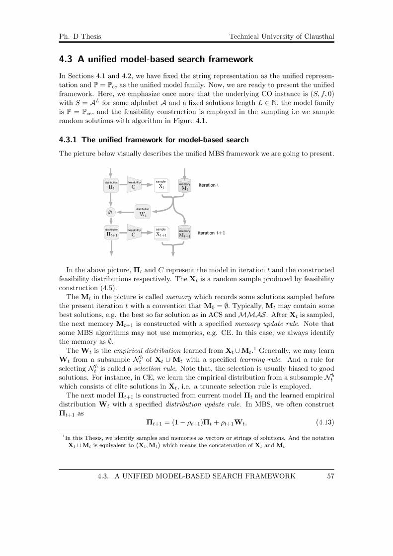
Ph. D Thesis Technical University of Clausthal
4.3 A unified model-based search framework
In Sections 4.1 and 4.2, we have fixed the string representation as the unified represen-tation and P = Pce as the unified model family. Now, we are ready to present the unifiedframework. Here, we emphasize once more that the underlying CO instance is (S, f, 0)with S = AL for some alphabet A and a fixed solutions length L ∈ N, the model familyis P = Pce, and the feasibility construction is employed in the sampling i.e we samplerandom solutions with algorithm in Figure 4.1.
4.3.1 The unified framework for model-based search
The picture below visually describes the unified MBS framework we are going to present.
distribution
sample
distribution
distributionmemory
feasibility
memorysamplefeasibility
iteration
iteration
In the above picture, Πt and C represent the model in iteration t and the constructedfeasibility distributions respectively. The Xt is a random sample produced by feasibilityconstruction (4.5).
The Mt in the picture is called memory which records some solutions sampled beforethe present iteration t with a convention that M0 = ∅. Typically, Mt may contain somebest solutions, e.g. the best so far solution as in ACS andMMAS. After Xt is sampled,the next memory Mt+1 is constructed with a specified memory update rule. Note thatsome MBS algorithms may not use memories, e.g. CE. In this case, we always identifythe memory as ∅.
The Wt is the empirical distribution learned from Xt ∪Mt.1 Generally, we may learn
Wt from a subsample N bt of Xt ∪Mt with a specified learning rule. And a rule for
selecting N bt is called a selection rule. Note that, the selection is usually biased to good
solutions. For instance, in CE, we learn the empirical distribution from a subsample N bt
which consists of elite solutions in Xt, i.e. a truncate selection rule is employed.The next model Πt+1 is constructed from current model Πt and the learned empirical
distribution Wt with a specified distribution update rule. In MBS, we often constructΠt+1 as
Πt+1 = (1− ρt+1)Πt + ρt+1Wt, (4.13)
1In this Thesis, we identify samples and memories as vectors or strings of solutions. And the notationXt ∪Mt is equivalent to
(Xt,Mt
)which means the concatenation of Xt and Mt.
4.3. A UNIFIED MODEL-BASED SEARCH FRAMEWORK 57

Ph. D Thesis Technical University of Clausthal
where ρt+1 is a learning rate. Obviously, learning rates correspond to the smoothparameters in CE and the evaporation rates in ACO. In the sequel, we shall concentrateon this kind of update, and we shall refer to (4.13) as the ‘basic recursion’. In update(4.13), the learning rate ρt+1 reflects the relative importance of the empirical distributionWt.
Now, we list the unified framework for MBS algorithms in Figure 4.2 below. Obviously,this framework covers the essential features of CE, ACO and EDAs. Note that, thisframework itself is an optimization algorithm with four components, namely memoryupdate rule, selection rule, learning rule and possibly the distribution update rule. Later,we shall summarize the used rules in the practical MBS algorithms. The mathematicalstudy in Chapters 5 and 6 shall be based on this framework.
Algorithm A unified model-based search framework
Elements:an instance (S, f) with S ⊆ AL for some finite set A and L ∈ N, asample size N ∈ N, a sequence of learning rates (ρt)t≥1 on (0, 1], an initialdistribution Π0 ∈ P, a sequence of feasibility distributions Ci(·; ·) fori = 0, . . . , L − 1, a memory update rule, a subsample selection rule, alearning rule, and a stop criterion STOP.
algorithm:
a) set M0 = ∅ and t = 0;
b) do while STOP does not hold;
b 1) draw a sample Xt using algorithm in Figure 4.1 on p. 52 withΠ = Πt and Ci(·; ·)’s;
b 2) construct Mt+1 from Mt and Xt with the memory update rule;
b 3) select a subsampleN bt from Mt∪Xt with the subsample selection
rule;
b 4) learn a distribution Wt ∈ P from N bt with the learning rule;
b 5) Πt+1 = (1− ρt+1)Πt + ρt+1Wt;
Figure 4.2: A unified model-based search framework for combinatorial optimization
4.3. A UNIFIED MODEL-BASED SEARCH FRAMEWORK 58

Ph. D Thesis Technical University of Clausthal
4.3.2 A summary of commonly-used rules in practical model-based searchalgorithms
From Sections 4.1 and 4.2, we see that the sampling method in the framework coversthe sampling methods in practical MBS algorithms. For covering the essential featuresof those practical algorithms, we now summarize the commonly used rules for the fourcomponents from the practical MBS algorithms in Chapter 3.
Memory update rules
Memory update rule tells which solutions should be stored for a possible use in nextround. By a memory update rule, we can construct the next memory Mt+1 from thepresent memory Mt and sample Xt. Usually, this rule may affect the empirical distri-bution in next round, because Wt is learning from Mt ∪Xt. In general, there are threekinds of memory update rules. Here, we call them non memory (NM), globally truncatememory update (GTMU) and locally truncate memory update (LTMU) respectively.
In NM, Mt ≡ ∅ for all t ∈ N, i.e we do not store the feasible solutions seen previ-ously. Typical examples of MBS algorithms with NM, are the basic CE (cross entropyalgorithm, see [Rub99]), CE/tdsp (cross entropy algorithm with time-dependent smoothparameters, see [CJK07]), CE/as (ant-like cross entropy algorithm, see [WK14b]), AS(ant system, see [DMC96]), cGA (compact genetic algorithm, see [HLG99]), UMDA(univariate marginal distribution algorithm, see [PM98]), and PBIL (population-basedincremental learning, see [Bal94]).
In GTMU, the next memory Mt+1 consists of some best solutions in Mt and Xt. Indetails, we order solutions in Mt ∪Xt as
f(s(n1)) ≤ f(s(n2)) ≤ . . . ≤ f(s(nM+N ))
where N is the size of Xt and M is the size of Mt, and then set
Mt+1 = (s(n1), . . . , s(nM )). (4.14)
MBS algorithms with GTMU are e.g. ACS (ant colony system, see [DG97b]), GBAS(graph-based ant system, see [Gut00]), and GBCE (graph-based cross entropy algorithm,see [Mar05]) and UMDA.
In LTMU, a fixed out rule is employed to remove a number of solutions from Mt, thenMt+1 shall consist of the same number of best solutions in Xt as well as the remainingsolutions in Mt. In details, let O = (x(1), . . . , x(k)) ⊆Mt be k solutions determined byan out rule, and I = (y(1), . . . , y(k)) the k best solutions in Xt. Then
Mt+1 =[Mt −O
]∪ I.2 (4.15)
Note that, we may keep the out rule disabled in the first several iterations until thememory has reached a specified size. Typical examples of out rules are worst out (WO)and first in first out (FIFO). In WO, we kick out a fix amount of worst solutions. InFIFO, we kick out a number of oldest solutions. A type example of LTMU is PBAS(population-based ant system [GM02]).
2Here Mt −O is the string which is formed by removing O from Mt.
4.3. A UNIFIED MODEL-BASED SEARCH FRAMEWORK 59

Ph. D Thesis Technical University of Clausthal
4.3.3 Selection rules
In MBS, the empirical distribution Wt is typically learned from a subsample N bt of
Xt ∪Mt. A selection rule may tell how to select N bt in each iteration t. This rule may
directly affect the empirical model Wt. In practice, selection rules can be collectedas identity selection (ID), memory identical selection (MID), truncate selection (TS),random selection (RS) and memory random selection (MRS).
In ID selection, we set N bt = Mt ∪Xt. MBS algorithms with ID selection are e.g. AS
(ant system, see [DMC96]) and cGA (compact genetic algorithm, see [HLG99]).In MID selection, we set N b
t = Mt+1. Note that, Mt+1 is also a subsample of Mt∪Xt.Typical algorithms with MID selection are e.g. ACS (ant colony system, [DG97b]),PBAS (population-based ant system, [GM02]), GBAS (graph-based ant system, [Gut00])and GBCE (graph-based cross entropy, [Mar05]).
TS selection is completely similar with the GTMU memory update. It collects afixed number of best solutions in Mt ∪Xt as N b
t . MBS algorithms with TS selection aree.g. CE (cross entropy algorithm, [RK04]), CE/tdsp (cross entropy with time-dependentsmooth parameters, see [CJK07]), CE/as (ant-like cross entropy algorithm, [WK14b]),UMDA (univariate marginal distribution algorithm, [MP96]) and PBIL (population-baseincremental learning, [Bal94]).
In the case of RS, we select N bt from Xt∪Mt by probabilities proportional to qualities
of solutions, i.e.
P[s ∈ N b
t
∣∣ s ∈Mt ∪Xt
]=
g(f(s))∑s′∈Mt∪Xt
g(f(s′))for all s ∈Mt ∪Xt, (4.16)
where g(·) is a fixed positive non-increasing function. Examples of RS selection can befound in UMDA and some other EDAs (see Hauschild et al[HP11]).
MRS selection is similar with RS selection. However, here N bt is sampled from Mt+1
i.e.
P[s ∈ N b
t
∣∣ s ∈Mt ∪Xt
]=
g(f(s))∑s′∈Mt+1
g(f(s′))for all s ∈Mt+1, (4.17)
where g(·) is a fixed positive non-increasing function. Algorithm with MRS is e,g,MMAS [SH00]
4.3.4 The learning rules
Given N bt , an empirical model Wt ∈ P = Pce shall be learned by a learning rule. In
MBS algorithms, popular learning rules are uniform learning (UL) and weighted learning(WL).
Typical examples of UL may be CE [Rub99], UMDA [MP96] and PBIL [Bal94]. WithUL, we see the solutions in N b
t equivalently, and use the relative frequencies as theempirical distribution Wt, i.e.
Wt(a; i) :=
∑s∈N bt
1a(si)
|N bt |
for all a ∈ A and i = 1, . . . , L. (4.18)
4.3. A UNIFIED MODEL-BASED SEARCH FRAMEWORK 60

Ph. D Thesis Technical University of Clausthal
By WL, we see the solutions inequivalently, and use the weighted frequencies as Wt.Let g(·) be a positive real function satisfying g(s(1)) ≥ g(s(2)) ⇐⇒ f(s(1)) ≤ f(s(2)).Then, we may calculate the empirical distribution as
Wt(a; i) :=
∑s∈N bt
1a(si)g(s)∑s∈N bt
g(s)for all a ∈ A and i = 1, . . . , L. (4.19)
Algorithms with WL are various kinds of ACO algorithms (see [DS04]).Of cause, we may make the learning phase more flexible, i.e.
Wt(a; i) :=
∑s∈N bt
1a(si)g(s, t)∑s∈N bt
g(s, t)for all a ∈ A and i = 1, . . . , L, (4.20)
for some fixed positive function g with g(s(1), t) ≥ g(s(2), t) ⇐⇒ f(s(1)) ≤ f(s(2))for t ∈ N. We shall refer to this kind of learning as time dependent weighted learning(TDWL) in the sequel.
4.3.5 Distribution update rules
With the present model Πt and the empirical model Wt, we can construct the modelΠt+1 for next round according to a fixed distribution update rule. MBS algorithmsgenerally employ the basic recursion (4.13) to form next model. According to the rangeof (ρt)t≥1, we can collect MBS into two classes, namely, conservative and radical.
Conservative distribution update is popular in MBS. It restricts each learning rate in(0, 1). For examples, see CE [RK04], ACO [DS04] and EDAs using univariate marginaldistributions [HP11] except for UMDA (univariate marginal distribution algorithm,[PM98]).
Radical distribution update occurs only in the UMDA [PM98]. It directly uses theempirical distribution Wt as the next model Mt+1, in other word ρt ≡ 1.
Actually, we can make the update of distributions in the framework more extensivelyby formulating it as a (possibly random) function U : P× P 7→ P. And if a definition ofU is given, we can set the next model Πt+1 as U(Πt,Wt). In MBS, the basic recursion(4.13) is the most popular definition for U . Of cause, we can employ other definitions.For example, in PBIL (population-based incremental learning), we can define the U asa composition of the basic recursion and the additional model mutation function.
Although we can make the update of models more extensive, we will still stick to(4.13) in the future, because of its popularity.
As a summary to this Section, Table 4.1 on p. 62 shows the used rules in practicalMBS algorithms.
4.3. A UNIFIED MODEL-BASED SEARCH FRAMEWORK 61

Ph. D Thesis Technical University of Clausthal
Table 4.1: The four rules for some practical MBS algorithms
algorithms memory update selection rule learning rule distr. update
CE [Rub99] NM TS UL ρt ≡ ρ ∈ (0, 1)CE/as [WK14b] NM TS UL ρt ∈ (0, 1)GBCE [Mar05] GTMU MID UL ρt ∈ (0, 1)
CE/tdsp [CJK07] NM TS UL ρt ∈ (0, 1)AS NM ID WL ρt ≡ ρ = 1
ACS GTMU MID WL ρt ≡ ρ ∈ (0, 1)MMAS LTMU (WO) MRS WL ρt ≡ ρ ∈ (0, 1)
PBAS [GM02] LTMU (FIFO) MID WL ρt ≡ ρ = 1GBAS [Gut00] GTMU MID WL ρt ≡ ρ ∈ (0, 1)1-ANT [NW06] GTMU ID WL ρt ≡ ρ ∈ (0, 1)ASelite[BHS97] GTMU ID WL ρt ≡ ρ ∈ (0, 1)ASrank[BHS97] GTMU ID WL ρt ≡ ρ ∈ (0, 1)
ASbw[CdVHM00] GTMU ID WL ρt ≡ ρ ∈ (0, 1)UMDA NM or GTMU TS or RS UL ρt ≡ ρ = 1PBIL NM TS UL ρt ≡ ρ ∈ (0, 1)cGA NM ID UL ρt ≡ ρ ∈ (0, 1)
EDAs [ZM04] NM TS or RS UL ρt ≡ ρ = 1
4.3. A UNIFIED MODEL-BASED SEARCH FRAMEWORK 62

Ph. D Thesis Technical University of Clausthal
4.4 The underlying stochastic process
In Section 4.3, we have presented the unified framework for MBS algorithms based onthe string representation. The framework specifies P = Pce as model family, and employsthe feasibility construction in sampling. It iteratively evolves models in P according tofour rules i.e. a memory update rule, a selection rule, a learning rule and a distributionupdate rule. Due to this evolution, it eventually results in a joint stochastic process. Asan end to this Chapter, this Section shall formally define the process.
4.4.1 Input parameters and strategy
The framework generally takes the following as input parameters (see also Figure 4.2):
• a fixed initial model Π0 ∈ P;
• a fixed feasibility distributions sequence Ci(·; ·)L−1i=0 ;
• a fixed learning rates sequence (ρt)t=1,2,... with each ρt ∈ (0, 1];
• a fixed sample size N ∈ N;
• a fixed memory size M ∈ N;
• a fixed subsample size Nb ∈ N;
• a fixed memory update rule M;
• a fixed subsample selection rule S;
• a fixed learning rule L.Note that, we restrict the memory update rule to be the basic recursion
Πt+1 = (1− ρt+1)Πt + ρt+1Wt.
Note also that, the learning rate ρt is required to be positive. The main reason is thatpractical MBS algorithms generally employ positive learning rates, see Table 4.1.
A strategy of the framework is then a combination of a fixed feasibility distributionssequence, a fixed learning rates sequence, a fixed memory update rule, a fixed subsampleselection rule and a fixed learning rule. With a specified strategy, the framework maycorrespond to a particular MBS algorithm. For example, if we use the unconstrainedfeasibility distributions (4.6), fix a constant learning rate ρt ≡ ρ > 0, and employ resp.,rules NM (non memory), TS (truncate selection) and UL (uniform learning) for memoryupdate, subsample selection and learning, the framework then becomes a CE algorithm(see Table 4.1). In the sequel, we use notation “M =” to short for the words “memoryupdate rule is”, similarly for the notation “S =” and “L =”. As an example, “M =NM”, “S = TS” and “L = UL” correspond resp., to the sentences “memory update ruleis non-memory”, “subsample selection rule is truncate selection” and “learning rule isuniform learning”.
4.4.2 The underlying stochastic process
With a fixed strategy, the framework will iteratively evolve models ∈ P = Pce. Thiswould result in a joint stochastic process (see A. 4 in the Appendix for a definition of
4.4. THE UNDERLYING STOCHASTIC PROCESS 63

Ph. D Thesis Technical University of Clausthal
stochastic process) (Πt; Xt; Mt;N b
t ; Wt
)t=0,1,2,...
.
Where Πt ∈ P represents the model in iteration t which is a product distribution on theproduct space AL = A×· · ·×A; Xt ∈ SN is a random sample drawn by a mixture of Πt
and the feasibility distributions CiL−1i=0 with probabilities defined in (4.5); Mt ∈ SM
is the memory maintained by a fixed rule M, which records some ‘best’ solutions seenin times 0, 1, 2, . . . , t − 1; N b
t ∈ SNb is a subsample of Xt ∪Mt selected by a fixed ruleS; Wt ∈ P is an ‘empirical’ distribution learned from N b
t by a fixed rule L. Initially, astarting model ∈ P is determined i.e. Π0 is fixed, and the memory is set to be an emptyvector i.e. M0 = ∅. Then, the process iteratively evolves models as in Figure 4.3 below.The thin dashed (gray) line indicates the subsample selection in the case that S = MID
Πt Xtsampling
Mt
time t− 1 Ntselect S
select S
Wtlearn L Πt+1
(1− ρt+1)
ρt+1
Mt+1 time t+ 1
S = MID, MRS
update M
update M
Figure 4.3: Underlying process
or MRS (memory identity selection or memory random selection), and the thin (gray)line for other cases.
In the above Figure, Πt = (Πt(1), . . . ,Πt(L)) is the model for iteration t, where each
Πt(i) =(Πt(a; i)
)a∈A
describes a distribution on the fixed alphabet A i.e.
∑a∈A
Π(a; i) = 1 and Π(a; i) ≥ 0 for each a ∈ A
for i = 1, . . . , L. The state space P = Pce of the marginal process(Πt
)t=0,1,2,
is contin-
uous, since the state space P(A) of the process(Πt(i)
)t=0,1,2,...
is continuous for eachi = 1, . . . , L.
By the feasibility construction (4.5), we can draw a random sample
Xt =(X
(1)t , . . . ,X
(N)t
)where each
X(l)t =
(X
(l)t (1), . . . ,X
(l)t (L)
)∈ S ⊆ AL
4.4. THE UNDERLYING STOCHASTIC PROCESS 64

Ph. D Thesis Technical University of Clausthal
for l = 1, . . . , N, by Πt and feasibility distributions. In details, for each l = 1, . . . , N
and each i = 0, . . . , L− 1, X(l)t (i+ 1) is sampled by a conditional probability
Q(X
(l)t (i+1); X
(l)t (1, . . . , i), i+1,Πt
)=
Πt
(X
(l)t (i+ 1); i+ 1
)Ci(Xt(1, . . . , i); X
(l)t (i+ 1)
)∑a∈Ci
(X
(l)t (1,...,i)
)Πt
(a; i+ 1
)Ci(Xt(1, . . . , i); a
)where X
(l)t (1, . . . , i) = X
(l)t |i =
(X
(l)t (1), . . . ,X
(l)t (i)
)is the leading partial solution up to
length i in X(l)t , and we use the convention that X
(l)t |0 = . Therefore, for each x ∈ SN ,
P[Xt = x
∣∣ Πt,Ht−1
]= P
[Xt = x
∣∣ Πt
],
for each t ≥ 0, where Ht−1 is the history of the joint process up to time t− 1 i.e.
Ht−1 =Π0,X0,M0,N b
0 ,W0; · · · ; Πt−1,Xt−1,Mt−1,N bt−1,Wt−1
,
and we use a convention thatH−1 = ∅. Obviously, the state space AL of marginal process(Xt
)t=0,1,2...
is SN which is finite.
The state space of the marginal process(Mt
)t=0,1,2,...
is SM ∪∅ which is also finite.
Initially, M0 = ∅. Then, the memory Mt ∈ SM is a vector containing M solutions foreach iteration t ≥ 1. In each iteration t ∈ N, the memory shall be updated by the fixedmemory rule M. By the rule, the next memory Mt+1 is then a subsample of Xt ∪Mt.For example, if M = GTMU (global truncate memory update rule), we shall take thebest M solutions in present sample Xt and present memory Mt as the next memoryMt+1. Obviously, for each m ∈ SM ,
P[Mt+1 = m
∣∣ Xt,Πt,Mt,N bt ,Wt,Ht−1
]= P
[Mt+1 = m
∣∣ Xt,Mt
],
for each t ∈ N.The marginal process
(N bt
)t=0,1,2,...
also has a finite state space i.e. SNb . Each N bt is
a subsample of Xt ∪Mt chosen by the fixed selection rule S. When S = MID (memoryidentity selection) or S = MRS (memory random selection), it is a subsample of nextmemory Mt+1, thereby depends the next memory Mt+1, see thin dashed (gray) line inFigure 4.3. But when S = TS (truncate selection), RS (random selection) or ID (identityselection), it is a direct subsample of Xt ∪Mt, therefore does not depend on Mt+1, seethin (gray) line in Figure 4.3. Consequently, for each n ∈ SNb ,
P[N bt = n
∣∣ Xt,Πt,Mt,Mt+1,Ht−1
]= P
[N bt = n
∣∣ Xt,Mt
]holds for cases S = ID, TS, or RS, but does not hold for cases S = MID or MRS.
Similar to(Πt
)t=0,1,2,...
, the state space of marginal process(Wt
)t=0,1,2,...
is also the
continuous space P = Pce. In each iteration t ∈ N, after the subsample N bt is selected,
we shall learn an empirical model Wt from N bt by the fixed learning rule L. Like Πt,
each Wt = (Wt(1), . . . ,Wt(L)) with Wt(i) =(Wt(a; i)
)a∈A
. When L = UL (uniform
4.4. THE UNDERLYING STOCHASTIC PROCESS 65

Ph. D Thesis Technical University of Clausthal
learning), each Wt(a; i) is set to be the relative frequency of item a at the i-th positionof the subsample N b
t , see (4.18). And when L = WL (weighted learning), Wt(a; i) willbe the weighted frequency of item a at the i-th position of N b
t , see (4.19). Obviously,N bt dominates Wt, and for each w ∈ P,
P[Wt = w
∣∣ Xt,Πt,Mt,N bt ,Ht−1
]= P
[Wt = w
∣∣ N bt
],
for each t ∈ N.After Wt is learned, the next model Πt+1 is set to be a convex combination of the
present mode Πt and Wt as in the basic recursion (4.13). In details,
Πt+1(a; i) = (1− ρt+1)Πt(a; i) + ρt+1Wt(a; i) (4.21)
for all i = 1, . . . , L and a ∈ A. Hence, for each p ∈ P,
P[Πt+1 = p
∣∣ Xt,Πt,Mt,N bt ,Wt,Ht−1
]= P
[Πt+1 = p
∣∣ Πt,Wt
]=
1 if (4.21) holds,0 otherwise,
for t ∈ N.The joint process actually forms a Markov chain. By the above discussion, it is not
difficult to see that
P[(
Πt; Xt; Mt;N bt ; Wt
)= (p; x; m; n; w)
∣∣∣ Ht−1
](4.22)
= P[(
Πt; Xt; Mt;N bt ; Wt
)= (p; x; m; n; w)
∣∣∣ (Πt−1; Mt−1
)],
for p ∈ P, x ∈ SN , m ∈ SM , n ∈ SNb and w ∈ P are constants. In the future, we shallrefer to (4.22) as ‘Markov property’.
In the next two Chapters, we shall give a more detailed analysis on the joint process.We will see that the basic recursion (4.21), Markov property (4.22), memory update ruleM and subsample selection rule S take pivotal roles in the analysis.
4.4. THE UNDERLYING STOCHASTIC PROCESS 66

5 Analysis of model-based search I:reachability and a crude runtime analysis
In Chapter 4, we proposed a unified framework for MBS algorithms, see Figure 4.2.The framework covers the essential features of these MBS algorithms used in practice,i.e. each MBS algorithm may correspond to the framework equipped with a particularstrategy where a strategy for the framework is a combination of a sequence of feasibilitydistributions, a memory update rule, a subsample selection rule, a learning rule andpossibly a distribution update rule. With a fixed strategy, the framework finally resultsin a joint Markov chain
(Πt; Xt; Mt;N b
t ; Wt
)t=0,1,2,...
, see Section 4.4. From now on, weshall concentrate on this Markov chain. We will show a detailed mathematical analysisfor its asymptotic properties. The results shall carry over to these algorithms which arecovered in the framework.
We will focus on four issues in the analysis: conditions for guaranteeing to reach anoptimal solution in finitely many iterations (finite reachability); conditions for reachingan optimal solution in a polynomial runtime (runtime analysis); convergence propertyof marginal process
(Xt
)t=0,1,2,...
(absorption of solutions); and convergence property of
marginal process(Πt
)t=0,1,2,...
(absorption of models). However, in the present Chapter,we will concentrate only on finite reachability and runtime analysis. The absorption ofsolutions and models will be inspected in Chapter 6.
Conditions guaranteeing to find an optimal solution in finitely many iterations are ofgreat interests in the theoretical analysis of an optimization algorithm. For some partic-ular MBS algorithms, there are some conditions available in the literature. In [Gut00]and [Gut03], W. J. Gutjahr inspected the conditions on a particular ACO algorithmcalled GBAS (graph-based ant system). The algorithm learns the empirical distributiononly with the best solution found so far, and uses a constant learning rate ρt ≡ ρ ∈ (0, 1).In [Gut00], W. J. Gutjahr showed that when |S∗| = 1 i.e. there is a unique optimal so-lution, the probability for GBAS to reach an optimal solution in finitely many iterationsapproaches 1 as the sample size N →∞ or the constant learning rate ρ→ 0. In [Gut03],he extended the result proposed in [Gut00] by removing the restriction |S∗| = 1, i.e. heshowed that his result in [Gut00] still holds even when |S∗| > 1. In [CJK07], A. Costa etal inspected the conditions for a generalized cross entropy algorithm on unconstrainedproblems, i.e. CE/tdsp (cross entropy algorithm equipped with a sequence of smoothparameters ρtt∈N). They found conditions which imply CE/tdsp reach an optimalsolution in finitely many iterations with probability 1. In [WK14b], we extended theconditions in [CJK07] to a more general CE i.e. CE/as (ant-like CE, our frameworkwithout memory). In Section 5.3, we continue [Gut00], [Gut03], [CJK07] and [WK14b].We show that those conditions in the literature still hold in the unified framework, see
67

Ph. D Thesis Technical University of Clausthal
Theorem 5.7. The Theorem does not assume a particular algorithm, and does not im-pose a particular structure of the underlying CO instances. Therefore, it should apply toall MBS algorithms which are covered in the framework and to arbitrary CO instance.In particular, it shows that in the case of ρt ≡ ρ > 0 for a constant ρ, we may never seean optimal solution. Of cause, here we avoid the trivial case that S = S∗.
Note that ρt ≡ ρ > 0 is a common setting in practice, see Table 4.1. To show moreinsight into this case, two runtime results will be proposed in Section 5.4. Recently,runtime analysis of heuristic algorithms becomes a very popular research field, see e.g.[NW06], [DNSW07], [DJ07], [NW09], [Gut07], [Gut08], [CTCY10] and [WK14b]. Inruntime analysis, we consider conditions which make the algorithm reach an optimalsolution efficiently (i.e. in a polynomial runtime) with a large probability. Here, theruntime is a rudimentary copy of the computation complexity [AB09] in theoreticalcomputer science. Due to the famous No Free Lunch Theorem [WM97], we need toassume a particular test problem in such an analysis. In [NW06], [DNSW07], [DJ07]and [NW09], the authors proposed some runtime results for a so-called 1-ANT ACOalgorithm (a simpleMMAS with sample size N = 1 and update models only when newimprovement occurs) on some simple test problems e.g. OneMax and LeadingOne. In[Gut07], W. J. Gutjahr summarized the commonly used techniques in runtime analysis.In [Gut08], W. J. Gutjahr proposed a polynomially expected runtime forMMAS on theOneMax problem. In [CTCY10], Chen et al showed a polynomial runtime for a UMDA(univariate marginal distribution algorithm with truncate selection) on the LeadingOneproblem. In [WK14b], we showed a polynomial runtime for CE on the LeadingOneproblem. Note that the UDMA inspected in [CTCY10] is actually a particular CE witha constant smooth parameter ρ = 1. The runtime result in [WK14b] therefore extendsthe result in [CTCY10]. Note also that both 1-ANT and MMAS employ restrictedmodels and anew models only by best solution found so far. However, CE does not userestricted models, and update models by present solutions (elite solutions). Thereby, ourformer result actually complements the results in [NW06], [DNSW07], [DJ07], [NW09]and [Gut08]. In Section 5.3, we shall collect our former runtime result in Theorem 5.8.To further understand the role of subsample selection in efficiently finding an optimalsolution, we propose a new runtime result in Theorem 5.9.
The whole Chapter is arranged as: Section 5.1 formally defines the finite reachabilityand runtime, and collects some necessary assumptions which are generally fulfilled inpractice; Section 5.2 collects some helpful properties of the underlying process; Section5.3 concentrates on finite reachability; Section 5.4 concentrates the runtime analysis.
68
Ph. D Thesis Technical University of Clausthal
5.1 Definitions and assumptions
Recall that in the framework the underlying CO instance (S, f, 0) is string encoded, i.e.S ⊆ AL for a finite alphabet A and a constant L ∈ N. The model family is specified tobe P = Pce, for a definition see (3.2) on p. 17.
5.1.1 Definitions
Let τ ∈ N be a random variable denoting the first hitting time (iteration) for an optimalsolution i.e.
τ := mint ∈ N | Xt ∩ S∗ 6= ∅ ∪ ∞
(5.1)
where S∗ is the collection of optimal solutions. Then if P[τ < ∞
]= 1, we say that
(almost surely) finite reachability holds. Obviously, finite reachability concerns the ef-fectiveness of the framework. Therefore, conditions which make finite reachability holdin the framework should be of great importance. Section 5.3 shall show conditions whichmake finite reachability hold in the framework. The conditions do not impose any restric-tions on the underlying CO instance, thereby apply to all combinatorial optimizationproblems.
In the literature, see e.g. [NW06], [DNSW07], [DJ07], [NW09], [Gut07], [Gut08],[CTCY10] and [WK14b], runtime of an algorithm is generally defined as the total numberof feasible solutions evaluated before reaching an optimal solution. Note that this isa rudimentary copy of the computational complexity [AB09]. In the framework, theruntime is obviously N · τ . To express the efficiency of an algorithm, runtime is oftenformulated as a function in problem size. In the string encoding, the problem size canbe described by the encoded solutions length. Formally, we say that an algorithm has apolynomial runtime with degree n ∈ N on a problem1 P if for each instance (S′, f ′, 0) ∈ Pwith the encoded solutions length L(S′,f ′,0) ≥ Lthreshold ∈ N, the runtime of the algorithm
is bounded above by a polynomial function c ·(L(S′,f ′,0)
)n, where Lthreshold and c ∈ R+
are constants. By the standard notation in complexity, we can denote this polynomialruntime as
O((L(S′,f ′,0)
)n)where L(S′,f ′,0) is solution length of an arbitrary instance in problem P.2 Algorithmswith polynomial runtime are considered as efficient, and with low degree polynomialare practically preferred. Comparatively, an algorithm is inefficient on a problem P ifthe runtime is exponential i.e. for each (S′, f ′, 0) ∈ P the runtime is asymptoticallybounded below by an exponential function cL(S′,f ′,0) for some constant c > 1. In runtimeanalysis, we inspect conditions which imply (low degree) polynomial runtime with a highprobability. Section 5.4 will present conditions which imply a polynomial runtime on thetwo testing problem i.e. OneMax and LeadingOne, with an overwhelming probability.
1Recall that a problem is a class of instance.2See A. 5 in the Appendix for the big O notation and other notations used in runtime analysis.
5.1. DEFINITIONS AND ASSUMPTIONS 69

Ph. D Thesis Technical University of Clausthal
5.1.2 General assumptions
In the sequel, we assume that the starting model Π0 satisfies that any item from A hasa positive probability at any position i :
Π0(a; i) > 0 for all a ∈ A, i = 1, . . . , L. (5.2)
Note that in practice, Π0 is generally taken as a uniform distribution over AL whichmeets the assumption (5.2).
Without loss in generality, we may also assume that there are at least two solutions
s = (s1, . . . , sL), s′ = (s′1, . . . , s′L) with s1 6= s′1. (5.3)
Otherwise, all solutions would start with the same symbol, which could then be droppedfrom the encoding of the solutions.
Note that for a feasible solution s = (s1, . . . , sL) ∈ S, the sampling probability (4.5)
Q(s; Π
)=
L−1∏i=0
Q(si+1; s|i, i+ 1,Π
)with each
Q(si+1; s|i, i+ 1,Π) =Π(si+1; i+ 1)Ci(s|i; si+1)∑a′∈Ci(s|i) Π(a′; i+ 1)Ci(s|i; a′)
,
may be zero even in the case of an uniform Π ∈ P, where recall that s|i = (s1, . . . , si)and s|0 = . Therefore, the random solution generation algorithm in Figure 4.1 may runa risk that an optimal solution can not be sampled under any model Π ∈ P. To savethis, we assume that the constructed feasibility distributions CiL−1
i=0 are compatible tothe optimal solutions, i.e.
L−1∏i=0
Ci(s∗|i; s
∗(i+ 1))> 0 for all s∗ ∈ S∗. (5.4)
And to avoid trivial cases, we assume further that
S 6= S∗ and
L−1∏i=0
Ci(s|i; s(i+ 1)
)> 0 for some s ∈ S − S∗. (5.5)
Otherwise, the sampling would always produce optimal solutions.Note that in MBS algorithms, we often need to compare objective values of two dif-
ferent solutions. But, it may occur that two different solutions have the same objectivevalue. To deal with this embarrassing situation, we assume that
for each iteration t ∈ N if f(X(n)t ) = f(X
(m)t ) and n > m (5.6)
then we think X(n)t is better than X
(m)t , and
for each pair of iterations t ∈ N and t′ ∈ N if f(X(m)t ) = f(X
(n)t′ ) and t < t′ (5.7)
5.1. DEFINITIONS AND ASSUMPTIONS 70

Ph. D Thesis Technical University of Clausthal
then we think X(n)t′ is better than X
(m)t . Note that assumptions (5.6) and (5.7) actually
assign the time order to solutions of the same objective value i.e. we think that newsolutions are better than old solutions if they have the same objective values. Theassumptions will be employed only when we need to sort solutions in a collection.
Finally, we give assumptions on the empirical distribution Wt learned by rule L. Weassume that:
i) for all a ∈ A, i ∈ 1, . . . , L, t ∈ N,
∀s = (s1, . . . , sL) ∈ N bt si 6= a ⇒ Wt(a; i) = 0, (5.8)
∀s = (s1, . . . , sL) ∈ N bt si = a ⇒ Wt(a; i) = 1; (5.9)
ii) there exists a constants α ∈ (0, 1) such that for all a ∈ A, i ∈ 1, . . . , L, t ∈N,
Wt(a; i) > 0 ⇒ Wt(a; i) > α, (5.10)
Wt(a; i) < 1 ⇒ Wt(a; i) < 1− α. (5.11)
Note that these assumptions are fulfilled in the practically used learning rules. Recallthat practically used learning rules are of two types, namely UL (uniform learning, see(4.18) on p. 60) and WL (weighted learning, see (4.19)). In UL, Wt(a; i) is the relativefrequency of letter a at position i in the selected subsample N b
t i.e.
Wt(a; i) :=
∑s∈N bt
1a(si)
|N bt |
for all a ∈ A and i = 1, . . . , L.
Obviously, (5.8) and (5.9) are fulfilled in this case. In WL, each solution in N bt is
allocated a positive weight according to its cost value. And then Wt(a; i) calculates theweighted relative frequency of a at position i in N b
t i.e.
Wt(a; i) :=
∑s∈N bt
1a(si)g(s)∑s∈N bt
g(s)for all a ∈ A and i = 1, . . . , L,
where g is a positive weight function. Also (5.8) and (5.9) are fulfilled. Both UL andWL are time-independent learning, i.e. Wt1 = Wt2 if N b
t1 = N bt2 , for all t1 ∈ N, t2 ∈ N.
Since the state space of(N bt
)t∈N is SNb and |SNb | <∞, so
α′ := minWt(a; i) > 0
∣∣ a ∈ A, i = 1, . . . , L, t ∈ N> 0,
β′ := maxWt(a; i) < 1
∣∣ a ∈ A, i = 1, . . . , L, t ∈ N< 1.
Then obviously α := minα′, 1− β′ fulfills (5.10) and (5.11).For time-dependent learning (4.20), assumptions (5.8) and (5.9) generally still holds,
but (5.10) and (5.11) may not hold. However, most of the statements in Chapter 5 andChapter 6 will still hold, if the allocated learning weights in time-dependent learningare not changed too dramatically as iteration varies. To simplify the discussion, we willstick to the case of uniform learning or weighted learning in the sequel.
5.1. DEFINITIONS AND ASSUMPTIONS 71

Ph. D Thesis Technical University of Clausthal
5.2 Some basic properties
As a start of the analysis, we now collect some useful properties about the models(Πt)t∈N and sampling probabilities (see (4.5) on p. 52), which will be frequently usedin the present Chapter and Chapter 6.
5.2.1 On basic recursion
Recall that basic recursion (4.21)
Πt+1 = (1− ρt+1)Πt + ρt+1Wt
is the employed distribution update rule in the framework, where Πt ∈ P = Pce is thepresent model, Wt ∈ P = Pce is the model learned from a selected subsample N b
t ,ρt+1 > 0 is the learning rate for time t + 1, and Πt+1 ∈ P = Pce is the model fornext round, for t = 0, 1, 2, . . . . To facilitate our analysis, we now collect some usefulstatements closely related to this basic recursion in the following Lemma. Here, we usea convention that empty product equals 1, i.e.
∏tm=t+1 · · · = 1.
Lemma 5.1. Let 0 < rt < 1 for t = 1, 2, . . ..
a)∞∑t=1
rt =∞ ⇐⇒∞∏t=1
(1− rt) = 0 ⇐⇒∞∏t=1
(1− crt) = 0 for any 0 < c < 1.
b)t∑
m=1
rm
t∏i=m+1
(1− ri) = 1−t∏
m=1
(1− rm) for any t ≥ 1.
c) For a given sequence wt ∈ [0, 1], t = 0, 1, . . . and q0 ∈ (0, 1), the recursion
qt+1 = (1− rt+1)qt + rt+1wt, t ≥ 0, (5.12)
has the unique solution
qt = q0
t∏m=1
(1− rm) +t∑
m=1
rmwm−1
t∏i=m+1
(1− ri) (5.13)
with
0 < q0
t∏m=1
(1− rm) ≤ qt ≤ 1− (1− q0)t∏
m=1
(1− rm) < 1, t ≥ 0. (5.14)
If, in particular, wm ≡ w ∈ [0, 1] for m = 0, . . . , t− 1 then
qt = w − (w − q0) ·t∏
m=1
(1− rm). (5.15)
5.2. SOME BASIC PROPERTIES 72
Ph. D Thesis Technical University of Clausthal
And furthermore if we allow some rt = 1, then b), (5.13) and (5.15) still hold, and (5.14)becomes
0 ≤ q0
t∏m=1
(1− rm) ≤ qt ≤ 1− (1− q0)t∏
m=1
(1− rm) ≤ 1, t ≥ 0.
Proof. (see also [WK14b] and [WK14a])a) The first part is a standard result of infinite products, see e.g. [Kno90], the secondfollows as
∞∑i=0
ri =∞ ⇐⇒∞∑i=0
cri =∞.
b) Note that ri = 1− (1− ri). Then
t∑m=1
rm
t∏i=m+1
(1− ri) =t∑
m=1
[1− (1− rm)
] t∏i=m+1
(1− ri)
=t∑
m=1
t∏i=m+1
(1− ri)−t∑
m=1
t∏i=m
(1− ri)
= 1 +t−1∑m=1
t∏i=m+1
(1− ri)−t∑
m=2
t∏i=m
(1− ri)−t∏
m=1
(1− rm)
= 1−t∏
m=1
(1− rm).
c) (5.13) can be proven using induction on t. (5.15) follows from (5.13) using b). Then(5.14) follows immediately from the facts that
0 ≤t∑
m=1
rmwm−1
t∏i=m+1
(1− ri) ≤t∑
m=1
rm
t∏i=m+1
(1− ri) = 1−t∏
m=1
(1− rm).
Applying Lemma 5.1 c) to the basic recursion (4.21), we immediately get that
Lemma 5.2. If the learning rate ρt ∈ (0, 1] for each t = 1, 2, . . . , then the following holdfor all t, k ≥ 0, a ∈ A and i = 1, . . . , L :
a) Πt(a; i)∏km=1(1− ρt+m) ≤ Πt+k(a; i) ≤ 1−
(1−Πt(a; i)
)∏km=1(1− ρt+m);
b) Wt(a; i) = · · · = Wt+k−1(a; i) = 0 ⇒ Πt+k(a; i) = Πt(a; i)∏km=1(1− ρt+m), and
if we assume further that ρt ∈ (0, 1) for all t ∈ N, then the inverse implication alsoholds;
5.2. SOME BASIC PROPERTIES 73

Ph. D Thesis Technical University of Clausthal
c) for all m = 0, . . . , k − 1
Wt+m(a; i) ≡ 1 ⇒ Πt+k(a; i) = 1−(1−Πt(a; i)
) k∏m=1
(1− ρt+m),
and if we assume further that ρt ∈ (0, 1) for all t ∈ N, then the inverse implicationalso holds;
d) if ρm ∈ (0, 1) for all m ≤ t, 0 < Πt(a; i) < 1;
e) if∏∞t=1(1− ρt) = 0 and limt→∞Wt(a; i) = w, then limt→∞Πt(a; i) = w.
Proof. Statements a)-d) follows immediately from c) of Lemma 5.1 with observation tothe assumption (5.2). Now, we prove statement e).
Assume that∏∞t=1(1−ρt) = 0 and Wt(a; i)→ w as t→∞. Let ε > 0 be an arbitrarily
fixed constant. Then there exists an T ∈ N such that
w + ε ≥Wt(a; i) ≥ w − ε for all t ≥ T.
Then by (5.13) and b) of Lemma 5.1, we have that
(w + ε)−((w+ε)− 1
) t∏m=T+1
(1− ρm) ≥
(w + ε)−((w + ε)−ΠT (a; i)
) t∏m=T+1
(1− ρm) ≥
Πt(a; i) ≥ (w − ε)−((w − ε)−ΠT (a; i)
) t∏m=T+1
(1− ρm)
≥ (w − ε)− (w − ε)t∏
m=T+1
(1− ρm)
for all t ≥ T + 1. Since∏∞m=1(1 − ρm) = 0,
∏∞m=T+1(1 − ρm) = 0 for any fixed T ∈ N.
Consequently, we have
w + ε ≥ lim supt→∞
Πt(a; i) ≥ lim inft→∞
Πt(a; i) ≥ w − ε.
Note that ε is arbitrarily fixed, this results in
w = lim supt→∞
Πt(a; i) = lim inft→∞
Πt(a; i) = limt→∞
Πt(a; i).
Lemma 5.2 e) actually means that the limiting behavior of the models is dominatedby the limiting behavior of the learned empirical distributions. Hence, in the sequel
5.2. SOME BASIC PROPERTIES 74

Ph. D Thesis Technical University of Clausthal
when we want to derive a limit of the models, we often derive a limit for the empiricaldistributions in advance.
For a constructed feasibility distributions CiL−1i=0 and a feasible solution s = (s1, . . . , sL) ∈
S, we say that s is compatible to or feasible under CiL−1i=0 if and only if
L−1∏i=0
Ci(s|i; si+1
)> 0.
As a result of Lemma 5.2 d), we have immediately that
Lemma 5.3. Let CiL−1i=0 be the feasibility distributions and ρt ∈ (0, 1) for all t ∈ N,
then for any s ∈ S which is compatible to CiL−1i=0 , the probability Q(s; Πt) > 0 for all
t ≥ 0 where Q is defined in (4.5), i.e.
Q(s; Πt) =L−1∏i=0
Q(si+1; s|i, i+ 1,Πt
)and
Q(si+1; s|i, i+ 1,Πt
)=
Ci(s|i; si+1)Πt(si+1; i+ 1)∑a∈Ci(s|i)Ci(s|i; a)Πt(a; i+ 1)
. (5.16)
In particular, for each s∗ ∈ S∗, Q(s∗; Πt) > 0 for all t ≥ 0.
Note that a feasible solution can be sampled only if it is compatible to the constructedfeasibility distributions. Due to this fact, in the sequel when we refer to feasible solutions,we mean those which are feasible under (compatible to) the feasibility distributions.Note also that with assumption (5.4), optimal solutions are always feasible under thefeasibility distributions. Hence, Lemma 5.3 shows that in each iteration optimal solutionscan always have a positive chance to be sampled provided ρt ∈ (0, 1) for all t ∈ N. Butin the case ρt = 1 for some t ∈ N, this is not guaranteed.
5.2.2 A surrogate probability of Q(·; y, i,Π) and its properties
To theoretically study the framework, we need to study the letter selection probabilityQ(·; y, i,Π) (defined in (4.4), see also (5.16)) more closely.
For the unconstrained non-greedy feasibility construction (see (4.6)), Q(a; y, i,Π) =Π(a; i) holds for all a ∈ A, Π ∈ P and i = 1, . . . , L. Therefore, in this case Lemma (5.1)c) directly applies to Q(a; y, i,Πt) for all a ∈ A, y ∈ Ri−1, t ≥ 0 and i = 1, . . . , L. Ingeneral, this is not possible as Q(a; y, i,Πt) does not fulfill the recursion (5.12). Butwe can find a surrogate probability Q′(a; y, i,Πt) for Q(a; y, i,Πt), for which a similarrecursion holds under certain conditions.
The surrogate probability Q′(a; y, i,Πt) using here is also the one defined in (4.7), i.e.the selection probability for non-greedy feasibility construction. For a feasible partialsolution y ∈ Ri−1, a letter a ∈ A, a position i = 1, . . . , L, and a model Π ∈ P, we set
Q′(a; y, i,Π) :=1Ci−1(y)(a)Π(a; i)∑b∈A 1Ci−1(y)(b)Π(b; i)
(5.17)
5.2. SOME BASIC PROPERTIES 75

Ph. D Thesis Technical University of Clausthal
where we again use the convention that 00 = 0. Obviously, for an unconstrained non-
greedy feasibility construction, we have Q(a; y, i,Π) = Q′(a; y, i,Π) = Π(a; i), and for anon-greedy feasibility construction, we have Q(a; y, i,Π) = Q′(a; y, i,Π).
In general, although Q(a; y, i,Π) 6= Q′(a; y, i,Π), we can employ this surrogate proba-bility to boundQ. To do this, we need bounds for the constructed feasibility distributions.Let
η := max Ci(y; a)|y ∈ Ri, a ∈ A, i = 0, 1, 2, . . . , L− 1 (5.18)
andλ := min Ci(y; a) > 0|y ∈ Ri, a ∈ A, i = 0, 1, 2, . . . , L− 1 . (5.19)
Obviously, 1 ≥ η ≥ λ > 0. Now, we define two bounding functions ~(x) and `(x) forx ∈ [0, 1] as
~(x) :=ηx
λ+ (η − λ)xand `(x) :=
λx
η − (η − λ)x. (5.20)
The following Lemma collects some properties of these two bounding functions.
Lemma 5.4. a) `(x) ≤ x ≤ ~(x), ~(x) = 1− `(1− x) and `(x) = 1− ~(1− x).
b) ~ and ` are both continuous and strictly increasing with `(0) = ~(0) = 0, `(1) =~(1) = 1.
c) Suppose xnn∈N is a convergent sequence in [0, 1] then for any constant c ∈ (0, 1],we have
∑n xn <∞ ⇐⇒ ∑
n ~(cxn) <∞ ⇐⇒ ∑n `(cxn) <∞.
The proof of Lemma 5.4 can be found in [WK14b]. With the help of Q′, ~ and `, wecan bound Q as
Lemma 5.5. Let i ∈ 0, 1, 2, . . . , L− 1 , y ∈ Ri, and a ∈ Ci(y). Then the followingholds.
a) `(Q′(a; y, i+ 1,Πt)
)≤ Q(a; y, i+ 1,Πt) ≤ ~
(Q′(a; y, i+ 1,Πt)
)for all t ∈ N.
b) Assume ρt ∈ (0, 1) for all t ∈ N. If |Ci(y)| = 1 then Q(a; y, i+ 1,Πt) = Q′(a; y, i+1,Πt) = 1. If |Ci(y)| > 1, then 0 < Q′(a; y, i + 1,Πt) < 1 and 0 < Q(a; y, i +1,Πt) < 1 for any t ≥ 0.
5.2. SOME BASIC PROPERTIES 76

Ph. D Thesis Technical University of Clausthal
Proof. a)
Q(a; y, i+ 1,Πt) =Πt(a; i+ 1)Ci(y; a)∑
a′∈AΠt(a′; i+ 1)Ci(y; a′)
=Ci(y; a)Πt(a; i+ 1)
Ci(y; a)Πt(a; i+ 1) +∑
a′∈Ci(y),a6=a′ Πt(a′; i+ 1)Ci(y; a′)
≤ ηΠt(a; i+ 1)
ηΠt(a; i+ 1) +∑
a′∈Ci(y),a6=a′ Πt(a′; i+ 1)Ci(y; a′)
≤ ηΠt(a; i+ 1)
ηΠt(a; i+ 1) +∑
a′∈Ci(y),a6=a′ λΠt(a′; i+ 1)
=ηΠt(a; i+ 1)
ηΠt(a; i+ 1) + λ∑
a′∈Ci(y),a6=a′ Πt(a′; i+ 1)
=ηΠt(a; i+ 1)
(η − λ)Πt(a; i+ 1) + λ∑
a′∈Ci(y) Πt(a′; i+ 1)
=ηQ′(a; y, i+ 1,Πt)
(η − λ)Q′Πt(a; y, i+ 1,Πt) + λ
= ~(Q′(a; y, i+ 1,Πt)
),
Similarly, the left-hand inequality of a) is derived.b) From d) of Lemma 5.2 and (5.17), we have Q′(a; y, i+ 1,Πt) > 0 for all t ∈ N. If|Ci(y)| > 1, we see that Q′(a; y, i+ 1,Πt) < 1 for any a ∈ Ci(y) and t ∈ N, this impliesthe conclusion by Lemma 5.4 b) and part a) of this Lemma.
As we have mentioned above, the surrogate probability fulfills the recursion (5.12)under certain conditions. Now, we give such a condition in (5.23) and show the recursionrelation in Lemma 5.6 below. Before this, we need two auxiliary definitions.
For a letter a ∈ A, a position i = 1, . . . , L and a partial feasible solution y ∈ Ri−1, wedefine
Gi−1(y,Πt) :=∑
a∈Ci−1(y)
Πt(y; a) and (5.21)
ρyt :=ρt
Gi−1(y,Πt)(5.22)
for t ≥ 1.
Lemma 5.6. Assume ρt ∈ (0, 1] for all t ∈ N. Let i ∈ 0, 1, 2, . . . , L − 1 be fixed andassume
∀m− 1 ≥ l ≥ 0∑
a∈Ci(y)
WT+l(a; i+ 1) = 1 (5.23)
holds for an arbitrary partial solution y ∈ Ri, a random time T ∈ N and some constantm ∈ N. Then the following hold.
5.2. SOME BASIC PROPERTIES 77

Ph. D Thesis Technical University of Clausthal
a) For all m ≥ m′ ≥ 1,
Gi(y,ΠT+m′) = 1−(1−Gi(y,ΠT )
) m′∏l=1
(1− ρT+l) and
0 < 1−m′∏l=1
(1− ρT+l) ≤ Gi(y,ΠT+m′) ≤ 1.
b) For all m ≥ l ≥ 1, 0 < ρT+l ≤ ρyT+l ≤ 1. And furthermore
ρT+l < 1 ⇐⇒ ρyT+l < 1 for all m ≥ l ≥ 2,
and if ρt ∈ (0, 1) for all 0 < t ≤ T then we have
ρT+1 < 1 ⇐⇒ ρyT+1 < 1.
c) For all a ∈ Ci(y) and all m ≥ l ≥ 1 we have
Q′(a; y, i+ 1,ΠT+l) = (1− ρyT+l)Q′(a; y, i+ 1,ΠT+l) + ρyT+lWT+l(a; i+ 1).
(5.24)
Thus the implications of Lemma 5.1 c) hold with qt := Q′(a; y, i+ 1,ΠT+t), rt :=ρyT+t and wt := WT+t(a; i+ 1).
d) If WT+l(a; i+ 1) = w ∈ [0, 1] for all l = 0, . . . ,m− 1, then
Q′(a; y, i+ 1,ΠT+m) = w −(w −Q′(a; y, i+ 1,ΠT )
) m∏l=1
(1− ρyT+l) (5.25)
≥ w −(w −Q′(a; y, i+ 1,ΠT )
) m∏l=1
(1− ρT+l) (5.26)
Proof of Lemma 5.6. a) from the basic recursion (4.21) we have for any m ≥ l ≥ 1
Gi(y,ΠT+l) =∑
a′∈Ci(y)
ΠT+l(a′; i+ 1) (5.27)
=∑
a′∈Ci(y)
((1− ρT+l)ΠT+l−1(a′; i+ 1) + ρT+l WT+l−1(a′; i+ 1)
)= (1− ρT+l)Gi(y,ΠT+l−1) + ρT+l,
as∑
a′∈Ci(y) WT+l−1(a′; i + 1) = 1 under assumption (5.23). Hence, qt := Gi(y,ΠT+t)fulfills the condition (5.12) of Lemma 5.1 with wl ≡ 1. Now (5.15) shows that
Gi(y,ΠT+m′) = 1−(1−Gi(y,ΠT )
) m′∏l=1
(1− ρT+l).
5.2. SOME BASIC PROPERTIES 78

Ph. D Thesis Technical University of Clausthal
Obviously, Gi(y,ΠT ) ∈ [0, 1] and
1−(1−Gi(y,ΠT )
) m′∏l=1
(1− ρT+l)
is increasing as Gi(y,ΠT ) ∈ [0, 1], so the remaining holds.b) From (5.27) we now see 0 < ρT+l ≤ Gi(y,ΠT+l), hence ρyt ≤ 1 for all m ≥ l ≥ 1
By a) of this Lemma 0 < Gi(y,ΠT+l) ≤ 1. So we have 0 < ρT+l ≤ ρyT+l ≤ 1 for allm ≥ l ≥ 1.
Assume m ≥ l ≥ 2. Then by a) of this Lemma and (5.27), we have
ρT+l < 1 ⇐⇒ ρyT+l < 1 for all m ≥ l ≥ 2.
Note that if ρt ∈ (0, 1) for all t ≤ T, we have Gi(y; ΠT ) > 0 by d) of Lemma 5.2.Therefore
ρT+1 < 1 ⇐⇒ ρyT+1 < 1.
c) From (5.27) we obtain that for all m ≥ l ≥ 1
(1− ρT+l)Gi(y,ΠT+l−1) = Gi(y,ΠT+l)− ρT+l.
This together with the basic recursion (4.13) for Πt shows that Q′ fulfills the recursion
Q′(a; y, i+ 1,ΠT+l) =ΠT+l(a; i+ 1)
Gi(y,ΠT+l)
=(1− ρT+l)ΠT+l−1(a; i+ 1)
Gi(y,ΠT+l)+ρT+l WT+l−1(a; i+ 1)
Gi(y,ΠT+l)
=(1− ρT+l)Gi(y,ΠT+l−1)
Gi(y,ΠT+l)Q′(a; y, i+ 1,ΠT+l−1) + ρyT+l WT+l−1(a; i+ 1)
= (1− ρyT+l)Q′ΠT+l−1
(a; i+ 1, y) + ρyT+l WT+l−1(a; i+ 1).
d) From part c) and Lemma 5.1 (5.15) with q0 = Q′(a; y, i+ 1,ΠT ) we obtain
Q′(a; y, i+ 1,ΠT+m) = w −(w −Q′(a; y, i+ 1,ΠT )
) m∏l=1
(1− ρyT+l).
Since
w −(w −Q′(a; y, i+ 1,ΠT )
) m∏l=1
(1− ρyT+l)
is increasing as ρyT+l, then by part b) the remaining holds.
Note that [WT (a; i+ 1) = · · · = WT+m−1(a; i+ 1) = 1] or
[∀l = 0, . . . ,m− 1 ∀s ∈ XT+l ∪MT+l s|i = y]
5.2. SOME BASIC PROPERTIES 79
Ph. D Thesis Technical University of Clausthal
fulfill the condition (5.23) in Lemma 5.6. Lemmas 5.5 and 5.6 take pivotal roles inthe subsequent proofs. In the sequel, if we need the bounds of Q, we first use Lemma5.6 to get a suitable bound of Q′, and then bound Q through the bounding functions` and ~ by Lemma 5.5. For example, we may need to calculate the lower bound ofQ(a; y, i + 1,ΠT+m) in the case WT (a; i + 1) = · · · = WT+m−1(a; i + 1) = 1. Then, byd) of Lemma 5.6, we have
Q′(a; y, i+ 1,ΠT+m) ≥ 1−(1−Q′(a; y, i+ 1,ΠT )
) m∏l=1
(1− ρT+l)
≥ 1−m∏l=1
(1− ρT+l).
By a) of Lemma 5.5 and a) of Lemma 5.4, we have
Q(a; y, i+ 1,ΠT+m) ≥ `[Q′(a; y, i+ 1,ΠT+m)
]= `[1−
m∏l=1
(1− ρT+l)]
= 1− ~[ m∏l=1
(1− ρT+l)]. (5.28)
5.2. SOME BASIC PROPERTIES 80

Ph. D Thesis Technical University of Clausthal
5.3 On the reachability of optimal solutions
In this Section, we investigate conditions which guarantee to find an optimal solution infinitely many iterations. We first review the related work in the literature with details.Then we present a unified Theorem which extends all these findings to our more generalframework.
5.3.1 Related work
The first literature who considered conditions for finite reachability in the theoreticalanalysis of MBS are [Gut00] and [Gut03]. In this two papers, W. J. Gutjahr showedthat
P[τ <∞
]→ 1 as ρ→ 0 or N →∞
for his GBAS algorithm, see (5.1) for a definition of τ . GBAS can be described by ourframework with a strategy of ρt ≡ ρ > 0,M = GTMU (global truncate memory), S = TS(truncate selection), L = WL (weighted learning) and M = Nb = 1 (M the memory sizeand Nb the subsample size), see also Table 4.1. Another literature concerning conditionsfor finite reachability is [CJK07]. In which A. Costa et al inspected a CE algorithm onan unconstrained underlying CO instance. They showed that
∞∑t=1
t∏m=1
(1− ρm)L =∞ ⇒ P[τ <∞
]= 1
and if there is a unique optimal solution i.e. |S∗| = 1,
P[τ <∞
]= 1 ⇒
∞∑t=1
t∏m=1
(1− ρm) =∞.
In [WK14b], we considered a more general CE algorithm which covers the essential partof AS (ant system). We showed in [WK14b] that the conditions in [CJK07] for finitereachability still holds in that more general algorithm.
5.3.2 A unified theorem for reachability of optimal solutions
Theorem 5.7 below continues our former work in [WK14b]. It shows that the conditionsfor finite reachability presented in that publication still hold in the unified framework.Note that this Theorem does not require the details of the memory update rules, thesubsample selection rules or the learning rules. Therefore, it applies to all algorithmscovered by the framework.
Theorem 5.7. a) If∑∞
t=1
∏tm=1(1− ρm)L =∞ then P(τ <∞) = 1.
b) If P(τ <∞) = 1 then∑∞
t=1
∏tm=1(1− ρm) =∞.
c) If ρt ≡ ρ > 0 is a constant, then we have P(τ <∞) < 1, but P(τ <∞)→ 1 ifeither N →∞ or ρ→ 0.
5.3. ON THE REACHABILITY OF OPTIMAL SOLUTIONS 81

Ph. D Thesis Technical University of Clausthal
proof of Theorem 5.7. a) We fix an arbitrary optimal solution s∗ =(s∗1, . . . , s
∗L
)∈ S∗,
then by definition (5.1) we have
P(τ =∞) = P( ∞⋂t=0
[S∗ ∩Xt = ∅])≤ P
( ∞⋂t=0
[s∗ /∈ Xt])
= P(s∗ /∈ X0)
∞∏t=1
P[s∗ /∈ Xt | s∗ /∈ Xm,m = 0, . . . , t− 1
] (5.29)
We now derive an upper bound for the factors in (5.29). First we have
P[s∗ /∈ Xt | s∗ /∈ Xm,m = 0, . . . , t− 1
](5.30)
= E[P[s∗ /∈ Xt | Πt
] ∣∣∣ s∗ /∈ Xm,m = 0, . . . , t− 1].
Observe that for all a ∈ A, y ∈ Ri−1, i ∈ 1, . . . , L and t ≥ 0, we have
Q(a; y, i,Πt) =Πt(a; i)Ci−1(y, a)∑
a′∈Ci−1(y) Πt(a′; i)Ci−1(y, a′)≥ Πt(a; i)Ci−1(y, a)
because of the fact that 0 ≤∑a′∈Ci−1(y) Πt(a′; i)Ci−1(y, a′) ≤ 1. And by (5.14) of Lemma
5.1, we know that
Πt(y; a) ≥ Π0(a; i)t∏
m=1
(1− ρm).
As the solutions are sampled i.i.d. we may now conclude
P[s∗ /∈ Xt | Πt
](5.31)
=(P[s∗ 6= X
(1)t | Πt
])N=(
1−P[s∗ = X
(1)t | Πt
])N=(
1−Q(s∗1; , 1,Πt)L∏i=2
Q(s∗i ; (s∗1, . . . , s
∗i−1), i,Πt
))N≤(
1−Πt(s∗1; 1)C0(, s∗1)
L∏i=2
[Πt(s
∗i ; i) Ci−1
((s∗1, . . . , s
∗i−1), s∗i
)])N
=(
1− c(s∗)L∏i=1
Πt(s∗i ; i)
)N≤(
1− c(s∗)L∏i=1
[Π0(s∗i ; i)
t∏m=1
(1− ρm)])N
≤(
1− δ(s∗)t∏
m=1
(1− ρm)L)N
where
c(s∗) :=L−1∏i=0
ci((s∗1, . . . , s
∗i ); s
∗i+1
)> 0
5.3. ON THE REACHABILITY OF OPTIMAL SOLUTIONS 82

Ph. D Thesis Technical University of Clausthal
under assumption (5.4), and
δ(s∗) := c(s∗)L∏i=1
Π0
(s∗i ; i
)> 0
under assumption (5.2).For the first factor in (5.29) we have from (5.31) for t = 0
P(s∗ /∈ X0) ≤(
1− δ(s∗))N
.
Combining these results we obtain
P(τ <∞) = 1−P(τ =∞)
≥ 1−[ ∞∏t=0
(1− δ(s∗)
t∏m=1
(1− ρt)L)]N
. (5.32)
When∞∑t=1
t∏m=1
(1− ρm)L =∞,
by a) of Lemma 5.1 we have
[ ∞∏t=0
(1− δ(s∗)
t∏m=1
(1− ρt)L)]N
= 0.
Which in turn implies P[τ <∞] = 1.b) By assumption (5.5), we arbitrarily pick an s ∈ S − S∗ which is compatible to the
feasibility constructions. We write X(·)t ≡ s for X
(n)t = s, n = 1, . . . , N and S for the
event X(·)m ≡ s for all m = 0, . . . , t− 1. Then, as samples are i.i.d.,
P[X
(·)t ≡ s, t = 0, 1, . . .
]= P
[X
(·)0 ≡ s
] ∞∏t=1
P[X
(·)t ≡ s
∣∣ X(·)m ≡ s for m = 0, . . . , t− 1
]= P
[X
(1)0 = s
]N · ∞∏t=1
P[X
(1)t = s
∣∣ S ]N(5.33)
We have P(X(1)0 = s) = Q(s; Π0) for the first factor. Using the lower bound in Lemma
5.3. ON THE REACHABILITY OF OPTIMAL SOLUTIONS 83

Ph. D Thesis Technical University of Clausthal
5.5 a) we obtain for the other factors in (5.33) with s|i := (s1, . . . , si)
P[X
(1)t = s
∣∣ S ]= P
[X
(1)t (1) = s1
∣∣ S ]·L∏i=2
P[X
(1)t (i) = si
∣∣ X(1)t (1, . . . , i− 1) = s|i−1, S
]= E
[Q(s1; , 1,Πt)
∣∣ S ]·L∏i=2
E[Q(si; s|i−1, i,Πt)
∣∣ X(1)t (1, . . . , i− 1) = s|i−1, S
]≥
L∏i=1
E[`(Q′(si; s|i−1, i,Πt)
)∣∣ S ]with s|0 = .
Since M0 = ∅ and Mm+1 is a subsample of Mm ∪ Xm for each m ∈ N, under thecondition S we have
Mm ∪Xm = (s, . . . , s) for all m = 0, . . . , t− 1.
This in turn implies that
N bm = (s, . . . , s) for all m = 0, . . . , t− 1.
Therefore, with the assumption (5.9) Wm(si; i) all equal 1 for all i = 1, . . . , L and allm = 0, . . . , t− 1. Hence we may use Lemma 5.6 d) to obtain
Q′(si; s|i−1, i,Πt) ≥ 1−t∏
m=1
(1− ρm)
for t ≥ 1 and i = 1, . . . , L. Now, from (5.33) we obtain using Lemma 5.4 a)
P[X
(·)t ≡ s, t = 0, 1, . . .
](5.34)
≥ Q(s,Π0)N∞∏t=1
[ L∏i=1
`(1−
t∏m=1
(1− ρm))]N
= Q(s,Π0)N[ ∞∏t=1
(1− h
( t∏m=1
(1− ρm)))]LN
By the assumption (5.2), we know that Q(s,Π0) > 0. And by (5.34) P(τ < ∞) = 1requires
0 = Q(s,Π0)N[ ∞∏t=1
(1− h
( t∏m=1
(1− ρm)))]LN
.
5.3. ON THE REACHABILITY OF OPTIMAL SOLUTIONS 84

Ph. D Thesis Technical University of Clausthal
As a result, P(τ <∞) = 1 requires
0 =[ ∞∏t=1
(1− h
( t∏m=1
(1− ρm)))]LN
which in turn implies∞∑t=1
~( t∏m=1
(1− ρm))
=∞.
By Lemma 5.4 c) this is equivalent to
∞∑t=1
t∏m=1
(1− ρm) =∞
since
xt :=
t∏m=1
(1− ρm)→∞∏m=1
(1− ρm) as t→∞.
c) Obviously if ρt ≡ ρ > 0, P(τ <∞) < 1 since∑∞
t=1(1− ρ)t = 1−ρρ <∞. By (5.32),
in this case
P(τ <∞) = 1−P(τ =∞) ≥ 1−[ ∞∏t=0
(1− δ(s∗)(1− ρ)t·L
)]N.
Note that when ρ > 0,
1 >∞∏t=0
(1− δ(s∗)(1− ρ)t·L
)≥ 0.
Hence P(τ <∞)→ 1 as N →∞. Note also that
∞∏t=0
(1− δ(s∗)(1− ρ)t·L
)→ 0 as ρ→ 0,
so as ρ→ 0, P(τ <∞)→ 1.
The conditions in a) and b) of Theorem 5.7 may require us to reduce the learningrates fast, e.g.
ρm = 1−L√
m
m+ 1for all m ≥ 1. (5.35)
Recall that in each iteration, ρt+1 reflects the relative importance of the learned empiri-cal distribution Wt in the construction of the next model Πt+1, see the basic recursion(4.21). The empirical distribution Wt actually concentrates on a local area closelyaround N b
t . Therefore, ρt+1 can be seen as a measure for the strength of a local ex-ploitation in that area in iteration t+ 1. A higher ρt+1 makes algorithm emphasize moreon the local exploitation. Reducing the learning rates fast means that the search em-phasis may gradually shift from local exploitation to a biased global exploration as timegoes. This makes the algorithm escape from a local trap more easily in the later stage,hence guarantees to reach an optimal solution in finitely many iterations.
5.3. ON THE REACHABILITY OF OPTIMAL SOLUTIONS 85
Ph. D Thesis Technical University of Clausthal
5.4 Some runtime analysis results
The analysis in Section 5.3 assumes an arbitrary CO instance. Therefore, the results areuniversal i.e. do not depend on problems. A drawback in this kind of analysis is thatwe can not give any insight to the bound of τ even in the case that finite reachability isguaranteed.
To give some insights to the bound of τ, we need to do a runtime analysis. ThisSection gives two runtime results for the framework. Due to the popularity of the caseρt ≡ ρ > 0 in practice, we shall assume a constant learning rate ρt ≡ ρ > 0 in thisSection.
5.4.1 Definitions of two test problems
As mentioned, in runtime analysis, we need assume a particular test problem. Thefrequently used test problems are LeadingOne and OneMax, see e.g. [NW06], [DNSW07],[DJ07], [NW09], [Gut07], [Gut08], [CTCY10] and [WK14b]. We now formally definethese two problems.
In OneMax problem and LeadingOne problem, we consider the unconstrained casewith alphabet 0, 1, i.e. a CO instance (S, f, 0) with S = 0, 1L. And we use thenon-greedy feasibility construction, i.e. Q
(a; y, i,Πt
)= Πt(a; i) for all a ∈ 0, 1, y ∈
0, 1i−1 and i = 1, . . . , L. The cost function for OneMax is defined as
f(s) := L−L∑i=1
si for all s = (s1, . . . , sL) ∈ S. (5.36)
Note that minimizing (5.36) is equivalent to maximizing the number of 1s in a solution.Obviously, the unique optimal solution is (1, 1, . . . , 1) which has a cost value 1.
For LeadingOne problem, the corresponding cost function is defined as
f(s) := L−L∑l=1
l∏i=1
si + 1 for all s = (s1, . . . , sL) ∈ S. (5.37)
Minimizing (5.37) is intrinsically equivalent to maximizing the number of consecutive1s counted from the left of the solution. And the unique optimal solution is again(1, 1, . . . , 1) with a cost value 1.
5.4.2 Runtime results for unrestricted models
From Theorem 5.7 c), we know that for the case of ρt ≡ ρ > 0, finite reachability cannot be guaranteed i.e. P
[τ = ∞
]> 0. This results in an infinite expected runtime.
However, it does not mean that this setting is harmful. In [CTCY10] for a UMDAalgorithm (i.e. our framework with ρt ≡ ρ = 1, non-memory, truncate selection forsubsample, and uniform learning) on LeadingOne problem, Chen et al showed that if we
5.4. SOME RUNTIME ANALYSIS RESULTS 86
Ph. D Thesis Technical University of Clausthal
take sample size N = L2+ε for some constant ε ∈ (0, 1) and subsample size Nb = β ·Nfor a constant β ∈ (0, 1), then
P[τ < 4 · L
]→ 1 as L→∞.
This means that with a large probability, the runtime of the UDMA on LeadingOne isO(L3+ε).
The following Theorem is a runtime result proposed in our former work [WK14b]. Itextends the results in [CTCY10] to a more general case that ρt ≡ ρ > 0. The Theoremessentially states that if we take ρt ≡ ρ ∈ (0, 1) and let the sample size grow as N = L2+ε
for some ε > 0, then we may reach an optimal solution in L iterations with a probabilityconverging to 1, i.e. the runtime is O(L3+ε) in a stochastic sense.
Theorem 5.8. Suppose that we do not use memory (M = NM), select the subsampleN bt with truncate selection (S = TS), employ the uniform learning (L = UL) and uncon-
strained non-greedy feasibility distributions. Let ρt ≡ ρ ∈ (0, 1), sample size N = L2+ε
for some ε > 0 and Nb = bβNc for some 0 < β < 13e
∏∞m=1
(1 − (1 − ρ)m
). Let
each Π0(1, i) = 12 , i.e. we start with the uniform distribution. Then for a LeadingOne
problem, defined in (5.37), we have P(τ < L)→ 1 as L→∞.
Here, recall that with M = NM, we identify Mt ≡ ∅ for all t ∈ N; with S = TS,we select Nb best solutions in Mt ∪Xt as the subsample N b
t ; with L = UL, we use therelative frequencies as Wt, i.e.
Wt(a; i) =
∑s=(b1,...,bL)∈N bt
1a(bi)
Nb
for each a ∈ A = 0, 1 and i = 1, . . . , L; in unconstrained non-greedy feasibility con-struction,
Ci(y; a) =1
|A| =1
2
for each feasible partial string y and letter a ∈ A, and this makes Q(a; y, i + 1,Πt) =Πt(a; i+ 1) for each t = 0, 1, 2, . . . .
Proof of Theorem 5.8. See also [WK14b]. With A = 0, 1, we write πt(i) := Πt(1; i)for all t ∈ N and i = 1, . . . , L. As we consider the unconstrained case and use non-greedy feasibility distributions here, Q(1; y, i,Πt) = πt(i) for all i = 0, . . . , L − 1, y ∈0, 1i and t ∈ N. Then the sample Xt = (X
(1)t , . . . ,X
(N)t ) can be viewed as a random
matrix with mutually independent entries and solution X(n)t as n-th row. We denote by
X[·]t =
(X
[1]t , . . . ,X
[N ]t
)the corresponding ordered matrix with rows ordered according
to increasing cost function values :
f(X[1]t ) ≤ · · · ≤ f(X
[N ]t ).
5.4. SOME RUNTIME ANALYSIS RESULTS 87

Ph. D Thesis Technical University of Clausthal
Since we use NM memory update and TS subsample selection, N bt is the sub-matrix
of the first Nb rows of X[·]t . Because we use UL learning, the empirical distributions from
N bt may be then written as
Wt(1; i) =1
Nb
Nb∑n=1
X[n]t (i) =: wt(i)
and wt := (wt(1), . . . , wt(L)).For the proof we let wt, t = 0, 1, . . . move over a sequence of increasing levels w∗t .
These levels are defined in such a way that the LeadingOne cost value f(Xt) is strictlydecreasing and at the same time the update of πt can be controlled such that we areable to give a lower bound on the probability for this to happen.
For t = 0, . . . , L− 1 let
w∗t :=(w∗t (1), . . . , w∗t (L)
):= (1, . . . , 1, αt, . . . , αt) (5.38)
with t+ 1 entries ‘1’ and some αt ∈ (0, 1) to be defined below. We write wt w∗t if andonly if wt(i) = 1 for i = 1, . . . , t + 1 and wt(i) ≥ αt for i = t + 2, . . . , L. For t = L − 1,wt w∗t means that N b
t consists of the optimal solution s∗ = (1, . . . , 1) only. Hence wehave
P(τ < L) ≥ P(wL−1 w∗L−1) ≥ P(w0 w∗0, . . . , wL−1 w∗L−1
)(5.39)
= P(w0 w∗0)L−1∏t=1
P[wt w∗t | wm w∗m,m = 0, . . . , t− 1
].
We show below that there are constants a, b, c > 0 such that for all L large enough andfor all N
P[wt w∗t | wm w∗m,m = 0, . . . , t− 1
]≥ (1− e−aN )
(1− e−b
NL2 +c)L−t−1
. (5.40)
With N = L2+ε for some ε > 0 we may then conclude that
P(τ < L) ≥ (1− e−aL2+ε)L(1− e−bLε+c
)(L2−L)/2.
Observe that
(1− e−aL2+ε)L = eL ln(1−e−aL2+ε
) = e− L
eaL2+ε
ln(1−e−aL2+ε
)
−e−aL2+ε → 1 as L→∞,
and similarly (1− e−bLε+c
)(L2−L)/2 → 1 as L→∞.Hence the proof of Theorem 5.8 is complete once we have shown (5.40) for t = 0, . . . , L−1.
5.4. SOME RUNTIME ANALYSIS RESULTS 88

Ph. D Thesis Technical University of Clausthal
In the first step we show how the levels w∗t influence πt. We abbreviate the event[wm w∗m,m = 0, . . . , t − 1] by Wt, W0 indicating the empty condition. Let αt :=12(1− 1
L)t+1, t = 0, . . . , L− 1 and α−1 := 12 . Conditioned on Wt,
πt(i) ≥
1− (1− ρ)t−i+1 for 1 ≤ i ≤ tαt−1 for t < i ≤ L (5.41)
for t = 0, . . . , L− 1. The proof is by induction on t using the basic recursion (4.21) andthe property
wm(i) = 1 for all m = i− 1, i, . . . , t− 1 if i ≤ t,wm(i) ≥ αm for all m = 0, 1, . . . , t− 1 if i > t,
which follows from the definition of w∗t under Wt, see Table 5.1 below. Let vt+1 =
i 1 2 · · · i · · · t t+ 1 · · · L
π012
12 · · · 1
2 . . . 12
12 · · · 1
2w∗0 1 α0 α0 · · · α0 · · · α0
w∗1 1 1 α1 · · · α1 · · · α1...
.... . .
...w∗i−1 1 1 · · · 1 αi−1 · · · αi−1 · · · αi−1
......
......
. . . · · · ...w∗t−1 1 1 · · · 1 · · · 1 αt−1 · · · αt−1
w∗t 1 1 · · · 1 · · · 1 1 αt · · · αt
Table 5.1: The levels w∗t for the empirical distributions
P[X
(n)t (1) = · · · = X
(n)t (t + 1) = 1 | Wt
]be the probability to sample a solution that
has t+ 1 leading 1s, then from (5.41) we obtain
vt+1 =t+1∏i=1
πt(i) ≥ αt−1
t∏i=1
(1− (1− ρ)t−i+1
)≥ αL−1
∞∏i=1
(1− (1− ρ)t−i+1
)≥ 1
3e
∞∏m=1
(1− (1− ρ)m
)=: κ(ρ)
(5.42)
for L large enough as then αt ≥ 1/(3e).Now we want to determine simple conditions on Xt that imply w(Xt) w∗t . To do
so, we look at the matrix Xt columnwise observing the independence of its entries.Let M (t+1) be the number of rows with at least t + 1 leading 1s, then M (t+1) ≥ Nb
implies wt(i) = 1, i = 1, . . . , t + 1. These M (t+1) rows must be the first rows in X[·]t .
5.4. SOME RUNTIME ANALYSIS RESULTS 89

Ph. D Thesis Technical University of Clausthal
Next, the number of 1s in column i = t+ 2 on these rows
Y (i) :=
M(i−1)∑n=1
X[n]t (i) ≥ αtNb (5.43)
implies wt(i) ≥ αt. Here we have to restrict the number of rows to the present ‘candidate’rows 1, . . . ,M (i−1) from which the set N b
t is selected. After looking at column i in thisway, we define
M (i) := maxNb, Y(i) (5.44)
as the updated number of present candiates for N bt , and repeat (5.43), (5.44) for i =
t+ 3, . . . , L. We then obtain
P[wt w∗t |Wt
](5.45)
≥ P[M (t+1) ≥ Nb, Y
(i) ≥ αtNb, i = t+ 2, . . . , L |Wt
]= P
[M (t+1) ≥ Nb |Wt
]·
L∏i=t+2
P[Y (i) ≥ αtNb
| Y (l) ≥ αtNb, l = t+ 2, . . . , i− 1,M (t+1) ≥ Nb,Wt
]To derive the desired lower bounds for these expressions we need the Chernoff bound(see e.g. [RP95] Theorem 4.2 p. 70) in the following form: let Z1, . . . , Zm be i.i.d.0-1-distributed with success probability p then for any 0 < r < mp we have
P( m∑i=1
Zi ≤ r)≤ e−
12
(1− rmp
)2mp. (5.46)
Conditioned on Wt, M(t+1) is distributed as the number of successes in a row of N i.i.d.
experiments, each with success probability p := vt+1. We obtain for β < κ(ρ) ≤ vt+1
that Nb = bβNc ≤ βN < vt+1N . Hence for t = 0, . . . , L− 1
P[M (t+1) ≥ Nb |Wt
]= 1−P
[M (t+1) < Nb |Wt
]≥ 1−P
[M (t+1) <
β
vt+1vt+1N |Wt
](5.47)
≥ 1− e−12
(1− βκ(ρ)
)2κ(ρ)N,
where we used (5.46). Hence, in (5.40) we may define a := 12(1 − β
κ(ρ))2κ(ρ). Similarly,
Y (t+2) is distributed as the number of 1s in M (t+1) i.i.d. trials each with success prob-ability πt(t + 2). From (5.41) and the definition of αt we see that under the conditionused in (5.45) we have πt(t+2)M (t+1) ≥ αt−1M
(t+1) > αtNb. Using the Chernoff boundwe therefore obtain for L large enough
P[Y (t+2) ≥ αtNb |Wt,M
(t+1) ≥ Nb
]= 1−P
[Y (t+2) < αtNb |Wt,M
(t+1) ≥ Nb
]≥ 1−E
[e− 1
2(1− αtNb
πt(t+2)M(t+1))2πt(t+2)M(t+1)
|Wt,M(t+1) ≥ Nb
]≥ 1− e−
12
(1− αtαt−1
)2Nb3e = 1− e−
Nb6eL2 ≥ 1− e−
βN−1
6eL2 (5.48)
5.4. SOME RUNTIME ANALYSIS RESULTS 90

Ph. D Thesis Technical University of Clausthal
where we used αtαt−1
= 1 − 1L . A completely analogous derivation holds for the other
factors in (5.45) with i = t+ 3, . . . , L. Hence, with b := β6e , c := 1
6e , we see from (5.48),(5.47) and (5.45) that (5.40) holds for L large enough.
Theorem 5.7 c) and (5.34) show that a constant learning rate reduces the global‘exploration’ of the search space S. However, Theorem 5.8 shows that we can compensatefor that by increasing the local ‘exploitation’ in terms of a growing sample size, at leastin specific problems. A different example of such a balance shall be given in Theorem6.8 in Chapter 6.
5.4.3 Runtime results for restricted models
The studies in [CTCY10] and [WK14b] complement those in [NW06], [NW09], [DNSW07],[DJ07] and [Gut08] who considered a theoretical MBS algorithm with restricted modelson OneMax and LeadingOne. The MBS algorithm they considered is 1-ANT. Generally,1-ANT samples only one solution in each iteration, and update the models similarly asMMAS, i.e. for all a ∈ A = 0, 1 and i = 1, . . . , L,
Πt+1(a; i) :=
Πt(a; i) if f(st) > f(XBF
t−1),
minΠt(a; i)(1− ρ) + ρ, pmax
if f(st) ≤ f(XBF
t−1) and st(i) = 1,
maxΠt(a; i)(1− ρ), pmin
if f(st) ≤ f(XBF
t−1) and st(i) = 0,
where st =(st(1), . . . , st(L)
)∈ S = 0, 1L is the random solution sampled in iteration
t, XBFt−1 is the best solution found within iterations 0, 2, . . . , t − 1, ρ ∈ (0, 1) is a fixed
constant learning rate, pmin, pmax ∈ (0, 1) are fixed bounds for restricting the models,and f is the cost function defined as in (5.36) or (5.37).
In the literature, it is common to set pmin = 1L and pmax = 1 − 1
L . In [NW06] and[NW09], F. Neumann et al showed that when ρ ≥ 1
L1−ε for some ε ∈ (0, 1), the runtimeof 1-ANT on OneMax problem is O(L2) with a probability approaching to 1 rapidlyas L → ∞; and when ρ ≤ 1
L1+ε for some ε > 0, the runtime of 1-ANT on OneMax isexponentially also with a probability approaching to 1. [DNSW07] and [DJ07] continuedthe studies in [NW06] and [NW09] for the case that ρ is in the critical window [ 1
L1+ε ,1
L1−ε ].Particularly, for the case ρ ≤ 1/(L logL), [DNSW07] and [DJ07] showed that 1-ANT arerather inefficient on both LeadingOne and OneMax i.e. the runtime can not be boundedabove by any polynomial. In [Gut08], W. J. Gutjahr showed that for the case ρ ≥ 1− 1
L ,the expected runtime of 1-ANT on OneMax is O(L logL). Summarily, those literaturesshow that for a big constant learning rate ρ ∈ (0, 1), we may find an optimal solutionefficiently if we reward models only with best solution found so far and employ lowerand upper bounds to restrict models.
Theorem 5.9 below continues the studies in [NW06], [NW09], [DNSW07], [DJ07] and[Gut08]. It essentially states that in the case of ρt ≡ ρ > 1 − 1
L and M= NM (i.e.Mt ≡ ∅, reward models with present solutions), if we also employ restricted models,then, with an overwhelming probability, the runtime of the framework on OneMax isO(L2+ε) for some ε ∈ (0, 1). Therefore, update of models only with best solution foundso far is not so crucial in efficiently finding an optimal solution.
5.4. SOME RUNTIME ANALYSIS RESULTS 91

Ph. D Thesis Technical University of Clausthal
Theorem 5.9. Let M = NM (non-memory), S = TS (truncate selection), L = UL(uniform learning), A = 0, 1 and Π0 uniform on S = AL. We use unconstrained non-greedy feasibility construction, and employ a lower bound pmin in the update of modelsi.e. for all t ≥ N after applying the basic recursion (4.21) , we reset Πt+1(a; i) = pminand Πt+1(1−a; i) = 1−pmin for all a ∈ A and i = 1, . . . , L with Πt+1(a; i) < pmin := 1
L .Then if ρt ≡ ρ ≥ 1− 1
L , N = L1+ε for an arbitrarily fixed ε > 0 and Nb = 1, the runtime
of the framework on OneMax is O(L2+ε) with a probability bigger than 1− o(βLε/2) forsome constant β ∈ (0, 1).
Proof. Let XITt =
(XITt (1), . . . ,XIT
t (L))∈ S = 0, 1L be the best solution in iteration
t. Note that we do not use memory here and S = TS with Nb = 1, the empirical distri-bution Wt would be learned from XIT
t only. Note also that we consider unconstrainednon-greedy feasibility construction here i.e.
Q(a; y, i+1,Πt) = Πt(a; i+1) for all a ∈ 0, 1, i = 0, 1, . . . , L−1, y ∈ Ri−1 and t ∈ N.
We first show two facts which would be rather involved in the proof of the Theorem.
Claim 5.10. Under the assumption of Theorem 5.9, we have
Πt+1(a; i) =
1− 1
L if a = XITt (i),
1L if a = 1−XIT
t (i),for all t ∈ N, a ∈ 0, 1, i = 1, . . . , L.
Proof of Claim 5.10. Now arbitrarily fix t ∈ N, i = 1, . . . , L. Since L = UL,
Wt
(XITt (i); i
)= 1 and Wt
(1−XIT
t (i); i)
= 0.
Then by the basic recursion (4.21) and ρ ≥ 1− 1L , we have, for a = 1−XIT
t (i)
Πt+1
(a; i)
= (1− ρ)Πt(; i) + ρWt(a; i)
= (1− ρ)Πt(a; i) ≤ (1− ρ) ≤ 1L = pmin.
Since we also employ the lower bound pmin = 1L to adjust the model after applying basic
recursion (4.21), we can conclude that
Πt+1(a; i) =
1− 1
L if a = XITt (i),
1L if a = 1−XIT
t (i).
Claim 5.11. Under the assumption of Theorem 5.9, we have that for any l > 0
P[f(XIT
t+1) ≤ l − 1∣∣ f(XIT
t ) = l]≥ 1−
[1− 1
L
(1− 1
L
)L−1]L1+ε
> 0,
where f is the cost function of OneMax, see (5.36).
5.4. SOME RUNTIME ANALYSIS RESULTS 92

Ph. D Thesis Technical University of Clausthal
Proof of Claim 5.11. Let δ := i | XITt (i) = 1, i = 1, . . . , L ⊆ 1, 2, 3, . . . , L. Then by
Claim 5.10, we have
Πt+1(a; i) =
1− 1
L if i ∈ δ, a = 1,1L if i ∈ δ, a = 0,
1− 1L if i /∈ δ, a = 0,
1L if i /∈ δ, a = 1.
(5.49)
Let l > 0 be arbitrarily fixed. Conditioned on [f(XITt ) = l], we have δ 6= 1, 2, . . . , L
and |δ| = L− l.Observe that [f(XIT
t+1) ≤ l − 1] is implied by event
[ ∃n = 1, . . . , N : ∀i ∈ δ X(n)t+1(i) = 1 and ∃1 j ∈ 1, . . . , L − δ X
(n)t+1(j) = 1 ],
where notation ∃1 means “exists exact one”, and recall that X(n)t is the n-th random
solution sampled from Πt+1 and X(n)t (i) indicates the i-th position of X
(n)t . We are to
show a lower bound for the probability of this event conditioned on [f(XITt ) = l].
Note that for any fixed n ∈ 1, . . . , N, by (5.49) we have
P[∀i ∈ δ X
(n)t+1(i) = 1 and ∃1 j ∈ 1, . . . , L − δ X
(n)t+1(j) = 1
∣∣ f(XITt ) = l
](5.50)
= E[(
1− 1
L
)L−l · ( l1
)1
L
(1− 1
L
)l−1∣∣∣ f(XIT
t ) = l]
≥ 1
L
(1− 1
L
)L−1,
where, observe the fact that positions are independent of each other.
Note that X(1)t+1, . . . ,X
(N)t+1 are i.i.d. By (5.50), we have
P[∃n = 1, . . . , N : ∀i ∈ δ X
(n)t+1(i) = 1 and ∃1 j ∈ 1, . . . , L − δ X
(n)t+1(j) = 1
∣∣f(XITt ) = l
]= 1−
[1−P
[∀i ∈ δ X
(1)t+1(i) = 1 and ∃1 j ∈ 1, . . . , L − δ X
(1)t+1(j) = 1
∣∣f(XITt ) = l
]]N≥ 1−
[1− 1
L
(1− 1
L
)L−1]N
= 1−[1− 1
L
(1− 1
L
)L−1]L1+ε
> 0.
As a result, we have
P[f(XIT
t+1) ≤ l − 1∣∣ f(XIT
t ) = l]≥ 1−
[1− 1
L
(1− 1
L
)L−1]L1+ε
> 0.
Now, we return to the proof of Theorem 5.9. By Claim 5.11, we first show a lowerbound of the probability for event [τ ≤ L], see (5.1) for a definition of τ. Obviously,
[ ∀L− 1 ≥ t ≥ 0 f(XITt ) ≤ L− t− 1 ]
5.4. SOME RUNTIME ANALYSIS RESULTS 93

Ph. D Thesis Technical University of Clausthal
implies [τ ≤ L]. Note that
P[∀L− 1 ≥ t ≤ 0 f(XIT
t ) ≤ L− t− 1]
(5.51)
= P[f(XIT
0 ) ≤ L− 1] L−1∏t=1
P[f(XIT
t ) ≤ L− t− 1∣∣∣ ∀t− 1 ≥ m ≥ 0 (5.52)
f(XITm ) ≤ L−m− 1
]= P
[f(XIT
0 ) ≤ L− 1] L−1∏t=1
P[f(XIT
t ) ≤ L− t− 1∣∣∣ f(XIT
t−1) ≤ L− t].
Note that the first factor in (5.51) is
P[f(XIT
0 ) ≤ L− 1]
= 1− 2−L·N = 1− 2−L2+ε, (5.53)
because Π0 is uniform on 0, 1L. Each factor in the finite products in (5.51) can befurther written as
P[f(XIT
t ) ≤ L− t− 1∣∣∣ f(XIT
t−1) ≤ L− t]
(5.54)
= P[f(XIT
t ) ≤ L− t− 1∣∣∣ 0 < f(XIT
t−1) ≤ L− t]
·P[0 < f(XIT
t−1) ≤ L− t∣∣∣ f(XIT
t−1) ≤ L− t]
+ P[f(XIT
t ) ≤ L− t− 1∣∣∣ f(XIT
t−1) = 0]P[f(XIT
t−1) = 0∣∣∣ f(XIT
t−1) ≤ L− t].
By Claim 5.11, we have
P[f(XIT
t ) ≤ L− t− 1∣∣∣ 0 < f(XIT
t−1) ≤ L− t]≥ 1−
[1− 1
L
(1− 1
L
)L−1]L1+ε
≥ 1−[1− 1
L
(1− 1
L
)L]L1+ε
.
Conditioned on f(sbt−1) = 0, we have by (5.49) that
Πt(1; i) = 1− 1
Lfor all i = 1, . . . , L.
Therefore
P[f(XIT
t ) ≤ L− t− 1∣∣∣ f(XIT
t−1) = 0]≥ P
[f(XIT
t ) = 0∣∣∣ f(XIT
t−1) = 0]
≥ 1−[1−
(1− 1
L
)L]L1+ε
≥ 1−[1− 1
L
(1− 1
L
)L]L1+ε
.
Consequently, by (5.54)
P[f(XIT
t ) ≤ L− t− 1∣∣∣ f(XIT
t−1) ≤ L− t]≥ 1−
[1− 1
L
(1− 1
L
)L]L1+ε
. (5.55)
5.4. SOME RUNTIME ANALYSIS RESULTS 94

Ph. D Thesis Technical University of Clausthal
Then by (5.51), (5.53) and (5.55), we have
P[∀L− 1 ≥ t ≤ 0 f(XIT
t ) ≤ L− t− 1]≥[1− 2−L
2+ε][
1−[1− 1
L
(1− 1
L
)L]L1+ε]L.
This in turn implies
P[τ ≤ L
]≥[1− 2−L
2+ε][
1−[1− 1
L
(1− 1
L
)L]L1+ε]L.
As L large enough we have (1− 1
L
)L ≥ 12e−1,
in turn
1−[1− 1
L
(1− 1
L
)L]L1+ε
≥ 1−[1− e−1
2 · L]L1+ε
= 1−([
1− e−1
2 · L]L)Lε
.
Since [1− e−1
2 · L]L→ e−
e−1
2 < 1 as L→∞,there exists β ∈ (0, 1) such that[
1− e−1
2 · L]L≤ β < 1 for L large enough.
Therefore, we have
1−[1− 1
L
(1− 1
L
)L]L1+ε
≥ 1− βLε for L large enough.
Consequently, for L large enough we have
P[∀L− 1 ≥ t ≤ 0 f(XIT
t ) ≤ L− t− 1]≥[1− 2−L
2+ε][
1− βLε]L
=[1− 2−L
2+ε]· eLln(1−βLε )
=[1− 2−L
2+ε]· e−Lβ
Lε ln(1−βLε)
−βLε ≥[1− 2−L
2+ε]· e−Lβ
Lε
2
=[1− 2−L
2+ε]·[1−
(1− e−Lβ
Lε
2)]
≥[1− 2−L
2+ε]·[1− LβL
ε
2
]= 1− LβL
ε
2 − 2−L2+ε
+−2−L2+ε LβL
ε
2 = 1− o(βLε/2).
Where we use the facts that
ln(1− βLε)−βLε → 1 as L→∞,
1− e−x ≤ x for all x ≥ 0, and LβLε → 0 as L→∞.
5.4. SOME RUNTIME ANALYSIS RESULTS 95

Ph. D Thesis Technical University of Clausthal
From Theorem 5.8 and 5.9, we know that in the case of a constant learning rate, thekey point for reaching an optimal solution quickly is neither to use the best solutionin the history to update models, nor to employ a big learning rate. The key point ishow to reasonably compensate global exploitation during the search progress. These twoTheorems may inspire us that we can compensate global exploration by adapting samplesize to the problem size or employing a suitable lower bound to restrict the models.
5.4. SOME RUNTIME ANALYSIS RESULTS 96

6 Analysis of model-based search II:absorption of solutions and models
In Chapter 5, we proposed conditions which guarantee finite reachability, and conditionswhich imply a stochastically polynomial runtime. In particular, we see that the popularsetting ρt ≡ ρ > 0 can not guarantee finite reachability i.e. P[τ < ∞] < 1, but itmay make the framework efficiently reach an optimal solution with a very high prob-ability (see Theorems 5.8-5.9). To understand this ‘peculiar’ phenomenon, we need toinspect the underlying stochastic process more closely, especially the sampling process(Xt
)t=0,1,2,...
and models process(Πt
)t=0,1,2,...
. We want to see what happens to thesampling process in the case ρt ≡ ρ > 0.
In Section 6.2, we shall show that in the more general case ρt > ρ > 0 for each t ≥ 1,the sampling process almost surely absorbs to a state1 consisting of an identical solutions<∞ in finitely many iterations (i.e. absorption of solutions, see Theorem 6.1). Thismeans that when we set ρt > ρ > 0 for each t ≥ 1, the sampling of the framework canpreserve randomness only in finitely many iterations, after that the sampling becomesdeterministic and always produces the same solution s<∞. We shall show also thatabsorption of solutions actually implies P[τ < ∞] < 1 (see Theorem 6.4). This furtherexplains why we can not guarantee to reach an optimal solution in the case ρt ≡ ρ > 0.Moreover, we find that when absorption of solutions holds, the absorbing solution s<∞ isgenerally a best solution (iteration best or best so far) in the search history (see Theorem6.3). Recall that the framework learns the empirical models from some selected ‘best’solutions. This finding actually shows that with the basic recursion to update models, thenext model may effectively catch the good properties in the selected solutions. Actually,absorption of solutions is not a particular property for MBS algorithms. It may also occurin other heuristic search procedures. For example, the famous ‘genetic drift’ [AM94] ingenetic algorithms which describes loss of all variation in solutions.
The intrinsic difference of MBS algorithms with SBS algorithms (i.e. solution-basedsearch algorithms) is that it optimizes models instead of solutions. The asymptoticbehavior of the models process
(Πt
)t=0,1,2,...
is therefore of great importance for MBS. Weinspect the models process in Section 6.3. We will show that when absorption of solutionsholds, the models also converge to a limit which concentrates on a single solution s∞(i.e. absorption of models, see Theorem 6.5). In particular, when the memories recordonly some best solutions seen in history, the limiting model may concentrate exactly onan optimal solution (see Theorem 6.6 and Theorem 6.7). However, we are not able toshow this for the non-memory case. But, in our former work [WK14b], we have known
1Recall that the state space of the sampling process is SN (N is the sample size), therefore a state isa vector containing N feasible solutions.
97

Ph. D Thesis Technical University of Clausthal
that absorption of models and finite reachability are compatible in the non-memory case(see also Theorem 6.8).
The whole Chapter is arranged as: Section 6.1 formally defines the absorption ofsolutions and absorption of models, then list some additional assumptions; Section 6.2concentrates on absorption of solutions; Section 6.3 concentrates on absorption of models.
6.1 Definitions and some additional assumptions
This Section shall formally define the two limiting behaviors: absorption of solutionsand absorption of models. The proofs in this Chapter may involve some mathematicproperties of the memory update rule and subsample selection rule. As a mathematicformalization, we now make some additional assumptions on them. Note that the generalassumptions in Subsection 5.1.2 are also assumed throughout this Chapter.
Recall that the underlying CO instance is (S, f, 0) with S ⊆ AL for some alphabet Aand strings length L ∈ N. The models are restricted to P = Pce, and we use the feasibilityconstruction to generate random solutions.
6.1.1 Definitions
Mathematically, we say that absorption of solutions holds in an algorithm if and only if
P[∃s ∈ S ∃T ∈ N ∀t ≥ T Xt = (s, . . . , s)
]= 1. (6.1)
Obviously, absorption of solutions means that the sample process (Xt)t∈N will be almostsurely frozen at a single solution after finitely many iterations. Note that in absorptionof solutions, the algorithm may gradually narrow its search range on S and eventuallykeep eyes only on a particular solution. Hence, absorption of solutions may also meana strong local exploitation. Thereby, for the sake of efficiency, absorption of solutionsmay be strongly preferred in practice if finite reachability can also be guaranteed. Inthe sequel, we shall write s<∞ as the absorbing solution provided it exists.
We say that an MBS algorithm possesses absorption of models if and only if
P[∃s ∈ S ∃Π∞ ∈P ∀a ∈ A ∀i = 1, . . . , L (6.2)
Π∞(s) = 1 and limt→∞
Πt(a; i) = Π∞(a; i)]
= 1.
Absorption of models means that the algorithm would gradually concentrate on a par-ticular solution probabilistically. In the sequel, we shall denote the limit of the modelsby Π∞ ∈ P and the finally concentrated solution by s∞ ∈ S if they do exist.
6.1.2 Some additional assumptions
Let XITMt be the best solution in Xt∪Mt, and XIT
t be the iteration best solution in Xt.Obviously, f(XITM
t ) ≤ f(XITt ). In the non-memory case, XIT
t = XITMt (i.e. Mt ≡ ∅).
And if we use global memory update, XITMt = XBF
t where recall that XBFt is the best
solution found among iterations t = 0, 1, 2, . . . , t.
6.1. DEFINITIONS AND SOME ADDITIONAL ASSUMPTIONS 98

Ph. D Thesis Technical University of Clausthal
Recall that three commonly used memory update rules are NM (non memory i.e.Mt ≡ ∅), GTMU (global truncate memory update, we take M best solutions in Mt∪Xt
as the next memory Mt+1, see also (4.14)) and LTMU (local truncate memory update,we remove a number of solutions in Mt first and form Mt+1 with the resulting Mt byadding the same number of best solutions in Xt, see also (4.15)). With NM and GTMUto update memory, we assume that
P[XITMt ∈ N b
t
]≥ γ1 (6.3)
for some constant γ1 ∈ (0, 1] independent of the contents in Mt ∪Xt, where P[XITMt ∈
N bt
]is the probability for the event that the best solution XITM
t in Xt∪Mt is chosen tothe subsample N b
t in iteration t. Therefore, (6.3) actually assumes a time-independentprobability lower bound for taking the best solution in Xt ∪Mt into N b
t .Recall that commonly used subsample selection rules are ID (identity selection, N b
t =Xt), TS (truncate selection see p. 60, we take Nb best solutions in Mt ∪Xt as N b
t ), RS(random selection, we choose solutions with a distribution based on solutions qualities,see also (4.16)), MRS (memory random selection, random selection in the memory, seealso (4.17)) and MID (memory identity selection, N b
t = Mt+1). With ID or TS as theselection rule, we can set γ1 = 1, since XITM
t must be in N bt in these two cases.
In other cases, assumption (6.3) is also reasonable. Note that if we do not use memoryi.e. M = NM, the subsample selection rules are generally ID, TS and RS. In the caseof M = NM and S = RS, due to finiteness of the state space SN of the samples andpositiveness of the weight function g in (4.16), we can set
γ1 := min
P[s ∈ N b
t
∣∣ s ∈ Xt ∪Mt = x] ∣∣∣ x ∈ SN+M , s ∈ x
> 0,
where N is the sample size, M is the memory size which equals 0 here, P[s ∈ N b
t
∣∣ s ∈Xt = x
]is defined as in (4.16) which is always positive under RS. For the case of
M =GTMU, we can set γ1 in a completely identical manner, where observe that XITMt ∈
Mt+1 always holds under GTMU.In the case of M = LTMU, memory is maintained by an out rule. Recall that the
two most popular out rules are WO (worst out) and FIFO (first in first out). With WO,we kick out a fix number of worst solutions from the memory. Note that in LTMU withWO, assumption (6.3) also holds because XITM
t must be taken into the next memoryMt+1. Comparatively, in LTMU with FIFO, XITM
t may be not in Mt+1, but XITt always
enters Mt+1. And in this case, we can assume that
P[XITt ∈ N b
t
]≥ γ2 (6.4)
for a constant γ2 ∈ (0, 1] also independent of the contents in Mt ∪Xt. Practically, weoften combine LTMU with RS or ID selection, e.g. PBAS (FIFO+ID or WO+ID) andMMAS (WO+RS). A similar discussion as in the case of NM and GTMU, we can seethat assumption (6.4) is also reasonable.
6.1. DEFINITIONS AND SOME ADDITIONAL ASSUMPTIONS 99

Ph. D Thesis Technical University of Clausthal
6.2 Absorption of solutions in model-based search
In genetic algorithms, the phenomenon of genetic drift is well-known, see e.g.[AM94].It describes the loss of all variation in the produced solutions by a crossover. Geneticdrift may result in a premature stagnation i.e. the qualities of solutions stop improvingbefore seeing an optimal solution. In this section, we show that a similar phenomenonmay also happen in MBS. In particular, we show that the marginal process (Xt)t∈N maybe absorbed into a single solution in finitely many iterations, and optimal solutions maynot be seen in this case.
6.2.1 A universal absorption Theorem
Theorem 6.1 below extends a finding in our former work [WK14b] and [WK14a]. In[WK14b], we showed that absorption of solutions holds in CE and AS for the case ofa constant learning rate. And in [WK14a], we showed that absorption of solutions alsoholds if we do not use memory i.e. the case M = NM. In these two work, we employeda rather complex proof. Here, we shall use a different and much easier proof to showthat absorption of solutions also holds for other memory update rules in the framework.
The Theorem depends on the two additional assumptions (6.3) and (6.4). As wediscussed in Subsection 6.1.2, these assumptions do not impose any restriction on theunderlying memory update and subsample selection. They are actually mathematicalformalizations. Therefore, the Theorem can apply to all MBS algorithms covered byour framework. So, it is a universal absorption theorem or drift theory for model-basedsearch.
Theorem 6.1. Assume ρt ≥ ρ > 0 for all t ∈ N and a constant ρ ∈ (0, 1], N ∈ N is aconstant sample size and M ∈ N is a constant memory size. Then the following hold.
a) Assume (6.3) and we do not use memory, then absorption of solutions holds.
b) Assume (6.3) and M = GTMU, then absorption of solutions holds.
c) Assume (6.3) and M = LTMU with WO, then absorption of solutions holds.
d) Assume (6.4) and M = LTMU with FIFO, then absorption of solutions holds
Proof. By definition (6.1), absorption of solutions means
P[exists s ∈ S exists T ∈ N for all t ≥ T Xt = (s, . . . , s)
]= 1.
Let M1 := mint ∈ N | ∃s, s′ ∈ Xt ∪Xt+1 s 6= s′. For each k > 1, let Mk := mint >Mk−1 | ∃s, s′ ∈ Xt∪Xt+1 s 6= s′. Here, we use a convention that min ∅ =∞. ObviouslyMk ≥ k − 1 and
Mk+1 <∞ ⇒ Mk <∞ for all k ≥ 1.
Let d = 1, 2, . . . be an arbitrarily fixed integer. For any T ∈ N and s ∈ S, the event[ for all t ≥ T Xt = (s, . . . , s)] implies [Md·(T+1) = ∞]. So, absorption of solutionsimplies that for any integer d = 1, 2, 3, . . . ,
P[exists k ≥ 1 Md·k =∞
]= 1. (6.5)
6.2. ABSORPTION OF SOLUTIONS IN MODEL-BASED SEARCH 100

Ph. D Thesis Technical University of Clausthal
Note that if (6.5) holds, then almost surely that
for all t ≥Md·k0−1 + 1, s, s′ ∈ Xt ∪Xt+1 s = s′ (6.6)
where k0 := mink ∈ N | Md·k = ∞. Obviously, event (6.6) implies [exists s ∈S exists T ∈ N for all t ≥ T Xt = (s, . . . , s)]. Hence (6.5) again implies absorption ofsolutions. Therefore, absorption of solutions is equivalent to (6.5), for any d = 1, 2, . . . .
Now, to prove absorption of solutions under different memory update rules, we justneed to show (6.5) holds resp., for some constant d ≥ 1. To achieve this, we first showa Lemma below which states an achievable sufficient condition for (6.5).
Lemma 6.2. Given a constant integer d ≥ 1. If there exists a constant κ ∈ (0, 1] suchthat for any k ≥ 1 and any m ≥ d · k − 1
P[Md·(k+1) =∞
∣∣ Md·k = m <∞]≥ κ > 0, (6.7)
then (6.5) holds.
Proof. Note that
P[∀k ≥ 1 Md·k <∞
]= P[Md <∞]
∞∏k=1
P[Md·(k+1) <∞
∣∣ Md·l <∞, ∀1 ≤ l ≤ k]
= P[Md <∞]∞∏k=1
P[Md·(k+1) <∞
∣∣ Md·k <∞]
= P[Md <∞]∞∏k=1
[1−P
[Md·(k+1) =∞
∣∣ Md·k <∞]]
where we use the fact that
Md·k1 <∞⇒Md·k2 <∞, if k1 > k2.
Note also that
P[Md·(k+1) =∞
∣∣ Md·k <∞]
=∑
m≥d·k−1
P[Md·(k+1) =∞
∣∣ Md·k = m <∞]P[Md·k = m
∣∣ Md·k <∞]
and ∑m≥d·k−1
P[Md·k = m
∣∣ Md·k <∞]
= 1.
Therefore, with assumption (6.7) we have
P[Md·(k+1) =∞
∣∣ Md·k <∞]≥ κ > 0 for all k ≥ 1.
Which in turn implies P[∀k ≥ 1 Md·k <∞
]= 0 and (6.5).
6.2. ABSORPTION OF SOLUTIONS IN MODEL-BASED SEARCH 101

Ph. D Thesis Technical University of Clausthal
Now, we show (6.5) through proving (6.7) under different memory update rules whichin turn implies statements a)-d).
a) (see [WK14a] for an alternative proof) Assume (6.3) and Mt ≡ ∅. To prove (6.7),we take d = 2 and arbitrarily fix a k ≥ 1 and an m ≥ 2k− 1. Now, we are going to lookfor a lower bound κ > 0 for (6.7).
Note that the random event
[∀t ≥ m+ 2 Xt = (XITMm+1 , . . . ,X
ITMm+1 )]
implies [M2k+2 = ∞] conditioned on [M2k = m < ∞], where recall that XITMm+1 is the
best solution in Xm+1 ∪Mm+1 and it coincides with XITm+1 since Mm+1 = ∅ here. So,
we have
P[M2·(k+1) =∞
∣∣ M2·k = m <∞]
≥ P[∀t ≥ m+ 2 Xt = (XITM
m+1 , . . . ,XITMm+1 )
∣∣ M2·k = m <∞].
Hence, to show (6.7), we just need to find a positive lower bound κ for
P[∀t ≥ m+ 2 Xt = (XITM
m+1 , . . . ,XITMm+1 )
∣∣ M2·k = m <∞].
Now we abbreviate [Xt = (XITMm+1 , . . . ,X
ITMm+1 )] as [Xt ≡ XITM
m+1 ]. Then
P[∀t ≥m+ 2 Xt = (XITM
m+1 , . . . ,XITMm+1 )
∣∣ M2·k = m <∞]
(6.8)
= P[∀t ≥ m+ 2 Xt ≡ XITM
m+1
∣∣ M2·k = m <∞]
= P[Xm+2 ≡ XITM
m+1
∣∣ M2·k = m <∞] ∞∏t=m+3
P[Xt ≡ XITM
m+1∣∣ M2·k = m <∞,∀t− 1 ≥ l ≥ m+ 2 Xl ≡ XITMm+1
].
By assumption (6.3), we know that
P[XITMm+1 ∈ N b
m+1] > γ1 > 0.
Since γ1 is independent of the contents in the sample, by the general assumption oflearning rule (5.8) and (5.10), we have
P[∀L ≥ i ≥ 1 Wm+1
(XITMm+1 (i); i
)≥ α
∣∣ M2·k = m <∞]
= P[∀L ≥ i ≥ 1 Wm+1
(XITMm+1 (i); i
)≥ α
∣∣ XITMm+1 ∈ N b
m+1,M2·k = m <∞]
·P[XITMm+1 ∈ N b
m+1
∣∣ M2·k = m <∞]
= P[XITMm+1 ∈ N b
m+1
∣∣ M2·k = m <∞]≥ γ1 > 0 (6.9)
where we write XITMm+1 as
(XITMm+1 (1), . . . ,XITM
m+1 (L)). Then by (6.9), the first factor in
(6.8) can be written as
P[Xm+2 ≡ XITM
m+1
∣∣ M2·k = m <∞]
(6.10)
= P[Xm+2 ≡ XITM
m+1
∣∣ M2·k = m <∞,∀L ≥ i ≥ 1 Wm+1
(XITMm+1 (i); i
)≥ α
]·P[∀L ≥ i ≥ 1 Wm+1
(XITMm+1 (i); i
)≥ α
∣∣ M2·k = m <∞]
≥ γ1 ·P[Xm+2 ≡ XITM
m+1
∣∣ M2·k = m <∞,∀L ≥ i ≥ 1 Wm+1
(XITMm+1 (i); i
)≥ α
].
6.2. ABSORPTION OF SOLUTIONS IN MODEL-BASED SEARCH 102
Ph. D Thesis Technical University of Clausthal
Note that
P[Xm+2 ≡ XITM
m+1
∣∣ M2·k = m <∞, ∀L ≥ i ≥ 1 Wm+1
(XITMm+1 (i); i
)≥ α
](6.11)
= E[(Q(XITM
m+1 ; Πm+2))N ∣∣∣ M2·k = m <∞,∀L ≥ i ≥ 1 Wm+1
(XITMm+1 (i); i
)≥ α
],
and by definition (5.16)
Q(XITMm+1 ; Πm+2) =
L∏i=1
Q(XITMm+1 (i); XITM
m+1 |i−1, i,Πm+2
)≥
L∏i=1
Ci−1
(XITMm+1 |i−1
; XITMm+1 (i)
)Πm+2
(XITMm+1 (i); i
)≥ λL
L∏i=1
Πm+2
(XITMm+1 (i); i
),
where λ > 0 is defined in (5.20). By the basic recursion (4.21), have that
Πm+2
(XITMm+1 (i); i
)≥ ρm+2 · α ≥ ρ · α for all i = 1, . . . , L
conditioned on the event
[∀L ≥ i ≥ 1 Wm+1
(XITMm+1 (i); i
)≥ α].
Therefore (6.11) can be bounded as
E[(Q(XITM
m+1 ; Πm+2))N ∣∣∣ Md·k = m <∞,∀L ≥ i ≥ 1 Wm+1
(XITMm+1 (i); i
)≥ α
](6.12)
≥ E[(λ · α · ρ
)L·N ∣∣∣ Md·k = m <∞,∀L ≥ i ≥ 1 Wm+1
(XITMm+1 (i); i
)≥ α
]=(λ · α · ρ
)L·N> 0.
As a result of (6.12) and (6.10), the first factor in (6.8) can be bounded as
P[Xm+2 ≡ XITM
m+1
∣∣ Md·k = m <∞]≥ γ1 ·
(λ · α · ρ
)L·N> 0 (6.13)
which is independent of k and m.Now we are going to analyze the lower bound for the infinite products in (6.8). Note
that for each t ≥ m + 3, due to the Markov property (4.22) of the underlying process(Πt,Xt,Mt,N b
t ,Wt
)t=0,1,2,...
we have
P[Xt ≡ XITM
m+1
∣∣ M2·k = m <∞, ∀t− 1 ≥ l ≥ m+ 2 Xl ≡ XITMm+1
]= P
[Xt ≡ XITM
m+1
∣∣ ∀t− 1 ≥ l ≥ m+ 2 Xl ≡ XITMm+1
].
6.2. ABSORPTION OF SOLUTIONS IN MODEL-BASED SEARCH 103

Ph. D Thesis Technical University of Clausthal
Since we do not use memory here, conditioned on the event
[∀t− 1 ≥ l ≥ m+ 2 Xl ≡ XITMm+1 ] (6.14)
we have [∀t− 1 ≥ l ≥ m+ 2 N b
l =(XITMm+1 , . . . ,X
ITMm+1
)].
By assumption (5.9), we have[∀t− 1 ≥ l ≥ m+ 2 ∀i = 1, . . . , L Wl
(XITMm+1 (i); i
)= 1].
Consequently (5.23) in Lemma 5.6 holds for y := XITMm+1 |i−1
and T := m + 2 for all
i = 1, 2, . . . , L. Hence, conditioned on (6.14), we may apply ρl ≥ ρ > 0 and (5.26) ofLemma 5.6 with w := 1 to get that
Q′(XITMm+1 ; XITM
m+1 |i−1, i,Πt
)≥ 1−
(1−Q′
(XITMm+1 ; XITM
m+1 |i−1, i,Πm+2
)) t∏l=m+3
(1− ρl)
≥ 1−(
1−Q′(XITMm+1 ; XITM
m+1 |i−1, i,Πm+2
)) t∏l=m+3
(1− ρ)
≥ 1− (1− ρ)t−m−2, (6.15)
for all i = 1, 2, . . . , L. By (6.15) and a) of Lemma 5.5, we have
Q(XITMm+1 ; Πt) =
L∏i=1
Q(XITMm+1 ; XITM
m+1 |i−1, i,Πt
)≥
L∏i=1
`[Q(XITMm+1 ; XITM
m+1 |i−1, i,Πt
)]≥
L∏i=1
`[1− (1− ρ)t−m−2
]=[`(1− (1− ρ)t−m−2
)]L. (6.16)
With (6.16) we can now bound each factor in the infinite products of (6.8) as
P[Xt ≡ XITM
m+1
∣∣ M2·k = m <∞, ∀t− 1 ≥ l ≥ m+ 2 Xl ≡ XITMm+1
]= E
[Q(XITM
m+1 ; Πt)N∣∣∣ M2·k = m <∞, ∀t− 1 ≥ l ≥ m+ 2 Xl ≡ XITM
m+1
]≥[`(1− (1− ρ)t−m−2
)]L·N. (6.17)
6.2. ABSORPTION OF SOLUTIONS IN MODEL-BASED SEARCH 104

Ph. D Thesis Technical University of Clausthal
Combine (6.13) and (6.17), we can bound (6.8) as
P[∀t ≥ m+ 2 Xt = (XITM
m+1 , . . . ,XITMm+1 )
∣∣ M2·k = m <∞]
(6.18)
≥ γ1 ·(λ · α · ρ
)L·N · ∞∏t=m+3
[`(1− (1− ρ)t−m−2
)]L·N≥ γ1 ·
(λ · α · ρ
)L·N · [∏l=1
(1− ~
((1− ρ)l
))]L·N:= κ > 0.
Where to justify κ > 0, we use the Lemma 5.4 c). Obviously, κ is independent of k andm. Therefore (6.7) holds for non memory case, so absorption of solutions holds.
b) To show (6.7) holds for GTMU, we take d = M + 1 and arbitrarily fix a k ∈ Nand a m ≥ (M + 1) · k − 1, where recall that M is the size of the memory. The proof issimilar with the proof for a), we just sketch it.
Similar with the non-memory case, we have
P[∀t ≥ m+M + 1 Xt ∪Mt = (XITM
m+1 , . . . ,XITMm+1 )
∣∣ Md·k = m <∞]≥ κ > 0
implies (6.7).Note that with GTMU, XITM
m+1 is the best so far solution within iterations 0, 1, . . . ,m+1. Therefore,
∀m+M + 1 ≥ t ≥ m+ 2 Xt ≡ XITMm+1
impliesMm+M+1 ∪Xm+M+1 = (XITM
m+1 , . . . ,XITMm+1 ).
And observe that
P[∀t ≥ m+M + 1 Xt ∪Mt = (XITM
m+1 , . . . ,XITMm+1 )
∣∣ Md·k = m <∞]
(6.19)
= P[Mm+M+1 ∪Xm+M+1 ≡ XITM
m+1
∣∣ Md·k = m <∞] ∞∏t=m+M+2
P[Mt ∪Xt ≡ XITM
m+1
∣∣∣∀t− 1 ≥ l ≥ m+M + 1 Xl ∪Ml ≡ XITM
m+1 ,Md·k = m <∞]
where we abbreviate [Xt ∪Mt = (XITMm+1 , . . . ,X
ITMm+1 )] as [Xt ∪Mt ≡ XITM
m+1 ].Note that
P[Mm+M+1 ∪Xm+M+1 ≡ XITM
m+1
∣∣ Md·k = m <∞]
(6.20)
≥ P[∀m+M + 1 ≥ t ≥ m+ 2 Xt ≡ XITM
m+1
∣∣ Md·k = m <∞]
= P[Xm+2 ≡ XITM
m+1
∣∣ Md·k = m <∞]m+M+1∏l=m+3
P[Xl ≡ XITM
m+1
∣∣∣∀l ≥ l′ ≥ m+ 2 Xl′ ≡ XITM
m+1 ,Md·k = m <∞].
With completely similar steps as (6.9)-(6.13), we have that
P[Xm+2 ≡ XITM
m+1
∣∣ Md·k = m <∞]≥ γ1 ·
(λ · α · ρ
)L·N> 0.
6.2. ABSORPTION OF SOLUTIONS IN MODEL-BASED SEARCH 105
Ph. D Thesis Technical University of Clausthal
Conditioned on [∀l ≥ l′ ≥ m+ 2 Xl′ ≡ XITM
m+1
]we have
XITMm+1 = XITM
m+2 = · · · = XITMm+l .
Then with completely similar steps as (6.9)-(6.13), we can also derive that
P[Xl ≡ XITM
m+1
∣∣∣ ∀l ≥ l′ ≥ m+ 2 Xl′ ≡ XITMm+1 ,Md·k = m <∞
]≥ γ1 ·
(λ ·α ·ρ
)L·N> 0.
Consequently, by (6.20) we have
P[Mm+M+1 ∪Xm+M+1 ≡ XITM
m+1
∣∣ Md·k = m <∞]≥[γ1 ·
(λ ·α · ρ
)L·N]M> 0. (6.21)
Note that conditioned on[∀t− 1 ≥ l ≥ m+M + 1 Xl ∪Ml ≡ XITM
m+1
]event [Xt ∪Mt ≡ XITM
m+1 ] is equivalent to [Xt ≡ XITMm+1 ]. Therefore, similar steps as in
(6.14)-(6.17) show that
P[Mt ∪Xt ≡ XITM
m+1
∣∣∣ ∀t− 1 ≥ l ≥ m+M + 1 Xl ∪Ml ≡ XITMm+1 ,Md·k = m <∞
]≥[`(1− (1− ρ)t−M−1
)]L·N. (6.22)
By (6.21) and (6.22), we have
P[∀t ≥ m+M + 1 Xt ∪Mt = (XITM
m+1 , . . . ,XITMm+1 )
∣∣ Md·k = m <∞]
(6.23)
≥[γ1 ·
(λ · α · ρ
)L·N]M · ∞∏l=1
(1− ~
((1− ρ)l
))]L·N:= κ > 0
which implies (6.7) for GTMU.c) Observe that in LTMU with WO, the best solution XITM
t in Mt∪Xt is also alwaystaken into Mt+1 for each t ∈ N. We can also take d = M+1, and use XITM
m+1 to constructthe lower bound. The proof is completely the same as in b).
d) For this case, we take d = M + 1 also. And for any arbitrarily fixed k andm ≥ (M + 1)k − 1,
P[∀t ≥ m+M + 1 Xt ∪Mt ≡ XIT
m+1
∣∣ Md·k = m <∞]≥ κ > 0
implies (6.7), where recall that XITm+1 is the best solution in Xm+1.
Similar with (6.19), we have
P[∀t ≥ m+M + 1 Xt ∪Mt ≡ XIT
m+1
∣∣ Md·k = m <∞]
(6.24)
= P[Mm+M+1 ∪Xm+M+1 ≡ XIT
m+1
∣∣ Md·k = m <∞] ∞∏t=m+M+2
P[Mt ∪Xt ≡ XIT
m+1
∣∣∣∀t− 1 ≥ l ≥ m+M + 1 Xl ∪Ml ≡ XIT
m+1,Md·k = m <∞].
6.2. ABSORPTION OF SOLUTIONS IN MODEL-BASED SEARCH 106

Ph. D Thesis Technical University of Clausthal
Observe that with LTMU,
∀m+M + 1 ≥ t ≥ m+ 2 Xt ≡ XITm+1
impliesMm+M+1 ∪Xm+M+1 = (XIT
m+1, . . . ,XITm+1)
since conditioned on
∀m+M + 1 ≥ t ≥ m+ 2 Xt ≡ XITm+1
holdsXITm+1 = XIT
m+2 = · · · = XITm+M+1,
and we use FIFO out rule. With similar steps as (6.9)-(6.13), γ2 instead of γ1 andassumption (6.4) instead of (6.3), we have that
P[Mm+M+1 ∪Xm+M+1 ≡ XIT
m+1
∣∣ Md·k = m <∞]≥[γ2 ·
(λ ·α · ρ
)L·N]M> 0. (6.25)
Similar as in b) or in steps (6.14)-(6.17),
P[Mt ∪Xt ≡ XIT
m+1
∣∣∣ ∀t− 1 ≥ l ≥ m+M + 1 Xl ∪Ml ≡ XITm+1,Md·k = m <∞
]≥[`(1− (1− ρ)t−M−1
)]L·N. (6.26)
By (6.24), (6.25) and (6.26), we have
P[∀t ≥ m+M + 1 Xt ∪Mt ≡ XIT
m+1
∣∣ Md·k = m <∞]
(6.27)
≥[γ2 ·
(λ · α · ρ
)L·N]M · ∞∏l=1
(1− ~
((1− ρ)l
))]L·N:= κ > 0
which implies (6.7) for LTMU with FIFO.
6.2.2 A general method for time inhomogeneous Markov chain
Technically, Theorem 6.1 states that the process Xt absorbs into a state (=sample)(s, . . . , s) in the finite state space SN almost surely. It extends the well-known resultsfrom time-homogeneous Markov chains as they are used to model drift in simple geneticalgorithms to the inhomogeneous case we are considering here.
Let (Ut)t=0,1,2,... be a Markov chain with state space U . And let Q = Q(δ) | δ ∈ S bea family of statements and S is the index set. Then, we say that the chain (Ut)t=0,1,2,...
satisfies tail property Q if and only if
P[∃δ ∈ S ∃T ∈ N ∀t ≥ T Ut |= Q(δ)
]= 1,
where notation Ut |= Q(δ) means that Ut makes statement Q(δ) hold. Obviously, ab-sorption of solutions is a particular tail property of the underlying stochastic process(
Πt,Xt,Mt,Nt,Wt
)t=0,1,2,...
provided we define that
6.2. ABSORPTION OF SOLUTIONS IN MODEL-BASED SEARCH 107
Ph. D Thesis Technical University of Clausthal
• Q = Q(s) | s ∈ S,•(Πt,Xt,Mt,Nt,Wt
)|= Q(s) if and only if Xt = (s, . . . , s).
The proof of Theorem 6.1 actually presents an idea for proving tail properties of Markovchains. By Lemma 6.2, to prove
P[∃δ ∈ S ∃T ∈ N ∀t ≥ T Ut |= Q(δ)
]= 1,
it is sufficient to find a constant d ∈ N and a constant κ ∈ (0, 1] such that
P[Md·(k+1) =∞
∣∣Md·k = m <∞]≥ κ > 0 (6.28)
for all k and m. Where Mk is the k-th t such that
∀δ ∈ S ¬(Ut |= Q(δ) and Ut+1 |= Q(δ)
).
For a fixed d, to show (6.28) we only need to seek for a suitable δ0 ∈ S such that
P[∀t ≥ m+ d Ut |= Q(δ0)
∣∣ Md·k = m <∞]≥ κ > 0. (6.29)
And due to the Markov property of the process, it is often easy for us to find a δ0 ∈ Swhich shows (6.29). For example, in the proof of Theorem 6.1, we use best solutionXITMt ∈ Xt ∪Mt as the δ0 for proving absorption of solutions in the cases NM, GTMU
and LTMU with WO, and for the case LTMU with FIFO we select the best solutionXITt ∈ Xt as the δ0.Applying this idea, we may also easily show ‘absorption of solutions’ for heuristic
algorithms of solution-based type. We take GA as an example. As we mentioned inthe beginning of this Section, absorption of solutions are named as genetic drift in GA.To study genetic drift, we assume conventionally a GA without mutation operator e.g.[AM94]. Let Pt be the starting population in iteration t. Obviously, (Pt)t=0,1,2,... forms aMarkov chain. Define Q = Q(s) | s ∈ S and Pt |= Q(s) if and only if Pt = (s, . . . , s).Then genetic drift corresponds to tail property Q. Recall that in each iteration of GA,M/2 pairs of solutions where M is the population size for children, say
St :=((s(1), s(2)), . . . , (s(M−1), s(M))
)are randomly picked out from the present population Pt with a distribution based onsolutions qualities. Then, each pair produces two children by a fixed crossover operator.Let Ot be the M children produced by pairs in St. Here, we do not consider mutation. Sothe next population Pt+1 is directly selected from Pt ∪Ot either by a truncate selection(i.e. the so-called λ+µ rule) or a quality-based random selection (i.e. the so-called (λ, µ)rule). Similarly, due to the finiteness of S, we may assume that there exists a β ∈ (0, 1]which does not depend on the contents of Pt such that for all t ≥ N,
P[St =
((XIT
t ,XITt ) . . . , (XIT
t ,XITt )) ∣∣ Pt]
= P[St =
((XIT
t ,XITt ) . . . , (XIT
t ,XITt ))]≥ β > 0,
6.2. ABSORPTION OF SOLUTIONS IN MODEL-BASED SEARCH 108

Ph. D Thesis Technical University of Clausthal
where XITt is the best solution in Pt. Therefore, if we construct Pt+1 by a truncate
selection, then we can show that
P[∀t ≥ m+ 2 Pt |= Q(XIT
m+1)∣∣ M2·k = m <∞
]≥ P
[Sm+1 =
((XIT
m+1,XITm+1), . . . , (XIT
m+1,XITm+1)
) ∣∣∣ M2·k = m <∞]≥ β > 0,
for any m and k. So, genetic drift holds for GA with truncate selection in populationupdate. Although the discussion here uses a ‘dirty’ trick, it reflects a truth in fact.Similar discussion may apply to GA with random selection in the population update.
6.2.3 On the absorbing solution s<∞
In the above, we showed absorption of solutions in the framework for the case of ρt ≥ρ > 0 under different memory update rules. But we do not get any insight into theabsorbing solution s∞. Now, we are to show some properties for s<∞.
Theorem 6.3 below shows that conditioned on absorption of solutions, the memoriesare also absorbed to s<∞. As a result, if we use GTMU or LTMU with WO to updatememory, then s<∞ must be the best solution found. And if we use NM or LTMU withFIFO to update memory, s<∞ must be an iteration best solution.
Theorem 6.3. Assume that absorption of solutions and (6.3) hold, and we use NM,GTMU, LTMU with WO or LTMU with FIFO to update memory. Then absorption ofmemories also holds almost surely i.e.
∃T ∈ N ∀t ≥ T Mt = (s<∞, . . . , s<∞)
where s<∞ is the solution which the sampling is absorbed to.
Proof. Obviously, if we use NM or LTMU with FIFO, Theorem 6.3 holds. We only needto prove for the cases of GTMU and LTMU with WO.
We assume that the employed memory update rule is GTMU or LTMU with WO, and
P[∀t ≥ T Xt = (s<∞, . . . , s<∞)
]= 1 (6.30)
for some random time T ∈ N and absorbing solution s<∞ ∈ S. We want to show that
P[
XITMT = s<∞
]= 1, (6.31)
where XITMT also denotes the best solution in MT ∪XT .
Note that if (6.31) holds, then by (6.30) and assumption (5.7) the Theorem holds. I.e.by (6.30) and (6.31) we have
P[∀t ≥ T Xt = (s<∞, . . . , s<∞), XITM
t = s<∞]
= 1.
And event [∀t ≥ T Xt = (s<∞, . . . , s<∞), XITM
T = s<∞]
6.2. ABSORPTION OF SOLUTIONS IN MODEL-BASED SEARCH 109
Ph. D Thesis Technical University of Clausthal
implies that there exists T ′ > T,[∀t ≥ T ′ Mt = (s<∞, . . . , s<∞)
]under assumption (5.7), since we use GTMU or LTMU with WO to update memories.
Observe that
P[∃t ≥ T Xt 6= (s<∞, . . . , s<∞)
∣∣∣ XITMT 6= s<∞
](6.32)
≥ P[XT+1 6= (s<∞, . . . , s<∞)
∣∣∣ XITMT 6= s<∞
]≥ P
[XT+1 = (XITM
T , . . . ,XITMT )
∣∣∣ XITMT 6= s<∞
]≥ γ1 ·
(λ · α · ρT+1
)L·N> 0,
where we use assumption (6.3) and (5.10), and the last inequality in (6.32) follows by acompletely analogous discussion as in steps (6.9)-(6.13) in the proof of Theorem 6.1.
By (6.32), we haveP[XITMT 6= s<∞
]= 0.
Otherwise,
P[∃t ≥ T Xt 6= (s<∞, . . . , s<∞)
]= P
[∃t ≥ T Xt 6= (s<∞, . . . , s<∞)
∣∣∣ XITMT 6= s<∞
]P[XITMT 6= s<∞
]> 0
which contradicts (6.30). This completes the proof.
By Theorem 6.3, we know that s<∞ must be of a high quality if we compare itonly with solutions seen in the search history. But in optimization, we may be moreinterested in whether s<∞ ∈ S∗. Or in other word, whether absorption of solutions andfinite reachability are compatible. Note that finite reachability concerns whether theframework can reach an optimal solution in finitely many iterations (effectiveness), andabsorption of solutions may be related to the number of possible solutions visited bythe framework (efficiency). Hence, compatibility of absorption of solutions and finitereachability may reflect a theoretical possibility of perfectly balancing efficiency andeffectiveness.
Obviously, the setting ρt ≥ ρ > 0 conflicts the necessary condition of finite reachabilityi.e.
∞∑t=1
t∏m=1
(1− ρm) =∞,
see also b) of Theorem 5.7. This means that when absorption of solutions holds, finitereachability may not be guaranteed. This may give an intuition that finite reachabilityand absorption of solutions are incompatible. Theorem 6.4 below confirms this theoret-ically, at least in the case of a unique optimal solution.
Theorem 6.4 shows that for the case of a unique optimal solution, absorption ofsolutions and finite reachability are not compatible, i.e. we can not find a strategy
6.2. ABSORPTION OF SOLUTIONS IN MODEL-BASED SEARCH 110

Ph. D Thesis Technical University of Clausthal
which guarantees both absorption of solutions and finite reachability. Consequently,P[s<∞ /∈ S∗] > 0 holds at least in the case of a unique optimal solution.
Theorem 6.4. Assume |S∗| = 1, then absorption of solutions and finite reachability aremutually exclusive.
Proof. Assume that s∗ = (s∗1, . . . , s∗L) is the unique optimal solution. We use [X
(·)t (1) 6=
s∗1] to abbreviate [X(n)t (1) 6= s∗1 for all n ∈ 1, . . . , N].
We first derive a more strict necessary condition for finite reachability. Observe that
[X(·)t (1) 6= s∗1] for all t ∈ N implies τ = ∞. Hence, P(τ < ∞) = 1 requires P
(X
(·)t (1) 6=
s∗1 for all t ≥ 0)
= 0. Denote Xt for [X(·)m (1) 6= s∗1,m = 0, . . . , t− 1], then
0 = P(X
(·)t (1) 6= s∗1 for all t ∈ N ≥ 0
)(6.33)
= P(X
(·)0 (1) 6= s∗1
) ∞∏t=1
P[X
(·)t (1) 6= s∗1
∣∣Xt]Observe that using Lemma 5.5 for t ≥ 1
P[X
(·)t (1) 6= s∗1
∣∣Xt] = E[(
1−Q(s∗1; , 1,Πt))N ∣∣Xt]
≥ E[(
1− ~(Q′(s∗1; , 1,Πt)
))N ∣∣Xt] (6.34)
=[1− ~
(Q′(s∗1; , 1,Π0)
t∏m=1
(1− ρm))]N
,
where we use the fact that under condition Xt we have Wm(s∗1, 1) = 0 for m = 0, . . . , t−1by assumption (5.8) and fact that M0 = ∅. Hence we may apply Lemma 5.6 d) withw = 0 and i = 0, y = , T = 0 to obtain the last equality in (6.34). Recall thatρm = ρm/
∑a′∈C0() Πm(a′, 1).
Under assumption (5.2), (5.3) and (5.4), we know Q(s∗1; , 1,Π0) ∈ (0, 1) and hence
P(X
(·)0 (1) 6= s∗1
)> 0. Now (6.33) and (6.34) show that reachability of the optimal
solution requires∞∏t=1
[1− ~
(Q′(s∗1; , 1,Π0)
t∏m=1
(1− ρm))]
= 0,
and by Lemma 5.1 a) and Lemma 5.4 c) this is equivalent to
∞∑t=1
`( t∏m=1
(1− ρm))
=∞. (6.35)
We are now going to show that absorption implies that (6.35) does not hold. If the
6.2. ABSORPTION OF SOLUTIONS IN MODEL-BASED SEARCH 111

Ph. D Thesis Technical University of Clausthal
algorithm is almost surely absorbed in finite time, then
1 = P(∃a ∈ A ∃k ∈ N ∀m ≥ k X(·)
m (1) ≡ a)
=∑a∈A
P(∃k ∈ N ∀m ≥ k X(·)
m (1) ≡ a)
=∑a∈A
limk→∞
P(∀m ≥ k X(·)
m (1) ≡ a)
= limk→∞
∑a∈A
P(∀m ≥ k X(·)
m (1) ≡ a).
(6.36)
We may use the recursion of Lemma 5.6 c) for y = , T = 0 and obtain from Lemma 5.1(5.14) that for all m ≥ k
Q′(a; , 1,Πm) ≤ 1−(1−Q′(a; , 1,Π0)
) m∏l=1
(1− ρl ).
This may be used to deduce in (6.36)
P(∀m ≥ k X(·)
m (1) ≡ a)
= P[X(·)k (1) ≡ a]
∞∏m=k+1
P(X(·)m (1) ≡ a
∣∣ Nmk
)(6.37)
≤∞∏
m=k+1
E[~(Q′(a; 1, ,Πm)
)N ∣∣ Nmk
]≤
∞∏m=k+1
E[~(
1−(1−Q′(a; 1, ,Π0)
) m∏l=1
(1− ρl ))N∣∣Nm
k
]=
∞∏m=k+1
[1− `
((1−Q′(a; 1, ,Π0)
) m∏l=1
(1− ρl ))]N
,
where Nmk denotes the event [X
(·)t (1) ≡ a,∀t = k, . . . ,m− 1]. With (6.37) and (6.36), we
derive that absorption requires
∞∏m=1
[1− `
((1−Q′(a; 1, ,Π0)
) m∏l=1
(1− ρl ))]N
> 0
for at least one a ∈ A which again by Lemma 5.1 a) and Lemma 5.4 c) is equivalent to
∞∑m=1
`( m∏l=1
(1− ρl ) <∞ (6.38)
contradicting (6.35).
Note that Theorem 6.4 does not mean that once absorption of solutions holds, nooptimal solution can occur. It just means that we can not find a suitable strategy which
6.2. ABSORPTION OF SOLUTIONS IN MODEL-BASED SEARCH 112

Ph. D Thesis Technical University of Clausthal
may almost surely lead the framework efficiently narrow its search range and simulta-neously guarantee to find an optimal solution. Actually, from the runtime analysis inSection 5.4, we have seen that it is possible that the framework efficiently narrows itssearch range and simultaneously reaches an optimal solution in finite iterations, but theprobability can not be 1.
6.2. ABSORPTION OF SOLUTIONS IN MODEL-BASED SEARCH 113

Ph. D Thesis Technical University of Clausthal
6.3 Absorption of models
Recall that the motivation of MBS algorithms is to iteratively evolve a model so as toreach a limit concentrating on optimal solutions. Hence, the following questions may beof great importance in theoretical analysis of MBS algorithms.
Question 1 Does there exist a setting which makes (Πt)t=0,1,2,... convergentalmost surely?
Question 2 Does there exist a setting which makes (Πt)t=0,1,2,... convergent to alimiting model Π∞ concentrated on some optimal solution almost surely?
Obviously, a negative answer to Question 1 also negate Question 2. So, we inspectQuestion 1 first.
Theorem 6.5 below leads a positive answer to Question 1. It shows that absorption ofsolutions implies absorption of models. Thereby, from Theorem 6.1 if we set ρt ≥ ρ > 0for some constant ρ and all t ∈ N, models converge to an one-point distribution in P, i.e.s∞ exists. Theorem 6.5 also says that once s<∞ exists, s∞ would also exist. Moreover,we see in the proof that s<∞ = s∞ provided s<∞ exists.
Theorem 6.5. Assume absorption of solutions and (6.3), and we use NM, GTMU,LTMU with WO or LTMU with FIFO to update memories, then absorption of modelshold.
Here, we recall that NM shorts for “non-memory”, GTMU shorts for “global truncatememory update”, LTMU shorts for “local truncate memory update”, WO shorts for“worst out” and FIFO shorts for “first in first out”. In NM, we do not use memory i.e.Mt ≡ ∅. In GTMU, we use the M best solutions in Xt ∪Mt as next memory Mt+1,where M indicates the memory size. In LTMU, we first remove some solutions in Mt
by an out rule, then form Mt+1 with the resulted memory by adding the same numberof best solutions in Xt. The frequently used out rules in LTMU are WO and FIFO.
Proof of Theorem 6.5. We only show the Theorem for the case NM. Other cases aresimilar with observation of Theorem 6.3.
We assume that we do not use memory. Absorption of solutions formally means thatthere are random variables T < ∞ and s<∞ =
(s<∞(1), . . . , s<∞(L)
)taking on values
in S such that almost surely
for all t > T Xt =(s<∞, . . . , s<∞
). (6.39)
Note that N bt is a subsample of Xt under NM. Hence by (6.39), it is almost surely that
for all t > T N bt =
(s<∞, . . . , s<∞
).
By assumption (5.8) and (5.9) this implies Wt
(s<∞(i), i
)= 1 and Wt
(s<∞(i), i
)= 0
for all a 6= s<∞(i) and all t > T . Note that if there are infinitely t ∈ N such that ρt = 1,then absorption of models follows immediately. Because Πt(a; i) = Wt−1(a; i) whenρt = 1. So, now we only consider the case ρt ∈ (0, 1) for all t ∈ N.
6.3. ABSORPTION OF MODELS 114

Ph. D Thesis Technical University of Clausthal
By the necessary condition (6.38) for absorption of solutions in the proof of Theorem6.4, we have
∞∑t=1
t∏m=1
(1− ρm) <∞.
This implies∞∏t=1
(1− ρt ) = 0.
By b) of Lemma 5.6, we haveρt ∈ (0, 1)
when ρt ∈ (0, 1). Hence by a) of Lemma 5.1, we have
∞∑t=1
ρt =∞.
Note that by a) of Lemma 5.6,
limt→∞
ρtρt≤ lim
t→∞sup G0(; Πt) ≤ 1.
Therefore, sequence ρtt∈N and ρt t∈N have the same convergence property. As aresult
∞∑t=1
ρt =∞.
By a) of Lemma 5.1, we have∞∏t=1
(1− ρt) = 0. (6.40)
Hence we may use the basic recursion (4.21) and Lemma 5.1 (5.14) to obtain for allt > T almost surely
Πt(a; i) ≤ ΠT (a; i)t∏
m=T+1
(1− ρm) for a 6= s<∞(i)
Πt
(s<∞(i); i
)≥ 1−
(1−ΠT
(s<∞(i); i
)) t∏m=T+1
(1− ρm)
which for t → ∞ converges to the probability measure concentrated on s<∞ by (6.40).
Theorem 6.5 presents a positive answer to Question 1. But it can not lead to a positiveanswer of Question 2, since absorption of solutions and finite reachability are mutuallyexclusive for the case of |S∗| = 1.
6.3. ABSORPTION OF MODELS 115

Ph. D Thesis Technical University of Clausthal
However, [Gut02] and [Mar05] have given a positive answer to Question 2 for the caseof M = GTMU with memory size M = 1. In [Gut02], W. J. Gutjahr showed that if|S∗| = 1, M = GTMU, S = TS (truncate selection) with subsample size Nb = 1, L =WL (weighted learning), and
ρt ≤ 1− log t
log(t+ 1)∀t ≥ 1 and
∞∑t=1
ρt =∞,
then it follows almost surely that(Πt
)t∈N converges to a limiting model concentrating
on the unique optimal solution. In [Mar05], L. Margolin showed the same result in thecase of |S∗| = 1, M = GTMU, S = TS with Nb = 1, L = UL (uniform learning).
Theorem 6.6 below continues [Gut02] and [Mar05]. Particularly, it also shows a posi-tive answer for Question 2 in the case of LTMU. Note that
∀t ≥ 1, ρt ≤ 1− log t
log(t+ 1)⇒
∞∑t=1
t∏m=1
(1− ρm)L =∞.
Therefore, Theorem 6.6 also weakens the conditions in [Gut02] and [Mar05] greatly.
Theorem 6.6. Assume |S∗| = 1 and we use GTMU to update memory, and TS, MIDor MRS selection to select N b
t from Xt ∪Mt. Let M = 1 be the memory size, Nb = 1 bethe subsample size. Then if
∞∑t=1
t∏m=1
(1− ρm)L =∞ and
∞∑t=1
ρt =∞
then absorption of models holds, and the limiting model must concentrate on the uniqueoptimal solution only. Furthermore, if we use LTMU with WO to update memory andTS to select subsample, and set M > 2, Nb = 1, then the conclusion still holds.
Recall that in TS selection, we take the Nb best solutions in Mt∪Xt as the subsampleN bt . In MID selection, we set N b
t = Mt+1. And in MRS, we form N bt by a random
selection based on solutions qualities from Mt+1. Note that under GTMU, when M =Nb = 1, the selection TS, MID and MRS become identical i.e. they always select the bestso far solution. However, when Nb < M, the three selections are different. In Theorem6.7, we will see that when Nb ≤ M, Theorem 6.6 still holds. The following only showsthe proof for the case GTMU. For the case LTMU with WO (worst out rule) and TSselection, the proof is completely the same with observation to the fact that when theunique optimal solution occurs, the memory will always contain it under the worst outrule.
Proof of Theorem 6.6. Let s∗ = (s∗1, . . . , s∗L) be the unique optimal solution. Assume
that the memory update rule is GTMU, subsample selection rule is TS, MID or MRS,M = Nb = 1. Note that by a) of Theorem 5.7, we have
P[τ <∞
]= 1. (6.41)
6.3. ABSORPTION OF MODELS 116

Ph. D Thesis Technical University of Clausthal
By (6.41), we have thatP[s∗ ∈ XT
]= 1 (6.42)
for some random time T ∈ N. We are to show that [s∗ ∈ XT ] implies Πt → Π∞ ast→∞, where
Π∞(a; i) :=
1 if a = s∗i ,
0 otherwise,for all a ∈ A and i = 1, . . . , L.
Obviously, this proves the Theorem.Recall that we use GTMU (global truncate memory update) to update memory, and
memory size M = 1. Therefore, conditioned on [s∗ ∈ XT ] we have
∀t ≥ T + 1 Mt = (s∗) and ∀t ≥ T N bt = (s∗) (6.43)
under TS (truncate selection), MID (memory identity selection) and MRS (memoryrandom selection). By (6.43), (5.8) and (5.9), we have
Wt(a; i) =
1 if a = s∗i ,
0 otherwise,for all a ∈ A, t ≥ T and i = 1, . . . , L. (6.44)
It follows immediately by (6.44) and (5.15) of Lemma 5.1 that
Πt(a; i) = ΠT (a; i)t∏
m=T+1
(1− ρm) if a 6= s∗i
Πt(a; i) = 1−(1−ΠT (a; i)
) t∏m=T+1
(1− ρm)
for all s ∈ A, i = 1, . . . , L and t ≥ T + 1. Thereby, by Lemma a) of Lemma 5.1 and
∞∑t=1
ρt =∞,
we complete the proof.
Theorem 6.6 shows an example for P[s∞ ∈ S∗] = 1. Hence, it may follow immediatelyfrom Theorems 6.4 and 6.6 that absorption of models does not necessarily mean absorp-tion of solutions. Moreover, existence of s∞ does not imply existence of s<∞, althoughexistence of s<∞ implies s∞ = s<∞.
Actually, we can further extend Theorem 6.6 to the case that Nb ≤M i.e. subsamplesize is not bigger than the memory size. Note that
∞∑t=1
t∏m=1
(1− ρm)L =∞⇒ ρk ∈ (0, 1) and∞∑t=t′
t∏m=t′
(1− ρm)L =∞ for all k, t′ ≥ 1.
(6.45)
6.3. ABSORPTION OF MODELS 117

Ph. D Thesis Technical University of Clausthal
By the general assumption (5.2) on Π0 and Lemma 5.2 d), we know that
Πt′(a; i) > 0 for all t′ ≥ 1, a ∈ A and i = 1, . . . , L (6.46)
since each ρk ∈ (0, 1). Recall that the underlying stochastic process is Markov chain.By (6.46) and second part of (6.45) i.e.
∞∑t=t′
t∏m=t′
(1− ρm)L =∞ for all t′ ≥ 1
the unique optimal solution can be visited infinite times, since the sufficient condition(Theorem 5.7 a)) for finite reachability still holds after any iteration t′ ∈ N. When weuse GTMU to update memory, there must exist an iteration T after which the memoryis filled only by copies of the unique optimal solution, due to the finite size of memoryand infinite visiting times of the unique optimal solution. Therefore, under TS, MID orMRS selection, after finite iterations, the subsample is also filled only by copies of theunique optimal solution. This results in the following Theorem.
Theorem 6.7. Assume |S∗| = 1. We use GTMU to update memory, and TS, MID orMRS selection to select N b
t from Xt ∪Mt. Let Nb ≤M . If
∞∑t=1
t∏m=1
(1− ρm)L =∞ and∞∑t=1
ρt =∞
then absorption of models holds, and the limiting model must concentrate on some opti-mal solution only.
Proof. By the above discussion, we may assume a random time T ∈ N such that
∀t ≥ T + 1 Mt = (s∗, . . . , s∗︸ ︷︷ ︸M
) and ∀t ≥ T + 1 N bt = (s∗, . . . , s∗︸ ︷︷ ︸
Nb
)
where s∗ is again the unique optimal solution, we use GTMU to update memory. Thenthe Theorem follows in a completely same way as in the proof of Theorem 6.6.
For the non-memory case, Question 2 is still a theoretically open question, see [CJK07].Note that a setting for Question 2 must make finite reachability also holds. By Theorem6.4, finite reachability and absorption of solutions are mutually exclusive. And by The-orem 6.5, absorption of solutions implies absorption of models. Hence in non-memory, afirst step to answer Question 2 is either to show non-equivalence of absorption of mod-els and absorption of solutions or to check the compatibility of finitely reachability andabsorption of models.
The following is a Theorem presented in [WK14b] which shows that absorption ofmodels and finite reachability are also compatible under non-memory case. The proofof which is very complex and tedious, we will not present it here. Please see [WK14b]for a reference.
6.3. ABSORPTION OF MODELS 118

Ph. D Thesis Technical University of Clausthal
Theorem 6.8. Assume M = NM (non-memory), S = TS (truncate selection), L =UL (uniform learning). Assume that ρ ∈ (0, 1) and ck ∈ N for k = 0, 1, . . . , with c0 = 1,are chosen such that
∞∑k=1
ck(1− ρ)kL =∞.
Define ek :=∑k
i=1 ci−1, k ≥ 1, and let xk ∈ (0, 1) be any sequence such that∑∞
k=1 xk <∞. We may now define a learning rates sequence
ρt :=
ρ if t = ek for some k ≥ 1
1− (1− xk)1
ck−1 if ek < t < ek+1 forsome k ≥ 1
(6.47)
for t ≥ 1. Then absorption of models holds, it has P(τ < ∞) = 1, and its samples donot converge.
As an example for the values in Theorem 6.8, take an arbitrary ρ > 0, then one maychoose ck = (1− ρ)−kL to obtain
∞∑k=1
ck(1− ρ)kL =
∞∑k=1
1 =∞.
For ρ < 1/2, one could, for example, use ck := 2kL.As an end, we mention a completely different study about convergence of models in
the literature. In [ZM04], Zhang et al showed that the models of a particular UMDA(our framework with ρt ≡ 1 andM = NM) almost surely converges to a limit which con-centrates on optimal solutions, if the sample size N and subsample size Nb are assumedto be infinite.
Note that if we do not use memory and ρt ≡ 1, the next model Πt+1 is exactly theempirical distribution Wt learned from a subsample N b
t of present solutions Xt. If thesample size N =∞, we can identify present sample Xt by its theoretical model Πt. Andthe subsample N b
t is then produced by a distribution Πset which can be defined as
Πset (s) =
g(f(s))Πt(s)∑y∈S g(f(y))Πt(y)
for all s ∈ S,
where g is a non-negative decreasing function, f is the objective function, and we considera minimizing instance here. For example, in a truncate selection, g is defined as
g(x) =
1 if x < fα,Πt ,
0 otherwise,
where fα,Πt is a constant determined by equation
Πt
[f(s) < fα,Πt
]= α
6.3. ABSORPTION OF MODELS 119

Ph. D Thesis Technical University of Clausthal
for some fixed selection rate α ∈ (0, 1), and then
Πset (s) =
1y∈S|f(y)<fα,Πt(s)Πt(s)∑y∈S,f(y)<fα,Πt
Πt(y)for all s ∈ S; (6.48)
in a random selection, g(x) is typically 1/x, and then
Πset (s) =
1f(s)Πt(s)∑y∈S
1f(y)Πt(y)
for all s ∈ S. (6.49)
With assumption that Nb =∞, Wt = Πset holds almost surely, since Wt is the empirical
distribution of N bt and Πse
t is the theoretical distribution of N bt . However, Πt+1 = Wt
holds when ρt ≡ 1. Therefore,
Πt+1(s) = Πset (s) =
g(f(s))Πt(s)∑y∈S g(f(y))Πt(y)
for all s ∈ S. (6.50)
This means that the models process(Πt
)t=0,1,2,...
can be explained by a deterministic
recursion (6.50) if we assume N = Nb =∞. By (6.48) or (6.49) instead of Πset in (6.50),
we may easily show that the models process eventually converges to a limit concentratingon optimal solutions by recursive calculations. Actually, fα,Πt approaches the optimalobjective value f∗ as t→∞ for any α ∈ (0, 1) in the case of truncate selection. And by(6.49),
Πt+1(s) =
1(f(s))tΠ0(s)∑y∈S
1(f(y))tΠ0(y)
→
0 if s /∈ S∗,Π0(s)∑
y∈S∗ Π0(y) if s ∈ S∗, as t→∞,
in the random selection case, here we assume without loss in generality that each objec-tive value f(s) is positive.
6.3. ABSORPTION OF MODELS 120

7 An experimental study
In Chapters 5, we have presented conditions for guaranteeing to reach an optimal solution(finite reachability, see Theorem 5.7), and conditions for efficiently reaching an optimalsolution with an overwhelming probability (runtime results, see Theorems 5.8-5.9). Inparticular, we see that the popular setting ρt ≡ ρ can not guarantee to find an optimalsolution, however we can make the probability for the occurrence of optimal solutions aslarge as possible if we reduce the constant ρ, see Theorem 5.7 c). Moreover, we see thatin the case of a constant learning rate, if we adapt the sample size to the problem size oremploy restricted models, the probability for optimal solutions occurring in a polynomialruntime may approximate 1 as problem size approaches infinity, see Theorems 5.8-5.9.
In Chapter 6, we inspected the absorption behavior of the underlying process. Wefound that when ρt > ρ > 0, the sampling will be frozen in a single solution (s<∞) afterfinite iterations (absorption of solutions), see Theorem 6.1. By Theorem 6.3, we seenthat s<∞ is often a high quality solution compared to those seen in history. Moreover, weseen further that absorption of solutions and finite reachability conflicts with each otherat least in the case of a unique optimal solution, see Theorem 6.4. This may explain whywe can not guarantee to reach an optimal solution if we use a constant learning rate. Inthe study of the model process, we found that absorption of solutions makes the modelsconverge to a limit which concentrating on a single solution s∞ (absorption of models,see Theorem 6.5), and in this case s∞ = s<∞. Moreover, we found conditions underwhich the models converge to a limit concentrating on an optimal solution (s∞ ∈ S∗,see Theorems 6.6-6.7), and absorption of solutions does not hold. This shows thatabsorption of models does not imply absorption of solutions. However, presently we canonly show that absorption of models and finite reachability are compatible in the caseof non-memory update, see Theorem 6.8.
This Chapter aims to verify the theoretical findings in Chapter 5 and Chapter 6. Wewill implement the framework on a TSP instance, and check its practical performance.However, we will concentrate only on the case of a constant learning rate i.e. ρt ≡ ρ > 0.Although we find some good properties for the case of non-constant learning rates, seeTheorem 5.7 a)-b) and Theorems 6.6-6.7, we are presently not able to show these effectsin our practical experiments. However, our experimental results will clearly demonstrateTheorem 5.7 c) i.e.
ρt ≡ ρ > 0⇒ P[τ <∞
]< 1, but P
[τ <∞
]→ 1 as ρ→ 1
where recall that τ is the first hitting time for optimal solutions. Also, we are not able toexperimentally show the polynomially runtime results see Theorems 5.8-5.9, since theymay hold only for an extremely large problem size.
121

Ph. D Thesis Technical University of Clausthal
The experimental results also witness absorption of solutions and models. We willsee that the magnitude of the constant learning rate ρ heavily affects the absorbingtime T and the absorbing solution s<∞, where recall that s<∞ coincides with s∞ whenabsorption of solutions holds (see Theorem 6.5). Moreover, we shall see that when weintroduce some greedy insight into the feasibility construction, the occurring frequencyof optimal solutions will be significantly increased, simultaneously the absorbing timewill be decreased.
To simplify our discussion, we will fix the memory update rule as NM i.e. Mt ≡ ∅, thesubsample selection rule as TS i.e. truncate selection, and the learning rule as UL i.e.uniform learning. That means that in the experiment study, we will learn the empiricalmodel Wt by the relative frequencies in some elite solutions N b
t choosing from presentsample Xt.
7.1 Random tour generation and learning
As mentioned, we will verify the findings on a TSP instance. We now explain the randomsolution generation in the experimental study, and the learning of empirical models forthis particular instance.
Assume that the instance has n cities, therefore has possibly n2 arcs. We label thecities as 0, 1, 2, . . . , n− 1. Then, the arcs are correspondingly labeled by pairs
(0, 0), (0, 1), . . . , (0, n− 1); · · · ; (n− 1, 0), (n− 1, 1), . . . , (n− 1, n− 1).
Here, a feasible solution is a tour which starts from a city, traverses each of other citiesexactly once and then returns back to the start city. Formally, a feasible tour is asequence of arcs
(i0, i1), (i1, i2), . . . , (in−2, in−1), (in−1, i0) (7.1)
where (i0, i1, . . . , in−2, in−1) is a permutation of 0, 1, 2, . . . , n− 1. Obviously, a permu-tation of 0, 1, 2, . . . , n− 1 also uniquely determines a feasible tour.
In the experimental study, we represent each feasible tour as a permutation of thecities (string over cities). For a feasible tour s = (i0, i1, . . . , in−2, in−1), the traveling costis calculated as
f(s) =
n−2∑l=0
d(il, il+1) + d(in−1, i0)
where each dil,il+1is the distance between cities il and il+1. We will select a TSP instance
consisting of 38 cities in a country. The distance is then calculated according to theirgeographical locations.
7.1.1 Random solution generation
In the experimental study, the model Πt for each iteration t ∈ N is a matrix(πt(i, j)
)i=0,1,2...,n−1,j=0,1,2,...,n−1
,
7.1. RANDOM TOUR GENERATION AND LEARNING 122

Ph. D Thesis Technical University of Clausthal
such that∑n−1
j=0 πt(i, j) = 1 for all i = 0, 1, 2, . . . , n− 1. We construct a random solutionby iteratively extending a partial permutation.
In the case of a non-greedy feasibility construction, for a partial permutation y =(i0, i1, . . . , il) with l < n−1, we select a feasible continuation il+1 ∈ Cl(y) = 0, 1, 2, . . . , n−1 − i0, . . . , il with a distribution
Q(a; y, l + 1,Πt
)=
πt(il,a)∑
b∈Ci(y)πt(il,b)
if a ∈ Ci(y),
0 otherwise,(7.2)
for all a = 0, 1, 2, . . . , n − 1. Here, if y = , we randomly choose a starting city, i.e. westart with an arbitrary city.
In the case of greedy feasibility construction, we define feasibility distributions accord-ing to the distance information as,
• C0(; a) = 1/n for each city a, i.e. we start with an arbitrary city;
• ∑n−1a=0 Ci(y; a) = 1, and
Ci(y; a) =
[1/d(il,a)
]β∑b∈Ci(y)
[1/d(il,b)
]β if a ∈ Ci(y),
0 otherwise,
for each partial permutation y = (i0, i1, . . . , il) with l < n − 1, where Cl(y) =0, 1, 2, . . . , n− 1 − i0, . . . , il.
Then, the selection probability for a feasible continuation il+1 ∈ Ci(y) to a partialpermutation y = (i0, i1, . . . , il) with l < n− 1 becomes
πt(il, il+1)[1/d(il, il+1)
]β∑b∈Ci(y) πt(il, b)
[1/d(il, b)
]β . (7.3)
Obviously, as β →∞, the probability (7.3) approximates 0 if d(il, il+1) 6= mind(il, b) | b ∈Ci(y). And when β = 0, the feasible continuation is chosen only by the present modelΠt. Therefore, when β is bigger, the feasible continuation may be more likely the nearestcontinuation i.e. the greedy information dominates the choice of the continuation in thefeasibility construction. When β is small, the present model may dominate the choiceof the continuation. In the literature of ACO, see [DMC96], [DG97a], [DG97b] etc, β isgenerally taken to be 5.0. However, we find that β = 6.0 is better for our test instance.So, in the sequel of this Chapter, we will fix the constant β = 6.0.
Note that, as discussed in Subsection 4.2.3, these two samplings can be both stated in amore standard terms of feasibility construction, i.e. we can restate them by representingthe tours as strings over arcs.
7.1.2 Learning the empirical distribution Wt
In the experimental study, we use uniform learning, and the subsample N bt is trun-
cate selected from the present sample Xt. Let X(1)t , . . . ,X
(N)t be the present solutions.
7.1. RANDOM TOUR GENERATION AND LEARNING 123
Ph. D Thesis Technical University of Clausthal
According to their traveling costs, we order them as
f(X(l1)t ) ≤ . . . ≤ f(X
(lN )t )
where f is the traveling cost function. We collect the Nb best solutions in N bt i.e.
N bt =
(X
(l1)t , . . . ,X
(lNb )
t
).
Here, we write each solution as permutation i.e.
X(lm)t = (ilmt,0, i
lmt,1, . . . , i
lmt,n−1)
is a permutation of 0, 1, 2, . . . , n − 1, for m = 1, . . . , Nb. By uniform learning, Wt =(Wt(i, j)
)i=0,1,2,...,n−1;j=0,1,2,...,n−1
is calculated as
Wt(i, j) =
∑s∈N bt
1(a,b)∈E | (a,b)∈s(i, j)
Nb
where E is collection of arcs, (a, b) ∈ smeans that arc (a, b) is on tour s = (i0, i1, . . . , in−1)i.e.
∃j = 0, 1, . . . , n− 2 a = ij , b− ij+1 or a = in−1, b = i0.
Obviously, Wt(i, j) is the relative frequency of arc (i, j) in N bt . After learning, the next
model Πt+1 =(πt+1(a, b)
)(a,b)∈E is constructed as
πt+1(a, b) = (1− ρ)πt(a, b) + ρWt(a, b)
for each (a, b) ∈ E, where ρ ∈ (0, 1] is constant learning rate. In the experimental, wewant to see how ρ affects the performance resp., in the two feasibility constructions (7.2)and (7.3).
7.2 Experimental study
7.2.1 The test instance
The test instance is a TSP problem of 38 cities i.e. n = 38, called dj38 in the world TSPlibrary:
http : //www.math.uwaterloo.ca/tsp/world/.
The Figure 7.1 (a)-(b) shows resp., its corresponding points set and an optimal tour.The optimal tour is of length 6659.43.1 The geographical locations of the 38 cities arelisted in Table 7.1. The distances between different solutions are calculated accordingto their geographical locations. For example, the distance between city 0 and 1 is
d(0, 1) =√
(x0 − x1)2 + (y0 − y1)2
=√
(11003.611100− 11108.611100)2 + (42102.500000− 42373.888900)2
≈ 290.993.
1The value for this optimal tour reported in the library is 6656, however the value under C++ 64 bitis 6659.43.
7.2. EXPERIMENTAL STUDY 124
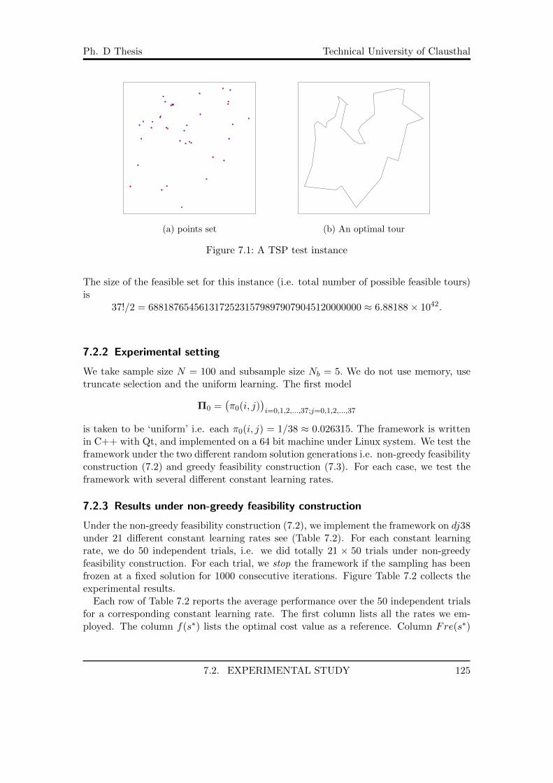
Ph. D Thesis Technical University of Clausthal
(a) points set (b) An optimal tour
Figure 7.1: A TSP test instance
The size of the feasible set for this instance (i.e. total number of possible feasible tours)is
37!/2 = 688187654561317252315798979079045120000000 ≈ 6.88188× 1042.
7.2.2 Experimental setting
We take sample size N = 100 and subsample size Nb = 5. We do not use memory, usetruncate selection and the uniform learning. The first model
Π0 =(π0(i, j)
)i=0,1,2,...,37;j=0,1,2,...,37
is taken to be ‘uniform’ i.e. each π0(i, j) = 1/38 ≈ 0.026315. The framework is writtenin C++ with Qt, and implemented on a 64 bit machine under Linux system. We test theframework under the two different random solution generations i.e. non-greedy feasibilityconstruction (7.2) and greedy feasibility construction (7.3). For each case, we test theframework with several different constant learning rates.
7.2.3 Results under non-greedy feasibility construction
Under the non-greedy feasibility construction (7.2), we implement the framework on dj38under 21 different constant learning rates see (Table 7.2). For each constant learningrate, we do 50 independent trials, i.e. we did totally 21 × 50 trials under non-greedyfeasibility construction. For each trial, we stop the framework if the sampling has beenfrozen at a fixed solution for 1000 consecutive iterations. Figure Table 7.2 collects theexperimental results.
Each row of Table 7.2 reports the average performance over the 50 independent trialsfor a corresponding constant learning rate. The first column lists all the rates we em-ployed. The column f(s∗) lists the optimal cost value as a reference. Column Fre(s∗)
7.2. EXPERIMENTAL STUDY 125

Ph. D Thesis Technical University of Clausthal
cities xi (x-coordinate) yi (y-coordinate)
0 11003.611100 42102.500000
1 11108.611100 42373.888900
2 11133.333300 42885.833300
3 11155.833300 42712.500000
4 11183.333300 42933.333300
5 11297.500000 42853.333300
6 11310.277800 42929.444400
7 11416.666700 42983.333300
8 11423.888900 43000.277800
9 11438.333300 42057.222200
10 11461.111100 43252.777800
11 11485.555600 43187.222200
12 11503.055600 42855.277800
13 11511.388900 42106.388900
14 11522.222200 42841.944400
15 11569.444400 43136.666700
16 11583.333300 43150.000000
17 11595.000000 43148.055600
18 11600.000000 43150.000000
19 11690.555600 42686.666700
20 11715.833300 41836.111100
21 11751.111100 42814.444400
22 11770.277800 42651.944400
23 11785.277800 42884.444400
24 11822.777800 42673.611100
25 11846.944400 42660.555600
26 11963.055600 43290.555600
27 11973.055600 43026.111100
28 12058.333300 42195.555600
29 12149.444400 42477.500000
30 12286.944400 43355.555600
31 12300.000000 42433.333300
32 12355.833300 43156.388900
33 12363.333300 43189.166700
34 12372.777800 42711.388900
35 12386.666700 43334.722200
36 12421.666700 42895.555600
37 12645.000000 42973.333300
Table 7.1: Point sets for test instance
7.2. EXPERIMENTAL STUDY 126
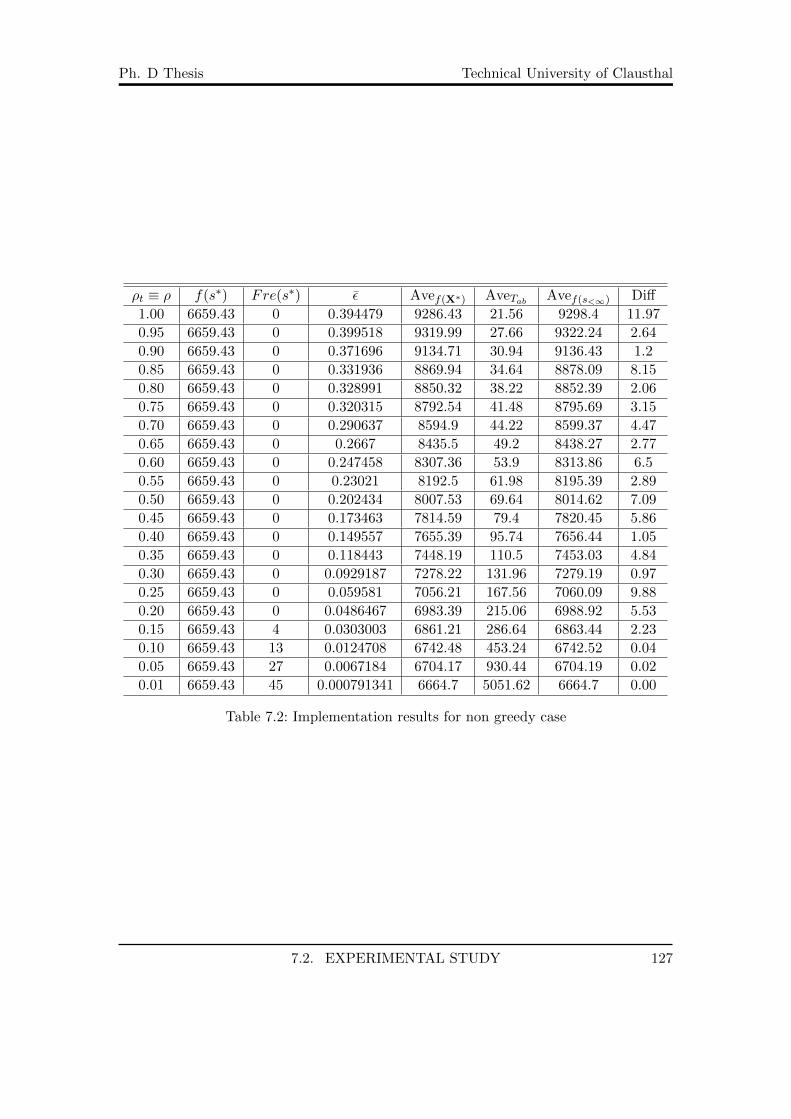
Ph. D Thesis Technical University of Clausthal
ρt ≡ ρ f(s∗) Fre(s∗) ε Avef(X∗) AveTab Avef(s<∞) Diff
1.00 6659.43 0 0.394479 9286.43 21.56 9298.4 11.97
0.95 6659.43 0 0.399518 9319.99 27.66 9322.24 2.64
0.90 6659.43 0 0.371696 9134.71 30.94 9136.43 1.2
0.85 6659.43 0 0.331936 8869.94 34.64 8878.09 8.15
0.80 6659.43 0 0.328991 8850.32 38.22 8852.39 2.06
0.75 6659.43 0 0.320315 8792.54 41.48 8795.69 3.15
0.70 6659.43 0 0.290637 8594.9 44.22 8599.37 4.47
0.65 6659.43 0 0.2667 8435.5 49.2 8438.27 2.77
0.60 6659.43 0 0.247458 8307.36 53.9 8313.86 6.5
0.55 6659.43 0 0.23021 8192.5 61.98 8195.39 2.89
0.50 6659.43 0 0.202434 8007.53 69.64 8014.62 7.09
0.45 6659.43 0 0.173463 7814.59 79.4 7820.45 5.86
0.40 6659.43 0 0.149557 7655.39 95.74 7656.44 1.05
0.35 6659.43 0 0.118443 7448.19 110.5 7453.03 4.84
0.30 6659.43 0 0.0929187 7278.22 131.96 7279.19 0.97
0.25 6659.43 0 0.059581 7056.21 167.56 7060.09 9.88
0.20 6659.43 0 0.0486467 6983.39 215.06 6988.92 5.53
0.15 6659.43 4 0.0303003 6861.21 286.64 6863.44 2.23
0.10 6659.43 13 0.0124708 6742.48 453.24 6742.52 0.04
0.05 6659.43 27 0.0067184 6704.17 930.44 6704.19 0.02
0.01 6659.43 45 0.000791341 6664.7 5051.62 6664.7 0.00
Table 7.2: Implementation results for non greedy case
7.2. EXPERIMENTAL STUDY 127
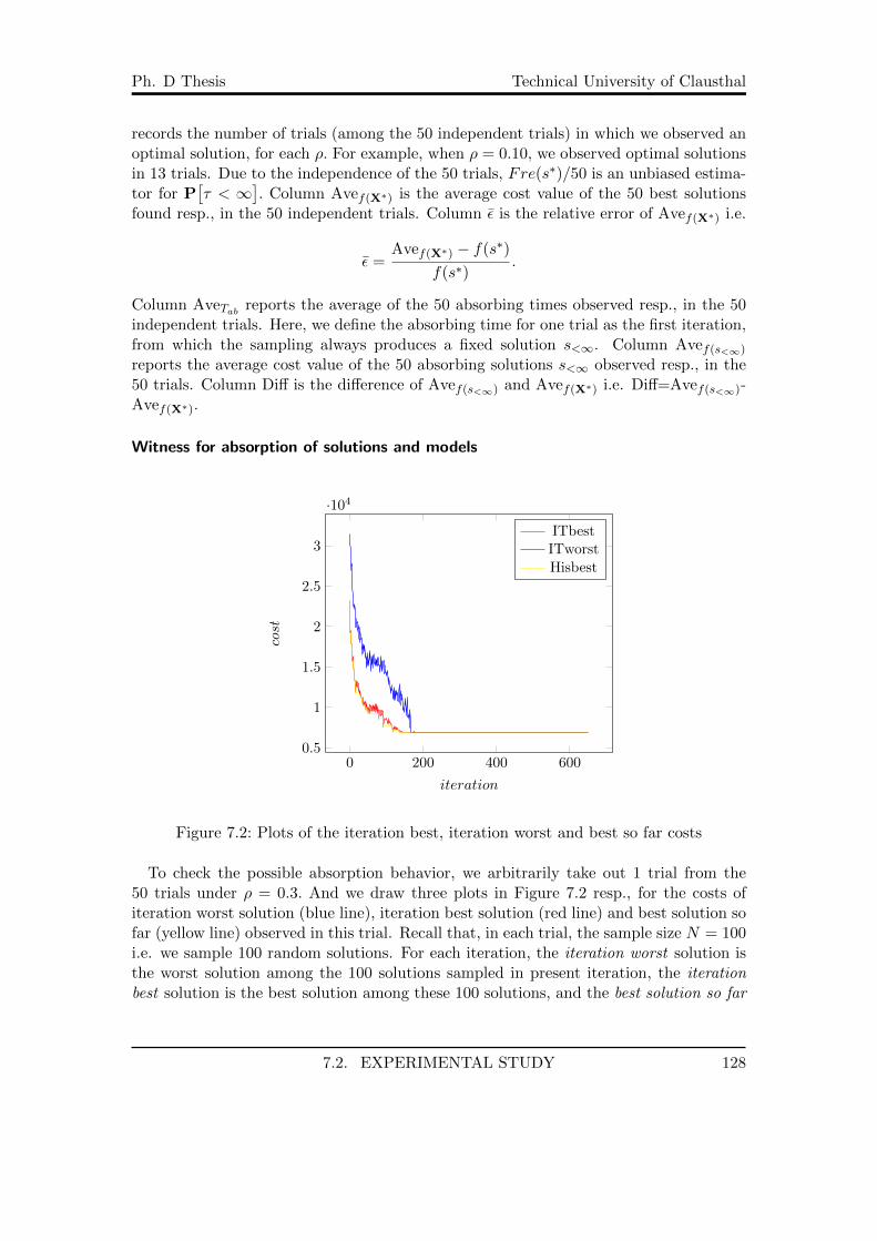
Ph. D Thesis Technical University of Clausthal
records the number of trials (among the 50 independent trials) in which we observed anoptimal solution, for each ρ. For example, when ρ = 0.10, we observed optimal solutionsin 13 trials. Due to the independence of the 50 trials, Fre(s∗)/50 is an unbiased estima-tor for P
[τ < ∞
]. Column Avef(X∗) is the average cost value of the 50 best solutions
found resp., in the 50 independent trials. Column ε is the relative error of Avef(X∗) i.e.
ε =Avef(X∗) − f(s∗)
f(s∗).
Column AveTab reports the average of the 50 absorbing times observed resp., in the 50independent trials. Here, we define the absorbing time for one trial as the first iteration,from which the sampling always produces a fixed solution s<∞. Column Avef(s<∞)
reports the average cost value of the 50 absorbing solutions s<∞ observed resp., in the50 trials. Column Diff is the difference of Avef(s<∞) and Avef(X∗) i.e. Diff=Avef(s<∞)-Avef(X∗).
Witness for absorption of solutions and models
0 200 400 6000.5
1
1.5
2
2.5
3
·104
iteration
cost
ITbestITworstHisbest
Figure 7.2: Plots of the iteration best, iteration worst and best so far costs
To check the possible absorption behavior, we arbitrarily take out 1 trial from the50 trials under ρ = 0.3. And we draw three plots in Figure 7.2 resp., for the costs ofiteration worst solution (blue line), iteration best solution (red line) and best solution sofar (yellow line) observed in this trial. Recall that, in each trial, the sample size N = 100i.e. we sample 100 random solutions. For each iteration, the iteration worst solution isthe worst solution among the 100 solutions sampled in present iteration, the iterationbest solution is the best solution among these 100 solutions, and the best solution so far
7.2. EXPERIMENTAL STUDY 128

Ph. D Thesis Technical University of Clausthal
represents the best solution among all the solutions sampled in previous iterations aswell as the present iteration. Obviously, these three solutions may vary as iterations.The three plots in Figure 7.2 shows resp., the variations in their costs as iterations. Thex-axis represents the iteration, and y-axis represents the cost value. The three solutionshave different costs in beginning. And all the three costs decrease as time goes. Thethree lines then coincide in an iteration near iteration 200 i.e. the costs become identicalfrom then on. Hence, the 100 solutions sampled in iteration t ≥ 200 are always of a fixedcost. This gives an initial impression on absorption of solutions. However, this is notsufficient to be a witness for absorption of solutions, since different solutions may have asame cost value. To clearly demonstrate the absorptions, we also take out six iterations,i.e. iterations 0, 50, 100, 150, 200, 300, in this trial. For each of the selected 6 iterations,we draw two pictures, one for the 100 tours (solutions) sampled in that iteration and theother one for the underlying models producing these solutions. We collect the resulted12 pictures in Figures 7.3-7.4.
For each iteration, we draw the 100 tours according to the points set in Table 7.1together in one picture, and we draw the corresponding model as a plot in anotherpicture. Recall that, the model for iteration t is
Πt =(πt(i, j)
)i,j=0,1,2,...,37
.
In the plot, we further encode each arc (i, j) as an integer 38× i+ j, and use this integeras the x-axis and the probability πt(i, j) as y-axis. If absorption of solutions holds, thenthe 100 tours should finally become identical, and show only one tour in the picture.And if absorption of models holds, the models should finally become a binary string,and show several vertical lines of length 1 in the picture.
Initially, we take a uniform model i.e. π0(i, j) ≡ 1/38, therefore the plot of the modelis a horizontal line, see Figure 7.3 (b). As a result, the 100 tours for iteration 0 is purelyrandomly generated, therefore they show a rather disorganized appearance in Figure 7.3(a). When t = 50, the model shows a clear tendency to be a binary string (see Figure 7.3(d)), and many arcs on the 100 sampled solutions coincide (see 7.3 (c)). When t = 100,the model show a more clear tendency to be a binary string (see 7.3 (f)), and more arcson 100 solutions sampled in this iteration coincide (see 7.3 (e)).
When t = 150, the model almost becomes a binary string (see 7.4 (b)), and mostarcs on 100 solutions in this iteration coincide except for few arcs in the left top corner(see 7.4 (a)). When t = 200, absorption of solutions has already occurred i.e. the 100solutions become identical (see 7.4 (c)), the model approximates a binary string (see 7.4(d)). The pictures for iteration 300 are the same as the pictures for iteration 200, seeFigure 7.4 (e)-(f). This further confirms the absorption of solutions and models.
7.2. EXPERIMENTAL STUDY 129
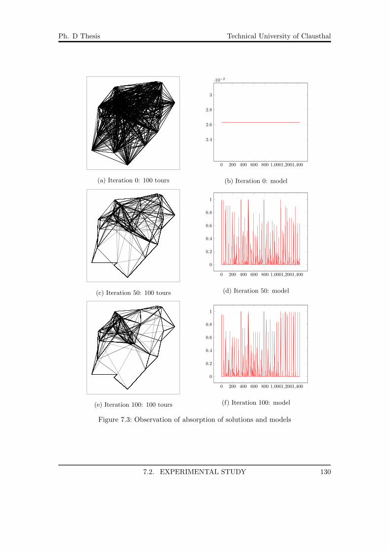
Ph. D Thesis Technical University of Clausthal
(a) Iteration 0: 100 tours
0 200 400 600 800 1,0001,2001,400
2.4
2.6
2.8
3
·10−2
(b) Iteration 0: model
(c) Iteration 50: 100 tours
0 200 400 600 800 1,0001,2001,400
0
0.2
0.4
0.6
0.8
1
(d) Iteration 50: model
(e) Iteration 100: 100 tours
0 200 400 600 800 1,0001,2001,400
0
0.2
0.4
0.6
0.8
1
(f) Iteration 100: model
Figure 7.3: Observation of absorption of solutions and models
7.2. EXPERIMENTAL STUDY 130
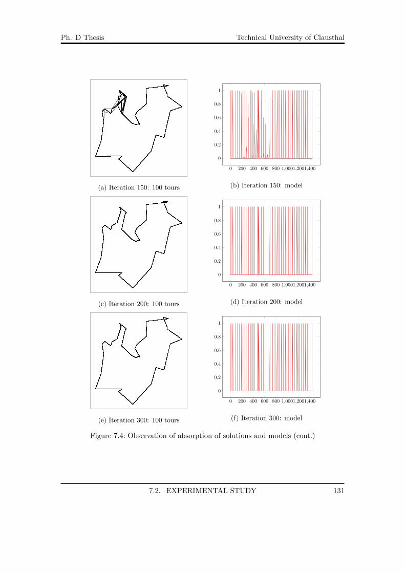
Ph. D Thesis Technical University of Clausthal
(a) Iteration 150: 100 tours
0 200 400 600 800 1,0001,2001,400
0
0.2
0.4
0.6
0.8
1
(b) Iteration 150: model
(c) Iteration 200: 100 tours
0 200 400 600 800 1,0001,2001,400
0
0.2
0.4
0.6
0.8
1
(d) Iteration 200: model
(e) Iteration 300: 100 tours
0 200 400 600 800 1,0001,2001,400
0
0.2
0.4
0.6
0.8
1
(f) Iteration 300: model
Figure 7.4: Observation of absorption of solutions and models (cont.)
7.2. EXPERIMENTAL STUDY 131

Ph. D Thesis Technical University of Clausthal
Relation between ρ and the best found solution
According to Table 7.2, we draw resp., a plot for ρ and the average best found costAvef(X∗) in Figure 7.5 (a), a plot for ρ and the average relative error ε in Figure 7.5(b), and a plot for ρ and Fres∗ (i.e. the number of trials in which optimal solutionsoccurred) in Figure 7.5 (c).
0 0.2 0.4 0.6 0.8 1
7,000
8,000
9,000
ρ
costs
AvBestOptimum
(a) for Avef(X∗)
0 0.2 0.4 0.6 0.8 1
0
0.1
0.2
0.3
0.4
ρε
AvBest
(b) for ε
0 0.2 0.4 0.6 0.8 1
0
10
20
30
40
50
ρ
Occurrence
opt
(c) for Fres∗
Figure 7.5: Relation of ρ and best found solution
In Figure 7.5 (a), the red straight line indicating the optimal value 6659.43. The blueline represents the average best found cost Avef(X∗). Figure 7.5 (a) and (b) clearly showsthat as ρ → 0, the best found solution will approximate optimal solutions. This meansthat we may improve the practical performance for an MBS by reducing the constantlearning rate. It is interesting that the best solution cost almost linearly decreases as ρincreases.
By 7.5 (c), we see that when ρ→ 0, F res∗ → 50. This experimentally demonstratesTheorem 5.7 c). In particular, we see that with a relatively large ρ (≥ 0.20), we are notable to see an optimal solution in the 50 trials. And when the ρ reaches the threshold0.15 (see Table 7.2), Fres∗ increases rapidly as ρ decreases.
7.2. EXPERIMENTAL STUDY 132

Ph. D Thesis Technical University of Clausthal
Relation between ρ, s<∞ and the absorbing time
In the above, we have demonstrated a typical absorption behavior of the solutions andmodels. To give more insight to the qualities of absorbing solutions s<∞ and absorbingtime, we draw resp., a plot for ρ and the average absorbing cost Avef(s<∞) in Figure7.6 (a), a plot for ρ and the average absorbing time AveTab in Figure 7.6 (b), and aplot for ρ and Diff in Figure 7.6 (c). In (a), the red line again indicates the optimum
0 0.2 0.4 0.6 0.8 1
7,000
8,000
9,000
ρ
costs
AvAbValueOptimum
(a) for Avef(s<∞)
0 0.2 0.4 0.6 0.8 1
0
2,000
4,000
ρT
(b) for AveTab
0 0.2 0.4 0.6 0.8 1
0
5
10
ρ
¯s <∞
−X∗
(c) for Diff=Avef(s<∞) −Avef(X∗)
Figure 7.6: ρ and absorption
6659.43, the blue line is the average absorbing cost value Avef(s<∞). It is surprising thatAvef(s<∞) also approximates optimum as ρ→ 0. This means that the absorbing solutionmay become an optimal solution if we employ a small enough ρ.
Absorbing time is the first iteration from which the sampling will be frozen at a fixedsolution i.e. s<∞. Therefore, it directly affects the total number of different solutionsthe framework can visit. From Figure 7.6 (b), we see that the average absorption timeAveTab increases as ρ → 0. So, decreasing ρ may increase the search capacity i.e. thetotal number of possible solutions the framework can visit. When ρ < 0.15 (see Table7.2), AveTab increases dramatically as ρ decreases. For ρ ≥ 0.15, it changes moderately
7.2. EXPERIMENTAL STUDY 133

Ph. D Thesis Technical University of Clausthal
ρt ≡ ρ f(s∗) Fre(s∗) ε Avef(X∗) AveTab Avef(s<∞) Diff
1.00 6659.43 0 0.00556045 6696.46 3.78 6696.46 0.00
0.95 6659.43 7 0.00329671 6681.38 9.1 6681.38 0.00
0.90 6659.43 11 0.00281658 6678.19 9.74 6678.19 0.00
0.85 6659.43 10 0.00182641 6671.59 13.78 6671.59 0.00
0.80 6659.43 13 0.00203408 6672.98 15.42 6672.98 0.00
0.75 6659.43 17 0.00105385 6666.45 17.76 6666.45 0.00
0.70 6659.43 19 0.00182242 6671.57 19.3 6671.57 0.00
0.65 6659.43 24 0.000857031 6665.14 22.5 6665.14 0.00
0.60 6659.43 29 0.000586001 6663.33 25.6 6663.33 0.00
0.55 6659.43 32 0.00039527 6662.06 28.56 6662.06 0.00
0.50 6659.43 36 0.00025947 6661.16 31.94 6661.16 0.00
0.45 6659.43 41 0.000119201 6660.22 37.44 6660.22 0.00
0.40 6659.43 44 7.92956e-05 6659.96 43.58 6659.96 0.00
0.35 6659.43 46 5.53364e-05 6659.8 49.78 6659.8 0.00
0.30 6659.43 46 5.64757e-05 6659.81 62.7 6659.81 0.00
0.25 6659.43 49 1.42916e-05 6659.53 79.66 6659.53 0.00
0.20 6659.43 50 0 6659.43 105.18 6659.43 0.00
0.15 6659.43 50 0 6659.43 167.92 6659.43 0.00
0.10 6659.43 50 0 6659.43 347.36 6659.43 0.00
Table 7.3: Implementation results for greedy case
as ρ. And when ρ > 0.20, it is smaller than 200, see Table 7.2. Therefore, the searchcapacity is at most 2 × 10⁴, i.e. the framework can visit at most (200 × 100) differenttours, in this case. Compared to the size 6.88188 × 1042 of underlying feasible set, thisnumber is extremely small. This may mean that the framework can be rather efficientwhen ρ > 0.2. However, we did not see an optimal solution in this case, see Table 7.2.To balance the efficiency and effectiveness, we would recommend to set ρ = 0.05 underwhich we observed optimal solutions in 27 trials and the average absorbing time is 930.44i.e. the search capacity is 9.3× 10⁴, see Table 7.2.
Figure 7.6 (c) shows the difference between the average absorbing cost and the averagebest found cost i.e. Avef(s<∞) − Avef(X∗). We see that this difference is generally notequivalent to 0. Therefore, the absorbing solution is generally not the same as the bestsolution found. However, when ρ small enough (< 0.2), the two costs may coincide. So,the two solutions may be the same for small ρ. This is an interesting phenomenon.
7.2.4 Under greedy feasibility construction
For the greedy feasibility construction, we take 19 different constant learning rates.For each learning rate, we also do 50 independent trials. Table 7.3 above shows theexperimental results.
A significant difference with Table 7.2 is that the Column Diff in this case all become 0.
7.2. EXPERIMENTAL STUDY 134

Ph. D Thesis Technical University of Clausthal
This means that under greedy feasibility construction, the absorbing solutions are morelikely to be the best solution found. The second significant difference is Column Fre(s∗)are almost filled by positive integers. This means the greedy feasibility constructionsignificantly increases the occurring probability of optimal solutions.
Relation between ρ and best found solution
0.2 0.4 0.6 0.8 1
6,660
6,670
6,680
6,690
6,700
ρ
costs
AvBestOptimum
(a) for Avef(X∗)
0.2 0.4 0.6 0.8 1
0
2
4
6·10−3
ρ
ε
(b) for ε
0.2 0.4 0.6 0.8 1
0
20
40
ρ
occurrence
(c) for Fres∗
Figure 7.7: ρ and best found solution for greedy case
Figure 7.7 is drawn according to Table 7.3. Picture (a) shows the plot of the averagebest found cost Avef(X∗). Picture (b) shows the plot for the relative error. Picture (c)shows the plot for the total number of trials among the 50 independent trials in whichwe observed an optimal solution.
According to Figure 7.7 (a)-(b), we see that under greedy feasibility construction, theaverage best found cost Avef(X∗) is very close to the optimum. In (a), the red horizontalline again indicates the optimum, and the blue line represents Avef(X∗). We see also thatAvef(X∗) approximates optimum as ρ decreases. The maximal average relative error is
7.2. EXPERIMENTAL STUDY 135

Ph. D Thesis Technical University of Clausthal
less than 6 × 10⁻³, see (b). Moreover, by Figure 7.7 (c), we see that the probabilityP[τ <∞] may also approximate 1.0 as ρ decreases.
0.2 0.4 0.6 0.8 1
6,660
6,670
6,680
6,690
6,700
ρ
costs
AvAbValueoptimum
(a) for Avef(s<∞)
0.2 0.4 0.6 0.8 1
0
100
200
300
ρ
T
avabiter
(b) for AveTab
0.2 0.4 0.6 0.8 1
−0.5
0
0.5
1
ρ
¯s<∞−X
∗
(c) for Diff=Avef(s<∞) −Avef(X∗)
Figure 7.8: ρ and absorption for greedy case
ρ and absorption
Figure 7.8 is also drawn according to Table 7.3. Picture (a) shows the plot for theaverage absorbing cost Avef(s<∞). Picture (b) shows the plot for the average absorbingtime. Picture (c) shows the plot for the difference between the average best found costand the average absorbing cost.
We can see from Figure 7.8 (a) that the average absorbing cost also decreases as ρdecreases. And it approximates the optimum when ρ is smaller enough. By (b), theaverage absorbing time increases as ρ decreases. So, in the greedy feasibility case, thesearch capacity also increases as ρ decreases. When ρ is small (ρ < 0.2), the time mayalso increase dramatically. It is interesting that in the greedy case, the absorbing cost isalways the same as the best found cost, see (c). Therefore, the absorbing solution maybe the best found solution.
7.2. EXPERIMENTAL STUDY 136

Ph. D Thesis Technical University of Clausthal
0 0.2 0.4 0.6 0.8 1
7,000
8,000
9,000
ρ
costs
GreedyNon-Greedy
(a) comparison for Avef(X∗)
0 0.2 0.4 0.6 0.8 1
0
5
10
ρ
¯s<∞−X
∗
GreedyNon-Greedy
(b) comparison for Diff
0 0.2 0.4 0.6 0.8 1
0
20
40
ρ
occurrence
GreedyNon-Greedy
(c) comparison for Fres∗
0 0.2 0.4 0.6 0.8 1
0
2,000
4,000
ρ
T
GreedyNon-Greedy
(d) comparison for AveTab
Figure 7.9: Comparison
Compare with non-greedy case
According to Tables 7.2-7.3, we draw four pictures in Figure 7.9 for a comparison ofgreedy and non-greedy feasibility constructions. Picture (a) shows the plots for averagebest found costs in the two cases respectively, picture (b) shows the plots for the differencebetween average best found cost and average absorbing cost, picture (c) shows the plotsfor Fres∗s, and picture (d) shows the plots for average absorbing times. In eachpicture, we use red line to indicate the greedy case, and blue line to indicate the non-greedy case.
By (a), we see that the greedy feasibility construction significantly improves the per-formance i.e. the average best found cost (red) in greedy case is significantly lower thanaverage best found cost (blue) in the non-greedy case. In the picture, the red line isalmost a horizontal line, since it is almost an optimum compared to the non-greedy case.
By (b), we see that the average absorbing cost is significantly different with the averagebest found cost in the non-greedy case (see blue line). However, the average absorbingcost is the same as the average best found cost in the greedy case (see red line). There-
7.2. EXPERIMENTAL STUDY 137

Ph. D Thesis Technical University of Clausthal
fore, with greedy feasibility construction, the absorbing ‘accuracy’ is also significantlyimproved.
By (c), we see that the greedy feasibility construction may also increase the occurringprobability of optimal solutions. However, when ρ is small enough, the advantage ofgreedy feasibility construction will be no longer significant.
By (d), the average absorbing time in greedy case is always smaller than in the non-greedy case. Therefore, greedy feasibility construction may be more efficient. To furthercompare the efficiencies of the two cases, we define the relative efficiency of greedyfeasibility construction for a constant ρ as
average absorbing time in non-greedy− average absorbing time in greedy
average absorbing time in greedy.
For example, when ρ = 1.0, the average absorbing times are 21.56 in non-greedy caseand 3.78 in greedy case, so the relative efficiency of greedy feasibility construction is
21.56− 3.78
3.78≈ 4.7037,
see Tables 7.2-7.3 for the values. Note that, the average absorbing time is a very impor-tant index for the search capacity i.e. the total number of possible feasible solutions theframework can visit. Therefore, it may reflect the efficiency. By checking the two Tablesmore closely, we find that the relative efficiency may decrease as ρ decreases. We cansee that when ρ = 0.6, the relative efficiency is about 1.1055, when ρ = 0.10, the relativeefficiency is about 0.3048. Therefore, when ρ is smaller, the relative efficiency of thegreedy feasibility construction may be no longer significant. So, we would recommend arelatively big ρ in the greedy case. To balance the efficiency and effectiveness, we wouldrecommend ρ = 0.5 in the greedy case, by which we observed optimal solutions in 36trials and the relative efficiency is 1.1803.
7.2. EXPERIMENTAL STUDY 138
8 Summary and future work
In this Thesis, we investigated some important asymptotic properties for model-basedheuristics in combinatorial optimization. To facilitate our analysis, we proposed a unifiedframework for model-based algorithms. In particular, we introduced a sampling mech-anism called feasibility construction. It can unify the samplings in those model-basedalgorithms used in practice. More importantly, it can introduce some greediness anddependencies into the sampling.
To give some insight to the effectiveness of model-based search, we showed conditionsfor guaranteeing to find an optimal solutions. The conditions did not assume a particularstructure of the underlying problem. Therefore, they may apply to all combinatorial op-timization problems. For some test problems, we also proposed conditions for efficientlyreaching an optimal solution.
In the asymptotic analysis of the underlying solutions, we found that the famousgenetic drift may also hold in model based search. In particular, we found that the sam-pling in model-based search may stick on a fixed solution after finitely many iterations.Moreover, the solution freezing the sampling is generally of a high quality compared tothose solutions seen in history.
In model based search, the asymptotic property of the models is of great importance.By our analysis, we found conditions which make the models converge to a limit con-centrating on some optimal solution. However, for the memoryless case, we are not ableto show a similar condition. But, our former work has shown that absorption of modelsand finite reachability are also compatible in this case.
By implementing the framework on a TSP instance, we are able to verify most of thefindings. In particular, we found that the performance can be significantly improved ifwe use a ‘good’ greedy information in the feasibility construction. Moreover, we foundthat the absorbing solution can be improved if we use a small learning rate, and theabsorbing time increases as the learning rate decreases. Therefore, higher learning ratemay make the framework rather efficient. However, the quality of best solution foundmay be lower in this case.
As we mentioned, in the non-memory case, we are not able to show a condition whichmakes the models converge to a limit concentrating on optimal solutions. So, it shouldbe an interesting topic for a future work. Note that this is an important issue for thecross entropy algorithm both in combinatorial optimization and in rare event simulation.
In Subsection 4.2.4, we said that the feasibility construction can introduce probabilisticdependencies into the sampling. The greedy information in TSP actually reflects somepriori probabilistic dependencies. In the experimental study, we have seen that greedyfeasibility construction indeed significantly improves the average performance. However,many practical problems may not have such a priori greedy information available. So,
139

Ph. D Thesis Technical University of Clausthal
another possibly future work is to learn empirical greedy information from a collection ofbest solutions found in history, and then incorporate it into the feasibility construction.This should be a topic closely related to the field of linkage learning.
In this Thesis, we investigated the runtime only on some rather simple problems.Due to simply structure, the results may not apply to practical problems. Therefore,a future work on runtime analysis should concern runtime results on some practicalproblems like TSP, scheduling, assignment etc. And the results may have significantlymeaning in practice.
140

Appendix
A.1 Some definitions in graph theory
Graphs are fundamental structures in CO. In this section, we collect some elementaryconcepts and notations of graphs. All the materials we show here can be also found insome standard textbooks for CO, see e.g. Korte et al[KV02] Chapter 2.
Given V a finite set, and E ⊆ (c, d)|c ∈ V and d ∈ V . Then, we call the pairG = (V,E) as a graph, and each element in V as a node or vertex. Furthermore, if Esatisfies the condition that,
∀c, d ∈ V, (c, d) ∈ E ⇐⇒ (d, c) ∈ E,
we call G as an undirected graph, otherwise G is called as a directed graph. For anundirected graph G, we call each element in E as an edge. For a directed graph G, wecall each element in E as an arc. Let e = (v1, v2) be an edge (an arc in the directedcase correspondingly), then we say that vertices v1 and v2 are adjacent. v1 is a neighborof v2 (and vice verse). v1 and v2 are called endpoints of e. In the directed case, we saythat e leaves v1 and enters v2. Two edges or arcs which share at least one endpoint areadjacent. And if a vertex is an endpoint of an edge, we say that it is incident with theedge. Then, for an arbitrary vertex, we can define its degree as the number of edges (orarcs) which are incident to it. And in the directed case, we can define the out-degree of avertex as the number of arcs leaving it and the in-degree as the number of arcs enteringit.
A walk W on a graph G = (V,E) is a sequence v1, e1, v2, . . . , vk, ek, vk+1 with
• vi ∈ V for all i = 1, . . . , k + 1,
• ei = (vi, vi+1) ∈ E for all i = 1, . . . , k,
• ei 6= ej for all i 6= j and i, j ∈ 1, . . . , k.Obviously, a walk can also be represented as a sequence of vertices or a sequence of edges(arcs). And if W = (v1, e1, v2, . . . , vk, ek, vk+1) is a walk, then we call v1 and vk+1 asthe endpoints in the undirected case, we call v1 as the start point and vk+1 as the endpoint in the directed case. We say a walk is closed if the endpoints (start and end pointin the directed case) are the same. A path is a walk with different vertices, i.e. a walk(v1, e1, v2, . . . , vk, ek, vk+1) with vi 6= vj for i 6= j. And a circuit or circle is a closed path,i.e. the underlying walk is closed.
A subgraph G1 = (V1, E1) of G = (V,E) is a graph such that V1 ⊆ V and E1 ⊆ E.And if V1 = V, we say that G1 is a spanning subgraph of G. Then a spanning walk (pathand circuit resp.) is a walk which contains all possible vertices on G, and a Hamiltoniancircle or tour is a spanning circuit on G.
141

Ph. D Thesis Technical University of Clausthal
Assume G = (V,E) is a graph, and w : E 7→ R is a real function defined on the set ofedges or arcs, then we call the triple (V,E,w) as a weighted graph, and w as a weightfunction of graph G.
Suppose G = (V,E) is an undirected graph, we say it is connected if for any twovertices v1 and v2, we can find a path with v1 and v2 as endpoints. And we say that Gis fully or completely connected if and only if for any two vertices a and b in V, we have(a, b) ∈ E. Evidently, fully connected implies connected.
In undirected case, a forest is a graph without circuits. And a connected forest iscalled a tree. A vertex in a tree with degree 1 is called a leaf. And in the directed case, aroot on a tree is a vertex which has 0 in-degree. Then a branch can be formally definedas a path which leaves the root and enters a leaf.
142

Ph. D Thesis Technical University of Clausthal
A.2 Shannon Entropy, K-L divergence and importance sampling
This section proposes some terminologies in information theory. Elements in this sectioncan also be found in Cover et al[CT12] and Rubinstein et al[RK04].
In information theory, Shannon entropy or entropy is the most celebrated measure ofuncertainty. Let X be a random variable with density f . Then the Shannon entropy orentropy of X is defined as
E(X) := E[ln( 1
f(X)
)]= −E
[lnf(X)
]= −
∫f(x)lnf(x)dx.
Obviously, if X concentrates on one value, i.e. P(X = a) = 1 for some constant valuea, then E(X) = 0. And if X is uniform distributed, E(X) reaches maximum.
Similarly, we can define the joint or total entropy E(X1, . . . , Xm) of random variablesX1, . . . , Xm with joint density f(x1, . . . , xm) as
E(X1, X2, . . . , Xm) := −∫f(x1, x2, . . . , xm)lnf(x1, x2, . . . , xm)dx1dx2 · · · dxm.
It measures the ‘joint’ or ‘total’ uncertainty of random variables X1, . . . , Xm.For two random variables X1 and X2 with joint density f, we can reasonably define
the conditional entropy of X1 given X2 as
E(X1|X2) := E(X1, X2)− E(X2) = −E[lnf(X1, X2)
fX1(X1)
],
where fX1(·) is the marginal density of X1. Note that the conditional entropy measuresthe remaining uncertainty when X2 is given.
To measure the mutual dependency of two random variables, we define the mutualinformation I(X1, X2) of two random variables with joint density f as
I(X1, X2) := E(X1) + E(X2)− E(X1, X2) = E(X1)− E(X1|X2) = E(X2)− E(X2|X1).
Two basic facts about mutual information is that
• I(X1, X2) = I(X2, X1),
• I(X1, X2) = 0 ⇐⇒ X1 and X2 are probabilistically independent.
The Kullback-Leibler divergence is a ‘metric’ of densities. It can be used to measurethe ‘distance’ of two probability densities. Let g and f be two densities with respect to ameasure µ on a space X. The Kullback-Leibler divergence (K-L divergence) of f respectto g is
D(f ; g) := Eg
[lng(X)
f(X)
]=
∫−g(x)lnf(x)dx−
∫−g(x)lng(x)dx.
Where Eg(·) indicates that the expectation is respect to density g. It is easy to checkthat D(f ; g) ≥ 0, and D(f ; g) = 0 if and only if f = g, µ- almost surely. D(·; ·) is alsocalled cross entropy or relative entropy.
143

Ph. D Thesis Technical University of Clausthal
A.3 Linear programming and integer programming
Linear programming optimization (LPO, see [KV02] p. 49) concerns solving problemslike
minimizing: cTx,
subject to: Ax ≤ b,x ∈ Rn,
where matrix A ∈ Rm×n, column vector b ∈ Rm and column vector c ∈ Rn are constant.A LPO instance is called a linear program (LP). And most of the COPs can be formulatedas LPs.
Integer programming optimization (IPO, see [KV02] p. 91) can be seen as a subtopic ofLPO which concerns solving the LPs with A ∈ Zm×n, b ∈ Zm and x, c ∈ Zn. A more re-strictive research topic is zero-one integer programming optimization which concentrateson LPs with A ∈ 0, 1m×n, b ∈ 0, 1m and x, c ∈ 0, 1n. Obviously, zero-one integerprogramming is a subtopic of CO. Actually, due to the convexity of feasible regions,LPO can also be seen as a subtopic of CO.
144

Ph. D Thesis Technical University of Clausthal
A.4 Elements about probability theory and stochastic process
Here, we collect some elements about probability theory and stochastic process, see[Cin75] and [Dur10] for a further reference.
In probability theory, we call a countable or uncountable set Ω as a sample space.Then an element in Ω is called as an outcome, and a subset of Ω is called as a randomevent .
Let B be a collection of random events on a sample space Ω. We say that B is anσ-algebra on Ω if and only if
i) it contains complete event i.e. Ω ∈ B,ii) it is closed under complement i.e. A ∈ B ⇒ Ω−A ∈ B,iii) it is closed under infinite intersection i.e. ∀n ∈ N An ∈ B, ⇒
⋃n∈N
An ∈ B.
And we call pair(Ω,B
)as a measurable space if B is a σ-algebra on Ω. For a measurable
space(Ω,B
), we call each event in B as a B-measurable set. A typical measurable space
is the so-called Borel space. Let Rn = R× · · · × R be the Euclidean space of dimensionn. And Bn denotes the smallest σ-algebra which contains all of open sets in Rn. Thenwe call (Rn,Bn) as the n-dimensional Borel space.
Let(Ω,B
)be a measurable space. Let P : B 7→ [0, 1] be a set function such that
i) P(Ω) = 1,
ii) let Ann∈N be a sequence in B s.t. An ∩Am = ∅ for n 6= m, then
P[ ⋃n∈N
An
]=∑n∈N
P[An],
then P is called a probabilistic measure on(Ω,B
), and triple
(Ω,B,P
)is called a prob-
ability space.Given a probability space
(Ω,B,P
). The probability of a random event A ⊆ Ω is
defined asP(A) := inf
P(B)
∣∣ B ∈ B, A ⊆ B,i.e. the outer measure of A under probabilistic measure P. Note that measurable setmust be a random event, but a random event may not be a measurable set. We say thattwo random events A1 and A2 are independent if
P[A1 ∩A2
]= P
[A1
]·P[A2
].
Suppose P(A) > 0 for A ∈ B. Then the probability of a random event B conditioned onA is defined as
P[B∣∣ A] :=
P[A ∩B
]P[A] .
145
Ph. D Thesis Technical University of Clausthal
A very useful formula about conditional probability is
P[ ⋂t∈N
At]
= P[A0]∞∏t=1
P[At∣∣ ∀m ≤ t− 1 Am
]which is a standard technique for showing the probability of chain events.
Suppose(Ω,B
)is a measurable space. Then we call a function X : Ω 7→ Rn as an
n-dimensional measurable function if for all B ∈ Bn, X−1(B) ∈ B. In probability theory,
we often call a measurable function X as a random variable. And E = X(Ω) ⊆ Rn iscalled the state space of that random variable. For a Borel measurable set B ∈ Bn, anda probabilistic measure P, we write
P[X ∈ B
]:= P
ω ∈ Ω
∣∣ X(ω) ∈ B.
Let X1 and X2 be two random variables, then we say that they are independent if andonly if
P[X1 ∈ B1, X2 ∈ B2
]= P
[X1 ∈ B1
]·P[X2 ∈ B2
]for all B1, B2 ∈ Bn.
Let X is an 1-dimensional random variable on a probability space(Ω,B,P
). Then we
call the functionF(x) := P
[X ≤ x
]for all x ∈ R
as the distribution function of X. And if the state space E of X is countable, sayxi ∈ R | i ∈ N, its distribution function may be described by a vector
(P[X = xi]
)i∈N
i.e.F(x) =
∑xi≤x,xi∈E
P[X = xi].
Suppose (Ωθ,Bθ,Pθ
)θ∈Θ
is a family of probability spaces. We write∏θ∈Θ
Ωθ :=
(ωθ)θ∈Θ
∣∣ ωθ ∈ Ωθ, θ ∈ Θ
as the product sample space. Let∏θ∈Θ Bθ be the smallest σ-algebra on
∏θ∈Θ Ωθ which
contains the collectionC(Aθ1 , . . . , Aθn)
∣∣ Aθ1 ∈ Bθ1 , . . . , Aθn ∈ Bθn , n ∈ N,
whereC(Aθ1 , . . . , Aθn) :=
(ωθ)θ∈Θ
∣∣ ωθ1 ∈ A1, . . . , ωθn ∈ Aθn⊆∏θ∈Θ
Ωθ.
And define∏θ∈Θ Pθ as the unique probabilistic measure on
(∏θ∈Θ Ωθ,
∏θ∈Θ Bθ
)such
that∏θ∈Θ
Pθ
(C(Aθ1 , . . . , Aθn)
)=
n∏i=1
Pθi(Aθi) for all Aθ1 ∈ Bθ1 , . . . , Aθn ∈ Bn with n ∈ N.
146
Ph. D Thesis Technical University of Clausthal
Then the probability space(∏
θ∈Θ Ωθ,∏theta∈Θ Bθ,
∏θ∈Θ Pθ
)is called a product proba-
bility space.Let M be the collection of all possible 1-dimensional random variables on a probability
space(Ω,B,P
). Then we say that a function E : M 7→ R is the expectation operator if
and only if it satisfies
i) for all A ∈ B, E(1A
)= P(A),
ii) if Xn → X as n→∞ and Xn ∈M for all n ∈ N, then E(Xn)→ E(X) as n→∞,iii) for all c ∈ R and X,Y ∈M, E(c ·X) = c ·E(X) and E(X + Y ) = E(X) + E(Y ),
where observe that 1A(ω) ∈M. And note that M is closed under limit. And furthermore,if Ω is countable, then
E(X) =∑ω∈Ω
X(ω)Pω for all X ∈M.
Suppose(Ω,B,P
)is a probability space. Let (Xt)t∈Γ be a sequence of random vari-
ables with a common state space E on it. Then we say (Xt)t∈Γ is a stochastic processwith state space E. And if Γ is countable, we say that (Xt)t∈Γ is discrete parameterprocess.
Let (Xt)t∈N be a discrete process on(Ω,B,P
). Then we say that it is a Markov chain
if and only if
P[Xt+1 ∈ B
∣∣ Xt ∈ Bt, Xt−1 ∈ Bt−1, . . . , X0 ∈ B0
]:= P
[Xt+1 ∈ B
∣∣ Xt ∈ Bt]
for all t ∈ N, all B ∈ Bn, and also all Bi ∈ Bn for i = 0, 1, . . . , t.
147

Ph. D Thesis Technical University of Clausthal
A.5 Useful notations in runtime analysis
Suppose f and g are two positive functions on natural numbers.
Big O notation:
We write f ∈ O(g) if and only if
∃a > 0 ∃N ∈ N ∀n ≥ N f(n) ≤ a · g(n).
Big O notation is used to show that f is bounded above by g asymptotically. Obviously,f ∈ O(g) if and only if limn→∞ sup f(n)/g(n) <∞.
Small o notation:
We write f ∈ o(g) if and only if
∀a > 0 ∃N ∈ N ∀n ≥ N f(n) ≤ a · g(n).
f ∈ o(g) means that f is dominated by g asymptotically. And f ∈ o(g) if and only iflimn→∞ f(n)/g(n) = 0.
Big Ω notation:
We write f ∈ Ω(g) if and only if
∃a > 0 ∃N ∈ N ∀n ≥ N f(n) ≥ a · g(n).
So f ∈ Ω(g) means that f is bounded below by g asymptotically. And f ∈ Ω(g) if andonly if g ∈ O(f).
Small ω notation:
We write f ∈ ω(g) if and only if
∀a > 0 ∃N ∈ N ∀n ≥ N f(n) ≥ a · g(n).
f ∈ ω(g) if and only if f dominates g asymptotically.
Big Θ notation:
We write f ∈ Θ(g) if and only if f ∈ O(g) ∩ Ω(g), namely f is bounded both below andabove by g asymptotically.
∼ notation:
We write f ∼ g if and only if they are asymptotically equivalent i.e.
limn→∞
f(n)
g(n)= 1.
148

Ph. D Thesis Technical University of Clausthal
A.6 Application of cross entropy algorithm in rare event simulation
CE is initially motivated for rare event simulation (RES). As an additional reference onCE, we introduce this in the present Section. For a detailed reference on RES, see thebook [RT+09].
A.6.1 A brief introduction to rare event simulation
Generally, a rare event is an event which occurs with an extremely small probability. Forexample, a catastrophic failure for a civil aircraft during a flight is generally a rare event.As a security or reliability assessment, we may need to calculate or estimate occurringprobabilities of some ‘unpleasant’ rare events for a complex system in practice.
Typically, we may need to calculate a probability
P(A) =
∫(x1,...,xn)∈Ω
1f(y1,...,yn)≤γ(x1, . . . , xn)g(x1, . . . , xn)dx1 · · · dxn (1)
where n ∈ N is a fixed integer and A is a rare event of form[f(X1, . . . , Xn
)≤ γ
](2)
for a fixed threshold value γ ∈ R, random variables X1, . . . , Xn with joint densityg(x1, . . . , xn) and state space Ω, and f : Ω 7→ R is a performance function. Here, anelement x = (x1, . . . , xn) ∈ Ω corresponds to a state for a system, and a failure occurs ifthe system is in a state x ∈ Ω with performance value f(x) ≤ γ.
In theory, we can estimate (1) by the so-clalled crude monte-carlo method (see Ap-pendix A. 2 or [RT+09] pp. 2-4), and the corresponding estimator is
P(A) =1
N
N∑j=1
1(−∞,γ]
(f(X(j)(1), . . . ,X(j)(n)
)), (3)
where X(1) =(X(1)(1), . . . ,X(1)(n)
), . . . ,X(N) =
(X(N)(1), . . . ,X(N)(n)
)are i.i.d from
density g. Estimator (3) has a coefficient of variation (c.v.)√Var
[P(A)
]E[P(A)
] =
√(1−P(A)
)N ·P(A)
.
When P(A)
is not too small, we can make the above c.v. in a tolerant level by takinga sufficiently large N. However, the A here is a rare event. To get an effective approxi-mation to (1), we may need an extremely huge N. For example, P(A) may be smallerthan 10−9, then we have to take an N ≥ 1013 so as to make the c.v. smaller than 0.01.Obviously, this is prohibitive in practice.
In RES, we concern how to estimate (1) or simulate A effectively for the case that P(A)
is extremely small. Importance sampling and splitting techniques are the most frequentlyused approaches in RES. Here, we shall concentrate only on importance sampling. Forthe splitting techniques, see [RT+09] Chapter 2 of Part I for an introduction.
149

Ph. D Thesis Technical University of Clausthal
A.6.2 Importance Sampling
Let x = (x1, . . . , xn), y = (y1, . . . , yn) and X = (X1, . . . , Xn). Then, (1) can be writtenas
P(A) =
∫x∈Ω
1f(y)≤γ(x)g(x)dx =
∫x∈Ω
1f(y)≤γ(x)g(x)
h(x)h(x)dx
= Eh
[1f(y)≤γ(X)
g(X)
h(X)
],
(4)
where h is an arbitrary density on Ω with h(x) = 0 ⇒ g(x) = 0 for any x ∈ Ω, andnotation Eh[·] indicates the expectation is taken under density h. Of cause, (4) againemploys the convention 0
0 = 0. (4) is called a change of measure (CoM) with density h.With that CoM, we may estimate (1) as
P(A)|h =1
N
N∑j=1
1(−∞,γ]
(f(X(j))
)g(X(j))
h(X(j))(5)
with X(1), . . . ,X(N) i.i.d from h(·). Obviously, the c.v. of (5) is
√Varh
[P(A)|h
]Eh
[P(A)|h
] =
√Varh
[P(A)|h
]P(A)
=
√Eh
[1f(y)≤γ(X) g(X)
h(X)
]2−[P(A)
]2
√N ·P(A)
. (6)
By the well-known Jensen’s inequality [Jen06], whenever h equals to
g∗(x) =1f(y)≤γ(x)g(x)∫
z∈Ω 1f(y′)≤γ(z)g(z)dz=1f(y)≤γ(x)g(x)
P(A)for all x ∈ Ω, (7)
the c.v. in (6) reaches the minimal value 0. We often call g∗ as the zero variance changeof measure.
Ideally, we may use g∗ as a CoM in (4). Then the resulted estimator in (5) shall havea 0 c.v.. Unfortunately, this is infeasible in practice, since g∗ has the unknown quantityP(A) as dominator. A clever alternative approach was proposed by R. Y. Rubinsteinin [Rub97]. It first specifies a family of densities PIS = g(·; θ) : θ ∈ Θ such that wecan easily draw samples from each g(·; θ). Then, it employs a search in PIS for a densitywhich ‘mimics’ g∗ best. Finally, it uses the ‘optimal’ density found in PIS as a CoM in(4), and estimates P(A) by the corresponding estimator in (5). Since the density foundby the search may approximate g∗ well, the resulted estimator can be effective enough.To achieve the idea, a metric or criterion for determining the ‘similarity’ or ‘distance’between densities is needed. R. Y. Rubinstein proposed two possible criterion in [Rub97]and [Rub99], namely variance minimization (VM) and K-L divergence (Kullback-Leiblerdistance or divergence, see A. 2 in the Appendix). With a fixed criterion, the searchgenerally results in an iteratively stochastic procedure in Θ. Below, we shall employ K-Ldivergence as an example.
150

Ph. D Thesis Technical University of Clausthal
A.6.3 Application of cross entropy in rare event simulation
Now, we fix a family PIS = g(·; θ)|θ ∈ Θ such that each g(·; θ) is a density function onthe state space Ω for θ ∈ Θ, and there is a θ0 ∈ Θ with g(·) = g(·; θ0).
Generally, the K-L divergence of a density h to another density k is
D(h; k)
= −∫x∈Ω
k(x)lnh(x)dx+
∫x∈Ω
k(x)lnk(x)dx.
It has properties as following:
• D(h; k)≥ 0 for all h, k;
• D(h; k)
= 0 if and only if f = g holds almost surely.
See A. 2 in the Appendix for an explanation. Therefore, we can find out a best approx-imation g(·; θ∗) with θ∗ ∈ Θ for g∗ by solving
minθ∈Θ D(g(·; θ); g∗
)= minθ∈Θ
−∫x∈Ω
g∗(x)lng(x; θ)dx+
∫x∈Ω
g∗(x)lng∗(x)dx.
Observe that ∫x∈Ω
g∗(x)lng∗(x)dx
is a constant. By (7), we may equivalently solve
minθ∈Θ −∫x∈Ω
g∗(x)lng(x; θ)dx ⇐⇒ maxθ∈Θ
∫x∈Ω
g∗(x)lng(x; θ)dx
⇐⇒ maxθ∈Θ
∫x∈Ω
1f(y)≤γ(x)g(x)
P(A)lng(x; θ)dx
instead. Note that P(A) is a constant, we can solve
maxθ∈Θ
∫x∈Ω
1f(y)≤γ(x)g(x)lng(x; θ)dx ⇐⇒ maxθ∈Θ Eθ0
[1f(y)≤γ(X)lng(X; θ)
](8)
for an optimal θ∗ ∈ Θ, where recall that g(x) = g(x; θ0) and Eθ0 [·] is the expectationunder density g(·; θ0).
In practice, it is often impossible for us to solve (8) deterministically. In [Rub99], aniteratively stochastic search procedure was proposed for solving (8) . And with a minorchange, the procedure then become the CE algorithm on p. 19. This is also why we saythat CE algorithm is initially motivated for RES. Formally, the procedure results in astochastic process (θt; γt; Xt)t=0,1,2,... with
• Xt =(X
(1)t , . . . ,X
(N)t
)is a random sample of a specified size N from density
g(·; θt), where each X(j)t = (X
(j)t (1), . . . ,X
(j)t (n)) ∈ Ω for j = 1, . . . , N ;
• γt = f(X(mbα·Nc)t ) where α ∈ (0, 1) a not very small constant, and X
(m1)t , . . . ,X
(mN )t
is the increasing order of Xt according to the performance function f i.e.
f(X(m1)t ) ≤ f(X
(m2)t ) ≤ · · · ≤ f(X
(mN )t ),
151
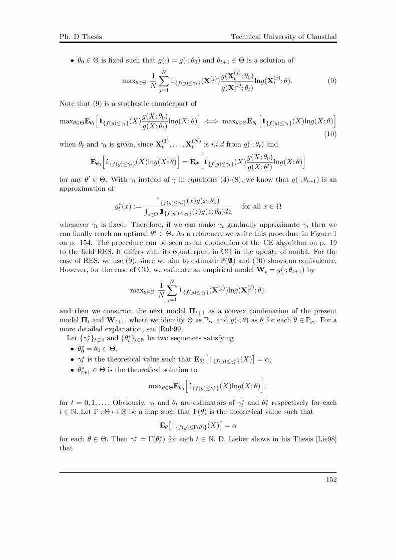
Ph. D Thesis Technical University of Clausthal
• θ0 ∈ Θ is fixed such that g(·) = g(·; θ0) and θt+1 ∈ Θ is a solution of
maxθ∈Θ1
N
N∑j=1
1f(y)≤γt(X(j))
g(X(j)t ; θ0)
g(X(j)t ; θt)
lng(X(j)t ; θ). (9)
Note that (9) is a stochastic counterpart of
maxθ∈ΘEθt
[1f(y)≤γt(X)
g(X; θ0)
g(X; θt)lng(X; θ)
]⇐⇒ maxθ∈ΘEθ0
[1f(y)≤γt(X)lng(X; θ)
](10)
when θt and γt is given, since X(1)t , . . . ,X
(N)t is i.i.d from g(·; θt) and
Eθ0
[1f(y)≤γt(X)lng(X; θ)
]= Eθ′
[1f(y)≤γt(X)
g(X; θ0)
g(X; θ′)lng(X; θ)
]for any θ′ ∈ Θ. With γt instead of γ in equations (4)-(8), we know that g(·; θt+1) is anapproximation of
g∗t (x) :=1f(y)≤γt(x)g(x; θ0)∫
z∈Ω 1f(y′)≤γt(z)g(z; θ0)dzfor all x ∈ Ω
whenever γt is fixed. Therefore, if we can make γt gradually approximate γ, then wecan finally reach an optimal θ∗ ∈ Θ. As a reference, we write this procedure in Figure 1on p. 154. The procedure can be seen as an application of the CE algorithm on p. 19to the field RES. It differs with its counterpart in CO in the update of model. For thecase of RES, we use (9), since we aim to estimate P(A) and (10) shows an equivalence.However, for the case of CO, we estimate an empirical model Wt = g(·; θt+1) by
maxθ∈Θ1
N
N∑j=1
1f(y)≤γt(X(j))lng(X
(j)t ; θ).
and then we construct the next model Πt+1 as a convex combination of the presentmodel Πt and Wt+1, where we identify Θ as Pce and g(·; θ) as θ for each θ ∈ Pce. For amore detailed explanation, see [Rub99].
Let γ∗t t∈N and θ∗t t∈N be two sequences satisfying
• θ∗0 = θ0 ∈ Θ,
• γ∗t is the theoretical value such that Eθ∗t
[1f(y)≤γ∗t (X)
]= α,
• θ∗t+1 ∈ Θ is the theoretical solution to
maxθ∈ΘEθ0
[1f(y)≤γ∗t (X)lng(X; θ)
],
for t = 0, 1, . . . . Obviously, γt and θt are estimators of γ∗t and θ∗t respectively for eacht ∈ N. Let Γ : Θ 7→ R be a map such that Γ(θ) is the theoretical value such that
Eθ
[1f(y)≤Γ(θ)(X)
]= α
for each θ ∈ Θ. Then γ∗t = Γ(θ∗t ) for each t ∈ N. D. Lieber shows in his Thesis [Lie98]that
152

Ph. D Thesis Technical University of Clausthal
Lemma 8.1 (see also Theorem 1.1 in [Rub99]). Assume that for each real number c ∈ R,there is a unique solution to
maxθ∈ΘEθ0
[1f(y)≤c(X)lng(X; θ)
],
and we use η(c) ∈ Θ to denote the unique solution (θ∗t+1 = η(γ∗t )). And suppose furtherthat
• γ∗t t∈N is monotonically increasing,
• the map Γ : Θ 7→ R is continuous,
• the map η : R 7→ Θ is proper, i.e. if c belongs to an interval, then η(c) belongs toa compact set,
• the map Γ(η(Γ(θ)
))− Γ(θ) is semi-continuous.
Then
limN→∞
P[γ0 > γ1 > γ2 > · · · > γt > · · ·
]= 1 and P
[∃t ∈ N, γt ≤ γ
]= 1.
Proof. see [Lie98].
Lemma 8.1 actually shows that under some ‘mild condition’, the procedure in Figure1 may stop with an optimal θ∗ ∈ Θ in finite many iterations if a suitable sample size isemployed.
153

Ph. D Thesis Technical University of Clausthal
Algorithm Cross entropy algorithm for rare event simulation
parameters:parametric family PIS = g(·; θ)|θ ∈ Θ, an α ∈ (0, 1) not very small, asample size N.
algorithm:
a) Generate random sample X(1)t , . . . ,X
(N)t i.i.d with g(·; θt), and or-
der them according to f as f(X(m1)t ) ≤ · · · ≤ f(X(mN )), set
γt = f(X(mbα·Nc)t );
b) Solve
maxθ∈Θ1
N
N∑j=1
1f(y)≤γt(X(j))
g(X(j)t ; θ0)
g(X(j)t ; θt)
lng(X(j)t ; θ)
and denote the solution as θt+1;
c) while (γt > γ)
c 1) t = t+ 1;
c 2) repeat step a)-c);
d) output θt;
Figure 1: Cross entropy algorithm for rare event simulation
154

Ph. D Thesis Technical University of Clausthal
A.7 Genetic algorithms, simulated annealing and particle swarmoptimization
A.7.1 Genetic algorithms
GAs are inspired by the natural evolution of genes of creatures. For a tutorial andoverview, see [Mic96] and [Whi94].
In GAs, problems are generally unconstrained 0-1 encoded. Therefore, we may assumean instance (S, f) here with S = 0, 1L for an L ∈ N.
Different from MBS, in GAs we call a collection of feasible solutions as a population.The input parameters for GAs are: a fixed parent population size N ∈ N, a fixedoffspring population size M ∈ N, a constant mutation rate rm ∈ (0, 1). The initialparent population P0 are uniformly sampled from S. And, in each sequent iteration t, afixed selection strategy is employed to choose M/2 pairs of solutions from Pt. After that,a crossover operator applies on each pair to produce two offspring, and each offspringmay encounter a mutation with probability rm. Here, we employ Ot to denote theresulted collection of offspring. Then, N many solutions in Ot ∪Pt would be selected toform Pt+1 by a fixed population update strategy.
In GAs, typical selection strategies are the roulette selection and tournament selection.In a roulette selection, we randomly pick out M many solutions from Pt by probabilitiesproportional to qualities of solutions. Then, the first pair is formed by the first andsecond selected solutions, the second pair is formed by the third and fourth selectedsolutions and so on. Tournament selection is similar with a real tournament competitionwith a fixed group size.
A crossover operator can be mathematically formulated as a random function whichtakes in two parents and outputs two children. Here, we take 1-point crossover as an ex-
ample. Given two solutions s(1) = (s(1)1 , s
(1)2 , . . . , s
(1)L ) and s(2) = (s
(2)1 , s
(2)2 , . . . , s
(2)L ), and
a randomly picked crossover point j from 1, . . . , L. Then 1-point crossover producestwo offspring as
o(1) = (s(1)1 , . . . , s
(1)j , s
(2)j+1, . . . , s
(2)L ) and o(2) = (s
(2)1 , . . . , s
(2)j , s
(1)j+1, . . . , s
(1)L ).
A typical mutation operator in GAs is the 1-flip. Given a solution (s1, . . . , sL) as wellas a random flip position i. Then 1-flip will mutate the solution into
(s1, . . . , si−1, 1− si, si+1, . . . , sL).
A population update strategy generally tells how to form the next parent populationfrom the current parent population and current offspring population. Typical updatestrategies may be the so-called λ+µ rule and (λ, µ) rule. In λ+µ rule, we will take thebest N many solutions in Pt∪Ot as the next population Pt+1. In (λ, µ) rule, Pt+1 wouldbe a random subsample from Ot with selection probabilities proportional to qualities ofqualities.
As a summary, we list the general GA algorithm in Figure 2 on p. 156.
155
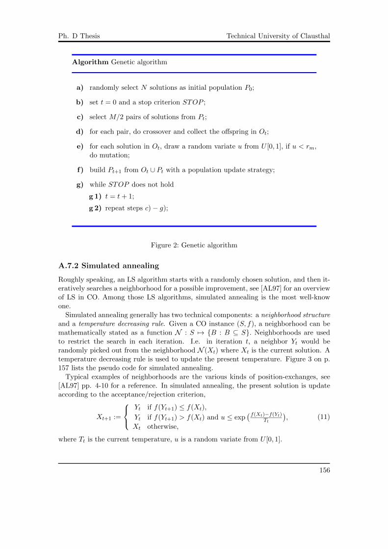
Ph. D Thesis Technical University of Clausthal
Algorithm Genetic algorithm
a) randomly select N solutions as initial population P0;
b) set t = 0 and a stop criterion STOP ;
c) select M/2 pairs of solutions from Pt;
d) for each pair, do crossover and collect the offspring in Ot;
e) for each solution in Ot, draw a random variate u from U [0, 1], if u < rm,do mutation;
f) build Pt+1 from Ot ∪ Pt with a population update strategy;
g) while STOP does not hold
g 1) t = t+ 1;
g 2) repeat steps c)− g);
Figure 2: Genetic algorithm
A.7.2 Simulated annealing
Roughly speaking, an LS algorithm starts with a randomly chosen solution, and then it-eratively searches a neighborhood for a possible improvement, see [AL97] for an overviewof LS in CO. Among those LS algorithms, simulated annealing is the most well-knowone.
Simulated annealing generally has two technical components: a neighborhood structureand a temperature decreasing rule. Given a CO instance (S, f), a neighborhood can bemathematically stated as a function N : S 7→ B : B ⊆ S. Neighborhoods are usedto restrict the search in each iteration. I.e. in iteration t, a neighbor Yt would berandomly picked out from the neighborhood N (Xt) where Xt is the current solution. Atemperature decreasing rule is used to update the present temperature. Figure 3 on p.157 lists the pseudo code for simulated annealing.
Typical examples of neighborhoods are the various kinds of position-exchanges, see[AL97] pp. 4-10 for a reference. In simulated annealing, the present solution is updateaccording to the acceptance/rejection criterion,
Xt+1 :=
Yt if f(Yt+1) ≤ f(Xt),
Yt if f(Yt+1) > f(Xt) and u ≤ exp(f(Xt)−f(Yt)
Tt
),
Xt otherwise,
(11)
where Tt is the current temperature, u is a random variate from U [0, 1].
156

Ph. D Thesis Technical University of Clausthal
Algorithm Simulated annealing
a) randomly choose an X0 from S, and fix an initial temperature T0;
b) set t = 0 and a stop criterion STOP ;
c) randomly choose an Yt from N (Xt);
d) choose Xt+1 from Xt, Yt according to (11);
e) update temperature;
f) while STOP does not hold
f 1) t = t+ 1;
f 2) repeat steps c)− f);
Figure 3: Simulated annealing
A.7.3 Particle swarm optimization
Particle swarm optimization (PSO, [KE95]) simulates the collective behavior of a schoolof fishes or birds. It generally assumes a continuous search space S. It employs a fixednumber of agents iteratively searching on S. Initially, the agents randomly construct astarting position (solution) on S. In each subsequent iteration, the agents move theirpresent positions towards their own best positions and the global best position. Theagents iteratively move their positions as following:
Initialization Randomly generate a swarm of positions of a fixed size N :
xi = (xi,1, . . . , xi,d) ∈ S, i = 1, . . . , N,
where d is the dimension. Initialize the N velocity vectors
v0i = (v0
i,1, . . . , v0i,d) ∈ Rd, i = 1, . . . , N.
Let bi denote the best position where agent i experienced, and b denote the globalbest position the swarm has ever visited so far. Take an inertia parameter e, andcognitive parameter c1 and a social parameter c2 from [0, 1].
Update Local and Global Information If it is the first iteration, then bi = xi and b isthe best position in the first swarm. Otherwise, if xi is better than bi, set bi = xi.And if b is worse than the best position in the current swarm, set b to be thatposition.
157

Ph. D Thesis Technical University of Clausthal
Update Velocity Generate two random numbers r1, r2 uniformly from [0, 1] and updatevelocities with the following form:
vt+1i = e · vt + r1 · c1 · (bi − xi) + r2 · c2 · (b− xi), (12)
for each i = 1, . . . , N.
Update Position Each position is updated by
xi = xi + vt+1i , (13)
for i = 1, . . . , N.
Although PSO is initially designed for continuous optimization, some recent literaturehave successfully applied it to combinatorial optimization, see e.g. [WHZP03]..
158
Bibliography
[AB09] Sanjeev Arora and Boaz Barak, Computational complexity: a modern ap-proach, Cambridge University Press, 2009.
[AEP05] N. Andreasson, A. Evggrafov, and M. Patriksson, An introduction tocontinuous optimization: Foundations and fundamental algorithms, Stu-dentlitteratur, 2005.
[AKRR05] G Alon, Dirk P Kroese, Tal Raviv, and Reuven Y Rubinstein, Appli-cation of the cross-entropy method to the buffer allocation problem in asimulation-based environment, Annals of Operations Research 134 (2005),no. 1, 137–151.
[AL97] EH Emile HL Aarts and Jan K Lenstra, Local search in combinatorialoptimization, Princeton University Press, 1997.
[Alp10] Ethem Alpaydin, Introduction to machine learning. 2nd, 2010.
[AM94] Hideki Asoh and Heinz Muhlenbein, On the mean convergence time ofevolutionary algorithms without selection and mutation, Parallel ProblemSolving from NaturePPSN III, Springer, 1994, pp. 88–97.
[Bal94] Shumeet Baluja, Population-based incremental learning. a method for inte-grating genetic search based function optimization and competitive learning,Tech. report, DTIC Document, 1994.
[BF03] S Ilker Birbil and Shu-Chering Fang, An electromagnetism-like mechanismfor global optimization, Journal of global optimization 25 (2003), no. 3,263–282.
[BHS97] Bernd Bullnheimer, Richard F Hartl, and Christine Strauss, A new rankbased version of the ant system. a computational study., SFB Adaptive In-formation Systems and Modelling in Economics and Management Science,WU Vienna University of Economics and Business, 1997.
[BHS99] , Applying the ant system to the vehicle routing problem, Meta-Heuristics, Springer, 1999, pp. 285–296.
[BR03] Christian Blum and Andrea Roli, Metaheuristics in combinatorial opti-mization: Overview and conceptual comparison, ACM Computing Surveys(CSUR) 35 (2003), no. 3, 268–308.
159
Ph. D Thesis Technical University of Clausthal
[BT93] Dimitris Bertsimas and John Tsitsiklis, Simulated annealing, StatisticalScience (1993), 10–15.
[CDMT94] Alberto Colorni, Marco Dorigo, Vittorio Maniezzo, and Marco Trubian,Ant system for job-shop scheduling, Belgian Journal of Operations Re-search, Statistics and Computer Science 34 (1994), no. 1, 39–53.
[CdVHM00] Oscar Cordon, Inaki Fernandez de Viana, Francisco Herrera, and LlanosMoreno, A new aco model integrating evolutionary computation concepts:The best-worst ant system, Citeseer, 2000.
[CHdM05] Krishna Chepuri and Tito Homem-de Mello, Solving the vehicle routingproblem with stochastic demands using the cross-entropy method, Annalsof Operations Research 134 (2005), no. 1, 153–181.
[Cin75] Erhan Cinlar, Introduction to stochastic processes, Printice-Hall, Engle-wood Cliffs, NJ, 1975.
[CJK07] Andre Costa, Owen Dafydd Jones, and Dirk Kroese, Convergence prop-erties of the cross-entropy method for discrete optimization, OperationsResearch Letters 35 (2007), no. 5, 573–580.
[CT12] Thomas M Cover and Joy A Thomas, Elements of information theory,John Wiley & Sons, 2012.
[CTCY10] Tianshi Chen, Ke Tang, Guoliang Chen, and Xin Yao, Analysis of compu-tational time of simple estimation of distribution algorithms, EvolutionaryComputation, IEEE Transactions on 14 (2010), no. 1, 1–22.
[DBIV+97] Jeremy S De Bonet, Ch L Isbell, Paul Viola, et al., Mimic: Finding op-tima by estimating probability densities, Advances in neural informationprocessing systems (1997), 424–430.
[DBKMR05] Pieter Tjerk De Boer, Dirk P Kroese, Shie Mannor, and Reuven Y Rubin-stein, A tutorial on the cross-entropy method, Annals of operations research134 (2005), no. 1, 19–67.
[DG97a] Marco Dorigo and Luca Maria Gambardella, Ant colonies for the travellingsalesman problem, BioSystems 43 (1997), no. 2, 73–81.
[DG97b] , Ant colony system: A cooperative learning approach to the travel-ing salesman problem, Evolutionary Computation, IEEE Transactions on1 (1997), no. 1, 53–66.
[DJ07] Benjamin Doerr and Daniel Johannsen, Refined runtime analysis of a ba-sic ant colony optimization algorithm., IEEE Congress on EvolutionaryComputation, 2007, pp. 501–507.
Bibliography 160

Ph. D Thesis Technical University of Clausthal
[DMC96] Marco Dorigo, Vittorio Maniezzo, and Alberto Colorni, Ant system: opti-mization by a colony of cooperating agents, Systems, Man, and Cybernet-ics, Part B: Cybernetics, IEEE Transactions on 26 (1996), no. 1, 29–41.
[DNSW07] Benjamin Doerr, Frank Neumann, Dirk Sudholt, and Carsten Witt, Onthe runtime analysis of the 1-ant aco algorithm, Proceedings of the 9thannual conference on Genetic and evolutionary computation, ACM, 2007,pp. 33–40.
[DS04] Marco Dorigo and Thomas Stutzle, Ant colony optimization, Cambridge,Massachusetts: A Bradford Book, MIT Press, 2004.
[DS10] , Ant colony optimization: overview and recent advances, Handbookof metaheuristics, Springer, 2010, pp. 227–263.
[Dur10] Rick Durrett, Probability: theory and examples, vol. 3, Cambridge univer-sity press, 2010.
[GD+95] Luca Maria Gambardella, Marco Dorigo, et al., Ant-q: A reinforcementlearning approach to the traveling salesman problem, ICML, 1995, pp. 252–260.
[GL95] M Grotschel and L Lovasz, Combinatorial optimization, Handbook of com-binatorics 2 (1995), 1541–1597.
[GL99] Fred Glover and Manuel Laguna, Tabu search, Springer, 1999.
[GM02] Michael Guntsch and Martin Middendorf, A population based approach foraco, Applications of Evolutionary Computing, Springer, 2002, pp. 72–81.
[Gou06] Nicholas Gould, An introduction to algorithms for continuous optimization,Oxford University Computing Laboratory Notes, 2006.
[Gut00] Walter J Gutjahr, A graph-based ant system and its convergence, FutureGeneration Computer Systems 16 (2000), no. 8, 873–888.
[Gut02] , Aco algorithms with guaranteed convergence to the optimal solu-tion, Information processing letters 82 (2002), no. 3, 145–153.
[Gut03] , A generalized convergence result for the graph-based ant systemmetaheuristic, Probability in the Engineering and Informational Sciences17 (2003), no. 4, 545–569.
[Gut07] , Mathematical runtime analysis of aco algorithms: Survey on anemerging issue, Swarm Intelligence 1 (2007), no. 1, 59–79.
[Gut08] , First steps to the runtime complexity analysis of ant colony opti-mization, Computers & Operations Research 35 (2008), no. 9, 2711–2727.
Bibliography 161

Ph. D Thesis Technical University of Clausthal
[HGC95] David Heckerman, Dan Geiger, and David M Chickering, Learningbayesian networks: The combination of knowledge and statistical data, Ma-chine learning 20 (1995), no. 3, 197–243.
[HLG99] Georges R Harik, Fernando G Lobo, and David E Goldberg, The compactgenetic algorithm, Evolutionary Computation, IEEE Transactions on 3(1999), no. 4, 287–297.
[HP11] Mark Hauschild and Martin Pelikan, An introduction and survey of esti-mation of distribution algorithms, Swarm and Evolutionary Computation1 (2011), no. 3, 111–128.
[Jen06] Johan Ludwig William Valdemar Jensen, Sur les fonctions convexes et lesinegalites entre les valeurs moyennes, Acta Mathematica 30 (1906), no. 1,175–193.
[KE95] J Kennedy and R Eberhart, Particle swarm optimization, Neural Net-works, 1995. Proceedings., IEEE International Conference on, vol. 4, IEEE,1995, pp. 1942–1948.
[KGOK12] Dervis Karaboga, Beyza Gorkemli, Celal Ozturk, and Nurhan Karaboga,A comprehensive survey: artificial bee colony (abc) algorithm and applica-tions, Artificial Intelligence Review (2012), 1–37.
[Kno90] K. Knopp, Theory and application of infinite series, Courier Dover Pub-lisher, 1990.
[KV02] Bernhard Korte and Jens Vygen, Combinatorial optimization: theory andalgorithms, second ed., Springer, 2002.
[Law01] Eugene L Lawler, Combinatorial optimization: networks and matroids,DoverPublications. com, 2001.
[LDM09] Manuel Laguna, Abraham Duarte, and Rafael Marti+1, Hybridizing thecross-entropy method: An application to the max-cut problem, Computers& Operations Research 36 (2009), no. 2, 487–498.
[Lie98] D. Lieber, Rare events estimation via cross entropy and importance sam-pling, William Davidson Faculty of Industrial Engineering and Manage-ment, Technion, Haifa, Israel, 1998.
[Mar05] Leonid Margolin, On the convergence of the cross-entropy method, Annalsof Operations Research 134 (2005), no. 1, 201–214.
[Mic96] Zbigniew Michalewicz, Genetic algorithms+ data structures= evolutionprograms, springer, 1996.
Bibliography 162

Ph. D Thesis Technical University of Clausthal
[ML09] Tai-Yu Ma and Jean-Patrick Lebacque, A cross entropy based multi-agentapproach to traffic assignment problems, Traffic and Granular Flow07,Springer, 2009, pp. 161–170.
[MMR99] Heinz Muhlenbein, Thilo Mahnig, and Alberto Ochoa Rodriguez,Schemata, distributions and graphical models in evolutionary optimization,Journal of Heuristics 5 (1999), no. 2, 215–247.
[MP96] H Muhlenbein and G Paaß, From recombination of genes to the estima-tion of distributions i. binary parameters, Parallel Problem Solving fromNaturePPSN IV, Springer, 1996, pp. 178–187.
[Nic07] TAJ Nicholson, Optimization in industry: Optimization techniques, vol. 1,Transaction Publishers, 2007.
[NW06] Frank Neumann and Carsten Witt, Runtime analysis of a simple ant colonyoptimization algorithm, Springer, 2006.
[NW09] , Runtime analysis of a simple ant colony optimization algorithm,Algorithmica 54 (2009), no. 2, 243–255.
[OHS+11] S. M. Oliveira, M. S. Hussin, T. Stuetzle, A. Roli, and M. Dorigo, A detailedanalysis of the population-based ant colony optimization algorithm for thetsp and the qap, GECCO’11 Proceedings of the 13th annual conferencecompanion on the Genetic and evolutionary computation (New York, NY,USA), 2011, pp. 13–14.
[Pel05] Martin Pelikan, Bayesian optimization algorithm, Hierarchical BayesianOptimization Algorithm, Springer, 2005, pp. 31–48.
[PGCP00] Martin Pelikan, David E Goldberg, and Erick Cantu-Paz, Linkage problem,distribution estimation, and bayesian networks, Evolutionary computation8 (2000), no. 3, 311–340.
[PGL02] Martin Pelikan, David E Goldberg, and Fernando G Lobo, A survey ofoptimization by building and using probabilistic models, Computational op-timization and applications 21 (2002), no. 1, 5–20.
[PM98] Martin Pelikan and Heinz Muhlenbein, Marginal distributions in evolution-ary algorithms, Proceedings of the International Conference on GeneticAlgorithms Mendel, vol. 98, Citeseer, 1998, pp. 90–95.
[RK04] Reuven Y Rubinstein and Dirk P Kroese, The cross-entropy method: a uni-fied approach to combinatorial optimization, monte-carlo simulation andmachine learning, Springer, 2004.
[RP95] Motwani Rajeevi and Raghavan Prabhakar, Randomized algorithms, Cam-bridge University Press, 1995.
Bibliography 163

Ph. D Thesis Technical University of Clausthal
[RT+09] Gerardo Rubino, Bruno Tuffin, et al., Rare event simulation using montecarlo methods, Wiley Online Library, 2009.
[Rub97] Reuven Y Rubinstein, Optimization of computer simulation models withrare events, European Journal of Operational Research 99 (1997), no. 1,89–112.
[Rub99] , The cross-entropy method for combinatorial and continuous op-timization, Methodology and computing in applied probability 1 (1999),no. 2, 127–190.
[Rub02] , Cross-entropy and rare events for maximal cut and partitionproblems, ACM Transactions on Modeling and Computer Simulation(TOMACS) 12 (2002), no. 1, 27–53.
[SBW11] Budi Santosa, Muhammad Arif Budiman, and Stefanus Eko Wiratno, Across entropy-genetic algorithm for m-machines no-wait job-shop schedul-ing problem, Journal of Intelligent Learning Systems and Applications 3(2011), 171–180.
[SG00] Kumara Sastry and David E Goldberg, On extended compact genetic algo-rithm, Late-Breaking Paper at the Genetic and Evolutionary ComputationConference, 2000, pp. 352–359.
[SH00] Thomas Stutzle and Holger H Hoos, Max–min ant system, Future genera-tion computer systems 16 (2000), no. 8, 889–914.
[SVVdW80] Edward A Silver, R Victor, V Vidal, and Dominique de Werra, A tutorialon heuristic methods, European Journal of Operational Research 5 (1980),no. 3, 153–162.
[Tra84] Boris A Trakhtenbrot, A survey of russian approaches to perebor (brute-force searches) algorithms, Annals of the History of Computing 6 (1984),no. 4, 384–400.
[Whi94] Darrell Whitley, A genetic algorithm tutorial, Statistics and computing 4(1994), no. 2, 65–85.
[WHZP03] Kang-Ping Wang, Lan Huang, Chun-Guang Zhou, and Wei Pang, Parti-cle swarm optimization for traveling salesman problem, Machine Learningand Cybernetics, 2003 International Conference on, vol. 3, IEEE, 2003,pp. 1583–1585.
[WK14a] Zijun Wu and Michael Kolonko, Absorption in model-based search algo-rithms for combinatorial optimization, Evolutionary Computation (CEC),2014 IEEE Congress on, IEEE, 2014, pp. 1744–1751.
Bibliography 164

Ph. D Thesis Technical University of Clausthal
[WK14b] , Asymptotic properties of a generalized cross entropy optimizationalgorithm, Evolutionary Computation, IEEE Transactions on 18 (2014),no. 5, 658–673.
[WM97] David H Wolpert and William G Macready, No free lunch theorems foroptimization, Evolutionary Computation, IEEE Transactions on 1 (1997),no. 1, 67–82.
[Woe03] Gerhard J Woeginger, Exact algorithms for np-hard problems: A survey,Combinatorial OptimizationEureka, You Shrink!, Springer, 2003, pp. 185–207.
[WS11] David P Williamson and David B Shmoys, The design of approximationalgorithms, Cambridge University Press, 2011.
[ZBMD04] Mark Zlochin, Mauro Birattari, Nicolas Meuleau, and Marco Dorigo,Model-based search for combinatorial optimization: A critical survey, An-nals of Operations Research 131 (2004), no. 1-4, 373–395.
[ZM04] Qingfu Zhang and Heinz Muhlenbein, On the convergence of a class ofestimation of distribution algorithms, Evolutionary Computation, IEEETransactions on 8 (2004), no. 2, 127–136.
Bibliography 165

Index
σ-algebra, 145∼ notation, 148
algorithm, 10
big Ω, 148big Θ, 148Borel space, 145bounded above (big O), 148
change of measure, 150combinatorial optimization, 6–9
elements, 6–7feasible set, 6feasible solution, 6instance, 6maximizing instance, 6maximizing problem, 8minimizing instance, 6minimizing problem, 8objective, 7objective function, 6objective value, 6optimal solution, 6optimum, 7problem, 8
examples, 8–9AP, 9KP, 9MaxCut, 9TSP, 8
conditional entropy, 143conditional probability, 145constant learning rate, 63cut, 9cutting benefit, 9
expectation, 147exponential runtime, 69
feasible under feasibility distributions, 75
genetic drift, 100graph, 141
branch, 142circuit or circle, 141connected graph, 142directed graph, 141forest, 142fully or completely connected, 142Hamiltonian circle, 141leaf, 142path, 141root, 142spanning graph, 141subgraph, 141tree, 142undirected graph, 141walk, 141weighted graph, 142
Heuristic search, 10–12
Kullback-Leibler, 143Kullback-Leibler (K-L) distance or di-
vergence, 150
linear programming, 47linear programming
integer programming, 144linear program, 144zero-one integer programming, 144
linear programming optimization, 144
166

Ph. D Thesis Technical University of Clausthal
Markov chain, 147measurable function, 146measurable set, 145measurable space, 145model mutation, 42model-based search, 11, 13–66
a unified model family, 50absorbing solution, 98absorption of models, 98absorption of solutions, 98alphabet, 46ant colony optimization, 23–32
ant cycle, 24archive, 31assessment function, 27choice probability, 28construction graph, 25evaporation rate, 27feasible continuation, 26global evaporation rate, 31global update, 31legal walk, 26local evaporation rate, 31local update, 30model family, 30out rule, 32partial legal walk, 26pheromones, 23pheromones matrix, 30pseudo random proportional rule,
30visibility, 29
basic recursion, 58basic requirement, 14compatible to feasibility distributions,
75compatible to optimal solution, 70concatenation, 47concentrated solution, 98constrained instance, 46constraints, 49cross entropy algorithm, 16–21
model family, 17parameters, 18
penalty objective value, 16smooth parameter, 18variants, 20
empty string, 47estimation of distribution algorithms,
37–44choice rule, 40learning rate, 42memory, 40memory update rule, 40model family, 37model mutation, 42random shift, 43
extension, 47feasibility distribution, 51finite reachability, 69framework , 57–58global truncate memory update, 59greedy feasibility construction, 51identity selection, 60initial model, 14leading partial solution, 65leading string, 47length of a string, 47limit of the models, 98local truncate memory update, 59Markov property, 66memory identity selection, 60memory random selection, 60motivation, 14–15multivariate marginal models, 13non-greedy feasibility distribution or
construction, 51non-memory update, 59problem size, 69random selection, 60relative efficiency, 138runtime, 69search capacity, 133single-start local search, 15solutions’ length, 46string encoding or representation, 46tail property, 107
Index 167

Ph. D Thesis Technical University of Clausthal
time dependent weighted learning,61
truncate selection, 60unconstrained instance, 46underlying stochastic process, 64uniform learning, 60univariate marginal models, 13weighted learning, 61
mutual information, 143
outcome, 145
probabilistic independence, 145
random event, 145random variable, 146
sample space, 145Shannon entropy, 143small ω, 148small o, 148solutions-based search, 11stagnation, 100state space, 146stochastic process, 147strategy, 63surrogate probability, 75
total cost, 9total entropy, 143traveling cost, 8
variance minimization, 150
worst out, 59
zero variance change of measure, 150
Index 168