model-based extraction of femoral medulla ducts from radiographic images

Model-based extraction of femoral medulla ducts

from radiographic images

Franco Bartolinia,†, Monica Carfagnib, Lapo Governib,*

aDipartimento di Elettronica e Telecomunicazioni, Universita di Firenze, Via Santa Marta 3, Firenze 50139, ItalybDipartimento di Meccanica e Tecnologie Industriali, Universita di Firenze, Via Santa Marta 3, Firenze 50139, Italy

Received 25 June 2002; received in revised form 3 June 2003; accepted 12 June 2003

Abstract

The planning of the hip prosthesis surgical operation is usually performed manually by the surgeon, who ‘draws’ on a patient’s X-ray

image the outline of the prosthetic stem in order to choose the one most suitable for the case at hand. In an attempt to give some repeatability

and objectivity to the planning phase, a procedure has been devised for hip prosthesis’ stem selection based on the extraction of the femoral

relevant outlines.

This work presents a computer aided method aimed at automatically extracting the medulla duct outlines from a human femur radiographic

image. The outlines are retrieved by referring to a suitable geometric model of the generic femoral cross-section; the projection function

obtained by simulating the radiographic acquisition of such a model is fitted on the grey-level functions corresponding to the rows of the

actual digitised radiographic image by means of a least squares algorithm. The resulting outlines are used in a software tool performing the

hip prosthesis pre-operational planning.

q 2003 Published by Elsevier B.V.

Keywords: Model-based image processing; Medical images processing; Surgery aiding tools

1. Introduction

The Total Hip Replacement pre-operational planning is a

procedure meant to help surgeons to choose the proper

prosthesis for a given patient. The pre-operational planning

is usually carried out by using templates provided by hip

prostheses manufacturers. Such templates contain the

profiles of each different prosthesis model available for

the surgical operation. The surgeon superimposes each

template on a radiographic image of the coxo-femoral

region of the patient, manually trying to match the

prosthesis profile with the patient bone anatomy. Once a

suitable template is found, the corresponding prosthesis is

chosen to be implanted. It is obvious that such a procedure is

highly subjective and its results, consequently, may vary

depending on the surgeon performing the planning.

For this reason a system [1] has been previously

developed capable of performing part of the planning in a

completely automatic way. The system is based on the

estimation of the femoral geometry performed through the

extraction, from a digitised X-ray tomography of the patient

(Fig. 1), of the contours of the medulla duct’s and of the

femoral outlines.

Unfortunately X-ray tomographic machines are not often

found in hospital equipment, while radiographic devices are

widely available. Consequently, the applicability of the

system to conventional radiographic images was tested. In

Fig. 2 the poor performance of an edge extraction procedure

applied to a conventional radiographic image, is shown,

compared with the results obtained from the application of

the same procedure to a tomographic image (in both cases a

classical Laplacian of Gaussian—LoG—edge detector with

standard deviation of 3.5 is used). Such behavior can be

explained by considering the different method used by,

respectively, the tomographic and the radiographic

machines to generate the images. The first type of

techniques makes use of the relative motion between the

0262-8856/$ - see front matter q 2003 Published by Elsevier B.V.

doi:10.1016/S0262-8856(03)00118-5

Image and Vision Computing 22 (2004) 173–182

www.elsevier.com/locate/imavis

† In memory of Franco, Friend and Colleague, whose untimely on

January 1st, 2004 passing occurred* Corresponding author. Tel.: þ39-55-479-6509; fax: þ39-55-479-6394.

E-mail address: [email protected] (L. Governi).

http://www.elsevier.com/locate/imavis

patient and the X-ray source to focus a desired plane of

interest in the patient’s anatomy, hiding all the structures

that lie, along the optical axis, above or behind that plane;

while the second type of techniques produces a simple

projection of all the anatomic structures located between the

X-ray source and the image support, thereby overlapping

different anatomic regions. As a matter of fact, usual edge

detection techniques, that detect the loci of maxima of the

image gradient (or of the zeros of second order derivative)

demonstrated not to be a good choice for this problem, given

that such loci do not have, in the case of radiographic images,

a real physical correspondent. This is better exemplified in

Fig. 3, where the step edge profile (that corresponds to the

model of contours detected by the common derivative-based

Fig. 1. Contour extraction and prosthesis choice performed by the software for pre-operation planning.

Fig. 2. Edges extracted from the radiographic image (left) compared to those extracted from the X-ray tomographic image (right).

Fig. 3. Comparison between the step edge profile (left) representing the

model of contour profile assumed by common derivative-based edge

detector (e.g. LoG), and the edge profile (right) that is the suitable model for

the contour of the medulla duct internal outline.

F. Bartolini et al. / Image and Vision Computing 22 (2004) 173–182174

edge detectors) is compared to the contour profile that is

found in radiographic images in correspondence to the

medulla duct internal outline.

Accordingly conventional image processing techniques

[2–4] proved to be not effective. On the other hand,

several studies demonstrated the effectiveness of active

contours, known as snakes curves, in detecting continu-

ous outlines in X-ray images [5,6]. This approach,

however, has the drawback of requiring an accurate

tuning of the coefficients in the mathematical formulation

of the active contour itself in order to obtain robust

results; moreover it generally does not take into account

a priori knowledge on the 3D geometry of the object to

be analysed (in our case the bone). In order to bypass

this drawback, a new methodology for femoral contours

extraction was developed, that explicitly take into

account the characteristics of the process of image

formation.

2. The femoral cross-section model

The considerations drawn in the previous paragraph lead

us to develop a new methodology strictly related to the

specific kind of images we have to work on. The basic idea

of the new approach is to employ a geometrical parametric

model of the generic cross-section of the human femur. By

using such a model it is possible to anticipate the trend of the

grey-level function exhibited by radiographic images. The

use of a model will also contribute to avoid the image noise

to mislead the contour extraction process. Let us now see the

details of the model development.

First of all many different images of the human femur’s

cross-sections (Fig. 4) were examined. For this purpose the

Visible Human Project database (URL: http://www.nlm.nih.

gov/research/visible/) was used. At a first glance, we

assumed it was possible to model the femur’s cross-section

by an annular hoop, parameterised by the x co-ordinates of

the two circumferences centres—C and c—and by the two

radii—R and r—(Fig. 5).

By considering that a radiography basically measures the

transparency of human body matter went through by X-rays

along directions of projection orthogonal to the radiographic

plane, and by assuming that the transparency of the medulla

Fig. 4. An image of a femoral cross-section taken from the Visible Human

Project database.

Fig. 5. The annular hoop model.

Fig. 6. Projection function obtained by subtracting the two circumferences.

In the figure it is assumed that C ; c:

F. Bartolini et al. / Image and Vision Computing 22 (2004) 173–182 175

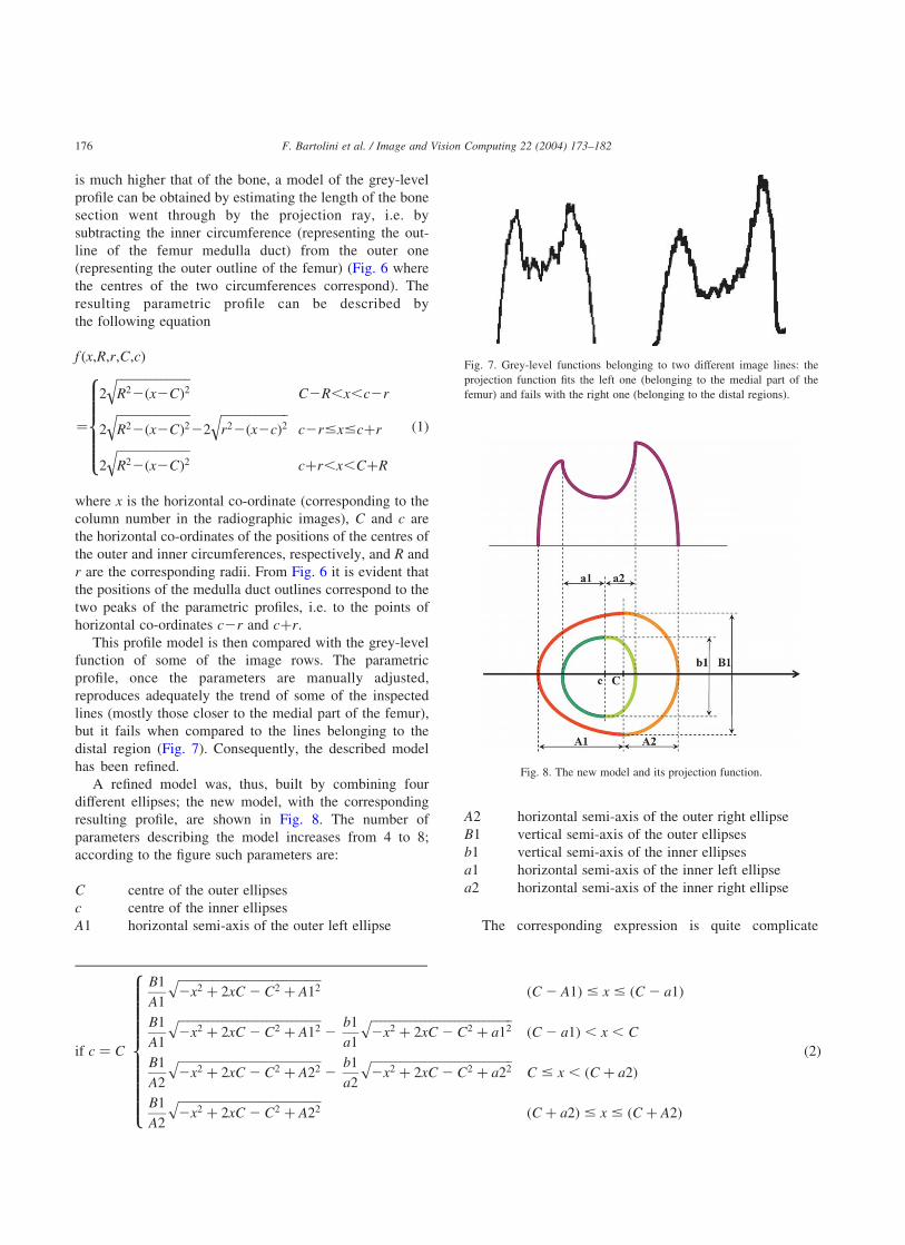
http://www.nlm.nih.gov/research/visible/

http://www.nlm.nih.gov/research/visible/

is much higher that of the bone, a model of the grey-level

profile can be obtained by estimating the length of the bone

section went through by the projection ray, i.e. by

subtracting the inner circumference (representing the out-

line of the femur medulla duct) from the outer one

(representing the outer outline of the femur) (Fig. 6 where

the centres of the two circumferences correspond). The

resulting parametric profile can be described by

the following equation

f ðx;R;r;C;cÞ

¼

2

ffiffiffiffiffiffiffiffiffiffiffiffiffiffiffiR22ðx2CÞ2

qC2R,x,c2r

2


q22

ffiffiffiffiffiffiffiffiffiffiffiffiffiffir22ðx2cÞ2

qc2r#x#cþr

2


qcþr,x,CþR

8>>>>><>>>>>:

ð1Þ

where x is the horizontal co-ordinate (corresponding to the

column number in the radiographic images), C and c are

the horizontal co-ordinates of the positions of the centres of

the outer and inner circumferences, respectively, and R and

r are the corresponding radii. From Fig. 6 it is evident that

the positions of the medulla duct outlines correspond to the

two peaks of the parametric profiles, i.e. to the points of

horizontal co-ordinates c2r and cþr:

This profile model is then compared with the grey-level

function of some of the image rows. The parametric

profile, once the parameters are manually adjusted,

reproduces adequately the trend of some of the inspected

lines (mostly those closer to the medial part of the femur),

but it fails when compared to the lines belonging to the

distal region (Fig. 7). Consequently, the described model

has been refined.

A refined model was, thus, built by combining four

different ellipses; the new model, with the corresponding

resulting profile, are shown in Fig. 8. The number of

parameters describing the model increases from 4 to 8;

according to the figure such parameters are:

C centre of the outer ellipses

c centre of the inner ellipses

A1 horizontal semi-axis of the outer left ellipse

A2 horizontal semi-axis of the outer right ellipse

B1 vertical semi-axis of the outer ellipses

b1 vertical semi-axis of the inner ellipses

a1 horizontal semi-axis of the inner left ellipse

a2 horizontal semi-axis of the inner right ellipse

The corresponding expression is quite complicate

if c ¼ C

B1

A1

ffiffiffiffiffiffiffiffiffiffiffiffiffiffiffiffiffiffiffiffiffiffiffiffiffiffiffiffiffi2x2 þ 2xC 2 C2 þ A12

pðC 2 A1Þ # x # ðC 2 a1Þ

B1

A1


p2

b1

a1

ffiffiffiffiffiffiffiffiffiffiffiffiffiffiffiffiffiffiffiffiffiffiffiffiffiffiffiffiffi2x2 þ 2xC 2 C2 þ a12

pðC 2 a1Þ , x , C

B1

A2


p2

b1

a2

ffiffiffiffiffiffiffiffiffiffiffiffiffiffiffiffiffiffiffiffiffiffiffiffiffiffiffiffiffi2x2 þ 2xC 2 C2 þ a22

pC # x , ðC þ a2Þ

B1

A2


pðC þ a2Þ # x # ðC þ A2Þ

8>>>>>>>>>>><>>>>>>>>>>>:

ð2Þ

Fig. 7. Grey-level functions belonging to two different image lines: the

projection function fits the left one (belonging to the medial part of the

femur) and fails with the right one (belonging to the distal regions).

Fig. 8. The new model and its projection function.


since many different cases must be pointed out as shown

in the following equations:

if c , C

ffiffiffiffiffiffiffiffiffiffiffiffiffiffiffiffiffiffiffiffiffiffiffiffiffiffiffiffiffiffiffiffiffiffi2x2 þ 2xC 2 C2 þ A12

B1

A1

rðC 2 A1Þ # x # ðc2 a1Þ


B1

A1

r2

ffiffiffiffiffiffiffiffiffiffiffiffiffiffiffiffiffiffiffiffiffiffiffiffiffiffiffiffiffiffiffiffi2x2 þ 2xc2 c2 þ a12

b1

a1

rðc2 a1Þ , x , c


B1

A1

r2


b1

a2

rc # x # C


B1

A2

r2


b1

a2

rC , x , ðcþ a2Þ


B1

A2

rðcþ a2Þ # x # ðC þ A2Þ

8>>>>>>>>>>>>>>>>><>>>>>>>>>>>>>>>>>:

ð3Þ

if c . C


B1

A1

rðC 2 A1Þ # x # ðc2 a1Þ


B1

A1

r2


b1

a1

rðc2 a1Þ , x , C


B1

A2

r2


b1

a1

rC # x # c


B1

A2

r2


b1

a2

rc , x , ðcþ a2Þ


B1

A2

rðcþ a2Þ # x # ðC þ A2Þ

8>>>>>>>>>>>>>>>>><>>>>>>>>>>>>>>>>>:

ð4Þ

Adjusting the parameters values it is now possible to fit

the grey-level function of any image row crossing the femur

(Fig. 9).

The refined models can then be fitted according to a least

squares [7] criterion to every row of the radiographic image

in such a way to identify, for each row, the horizontal co-

ordinates of the medulla duct outlines. The details of the

actual fitting procedure are given in next section.

3. The contour extraction procedure

On the basis of the described model of the femur’s cross-

section, a procedure to automatically retrieve the medulla

duct outlines has been developed. The basic steps may be

summarised as follows:

1. Definition of an user selected guiding outline.

2. Definition of an area of interest (AoI) on the basis of the

guiding outline.

3. Detection of auxiliary external outlines.

4. Extraction of the femoral medulla duct’s outlines (i.e.

the desired outlines).

A detailed description of all these steps follows in next

subsections.

3.1. The guiding outline

The guiding outline is a user defined curve, created by

picking some desired points on the image by means of the

mouse. At the beginning of the procedure the user is

asked to draw a rough profile approximating the femur’s

external outline. This task is accomplished by selecting

the nodes of two poly-lines approximating, respectively,

the right and left external femoral contours (Fig. 10, left).

After the nodes have been selected, the resulting poly-

lines are converted into two spline curves, of degree 5,

interpolating the nodes; these curves will be called from

now on guiding outline. Such user defined outline was

used, in a previous work to allow the computation of the

direction perpendicular to the edges to be extracted [1],

but in this work it has been introduced for a completely

different reason. In the following subsection its purpose

will be explained.

3.2. The area of interest

The first reason to introduce the guiding outline is to


identify an AoI on the original image. The AoI is delimited

by the highest and the lowest horizontal segments joining

both the left and right part of the guiding outline and by the

guiding outline itself (Fig. 10, right). In this way the medulla

duct contour to be retrieved is entirely contained in the AoI,

and, consequently, the size of the image portion to be

processed is considerably reduced.

3.3. The auxiliary external outlines

Once the portion of the image to be processed has

been reduced through the definition of the AoI, a least

square best fitting procedure is repeated for each row in

order to automatically determine the proper parameters to

approximate the grey-level row profile. As already

Fig. 9. Two sample image rows fitted with the new projection function.


mentioned, the basic idea is to use the obtained best

fitting parametric profile to determine the two relative

maximum points and, consequently, the location of the

medulla duct edges for that image row (Fig. 11).

Unfortunately this objective can be reached only if the

parameters starting values are close enough to the

optimal ones. This fact is due to the large number of

parameters to be simultaneously optimised, and to the

non-linear nature of the best fitting problem at hand.

Consequently it is necessary to devise a method to cope

with this problem. This has been done by developing a

procedure capable of firstly detecting the external femoral

outlines.

The external femoral outlines provide a very useful tool

for reducing the number of parameters involved in the

search for the best fitting projection function: in fact, for

each image row, the external outlines have the same

position of the two most external points of the correspond-

ing cross-section model. Once such points are known, three

out of the eight parameters determining the projection

function are not independent any more. In particular, by

naming xL and xR; respectively, the left and right co-

ordinates of the so determined external outlines, it results

that C ¼ xL þ A1; and A2¼ xR 2 xL 2A1: Consequently,

the least squares minimisation, needed to identify the best

fitting profile, has to estimate only six of the eight initial

parameters. This reduction proved to be very effective in

decreasing the minimisation procedure sensitivity to the

starting parameters values.

The procedure for detecting the external outlines,

which is applied to all the rows of the image, is based,

in its turn, on a least squares minimisation algorithm.

First, a tolerance range is automatically defined by a

width depending on the images resolution, across the

guiding outline (here it is the second reason for the

guiding outline to be introduced), and only in such a

range the external outlines is actually looked for (Fig. 12,

Fig. 10. The user defined poly-line approximating the femoral external

outlines (left) and the resulting area of interest (right).

Fig. 11. The medulla duct’s outlines for a given line correspond to the local

maxima of the best fitting projection function.

Fig. 12. The automatically defined tolerance range across the guide outline (left), and a portion of the projection function used to fit a desired row segment (right).


left), then the projection of a portion of the cross-section

model is fitted on the row segment delimited by the

tolerance range (Fig. 12, right). The considered projection

function portions are constituted by the left and right

external ellipses, respectively, for the left and right

external outline; consequently the parameters required to

define them are only the centre of the outer ellipses C; the

vertical semi-axis B1 and one of the horizontal semi-axis

A1 or A2: Using such a number of parameters the best

fitting function for each line is easily found out, therefore

allowing the location of the external outline. The

extraction of the external femoral outline is only

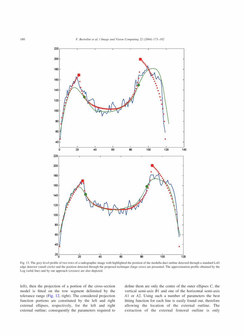
Fig. 13. The grey-level profile of two rows of a radiographic image with highlighted the position of the medulla duct outline detected through a standard LoG

edge detector (small circle) and the position detected through the proposed technique (large cross) are presented. The approximation profile obtained by the

Log (solid line) and by our approach (crosses) are also depicted.


dependent on the location of the tolerance range (Fig. 12,

left): while we are proposing to define this range by

identifying a guiding outline, alternative approaches are

feasible, as for example the definition of a strip where

the actual position of the femoral external outline is

known to be included.

3.4. The actual extraction of the medulla duct outlines

Once the external outlines are located it is a relatively

easy task to extract the medulla duct outlines.

† Starting from the lowest image row in the AoI a least

square minimisation algorithm is applied, using default

starting values for the six required parameters. These

default values are chosen based on the guiding outline;

more in particular it is assumed, for the first image row,

that the femoral cross-section can be represented by a

perfect annular hoop with the inner circle having a radius

equal to 45% of the outer one (the outer circle radius is

provided by the guiding outline).

† The corresponding best fitting profile is thereby com-

puted and the edge (maxima) points are located.

† The following image row is selected (according to a

user defined step index) and the least square estimation

performed again. The initial values for the parameters

are determined on the basis of both the optimised

values deriving from the previous line and the trend of

the external outline enclosed between the current row

and the previous one.

† This last step is iterated for each desired row belonging

to the AoI so that the complete medulla duct outline is

retrieved.

4. Results

The described procedure has been applied to several

test X-ray images, in order to evaluate its performance in

terms of repeatability and robustness; the sensitivity to

the user’s errors in selecting the guiding outline has been

also tested. In this section some selected results are

presented.

First of all to prove the major effectiveness of the

model-based approach with respect to standard edge

extraction techniques for the problem at hand, in Fig. 13

the grey-level profiles of two rows of a radiographic

image are depicted. The position of the medulla duct

outline detected by the proposed technique is highlighted

with a large cross, while the position detected by means

of a classical LoG edge detector with standard deviation

of 3.5 is highlighted with a small circle. The approxi-

mation profiles obtained by the two methods are also

plotted (with a solid line the profile approximated by the

LoG, and with crosses the profile approximated through

our model-based approach). It is evident that the precision

of the proposed approach is much higher. In fact, given

the profile of the projection function, the position

identified by the LoG, i.e. the point of zero second

Fig. 14. The effects of inaccurate user selected guiding outline and (centre and right) of poorly contrasted image (left) are presented. The medulla duct outline is

always well detected.


order derivative, has almost nothing to do with the edge

of the medulla duct outline.

In Fig. 14 the effects of inaccurate user selected guiding

outlines and of differently contrasted images are shown: it is

evident that the proposed method is strongly insensitive

both to the very inaccurate initial manual selection of the

guiding outline and to the variations of dynamic range of the

images to be processed. A similar insensitivity is exhibited

by the proposed approach with respect to the number of

points used for defining the guiding outlines.

For comparison the results obtained by a previous

method [1] relying on a standard LoG operator are shown

in Fig. 15. Anyway it is important to stress again that the use

of LoG operator can be source of a systematic error, given

that it detects the points of the profile where second order

derivatives become null, but, because of the particular

formation process of radiographic images, these do not have

any physical meaning. On the contrary the maxima of the

profile estimated by the proposed model-based approach

correspond to the location of the femur medulla duct.

5. Conclusions

In this paper a novel approach has been presented for

extracting the femoral medulla duct outlines from radio-

graphic images. The effectiveness of the approach is based

on the use of a model of the femoral cross-section and on

the simulation of the radiographic projection process, to

build up a parametric grey-level profile which is fitted to

the pixels values extracted from the rows of the radio-

graphic images. The approach has proved to be very

robust, repeatable and immune to user errors. The

implemented procedure has been included in the pre-

operational system described in Ref. [1], thus enabling

processing of both X-ray tomographic and conventional

radiographic images.

Future work will be addressed to retrieve the geometry of

mutually orthogonal femoral cross-sections, by applying the

procedure to two distinct radiographic images (frontal and

lateral views). Once both the axes are computed it will be

possible to perform a complete reconstruction of the entire

3D femoral geometry at an extremely low cost.

Acknowledgements

The authors would like to thank Francesco Crispini for

the help provided in implementing the system.

References

[1] D. Bongini, M. Carfagni, L. Governi, Hippin: a semiautomatic

computer program for selecting hip prosthesis femoral components,

Computer Methods and Programs in Biomedicine 63 (2000)

105–115.

[2] R.C. Gonzales, R.E. Woods, Digital Image Processing, Addison-

Wesley, New York, 1992.

[3] J.C. Russ, The Image Processing Handbook, CRC Press, Boca Raton,

FL, 1992.

[4] E.R. Davies, Machine Vision: Theory, Algorithms, Practicalities,

Academic Press, London, 1990.

[5] R. Saxena, S.G. Zachariah, J.E. Sanders, Processing computer

tomography bone data for prosthetic finite element modeling: a

technical note, Journal of Rehabilitation Research and Development 39

(5) (2002) US Department of Veteran’s Affairs.

[6] T.T. Peng, Detection of femur fractures in X-Ray images, Master of

Science Thesis, National University of Singapore, 2002.

[7] W.H. Press, B.P. Flannery, S.A. Teukolsky, W.T. Vetterling,

Numerical Recipes in C: The Art of Scientific Computing, second

ed., Cambridge University Press, Cambridge, January 1993.

Fig. 15. Medulla duct outline detected by means of a standard LoG

operator.


model-based extraction of femoral medulla ducts from radiographic images

Documents