mode i fracture toughness and tensile strength
TRANSCRIPT

MODE I FRACTURE TOUGHNESS AND TENSILE STRENGTH
INVESTIGATION ON MOLDED SHOTCRETE BRAZILIAN SPECIMEN
A THESIS SUBMITTED TO
THE GRADUATE SCHOOL OF NATURAL AND APPLIED SCIENCES
OF
MIDDLE EAST TECHNICAL UNIVERSITY
BY
TUĞÇE TAYFUNER
IN PARTIAL FULFILLMENT OF THE REQUIREMENTS
FOR
THE DEGREE OF MASTER OF SCIENCE
IN
MINING ENGINEERING
SEPTEMBER 2019


Approval of the thesis:
MODE I FRACTURE TOUGHNESS AND TENSILE STRENGTH
INVESTIGATION ON MOLDED SHOTCRETE BRAZILIAN SPECIMEN
submitted by TUĞÇE TAYFUNER in partial fulfillment of the requirements for the
degree of Master of Science in Mining Engineering Department, Middle East
Technical University by,
Prof. Dr. Halil Kalıpçılar
Dean, Graduate School of Natural and Applied Sciences
Prof. Dr. Celal Karpuz
Head of Department, Mining Engineering
Prof. Dr. Levend Tutluoğlu
Supervisor, Mining Engineering, METU
Examining Committee Members:
Prof. Dr. Celal Karpuz
Mining Engineering, METU
Prof. Dr. Levend Tutluoğlu
Mining Engineering, METU
Assoc. Prof. Dr. Mehmet Ali Hindistan
Mining Engineering, Hacettepe Uni.
Date: 13.09.2019

iv
I hereby declare that all information in this document has been obtained and
presented in accordance with academic rules and ethical conduct. I also declare
that, as required by these rules and conduct, I have fully cited and referenced all
material and results that are not original to this work.
Name, Surname:
Signature:
Tuğçe Tayfuner

v
ABSTRACT
MODE I FRACTURE TOUGHNESS AND TENSILE STRENGTH
INVESTIGATION ON MOLDED SHOTCRETE BRAZILIAN SPECIMEN
Tayfuner, Tuğçe
Master of Science, Mining Engineering
Supervisor: Prof. Dr. Levend Tutluoğlu
September 2019, 141 pages
Tensile opening mode I loading state is important for shotcrete-concrete type
materials, since these are weak under tension. Brazilian type splitting tests are
commonly used for checking the structural effectiveness of concrete in opening mode.
Tensile strength is measured indirectly by these tests.
In concrete industry, beam tests under three- and four-point bending loads are used to
measure tensile strength and mode I fracture toughness of beams and columns under
almost pure tensile loading state. However, some structural parts are under
compression and indirect tensile loading may result in these. Flattened Brazilian Disc
(FBD) is a modified splitting type geometry. It is preferred due to its simplicity of
specimen preparation and the compressive load application. Testing this geometry
under compression provides means to measure both tensile strength and mode I
fracture toughness with a single specimen and test.
This work is original in the sense that FBD geometry and the testing method are
successfully applied to measure the tensile strength and fracture toughness of molded
shotcrete with a water/cement ratio of 0.5. Molds are designed in different sizes and
3D printing technology are used to produce these accurately in desired geometries.
vi
The aim of this study is to investigate the relations between fracture toughness,
specimen size, curing time and the tensile strength of shotcrete for a particular mixture
design. Loading angle that is defined as the angle between the paths drawn from the
specimen center to the edges of flattened loading ends, are kept constant at 22° in all
testing work. This corresponds to a half of the flattened end/radius ratio of L/R=0.19.
For investigating the effect of specimen size on the fracture toughness, specimen
diameters were varied between 100 mm and 200 mm. Curing time was constant as 7-
day for this group of tests. Fracture toughness of shotcrete was found to increase from
0.93 to 1.46 MPa√m while specimen diameters were changing between 100 mm to
200 mm.
The effect of curing time on fracture toughness was investigated with constant 160
mm diameter disc specimen geometry. One to seven-day air cured FBD specimens
were tested. It was found that mode I fracture toughness of shotcrete increased from
0.66 to 1.18 MPa√m with increasing curing time.
The tensile strength calculated from Flattened Brazilian Disc tests were compared to
the results of the conventional Brazilian Disc tests. Processing the experimental
results, a size independent fracture toughness/tensile strength ratio was proposed for
concrete type of materials.
Keywords: Shotcrete, mode I fracture toughness, Flattened Brazilian disc method, size
effect, curing time

vii
ÖZ
BRAZİLYAN DÖKÜLMÜŞ PÜSKÜRTME BETON NUMUNELERİNDE
MOD I KIRILMA TOKLUĞUNUN VE ÇEKME DAYANIMININ
İNCELENMESİ
Tayfuner, Tuğçe
Yüksek Lisans, Maden Mühendisliği
Tez Danışmanı: Prof. Dr. Levend Tutluoğlu
Eylül 2019, 141 sayfa
Beton-püskürtme beton tipi malzemelerin gerilme yüklenmesi karşısında zayıf
olduklarından mod I diye isimlendirilen açılma modu, bu tarzda numunelerin kırılma
tokluklarının incelenmesi için en kritik yükleme modudur. Düzleştirilmiş Brazilyan
disk yöntemi bu yükleme modunda kırılma tokluğu araştırılması yapılması için şekil
yapısından ötürü önerilen bir yöntemdir.Bu test yöntemi kullanılarak çekme
dayanımının dolaylı yolla elde edilmiştir.
Beton endüstrisinde, üç ve dört noktalı eğilme yükleri altındaki kiriş testleri, mod I,
neredeyse saf çekme yükü durumunda kirişlerin ve kolonların çekme dayanımını ve
kırılma tokluğunu ölçmek için kullanılır. Bununla birlikte, yapısal olarak bazı bölgeler
sıkıştırma etkisi altında kalabilir ve bu bölgeler dolaylı çekme yükü ile sonuçlanabilir.
Düzleştirilmiş Brezilyan Disk (FBD), değiştirilmiş bir ayrılma tipi geometridir. Bu
geometri hem sıkıştırma altında test edildiği hem de numune hazırlamasında sağladığı
kolaylıktan dolayı tercih edilmektedir. Sıkıştırma yükü altında test edilen bu
numuneden hem Mod I kırılma tokluğunu hem de çekme mukavemeti ölçülebilir.
Bu çalışma, FBD geometrisi ve test yönteminin, 0.5 su çimento oranına sahip
kalıplanmış püskürtme betonun çekme dayanımını ve kırılma tokluğunu ölçmek için
başarılı bir şekilde uygulanması anlamında orijinaldir. Kalıplar farklı boyutlarda
viii
tasarlanır ve bunları istenen geometrilerde doğru şekilde üretmek için 3D baskı
teknolojisi kullanılır.
Bu çalışmanın amacı, seçilen beton karışım tasarımı için, püskürtme betonun kırılma
tokluğunun numune büyüklüğü, kür süresi ve çekme dayanımı ile ilişkisini
incelemektir.
Numunenin merkezinden düzleştirilmiş yükleme uçlarının kenarlarına doğru çizgiler
olduğu farzedilirse bu çizgiler arasındaki açı olarak tanımlanan yükleme açısı, tüm
test çalışmalarında 22 ° olacak şekilde sabit tutulur. Bu açı düzleştirilmiş yükleme
yüzeyinin uzunluğunun yarısının yarıçapa oranı olan, L/R = 0.19 ‘a karşılık
gelmektedir.
Numune büyüklüğünün mod I kırılma tokluğuna etkisi araştırılırken, sabit karışım
oranı, sabit yükleme açısı ve 7 gün olarak belirlenen sabit kür süresinde çaplar 100
mm ile 200 mm arasında değiştirilmiştir. Sonuçlar mod I kırılma tokluğunun, numune
çapları 100 mm ile 200 mm arasında değişirken, 0.93-1.46 MPa√𝑚 aralığında
değiştiğini göstermektedir.
Devamında yapılan kür süresinin kırılma tokluğu üzerindeki etkisinin araştırıldığı
çalışmada çapı 160 mm olan numuneler ile çalışılmış, kür süresi 1 gün ile 7 gün arası
değişirken karışım oranı, yükleme açısı ve numune çapı sabit tutulmuştur. Bu çalışma
sonucunda ise 1 gün ile 7 gün arasında değişen kür alma sürelerinde püskürtme
betonun mod I kırılma tokluğu 0.66-1.18 MPa√𝑚 arasında değişmiştir.
Tüm bunlara ek olarak, çalışmanın son bölümünde Düzleştirilmiş Brazilyan disk
testlerinen çekme dayanımı hesaplanması ve bunların geleneksel Brazilyan disk test
sonuçları ile karşılaştırılması çalışılmışır. Elde edilen deney sonuçlarından ve bu
sonuçların excel grafiklerinden, beton tipi Düzleştirilmiş Brazilyan Disk
numunelerinde,160 mm çapa sahip olanlar için, numune çapından bağımsız kırılma
tokluğu/ çekme dayanımı oranı (katsayısı) geliştirilmiştir.

ix
Anahtar Kelimeler: Püskürtme beton, mod I kırılma tokluğu, düzleştirilmiş Brazilyan
disk yöntemi, boyut etkisi, kür süresi

x
To My Family

xi
ACKNOWLEDGEMENTS
I would like to express my deepest gratitude to my supervisor Prof. Dr. Levend
Tutluoğlu for his patient guidance, scientific insight, precious comments and trust in
me. I want to thank to the examining committee the members, Prof. Dr. Celal Karpuz
and Assoc. Prof. Dr. Mehmet Ali Hindistan for their valuable contributions.
I am deeply grateful to Selin Yoncacı, who will soon get her PhD degree, for not
leaving me alone during the whole process and for answering all my questions all that
time. Moreover, I want to thank my chief engineer Koray Önal and my manager Ömer
Şansal Gülcüoğlu for their support during my thesis period.
I would like to thank my friends, research assistants Enver Yılmaz and Ceren Karataş
Batan for staying with me in the laboratory when it necessary and no matter how long
it took.
I would like to show my gratitude to my dearest friends Gizem Özcan, Müge Öztürk, Onur
Can Kaplan. They are always with me, in my best and worst times. I also want to thank
Hazal Varol, Buse Ceren Otaç, Merve Özköse and Elif Naz Şar for their support and
motivation.
I would also like to extend my thanks to Hakan Uysal for his support during my
laboratory works.
I would like to offer all my loving thanks to my family Senar Tayfuner, Serdal
Tayfuner and Berk Tayfuner for their limitless support and encouragement.
Finally, I want to express my deepest gratitude and appreciation to Onur Can Yağmur
being with me whenever I need. I will never forget your support and help during this
process.

xii
TABLE OF CONTENTS
ABSTRACT ................................................................................................................ v
ÖZ ............................................................................................................................ vii
ACKNOWLEDGEMENTS ........................................................................................ xi
TABLE OF CONTENTS .......................................................................................... xii
LIST OF TABLES ..................................................................................................... xv
LIST OF FIGURES ................................................................................................. xvii
LIST OF ABBREVIATIONS .................................................................................. xxii
LIST OF SYMBOLS .............................................................................................. xxiii
CHAPTERS
1. INTRODUCTION ................................................................................................ 1
1.1. General .............................................................................................................. 1
1.2. Statement of the Problem .................................................................................. 2
1.3. Objectives of the Study ..................................................................................... 3
1.4. Methodology of the Study ................................................................................. 4
1.5. Organization of Thesis ...................................................................................... 6
2. THEORETICAL BACKGROUND OF FRACTURE MECHANICS ................ 7
2.1. History of Fracture Mechanics .......................................................................... 7
2.2. Basics of Fracture Mechanics ........................................................................... 9
2.2.1. Fracture Modes ........................................................................................... 9
2.2.2. Stress Intensity Factor .............................................................................. 10
2.2.3. Fracture Toughness .................................................................................. 10
2.2.4. Linear Elastic Fracture Mechanics ........................................................... 12

xiii
2.3. Fracture Toughness Testing with Flattened Brazilian Disc Test Method ....... 13
2.4. Fracture Mechanics of Concrete ...................................................................... 18
3. SHOTCRETE MIXTURE SETUP ..................................................................... 21
3.1. Shotcrete Mixture Ingredients ......................................................................... 21
3.1.1. Portland Cement ....................................................................................... 22
3.1.2. Aggregate .................................................................................................. 23
3.1.3. Water ......................................................................................................... 26
3.1.4. Admixtures/Additives ............................................................................... 26
3.2. 3D Molds and Recipe for Shotcrete ................................................................ 27
3.3. Preparation of Shotcrete Samples .................................................................... 29
4. TESTING FOR MECHANICAL PROPERTIES OF SHOTCRETE ................ 33
4.1. Static Deformability Test ................................................................................ 34
4.2. Indirect Tensile Strength Test (Brazilian Disc Test) ....................................... 41
4.3. Tensile Strength Estimation from Brazilian Disc Tests .................................. 44
4.3.1. Wang’s Approach ..................................................................................... 45
4.3.2. Keles and Tutluoglu’s Approach .............................................................. 50
5. MODE I FRACTURE TOUGHNESS TESTS .................................................. 55
5.1. Fracture Toughness Testing Work .................................................................. 55
5.2. Computation for Fracture Toughness .............................................................. 58
5.3. Investigation of Size Effect on Mode I Fracture Toughness of Shotcrete ...... 61
5.3.1. Tables for Individual Fracture Toughness Test Results ........................... 64
5.4. Investigation of Curing Time on Mode I Fracture Toughness of
Shotcrete/Concrete Type of Specimen ................................................................... 66
5.4.1. Tables of Results for Curing Time Investigation...................................... 67

xiv
6. EXPERIMENTAL RESULTS AND DISCUSSION ......................................... 69
6.1. Tables of Results for Size Effect Investigation ............................................... 70
6.2. Effect of Curing Time on the Fracture Toughness ......................................... 75
6.3. Tensile Strength - Fracture Toughness Investigation ..................................... 78
7. CONCLUSION AND RECOMMENDATIONS ............................................... 83
REFERENCES .......................................................................................................... 87
APPENDICES
A. Static Deformability and Brazilian Disc Test Graphs ....................................... 95
B. Mode I Fracture Toughness Test Graphs ......................................................... 103
C. Crack Length Measurement of Mode I Fracture Toughness Test Samples ..... 127

xv
LIST OF TABLES
TABLES
Table 3.1. Pycnometer test parameters ...................................................................... 25
Table 3.2. Dimensions of the specimens extracted from the molds ........................... 28
Table 3.3. Recipe for all diameters ............................................................................ 29
Table 4.1. Static deformability test results ................................................................. 36
Table 4.2. Brazilian disc test results .......................................................................... 42
Table 4.3. Average tensile strength from Wang’s correction coefficient .................. 48
Table 4.4. Tensile strength calculation from Keles and Tutluoglu’s correction
coefficient ................................................................................................................... 52
Table 5.1. Dimensions of shotcrete specimens .......................................................... 63
Table 5.2. t, 2ace, ace/R, Pmin, and KIC values of FBD specimens having 100 mm
diameter ...................................................................................................................... 64
Table 5.3. t, 2ace, ace/R, Pmin, and KIC values of FBD specimens having 120 mm
diameter ...................................................................................................................... 64
Table 5.4. t, 2ace, ace/R, Pmin, and KIC values of FBD specimens having 140 mm
diameter ...................................................................................................................... 64
Table 5.5. t, 2ace, ace/R, Pmin, and KIC values of FBD specimens having 160 mm
diameter ...................................................................................................................... 65
Table 5.6. t, 2ace, ace/R, Pmin, and KIC values of FBD specimens having 180 mm
diameter ...................................................................................................................... 65
Table 5.7. t, 2ace, ace/R, Pmin, and KIC values of FBD specimens having 200 mm
diameter ...................................................................................................................... 65
Table 5.8. t, Pmin, and KIC values of FBD specimens having 160 mm diameter with 1
day cured .................................................................................................................... 67
Table 5.9. t, Pmin, and KIC values of FBD specimens having 160 mm diameter with 2
days cured .................................................................................................................. 67
xvi
Table 5.10. t, Pmin, and KIC values of FBD specimens having 160 mm diameter with 3
days cured .................................................................................................................. 67
Table 5.11. t, Pmin, and KIC values of FBD specimens having 160 mm diameter with 5
days cured .................................................................................................................. 68
Table 5.12. t, Pmin, and KIC values of FBD specimens having 160 mm diameter with 7
days cured .................................................................................................................. 68
Table 6.1. All test results for investigation of size effect on the fracture toughness . 71
Table 6.2. Average fracture toughness results of FBD specimens with corresponding
diameters .................................................................................................................... 72
Table 6.3. All test results for investigation of curing time on the fracture toughness
................................................................................................................................... 76
Table 6.4. Average FBD test results according to the changing curing time ............ 76
Table 6.5. Tensile strength calculation from Wang’s correction coefficient ............ 79
xvii
LIST OF FIGURES
FIGURES
Figure 2.1. Leonardo da Vinci fracture test setup (Gross, 2014) ................................. 7
Figure 2.2. Galileo Galilei tensile test setup (Gross, 2014) ......................................... 8
Figure 2.3. Fracture modes (Key to Metals Database, 2010)....................................... 9
Figure 2.4. The Brazilian Disc specimen under the uniform arc loading (at left) and
the Flattened Brazilian Disc specimen under the uniform diametral compression (at
right) (Wang & Wu, 2004) ......................................................................................... 15
Figure 2.5. The geometric representation of Flattened Brazilian Disc (Keles and
Tutluoglu, 2011) ......................................................................................................... 16
Figure 2.6. A typical load displacement curve (Wang and Xing, 1999) .................... 17
Figure 2.7. Maximum dimensionless stress intensity factor represented by Wang and
Xing (Wang and Xing, 1999) ..................................................................................... 18
Figure 3.1. Cement ..................................................................................................... 22
Figure 3.2. Aggregate ................................................................................................. 24
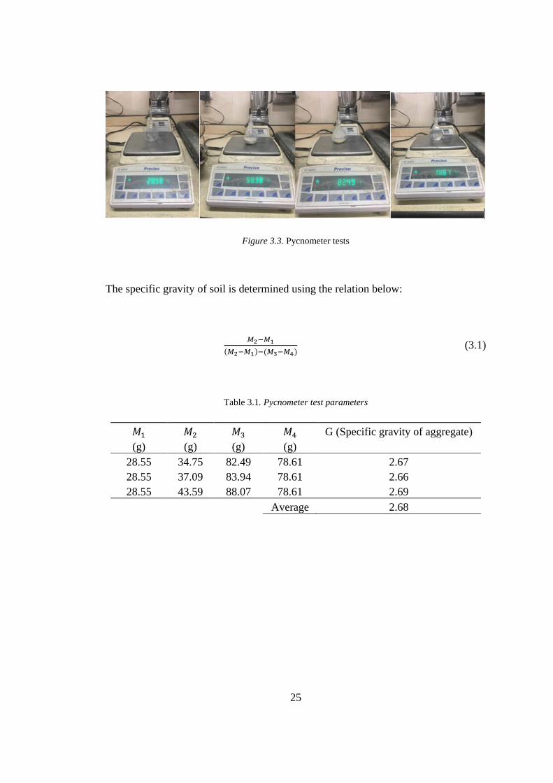
Figure 3.3. Pycnometer tests ...................................................................................... 25
Figure 3.4. Additives .................................................................................................. 26
Figure 3.5. Drawing of FBD mold in SolidWorks ..................................................... 27
Figure 3.6. Used molds with varying diameters 100 mm to 200 mm ........................ 28
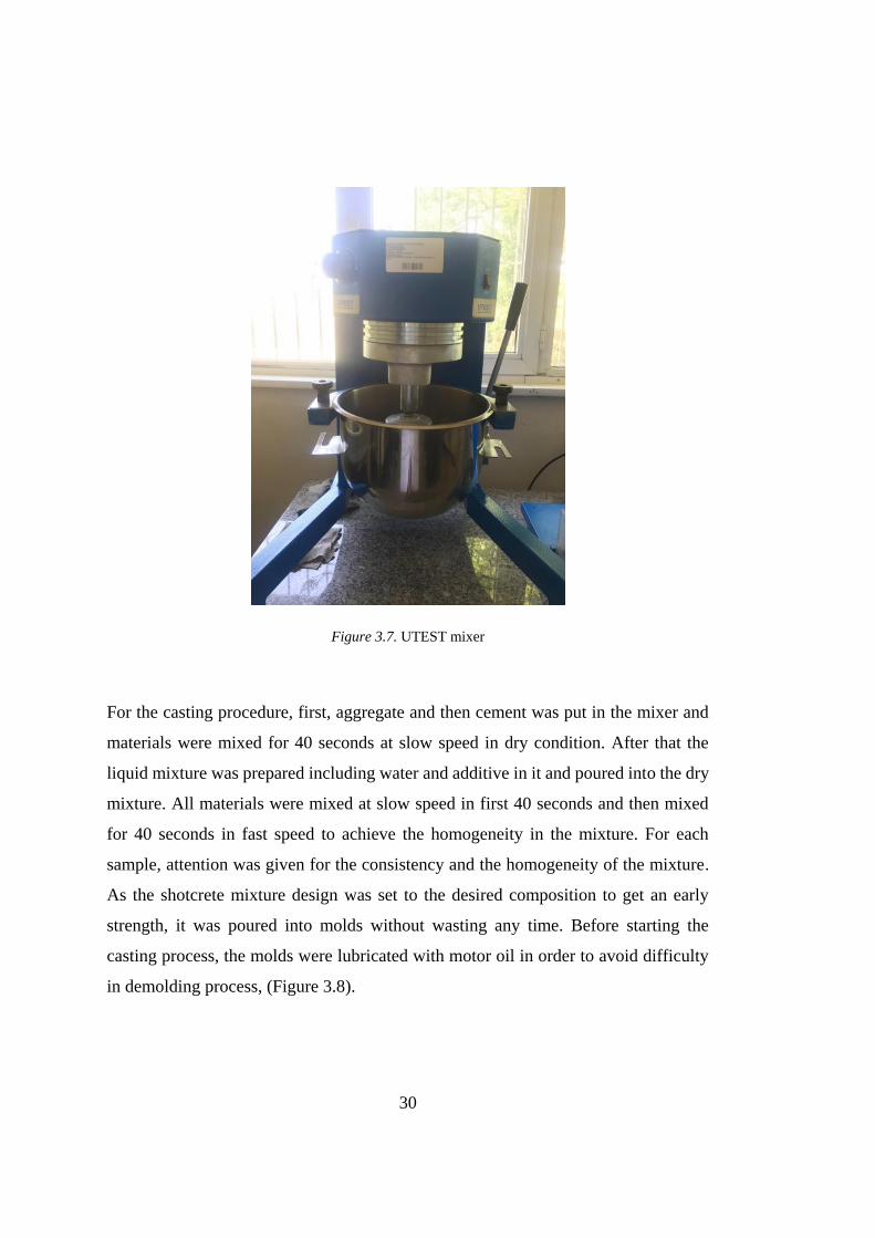
Figure 3.7. UTEST mixer........................................................................................... 30
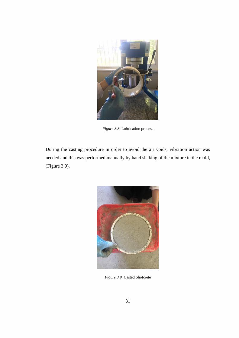
Figure 3.8. Lubrication process .................................................................................. 31
Figure 3.9. Casted Shotcrete ...................................................................................... 31
Figure 3.10. Successful and unsuccessful casting products ....................................... 32
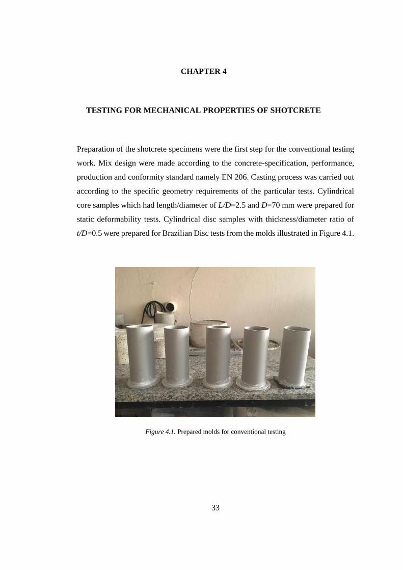
Figure 4.1. Prepared molds for conventional testing ................................................. 33
Figure 4.2. Cylindrical samples taken out of molds for static deformability test ...... 34
Figure 4.3. Static Deformability Test Setup............................................................... 35
Figure 4.4. Lateral strain vs axial strain graph ........................................................... 37

xviii
Figure 4.5. Stress vs lateral strain and axial strain graph .......................................... 37
Figure 4.6. Development of Young’s modulus with early age of shotcrete compiled
from various research by (Chang, 1994) ................................................................... 38
Figure 4.7. UCS results of various researchers compiled by Chang (1994) .............. 39
Figure 4.8. Variation of Poisson’s ratio with time (Aydan et al., 1992) ................... 40
Figure 4.9. Brazilian Disc Test set up ........................................................................ 42
Figure 4.10. A typical Brazilian Disc sample with central crack clearly visible ....... 43
Figure 4.11. Force-Displacement curve of a Brazilian Disc test specimen ............... 44
Figure 4.12. Specimen subjected to a uniform diametric loading (Wang et al.,2004)
................................................................................................................................... 47
Figure 4.13. Tensile strength versus specimen diameter using Wang approach ....... 49
Figure 4.14. The ratio of the tensile strengths from FBD and BD with varying diameter
................................................................................................................................... 50
Figure 4.15. Tensile strength versus specimen diameter using Keles and Tutluoglu
approach ..................................................................................................................... 52
Figure 4.16. The ratio of tensile strengths from FBD and BD with related diameters
................................................................................................................................... 53
Figure 4.17. Bazant’s size effect investigation (Bazant et al., 1991) ........................ 54
Figure 5.1. A typical Force-Displacement curve of a Flattened Brazilian Disc test . 57
Figure 5.2. A typical experimental critical crack length measurement ..................... 58
Figure 5.3. Name code of tested FBD specimens ...................................................... 62
Figure 5.4. FBD specimen geometry ......................................................................... 63
Figure 5.5. Name code of tested FBD specimens ...................................................... 66
Figure 6.1. KIC values of FBD tested specimens having various diameters .............. 73
Figure 6.2. Dimensionless critical crack length of FBD tested specimens ............... 74
Figure 6.3. Average KIC values changing with the curing time of shotcrete ............. 78
Figure 6.4. The relation between σt W and KIC ........................................................... 79
Figure 6.5. The relation between σt,K T and KIC ......................................................... 80
Figure 6.6. Dimensionless toughness over tensile strength ratio ............................... 81
Figure 0.1. Static deformability test graph of S_SD_1 .............................................. 95
xix
Figure 0.2. Static deformability test graph of S_SD_1 .............................................. 95
Figure 0.3. Static deformability test graph of S_SD_2 .............................................. 96
Figure 0.4. Static deformability test graph of S_SD_2 .............................................. 96
Figure 0.5. Static deformability test graph of S_SD_3 .............................................. 97
Figure 0.6. Static deformability test graph of S_SD_3 .............................................. 97
Figure 0.7. Static deformability test graph of S_SD_4 .............................................. 98
Figure 0.8. Static deformability test graph of S_SD_4 .............................................. 98
Figure 0.9. Static deformability test graph of S_SD_5 .............................................. 99
Figure 0.10. Static deformability test graph of S_SD_5 ............................................ 99
Figure 0.11. Brazilian Disc test graph of S_BD_1 .................................................. 100
Figure 0.12. Brazilian Disc test graph of S_BD_2 .................................................. 100
Figure 0.13. Brazilian Disc test graph of S_BD_3 .................................................. 101
Figure 0.14. Brazilian Disc test graph of S_BD_4 .................................................. 101
Figure 0.15. Brazilian Disc test graph of S_BD_5 .................................................. 102
Figure 0.16. Flattened Brazilian Disc test graph of S100_s1 ................................... 103
Figure 0.17. Flattened Brazilian Disc test graph of S100_s2 ................................... 103
Figure 0.18. Flattened Brazilian Disc test graph of S100_s3 ................................... 104
Figure 0.19. Flattened Brazilian Disc test graph of S100_s4 ................................... 104
Figure 0.20. Flattened Brazilian Disc test graph of S100_s5 ................................... 105
Figure 0.21. Flattened Brazilian Disc test graph of S120_s1 ................................... 105
Figure 0.22. Flattened Brazilian Disc test graph of S120_s2 ................................... 106
Figure 0.23. Flattened Brazilian Disc test graph of S120_s3 ................................... 106
Figure 0.24. Flattened Brazilian Disc test graph of S120_s4 ................................... 107
Figure 0.25. Flattened Brazilian Disc test graph of S120_s5 ................................... 107
Figure 0.26. Flattened Brazilian Disc test graph of S120_s6 ................................... 108
Figure 0.27. Flattened Brazilian Disc test graph of S140_s1 ................................... 108
Figure 0.28. Flattened Brazilian Disc test graph of S140_s2 ................................... 109
Figure 0.29. Flattened Brazilian Disc test graph of S140_s3 ................................... 109
Figure 0.30. Flattened Brazilian Disc test graph of S140_s4 ................................... 110
Figure 0.31. Flattened Brazilian Disc test graph of S140_s5 ................................... 110

xx
Figure 0.32. Flattened Brazilian Disc test graph of S160_s1 .................................. 111
Figure 0.33. Flattened Brazilian Disc test graph of S160_s2 .................................. 111
Figure 0.34. Flattened Brazilian Disc test graph of S160_s3 .................................. 112
Figure 0.35. Flattened Brazilian Disc test graph of S160_s4 .................................. 112
Figure 0.36. Flattened Brazilian Disc test graph of S160_s5 .................................. 113
Figure 0.37. Flattened Brazilian Disc test graph of S180_s1 .................................. 113
Figure 0.38. Flattened Brazilian Disc test graph of S180_s2 .................................. 114
Figure 0.39. Flattened Brazilian Disc test graph of S180_s3 .................................. 114
Figure 0.40. Flattened Brazilian Disc test graph of S180_s4 .................................. 115
Figure 0.41. Flattened Brazilian Disc test graph of S180_s5 .................................. 115
Figure 0.42. Flattened Brazilian Disc test graph of S200_s1 .................................. 116
Figure 0.43. Flattened Brazilian Disc test graph of S200_s2 .................................. 116
Figure 0.44. Flattened Brazilian Disc test graph of S200_s3 .................................. 117
Figure 0.45. Flattened Brazilian Disc test graph of S200_s4 .................................. 117
Figure 0.46. Flattened Brazilian Disc test graph of S160-1D-s1 ............................. 118
Figure 0.47. Flattened Brazilian Disc test graph of S160-1D-s2 ............................. 118
Figure 0.48. Flattened Brazilian Disc test graph of S160-1D-s3 ............................. 119
Figure 0.49. Flattened Brazilian Disc test graph of S160-1D-s4 ............................. 119
Figure 0.50. Flattened Brazilian Disc test graph of S160-2D-s1 ............................. 120
Figure 0.51. Flattened Brazilian Disc test graph of S160-2D-s2 ............................. 120
Figure 0.52. Flattened Brazilian Disc test graph of S160-2D-s3 ............................. 121
Figure 0.53. Flattened Brazilian Disc test graph of S160-2D-s4 ............................. 121
Figure 0.54. Flattened Brazilian Disc test graph of S160-3D-s1 ............................. 122
Figure 0.55. Flattened Brazilian Disc test graph of S160-3D-s2 ............................. 122
Figure 0.56. Flattened Brazilian Disc test graph of S160-3D-s3 ............................. 123
Figure 0.57. Flattened Brazilian Disc test graph of S160-5D-s1 ............................. 123
Figure 0.58. Flattened Brazilian Disc test graph of S160-5D-s2 ............................. 124
Figure 0.59. Flattened Brazilian Disc test graph of S160-5D-s3 ............................. 124
Figure 0.60. Flattened Brazilian Disc test graph of S160-5D-s4 ............................. 125
Figure 0.61. FBD test crack measurement of the sample S100_s1 ......................... 127

xxi
Figure 0.62. FBD test crack measurement of the sample S100_s2 .......................... 127
Figure 0.63. FBD test crack measurement of the sample S100_s3 .......................... 128
Figure 0.64. FBD test crack measurement of the sample S100_s4 .......................... 128
Figure 0.65. FBD test crack measurement of the sample S100_s5 .......................... 129
Figure 0.66. FBD test crack measurement of the sample S120_s1 .......................... 129
Figure 0.67. FBD test crack measurement of the sample S120_s2 .......................... 130
Figure 0.68. FBD test crack measurement of the sample S120_s3 .......................... 130
Figure 0.69. FBD test crack measurement of the sample S120_s4 .......................... 131
Figure 0.70. FBD test crack measurement of the sample S120_s5 .......................... 131
Figure 0.71. FBD test crack measurement of the sample S120_s6 .......................... 132
Figure 0.72. FBD test crack measurement of the sample S140_s1 .......................... 132
Figure 0.73. FBD test crack measurement of the sample S140_s2 .......................... 133
Figure 0.74. FBD test crack measurement of the sample S140_s3 .......................... 133
Figure 0.75. FBD test crack measurement of the sample S140_s4 .......................... 134
Figure 0.76. FBD test crack measurement of the sample S140_s5 .......................... 134
Figure 0.77. FBD test crack measurement of the sample S160_s1 .......................... 135
Figure 0.78. FBD test crack measurement of the sample S160_s2 .......................... 135
Figure 0.79. FBD test crack measurement of the sample S160_s3 .......................... 136
Figure 0.80. FBD test crack measurement of the sample S160_s4 .......................... 136
Figure 0.81. FBD test crack measurement of the sample S160_s5 .......................... 137
Figure 0.82. FBD test crack measurement of the sample S180_s1 .......................... 137
Figure 0.83. FBD test crack measurement of the sample S180_s2 .......................... 138
Figure 0.84. FBD test crack measurement of the sample S180_s3 .......................... 138
Figure 0.85. FBD test crack measurement of the sample S180_s4 .......................... 139
Figure 0.86. FBD test crack measurement of the sample S180_s5 .......................... 139
Figure 0.87. FBD test crack measurement of the sample S200_s1 .......................... 140
Figure 0.88. FBD test crack measurement of the sample S200_s2 .......................... 140
Figure 0.89. FBD test crack measurement of the sample S200_s3 .......................... 141
Figure 0.90. FBD test crack measurement of the sample S200_s4 .......................... 141

xxii
LIST OF ABBREVIATIONS
ABBREVIATIONS
2D: two-dimensional
3D: three-dimensional
BDT : Brazilian disc test
CB : Chevron bend
CCNBD : Cracked chevron notched Brazilian disc
CPD: Crack propagation direction
CPE8: Continuum plane strain eight noded element
CSTBD : Cracked straight through Brazilian disc
FBD : Flattened Brazilian disc
ISRM : International Society for Rock Mechanics
LEFM: Linear elastic fracture mechanics
LVDT: Linear variable differential transformer
MTS: Maximum tangential stress
SCB : Semi-circular bending
SIF: Stress intensity factor
SNDB : Straight-notched disc bending
SR: Short-rod
UCS : Uniaxial Compressive Strength
xxiii
LIST OF SYMBOLS
SYMBOLS
a: half of crack length
A: mesh size
A: andesite
D: specimen diameter
de: distance of crack tip to central load application point
E: Elastic Modulus
G : energy release rate
Gc : critical energy release rate
J: J integral
K: stress intensity factor
KC: critical stress intensity factor
𝐾I : mode I stress intensity factor (opening mode)
𝐾II : mode II stress intensity factor (shearing mode)
𝐾III : mode III stress intensity factor (tearing mode)
KIc : mode I fracture toughness
KIIc : mode II fracture toughness
L: half of flattened length
P: applied concentrated load
Pmax: failure load

xxiv
Pmin: local minimum load
R: disc radius
rc: radius of contour integral region
S11 : normal stress in x-direction
S22 : normal stress in y-direction
S33 : normal stress in z-direction
S12 : shear stress in xy-direction
S: span length
t: specimen thickness
Y : dimensionless stress intensity factor
YI : mode I dimensionless stress intensity factor
YII : mode II dimensionless stress intensity factor
Yımax : maximum dimensionless stress intensity factor
w : projected width over loaded section
: half of loading angle
ε : Strain
σ : stress
𝜎1 : maximum principal stress
𝜎3 : minimum principal stress
𝜎𝑡 : tensile strength
α : a/R

xxv
τ : shear stress
µ: shear modulus
𝜗 : Poisson’s Ratio
θ : crack propagation angle
tc: curing time in days
𝜎𝑡: tensile strength


1
CHAPTER 1
1. INTRODUCTION
1.1. General
According to the data from the National Institute for Science and Technology and the
Bettelle Memorial Institute, in one year 119 billion dollars were spent because of
fracture related failures in 1983. The money has an incontrovertible significance;
however, the price of many failures in human life and also physical injuries are more
important than the dollars, (Anderson, 2005).
Defects in the materials, lack of information about the loading or environment,
improper design and defects in structures can cause catastrophic failures.
In the respect of both structural and mining engineering, Rossmanith said that the main
questions are respectively: “how the failure load of these flawed structures can be
estimated? Which kind of combinations of load and parameters of flaw geometry
causes the failure? Moreover, which material variables are the fracture process
conducted by?” (Rossmanith, 1983).
In 1950’s and 1960’s, Fracture Engineering eventually arise to find out the causes of
cracks in various engineering materials. There are several engineering materials such
as metal, rock, concrete and ceramics. Rock fracture mechanics is the science that
identifies how the crack starts and disseminates under the applied loads in rock
engineering. The crack resistance at the beginning of the crack growth is specified by
fracture toughness parameter and this is a very active area of the current research.
The stability of underground engineering structures may be possible by supporting the
cavities opened in the structures rapidly with lower cost. Shotcrete technology has
improved recently with the findings and innovations in installation equipment and

2
material technology. Although, shotcrete applications go back a long way around the
beginning of 20th century, structural integrity of shotcrete is a relatively a new field
of research area which needs to be investigated in detail. Nowadays, underground
mine openings, tunnels, and the galleries of many purposes are being stabilized by
shotcrete support systems. As most of the time shotcrete is applied just after its
preparation on site, it is difficult to conduct a detailed laboratory analysis. Detailed
laboratory testing can be done if a proper mixture of shotcrete can be prepared; so that
shotcrete in the field practice is simulated closely.
1.2. Statement of the Problem
Although, shotcrete is a widely used heterogeneous material that particularly used as
a support system, the crack behavior of it has not been focused enough even though
one of the most important weakness of it is cracks. Most of the studies on shotcrete is
based on laboratory tests to determine its mechanical properties, strength, setting time
or rebound rate. So far, not enough attention is paid to the fracture mechanics and
crack propagation characteristics of shotcrete, which is one of the most important
consideration for the field of engineering.
Mode I fracture toughness is a measure of the fracture energy to propagate a crack
under tension in materials. This parameter is important also in the preventing efforts
of propagation of a pre-existing defect. Fracture toughness tests are commonly carried
out with beam and disc or cylinder-type specimen geometries. One current trend in
fracture toughness testing is to minimize the specimen geometry effect on pure tensile
mode crack opening. Specimen geometry is associated with a size effect issue.
Size effect on facture toughness of rocks has been frequently investigated. However,
rock fracture toughness testing is usually restricted to the core sample diameters which
may go up to around 100 mm in practice. It has not been possible to work with large
range of diameters. Sizes of specimens were limited, in particular in circular
geometries such as FBD geometry, depending on the diameter of the core drilling
3
machine. Research on internal characteristics and mechanical properties of shotcrete
is still in progress in literature. It is worth to carry out an investigation about the size
effect on fracture toughness of cementitious material.
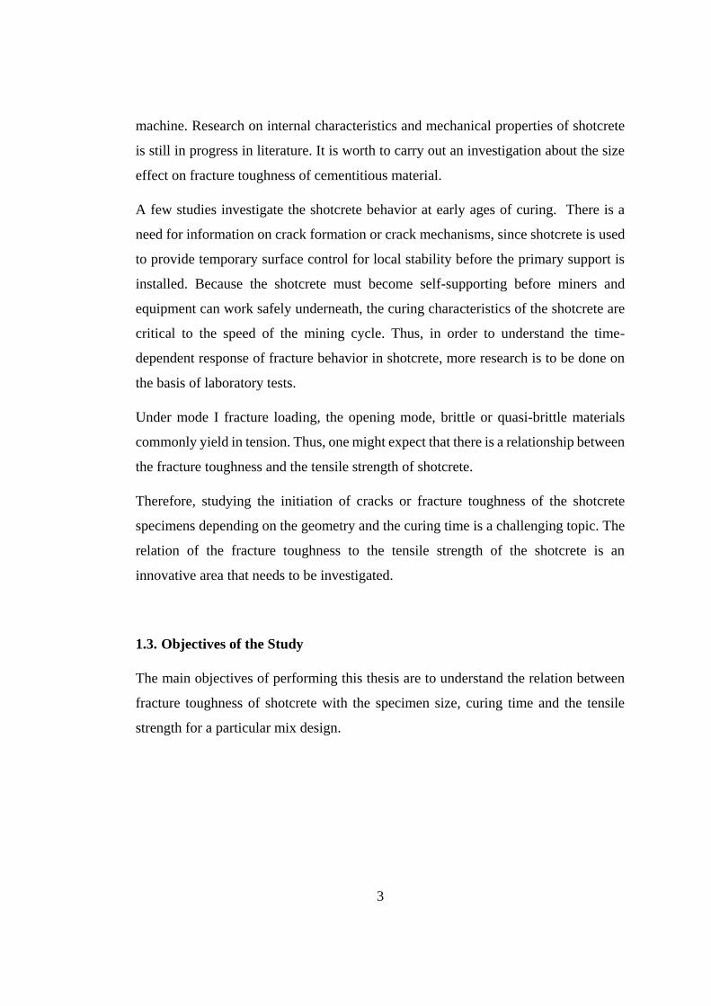
A few studies investigate the shotcrete behavior at early ages of curing. There is a
need for information on crack formation or crack mechanisms, since shotcrete is used
to provide temporary surface control for local stability before the primary support is
installed. Because the shotcrete must become self-supporting before miners and
equipment can work safely underneath, the curing characteristics of the shotcrete are
critical to the speed of the mining cycle. Thus, in order to understand the time-
dependent response of fracture behavior in shotcrete, more research is to be done on
the basis of laboratory tests.
Under mode I fracture loading, the opening mode, brittle or quasi-brittle materials
commonly yield in tension. Thus, one might expect that there is a relationship between
the fracture toughness and the tensile strength of shotcrete.
Therefore, studying the initiation of cracks or fracture toughness of the shotcrete
specimens depending on the geometry and the curing time is a challenging topic. The
relation of the fracture toughness to the tensile strength of the shotcrete is an
innovative area that needs to be investigated.
1.3. Objectives of the Study
The main objectives of performing this thesis are to understand the relation between
fracture toughness of shotcrete with the specimen size, curing time and the tensile
strength for a particular mix design.

4
1.4. Methodology of the Study
Cementitious materials like shotcrete-concrete generally exhibit high compressive
strength, low tensile strength. So the mode I, in other words tensile opening mode is a
crucial loading mode for not only shotcrete but also for brittle materials such as rocks.
ISRM and ASTM suggested many methods to measure the rock fracture toughness.
The main proposed methods by International Society for Rock Mechanics (ISRM),
are:
Short rod (SR) (Ouchterlony, 1988),
Chevron bend (CB) (Ouchterlony, 1988),
Cracked chevron notched Brazilian disc (CCNBD) (Fowell, 1995)
Semi-circular bending (Kuruppu et al., 2015)
Brazilian type methods which were preferable since relatively simple both in specimen
preparation and also compressive loading on disc specimens while testing include;
Cracked chevron notched Brazilian disc (CCNBD), (Sheity, D. K.,
Rosenfield, A. R., & Duckworth, W. H. (1985)
Cracked straight through Brazilian disc (CSTBD)
Semi-circular bending test (SCB) (Chong and Kuruppu, 1984)
Brazilian disc (BD) (Guo et al., 1993)
Flattened Brazilian disc (FBD) (Wang and Xing, 1999)
The reason for selection of the Flattened Brazilian Disc method is the easiness of
sample preparation and testing procedure. Compressive loading in fracture testing and
indirectly generating tensile splitting are attractive for brittle materials. Although, it is
necessary to prepare a very precise samples for FBD testing, the usage of 3D printing
technology for shotcrete casting process provided the desired geometric accuracy.
Moreover, 3D printing technology made preparation of specimens in different sizes
5
possible. A wide range of specimen with varying diameters were tested to measure
tensile strength and mode I fracture toughness of shotcrete.
The experimental work started with the preparation of the shotcrete specimens. In the
preparation of shotcrete samples, attention was paid to use the same ingredients for
each sample and to prepare with the same equipment under the same laboratory
conditions in order to interpret the test results correctly. Five samples were molded
and tested for each group of varying specimen sizes in order to increase statistical
quality of the test results.
For all tests, MTS 815 Rock Testing Machine in laboratory was used. Five specimens
were prepared for each diameter and curing time group.
First, conventional mechanical property testing work was conducted. Static
deformability test and uniaxial compressive strength tests were conducted in order
both to check the mechanical properties of the shotcrete and to validate the mixture
according to its mechanical properties in the literature. The conventional Brazilian
disc test was conducted next to measure the tensile strength with regular testing
method.
Finally, as the main part, mode I fracture toughness tests with Flattened Brazilian Disc
geometry were carried out to split the samples into two. One investigation was the size
effect on fracture toughness with constant curing time and changing diameters and the
second one was performed to analyse the effect of curing time on fracture toughness
with constant diameter and various curing time. Moreover, in order to determine the
relation between fracture toughness and the tensile strength, conventional Brazilian
test results were compared to the results of Flattened Brazilian Disk tests. For the
evaluation of experimental results, equations from a similar work were adopted.

6
1.5. Organization of Thesis
This thesis is divided into six chapter. Following this introduction. Chapter 2 presents
a general review of the literature about the basics of fracture mechanic and its
significance for the main research problem. In Chapter 2, description of the different
fracture toughness testing methods is provided. Experimental method used to
determine mode I fracture toughness and its background are explained as well as
fracture mechanics of shotcrete. Chapter 3 presents a description of the properties of
shotcrete mixture and its ingredients. It continues with the shotcrete mix design and
laboratory work related to the casting process. Chapter 4 presents a detailed
description of the laboratory work and the results of all conventional experimental
study, including static deformability tests, Brazilian disc test, and the most importantly
Flattened Brazilian Disc tests to investigate fracture toughness and to the factors
affecting its value. Chapter 5 presents evaluation of the results, discussion of the all
experiments carried out, and the interpretation of these results with the help of
previous studies in literature. Finally, Chapter 6 presents conclusion and the findings
of this study as well as recommendations for further research in this field.

7
CHAPTER 2
2. THEORETICAL BACKGROUND OF FRACTURE MECHANICS
2.1. History of Fracture Mechanics
In the early Renaissance, the concept of fracture had been scientifically evaluated as
scaling of fracture and experiments were conducted on iron wires by Leonardo da
Vinci for the first time (1452-1519), (Figure 2.1), (Gross,2014).
Figure 2.1. Leonardo da Vinci fracture test setup (Gross, 2014)
Afterwards, Galileo Galilei (1564–1642) who was known as the founder of modern
mechanics by his contributions from his well-known “Dialog”, made correct
inferences that the fracture forces of column under tension were related to the cross
sectional area, and also he stated that the bending moment was the crucial loading type
for the fracture of beams, (Figure 2.2), (Cotterel, 2002).

8
Figure 2.2. Galileo Galilei tensile test setup (Gross, 2014)
The most punctual work was done by Griffith (1921). He carried out an analysis for
actual cracks. Even though, Griffith’s theory was so important, it was limited for some
highly brittle materials such as glass. In the early 1960s, with the development of the
discipline that we called “fracture mechanics”, Irwin (1958) who was a professor from
Lehigh University, examined plasticity in detail. He extended the Griffth’s theory.
Irwin proposed that the stress intensity factor concept could be used for the calculation
of stress field around the crack tip.
Applications of engineering fracture mechanics to brittle materials developed with an
important delay in comparison to ductile materials. Considering the underground
mines, tunnels in galleries etc., rock fracture problem has a significant role in
collapses. At the early sixties, Griffith’s model found the roles in applications
involving stone and concrete type materials. The friction between crack faces was
established byMc Clintock and Walsh (1962). They modified Griffith’s theory and
investigated the crack closure in compression, whereas Kaplan (1961) have published
the first experimental study about the possibility of applying linear elastic fracture
mechanics to concrete. In 1965 Bieniawski and Hoek was performed the early research
about rocks, in South Africa, where mine disappointments were earnest issues to be
comprehended (Ceriolo and Tommaso, 1998).

9
2.2. Basics of Fracture Mechanics
2.2.1. Fracture Modes
There are three main ways named as mode I, mode II and mode III for cracks to initiate
and propagate in a material, (Figure 2.3).
Figure 2.3. Fracture modes (Key to Metals Database, 2010)
Mode I: In mode I, also known as tensile opening mode, direction normal to the crack
plane separates the faces of the cracks.
Mode II: In mode II, also named as in-plane sliding or shear mode, both crack faces
are in the direction of crack front normal.
Mode III: In mode III, also named as the tearing or out of plane mode, the crack faces
are sheared parallel to the crack front.
Crack formations can occur by any of these three modes. Moreover, combinations of
these modes are also possible such as mode I and mode II can occur simultaneously.
In such a case it is called as mixed mode. Mode I is the essential failure mode for
brittle material since brittle materials are weak under tension.

10
2.2.2. Stress Intensity Factor
Stress intensity factor, K is used for predicting the stress state around the tip of the
crack. K depends on the size and location of the crack as well as sample geometry. It
is important that the maximum stress around the tip of the crack not to exceed the
fracture toughness. Otherwise, if K exceeds the fracture toughness values, crack
initiates and propagates.
Formula for calculating the stress intensity factor for beam and plate type geometries
is given below:
𝐾 = 𝜎√𝑎 × 𝜋 × 𝑓(𝑎
𝑤) (2.1)
where:
σ: remote stress applied to component (MPa)
a: crack length (m)
f (a/w): correction factor that depends on specimen and crack geometry
w: specimen width or beam depth (m)
2.2.3. Fracture Toughness
Fracture toughness, KC is the critical value of stress intensity factor that represents the
material’s resistance to fracture. It depending on loading rate, temperature,
environment, composition and microstructure with geometric effects.
The mode I, opening mode, fracture toughness of concrete can be expressed by the
critical stress intensity factor, 𝐾𝐼𝐶. Similarly, especially in concrete related studies, 𝐺𝐶,
energy release rate usually used to express the fracture toughness. The term 𝐺𝑐, called
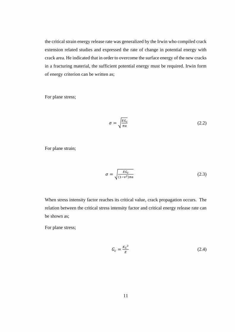
11
the critical strain energy release rate was generalized by the Irwin who compiled crack
extension related studies and expressed the rate of change in potential energy with
crack area. He indicated that in order to overcome the surface energy of the new cracks
in a fracturing material, the sufficient potential energy must be required. Irwin form
of energy criterion can be written as;
For plane stress;
𝜎 = √𝐸𝐺𝑐
𝜋𝑎 (2.2)
For plane strain;
𝜎 = √𝐸𝐺𝑐
(1−𝜈2)𝜋𝑎 (2.3)
When stress intensity factor reaches its critical value, crack propagation occurs. The
relation between the critical stress intensity factor and critical energy release rate can
be shown as;
For plane stress;
𝐺𝑐 =𝐾𝐶
2
𝐸 (2.4)

12
For plane strain;
𝐺𝐶 = 𝐾𝐶2 (
1−𝜈2
𝐸) (2.5)
GC: Critical energy release rate (MPa.m)
E: Elastic Modulus (MPa)
υ: Poisson’s ratio
KC: Critical stress intensity factor (MPa√m)
2.2.4. Linear Elastic Fracture Mechanics
Linear Elastic Fracture Mechanics works under the assumption of the material being
linear elastic and isotropic. Assuming that the material is linear elastic and isotropic
indicate that the material properties are independent of direction. At the same time,
elastic modulus, E and Poisson’s ratio, υ are two independent elastic constant that
material has. In LEFM assumption, considering the theory of elasticity, the stress field
around the crack tip can be calculated. However, Linear Elastic Fracture Mechanics,
LEFM, is only applicable when the inelastic deformation around the crack path is
relatively smaller compare to the size of a crack.
Irwin found a method for calculating the amount of energy available for fracture.
𝜎𝑖𝑗 = (𝐾𝐼
√2𝜋𝑟)𝑓𝑖𝑗(𝜃) (2.6)
𝜎𝑖𝑗 : Cauchy Stress
𝐾𝐼 : stress intensity factor
r: the distance from the crack tip
13
𝜃 : angle with respect to the plane of the crack
𝑓𝑖𝑗 : function depending on the crack geometry and loading conditions
In general, LEFM is valid when the nonlinear material deformation at the crack tip is
small enough. In order to characterize nonlinear behavior like plastic deformation for
many materials, there was a need for an alternative fracture mechanics model namely
Elastic-Plastic Fracture Mechanics. Unlike LEFM, the material is assumed to be
isotropic and elasto-plastic.
2.3. Fracture Toughness Testing with Flattened Brazilian Disc Test Method
Brazilian tensile strength testing specimen geometry was suggested by Guo et al.
(1993) as a mode I fracture toughness test method so that without machining a notch
or crack, mode I fracture toughness (Kıc) may be determined.
The relation between stress intensity factors (SIF) were studied by Guo et al. (1993).
A formula using dimensionless stress intensity factor, YI and dimensionless crack
length, a/R was derived by numerical integration method. From the numerical
solution, it was found out that dimensionless stress intensity factor could be expressed
as a function of dimensionless crack length.
Changing the loading angles between 5°- 50°, Guo et al., 1993 showed the relationship
between different crack lengths and the stress intensity factors for Flattened Brazilian
Disk type geometry.
After numerical interpretations, formula for BDT under mode I fracture toughness was
derived as follows (Guo et al., 1993):
𝐾𝐼𝐶 = 𝐵 × 𝑃𝑚𝑖𝑛 × 𝑌𝐼(𝑎
𝑅) (2.7)

14
Where:
𝐾𝐼𝐶: mode I fracture toughness
B: the constant dependent on geometry of the specimen
B: 2
√𝑅×𝑡×𝑎×𝜋√𝜋 (2.8)
𝑃𝑚𝑖𝑛: local minimum load
R: disc radius
t: disc thickness
𝑌𝐼(𝑎
𝑅): dimensionless stress intensity factor
a: half of crack length
a/R: dimensionless crack length
Method suggested by Guo et. Al (1993) has some limitations and problematic cases
such as: crack initiation at the center and crack propagation along vertical axis is not
guaranteed, also it could not explain the relation between loading angle and where the
crack initiates (Wang and Xing, 1999). In the problems that crack initiated at the center
inconsistent SIF values resulted due to the assumption of uniform arc loading and
wrong selection of domain, (Figure 2.4).
15
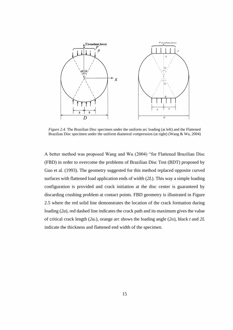
Figure 2.4. The Brazilian Disc specimen under the uniform arc loading (at left) and the Flattened
Brazilian Disc specimen under the uniform diametral compression (at right) (Wang & Wu, 2004)
A better method was proposed Wang and Wu (2004) “for Flattened Brazilian Disc
(FBD) in order to overcome the problems of Brazilian Disc Test (BDT) proposed by
Guo et al. (1993). The geometry suggested for this method replaced opposite curved
surfaces with flattened load application ends of width (2L). This way a simple loading
configuration is provided and crack initiation at the disc center is guaranteed by
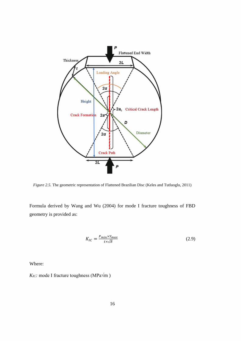
discarding crushing problem at contact points. FBD geometry is illustrated in Figure
2.5 where the red solid line demonstrates the location of the crack formation during
loading (2a), red dashed line indicates the crack path and its maximum gives the value
of critical crack length (2ac), orange arc shows the loading angle (2α), black t and 2L
indicate the thickness and flattened end width of the specimen.
16
Figure 2.5. The geometric representation of Flattened Brazilian Disc (Keles and Tutluoglu, 2011)
Formula derived by Wang and Wu (2004) for mode I fracture toughness of FBD
geometry is provided as:
𝐾𝐼𝐶 =𝑃𝑚𝑖𝑛×𝑌𝑚𝑎𝑥
𝑡×√𝑅 (2.9)
Where:
KIC: mode I fracture toughness (MPa√m )
17
Pmin: local minimum load (MN)
𝑌Imax: maximum dimensionless stress intensity factor
R: disc radius (m)
t: disc thickness (m)
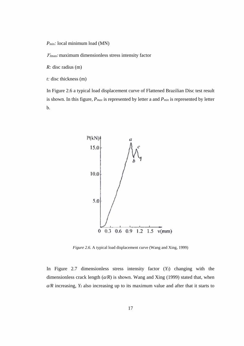
In Figure 2.6 a typical load displacement curve of Flattened Brazilian Disc test result
is shown. In this figure, Pmax is represented by letter a and Pmin is represented by letter
b.
Figure 2.6. A typical load displacement curve (Wang and Xing, 1999)
In Figure 2.7 dimensionless stress intensity factor (YI) changing with the
dimensionless crack length (a/R) is shown. Wang and Xing (1999) stated that, when
a/R increasing, YI also increasing up to its maximum value and after that it starts to

18
decrease. When YI reaches its maximum, it is called maximum dimensionless stress
intensity factor at dimensionless critical crack length. In this circumstances,
dimensionless stress intensity factor only depends on the loading angle and it can be
calculated numerically.
Figure 2.7. Maximum dimensionless stress intensity factor represented by Wang and Xing (Wang and
Xing, 1999)
2.4. Fracture Mechanics of Concrete
Beginning of fracture mechanics of concrete was by Kaplan (Kaplan, 1961) who
conducted experiments with four point bending of notched beams at various sizes. His
experiments showed that fracture toughness of concrete beams were changing
depending on their geometry and size. After that Kesler, Naus and Lott (1971) stated
that the LEFM that Kaplan used was inapplicable on concrete structures with sharp
cracks. Walsh’s experimental works supported Kaplan’s findings. (Walsh, 1979). In
the wake of experimental results on notched concrete beams and their relation with
the KC, in order to describe the crack growth on concrete at least two fracture
parameters were needed. In order to understand and model the behavior of concrete,
a major improvement as made in 1976 by Hillerborg, Modeer and Petersson was

19
fictitious crack model. In 1976, Crack band model was proposed by Bazant in order
to explain the fracture process zone on concrete with using the concept of the strain-
softening, (Bazant, 1976). Jenq and Shah (1985) proposed the two-parameter model
which assumed a crack tip singularity in front of the real crack. (Carpinteri, 1984)
described fracture behavior of the concrete by expressing the rate of change of strain
energy density with the crack growth. Two-parameter model was used by Karihaloo
and Nallathambi to propose effective crack model which assumes a sharp crack in
front of the real crack (Karihaloo and Nallathambi, 1989).
Almost all the work summarized is related to the size effect issues in concrete beams.
Concrete and shotcrete are structurally very similar materials; the difference lies in the
application. Testing work here originally involves splitting disc type specimen
geometries for which tensile cracking along the central line is generated by a
compressive at the ends.

21
CHAPTER 3
3. SHOTCRETE MIXTURE SETUP
In early 1900’s the spraying a cement-sand mixture was developed with the trade name
of Gunite and ever since it has been used in the mining industry. However, it took fifty
years to use the same process with a coarse aggregate, now called shotcrete. After that,
shotcrete was used for the first time on a tunnel project in Austria in mid-50’s. it did
not attract much attention for ten years until Burnaby-Vancouver railway tunnel on
the North American continent was under construction. After it was introduced, it
attracted attention in 1967 and several Canadian and American mining firms had
experimented or started to use shotcrete. (Miner, 1973)
The reason why shotcrete is widely used especially in underground works and tunnel
construction as a rock support is due to the continuously developed mining industry
and their constant search for ways and methods to reduce costs at the same time. Thus,
investigation of the fracture properties of all composites (concrete, shotcrete, etc.) that
are used in the underground openings is crucial in order to reach safe working
environment and conduct safe operations in mining and civil engineering industry.
3.1. Shotcrete Mixture Ingredients
The ingredients of shotcrete mixture are Portland cement, aggregate, water and
additives when necessary. In order to get the optimum strength and proper spraying
ability of shotcrete mixture, correct proportions of ingredients and correct
water/cement ratio are essential.
It is known that the water/cement ratio of the shotcrete should be between 0.35-0.50
(M.G. Alexander and R. Heiyantuduwa, 2009). The required 7 days strength of
22
shotcrete is between 25-30 MPa and 28 days strength is 35-40 MPa. In this study
water/cement ratio selected as 0.5. According to the suggested concrete mixture
properties standard TS EN 2016-1, concrete with 0.5 water cement ratio refer to C30
which is the minimum concrete grade for durable and long-lasting structures.
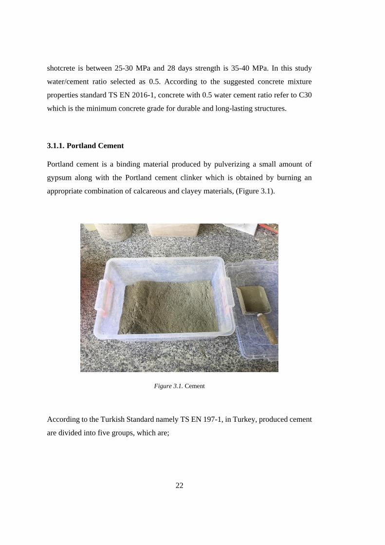
3.1.1. Portland Cement
Portland cement is a binding material produced by pulverizing a small amount of
gypsum along with the Portland cement clinker which is obtained by burning an
appropriate combination of calcareous and clayey materials, (Figure 3.1).
Figure 3.1. Cement
According to the Turkish Standard namely TS EN 197-1, in Turkey, produced cement
are divided into five groups, which are;
23
CEM I; Portland Cement
CEM II; Portland-Composed Cement
CEM III; Blast Furnace Slag Cement
CEM IV; Pozzolanic Cement
CEM V; Composed Cement (Erdoğan, 2013)
The amount of cement usage is directly effective in determining the mechanical
properties, especially strength, of the shotcrete. According to the application area the
amount of cement should be selected. In experimental studies, CEM I 42.5 R was used
in the shotcrete mixture. 42.5 means the 28-day strength of shotcrete should be 42.5
MPa and the R represents high early strength. The cement content of the mixture is in
generally should be between 300-450 kg/m3.
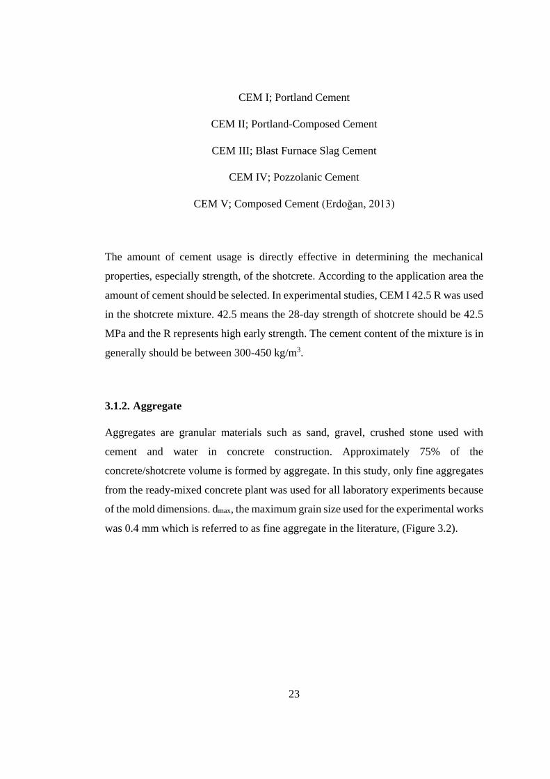
3.1.2. Aggregate
Aggregates are granular materials such as sand, gravel, crushed stone used with
cement and water in concrete construction. Approximately 75% of the
concrete/shotcrete volume is formed by aggregate. In this study, only fine aggregates
from the ready-mixed concrete plant was used for all laboratory experiments because
of the mold dimensions. dmax, the maximum grain size used for the experimental works
was 0.4 mm which is referred to as fine aggregate in the literature, (Figure 3.2).

24
Figure 3.2. Aggregate
According to the TS EN 1097-6 standard the density of aggregate for shotcrete-
concrete type of specimen should be between 2.5-3 g/cm3. Therefore, the pycnometer
test (Figure 3.3) was the precursor test that should be done in order to get specific
gravity of aggregates.
Pycnometer Test method and Calculation;
M1: mass of clean and dry empty pycnometer container
M2: mass of dry soil and pycnometer container together
M3: mass of dry soil and water mix with pycnometer container
M4: mass of pure water and pycnometer container
25
Figure 3.3. Pycnometer tests
The specific gravity of soil is determined using the relation below:
𝑀2−𝑀1
(𝑀2−𝑀1)−(𝑀3−𝑀4) (3.1)
Table 3.1. Pycnometer test parameters
𝑀1
(g)
𝑀2
(g)
𝑀3
(g)
𝑀4
(g)
G (Specific gravity of aggregate)
28.55 34.75 82.49 78.61 2.67
28.55 37.09 83.94 78.61 2.66
28.55 43.59 88.07 78.61 2.69
Average 2.68

26
3.1.3. Water
Water is used for two purposes. One of them is for washing aggregates to be used in
shotcrete, since aggregates may include clay, silt or organic materials that may
decrease surface adherence character of the pieces. The other one is for the preparation
of shotcrete mixture. Water and cement are combined in specified proportions to start
chemical reaction, namely hydration. Water and cement provide the desired
workability as fresh shotcrete mixture, following the washing of aggregate surfaces
and cement grains in the mixing process of shotcrete.
3.1.4. Admixtures/Additives
There are three purpose for using plasticizer, as an additive. The first one is by
reducing the water/cement ratio in the shotcrete mixture, it provides higher strength.
The second one is increasing the workability of fresh concrete without changing the
material quantities or proportion in the mixture. The third one is it provides technical
and economic benefits by keeping the water/cement ratio to be used in the mixture
constant, while reducing the water and cement quantities. The used admixture as
plasticizer is SIKA ViscoCrete Hi-Tech 2001, (Figure 3.4). The amount of plasticizer
should be 1% by weight of the cement amount.
Figure 3.4. Additives

27
3.2. 3D Molds and Recipe for Shotcrete
For fracture toughness testing work special molds of varying diameters were prepared.
SolidWorks software was used for the technical drawings of 3D-molds, (Figure 3.5).
The thickness/radius (t/R ratio) of the specimens was kept constant as 1.3 for all sizes.
Wall thickness and the solidity percentage of the molds were adjusted according to
the changing diameters in order to get high performance like resistance to the repeated
usage, and to prevent any damage to the sample during extraction out of the mold.
Figure 3.5. Drawing of FBD mold in SolidWorks
In Table 3.2, dimensions of the FBD specimens extracted from the 3D molds are
tabulated.

28
Table 3.2. Dimensions of the specimens extracted from the molds
Mold Name Diameter
(mm)
Thickness
(mm)
Height
(mm)
M-1
M-2
100
120
67
80
98
118
M-3 140 94 137
M-4 160 107 157
M-5 180 120 177
M-6 200 133 196
The picture of molds used for the investigation of size effect on fracture toughness test
is shown in Figure 3.6.
Figure 3.6. Used molds with varying diameters 100 mm to 200 mm
The 3D mold of each diameter group has its own mixture recipe which was adjusted
accordingly the volume of each mold and keeping recipe proportions the same. In
general, the recipe for shotcrete is expressed as for volume of 1dm3.

29
Recipe for 0.5 water/cement ratio shotcrete-concrete type of specimens for 1dm3
mixture;
Cement: 300 g
Water: 150 g
Aggregate: 2015 g
Admixture: 3 g
Recipe for all mold diameters were tabulated in Table 3.3 including the recipe for the
mold prepared specially for static deformability and Brazilian disc tests.
Table 3.3. Recipe for all diameters
Ingredient (g) Specimen Diameter (mm)
100 120 140 160 180 200
Cement 180 300 450 600 930 1260
Water 90 150 225 300 465 630
Admixture
(plasticizer) 1.8 3 4.5 6 9.3 12.6
Aggregates 1209 2015 3023 4030 6247 8463
Total Weight (g) 1480.8 2468 3702.5 4936 7651.3 10365.6
3.3. Preparation of Shotcrete Samples
For the preparation of the shotcrete samples, UTEST mixer with almost 10 dm3
capacity with adjustable speed was used, (Figure 3.7).
30
Figure 3.7. UTEST mixer
For the casting procedure, first, aggregate and then cement was put in the mixer and
materials were mixed for 40 seconds at slow speed in dry condition. After that the
liquid mixture was prepared including water and additive in it and poured into the dry
mixture. All materials were mixed at slow speed in first 40 seconds and then mixed
for 40 seconds in fast speed to achieve the homogeneity in the mixture. For each
sample, attention was given for the consistency and the homogeneity of the mixture.
As the shotcrete mixture design was set to the desired composition to get an early
strength, it was poured into molds without wasting any time. Before starting the
casting process, the molds were lubricated with motor oil in order to avoid difficulty
in demolding process, (Figure 3.8).
31
Figure 3.8. Lubrication process
During the casting procedure in order to avoid the air voids, vibration action was
needed and this was performed manually by hand shaking of the mixture in the mold,
(Figure 3.9).
Figure 3.9. Casted Shotcrete

32
Casting process is very important to obtain homogeneity. If the vibration process is
not performed well or nor done at all, layering occurs according to the casting order.
Homogeneity is disrupted by the formation of air voids in the upper side while the
remaining parts are well-settled on the bottom side, (Figure 3.10).
Figure 3.10. Successful and unsuccessful casting products
33
CHAPTER 4
4. TESTING FOR MECHANICAL PROPERTIES OF SHOTCRETE
Preparation of the shotcrete specimens were the first step for the conventional testing
work. Mix design were made according to the concrete-specification, performance,
production and conformity standard namely EN 206. Casting process was carried out
according to the specific geometry requirements of the particular tests. Cylindrical
core samples which had length/diameter of L/D=2.5 and D=70 mm were prepared for
static deformability tests. Cylindrical disc samples with thickness/diameter ratio of
t/D=0.5 were prepared for Brazilian Disc tests from the molds illustrated in Figure 4.1.
Figure 4.1. Prepared molds for conventional testing
34
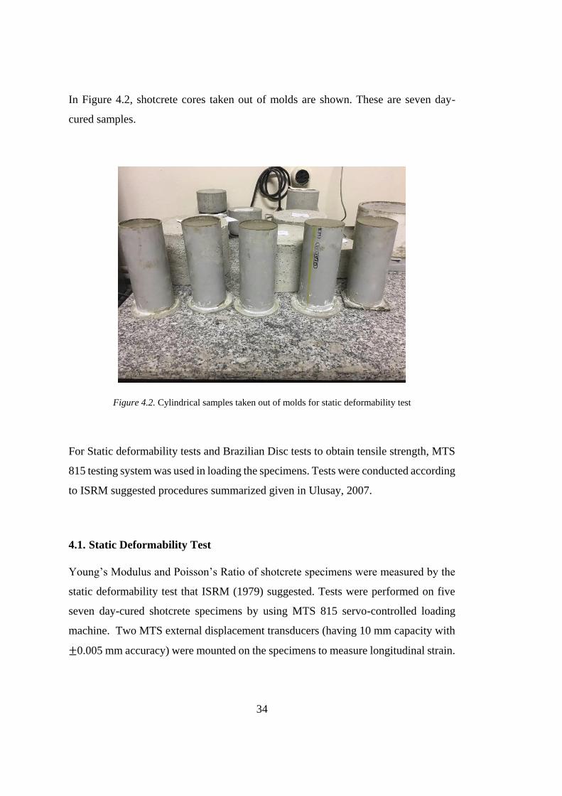
In Figure 4.2, shotcrete cores taken out of molds are shown. These are seven day-
cured samples.
Figure 4.2. Cylindrical samples taken out of molds for static deformability test
For Static deformability tests and Brazilian Disc tests to obtain tensile strength, MTS
815 testing system was used in loading the specimens. Tests were conducted according
to ISRM suggested procedures summarized given in Ulusay, 2007.
4.1. Static Deformability Test
Young’s Modulus and Poisson’s Ratio of shotcrete specimens were measured by the
static deformability test that ISRM (1979) suggested. Tests were performed on five
seven day-cured shotcrete specimens by using MTS 815 servo-controlled loading
machine. Two MTS external displacement transducers (having 10 mm capacity with
±0.005 mm accuracy) were mounted on the specimens to measure longitudinal strain.
35
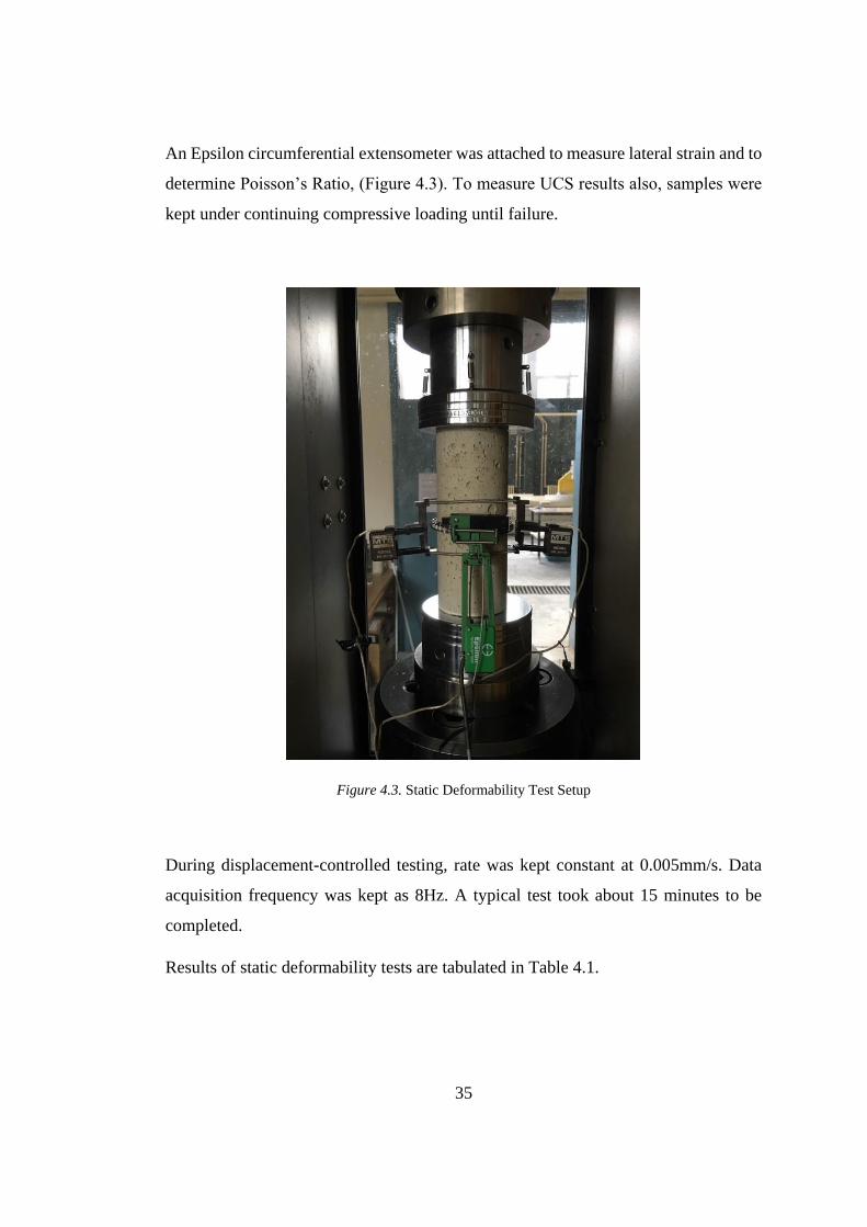
An Epsilon circumferential extensometer was attached to measure lateral strain and to
determine Poisson’s Ratio, (Figure 4.3). To measure UCS results also, samples were
kept under continuing compressive loading until failure.
Figure 4.3. Static Deformability Test Setup
During displacement-controlled testing, rate was kept constant at 0.005mm/s. Data
acquisition frequency was kept as 8Hz. A typical test took about 15 minutes to be
completed.
Results of static deformability tests are tabulated in Table 4.1.

36
Table 4.1. Static deformability test results
Specimen
Length
(mm)
Diameter
(mm)
UCS
(MPa)
Elastic
Modulus
(GPa)
Poisson's
Ratio
S_SD_1 177.5 71.4 25.9 20.03 0.18
S_SD_2 176.0 70.4 22.9 20.64 0.17
S_SD_3 173.5 71.0 29.7 20.96 0.18
S_SD_4 175.0 71.1 29.5 21.59 0.20
S_SD_5 175.0 70.4 24.8 23.81 0.18
Average
175.40 70.9 26.6±3.0 21.41±1.46 0.18±0.01
Average Uniaxial Compressive Strength (UCS) was calculated as 27 MPa. Elastic
Modulus (E) and Poisson’s Ratio (υ) were calculated as 21 GPa and 0.18, respectively.
A typical lateral strain- axial strain curve and stress-strain curve for shotcrete core
specimen are shown in Table 4.4 and Table 4.5, respectively.

37
Figure 4.4. Lateral strain vs axial strain graph
Figure 4.5. Stress vs lateral strain and axial strain graph
38
Test results presented in Table 4.1 are compared to some results reported in literature
to assess the representative shotcrete quality of the mixture used here.
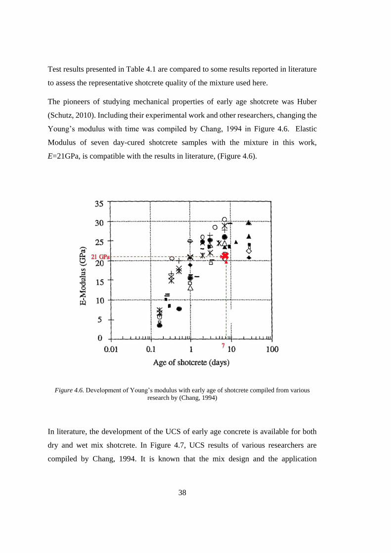
The pioneers of studying mechanical properties of early age shotcrete was Huber
(Schutz, 2010). Including their experimental work and other researchers, changing the
Young’s modulus with time was compiled by Chang, 1994 in Figure 4.6. Elastic
Modulus of seven day-cured shotcrete samples with the mixture in this work,
E=21GPa, is compatible with the results in literature, (Figure 4.6).
Figure 4.6. Development of Young’s modulus with early age of shotcrete compiled from various
research by (Chang, 1994)
In literature, the development of the UCS of early age concrete is available for both
dry and wet mix shotcrete. In Figure 4.7, UCS results of various researchers are
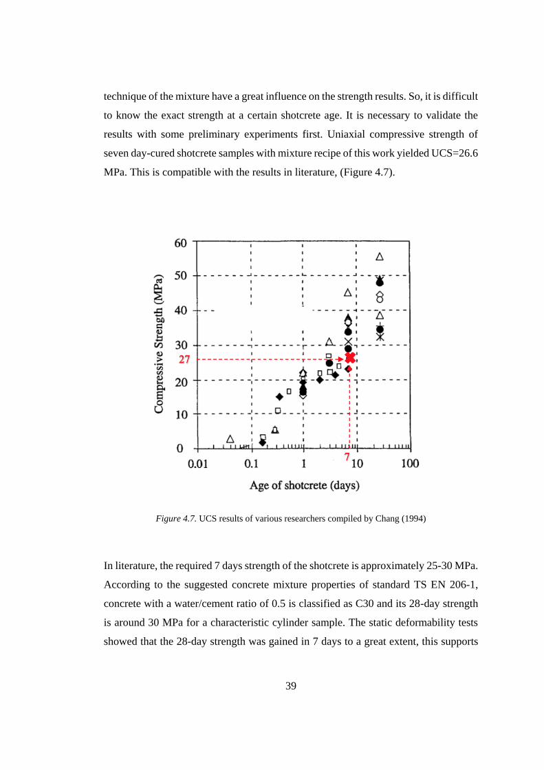
compiled by Chang, 1994. It is known that the mix design and the application
39
technique of the mixture have a great influence on the strength results. So, it is difficult
to know the exact strength at a certain shotcrete age. It is necessary to validate the
results with some preliminary experiments first. Uniaxial compressive strength of
seven day-cured shotcrete samples with mixture recipe of this work yielded UCS=26.6
MPa. This is compatible with the results in literature, (Figure 4.7).
Figure 4.7. UCS results of various researchers compiled by Chang (1994)
In literature, the required 7 days strength of the shotcrete is approximately 25-30 MPa.
According to the suggested concrete mixture properties of standard TS EN 206-1,
concrete with a water/cement ratio of 0.5 is classified as C30 and its 28-day strength
is around 30 MPa for a characteristic cylinder sample. The static deformability tests
showed that the 28-day strength was gained in 7 days to a great extent, this supports
40
the compatibility of the mixture prepared here to represent the shotcrete which is
aimed to provide high-early strength.
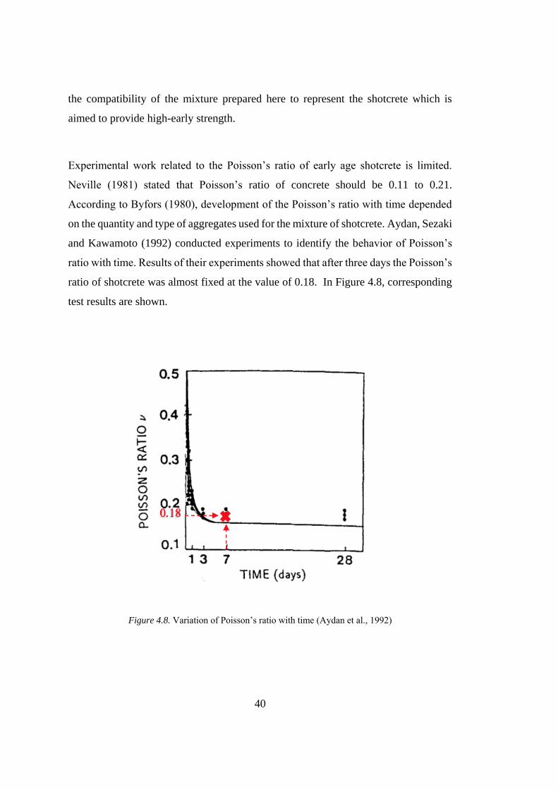
Experimental work related to the Poisson’s ratio of early age shotcrete is limited.
Neville (1981) stated that Poisson’s ratio of concrete should be 0.11 to 0.21.
According to Byfors (1980), development of the Poisson’s ratio with time depended
on the quantity and type of aggregates used for the mixture of shotcrete. Aydan, Sezaki
and Kawamoto (1992) conducted experiments to identify the behavior of Poisson’s
ratio with time. Results of their experiments showed that after three days the Poisson’s
ratio of shotcrete was almost fixed at the value of 0.18. In Figure 4.8, corresponding
test results are shown.
Figure 4.8. Variation of Poisson’s ratio with time (Aydan et al., 1992)
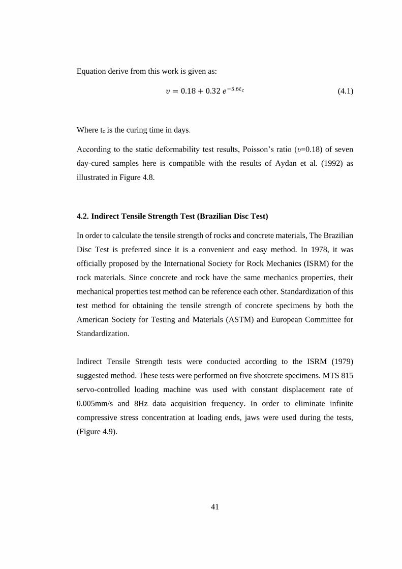
41
Equation derive from this work is given as:
𝜐 = 0.18 + 0.32 𝑒−5.6𝑡𝑐 (4.1)
Where tc is the curing time in days.
According to the static deformability test results, Poisson’s ratio (υ=0.18) of seven
day-cured samples here is compatible with the results of Aydan et al. (1992) as
illustrated in Figure 4.8.
4.2. Indirect Tensile Strength Test (Brazilian Disc Test)
In order to calculate the tensile strength of rocks and concrete materials, The Brazilian
Disc Test is preferred since it is a convenient and easy method. In 1978, it was
officially proposed by the International Society for Rock Mechanics (ISRM) for the
rock materials. Since concrete and rock have the same mechanics properties, their
mechanical properties test method can be reference each other. Standardization of this
test method for obtaining the tensile strength of concrete specimens by both the
American Society for Testing and Materials (ASTM) and European Committee for
Standardization.
Indirect Tensile Strength tests were conducted according to the ISRM (1979)
suggested method. These tests were performed on five shotcrete specimens. MTS 815
servo-controlled loading machine was used with constant displacement rate of
0.005mm/s and 8Hz data acquisition frequency. In order to eliminate infinite
compressive stress concentration at loading ends, jaws were used during the tests,
(Figure 4.9).

42
Figure 4.9. Brazilian Disc Test set up
In Table 4.2, Brazilian disc test results including peak loads and calculated tensile
strengths were tabulated, (Table 4.2). Diameter and thickness of all Brazilian Disc
specimens were around 71mm and 33 mm, respectively,
Table 4.2. Brazilian disc test results
Specimen
Name
Peak Load
(kN)
𝜎𝑡
(MPa)
S_BD_1 16.60 4.30
S_BD_2 17.89 4.60
S_BD_3 15.59 4.03
S_BD_4 14.45 3.66
S_BD_5 10.50 3.53
Average 15.01±2.82 4.02±0.44

43
According to the test results, the average peak load was 15 kN, and the average tensile
strength was calculated as σt = 4 MPa.
A typical Brazilian Disc Test sample namely S_BD_2 with central crack clearly
visible is shown in Figure 4.10.
Figure 4.10. A typical Brazilian Disc sample with central crack clearly visible
A typical force-displacement curve of the same specimen namely S_BD_2 during the
Indirect Tensile Strength Test with Brazilian Disc geometry is shown Figure 4.11.
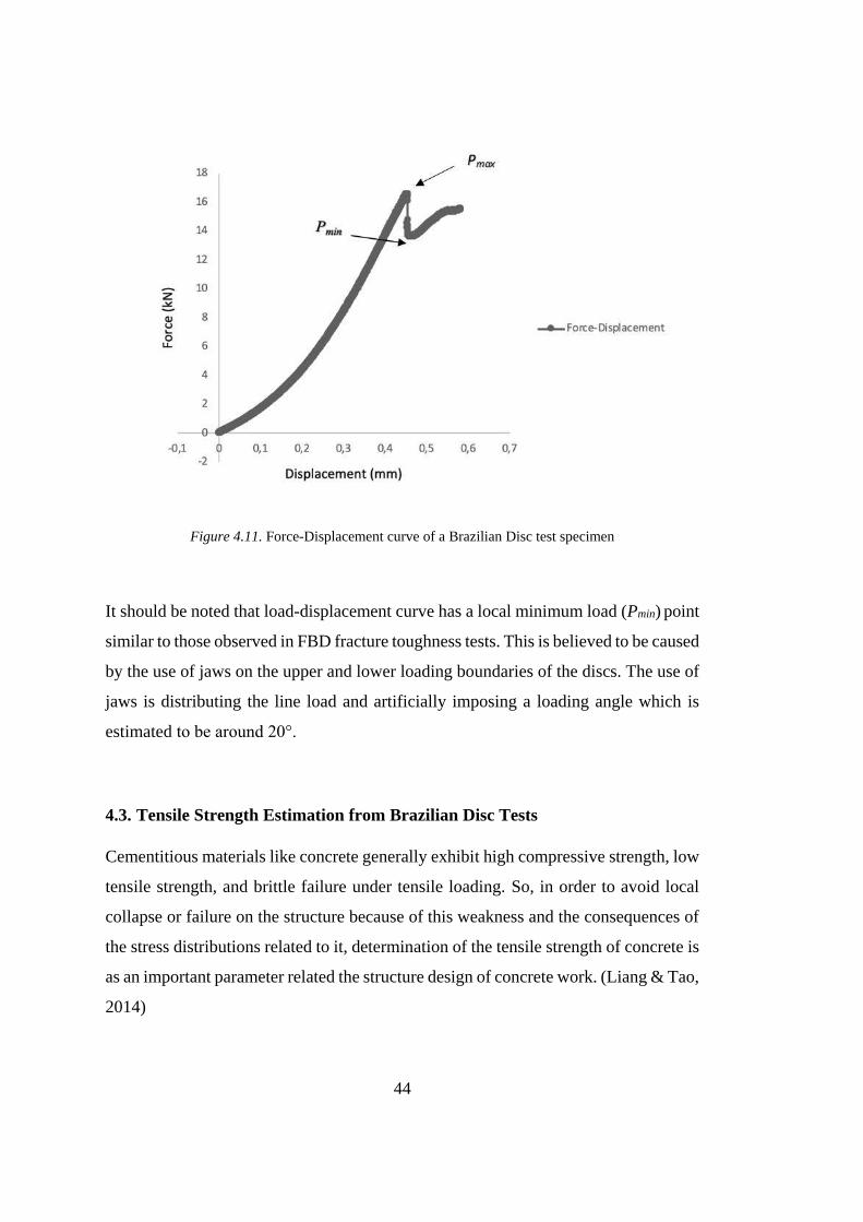
44
Figure 4.11. Force-Displacement curve of a Brazilian Disc test specimen
It should be noted that load-displacement curve has a local minimum load (Pmin) point
similar to those observed in FBD fracture toughness tests. This is believed to be caused
by the use of jaws on the upper and lower loading boundaries of the discs. The use of
jaws is distributing the line load and artificially imposing a loading angle which is
estimated to be around 20°.
4.3. Tensile Strength Estimation from Brazilian Disc Tests
Cementitious materials like concrete generally exhibit high compressive strength, low
tensile strength, and brittle failure under tensile loading. So, in order to avoid local
collapse or failure on the structure because of this weakness and the consequences of
the stress distributions related to it, determination of the tensile strength of concrete is
as an important parameter related the structure design of concrete work. (Liang & Tao,
2014)

45
It is possible to estimate tensile strength from FBD tests. Pmax values before the load
drop can be used in some recently developed expressions to compute tensile strength.
There are two well-known formulations for this purpose one is by Wang and the other
one is Keles and Tutluoglu. These are explained below.
4.3.1. Wang’s Approach
By assuming that the specimen is under uniformly distributed tensile stress, in 1953
Carneiro and Barcellos stated that the tensile strength can be expressed as:
𝜎𝑡 =2𝑃𝑚𝑎𝑥
𝜋𝐷𝑡 (4.2)
Where 𝜎𝑇 is tensile strength, 𝑃𝑚𝑎𝑥 is the failure load of the specimen, D is the diameter
of the specimen, t is the thickness of the specimen, (Japaridze, 2015).
However, the Brazilian test has the disadvantage that high shear stresses are induced
close to the loading platens apart from the tensile stresses, which are developed in the
disc. Wang and Xing (1999) introduced two mutually parallel planes to be used as
surface loading application to the disc. Parallel loading ends are used to distribute the
concentrated load. Griffith strength criterion (Griffith, 1924) was applied by Wang
and Xing (1999); Wang and Wu (2004); Wang, Jia, Kou, Zhang and Lindqvist
(2004a); Kaklis, Agioutantis, Sarris and Pateli (2005) and Keles & Tutluoglu (2011)
to develop an analytical formula to calculate the tensile strength in Flattened Brazilian
Disc.
According to the Griffith’s theory to form cracks at the center in regular Brazilian test
stress conditions required are;
3𝜎1 + 𝜎3 = 0 Which yields, 𝜎𝐺 = 2𝑃
𝜋𝐷𝑡 (4.3)

46
Where 𝜎1 and 𝜎3 are maximum principle stress and minimum principle stress,
respectively at the center. 𝜎𝐺 = 𝜎𝜃 at the same time.
The failure occurs, 𝜎𝑡 = 𝜎𝐺 where 𝜎𝐺the equivalent stress is, and it was based on the
principle stresses 𝜎1 maximum and 𝜎3 minimum and if the tensile stress is considered
positive:
If 3𝜎1 + 𝜎3 ≥ 0 , then 𝜎1 = 𝜎𝑡 (4.4)
If 3𝜎1 + 𝜎3 < 0 , then 𝜎𝐺 = 𝜎𝑡 = −(𝜎1−𝜎3)2
8(𝜎1+𝜎3) (4.5)
In cylindrical system, the stress inside the sample can be expressed by 𝜎𝜃 and 𝜎𝑟
.Wang et al. (2004) assumed that there is no shear stress in the direction of 𝜎𝜃 and 𝜎𝑟.
Timoshenko and Goodier (1970) stated that when a Brazilian disc is subjected to a
radial compressive force, the stress solution on the loading diameter can be expressed
as:
𝜎𝜃 =2𝑃
𝜋𝐷𝑡 (4.6)
𝜎𝑟 =2𝑃
𝜋𝐷𝑡 (1 −
4𝐷2
𝐷2−4𝑟2) (4.7)
When the Brazilian Disc is flattened loading angle comes into the problem. Wang et
al. (2004) analyzed the crack initiation condition at the center and they stated that
when 2α is equal or larger than 20°, the primary tensile crack will initiate at the center
and 𝜎𝐺 must reach a maximum value at that point.
Thus, for the Flattened Brazilian Disc at the center of disc;

47
(𝜎𝑟−𝜎𝜃)2
8(𝜎𝑟+𝜎𝜃)= 𝜎𝐺 = 𝜎𝑡 (4.8)
To determine 𝜎𝑇, Wang et al. (2004) derived approximate formulae for 𝜎𝜃 and 𝜎𝑟 and
they assumed that the crack initiates at the specimen center, (Figure 4.12).
Figure 4.12. Specimen subjected to a uniform diametric loading (Wang et al.,2004)
𝜎𝜃 = −2𝑃
𝜋𝐷𝑡 𝑐𝑜𝑠3𝛼
𝛼
𝑠𝑖𝑛𝛼 (4.9)
𝜎𝑟 =2𝑃
𝜋𝐷𝑡 (𝑐𝑜𝑠3𝛼 + 𝑐𝑜𝑠𝛼 +
𝑠𝑖𝑛𝛼
𝛼)
𝛼
𝑠𝑖𝑛𝛼 (4.10)
Wang et al. (2004) expressed 𝜎𝑡 as:
𝜎𝑡 =2𝑃
𝜋𝐷𝑡[
(2𝑐𝑜𝑠3𝛼+𝑐𝑜𝑠𝛼+𝑠𝑖𝑛𝛼𝑠⁄ )
2
8(𝑐𝑜𝑠𝛼+𝑠𝑖𝑛𝛼𝛼⁄ )
𝛼
𝑠𝑖𝑛𝛼] (4.11)
k

48
So, In Flattened Brazilian Disc, a dimensionless correction coefficient k is joined to
the equation to determine tensile strength formula.
𝜎𝑡 = 𝑘2𝑃𝑚𝑎𝑥
𝜋𝐷𝑡 (4.12)
In order to get tensile strength from flattened Brazilian disc geometry, correction
coefficient k is calculated from Wang’s equation for loading angle of 2α=22° (0.19
radian) and the result was equal to k= 0.9522.
By using k into the equation and also Flattened Brazilian disc specimens’ failure loads
(Pmax), diameters (D), thickness (t), indirect tensile strength for changing diameters
between 100 mm to 200mm at constant loading angle was calculated. In Table 4.3,
calculated tensile strength and the geometric parameters of the specimens were
tabulated. The tensile strength values computed as the average of five tests.
Table 4.3. Average tensile strength from Wang’s correction coefficient
Group
Name
Dave
(mm)
tave
(mm)
Pmax ave
(kN)
𝜎𝑡 𝑊
(MPa)
S100 99.0 66.62 24.98 2.30
S120 118.5 79.55 37.31 2.40
S140 138.4 83.99 45.77 2.39
S160 158.1 103.86 67.68 2.50
S180 174.4 122.38 102.92 2.87
S200 197.6 133.16 127.14 2.93
∗ 𝜎𝑡 𝑊 represents calculated tensile strength by using Wang’s correction coefficient.
The change in tensile strength with the specimen diameter is shown in Figure 4.13.
Tensile strength increases with sample size following a fitted third degree polynomial.
The lowest 2.30 for 100 mm size group and the highest is 2.87 for the 200 mm group.
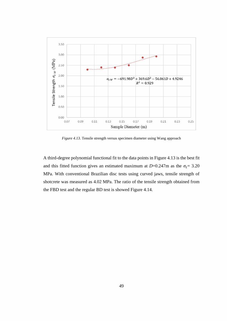
49
Figure 4.13. Tensile strength versus specimen diameter using Wang approach
A third-degree polynomial functional fit to the data points in Figure 4.13 is the best fit
and this fitted function gives an estimated maximum at D=0.247m as the 𝜎𝑡= 3.20
MPa. With conventional Brazilian disc tests using curved jaws, tensile strength of
shotcrete was measured as 4.02 MPa. The ratio of the tensile strength obtained from
the FBD test and the regular BD test is showed Figure 4.14.
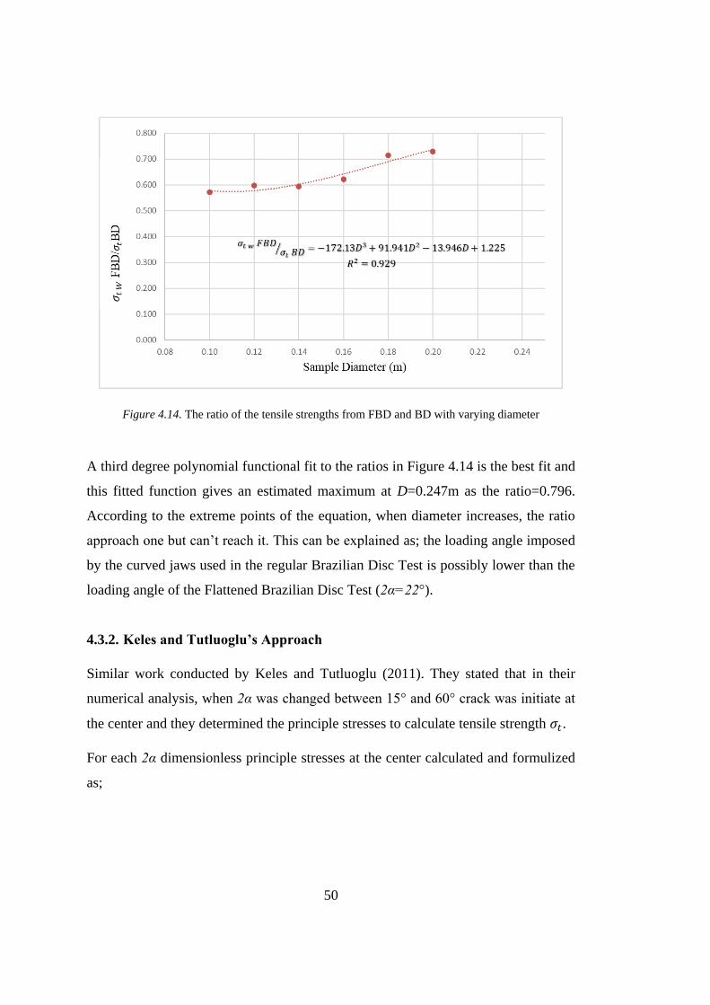
50
Figure 4.14. The ratio of the tensile strengths from FBD and BD with varying diameter
A third degree polynomial functional fit to the ratios in Figure 4.14 is the best fit and
this fitted function gives an estimated maximum at D=0.247m as the ratio=0.796.
According to the extreme points of the equation, when diameter increases, the ratio
approach one but can’t reach it. This can be explained as; the loading angle imposed
by the curved jaws used in the regular Brazilian Disc Test is possibly lower than the
loading angle of the Flattened Brazilian Disc Test (2α=22°).
4.3.2. Keles and Tutluoglu’s Approach
Similar work conducted by Keles and Tutluoglu (2011). They stated that in their
numerical analysis, when 2α was changed between 15° and 60° crack was initiate at
the center and they determined the principle stresses to calculate tensile strength 𝜎𝑡.
For each 2α dimensionless principle stresses at the center calculated and formulized
as;
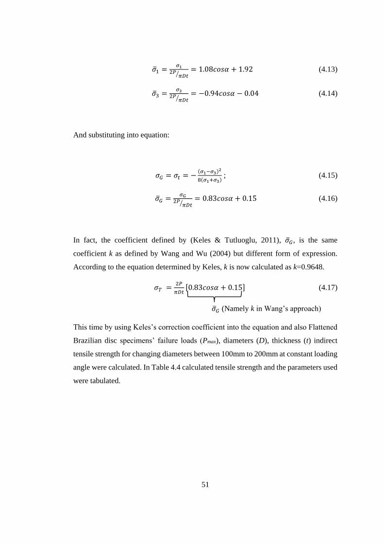
51
�̅�1 =𝜎1
2𝑃𝜋𝐷𝑡⁄
= 1.08𝑐𝑜𝑠𝛼 + 1.92 (4.13)
�̅�3 =𝜎3
2𝑃𝜋𝐷𝑡⁄
= −0.94𝑐𝑜𝑠𝛼 − 0.04 (4.14)
And substituting into equation:
𝜎𝐺 = 𝜎𝑡 = −(𝜎1−𝜎3)2
8(𝜎1+𝜎3) ; (4.15)
�̅�𝐺 =𝜎𝐺
2𝑃𝜋𝐷𝑡⁄
= 0.83𝑐𝑜𝑠𝛼 + 0.15 (4.16)
In fact, the coefficient defined by (Keles & Tutluoglu, 2011), �̅�𝐺, is the same
coefficient k as defined by Wang and Wu (2004) but different form of expression.
According to the equation determined by Keles, k is now calculated as k=0.9648.
𝜎𝑇 =2𝑃
𝜋𝐷𝑡[0.83𝑐𝑜𝑠𝛼 + 0.15] (4.17)
�̅�𝐺 (Namely k in Wang’s approach)
This time by using Keles’s correction coefficient into the equation and also Flattened
Brazilian disc specimens’ failure loads (Pmax), diameters (D), thickness (t) indirect
tensile strength for changing diameters between 100mm to 200mm at constant loading
angle were calculated. In Table 4.4 calculated tensile strength and the parameters used
were tabulated.
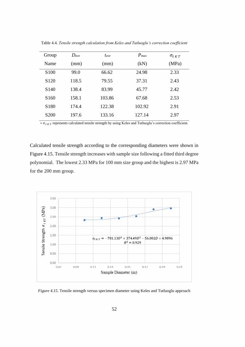
52
Table 4.4. Tensile strength calculation from Keles and Tutluoglu’s correction coefficient
Group
Name
Dave
(mm)
tave
(mm)
Pmax
(kN)
𝜎𝑡 𝐾 𝑇
(MPa)
S100 99.0 66.62 24.98 2.33
S120 118.5 79.55 37.31 2.43
S140 138.4 83.99 45.77 2.42
S160 158.1 103.86 67.68 2.53
S180 174.4 122.38 102.92 2.91
S200 197.6 133.16 127.14 2.97
∗ 𝜎 𝑡 𝐾 𝑇 represents calculated tensile strength by using Keles and Tutluoglu’s correction coefficient.
Calculated tensile strength according to the corresponding diameters were shown in
Figure 4.15. Tensile strength increases with sample size following a fitted third degree
polynomial. The lowest 2.33 MPa for 100 mm size group and the highest is 2.97 MPa
for the 200 mm group.
Figure 4.15. Tensile strength versus specimen diameter using Keles and Tutluoglu approach
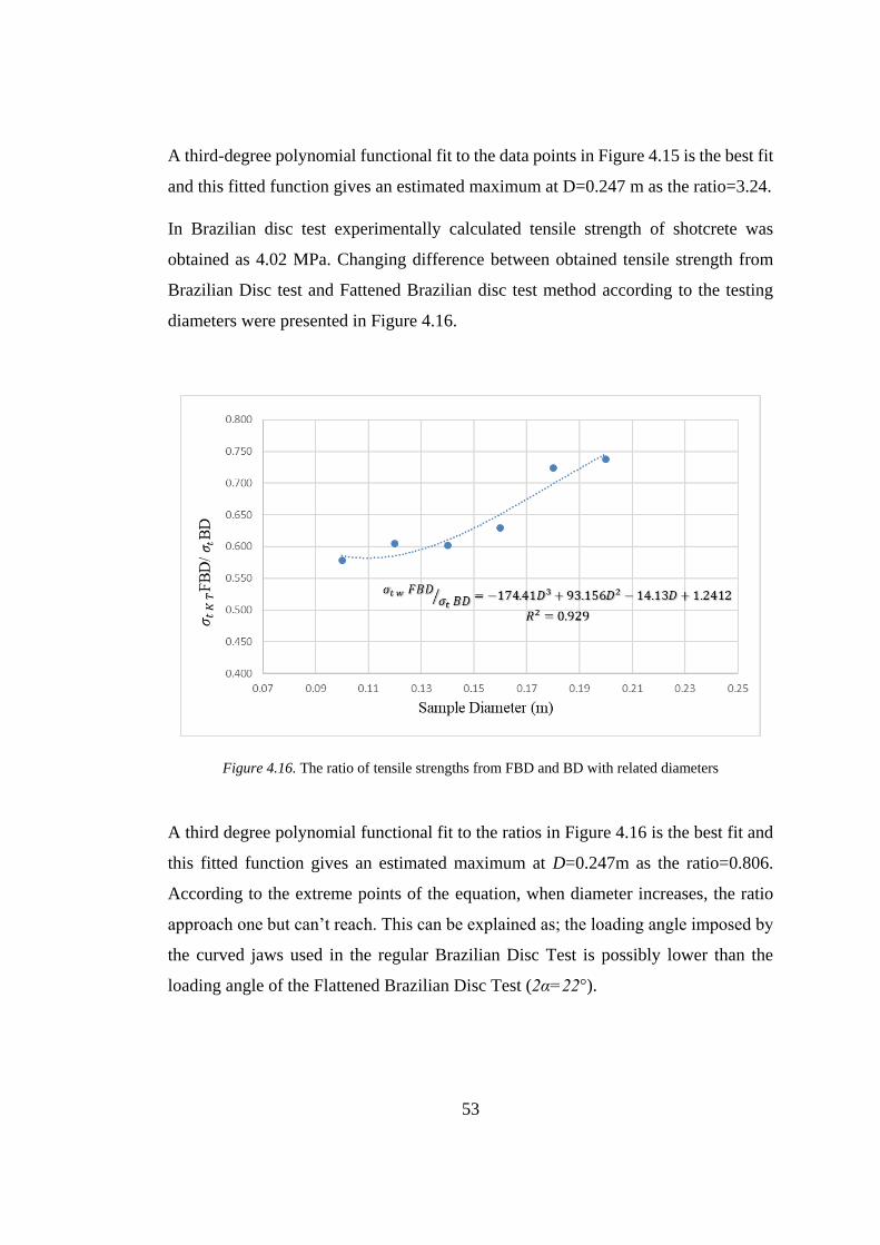
53
A third-degree polynomial functional fit to the data points in Figure 4.15 is the best fit
and this fitted function gives an estimated maximum at D=0.247 m as the ratio=3.24.
In Brazilian disc test experimentally calculated tensile strength of shotcrete was
obtained as 4.02 MPa. Changing difference between obtained tensile strength from
Brazilian Disc test and Fattened Brazilian disc test method according to the testing
diameters were presented in Figure 4.16.
Figure 4.16. The ratio of tensile strengths from FBD and BD with related diameters
A third degree polynomial functional fit to the ratios in Figure 4.16 is the best fit and
this fitted function gives an estimated maximum at D=0.247m as the ratio=0.806.
According to the extreme points of the equation, when diameter increases, the ratio
approach one but can’t reach. This can be explained as; the loading angle imposed by
the curved jaws used in the regular Brazilian Disc Test is possibly lower than the
loading angle of the Flattened Brazilian Disc Test (2α=22°).

54
Figure 4.17. Bazant’s size effect investigation (Bazant et al., 1991)
According to Bazant's study, for the small sizes, the Brazilian Disc strength decreased
with increasing size until a certain diameter. As a result of experiments applied in
concrete while diameter of the specimen changed from 10 to 508 mm, threshold
diameter was around 200 mm. After that certain diameter, strength increased in direct
proportion. In this study, for the shotcrete specimens that had 0.5 water/cement ratio,
the increasing behavior of tensile with diameter was observed between 100 mm
diameter and 200 mm diameter.
55
CHAPTER 5
5. MODE I FRACTURE TOUGHNESS TESTS
Understanding the fracture mechanism is crucial to solve many engineering problems.
In order to be able to investigate the conditions of the fracture growth, measurement
of toughness is required for fracture analysis.
When considered the other testing methods, Flattened Brazilian Disc Test method has
been preferred testing method for determination of the fracture toughness due to the
relatively easiness for the specimen preparation, compressive load application on the
flat ends and also simple testing procedure.
For fracture toughness testing, FBD method with flat compressive load application
boundaries is the simplest method among the other methods considering specimen
preparation, loading type, and testing procedures.
Objective of this work is to study the variation fracture toughness of shotcrete with
specimen size and curing time. 30 experiments were performed to investigate the size
effect on mode I fracture toughness and 21 experiments were performed to investigate
the effect of curing time on mode I fracture toughness.
5.1. Fracture Toughness Testing Work
Before conducting the experiments, dimensions of the specimens were measured since
all of the specimens differed slightly due to the imperfections of casting process.
Shotcrete specimens were prepared with six different diameters which are 100 mm,
120 mm, 140 mm, 160 mm, 180 mm, and 200 mm.

56
In the second part of the experimental program effect of curing time on KIC was
investigated by varying the curing time tc as 1 day, 2 days, 3 days, 5 days and 7 days.
For a specific diameter of 160 mm, they were grouped depending on the five curing
time levels in order to investigate the curing time effect on the fracture toughness of
the shotcrete.
During all the tests, specimens were loaded using the MTS 815 servo-controlled
loading machine with a constant displacement rate of 0.0004 mm/s and 8Hz data
acquisition frequency.
In all fracture toughness testing work, loading angle 2α of the specimens is kept nearly
as 22° which corresponds to flattened end/radius ratio of L/R=0.19.
When the experiment started, load gradually increased up to a maximum point, Pmax
at which an unstable crack initiated at the center of the specimen. At this stage, a
sudden drop in load from Pmax to local minimum, Pmin occurred. Local minimum
point, Pmin was the turning point between unstable and to stable crack propagation.
Stable crack growth started at the Pmin. At this load, experimental critical crack length
(ace) was measured. Close-up photos were taken in order to measure the critical crack
lengths through Adobe Photoshop Program. The purpose was the comparison between
experimental and numeric critical crack lengths. Specimen dimensions, Pmax, Pmin and
experimental critical crack length were recorded for each test. The average of the
recorded Pmax values of each testing group was used for the tensile strength
computations from FBD geometry with the help of two researcher’s approaches.
A typical force-displacement curve related the Mode I Fracture Toughness Test with
Flattened Brazilian Disc geometry is shown Figure 5.1.

57
Figure 5.1. A typical Force-Displacement curve of a Flattened Brazilian Disc test
According to the Wang and Wu (2004), the last discussion was about the validity of a
FBD test. To be valid, the failure must be caused by the development of the primary
crack, not the secondary ones. In a typical force displacement graph of the test results,
when the load reaches the maximum (Pmax) at the end of elastic deformation, and local
minimum load (Pmin) is reached when the primary cracks propagate till its critical
length. Second increase in load must be observed to progress up to a load level which
is supposed to be lower than Pmax. The load increase in the second rise should never
be greater than the first one, (Figure 5.1). Otherwise, the secondary cracks would play
role in the failure and disc may be split into more pieces than it should be. This
criterion was taken into consideration in all the testing work here.

58
A typical experimental critical crack length measurement related the Mode I Fracture
Toughness Test with Flattened Brazilian Disc geometry is shown Figure 5.2.
Figure 5.2. A typical experimental critical crack length measurement
5.2. Computation for Fracture Toughness
For determining the mode I fracture toughness value for FBD testing method was
calculated by using the Eq. 5.1 (Wang and Xing, 1999).
𝐾𝐼𝑐 =𝑌𝐼𝑚𝑎𝑥 𝑃𝑚𝑖𝑛
𝑡 √𝑅 (5.1)
Where,
𝐾𝐼𝑐 : Fracture toughness (MPa√𝑚)
Pmin : Minimum local load (kN)

59
R : Specimen Radius (mm)
t : Specimen thickness (mm)
𝑌𝐼𝑚𝑎𝑥 : Maximum dimensionless stress intensity factor (SIF) which is determined
from numerical modeling.
Özdoğan (2017) developed a formula based on numerical analysis for determination
of the critical crack length and the maximum dimensionless stress intensity factor at
the onset of stable crack propagation or at the local minimum points depending on the
loading angle. The J-integral approach was used for KI computation in ABAQUS
models.
Özdoğan followed a procedure that numerical FBD models were developed based on
different dimensionless crack lengths (a/R) for each loading angle in order to find KI
values. The KI values obtained from these models were converted into YI values by
using the equation described by Wang and Xing (1999) as follows;
𝑌𝐼 =𝐾𝐼 𝑡 √𝑅
𝑃 (5.2)
Between the range of loading angles 2 to 50, numerical models of FBD were created
based on different dimensionless crack lengths (a/R) in order to find mode I stress
intensity factor (KI) values. KI values from the ABAQUS were used to calculate
dimensionless stress intensity factor YI by Wang’s formula. For each loading angle,
a/R depended YI values were fitted graphs and YImax values were generated by using
statistical program packages. There were two equations generated; one was for finding
YImax values for each loading angle, (Özdoğan,2017):
𝑌𝐼𝑚𝑎𝑥= 𝑒
1.6897+1.4854∗(2)−62.3324∗(2)2
1+31.7876∗(2)+4.3693∗(2)2−2.1703∗(2)3 (5.3)

60
In the Eq. (5.3), YImax represents maximum mode I dimensionless stress intensity factor
(SIF) and 2α is loading angle in radians.
The second equation fitted on acn/R vs loading angle (2α) plot and generated a formula
given in Eq. (5.4), (Özdoğan,2017):
𝑎𝑐𝑛𝑅⁄ =0.9974*e-0.844*(2) (5.4)
In Eq. (5.4), loading angle, 2α is in radians.
According to Özdoğan (2017), these equations are valid and reliable for loading angles
(2α) between 2 to 50. However, while working on the Brazilian test theoretically,
experimentally and numerically the validity of such tests needed to be investigated by
paying attention to the crack initiation location. In literature, there were many
investigations of the stress analyses for crack initiation location on Brazilian disc such
as studies of Wang and Xing (1999); Wang and Wu (2004); Wang et al. (2004a);
Kaklis et al. (2005) and Keles and Tutluoglu (2011). By using boundary element
method, critical 2α was found to be greater than 19.5° (Wang and Xing 1999). This
angle was found to be equal to 20° and Wang and Wu (2004) and Wang et al. (2004a),
reported that the upper limit for this angle should not be too large. It was 15° in Kaklis
et al. (2005) while it was between 15° to 60° in Keles and Tutluoglu (2011) by finite
element methods.
Considering the suggestions in the literature and practicality of constructing molds,
loading angle 2α was selected as 22° in current work, so that crack is expected to
initiate and develop along the central path.
According to the selected loading angle 2α=22° which was 0.384 in radians
corresponding YImax was calculated mathematically as 0.604 for all diameters.

61
After finding YImax for tested specimens numerically, for determining the mode I
fracture toughness value for FBD testing method was calculated by using the Eq. (5.5)
𝐾𝐼𝑐 =𝑌𝐼𝑚𝑎𝑥 𝑃𝑚𝑖𝑛
𝑡 √𝑅 (5.5)
For loading angle of 22° (0.384 in radians), corresponding acn/R was calculated
mathematically as 0.721. For each sample diameter, the measured critical crack length
at the local minimum point and numerically computed critical crack length for 2α=22°
loading angle were compared in proceeding sections.
5.3. Investigation of Size Effect on Mode I Fracture Toughness of Shotcrete
Size effect is an important characteristic of the fracture behavior in quasi brittle
materials such as concretes, rocks and ceramics. The strength and toughness of
specimens or structures made of these materials depends on their size thus especially
in the field of engineering applications, using fracture mechanics is the most
challenging concept to investigate.
The size effect was described as the geometrically similar structures have different
nominal stress with respect to varying sizes. Perdikaris, Calomino and Chudnovsky
(1986) indicated that the observed size effect on the fracture toughness in the static
and fatigue tests suggested that GIC and KIC cannot be considered to be material
parameters, (Perdikaris, 1986).
Bazant et al. (1991) conducted experimental studies to investigate the size effect on
Brazilian concrete specimens and he deduced that up to a certain critical diameter, size
effect existed and crack length expanded.
62
In this study while working with specimen size, loading angle kept constant at 22° in
order to observe the effect of different diameters on mode I fracture toughness.
Shotcrete-concrete FBD testing specimens were prepared according to six different
diameters which are 100 mm, 120 mm, 140 mm, 160 mm, 180 mm, and 200 mm. A
total of 30 experiments were performed to investigate the size effect on mode I fracture
toughness; that is approximately 5 experiments of each diameter group.
Test specimens’ name code was explained below Figure 5.3. Code includes type of
specimen, sample diameter (D), and the number of testing specimen, (Figure 5.3).
Figure 5.3. Name code of tested FBD specimens
A typical Flattened Brazilian Disc Test geometry with generalized dimensions was
shown in Figure 5.4 .

63
Figure 5.4. FBD specimen geometry
General geometric entities of the diameter-based specimen groups related to their
codes are given in Table 5.1.
Table 5.1. Dimensions of shotcrete specimens
Name D (mm) 2L(mm) t (mm)
S100 100 19 67
S120 120 23 80
S140 140 27 84
S160 160 31 104
S180 180 34 122
S200 200 38 133

64
5.3.1. Tables for Individual Fracture Toughness Test Results
Individual test results are presented in Tables 5.2 to 5.7 for the seven day-cured
samples of 100 mm, 120 mm, 140 mm, 160 mm, 180 mm and 200 mm diameter
groups.
Table 5.2. t, 2ace, ace/R, Pmin, and KIC values of FBD specimens having 100 mm diameter
Name t(mm) 2ace(mm) ace/R Pmin(kN) 𝐾𝐼𝐶(𝑀𝑃𝑎√𝑚 )
S100_s1 66.1 71.3 0.720 24.63 1.01
S100_s2 66.0 71.6 0.723 25.03 1.03
S100_s3 71.9 71.5 0.723 20.15 0.76
S100_s4 67.2 71.6 0.723 21.98 0.89
S100_s5 62.1 71.5 0.722 21.94 0.96
Average 71.5±0.12 22.75±2.05 0.93±0.11
Table 5.3. t, 2ace, ace/R, Pmin, and KIC values of FBD specimens having 120 mm diameter
Name t(mm) 2ace(mm) ace/R Pmin(kN) 𝐾𝐼𝐶(𝑀𝑃𝑎√𝑚 )
S120_s1 80.5 84.4 0.712 32.34 1.00
S120_s2 81.7 84.8 0.716 32.64 0.99
S120_s3 79.2 85.1 0.716 28.13 0.88
S120_s4 79.1 86.3 0.730 34.43 1.08
S120_s5 79.1 86.5 0.730 27.40 0.86
S120_s6 77.7 86.3 0.730 33.71 1.08
Average 85.6±0.91 31.44±2.95 0.98±0.09
Table 5.4. t, 2ace, ace/R, Pmin, and KIC values of FBD specimens having 140 mm diameter
Name t(mm) 2ace(mm) ace/R Pmin(kN) 𝐾𝐼𝐶(𝑀𝑃𝑎√𝑚 )
S140_s1 77.9 100.6 0.727 37.14 1.09
S140_s2 80.2 102.2 0.736 38.65 1.11
S140_s3 94.3 101.9 0.738 47.47 1.16
S140_s4 78.5 99.5 0.719 32.65 0.96
S140_s5 89.1 101.0 0.731 38.99 1.01
Average 101.0±1.08 38.98±5.38 1.06±0.08

65
Table 5.5. t, 2ace, ace/R, Pmin, and KIC values of FBD specimens having 160 mm diameter
Name t(mm) 2ace(mm) ace/R Pmin(kN) 𝐾𝐼𝐶(𝑀𝑃𝑎√𝑚 )
S160_s1 104.3 114.1 0.722 57.85 1.19
S160_s2 105.4 115.7 0.732 57.04 1.16
S160_s3 104.9 114.4 0.722 56.28 1.15
S160_s4 102.0 116.0 0.734 57.96 1.22
S160_s5 102.8 115.5 0.729 56.54 1.18
Average 115.1±0.84 57.13±0.76 1.18±0.03
Table 5.6. t, 2ace, ace/R, Pmin, and KIC values of FBD specimens having 180 mm diameter
Name t(mm) 2ace(mm) ace/R Pmin(kN) 𝐾𝐼𝐶(𝑀𝑃𝑎√𝑚 )
S180_s1 121.7 130.8 0.743 85.69 1.43
S180_s2 124.1 129.2 0.726 88.00 1.44
S180_s3 123.4 131.4 0.739 88.83 1.46
S180_s4 123.1 131.5 0.739 88.71 1.46
S180_s5 119.6 131.2 0.741 81.20 1.38
Average 130.8±0.94 86.49±3.21 1.43±0.03
Table 5.7. t, 2ace, ace/R, Pmin, and KIC values of FBD specimens having 200 mm diameter
Name t(mm) 2ace(mm) ace/R Pmin(kN) 𝐾𝐼𝐶(𝑀𝑃𝑎√𝑚 )
S200_s1 136.7 150.4 0.760 114.11 1.60
S200_s2 132.0 147.8 0.748 97.18 1.42
S200_s3 131.9 149.3 0.756 95.81 1.40
S200_s4 132.0 148.4 0.751 99.28 1.45
Average 149.0±1.13 101.60±8.46 1.46±0.09
KIC is seen to increase significantly with specimen size. The increase in KIC is almost
57% from 100 mm to 200 mm.

66
5.4. Investigation of Curing Time on Mode I Fracture Toughness of
Shotcrete/Concrete Type of Specimen
In order to investigate the effects of curing time on fracture toughness of shotcrete-
concrete type of specimen, 1 day, 2 days, 3 days, 5 days and 7 days air-cured shotcrete
specimens were tested. Diameter and the loading angle was kept constant at 160 mm
and 22°, respectively. A total of 21 experiment results were investigated to analyze
the effect of curing time on mode I fracture toughness of shotcrete specimens. For
each curing time investigation group, four tests were conducted.
It can be discussed that the crack propagation mechanism developed for mature
concrete can be applied to the early aged concrete (Hillerborg et al., 1976; Bazant,
2002). However, process of propagation cannot be fully explained by using this
approach. (Dao, Dux, and Morris, 2014).
Test specimens’ name code was explained below Figure 5.3. Code includes type of
specimen, sample diameter (D), curing time (day) and the number of testing specimen,
(Figure 5.5).
Figure 5.5. Name code of tested FBD specimens

67
5.4.1. Tables of Results for Curing Time Investigation
In Tables 5.8 to 5.12, KIC values are listed for 1 day, 2 day, 3 day, 5 day and 7 day air-
cured of 160 mm diameter samples. For seven-day cured 160 mm diameter group,
additional result was available from the size effect study.
Table 5.8. t, Pmin, and KIC values of FBD specimens having 160 mm diameter with 1 day cured
Name t(mm) Pmin(kN) 𝐾𝐼𝐶(𝑀𝑃𝑎√𝑚 )
S160-1D-s1 103.8 33.20 0.69
S160-1D-s2 104.7 29.42 0.60
S160-1D-s3 104.3 31.38 0.65
S1601-D-s5 104.0 33.29 0.69
Average 31.82±1.83 0.66±0.04
Table 5.9. t, Pmin, and KIC values of FBD specimens having 160 mm diameter with 2 days cured
Name t(mm) Pmin(kN) 𝐾𝐼𝐶(𝑀𝑃𝑎√𝑚 )
S160-2D-s1 104.0 37.28 0.77
S160-2D-s2 105.0 42.28 0.87
S160-2D-s3 104.4 36.36 0.75
S160-2D-s4 103.0 38.85 0.81
Average 38.69±2.60 0.80±0.05
Table 5.10. t, Pmin, and KIC values of FBD specimens having 160 mm diameter with 3 days cured
Name t(mm) Pmin(kN) 𝐾𝐼𝐶(𝑀𝑃𝑎√𝑚 )
S160-3D-s1 103.9 38.60 0.80
S160-3D-s2 104.5 39.94 0.82
S160-3D-s3 103.8 42.28 0.88
S160-3D-s4 104.0 40.80 0.84
Average 40.41±1.54 0.83±0.03
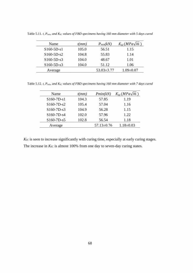
68
Table 5.11. t, Pmin, and KIC values of FBD specimens having 160 mm diameter with 5 days cured
Name t(mm) Pmin(kN) 𝐾𝐼𝐶(𝑀𝑃𝑎√𝑚 )
S160-5D-s1 105.0 56.51 1.15
S160-5D-s2 104.8 55.83 1.14
S160-5D-s3 104.0 48.67 1.01
S160-5D-s3 104.0 51.12 1.06
Average 53.03±3.77 1.09±0.07
Table 5.12. t, Pmin, and KIC values of FBD specimens having 160 mm diameter with 7 days cured
Name t(mm) Pmin(kN) 𝐾𝐼𝐶(𝑀𝑃𝑎√𝑚 )
S160-7D-s1 104.3 57.85 1.19
S160-7D-s2 105.4 57.04 1.16
S160-7D-s3 104.9 56.28 1.15
S160-7D-s4 102.0 57.96 1.22
S160-7D-s5 102.8 56.54 1.18
Average 57.13±0.76 1.18±0.03
KIC is seen to increase significantly with curing time, especially at early curing stages.
The increase in KIC is almost 100% from one day to seven-day curing states.

69
CHAPTER 6
6. EXPERIMENTAL RESULTS AND DISCUSSION
Tests with Flattened Brazilian Disc geometry were carried out to detect the presence
of size effect on mode I fracture toughness. During the tests critical crack lengths at
which a stable crack starts to propagate were measured.
30 shotcrete specimens, curing time of seven days, were subjected to mode I fracture
toughness test with varying diameters between 100 mm and 200 mm. This was done
to monitor the effect of changing diameter or in other words specimen size effect on
mode I fracture toughness. For each diameter group around five tests were conducted
and one average fracture toughness was evaluated. Loading angle was kept constant
at 22°.
In the ground control system, shotcrete is used to provide temporary surface control
for local stability before the primary support is installed. Because the shotcrete must
become self-supporting before miners and equipment can work safely underneath, the
curing characteristics of the shotcrete are critical to the speed of the mining cycle.
Surface defects and cracks may already exist or may develop in shotcrete at ages from
several hours after casting. These cracks may affect the service life of shotcrete by
propagating or they can cause much damage either economically or even worst fatal.
Therefore, it is important to understand the underlying fracture mechanism changing
with curing time.
Early-age developed 21 shotcrete specimens with constant diameter D=160 mm and
constant loading angle (2a=22°) with 1 day, 2 days, 3 days, 5 days and 7 days cured
shotcrete specimens were subjected to mode I fracture toughness test in order to
determine the effect of curing time on mode I fracture toughness. For each curing time
group around four tests were conducted and one fracture toughness was evaluated.

70
6.1. Tables of Results for Size Effect Investigation
Seven-day air-cured shotcrete specimens with Uniaxial Compressive Strength (UCS)
of 27 MPa, Elastic Modulus (E) of 21 GPa, and Poisson’s Ratio (υ) of 0.18 results in
fracture toughness values ranging between 0.93-1.46 MPa√𝑚 for varying diameters.
In Table5.1, diameter of specimens, average local minimum loads (Pmin), average
critical crack lengths (2ace) and mode I fracture toughness values (KIC) were listed for
7 day cured shotcrete specimens. Overall test results are tabulated in Table 6.1 and
individual group averages are presented in Table 6.2.

71
Table 6.1. All test results for investigation of size effect on the fracture toughness
Name Pmin(kN) 2ace(mm) ace/R KIC (MPa√𝑚)
S100_s1 24.63 71.30 0.72 1.01
S100_s2 25.03 71.60 0.72 1.03
S100_s3 20.15 71.50 0.72 0.76
S100_s4 21.98 71.60 0.72 0.89
S100_s5 21.94 71.50 0.72 0.96
S120_s1 32.34 84.40 0.71 1.00
S120_s2 32.64 84.80 0.72 0.99
S120_s3 28.13 85.10 0.72 0.88
S120_s5 34.43 86.30 0.73 1.08
S120_s4 27.40 86.50 0.73 0.86
S120_s6 33.71 86.30 0.73 1.08
S140_s1 37.14 100.60 0.73 1.09
S140_s2 38.65 102.20 0.74 1.11
S140_s3 47.47 101.90 0.74 1.16
S140_s4 32.65 99.50 0.72 0.96
S140_s5 38.99 101.00 0.73 1.01
S160_s1 57.85 114.10 0.72 1.19
S160_s2 57.04 115.70 0.73 1.16
S160_s3 56.28 114.40 0.72 1.15
S160_s5 57.96 116.00 0.73 1.22
S160_s6 56.54 115.50 0.73 1.18
S180_s1 85.69 130.80 0.74 1.43
S180_s3 88.00 129.20 0.73 1.44
S180_s4 88.83 131.40 0.74 1.46
S180_s5 88.71 131.50 0.74 1.46
S180_s6 81.20 131.20 0.74 1.38
S200_s1 114.11 150.40 0.76 1.60
S200_s2 97.18 147.80 0.75 1.42
S200_s3 95.81 149.30 0.76 1.40
S200_s4 99.28 148.40 0.75 1.45
Average 54.06±28.70 0.73±0.01 1.16±0.22

72
Table 6.2. Average fracture toughness results of FBD specimens with corresponding diameters
D(mm) Pmin ave (kN) 2ace ave(mm) ace ave/R KICavg+STD(MPa√𝑚)
100 22.75 71.50 0.72 0.93±0.11
120 31.44 85.57 0.72 0.98±0.11
140 38.98 101.04 0.73 1.06±0.09
160 57.13 115.14 0.73 1.18±0.07
180 86.49 130.82 0.74 1.43±0.04
200 101.60 148.98 0.75 1.46±0.09
Average 56.40±31.65 0.73±0.01 1.18±0.23
For a better visualization, KIC values and KIC avg values of FBD specimens having
constant loading angle (2𝛼 = 22°) and various diameters are represented in Figure
6.1. Red dots symbolize average values related to specimen diameter whereas the blue
dots stand for individual results, (Figure 6.1). Curve is fitted to the average results of
each diameter group. Fracture toughness increases with sample size following a fitted
third degree polynomial. The lowest 0.93 MPa√𝑚 for 100 mm size group and the
highest is 1.46 MPa√𝑚 for the 200 mm group. The average fracture toughness
increase is about 57% according to the average of the diameter group.

73
Figure 6.1. KIC values of FBD tested specimens having various diameters
A third-degree polynomial functional fit to the ratios in Figure 6.1 is the best fit and
this fitted function gives an estimated minimum at D=0.107 m as KIC=0.93 MPa√𝑚
and maximum at D=0.205 m as KIC=1.49 MPa√𝑚. According to the extreme points
of the equation, it is predicted that after the diameter increases up to around 205 mm,
the increase in fracture toughness would not continue.
The size effect phenomenon can be clearly observed from Figure 6.1. Mode I fracture
toughness values increase with the specimen diameter. KIC avg for the largest diameter
group (D=200 mm) is about 1.57 times higher than the KIC avg of the smallest diameter
group (D=100 mm). As the specimen gets larger, the crack tip gets further from the
compressively loaded area. In this case, the size of the fracture process zone is
relatively small compared to the specimen dimension, this can explain the reason
behind the higher fracture toughness values at higher diameters. Moreover, another
possible factor that lead to this increase can be explained as confining effect.

74
Shotcrete is heterogeneous material; if a crack is forced to follow a strict path for a
large enough path in a large size disc, crack tip may be forced to break through both
binder and rather strong aggregate grains, resulting in a higher KIC.
During test, cracks initiated at the center of the specimens and propagated toward the
loaded flat ends. A graphical representation of critical dimensionless crack lengths
determined from experimental results for all thirty FBD shotcrete specimens and their
average values for various diameters are shown Figure 6.2. Red dots symbolize
average values calculated related to specimen diameter whereas the blue dots stand
for individual results. Curve fitted to the each diameter group. Dimensionless critical
crack length increases with sample size following a fitted third degree polynomial.
The lowest 0.72 MPa√𝑚 for 100 mm size group and the highest is 0.75 MPa√𝑚 for
the 200 mm group.
Figure 6.2. Dimensionless critical crack length of FBD tested specimens

75
The ace/R ratio increases in specimen diameter. The amount of increase is about 4%.
Normally, ace/R must remain constant at the numerically computed ace/R. This
increase is attributed to the size effect issue in the sense that inertia of unstably moving
crack is greater in a large size sample.
Another observation was that cracks were seen more prominently and clearly as the
specimen diameters grew.
6.2. Effect of Curing Time on the Fracture Toughness
Early-age developed-which designated in this study the period between 1 and 7 days
after casting- 21 shotcrete specimens with constant diameter D=160 mm and constant
loading angle (2a=22°) with 1 day, 2 days, 3 days, 5 days and 7 days cured shotcrete
specimens were subjected to mode I fracture toughness test in order to determine the
effect of curing time on mode I fracture toughness. Again, during all tests, cracks
initiated at the center of the tested specimen and propagated through the flattened ends.
All test results are tabulated in Table 6.3. The averages of each curing time group are
provided in Table 6.4.

76
Table 6.3. All test results for investigation of curing time on the fracture toughness
Name CuringTime(day) Pmin(kN) KIC(MPa√𝑚)
S160-1D-s1 1 33.20 0.69
S160-1D-s2 1 29.42 0.60
S160-1D-s3 1 31.38 0.65
S160-1D-s4 1 33.29 0.69
S160-2D-s1 2 37.28 0.77
S160-2D-s2 2 42.28 0.87
S160-2D-s3 2 36.36 0.75
S160-2D-s4 2 38.85 0.81
S160-3D-s1 3 38.60 0.80
S160-3D-s2 3 39.94 0.82
S160-3D-s3 3 42.28 0.88
S160-3D-s4 3 40.80 0.84
S160-5D-s1 5 56.51 1.15
S160-5D-s2 5 55.83 1.14
S160-5D-s3 5 48.67 1.01
S160-5D-s4 5 51.12 1.06
S160-7D-s1 7 57.85 1.19
S160-7D-s2 7 57.04 1.16
S160-7D-s3 7 56.28 1.15
S160-7D-s4 7 57.96 1.22
S160-7D-s5 7 56.54 1.18
Average 44.83±10.04 0.92±0.21
Table 6.4. Average FBD test results according to the changing curing time
Curing Time
(day)
Pmin ave
(kN)
KICavg
(MPa√m)
1 31.82 0.66
2 38.69 0.80
3 40.41 0.83
5 53.03 1.09
7 57.13 1.18
Average 44.22±10.53 0.91±0.22

77
The average mode I fracture toughness value for 1 day cured shotcrete specimens was
calculated as 0.66 MPa√𝑚 , for 2 days cured shotcrete specimens it was 0.80 MPa√𝑚
, 0.83 MPa√𝑚 for 3 days cured, 1.09 MPa√𝑚 for 5 days cured and for 7 day cured
shotcrete specimens it was calculated as 1.18 MPa√𝑚. Results showed that the
average mode I fracture toughness values of early aged shotcrete specimens were
changing between 0.66-1.18 MPa√𝑚, (Table 6.4).
Based on the test results, determined fracture toughness of two day cured shotcrete
specimens increased approximately by 21% in comparison with the average of 1 day
cured results. The average fracture toughness value for seven day cured shotcrete
specimens increased dramatically from around 21% to 78% in comparison with the
average of 1 day cured test results.
Effect of curing time on mode I fracture toughness can be clearly observed from
Figure 6.5. Curve fitted to the each curing time group. Fracture toughness increases
with increasing curing time following a fitted third degree polynomial.

78
Figure 6.3. Average KIC values changing with the curing time of shotcrete
Fracture Toughness increases with curing time following a fitted third degree
polynomial. The lowest 0.66 MPa√𝑚 for 1 day-cured group and the highest is 1.18
MPa√𝑚 for 7 day-cured group. KIC avg for the seven day-cured group is about 1.78
times higher than the KIC avg of the one day-cured group. The average fracture
toughness increase of about 79% according to the average of the curing time group.
6.3. Tensile Strength - Fracture Toughness Investigation
In below Table 6.5, mode I fracture toughness values for corresponding diameters
from 100 mm to 200 mm and tensile strength results, 𝜎𝑡,𝑊, which was calculated using
Wang’s correction coefficient and relevant FBD test results and tensile strength
results, 𝜎𝑡,𝐾 𝑇 , which was calculated using Keles’ correction coefficient and relevant
test results were tabulated, (Table 6.5).
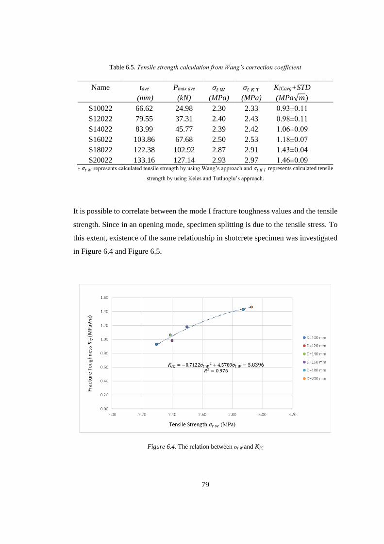
79
Table 6.5. Tensile strength calculation from Wang’s correction coefficient
Name
tave
(mm)
Pmax ave
(kN)
𝜎𝑡 𝑊
(MPa)
𝜎𝑡 𝐾 𝑇
(MPa)
KICavg+STD
(MPa√𝑚)
S10022 66.62 24.98 2.30 2.33 0.93±0.11
S12022 79.55 37.31 2.40 2.43 0.98±0.11
S14022 83.99 45.77 2.39 2.42 1.06±0.09
S16022 103.86 67.68 2.50 2.53 1.18±0.07
S18022 122.38 102.92 2.87 2.91 1.43±0.04
S20022 133.16 127.14 2.93 2.97 1.46±0.09 ∗ 𝜎𝑡 𝑊 represents calculated tensile strength by using Wang’s approach and 𝜎𝑡 𝐾 𝑇 represents calculated tensile
strength by using Keles and Tutluoglu’s approach.
It is possible to correlate between the mode I fracture toughness values and the tensile
strength. Since in an opening mode, specimen splitting is due to the tensile stress. To
this extent, existence of the same relationship in shotcrete specimen was investigated
in Figure 6.4 and Figure 6.5.
Figure 6.4. The relation between σt W and KIC
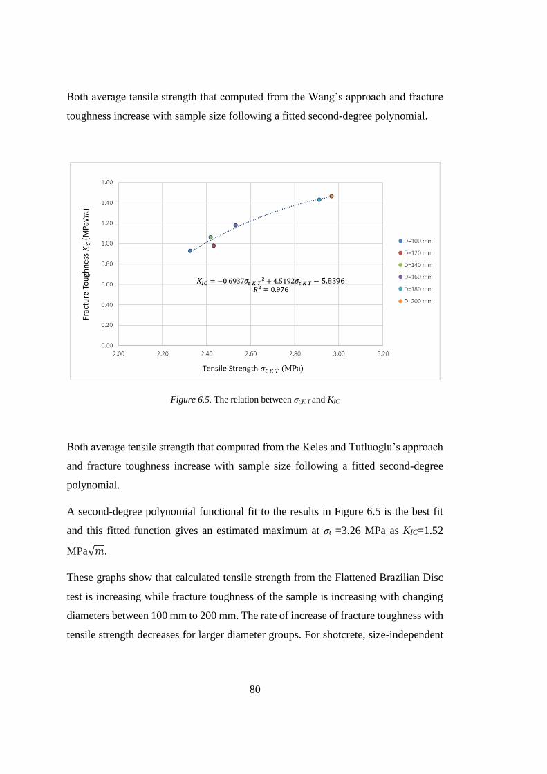
80
Both average tensile strength that computed from the Wang’s approach and fracture
toughness increase with sample size following a fitted second-degree polynomial.
Figure 6.5. The relation between σt,K T and KIC
Both average tensile strength that computed from the Keles and Tutluoglu’s approach
and fracture toughness increase with sample size following a fitted second-degree
polynomial.
A second-degree polynomial functional fit to the results in Figure 6.5 is the best fit
and this fitted function gives an estimated maximum at σt =3.26 MPa as KIC=1.52
MPa√𝑚.
These graphs show that calculated tensile strength from the Flattened Brazilian Disc
test is increasing while fracture toughness of the sample is increasing with changing
diameters between 100 mm to 200 mm. The rate of increase of fracture toughness with
tensile strength decreases for larger diameter groups. For shotcrete, size-independent

81
ratio between the fracture toughness and tensile strength is estimated as
KIC/σt=1.52/3.26=0.47 for the first time compared to the related literature.
Advancing this study, dimensionless fracture toughness over tensile strength ratio
changing with specimen size was investigated with tensile strength calculated using
Keles and Tutluoglu’s approach, which is a more recent study, in Figure 6.6.
Figure 6.6. Dimensionless toughness over tensile strength ratio
This polynomial function of degree three becomes zero at D=0.26 m meaning that size
independent fracture toughness and tensile strength is best measured for a diameter
range between 120-180 mm (best D=160 mm) tensile strength; after the tensile
strength increases too rapidly compared to fracture toughness taking curve down to
zero at 0.26 m diameter.


83
CHAPTER 7
7. CONCLUSION AND RECOMMENDATIONS
FBD geometry is used here for measuring the tensile strength and the tensile mode
fracture toughness of the molded shotcrete samples. For the FBD geometry,
compressive load at the flat ends results tension in the center, and crack is forced to
initiate at the center and propagate towards the loaded flattened ends. 3D printing
technology provides great advantages in terms of the accurate sample preparation
geometry for the desired diameter range of testing samples.
Size effect was clearly observed in results of seven day cured FBD testing work.
According to the American Shotcrete Association; concrete, when applied using the
shotcrete process, or cast-in-place, needs to cure for 7 days (American Shotcrete
Association, n.d.). Moreover, according to the American Concrete Institute (ACI)
often specified seven-day curing is recommend as a minimum curing period for Type
I cement in standards ASTM C 150. (Zemajtis, n.d.). Mode I fracture toughness values
at constant loading angle (22°) were increasing with the specimen diameter. The
average mode I fracture toughness, KIC avg for the largest diameter group (D=200 mm)
is about 1.57 times higher than the average mode I fracture toughness, KIC avg of the
smallest diameter group (D=100 mm). As the specimen gets larger, the crack tip gets
further from the compressively loaded area. In this case, the size of the fracture process
zone is relatively small compared to the specimen dimension, this can explain the
reason behind the higher fracture toughness values at higher diameters. Moreover,
another possible factor that lead to this increase can be explained as confining effect.
Shotcrete is a heterogeneous material; if a crack is forced to follow a strict path for a
large enough path in a large size disc, crack tip may be forced to break through both
binder and rather strong aggregate grains, resulting in a higher fracture toughness KIC.

84
According to the extreme points of the equation, it was predicted that after the
diameter increases up to around 205 mm, the increase in fracture toughness would not
continue.
In the size effect investigation, numerically computed and experimentally observed
crack lengths were compared. Shotcrete samples with rather large diameters showed
clearer local minimum load drops in the related load-displacement plots. Compared to
the numerically computed crack length/radius ratio acn/R of constant 0.72, ace/R ratio
increases with specimen diameter. The amount of increase is about 4%. This increase
is attributed to the size effect issue in the sense that inertia of unstably moving crack
is greater in a large size sample.
Considering the fact that shotcrete support unit provides temporary surface control of
underground openings, the effect of curing time on fracture toughness can be a
significant contribution. The early aged mixture design was used for the investigation
of curing time effect on the fracture toughness for specimens having diameter of 160
mm; KIC values increased about 79% with the curing time varying 1 day to 7 days.
In order to study the relation between fracture toughness and tensile strength, the
comparisons were made. After the results of several experimental works, it was
concluded that, up to a certain point tensile strength and the fracture toughness
increases proportionally.
The difference between the tensile strength obtained from the regular Brazilian Disc
test and the Flattened Brazilian Disc test can be explained by two reasons. The first
possible reason is the loading angle of the jaw used in the regular Brazilian Disc Test
is lower than the loading angle of the Flattened Brazilian Disc test. As the loading
angle decreases, fracture toughness is believed to increase, and thus tensile strength
increases too, since as found in this work, fracture toughness and tensile strength
increase proportionally. The second possible reason can be the loading differences.
While regular Brazilian Disc specimen is under an arc type loading because of the

85
steel jaws, the Flattened Brazilian Disc specimen is under the uniform diametrical
compression.
The Size effect phenomenon is effective on tensile strength obtained from the
Flattened Brazilian Disc test. With using two different approaches, Wang’s approach
and Keles & Tutluoglu’s approach, to obtain tensile strength from Flattened Brazilian
Disc tests results, tensile strength is found to increase with increasing diameter from
100 mm to 200 mm. There was a threshold diameter after which strength increased
with increasing disc size. Threshold diameter was around 200 mm.
In this study, for the shotcrete specimens that have 0.5 water/cement ratio, the size
effect on tensile strength was observed between 100 mm diameter and 200 mm. As a
result of fitted third degree polynomial function between the dimensionless fracture
toughness/tensile strength ratio and specimen diameter, the size-independent values
can be calculated in a diameter range between 120-180 mm (the best at 160 mm).
Tensile strength from FBD tests increased with increasing size. Explanation can be in
terms of crack tip stress field and a 3D yield criterion in terms of all principal stresses
(σ1, σ2, σ3). As diameter increases and specimen gets thicker, in-plane minimum
principal stresses and out of plane principal stresses change and perhaps increase in
compression. Use of a single yield criterion based on tensile strength and minimum
principal stress may not be the right approach to characterize the cracking failure for
this geometry. A yield criterion in terms of all principal stresses may be the choice for
describing the tensile cracking and surrounding stress distributions which are to be
inserted to 3-dimensional yield criteria.
For future work, it is suggested to use a stronger mold material to be used in the 3D
printer, since some molds broke before the tests are completed successfully. Another
recommendation is to extend this testing work for specimen sizes larger than the ones
used here. Also curing time work may involve more data points in the early ages of
curing, since this aging process is an important issue in carrying the expected loads in
a temporary support unit.

86
87
REFERENCES
Alexander M.G., Heiyantuduwa R. (2009). A Rewiew of Shotcrete Materials, Mix
Design and Applications. Shotcrete for Africa Conference.
Akbardoost, M. R. A. J. (2014). Size and Geometry Effects on Rock Fracture
Toughness: Mode I Fracture. Rock Mechanics and Rock Engineering, 677–687.
https://doi.org/10.1007/s00603-013-0430-7
American Shotcrete Association. (n.d.). Retrieved from
https://www.shotcrete.org/pages/products-services/technical-questions-
archive.htm
Anderson, T. L. (2005). Fracture mechanics: fundamentals and applications. CRC
Press.
Antolovich, S. D., Saxena, A., & Gerberich, W. W. (2018). Fracture mechanics – An
interpretive technical history. Mechanics Research Communications, 91, 46–86.
https://doi.org/10.1016/j.mechrescom.2018.03.003
Aydan, O., Sezaki, M. & Kawamoto, T. (1992), Mechanical and numerical modelling
of shotcrete, in Pande & Pietruszczak, eds, ‘Numerical Models in
Geomechanics’, pp. 757– 764.
Bazant, Z. P. (1976). Instability, Ductility and Size Effect in Strain-Softening
Concrete, Journal of the Engineering Mechanics Division, ASCE, Vol. 102, pp.
331-344.
Bazant, Z. P., & Kazemi, M. (1991). Size effect on diagonal shear failure of concrete
beams without stirrups. ACI Structural Journal 88(3), 268-276.

88
Bazant, Z. P., Kazemi,M.T, Hasegawa, T., Mazars, J. (1991). Size Effect in Brazilian
Split-Cylinder Tests: Measurements and Fracture Analysis. ACI Materials
Journal, 88.
Byfors, J. (1980), Plain concrete at early ages, Technical report, Swedish Cement and
Concrete Research Institute.
Carpinteri, A. (1984). Stability of Fracturing Process in RC Beams. Journal of
Structural Engineering, 110(3), 544–558. doi: 10.1061/(asce)0733-
9445(1984)110:3(544)
Ceriolo, L., & Di Tommaso, A. (1998). Fracture mechanics of brittle materials: An
historical point of view. Proceedings - 2nd International PhD Symposium in Civil
Engineering, (May), 207–214.
Chang, Y. (1994), Tunnel support with shotcrete in weak rock - A rock mechanics
study, PhD thesis, Royal Institute of Technology, Stockholm, Sweden.
Chong, K.P. and Kuruppu, M. D. (1984). New Specimen for Fracture Toughness
Determination
Cotterell, B. (2002). The past, present, and future of fracture mechanics. Engineering
Fracture Mechanics, 69(5), 533–553. https://doi.org/10.1016/S0013-
7944(01)00101-1
Dao, V., Dux, P., & Morris, P. H. (2014). Crack propagation in concrete at very early
ages. Magazine of Concrete Research, s. 643-651.
EN 206:2013+A1 Concrete - Specification, performance, production and conformity
standard.
Erdoğan, T.Y. (2013). Beton. Metu Press.

89
Fowell, R.J., “ISRM Commission on Testing Methods: Suggested Method for
Determining Mode I Fracture Toughness Using Cracked Chevron Notched
Brazilian Disc (CCNBD) Specimens”, Int. J. Rock Mech. Min. Sci. and
Geomech. Abstr.. Vol. 32, No. 1, pp. 57-64, 1995.
Griffith, A. A. (1921). The Phenomena of Rupture and Flow in Solids. Philosophical
Transactions of the Royal Society A: Mathematical, Physical and Engineering
Sciences, 221(582-593), 163–198. doi: 10.1098/rsta.1921.0006
Griffith, A.A. (1924). The Theory of Rupture, Proc. of First Int. Cong. Appl. Mech.,
pp. 53-64.
Gross, D. (2014). Some Remarks on the History of Fracture Mechanics. The History
of Theoretical, Material and Computational Mechanics - Mathematics Meets
Mechanics and Engineering Lecture Notes in Applied Mathematics and
Mechanics, 195–209. doi: 10.1007/978-3-642-39905-3_12
Guo, H., Aziz, N. I., & Schmidt, L. C. (1993). Rock fracture-toughness determination
by the Brazilian test. Engineering Geology, 33(3), 177–188.
https://doi.org/10.1016/0013-7952(93)90056-I
Hillerborg, A. (1985). The theoretical basis of a method to determine the fracture
energy G F of concrete. Materials and Structures, 18(4), 291–296.
https://doi.org/10.1007/BF02472919
Hillerborg, A., Modeer, M., & Petersson, P. (1976). Analysis of crack formation and
growth in concrete be means of fracture mechanics and finite elements. Cement
& Concrete Research Vol.6, 773-782.
Irwin, G. (1958). Fracture. Handbuch der Physik (s. 551-590). içinde Berlin: Springer.
90
ISRM. (1979). Suggested Methods for Determining the Uniaxial Compressive
Strength. Int. J. Rock Mech. Min. Sci. & Geomech, 135-140.
Japaridze, L. (2015). Stress-deformed state of cylindrical specimens during indirect
tensile strength testing. Journal of Rock Mechanics and Geotechnical
Engineering, 7(5), 509–518. doi: 10.1016/j.jrmge.2015.06.006
Jenq, Y., & Shah, S. P. (1985). Two Parameter Fracture Model for Concrete. Journal
of Engineering Mechanics, 111(10), 1227–1241. doi: 10.1061/(asce)0733-
9399(1985)111:10(1227)
Kaklis, K. N., Agioutantis, Z., Sarris, E., & Pateli, A. (2005). A theoretical and
numerical study of discs with flat edges under diametral compression (flat
Brazilian test). 5th GRACM International Congress on Computational
Mechanics, 29(June 2017).
Kaplan, M. (1961). Crack propagation and the fracture of concrete. Journal of ACI
Vol.58, 591-610.
Karihaloo, B., & Nallathambi, P. (1989). An improved effective crack model for the
determination of fracture toughness of concrete. Cement and Concrete Research,
19(4), 603–610. doi: 10.1016/0008-8846(89)90012-4
Keles, C., & Tutluoglu, L. (2011). Investigation of proper specimen geometry for
mode I fracture toughness testing with flattened Brazilian disc method. Int. J.
Frac. , 61-75.
Kesler, C., Naus, D., & Lott, J. (1971). Fracture mechanics its applicability to
concrete. The Society of Material Science Vol.4, 113-124.
Key to Metals Database, http://steel.keytometals.com, last visited on 24th March
2010.
91
Kuruppu, M. D., Obara, Y., Ayatollahi, M.R., Chong, K.P., & Funatsu, T. (2015)
ISRM- suggested method for determining the mode I static fracture toughness
using semi- circular bend specimen. In the ISRM Suggested Methods for Rock
Characterization, Testing and Monitoring: 2007-2014, 107-114. Springer
International Publishing
Liang, P., & Tao, J. (2014). The Contrast of Concrete Brazilian and Flattened
Brazilian Disc. Applied Mechanics and Materials , s. 263-268.
Mahanta, B., Sirdesai, N., Singh, T. N., & Ranjith, P. G. (2017). Experimental Study
of Strain Rate Sensitivity to Fracture Toughness of Rock using Flattened
Brazilian Disc. In Procedia Engineering (Vol. 191, pp. 256–262). The Author(s).
https://doi.org/10.1016/j.proeng.2017.05.179
McClintock, F.A. and J.B. Walsh (1962). Friction of Griffith cracks in rock under
pressure. Proc. Fourth U.S. Congr. Appl. Mech. 1015-21. Berkeley: American
Society of Mechanical Engineers.
Miner, G. M. (1973). Use of shotcrete from the standpoint of the owner. Use of
Shotcrete for Underground Structural Support. South Berwick: American
Society of Civil Engineers and American Concrete Institute.
Nallathambi, P., & Karihaloo, B. (1986). Determination of the specimen size
independent fracture toughness of plain concrete. Magazine of Concrete
Research Vol. 38, 67-76.
Neville, A. (1981), Properties of concrete, Longman Scientific & Technical.
Ouchterlony, F., “ISRM Commission on Testing methods; Suggested Methods for
determining fracture toughness of rock”, Int. J. Rock Mech. Min. Sci. &
Geomech. Abstr., Vol. 25, pp. 71-96, 1988.

92
Özdoğan, C. (2017). Pure tensile fracture modelling and toughness measurements on
brazilian discs of andesite and marble. Ankara.
Perdikaris, P. C., Calomino, A. M., & Chudnovsky, A. (1986, August). Effect of
Fatigue on Fracture Toughness of Concrete. Journal of Engineering Mechanics,
s. 776-791.
Rossmanith, H. (1983). Rock Fracture Mechanics (Cilt 68). (I. C. Sciences, Dü.)
Wien-New York: Springer-Verlag.
Shah, S. P. (1995). Fracture Mechanics of Concrete, Applications of Fracture
Mechanics to Concrete, Rock and Other Quasi-Brittle Materials. NY: A Wiley-
Interscience Publication.
Sheity, D. K., Rosenfield, A. R., & Duckworth, W. H. (1985). Fracture Toughness of
Ceramics Measured by a Chevron-Notch Diametral-Compression Test. Journal
of the American Ceramic Society, 68(12). doi:10.1111/j.1151-
2916.1985.tb10135.x
SIKA. (2001). SIKA ViscoCrete Hi-Tech.
Timoshenko, S.P. and Goodier, J.N. (1970). Theory of Elasticity. 3rd Edition, Mc
Graw-Hill, New York.
Ulusay, R., & Hudson, J. A. (2007). The Complete ISRM Suggested Methods for Rock
Characterization, Testing and Monitoring: 1974-2006. Ankara.
Walsh, P. F. (1979). Fracture of Plain Concrete, The Indian Concrete Journal, Vol.
46, No. 11, pp. 469-470, and 476.
Wang, Q.Z., Jia, X.M., Kou, S.Q., Zhang, Z.X. and Lindqvist, P.A. (2004). The
Flattened Brazilian Disc Specimen Used for Testing Elastic Modulus, Tensile

93
Strength and Fracture Toughness of Brittle Rocks: Analytical and Numerical
Results. Int. J. of Rock Mech. Min. Sci., Vol. 41, pp. 245-253.
Wang, Q. Z., & Wu, L. Z. (2004). The flattened Brazilian disc specimen used for
determining elastic modulus, tensile strength and fracture toughness of brittle
rocks: Experimental results. International Journal of Rock Mechanics and
Mining Sciences, 41(SUPPL. 1), 1–5.
https://doi.org/10.1016/j.ijrmms.2004.03.015
Wang, Q. Z., & Xing, L. (1999). Determination of fracture toughness KIc by ussing
the flattened Brazilian dics specimen for rocks. Engineering Fracture Mechanics
(64), 193-201.
Zemajtis, J. Z. (n.d.). PCA: Portland Cement Association. Role of Concrete Curing:
Retrieved from https://www.cement.org/learn/concrete-technology/concrete-
construction/curing-in-construction
Zhao, X. L., Fowell, R. J., Roegiers, J. C., & Xu, C. (1994). Rock fracture-toughness
determination by the Brazilian test, by H. Guo, N.I. Aziz, L.C. Schmidt.
Engineering Geology, 38(1–2), 181–184. https://doi.org/10.1016/0013-
7952(94)90033-7

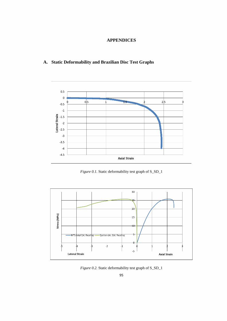
95
APPENDICES
A. Static Deformability and Brazilian Disc Test Graphs
Figure 0.1. Static deformability test graph of S_SD_1
Figure 0.2. Static deformability test graph of S_SD_1
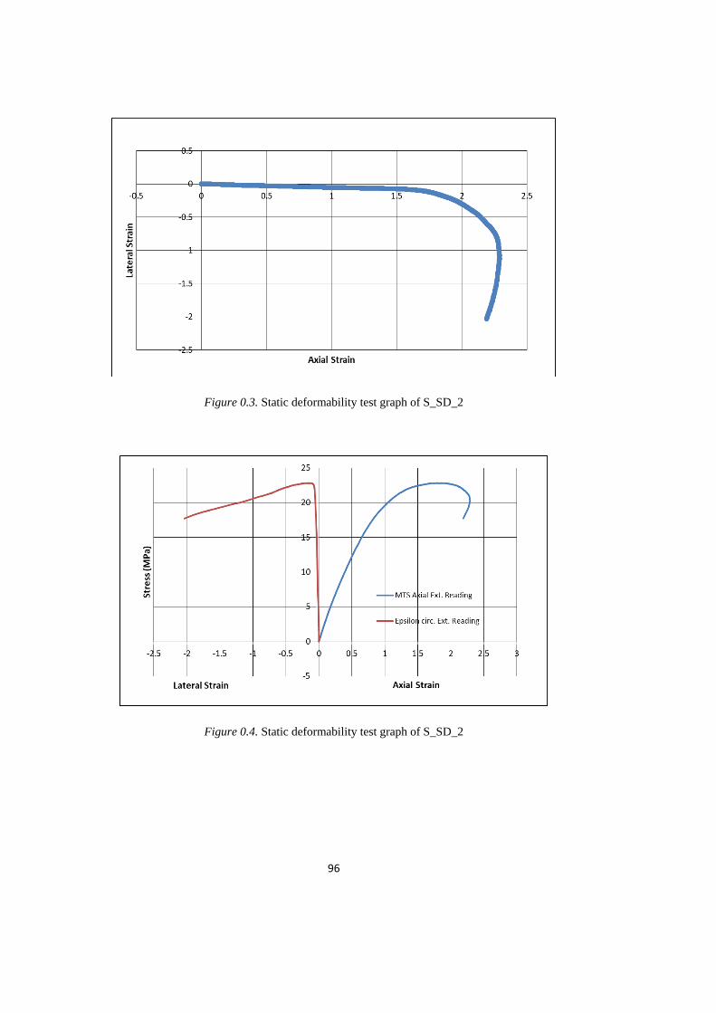
96
Figure 0.3. Static deformability test graph of S_SD_2
Figure 0.4. Static deformability test graph of S_SD_2

97
Figure 0.5. Static deformability test graph of S_SD_3
Figure 0.6. Static deformability test graph of S_SD_3
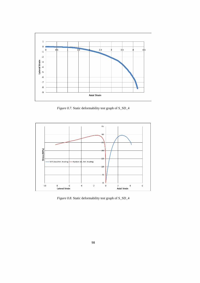
98
Figure 0.7. Static deformability test graph of S_SD_4
Figure 0.8. Static deformability test graph of S_SD_4

99
Figure 0.9. Static deformability test graph of S_SD_5
Figure 0.10. Static deformability test graph of S_SD_5

100
Figure 0.11. Brazilian Disc test graph of S_BD_1
Figure 0.12. Brazilian Disc test graph of S_BD_2

101
Figure 0.13. Brazilian Disc test graph of S_BD_3
Figure 0.14. Brazilian Disc test graph of S_BD_4
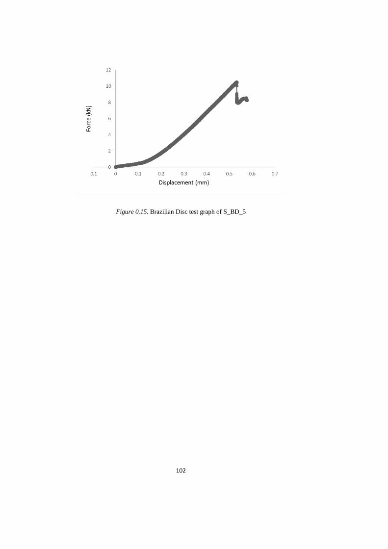
102
Figure 0.15. Brazilian Disc test graph of S_BD_5
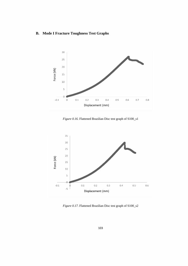
103
B. Mode I Fracture Toughness Test Graphs
Figure 0.16. Flattened Brazilian Disc test graph of S100_s1
Figure 0.17. Flattened Brazilian Disc test graph of S100_s2

104
Figure 0.18. Flattened Brazilian Disc test graph of S100_s3
Figure 0.19. Flattened Brazilian Disc test graph of S100_s4

105
Figure 0.20. Flattened Brazilian Disc test graph of S100_s5
Figure 0.21. Flattened Brazilian Disc test graph of S120_s1
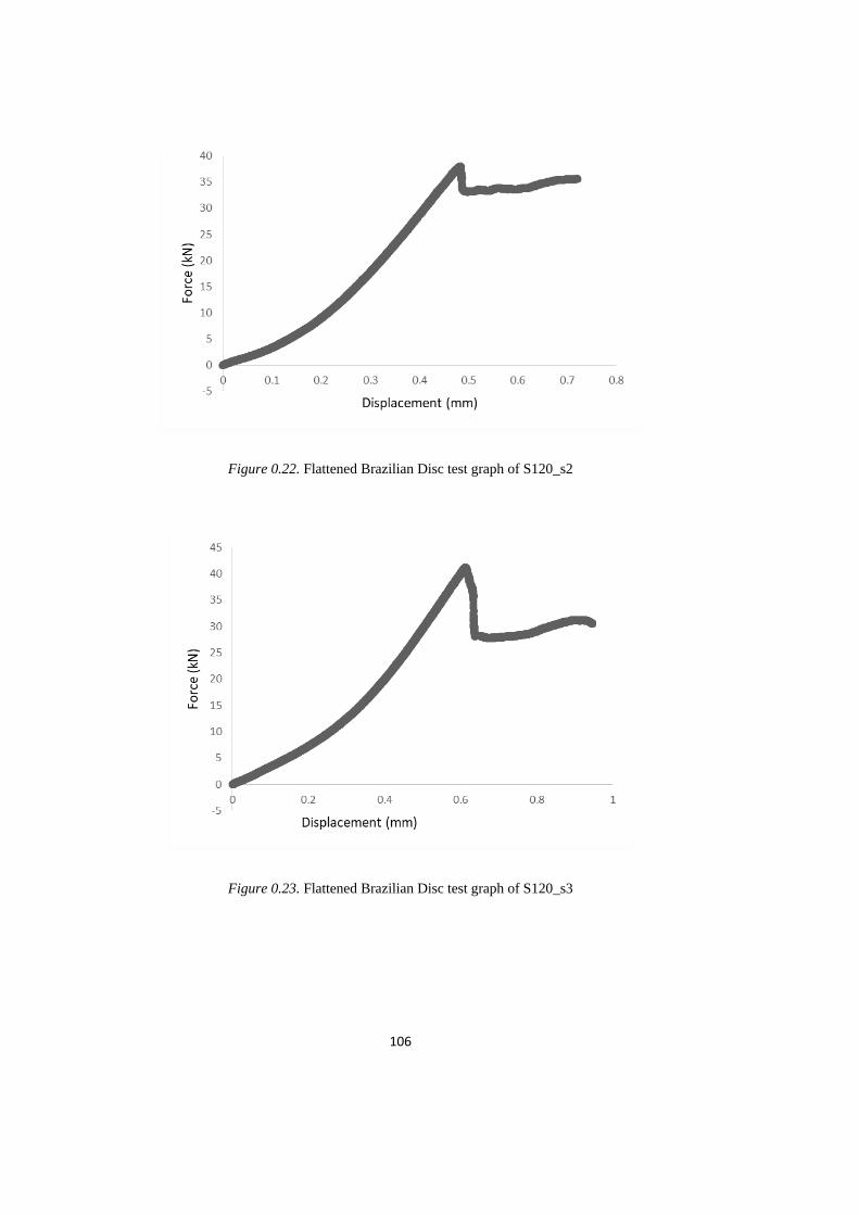
106
Figure 0.22. Flattened Brazilian Disc test graph of S120_s2
Figure 0.23. Flattened Brazilian Disc test graph of S120_s3
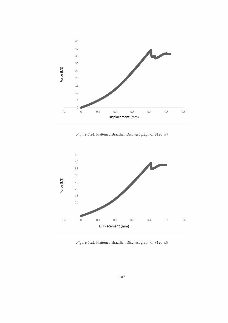
107
Figure 0.24. Flattened Brazilian Disc test graph of S120_s4
Figure 0.25. Flattened Brazilian Disc test graph of S120_s5
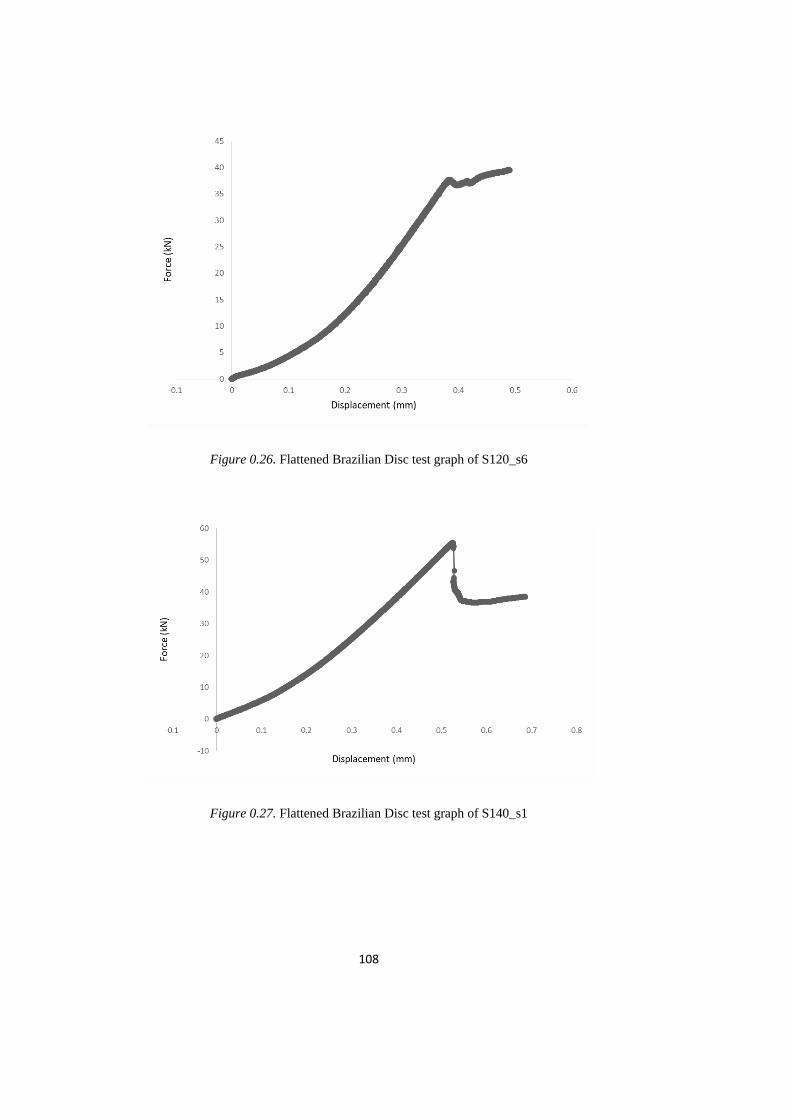
108
Figure 0.26. Flattened Brazilian Disc test graph of S120_s6
Figure 0.27. Flattened Brazilian Disc test graph of S140_s1
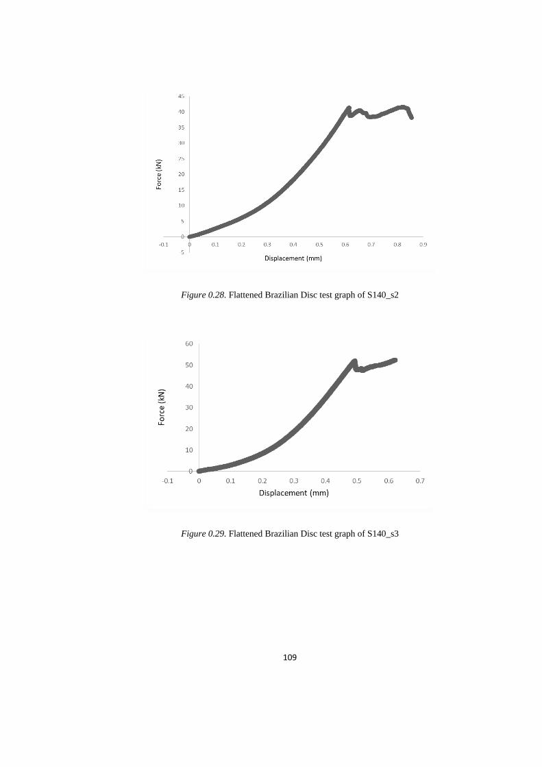
109
Figure 0.28. Flattened Brazilian Disc test graph of S140_s2
Figure 0.29. Flattened Brazilian Disc test graph of S140_s3

110
Figure 0.30. Flattened Brazilian Disc test graph of S140_s4
Figure 0.31. Flattened Brazilian Disc test graph of S140_s5
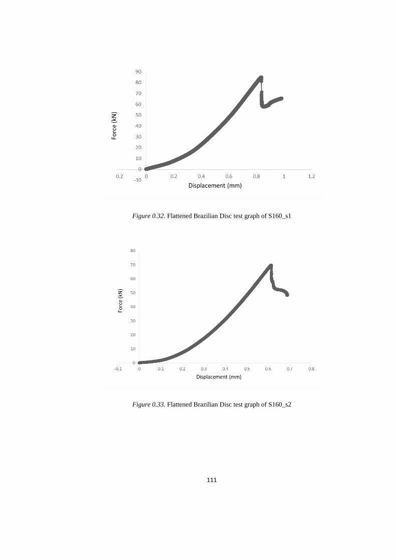
111
Figure 0.32. Flattened Brazilian Disc test graph of S160_s1
Figure 0.33. Flattened Brazilian Disc test graph of S160_s2

112
Figure 0.34. Flattened Brazilian Disc test graph of S160_s3
Figure 0.35. Flattened Brazilian Disc test graph of S160_s4
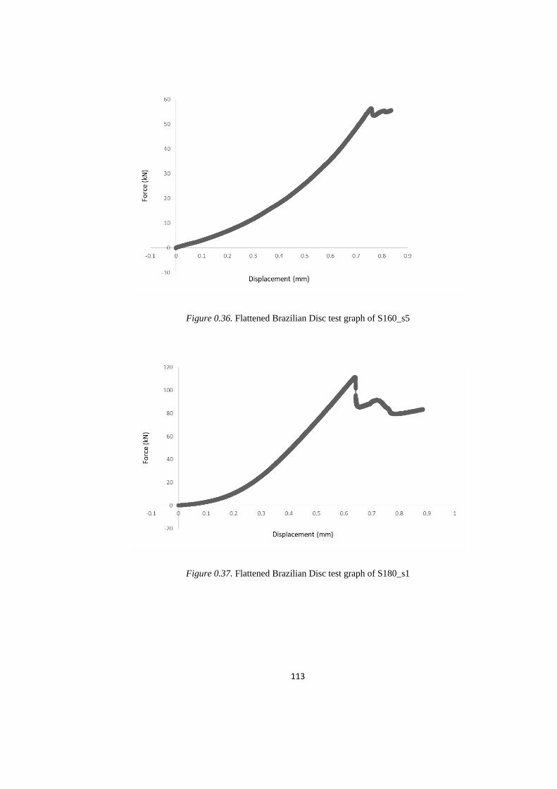
113
Figure 0.36. Flattened Brazilian Disc test graph of S160_s5
Figure 0.37. Flattened Brazilian Disc test graph of S180_s1
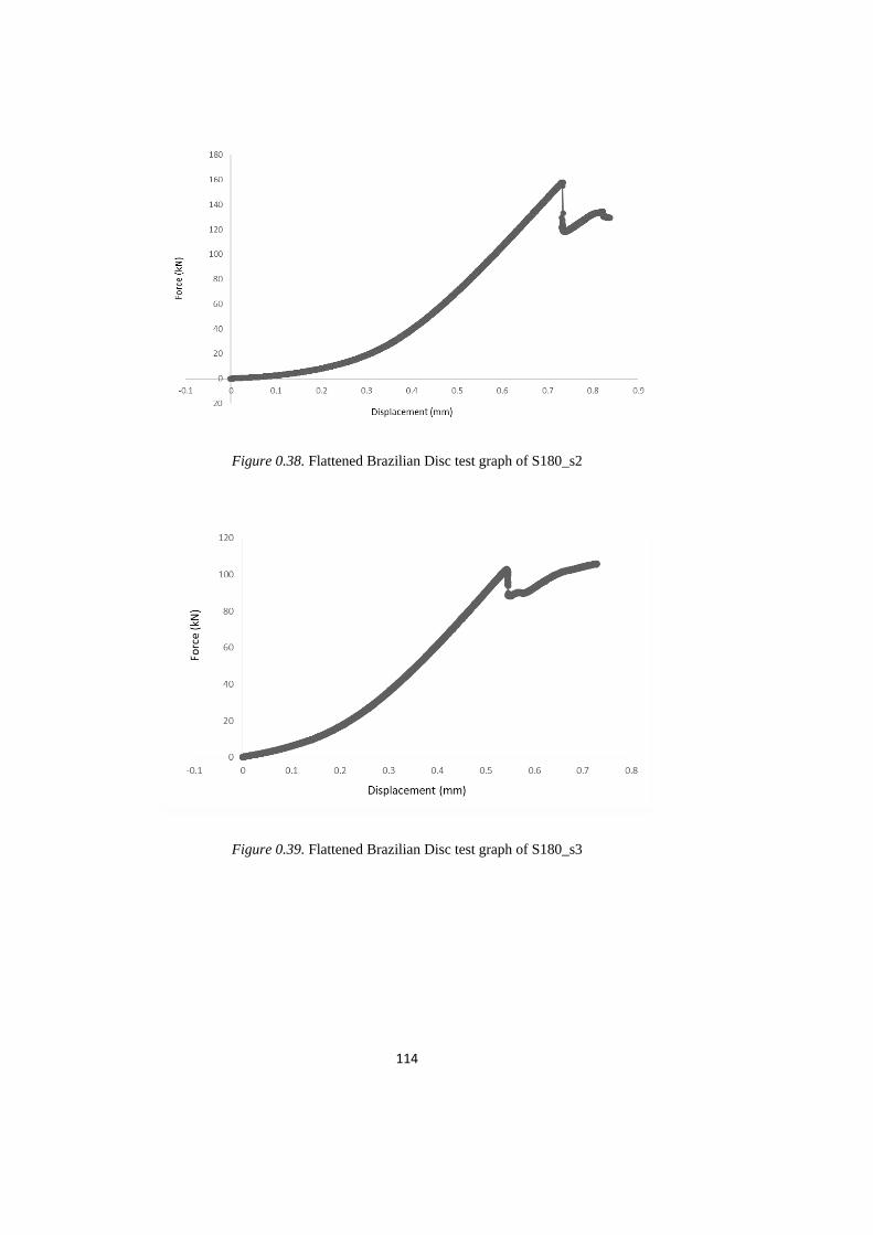
114
Figure 0.38. Flattened Brazilian Disc test graph of S180_s2
Figure 0.39. Flattened Brazilian Disc test graph of S180_s3

115
Figure 0.40. Flattened Brazilian Disc test graph of S180_s4
Figure 0.41. Flattened Brazilian Disc test graph of S180_s5

116
Figure 0.42. Flattened Brazilian Disc test graph of S200_s1
Figure 0.43. Flattened Brazilian Disc test graph of S200_s2

117
Figure 0.44. Flattened Brazilian Disc test graph of S200_s3
Figure 0.45. Flattened Brazilian Disc test graph of S200_s4

118
Figure 0.46. Flattened Brazilian Disc test graph of S160-1D-s1
Figure 0.47. Flattened Brazilian Disc test graph of S160-1D-s2
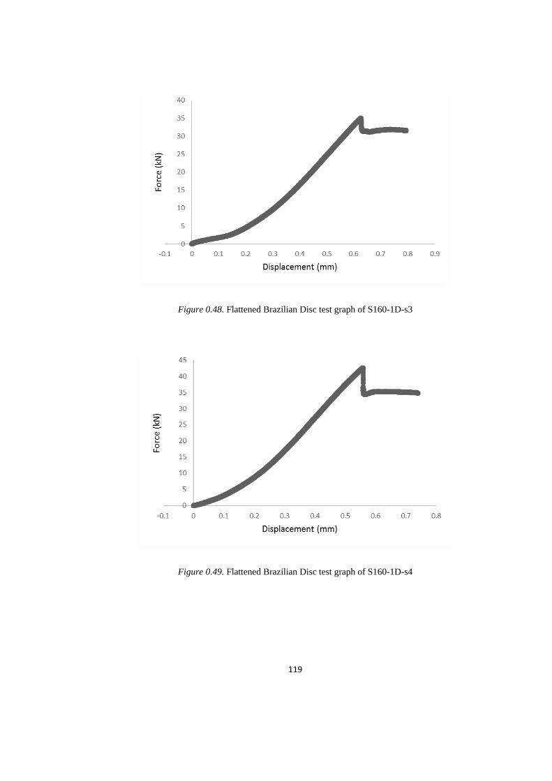
119
Figure 0.48. Flattened Brazilian Disc test graph of S160-1D-s3
Figure 0.49. Flattened Brazilian Disc test graph of S160-1D-s4

120
Figure 0.50. Flattened Brazilian Disc test graph of S160-2D-s1
Figure 0.51. Flattened Brazilian Disc test graph of S160-2D-s2

121
Figure 0.52. Flattened Brazilian Disc test graph of S160-2D-s3
Figure 0.53. Flattened Brazilian Disc test graph of S160-2D-s4
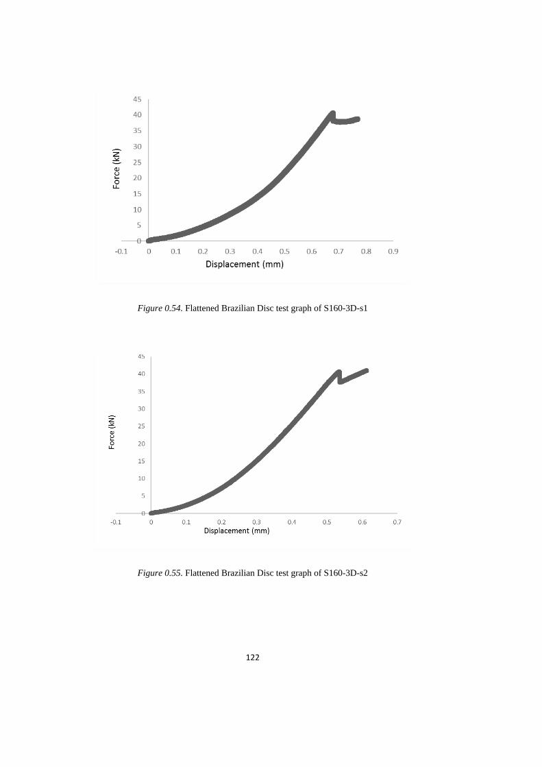
122
Figure 0.54. Flattened Brazilian Disc test graph of S160-3D-s1
Figure 0.55. Flattened Brazilian Disc test graph of S160-3D-s2
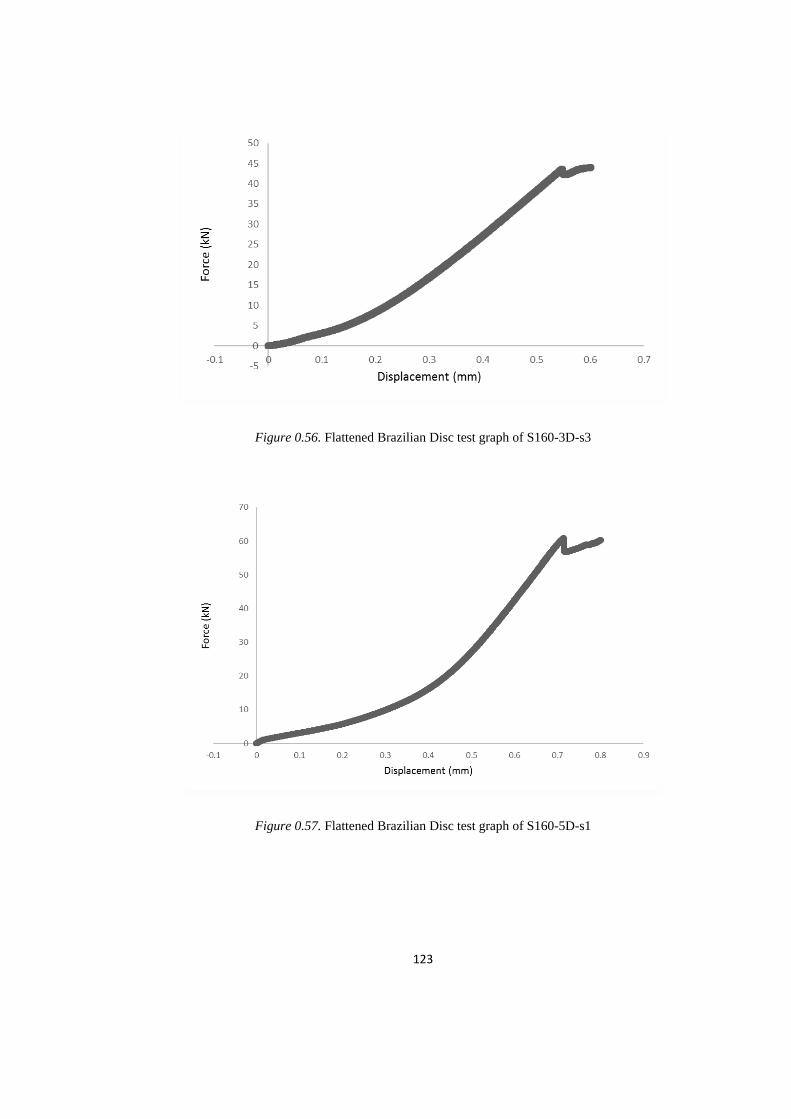
123
Figure 0.56. Flattened Brazilian Disc test graph of S160-3D-s3
Figure 0.57. Flattened Brazilian Disc test graph of S160-5D-s1
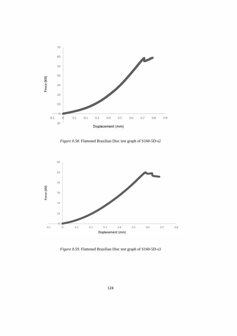
124
Figure 0.58. Flattened Brazilian Disc test graph of S160-5D-s2
Figure 0.59. Flattened Brazilian Disc test graph of S160-5D-s3

125
Figure 0.60. Flattened Brazilian Disc test graph of S160-5D-s4


127
C. Crack Length Measurement of Mode I Fracture Toughness Test Samples
Figure 0.61. FBD test crack measurement of the sample S100_s1
Figure 0.62. FBD test crack measurement of the sample S100_s2
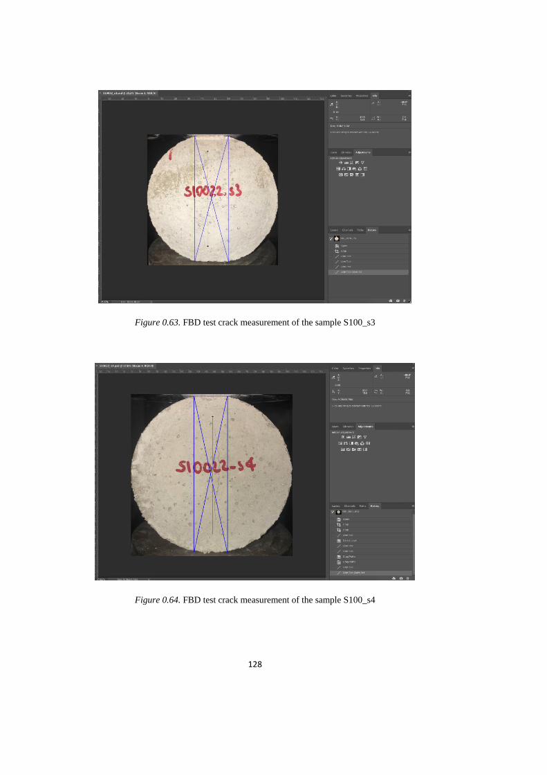
128
Figure 0.63. FBD test crack measurement of the sample S100_s3
Figure 0.64. FBD test crack measurement of the sample S100_s4

129
Figure 0.65. FBD test crack measurement of the sample S100_s5
Figure 0.66. FBD test crack measurement of the sample S120_s1

130
Figure 0.67. FBD test crack measurement of the sample S120_s2
Figure 0.68. FBD test crack measurement of the sample S120_s3
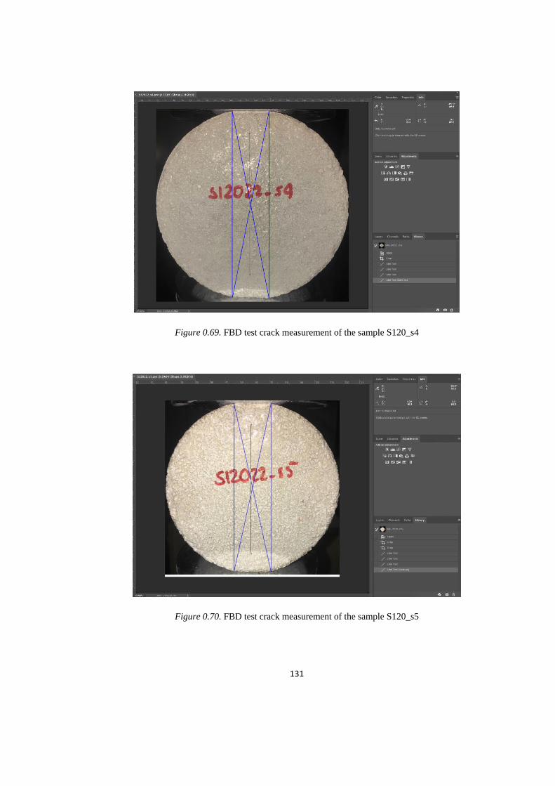
131
Figure 0.69. FBD test crack measurement of the sample S120_s4
Figure 0.70. FBD test crack measurement of the sample S120_s5
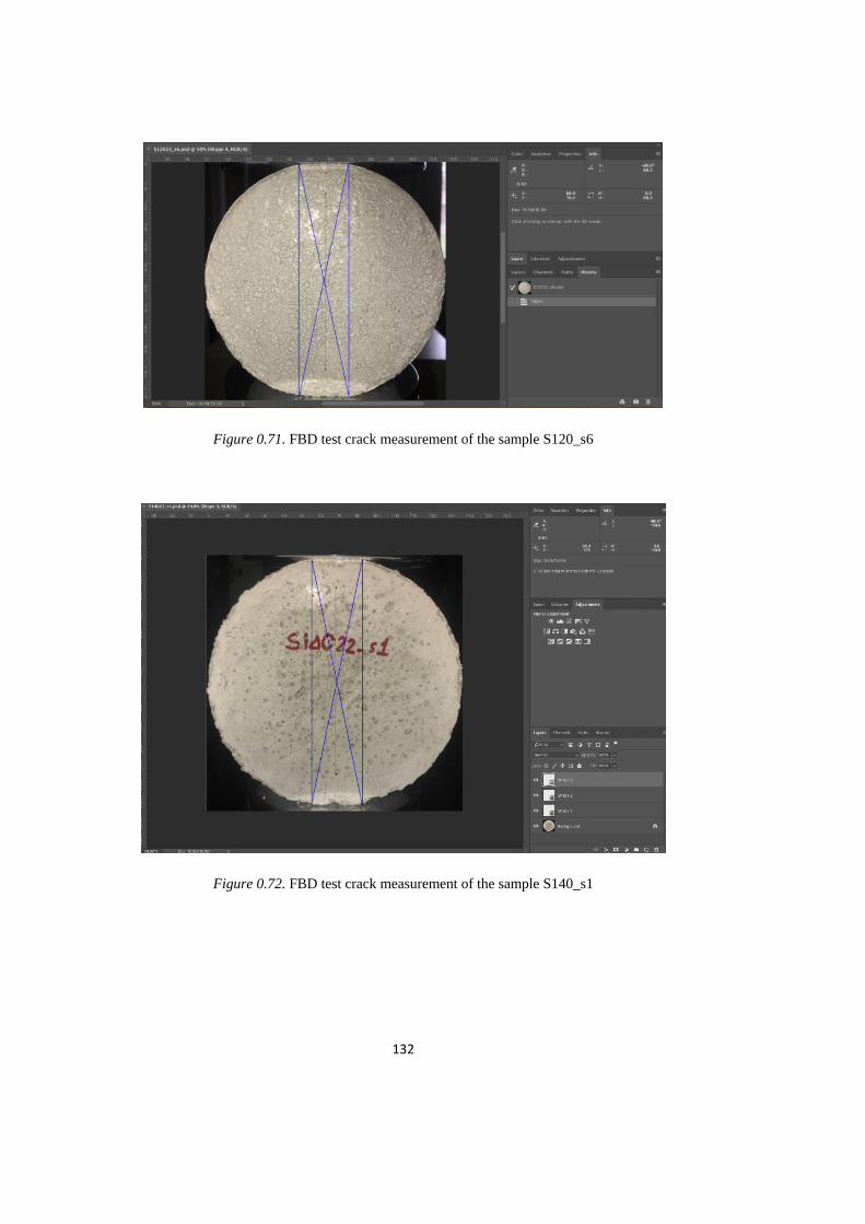
132
Figure 0.71. FBD test crack measurement of the sample S120_s6
Figure 0.72. FBD test crack measurement of the sample S140_s1

133
Figure 0.73. FBD test crack measurement of the sample S140_s2
Figure 0.74. FBD test crack measurement of the sample S140_s3
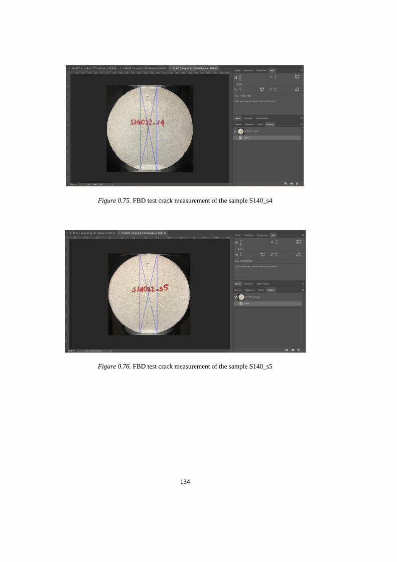
134
Figure 0.75. FBD test crack measurement of the sample S140_s4
Figure 0.76. FBD test crack measurement of the sample S140_s5

135
Figure 0.77. FBD test crack measurement of the sample S160_s1
Figure 0.78. FBD test crack measurement of the sample S160_s2

136
Figure 0.79. FBD test crack measurement of the sample S160_s3
Figure 0.80. FBD test crack measurement of the sample S160_s4
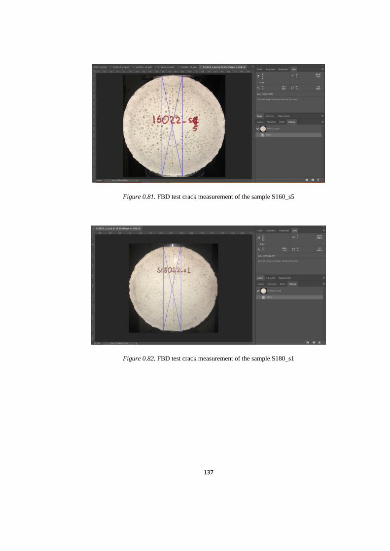
137
Figure 0.81. FBD test crack measurement of the sample S160_s5
Figure 0.82. FBD test crack measurement of the sample S180_s1
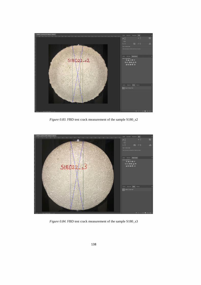
138
Figure 0.83. FBD test crack measurement of the sample S180_s2
Figure 0.84. FBD test crack measurement of the sample S180_s3

139
Figure 0.85. FBD test crack measurement of the sample S180_s4
Figure 0.86. FBD test crack measurement of the sample S180_s5

140
Figure 0.87. FBD test crack measurement of the sample S200_s1
Figure 0.88. FBD test crack measurement of the sample S200_s2
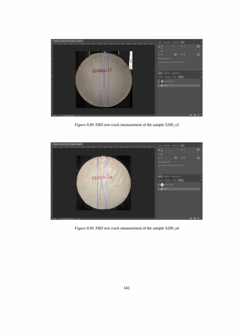
141
Figure 0.89. FBD test crack measurement of the sample S200_s3
Figure 0.90. FBD test crack measurement of the sample S200_s4
