modal basis approaches in shape and topology optimization

HAL Id: hal-01354162https://hal.archives-ouvertes.fr/hal-01354162

Submitted on 17 Aug 2016

HAL is a multi-disciplinary open accessarchive for the deposit and dissemination of sci-entific research documents, whether they are pub-lished or not. The documents may come fromteaching and research institutions in France orabroad, or from public or private research centers.

L’archive ouverte pluridisciplinaire HAL, estdestinée au dépôt et à la diffusion de documentsscientifiques de niveau recherche, publiés ou non,émanant des établissements d’enseignement et derecherche français ou étrangers, des laboratoirespublics ou privés.

Modal basis approaches in shape and topologyoptimization of frequency response problems

Grégoire Allaire, Georgios Michailidis

To cite this version:Grégoire Allaire, Georgios Michailidis. Modal basis approaches in shape and topology optimizationof frequency response problems. International Journal for Numerical Methods in Engineering, Wiley,2018, 113 (8), pp.1258-1299. hal-01354162

https://hal.archives-ouvertes.fr/hal-01354162

https://hal.archives-ouvertes.fr

Modal basis approaches in shape and topology optimization

of frequency response problems

Gregoire AllaireCMAP, Ecole Polytechnique, CNRS, Universite Paris-Saclay,

91128 Palaiseau, France([email protected])

Georgios MichailidisSIMaP-Universite de Grenoble, INPG,

38000 Grenoble, France([email protected])

July 14, 2016

Abstract

The optimal design of mechanical structures subject to periodic excitations within a largefrequency interval is quite challenging. In order to avoid bad performances for non-discretizedfrequencies, it is necessary to finely discretize the frequency interval, leading to a very largenumber of state equations. Then, if a standard adjoint-based approach is used for optimization,the computational cost (both in terms of CPU and memory storage) may be prohibitive forlarge problems, especially in three space dimensions. The goal of the present work is tointroduce two new non-adjoint approaches for dealing with frequency response problems inshape and topology optimization. In both cases, we rely on a classical modal basis approachto compute the states, solutions of the direct problems. In the first method, we do not useany adjoint but rather directly compute the shape derivatives of the eigenmodes in the modalbasis. In the second method, we compute the adjoints of the standard approach by usingagain the modal basis. The numerical cost of these two new strategies are much smaller thanthe usual ones if the number of modes in the modal basis is much smaller than the number ofdiscretized excitation frequencies. We present numerical examples for the minimization of thedynamic compliance in two and three space dimensions.

Keywords: shape and topology optimization, frequency response, level-set method

1 Introduction

Shape and topology optimization techniques [1, 5, 9] find today extensive applications in industryrelated to product design. Its incorporation in the design cycle can significantly reduce the requiredtime for the conception of a mechanical part and improve its performance. Especially when themechanical framework of the application is complicated enough, relying only on the experienceand intuition of engineers frequently proves to be not efficient enough. In such cases, performance-driven automated design techniques can provide a powerful remedy, allowing designers to enrichtheir knowledge and result in better designs.

Frequency response problems appear in a wide variety of industries, such as the automotive andthe aeronautic sectors. Such problems are characterized by a Helmholtz state equation, featuring

1

the excitation frequency and possibly some damping, and furthermore by the fact that usuallyone is not interested by a single frequency but rather by a whole interval of excitation frequencies.Discretization of the frequency range yields a large number of Helmholtz state equations. Contraryto multiple loads optimization where the state equation is the same and only the right handsides vary, frequency response optimization leads to a collection of different partial differentialequations or rigidity matrices. As a consequence, the computational cost of frequency responseoptimization is very large and even prohibitive for industrial applications with large-scale problems.This is all the more an issue since the frequency interval must be finely discretized otherwiseintermediate frequencies in a gap between two discretized frequencies may lead to completelysuboptimal performances.

In order to reduce the computational cost of frequency response optimization, a classical ap-proach is to work with a modal basis. In other words, for a given structure, one computes itsfirst eigenfrequencies and eigenmodes (without damping) in a range covering the entire excitationfrequency interval. Then, the Helmholtz state equations (with damping) are solved by a Galerkinmethod with this modal basis. In the context of shape and topology optimization, this additionallyrequires the solution of an adjoint problem for every eigenfrequency. Since the number of eigen-frequencies of the modal basis can be quite large, the total cost of this approach can be indeedprohibitive for industrial applications.

There is already a vast literature for topology optimization of frequency response problemsand we give a brief and non exhaustive account of it. Early works were done in the framework ofthe homogenization method: Ma et al. [19], [20] minimized the mean compliance in a frequencyinterval using a direct and a modal analysis, while Min et al. [21] used an optimality criteriamethod to minimize the dynamic compliance, working in the time domain. In the context of platethickness optimization, Jog [16] worked on the dynamic compliance and the frequency amplitude.Later, many more works appeared using the SIMP method. Tcherniak [32] presented a method,based on modal analysis, for the design of resonating structures. Olhoff et al. [23] and Yoon [34]studied the dynamic compliance minimization. A very interesting paper was written by Jensen[15] in order to accelerate the sensitivity computations: he proposed to use Pade approximantsfor the solution of dynamic problems, avoiding the costly calculation of adjoint states for manyexcitation frequencies. Finally, in the level-set framework (that we adopt in the present article)the first work about frequency response problems is that of Shu et al. [29].

Here, our main goal is to present two new methods for the treatment of frequency responseproblems, which do not require the computation of adjoint states, and thus accelerate significantlythe optimization process and make feasible the application of shape and topology optimizationon industrial frequency response problems. Although the proposed methods can be applied in theframework of density-based methods too, we use here the level-set method for the shape description[2, 3, 25, 28, 33], in order to benefit both from its geometric advantage of a clear definition of ashape and to avoid possible ghost modes in the modal analysis, localized in region of intermediatedensities.

The content of the present paper is as follows. Section 2 is devoted to a general presentationof the mechanical framework and of the optimization setting for frequency response problems.Section 3 is a brief introduction to the basic ingredients for shape and topology optimization viathe level-set method. For reasons of completeness, the standard adjoint approach is recalled inSection 4. The main conclusion is that it leads to as many adjoint states as there are discreteexcitation frequencies, which is totally prohibitive from a numerical point of view. Section 5describes what is more or less the state of the art in frequency response problems. A modal basisapproach is used to compute the solutions of the Helmholtz state equations. By considering thespectral equations as the effective state equations, the optimization process leads to consider newadjoint equations, the number of which is roughly the number of eigenfrequencies in the modalbasis. Although it is a serious improvement with respect to the previous standard approach of

2

Section 4, it is still a very costly strategy in terms of computation time and memory storage. Ourfirst new self-adjoint method is presented in Section 6: it is based on the approximation of theeigenmodes’ shape derivatives in the modal basis and requires no adjoint equations. Note thatthis method, as well as the next one, can cope with damping as long as the damping operator isdiagonal in the modal basis, as is often the case in numerical practice. A second new self-adjointmethod is proposed in Section 7. Its principle is quite simple: it starts from the standard shapederivative obtained in Section 4 and replace the direct and adjoint states by their approximationin the modal basis, therefore eliminating the need of solving any adjoint equations. A comparisonof all these approaches is performed in Section 8 in terms of complexity or operation counts. Itshows that our two proposed self-adjoint methods outperform the other approaches as soon as thenumber of discretized excitation frequencies and the number of eigenfrequencies in the modal basisare large. Of course, a key issue for numerical efficiency is to have access to a fast and accuratealgorithm to compute the modal basis. Section 9 is an assessment of the modal basis approach.We discuss convergence issues in terms of the number of eigenmodes and of the discretization stepfor the excitation frequency interval. Finally, numerical results in two and three space dimensionsare shown in Section 10, which validates our proposed approach. We focus on dynamic complianceminimization problems but other objective functions would work as well in our setting. We alsocheck that multiple eigenvalues are not an issue from a numerical point of view, although it isknown to be a delicate point when it comes to their differentiability properties.

2 Setting of the problem

2.1 State equation

Consider a structure, occupying a bounded domain Ω ⊂ Rd, with d = 2, 3, which vibrates underthe application of a periodic time-harmonic load f(x, t) at some part of its boundary ΓN ⊂ ∂Ω.The structure is fixed at ΓD ⊂ ∂Ω, while the rest of its boundary, denoted Γ, is free and subjectto optimization. The corresponding displacement field u(x, t) is a solution of the system

ρ(x)u+ c(x)u− div (Ae(u)) = 0 in Ω× R+,u = 0 on ΓD × R+,(

Ae(u))n = f(t) on ΓN × R+,(

Ae(u))n = 0 on Γ× R+,

(1)

where ρ(x) > 0 is the material density, c(x) ≥ 0 the damping function, A the isotropic Hooke’s law,e(u) = (∇u+ (∇u)T )/2 the strain tensor and the dot ( ˙ ) denotes derivation with respect to time.Since we are looking for a time-harmonic displacement u(x, t), we did not include initial conditionsin (1). To facilitate the analysis, we work with complex-valued functions (with i =

√−1). Assume

the complex loading to be of the type

f(x, t) = F (x)eiωt, F = fRe + ifIm, fRe, fIm ∈ R, (2)

where ω > 0 is the excitation frequency and F the complex loading amplitude. Similarly we lookfor a complex time-harmonic solution of (1) which reads as

u(x, t) = U(x)eiωt, U = uRe + iuIm, uRe, uIm ∈ R. (3)

3

One recovers a real-valued solution of (1) by taking the real part Re(u) = uRe cos(ωt)−uIm sin(ωt).Substituting (3) in (1), we obtain the equation satisfied by the displacement amplitude U :

−ω2ρU + iωcU − div (Ae(U)) = 0 in Ω,U = 0 on ΓD,(

Ae(U))n = F on ΓN ,(

Ae(U))n = 0 on Γ.

(4)

In the sequel we shall always work in the frequency domain, rather than in the time domain.Namely, we use (4) as the state equation, instead of (1). Separating the real and imaginary parts,we get the following two coupled systems of PDE’s:

−ω2ρuRe − ωcuIm − div (Ae(uRe)) = 0 in Ω,uRe = 0 on ΓD,(

Ae(uRe))n = fRe on ΓN ,(

Ae(uRe))n = 0 on Γ,

(5)

and −ω2ρuIm + ωcuRe − div (Ae(uIm)) = 0 in Ω,

uIm = 0 on ΓD,(Ae(uIm)

)n = fIm on ΓN ,(

Ae(uIm))n = 0 on Γ.

(6)

Remark 2.1. For given loads fRe, fIm ∈ L2(ΓN )d and in the presence of damping, i.e. c(x) ≥ 0and c 6= 0, the system of equations (5), (6) has a unique solution uRe, uIm ∈ H1(Ω)d (see e.g.Lemma 2.6.6 in [22]). In the undamped case (c = 0), a unique solution exists when the frequencyof the external loading does not coincide with an eigenfrequency of the structure. Note that in thesequel, we shall often replace the damping multiplicative coefficient c(x) by a diagonal operator Cin the modal basis (see Section 5 for more details).

Remark 2.2. For simplicity, and because it is enough in many applications, we consider onlysurface loads on ΓN . However, it is not a restriction and all our analysis in the present paper canbe extended mutatis mutandis to the case of bulk loads in a non-optimizable part of the domain Ω(the case of loads touching the optimizable free boundary is slightly different, although amenable toour approach).

Remark 2.3. After discretization, for example using the finite element method, equations (5) and(6) become [

K − ω2M −ωCωC K − ω2M

] [uRe

uIm

]=

[fRe

fIm

], (7)

which, with obvious notations, can also be written in the form

S(ω)U = F with S(ω) = K + iωC − ω2M, (8)

where the complex matrix S(ω) is called the dynamic stiffness matrix. The matrices K,C,Mare real symmetric and K,M are positive definite. Very often, at the discrete level, the matrix Cis replaced by a linear combination of K and M .

2.2 Optimization problem

Our goal is to find a shape Ω, belonging to an admissible set Uad that minimizes an objectivefunction J(Ω), which depends on the shape through the solution (uRe, uIm) of equation (4). Theshape optimization problem reads

minΩ∈Uad

J(Ω). (9)

4

Very often, we shall abuse notations and write

J(Ω) = J(uRe(Ω), uIm(Ω)

).

A famous example of such a functional, for frequency response applications, is the so-called dy-namic compliance, which reads

J(Ω) =

∫ ωmax

ωmin

∫ΓN

(fIm · uRe(ω)− fRe · uIm(ω)) ds dω, (10)

where [ωmin, ωmax] denotes the interval of excitation frequencies, 0 < ωmin < ωmax. More generalobjective functions can be considered as well: our entire approach in the sequel can easily beextended. Their distinctive feature is that they depend on a full range of frequencies and not justa single one. In numerical practice, this frequency range will be discretized and the ω-integral in(10) will be replaced by a sum over finitely many excitation frequencies ωi, 1 ≤ i ≤ Nω. Thenumber of discrete frequencies Nω is usually very large (typically of the order of 100 to 1000,corresponding to a frequency step of one Hertz), which makes the evaluation of the objectivefunction quite expensive since it requires to solve Nω state equations of the type (4).

Remark 2.4. For the sake of completeness, we give here a brief physical interpretation of thedynamic compliance for a specific excitation frequency ω. Defining the instantaneous input powerdue to the loading as

Pinp =

∫ΓN

(u · f)ds =

∫ΓN

−ω(uRe sin(ωt) + uIm cos(ωt)) · (fRe cos(ωt)− fIm sin(ωt))ds,

the energy change over one excitation cycle due to the loading reads

∆Einp =

∫ 2πω

0

Pinpdt = π

∫ΓN

(uRe · fIm − uIm · fRe)ds.

Omitting the factor π, the dynamic compliance is thus defined as

Cdyn =

∫ΓN

(uRe · fIm − uIm · fRe)ds.

3 Shape and topology optimization framework

In general, a shape and topology optimization method is characterized by two major ingredients: amethod to describe the shape and a method to update it, optimizing its performance with respectto some pre-defined criteria. In this work, following the lead of [3, 33] we use the level-set methodfor the shape description and the Hadamard method of shape differentiation in order to deduce adescent direction, briefly described in the rest of this section.

3.1 Level-set method

The level-set method, developped by Osher and Sethian [26], uses an implicit representation of anevolving front as the zero level-set of an auxiliary function φ. More precisely, assuming that thedomain Ω of interest is a subset of a large working domain D, the level-set representation of Ω canbe defined as

φ(x) = 0 ⇔ x ∈ ∂Ω ∩D,φ(x) < 0 ⇔ x ∈ Ω,φ(x) > 0 ⇔ x ∈

(D \ Ω

).

(11)

5

The advection of the front (or shape boundary) with a normal velocity V (x, t) is described in thelevel-set framework by the well-known Hamilton-Jacobi transport equation:

∂φ

∂t+ V (x, t)|∇φ| = 0, (12)

using an explicit second order upwind scheme [24, 27]. In our optimization setting the time t ∈ R+

can be interpreted, after discretization, as a descent step.

3.2 Shape sensitivity approach

In shape and topology optimization, the normal velocity V (x, t) used for the shape evolution in(12) is chosen so that the objective function decreases during the (pseudo-)time evolution. In agradient flow approach, or gradient-based optimization method, one first needs to compute a shapederivative of the objective function by using the classical Hadamard method [1], [14], [30], [31].

Starting from a smooth reference open set Ω, we consider variations of the type

Ωθ =(Id+ θ

)Ω,

with θ ∈W 1,∞(Rd,Rd).

Definition 3.1. The shape derivative of J(Ω) at Ω is defined as the Frechet derivative in W 1,∞(Rd,Rd)at 0 of the application θ → J

((Id+ θ)Ω

), i.e.

J((Id+ θ)Ω

)= J(Ω) + J ′(Ω)(θ) + o(θ) with lim

θ→0

|o(θ)|‖θ‖

= 0 ,

where θ → J ′(Ω)(θ) is a continuous linear form on W 1,∞(Rd,Rd).

A classical result (Hadamard’s structure theorem) states that the shape derivative J ′(Ω)(θ)depends only on the normal trace θ · n on the boundary ∂Ω. In fact, for a great variety offunctionals, the shape derivative can be written in the form

J ′(Ω)(θ) =

∫∂Ω

θ(s) · n(s)V (s)ds, (13)

where the integrand V depends on the specific objective function and boundary conditions. Then,a descent direction can be found by advecting the shape in the direction θ(s) = −tV (s)n(s) for asmall enough descent step t > 0. For the new shape Ωt = ( Id + tθ) Ω, if V 6= 0, we can formallywrite

J (Ωt) = J (Ω)− t∫∂Ω

V (s)2ds+O(t2) < J (Ω) ,

which guarantees a descent direction for small positive t.Assumption. In the sequel, we assume that only the free boundary Γ is allowed to be optimizedand that the Dirichlet and Neumann parts of the boundary ΓD and ΓN are kept fixed. In otherwords, we assume that all vector fields θ satisfy θ = 0 on ΓD and ΓN .

4 Standard adjoint approach

In this Section, we obtain the shape derivative of the dynamic compliance (10) by following thestandard adjoint approach. More precisely, we rely on the Lagragian method of Cea [8] for calcu-lating a shape derivative. We recall that we work in the frequency domain. The results obtainedhere will serve as a basis for the second non-adjoint method we propose in Section 7.

6

To simplify the presentation, we compute the shape derivative of the dynamic compliance forone single excitation frequency ω, i.e.

Jω(Ω) =

∫ΓN

(fIm · uRe(ω)− fRe · uIm(ω)) ds .

The shape derivative of (10) is then derived as

J ′(Ω)(θ) =

∫ ωmax

ωmin

J ′ω(Ω)(θ)dω.

Proposition 4.1. Assume that the damping is not zero, namely c(x) ≥ 0 and c 6= 0. The shapederivative of the single-frequency dynamic compliance is

J ′ω(Ω)(θ) =

∫Γ

(− ω2ρ(uRe · pRe + uIm · pIm)− ωc(uIm · pRe − uRe · pIm)

+Ae(uRe) · e(pRe) +Ae(uIm) · e(pIm))θ · nds,

(14)

where (pRe, pIm) is the adjoint state, solution of−ω2ρpRe + ωcpIm − div (Ae(pRe)) = 0 in Ω,

pRe = 0 on ΓD,(Ae(pRe)

)n = −fIm on ΓN ,(

Ae(pRe))n = 0 on Γ,

(15)

and −ω2ρpIm − ωcpRe − div (Ae(pIm)) = 0 in Ω,

pIm = 0 on ΓD,(Ae(pIm)

)n = fRe on ΓN ,(

Ae(pIm))n = 0 on Γ.

(16)

Remark 4.1. The numerical computation of the dynamic compliance (10) and its shape derivative(14) requires to compute the state (uRe, uIm) and the adjoint (pRe, pIm) for every discrete frequencyω in the frequency range [ωmin, ωmax]. This is too costly for most real-life industrial problems. Forthis reason, modal basis approaches are usually prefered, as we shall explain in the next section.

Proof. Since the Dirichlet boundary ΓD is fixed, we can introduce a Sobolev space V , defined by

V =v ∈ H1(Rd)d such that v = 0 on ΓD

, (17)

which is independent of the choice of the shape Ω. Following the method of Cea, we define aLagrangian which is the sum of the objective function and of the variational formulation of (4),

L(Ω, v, q) = Jω(vRe, vIm)

+

∫Ω

(−ω2ρvRe · qRe − ωcvIm · qRe +Ae(vRe) · e(qRe)

)dx−

∫ΓN

fRe · qReds

+

∫Ω

(−ω2ρvIm · qIm + ωcvRe · qIm +Ae(vIm) · e(qIm)

)dx−

∫ΓN

fIm · qImds,

where vRe, vIm ∈ V plays the role of the state, qRe, qIm ∈ V are the adjoints or Lagrange multipliersfor the state equation and, for the dynamic compliance,

Jω(vRe, vIm) =

∫ΓN

(fIm · vRe − fRe · vIm) ds.

7

We fix a domain Ω and consider the optimality conditions for the Lagrangian L at the optimalpoint (Ω, v∗, q∗). Obviously, the conditions

〈 ∂L∂qRe

(Ω, v∗, q∗), φ〉 = 0, 〈 ∂L∂qIm

(Ω, v∗, q∗), φ〉 = 0,

for a smooth test function φ ∈ V , reveal that (v∗Re, v∗Im) = (uRe, uIm) is the unique solution of the

variational formulation for the coupled system of equations (5) and (6).The partial derivative of L with respect to vRe, in the direction of a test function φ ∈ V , at the

optimal point, reads

〈 ∂L∂vRe

(Ω, v∗, q∗), φ〉 = 〈 ∂Jω∂vRe

(v∗Re, v∗Im), φ〉+

∫Ω

(−ω2ρφ · q∗Re + ωcφ · q∗Im +Ae(φ) · e(q∗Re)

)dx

=

∫ΓN

fIm · φds+

∫Ω

(−ω2ρφ · q∗Re + ωcφ · q∗Im +Ae(φ) · e(q∗Re)

)dx.

(18)A similar formula can be obtained for the partial derivative of L with respect to vIm. Setting (18)equal to zero (as well as the other formula), we get that (q∗Re, q

∗Im) = (pRe, pIm) is the solution of

the adjoint system (15) and (16).Finally, the shape derivative of the objective function is just the shape partial derivative of the

Lagrangian at the optimal point (v∗, q∗) [1], [8] (this requires that the solution v∗ of the coupledsystem of equations (5) and (6) is shape differentiable, which is a classical result). In other words,the shape derivative of Jω reads

J ′ω(Ω)(θ) = L′(Ω, v∗, q∗)(θ) =

∫Γ

(θ · n)( −ω2ρuRe · q∗Re − ωcuIm · q∗Re +Ae(uRe) · e(q∗Re)

−ω2ρuIm · q∗Im + ωcuRe · q∗Im +Ae(uIm) · e(q∗Im))ds,

which is nothing but (14).

Remark 4.2. Proposition 4.1 still holds true when there is no damping, c = 0, provided that ω isnot a resonance frequency (corresponding to an eigenvalue of the problem). In such an undampedcase, the problem is self-adjoint since (pRe, pIm) = (−uIm, uRe). In general, for c 6= 0, the optimiza-tion of the dynamic compliance is not a self-adjoint problem, meaning that the adjoint (pRe, pIm) isnot a simple combination of the state (uRe, uIm). There are however a few cases where it is indeedself-adjoint. In case fIm = 0, by comparison we find pRe = uIm and pIm = uRe. Therefore theshape derivative (14) reads

J ′ω(Ω)(θ) =

∫Γ

(− 2ω2ρuRe · uIm − ωc(|uIm|2 − |uRe|2) + 2Ae(uRe) · e(uIm)

)θ · nds. (19)

In case fRe = 0, by comparison we find pRe = −uIm, pIm = −uRe and the shape derivative (14)reads

J ′ω(Ω)(θ) =

∫Γ

(2ω2ρuRe · uIm + ωc(|uIm|2 − |uRe|2)− 2Ae(uRe) · e(uIm)

)θ · nds. (20)

Remark 4.3. In the spirit of Remark 2.3, in matrix notation, the adjoint equation can be written[K − ω2M −ωC

ωC K − ω2M

] [pIm

pRe

]=

[fRe

−fIm

], (21)

or, equivalently, S(ω)P = iF with the notation P = pRe + ipIm and the dynamic stiffness matrixS(ω) = K + iωC − ω2M . The matrix in (21) is the same as in (7) for the direct problem so itsfactorization can be kept in order to minimize the overhead of solving for an adjoint. However,there are as many linear systems to solve than frequencies ω in the discretization of the dynamiccompliance.

8

5 Modal analysis using an adjoint method

The modal decomposition allows to solve large-scale dynamics problems in reasonable time. Infrequency response problems, the great majority of publications and commercial softwares use amodal analysis, coupled with an adjoint state for every mode considered. For reasons of complete-ness, although classical in the literature, we present here the detailed shape derivation using thisapproach.

5.1 Modal decomposition

We introduce the modal basis for the elasticity problem (4) without damping, i.e. c = 0. Theeigenvalues are the squares of the eigenfrequencies ωj > 0, j ≥ 1, labelled by increasing order withrepeated multiplicities. The eigenmodes rj are real vector-valued functions which satisfy

−div (Ae(rj))− ω2jρrj = 0 in Ω,rj = 0 on ΓD,(

Ae(rj))n = 0 on ΓN ∪ Γ ,

(22)

and are normalized by ∫Ω

ρrj · rj dx = 1 . (23)

The damped elasticity equation (4) can not be diagonalized by these eigenmodes in full generalitybecause the damping term c(x) is not a spectral combination of the inertia term ρ(x) and ofthe elasticity operator div(Ae(·)). However, in engineering practice, the damping term is oftenassumed to be diagonalizable. We adhere to this setting and define a damping linear operator Cwhich is somehow a linear combination of the inertia term and of the elasticity operator and willbe defined more precisely later (see (26) below) by its spectral decomposition. In other words, wereplace (4) by

−ω2ρU + iωC(U)− div (Ae(U)) = 0 in Ω,U = 0 on ΓD,(

Ae(U))n = F on ΓN ,(

Ae(U))n = 0 on Γ.

(24)

The complex amplitude U is decomposed in the basis formed by the eigenvectors rj , such that

U(x) =

∞∑j=1

ajrj(x) with aj = ajRe + iajIm and ajRe, ajIm ∈ R. (25)

To compute the coordinates aj , we substitute (25) in (24) and take its variational formulation withthe test function rk (the k-th eigenfunction). It leads to

∞∑j=1

aj(−ω2

∫Ω

ρrj · rkdx+ iω

∫Ω

C (rj) · rkdx+

∫Ω

Ae (rj) · e (rk) dx

)=

∫ΓN

fRe · rkds+i∫

ΓN

fIm · rkds.

By using the orthogonality property of the eigenfunctions, we have, for j 6= k,∫Ω

ρrj · rk dx = 0 and

∫Ω

Ae (rj) · e (rk) dx = 0,

and for j = k ∫Ω

ρrk · rk dx = Mkk > 0 and

∫Ω

Ae (rk) · e (rk) dx = Kkk > 0.

9

We now make precise our definition of the assumed damping operator C which is diagonal in thesame basis with ∫

Ω

C (rj) · rk dx =

0 if j 6= k,Ckk = 2Mkkωkξk if j = k,

(26)

where ξk > 0 denotes the damping ratio for the eigenmode k. We thus deduce

ak =< fRe, rk >ΓN +i < fIm, rk >ΓN

(Kkk − ω2Mkk) + iωCkk,

with the following notation

< f, rk >ΓN=

∫ΓN

f · rk dx .

Now, our normalization assumption implies that Mkk = 1 and Kkk = ω2k, which yields

ak =< fRe, rk >ΓN +i < fIm, rk >ΓN

(ω2k − ω2) + i(2ωωkξk)

=(< fRe, rk >ΓN +i < fIm, rk >ΓN )

((ω2k − ω2)− i(2ωωkξk)

)(ω2k − ω2)2 + (2ωωkξk)2

.

(27)

Note that ak is always finite because its denominator cannot vanish, even if ω = ωk, since ξk 6= 0by assumption. Eventually, the complex amplitude function U = uRe + iuIm is obtained as anexplicit function of the full set of eigenfrequencies and eigenmodes ωj , rj∞j=1

uRe =

∞∑j=1

(< fRe, rj >ΓN (ω2

j − ω2)+ < fIm, rj >ΓN 2ωωjξj

(ω2j − ω2)2 + (2ωωjξj)2

)rj (28)

and

uIm =

∞∑j=1

(< fIm, rj >ΓN (ω2

j − ω2)− < fRe, rj >ΓN 2ωωjξj

(ω2j − ω2)2 + (2ωωjξj)2

)rj . (29)

Remark 5.1. In the above analysis, the damping coefficients have been modelled by (26), i.e.,Ckk = 2Mkkωkξk. Although this is a practical and popular assumption in engineering practice[10], there are different models which could equally be considered. For example, another classicalmodel amounts to assuming that the damping matrix is proportional to a linear combination of themass and stiffness matrices, i.e. C = αM + βK, with coefficients α, β > 0, independent of theeigenfrequencies ωk.

Remark 5.2. Of course, in numerical practice the series in formulas (28) and (29) are truncatedto a finite number of modes j ≤ nmod in order to obtain a computable approximation of U . Adiscussion of the numerical cost is given later in Section 8.

5.2 Shape derivative

We now give a different formula for the shape derivative of the dynamic compliance, based onthe modal decomposition of the previous subsection. The main idea is to replace the objectivefunction J(Ω), which depends on the solution U of the damped wave equation (4), by the sameobjective function Jmod(Ω) which is written in terms of the modal decomposition (28) and (29)of U and thus is a function of the eigenvalues and eigenmodes. To simplify the presentation, weagain consider the single-frequency dynamic compliance

Jω(Ω) =

∫ΓN

(fIm · uRe(ω)− fRe · uIm(ω)) ds .

10

Proposition 5.1. Assume that the damping is not zero and is modelled by (26), with ξj > 0 for allmodes. Assume that all eigenfrequencies ωj are simple. The shape derivative of the single-frequencydynamic compliance is

J ′ω(Ω)(θ) =

∫Γ

θ · n∞∑j=1

(Ae(rj) · e(qj)− ω2

jρrj · qj + µjρ|rj |2)ds . (30)

where qj is the adjoint state, solution of the adjoint equation (33), and µj is a Lagrange multiplierdefined by (38).

Remark 5.3. We emphasize that Proposition 5.1 is valid only if the eigenfrequencies ωj andeigenmodes rj are shape differentiable. This is usually achieved by assuming that all eigenvaluesare simple (multiplicity equal to one). Therefore, the analysis presented here is valid only if multipleeigenvalues are not present.

Remark 5.4. Formulas (14) and (30) for the shape derivative of the dynamic compliance shouldbe equivalent although it is not easy to check. Of course, in the context of Proposition 5.1, we madea different spectral assumption on the damping than in Proposition 4.1, so this comparison has tobe made only when there is no damping c = 0.

Remark 5.5. The shape derivative of the dynamic compliance (10) is recovered from (30) byintegrating with respect to ω, namely

J ′(Ω)(θ) =

∫ ωmax

ωmin

J ′ω(Ω)(θ)dω =

∫Γ

θ · n∞∑j=1


jρrj · qj + µjρ|rj |2)ds ,

where

qj =

∫ ωmax

ωmin

qj dω and µj =

∫ ωmax

ωmin

µj dω .

Of course, the adjoints qj depend on the excitation frequency ω. However, by inspecting the adjointequation (33), the excitation frequency appears only in its right hand side. In other words, fordifferent excitation frequencies ω, the adjoints qj(ω) share the same differential operator or rigiditymatrix. Therefore, the averaged adjoint qj can be computed as the solution of the adjoint equation(33), where the right hand side is also averaged with respect to ω, and only one adjoint equationper eigenfrequency has to be solved (whatever the number of excitation frequencies). In numericalpractice, only a finite number nmod of eigenmodes is used to approximate the shape derivative (30).Therefore, from a computation point of view, formula (30) is superior to the previous formula (14)since it requires less adjoints because the number of eigenmodes nmod is usually much smallerthan the number of discretized excitation frequencies in the definition of the dynamic compliance.Neverteless, the overall CPU cost of the method of Proposition 5.1 is still quite expensive. SeeSection 8 for more details.

Proof. Any objective function J(Ω) = J (uRe(Ω), uIm(Ω)), which is defined in terms of the solution(uRe, uIm) of (5), (6), can also be considered as a function of the full set of eigenfrequencies andeigenmodes ωj , rj∞j=1 by virtue of the modal decomposition (28) and (29). We denote by Jmod

this function, defined by

J (uRe, uIm) = Jmod(ωj , rj∞j=1

).

To compute the shape derivative of Jω(Ω), we use once more the method of Cea but applied tothe function Jmod

ω , considering the spectral equation (22) as a constraint, instead of the elasticity

11

problem (4). In other words, we introduce the following Lagrangian

L(Ω, rj , qj , ωj , µj) = Jmodω

(ωj , rj∞j=1

)+∞∑j=1

∫Ω


jρrj · qj)dx+

∞∑j=1

µj

(∫Ω

ρ|rj |2dx− 1

),

(31)where rj , qj ∈ V and ωj , µj ∈ R ∀j = 1, ...,∞. The variables ωj , rj will be exactly the eigenfre-quencies and eigenmodes ωj , rj at optimality, while µj , qj are the corresponding adjoint variablesor Lagrange multipliers. For a given domain Ω, setting the partial derivative of L with respect toqj equal to zero, at the optimal point (rj , qj , ωj , µj), yields

〈 ∂L∂qj

(Ω, rj , qj , ωj , µj), φ〉 = 0 for any φ ∈ V,

which is nothing but the variational formulation of the eigenvalue problem (22). It has non trivialsolutions if and only if ωj is indeed an eigenfrequency. Then, by simplicity of the eigenvalue, rj isproportional to the corresponding eigenmode. Setting the partial derivative of L with respect toµj at the optimal point equal to zero, yields∫

Ω

ρ|rj |2dx = 1 ,

which is the normalization condition for the eigenfunction, thus we deduce that rj is the unique(up to a possible sign change) normalized eigenmode.

We now turn to the partial derivatives of L which leads to the adjoint problems. Since, for thedynamic compliance,

〈∂Jmodω

∂rj, φ〉 =

∂Jω∂uRe

〈∂uRe

∂rj, φ〉+

∂Jω∂uIm

〈∂uIm

∂rj, φ〉 =

∫ΓN

(〈∂uRe

∂rj, φ〉fIm − 〈

∂uIm

∂rj, φ〉fRe

)ds, (32)

setting to zero the partial derivative with respect to rj of the Lagrangian (31) yields the variationalformulation of the following adjoint equation

−div (Ae(qj))− ω2jρqj = −2µjρrj in Ω,qj = 0 on ΓD,(

Ae(qj))n = −∂J

modω

∂rj(uRe(ωj , rj), uIm(ωj , rj)) on ΓN ,(

Ae(qj))n = 0 on Γ,

(33)

The Neumann boundary data∂Jmodω

∂rj(uRe(ωj , rj), uIm(ωj , rj)) in the adjoint equation (33) can be

made explicit by recalling the modal decomposition. Based on (28) we define

uRe(ωj , rj∞j=1) =

∞∑j=1

αRe(ωj , rj)rj

with αRe(ωj , rj) =< fRe, rj >ΓN (ω2


(ω2j − ω2)2 + (2ωωjξj)2

,

(34)

and similarly from (29)

uIm(ωj , rj∞j=1) =

∞∑j=1

αIm(ωj , rj)rj

with αIm(ωj , rj) =< fIm, rj >ΓN (ω2


(ω2j − ω2)2 + (2ωωjξj)2

.

(35)

12

Thus, we deduce

〈∂uRe

∂rj, φj〉 =

< fRe, φj >ΓN (ω2j − ω2)+ < fIm, φj >ΓN 2ωωjξj

(ω2j − ω2)2 + (2ωωjξj)2

rj

+< fRe, rj >ΓN (ω2


(ω2j − ω2)2 + (2ωωjξj)2

φj

(36)

and

〈∂uIm

∂rj, φj〉 =

< fIm, φj >ΓN (ω2j − ω2)− < fRe, φj >ΓN 2ωωjξj

(ω2j − ω2)2 + (2ωωjξj)2

rj

+< fIm, rj >ΓN (ω2


(ω2j − ω2)2 + (2ωωjξj)2

φj .

(37)

Notice that taking the test function φj = rj gives the simplified formula

〈∂uRe

∂rj, rj〉 = 2αRe(ωj , rj)rj and 〈∂uIm

∂rj, rj〉 = 2αIm(ωj , rj)rj .

Plugging these derivatives, computed at the optimal point (rj , qj , ωj , µj), in (32) and in the vari-ational formulation of (33) makes it completely explicit, up to the knowledge of µj .

To find the optimal value µj we remark that the differential operator in (33) has a kernel whichis nothing but the eigenmode rj . Therefore, multiplying equation (33) by rj and integrating byparts, we find that the value of µj exactly balances the non-homogeneous Neumann boundary data

µj = −∫

ΓN

(αRe(ωj , rj)fIm · rj − αIm(ωj , rj)fRe · rj

)ds. (38)

It remains to compute the partial derivative of L with respect to ωj , which will give a normal-ization condition ensuring the uniqueness of the adjoint qj (see Remark 5.6 below). Setting thispartial derivative at the optimal point equal to zero, we obtain:

∂L∂ωj

(Ω, rj , qj , ωj , µj) =∂Jmodω

∂ωj(uRe(ωj , rj), uIm(ωj , rj))−

∫Ω

2ωjρrj · qjdx = 0. (39)

For the dynamic compliance the term∂Jmodω

∂ωj(uRe(ωj , rj), uIm(ωj , rj)) reads:

∂Jmodω

∂ωj(uRe(ωj , rj), uIm(ωj , rj)) =

∂Jmodω

∂uRe

∂uRe

∂ωj(ωj , rj) +

∂Jmodω

∂uIm

∂uIm

∂ωj(ωj , rj)

=

∫ΓN

(fIm ·

∂uRe

∂ωj(ωj , rj)− fRe ·

∂uIm

∂ωj(ωj , rj)

)ds.

From the modal decomposition of uRe and uIm, after some algebra, we find that:

∂uRe(ωj , rj∞j=1)

∂ωj= βRe(ωj , rj)rj and

∂uIm(ωj , rj∞j=1)

∂ωj= βIm(ωj , rj)rj , (40)

where

βRe(ωj , rj) =

(−2ωj(ω

2j − ω2)2 + 2ωj(2ωωjξj)

2 − 4ωξj(2ωωjξj)(ω2j − ω2)

)< fRe, rj >ΓN[

(ω2j − ω2)2 + (2ωωjξj)2

]2+

(2ωξj(ω

2j − ω2)2 − 2ωξj(2ωωjξj)

2 − 4ωj(ω2j − ω2)(2ωωjξj)

)< fIm, rj >ΓN[

(ω2j − ω2)2 + (2ωωjξj)2

]213

and

βIm(ωj , rj) =

(−2ωj(ω

2j − ω2)2 + 2ωj(2ωωjξj)

2 − 4ωξj(2ωωjξj)(ω2j − ω2)

)< fIm, rj >ΓN[

(ω2j − ω2)2 + (2ωωjξj)2

]2−(2ωξj(ω

2j − ω2)2 − 2ωξj(2ωωjξj)

2 − 4ωj(ω2j − ω2)(2ωωjξj)

)< fRe, rj >ΓN[

(ω2j − ω2)2 + (2ωωjξj)2

]2 .

Therefore equation (39) turns out to be a normalization condition for qj wich reads

2

∫Ω

ωjρrj · qjdx =

∫ΓN

(βRe(ωj , rj)fIm · rj − βIm(ωj , rj)fRe · rj) ds. (41)

Finally, considering vector fields θ which vanishes on ΓD ∪ ΓN , the shape derivative of theobjective function Jω(Ω) is equal to the shape derivative of the Lagrangian L at the optimal point,i.e.

J ′ω(Ω)(θ) = Jmodω

′(uRe(ωj , rj∞j=1), uIm(ωj , rj∞j=1)

)(θ)

=

∫Γ

θ · n

∞∑j=1


jρrj · qj + µjρ|rj |2) ds,

with the optimal values of variables, as determined above.

Remark 5.6. By the differentiability of simple eigenfunctions [17], we know that there must exista solution of (33). On the other hand, by looking at the structure of the adjoint equation (33),we now check that it admits a unique solution because of the following reasons. First, note thatthe operator P = −div (Ae(·))− ω2

jρ(·) on the left-hand side of (33) has a kernel of dimension 1,generated by rj. Therefore, the solution is unique, only up to the addition of a multiple of rj. Thenormalization condition (41) uniquely determines this additive term. Second, since P is a self-adjoint operator with compact resolvent, the existence of a solution is guaranteed if the right-handside belongs to the range of P . A formal computation (working as if P was a finite dimensionaloperator and ignoring any issue of closedness and compactness of unbounded operators) shows that

Im(P ) = (KerPT )⊥ = (KerP )⊥. (42)

However, denoting by L(φ) the linear form in the right hand side of the variational formulation of(33), we have

L(φ) = −2µj

∫Ω

ρrj · φdx−∫

ΓN

∂Jmodω (ωj , rj)

∂rj· φds

and by (38) we see that L(rj) = 0, which means that the right hand side L is orthogonal to KerP andthus belongs to ImP . Making this argument rigorous in infinite dimensional spaces is the purposeof the Fredholm alternative, a well-known result [6] that we do not discuss further. In numericalpractice, solving equation (33) which has a non-trivial kernel may be delicate. Sometimes it isprefered to solve a regularized equation like

−div(Ae(qεj )

)− ω2

jρqεj + ε(ρrj ⊗ rj)qεj = −2µjρrj in Ω,

qεj = 0 on ΓD,(Ae(qεj )

)n = −∂J

modω

∂rj(ωj , rj) on ΓN ,(

Ae(qεj ))n = 0 on Γ,

(43)

14

where ε > 0 is a small positive parameter (ε << 1) and we have denoted

(ρrj ⊗ rj)qεj =

(∫Ω

ρrj · qεjdx)rj .

Equation (43) has a unique solution. Then, an approximation of the true adjoint state is obtainedas qj ≈ qεj − (ρrj ⊗ rj)qεj , in order to satisfy that qεj⊥rj.

6 Modal analysis without any adjoint: direct computationof the eigenmodes’ derivatives

In this section we present a first new approach which does not require the computation of anyadjoint solutions. As we have seen in Section 5, in order to calculate the shape derivative for ageneral objective function of the type

J(Ω) = J (uRe(Ω), uIm(Ω)) = Jmod(ωj , rj∞j=1

), (44)

where (ω2j , rj), j ∈ 1, ...,∞ are the eigenvalues and eigenmodes, solution of (22), we need to

compute an adjoint state for each mode j. Using the finite element method to solve the adjointequation (33), we observe that the stiffness matrix needs to be recalculated for every eigenmode,which augments significantly the total computational cost. In this section, we avoid these adjointcomputations by decomposing the shape derivative of the eigenmodes on the (already computed)modal basis.

To simplify the presentation, we again focus on the single-frequency case

Jω(Ω) = Jmodω

(ωj , rj∞j=1

).

Proposition 6.1. Assume that the damping is not zero and is modelled by (26), with ξj > 0 for allmodes. Assume that all eigenfrequencies ωj are simple. The shape derivative of the single-frequencydynamic compliance is

J ′ω(Ω)(θ) =

∞∑j=1

(dj,j

2ωj

∫Γ

(Ae(rj) · e(rj)− ω2

jρ|rj |2)θ · nds−

dj,jRe + dj,jIm

2

∫Γ

ρ|rj |2 θ · nds

+

∞∑i=1,i6=j

dj,iRe + dj,iIm

(ω2i − ω2

j )

∫Γ

(ω2jρrj · ri −Ae(rj) · e(ri)

)θ · nds

,

(45)where the various coefficients are defined in (63), (64) and (65).

Remark 6.1. Formula (45) satisfies the Hadamard structure theorem (i.e., depends only on thenormal component of the vector field θ on the boundary Γ) and thus a descent direction is readilyrevealed. A similar formula would hold for any other objective function, different from the dynamiccompliance, of course with different values of the coefficients. Note that, in Proposition 6.1, noadjoint state is required, independently of the objective function that is considered. The reason isthat instead of using an adjoint state to avoid the computation of the shape derivative of the statevariable, we shall decompose it into the modal basis. The counterpart is the presence of a doublesummation in (45). In numerical practice, formula (45) will be approximated with a finite numbernmod of eigenmodes.

15

Remark 6.2. The shape derivative of the dynamic compliance (10) is recovered from (45) byintegrating with respect to ω, namely

J ′(Ω)(θ) =

∫ ωmax

ωmin

J ′ω(Ω)(θ)dω =

∞∑j=1

(dj,j

2ωj

∫Γ


jρ|rj |2)θ · nds

−dj,jRe + dj,jIm

2

∫Γ

ρ|rj |2 θ · nds+

∞∑i=1,i6=j

dj,iRe + dj,iIm

(ω2i − ω2

j )

∫Γ


)θ · nds

,

(46)

where

di,jRe,Im =

∫ ωmax

ωmin

di,jRe,Im dω .

In (46) we rely on the fact that all integrals on Γ do not depend on the excitation frequency ω. Thiswill be taken into account for evaluating the computational efficiency of this formula in Section 8.

Lemma 6.1. Assume that all eigenfrequencies ωj are simple. For any vector field θ ∈W 1,∞(Rd,Rd),the Eulerian shape derivative Ωj(θ) of ωj is given by

Ωj(θ) =1

2ωj

∫Γ


jρ|rj |2)θ · nds. (47)

and the Eulerian shape derivatives Uj(θ) of rj is the unique solution of−div (Ae(Uj(θ)))− ω2

jρUj(θ) = 2ωjΩj(θ)ρrj in Ω ,Uj(θ) = 0 on ΓD ,(

Ae(Uj(θ)))n = 0 on ΓN ,(

Ae(Uj(θ)))n = Lj(θ) on Γ ,

(48)

normalized by ∫Ω

2ρrj · Uj dx+

∫Γ

ρ|rj |2 θ · nds = 0 , (49)

where Lj(θ) is a surface load defined by (56). Decomposing Uj(θ) on the modal basis yields

Uj =∞∑i=1

aji ri , with ajj = −1

2

∫Γ

ρ|rj |2 θ · nds

and, for i 6= j, aji =1

(ω2i − ω2

j )

∫Γ


)θ · nds .

(50)

Proof. Recall that the boundaries ΓD and ΓN are not optimized and kept fixed (in other words,we have θ = 0 on ΓD ∪ ΓN ). By the differentiability of simple eigenfunctions [17], we know thatthe shape derivatives Ωj(θ) and Uj(θ) exist and are uniquely defined. Recalling the definition (17)of the Hilbert space V , the variational formulation of (22) is∫

Ω

Ae(rj) · e(φ) dx = ω2j

∫Ω

ρrj · φdx for any φ ∈ V . (51)

Taking the shape derivative of the previous equation yields∫Ω

Ae(Uj(θ)) · e(φ)dx+

∫Γ

Ae(rj) · e(φ) θ · nds = 2ωjΩj(θ)

∫Ω

ρrj · φdx+ ω2j

∫Ω

ρUj(θ) · φdx

+ω2j

∫Γ

ρrj · φ θ · nds.

(52)

16

Then choosing φ = rj and recalling the normalization (23) of rj , we deduce∫Γ

Ae(rj) · e(rj) θ · nds = 2ωjΩj(θ) + ω2j

∫Γ

ρrj · rj θ · nds,

which is precisely (47). Choosing φ with compact support in Ω, equation (52) leads to the firstequation of (48)

−div (Ae(Uj(θ)))− ω2jρUj(θ) = 2ωjΩj(θ)ρrj , in Ω. (53)

Furthermore, since the boundary ΓD is not optimized and is fixed, the shape derivative Uj(θ)satisfies the same boundary condition Uj(θ) = 0 on ΓD. Multiplying (53) by a test function φ ∈ V ,integrating by parts and substracting the result to (52) leads to∫

ΓN∪Γ

(Ae(Uj) · n) · φds = −∫

Γ

Ae(rj) · e(φ) θ · nds+ ω2j

∫Γ

ρrj · φ θ · nds. (54)

Taking φ with compact support in ΓN , we deduce that Uj(θ) satisifies a homogeneous Neumannboundary condition on ΓN . On the other hand, taking φ with compact support in Γ, and usingthe Neumann boundary condition of rj , (54) becomes∫

Γ

(Ae(Uj) · n) · φds = −∫

Γ

[Ae(rj)]t · [e(φ)]t θ · nds+ ω2j

∫Γ

ρrj · φ θ · nds , (55)

where the notation [M ]t denotes the (d−1)-dimensional projection of the matrix M on the tangentspace to Γ. Then, using some tangential integration by parts (see [14] for details), one can checkthat (55) defines a surface load Lj(θ) as∫

Γ

Lj(θ) · φds = −∫

Γ

[Ae(rj)]t · [e(φ)]t θ · nds+ ω2j

∫Γ

ρrj · φ θ · nds, (56)

which yields a non-homogeneous Neumann boundary condition for Uj(θ) on Γ.

We now decompose Uj in the modal basis, and our goal is to compute its coefficients aji . Takingφ = ri, i 6= j in (52), by orthogonality of the eigenfunctions, we get:∫

Ω

(Ae(Uj) · e(ri)− ω2

jρUj · ri)dx = −

∫Γ

Ae(rj) · e(ri)(θ · n)ds+ ω2j

∫Γ

ρrj · ri(θ · n)ds. (57)

Taking φ = Uj in (51), we obtain:∫Ω

Ae(ri) · e(Uj)dx = ω2i

∫Ω

ρri · Ujdx. (58)

Combining (58) and (57), we get:

(ω2i − ω2

j )

∫Ω

ρUj · ridx = −∫

Γ

Ae(rj) · e(ri)(θ · n)ds+ ω2j

∫Γ

ρrj · ri(θ · n)ds (59)

and thus, for i 6= j, we obtain the value of the coefficient aji in (50). For i = j, differentiating thenormalization condition (23) for rj yields∫

Ω

2ρrj · Ujdx+

∫Γ

ρrj · rj θ · nds = 0,

from which we deduce by orthogonality the value of the coefficient ajj in (50).

17

Proof of Proposition 6.1. The shape derivative of the single-frequency objective function is

J ′ω(Ω)(θ) = 〈 ∂Jω∂uRe

, u′Re(θ)〉+ 〈 ∂Jω∂uIm

, u′Im(θ)〉

which yields

J ′ω(Ω)(θ) =

∞∑j=1

(〈 ∂Jω∂uRe

,

(∂uRe

∂ωjΩj(θ) +

∂uRe

∂rjUj(θ)

)〉+ 〈 ∂Jω

∂uIm,

(∂uIm

∂ωjΩj(θ) +

∂uIm

∂rjUj(θ)

)〉),

(60)where Ωj(θ) and Uj(θ) are the shape derivatives of ωj and rj respectively, given in Lemma 6.1.We split (60) in several parts to simplify the presentation:

J ′ω(Ω)(θ) =

∞∑j=1

(Dj

Re,ω +DjRe,r +Dj

Im,ω +DjIm,r

), (61)

where

DjRe,ω = Ωj(θ) 〈

∂Jω∂uRe

,∂uRe

∂ωj〉 , Dj

Re,r = 〈 ∂Jω∂uRe

,∂uRe

∂rjUj(θ)〉,

DjIm,ω = Ωj(θ) 〈

∂Jω∂uIm

,∂uIm

∂ωj〉 , Dj

Im,r = 〈 ∂Jω∂uIm

,∂uIm

∂rjUj(θ)〉.

First, note that the directional derivatives of the dynamic compliance Jω, for any φ ∈ V , are givenby

〈 ∂Jω∂uRe

, φ〉 =

∫ΓN

fIm · φds and 〈 ∂Jω∂uIm

, φ〉 = −∫

ΓN

fRe · φds . (62)

Recall from (40) that

∂uRe

∂ωj= βRe(ωj , rj)rj and

∂uIm

∂ωj= βIm(ωj , rj)rj .

Therefore

DjRe,ω = Ωj(θ)

∫ΓN

βRe(ωj , rj)fIm · rj ds and DjIm,ω = −Ωj(θ)

∫ΓN

βIm(ωj , rj)fRe · rj ds

and thus

DjRe,ω = βRe(ωj , rj)

(∫ΓN

fIm · rj ds)(∫

Γ

1

2ωj


jρ|rj |2)θ · nds

)and

DjIm,ω = −βIm(ωj , rj)

(∫ΓN

fRe · rj ds)(∫

Γ

1

2ωj


jρ|rj |2)θ · nds

).

It simplifies as

DjRe,ω +Dj

Im,ω =dj,j

2ωj

∫Γ


jρ|rj |2)θ · nds

withdj,j = βRe(ωj , ri) < fIm, rj >ΓN −βIm(ωj , rj) < fRe, rj >ΓN . (63)

18

On the other hand, from (36) we deduce

〈∂uRe

∂rj, Uj(θ)〉 = αRe(ωj , rj)Uj(θ) + αRe(ωj , Uj(θ))rj

and replacing Uj(θ) by its modal decomposition we obtain

〈∂uRe

∂rj, Uj(θ)〉 =

∞∑i=1

aji (αRe(ωj , rj)ri + αRe(ωj , ri)rj) .

Then, from (62) we get

DjRe,r =

∫ΓN

fIm·〈∂uRe

∂rj, Uj(θ)〉 ds =

∞∑i=1

aji

(αRe(ωj , rj)

∫ΓN

fIm · ri ds+ αRe(ωj , ri)

∫ΓN

fIm · rj ds)

Finally, DjRe,r reads:

DjRe,r =

∫Γ

(θ · n)

∞∑i=1,i6=j

1

(ω2i − ω2

j )


)dj,iRe −

(1

2ρ|rj |2

)dj,jRe

ds,with

dj,iRe = αRe(ωj , ri) < fIm, rj >ΓN +αRe(ωj , rj) < fIm, ri >ΓN . (64)

A similar computation holds for DjIm,r which is given by

DjIm,r =

∫Γ

(θ · n)

∞∑i=1,i6=j

1

(ω2i − ω2

j )


)dj,iIm −

(1

2ρ|rj |2

)dj,jIm

ds,with

dj,iIm = −αIm(ωj , ri) < fRe, rj >ΓN −αIm(ωj , rj) < fRe, ri >ΓN . (65)

Collecting all these terms leads to (45).

Remark 6.3. There is an alternative proof of Proposition 6.1 which starts from the result ofProposition 5.1 and decomposes the adjoint state qj on the modal basis. We checked, with sometedious algebra, that it leads to the same formula (45).

Remark 6.4. Note that our analysis is mathematically rigorous if all eigenvalues are assumed to besimple, of multiplicity equal to one. However, the final result (45) does not explicitly depend on themultiplicity of eigenvalues. Actually, we expect it could be generalized by using the differentiabilityof the eigen-projectors when multiple eigenvalues appear. In any case, from a numerical point ofview, we shall use it without checking the simplicity of eigenvalues.

Remark 6.5. In the proof of Proposition 6.1 it is crucial to assume that the damping operator C isdiagonal in the modal basis. Otherwise, the decomposition of the state uRe, uIm in the modal basiswould require to solve a linear system. However, such an assumption on the diagonal character ofthe damping is common practice in frequency response problems.

Remark 6.6. In the proof of Proposition 6.1, it was possible to decompose the eigenvector’s deriva-tive Uj(θ) onto the modal basis rkk=1,...,∞ because they all satisfy the same homogeneous Dirichletboundary condition on ΓD. This is possible since ΓD is not optimized (we have set θ = 0 on ΓD),which results in homogeneous Dirichlet conditions for Uj on ΓD. When ΓD is subject to optimiza-tion and can move, then Uj(θ) satisfies a non-homogeneous Dirichlet boundary condition on ΓD[1], [14], [30], [31]. Therefore, it is not possible to decompose Uj(θ) onto the modal basis and oneshould rather decompose the Lagrangian shape derivative of the eigenvector rj, given by the relationVj = Uj + θ · ∇rj, which satisfies Vj = 0 on ΓD.

19

7 Complete modal decomposition of the state and adjointproblems

Eventually we discuss a last approach which turns out to be the simplest one and yields a formulafor the shape derivative which is similar, albeit different, from that of Proposition 6.1. Startingfrom the standard approach of Section 4, the main idea is to decompose both solutions of the directand adjoint problems in the modal basis of Section 5.

We first rephrase Proposition 4.1 in the case where the multiplicative damping coefficient c(x) isreplaced by a modal damping operator C, defined by (26). In other words, compared to Section 4,the state equation (4) is replaced by (24). As before, the objective function is the single-frequencydynamic compliance

Jω(Ω) =

∫ΓN

(fIm · uRe(ω)− fRe · uIm(ω)

)ds .

Corollary 7.1. Assume that the damping is an operator C, defined by (26). The shape derivativeof the single-frequency dynamic compliance is

J ′ω(Ω)(θ) =

∫Γ

(− ω2ρ(uRe · pRe + uIm · pIm)− ω (C(uIm) · pRe − C(uRe) · pIm)

+Ae(uRe) · e(pRe) +Ae(uIm) · e(pIm))θ · nds,

(66)

where P = pRe + ipIm is the adjoint state, solution of−ω2ρP − iωC(P )− div (Ae(P )) = 0 in Ω,

P = 0 on ΓD,(Ae(P )

)n = i F on ΓN ,(

Ae(P ))n = 0 on Γ.

(67)

The proof of Corollary 7.1 is identical to that of Proposition 4.1, once it is recognized that C,defined by (26), is a self-adjoint operator. It remains to decompose uRe, uIm, pRe, pIm in the modalbasis to obtain our new result.

Proposition 7.1. Assume that the damping is an operator C, defined by (26). The shape derivativeof the single-frequency dynamic compliance is given by (66) where the state, solution of (24), isdecomposed as

U(x) = uRe + iuIm =

∞∑j=1

(ajRe + iajIm)rj(x) , (68)

with ajRe, ajIm, defined by (25) and (27), and the adjoint, solution of (67), is decomposed as

P (x) = pRe + ipIm =

∞∑j=1

(bjRe + ibjIm)rj(x) , (69)

with

bjRe = −< fIm, rj >ΓN (ω2

j − ω2)+ < fRe, rj >ΓN 2ωωjξj

(ω2j − ω2)2 + (2ωωjξj)2

, (70)

bjIm =< fRe, rj >ΓN (ω2

j − ω2)− < fIm, rj >ΓN 2ωωjξj

(ω2j − ω2)2 + (2ωωjξj)2

. (71)

20

Proof. In Section 5, we proved that uRe, uIm are decomposed in the modal basis according toequations (28) and (29) respectively. Following the same type of analysis, we decompose theadjoint state P , solution of (67), as in (69).

Remark 7.1. Formulas (45) and (66) for the shape derivative of the dynamic compliance shouldbe equivalent although it is not easy to check. Here again, in the proof of Proposition 7.1 itis crucial to assume that the damping operator C is diagonal in the modal basis. Of course,the approach of Proposition 7.1 can be applied to any other objective function, different from thedynamic compliance: the definition of the adjoint equation will simply change.

Remark 7.2. One advantage of this method is that one does not need to assume the differentia-bility of the eigenvalues and eigenvectors at play. In fact, since the modal basis is used only for theapproximation of the formulas derived via a frequency-domain analysis, the eigenvalues and eigen-vectors are not differentiated. Thus, even in case of multiplicity greater than one, one shall notexpect any problem to occur, assuming always that the number of modes considered is sufficientlyhigh to guarantee an accurate enough approximation.

8 Complexity of the different approaches

This section is devoted to a brief comparison of the four optimization strategies presented in thefour previous sections. Our comparison is made in terms of complexity or rough operation count.

The main parameters in this comparison are the three following numbers: the number ndof

of degrees of freedom in the finite element analysis, the number nω of frequencies which are usedto discretize the interval [ωmin, ωmax], and the number nmod of eigenmodes in the modal basis.A finite element analysis amounts to solve a linear system of size ndof . It can be performed bya direct method or by an iterative one like the conjugate gradient method. In any case we callS(ndof) the cost of such a linear solver in terms of floating point operations. This cost S(ndof)scales like O(nqdof) with 1 < q ≤ 3. The value of the exponent q varies with the type of methodand the storage of the rigidity matrix.

The next ingredient is the computation of a truncated modal basis with nmod modes. Note thatall previous formulas which involve a summation over all modes are approximated in numericalpractice by a finite sum over the nmod first modes of the modal basis. Computing nmod eigenfre-quencies and eigenmodes has cost which we denote by E(nmod, ndof) and is typically larger thanS(ndof) but smaller than nmodS(ndof). Its precise value is not explicit since all algorithms forcomputing eigenvalues and eigenmodes are iterative.

In all our numerical applications and in the following discussion, the number of modes nmod ismuch smaller than the number of discrete excitation frequencies nω and the number of degrees offreedom ndof . Typical values are nmod ≈ 50, nω ≈ 500 and ndof ranges from 104 to 106.

The direct approach of Section 4 is certainly the most costly one of all four. It requires to solvenω times the direct and adjoint systems. Even if the rigidity matrix is factorized, which impliesthat solving for the adjoint is at almost no extra cost after solving for the direct state, the rigiditymatrices are different for all frequencies. Therefore, the overall cost is at least of the order ofO(nωS(ndof)), which is unaffordable for most realistic cases

Cost(Section 4) = O(nωS(ndof)

).

The approach of Section 5, based on a modal decomposition and an adjoint analysis for eachmode, is the most classical one. Its cost is much more reasonable since it is

Cost(Section 5) = E(nmod, ndof) +O(nmodS(ndof)

)+O

(nωndof + nmodndof

),

21

corresponding to first computing the modal basis, then solving the adjoint equation for each eigen-mode in the modal basis after having averaged their right hand sides with respect to ω (seeRemark 5.5), which is responsible for the last term O

(nωndof + nmodndof

). Indeed, computing

these right hand sides involves as many integrals on ΓN as there are eigenmodes, which yields acost of O

(nmodndof

), and eventually averaging in ω yields a further cost of O

(nωndof). Actually,

the number ndof is pessimistic in this operation count since integrals are computed on parts ofthe boundary and not on the full domain (but this is just a slight improvement). The operationcount is much smaller for Section 5 than for Section 4 because nmod nω and the overhead costof computing the modal basis does not override the gain in number of adjoints.

Our first new approach of Section 6 is based again on the modal decomposition but computesthe eigenvectors’ shape derivatives instead of using adjoints. Its cost is much more moderate

Cost(Section 6) = E(nmod, ndof) +O(n2modndof + n2

modnω) .

Indeed, formula (46) involves a double summation, namely n2mod terms, each of them depends

on the same integrals on ΓN , which are < fRe, rj >ΓN and < fIm, ri >ΓN (see formulas (63),(64), (65), definitions (34), (35) of the coefficients αRe,Im and definition (40) of the coefficientsβRe,Im). Computing these integrals requires of the order of O(nmodndof) floating point operations.Of course, these coefficients depend also on the excitation frequency ω and these computations arerepeated for each of them, which yields the term O(nωn

2mod)). Finally, formula (45) depends on

combinations of the eigenmodes, independent of the excitation frequency, and their evaluation hasa cost O(n2

modndof). In any case, the operation count of Section 6 outperforms that of Section 5because no adjoint equations are solved and nmod ndof .

Our second new approach of Section 7 has a (slightly) different operation count, compared tothat of Section 6.

Cost(Section 7) = E(nmod, ndof) +O(nωnmodndof) .

It is based on applying the modal decomposition to the states and adjoints of the first approachof Section 4. Therefore, one has first to compute the modal basis and then evaluate the variouscoefficients in formula (68) and (69). They all depend on the same integrals < fRe, rj >ΓN and< fIm, ri >ΓN , which has a cost O(nmodndof). Then, the other operations are simply done for eacheigenmode, each excitation frequency and at each point of Γ, which yields the cost O(nωnmodndof)).There is no double sum as in the previous approach of Section 6, but one could first develop thestate and adjoint in formula (66) along the modal basis and then come back to the operation countof Section 6. The difference is quite negligible in front of the cost of computing the modal basis.

As a conclusion, we claim that our two new approaches of Sections 6 and 7 outperform all otherstrategies, as far as the number nmod of modes in the modal basis is much smaller than the numbernω of discrete excitation frequencies. Of course, it requires in the first place an efficient algorithmfor computing the modal basis.

Remark 8.1. In all our numerical experiments we rely on the Scilab software [7] to compute themodal basis, which in turn is calling the ARPACK package [18]. The ”eigs” routine of Scilabcomputes eigenvalues and eigenvectors by an Arnoldi algorithm. To give an idea of the requiredcomputing time for this Arnoldi algorithm, we consider the structure of Figure 3 on a 300 × 100square mesh. On a standard laptop (Intel(R) Core(TM) i7-4600U 2.70 GHz with 16GB RAM) ittakes 18 seconds to compute the 10 first modes, 25 seconds for the 20 first ones, 62 seconds for the40 first ones and 164 seconds for the 80 first modes.

9 Numerical validation of the modal basis approach

Before proceeding with numerical tests on the proposed non-adjoint methods, we first check thatour choices of parameters in the modal analysis provide accurate enough results. The first param-

22

eter to validate is the number of eigenmodes considered in the modal decomposition. The secondone is the number of steps for discretizing the excitation frequency interval.

We perform our comparisons on an optimized shape for a frequency response problem. Asa test case, we chose the classical two-dimensional MBB beam of dimensions 6x1. The verticaldisplacement is fixed at its lower-left point and the structure is clamped at its lower-right point (seeFigure 1). A unit point load g = (0, 1) is applied at the middle of its upper side. Due to symmetry,only one half of the structure is discretized by 300x100 Q1 elements. The Young modulus and thedensity of the elastic material are normalized to 1, while the complementary of the shape (D \ Ω)is occupied by an “ersatz” material with Young modulus E = 10−3 and density ρ = 10−5, whileboth materials have Poisson ratio 0.33.

Figure 1: Boundary conditions for the 2d MBB beam.

To obtain meaningfull values of the constraints for the frequency response problem, we fistsolve a simpler static optimization problem (without any vibrating force):

minΩ∈Uad

V (Ω)

s.t. C(Ω) =

∫ΓN

g · u ds ≤ Cmax,(72)

where u is the solution of −div (Ae(u)) = 0 in Ω,

u = 0 on ΓD,(Ae(u)

)n = g on ΓN ,(

Ae(u))n = 0 on Γ.

The initialization as well as the optimized shape for Cmax = 150 are shown in Figure 2. Theoptimized shape, denoted by Ωref , will serve as a reference shape in the sequel. After 22 iterations,the total volume reduces from 2.013 to 0.415, while the compliance for the optimal shape reads149.99, starting from 87.51 for the initial shape.

23

Figure 2: Up: initialization; down: optimized shape Ωref for the static compliance problem (72).

Now, we turn to the definition of the frequency response problem. We add a constraint on thedynamic compliance of the structure to account for vibrations of the external force of the typecos(ωt) (0, 1) in the frequency interval [ωmin, ωmax] with ωmin = 0.02Hz and ωmax = 0.1Hz. Thisinterval is chosen so that it includes several of the first eigenvalues of the optimized shape of Figure2.

In order to make fair comparisons between the results obtained via the modal decomposition andthe ones obtained via a classical finite element analysis, presented in Section 4, we have to use thesame modelling for the damping. Since in the classical approach the damping cannot be specifiedmode by mode, we model the damping matrix as C = 2ξM with ξ = 0.05 and M the mass matrix.In other words, the damping coefficients, defined in (26), are set equal to Ckk = 2ξMkk = 2ξ, sinceMkk = 1 by normalization. Recalling the definition of the dynamic compliance

Cdyn(Ω) =

∫ ωmax

ωmin

∫ΓN

(gIm · uRe(ω)− gRe · uIm(ω)) ds dω ,

with gRe = g = (0, 1), gIm = 0 and (uRe, uIm) solution of the direct problem (5) and (6) (withloads g rather than f), the new optimization problem reads:

minΩ∈Uad

V (Ω)

s.t. C(Ω) =

∫ΓN

g · u ds ≤ Cmax

Cdyn(Ω) ≤ αCdyn(Ωref ), α ∈ (0, 1) ,

(73)

where Cdyn(Ωref ) = 14.82 stands for the dynamic compliance of the reference shape Ωref thatsolves problem (72) (lower shape in Figure 2).

Solving the optimization problem (73) for α = 0.3, starting from the same initialization as forproblem (72) (upper shape in Figure 2) and using the method described in Section 7, we obtain after56 iterations the optimized shape of Figure 3, whose dynamic compliance is Cdyn(Ωopt) = 4.416.Here, the excitation frequency interval has been discretized in 600 equidistant steps. The numberof eigenmodes in the modal basis, at each iteration of the optimization algorithm, is defined suchthat the maximum considered eigenfrequency is at least twice the highest excitation frequency,i.e. max

iωi ≥ 2ωmax. More precisely, at each iteration, to determine the number of modes, we

perform a loop, starting from the first ten eigenfrequencies and multiplying the number of modesby two, until the relation max

iωi ≥ 2ωmax is satisfied. As a result of this choice, the number of

24

considered eigenmodes can change during the optimization. For example, for the result of Figure3, the number of modes for the initial shape is 10, while for the optimized shape it has increasedto 40.

The goal of this subsection is now to compare the value of the dynamic compliance Cdyn(Ωopt)for the shape Ωopt of Figure 3 when the number of modes in the modal basis and the number ofdiscretized excitation eigenfrequencies vary. Table 1 reports the values of Cdyn(Ωopt) for differentnumbers of modes and frequencies. The differences are negligible, in particular when we choosemaxiωi ≥ 2ωmax. Moreover, the dynamic compliance computed without the modal basis, namely

solving the direct problem (5) and (6) for every excitation frequency (with 600 discretized frequen-cies), turns out to be equal to 4.418. It implies that the modal decomposition method converges tothe standard approach when the number of modes increases, as far as the dynamic compliance isconcerned. For the other numerical examples in this work, we shall consider sufficient the precisionprovided by discretizing the excitation frequency interval in 600 steps and using enough modessuch that max

iωi ≥ 2ωmax.

Finally, we take the opportunity of this simple test case to monitor the evolution of the first10 eigenfrequencies during the optimization history of (73) (which leads to the the optimizedshape Ωopt of Figure 3). Figure 4 shows that some of the eigenfrequencies tend to approach, thenseparate again without crossing, while others clearly cross each other (e.g. the second with thethird eigenvalue around iteration 5). Of course, it is rather difficult to validate the crossing bylooking at the eigenvalue evolution and a mode-tracking approach should provide more reliableconclusions. Nevertheless, it is a clear indication that multiple eigenvalues may arise and thusleads to difficulties in their derivation (if the method of Section 6 were to be used).

Figure 3: Optimized shape Ωopt for (73) with α = 0.3 and C = 2ξM .

discretization intervals maxiωi ≥ ωmax max

iωi ≥ 2ωmax max

iωi ≥ 3ωmax max

iωi ≥ 4ωmax

(20 eigenmodes) (40 eigenmodes) (40 eigenmodes) (80 eigenmodes)100 4.383 4.417 4.417 4.419200 4.382 4.416 4.416 4.418300 4.382 4.416 4.416 4.418400 4.382 4.416 4.416 4.418500 4.382 4.416 4.416 4.418600 4.382 4.416 4.416 4.418

Table 1: Dynamic compliance for the shape Ωopt of Figure 3 for different number of eigenmodesin the modal basis and different discretizations of the excitation frequency interval [ωmin, ωmax].

25

Figure 4: Evolution of the first 10 eigenfrequencies ωi during the optimization process for the shapeof Figure 3 (top) and various zooms (bottom).

26

Remark 9.1. In this MBB beam test case, we use a symmetry to reduce the size of the compu-tational domain, and thus the CPU cost. Of course, this simplification eliminates all eigenmodeswhich are antisymmetric in the full domain and, furthermore, induces the symmetry of the solu-tions of the direct problem (5) and (6). The optimal structures may have been different if we didnot use such a symmetry assumption.

Remark 9.2. Our algorithms are implemented in Scilab [7] for the ease of testing. However Scilab,being an interpreted language, is notably inefficient if all algorithmic loops are not vectorized.Unfortunately, the computations of the coefficients in the modal basis is quite involved and we didnot succeed in vectorizing those computations. Therefore we are unable to give fair CPU timecomparisons between the different approaches we have discussed. We leave this task for futurework. Just to give an idea, the entire optimization process for the shape of Figure 3 requires of theorder of 13 hours of CPU time.

10 Numerical results

We proceed now with numerical results using the three modal basis approaches presented before,i.e. the adjoint method of Section 5, the modal decomposition of the eigenvectors’ shape derivativesof Section 6 and the modal decomposition of the direct and adjoint states of Section 7. For thetwo-dimensional cases, we use Scilab [7], while in three dimensions we rely on FreeFem++ [13]instead, so as to overcome problems related to the memory size [4]. For all examples here, aSLP-type optimization algorithm has been used, similar to the one presented in [11].

For all examples, the Young modulus E and the density ρ of the elastic material have beennormalized to 1, while for the “ersatz” material the values E = 10−3 and ρ = 10−5 have beenchosen, so as to avoid the appearance of spurious modes, localized in the ersatz material. ThePoisson ratio of both materials is set to 0.33. The damping coefficients are modeled as Ckk =2ξωkMkk = 2ξωk, with ξ = 0.05.

Based on the results of Section 9, the excitation frequency interval is discretized using 600equidistant steps to ensure sufficient accuracy, while for the modal basis, as explained previously,starting from the first ten eigenfrequencies we perform a loop, multiplying the total number bytwo at each step, until the relation max

iωi ≥ 2ωmax is satisfied.

10.1 Two-dimensional MBB beam

Our first example is again the two-dimensional MBB beam of Section 9 (see Figure 1 for theboundary and loading conditions). We solve problem (73), which involves a bound on the dynamiccompliance, for an external force of the type cos(ωt) (0, 1) in the frequency range [0.02, 0.1] Hz.The reference shape Ωref is again that of Figure 2.

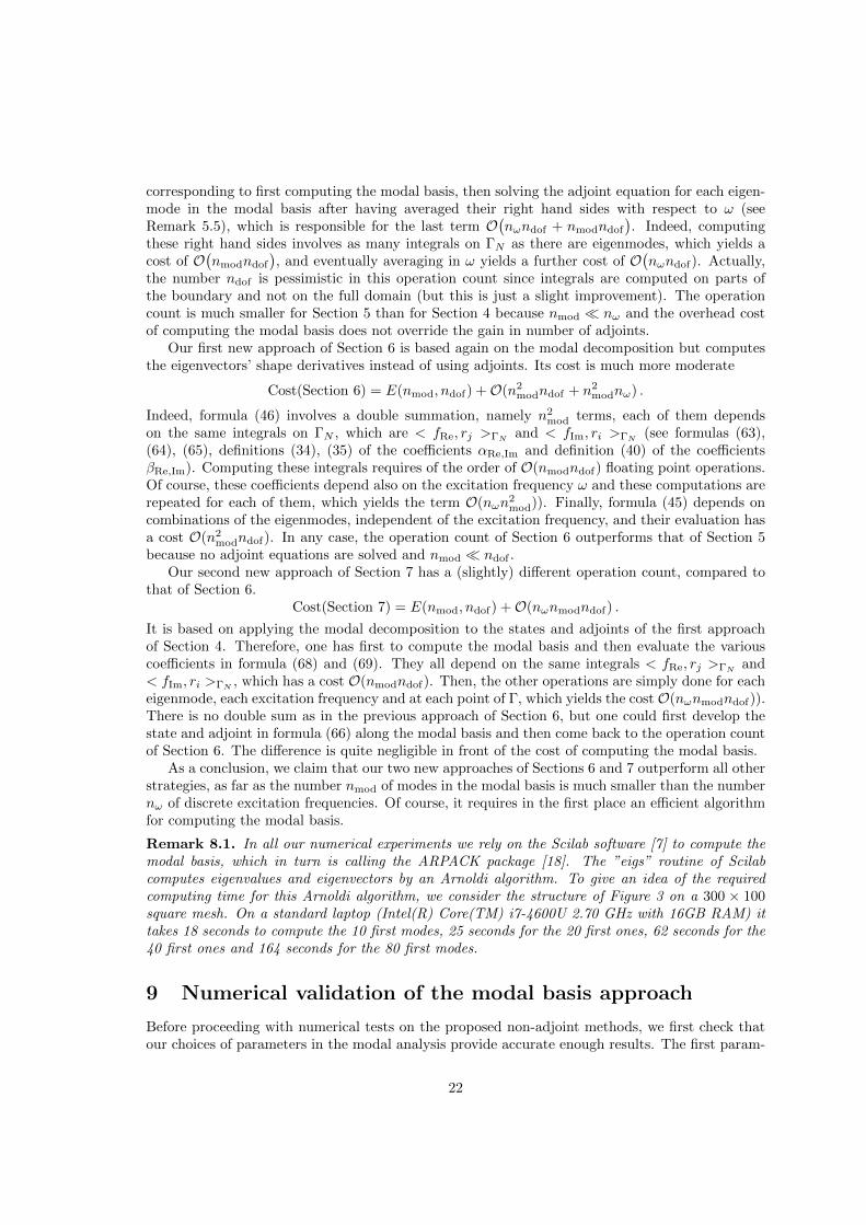
The optimized shapes for problem (73), using all three methods (of Sections 5, 6 and 7), fordifferent values of the upper bound coefficient α, appear in Figures 5, 6 and 7. The values of theobjective function and constraints, as well as the number of optimization iterations, are shown inTable 2. From these results, one can easily verify that none of the three methods outperformsthe others, both in terms of objective function value or total iteration numbers. Moreover, asexpected, all results correspond to local minima, which depend strongly on the initialization. Thisbecomes evident from the observation that the shape obtained using the modal decomposition ofthe eigenvectors’ shape derivative for α = 0.3 has lower volume than the optimized shape withoutconsidering the dynamic compliance. As a result, modifying the optimization parameters couldresult in another local optimum. For example, compared to the optimized shape of Figure 6 (up),constraining the maximum number of transport iteration steps for the level-set function to the

27

half results in another optimized shape, shown in Figure 8. The performance of this new shapeis slightly better than previsouly (V (Ω) = 0.431,C(Ω) = 148.19,Cdyn(Ω) = 10.21), however itrequires more iterations to converge (46 iterations instead of 33 previously).

Figure 5: Optimized MBB beam for problem (73) setting: α = 0.70 (up); α = 0.50 (middle);α = 0.30 (down), using the adjoint method of Section 5.

Figure 6: Optimized MBB beam for problem (73) setting: α = 0.70 (up); α = 0.50 (middle);α = 0.30 (down), using the modal decomposition of eigenvectors’ shape derivative of Section 6.

28

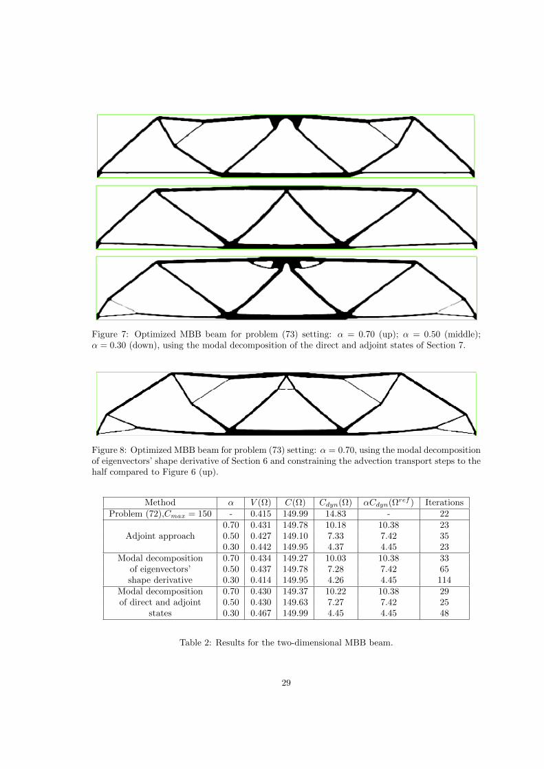
Figure 7: Optimized MBB beam for problem (73) setting: α = 0.70 (up); α = 0.50 (middle);α = 0.30 (down), using the modal decomposition of the direct and adjoint states of Section 7.

Figure 8: Optimized MBB beam for problem (73) setting: α = 0.70, using the modal decompositionof eigenvectors’ shape derivative of Section 6 and constraining the advection transport steps to thehalf compared to Figure 6 (up).

Method α V (Ω) C(Ω) Cdyn(Ω) αCdyn(Ωref ) IterationsProblem (72),Cmax = 150 - 0.415 149.99 14.83 - 22

0.70 0.431 149.78 10.18 10.38 23Adjoint approach 0.50 0.427 149.10 7.33 7.42 35

0.30 0.442 149.95 4.37 4.45 23Modal decomposition 0.70 0.434 149.27 10.03 10.38 33

of eigenvectors’ 0.50 0.437 149.78 7.28 7.42 65shape derivative 0.30 0.414 149.95 4.26 4.45 114

Modal decomposition 0.70 0.430 149.37 10.22 10.38 29of direct and adjoint 0.50 0.430 149.63 7.27 7.42 25

states 0.30 0.467 149.99 4.45 4.45 48

Table 2: Results for the two-dimensional MBB beam.

29

10.2 Two-dimensional cantilever

The second example is a two-dimensional 2x1 cantilever, discretized by 200x100 Q1 elements,clamped at its left boundary and with a unit vertical force applied at the middle of its right side(see Figure 9). The initialization and the optimized shape for problem (72) (without the dynamiccompliance), choosing Cmax = 170, appear in Figure 10. It will serve as the reference shape in thesequel.

Figures 11, 12 and 13 show the optimized shapes for problem (73) for all three methods anddifferent values of α. The vibrating force is of the same type as previously and the excitationfrequency belongs to the interval ω ∈ [0.1, 0.3] Hz. The reference value for the dynamic complianceequals Cdyn(Ωref ) = 57.40. More details about these results are presented in Table 3.

Figure 9: Boundary conditions for the two-dimensional cantilever.

Figure 10: Left: initialization; right: optimized shape for the static compliance problem (72).

Figure 11: Optimized cantilever for problem (73) setting: α = 0.70 (left); α = 0.50 (middle);α = 0.30 (right), using the adjoint method of Section 5.

30

Figure 12: Optimized cantilever for problem (73) setting: α = 0.70 (left); α = 0.50 (middle);α = 0.30 (right), using the modal decomposition of eigenvectors’ shape derivatives of Section 6.

Figure 13: Optimized cantilever for problem (73) setting: α = 0.70 (left); α = 0.50 (middle);α = 0.30 (right), using the modal decomposition of the direct and adjoint states of Section 7.


0.70 0.092 169.70 39.99 40.18 37Adjoint 0.50 0.096 169.77 28.41 28.70 112

0.30 0.103 169.99 17.22 17.22 115Modal decomposition 0.70 0.092 169.85 39.27 40.18 16

of eigenvectors’ 0.50 0.094 169.92 27.71 28.70 22shape derivative 0.30 0.115 168.94 15.43 17.22 35


states 0.30 0.120 169.53 16.70 17.22 70

Table 3: Results for the two-dimensional cantilever.

10.3 Three-dimensional bridge

The first three-dimensional example is a 6x1x1 bridge-like structure. The displacement is fixedat the two lower-right corners and the vertical displacement is fixed at the opposite corners. A

uniform pressure load q is applied at the top of the bridge such that

∫ΓN

q ds = 100. The boundary

conditions are shown in Figure 14. Due to symmetry, only one quarter of the structure is consideredand discretized by a 60 × 20 × 10 uniform hexaedral mesh. The solution of the elasticity andeigenvalue problems is performed in FreeFem++, by splitting each cubic element of the mesh into6 tetrahedra [12].

The optimized shape for problem (72) and Cmax = 7510250 is displayed on Figure 15. Then,multipying this pressure load q by a vibrating amplitude cos(ωt) in the frequency interval ω ∈

31

[0.03, 0.08] Hz, we solve problem (73) with a bound on the dynamic compliance with respect tothe reference structure of Figure 15, for which Cdyn(Ωref ) = 186358. For this test case, we useonly the method of Section 7 which is based on the modal decomposition of the direct and adjointstates. For different values of α, the optimized shapes appear in Figures 16, 17 and 18. Moredetails for these results are presented in Table 4.

Figure 14: Boundary conditions for the three-dimensional bridge.

Figure 15: Optimized bridge for the static compliance problem (72).

32

Figure 16: Optimized bridge for problem (73) setting α = 0.70, using the modal decomposition ofthe direct and adjoint states.

33

Figure 17: Optimized bridge for problem (73) setting α = 0.50, using the modal decomposition ofthe direct and adjoint states.

34

Figure 18: Optimized three-dimensional bridge for problem (73) setting α = 0.30, using the modaldecomposition of the direct and adjoint states.

Method α V (Ω) C(Ω) Cdyn(Ω) αCdyn(Ωref ) IterationsProblem (72),Cmax = 7510250 - 0.162 7479060 186358 - 49

Modal decomposition 0.70 0.169 7506030 125195 130451 80of direct and adjoint 0.50 0.174 7469840 91248 93179 44

states 0.30 0.167 7483880 51436 55907 58

Table 4: Results for the three-dimensional bridge.

10.4 Three-dimensional cantilever

The last test-case is a three-dimensional cantilever, clamped at its left side and with a unit verticalload applied in the middle of its right side (see Figure 19). Due to symmetry with respect to they-axis, only half of the domain is used and discretized by 60× 15× 30 hexaedra.

The optimized shape for problem (72) and Cmax = 80 is shown in Figure 20. Then, solvingproblem (73) for different values of α, via the method of Section 7 (based on the modal decompo-sition of the direct and adjoint states), yields the optimized shapes of Figures 21, 22 and 23. Thevibrating force is again the static load multiplied by cos(ωt) in the excitation frequency intervalω ∈ [0.1, 0.3] Hz. The value of the reference dynamic compliance is Cdyn(Ωref ) = 18.41. Table 5contains the results for these shapes.

35

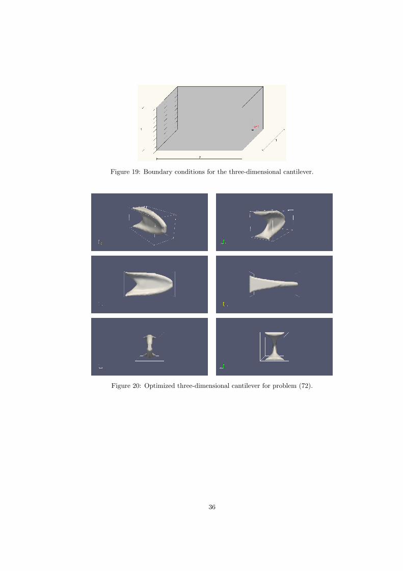
Figure 19: Boundary conditions for the three-dimensional cantilever.

Figure 20: Optimized three-dimensional cantilever for problem (72).

36

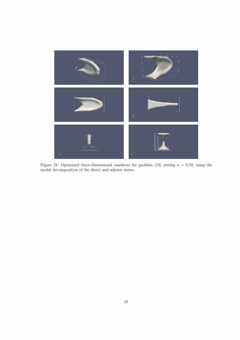
Figure 21: Optimized three-dimensional cantilever for problem (73) setting α = 0.70, using themodal decomposition of the direct and adjoint states.

37


38




states 0.30 0.167 79.95 5.38 5.52 81

Table 5: Results for the three-dimensional cantilever.

10.5 Double eigenvalues

In order to test the non-sensitivity of the method with respect to the existence of multiple eigenval-ues (see Remark (7.2)), we consider again the previous cantilever and we add a second load-case,similar to the first one, but with the external force oriented towards the y-axis. We discretizethe full-domain via a 40× 20× 20 hexaedral mesh and we do not use any symmetry assumption.Starting from a full-domain initialization and solving the optimization problem:

minΩ∈Uad

V (Ω)

s.t. C1(Ω) =

∫ΓN

g1 · u ds ≤ Cmax

C2(Ω) =

∫ΓN

g2 · u ds ≤ Cmax

(74)

39

for Cmax = 250, g1 = [0, 0, 1] and g2 = [0, 1, 0] results in the optimized shape of Figure 24. Theoptimized shape has kept its symmetry with respect to the y and z−axis and thus contains at leastone eigenvalue of multiplicity greater than one.

Adding a dynamic frequency constraint for each of the vibrating forces g1 cos(ωt) and g2 cos(ωt),in the excitation frequency interval ω ∈ [0.1, 0.3] Hz, we solve the optimization problem:

minΩ∈Uad

V (Ω)

s.t. C1(Ω) =

∫ΓN

g1 · u ds ≤ Cmax

C2(Ω) =

∫ΓN

g2 · u ds ≤ Cmax

C1dyn(Ω) ≤ αCdyn(Ωref )

C2dyn(Ω) ≤ αCdyn(Ωref )

(75)

for α = 0.3 and Cdyn(Ωref ) = 51.17. The optimized shape is shown in Figure 25 and the corre-sponding results in Table 6. Finally, the convergence diagrams for the objective function and theconstraints are shown in Figure 26 and the evolution of the first ten eigenfrequencies is plotted inFigure 27.

Clearly there are several double eigenvalues. The first and second eigenvalues, as well as theeighth and ninth remain double all along the optimization history. The fifth and sixth eigenvaluesare double in the beginning of the optimization, but after the third iteration a crossing occurs andits the fourth and fifth eigenvalues that continue as double. However, the existence of multipleeigenvalues does not seem to cause any trouble in the convergence of the optimization as can bechecked on the convergence history of Figure 26.

Figure 24: Optimized three-dimensional cantilever for problem (74).

40


Method α V (Ω) C1(Ω) C2(Ω) C1dyn(Ω) C2

dyn(Ω) αCdyn(Ωref ) Iterations

Problem (72),Cmax = 250 - 0.620 249.493 249.493 51.17 51.17 - 13Modal decompositionof direct and adjoint 0.30 0.626 249.763 249.770 15.254 15.242 15.351 17

states

Table 6: Results for the three-dimensional cantilever of figures 24 and 25.

Acknowledgements

The authors acknowledge fruitful discussions and helpful remarks from Marc Albertelli (Renault).The first author G.A. is a member of the DEFI project at INRIA Saclay Ile-de-France. This workstarted while the second author G.M. was a research engineer at CMAP, Ecole Polytechnique,financially supported by the Institut Carnot.

References

[1] G. Allaire. Conception optimale de structures, volume 58 of Mathematiques & Applications.Springer-Verlag, Berlin, 2007.

[2] G. Allaire, F. Jouve, and A.-M. Toader. A level-set method for shape optimization. C. R.Acad. Sci. Paris, Serie I, 334:1125–1130, 2002.

[3] G. Allaire, F. Jouve, and A.-M. Toader. Structural optimization using sensitivity analysis anda level-set method. Journal of computational physics, 194(1):363–393, 2004.

[4] O. Amir, N. Aage, and B. Lazarov. On multigrid-cg for efficient topology optimization.Structural and Multidisciplinary Optimization, 49(5):815–829, 2014.

41

Figure 26: Convergence diagrams for the volume (up), the compliance (midle) and the dynamiccompliance (down) for the results of Figure 25.

[5] M.P. Bendsoe and O. Sigmund. Topology optimization: theory, methods and applications.Springer, 2004.

[6] H. Brezis. Functional analysis, Sobolev spaces and partial differential equations. Universitext.Springer, New York, 2011.

[7] S. L. Campbell, J.-Ph. Chancelier, and R. Nikoukhah. Modeling and simulation in

42

Scilab/Scicos. Springer, New York, 2006.

[8] J. Cea. Conception optimale ou identification de formes: calcul rapide de la derivee direction-nelle de la fonction cout. Modelisation mathematique et analyse numerique, 20(3):371–402,1986.

[9] P.W. Christensen and A. Klarbring. An introduction to structural optimization, volume 153.Springer, 2009.

[10] R.W. Clough and J. Penzien. Dynamics of structures. McGraw-Hill Book Co., New York,1975.

[11] P.D. Dunning and H.A. Kim. Introducing the sequential linear programming level-set methodfor topology optimization. Structural and Multidisciplinary Optimization, 51(3):631–643, 2015.

[12] P. Frey and H. Borouchaki. Texel: triangulation de surfaces implicites(partie ii, exemplesd’applications). Rapports de recherche- INRIA, 1997.

[13] F. Hecht. New development in freefem++. J. Numer. Math., 20(3-4):251–265, 2012.

[14] A. Henrot and M. Pierre. Variation et optimisation de formes: une analyse geometrique,volume 48. Springer, 2005.

[15] J.S. Jensen. Topology optimization of dynamics problems with pade approximants. Interna-tional Journal for Numerical Methods in Engineering, 72(13):1605–1630, 2007.

[16] C.S. Jog. Topology design of structures subjected to periodic loading. Journal of Sound andVibration, 253(3):687–709, 2002.

[17] T. Kato. Perturbation theory for linear operators, volume 132 of Grundlehren der Mathema-tischen Wissenschaften. Springer Verlag, 1980.

[18] R. B. Lehoucq, D. C. Sorensen, and C. Yang. ARPACK users’ guide, volume 6 of Software,Environments, and Tools. Society for Industrial and Applied Mathematics (SIAM), Philadel-phia, PA, 1998.

[19] Z.-D. Ma, N. Kikuchi, and I. Hagiwara. Structural topology and shape optimization for afrequency response problem. Computational mechanics, 13(3):157–174, 1993.

[20] Zheng-Dong Ma, Noboru Kikuchi, and Hsien-Chie Cheng. Topological design for vibratingstructures. Comput. Methods Appl. Mech. Engrg., 121(1-4):259–280, 1995.

[21] S. Min, N. Kikuchi, Y.C. Park, S. Kim, and S. Chang. Optimal topology design of structuresunder dynamic loads. Structural optimization, 17(2-3):208–218, 1999.

[22] Jean-Claude Nedelec. Acoustic and electromagnetic equations, volume 144 of Applied Math-ematical Sciences. Springer-Verlag, New York, 2001. Integral representations for harmonicproblems.

[23] N. Olhoff and J. Du. Topological design for minimum dynamic compliance of continuumstructures subjected to forced vibration. Structural and Multidisciplinary Optimization, 2012.

[24] S.J. Osher and R. Fedkiw. Level set methods and dynamic implicit surfaces, volume 153 ofApplied Mathematical Sciences. Springer-Verlag, New York, 2003.

43

[25] S.J. Osher and F. Santosa. Level set methods for optimization problems involving geometryand constraints: I. frequencies of a two-density inhomogeneous drum. Journal of Computa-tional Physics, 171(1):272–288, 2001.

[26] S.J. Osher and J.A. Sethian. Fronts propagating with curvature-dependent speed: algorithmsbased on hamilton-jacobi formulations. Journal of computational physics, 79(1):12–49, 1988.

[27] J.A. Sethian. Level set methods and fast marching methods: evolving interfaces in com-putational geometry, fluid mechanics, computer vision, and materials science. Cambridgeuniversity press, 1999.

[28] J.A. Sethian and A. Wiegmann. Structural boundary design via level set and immersedinterface methods. Journal of computational physics, 163(2):489–528, 2000.

[29] L. Shu, M.Y. Wang, Z. Fang, Z. Ma, and P. Wei. Level set based structural topology optimiza-tion for minimizing frequency response. Journal of Sound and Vibration, 330(24):5820–5834,2011.

[30] J. Simon and F. Murat. Sur le controle par un domaine geometrique. Publication 76015 duLaboratoire d’Analyse Numerique de l’Universite Paris VI, (76015):222 pages, 1976.

[31] J. Soko lowski and J.-P. Zolesio. Introduction to shape optimization. Springer-Verlag, Berlin,1992.

[32] D. Tcherniak. Topology optimization of resonating structures using simp method. Interna-tional Journal for Numerical Methods in Engineering, 54(11):1605–1622, 2002.

[33] M.Y. Wang, X. Wang, and D. Guo. A level set method for structural topology optimization.Computer methods in applied mechanics and engineering, 192(1):227–246, 2003.

[34] G.H. Yoon. Structural topology optimization for frequency response problem using modelreduction schemes. Computer Methods in Applied Mechanics and Engineering, 199(25):1744–1763, 2010.

44

Figure 27: Evolution of the first 10 eigenfrequencies during the optimization process for the opti-mized shape of Figure 25 (top) and various zooms (bottom).

45

modal basis approaches in shape and topology optimization

Documents