mobility models for mobile ad hoc network simulations · mobility models for mobile ad hoc network...
TRANSCRIPT

Helsinki University of Technology
Department of Electrical and Communications Engineering
Networking Laboratory
Frans Wilhelm Bernhard Ekman
Mobility Models for Mobile Ad Hoc Network Simulations
Master’s Thesis submitted in partial fulfillment of the requirements for the degree of Master of Science in Technology.
May 15, 2008
Frans Ekman
Supervisor: Professor Jörg Ott
Instructor: Jouni Karvo, D. Sc. (Tech.)
Mobility Models for Mobile Ad Hoc Network Simulations
- I -
HELSINKI UNIVERSITY
OF TECHNOLOGY
ABSTRACT OF THE
MASTER’S THESIS
Author : Frans Wilhelm Bernhard Ekman
Title of the Thesis: Mobility Models for Mobile Ad Hoc Network Simulations
Date: May 15, 2008 Number of pages: 6+90
Department: Department of Electrical and Professorship: S-38
Communications Engineering
Supervisor: Professor Jörg Ott
Instructor : Jouni Karvo, D. Sc. (Tech.)
Delay-tolerant networks are characterized by opportunistic connectivity and long delays. A certain field of delay-tolerant networking focuses on sparsely populated ad hoc networks, where packets are routed in a store-and-forward manner. Many aspects of real world movement are not captured reliably in the simple movement models that are often used in delay-tolerant network simulations. Thus, approaches to create more realistic movement models are justified.
This master's thesis presents a movement model designed using a submodel approach. The model present the everyday life of average people that go to work in the morning, spend their day at work, do some activity with their friends in the evening and finally commute back to their homes. Movement takes place on a real world map, where nodes can move along roads. In addition to walking, public transportation and cars introduce more diverse movement patterns.
The model is validated by simulation and the statistical features of the model are compared to real world traces. Additional experiments are conducted to show the configurability of the model and the impact of the parameters. Again, statistical features are used for comparisons while simulation of the Epidemic routing protocol provides a ground for sensitivity analysis.
Keywords: Mobility Model, Simulation, Delay-Tolerant Network, DTN, Routing

Mobility Models for Mobile Ad Hoc Network Simulations
- II -
TEKNISKA HÖGSKOLAN
I HELSINGFORS
REFERAT OM
DIPLOMARBETE
Utfört av : Frans Wilhelm Bernhard Ekman
Arbetets namn: Rörelsemodeller för simulering av mobila ad hoc nätverk
Datum: 15 Maj 2008 Sidoantal: 6+90
Avdelning: Avdelning för elektro- och Professur: S-38
telekommunikationsteknik
Övervakare: Professor Jörg Ott
Handledare: Tekn.dr Jouni Karvo
Fördröjningstoleranta nätverk karaktäriseras av opportunistisk konnektivitet och långa fördröjningar. Ett delområde inom fördröjningstoleranta nätverk är glest befolkade ad hoc nätverk där paket vidarebefordras med hjälp av rörelsebaserad kommunikation. Ofta används mycket enkla rörelsemodeller i samband med simuleringar av dessa nätverk. Dessa enkla rörelsemodeller lämnar obeaktat ett flertal egenskaper som förekommer inom riktiga människors rörelsemönster. Det finns ett behov av en mera verklighetsnära rörelsemodell.
I det här diplomarbetet presenteras en rörelsemodell som bygger på mindre undermodeller. Modellen beskriver vardagligt liv för vanliga människor som går till sitt arbete på morgonen, arbetar hela dagen, tillbringar tid med sina bekanta efter arbetet och till sist tar sig tillbaka hem. Allting händer på en riktig karta där noder kan röra sig längs med vägar. Noder kan ta sig från ett ställe till ett annat genom att gå, åka bil eller använda sig av offentliga transportmedel, vilket ger upphov till mångsidigare rörelsemönster.
Modellens riktighet verifierades genom simulering och genom att jämföra modellens statistiska egenskaper med motsvarande egenskaper hos verkliga rörelsemönster. Rörelsemodellens konfigurerbarhet påvisas genom att undersöka olika parametrars inverkan. Detta görs också genom att jämföra ändringar inom statistiska egenskaper. Dessutom simuleras vägvals protokollet Epidemic för att visa hur sensitiv modellen är för ändringar i olika parametrar.
Nyckelord: Rörelsemodell, Simulering, Fördröjningstoleranta nätverk, Vägval

Mobility Models for Mobile Ad Hoc Network Simulations
- III -
Preface
This Master's Thesis has been done to the Networking Laboratory of the Helsinki University of Technology, within the SINDTN project which was funded by Nokia Research Center.
I thank my supervisor, Professor Jörg Ott, for all his support and for giving me the opportunity to write my thesis on such an interesting topic.
I want to express my gratitude to my instructor, Dr. Jouni Karvo, for all the insightful conversations we had during the project and for all the helpful comments on my text.
I would like to thank all my colleagues who have helped me with various things or provided me with knowledge in specific areas, especially: Ari Keränen, Niklas Beijar, Teemu Kärkkäinen and Tuomo Hyyryläinen.
Finally, I want to thank my parents for their support during my studies and my fiancée for her patience during the most stressful times.
May 15, 2008, in Espoo, Finland
Frans Ekman

Mobility Models for Mobile Ad Hoc Network Simulations
- IV -
PREFACE ............................................................................................................................................... III
ABBREVIATIONS................................................................................................................................. VI
1 INTRODUCTION............................................................................................................................1
1.1 AIMS AND SCOPE OF THIS WORK................................................................................................2 1.2 THE STRUCTURE OF THE THESIS.................................................................................................2
2 AD HOC NETWORKS AND SIMULATION...............................................................................3
2.1 AD HOC AND DELAY-TOLERANT NETWORKS.............................................................................3 2.2 ROUTING PROTOCOLS................................................................................................................4 2.3 SIMULATION ..............................................................................................................................5 2.4 SUMMARY .................................................................................................................................6
3 MOBILITY MODELS ....................................................................................................................7
3.1 CHARACTERIZATION OF CONTACTS...........................................................................................7 3.1.1 Inter-contact times...............................................................................................................7 3.1.2 Contact times .......................................................................................................................8
3.2 REAL USER TRACES...................................................................................................................8 3.2.1 Sources of real user traces...................................................................................................8 3.2.2 Insights from studying traces...............................................................................................8 3.2.3 Extracting a model from traces............................................................................................9 3.2.4 Limitations of real user traces .............................................................................................9
3.3 SYNTHETIC MODELS................................................................................................................10 3.3.1 Random walk .....................................................................................................................11 3.3.2 Random waypoint ..............................................................................................................12 3.3.3 Levy-Walk ..........................................................................................................................13 3.3.4 Map Based Movement........................................................................................................13 3.3.5 Shortest Path Map Based Movement .................................................................................14 3.3.6 Community based model....................................................................................................15 3.3.7 Time-variant mobility model..............................................................................................15 3.3.8 Indoor movement ...............................................................................................................16 3.3.9 Group movement................................................................................................................16 3.3.10 Problems and limitations ..............................................................................................16
3.4 SUMMARY ...............................................................................................................................16
4 DEVELOPING A SYNTHETIC MODEL ..................................................................................17
4.1 REQUIREMENTS.......................................................................................................................17 4.1.1 Group movement and contact durations............................................................................17 4.1.2 Inter-contact times.............................................................................................................18 4.1.3 Routines .............................................................................................................................18 4.1.4 Heterogeneity and Isolation...............................................................................................18 4.1.5 Social relationships ...........................................................................................................18 4.1.6 Synchronization .................................................................................................................18 4.1.7 Less movement ...................................................................................................................19 4.1.8 Overcome the boundary effect ...........................................................................................19
4.2 WORKING DAY MOVEMENT MODEL.......................................................................................20 4.2.1 Home activity submodel.....................................................................................................20 4.2.2 Office activity submodel.....................................................................................................21 4.2.3 Evening activity submodel .................................................................................................21 4.2.4 Transport submodel ...........................................................................................................22 4.2.5 The map .............................................................................................................................23
4.3 IMPLEMENTATION INTO THE ONE...........................................................................................24 4.3.1 ExtendedMovement class...................................................................................................26

Mobility Models for Mobile Ad Hoc Network Simulations
- V -
4.3.2 WorkingDayMovement and aggregate classes ..................................................................27 4.3.3 BusMovement class............................................................................................................32
4.4 SUMMARY ...............................................................................................................................33
5 EXPERIMENTAL SETUP ...........................................................................................................34
5.1 RECORDED METRICS...............................................................................................................34 5.1.1 Inter-contact times and contact durations .........................................................................34 5.1.2 Unique encounters, total encounters and their comparison ..............................................35 5.1.3 Number of contacts between two contacts with a node......................................................36 5.1.4 Hourly activity ...................................................................................................................36 5.1.5 Performance of the Epidemic routing protocol .................................................................36
5.2 SCENARIO SETTINGS................................................................................................................38
6 RESULTS .......................................................................................................................................41
6.1 VALIDATION OF THE MODEL....................................................................................................41 6.2 EXPLORING THE PARAMETER SPACE........................................................................................44
6.2.1 Density of nodes.................................................................................................................44 6.2.2 Use of buses or cars...........................................................................................................46 6.2.3 Use of districts ...................................................................................................................49 6.2.4 Use of a specific map.........................................................................................................51 6.2.5 Number of offices...............................................................................................................53 6.2.6 Office Size..........................................................................................................................55 6.2.7 Wait times inside office......................................................................................................57 6.2.8 Probability to do evening activity......................................................................................61 6.2.9 Evening activity group size................................................................................................63 6.2.10 Evening activity pause time...........................................................................................64 6.2.11 Use of SPMBM..............................................................................................................65 6.2.12 Differences in schedules................................................................................................68 6.2.13 Work times ....................................................................................................................70
6.3 SUMMARY ...............................................................................................................................71
7 DISCUSSION .................................................................................................................................72
7.1 MAJOR FINDINGS.....................................................................................................................72 7.2 CONFIGURATION .....................................................................................................................73 7.3 GENERATING CONFIGURATIONS..............................................................................................74 7.4 LIMITATIONS OF THE MODEL...................................................................................................74
7.4.1 Buildings and dimensions ..................................................................................................74 7.4.2 Traffic ................................................................................................................................75 7.4.3 Implementation ..................................................................................................................75
7.5 LIMITATIONS OF THE RESULTS.................................................................................................76 7.6 SUMMARY ...............................................................................................................................77
8 CONCLUSIONS ............................................................................................................................78
8.1 FUTURE WORK.........................................................................................................................78 8.2 FINAL WORDS..........................................................................................................................79
REFERENCES ........................................................................................................................................81
APPENDIX A: THE CONFIGURATION FILE OF THE DEFAULT S CENARIO ........................85

Mobility Models for Mobile Ad Hoc Network Simulations
- VI -
Abbreviations
AODV Ad Hoc On Demand Distance Vector
CCDF Complementary Cumulative Distribution Function
DTN Delay-Tolerant Networking
GPS Global Positioning System
GUI Graphical User Interface
MBM Map Based Movement
NS2 Network Simulator 2
OLSR Optimized Link State Routing
ONE Opportunistic Network Environment
PDA Personal Digital Assistant
RW Random Walk
RWP Random Waypoint
SPMBM Shortest Path Map Based Movement
TTL Time-To-Live
WDM Working Day Movement
WKT Well Known Text
WLAN Wireless Local Area Network

Mobility Models for Mobile Ad Hoc Network Simulations
- 1 -
1 Introduction
The number of wireless devices has increased drastically during the last decade. Most of the devices are only using existing network infrastructure for communication, even though in some scenarios the current technologies allow for direct communication between nearby devices. Ad hoc networks — formerly only used in military applications — are infrastructure-less networks where self-configuring devices are acting as routers and forming a network themselves. These devices and the entities carrying them are generally referred to as nodes in the literature.
Delay-Tolerant Networks (DTN) are more extreme environments, where lack of end-to-end connectivity requires nodes to carry packets a certain time before the packets can be forwarded to other nodes closer to the destination. Ideas for using ad hoc networks and DTN technologies for various consumer applications, or in hope of extending the connectivity to areas where no network infrastructure exists, have recently gained more popularity among researchers.
The design of applications and protocols for these environments often involves simulation. Various studies [1] have shown that user movement patterns are affecting the performance of protocols and applications highly; therefore, in order to get meaningful results, it is important to accurately model real usage scenarios with a model depicting movement at the level of individual devices.
Currently, too simple models are often used due to ease of implementation and configuration. Some of these models are able to produce statistically accurate distributions of events in terms of a few selected metrics. However, by looking at a lower level of abstraction, it is possible to see that certain real world characteristics are missing. It is not obvious which details are vital for acceptable results in DTN simulations and with which degree of abstraction the details can be modeled. Hence, there is a need for a movement model covering several different details that can in addition to simulation be used for studying the impact of different movement properties.

Mobility Models for Mobile Ad Hoc Network Simulations
- 2 -
1.1 Aims and scope of this work We present a new movement model to be used in DTN simulations, called the Working Day Movement Model. The model presents the everyday life of average people that go to work in the morning and, spend their day at work, and commute back to their homes at evenings. The model intuitively depicts the movement pattern of people.
The two objectives are:
I. The main objective of this thesis is to design and implement an extendable, configurable and well parameterized movement model for city scenarios. The model is verified by simulating it and comparing certain statistical features of the model to real world data.
II. The second objective is to study the impact of the parameters and determine how well the model can be configured for specific environments.
The scope of this work is limited to modeling of user movement within a city. Additionally, the movement model is limited to DTNs in the sense that the model is designed and validated against DTN specific criteria.
1.2 The structure of the thesis The structure of the remaining thesis is as follows: Chapter 2 provides some background information of ad hoc and delay-tolerant networks. Existing routing protocols, and development and simulation of new ones are discussed briefly. Chapter 3 discusses different approaches of modeling user movement in simulations.
Chapter 4 introduces our movement model. First the requirements of the model are presented, following with a description of the actual model in detail, and finally the implementation of the model is explained. Chapter 5 describes the experimental setup for the simulations, in addition to measurement methodologies and collected metrics.
Chapter 6 compares results from simulations of our model to real world measurements. Additionally, the impact of different parameters of the model is studied. Chapter 7 discusses the most important results, following with the limitations of the model and the limitations of the experiments. Finally, chapter 8 concludes the thesis and suggests ideas for future work.

Mobility Models for Mobile Ad Hoc Network Simulations
- 3 -
2 Ad hoc networks and simulation
In this chapter, we describe ad hoc and delay-tolerant networks in general. Additionally, we give some insight into routing in delay-tolerant networks, and finally discuss simulation of new applications and protocols.
2.1 Ad hoc and Delay-tolerant networks Ad hoc networks are infrastructure-less networks formed by self-configurable nodes where each node can act as a router itself. Ad hoc networks have been common in military applications where vehicles or other troops need to be able to communicate with each other in the battlefield. Other applications include different sensor networks where nodes have very limited resources, but are not limited to small low-capacity devices. Packets are delivered from the source node to the destination node through a link formed by intermediary nodes. Different routing protocols have been developed for finding the optimal route.
In some more extreme environments, end to end connectivity does not exist at all times. In these situations packets need to be routed in a store and forward way, i.e. intermediary nodes need to carry packets until they get an opportunity to forward them. These networks are often called opportunistic networks or Delay-Tolerant Networks (DTN), and require a different set of solutions to address the problem of lack of end to end connectivity.
Different types of DTNs exist in different environments. Jones et al [2] characterize DTNs by contact schedules, contact capacity, buffer space, processing power and energy. Contact schedules can either be predictable or unpredictable. A good example of a DTN with predictable contact schedules is scenarios in deep space where the routes of satellites or other spacecraft are predetermined. In many other environments the contact schedules are unpredictable, for example: humans moving while carrying their mobile devices. Many environments are something in between, where only statistical information about the schedules is available. The contact capacity, together with the duration of the contact between two nodes, determines the amount of data that can be exchanged. Similarly, the amount of buffer space limits the amount of data that can be stored and carried by devices. When dealing with wireless devices, processing power and energy consumption must almost always be taken into account.

Mobility Models for Mobile Ad Hoc Network Simulations
- 4 -
Common networking technology practices cannot always be applied directly to DTNs. Conversational protocols with many round trips required for message transfers to complete are usually not suitable for DTNs. In DTNs it is better to design protocols to require as few transactions as possible between the source and the destinations. An architecture for DTNs is proposed in [3], where messages are transferred in bundles, above the transport layer.
2.2 Routing protocols Protocols such as OLSR (Optimized Link State Routing) [4] and AODV (Ad hoc On-Demand Distance Vector) [5] are commonly used in traditional ad hoc networks, where end to end connectivity is assumed at all times. These protocols fail in DTNs due to connectivity problems [6]. Therefore, new routing protocols are needed which can operate in environments where nodes have to carry packets.
Jones et al. [2] classifies routing strategies by two properties; replication and knowledge. The former stands for making multiple copies of a messages and transferring them along different paths to increase the chance that the message gets through. This is a tradeoff between overhead and delay. The latter stands for how much knowledge about the network is required by the routing strategy. The paper distinguishes between two major strategies used for finding the destination; flooding strategies and forwarding strategies.
Flooding strategies are based on nodes distributing packets in tree-like way through the network. Different approaches exist to limit the tree-size by depth, breadth or total number of replicas allowed to be made of the original message. The Epidemic routing protocol is an extreme example of a flooding strategy. Each time two nodes are in contact with each other they exchange all the messages stored in their buffers unless prevented by bandwidth- or buffer capacity constraints. This approach consumes a lot of resources since the network gets quickly full, while copies of old packets that have already been delivered to their target continue to travel in the network. Different ideas to limit the resource consumption exist, for example the use of death certificates to inform nodes which packets have reached the destination and use of intelligent buffer management algorithms.
Forwarding strategies use network topology information to select the best path. Typically, one message is sent through this path without replication, requiring some knowledge for the protocols to operate. Location based routing is an idea to use geographical coordinates or some other topology information to determine which nodes are more likely to be closer to the destination. Gradient routing is an approach to assign weights to each node, where the weights are corresponding to a node’s suitability to deliver a message. Some knowledge must be propagated to all nodes in the beginning so that the weights can be calculated; otherwise a hybrid approach using random forwarding in the beginning must be used. With complete knowledge about the schedules of the contacts between nodes, a modified version of Dijkstra’s shortest path algorithm can be used [7], which takes into account the time varying connectivity graph.
The most suitable routing algorithm depends on the nature of the applications, the use cases and the environment it is designed for. If we consider a DTN network of buses,
Mobility Models for Mobile Ad Hoc Network Simulations
- 5 -
having huge buffers and a high transmission speed where only small messages are sent very rarely, we might want to choose the Epidemic routing approach. On the other hand, in a city scenario where people have DTN modules on their mobile phones, the Epidemic routing protocol may fail due to limited resources on phones. Instead one may be able to utilize information about the social relationships between people (some people meet more often) or common locations where people spend most of their time. The movement of people is also different between cities, which can also affect the choice of algorithm. Different applications might as well have different criteria for latency, delivery ratio, etc.
When developing new protocols, it is rarely possible or affordable to try them out in practice immediately. Therefore, we usually want to simulate our idea to better be able to determine whether it is an idea worth to try out in practice. The next chapter discusses DTN simulations in more detail.
2.3 Simulation Simulations can rarely replace real experiments conducted in the target environment, but are usually the best way to try out new ideas in an affordable way. This is especially true in the case of DTNs with mobile phones in city scenarios. Purchasing enough phones and recruiting enough people to achieve the desired nodal density within a sufficiently large area is out of the question. However, it is possible to simulate a scenario like this with some statistical data about the movement of people.
There are plenty of both free and commercial simulation tools available for all kinds of different networks. The NS2 simulator1 is a general purpose simulator that can be used to some extent for DTN simulations, too. It has also been common within universities and other research institutes to develop own simulators for experiments. A Java based simulator, DTNSim2 has been developed at the University of Waterloo. The Networking Laboratory at Helsinki University of Technology has also developed an own GUI based simulator, the ONE (Opportunistic Network Environment) [8].
Like in all simulations, we want to model the target environment as closely as possible. However, we must create an abstraction, where many details have been disregarded, to maintain the complexity at a tolerable level. Which details to focus on depends completely on what we are simulating. A mobile network operator simulating a 3G network deployed in a new area might be mostly interested in how many devices are going to be connected to each cell during different hours. Therefore, it is important to model the amount of people within certain areas and the terrain which attenuates the signals. Hence, it may not be as important to model individual users and their lives in detail. However, for DTN simulations we are more interested to know about how nodes get in contact with each other, since it is during these contacts that packets get forwarded. The contacts are highly related to the locations nodes visit; therefore it is very important to model movement of nodes. In contrast to the 3G network simulations, it makes a difference where the nodes have been before they move to new areas.
1 http://www.isi.edu/nsnam/ns/ 2 http://watwire.uwaterloo.ca/DTN/sim/

Mobility Models for Mobile Ad Hoc Network Simulations
- 6 -
The contacts are also affected by other properties than mobility. The transmission range of the used technology determines how close nodes must be to each other to be in contact. Transmission speed and setup times will limit the amount of data that can be sent, and walls and other obstacles will attenuate the signal. Many nodes close to each other will also interfere.
It is common to create an abstraction encapsulating many of the details of the physical layer. One idea is to directly use data, containing timestamps and durations for all contacts between two nodes. This contact data is usually referred to as the contact trace. The contact trace can be synthetically generated or obtained from real world measurements. In either case, when a contact trace is used as input for the simulator, it is assumed that the contact trace constitutes the effect of walls and other details. However, the perceived bandwidth is usually not recorded in the trace, and a constant bandwidth is used later in the actual simulations.
Most of the protocols can be simulated with a pure contact trace; however, there are a few exceptions. Some protocols using GPS data or other knowledge to predict where to forward packets cannot be simulated without information about node locations. In these cases we need to remove one level of abstraction and capture node locations at given timestamps instead, which we call the movement trace. The modeling of user movement in simulations is more common, since the contact trace can always be derived from it.
2.4 Summary In this chapter we presented in brief how packets can be routed in a store and forward way in delay-tolerant networks. We discussed simulation of new protocols and modeling of the target environment. We concluded that the user movement patterns and the contacts between users are important to capture accurately in a model used for DTN simulations.

Mobility Models for Mobile Ad Hoc Network Simulations
- 7 -
3 Mobility models
As stated in the previous chapter, movement of the network nodes is essential for the performance of sparsely populated delay-tolerant networks, since end-to-end connectivity does not always exist and packets are delivered in a store and forward manner. Capturing movement accurately in the real usage scenarios is thus needed for a reliable assessment of a new protocol. Movement can be captured in simulations by either using real movement traces or synthetic traces generated by a movement model. This chapter describes both approaches.
3.1 Characterization of contacts When we simulate a new protocol, we can as well have just the contacts between nodes as input data instead of the movement of nodes. Of course this does not apply to routing protocols utilizing geographical location data, but most of the other protocols can be simulated with pure contact data. Therefore, it is very common to characterize mobility by the contacts, which are in fact connection opportunities. We have chosen to use two parameters, inter-contact times and contact times, to characterize the contacts, and we use the same definitions as in [9].
3.1.1 Inter-contact times An inter-contact time, or sometimes referred to as an inter-meeting time, is the time interval between contacts for a node pair. In other words, the time interval a node pair is not in contact. Inter-contact times correspond to how often nodes will have an opportunity to send packets to other nodes. We will work with distributions of inter-contact times, since the nature of the distribution has an impact on the performance of different routing protocols.
Chaintreau et al. [10] show that if the distribution of inter-contact times is power-law distributed with an exponent less than one, any possible routing algorithm in a delay tolerant network will produce an infinite average delay for packet delivery. In the same paper they have analyzed four different traces of real people moving, and concluded that the inter-contact times are power-law distributed with an exponent less than one. This is bad in scenarios where we assume that the communicating node pairs are arbitrarily selected from the set of all nodes, i.e. a situation where each node is equally

Mobility Models for Mobile Ad Hoc Network Simulations
- 8 -
likely to send a message to any other specific node. But in practice it is likely that the communication need between nodes is distributed in such a way that it reflects social networks in real life or other aspects; therefore, a finite average delay is still possible.
Other studies [11] show that the inter-contact times are only power-law distributed up to 12 hours, and follow an exponential distribution after that. A possible cause for the phenomenon is the daily routines people have. In many cases it is not easy to say whether there is an exponential decay or if it’s just systematic error that comes from the way inter-contact times were measured in the experiments.
3.1.2 Contact times The contact time or contact duration is the time a contact lasts. The contact durations correspond to the limit of data can be sent during a contact. In sparsely populated networks, the interference of other nearby nodes will be insignificant; hence, the duration of the contact determines the amount of data that can be sent. We also measure the contact time distribution.
3.2 Real user traces The most realistic user movement or contact patterns are the ones that happen in the real world. Therefore, several studies have focused on tracking user movement to be able to use the traces later directly for simulations or to learn more about which characteristics are common in real user behavior. There are two types of user traces that have been collected in different experiments — contact traces containing timestamps when node pairs have been in contact and movement traces containing the locations of nodes at given timestamps.
3.2.1 Sources of real user traces Movement traces have usually been obtained by analyzing WLAN access point data or having users carry around devices equipped with GPS modules. Contact traces have mostly been collected from real world experiments where users have been carrying around Bluetooth devices tracking other devices within range.
Chaintreau et al. [9] analyzed WLAN access point data sets from UCSD [12] and Dartmouth [13] and recreated movement traces from them. They assumed that two nodes connected to the same access point at the same time are in contact with each other. Additionally, they conducted their own experiments with small Bluetooth devices called iMotes. In these experiments, a group of people were carrying iMotes, which scanned for other devices every two minutes. During the period between the scans, the devices were able to respond to inquiries from other devices. The iMote devices recorded contacts both with other iMote devices and any other Bluetooth devices. The result was a contact trace. We use the same contact trace [14] for validation of our model later in this study.
3.2.2 Insights from studying traces Studying traces can reveal new characteristics and statistical properties of mobility that can be used in the development of new DTN routing protocols and applications. Data from these analyses is also important when modeling a specific environment. As we
Mobility Models for Mobile Ad Hoc Network Simulations
- 9 -
already mentioned, the nature of the distribution of inter-contact times and contact durations play a huge role in the performance of protocols. Therefore it is of great interest for protocol developers to have statistical data about both of these. Moreover, simulations need mobility models unless real user traces are used. To be able to develop better mobility models it is crucial to have a good understanding of what realistic user movement is.
3.2.3 Extracting a model from traces A common approach in development of new mobility models is to extract a synthetic model from real user traces. The idea is to come up with a model and then estimate the parameters from the traces. For example, it is possible to statistically determine various parameters and their distributions, like the pause time, speed, etc.
Kim et al [15] extracted various parameters such as speed and pause time distributions from real user traces. These parameters were then used in a synthetic mobility model. Their model is validated based on the number of nodes within different regions on the map at different hours. This might not be a sufficient criterion alone to determine the suitability of a model, since the performance of protocols and applications in DTN is highly related to the nature of the contacts.
3.2.4 Limitations of real user traces The idea of directly using the collected traces in simulations sounds very tempting at fist, but there are, however, a few drawbacks. The traces are usually from very specific environments like campus areas so they do not capture movement within other environments like cities. Movement patterns within a campus area can be very different than in the center of a city. The collected data sets also have certain limitations, explained in the following sections.
Movement traces Movement traces are often measured in places where only certain areas have WLAN coverage; hence, nodes meeting outside access points do not get recorded. Additionally, the approach is not so accurate because nodes within the same access point might not be in reach of each other.
When the locations of users are derived from access point data, the result is roughly building level granularity [16]. This is because users are not always connected to the closest access point and the movement between access points is difficult to capture.
Most of the devices connecting to WLAN access points in these experiments are laptops and PDAs which are not always carried by the users and are not necessarily always turned on. Whether this characteristic is wanted in the simulations depends on what is modeled and simulated. Paper [10] argues that the on/off times are an important characteristic of wireless users that needs to be taken into account and modeled for simulations. In our experiments we are more interested to model a city environment where users are carrying always-on wireless devices where all are supporting the same routing protocols. Whether this is practical and technically feasible due to short battery lifetime and other issues is a topic for another discussion.

Mobility Models for Mobile Ad Hoc Network Simulations
- 10 -
Even though we accept these weaknesses, we still have to deal with nodes leaving the simulation area. Nodes entering the simulation area may be carrying arbitrary packets depending on their movement and connections outside the area. This introduces other problems.
Contact traces We mentioned earlier that contact traces are not always sufficient because they do not contain any location data. Location data is usually not necessary in simulations but a bigger problem with most contact traces is the fact that only certain parts of the connectivity graph are recorded. For example, the iMote traces only contain connections between two iMote devices and connections between an iMote and anoter Bluetooth device. Connections between any two other devices can obviously not get recorded. This limited connectivity graph is not sufficient for reliable simulations.
Other considerations It is also practical to have a model with configurable parameters to work with. Sometimes a protocol or an application developer wants to test how the protocol or application performs when certain parameters change, to better be able to find out weaknesses and strengths. Sometimes researchers also need a very simple model to work with, to be able to use it in mathematical proofs for various theorems.
3.3 Synthetic models Synthetic models are often preferred since they are easier to work with than real user traces. Moreover, real user traces are rarely available for the environment to be modeled. Additionally, researchers want to do sensitivity analysis to find out how protocols and applications perform under different conditions. This is not possible with real user traces unless a parameterized model has been successfully extracted. Pure mathematical models are also necessary for scientists to be able to prove various concepts [17].
There are two types of synthetic movement models that have been proposed for these analyses — generic high level models that aim to produce movement accurate enough with statistical measures, and models that describe incidental scenarios, hoping for a more accurate depiction of single devices.
While efficient to use in simulations, the high level models, such as Random Waypoint [18], often imply that the scenarios for which the protocols are simulated have huge numbers of nodes, so that the relevant protocol features are given statistically realistic distributions of events. For scenarios with few nodes, the differences between different usage scenarios become more significant. Thus, movement models that depict more precisely some specific types of movement are needed.
Traditionally, the approach to create a movement model has been to identify a certain characteristic of mobility and to create a mathematical model describing the movement at a high level. Such characteristics can be speed distribution, social relationships between nodes or favorite locations nodes will visit. These types of movement have

Mobility Models for Mobile Ad Hoc Network Simulations
- 11 -
very few details and the movement is homogeneous in the sense that every node is moving according to the same rule.
Another approach is to increase the realism by adding lot’s of details, with the belief that all small details will together add up as realistic movement. With an approach like this, the movement will be more heterogeneous since cars, buses and pedestrians move differently. The increasing complexity introduces a risk of overfitting the model, i.e. fitting a model more complex than there is data available to verify it. If we only verify a model by comparing the inter-contact times to real world measurements, we will see that several completely different models exist that produce the exact same distribution of inter-contact times.
Before we go any further, we introduce two new terms: locality and heterogeneity. By locality we mean the tendency of nodes spending most of their time within a small area. Thus, a movement model where each node’s movement is restricted to a small area has high locality. By heterogeneity, we mean different movement patterns and properties between nodes. Measuring heterogeneity in a specific context is not straightforward, but in our experiments we will later on talk about differences in contact patterns in terms of how often a node encounters new nodes compared to the fraction of earlier encountered nodes.
3.3.1 Random walk The Random Walk (Brownian motion) is one of the simplest movement models available, where every node follows the same rule to decide its next move, in a totally memory-less manner. The idea is that every node randomly chooses an angle and a speed, and walks in that direction either a constant time or a constant distance. A variation with variable distance is also common.
Interesting with the random walk is that it has certain real-world properties, even though the movement is far from the way humans are walking in the real world. One interesting property is the locality of the node locations. A node is less likely to walk longer ways from the starting location. This characteristic results in power-law distributed inter-contact times on a boundless simulation area [11]. Generally for models, Han Cai et al. [19] show that simple models on a boundless area can produce a power-law distribution of inter-contact times. Additionally, they show that the exponential cut-off is in many cases a side-effect of the bounded area. The motivation behind this is that nodes that would move over the edges on an infinite area are forced to stay within the area, thereby meeting other nodes sooner than they otherwise would and the number of long inter-contact times will be smaller.
We simulated the Random Walk movement in a scenario with 1000 nodes on a 8300×7300m2 sized plane for a time of 7·105s. The nodes where moving with speeds 0.5–1.5m/2 uniformly distributed. The transmit range was set to 10m, which is relatively common for Bluetooth devices. Immediately when two nodes were within 10m of each other they were considered to be in contact (no delay in terms of connection setup and scanning of devices). The distances were uniformly selected between 0–50m. Nodes did not pause between movements, since pausing is not a property of the model. Figure 1 shows that the Random Walk generates a distribution of inter-contact times much closer to a power-law than the Random Waypoint, which is

Mobility Models for Mobile Ad Hoc Network Simulations
- 12 -
described in the next section. A power-law appears as a straight line on a graph with log-log scale.
3.3.2 Random waypoint In the Random waypoint (RWP) movement model nodes choose a random location on the simulation area and walk there with the speed drawn from a uniform distribution with a minimum and maximum value. When the node has arrived, it will wait a random amount of time, and then continue with the same routine.
One feature of the RWP model is that when it has reached a steady state, the nodes are not uniformly distributed on the simulation area. This must be taken into account either by using a warmup time sufficient length for the model to reach a steady state, or place nodes on the simulation area on locations following the appropriate distribution.
A shortcoming with the model is that it takes a very long time for the nodal average speed to stabilize. If we have set the minimum speed to 0, the model will never reach a steady state since the average speed is constantly decreasing [20].
We simulated the RWP movement with the same parameters as the Random Walk, except that the wait times were uniformly distributed in [1, 3600]s. The speeds were uniformly distributed between 0.5 and 5m/s, to compensate for the lost time in pauses. Figure 1 shows the inter-contact times distribution compared to the Random Walk model.
100
102
104
10−2
10−1
100
P[X
> x
]
Time [s]
RWRWP
0 1 2 3 4 5
x 105
10−5
100
P[X
> x
]
Time [s]
RWRWP
Figure 1: Inter-contact times for Random Walk and RWP

Mobility Models for Mobile Ad Hoc Network Simulations
- 13 -
3.3.3 Levy-Walk Rhee et al. [21] studied several real world traces and concluded that the movement of real people from various outdoor settings and concluded that the movement follows a Levy-walk. The Levy-walk is an extension of the random walk, where the travelled distances follow a power law. The Levy-walk produces a power-law distribution of inter-contact times. However, it is arguable that it is not the Levy-walk that is behind the power-law distribution because random walk without bounds already produces such a distribution. It might be so that the Levy-walk just limits the movement even further, thereby minimizing the effect of the bounds. In other words; the world appears to be larger.
3.3.4 Map Based Movement The Map Based Movement (MBM) model is a mobility model included in the first release of the ONE. This movement model gets as input a map in the WKT (Well Known Text) format. The map consists of map points connected by links. All crossings are map points, and all curves in the roads are constructed by several links and map points.
The Map Based Movement works as follows: A mobile node moves by walking from one map node to the other by always randomly selecting one of the directly connected map nodes. In the first release of ONE, a mobile node was not allowed to choose the same map node it came from as its next waypoint. We changed it to be configurable since it plays a vital role in the shape of the distribution of the inter-contact times graph.
We conducted an experiment where we simulated MBM when nodes were allowed to move back and when they were not. We used the same parameters as we did in the RWP and Random Walk experiments in the previous sections. No pause times were used. The inter-contact times distribution is shown in Figure 2. An interesting observation from this experiment is that the less likely nodes are to travel long distances, the more power-law like will the distribution be.
100
102
104
10−2
10−1
100
P[X
> x
]
Time [s]
MBMMBM − Back allowed
Figure 2: Inter-contact times for Map Based Movement

Mobility Models for Mobile Ad Hoc Network Simulations
- 14 -
Another interesting observation is the effect of roads on the contact times. Because the space in which nodes are allowed to move in is restricted, it is more likely that two nodes walk along the same path for a longer time. To better understand the effect of the restricted space, we compared the distributions of contact durations from the MBM and Random Walk models. The result is shown in Figure 3. We observe that the map creates longer contacts. There are fewer choices the nodes can make when they come to a crossing, so two nodes are more likely to move along the same path.
100
101
102
103
10−2
100
P[X
> x
]
Time [s]
RWMBM
Figure 3: Contact-durations for MBM and RW
3.3.5 Shortest Path Map Based Movement The Shortest Path Map Based Movement (SPMBM) model also makes use of map data. The SPMBM and RWP models have certain similarities. Nodes select their next destination on the map by randomly selecting a map point on the map. The nodes will calculate the shortest path to the destination using Dijkstra’s algorithm. It is worth to note that the map points may not be uniformly distributed over the map. The number of map points depends on the construction of the map. An area where the roads have been constructed with many map points will more easily attract nodes. Therefore, it is possible that two maps of the exact same city, with the exact same streets, but obtained from different places, will produce different movement.
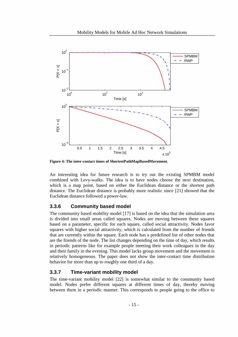
We conducted a similar experiment as we did for the MBM model in the previous section, with the same parameters except for the speed and wait time which were set to the same values as for RWP; 1–5m/s and 1–3600s, respectively. The inter-contacts times are presented in Figure 4. An interesting observation is that the inter-contact times are exponentially distributed like for the RWP.
Mobility Models for Mobile Ad Hoc Network Simulations
- 15 -
100
102
104
10−2
10−1
100
P[X
> x
]
Time [s]
SPMBMRWP
0.5 1 1.5 2 2.5 3 3.5 4 4.5
x 105
10−5
100
P[X
> x
]
Time [s]
SPMBMRWP
Figure 4: The inter-contact times of ShortestPathMapBasedMovement.
An interesting idea for future research is to try out the existing SPMBM model combined with Levy-walks. The idea is to have nodes choose the next destination, which is a map point, based on either the Euclidean distance or the shortest path distance. The Euclidean distance is probably more realistic since [21] showed that the Euclidean distance followed a power-law.
3.3.6 Community based model The community based mobility model [17] is based on the idea that the simulation area is divided into small areas called squares. Nodes are moving between these squares based on a parameter, specific for each square, called social attractivity. Nodes favor squares with higher social attractivity, which is calculated from the number of friends that are currently within the square. Each node has a predefined list of other nodes that are the friends of the node. The list changes depending on the time of day, which results in periodic patterns like for example people meeting their work colleagues in the day and their family in the evening. This model lacks group movement and the movement is relatively homogeneous. The paper does not show the inter-contact time distribution behavior for more than up to roughly one third of a day.
3.3.7 Time-variant mobility model The time-variant mobility model [22] is somewhat similar to the community based model. Nodes prefer different squares at different times of day, thereby moving between them in a periodic manner. This corresponds to people going to the office to

Mobility Models for Mobile Ad Hoc Network Simulations
- 16 -
work, to a restaurant to eat and home to sleep. The model is heterogeneous in both time and space. Nodes do not move in groups and the movement is homogeneous in the sense that every node follows the same instructions.
3.3.8 Indoor movement Little work has been made on indoor movement, especially combined with outdoor movement. Most of them are in a context not really practical for delay tolerant network simulations. Minder et al. [23] present a model for meetings where organization structure is taken into account. Nodes meet each other in team meetings of different lengths. The model is not so practical for DTN simulations because in practice people meet in corridors, work in the same room, etc. Habetha et al. [24] used a more detailed office movement model, where employees are moving in rooms and corridors. A model like this can produce accurate results if the office is modeled in detail with walls and rooms on their correct places.
3.3.9 Group movement Various group mobility models exist [25], for example the Reference Point Group Mobility model and the Overlap Mobility model. Analysis of the impact of people moving in groups has been made. However, to the best of our knowledge, group mobility has never been used in conjunction with another model. For example a community based model where nodes occasionally walk in a group together.
3.3.10 Problems and limitations Hsu and Helmy [26] show by studying real user traces that nodes are very often turned on/off and only visit a small portion of the WLAN access points in campus areas. Moreover, they find that node mobility while using network is very low and one node only meets a small portion of all other nodes in the area. These types of characteristics are usually not captured in movement models. Furthermore, they reveal repetitive patterns with a period of one day and heterogeneity among nodes. Although heterogeneity and repetitiveness has been modeled, most simple movement models do not. According to Hsu and Helmy, the biggest issue with most synthetic models is that they are not capturing such characteristics as heterogeneous behavior, switching devices on/off or relationships between users.
We noticed that even though most of the known features of movement have been modeled, no model exist where all or many of the features have been combined. Our approach is to combine these different elements to create a new movement model.
3.4 Summary We presented two metrics to characterize contacts, i.e. the inter-contact times and contact durations. Moreover, we discussed real world traces and their limitations. Finally, we described the most common movement models from previous research and provided some discussion about limitations of current movement models.

Mobility Models for Mobile Ad Hoc Network Simulations
- 17 -
4 Developing a synthetic model
We have created a synthetic model with many real world characteristics. We will first present the requirements of the model, i.e. properties that we believe are important to capture in the model. After that we will take a look at the model itself and provide a detailed explanation of its functionality. Finally, we go through the design and implementation of the model.
4.1 Requirements To keep complexity at a decent level, it is important to distinguish between more and less relevant mobility characteristics in a DTN context. It is not possible to know for sure which properties are important to capture, since we do not yet know how future DTN routing protocols are going to work and which characteristics have an impact on their performance; Therefore, we have based our requirements on combined ides from previous research with some own ideas included. Generally, our main requirement was to create a model with as many configurable real world properties as possible, so that the model can be used to derive almost any type of real world city scenario environment.
4.1.1 Group movement and contact durations In the real world, people often walk in groups and do various activities together, resulting in longer contact durations. Additionally, there are places where complete strangers are near each other for longer times, like restaurants, public transportation, etc. In simple models, such as the RWP, longer contacts only originate from situations where two nodes happen to pause near each other and rarely when two nodes at the same spot have chosen the same next waypoint and speed. We decided to have one degree more of node clustering and group movement in our model, by covering nodes that intentionally cluster and move together. The importance to model group mobility is that some routing protocols may utilize information about which nodes belong to a certain group by making sure that nodes in one group are not all carrying the duplicate packets, thereby using buffer space more efficiently.

Mobility Models for Mobile Ad Hoc Network Simulations
- 18 -
4.1.2 Inter-contact times As we already mentioned, the distribution of inter-contact times is important to model because it correlates with how well packets can reach their destinations. It is important to keep in mind that the distribution of inter-contact times is not sufficient to validate a model, even though it may be enough to invalidate in some cases. For example, if we have a model with many islands of connected nodes where nodes from one island never get in touch with nodes from another island. Depending on the movement patterns of the nodes on the islands, this could result in exactly the same inter-contact times (and contact durations) as some other scenario where all nodes eventually get connected. Applications and routing protocols perform differently in these two scenarios, since packets from nodes living on one island can never reach destination nodes living at another island.
Despite all the shortcomings, the nature of the distribution of inter-contact times is essential to have as a requirement. According to [11] the distribution of inter-contact times is power-law distributed up to 12h, after which an exponential decay follows. Hence, we also choose to have the power-law distribution up to half a day as a requirement and that it must be possible to vary the coefficient by changing some parameters.
4.1.3 Routines As stated earlier, people follow certain routines, which have an impact on the distribution of inter-contact times as well. We have as a requirement the model must be partially repetitive with a period of 24h.
4.1.4 Heterogeneity and Isolation In contrast to most synthetic models, real user movement is heterogeneous and nodes only meet a fraction of all other. Our model is developed from a requirement that there must be a mechanism to restrict user movement outside specific areas, thereby reducing encounters between nodes.
4.1.5 Social relationships In many synthetic models, like the RWP model for instance, there are no clear relationships between nodes. Over a longer period of time, each node is equally likely to meet any other node an equal number of times. In the Random Walk movement model, nearby nodes are more likely to get in contact; however, there are no clear relationships between nodes in most of the simple models.
In the real world, nodes have a lot of different relationships between each other. Many activities are done with the same people over and over, like working with colleagues and staying at home with family. We set as a requirement that the model must allow nodes to do certain daily activities with specific other nodes.
4.1.6 Synchronization It is common that the movement of nodes is triggered by some event. For example when a bus stops people walk out of the bus, or when a lecture ends. Everywhere we

Mobility Models for Mobile Ad Hoc Network Simulations
- 19 -
see that some events forces people to move in a certain way. This phenomenon can have a similar effect as group mobility. People might be forced to walk close to each other just because there is not enough room to pass. This is especially true for cars, when there is a lot of traffic, even though traffic is not covered in our model. In that case the traffic lights are providing some kind of synchronization. We set as a requirement that there must be bus stops and busses to cover basic synchronization. These busses should represent public transportation in general, for example trams, trains, etc.
4.1.7 Less movement In most of the simple synthetic models, nodes are moving all the time. There are of course some pause times every now and then, but they are designed to be used in a way where nodes are moving a lot. In reality, the movement of the nodes is limited to specific areas and nodes stay still most of the time. Nodes are travelling between locations, but most of the time they are doing activities that does not require much movement. The Levy-Walk [21] is actually one of the few simple models which manage to cover this feature. Our requirement is that there must be a way to limit the movement.
4.1.8 Overcome the boundary effect Most models cannot be simulated on a sufficiently large area, to make the boundary effect completely negligible. Nodes moving with a higher speed will easily travel through the whole area and get in contact with every other node after a short time, which is not realistic. We set as a requirement that there must be a way to minimize the boundary effect of our model.
One idea to overcome this issue is to allow nodes appearing and disappearing at the edges of the map. The idea seems realistic from a pure mobility point of view; either so that nodes disappearing at one side appears at the opposite side, or so that nodes disappearing are temporarily removed from the simulation. However, this is not so practical for DTN simulations, since nodes entering the simulation area from one edge should also be carrying packets. Not only the same packets that were in the buffer at the time the node left the simulation area, but packets collected during the time the node was away. In the real world, some of these packets are destined for some other node within the simulation area, while other packets are destined for nodes that will never enter the simulation area. These packets are important in simulations, since they fill the buffers.
An idea to artificially create junk packets in the buffers of nodes outside the simulation area fails for two reasons. First of all, it is not the mobility models responsibility to care about these packets. The second reason is that the mobility model cannot know or guess when and where these packets should appear, since it depends entirely on the protocols used. Coming up with an abstraction, taking both the mobility model and the protocol along with all the parameters as input, is far more a demanding task than just extending the simulation area and focus on a small group of test subjects. Finally, it is not possible to determine how the generation of these extra junk packets should adopt to changes of

Mobility Models for Mobile Ad Hoc Network Simulations
- 20 -
routing protocols used. From a software engineering point of view, the model will become a maintenance hurdle.
A similar problem appears to be with all ideas to create abstractions for nodes moving outside the simulation area. Since a larger simulation area implies longer simulation time, the idea to create an abstraction of the area outside the simulation area sounds tempting. However, creating an abstraction that artificially generates contacts between nodes outside the area is probably not much faster than just extending the map. Additionally, coming up with the right abstraction is probably difficult. It is difficult to create an abstraction that is more realistic than no abstraction at all, i.e. the normal simulation area with hard bounds. A successful abstraction has to make use of some map data and somehow simulate movement or take different properties of the movement models into account. Even if the abstraction only worked for one specific model, it would be hard to parameterize it in a similar way as the original model. Therefore, it seems as if the best way to overcome the horizontal effect is to extend the simulation area and choose a smaller group within a specific area as test subjects depending on the simulation scenario.
4.2 Working Day Movement Model We have developed a new mobility model by combining different movement model elements together. These models are called submodels. The model consists of three different major activities that the nodes can be doing. They are being at home, working and some evening activity with friends. On a more detailed level, the activities differ from each other. These submodels repeat every day, resulting in periodic repetitive movement. Their parameterization and adding further submodels as needed allows fine-tuning the model to meet the needs of the target scenarios.
Communities and social relationships are formed when a set of nodes are doing the same activity in the same location. For example, nodes with the same home are family members, while nodes with the same office location are colleagues from work.
Nodes are doing the activities on a daily basis starting from home in the morning. Each node is assigned a wakeup time, which determines when the node should start from home. This value is drawn from a normal distribution with mean 0 and configurable standard deviation. The node uses the same wakeup time every morning during the whole simulation. The variance in the wakeup time models the differences in rhythms in real life.
At the wakeup time, nodes leave their homes, and use different transport methods to travel to work. Nodes travel between activities either by car or by bus, which are both different submodels. The working time is configurable. After the working hours, the nodes decide, by drawing, whether they go out for the evening activity, or return home. Again, different submodels are used for transitions between the locations. Different user groups have different locations where the activities take place.
4.2.1 Home activity submodel The home activity submodel is used for the evenings and nights. Each node is initially assigned a map point as its home location. Having reached this location, the node walks a short distance away and stays still until the wakeup time.We do not model any

Mobility Models for Mobile Ad Hoc Network Simulations
- 21 -
movement inside homes. Node activities at home can consist of the device lying on some table until the next day, people watching TV, cooking, sleeping etc., where the movements within the house are not relevant.
4.2.2 Office activity submodel The office activity submodel is a 2-dimensional model for movement inside an office where the employee has a desk and sometimes needs to walk to other places for meetings or just to quickly talk to someone. Minder et al. [23] present a model for meetings where organization structure is taken into account. We do not use such a model because we are actually interested in the contacts of nodes, due to the application to delay tolerant networking. Habetha et al. [24] used a more detailed office movement model, where employees are moving in rooms and corridors. The walls will have a significant effect on the path-loss. For a simpler modelling, we do not model the signal attenuation on walls.
The model adopted is as follows. The office is entered from a specific map point, called a door. The office is a square where the upper left hand corner is the door. Each node is assigned a coordinate inside the building where the node's desk is located.
The movement inside the office starts immediately when the node reaches the door; the node starts walking towards the desk with the walking speed defined in the settings. When it reaches its desk, it stops for an amount time, drawn from a Pareto distribution. When the node wakes up from the pause, it selects a new random coordinate inside the office, walks there and waits for an amount of time drawn from the same Pareto distribution. The movement between the desk and randomly selected coordinates repeats until the work day is over.
Earlier research suggests that the length of meetings at an office follow a log-normal distribution [23]. However, the study covers only team meetings, which does not necessarily correlate with pause times in movement. A truncated Pareto distribution is suggested in [21] for general movement inside buildings. We choose the Pareto distribution for our pause times inside the office. We also added parameters to turn off the pausing completely and to have an infinite pause time, in which case nodes stay at their desk for the whole workday.
4.2.3 Evening activity submodel The evening activity submodel models the activities that nodes can do in the evening, i.e. after work. This activity is done in groups. The evening activity model can be interpreted as shopping, walking around the streets or going to a restaurant or a bar. Each node is in the beginning of the simulation assigned a favorite meeting spot. Immediately when a node ends its working day, it is assigned to a group based on its favorite meeting spot. If all groups for a given favorite meeting spot are full, a new one is created with a randomly selected and uniformly distributed size with minimum and maximum values defined in settings. The node then uses the transport submodel to move to the meeting spot. The node waits at the meeting spot until all the nodes of the group are present. Then they start moving according to the map based movement model, which is actually a random walk on streets. They all walk in a group along roads
Mobility Models for Mobile Ad Hoc Network Simulations
- 22 -
a certain distance defined in settings, and then they pause for a longer time defined in settings, and finally split up and walk back to their homes.
4.2.4 Transport submodel Nodes move between home, office and evening activity using the transport submodel. During the initialization, a configurable percentage of nodes in each group are set to use a car for transportation between activities. Nodes not moving by car will use the bus or walking submodel. Nodes moving by car use the car submodel for all transportations and never go by bus or on foot. Supporting different types of transport models adds additional heterogeneity and has impact on the performance of routing protocols, since quicker nodes, like cars for instance, can transfer packets longer distances quickly.
Walking submodel Nodes that walk use streets to advance with a constant speed towards the destination. Dijkstra's algorithm is used for finding the shortest path to the destination.
Car submodel Nodes owning a car can travel at a higher speed between different locations. Otherwise it does not differ from walking. Within an activity submodel, car owners behave the same way as the other nodes.
Bus submodel Nodes not owning a car can use buses for travelling with a higher speed. There are pre-defined bus routes on the city map. The buses run these routes according to a schedule. Buses can carry more than one node at a time.
Each node that does not own a car knows one bus route. It can use any bus driving that route. The nodes make the decision of taking the bus if the Euclidean distance from the node's location to the nearest bus stop summed with the Euclidean distance from the destination to the nearest bus stop is shorter than the Euclidean distance between the node's location and the destination. Otherwise, it walks the whole distance. If the node decides to take the bus, it uses the walking submodel to the closest bus stop and waits for the bus. When the bus arrives, the node enters it and travels until the bus comes to the bus stop nearest the destination. Then it switches back to the walking submodel to reach the destination.
Another option for modeling buses in a simulation would be that the nodes spend random amounts of time in buses. This can be achieved by letting nodes use Markov chains to determine whether they should get of at a given stop. The probabilities can be configured to favor certain lengths of bus trips. While this scheme also allows the nodes in the bus meeting each other and exchanging messages, this easily leads to situations, where using a bus actually makes travelling times longer. On a large map, this can even lead to the nodes falling behind in their daily schedules. On the other hand, the

Mobility Models for Mobile Ad Hoc Network Simulations
- 23 -
difference is not so huge on a small map, where the bus only serves as a place where nodes meet.
4.2.5 The map All nodes move on a map. The map defines the space and routes in which the nodes can move; it contains all the information of the locations of the houses, offices and meeting spots, as well as the bus routes with bus stops. The design of the map is an important part of the mobility model. Since all the movement of the nodes is determined by activities with specific locations, the placement of these locations define how nodes are moving on a larger scale, i.e., in which areas of the map nodes will be doing different activities. The positions of these locations can be node group specific, which makes it possible to create small districts within the map. Therefore, the map can be used to limit node movement to small areas, which we refer to as increasing the locality, On one hand, houses, offices and meeting spots can be spread randomly on the map, thereby, having very little locality and nodes meeting easily. On the other hand, it is possible to restrict node movement to very small areas by creating lots of small districts, thereby increasing the locality.
There is also an option to have different size districts overlapping each other. This approach allows having high locality among most of the nodes, but also some movement between districts. In the real world, some people need to travel longer distances to work or meet their friends. A larger district overlapping small districts will create this effect when a node’s home is in the territory of one smaller district and the office is in the territory of another smaller district. Nodes moving between small districts, not located next to each other, will have to pass through other small districts, thereby appearing as drive through traffic in the small intermediary districts. Figure 5 shows an example setup. The most suitable configuration of districts is environment specific.
Figure 5: City districts
In the figure, every district is like a small city, with homes, offices and meeting spots. Every district has its own bus route that the nodes belonging to the district use. In the example we have divided the map into 6 districts. District 1 covers the whole map,

Mobility Models for Mobile Ad Hoc Network Simulations
- 24 -
districts 2–5 cover one quarter of the map each and finally we have district 6 which covers the center. All except D1 have a circular bus route. The bus routes are marked with thin lines on the map.
A setup like this will minimize the boundary effect of our simulation area. When simulating a routing protocol, we can think of the D6 area as the real simulation area, and the rest is just to make the bounds of the area smoother. The idea is that the movement inside D6 should be as realistic as possible. One idea is to only collect measurements from D6 nodes when simulating protocols and applications, and think of the rest of the nodes working as background traffic.
4.3 Implementation into the ONE The Working Day Movement model was added to the ONE as a combination of many mobility models. One main movement model is responsible for the main logic and delegation of the responsibility to appropriate submodels depending on the state. Before describing the implementation of our model, we start by explaining how the movement model interface is specified and how the movement model module is used by the simulator. The movement model interface was not changed for our new model.
The ONE is a discrete time driven simulator, i.e. a time variable is incremented in fixed steps and after each step the simulation world is updated and the occurrence of different events is checked for. During each update cycle, variables such as the locations of all nodes and the messages in all nodes’ buffers are updated. In ONE, the World class is an abstraction of the simulation world and it contains a list of all the nodes. Each node is a DTNHost object, which has an own instance of a MovementModel class.
The MovementModel object has a responsibility of providing its corresponding DTNHost with a path to be followed next, whenever asked. The path is given as a Path object, which is a list of waypoints (coordinates) and the speeds to be used for movement between the waypoints. The MovementModel class must remember where the last path it provided ends, in order to know where the next path starts. The MovementModel also provides the DTNHost with a pause time whenever asked.
The DTNHost class handles the actual movement of a node, by updating the coordinates of the node after each time step. When the DTNHost has followed the whole path it has obtained from the MovementModel, it will ask the MovementModel for a pause time. After pausing, the DTNHost asks for a new path. The DTNHost class is also responsible for handling sending of messages with the help of other routing modules together with network- and physical layer classes.
Figure 6 shows the sequence diagram of situation where a few update cycles are run. The diagram is a simplification only focusing on the movement part where several details have been removed.

Mobility Models for Mobile Ad Hoc Network Simulations
- 25 -
Figure 6: Sequence diagram of a few update cycles showing how the movement model fits into the big picture.
When the World receives a call to the update method, it calls the move method for each DTNHost. If a DTNHost does not have a path to follow yet, either because it has completed the previous path or it is a newly instantiated object, it will call its MovementModel to get a new Path object. The DTNHost can then use this object to obtain the first waypoint and the speed and use this information to update the node location. It calculates and updates the nodes location based on the direction, update time interval and the speed, after which it returns the control back to the World object which in its turn will return the control back to the main application.
During the next update cycle, the same methods are called until the DTNHost’s move method. Here, since the node is still moving towards a waypoint, there is no reason to obtain the next waypoint or path. Hence, the node is moved towards the next waypoint in a similar manner as during the previous update cycle. This goes on until the node has reached the next waypoint. After this, during the next update cycle, the DTNHost will obtain a new waypoint and speed from the Path object if it still has any waypoints left.

Mobility Models for Mobile Ad Hoc Network Simulations
- 26 -
This will go on until the DTNHost has followed the whole Path. After this, the Path object is no longer needed and it can be released.
An interface design like the one described above, puts certain limitations on the movement model. A movement model cannot change the coordinates of a node. It can only provide a path to be followed ending at a specific coordinate. Therefore, a simple random walk on the surface of a torus or sphere cannot be implemented. Neither can any boundless model be implemented allowing nodes to teleport to the other side by crossing the edge of the map. Additionally, the interface to the MovementModel assumes that node movement is independent of other nodes. To overcome the problems without changing the interface, we had to design certain special mechanisms to be able to implement our Working Day Movement model.
4.3.1 ExtendedMovement class The ExtendedMovement class is an extension of the MovementModel abstract class. It serves as a generic base on which movement models utilizing other movement models can be built. It provides basic functionality to delegate the responsibility of providing a path to other movement models. It has methods for setting and getting the current movement model used, which are to be used by classes derived from the ExtendedMovement class.
Each movement model used by the ExtendedMovement model class is required to implement the SwitchableMovement interface. Figure 7 illustrates the basic idea. The interface has methods to set and get the coordinate where the implementing movement model class assumes its corresponding node is located. These methods are needed because there must be a way to update this coordinate during switching of models, since the next path must start from the coordinate where the previous path ended.
Figure 7: Basic idea of how the ExtendedMovement and SwitchableMovement are used
The SwitchableMovement interface also has an isReady() method to check whether the movement model has finished its task and is ready to let some other model take over. The method is required to return true when the task is ready, for example if the task is to work in an office for 8h, then the method should return true when the model has been in use for 8h. The isReady() method is used by the ExtendedMovement class. When the DTNHost class calls the getPath() method, which is inherited from the ExtendedMovement class, the getPath() method uses the isReady() method to check if the current SwitchableMovement object is ready. If it is ready, the newOrders() method is called.

Mobility Models for Mobile Ad Hoc Network Simulations
- 27 -
Classes extending the ExtendedMovement abstract class must implement one abstract method: newOrders(). The method is automatically called immediately after the isReady() call has returned true. The newOrders() method is responsible for updating any possible state information and setting the next SwitchableMovement object to be used with the help of the setMovementModel() method.
4.3.2 WorkingDayMovement and aggregate classes The WorkingDayMovement class is an extension of the ExtendedMovement class. This is the main movement model class controlling when nodes go to work, go home, etc. Each submodel is a derivative of the MovementModel class and implements the required SwitchableMovement interface.
Transport submodels handling the movement between the activities additionally implement the TransportMovement interface. The WorkingDayMovement class maintains the state of which activity is currently performed and switches the state and the used SwitchableMovement class when newOrders() method is called. Always when an activity is ready, the WorkingDayMovement class switches to the TransportMovement defined for the class, which may either be CarMovement or BusTravellerMovement depending on the settings of the node. The WorkingDayMovement class switches to the next activity when the TransportMovement class is ready. The three SwitchableMovement classes corresponding to the three activities done by nodes during the day are HomeActivityMovement, OfficeActivityMovement and EveningActivityMovement. All these three activity models have a feature that makes the nodes walk along the shortest path to the destination where the activity is performed if control is passed to the model when the node is not in its right location. The following subsections will go through the classes used in the model. Figure 8 shows the inheritances in a class diagram, and Figure 9 shows the most important associations between classes.
Figure 8: Class diagram showing inheritance

Mobility Models for Mobile Ad Hoc Network Simulations
- 28 -
Figure 9: Associations between classes
HomeActivityMovement class The HomeActivityMovement class is an extension of the ONE’s default MapBasedMovement class. The benefit of extending the MapBasedMovement class is to have access to the map data and other map related classes with methods such as calculation of the shortest path with Dijkstra’s algorithm and methods for reading WKT files containing coordinate data about locations of the homes.
The HomeActivityMovement class is also responsible for making sure that nodes are waking up the right time. This is handled by delivering a pause time of the equivalent length to the DTNHost.
OfficeActivityMovement class Similarly as the HomeActivityMovement class, the OfficeActivityMovement class is also an extension of the MapBasedMovement class. The class provides the WorkingDayMovement class with short one-hop paths and wait times when asked. The class uses the ParetoRNG class to get the wait times from a Pareto distribution.
EveningActivityMovement class The EveningActivityMovement class is somewhat different to the other activity classes, even though it is an extension of the MapBasedMovement as well. The fact that nodes need to interwork with each other to be able to walk in groups and set up meetings requires some special means.
The problem is solved with a mediator class EveningActivityControlSystem, which is responsible for tying EveningActivityMovement objects together so that each EveningActivityMovement object does not need to know about other objects of the same type or communicate with them directly. Each EveningActivityMovement object gets the path the group will move from the control system.

Mobility Models for Mobile Ad Hoc Network Simulations
- 29 -
Each instance of the EveningActivityControlSystem class maintains a list of evening activity groups (EveningTrip objects) that still have room for more members. The EveningActivityControlSystem also has a list of all nodes belonging to the EveningActivityControlSystem and all coordinates that are valid meeting spots.
Each node group in settings is defined an id naming which control system to use. Recall that each node has a favorite meeting spot, which will not change during the simulation. A node uses the control system to obtain data about a currently available group where all nodes have the same favorite meeting spot as the node. The group data is encapsulated by the EveningTrip class. Figure 10 shows the sequence diagram of a situation where a node has finished the office activity and the newOrders() method is called.
Figure 10: Sequence diagram of a situation right after a node has finished the office activity. The call drawn in red color is only made by the fist node in the group.
Immediately when the WorkingDayMovement model’s newOrders() method is called, WorkingDayMovement switches directly to the TransportMovement used by the node, which may either be car or bus movement. After this, the WorkingDayMovement informs the TransportMovement where it wants to go. This is achieved by first calling the EveningActivityMovement class’ getEveningLocationAndGetReady() method, which in turn calls the getEveningInstruction() method in its EveningActivityControlSystem. The EveningActivityControlSystem then checks if there are any EveningTrip objects with the same favorite meeting spot as the node has. Otherwise a new instance of an EveningTrip is created with a randomly chosen size as explained in chapter 4.2.3 (marked as red in the figure). The node (EveningActivityMovement object) is then added to the EveningTrip, which is then returned to the EveningActivityMovement so that the EveningActivityMovement can obtain the location where the group is going to meet. The location is returned to the

Mobility Models for Mobile Ad Hoc Network Simulations
- 30 -
WorkingDayMovement class, which passes all coordinates to the TransportMovement class with the help of the setNextRoute() method. After this, the transport module takes care that all nodes find to the meeting spot. Figure 11 shows the sequence diagram when a node arrives to the meeting spot.
Figure 11: Sequence diagram of a situation where all nodes are present at a meeting spot and they can start walking in a group. The calls marked in the red color are only made by the first node, while the calls marked in blue color are made by the rest of the nodes.
When the transport model is ready, the control is passed to the EveningActivityMovement (With the help of the isReady() and newOrders() methods as described earlier).
As one of the three activities, the EveningActivityMovement can find to the meeting spot if it is located somewhere else when control is passed to it. In this case the first call to the getPath() method will return a path to the meeting spot. This step is not included in the figure, which assumes that the node is located at the meeting spot place from the beginning.
Every time the EveingActivityMovement’s getPath() method is called, the method checks whether the EveningTrip object associated with the node is full, i.e. all members are gathered at the meeting spot. Since the EveningTrip has a list of all nodes (EveningActivityMovement objects) belonging to it, it can check the state of all of them. To keep the figure readable, this part is not included.
During the time when all members are not present, nodes wait by having the EveningActivityMovement return a null path when asked. When finally all members are present, the first EveningActivityMovement object to realize this will set the instructions which all nodes in the group will follow (red color in figure). It will determine the path all nodes will walk along by calling its superclass’
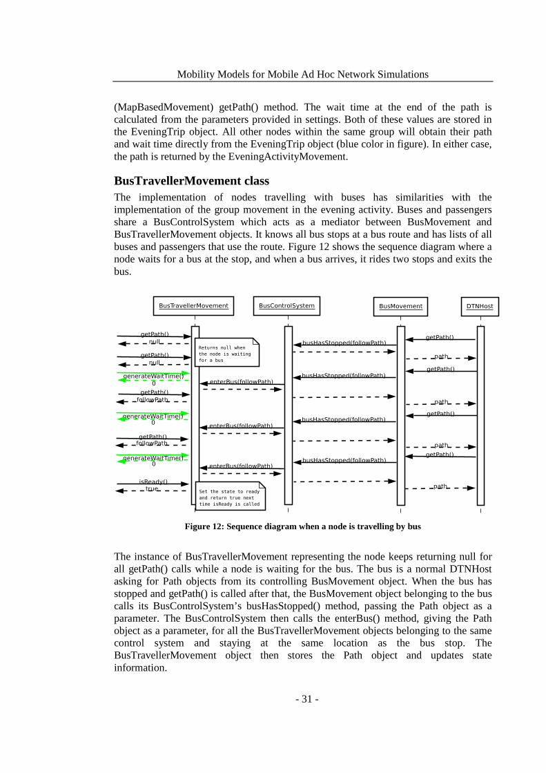
Mobility Models for Mobile Ad Hoc Network Simulations
- 31 -
(MapBasedMovement) getPath() method. The wait time at the end of the path is calculated from the parameters provided in settings. Both of these values are stored in the EveningTrip object. All other nodes within the same group will obtain their path and wait time directly from the EveningTrip object (blue color in figure). In either case, the path is returned by the EveningActivityMovement.
BusTravellerMovement class The implementation of nodes travelling with buses has similarities with the implementation of the group movement in the evening activity. Buses and passengers share a BusControlSystem which acts as a mediator between BusMovement and BusTravellerMovement objects. It knows all bus stops at a bus route and has lists of all buses and passengers that use the route. Figure 12 shows the sequence diagram where a node waits for a bus at the stop, and when a bus arrives, it rides two stops and exits the bus.
Figure 12: Sequence diagram when a node is travelling by bus
The instance of BusTravellerMovement representing the node keeps returning null for all getPath() calls while a node is waiting for the bus. The bus is a normal DTNHost asking for Path objects from its controlling BusMovement object. When the bus has stopped and getPath() is called after that, the BusMovement object belonging to the bus calls its BusControlSystem’s busHasStopped() method, passing the Path object as a parameter. The BusControlSystem then calls the enterBus() method, giving the Path object as a parameter, for all the BusTravellerMovement objects belonging to the same control system and staying at the same location as the bus stop. The BusTravellerMovement object then stores the Path object and updates state information.

Mobility Models for Mobile Ad Hoc Network Simulations
- 32 -
The next time getPath() is called for the BusTravellerMovement object, it will return the path it obtained from the BusControlSystem. The BusTravellerMovement object will use the path to be able to move exactly the same way as the bus, thereby appearing to travel on it. When the node has travelled the whole path, the generateWaitTime() method is called by the superclass (MovementModel), like usual. In BusTravellerMovement class, the method has been overridden to instead update state information so that the node is ready to accept a new Path object from the control system when the bus is ready to move again. The wait time returned by the BusTravellerMovement object is always zero. Note that while the bus stands still at the stop, the BusTravellerMovement returns null to all getPath() requestes, hence, it stands still like the bus. An interesting detail is that while the bus stands still, the system does not distinguish between nodes that are going to enter the bus and nodes already staying inside the bus. They all have the same state and are located at the exact same coordinates.
The BusTravellerMovement object continues to receive and use Path objects from the BusControlSystem until it reaches the end stop. The next time the BusControlSystem calls the BusTravellerMovement object’s enterBus() method, the BusTravellerMovement notices that it is at the end stop and switches the state to ready, so that when the isReady() method is called, the BusTravellerMovement can return true. Recall that the isReady() method is called between getPath() calls for all classes implementing the SwitchableMovement interface. For simplicity, only the last isReady() call is shown in the figure. When the BusTravellerMovement is ready, the following activity knows how to find to its destination from the bus stop.
CarMovement class The CarMovement class representing the car movement submodel inherits the MapBasedMovement model and implements the TransportMovement interface. It returns the shortest path between the current location and the destination when getPath() is called. Its isReady() method will return true after that.
4.3.3 BusMovement class The BusMovement is an extension of the MapRouteMovement class, which in turn is an extension of the MapBasedMovement class. The MapRouteMovement class is one of the classes included in the ONE’s default package. It moves a node according to a route defined in a WKT file in settings. The route is a list of checkpoints and the MapRouteMovement’s getPath() method always returns the shortest path from the current checkpoint to the next checkpoint. Dijkstra’s algorithm is used for calculation of shortest paths.
The MapRouteMovement class takes care of the movement according to a route. The BusMovement only needs to implement the communication with the BusControlSystem, i.e. inform the BusControlSystem that it has stopped. The BusMovement class communicates solely to the BusControlSystem class and is not aware of any passengers.

Mobility Models for Mobile Ad Hoc Network Simulations
- 33 -
4.4 Summary In this chapter we presented our movement model, the Working Day Movement model. We started from the requirements of the model and followed with the design of the model and explained how the requirements were met. We described each submodel and the use of the map in detail. Finally, we explained how the model was implemented into the ONE simulator.

Mobility Models for Mobile Ad Hoc Network Simulations
- 34 -
5 Experimental setup
This chapter describes the settings we used in our simulations and the measurements done. We begin by explaining the different metrics, after which we describe the default scenario.
5.1 Recorded Metrics For each simulation run, we measured 7 different mobility metrics. Additionally, we simulated the Epidemic routing protocol and used the performance metrics for sensitivity analysis. In the following subsections, we present details about each metric and in some cases more information about measurement practices and how the results should be interpreted.
5.1.1 Inter-contact times and contact durations We estimated the inter-contact and contact time distributions by sampling them from simulation runs of length T = 7 · 105s. Due to the finite simulation time, the longer events are less likely to get observed. This is because a larger fraction of them has the beginning or end outside the simulation time. This leads to a systematic error so that it is not easy to say whether there is an exponential decay in an empirical distribution or just this systematic error. To avoid this uncertainty, we adjust the experimental distributions as follows.
We assume that the events are uniformly distributed over a longer period of time. Then, consider the probability of an event of length x, p(x). Only events that begin during the time interval [0, T-x] will get recorded. To compensate this, the estimated probability density function p(x) is
),(')( xpxT
Txp
−=
where p'(x) denotes the measured density. We use p(x) for creating the Complementary Cumulative Density Functions (CCDF, P[X>x]). The same method was used also on the experimental data used as a reference. This decreases the effect caused by different length of the measurement period between different measurements.

Mobility Models for Mobile Ad Hoc Network Simulations
- 35 -
Inter-contact times or contact durations longer than the simulation time cannot be observed. This results in a cutoff in the tail of the distribution. The lost probability mass from the end of the tail is shifted to the other side, because the total probability density mass is always equal to 1. If t stands for the probability mass of the lost part of the tail, then the probability density function will be multiplied by 1/(1-t). This increase will cumulate in the CCDF leading to faster decline of the CCDF curve. In our experiments, a longer measurement period will lead to a smaller power-law exponent for the fist 12h of the distribution. This systematic error is not corrected by the aforementioned correction procedure. An option to correct this is to assume the longer inter-contact times follow the same distribution, calculate the lost probability mass in the tail and adjust the probability density function accordingly. However, we have already seen that the distribution of inter-contact times changes from a power-law to an exponential distribution after 12h and there is no guarantee that it stays exponential for even longer inter-contact times.
5.1.2 Unique encounters, total encounters and their comparison The unique encounters stand for the number of different other nodes a node has encountered during the simulation. By dividing the unique encounters with the total number of nodes, we get the fraction of the user population encountered by a node. We calculate a CCDF that shows the probability that this fraction for a randomly selected node is larger than or equal to x. This metric correlates with locality; Nodes moving within a small area will less likely meet many other nodes. From the distribution it is also possible to see differences among nodes; therefore, the previously defined CCDF also shows heterogeneity among nodes.
The total encounters stands for the number of times a node has encountered any other node. We calculate a CCDF that shows the probability that a randomly selected node has a number of total encounters greater than or equal to x. Since active nodes are more likely to encounter other nodes, this metric shows if there are different degrees of activity among nodes.
Finally, we plot a dot for each node on a scatter diagram where the x-axis stands for the total encounters and the y-axis stands for the unique encounters for each node. This illustrates differences between contact patterns among nodes. We are interested in differences between nodes in terms of the ratio of total- to unique encounters. Additionally, we are interested in differences between scenarios in terms of the ratio of the largest value to the smallest for both total- and unique encounters. We use a log-log scale to spot these differences in ratios. In other words, a specific distance and angle between two dots should always indicate the same proportional difference.
One can argue that with homogeneous movement, each node will encounter the same number of other nodes in total and a same size fraction of all the other nodes during a longer simulation. If nodes move according to different patterns and speeds within different sized areas, nodes will meet a different number of other nodes. Additionally, a node restricted to a small area will keep meeting the same nodes over and over, while a scout node exploring the simulation area will mostly meet new nodes. Therefore, the scatter diagram can be used to measure heterogeneity. Heterogeneous movement will

Mobility Models for Mobile Ad Hoc Network Simulations
- 36 -
result in dots all over the figure; while completely homogeneous movement will result in a group of dots all on the same spot.
5.1.3 Number of contacts between two contacts with a node The number of contacts during an inter-contact time metric is similar to the inter-contact times metric, except that instead of measuring the time until a node meets again, we count the number of other nodes both of the nodes meet separately. In contrast to the inter-contact times, the number of contacts during an inter-contact is not symmetric, i.e. during an inter-contact both nodes wait the exact same time but will meet a different number of nodes.
This metric has practical meaning. Some protocols make use of variables for message delivery likelihood. Each node has a variable for each other node corresponding to how good chance the node has to deliver a message to the other node. Some protocols, like MaxProp [27], adjust these variables based on contacts. The predictabilities are normalized in MaxProp; therefore, a contact with a specific node decreases all other predictabilities. It is necessary to have an understanding of how many contacts with other nodes happen between two contacts with the same node, when developing this kind of protocols. The value is different in different environments, and may additionally be distributed differently. Therefore, we want to see if different mobility characteristics have an impact on it and whether it can be controlled by some parameters in our movement model.
5.1.4 Hourly activity Song et al. [28] used the CRAWDAD trace [29] and counted for each hour of the day the total number of contacts between all users. The results were summed across all days of the trace period. They assumed that network traffic and usage of applications correlate with the contacts per hour, and therefore used the contacts to trigger sending of messages in their simulations. We think that the contacts per hour can be used as a metric itself for comparisons. We normalize the contacts counts so that they can be compared to contact counts from other scenarios.
We call the metric hourly activity. We measure hourly activity over a longer period of time and do not sum the contacts across all days, because not every model has the exact same day length or is periodic. We compare our hourly activity to the one from the CRAWDAD trace which we obtained by manually taking samples from a picture in [28].
5.1.5 Performance of the Epidemic routing protocol We measure latency, average hop count and packet delivery ratio for the Epidemic routing protocol to get an understanding of how different properties of our model affect routing protocols and how well packets can be delivered through the network. The metric correlates with the overall connectivity of the network and additionally serves as a metric for sensitivity analysis when experimenting with different parameters.
In our experiments, 0.7 messages are sent per node within a simulation time of 7 · 105s. This corresponds to 3–4 new messages sent each hour. The simulation time consists of a workweek plus additional warmup time for the buffer queues to stabilize as we will

Mobility Models for Mobile Ad Hoc Network Simulations
- 37 -
explain soon. The messages are uniformly distributed over this time interval and the senders and receivers are two randomly and independently selected nodes. Another idea would have been to concentrate the sending of messages to times where there is more activity, like Song et al. [28] did. This is necessary when we simulate a new protocol and want the conditions to be more realistic; however, we are simulating our mobility model and not a routing protocol. So we want to select such parameters that the results depends on as many mobility characteristics as possible but as few other aspects as possible. Triggering sends based on contacts would cause the number of sent packets to depend on the mobility model, which makes analysis of the results hard. Additionally we want to see the impact of nights when there is less activity.
The message sizes are uniformly distributed between 1 byte and 1MB and the transmission speed is 100KB/s. The time to live (TTL) parameter was set to one 24h and the buffer size large enough to never get full. The values were chosen to that nodes are not able to exchange all their messages during short contacts.
Like inter-contact times, contact durations and any events which durations are not significantly smaller than the simulation time, the longer events are less likely to get observed. This is true for messages as well, when we measure latencies, hop counts, etc. But in our experiments, we have a finite TTL; hence we can use a warmup period instead of an artificial correction procedure. This warmup period should not be confused with the one used for the mobility model to reach a steady state. This warmup period has two purposes. First of all, we want the network to be in a steady state in the sense of buffer queues in nodes and age of messages. Secondly, we want to allow recorded events to start during the warmup period so that longer packets get a fair treatment as well. We are not recording packets that were received during the warmup time and packets that are still being forwarded to the destination when the simulation ends. These together imply that a minimum warmup time of 2 · TTL is needed. One TTL is needed for the network to reach a steady state and one TTL is needed to make sure that none of the packets that were created during the unsteady state get recorded. Our TTL is 24h and we use a warmup period of 2 · 105s, which is roughly 2.3 · TTL.
There are two ways to measure packet delivery. The first one is to count the number of sent packets and the number of received packets during the real simulation time after the warmup. Statistically this will produce accurate results if the events are uniformly distributed over a longer period of time. The second approach is to track all the packets that were created during the real simulation time except during the last TTL of the simulation time, and then count the number of these packets that were received. The last TTL makes sure that every packet gets an equal opportunity to get delivered. We use the second approach, since we have a short simulation time and a periodic movement model. The first approach works if the time interval during which we track created and received packets is a multiple of the period. But we want to be able to compare the model to other models with different periods or no periods at all. For each scenario we run 5 simulations with different seed values for the random number generator and calculate the average with a 95% confidence interval.

Mobility Models for Mobile Ad Hoc Network Simulations
- 38 -
5.2 Scenario settings In this section we describe the settings and configurations used during the simulations. Whenever we refer to the default values or the default scenario, we mean the simulation scenario run with these settings. The default scenario was used for validation of the model, and the configuration file is presented in appendix A.
We used a map of the Helsinki center area with the surrounding districts. The size of the map was roughly 7000 × 8500m2. The area was divided into 4 main districts: A, B, C and D, see Figure 13. The districts are artificial and do not have any correlation to any real districts or areas within the Helsinki city. Additionally 3 districts were created to simulate movements between the center and other districts. Nodes belonging to these districts correspond to people working and living in different districts. Finally, we created one district to cover the whole simulation area. It has the same purpose as the 3 overlapping districts, except that the movement of the nodes in this large district is less local.
Figure 13: Map of Helsinki city with four artificia l districts used in the simulation
We used a population of 1000 nodes working in 200 offices and using 24 meeting spots for their evening activities. This numbers correspond to an average number of 5 employees per office and 40 persons per meeting spot. In practice, because of the overlapping districts, we will in some cases have two offices so close to each other that the nodes will meet so often during the workday that it seems as if the nodes are working in the same office. Table 1 shows the assignment of the nodes to the different districts.

Mobility Models for Mobile Ad Hoc Network Simulations
- 39 -
Table 1: The assignment of nodes, offices and meeting spots to the different districts
District Nodes Offices Meeting
spots A 150 30 4 B 50 10 1 C 100 20 2 D 100 20 2 E ( A and B) 100 20 2 F (A and C) 150 30 4 G (A and D) 150 30 4 H (Whole map) 200 40 5
Each district was assigned one bus route. Districts A–G were assigned 2 busses each, and district H was assigned 4 busses. Since the H districts is so large compared to the other districts, it makes sense to have more buses so that the waiting times would not be unnecessary long.
Figure 14: Bus routes used in the simulations. The left figure shows the bus routes for districts A–D, while the right figure shows for E–H (yellow route is for H).
Half of all the nodes were set to travel by car instead of bus. The speed of the cars was set to 20m/s to make it a clearly faster way to move between locations. The walking speed for nodes was set to 0.8–1.4m/s, which is also used for all indoor movement. Buses were moving with speed 7–10m/s with a 10–30s waiting at each stop. The probability to do some evening activity after work was set to 0.5 with the group sizes uniformly distributed between 1 and 3.
A working day length of 28800s was chosen. It corresponds to 8 hours and is a typical length of a work day in most professions. The pause times inside the office were drawn from a Pareto distribution with coefficient 0.5 and minimum value 10s. The office size was set to a 100m × 100m square. The size of the office was chosen so that it would compensate for the lack of floors, walls, etc. A real office has rooms and corridors, hence, geographically close nodes are not necessarily in contact. The differences in

Mobility Models for Mobile Ad Hoc Network Simulations
- 40 -
schedules of nodes were drawn from a normal distribution with a standard deviation of 7200s. This corresponds to a situation where 68% of the population goes to work between 7 and 11 in the morning. For the background movement, corresponding to taxies, delivery of goods, etc, we had 10 nodes. These were moving according to the SPMBM described earlier.
The transmit range of all nodes was set to 10m, which is common for Bluetooth devices. Since we have not modeled walls or other obstacles, the nodes were considered to be in contact when they were closer to each other than the transmit range. In the real world, there is usually a connection setup delay and the frequency of scanning for other devices is usually limited to keep energy consumption low, leading to detection delay. It is worth to note that this phenomenon has probably affected real world contact traces used for comparison. A study about optimal probing of contacts can be found in [30].
We used a warmup period of half a day for the movement model, which is sufficient due to the periodic nature of the movement model. For comparison, we simulated a RWP scenario on a same sized simulation area with 1000 nodes, moving with speed 0.5–5m/s and pause time 1–3600s, both uniformly distributed. When we refer to RWP in the comparisons, we refer to this scenario.

Mobility Models for Mobile Ad Hoc Network Simulations
- 41 -
6 Results
We validated our movement model by comparing it to data from real world measurement experiments. We used the inter-contact times, contact durations and hourly activity as metrics, since data from real user traces is available for these metrics. Additionally, we explore the impact of different parameters and determine how customizable the model is.
6.1 Validation of the model We ran the simulation with the default settings described in the previous chapter, and measured inter-contact times, contact durations, hourly activity and total encounters vs. unique encounters for each node.
Figure 15 shows the inter-contact time distribution of our model compared to RWP and the iMote trace. In both our model and the iMote trace, we have a power-law distribution up to roughly half a day (~43200s), after which an exponential decay follows.
102
103
104
105
10−2
10−1
100
P[X
>x]
Time [s]
iMotesDefaultRWP
Figure 15: Inter-contact times of Working Day Movement compared to RWP and iMote trace

Mobility Models for Mobile Ad Hoc Network Simulations
- 42 -
Our model has not been configured to produce a power-law with the exact same exponent as the one in the iMote traces, since the coefficient can vary between environments. Power-law exponents were calculated for different traces in [10], and the exponents ranged from 0.4 to 0.9 when no correction procedures had been applied to the results. In our model, it is possible to vary the power-law exponent by altering different parameters to better match a specific environment.
Figure 16 shows that the contact durations follow a similar curve as the iMote trace. However, it is worth to note that many simple models can be configured to produce almost any kind of distribution of contact durations. The easiest way is to just configure pause times to follow such a distribution that the resulting distribution of the time two nodes pause near each other follows the desired distribution.
100
101
102
103
104
105
10−4
10−3
10−2
10−1
100
P[X
>x]
Time [s]
iMotesDefaultRWP
Figure 16: Contact durations of the Working Day Movement model compared to the RWP model and the iMote trace
In Figure 17, we have plotted the hourly activity from a three day period of time. The Dartmouth trace is shown for comparison. We can see that there are two peeks during each day in our model like in the Dartmouth trace. The Dartmouth trace is from a campus area, therefore the movement can be different than in the center of a city. Hence, as a metric for validation of a model, we can only say that our model is heterogeneous in time like the Dartmouth trace. Configuring our model to produce peaks at the exact same locations as the Dartmouth trace is not necessarily any more realistic, instead just more specific to the Dartmouth environment. In addition, it is worth to note that the contacts in the Dartmouth trace were derived from access point data and may only constitute a portion of all contacts.

Mobility Models for Mobile Ad Hoc Network Simulations
- 43 -
30 40 50 60 70 80 900
0.1
0.2
0.3
0.4
0.5
0.6
0.7
0.8
0.9
1
Time [h]
Hou
rly a
ctiv
ity
DartmouthDefaultRWP
Figure 17: Hourly activity of the Working Day Movement model compared to RWP and Dartmouth trace
Figure 18 shows a scatter diagram where the total- vs. unique encounters have been plotted for each node in our model. The result is compared to the RWP model, and it is possible to see that there are clear differences between nodes in our model and the unique encounters are not proportional to the total encounters.
In section 5.1.2 we stated that realistic user movement is heterogeneous and that the scatter diagram with each node’s total- and unique encounters is one way to measure heterogeneity. We do not have any good data to compare our scatter diagram to. In [26] they plotted a similar diagram but on a linear scale for the USC trace. Since nodes were often switched off in the trace, their diagram cannot directly be compared to our diagram. If the length of the total time during which a device is switched on is uniformly distributed between nodes, the result is that more of the dots will be closer to the origin. In this case, the RWP results in a thin line from the origin to the last spot which is a node having the longest on-time. A curve instead of a line is a sign of a long simulation time and bounded simulation area. Nodes that have been switched on for a longer time have already met most of the other nodes and are less likely to encounter new nodes. The total encounter count will increase while the unique encounter count will not as fast as in the beginning. Hence, with on/off times modeled, a line or curve is not a sign of heterogeneity. The USC trace was not a line or curve, and it is possible to see that the unique encounters are not directly proportional to the total encounters, like with our model.

Mobility Models for Mobile Ad Hoc Network Simulations
- 44 -
101
102
103
104
101
102
103
Uni
que
enco
unte
rs
Total encounters10
110
210
310
410
1
102
103
Uni
que
enco
unte
rs
Total encounters Figure 18: Total encounters vs. unique encounters for each node plotted on a scatter diagram for both the Working Day Movement model and RWP
6.2 Exploring the parameter space To investigate and to get a better understanding of the impact of different parameters of the model, we simulated scenarios where each parameter was set to extreme values. It is essential to have an understanding of the sensitivity of the parameters in order to model a specific environment. Finally, we want to spot parameters and properties that do not have an impact and can be removed from the model in future versions. Dependencies between parameters have not been considered in most scenarios.
6.2.1 Density of nodes First of all, we want to find out the impact of the density of nodes. In this experiment we only consider the number of nodes moving according to the WDM model and not bus nodes or SPMBM nodes. Neither do we change the number of offices, meeting spots, etc. Another option would have been to adjust the number of offices and meeting spots to keep the nodes per office and nodes per meeting spot ratio intact.
We simulated 4 scenarios with different amounts of nodes; 100 nodes, 500 nodes, 1000 nodes and 2000 nodes. For ease of configuration, we simulated the scenarios without any districts. The scenario with 100 nodes was not included in the graphs because the error ratio was too high. Simulations with more nodes produce more events; therefore the results are more reliable as well. Furthermore, the systematic errors from groups having to wait too long to be full and other defects became too big in the scenario with 100 nodes.
The impact of the density did not become fully clear after these experiments. Figure 19 shows the inter-contact times distribution of the three scenarios.

Mobility Models for Mobile Ad Hoc Network Simulations
- 45 -
102
103
104
105
10−2
10−1
100
P[X
>x]
Time [s]
iMotes1000 nodes (No Districts)500 nodes2000 nodes
Figure 19: Inter-contact times with different node densities
The small drop around 2000s is a result from the bus route. The map used when districts are disabled only has one cyclic bus route, covering the whole area. Since it takes about 2000s for a bus to drive one round, it will keep encountering with nodes having their desk or home within radio reach of the bus route. This will result in many inter-contact times of length 2000s. With fewer nodes, this drop becomes more significant. This is because the number of offices and meeting spots are constant, which results in a situation with fewer nodes per office and meeting spot, which in turn generates fewer events. The events resulting from buses grow linearly in response to the number of nodes, while the events from offices grow by the number of nodes squared.
The motivation behind this assumption is that one node has a certain probability to have its home or office located at the bus route. If one node will generate x inter-contacts with a certain number of busses, then n nodes will generate nx inter-contacts with the same buses. While in an office, if 2 nodes result in x inter-contacts, then n nodes can result in n(n-1)/2 inter-contacts. The inter-contact times from the buses are all approximately of the same length, while other contacts from offices are not. Thus, we have a small drop or step in the curve.
Even though one would expect that the density of nodes has a huge impact, it does not become clear from our results. The number of encounters with other nodes for each node is almost twice as high when the number of nodes is doubled. Other than that, only the routing protocol simulations revealed a difference.
Figure 20 shows the results from the epidemic routing protocol simulation. The performance does not seem to change drastically when the number of nodes increases. At first one would also assume that the performance increases when there are more nodes. This is true, but in our case also more messages are sent. More nodes result in

Mobility Models for Mobile Ad Hoc Network Simulations
- 46 -
more potential routes for packets to travel. While this improves the performance, the bandwidth still sets a limit at some point since a packet cannot be copied to an infinite number of nodes within a short contact, so all potential routes are not valid. Additionally, in our scenarios, more nodes imply more packets to be transferred during a contact.
Figure 20: Performance of the Epidemic routing protocol with different node densities
6.2.2 Use of buses or cars The purpose of this experiment is to find out if it makes any difference whether nodes travel by car or by bus. We simulate one scenario where all the nodes travel by bus and another one where all of them travel by car. Bus nodes were left running empty on their routes in the scenario where all nodes travelled by car. In these experiments we used the default scenario with districts.
Figure 21 shows the inter-contact time distribution for all three scenarios compared to the iMote trace. An interesting observation is the difference in the power-law exponent, which is generally considered to characterize the feasibility of routing.
102
103
104
105
10−2
10−1
100
P[X
>x]
Time [s]
iMotes50% use car (Default)0% use car100% use car
Figure 21: Inter-contact times when nodes travel by car, by bus and 50/50 car/bus
Latency
0
10000
20000
30000
40000
50000
Density 500 Default-nodistricts
Density 2000
HopCount
0
2
4
6
8
10
12
Density 500 Default-no districts Density 2000
Delivery ratio
0.0%
20.0%
40.0%
60.0%
80.0%
100.0%
Density 500 Default-nodistricts
Density 2000

Mobility Models for Mobile Ad Hoc Network Simulations
- 47 -
In the scenario with no buses, nodes move quicker and have fewer chances to encounter other nodes on their way home or to work. Therefore, most of the contacts are contacts with colleagues from the same office, neighbors and other people that the nodes meet between shorter time intervals than half a day. Hence, there are more short inter-contact times than long ones. On the other hand, buses make sure that people doing activities geographically near each other have good chances to meet on the bus stop if they do not have huge differences between their schedules. Finally, people can meet in the bus if they do not live in completely different districts. Figure 22 shows that when all the nodes use buses, they meet roughly twice as large a fraction of all the other nodes compared to when they travel by car.
0 10 20 30 40 50 60 70 80 90 1000
0.1
0.2
0.3
0.4
0.5
0.6
0.7
0.8
0.9
1
P[X
>x]
Fraction of user population [%]
50% use car (Default)0% use car100% use car
Figure 22: Fraction of user population encountered when all nodes travel by car, all travel by bus and 50/50 car/bus
The result of the meeting opportunities at bus stops and in the bus is that many node pairs meet between longer time intervals, for example: once a day on their way to work or sometimes on the bus stop on their way home from the evening activity. In this case there are more long inter-contact times. The huge number of contact events happening at bus stops or inside the bus is also visible in the hourly activity graph, see Figure 23. We have two clear peeks resulting from nodes travelling by bus to and from work. The travelling to the meeting spot for evening activity does not result in a peek for two reasons. First, only half of the nodes do evening activity. Second, different groups of nodes end their evening activity at different times; therefore, there will be less clustering nodes at the bus stops. Remember that n nodes meeting at a bus stop results in n(n-1)/2 contacts.

Mobility Models for Mobile Ad Hoc Network Simulations
- 48 -
30 40 50 60 70 80 900
0.1
0.2
0.3
0.4
0.5
0.6
0.7
0.8
0.9
1
Time [h]
Hou
rly a
ctiv
ity
Dartmouth50% use car (Default)0% use car100% use car
Figure 23: Hourly activity when all nodes travel by car, all travel by bus and 50/50 car/bus
We observed that even though the bus movement is more complex and nodes meet different number of people in the bus depending on the route they need to travel, still, it is not more heterogeneous if measured on the scatter diagram (see Figure 24). Instead it seems as if the car movement is more heterogeneous.
One reason for this is that the bus routes are circular and at each stop there enters a certain group of nodes in the bus and a certain group leaves the bus. Some small differences are caused by randomness, especially by the evening activity. Still, some nodes travel longer routes in general than others, which results in some nodes encountering more nodes. If a node encounters n nodes each day in the bus, the result is about n unique encounters and tn total encounters resulting from the bus trips after t days. Both are proportional to n, which explains the nature of the figure where the dots are in a thin oval area.
101
102
103
104
101
102
103
Uni
que
enco
unte
rs
Total encounters10
110
210
310
410
1
102
103
Uni
que
enco
unte
rs
Total encounters10
110
210
310
410
1
102
103
Uni
que
enco
unte
rs
Total encounters Figure 24: Unique- vs. total encounters when nodes travel only by bus (left), 50/50 car/bus (middle) and only by car (right)

Mobility Models for Mobile Ad Hoc Network Simulations
- 49 -
The car movement on the other hand generates fewer encounters, thereby not affecting the outcome so much itself. Thereby the heterogeneity is affected more by the other activities.
Figure 25 shows how the epidemic routing protocol performed under both conditions compared to the default scenario. The impact of the transport movement on the performance is remarkable. Bus stops and buses are excellent places to exchange packets between nodes. There is plenty of time to transfer large messages and nodes which otherwise do not have anything in common meet. Cars on the other hand move fast and no large messages can be exchanged. In most cases they will only encounter a few other nodes on their way.
Figure 25: Performance of the Epidemic routing protocol when all nodes travel by car, all travel by bus and 50/50 car/bus
The conclusion is that the way nodes move between activities has a significant impact on mobility and how routing protocols will perform. Therefore, much effort should be put on modeling movement between activities correctly.
6.2.3 Use of districts We ran a simulation where no districts were used, i.e. with one group of nodes having their homes, offices and meeting spots uniformly distributed over the whole map. All nodes in the group not owning a car used a bus route covering the whole map (yellow route in Figure 14). The bus route starts from district B and ends in C.
The inter-contact times were not affected by districts, but the contact durations were slightly affected. Figure 26 shows that there are more 20–10000s long contacts in the scenario without districts. This is a result of the long bus route. A long bus route leads to more people travelling together a longer time in the bus, which implies more long contact durations. Additionally, when homes, offices and meeting spots are uniformly distributed over the map, nodes have to travel longer distances; therefore, it is less likely that nodes choose to walk between activities. Within a small district, the distances between a node’s office, home and meeting spot are likely to be shorter. Hence, more nodes will choose to walk instead of using a bus.
Latency
0
10000
20000
30000
40000
50000
60000
No cars Default Only Cars
HopCount
0123456789
No cars Default Only Cars
Delivery ratio
0.0%
20.0%
40.0%
60.0%
80.0%
100.0%
No cars Default Only Cars

Mobility Models for Mobile Ad Hoc Network Simulations
- 50 -
100
101
102
103
104
105
10−4
10−3
10−2
10−1
100
P[X
>x]
Time [s]
iMotesDefaultNo districts
Figure 26: Contact durations when districts are used and not used
Figure 27 shows the CCDF of the fraction of user population encountered by a node. As expected, the use of districts reduced significantly the fraction of user population encountered by nodes, and therefore is a good mechanism to control locality of node movement.
0 10 20 30 40 50 60 70 80 90 1000
0.1
0.2
0.3
0.4
0.5
0.6
0.7
0.8
0.9
1
P[X
>x]
Fraction of user population [%]
DefaultNo districts
Figure 27: Fraction of user population encountered when districts are used and not used

Mobility Models for Mobile Ad Hoc Network Simulations
- 51 -
Figure 28 shows the total- vs. unique encounters plotted on a scatter diagram. An interesting observation is that districts seem to introduce more heterogeneity among nodes. Different sized districts with different node densities and different bus routes are likely to result in a variety of different proportions between unique and total encounters.
101
102
103
104
105
101
102
103
Uni
que
enco
unte
rs
Total encounters10
110
210
310
410
510
1
102
103
Uni
que
enco
unte
rsTotal encounters
Figure 28: Total- vs. unique encounters when districts are used (left) and not used (right)
The use of districts has a clear impact on the routing. Figure 29 shows the results of the epidemic routing protocol. The protocol performed better when there were no districts restricting node movement.
Figure 29: Performance of the Epidemic routing protocol when districts are used and not used
6.2.4 Use of a specific map With the following experiment, we wanted to determine the impact of the road net. We simulate a scenario where we have the exact same number of nodes moving on a Manhattan like map of the same size as the Helsinki map. One block on the Manhattan map is a square with the side 180m. The same number of homes, offices and meeting spots were used in the Manhattan scenario. To minimize the differences in other characteristics we did not use any districts and let all the homes, offices and meeting spots be uniformly distributed over the map. Hence, we compared the results to the default scenario without districts.
Latency
0
10000
20000
30000
40000
50000
No districts Default
HopCount
0123456789
No districts Default
Delivery ratio
0.0%
20.0%
40.0%
60.0%
80.0%
100.0%
No districts Default

Mobility Models for Mobile Ad Hoc Network Simulations
- 52 -
A different map did not have an impact on the inter-contact times. Figure 30 shows that the contact durations were slightly affected in the sense that there were less 10–10000s long contacts in the Manhattan scenario. These are likely to originate from nodes travelling inside buses and waiting at bus stops. The bus routes were different. The Manhattan map had a circular bus route, while the Helsinki map had a long route starting from district B, going through A and D, and finally ending in C. A longer bus route, which is not circular, results in a situation where several nodes enter the bus when it goes in the wrong direction, thereby taking an extra ride to one end of the bus route before reaching the final destination. In this case, buses will be more crowded and there will be more long contacts.
100
101
102
103
104
105
10−4
10−3
10−2
10−1
100
P[X
>x]
Time [s]
iMotesNo DistrictsManhattan
Figure 30: Contact durations on different maps
Figure 31 illustrates that in the Helsinki scenario, the nodes moving by bus encountered both a larger fraction of all other nodes and more nodes in total. The graphs show that roughly around 50% of the nodes, which is the percentage of nodes moving by bus, have more encounters. This is due to the fact that in the Helsinki scenario, any node can potentially meet any other node inside the bus, and after a simulation with infinite time, all nodes moving by bus have eventually met each other. On the contrary, this is not the case for the Manhattan scenario, due to the circular bus route.

Mobility Models for Mobile Ad Hoc Network Simulations
- 53 -
0 0.5 1 1.5 2 2.5 3 3.5
x 104
0
0.1
0.2
0.3
0.4
0.5
0.6
0.7
0.8
0.9
1
P[X
>x]
Total encounters
No DistrictsManhattan
0 10 20 30 40 50 60 70 80 90 1000
0.1
0.2
0.3
0.4
0.5
0.6
0.7
0.8
0.9
1
P[X
>x]
Fraction of user population [%]
No DistrictsManhattan
Figure 31: Total encounters (left) and the fraction of user population encountered by nodes (right) on different maps
It seems as if the small differences are all a result of the bus routes. The details of the road net itself have a minimal impact. However, major discontinuities in the road net coming from obstacles such as sea and mountains, do have an impact on bus routes. The road net can have a dramatic impact in more extreme scenarios. An extreme scenario would be when the road net is completely discontinuous due to islands, in which case some nodes are never able to communicate with others.
For sensitivity analysis, Figure 32 shows the results from the simulation of the epidemic routing protocol. When taking into account the error margins, we cannot say that the map has an impact.
Figure 32: Performance of the Epidemic routing protocol on different maps
6.2.5 Number of offices The parameter controlling the number of offices has an impact on two things; the node density within an office and the clustering of nodes during the work time. The situation where many nodes meet at an office introduces a good opportunity for a node to distribute its packets to all other nodes at the same office which will all carry the packets to different places after work. On the other hand, nodes are less likely to meet nodes from other offices since the offices will be sparsely located on the map.
A scenario with many offices with few nodes each can in theory cover the map in such a way that offices are partially overlapping and all offices are connected to each other. In this case messages can better be routed during the work day, but an individual office will not be such a good central distribution point as in a scenario with fewer offices.
Latency
05000
1000015000200002500030000350004000045000
Manhattan Default-no districts
HopCount
0123456789
Manhattan Default-no districts
Delivery ratio
0.0%
20.0%
40.0%
60.0%
80.0%
100.0%
Manhattan Default-no districts

Mobility Models for Mobile Ad Hoc Network Simulations
- 54 -
To get a better understanding of the parameter we simulated two scenarios with different numbers of offices; one with 50 offices (20 nodes per office in average) and one with 1000 offices (one node per office in average). To make the experiment less dependent on the positioning of offices, we did not use districts and the offices were uniformly distributed over the map.
Figure 33 shows the inter-contact time distribution of both the scenarios compared to the default scenario without districts. There are more short inter-contact times in the scenario with 50 offices. This is because the inter-contact times within an office are most often short due to the nature of the Pareto distribution of the wait times. A node will quickly move away from its desk and return and meet its nearby nodes again, resulting in short inter-contact times. Finally, when there are more nodes inside an office, there are more possible node pairs, which leads to more inter-contact times.
102
103
104
105
10−2
10−1
100
P[X
>x]
Time [s]
iMotes200 offices (No Districts)50 offices1000 offices
Figure 33: Inter-contact times with different number of offices
Figure 34 shows the performance of the Epidemic routing protocol. Fewer offices directly imply more nodes at an office. It seems as this type of meetings are greatly improving the connectivity of the network.
Figure 34: Performance of the Epidemic routing protocol with different numbers of offices
Latency
0
10000
20000
30000
40000
50000
50 off ices Default-nodistricts
1000 off ices
HopCount
0
2
4
6
8
10
50 off ices Default-no districts 1000 of f ices
Delivery ratio
0.0%
20.0%
40.0%
60.0%
80.0%
100.0%
50 off ices Default-nodistricts
1000 off ices

Mobility Models for Mobile Ad Hoc Network Simulations
- 55 -
6.2.6 Office Size We studied how the office size affects our metrics, by simulating two scenarios. In the first scenario we used 10m×10m office spaces and in the other 500m×500m office spaces. Figure 35 shows the inter-contact time distribution compared to the default scenario with 100m×100m offices.
The power-law exponent has an interesting tendency to be smaller both for the small and the large office compared to the default size office. It appears to be so that the exponent decreases when nodes within the office are more often in contact with other nodes passing by at nearby roads. In the scenario with an office size of 10m×10m, all nodes inside offices were in contact with other nodes passing by, while in the scenario with 500m × 500m offices, many streets were inside the bounds of the office, thereby resulting in many contacts.
102
103
104
105
10−2
10−1
100
P[X
>x]
Time [s]
iMotesOffice size 100 (Default)Office size 10Office size 500
Figure 35: Inter-contact times with different office sizes
The impact of the office size on the inter-contact times was additionally studied with five additional scenarios with different office sizes (side lengths: 10m, 50m, 150m, 200m and 300m) on the Manhattan map. The block size was 180m × 180m in all scenarios. The Manhattan map was selected because each block on the map is the same size. Figure 36 shows the inter-contact times distribution. The power-law exponent is indeed similar with a large and a small office size.

Mobility Models for Mobile Ad Hoc Network Simulations
- 56 -
102
103
104
105
10−0.7
10−0.6
10−0.5
10−0.4
10−0.3
10−0.2
10−0.1
100
P[X
>x]
Time [s]
iMotes10m50m150m200m300m
Figure 36: Inter-contact times of additional office size experiments on the Manhattan map
Figure 37 shows the distribution of contact durations. In the scenario with small offices, nodes within an office were most of the time in contact with each other; therefore, we have so many long contact durations.
100
101
102
103
104
105
10−4
10−3
10−2
10−1
100
P[X
>x]
Time [s]
iMotesOffice size 100 (Default)Office size 10Office size 500
Figure 37: Contact durations with different office sizes
Figure 38 shows that only the scenario with office sizes of a square with the side 10m differs from the other two when the performance of the Epidemic routing protocol is compared. The performance gain is a result from nodes inside the office being so close to the road; therefore they meet all other nodes passing by.

Mobility Models for Mobile Ad Hoc Network Simulations
- 57 -
Figure 38: Performance of the Epidemic routing protocol with different office sizes
Even if our previous experiments do not show that the geometry of the map has an impact, this experiment shows that the block size in conjunction with the office size has. This experiment shows the shortcomings of a 2d model where no attenuation of walls is modeled.
6.2.7 Wait times inside office The office activity submodel is a first level abstraction of movement inside offices in general. In the real world there are several different buildings and the movement inside them may differ a lot between them. We experiment with different pause times, since our model has a parameter to control the pausing.
We conducted two experiments with different pause times. In the fist one, nodes were not pausing at all, resulting in continuous movement. In the second scenario, the pause time was set to infinite, thereby forcing nodes to sit still on their desk the whole workday.
The most important observation of this experiment is the impact of the pause time on the inter-contact time distribution. Figure 39 shows how the power-law exponent of the inter-contact time distribution changes. The curve of the scenario with no wait times clearly goes below the curve of the iMote trace. The continuous movement leads to nodes meeting each other between shorter time intervals, leading to more short inter-contact times. This shifts a portion of the probability density mass to the left.
Latency
0
10000
20000
30000
40000
50000
Office Size 10 Default Off ice Size 500
HopCount
0
2
4
6
8
10
Off ice Size 10 Default Off ice Size 500
Delivery ratio
0.0%
20.0%
40.0%
60.0%
80.0%
100.0%
Office Size 10 Default Off ice Size 500

Mobility Models for Mobile Ad Hoc Network Simulations
- 58 -
102
103
104
105
10−2
10−1
100
P[X
>x]
Time [s]
iMotesPareto (Default)No waitingNo moving
Figure 39: Inter-contact times with different pause times inside offices
Figure 40 illustrates that the distribution of contact durations was also affected. Obviously, when nodes are pausing less, there will be more contacts in total and the contacts will be shorter.
100
101
102
103
104
105
10−4
10−3
10−2
10−1
100
P[X
>x]
Time [s]
iMotesPareto (Default)No waitingNo moving
Figure 40: Contact durations with different pause times inside offices
Another interesting observation is the impact on the distribution of the number of contacts between two contacts with the same node, shown in Figure 41. The pause time parameter seems to be the only one able to make a relevant change in this metric, i.e. a change in the nature of the distribution. Of course, any parameter or feature resulting in

Mobility Models for Mobile Ad Hoc Network Simulations
- 59 -
more contacts in general, like the density of nodes parameter, will have an impact, but the nature of the distribution in all other cases is still exponential. However, by changing the pause time parameter, we were able to get a power-law tendency up to roughly 1000 contacts. When working with protocols such as MaxProp, scenarios with different values for this parameter can be useful.
100
101
102
103
104
105
10−4
10−3
10−2
10−1
100
P[X
>x]
Contacts
Pareto (Default)No waitingNo moving
Figure 41: Number of contacts during an inter-contact time for different pause times inside offices
The hourly activity diagram is shown in Figure 42. It is possible to see that most of the contacts originate from the office movement submodel. Due to normalization of the results, the contacts from the evening activity or buses get drowned in the huge amount of contacts from the fast office movement.

Mobility Models for Mobile Ad Hoc Network Simulations
- 60 -
30 40 50 60 70 80 900
0.1
0.2
0.3
0.4
0.5
0.6
0.7
0.8
0.9
1
Time [h]
Hou
rly a
ctiv
ity
DartmouthPareto (Default)No waitingNo moving
Figure 42: Hourly activity for different pause times inside offices
Figure 43 compares the two extreme scenarios and the default scenario in terms of total- vs. unique encounters. The figure shows more heterogeneity for the scenario with no pausing inside the office. This is due to the fact that the office movement dominates in the generation of encounters. The nature of the office movement is such that it generates few unique encounters, at most the number of nodes within the building and some occasional nodes passing near the office. Therefore each node gets its unique encounters from other activities.
The more nodes there are within the same office or area where several offices are co-located, the more total encounters there will be. Some nodes will work in offices with few nodes while others in offices with more nodes. Additionally there is a chance that office spaces are overlapping. The more nodes within the same office or area of co-located offices, the more total encounters will the nodes have. Hence, more movement implies more scattering in the total encounters direction.
101
102
103
104
101
102
103
Uni
que
enco
unte
rs
Total encounters10
110
210
310
410
1
102
103
Uni
que
enco
unte
rs
Total encounters10
110
210
310
410
1
102
103
Uni
que
enco
unte
rs
Total encounters Figure 43: Total- vs. unique encounters for different pause times inside offices. No waiting (left), default (middle) and infinite wait (right)
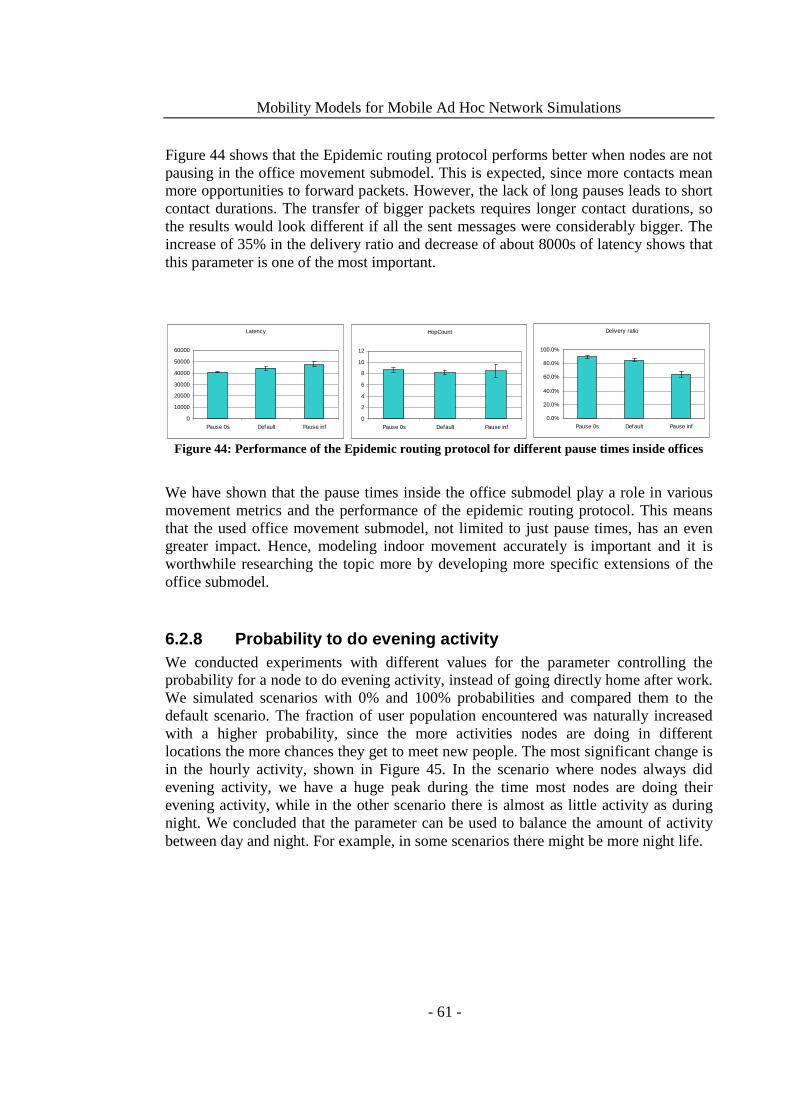
Mobility Models for Mobile Ad Hoc Network Simulations
- 61 -
Figure 44 shows that the Epidemic routing protocol performs better when nodes are not pausing in the office movement submodel. This is expected, since more contacts mean more opportunities to forward packets. However, the lack of long pauses leads to short contact durations. The transfer of bigger packets requires longer contact durations, so the results would look different if all the sent messages were considerably bigger. The increase of 35% in the delivery ratio and decrease of about 8000s of latency shows that this parameter is one of the most important.
Figure 44: Performance of the Epidemic routing protocol for different pause times inside offices
We have shown that the pause times inside the office submodel play a role in various movement metrics and the performance of the epidemic routing protocol. This means that the used office movement submodel, not limited to just pause times, has an even greater impact. Hence, modeling indoor movement accurately is important and it is worthwhile researching the topic more by developing more specific extensions of the office submodel.
6.2.8 Probability to do evening activity We conducted experiments with different values for the parameter controlling the probability for a node to do evening activity, instead of going directly home after work. We simulated scenarios with 0% and 100% probabilities and compared them to the default scenario. The fraction of user population encountered was naturally increased with a higher probability, since the more activities nodes are doing in different locations the more chances they get to meet new people. The most significant change is in the hourly activity, shown in Figure 45. In the scenario where nodes always did evening activity, we have a huge peak during the time most nodes are doing their evening activity, while in the other scenario there is almost as little activity as during night. We concluded that the parameter can be used to balance the amount of activity between day and night. For example, in some scenarios there might be more night life.
Latency
0
10000
20000
30000
40000
50000
60000
Pause 0s Default Pause inf
HopCount
0
2
4
6
8
10
12
Pause 0s Default Pause inf
Delivery ratio
0.0%
20.0%
40.0%
60.0%
80.0%
100.0%
Pause 0s Default Pause inf

Mobility Models for Mobile Ad Hoc Network Simulations
- 62 -
30 40 50 60 70 80 900
0.1
0.2
0.3
0.4
0.5
0.6
0.7
0.8
0.9
1
Time [h]
Hou
rly a
ctiv
ity
Dartmouth50% do evening activity (Default)0% do evening activity100% do evening activity
Figure 45: Hourly activity for different probabilit ies to do evening activity
Figure 46 shows that the evening activity decreases the heterogeneity. The reason for this phenomenon is that the evening activity is the same for all nodes. The only difference between nodes is the meeting spot. Group size and the decision to do the activity are randomly drawn in an equal way for each node every time. The evening activity movement follows the MBM model which is a homogeneous movement model.
101
102
103
104
101
102
103
Uni
que
enco
unte
rs
Total encounters10
110
210
310
410
1
102
103
Uni
que
enco
unte
rs
Total encounters10
110
210
310
410
1
102
103
Uni
que
enco
unte
rs
Total encounters Figure 46: Total- vs. unique encounter for No evening activity (left), 50% (middle) and 100% (right)
The performance of the Epidemic routing protocol is sensitive to the parameter controlling the probability to do evening activity, see Figure 47. This does not necessarily mean that the details of the evening activity itself constitute the performance gain in the epidemic routing protocol experiment. It is likely that the cause of this phenomenon is the decrease in locality; a node moves between three activities instead of two. The remarkable impact on the routing results shows not only the importance of the parameter, but the importance of modeling right activities. In the real world, many people do various activities in different locations during the day. Some

Mobility Models for Mobile Ad Hoc Network Simulations
- 63 -
have jobs requiring movement between offices, while others are part time employees at some company while still attending some lectures in a university. Hence, this experiment shows the importance of modeling the right activities.
Figure 47: Performance of the Epidemic routing protocol for different evening activity probabilities
6.2.9 Evening activity group size We also experimented with different evening activity group sizes. In the first scenario we did not have any group movement. This was achieved by configuring the group size to one. In the second scenario, the group sizes were uniformly distributed between 1 and 10.
The inter-contact times distribution was not affected, but on the other hand we got more long contact durations, see Figure 48. In many cases it may take a long time for all nodes in a large group to be present at the meeting spot. Therefore, we will have unrealistically many long contact durations. In a simulation with many nodes in proportion to meeting spots, this will not be significant.
100
101
102
103
104
105
10−4
10−3
10−2
10−1
100
P[X
>x]
Time [s]
iMotes1−3 nodes/group (Default)No groups1−10 nodes/group
Figure 48: Contact durations
Latency
0
10000
20000
30000
40000
50000
60000
Evening activity0%
Default Evening activity100%
HopCount
0
2
4
6
8
10
Evening activity 0% Default Evening activity100%
Delivery ratio
0.0%
20.0%
40.0%
60.0%
80.0%
100.0%
Evening activity0%
Default Evening activity100%

Mobility Models for Mobile Ad Hoc Network Simulations
- 64 -
The group size does not seem to have a clear impact on any other measurements. Figure 49 shows that the routing results were similar in all three scenarios. The scenario with group sizes between 1 and 10 differs a bit from the other two, but not significantly. We believe that the difference is mostly due to the tendency of big groups not getting full as fast. However, the small impact of this parameter raises the question whether the parameter is needed at all. Moreover, there is probably not a need to have additional group movement, when buses already cover group movement.
Figure 49: Performance of the Epidemic routing protocol for different group sizes
6.2.10 Evening activity pause time The impact of the length of the pause times for the evening activity was also explored. It was set to 0s in the first scenario and 2–4h in the second one. No significant changes were observed. However, Figure 50 shows that there is a small improvement in the performance of the epidemic routing protocol when the pause times are longer. This is reasonable, since the longer nodes are doing their evening activity, the shorter time they will spend home. Nodes at home will not very likely be in contact with many other nodes; hence, many packets will be dropped.
Figure 50: Performance of the Epidemic routing protocol for different evening activity wait times
This parameter may be useful if we want to model an environment where the night life is delayed until later hours. However, we were not able to make a clear difference in the hourly activity graph (Figure 51). Additionally, pausing happens by default when nodes are waiting at the meeting spot for their friends.
Latency
0
10000
20000
30000
40000
50000
60000
Group size 1 Default Group size 1-10
HopCount
0
2
4
6
8
10
Group size 1 Default Group size 1-10
Delivery ratio
0.0%
20.0%
40.0%
60.0%
80.0%
100.0%
Group size 1 Default Group size 1-10
Latency
0
10000
20000
30000
40000
50000
Wait 0 Default Wait 4h
HopCount
0
2
4
6
8
10
Wait 0 Default Wait 4h
Delivery ratio
0.0%
20.0%
40.0%
60.0%
80.0%
100.0%
Wait 0 Default Wait 4h

Mobility Models for Mobile Ad Hoc Network Simulations
- 65 -
30 40 50 60 70 80 900
0.1
0.2
0.3
0.4
0.5
0.6
0.7
0.8
0.9
1
Time [h]
Hou
rly a
ctiv
ity
DartmouthWait 1−2h (Default)Wait 0Wait 2−4h
Figure 51: Hourly activity for different evening activity wait times
6.2.11 Use of SPMBM We experimented with three scenarios with different numbers of background SPMBM nodes to better understand how the mixing of different movement models affects the results. We ran three scenarios and compared them to each other; one with no background movement, one with 100 SPMBM nodes and one with 500 SPMBM nodes. The total number of nodes was not kept constant, so the node density did also increase when more SPMBM nodes were added. Figure 52 shows that more SPMBM nodes smoothen the inter-contact times distribution and the exponential cutoff gets less sharp. This is due to the exponential nature of the SPMBM movement.
102
103
104
105
10−2
10−1
100
P[X
>x]
Time [s]
iMotes0 SPMBM nodes100 SPMBM nodes500 SPMBM nodes
Figure 52: Inter-contact times for different numbers of background SPMBM nodes

Mobility Models for Mobile Ad Hoc Network Simulations
- 66 -
There are a lot more short contact durations with more SPMBM nodes, see Figure 53. Many short contacts are set up between SPMBM nodes and other nodes when SPMBM nodes are passing by.
100
101
102
103
104
105
10−4
10−3
10−2
10−1
100
P[X
>x]
Time [s]
iMotes0 SPMBM nodes100 SPMBM nodes500 SPMBM nodes
Figure 53: Contact durations for different numbers of background SPMBM nodes
The additional SPMBM nodes have a remarkable impact on the distributions of total encounters and the fraction of user population encountered, shown in Figure 54. It is possible to see how the direction of both curves change in the end, due to the fact that the SPMBM nodes encounter almost all other nodes several times and therefore turns the curve in another direction. The more SPMBM nodes, the higher it will be. Even the version with no SPMBM nodes has a similar shape, since there are a few buses moving around the whole simulation area meeting a large fraction of all the nodes.
Unfortunately, the shape of the curve in the end has no correlation with real world measurements analyzed in [26]. The measurements were taken from several campus areas, by analyzing access point data. If there are any buses within the campus area, it is unlikely that they are moving and used in a similar manner as within a city. It is also unlikely that buses are driving within areas with WLAN coverage.
We cannot conclude whether this tendency has any correlation with the real world. It is unlikely that a node meets near 100% of all other nodes on a larger area. Additionally, the percentage depends also on the experiment duration and measurement method. If we count all nodes that have shown up within a certain area during a certain time interval, the result will be considerably different to what it would be if we only counted nodes that stayed inside the area during the whole duration of the experiment.
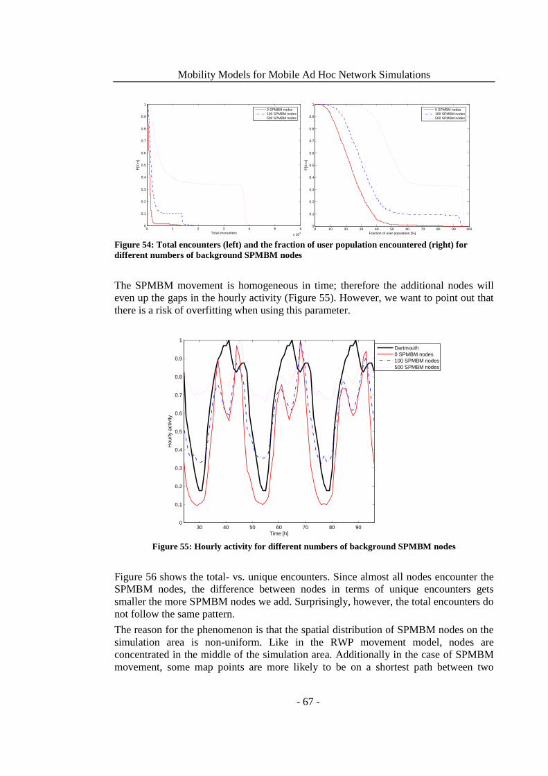
Mobility Models for Mobile Ad Hoc Network Simulations
- 67 -
0 1 2 3 4 5 6
x 104
0
0.1
0.2
0.3
0.4
0.5
0.6
0.7
0.8
0.9
1
P[X
>x]
Total encounters
0 SPMBM nodes100 SPMBM nodes500 SPMBM nodes
0 10 20 30 40 50 60 70 80 90 1000
0.1
0.2
0.3
0.4
0.5
0.6
0.7
0.8
0.9
1
P[X
>x]
Fraction of user population [%]
0 SPMBM nodes100 SPMBM nodes500 SPMBM nodes
Figure 54: Total encounters (left) and the fraction of user population encountered (right) for different numbers of background SPMBM nodes
The SPMBM movement is homogeneous in time; therefore the additional nodes will even up the gaps in the hourly activity (Figure 55). However, we want to point out that there is a risk of overfitting when using this parameter.
30 40 50 60 70 80 900
0.1
0.2
0.3
0.4
0.5
0.6
0.7
0.8
0.9
1
Time [h]
Hou
rly a
ctiv
ity
Dartmouth0 SPMBM nodes100 SPMBM nodes500 SPMBM nodes
Figure 55: Hourly activity for different numbers of background SPMBM nodes
Figure 56 shows the total- vs. unique encounters. Since almost all nodes encounter the SPMBM nodes, the difference between nodes in terms of unique encounters gets smaller the more SPMBM nodes we add. Surprisingly, however, the total encounters do not follow the same pattern.
The reason for the phenomenon is that the spatial distribution of SPMBM nodes on the simulation area is non-uniform. Like in the RWP movement model, nodes are concentrated in the middle of the simulation area. Additionally in the case of SPMBM movement, some map points are more likely to be on a shortest path between two

Mobility Models for Mobile Ad Hoc Network Simulations
- 68 -
arbitrarily selected map points. Hence, nodes sleeping, working and meeting their friends at map points with more traffic will naturally encounter more SPMBM nodes.
By only looking at the differences between nodes in terms of the proportion between unique and total encounter, the movement looks heterogeneous. Nevertheless, the SPMBM movement is a homogeneous model and it is only the combined effect that introduces heterogeneity. In other words, we can conclude that a hybrid model, combining a model having a non-uniform spatial distribution of nodes with another model with node movement restricted to different areas, can increase heterogeneity.
101
102
103
104
105
101
102
103
Uni
que
enco
unte
rs
Total encounters10
110
210
310
410
510
1
102
103
Uni
que
enco
unte
rs
Total encounters10
110
210
310
410
510
1
102
103
Uni
que
enco
unte
rs
Total encounters Figure 56: Total vs. unique encounters for 0 SPMBM nodes (left), 100 SPMBM nodes (middle) and 500 SPMBM nodes (right)
To give an idea of the sensitivity of the performance to this parameter, we show the results of the epidemic routing protocol simulations in Figure 57. Part of the performance gain in the scenarios with more SPMBM is due to a higher node density. However, the performance is better in the scenario with 500 SPMBM nodes than in the density experiment with 2000 nodes, so the SPMBM nodes do have a clear impact.
Figure 57: Performance of the Epidemic routing protocol for different numbers of background SPMBM nodes
The most important question still remains: Do the additional SPMBM background nodes increase the realism of the model. In the real world, there is not any background movement. All movement originates from people’s needs, which are complicated and not possible to model in detail. Therefore, an abstraction is necessary. But the SPMBM model may be too simple for this use.
6.2.12 Differences in schedules To get an understanding of the impact of the differences in schedules people have, we conducted the following experiment. We ran two scenarios: one where all nodes woke
Latency
0
10000
20000
30000
40000
50000
0 SPMBM Default 100 SPMBM 500 SPMBM
HopCount
0
2
4
6
8
10
0 SPMBM Default 100 SPMBM 500 SPMBM
Delivery ratio
0.0%
20.0%
40.0%
60.0%
80.0%
100.0%
0 SPMBM Default 100 SPMBM 500 SPMBM
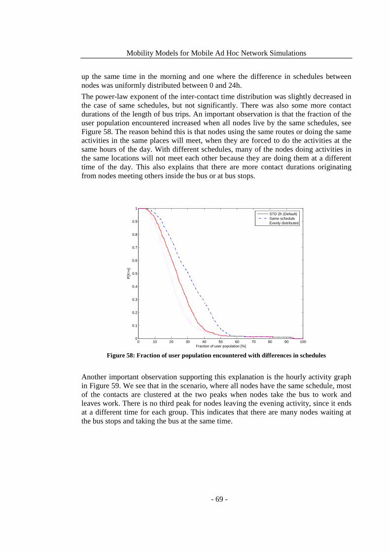
Mobility Models for Mobile Ad Hoc Network Simulations
- 69 -
up the same time in the morning and one where the difference in schedules between nodes was uniformly distributed between 0 and 24h.
The power-law exponent of the inter-contact time distribution was slightly decreased in the case of same schedules, but not significantly. There was also some more contact durations of the length of bus trips. An important observation is that the fraction of the user population encountered increased when all nodes live by the same schedules, see Figure 58. The reason behind this is that nodes using the same routes or doing the same activities in the same places will meet, when they are forced to do the activities at the same hours of the day. With different schedules, many of the nodes doing activities in the same locations will not meet each other because they are doing them at a different time of the day. This also explains that there are more contact durations originating from nodes meeting others inside the bus or at bus stops.
0 10 20 30 40 50 60 70 80 90 1000
0.1
0.2
0.3
0.4
0.5
0.6
0.7
0.8
0.9
1
P[X
>x]
Fraction of user population [%]
STD 2h (Default)Same scheduleEvenly distributed
Figure 58: Fraction of user population encountered with differences in schedules
Another important observation supporting this explanation is the hourly activity graph in Figure 59. We see that in the scenario, where all nodes have the same schedule, most of the contacts are clustered at the two peaks when nodes take the bus to work and leaves work. There is no third peak for nodes leaving the evening activity, since it ends at a different time for each group. This indicates that there are many nodes waiting at the bus stops and taking the bus at the same time.

Mobility Models for Mobile Ad Hoc Network Simulations
- 70 -
30 40 50 60 70 80 900
0.1
0.2
0.3
0.4
0.5
0.6
0.7
0.8
0.9
1
Time [h]
Hou
rly a
ctiv
ity
Dartmouth8h (Default)12hEvenly distributed
Figure 59: Hourly activity with differences in schedules
Figure 60 shows the results from the simulation of the epidemic routing protocol. Surprisingly, this parameter did not have an impact on the performance. However, this does not indicate that the parameter is useless. Our TTL was set to so high in the scenario, where all nodes have the same schedule, that packets sent during the night can get delivered during the next day. With a short TTL, most of the packets sent during the night are lost since there is no movement when all nodes are sleeping.
Figure 60: Performance of the Epidemic routing protocol for differences in schedules
6.2.13 Work times We conducted experiments with different lengths of work time. The two scenarios have 12h workday length and 4h workday length, which we compare to the default scenario which has 8h workday length.
The impact on the inter-contact times, contact durations, total- and unique encounters was negligible. Figure 61 shows that long workdays imply longer lasting activity.
Latency
0
10000
20000
30000
40000
50000
Diff 0s Default Evenly distributed
HopCount
0123456789
Diff 0s Default Evenly distributed
Delivery ratio
0.0%
20.0%
40.0%
60.0%
80.0%
100.0%
Diff 0s Default Evenly distributed

Mobility Models for Mobile Ad Hoc Network Simulations
- 71 -
30 40 50 60 70 80 900
0.1
0.2
0.3
0.4
0.5
0.6
0.7
0.8
0.9
1
Time [h]
Hou
rly a
ctiv
ity
DartmouthDefault12h4h
Figure 61: Hourly activity with different work time s
Figure 62 illustrates the performance of the epidemic routing protocol under the two conditions and the default scenario. Longer workdays imply shorter time spent at home, which leads to more contacts. Therefore, a performance gain is expected when increasing the workday length.
Figure 62: Performance of the Epidemic routing protocol for different work times
6.3 Summary In this chapter we validated the Working Day Movement model by showing that it produces similar distributions of inter-contact times and contact durations as the iMote trace, the contact patterns are heterogeneous and it has a similar periodic nature as the Dartmouth trace. Additionally, we studied the impact of the most important parameters.
Latency
0
10000
20000
30000
40000
50000
60000
43000s Default 14400s
HopCount
0123456789
43000s Default 14400s
Delivery ratio
0.0%
20.0%
40.0%
60.0%
80.0%
100.0%
43000s Default 14400s

Mobility Models for Mobile Ad Hoc Network Simulations
- 72 -
7 Discussion
This chapter begins by presenting the most important findings, following with advice how to configure the model and deal with complexity. Finally, limitations of the model and the experiments are discussed.
7.1 Major findings One important consideration that came up during this study is that metrics used in comparisons should be collected by similar methodologies both in simulations and real world measurements. Real world measurements have certain limitations, such as Bluetooth setup delays, too specific target groups chosen or geographical coordinates derived from WLAN access point data. When evaluating a model or fine-tuning some parameters to better fit a specific environment, researchers should collect metrics from the simulation in the same manner as they were collected in the real world experiments used for validation. For example, if the node locations in a real world movement trace were calculated from access point data, access points should also be modeled in the simulation when data is collected.
Regarding the different parameters of the model, we found that in terms of our collected metrics the geometry of the map has a small impact on mobility compared to many other configurable properties of our model (Section 6.2.4). Therefore, when modeling a specific environment with our model, researchers should concentrate more on other characteristics of the environment than the road net.
Additionally, we were also able to demonstrate that pause times in the office movement can be used to configure an appropriate power-law exponent of the fist 12h part of the inter-contact times distribution (Section 6.2.7). Furthermore, we showed that the parameter controlling the probability to do evening activity (Chapter 6.2.8) together with the work day length (Chapter 6.2.13) can be used to vary the level of contact activity among nodes at each hour. Moreover, we showed that the use of districts is a good way to limit node movement and the fraction of the user population a node encounters (Chapter 6.2.3). Finally, we observed that some parameters have such a small impact that they need not be taken into consideration when modeling a specific environment and can probably even be removed in future versions.

Mobility Models for Mobile Ad Hoc Network Simulations
- 73 -
7.2 Configuration When running simulations with our movement model, a warmup time of 43000s (~12h) must be used for the mobility model to reach a stationary state. The reason behind this is that each node’s initial location is its home, where it starts in the sleeping mode. Because nodes are living according to different schedules, the wakeup time for the first day can vary between −43000 and 43000; hence, it is important to give the nodes an opportunity to wake up at their right time. Without a warmup time, half of the nodes would wake up immediately when the simulation starts. Another warmup time is also needed for the network load to reach a stable state. This depends on the protocols that are simulated and their settings, and is not covered here.
The way to set up the map and choose which nodes or areas are included in the simulation depends completely on the use case. If we are interested in knowing how well a new DTN instant messaging application works within the Helsinki center area, we might want to create areas for the center and the surrounding districts and create some amount of nodes to each area. When measuring delay, packet delivery ratio and similar metrics, we only log events from nodes belonging to the Helsinki center group, or we create another group inside the same area which we monitor. All the other nodes from other groups will of course send and carry packets too, but these are not taken into account in the results. The alternative, to create a separate group for the test subjects, is preferable since we might want to have different message sending patterns for the users of the instant messaging application. But the sending of messages is not part of the mobility model and therefore a topic for another discussion.
To better illustrate the idea of using a specific district for simulations of protocols and applications, we give an example using Figure 5 (Page 23) again. In this example, we use nodes belonging to district D6 as our target group. Most of the nodes belonging to D1 district can be seen as drive through traffic, while nodes belonging to D2–D5 have activities both in D6 and elsewhere. Some nodes are living elsewhere but only coming to D6 to work or meet friends, others are living in D6 but working elsewhere. Some nodes are never entering D6, but are an important part of the mobility since they will generate packets that will fill buffer space of nodes within the D6 district. When measuring latency, delivery ratio and other performance metrics, we only log packets sent or received by pure D6 nodes, i.e. nodes belonging to the D6 group that never leave the D6 district.
Without these extra nodes, even though we only focus on a specific group of test subjects in our simulations, all packets travelling inside the D6 simulation area are sent from D6 nodes and destined to D6 nodes. Buffer capacity is an important constraint in ad hoc networks; therefore, it is very important to have other packets than the ones sent or destined to D6 nodes carried around in the network, too. Otherwise, simulations would show that protocols with unrealistically little buffer space allocated for nodes are successful.
It is important to note that even though one should only focus on a specific group of nodes within a specific area during simulations of actual protocols or applications, it is different when one is validating a model. For example if we want to verify that the inter-contact times in some specific town are power-law distributed with some experimentally determined coefficient, we consider all nodes. However, one can argue

Mobility Models for Mobile Ad Hoc Network Simulations
- 74 -
that the distribution of inter-contact times in real world experiments, too, depends on how the contacts were measured. If we know how the inter-contact times were measured in the real world experiments, we can use a similar methodology in the simulation, too. According to a study [31], the pair wise inter-contact times are very different between node pairs. Results can be different depending on how the focus group is selected, due to this heterogeneity.
7.3 Generating configurations The downside of a model capturing movement of nodes at level of detail like ours is that it introduces a certain degree of complexity in terms of configuration. Specifying where thousands of nodes live and work is not feasible to do manually. Even more challenging is the process of obtaining reliable data for all the different parameters like people's schedules, where they work and which buses they use. Therefore, when researchers model specific environments with the help of our model, we advise them to create settings and other data files with the help of scripts. These scripts could take fewer parameters as input, thereby reducing the complexity.
A model capturing movement of nodes at a detailed level must make a tradeoff between configurability and ease of use. Scripts taking as input only a few parameters from which the parameters of the real model can be derived from are easier to work with and thus more practical. Some statistical data, like residential density within different areas of a city, might be available to researchers; hence, a script can place homes and offices accordingly while randomizing the rest. Currently, if homes, offices or meeting spots are not configured by the user, they are all uniformly distributed over the map.
7.4 Limitations of the model Like every model, we need to provide an abstraction of reality to maintain the complexity at an acceptable level. All of the activities are modeled at a high level with simple abstractions on a two dimensional plane. Floors, walls and different obstacles affect mobility and especially the contacts between nodes, but are not covered in our model. A real working day exhibits more subtleties than we currently cover, including, e.g., lunch breaks and shopping activities. Furthermore, in our experiments, devices are always turned on. Even though modeling of attenuation and on/off times is not a responsibility of the mobility model, it is worth noting that measurements from real user traces, typically used for validation of mobility models, have been affected by these details.
While these are not included in our current model and implementation, further submodels can be added for more fine-grained capturing of daily activities and parameterization allows further fine-tuning. Similarly, on/off periods can be added by revising the corresponding mechanisms available in the ONE.
7.4.1 Buildings and dimensions The lack of a z-dimension in our model is one of the biggest limitations. A real building with many floors can occupy a very small area in a city, but still have plenty of space to walk in and room for a huge amount of people. It is possible to increase the office size to compensate for the lack of floors. However, the contact patterns at a real office will
Mobility Models for Mobile Ad Hoc Network Simulations
- 75 -
still be different due to walls, corridors and floors, restricting nodes from being in contact with each other.
Another shortcoming with the way movement inside buildings is modeled is that nodes moving at the edges of the office will be in contact with nodes moving on the street. It is also possible that a large building is placed within a too small block on the map, resulting in a situation where there goes a road through the office, again generating unrealistic connections between nodes inside the office and nodes walking on streets. Both of these errors can be avoided if walls are modeled.
One idea is to create an abstraction of the buildings, by separating the buildings completely from the map, so that the nodes inside buildings are temporarily removed from the map. Some high level algorithm can determine when nodes are in contact, or the office scenario can be modeled separately within another map.
7.4.2 Traffic We do not model traffic in the sense of queues, traffic lights, or speed limits. This is necessary to model since during the stops at traffic lights, other nodes have good chances to transmit data. If cars are moving with a high speed all the time, other nodes might not get an opportunity to send anything.
Another limitation is that roads do not have any width so all nodes are moving along the same path. Buses and people at the same stop are modeled to be standing at the exact same location; therefore all of them are in contact with each other. Since bus frames do not attenuate signals, nodes inside the bus will be in contact with other nodes outside.
The group movement during the evening activity is also modeled in the way that all nodes are at the exact same location. This is different from reality since groups of people usually get scattered every now and then.
Finally, nodes are always moving according to the shortest path. In the real world, people are often using certain familiar streets, or choose a specific path for other reasons. Especially cars are rarely moving according to the shortest path. Main roads and highways are preferred due to higher speed limits. A first step towards this goal would be to implement a noisy Dijkstra’s algorithm, which overlooks a specific portion of the links in the graph.
7.4.3 Implementation The implementation of the model can also be improved to enhance the performance of the simulation. Even though the movement model is not the biggest bottleneck at the time of writing, it may be when several issues related to packet forwarding have been addressed.
Every time a node moves from one location to the other, Dijkstra’s algorithm is used to calculate the shortest path. One idea is to cache often calculated minimal spanning trees. Most of the paths will either begin or end at a bus stop, therefore one idea is to store the minimal spanning tree from each bus stop.
Small improvements can be made to the design by extracting a generic abstract ActivityMovement class, encompassing aspects from all three activity classes.

Mobility Models for Mobile Ad Hoc Network Simulations
- 76 -
Likewise, a generic abstract ControlSystem class can be designed to make it easier for new developers to create activities requiring synchronization between several different entities. For example, if traffic is to be modeled in more detail all vehicles like cars and buses must be aware of each other, in order to not drive through each other. A control system for this can be used.
The MovementModel class’ interface to the DTNHost is misplaced. The responsibility of moving nodes in terms of updating the coordinates should be at the movement model. The MovementModel should communicate with the DTNHost solely by giving the new coordinates of the node. The current interface where paths and wait times are delivered by the movement model when asked introduces high coupling and low cohesion.
There is a small defect in the group movement part of the evening activity. With certain parameters (few nodes, small differences in schedules and many meeting spots), a group may not become full during the day, resulting in the group waiting for the last member until the next day before it can take off and start walking. This will not occur normally since nodes are moving according to different schedules so there will always be someone to fill the last slot. A possible fix is to trigger group walk after nodes have waited a certain time.
7.5 Limitations of the results The real world data used for the validation of our model is too limited. We had only access to three different metrics: inter-contact times, contact durations and hourly activity. It is possible to create lots of different models producing similar results when these metrics are compared; therefore, we cannot say if we are overfitting our model. Even if the metrics were sufficient, they would be obtained from different traces (Dartmouth and iMote traces). Additionally, different measurement practices were used in both these experiments and the simulation. Hence, we can only say that the model has certain real world characteristics like power-law distribution of inter-contact times up to 12h and repetitiveness in time.
We only studied the impact of each parameter separately. A full exploration of the parameter space would require each combination to be simulated, too.
The used metrics are not sufficient to characterize mobility. As we saw, there were a few parameters that can be changed without causing many differences in the metrics, but still having an impact on the performance of the Epidemic routing protocol.
Using the Epidemic routing protocol for sensitivity analysis the way we did also has some drawbacks. We selected our bandwidth and packet sizes so that nodes would not have time to transfer all their packets during the shorter contacts. The idea was to capture this, together with the overall connectivity, as one result. However, the problem is that it is not possible to distinguish between these when only measuring packet delivery ratio and latency. A low packet delivery ratio can be a result of bad connectivity or too short contacts. A better solution is to run two different simulations; one where the bandwidth and packet size are set so that nodes can always transfer all their packets during a short contact, the other where packets are of different sizes. For

Mobility Models for Mobile Ad Hoc Network Simulations
- 77 -
the latter, we can draw a graph with the delivery ratio (or latency) as a function of the packet size.
Finally, comparison of our model to real world traces in terms of routing protocol performance would have served as a final test. However, this is not possible due to certain limitations in the traces.
First of all, real user traces are all too limited. Recall that the iMote traces included contacts between two iMotes and between iMotes and other Bluetooth devices. Suppose we simulated the Epidemic routing protocol, in a scenario where the iMote nodes are sending packets to other iMote nodes between evenly distributed time intervals. In this case, all the iMote nodes are researchers of the same group and therefore their connection patterns to each other are very specific. Even though two iMote nodes would not meet each other, routing could not go through other nodes as well, since all connections between two non-iMote devices are missing from the trace.
The Dartmouth trace is restricted to a specific area. Unfortunately, many of the nodes only visit the network on few rare occasions. Therefore, message generation in the simulation must take this to account. For example, let us assume that we have been collecting a trace during the whole January. When we use the trace in our simulation, if node A has only visited the network on the 6th day and node B tries to send a message to A on the 15th day, the message cannot be delivered even though node A would have been within reach in the real world. This is a result of the boundary effect. It is not much better if we only allow nodes that are inside the simulation area most of the time to send packets to each other. This is because the shortest, or in some cases the only, path of a message is one going outside the simulation area. Additionally, nodes coming into the simulation area should not have empty buffers. It is difficult to simulate a routing protocol with a set of traces so that comparison with the results from a similar simulation with a synthetic model is meaningful.
Another smaller shortcoming with using the performance of an existing routing protocol as a metric for comparison is that some futuristic routing protocols can make use of some mobility characteristics that we do not know about today. Routing protocols utilizing these characteristics will perform differently if these characteristics are not captured in the model. However, the inter-contact times, contact-durations and the other metrics do not capture the movement any better either, so using the performance metric as an additional metric is a good idea if there is data to support it.
A final consideration regarding the routing protocol simulations is the sending of packets. Instead of just having nodes randomly sending messages to each other, a better solution would have been to have nodes sending broadcast messages and measure the delivery ratio and latency of a broadcast message. This metric correlates better with the overall connectivity of the network.
7.6 Summary In this chapter we discussed the major findings from our study. We also gave advice how to configure the model for different experiments and how to deal with the complexity of the model. Finally, we discussed the limitations of the model and the reliability of the results obtained from simulations.

Mobility Models for Mobile Ad Hoc Network Simulations
- 78 -
8 Conclusions
We have developed a new mobility model using a submodel approach, where each submodel handles some activity people do; staying at home, working at an office, going out with friends in the evening and moving between activities. The new model captures several different mobility characteristics at a lower level of abstraction than many other models have so far. We have shown that the model is heterogeneous in both time and space and produces similar distributions of inter-contact times and contact durations as real user traces. Additionally, we have explored how altering parameters of our model affect mobility by comparison in terms of several different metrics.
The approach to increase the reality by modeling movement in more detail has two shortcomings. The first one is that reliable validation of the model is not possible due to lack of available real world data for comparisons. The second shortcoming is that many of the metrics used in comparisons encompass other than mobility characteristics, too. In order to increase the reality we must know more about what realistic movement is and we must have good procedures for verifications. Therefore, at this early stage of DTN, research in the field of characterization of movement and measurement of real user movement may provide better contributions to the research community than the design of new realistic movement models.
8.1 Future work Possible next steps are to implement additional submodels and further develop the old ones. Modeling of traffic at a more detailed level is also an important extension. Furthermore, we have plans to develop scripts and tools to better handle the complexity and also to conduct experiments to explore the parameter space in hope of eliminating redundant parameters. Finally, one idea is to develop mechanisms to simulate the recording of a trace with the same procedures as has been used in the real world experiments; thereby obtaining results more valuable for validation of a model.
At the moment, roads do not have any width, and nodes at bus stops or moving in group are at the exact same spot. A possible extension to overcome this limitation is to introduce the concept of physical- and logical location. Movement models’ getPath() method could convert each coordinate in the path according to some rules depending on

Mobility Models for Mobile Ad Hoc Network Simulations
- 79 -
the model and the current state. For example, the evening activity could adjust each coordinate in the path with a value drawn from some specific distribution, resulting in the group being looser. Nodes moving in a bus could select a specific coordinate for the whole bus trip. The coordinate would correspond to the node’s seat and is proportional to the bus’ coordinate. We showed that the way nodes move between activities have a huge impact and is thus important to model accurately. Therefore, we believe that it is worth to develop more accurate transportation movement submodels in the future.
In addition to accurate modeling of the movement of nodes, message sending patterns and attenuation should be modeled as well. The reason they are mentioned here is that they have certain dependencies to the movement, and vice versa.
The sending patterns are largely application dependent. However, people tend to use certain applications in different areas or during different activities. Additionally, the node pairs communicating with each other are usually socially connected to each other; they may be friends from work or neighbors. Hence, a successful message generation module must be aware of the relationships between nodes and what activities nodes are doing.
Walls and other obstacles are both attenuating the signal and restricting movement, so the walls cannot be solely encapsulated into one module. Walls, buildings and other obstacles can be encapsulated into a separate world module to which other modules have access to. But the issue with sending patterns is not as easily solved. One idea is to create a node behavior black box constituting both node movement and sending of messages.
Further research is needed in the field of characterizing movement. The idea to come up with one metric characterizing movement is probably going to be an endless search; meanwhile, we can experiment with new metrics defining other aspects of mobility. One topic is to find a good way to measure heterogeneity. If measured with contacts, one can use the variance of the angle of the line from origin to a dot on the log-log scatter diagram. Another option is to take into account other properties than just contacts. A general improvement of the metric is to measure the number of total and unique encounters during a specific time interval, in order to have more comparable results.
This suggests future research to come up with a movement model characterization and comparison framework, since one metric is unlikely to be able to describe movement. Finally, there is a need for more real world data from different environments for comparisons.
8.2 Final words Simulations cannot replace real world experiments, and the movement of the nodes is just one property that needs to be modeled. Due to lack of available data for verification, it is not possible to say how well different environments can be modeled with our model. However, protocol simulations with the model configured with different parameters can provide another insight of how well the protocol performs under different conditions.

Mobility Models for Mobile Ad Hoc Network Simulations
- 80 -
Another important question is whether the differences between target environments are so huge that a single model, being the lowest common denominator of all different scenarios, differs from each real environment as much as the RWP? If this is the case, simple models, configured with all extreme values for the parameters, can as well be used for simulations.
At the moment, the best approach for DTN protocol and application developers is to run their simulations with different models configured with different parameters, keeping in mind that simulations cannot replace real world experiments.

Mobility Models for Mobile Ad Hoc Network Simulations
- 81 -
References
[1] Tracy Camp, Jeff Boleng, and Vanessa Davies. A survey of mobility models for ad hoc network research. Wireless Communications and Mobile Computing, 2(5): 483–502, 2002.
[2] E. P. Jones and P. A. Ward, Routing strategies for delay-tolerant networks, In Proceedings of ACM SIGCOMM, 2004.
[3] Vinton G. Cerf, Scott C. Burleigh, Robert C. Durst, and Dr. Kevin Fall. Delay-Tolerant Network Architecture. http://www.ietf.org/internetdrafts/draft-irtf-dtnrg-arch-02.txt, 2004.
[4] Thomas Clausen and Philippe Jacquet. Optimized link state routing protocol (olsr). RFC 3626, Internet Engineering Task Force, October 2003.
[5] Charles E. Perkins, Elizabeth M. Belding-Royer, and Samir R. Das. Ad hoc on-demand distance vector (aodv) routing. RFC Experimental 3561, Internet Engineering Task Force, July 2003.
[6] Jeremie Leguay, Timur Friedman, and Vania Conan. Evaluating mobility pattern space routing for dtns. In INFOCOM. IEEE, 2006.
[7] Sushant Jain, Kevin R. Fall, and Rabin K. Patra. Routing in a delay tolerant network. In Raj Yavatkar, Ellen W. Zegura, and Jennifer Rexford, editors, SIGCOMM, pages 145–158. ACM, 2004.

Mobility Models for Mobile Ad Hoc Network Simulations
- 82 -
[8] Ari Keränen and Jörg Ott. Increasing reality for DTN protocol simulations. Technical Report, Helsinki University of Technology, Networking Laboratory, July 2007.
[9] Augustin Chaintreau, Pan Hui, Jon Crowcroft, Christophe Diot, Richard Gass, and James Scott. Pocket switched networks: Real-world mobility and its consequences for opportunistic forwarding. Technical Report UCAM-CL-TR-617, University of Cambridge, Computer Laboratory, February 2005.
[10] Augustin Chaintreau, Pan Hui, Jon Crowcroft, Christophe Diot, Richard Gass, and James Scott. Impact of human mobility on the design of opportunistic forwarding algorithms. In Proc. INFOCOM'06, 2006.
[11] Thomas Karagiannis, Jean-Yves Le Boudec, and Milan Vojnovic. Power law and exponential decay of inter contact times between mobile devices. In Evangelos Kranakis, Jennifer C. Hou, and Ram Ramanathan, editors, Proc. MOBICOM'07, pages 183–194, 2007.
[12] Marvin McNett and Geoffrey M. Voelker. Access and mobility of wireless pda users. Mobile Computing and Communications Review, 9(2):40–55, 2005.
[13] Tristan Henderson, David Kotz, and Ilya Abyzov. The changing usage of a mature campus-wide wireless network. In Zygmunt J. Haas, Samir R. Das, and Ravi Jain, editors, MOBICOM, pages 187–201. ACM, 2004.
[14] James Scott, Richard Gass, Jon Crowcroft, Pan Hui, Christophe Diot, and Augustin Chaintreau. CRAWDAD trace cambridge/haggle/imote/infocom (v. 2006-01-31). Downloaded from http://crawdad.cs.dartmouth.edu/cambridge/ haggle/imote/infocom, January 2006.
[15] Minkyong Kim, David Kotz, and Songkuk Kim. Extracting a mobility model from real user traces. In Proc. INFOCOM'06, 2006. Downloaded from http://nile.usc.edu/MobiLib/USC_trace_intro.html.
[16] Wei-jen Hsu and Ahmed Helmy. Description of the USC wireless LAN traces. Web page. Referenced May 7, 2008. Last updated: Aug. 12, 2005.
[17] Mirco Musolesi and Cecilia Mascolo. A community based mobility model for ad hoc network research. In Proc. 2nd ACM/SIGMOBILE International Workshop on Multi-hop Ad Hoc Networks: from theory to reality (REALMAN'06), May 2006.

Mobility Models for Mobile Ad Hoc Network Simulations
- 83 -
[18] David B Johnson and David A Maltz. Dynamic source routing in ad hoc wireless networks. In Imielinski and Korth, editors, Mobile Computing, volume 353. Kluwer Academic Publishers, 1996.
[19] Han Cai and Do Young Eun. Crossing over the bounded domain: from exponential to power-law inter-meeting time in manet. In Evangelos Kranakis, Jennifer C. Hou, and Ram Ramanathan, editors, MOBICOM, pages 159–170. ACM, 2007.
[20] Jungkeun Yoon, Mingyan Liu, and Brian Noble. Random waypoint considered harmful. In INFOCOM, 2003.
[21] Injong Rhee, Minsu Shin, Seongik Hong, Kyunghan Lee, and Song Chong. On the Levy-walk nature of human mobility: Do humans walk like monkeys? Technical Report, North Carolina State University, 2007.
[22] Wei jen Hsu, Thrasyvoulos Spyropoulos, Konstantinos Psounis, and Ahmed Helmy. Modeling time-variant user mobility in wireless mobile networks. In Proc. INFOCOM'07, pages 758–766, 2007.
[23] Daniel Minder, Pedro José Marrón, Andreas Lachenmann, and Kurt Rothermel. Experimental construction of a meeting model for smart office environments. In Proc. First Workshop on Real-World Wireless Sensor Networks (REALWSN 2005), SICS Technical Report T2005:09, June 2005.
[24] J. Habetha, M. Nadler, and d. Calvo. Dynamic clustering with quality of service guarantees and forwarder selection in wireless ad hoc networks. In Proc. Asia Pacific Conference on Communications, Seoul, Korea, November 2000.
[25] X. Hog, M. Gerla, G. Pei, and C.-C. Chiang. A group mobility model for ad hoc wireless networks. In Proc. ACM/IEEE MSWiM '99, Seattle, WA, August 1999.
[26] Wei jen Hsu and Ahmed Helmy. IMPACT: Investigation of mobile-user patterns across university campuses using WLAN trace analysis. CoRR, abs/cs/0508009, 2005. informal publication.
[27] John Burgess, Brian Gallagher, David Jensen, and Brian Neil Levine. Maxprop: Routing for vehicle-based disruption-tolerant networks. In INFOCOM. IEEE, 2006.

Mobility Models for Mobile Ad Hoc Network Simulations
- 84 -
[28] Libo Song and David F. Kotz. Evaluating opportunistic routing protocols with large realistic contact traces. In Proc. CHANTS'07, pages 35–42, New York, NY, USA, 2007.
[29] David Kotz, Tristan Henderson, and Ilya Abyzov. CRAWDAD trace dartmouth/campus/syslog/01_04 (v. 2004-12-18). Downloaded from http://crawdad.cs.dartmouth.edu/dartmouth/campus/syslog/0104, December2004.
[30] Wei Wang, Vikram Srinivasan, and Mehul Motani. Adaptive contact probing mechanisms for delay tolerant applications. In Evangelos Kranakis, Jennifer C. Hou, and Ram Ramanathan, editors, MOBICOM, pages 230–241. ACM, 2007.
[31] Vania Conan, Jérémie Leguay, and Timur Friedman. Characterizing pairwise inter-contact patterns in delay tolerant networks. In Autonomics '07 Proceedings of the 1st international conference on Autonomic computing and communication systems, pages 1–9, ICST, Brussels, Belgium, Belgium, 2007. ICST (Institute for Computer Sciences, Social-Informatics and Telecommunications Engineering).
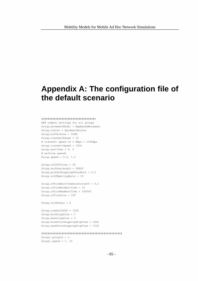
Mobility Models for Mobile Ad Hoc Network Simulations
- 85 -
Appendix A: The configuration file of the default scenario
###################################
### common settings for all groups
Group.movementModel = MapBasedMovement
Group.router = EpidemicRouter
Group.bufferSize = 100M
Group.transmitRange = 10
# transmit speed of 2 Mbps = 250kBps
Group.transmitSpeed = 100k
Group.waitTime = 0, 0
# walking speeds
Group.speed = 0.5, 1.5
Group.nrOfOffices = 50
Group.workDayLength = 28800
Group.probGoShoppingAfterWork = 0.5
Group.nrOfMeetingSpots = 10
Group.officeWaitTimeParetoCoeff = 0.5
Group.officeMinWaitTime = 10
Group.officeMaxWaitTime = 100000
Group.officeSize = 100
Group.nrofHosts = 0
Group.timeDiffSTD = 7200
Group.minGroupSize = 1
Group.maxGroupSize = 3
Group.minAfterShoppingStopTime = 3600
Group.maxAfterShoppingStopTime = 7200
################################################### #
Group1.groupID = o
Group1.speed = 7, 10

Mobility Models for Mobile Ad Hoc Network Simulations
- 86 -
Group1.waitTime = 10, 30
Group1.nrofHosts = 2
Group1.movementModel = BusMovementModel
Group1.routeFile = data/HelsinkiMedium/A_bus.wkt
Group1.routeType = 2
Group1.busControlSystemNr = 1
Group2.groupID = A
Group2.waitTime = 0, 0
Group2.nrofHosts = 150
Group2.movementModel = DailyRoutinesMovement
Group2.busControlSystemNr = 1
Group2.speed = 0.8, 1.4
Group2.ownCarProb = 0.5
Group2.shoppingControlSystemNr = 1
Group2.meetingSpotsFile = data/HelsinkiMedium/A_mee tingspots.wkt
Group2.officeLocationsFile = data/HelsinkiMedium/A_ offices.wkt
Group2.homeLocationsFile = data/HelsinkiMedium/A_ho mes.wkt
Group3.groupID = p
Group3.speed = 7, 10
Group3.waitTime = 10, 30
Group3.nrofHosts = 2
Group3.movementModel = BusMovementModel
Group3.routeFile = data/HelsinkiMedium/B_bus.wkt
Group3.routeType = 2
Group3.busControlSystemNr = 2
Group4.groupID = B
Group4.waitTime = 0, 0
Group4.nrofHosts = 50
Group4.movementModel = DailyRoutinesMovement
Group4.busControlSystemNr = 2
Group4.speed = 0.8, 1.4
Group4.ownCarProb = 0.5
Group4.shoppingControlSystemNr = 2
Group4.meetingSpotsFile = data/HelsinkiMedium/B_mee tingspots.wkt
Group4.officeLocationsFile = data/HelsinkiMedium/B_ offices.wkt
Group4.homeLocationsFile = data/HelsinkiMedium/B_ho mes.wkt
Group5.groupID = q
Group5.speed = 7, 10
Group5.waitTime = 10, 30
Group5.nrofHosts = 2
Group5.movementModel = BusMovementModel
Group5.routeFile = data/HelsinkiMedium/C_bus.wkt
Group5.routeType = 2
Group5.busControlSystemNr = 3
Group6.groupID = C
Group6.waitTime = 0, 0
Group6.nrofHosts = 100
Group6.movementModel = DailyRoutinesMovement
Group6.busControlSystemNr = 3
Group6.speed = 0.8, 1.4

Mobility Models for Mobile Ad Hoc Network Simulations
- 87 -
Group6.ownCarProb = 0.5
Group6.shoppingControlSystemNr = 3
Group6.meetingSpotsFile = data/HelsinkiMedium/C_mee tingspots.wkt
Group6.officeLocationsFile = data/HelsinkiMedium/C_ offices.wkt
Group6.homeLocationsFile = data/HelsinkiMedium/C_ho mes.wkt
Group7.groupID = r
Group7.speed = 7, 10
Group7.waitTime = 10, 30
Group7.nrofHosts = 2
Group7.movementModel = BusMovementModel
Group7.routeFile = data/HelsinkiMedium/D_bus.wkt
Group7.routeType = 2
Group7.busControlSystemNr = 4
Group8.groupID = D
Group8.waitTime = 0, 0
Group8.nrofHosts = 100
Group8.movementModel = DailyRoutinesMovement
Group8.busControlSystemNr = 4
Group8.speed = 0.8, 1.4
Group8.ownCarProb = 0.5
Group8.shoppingControlSystemNr = 4
Group8.meetingSpotsFile = data/HelsinkiMedium/D_mee tingspots.wkt
Group8.officeLocationsFile = data/HelsinkiMedium/D_ offices.wkt
Group8.homeLocationsFile = data/HelsinkiMedium/D_ho mes.wkt
Group9.groupID = s
Group9.speed = 7, 10
Group9.waitTime = 10, 30
Group9.nrofHosts = 2
Group9.movementModel = BusMovementModel
Group9.routeFile = data/HelsinkiMedium/E_bus.wkt
Group9.routeType = 2
Group9.busControlSystemNr = 5
Group10.groupID = E
Group10.waitTime = 0, 0
Group10.nrofHosts = 100
Group10.movementModel = DailyRoutinesMovement
Group10.busControlSystemNr = 5
Group10.speed = 0.8, 1.4
Group10.ownCarProb = 0.5
Group10.shoppingControlSystemNr = 5
Group10.meetingSpotsFile = data/HelsinkiMedium/E_me etingspots.wkt
Group10.officeLocationsFile = data/HelsinkiMedium/E _offices.wkt
Group10.homeLocationsFile = data/HelsinkiMedium/E_h omes.wkt
Group11.groupID = t
Group11.speed = 7, 10
Group11.waitTime = 10, 30
Group11.nrofHosts = 2
Group11.movementModel = BusMovementModel
Group11.routeFile = data/HelsinkiMedium/F_bus.wkt
Group11.routeType = 2
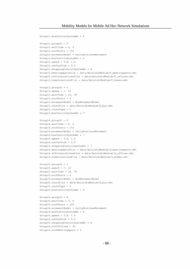
Mobility Models for Mobile Ad Hoc Network Simulations
- 88 -
Group11.busControlSystemNr = 6
Group12.groupID = F
Group12.waitTime = 0, 0
Group12.nrofHosts = 150
Group12.movementModel = DailyRoutinesMovement
Group12.busControlSystemNr = 6
Group12.speed = 0.8, 1.4
Group12.ownCarProb = 0.5
Group12.shoppingControlSystemNr = 6
Group12.meetingSpotsFile = data/HelsinkiMedium/F_me etingspots.wkt
Group12.officeLocationsFile = data/HelsinkiMedium/F _offices.wkt
Group12.homeLocationsFile = data/HelsinkiMedium/F_h omes.wkt
Group13.groupID = u
Group13.speed = 7, 10
Group13.waitTime = 10, 30
Group13.nrofHosts = 2
Group13.movementModel = BusMovementModel
Group13.routeFile = data/HelsinkiMedium/G_bus.wkt
Group13.routeType = 2
Group13.busControlSystemNr = 7
Group14.groupID = G
Group14.waitTime = 0, 0
Group14.nrofHosts = 150
Group14.movementModel = DailyRoutinesMovement
Group14.busControlSystemNr = 7
Group14.speed = 0.8, 1.4
Group14.ownCarProb = 0.5
Group14.shoppingControlSystemNr = 7
Group14.meetingSpotsFile = data/HelsinkiMedium/G_me etingspots.wkt
Group14.officeLocationsFile = data/HelsinkiMedium/G _offices.wkt
Group14.homeLocationsFile = data/HelsinkiMedium/G_h omes.wkt
Group15.groupID = v
Group15.speed = 7, 10
Group15.waitTime = 10, 30
Group15.nrofHosts = 4
Group15.movementModel = BusMovementModel
Group15.routeFile = data/HelsinkiMedium/H_bus.wkt
Group15.routeType = 2
Group15.busControlSystemNr = 8
Group16.groupID = H
Group16.waitTime = 0, 0
Group16.nrofHosts = 200
Group16.movementModel = DailyRoutinesMovement
Group16.busControlSystemNr = 8
Group16.speed = 0.8, 1.4
Group16.ownCarProb = 0.5
Group16.shoppingControlSystemNr = 8
Group16.nrOfOffices = 40
Group16.nrOfMeetingSpots = 5

Mobility Models for Mobile Ad Hoc Network Simulations
- 89 -
Group17.groupID = K
Group17.movementModel = ShortestPathMapBasedMovemen t
Group17.waitTime = 100, 300
Group17.speed = 7, 10
Group17.nrofHosts = 10
# max number of external events to preload (default = 500)
ExternalEvents.nrofPreload = 500
# path to external events file
ExternalEvents.filePath = ee/700_events_1000_nodes_ 700ks.txt
# seed for movement models' pseudo random number ge nerator (default = 0)
MovementModel.rngSeed = [2; 8372; 98092; 18293; 777 ]
# World's size for Movement Models without implicit size (width, height; meters)
MovementModel.worldSize = 10000, 8000
# How long time to move hosts in the world before r eal simulation
MovementModel.warmup = 43000
## Map based movement -movement model specific sett ings
MapBasedMovement.nrofMapFiles = 1
MapBasedMovement.mapFile1 = data/HelsinkiMedium/roa ds.wkt
## Reports - all report names have to be valid repo rt classes
# how many reports to load
Report.nrofReports = 8
# default directory of reports (can be overriden pe r Report with output setting)
Report.reportDir = [reports/ORIGINAL/1; reports/ORI GINAL/2; reports/ORIGINAL/3; reports/ORIGINAL/4; reports/ORIGINAL/5]
# Report classes to load
Report.report1 = InterContactTimesReport
Report.report2 = ContactTimesReport
Report.report3 = UniqueEncountersReport
Report.report4 = TotalEncountersReport
Report.report5 = EncountersVSUniqueEncountersReport
Report.report6 = ContactsDuringAnICTReport
Report.report7 = MessageStatsReport
Report.report8 = ContactsPerHourReport
## Default settings for some routers settings
ProphetRouter.secondsInTimeUnit = 30
SprayAndWaitRouter.nrofCopies = 6
SprayAndWaitRouter.binaryMode = true
## Optimization settings -- these affect the speed of the simulation
## see World class for details.
Optimization.connectionAlg = 2
Optimization.cellSizeMult = 5
Optimization.randomizeUpdateOrder = true
## GUI settings
Mobility Models for Mobile Ad Hoc Network Simulations
- 90 -
# GUI underlay image settings
GUI.UnderlayImage.fileName = data/helsinki_underlay .png
# Image offset in pixels (x, y)
GUI.UnderlayImage.offset = 64, 20
# Scaling factor for the image
GUI.UnderlayImage.scale = 4.75
# Image rotation (radians)
GUI.UnderlayImage.rotate = -0.015
# how many events to show in the log panel (default = 30)
GUI.EventLogPanel.nrofEvents = 200
# Regular Expression log filter (see Pattern-class from the Java API for RE-matching details)
#GUI.EventLogPanel.REfilter = .*p[1-9]<->p[1-9]$