mobile robot map building from an advanced sonar...

Mobile Robot Map Building from an Advanced SonarArray and Accurate Odometry , MECSE-1996-10

1

Mobile Robot Map Building from an Advanced Sonar Array andAccurate Odometry

Kok Seng CHONG Lindsay [email protected] [email protected]

Intelligent Robotics Research Center (IRRC)Department of Electrical and Computer System Engineering

Monash University, Victoria 3168 Australiahttp://calvin.eng.monash.edu.au/IRRC/IRRCHomePage.html

AbstractThis paper describes a mobile robot equipped with a sonar sensor array in a guidedfeature based map building task in an indoor environment. The landmarks common toindoor environments are planes, corners and edges, and these are located and classifiedwith the sonar sensor array. The map building process makes use of accurate odometryinformation that is derived from a pair of knife edged unloaded encoder wheels. Discretesonar observations are incrementally merged into partial planes to produce a realisticrepresentation of environment that is amenable to sonar localisation. Collinearityconstraints among features are exploited to enhance both the map feature estimation androbot localisation. The map update employs an Iterated Extended Kalman Filter (IEKF)in the first implementation and subsequently a comparison is made with the Julier-Uhlmann Kalman Filter (JUKF) which improves the accuracy of covariance propagationwhen non-linear equations are involved. The map accounts for correlation among featuresand robot positions. Partial planes are also used to eliminate phantom targets caused byspecular reflection of the sonar. Unclassifiable sonar targets are integrated into the mapfor the purpose of obstacle avoidance. The paper presents simulated and experimentaldata.

1 Introduction

The objective of this work is to implement an autonomous mobile robot capable ofnavigating in an a priori unknown indoor environment using a sonar sensor. To this end,the robot requires the capability to build a map of the environment, which is a cyclicprocess of moving to a new position, sensing the environment, updating the map andplanning subsequent motion. Map building and navigation is a complex problem becausemap integrity cannot be sustained by odometry alone due to errors introduced by wheelslippage and distortion. Exteroceptive sensing, such as sonar sensing as employed in thispaper, is necessary, but any sensing is also subject to random errors. Hence, neitherodometry nor matching sensory data to the map gives flawless estimation of the robot’sposition, yet this position estimate becomes a reference for the integration of new featuresin the map. Consequently, with time errors in robot position influence errors in the mapand map errors influence the position estimation.

This paper employs sonar sensing in the map building process for many reasons.Sonar has the property that the data is sparse and naturally selects useful landmarks, suchas walls, wall moldings and corners. This alleviates the data processing compared todense ranging devices such as laser range finders and stereo vision systems. Sonar alsooffers a high degree of ranging and bearing accuracy in an array configuration as deployed


2

in this paper. Since most robots today employ some form of sonar due to the cost andpower consumption advantages, there is considerable interest in its application.

Sonar sensing has some important properties that need to be carefully understood inorder to properly exploit the sensing data. Firstly, sonar transducers have a significantangular spread of energy known as the beamwidth. In many systems, the beamwidth givesrise to large angular uncertainty in measurement. Some researchers have attempted todeal with this uncertainty by employing grid based maps and repetitive measurements, asin the work by [16]. Grid map update schemes range from Bayesian [13], evidential [20]to fuzzy [19] and rely on viewing targets from many locations. Localisation with a gridmap can be complex. A grid map based localisation scheme has been developed in [6],but it is suitable for laser rangefinder systems only. Other researchers do not considerlocalisation necessary in their applications [4, 18]. Features based mapping schemes havebecome more commonplace [5, 21] after Kuc and Siegel [11] presented a method fordiscriminating planes, corners and edges using sonar data gathered at two positions. LaterKleeman and Kuc [10] developed a sonar sensor which allows target discrimination at oneposition and target localisation with high precision.. Hong and Kleeman [7] havesuccessfully demonstrated the localisation capability of a mobile robot with a sonar arrayin a known environment using 3D features. Data fusion methods associated with featurebased mapping include the Kalman Filter [1, 15, 22], maximum likelihood estimation [14]and heuristic rules [4].

The second important property of sonar systems is the appearance of phantomtargets that are due to multiple specular reflections. For example, a sonar sensor will see avirtual image of a corner due to the reflection from the wall in the outwards and returnpaths in Figure 1. A credibility count [5] has been used to identify these phantom targets,however this approach fails when the phantom target appears consistently from differentpositions as is the case in the example of Figure 1. A physically based solution ispresented in this paper. The third important property of sonar systems is that, whensensing a planar wall, the sensor can only see the part of the wall which is orthogonal tothe line of sight - like phantom targets, this property results from specular reflection.Therefore, if the robot navigates along a wall, the robot sees the wall not as an entity butas a set of discrete, approximately collinear planar elements. Postulates need to be madeabout the relationships between various sonar features during map matching. Furthermore,to reduce the risk of wrongly associating two features, the robot has to be refrained frommoving a long distance between successive scanning points during map building.

Sonar Sensor

Phantom

Corner

Actual Corner

Figure 1 : Phantom Target Example


3

In the authors’ opinion, prolonged navigation can best be achieved when mapfeature errors are systematically generated from the sensor and odometry errors. It isconvenient, and usually justifiable, to assume that errors are approximately Gaussian intheir distribution, and to represent the errors with covariance matrices, since robust noisefiltering tools use this form of representation. The authors favour the Kalman Filterbecause the basis of the Kalman Filter is the Bayesian formula and the principle ofminimum mean square error [2] that are well understood and physically acceptable. TheKalman Filter reduces the uncertainties of the parameters of interest by weighting theinitial estimation of errors with the errors associated with the new information (known asobservations) about the parameters. In the context of sonar map building, the parametersto be estimated are the robot’s position and the features in the map. The observations arethe postulates about the relational constraints among the new features and the existingfeatures. The Kalman Filter makes available knowledge about the uncertainties of mapfeatures that is important for path planning that avoids obstacles and localisation withinthe map.

The Kalman Filter is based on a linear system model. To overcome this limitation,the Extended Kalman Filter (EKF) can be employed and is founded on the assumptionthat for small noise, first order linearisation of the system model is sufficient forpropagating the noise covariance. The problem with discarding higher order terms is thatbias can accumulate after repeated estimation. Two approaches have been proposed todeal with this bias: The first approach, called the Iterated Extended Kalman Filter (IEKF),iteratively estimates the parameters of interest by repetitively linearising the systemequations about the new estimates under little change results. The second approach,which will be referred to as the Julier-Uhlmann method (JUKF) [9], is based ongenerating a set of data points using the error covariance of the input parameters,propagating the data points and computing the resulting error covariance, thus obviatingthe need to manually evaluate various Jacobian matrices. This paper compares theaccuracy of the two methods.

The mapping strategy presented here is feature based and has the followingattributes:

1. All three types of primitive features recognisable by our advanced sonar sensor areprocessed to become part of a map: Discrete planar and corner elements gathered bythe sonar sensor at various stages are merged incrementally to form partial planes.Planar elements are only merged to the adjacent partial planes to avoid falsely closing agap, such as a doorway. Discrete edge elements do not partake in the process offorming partial planes, but they are still used to enhance localisation accuracy and mapintegrity.

2. Not only does ‘plane to plane’, ‘corner to corner’ and ‘edge to edge’ matching occur asin other approaches [5,11], but the relational constraint between a corner and twointersecting planes is exploited to further improve the fidelity of map. Relationalconstraints are described in [1] and are used by [17] for a known environment.

3. The partial planes are used to distinguish and subsequently eliminate phantom cornertargets and edge targets caused by specular reflection.


4

4. Two implementations based on the two filters, JUKF and IEKF, are used to evaluatestate transition equations, generate state-measurement cross covariance and propagateerror covariance matrices. The two approaches are compared.

This paper is organised as follows. The robot processing, locomotion, odometry andsonar sensor are described in Section 2. Section 3 presents a summary of the IEKF andJUKF filters. In section 4 the map environmental model is presented and formulated as astatistical optimisation problem that is solvable with a Kalman Filter. Two sets ofequations, one for the IEKF and one for the JUKF, are derived. These equations areevaluated in Section 5 for different map growth scenarios. Simulation results for theIEKF and JUKF methods are presented in Section 6, while the results of four experimentsare shown in Section 7. Finally the conclusion summarises the mapping technique andthe findings of the comparison between the IEKF and JUKF filters and also presentsfuture directions for the research.

2. Robot Architecture

486DX266MHz Board

8MB RAM

SonarSensorCard

MotionControl (PID)

Card

ISA AT Bus

Drive WheelServomotor Encoder

Panning Servomotorand Encoder Drive

WheelEncoderWheelX2

Figure 2 : The robot system architecture

As shown in Figure 2, the communication backbone of the robot is an ISA AT Bus with a486DX2-66MHz processor board controlling a custom sonar sensor card and a customservo motion control card. The sensor control card sends transmit pulses and capturesentire echoes from three receiving transducers. The transmit pulse is generated from a10 µs 300 V - 0 V - 300 V voltage pulse and the echo waveform is sampled with a 12 bitADC at 1 Mhz. The motion control card contains a MC1401 chip which provides PIDcontrol to the four DC motors, two in the pan tilt mechanism and two for the drive wheels.For every motor, an encoder is mounted on the actuation shaft (ie after a gear box) togenerate feedback information that is not corrupted by backlash in the gearbox.

2.1 The Sonar Array

The sonar array illustrated in Figure 3 has a multiple transducer configuration whichmakes it possible to classify common indoor features into planes, 90° concave corners andedges. The sonar array accurately estimates specular target ranges to within 0.2 mm andelevation and azimuth angles to within 0.02° for ranges to 5 m within the sensorbeamwidth [10]. At every scanning point, the sensor first simultaneously fires TR1 whilescouting anticlockwise at 90°/sec to locate the directions of potential targets from the


5

echoes on the three receivers. Then, it pans clockwise at the same speed, only slowingdown at the directions of the potential targets found earlier and fires T0 followed by T2.If classification is unsuccessful, the target is tagged as unknown but range and bearing arestill recorded to unknown objects.

T2

R2

TR1 T0R0

40mm 85mm

40mm

125mm

T : Transmitter

R : Receiver

Figure 3: The sonar array configuration

2.2 The Locomotion and Odometry System

castor

drive wheel

encoder wheel

B

castor

x

y

+

motor

opticalshaft

encoder

Figure 4 : The odometry system

The locomation and odometry system shown in Figure 4 consists of drive wheels andseparate encoder wheels that generate odometry measurements from optical shaftencoders. The encoder wheels are made with O-rings contacting the floor so as to be assharp-edged as practically possible to reduce wheelbase uncertainty, and areindependently mounted on linear bearings to allow vertical motion, and hence minimiseproblems of wheel distortion and slippage. This design greatly improves the reliability ofodometry measurements. The odometry error model used to propagate error covarianceand odometry benchmarking can be found in [3].

3 Summary of the Iterated Extended Kalman Filter (IEKF) and the Julier-Uhlmann Kalman Filter (JUKF)

The section begins by introducing Kalman Filter in a general context. Before proceeding,

the notation used will be explained. A circumflex above a random variable,

( )S k + 1 , isused to indicate the estimator of the random variable, whereas a bar over a randomvariable, S( )k + 1 , is used to indicate the mean of the random variable. The partialderivative operator is denoted by ∇ and is defined by (1).


6

∇ = =

X x

∂∂

∂∂

∂∂

∂∂x x xn1 2

where [ ]x = x x xn1 2 (1)

Suppose the state vector S(k) contains all the randomly distributed parameters of interestwhich evolve with discrete time according to the state transition equation

( )S F S U( ) ( ), ( )k k k+ = +1 1 (2)

where U(k) is the input vector. At stage k+1, these random parameters can be observedwith a set of measurements M(k) via the observation model

( )G S M 0( ), ( )k k+ + =1 1 (3)

The estimation of S(k+1) with equation (2) and (3) is inherently imperfect becauseof the noise in S(k), U(k+1) and M(k+1). The goal of optimisation is to generate a new

state estimate

( )S k + 1 that minimises the mean square error of the parameters S(k+1)conditioned on all the past observations which is equal to the mean of the parametersconditioned on all the past observations [2]. Let Zj be all the observations gathered up to

stage j, and

( | )S i j be the minimum mean square error estimate of S(i) conditioned on Zj,then

( )( )

( | ) argmin

( )

( )

| ( )|SS

S S S S Z S Zi j E i i E iT

j j= − − = (4)

where E. is the expectation of a random variable. Associated with this estimator is theerror covariance matrix

( )( ) P S S S S Zss

Tji j E i i j i i j( | ) ( )

( | ) ( )

( | ) |= − − (5)

Suppose

( | )S k k exists at stage k. Upon transition to stage k+1 and prior to makingan observation, the parameters at stage k+1 conditioned on the observations up to k only,can be predicted via

( | ) ( ( ), ( )|S F S U Zk k E k k k+ = +1 1 (6)

A set of measurements M( )k + 1 about S(k+1) can also be gathered at stage k+1.Due to the noise in both S( )k + 1 and M( )k + 1 , equation (3) does not hold exactly. Aresidual vector can be defined as

z G S M Z( ) ( ( ), ( ))|k E k k k+ = − + +1 1 1 (7)

With the residual vector, the Kalman Filter can be invoked to generate a better

estimate of S(k+1), namely

( | )S k k+ +1 1 based on [2],


7

( | )

( | ) ( | ) ( | ) ( )S S P P zk k k k k k k k ksz zz+ + = + + + + +−1 1 1 1 1 11 (8)

and the error covariance is also reduced to

P P P P Pss ss sz zz xzTk k k k k k k k k k( | ) ( | ) ( | ) ( | ) ( | )+ + = + − + + +−1 1 1 1 1 11 (9)

Where Psz(k+1|k) is the cross-covariance between

( | )S k k+ 1 and z(k+1), andPzz(k+1|k) is the covariance of z(k+1), defined in a similar fashion.

In practice, the state transition equation and the observation equation are non-linear.Some methods are required to estimate the covariance and cross-covariance matricesrequired by Kalman Filter. The IEKF filter and the JUKF are introduced for this purpose.

3.1 The IEKF Method

The IEKF method is an extension of the Extended Kalman Filter (EKF) which isdiscussed first. With the EKF method,

( | ) (

( | ),

( ))S F S UIEKF k k k k k+ ≈ +1 1 (10)

( )

z G S M

G S S G M MS M

IEKF k k k k

k k k k k k

( )

( | ),

( )

( | )

( | ) ( )

( )

+ ≈ − + +

≈ ∇ + + − + + ∇ + − +

1 1 1

1 1 1 1 1 (11)

The noise associated with all random vectors is assumed small, so that applying afirst order Taylor’s expansion about the estimator is reasonable for propagating the error

covariance through non-linear equations. Suppose the error of

( | )S k k+ 1 is not correlatedwith U(k), then

P FP F FCov U FS S U UssIEKF

ssT Tk k k k k( | ) ( | ) ( ( ))+ ≈ ∇ ∇ + ∇ + ∇1 1 (12)

where ∇F is the Jacobian matrix of F() evaluated around S(k|k) or U(k+1), as indicatedby the subscript. ∇F is also known as the state transition matrix. Cov(U(k+1)) is theerror covariance of the input vector U(k+1). In a similar manner,

P GP G GCov M GS S M MzzIEKF

ssT Tk k k k k( | ) ( | ) ( ( ))+ ≈ ∇ + ∇ + ∇ + ∇1 1 1 (13)

P P GSszIEKF

ssIEKF Tk k k k( | ) ( | )+ ≈ + ∇1 1 (14

The IEKF method improves the performance of the Extended Kalman Filter by

linearising the measurement equation about the new estimate

( | )S k k+ +1 1 , and attempts

to iteratively draw

( | )S k k+ +1 1 closer to the true mean, in a way similar to solving a non-

linear algebraic equation using Newton Raphson algorithm. Let η iIEKF i k k= + +

( | ),S 1 1 ,

with η0 1= +

( | )S IEKF k k , the pseudo code is as follows,


8

set i←0repeat

( )[ ]η η η

η η η

i sz i zz i

i i i

k k k k k k

k k k k k

+−= + + + + + +

+ − ∇ + + + −

111 1 1 1 1

1 1 1 1

( | ) ( | ; ) ( | ; )

( ; ) ( | ; )

( | )

S P P

z G SS

i←i+1 while ( η η ε ηi i− >−1 )

P P P P PssIEKF

ss sz i zz i szT

ik k k k k k k k k k( | ) ( | ) ( | ; ) ( | ; ) ( | ; )+ + = + − + + +−1 1 1 1 1 11η η η

where the notation ‘;ηi’ means ‘evaluated at the new estimator ηi’, and εη is a thresholdvector. Further details on the IEKF can be found in [2, 8].

3.2 The JUKF Method

Julier and Uhlmann [9] have developed a method for accurately propagating a covariancematrix through non-linear equations while reducing the bias associated with the result.This section summarises and generalises the JU method in the context of this paper.Examples of how this method can be used with the Kalman Filter (hence the JUKF) aregiven at the end of this section.

Supposed that

( | )S k k of size ns×1 is an estimate of a particular random vector S(k),

and associated with the estimate is an error covariance matrix Pss(k|k) of size ns×ns, then aset of sigma points σj are generated from the 2ns columns of

[ ][ ] [ ]

± = ±

= ±

−

− −

n k k

v v v diag v v v

s ss n

n j n

T

s

s s

P ( | )

( )

σ σ σ

λ

0 1 1

0 1 1 0 1 1

(15)

where vj’s and λj’s are all the normalised eigenvectors and eigenvalues of nsPss(k|k),respectively, and diag(.) is the diagonal matrix formed from the arguments on thediagonal. The inner product between any two sigma points, <vm,vn>, is δmn the Kroneckerdelta function because any two eigenvectors of a symmetrical matrix, such as a covariancematrix, are orthogonal. A set of 2ns data points can be formed,

S S Si i ii

n

k k k k k ks

( | )

( | ) ,

( | )∈ + −=

−

σ σ0

1

U (16)

Let X and Y be non-linear nx×1 and ny×1 functions of S,

X X S Y Y S( ) ( ( )) ( ) ( ( ))k k k k+ = + =1 1 (17)

The following quantities can be calculated with Si(k|k)

( | ) ( ( | ))X X Sk k k kn ii

n

s

s

+ ==

−

∑1 12

0

2 1

(18)


9

( | ) ( ( | ))Y Y Sk k k kn ii

n

s

s

+ ==

−

∑1 12

0

2 1

(19)

[ ][ ]P X S X X S XXX n i i

T

i

n

k k k k k k k k k ks

s

( | ) ( ( | ))

( | ) ( ( | ))

( | )+ = − + − +=

−

∑1 1 112

0

2 1

(20)

[ ][ ]P Y S Y Y S YYY n i i

T

i

n


s

( | ) ( ( | ))

( | ) ( ( | ))

( | )+ = − + − +=

−

∑1 1 112

0

2 1

(21)

[ ][ ]P X S X Y S YXY n i i

T

i

n


s

( | ) ( ( | ))

( | ) ( ( | ))

( | )+ = − + − +=

−

∑1 1 112

0

2 1

(22)

The equations (20) to (22) for obtaining the covariance and cross-covariance areconsidered suboptimal [9] at the expense of ensuring positive (semi)definiteness. Tosimplify subsequent discussion, the computational details are encapsulated into thefollowing functions:

1. Ω( , ( ), )k SSX S P takes the transformation equations, X(S) and the covariance matrix Pss

of the random vector S and generates the means of X(S).2. Λ( , ( ), ( ), )k SSX S Y S P takes the transformation equations, X(S) and Y(S) and the

covariance matrix Pss of the random vector S and generates the cross-covariancebetween X(S) and Y(S). Λ( , ( ), )k SSX S P returns the covariance of X(S).

In both functions, k is the stage specifier for all the independent parameters.

The computation of the square root of a matrix involves solving for eigenvalues andeigenvectors is computationally expensive and simplication is desirable. For example, ifPss has a diagonal structure, that is, Pss= diag(Pi), then

( )± = ± = ±n n n diags SS s SS s iP P P (23)

The JU method can now be applied to a Kalman Filtering problem:

( )( )

( | ) | , (

,

), , ( )S F S U P Cov UJUssk k k k diag+ ≈1 Ω (24)

( )( )z G S U P Cov MJUssk k k diag( ) | , (

,

), , ( )+ ≈ − +1 1Ω (25)

( )( )P F S U P Cov UssJU

ssk k diag≈ Λ | , (

,

), , ( ) (26)

( )( )P G S M P Cov MzzJU

ssk k diag≈ +Λ 1| , (

,

), , ( ) (27)

( )( )P S G S M P Cov MszJU

ssk k diag≈ +Λ 1| , , (

,

), , ( ) (28)

where diag(.) here is the matrix formed by the argument matrices on the diagonal.

4 Map Building Formalism

The problem of map building can be treated as an optimisation problem and solved withKalman Filter if


10

1. The parameters to be optimised are identified and error characteristics properlyrepresented.

2. The relationships between the parameters and the information for optimising theseparameters are available and the quality of the information is known.

This section is further subdivided into nine parts. Section 4.1 contains a discussionof the environment model and pinpoints the parameters to be optimised. Section 4.2details all mapping scenarios that must be considered in order to grow the map primitives.Section 4.3 presents map building as a statistical optimisation problem and formulatessolutions in the context of Kalman Filter. Two formulations are presented: The classicalGlobal approach and the Relocation-Fusion approach taken by [15]. The author’sformulations bear resemblance to their work, but are more general in the sense that theyextend beyond feature-to-feature matching in order to tackle the more complex scenariosfaced by sonar mapping. Section 4.4 explains why a corner should be merged to twointersecting partial planes, not one. Section 4.5 describes how a collinearity constraintshould be validated. Section 4.6 to section 4.9 focus on the discussion and formulaedevelopment for other important map management details, namely, discrimination ofphantom targets, incorporation of new measurement, as well as mergence and removal ofexisting primitives.

4.1 Map Primitives

The environmental model comprises two types of primitives:

Partial Plane is characterised by its state parameters [ ]x k a k b ki i i

T( ) ( ) ( )= from the line

equation ax by a b+ = +2 2 , the Cartesian coordinates of its approximate endpoints,and a status associated with each endpoint, indicating whether it is terminated withanother partial plane to form a corner. When a wall is first detected, it is registered as apartial plane with only one endpoint. It is then grown to have two endpoints andextended as the robot moves along the wall.

ax+by=a +b 2 2

a

b

y

x

Figure 5 : Parameterisation of partial plane

Corner is characterised by its Cartesian coordinates [ ]x k x k y ki i i

T( ) ( ) ( )= only. The sonar

sensor provides no indication of its orientation.


11

Edge is similarly characterised by its Cartesian coordinates [ ]x k x k y ki i i

T( ) ( ) ( )= only.

The sonar sensor provides no indication of its orientation.

In addition, the covariance and cross-covariance among these features are also kept[15]. Each time a new primitive is added, it will expand the number of system stateparameters by two. The current strategy also records the unclassifiable features asunknown. In the future, clusters would be formed to assist in obstacle avoidance pathplanning.

4.2. Growing Map Primitives

Since the robot is operating indoor, discrete feature elements are assumed to come from afew planes, so that they can be merged using some collinearity constraint to give a morerealistic representation of the environment.

the partial plane have ?How many endpoints does

1 2

Is the new planecollinear with the partial plane

yes

no

Is the new planefar from the endpoint ?

no

Form the secondendpoint end

Where is this new planeon the partial plane ?

outside

inside

Is it far from the nearestendpoint ?

no

Is that nearest endpoint terminated ?

no

FusionExtend the partial plane

Fusion end

Invalid mergenceregister as new plane

yes

yes

end

end

Fusion

Figure 6 : Conditions for growing map primitives with a plane measurement

no

Are both the endpoints

no

closer to the corner unterminated ?

Are they terminatedwith each other ?

Fusion end

Fusion

Set status, both planesplanes now terminated with each otherEndpoint extended

Invalid mergenceRegister as newcorner

yes

yes

no

Are the partial planes involvedcollinear ?

noIs an endpoint of both partial planes

close enough to the corner ?

Figure 7 : Conditions for growing map primitives with a corner measurement


12

A planar measurement would be fused to a partial plane if it satisfies the conditionsdepicted in Figure 6. A corner measurement would be fused to an existing corner featureif it is close enough to it, otherwise it would be fused to two existing intersecting planes ifit satisfies the conditions depicted in Figure 7. In a typical real environment, edges areproduced by the artifacts on the walls such as moldings. While being excellent stationarylandmarks for map building and localisation, they cannot be considered as collinear withthe nearby walls. Therefore an edge is only fused to an existing edge if they are in theproximity of each other. For all greyed condition boxes in the figures, χ2 tests (to bedescribed later) are applied. Every time a re-observation of a feature/relation occurs, thestate of every map feature would be updated because of their correlation. Theunterminated endpoints of partial planes are projected to the new gradient determined bythe new state parameters, whereas the terminated endpoint are re-calculated from theintersections of all pairs of partial planes marked as terminated with each other.

4.3 The Kalman Filter Formulation of Map Building Problem

new plane

new plane

corner

new plane

existing plane

existing plane

= connectivity yet to be established

robot

Figure 8 : Status of map and data fusion process at stage k+1

Under this section, the map building problem is first formulated according to the classicalGlobal approach, a step considered fundamentally critical if a complete picture is to begained and modifications in this paper to be fully comprehended. A few equations are thenhighlighted and modified according to the concept of the Relocation-Fusion approachintroduced by [5]. All these are done in the specific context of the sonar mapping. Afterembedding IEKF or JUKF, the result is more general than the original formulation.

To begin, a snapshot of the map building scenario at stage k+1 is depicted in Figure8. The robot has just moved to a new position and sensed a few new features. It is nowready to use some features for localisation, and add the remaining features to the map.

The two dimensional coordinates and orientation (collectively known as the state) ofthe robot, as well as the speed of sound, at stage k is denoted by the random vectorx0( ) [ ( ) ( ) ( ) ( )]k x k y k k c ks

T= θ with respect to a global reference frame. Further

assume that a partial map already exists, and the random parameter vectors of the existingfeatures xi(k) are concatenated with x0(k) to form the global state vector S(k). S(k)


13

contains all the parameters to be optimised, and is the set of all state vectors to beoptimised.

S x x x x( ) [ ( ) ( ) ( ) .. . ( )]k k k k knT= 0 1 2 (29)

==

xii

n

0U (30)

At stage k+1, the robot travels to a new destination. The intermediate state of the

robot

( | )S k k+ 1 can be predicted as a function of its preceding state

( | )S k k and the inputvector U(k+1) using the state transition equation (10) or (24). In this case U(k+1) isspecified by the distance travelled by the left wheel and right wheel. Strictly speaking, thetime history of wheel rotations is required to compute the intermediate state (i.e. L and Rare both a function of time). In this experiment, the motion types are confined to lineartranslation and on the spot rotation only. If the motion is a translation, L and R shouldhave equal sign; Likewise, if the motion is a rotation, L and R should have opposite sign.

U U= + =++

( )( )

( )k

L k

R k1

1

1(31)

Cov U( ( ))

( )

( )k

k L k

k R k

L

R

+ =+

+

11 0

0 1

2

2(32)

Since a new model has been developed in [3] for propagating random odometryerrors, equation (12) and (26) are replaced by

P FP F Odom U Cov US SssIEKF

ssTk k k k( | ) ( | ) (

, ( ))+ = ∇ ∇ +1 (33)

P F S U P Odom U Cov UssJU

ssk k k k( | ) ( | , (

,

), ) (

, ( ))+ = +1 Ω (34)

where Odom() represents the new odometry error model developed in [3] that takes in the

robot’s wheel covariance matrix Cov(U(k+1)) and wheel turns

U and outputs thepropagated covariance matrix.

Since the motion will only affect x0(k|k), equation (10), (24), (33) and (34) can besimplified further. For the IEKF method,

( | ) (

( | ),

( ))x F x U0 01 1IEKF k k k k k+ = + (35)

P FP F Odom U Cov Ux x00 0010 0

IEKF Tk k k k( | ) ( | ) (

, ( ))+ = ∇ ∇ + (36)

P FPxjIEKF k k k k j0 001 0

0( | ) ( | )+ = ∇ ∀ > (37)

and for the JUKF method,

( )( )

( | ) | , (

,

), , ( )x F x U P Cov U0 0 001JU k k k k diag+ = Ω (38)

( )P F x U P Odom U Cov U00 0 001JU k k k k( | ) | , (

,

), (

, ( ))+ = +Λ (39)


14

P F x U xP P

P P0 0

00 0

0

1 0jJU

j

j

j jj

k k k k j( | ) | , (

,

),

,+ =

∀ >Λ (40)

A measurement vector consists of a time of flight ri and a direction Ψi to a target,and is denoted by

[ ]M M= + = + +i i i

Tk r k k( ) ( ) ( )1 1 1ψ (41)

Every new measurement is tested against all the possible collinearity constraints setout in section 4.2, in order to grow the map primitives. A typical constraint would take theform

( )G S M 0( ), ( )k ki+ + =1 1 (42)

Based on this, the residual vector (also known is innovation in some literature) canbe computed for each measurement,

( )z G S MiIEKF

r ik k k k( ; )

( | ),

( )+ = − + +1 1 1η (43)

( )( )z G S M P Cov MiJU

i ss ik k k diag( ) | , (

,

), , ( )+ = − +1 1Ω (44)

with error covariance,

P GP G GCov M GS S M MzzIEKF

r ssT

iTk k k k k

i i( | ; ) ( | ) ( ( ))+ = ∇ + ∇ + ∇ + ∇1 1 1η (45)

( )( )P G S M P Cov MzzJU

i ss ik k k k diag( | ) | , (

,

), , ( )+ = +1 1Λ (46)

Where ηr is the rth

( | )S k k+ +1 1 generated by IEKF, triggered with η0 1= +

( | )S k k .

Since the noise incurred on these residuals are not correlated, block processing is notnecessary [2] (that is, they can be processed one at a time). Each residual vector zi k( )+ 1

is just a function of

( | )x0 k k , the measurement

( )Mi k + 1 and the corresponding

‘matched’ map features, therefore there are significant zero submatrices in the Jacobianmatrix on which simplification can be made. The following formulation involves only onefeature,

( | )x i k k . Formulation involving two states (for example, fusing a new corner

measurement to two existing intersecting partial planes) is similar so will not be detailed.

z G x x MiIEKF

r i ik k k k k k( ; ) (

( | ),

( | ),

( ))+ = − + + +1 1 1 10η (47)

z G x x MP P

P PCov Mi

JUi i

i

i iiik k k diag( ) | , (

,

,

), , ( )+ = − +

1 1 0

00 0

0

Ω (48)

and its error covariance,


15

[ ]P G GP P

P P

G

G

GCov M G

x xx

x

M M

zzIEKF

r

i

i ii

T

T

iT

k kk k k k

k k k k

k

i

i

i i

( | ; )( | ) ( | )

( | ) ( | )

( ( ))

+ = ∇ ∇

∇∇

+∇ + ∇

1

1

0

000 0

0

η(49)

P G x x MP P

P PCov Mzz

JUi i

i

i iiik k k k diag( | ) | , (

,

,

), , ( )+ = +

1 1 0

00 0

0

Λ (50)

The covariance of the measurement should account for the imperfect polygonalworld assumption. For example, not all walls are strictly flat. It has a form depicted byequation (51) but more about the matrix values is presented later.

Cov M( ( ))ir r

r

k i i i

i i i

+ =

1

2

2

σ σσ σ

ψ

ψ ψ

(51

Kalman Filter equations require that the cross-covariance between the observationmatrix and the state matrix be evaluated with equation (14) and (28). After that, the stateand the error covariance matrix of the map features together with the robot’s position canbe updated with equation (8) and (9). Once again, efficiency can be improved byprocessing the covariance matrix in disparate blocks. To update the state of x j ∈ ,

P P G P Gx xjzIEKF

r jT

jiTk k k k k k

i( | ; ) ( | ) ( | )+ = + ∇ + + ∇1 1 10 0

η (52)

P x G x x M

P P P

P P P

P P P

Cov MjzJU

j i i

i j

i ii ij

j ji jj

ik k k k diag( | ) | ,

, (

,

,

), , ( )+ = +

1 1 0

00 0 0

0

0

Λ (53)

For IEKF, let η j r, be the iterator for xj only,

( | )x j k k+ +1 1 , after the rth iteration,

starting with the initial value η j j k k,

( | )0 1= +x

( )[ ]η η η η η η ηj r j jz r zz r i r rk k k k k G, , ( | ; ) ( | ; ) ( ; )+−= + + + + − ∇ −1 0

101 1 1P P z S (54)

For JUKF,

( | )x j k k+ +1 1 is simply found with the following classical equation,

( | )

( | ) ( | ) ( | ) ( )x x P P zj j jz zz ik k k k k k k k k+ + = + + + + +−1 1 1 1 1 11 (55)

Both cases share the same covariance update formula. For all combinations of statem and n,

P P P P Pmn mn mz r zz r zn rk k k k k k k k k k( | ) ( | ) ( | ; ) ( | ; ) ( | ; )+ + = + − + + +−1 1 1 1 1 11η η η (56)

Extra care has been taken when forming the covariance matrices required by JUKF.For example, in equation (52), if j=0 or j=i, then the composite covariance matrix passedinto the JUKF function should only include P00, P0i, Pi0 and Pii only. Otherwise, a


16

redundant (hence singular with zero determinant) covariance would be formed whichtriggers a fatal computer run-time error.

The process is then repeated until all observations have been processed. Since IEKFis also an extremely computationally demanding implementation, simplification becomesessential. The original algorithm is modified such that it terminates after exactly threeiterations. Under this simplification, the iterator should only contain the states whichaffect all the matrix terms appearing in the IEKF algorithm, namely x0 and xi. The pseudocode is summarised as follows.

set r←0set η0 0 1, ( | )r k k= +x , η i r i k k, ( | )= +x 1

repeat evaluate zi, ∇x G

0,∇x G

i, Pzz, P0z, Piz at η0,r and ηi,r

( ) ( )( )η η η η η η0 1 0 01

0 0 0 00, , , , , ,r oz zz i r i i ri+−= + − ∇ − − ∇ −P P z G Gx x

( ) ( )( )η η η η η ηi r i iz zz i r i i ri, , , , , ,+−= + − ∇ − − ∇ −1 0

10 0 0 00

P P z G Gx x

r←r+1 while (r<3)

∀ ∈x x xj i\ ,0 , evaluate Pjz and update xj

∀ ⊂x xm n, , update Pmn

After the fusion of all measurements associated with the reobserved features, theremaining features are considered new and are simply incorporated into the global state.More information about fusing new observations is contained in section 4.4.

The Relocation-Fusion approach formulated by [15] makes a minor variation on theGlobal approach. The measurement error is first used to update the robot’s state x0 ONLY.The improved x0 is then used to re-calculate the residual vector and all the relatedJacobian matrices, which are then used to update the remaining map features. Stepwise,after zi is computed, x0 and P00 and the cross-covariance between x0 and all other mapfeature xn can be found,

x x P P z0 0 011 1 1 1 1 1( | ) ( | ) ( | ) ( | ) ( )k k k k k k k k kz zz i+ + = + + + + +− (57)

P P P P P x0 0 011 1 1 1 1 1n n z zz zn nk k k k k k k k k k( | ) ( | ) ( | ) ( | ) ( | )+ + = + − + + + ∀ ∈− (58)

Now with the improved x0, zi, ( ∇x G0

and ∇x Gi

in case of IEKF), Pzz, and Pjz can

be re-generated, in this particular order, by applying equation (47) to (50). This isfollowed by the update of the states of all other map features, all covariance and cross-covariance, excluding x0 and P00, using equation (55) to (56). To embed the IEKFalgorithm, iteration is first performed on x0. The matched feature xi is included in theiteration after three runs. After this, the remaining states follow.

set r←0set η0 0 1, ( | )r k k= +x , η i r i k k, ( | )= +x 1

repeat /* Relocation with IEKF */


17

evaluate zi, ∇x G0

,∇x Gi

, Pzz, P0z at η0,r and ηi,0

( )( )η η η η0 1 0 01

0 0 00, , , ,r oz zz i r+−= + − ∇ −P P z Gx

r←r+1 while (r<3)

∀ ∈x xj \ 0 , evaluate Pjz

∀ ∈x j , update P0j and Pj0

set r←0repeat /* Fusion with IEKF */

evaluate zi, ∇x G0

,∇x Gi

, Pzz, Piz ,P0z at η0,2 and ηi,r

( )( )η η η ηi r i iz zz i i i ri, , , ,+−= + − ∇ −1 0

10P P z Gx

r←r+1 while (r<3)

∀ ∈x xj i\ , evaluate Pjz

∀ ∈x x xj i\ ,0 , update xj

∀ ⊂x xm n, , update Pmn (exclude P00)

The Relocation-Fusion [15] approach has been shown to be less sensitive to positionbias introduced by non-linearities and non-ideal odometry model, at the expense ofoptimality caused by the explicit removal of position information from map featuresupdate. In the implementation here, this approach is applied hand in hand with the IEKFand JUKF to achieve the maximal effect.

4.4 Why Should a New Corner be Fused to Two Intersecting Partial Planes ?

If a corner measurement fails to be fused to one of the standalone corners, an attempt willbe made to fuse it to two intersecting planes. The reason behind fusing a corner to twointersecting planes is that, a corner measurement vector [ai(x0,Mi) bi(x0,Mi)]T has a size2×1. If it sets up a collinearity constraint with one partial plane [a b]T only, then theresidual vector formed would have a size 1×1, that is, zi=[aia+bib-a2-b2]. After fusion,three options for dealing with the corner are available:

• Discard the corner measurement. This wastes some information.• Reparameterise the partial plane to create some kind of ‘plane-corner’ entity, which

should have size(partial plane vector) + size(corner vector) - size(residual vector) = 3state parameters. This leads to a series of avalanche effects. For example, it would laterlead to some ‘plane-corner-plane’ entity and so forth. This complicates the mapmanagement process many folds.

• Register the corner as a new map feature too. However, since it has been used to fuse apartial plane before, any composite covariance matrix involving both of these features,like the state covariance matrix, would carry redundancy (not full rank), hence sufferthe risk of singularity (zero determinant). Once again, this choice calls for complexmap management scheme, as instances like this increase.

On the contrary, if it is not used at all, then there wouldn’t be redundancy toconsider. If two intersecting partial planes could be found, the constraint would be ‘the


18

corner should be collinear with two partial planes’, so the residual vector would have asize of 2×1. This means the corner measurement can be discarded after fusion withoutwasting any information. On top of that, the two partial planes would be marked asterminated with each other, so the corner position could always be generated if requiredby subsequent path planning. The test to ensure that the two partial planes are notcollinear is vital because if not, later if the two partial planes are merged into one, theresultant partial plane would have a ‘hanging’ terminated endpoint.

4.5 Validity of Collinearity Constraint

To access the validity of a constraint relationship, Mahalabonis distance test (or alsoknown as χ2 test) is applied to the residual vector :

z z P zPi i

Tzz i

zzk k k k

2 11 1 1= + + +−( ) ( | ) ( ) (59)

where zPi

zz

2is the normalised sum of square of all the vector components. If the residual

vector is assumed to be jointly Gaussian, then the expression will have a χ2 distributionwith degree of freedom determined by the rank of Pzz. A one-sided acceptance interval ischosen to establish a 90% probability concentration ellipsoid in the distribution. A new

measurement whose zPi

zz

2falls in this acceptance interval is assumed to have satisfied the

collinearity constraint set up with the existing feature(s). In this work, all residual vectorshave a size of 2×1, so the degree of freedom is 2, and the acceptance interval is < 5.991.

To improve computational efficiency, zi which is considerably different from 0 isrejected without going through the test, to avoid the series of matrix operations. At thisstage, the issue of features falling into more than one validation gates has beentemporarily put aside. This problem can arise either when the position covariance is toolarge, or when two existing map features are very close together but are not yet merged.This difficult issue will be investigated in the future.

4.6 Distinguishing Phantom Targets

sure phantomcorner phantom

plane

ambiguous

robot

partial plane

Figure 9 : Example of treatment of phantom targets

Local maps are preserved. Each feature in the local map has a parameter indicating whichstate it has been fused to. Therefore, the knowledge of where a particular map primitivewas observed, is available. When the map is sufficiently complete, many phantom targetscaused by specular reflection can be eliminated by checking whether the line of sightsfrom the positions they were observed are blocked by some partial planes. If the phantomtargets are too close to some partial planes they are considered ambiguous and would not


19

be eliminated. Experimentally it has been validated that, due to specularity, corners andedges are more likely to cause phantom targets than planes.

4.7 Fusion of the Remaining New Features

After localisation, the fusion of the remaining features will make use of the estimatedrobot position. Each new feature xi is a function H() of the robot’s position x0 and ameasurement vector Mi. For each new feature, the error covariance can be calculated :

( )

( | )

( | ),

( )x H x MiIEKF

ik k k k k+ + = + + +1 1 1 1 10 (60)

P HP H HCov M Hx x M MiiIEKF T

iTk k k k k

i i( | ) ( | ) ( ( ))+ + = ∇ + + ∇ + ∇ + ∇1 1 1 1 1

0 000 (61)

( )( )

( | ) | , (

,

), , ( )x H x M P Cov MiJU

i ik k k k diag+ + = + +1 1 1 1 0 00Ω (62)

( )( )P H x M P Cov MiiJU

i ik k k k diag( | ) | , (

,

), , ( )+ + = + +1 1 1 1 0 00Λ (63)

and all the cross-covariance among the new features and the existing features are alsogenerated. Let j denote the objects already in the map,

P HPxijIEKF

jk k k k j i( | ) ( | )+ + = ∇ + + ∀ ≠1 1 1 10 0 (64)

P H x M xP P

P PCov Mij

JUi j

j

j jjik k k k diag( | ) | , (

,

),

, , ( )+ + = + +

1 1 1 1 0

00 0

0

Λ (65)

As a reminder, if j=0, the composite matrix passed to the JUKF function should compriseP00 and Cov(Mi) only. By symmetry,

P Pji ijTk k k k( | ) ( | )+ + = + +1 1 1 1 (66)

all of which are then inserted into

( | )S k k+ +1 1 and Pss(k+1|k+1).

4.8 Simultaneous Encounter of Collinear Features

There would be occasions when two or more collinear features are encountered at thesame stage. For instance, this situation would occur if the robot reaches a corner andobserves the corner and the walls that form the corner for the first time. When thissituation arises, the planar feature is first incorporated into the global state vector as a newfeature. The corner feature is then regarded as the observation for that new feature.

4.9 Removal of Redundant Primitives

Removal of redundant primitives would occur when

1. Two existing partial planes are actually collinear and adjacent to each other.2. Two existing corners are the same.3. Two existing edges are the same.4. An existing corner appears to be located at the intersection of two existing partial

planes.


20

In such cases, internal fusion is performed by forming residual vectors in a mannersimilar to section 5. For the last three cases, the map primitve growth assessment/produreis similar to that depicted in Figure 7, except that when invalidity occurs, integration ofthe new feature need not be carried out. However, to merge two partial planes, theprocedure depicted in Figure 10 is followed.

Are the partial planescollinear ?

yes

Project all valid endpointsto the new line parameterestimate. Order them.How many endpoints ?

2 3 4

p0:single ended planep1:single ended plane

Are p0 and p1 far fromeach other ?

p0:single ended planep1:double ended plane

terminated ?

p0:double ended planep1:double ended plane

Are any of the two middleendpoints terminated ?

Is the middle endpoint

yes

Invalid

yes noIs it close enough tothe nearer of the extreme of theordered endpoints ?

yes

Is p0 too far from p1 ?

yes

no

Invalid

no

yes

ordered endpoints ?extreme of thethe nearer of the Is it close enough to

no

Is the combined distancethe two extremes of the ordered endpointsgreater than the combinedlength of p0 and p1 ?

yes

Invalid

no

yesno

Fusion.Form a new partial planeby taking as endpoints theextremes of the orderedendpoints, and theirtermination status.

no

Figure 10 : Conditions for merging two existing partial planes in map

As an illustration, an example involving two states is given here: When two existingfeatures, with states xi(k) and xj(k) respectively, are to form a collinearity constraint,redundancy can be removed by enhancing the estimation of xi(k) with xj(k), and discardingxj(k) afterwards. Suppose

( | )x i k k is to be enhanced by

( | )x j k k

Let

G x x 0'( ( | ), ( | ))i jk k k k = (67)

z G x xIEKFi jk k k k k k( | ) '(

( | ),

( | ))= − (68)

z G x xP P

P PJU

i j

ii ij

ji jj

k k k k( | ) | , '(

,

),= −

Ω (69)

then the new estimate of state m is

' ( | )

( | ) ( | ) ( | ) ( | ) \x x P P z x xm m mz zz m jk k k k k k k k k k= + ∀ ∈−1 (70)


21

and the new cross covariance between any two states m and n can then be re-estimated

P P P P P x x x' ( | ) ( | ) ( | ) ( | ) ( | ) , \mn mn mz zz zn m n jk k k k k k k k k k= − ∀ ⊂−1 (71)

where

P P G P Gx xmzIEKF

miT

mjTk k k k k k

i j( | ) ( | ) ' ( | ) '= ∇ + ∇ (72)

P x G x x

P P P

P P P

P P PmzJU

m i j

ii ij im

ji jj jm

mi mj mm

k k k k( | ) | ,

, '(

,

),=

Λ (73)

and the measurement error covariance is

[ ]P G GP P

P P

G

Gx xx

xzzIEKF ii ii

ji jj

T

Tk kk k k k

k k k ki j

i

j

( | ) ' '( | ) ( | )

( | ) ( | )

'

'= ∇ ∇

∇∇

(74)

P G x xP P

P PzzJU

i j

ii ij

ji jj

k k k k( | ) | , '(

,

),=

Λ (75)

and by symmetry,

P P' ( | ) ' ( | )mn nmTk k k k= (76)

After these operations, all xj related terms in S and Pss can be removed. The three-run IEKF algorithm is applied in a similar fashion so it will not be elaborated further. Alsoif the constraint involves three states, as in the case of fusing a corner to two intersectingpartial planes, the formulation is similar.

It is also possible to exploit the orthogonality constraint among partial planes.However, not all intersecting walls in today’s indoor environments are strictlyperpendicular, so the idea has not been implemented even though it can beaccommodated. If implemented, a χ2 test would also be applied to assess orthogonality.

5 Implementation Details

This section evaluates the equations given in the last few subsections for all scenarios thecurrent implementation accounts for. Let B denotes the effective wheelbase, after moving,the robot’s new position can be computed from the following state update equations:

( )( )( )( )

( | )

( | )

( ) sin

( | ) sin

( | )

( | )

( ) cos

( | ) cos

( | )

( | )

( | )

( )

( )

( )

( )

( )

( )

x0

1 1

1 1

1 1

1

1

1k k

x k k r k k k k k

y k k r k k k k k

k k

c k k

R k L kB

R k L kB

R k L kB

s

+ =

+ + − +

+ + + −

+

+ − +

+ − +

+ − +

θ θ

θ θ

θ(77)


22

where

( )

( )

( )

( )

( )r k

B L k R k

L k R k+ = + + +

+ − +

1

21 1

1 1(78)

The Jacobian matrices with respect to

( | )x0 k k and

( )U k + 1 can be found in [3]

hence will not be reproduced here. From this point onwards, all circumflexes and sufficesare dropped to alleviate viewing.

To match a planar measurement to a partial plane, let α ψ θi i= +

z = −+ + +

+ − +

+

xi

yi i s i

xi

yi i s i

i

i

rc

rc

a

b2 2

2 2

1 2 2

2 1 2

( cos ) sin cos

sin ( cos ) sin

α α αα α α

(79)

∇ =− + −

+ +

M Gi

c x y r c

c x y rcs i i i i s i

s i i i i s i

cos sin cos sin

sin cos sin cos

α α α αα α α α

2 2

2 2(80)

∇ =− + −

+ +

x G

o

i i i i i i s i i i

i i i i i i s i i i

x y r c r

x y rc r

cos sin cos sin cos sin cos

sin cos sin cos sin cos sin

2

2

2 2

2 2

α α α α α α αα α α α α α α

(81)∇ = − ×x G I

i 2 2 (82)

To match a corner feature to an existing corner, or an edge feature to an existingedge feature,

z = −++

+

x r c

y r c

a

bi s i

i s i

i

i

cos

sin

αα

(83)

∇ =−

M Gi

c rc

c rcs i i s i

s i i s i

cos sin

sin cos

α αα α

(84)

∇ =−

x G0

1 0

0 1

rc r

rc ri s i i i

i s i i i

sin cos

cos sin

α αα α

(85)

∇ = − ×x G Ii 2 2 (86)

To match a corner feature to two partial planes xi and xj,

z = −+ + + − −+ + + − −

a x rc b y r c a b

a x rc b y rc a bi i s i i i s i i i

j i s i j i s i j j

( cos ) ( sin )

( cos ) ( sin )

α αα α

2 2

2 2 (87)

∇ =+ − ++ − +

M G

i

c a b r c a b

c a b r c a bs i i i i i s i i i i

s j i j i i s j i j i

( cos sin ) ( sin cos )

( cos sin ) ( sin cos )

α α α αα α α α (88)

∇ =− + +− + +

x G

0

a b r c a b r a b

a b r c a b r a bi i i s i i i i i i i i i

j j i s j i j i i j i j i

( sin cos ) ( cos sin )

( sin cos ) ( cos sin )

α α α αα α α α (89)

∇ =+ − + −

x Gi

x rc a y r c bi s i i i s i icos sinα α2 2

0 0(90)


23

∇ = + − + −

x G

i x rc a y rc bi s i j i s i j

0 0

2 2cos sinα α (91)

For fusion of a new planar measurement,

( )x i i i i s

i

i

x y rc= + +

cos sincos

sinα α

αα

(92)

∇ =− + −

+ +

x H

o

i i i i i i s i i i

i i i i i i s i i i

x y rc r

x y r c r

cos sin cos sin cos sin cos

sin cos sin cos sin cos sin

2

2

2 2

2 2

α α α α α α αα α α α α α α

(93)

∇ =− + −

+ +

M Hi

c x y rc

c x y r cs i i i i s i

s i i i i s i

cos sin cos sin

sin cos sin cos

α α α αα α α α

2 2

2 2(94)

and for a new corner measurement,

xi

i s i

i s i

x rc

y rc=

++

cos

sin

αα

(95)

∇ =−

x H0

1 0

0 1

rc r

rc ri s i i i

i s i i i

sin cos

cos sin

α αα α

(96)

∇ =−

M Hi

i i s i

i i s i

rc

rc

cos sin

sin cos

α αα α

(97)

Finally for removal of redundancy, if the feature type of xi and xj are the same, suchas fusing a partial plane to a partial plane, fusing a corner to a corner, or fusing an edge toan edge,

z = −

+

a

b

a

bi

i

j

j

(98)

∇ = ×x G Ii

' 2 2 (99)

∇ = − ×x G Ij

' 2 2 (100)

If xi is a corner and xj , xk are two partial planes,

z = −+ − −+ − −

a a b b a b

a a b b a bi j i j j j

i k i k k k

2 2

2 2(101)

∇ =

x Gi

a b

a bj j

k k

' (102)

∇ =− −

x Gj

a a b bi j i j'2 2

0 0(103)

∇ =− −

x Gj a a b bi k i k

'0 0

2 2(104)


24

6 Simulation Results

Figure 11 : Map building simulation experiment using IEKF and JUKF

IEKF and JUKF have first been tested with simulation. Starting at (2.0m, -8.0m, 0 rad ), avirtual robot was driven around a virtual square corridor four times. The walls in theartificial environment are denoted by the equations x=1, x=3, x=7, x=9, y=-1, y=-3, y=-7and y=-9 respectively. Other data include wheelbase, B=0.4m, kR=1.2×10-3m1/2, kL=10-

3m1/2, σ σψri i

2 2 610= = − m2 and σ ψri i= 0 m. In each round, the robot stops a total of 12

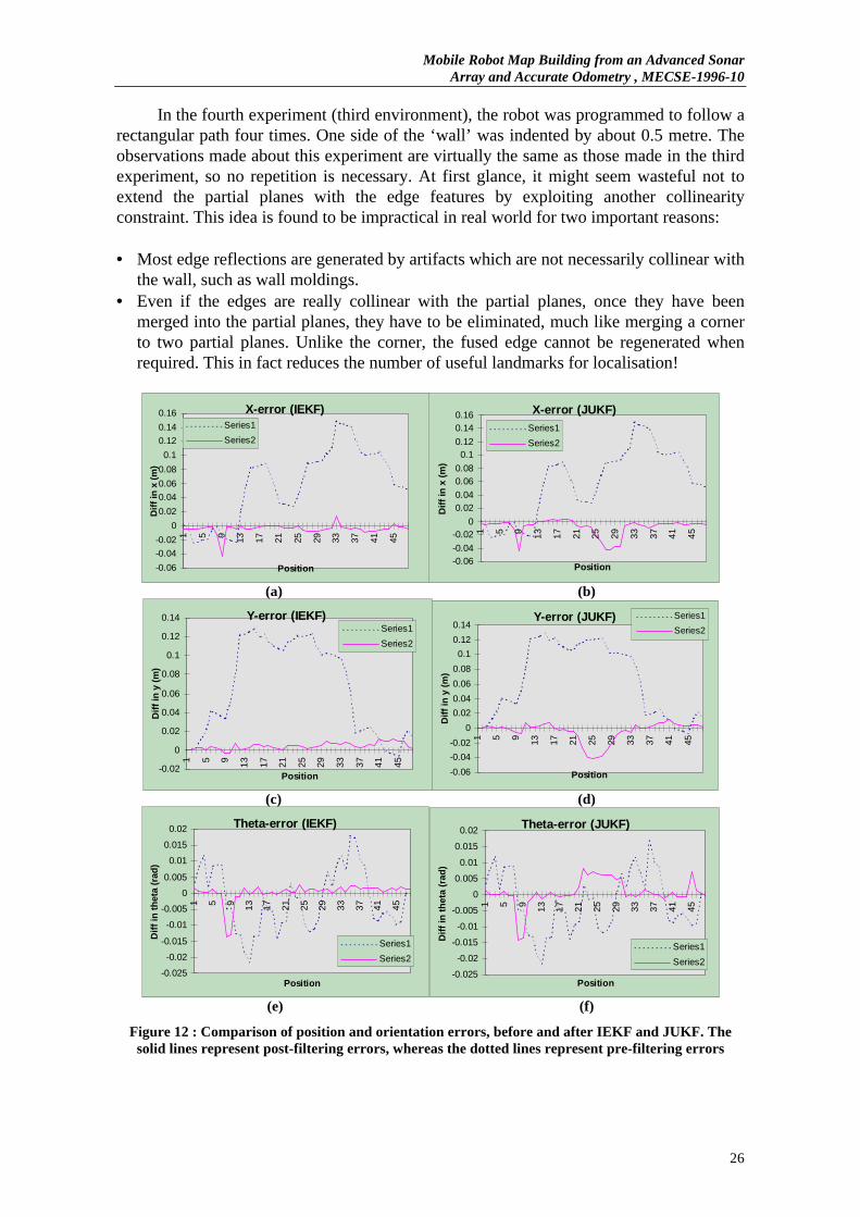
times to rescan the environment. The total distance travelled is 4×8×4=128 metres, andthe total number of scanning points is 4×12=48. The comparison of the pre-filteringposition errors and post-filtering position errors at all stops is show in Figure 12.

Both methods yield approximately the same performance, with JUKF showing more‘jitters’ at some scanning points. At the end of the second round, both IEKF simulationand JUKF simulation register a total of 9 partial planes, but at the end of the fourth round,the IEKF simulation registers a total of 13 partial planes whereas the JUKF simulationregisters a total of 18 partial planes. By single stepping the program, it has been confirmedthat the only reason for the appearance of redundant partial planes is the failure in passingthe χ2 test. The algorithms for growing map primitives have also been verified as workingcorrectly and satisfactorily.

Running on a SGI INDY and code compiled with GNU GCC 2.7.0, the speedrequired by JUKF to complete the simulation is approximately 5 times that required byIEKF.

7 Experimental Results

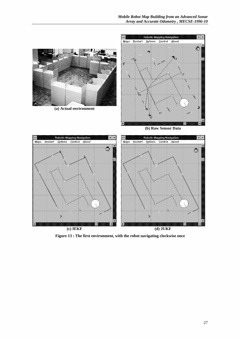
Experiments have been carried out in four artificial environment erected with cardboardboxes and they are shown from Figure 13(a) to Figure 16(a). The odometry of the robothas been calibrated to reduce systematic errors, and the parameters required by the non-systematic error model have been obtained in [3] prior to experiment.


25

Since the cardboard boxes were being lined up manually taking the gridlines on theparquetry floor as reference, the variance associated with the time of flight measurementand angular measurement were set larger than that achievable by the sonar sensor [8] inorder for the collinearity constraints to hold. The initial value of speed of sound was set to342.5 m/s, which is the mean value at the time. In fact, for all four experiments, thefollowing tentative values were used:

standard deviation of time of flight = 1.6×10-5 sstandard deviation of direction = 2.4°initial standard deviation of cs = 0.18 m/s

The resultant maps are shown in Figure 13(c)(d) to Figure 16(c)(d). The (b)subfigures show the raw sonar measurements detected at various positions (beforeposition correction) being superimposed onto the same diagrams, and the ‘scan lines’from one of the position indicate the typical number of features the sonar sensor cancapture at any one time. The grid spacing is 1 metre. It has been noticed that the sensordetects the gaps between the cardboard boxes as edges. They should not be regarded assome artificial aids to the mapping process as in a real environment, wall moldings areoften found to give rise to the same phenomenon.

In the first environment, the robot navigated around the enclosure once, firstclockwise (Figure 13) then counterclockwise (Figure 14). The maps generated with JUKFand IEKF are very similar except that for the clockwise experiment, IEKF does not mergethe two partial planes on the right which are supposed to belong to the same ‘wall’. Also,IEKF does not fuse several corners to the intersecting planes in both runs. Their fusion tothe planes are found to be hindered by the χ2 tests. A comparison of the covariancegenerated by IEKF and JUKF for a few features indicates that JUKF in general tends togenerate larger covariance. As a result, the error ellipses for ‘related’ features are morelikely to overlap and more mergence can be observed. Despite the minor imperfection, allpost-filtering maps show that only one partial plane is generated for each wall, and mostof the corners have been successfully fused to two intersecting partial planes, hence welldefined intersections can be observed. Also, repetitive observations of the same edge areall successfully merged into one edge map feature. All unterminated endpoints of partialplanes have also been properly projected to the line parameters. In the counterclockwiserun, a phantom target can be observed (refer to (b)) but it has been eliminated by itsneareast partial plane. Overall, the maps produced by IEKF and JUKF are very similar.

The third experiment (second environment) is more challenging. The robot wasprogrammed to repetitively enter, make a 180° turn, exit an enclosure four times toinvestigate the long term performance of both filters. Once again, both filters haveremained consistent throughout the navigation. JUKF produces a map with all featurescorrectly merged. IEKF’s performance closely matches that of JUKF, with only onecorner not fused to two partial planes and two edge features not identified as belonged tothe same physical edge. Three phantom corners are retained in the raw data map, but aresubsequently eliminated in the post-filtering maps by the partial planes blocking theirlines of sight. Once again, the maps produced by IEKF and JUKF are very similar, but thespeed of JUKF is significantly slower.


26

In the fourth experiment (third environment), the robot was programmed to follow arectangular path four times. One side of the ‘wall’ was indented by about 0.5 metre. Theobservations made about this experiment are virtually the same as those made in the thirdexperiment, so no repetition is necessary. At first glance, it might seem wasteful not toextend the partial planes with the edge features by exploiting another collinearityconstraint. This idea is found to be impractical in real world for two important reasons:

• Most edge reflections are generated by artifacts which are not necessarily collinear withthe wall, such as wall moldings.

• Even if the edges are really collinear with the partial planes, once they have beenmerged into the partial planes, they have to be eliminated, much like merging a cornerto two partial planes. Unlike the corner, the fused edge cannot be regenerated whenrequired. This in fact reduces the number of useful landmarks for localisation!

X-error (IEKF)

-0.06

-0.04

-0.02

0

0.02

0.04

0.06

0.08

0.1

0.12

0.14

0.16

1 5 9 13 17 21 25 29 33 37 41 45

Position

Dif

f in

x (

m)

Series1

Series2

X-error (JUKF)

-0.06-0.04

-0.020

0.020.040.060.08

0.10.12

0.140.16

1 5 9 13 17 21 25 29 33 37 41 45

Position

Dif

f in

x (

m)

Series1

Series2

(a) (b)

Y-error (IEKF)

-0.02

0

0.02

0.04

0.06

0.08

0.1

0.12

0.14

1 5 9 13 17 21 25 29 33 37 41 45

Position

Dif

f in

y (

m)

Series1

Series2

Y-error (JUKF)

-0.06

-0.04

-0.02

0

0.02

0.04

0.06

0.08

0.1

0.12

0.14

1 5 9 13 17 21 25 29 33 37 41 45

Position

Dif

f in

y (

m)

Series1

Series2

(c) (d)

Theta-error (IEKF)

-0.025

-0.02

-0.015

-0.01

-0.005

0

0.005

0.01

0.015

0.02

1 5 9 13 17 21 25 29 33 37 41 45

Position

Dif

f in

th

eta

(rad

)

Series1

Series2

Theta-error (JUKF)

-0.025

-0.02

-0.015

-0.01

-0.005

0

0.005

0.01

0.015

0.02

1 5 9 13 17 21 25 29 33 37 41 45

Position

Dif

f in

th

eta

(rad

)

Series1

Series2

(e) (f)

Figure 12 : Comparison of position and orientation errors, before and after IEKF and JUKF. Thesolid lines represent post-filtering errors, whereas the dotted lines represent pre-filtering errors


27

(a) Actual environment

(b) Raw Sensor Data

(c) IEKF (d) JUKF

Figure 13 : The first environment, with the robot navigating clockwise once


28


(b) Pre-filtering Perception

(e) IEKF (d) JUKF

Figure 14 : The first environment, with the robot navigating counterclockwise once


29



(e) IEKF (d) JUKF

Figure 15 : The second environment, with the robot navigating into and out of the enclosure fourtimes


30



(c) IEKF (d) JUKF

Figure 16 : The third environment, with the robot repeating a retangular path four times


31

8 Conclusion

The capability of autonomous navigation by mapping of our mobile robot system in somesimple environments has been demonstrated. IEKF and JUKF have been employed to dealwith the problem of covariance propagation through nonlinear transformation, and theirstrengths and weaknesses with regards to accuracy and speed have been compared withsimulated and real data. It has been shown that the accuracy demonstrated by IEKF iscomparable to that by JUKF and is in fact sufficient in practice. While eliminating thetedium of deriving Jacobian matrices, JUKF is less efficient compared to IEKF. Thealgorithm is now being intensively upgraded to enhance its robustness and efficiency.Current research focal points include the elimination of the storage and update of thecovariance between two features if it is found to be small, in order to improve the speedand memory requirement of the algorithm. Also under investigation is a map matchingstrategy to re-establish robot’s position when its uncertainty is too large or when theaccumulation of position bias becomes significant.

9 Acknowledgment

Mr. Greg Curmi’s assistance in the design of the robot and sonar implementation isgratefully acknowledged.


32

10 References

[1] Ayache, N. and Faugeras, O.D. "Maintaining Representation of the Environment of aMobile Robot", IEEE Transactions on Robotics and Automation, Vol 5, No 6, Dec1989, pp.804-819.

[2] Bar-Shalom, Y. and Li, X.R. "Estimation and Tracking: Principles, Techniques andsoftware", Boston, London: Artech House Inc., 1993.

[3] Chong, K.S. and Kleeman, L. “Accurate Odometry and Error Modelling for a MobileRobot”, to appear in Proceedings of the 1997 IEEE International Conference onRobotics and Automation.

[4] Dudek, G. et al “Just-in-time Sensing: Efficiently Combining Sonar and Laser RangeData for Exploring Unknown Worlds”, Proceedings 1996 IEEE InternationalConference on Robotics and Automation, pp.667-672.

[5] Durrant-Whyte, H.F. and Leonard, J.J. "Simultaneous Map Building and Localisationfor an Autonomous Robot", IEEE/RSJ International Workshop on Intelligent Robotsand Systems IROS '91, Nov 3-5, 1991, pp.1442-1447.

[6] Gonzalez, J. "An Iconic Position Estimator for a 2D Laser RangeFinder" Proceedings1992 IEEE International Conference on Robotics and Automation, Vol 3, pp.2646-2651.

[7] Hong, M.L. and Kleeman, L. "A Low Sample Rate 3D Sonar Sensor for MobileRobots", IEEE International Conference on Robotics and Automation, 1995, pp.3015-3020.

[8] Jazwinski, A.H. “Stochastic Processes and Filtering Theory”, New York: AcademicPress, 1970.

[9] Julier, S. and Uhlmann, J. "A General Method for Approximating NolinearTransformations of Probability Distributions", 1995, WWW.

[10] Kleeman, L. and Kuc, R. "Mobile Robot Sonar for Target Localization andClassification", The International Journal of Robotics Research, Vol. 14, No 4, August1995, pp.295-318.

[11] Kuc, R. and Siegel, M.W. "Physically Based Simulation Model for Acoustic SensorRobot Navigation", IEEE Transactions on Pattern Analysis and Machine Intelligence,Vol PAMI-9, No 6, Nov 1987, pp.766-778.

[12] Leonard, J.J. and Durrant-Whyte H.F. "Dynamic Map Building for an AutonomousMobile Robot", International Journal of Robotics Research, August 1992, Vol 11,pp.286-298.

[13] Lim, J.H. and Cho, D.W. "Experimental Investigation Of Mapping and NavigationBased on Certainty Grid Using Sonar Sensors", Robotica, Jan-Feb 1993, Vol 11,Iss:part 1, pp.7-17.

[14] Lu, F. and Milios, E.E. "Optimal Global Pose Estimation for Consistent Sensor DataRegistration", Proceedings 1995 IEEE International Conference on Robotics andAutomation, pp.93-100.

[15] Moutarlier, P. and Chatila, R. "Stochastic Multisensory Data Fusion for MobileRobot Location and Environment Modeling", 5th International Symposium onRobotics Research, Tokyo, 1989, pp.85-94.

[16] Moravec, H.P. and Elfes, A. "High Resolution Map From Wide-Angle Sonar",Proceedings 1985, IEEE International Conference on Robotics and Automation,pp.116-121.


33

[17] Neira, J. et al “Multisensor Mobile Robot Localisation” Proceedings 1996International Conference on Robotics and Automation, pp.673-679.

[18] Ohya, A. et al "Exploring Unknown Environment and Map Construction UsingUltrasonic Sensing of Normal Direction of Walls", pp.485-492.

[19] Oriolo, G. et al "On-Line Map Building and Navigation for Autonomous MobileRobots", IEEE International Conference on Robotics and Automation, 1995, pp.2900-2906.

[20] Pagac, D. et al “An Evidential Approach to Probabilistic Map-Building”,Proceedings 1996 IEEE International Conference on Robotics and Automation, pp.745-750.

[21] Rencken, W.D. "Concurrent Localisation and Map Building for Mobile Robots UsingUltrasonic Sensors", Proceedings 1993 IEEE International Conference On Roboticsand Automation, Vol 3, pp.2192-2197.

[22] Smith, R.C. and Cheeseman, P. "On the Representation and Estimation of SpatialUncertainty", The International Journal of Robotics Research, Vol 5, No 4, 1986,pp.56-68.

mobile robot map building from an advanced sonar...

Documents