mixing (mx) oceanographic toolbox for em-apex* ﬂoat data … · 2017-02-14 · mixing (mx)...

Institute

forMarine

andAntarcticStudies

MixingToolbox

Institute for Marine

and Antarctic Studies

University of Tasmania

IMAS Technical Report 2014/01

Mixing (MX) Oceanographic Toolbox for EM-APEX*float data applying shear-strain finescaleparameterization

* Electromagnetic Autonomous Profiling Explorer (EM-APEX)

Amelie Meyer, Helen E. Phillips, Bernadette M. Sloyanand Kurt L. Polzin

July 2014Revised September 2015

Dep

th (m

)

200

400

600

800

1000

1200

1400

log 10

(Kl) (

m2 s−

1 )

−6.5

−6

−5.5

−5

−4.5

−4

−3.5

−3

−2.5

Float Float Float Float Float Float Float Float3760 3761 3952 3950 3762 3951 4051 3764

Approved for public release; distribution is unlimited.

IMAS Technical Report 2014/01 Mixing Toolbox

July 2014

Revised September 2015

Mixing (MX) Oceanographic Toolbox forEM-APEX* float data applying shear-strainfinescale parameterization* Electromagnetic Autonomous Profiling Explorer (EM-APEX)

Amelie Meyer and Helen E. Phillips

Institute for Marine and Antarctic Studies, andARC Centre of Excellence for Climate System ScienceUniversity of Tasmania20 Castray EsplanadeBattery Point, Tasmania 7004

Bernadette M. Sloyan

CSIROOcean and Atmosphere FlagshipGPO Box 1538Hobart, Tasmania 7001

Kurt L. Polzin

Woods Hole Oceanographic InstitutionWoods Hole, Massachusetts

Final ReportApproved for public release; distribution is unlimited.

Funded by the ARC centre of Excellence for Climate SystemScience, the Quantitative Marine Science program at IMASand the 2009 CSIRO Wealth from Ocean Flagship CollaborativeFund Postgraduate Scholarship.

IMAS www.imas.utas.edu.au

Mixing Toolbox ii

Abstract: The Mixing Oceanographic Toolbox provides a framework to es-

timate the dissipation rate and di↵usivity from Electromagnetic Autonomous

Profiling Explorer (EM-APEX) float observational data. The EM-APEX

floats measure the temperature, salinity, pressure, and horizontal velocity of

the current. Vertical gradients of velocity and buoyancy are estimated and

a finescale parameterization is applied. This method provides order of mag-

nitude estimates of mixing as well as estimates of the regional variability of

mixing.

Reference: For bibliographic purposes, this document should be cited as follows:

Meyer, A., H. E. Phillips, B. M. Sloyan, and K. L. Polzin: Mixing (MX) Oceanographic Toolbox for EM-APEX* float dataapplying shear-strain finescale parameterization, 69pp, Inst. for Marine and Antarctic Studies, Hobart, Technical Report,August 2014.

ISBN: 978-1-86295-770-1

Mixing Toolbox iii

Table of Contents

List of Figures ......................................................................................... v

1 Introduction ...................................................................................... 1

1.1 Estimating mixing ................................................................................ 2

1.2 EM-APEX floats .................................................................................. 2

Float characteristics ..................................................................................... 2

2 Installing the Mixing (MX) Oceanographic Toolbox in Matlab ....................... 5

3 Overview of the Mixing (MX) Oceanographic Toolbox library ........................ 6

3.1 Structure of the MX Toolbox mixing analysis............................................... 6

3.1.1 Load and build the dataset ................................................................... 6

3.1.2 Derive the fall rate of the EM-APEX float ................................................ 6

3.1.3 Grid the data .................................................................................... 6

3.1.4 Derive initial variables.......................................................................... 6

3.1.5 Plot initial variables ............................................................................ 6

3.1.6 Derive mixing variables ........................................................................ 7

3.1.7 Derive mixing .................................................................................... 7

3.1.8 Plot mixing variables ........................................................................... 7

3.2 List of input parameters ......................................................................... 7

3.3 List of output variables .......................................................................... 9

3.4 List of functions and data files in the MX Toolbox ...................................... 10

4 Application to EM-APEX float data from the SOFine project ...................... 11

4.1 SOFine project .................................................................................. 11

4.2 Initial variables .................................................................................. 14

4.2.1 Temperature .................................................................................... 14

4.2.2 Salinity ........................................................................................... 14

4.2.3 Buoyancy frequency ........................................................................... 15

4.2.4 Mixed layer depth .............................................................................. 15

4.2.5 Current speed ................................................................................... 15

4.3 Mixing variables ................................................................................. 16

4.3.1 Dissipation rate................................................................................. 16

4.3.2 Di↵usivity ........................................................................................ 16

4.3.3 Ratio of rotary shear variance ............................................................... 17

4.3.4 Shear-to-strain ratio ........................................................................... 18

5 Acknowledgements............................................................................ 19

References ............................................................................................ 20

Appendix A: Symbols and Notations ........................................................... 23

Mixing Toolbox iv

Appendix B: Matlab code for the Mixing (MX) Oceanographic Toolbox ............... 24

B.1 Analysis ........................................................................................... 24

B.2 Load and build the dataset ................................................................... 27

B.2.1 mx build initial data.m ....................................................................... 27

B.3 Derive the fall rate of the EM-APEX float ................................................ 28

B.3.1 mx derive fallrate.m ........................................................................... 28

B.4 Grid the data .................................................................................... 29

B.4.1 mx grid initialdata.m .......................................................................... 29

B.5 Derive initial variables ......................................................................... 31

B.5.1 mx derive abs T S.m.......................................................................... 31

B.5.2 mx derive potential density anomaly.m.................................................... 32

B.5.3 mx derive N2.m ................................................................................ 32

B.5.4 mx derive mixed layer depth.m ............................................................. 33

B.5.5 mx derive current speed.m................................................................... 34

B.6 Plot initial variables ............................................................................ 35

B.6.1 mx grid all initial data.m ..................................................................... 35

B.6.2 mx plot temperature.m ....................................................................... 37

B.6.3 mx plot salinity.m .............................................................................. 38

B.6.4 mx plot mixed layer depth.m ................................................................ 39

B.6.5 mx plot current speed.m ..................................................................... 40

B.7 Derive mixing variables ........................................................................ 41

B.7.1 mx derive N2 ref.m ............................................................................ 41

B.7.2 mx derive N2 100m.m ........................................................................ 43

B.7.3 mx derive strain.m ............................................................................. 43

B.7.4 mx derive shear.m ............................................................................. 44

B.8 Derive mixing .................................................................................... 45

B.8.1 mx grid mixingdata.m......................................................................... 45

B.8.2 mx derive mixing.m............................................................................ 46

B.8.3 mx derive mixing shear.m .................................................................... 47

B.8.4 mx derive mixing strain.m ................................................................... 53

B.8.5 mx derive mixing shearstrain.m ............................................................. 57

B.9 Plot mixing variables ........................................................................... 59

B.9.1 mx plot dissipation rate.m ................................................................... 59

B.9.2 mx plot di↵usivity.m........................................................................... 60

B.9.3 mx plot CCW CW.m.......................................................................... 61

B.9.4 mx plot Rw.m .................................................................................. 62

B.10 Function to check the installation of the library .......................................... 63

B.10.1 mx check functions.m......................................................................... 63

Mixing Toolbox v

List of Figures

Figure 1. EM-APEX float prior to deployment in the wet lab. The cardboard box is used toprotect the float during the deployment procedure. Two characteristics specific to the EM-APEX float are the black fins allowing it to rotate as it sinks through the water column andthe grey electrodes close to the top of the float. ........................................................ 3

Figure 2. Cross-section of the EM-APEX electromagnetic subsystem at the level of the elec-trodes (Sandford 1978 [1] p191). ........................................................................... 4

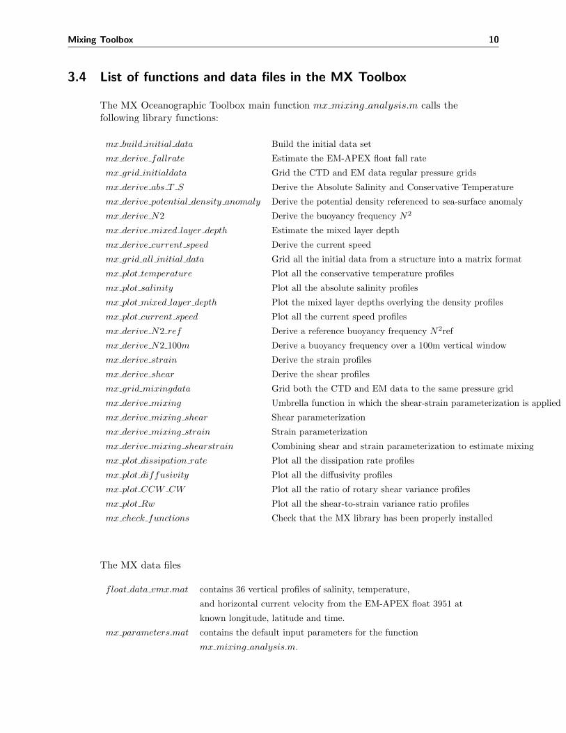
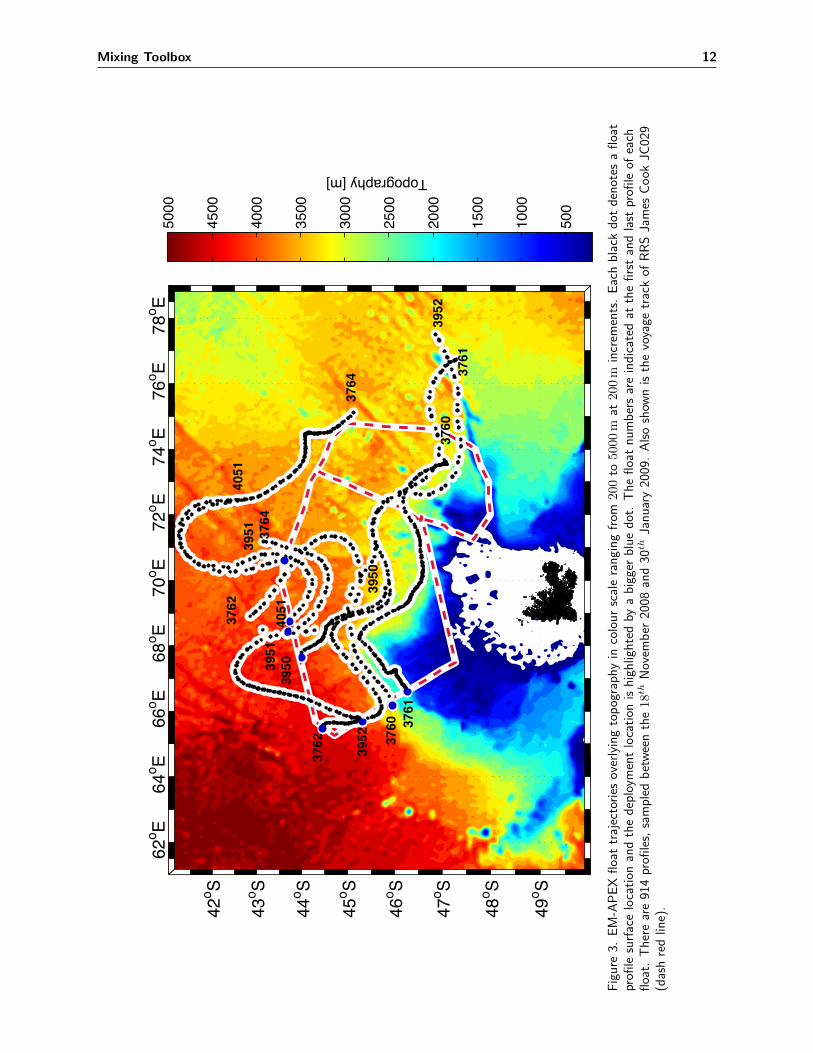
Figure 3. EM-APEX float trajectories overlying topography in colour scale ranging from 200to 5000m at 200m increments. Each black dot denotes a float profile surface location andthe deployment location is highlighted by a bigger blue dot. The float numbers are indicatedat the first and last profile of each float. There are 914 profiles, sampled between the 18th

November 2008 and 30th January 2009. Also shown is the voyage track of RRS James CookJC029 (dash red line)........................................................................................ 12

Figure 4. EM-APEX float vertical sampling strategy. The black line denotes the path of thefloat in the water column. The dotted line refers to profiles not used in this study. ........... 13

Figure 5. Vertical distribution of conservative temperature along the trajectory of float 3951.Potential density contours every 0.1 kgm�3 between �

✓

=27.0 and �✓

=29.0 kgm�3 areshown (grey) .................................................................................................. 14

Figure 6. Vertical distribution of absolute salinity along the trajectory of float 3951. Poten-tial density contours every 0.1 kgm�3 between �

✓

=27.0 and �✓

=29.0 kgm�3 are shown(grey) ........................................................................................................... 14

Figure 7. Vertical distribution of the squared buoyancy frequency N2 along the trajectoryof float 3951. Potential density contours every 0.1 kgm�3 between �

✓

=27.0 and �✓

=29.0kgm�3 are shown (grey) ................................................................................... 15

Figure 8. Mixed layer depth (black contour) overlying vertical distribution of potential den-sity along the trajectory of float 3951. ................................................................... 15

Figure 9. Vertical distribution of horizontal speed along the trajectory of float 3951. Poten-tial density contours every 0.1 kgm�3 between �

✓

=27.0 and �✓

=29.0 kgm�3 are shown(grey). .......................................................................................................... 16

Figure 10. Vertical distribution of the dissipation rate (✏) along the trajectory of float 3951.Potential density contours every 0.1 kgm�3 between �

✓

=27.0 and �✓

=29.0 kgm�3 areshown (grey). ................................................................................................. 16

Figure 11. Vertical distribution of di↵usivity (K⇢

) along the trajectory of float 3951. Poten-tial density contours every 0.1 kgm�3 between �

✓

=27.0 and �✓

=29.0 kgm�3 are shown(grey). .......................................................................................................... 17

Figure 12. Vertical distribution of the ratio of rotary shear variance (CCW/CW ) along thetrajectory of float 3951. Potential density contours every 0.1 kgm�3 between �

✓

=27.0 and�✓

=29.0 kgm�3 are shown (grey). ...................................................................... 17

Figure 13. Vertical distribution of the shear-to-strain ratio (R!

) along the trajectory of float3951. Potential density contours every 0.1 kgm�3 between �

✓

=27.0 and �✓

=29.0 kgm�3

are shown (grey).............................................................................................. 18

Mixing Toolbox vi

Mixing Toolbox 1

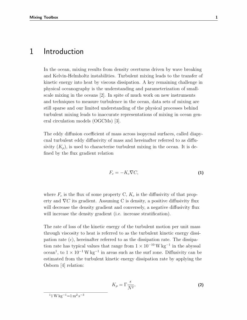
1 Introduction

In the ocean, mixing results from density overturns driven by wave breaking

and Kelvin-Helmholtz instabilities. Turbulent mixing leads to the transfer of

kinetic energy into heat by viscous dissipation. A key remaining challenge in

physical oceanography is the understanding and parameterization of small-

scale mixing in the oceans [2]. In spite of much work on new instruments

and techniques to measure turbulence in the ocean, data sets of mixing are

still sparse and our limited understanding of the physical processes behind

turbulent mixing leads to inaccurate representations of mixing in ocean gen-

eral circulation models (OGCMs) [3].

The eddy di↵usion coe�cient of mass across isopycnal surfaces, called diapy-

cnal turbulent eddy di↵usivity of mass and hereinafter referred to as di↵u-

sivity (K⇢), is used to characterise turbulent mixing in the ocean. It is de-

fined by the flux gradient relation

Fc = �KcrC, (1)

where Fc is the flux of some property C, Kc is the di↵usivity of that prop-

erty and rC its gradient. Assuming C is density, a positive di↵usivity flux

will decrease the density gradient and conversely, a negative di↵usivity flux

will increase the density gradient (i.e. increase stratification).

The rate of loss of the kinetic energy of the turbulent motion per unit mass

through viscosity to heat is referred to as the turbulent kinetic energy dissi-

pation rate (✏), hereinafter referred to as the dissipation rate. The dissipa-

tion rate has typical values that range from 1⇥ 10�10Wkg�1 in the abyssal

ocean1, to 1⇥ 10�1Wkg�1 in areas such as the surf zone. Di↵usivity can be

estimated from the turbulent kinetic energy dissipation rate by applying the

Osborn [4] relation:

K⇢ = �✏

N2, (2)

11Wkg�1=1m2 s�3

Mixing Toolbox 2

where the mixing e�ciency (� = 0.2) is assumed to be a constant. For fur-

ther details about the choice of �, see discussion in Polzin et al., (2014) [5].

1.1 Estimating mixing

Turbulence in the ocean is the result of a downscale energy cascade that

transfers energy and momentum from large scale currents towards smaller

scale internal waves, mostly as a result of nonlinear internal wave-wave inter-

actions [6]. Diapycnal mixing can be estimated directly as an area average

using tracer release experiments [7] or indirectly with microstructure profil-

ers (measuring shear with an air-foil shear probe) [8]. Diapycnal mixing can

also be indirectly estimated using finescale parameterization derived from

empirical and theoretical relations based on finescale observations of the in-

ternal wave field characteristic shear and strain. The intensity of turbulent

mixing is related to the energy and the shear of the local internal wave field

[9]. Many variants of the finescale parameterization exist using observations

of shear and strain, or either shear or strain only.

Finescale parameterization is based on (1) the assumption that most of the

turbulent mixing is driven by breaking internal waves (locally and remotely

generated) in the stratified ocean [10], and (2) the notion of a downscale en-

ergy cascade. The finescale parameterizations have been widely used in the

past decade [e.g. 11, 12, 13, 14, 15, 16, 17, 18, 19, 20], mostly because the

observations needed (profiles of vertical density and velocity) to derive the

dissipation rate with this method are much more easily acquired than direct

dissipation microstructure observations.

The uncertainties associated with these various finescale parameterization

methods are typically ±50% [21, 22, 5]. The method provides order of mag-

nitude estimates of mixing as well as estimates of the spatial gradients of

mixing.

1.2 EM-APEX floats

The EM-APEX is an innovative instrument that provides relatively inexpen-

sive, autonomous, high-resolution observations of velocity.

Float characteristics

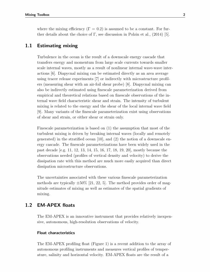
The EM-APEX profiling float (Figure 1) is a recent addition to the array of

autonomous profiling instruments and measures vertical profiles of temper-

ature, salinity and horizontal velocity. EM-APEX floats are the result of a

Mixing Toolbox 3

Figure 1. EM-APEX float prior to deployment in the wet lab. The cardboard box is used toprotect the float during the deployment procedure. Two characteristics specific to theEM-APEX float are the black fins allowing it to rotate as it sinks through the water columnand the grey electrodes close to the top of the float.

collaboration between the University of Washington Applied Physics Labo-

ratory (APL-UW) and Teledyne Webb Research Corporation (WRC). The

float combines a standard Teledyne APEX float with an electromagnetic

subsystem. The main technical characteristics of the EM-APEX float used

in this report are described below.

SBE-41 CTD

On the EM-APEX floats used in the SOFINE experiment, temperature (T),

salinity (S) and pressure (P) are measured by a Sea Bird Electronics SBE-

41 CTD. The float rate of descent and ascent has a range of 0.10 to 0.12

m s�1. The CTD is pumped on demand for approximately 2.5 s, delivering

40ml s�1 flow. The CTD sensor accuracy provided by the manufacturer is

2 dbar for pressure, 2⇥ 10�3 �C for temperature, and 2⇥ 10�3 for conductiv-

ity. The CTD data is processed in 2.2m vertical bins for preliminary anal-

ysis and then in 3m vertical bins when deriving mixing estimates to match

the electro-magnetic subsystem data vertical resolution (see below).

Mixing Toolbox 4

EM-APEX electromagnetic subsystem

The EM-APEX electromagnetic subsystem has a compass, accelerometer

and five electrodes to estimate the magnitude of horizontal currents (Fig-

ure 2). The horizontal velocity is estimated using the principle that a con-

ductor moving through a magnetic field develops an electrical potential drop

across the conductor. In this application, the conductor is seawater and the

magnetic field is that of the Earth [23]. The EM-APEX electromagnetic sub-

system voltmeter measures this electric potential di↵erence across the body

of the float with two independent pairs of electrodes.

Figure 2. Cross-section of the EM-APEX electromagnetic subsystem at the level of theelectrodes (Sandford 1978 [1] p191).

The float rotates with a period of 12 s due to external fins, and the motionally-

induced electric field is sampled at 20Hz and then averaged with a sinu-

soidal fit. The fit is made over 50 s long segments of data with 25 s between

successive fits, acting as a low-pass filter [24]. The fits provide an estimate

of the horizontal current and the residuals provide an estimate of the ve-

locity noise level at a vertical resolution of approximately 3m. Measured

voltages are transmitted over the Iridium global phone system and the pro-

cessing of the voltages into eastward and northward velocity components is

shore-based. The velocity profiles are relative to a depth-independent o↵set.

Given the GPS positions, by pairing profiles, the absolute velocity profile

can be estimated [25]. Profiles are gridded into 3m vertical bins for the mix-

ing analysis.

Mixing Toolbox 5

2 Installing the Mixing (MX) OceanographicToolbox in Matlab

Step 1

Download the MX Oceanographic Toolbox in Matlab from:www.mathworks.com.au/matlabcentral/fileexchange/47595-mixing–mx–oceanographic-toolbox-for-em-apex-float-data

Step 2

Create directory called ‘MX’ and unzip the Toolbox into this directory. Make surethat the two subfolders ‘figures’, and ‘private1’ have been extracted.

Step 3

In Matlab, add the ‘MX’ directory to your Matlab path using the option ‘Addwith subfolders...’. In the menu, go to ‘File’ or ’Home’, ‘Set Path...’, ‘Add withsubfolders...’. Make sure that the two subfolders ‘figures’, and ‘private1’ have beenadded to the path.

Step 4

From the MX directory, run mx check functions to check that the toolbox iscorrectly installed. Using the function as such applies a mixing finescale parame-terization to a set of 36 profiles from the EM-APEX float 3951. Figures from theanalysis are saved in the ‘MX’ directory under the folder ‘figures’.

Once the MX Oceanographic Toolbox is installed, you can run mx mixing analysis.mfor your own EM-APEX data. First you need to define the input data and param-eters. In matlab, type help mx mixing analysis.m to get a description of theinput parameters and what format the input data file needs to follow. Note thatyou will need the GSW Oceanographic Toolbox installed on your com-puter for the MX Oceanographic Toolbox to run. The GSW Oceano-graphic Toolbox can be downloaded from www.TEOS-10.org.

Mixing Toolbox 6

3 Overview of the Mixing (MX) OceanographicToolbox library

3.1 Structure of the MX Toolbox mixing analysis

A detailed descriptions of the theory and methods applied in this library can befound in Meyer et al. (2015) [26].

3.1.1 Load and build the dataset

In this section, we load the input data set of profiles from the EM-APEX floatand the parameters (‘mx parameters.mat’) that will be applied in the analysis.Next we extract the relevant data from the input data set and create a structure‘initial data.mat’.

3.1.2 Derive the fall rate of the EM-APEX float

In this short section, the fall rate of the EM-APEX float is estimated at each bindepth of each profile and added to the ‘initial data.mat’ structure.

3.1.3 Grid the data

Both the CTD data (temperature and salinity) and the EM data (velocity and fallrate) are gridded on a regular pressure grid using ‘mx grid initialdata.m’. Thisgrid is preset to vertical intervals of 2.2 dbar for the CTD data and 3 dbar for theEM data. These values can be changed manually in the code ‘mx grid initialdata.m’.The gridded data is saved in the same structure ‘initial data.mat’.

3.1.4 Derive initial variables

In this section, we derive some initial variables needed for the mixing calculations.First we evaluate Conservative Temperature (⇥) as a function of Absolute Salinity(SA), in situ temperature (T ) and pressure (P ) using the Gibbs Seawater Oceano-graphic Toolbox (GSW). Next we estimate the potential density (referenced to thesea surface) anomaly using the Gibbs Seawater Oceanographic Toolbox (GSW).We also estimate the buoyancy frequency (N), the mixed layer depth (MLD) andthe current speed (See (author?) [26] for derivation details). Each of these vari-ables are saved in ‘initial data.mat’.

3.1.5 Plot initial variables

Mixing Toolbox 7

The initial variables are changed from a structure file into a matrix ‘initial data gridded.mat’using ’mx grid all initial data.m’. The temperature, salinity, buoyancy frequency,mixed layer depth and current speed are then plotted and the figures are saved ina directory designated in the inputs.

3.1.6 Derive mixing variables

In this section, we derive some mixing variables needed for the mixing calcula-tions. First we evaluate a reference background buoyancy frequency (N2 ref).Next we estimate the buoyancy frequency on a 100 dbar vertical length scale (N2 100m).We also estimate the strain and the shear in each EM-APEX profile. Each ofthese variables are saved in a new structure ‘mixing data.mat’.

3.1.7 Derive mixing

All the mixing variables are gridded onto a standard 3 dbar grid (‘mx grid mixingdata.m’)and saved into a new structure ‘mixing data gridded.mat’. The shear-strain finescaleparameterization is applied (‘mx derive mixing.m’) and the dissipation rate (✏)and di↵usivity (K⇢) estimated. The mixing data is saved in a new structure ‘mix-ing data gridded run.mat’.

3.1.8 Plot mixing variables

The dissipation rate (✏), di↵usivity (K⇢), ratio of CCW to CW rotating shearvariance (�CCW /�CW ) and Shear-to-strain variance ratio (R!) are plotted. Thefigures are saved in a directory designated in the inputs.

3.2 List of input parameters

U = ‘10; U velocity sensor: can be either ‘1’ or ‘2’

V = ‘10; V velocity sensor: can be either ‘1’ or ‘2’

moving window = 20; Number of consecutive profiles used to estimate N2 ref.

dzN2ref = 24; Vertical number of bin depth used to estimate N2 ref.

dzN2 = 6; Di↵erential length for N2 calculation: e.g. 6 (m).

drho = 0.03; Density gradient to derive the mixed layer depth: 0.03 kgm�4

dz = 3; Main data set pressure grid interval (m).

dzs = 6; Vertical scale over which shear is derived. Must be a multiple

of dz.

fftpt = 128; Number of points for the fast fourier transform e.g.

128 but could be 32,64,128... or any power of 2.

lzmin fixed = 50; Minimum wavelength integration for shear/strain spectra (m).

lzmax fixed = 300; Maximum wavelength integration for shear/strain spectra (m).

Constants:

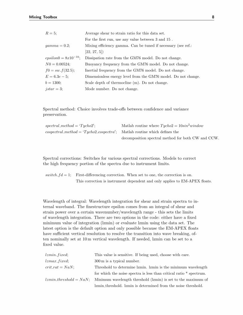
Mixing Toolbox 8

R = 5; Average shear to strain ratio for this data set.

For the first run, use any value between 3 and 15 .

gamma = 0.2; Mixing e�ciency gamma. Can be tuned if necessary (see ref.:

[22, 27, 5])

epsilon0 = 8x10�10; Dissipation rate from the GM76 model. Do not change.

N0 = 0.00524; Buoyancy frequency from the GM76 model. Do not change.

f0 = sw f(32.5); Inertial frequency from the GM76 model. Do not change.

E = 6.3e� 5; Dimensionless energy level from the GM76 model. Do not change.

b = 1300; Scale depth of thermocline (m). Do not change.

jstar = 3; Mode number. Do not change.

Spectral method: Choice involves trade-o↵s between confidence and variancepreservation.

spectral method = ‘Tycho20; Matlab routine where Tycho2 = 10sin2window

cospectral method = ‘Tycho2 cospectra0; Matlab routine which defines the

decomposition spectral method for both CW and CCW.

Spectral corrections: Switches for various spectral corrections. Models to correctthe high frequency portion of the spectra due to instrument limits.

switch fd = 1; First-di↵erencing correction. When set to one, the correction is on.

This correction is instrument dependent and only applies to EM-APEX floats.

Wavelength of integral: Wavelength integration for shear and strain spectra to in-ternal waveband. The finestructure epsilon comes from an integral of shear andstrain power over a certain wavenumber/wavelength range - this sets the limitsof wavelength integration. There are two options in the code: either have a fixedminimum value of integration (lzmin) or evaluate lzmin using the data set. Thelatest option is the default option and only possible because the EM-APEX floatshave su�cient vertical resolution to resolve the transition into wave breaking, of-ten nominally set at 10m vertical wavelength. If needed, lzmin can be set to afixed value.

lzmin fixed; This value is sensitive. If being used, choose with care.

lzmax fixed; 300m is a typical number.

crit rat = NaN ; Threshold to determine lzmin. lzmin is the minimum wavelength

for which the noise spectra is less than critical ratio * spectrum.

lzmin threshold = NaN ; Minimum wavelength threshold (lzmin) is set to the maximum of

lzmin threshold. lzmin is determined from the noise threshold.

Mixing Toolbox 9

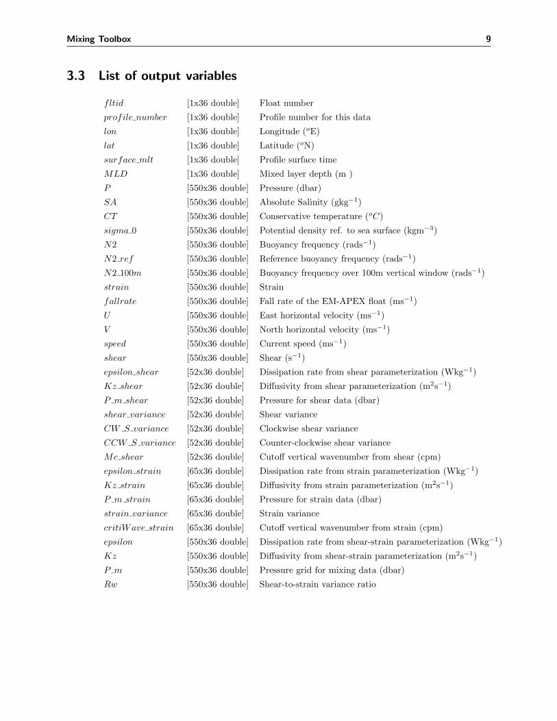
3.3 List of output variables

fltid [1x36 double] Float number

profile number [1x36 double] Profile number for this data

lon [1x36 double] Longitude (oE)

lat [1x36 double] Latitude (oN)

surface mlt [1x36 double] Profile surface time

MLD [1x36 double] Mixed layer depth (m )

P [550x36 double] Pressure (dbar)

SA [550x36 double] Absolute Salinity (gkg�1)

CT [550x36 double] Conservative temperature (oC)

sigma 0 [550x36 double] Potential density ref. to sea surface (kgm�3)

N2 [550x36 double] Buoyancy frequency (rads�1)

N2 ref [550x36 double] Reference buoyancy frequency (rads�1)

N2 100m [550x36 double] Buoyancy frequency over 100m vertical window (rads�1)

strain [550x36 double] Strain

fallrate [550x36 double] Fall rate of the EM-APEX float (ms�1)

U [550x36 double] East horizontal velocity (ms�1)

V [550x36 double] North horizontal velocity (ms�1)

speed [550x36 double] Current speed (ms�1)

shear [550x36 double] Shear (s�1)

epsilon shear [52x36 double] Dissipation rate from shear parameterization (Wkg�1)

Kz shear [52x36 double] Di↵usivity from shear parameterization (m2s�1)

P m shear [52x36 double] Pressure for shear data (dbar)

shear variance [52x36 double] Shear variance

CW S variance [52x36 double] Clockwise shear variance

CCW S variance [52x36 double] Counter-clockwise shear variance

Mc shear [52x36 double] Cuto↵ vertical wavenumber from shear (cpm)

epsilon strain [65x36 double] Dissipation rate from strain parameterization (Wkg�1)

Kz strain [65x36 double] Di↵usivity from strain parameterization (m2s�1)

P m strain [65x36 double] Pressure for strain data (dbar)

strain variance [65x36 double] Strain variance

critiWave strain [65x36 double] Cuto↵ vertical wavenumber from strain (cpm)

epsilon [550x36 double] Dissipation rate from shear-strain parameterization (Wkg�1)

Kz [550x36 double] Di↵usivity from shear-strain parameterization (m2s�1)

P m [550x36 double] Pressure grid for mixing data (dbar)

Rw [550x36 double] Shear-to-strain variance ratio

Mixing Toolbox 10

3.4 List of functions and data files in the MX Toolbox

The MX Oceanographic Toolbox main function mx mixing analysis.m calls thefollowing library functions:

mx build initial data Build the initial data set

mx derive fallrate Estimate the EM-APEX float fall rate

mx grid initialdata Grid the CTD and EM data regular pressure grids

mx derive abs T S Derive the Absolute Salinity and Conservative Temperature

mx derive potential density anomaly Derive the potential density referenced to sea-surface anomaly

mx derive N2 Derive the buoyancy frequency N2

mx derive mixed layer depth Estimate the mixed layer depth

mx derive current speed Derive the current speed

mx grid all initial data Grid all the initial data from a structure into a matrix format

mx plot temperature Plot all the conservative temperature profiles

mx plot salinity Plot all the absolute salinity profiles

mx plot mixed layer depth Plot the mixed layer depths overlying the density profiles

mx plot current speed Plot all the current speed profiles

mx derive N2 ref Derive a reference buoyancy frequency N2ref

mx derive N2 100m Derive a buoyancy frequency over a 100m vertical window

mx derive strain Derive the strain profiles

mx derive shear Derive the shear profiles

mx grid mixingdata Grid both the CTD and EM data to the same pressure grid

mx derive mixing Umbrella function in which the shear-strain parameterization is applied

mx derive mixing shear Shear parameterization

mx derive mixing strain Strain parameterization

mx derive mixing shearstrain Combining shear and strain parameterization to estimate mixing

mx plot dissipation rate Plot all the dissipation rate profiles

mx plot diffusivity Plot all the di↵usivity profiles

mx plot CCW CW Plot all the ratio of rotary shear variance profiles

mx plot Rw Plot all the shear-to-strain variance ratio profiles

mx check functions Check that the MX library has been properly installed

The MX data files

float data vmx.mat contains 36 vertical profiles of salinity, temperature,

and horizontal current velocity from the EM-APEX float 3951 at

known longitude, latitude and time.

mx parameters.mat contains the default input parameters for the function

mx mixing analysis.m.

Mixing Toolbox 11

4 Application to EM-APEX float data from theSOFine project

4.1 SOFine project

Eight EM-APEX floats were deployed during the RRS James Cook cruise JC029in late 2008 as part of the Southern Ocean FINEstructure (SOFine) project. TheSOFine project is a U.K., U.S. and Australian collaborative experiment to investi-gate the impact of finescale processes on the momentum balance in the AntarcticCircumpolar Current [28]. The floats were deployed on the northern edge of theKerguelen Plateau in late 2008 to drift along the Antarctic Circumpolar Current(ACC) (Figure 3).

While drifting north of the Kerguelen Plateau, the floats were programmed tosurface twice a day, measuring four profiles of temperature, salinity, pressure andhorizontal velocity from the sea surface to 1600m, with a parked drift of 8 hoursat 1000m (Figure 4). The floats spent typically 30minutes at the surface to trans-mit the profile data over the Iridium satellite network as opposed to floats trans-mitting over the Argos communication system spending on average 10 hours at thesurface. Using the Iridium communication system allows for two-way communi-cation as well as faster data transfer and therefore the option to sample at higherresolution. The floats only sampled the top 1600m of the water column ratherthan going to their maximum 2000m so that consecutive up profiles are approxi-mately half an inertial period apart (17 hours at 45� S latitude), and consequentlythe inertial frequency can be resolved in the data.

Mixing Toolbox 12

6

2o E 6

4o E 6

6o E 6

8o E 7

0o E 7

2o E 7

4o E 7

6o E 7

8o E

49o S

48o S

47o S

46o S

45o S

44o S

43o S

42o S

Topography [m]

500

1000

1500

2000

2500

3000

3500

4000

4500

5000

Amel

ie M

− 2

4−Ju

n−20

13EM

−APE

X da

taIn

itial

ana

lysi

s

3760

3760

3761

3761

3762

3762

3764

3764

3950

3950

3951

3951

3952

3952

4051

4051

Figure3.

EM-APEXfloattrajectories

overlyingtopograph

yin

colour

scalerang

ingfrom

200to

5000

mat

200m

increm

ents.Eachblackdo

tdeno

tesafloat

profi

lesurfacelocation

andthedeploymentlocation

ishigh

lighted

byabigger

blue

dot.

The

floatnu

mbersareindicatedat

thefirstandlast

profi

leof

each

float.

There

are914profi

les,sampled

betweenthe18

th

Novem

ber

2008

and30

th

Janu

ary2009.Alsoshow

nisthevoyage

trackof

RRSJames

Coo

kJC

029

(dashredline).

Mixing Toolbox 13

The cruise track with the deployment positions of the floats is shown in Figure 3.Five of the eight EM-APEX floats were deployed at a CTD station, allowing cal-ibration of the float salinity sensor with the CTD salinity observations. The datatransmitted by the floats over the Iridium phone system were received by a dataserver at the University of Tasmania and converted to relative velocity using soft-ware developed by John Dunlap at the University of Washington in the researchgroup of Prof. Tom Sanford. This was followed by extensive processing to cali-brate the instruments, automate the quality control of the velocity data, and toconvert relative velocity to absolute velocity [25].

!"#$%"

!"#$%"

&'"#$%"

()))"*"

&'"#$%" &'"#$%"

(+))"*"

Figure 4. EM-APEX float vertical sampling strategy. The black line denotes the path of thefloat in the water column. The dotted line refers to profiles not used in this study.

Mixing Toolbox 14

4.2 Initial variables

A detailed description of the methods and results can be found in Meyer et al.(2015) [26].

4.2.1 Temperature

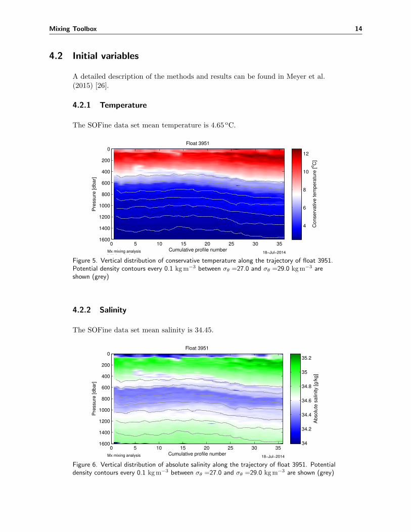
The SOFine data set mean temperature is 4.65 oC.

Cumulative profile number

Pre

ssure

[dbar]

Float 3951

0 5 10 15 20 25 30 35

0

200

400

600

800

1000

1200

1400

1600

Conse

rvativ

e tem

pera

ture

[oC

]

4

6

8

10

12

18−Jul−2014Mx mixing analysisInitial analysis

Figure 5. Vertical distribution of conservative temperature along the trajectory of float 3951.Potential density contours every 0.1 kgm�3 between �

✓

=27.0 and �✓

=29.0 kgm�3 areshown (grey)

4.2.2 Salinity

The SOFine data set mean salinity is 34.45.


Pre

ssure

[dbar]

Float 3951

0 5 10 15 20 25 30 35

0

200

400

600

800

1000

1200

1400

1600

Abso

lute

salin

ity [g/k

g]

34

34.2

34.4

34.6

34.8

35

35.2

18−Jul−2014Mx mixing analysis

Figure 6. Vertical distribution of absolute salinity along the trajectory of float 3951. Potentialdensity contours every 0.1 kgm�3 between �

✓

=27.0 and �✓

=29.0 kgm�3 are shown (grey)

Mixing Toolbox 15

4.2.3 Buoyancy frequency

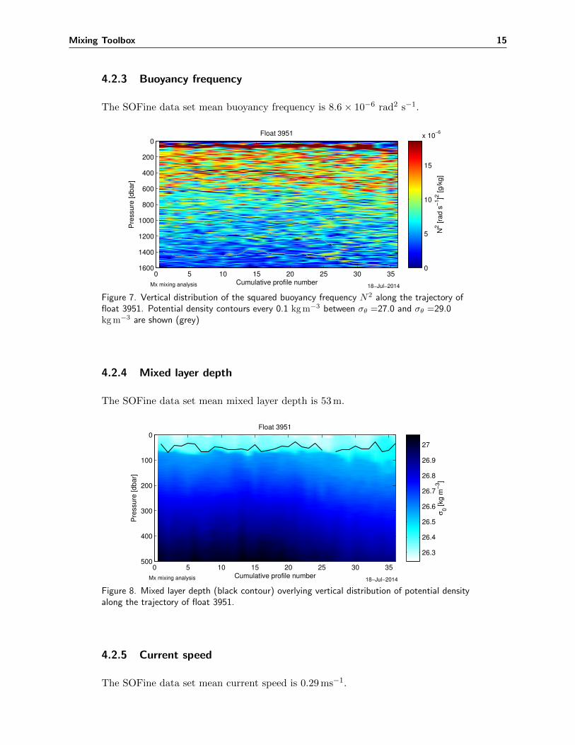
The SOFine data set mean buoyancy frequency is 8.6⇥ 10�6 rad2 s�1.


Pre

ssure

[dbar]

Float 3951

0 5 10 15 20 25 30 35

0

200

400

600

800

1000

1200

1400

1600

N2 [ra

d s

−1]2

[g/k

g]

0

5

10

15

x 10−6


Figure 7. Vertical distribution of the squared buoyancy frequency N2 along the trajectory offloat 3951. Potential density contours every 0.1 kgm�3 between �

✓

=27.0 and �✓

=29.0kgm�3 are shown (grey)

4.2.4 Mixed layer depth

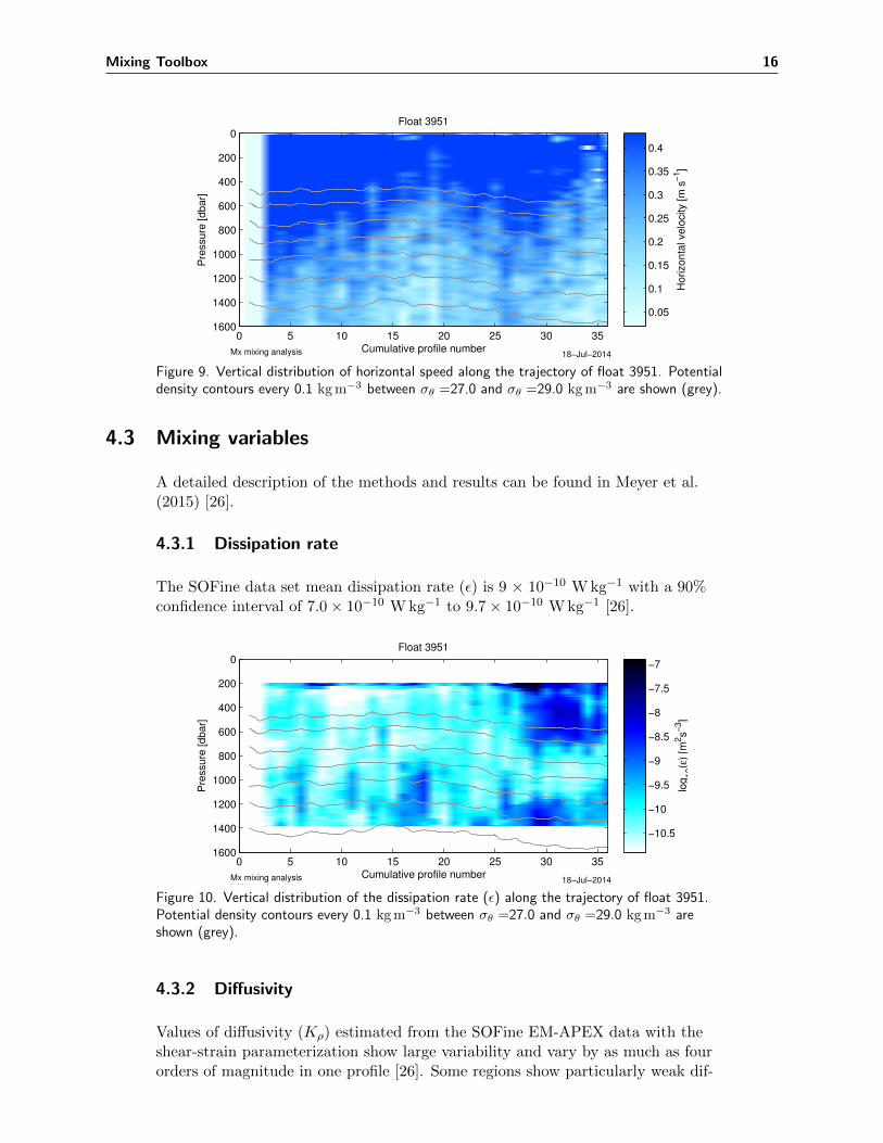
The SOFine data set mean mixed layer depth is 53m.


Pre

ssu

re [

db

ar]

Float 3951

0 5 10 15 20 25 30 35

0

100

200

300

400

500

σ0 [

kg m

−3]

26.3

26.4

26.5

26.6

26.7

26.8

26.9

27


Figure 8. Mixed layer depth (black contour) overlying vertical distribution of potential densityalong the trajectory of float 3951.

4.2.5 Current speed

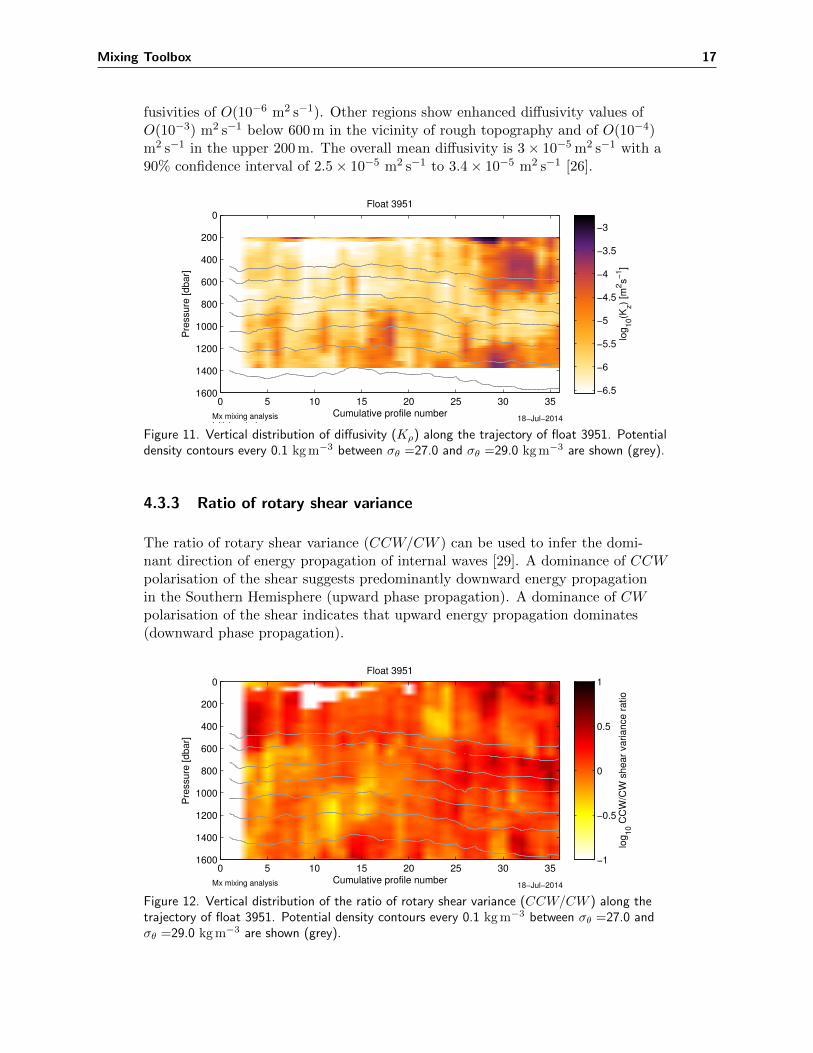
The SOFine data set mean current speed is 0.29ms�1.

Mixing Toolbox 16


Pre

ssure

[dbar]

Float 3951

0 5 10 15 20 25 30 35

0

200

400

600

800

1000

1200

1400

1600

Horizo

nta

l velo

city

[m

s−

1]

0.05

0.1

0.15

0.2

0.25

0.3

0.35

0.4


Figure 9. Vertical distribution of horizontal speed along the trajectory of float 3951. Potentialdensity contours every 0.1 kgm�3 between �

✓

=27.0 and �✓

=29.0 kgm�3 are shown (grey).

4.3 Mixing variables

A detailed description of the methods and results can be found in Meyer et al.(2015) [26].

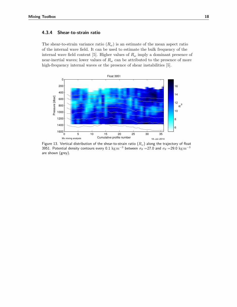
4.3.1 Dissipation rate

The SOFine data set mean dissipation rate (✏) is 9 ⇥ 10�10 Wkg�1 with a 90%confidence interval of 7.0⇥ 10�10 Wkg�1 to 9.7⇥ 10�10 Wkg�1 [26].


Pre

ssure

[dbar]

Float 3951

0 5 10 15 20 25 30 35

0

200

400

600

800

1000

1200

1400

1600

log

10(ε

) [m

2s−

3]

−10.5

−10

−9.5

−9

−8.5

−8

−7.5

−7


Figure 10. Vertical distribution of the dissipation rate (✏) along the trajectory of float 3951.Potential density contours every 0.1 kgm�3 between �

✓

=27.0 and �✓

=29.0 kgm�3 areshown (grey).

4.3.2 Di↵usivity

Values of di↵usivity (K⇢) estimated from the SOFine EM-APEX data with theshear-strain parameterization show large variability and vary by as much as fourorders of magnitude in one profile [26]. Some regions show particularly weak dif-

Mixing Toolbox 17

fusivities of O(10�6 m2 s�1). Other regions show enhanced di↵usivity values ofO(10�3) m2 s�1 below 600m in the vicinity of rough topography and of O(10�4)m2 s�1 in the upper 200m. The overall mean di↵usivity is 3⇥ 10�5m2 s�1 with a90% confidence interval of 2.5⇥ 10�5 m2 s�1 to 3.4⇥ 10�5 m2 s�1 [26].


Pre

ssure

[dbar]

Float 3951

0 5 10 15 20 25 30 35

0

200

400

600

800

1000

1200

1400

1600

log

10(K

z) [m

2s−

1]

−6.5

−6

−5.5

−5

−4.5

−4

−3.5

−3


Figure 11. Vertical distribution of di↵usivity (K⇢

) along the trajectory of float 3951. Potentialdensity contours every 0.1 kgm�3 between �

✓

=27.0 and �✓


4.3.3 Ratio of rotary shear variance

The ratio of rotary shear variance (CCW/CW ) can be used to infer the domi-nant direction of energy propagation of internal waves [29]. A dominance of CCWpolarisation of the shear suggests predominantly downward energy propagationin the Southern Hemisphere (upward phase propagation). A dominance of CWpolarisation of the shear indicates that upward energy propagation dominates(downward phase propagation).


Pre

ssure

[dbar]

Float 3951

0 5 10 15 20 25 30 35

0

200

400

600

800

1000

1200

1400

1600

log

10 C

CW

/CW

shear

variance

ratio

−1

−0.5

0

0.5

1


Figure 12. Vertical distribution of the ratio of rotary shear variance (CCW/CW ) along thetrajectory of float 3951. Potential density contours every 0.1 kgm�3 between �

✓

=27.0 and�✓


Mixing Toolbox 18

4.3.4 Shear-to-strain ratio

The shear-to-strain variance ratio (R!) is an estimate of the mean aspect ratioof the internal wave field. It can be used to estimate the bulk frequency of theinternal wave field content [5]. Higher values of R! imply a dominant presence ofnear-inertial waves; lower values of R! can be attributed to the presence of morehigh-frequency internal waves or the presence of shear instabilities [5].


Pre

ssu

re [

db

ar]

Float 3951

0 5 10 15 20 25 30 35

0

200

400

600

800

1000

1200

1400

1600

Rω

6

8

10

12

14

16


Figure 13. Vertical distribution of the shear-to-strain ratio (R!

) along the trajectory of float3951. Potential density contours every 0.1 kgm�3 between �

✓

=27.0 and �✓

=29.0 kgm�3

are shown (grey).

Mixing Toolbox 19

5 Acknowledgements

We thank Alberto Naveira Gabarato and Stephanie Waterman for their valuableguidance and contributions; John Dunlap for his valuable support during the datacollection and quality control stages of the project. We also thank Paul Barkerfor all his useful advice in creating and coding a matlab library. AM was sup-ported by the ARC centre of Excellence for Climate System Science, the Quanti-tative Marine Science program at IMAS, and the 2009 CSIRO Wealth from OceanFlagship Collaborative Fund Postgraduate Scholarship. HP is funded by the Aus-tralian Research Council Discovery Project (DP130102088). KLPs salary supportwas provided by Woods Hole Oceanographic Institution bridge support funds.Funding for the EM-APEX experiment was provided by the Australian ResearchCouncil Discovery Project (DP0877098) and Australian Government DEWHAProjects 3002 and 3228.

Mixing Toolbox 20

References

[1] T B Sanford, R G Drever, and J H Dunlap. A velocity profiler based on the princi-ples of geomagnetic induction. Deep-Sea Research, 25(2):183–210, 1978.

[2] M H Alford, M C Gregg, V Zervakis, and H Kontoyiannis. Internal wave measure-ments on the Cycladic Plateau of the Aegean Sea. Journal of Geophysical Research,117:C01015, 2012.

[3] Carl Wunsch and Ra↵aele Ferrari. Vertical Mixing, Energy, and the General Cir-culation of the Oceans. Annual Review of Fluid Mechanics, 36(1):281–314, January2004.

[4] T R Osborn. Estimates of the local-rate of vertical di↵usion from dissipation mea-surements. Journal of Physical Oceanography, 10(1):83–89, 1980.

[5] K L Polzin, A C Naveira Garabato, T N Huussen, B M Sloyan, and S N Waterman.Finescale parameterizations of turbulent dissipation. Journal of Geophysical Research- Oceans, 119:1383–1419, 2014.

[6] C H McComas and P Muller. The dynamic balance of internal waves. Journal ofPhysical Oceanography, 11(7):970–986, 1981.

[7] J. R. Ledwell, L. C. St. Laurent, J. B. Girton, J. M. Toole, L C St Laurent, J. B.Girton, and J. M. Toole. Diapycnal Mixing in the Antarctic Circumpolar Current.Journal of Physical Oceanography, 41(1):241–246, January 2011.

[8] M C Gregg. Diapycnal mixing in the thermocline - A review. Journal of GeophysicalResearch, 92(C5):5249–5286, 1987.

[9] K L Polzin, J M Toole, and R W Schmitt. Finescale parameterizations of turbulentdissipation. Journal of Physical Oceanography, 25(3):306–328, 1995.

[10] Matthew H Alford and Michael C Gregg. Near-inertial mixing: Modulation ofshear, strain and microstructure at low latitude. Journal of Geophysical Research,106(C8):16,916–947,968, 2001.

[11] C. Mauritzen, K L Polzin, M S McCartney, R C Millard, and D E West-Mack. Ev-idence in hydrography and density fine structure for enhanced vertical mixing overthe Mid-Atlantic Ridge in the western Atlantic. Journal of Geophysical Research,107(C10):11–19, 2002.

[12] A C Naveira Garabato, K L Polzin, B A King, K J Heywood, and M Visbeck.Widespread intense turbulent mixing in the Southern Ocean. Science, 303(5655):210–213, 2004.

[13] B. M. Sloyan. Spatial variability of mixing in the Southern Ocean. GeophysicalResearch Letters, 32(L18603):n/a–n/a, September 2005.

[14] E Kunze, E Firing, J M Hummon, T K Chereskin, A M Thurnherr, Ocean Sciences,British Columbia, San Diego, La Jolla, and Lamont-doherty Earth Observatory.

Mixing Toolbox 21

Global abyssal mixing inferred from lowered ADCP shear and CTD strain profiles.Journal of Physical Oceanography, 36(12):2350–2352, 2006.

[15] M. H. Alford, J. a. MacKinnon, Zhongxiang Zhao, Rob Pinkel, Jody M Klymak, andThomas Peacock. Internal waves across the Pacific. Geophysical Research Letters,34(24):L24601, December 2007.

[16] Young-Hyang H Park, Jean-Luc L Fuda, Isabelle Durand, Alberto C. Naveira Gara-bato, and A C N Garabato. Internal tides and vertical mixing over the KerguelenPlateau. Deep-Sea Research Part II-Topical Studies in Oceanography, 55(5-7):582–593, March 2008.

[17] Ilker Fer, Ragnheid Skogseth, and Florian Geyer. Internal Waves and Mixing in theMarginal Ice Zone near the Yermak Plateau. Journal of Physical Oceanography,40(7):1613–1630, July 2010.

[18] J A MacKinnon, M H Alford, R Pinkel, J Klymak, and Z Zhao. Mixing across thePacific. Journal of Physical Oceanography, 2011.

[19] Lixin Wu, Zhao Jing, Steve Riser, and Martin Visbeck. Seasonal and spatial varia-tions of Southern Ocean diapycnal mixing from Argo profiling floats. Nature Geo-science, 4(6):363–366, June 2011.

[20] C. B. Whalen, L. D. Talley, and J. a. MacKinnon. Spatial and temporal variabilityof global ocean mixing inferred from Argo profiles. Geophysical Research Letters,39(18):L18612, September 2012.

[21] K Polzin, E Kunze, J Hummon, and E Firing. The finescale response of loweredADCP velocity profiles. Journal of Atmospheric and Oceanic Technology, 19(2):205–224, 2002.

[22] S A Thorpe. The Turbulent Ocean. Number 439p. Cambridge University Press, 2005.

[23] T B Sanford, J H Dunlap, J A Carlson, D C Webb, and J B Girton. Autonomous ve-locity and density profiler: EM-APEX. Proceedings of the IEEE/OES eighth workingconference on current measurement technology - Proceedings, pages 152–156, 2005.

[24] Thomas B. Sanford, James F. Price, and James B. Girton. Upper-Ocean Responseto Hurricane Frances (2004) Observed by Profiling EM-APEX Floats. Journal ofPhysical Oceanography, 41(6):1041–1056, June 2011.

[25] H E Phillips and N L Bindo↵. On the non-Equivalent Barotropic structure of theAntarctic Circumpolar Current: An observational perspective. Journal of Geophysi-cal Research, 119:doi:10.1002/2013JC009516, 2014.

[26] A Meyer, B M Sloyan, K L Polzin, H E Phillips, and N L Bindo↵. Mixing variabilityin the Southern Ocean. Journal of Physical Oceanography, 45:966–987, 2015.

[27] G.N. N Ivey, K.B. B Winters, and J.R. R Kose↵. Density stratification, turbulence,but how much mixing? Annual Review of Fluid Mechanics, 40(1):169–184, January2008.

[28] A C Naveira Garabato. RRS James Cook Cruise 29, 01 Nov-22 Dec 2008. SOFineCruise Report: Southern Ocean Finestructure. Southampton Cruise Report 35, Na-tional Oceanography Centre, 2009.

Mixing Toolbox 22

[29] K D Leaman and T B Sanford. Vertical energy propagation of internal waves- Vector spectral analysis of velocity profiles. Journal of Geophysical Research,80(15):1975–1978, 1975.

Mixing Toolbox 23

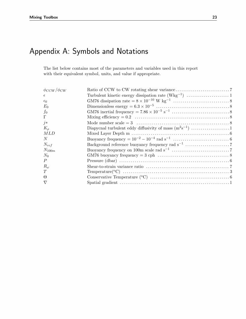
Appendix A: Symbols and Notations

The list below contains most of the parameters and variables used in this reportwith their equivalent symbol, units, and value if appropriate.

�CCW /�CW Ratio of CCW to CW rotating shear variance . . . . . . . . . . . . . . . . . . . . . . . . . . . . 7✏ Turbulent kinetic energy dissipation rate (Wkg�1) . . . . . . . . . . . . . . . . . . . . . . 1✏0 GM76 dissipation rate = 8⇥ 10�10 W kg�1 . . . . . . . . . . . . . . . . . . . . . . . . . . . . . 8E0 Dimensionless energy = 6.3⇥ 10�5 . . . . . . . . . . . . . . . . . . . . . . . . . . . . . . . . . . . . . . 8f0 GM76 inertial frequency = 7.86⇥ 10�5 s�1 . . . . . . . . . . . . . . . . . . . . . . . . . . . . . . 8� Mixing e�ciency = 0.2 . . . . . . . . . . . . . . . . . . . . . . . . . . . . . . . . . . . . . . . . . . . . . . . . . 8j⇤ Mode number scale = 3 . . . . . . . . . . . . . . . . . . . . . . . . . . . . . . . . . . . . . . . . . . . . . . . . 8K⇢ Diapycnal turbulent eddy di↵usivity of mass (m2s�1) . . . . . . . . . . . . . . . . . . . . 1MLD Mixed Layer Depth m . . . . . . . . . . . . . . . . . . . . . . . . . . . . . . . . . . . . . . . . . . . . . . . . . . .6N Buoyancy frequency = 10�2 � 10�4 rad s�1 . . . . . . . . . . . . . . . . . . . . . . . . . . . . . 6Nref Background reference buoyancy frequency rad s�1 . . . . . . . . . . . . . . . . . . . . . . . 7N100m Buoyancy frequency on 100m scale rad s�1 . . . . . . . . . . . . . . . . . . . . . . . . . . . . . . 7N0 GM76 buoyancy frequency = 3 cph . . . . . . . . . . . . . . . . . . . . . . . . . . . . . . . . . . . . . 8P Pressure (dbar) . . . . . . . . . . . . . . . . . . . . . . . . . . . . . . . . . . . . . . . . . . . . . . . . . . . . . . . . . 6R! Shear-to-strain variance ratio . . . . . . . . . . . . . . . . . . . . . . . . . . . . . . . . . . . . . . . . . . . 7T Temperature(oC) . . . . . . . . . . . . . . . . . . . . . . . . . . . . . . . . . . . . . . . . . . . . . . . . . . . . . . . 3⇥ Conservative Temperature (oC) . . . . . . . . . . . . . . . . . . . . . . . . . . . . . . . . . . . . . . . . . 6r Spatial gradient . . . . . . . . . . . . . . . . . . . . . . . . . . . . . . . . . . . . . . . . . . . . . . . . . . . . . . . . . 1

Mixing Toolbox 24

Appendix B: Matlab code for the Mixing (MX)Oceanographic Toolbox

B.1 Analysis1 f unc t i on [ mix ing data gr idded ] = mx mix ing ana lys i s ( f l o a t da t a , run , f i g ,

d i r e c to ry , mx parameters )2

3 % mx mix ing ana lys i s Mixing e s t imate s from EM�APEX f l o a t p r o f i l e s4 %==========================================================================5 %6 % USAGE:7 % mixing data = mx mix ing ana lys i s ( f l o a t da t a , run , f i g , d i r e c to ry ,

mx parameters )8 %9 % DESCRIPTION:

10 % This func t i on app l i e s a shear�s t r a i n f i n e s c a l e paramete r i za t i on to11 % v e r t i c a l p r o f i l e s from EM�APEX f l o a t s and outputs the d i s s i p a t i n o ra t e12 % and d i f f u s i v i t y .13 %14 % INPUT:15 % f l o a t d a t a = name o f . mat f i l e to be analysed e . g . ’ f l o a t da t a v2 ’16 % run = index o f run e . g . ’ a ’17 % f i g = turns f i g u r e d i sp l ay on and o f f : e i t h e r ’ on ’ or ’ o f f ’ .18 % In both case , f i g u r e s are saved to dr i v e .19 % d i r e c t o r y = pwd by de f au l t . This i s the d i r e c t o r y in which the20 % f i g u r e s w i l l be saved .21 %22 % The f l o a t d a t a .mat f i l e has to be a s t r u c tu r e array as f o l l ow :23 %24 % F3951 = % where 3951 i s the f l o a t number25 %26 % 1x65 s t r u c t array with f i e l d s : % where 65 i s the number o f p r o f i l e s27 %28 % and where f o r each p r o f i l e , the data format i s :29 % float wmoid : ’1901142 ’ % f l o a t WMO ID30 % f l t i d : ’4051 ’31 % pro f i l e number : 132 % sur f a c e m l t : 7 .3374 e+0533 % lon : 68 .738634 % la t : �43.738235 % ctd mlt : [ 1 x609 double ]36 % Pctd ca l : [ 1 x609 double ]37 % S ca l : [ 1 x609 double ]38 % T cal : [ 1 x609 double ]39 % ef m l t : [ 1 x464 double ]40 % Pe f c a l : [ 1 x464 double ]41 % U1 abs : [ 1 x464 double ]42 % U2 abs : [ 1 x464 double ]43 % V1 abs : [ 1 x464 double ]44 % V2 abs : [ 1 x464 double ]45 %46 % PARAMETERS:47 % The parameters are saved in mx parameters . mat . Some o f them have to be48 % changed to r e f l e c t the data type , l o c a t i o n and r e s o l u t i o n .49 %50 % U= ’1 ’ ; % U v e l o c i t y s enso r : e i t h e r ’1 ’ or ’2 ’51 % V= ’1 ’ ; % V v e l o c i t y s enso r : e i t h e r ’1 ’ or ’2 ’52 % moving window=20;53 % dzN2ref=24;54 % dzN2=6; % d i f f e r e n t i a l l ength f o r N2 c a l c u l a t i o n : e . g . 6 [ dbar ]

Mixing Toolbox 25

55 % drho=0.03; % dens i ty g rad i en t to de r i v e the mixed l ay e r depth :0 .03

56 % dz=3; % main data s e t p r e s su r e g r id i n t e r v a l [m]57 % dzs=6;58 % f f t p t =128; % Number o f po in t s f o r the f a s t f o u r i e r trans form eg59 % 128 but could be 3 2 , 6 4 , 1 2 8 . . . or any power o f 260 % lzm in f i x ed =50; % mini wavelength i n t e g r a t i o n f o r shear / s t r a i n spec t ra

[m]61 % lzmax f ixed =300; % maxi wavelength i n t e g r a t i o n f o r shear / s t r a i n spec t ra

[m]62 %63 % Constants64 % R=5; % Average shear to s t r a i n r a t i o65 % gamma=0.2; % Mixing e f f i c i e n c y gamma66 % eps i l on0 =8⇤10ˆ(�10) ; % from the GM76 model67 % N0=0.00524; % from the GM76 model68 % f0=sw f ( 3 2 . 5 ) ; % from the GM76 model69 % E=6.3e�5; % d imens i on l e s s energy l e v e l from the GM76 model70 % b=1300; % s c a l e depth o f thermoc l ine [ dbar ]71 % j s t a r =3; % mode number72 %73 % Spec t r a l method :74 % Choice i nvo l v e s trade�o f f s between con f idence and var iance pe r s e r va t i on75 % spectra l method=’Tycho2 ’ ; % Tycho2 = 10 s i n ˆ2 window76 % Decomposition s p e c t r a l method f o r both CW and CCW:77 % cospect ra l method=’Tycho2 cospectra ’ ;78 %79 % Spec t r a l c o r r e c t i o n s :80 % Switches f o r va r i ous s p e c t r a l c o r r e c t i o n s . Models to c o r r e c t the high81 % frequency por t i on o f the spec t ra due to instrument l im i t s .82 % swi t ch fd = 1 ; % f i r s t �d i f f e r e n c i n g c o r r e c t i o n when 1 �>c o r r e c t i o n i s on83 %84 % Wavelength o f i n t e g r a l :85 % Wavelength i n t e g r a t i o n f o r shear and s t r a i n spec t ra ( f i n e s t r u c t u r e86 % ep s i l o n comes from an i n t e g r a l o f shear and s t r a i n power over a c e r t a i n87 % wavenumber/wavelength range � t h i s s e t s the l im i t s o f wavelength88 % in t e g r a t i o n ) ˜ to i n t e r n a l waveband .89 % lzm in f i x ed ; % This va lue i s very s e n s i t i v e90 % lzmax f ixed ; % 300m i s qu i t e a t yp i c a l number91 % Threshold to determine lzmin where lzmin i s the minimum wavelength f o r92 % which the no i s e spec t ra i s l e s s c r i t i c a l r a t i o ⇤ spectrum93 % c r i t r a t=NaN;94 % Minimum wavelength th r e sho ld � lzmin i s s e t to the maximum of95 % lzmin th r e sho ld and lzmin determinded from the no i s e th r e sho ld96 % lzmin th r e sho ld=NaN;97 %98 %99 % OUTPUT:

100 % mix ing data gr idded .mat101 %102 % f l t i d : [ 1 x36 double ] Float number103 % pro f i l e number : [ 1 x36 double ] P r o f i l e number f o r t h i s data104 % lon : [ 1 x36 double ] Longitude in o105 % la t : [ 1 x36 double ] Lat i tude in o106 % sur f a c e m l t : [ 1 x36 double ] P r o f i l e s u r f a c e time107 % MLD: [ 1 x36 double ] Mixed l ay e r depth m108 % P: [550 x36 double ] Pres sure109 % SA: [550 x36 double ] Absolute s a l i n i t y in g/kg110 % CT: [550 x36 double ] Conservat ive temperature oC111 % sigma 0 : [550 x36 double ] Po t en t i a l dens i ty r e f . to sea su r f a c e

kg/mˆ3112 % N2 : [550 x36 double ] Buyoancy f requency rad/ s113 % N2 re f : [ 550 x36 double ] Re ference buoyancy f requency114 % N2 100m : [550 x36 double ] Buoyancy f requency over 100m v e r t i c a l

window115 % s t r a i n : [ 550 x36 double ] S t ra in116 % f a l l r a t e : [ 550 x36 double ] Fa l l r a t e o f the EM�APEX f l o a t117 % U: [550 x36 double ] East ho r i z on t a l v e l o c i t y118 % V: [550 x36 double ] North ho r i z on t a l v e l o c i t y119 % speed : [550 x36 double ] Current speed

Mixing Toolbox 26

120 % shear : [ 550 x36 double ] Shear121 % ep s i l o n s h e a r : [ 52 x36 double ] D i s s i p a t i on ra t e from shear

paramete r i za t i on122 % Kz shear : [ 52 x36 double ] D i f f u s i v i t y from shear

paramete r i za t i on123 % P m shear : [ 52 x36 double ] Pres sure f o r shear data \ s i {dbar}124 % shea r va r i an c e : [ 52 x36 double ] Shear var iance125 % CW S variance : [ 52 x36 double ] Clockwise shear var iance126 % CCW S variance : [ 52 x36 double ] Counter�c l o ckw i s e shear var i ance127 % Mc shear : [ 52 x36 double ] Cutof f v e r t i c a l wavenumber from shear128 % ep s i l o n s t r a i n : [ 65 x36 double ] D i s s i p a t i on ra t e from s t r a i n

paramete r i za t i on129 % Kz st ra in : [ 65 x36 double ] D i f f u s i v i t y from s t r a i n

paramete r i za t i on130 % P m stra in : [ 65 x36 double ] Pressure f o r s t r a i n data \ s i {dbar}131 % s t r a i n v a r i a n c e : [ 65 x36 double ] S t ra in var i ance132 % cr i t iWave s t r a i n : [ 65 x36 double ] Cutof f v e r t i c a l wavenumber from

s t r a i n133 % ep s i l o n : [550 x36 double ] D i s s i p a t i on ra t e from shear�s t r a i n

paramete r i za t i on134 % Kz : [550 x36 double ] D i f f u s i v i t y from shear�s t r a i n

paramete r i za t i on135 % P m: [550 x36 double ] Pres sure g r id f o r mixing data136 % Rw: [550 x36 double ] Shear�to�s t r a i n var iance r a t i o137 %138 % AUTHOR:139 % Amelie MEYER140 %141 % VERSION NUMBER: 1 .0 (16 th June , 2014)142 %143 % RERENCE: A. Meyer , B.M. Sloyan , K.L . Polz in , H.E. Ph i l l i p s , and N.L .144 % Bindof f . Mixing v a r i a b i l i t y in the Southern Ocean . Journal o f145 % Phys i ca l Oceanography , 45 ,966�987 , 2015 .146 %==========================================================================147

148 %% Check input parameters are de f ined149 i f ˜( narg in == 5)150 f p r i n t f (2 , ’ Input v a r i a b l e s f o r mx mix ing ana lys i s are miss ing . . . d e f au l t

opt i ons w i l l be used ! ! \ n ’ ) ;151 end152

153 % I f input v a r i a b l e s are not de f ined , use the d e f au l t opt ions154 i f ˜ e x i s t ( ’ d i r e c t o r y ’ , ’ var ’ )155 d i r e c t o r y=pwd ;156 e l s e i f ˜ i s c h a r ( d i r e c t o r y )157 d i r e c t o r y=pwd ;158 end159 i f ˜ e x i s t ( ’ f i g ’ , ’ var ’ )160 f i g=’ o f f ’ ;161 e l s e i f ˜ i s c h a r ( f i g )162 f i g=’ o f f ’ ;163 end164 i f ˜ e x i s t ( ’ f l o a t d a t a ’ , ’ var ’ )165 f l o a t d a t a=’ f l oat data vmx ’ ;166 e l s e i f ˜ i s c h a r ( f l o a t d a t a )167 f l o a t d a t a=’ f l oat data vmx ’ ;168 end169 i f ˜ e x i s t ( ’ run ’ , ’ var ’ )170 run=’ t e s t r un ’ ;171 e l s e i f ˜ i s c h a r ( run )172 run=’ t e s t r un ’ ;173 end174 i f ˜ e x i s t ( ’ mx parameters ’ , ’ var ’ )175 mx parameters=’ mx parameters ’ ;176 e l s e i f ˜ i s c h a r ( mx parameters )177 mx parameters=’ mx parameters ’ ;178 end179

180 %% Load and bu i ld da ta s e t s181 load ( mx parameters ) ;

Mixing Toolbox 27

182 mx bu i l d i n i t i a l d a t a ( f l o a t d a t a )183

184 %% Derive f a l l r a t e o f the EM�APEX f l o a t s185 mx de r i v e f a l l r a t e186

187 %% Grid CTD data onto 2 .2 dbar and EM on 3dbar188 mx g r i d i n i t i a l d a t a ( parameters .U, parameters .V)189

190 %% Derive i n i t i a l v a r i a b l e s191 mx der ive abs T S192 mx der iv e po t en t i a l d en s i ty anoma ly193 mx derive N2 ( parameters . dzN2)194 mx der ive mixed layer depth ( parameters . drho )195 mx der ive cur r ent speed196

197 %% Plot main v a r i a b l e s198 mx g r i d a l l i n i t i a l d a t a199

200 mx plot temperature ( f i g , d i r e c t o r y )201 mx p l o t s a l i n i t y ( f i g , d i r e c t o r y )202 mx plot N2 ( f i g , d i r e c t o r y )203 mx plot mixed layer depth ( f i g , d i r e c t o r y )204 mx plo t cur r ent speed ( f i g , d i r e c t o r y )205

206 %% Derive mixing v a r i a b l e s207 mx der ive N2 re f ( parameters . moving window , parameters . dzN2ref )208 mx derive N2 100m209 mx de r i v e s t r a i n210 mx der ive shear ( parameters . dz , parameters . dzs )211

212 %% Derive mixing213 mx grid mixingdata ( parameters . dz )214 mix ing data gr idded=mx der ive mixing ( parameters . dz , parameters . f f t p t ,

parameters . l zm in f i x ed , parameters . l zmax f ixed , mx parameters , run ) ;215

216 %% Plot main mixing v a r i a b l e s217 mx p l o t d i s s i p a t i o n r a t e ( f i g , d i r e c to ry , run )218 mx p l o t d i f f u s i v i t y ( f i g , d i r e c to ry , run )219 mx plot CCW CW( f i g , d i r e c to ry , run )220 mx plot Rw ( f i g , d i r e c to ry , run )

B.2 Load and build the dataset

B.2.1 mx build initial data.m

1 f unc t i on [ ] = mx bu i l d i n i t i a l d a t a ( f l o a t d a t a )2

3 % mx bu i l d i n i t i a l d a t a Build the i n i t i a l data f i l e4 %==========================================================================5 %6 % USAGE:7 % [ ] = mx bu i l d i n i t i a l d a t a ( f l o a t d a t a )8 %9 % DESCRIPTION:

10 % Bui lds a data s e t f o r the i n i t i a l a n a l y s i s us ing the provided f l o a t data11 % and saved t h i s data s e t as a s t r u c tu r e ’ i n i t i a l d a t a .mat ’12 %13 % INPUT:14 % f l o a t d a t a = name o f . mat f i l e to be analysed e . g . ’ f l o a t da t a v2 ’15 % run = index o f run e . g . ’ a ’16 %17 % OUTPUT:18 % i n i t i a l d a t a . mat19 %20 % AUTHOR:21 % Amelie MEYER22 %

Mixing Toolbox 28

23 % VERSION NUMBER: 1 .0 (16 th June , 2014)24 %25 %==========================================================================26 d i sp l ay ( ’ Bui ld ing i n i t i a l data f i l e . . . ’ ) ;27

28 % Load the data29 load ( f l o a t d a t a ) ;30

31 %% Id en t i f y the f l o a t ID32 % Li s t a l l v a r i a b l e s :33 v a r i a b l e s=who ;34 % Looks f o r v a r i a b l e s with a f l o a t name e . g . ’ F3760 ’35 f o r i =1: l ength ( v a r i a b l e s )36 nb charac=ce l l 2mat ( c e l l f u n ( @size , v a r i a b l e s ( i ) , ’ uni ’ , f a l s e ) ) ;37 i f nb charac (2 ) == 5 % i d e n t i f i e s v a r i a b l e s with 5 cha ra c t e r s38 f c ha r a c=s t r f i n d ( c e l l s t r ( v a r i a b l e s ( i ) ) , ’F ’ ) ;39 % looks f o r v a r i a b l e s s t a r t i n g with the l e t t e r ’F ’40 i f c e l l 2mat ( f c ha r a c )==141 % I d e n t i f i e s the f l o a t ID42 f l o a t=s t r t ok ( c e l l s t r ( v a r i a b l e s ( i ) ) , ’F ’ ) ;43 % f l o a t ID44 f l t=str2num ( ce l l 2mat ( f l o a t ) ) ;45 end46 end47 end48

49 %% FIELDS TO RENAME50 eva l ( [ ’ [F ’ i n t 2 s t r ( f l t ) ’ . Pctd]=F ’ i n t 2 s t r ( f l t ) ’ . Pc td ca l ; ’ ] ) ;51 eva l ( [ ’ [F ’ i n t 2 s t r ( f l t ) ’ . S]=F ’ i n t 2 s t r ( f l t ) ’ . S c a l ; ’ ] ) ;52 eva l ( [ ’ [F ’ i n t 2 s t r ( f l t ) ’ .T]=F ’ i n t 2 s t r ( f l t ) ’ . T ca l ; ’ ] ) ;53 eva l ( [ ’ [F ’ i n t 2 s t r ( f l t ) ’ . Pef ]=F ’ i n t 2 s t r ( f l t ) ’ . P e f c a l ; ’ ] ) ;54 eva l ( [ ’ [F ’ i n t 2 s t r ( f l t ) ’ .U1]=F ’ i n t 2 s t r ( f l t ) ’ . U1 abs ; ’ ] ) ;55 eva l ( [ ’ [F ’ i n t 2 s t r ( f l t ) ’ .U2]=F ’ i n t 2 s t r ( f l t ) ’ . U2 abs ; ’ ] ) ;56 eva l ( [ ’ [F ’ i n t 2 s t r ( f l t ) ’ .V1]=F ’ i n t 2 s t r ( f l t ) ’ . V1 abs ; ’ ] ) ;57 eva l ( [ ’ [F ’ i n t 2 s t r ( f l t ) ’ .V2]=F ’ i n t 2 s t r ( f l t ) ’ . V2 abs ; ’ ] ) ;58

59 %% FIELDS TO REMOVE60 % Remove the below l i s t o f f i e l d s :61 f i e l d s={ ’ S c a l ’ ’ T ca l ’ ’ Pc td ca l ’ ’ P e f c a l ’ ’ U1 abs ’ ’ U2 abs ’ ’ V1 abs ’ ’

V2 abs ’ } ;62 eva l ( [ ’ F l t ’ i n t 2 s t r ( f l t ) ’=rmf i e l d (F ’ i n t 2 s t r ( f l t ) ’ , f i e l d s ) ; ’ ] ) ;63

64 %% SAVE STRUCTURE65 save ( ’ i n i t i a l d a t a . mat ’ , ’�regexp ’ , ’ ˆ Fl t ’ , ’ ˆ f l t ’ ) ;

B.3 Derive the fall rate of the EM-APEX float

B.3.1 mx derive fallrate.m

1 f unc t i on [ ] = mx d e r i v e f a l l r a t e2

3 % mx de r i v e f a l l r a t e Der ives the f a l l r a t e o f the EM�APEX f l o a t s4 %==========================================================================5 %6 % DESCRIPTION:7 % Cal cu l a t e s the f a l l r a t e o f the EmApex and adds i t as a va r i ab l e to8 % i n i t i a l d a t a I . Uses the o r i g i n a l p r e s su r e g r id and the f a c t that9 % measurements are made every 25 s to de r i v e f a l l r a t e in m/ s .

10 %11 % INPUT:12 % i n i t i a l d a t a . mat13 %14 % OUTPUT:15 % i n i t i a l d a t a . mat16 %17 % AUTHOR:18 % Amelie Meyer

Mixing Toolbox 29

19 %20 % VERSION NUMBER: 1 .1 (17 th June , 2014)21 %22 % RERENCE: A. Meyer , B.M. Sloyan , K.L . Polz in , H.E. Ph i l l i p s , and N.L .23 % Bindof f . Mixing v a r i a b i l i t y in the Southern Ocean . Journal o f24 % Phys i ca l Oceanography , 45 ,966�987 , 2015 .25 %==========================================================================26 d i sp l ay ( ’ Derive f l o a t f a l l r a t e . . . ’ ) ;27

28 s e t (0 , ’ Recurs ionLimit ’ ,600)29

30 load i n i t i a l d a t a . mat31 t=25; % time in second between each measurements . . .32

33 eva l ( [ ’ F l t ’ i n t 2 s t r ( in t32 ( f l t ) ) ’ ( 1 , 1 ) . f a l l r a t e=NaN; ’ ] ) ; % Creates anew empty va r i ab l e f a l l r a t e in s t r u c tu r e f3761 . . .

34

35 eva l ( [ ’ [ c p r o f i l e s ]= s i z e ( Fl t ’ i n t 2 s t r ( in t32 ( f l t ) ) ’ ) ; ’ ] ) ; % Looks howmany p r o f i l e s the re are

36 f o r i =1: p r o f i l e s ; % For eachp r o f i l e

37 l=eva l ( [ ’ l ength ( Flt ’ i n t 2 s t r ( in t32 ( f l t ) ) ’ ( i ) . Pef ) ; ’ ] ) ; % l i s thenumber o f bin depth in that p r o f i l e

38 d i s t anc e=NaN( l , 1 ) ;39 % FOR MOST BIN DEPTH40 f o r i i =2: l ;41 d i s t anc e ( i i , 1 )=eva l ( [ ’ F l t ’ i n t 2 s t r ( in t32 ( f l t ) ) ’ ( i ) . Pef ( i i )�Flt ’

i n t 2 s t r ( in t32 ( f l t ) ) ’ ( i ) . Pef ( i i �1) ; ’ ] ) ;42 end ; c l e a r i i43 % Calcu la t e f a l l r a t e :44 f a l l r a t e=d i s t anc e . / t ;45 % Copy f a l l r a t e in to s t r u c tu r e46 eva l ( [ ’ F l t ’ , i n t 2 s t r ( in t32 ( f l t ) ) , ’ ( i ) . f a l l r a t e ( 1 , 1 : l )=NaN; ’ ] ) %

F i l l s the empty va r i ab l e with NaNs47 eva l ( [ ’ F l t ’ , i n t 2 s t r ( in t32 ( f l t ) ) , ’ ( i ) . f a l l r a t e ( 1 , 2 : l )=f a l l r a t e ( 2 : l ) ; ’ ] )48 % FOR 1ST BIN DEPTH: cop i e s the next value49 i min=min ( f i nd ( i snan ( f a l l r a t e )==0)) ;50 eva l ( [ ’ F l t ’ , i n t 2 s t r ( in t32 ( f l t ) ) , ’ ( i ) . f a l l r a t e (1 , i min�1)=f a l l r a t e ( i min ) ;

’ ] )51 c l e a r f a l l r a t e52 end53

54 save ( ’ i n i t i a l d a t a . mat ’ , ’�regexp ’ , ’ ˆ Fl t ’ , ’ ˆ f l t ’ ) ;

B.4 Grid the data

B.4.1 mx grid initialdata.m

1 f unc t i on [ ]= mx g r i d i n i t i a l d a t a (U,V)2

3 % mx g r i d i n i t i a l d a t a Grid the i n i t i a l data f i l e4 %==========================================================================5 %6 % USAGE:7 % [ ] = mx g r i d i n i t i a l d a t a (U,V)8 %9 % DESCRIPTION:

10 % Both the CTD data ( temperature and s a l i n i t y ) and the EM data ( v e l o c i t y11 % and f a l l r a t e ) are gr idded on a r e gu l a r p r e s su r e g r id . This g r i d i s12 % pre s e t to v e r t i c a l i n t e r v a l s o f 2 . 2 dbar f o r the CTD data and13 % 3 dbar f o r the EM data . These va lue s can be changed manually in the code .14 % The gr idded data i s saved in the same s t r u c tu r e ? i n i t i a l data . mat ? .15 %16 % INPUT:17 % i n i t i a l d a t a . mat18 % U = U ve l s enso r eg ’1 ’ or ’2 ’19 % V = V ve l s enso r eg ’1 ’ or ’2 ’

Mixing Toolbox 30

20 %21 % OUTPUT:22 % i n i t i a l d a t a . mat23 %24 % AUTHOR:25 % Amelie MEYER26 %27 % VERSION NUMBER: 1 .0 (18 th June , 2014)28 %29 % RERENCE: A. Meyer , B.M. Sloyan , K.L . Polz in , H.E. Ph i l l i p s , and N.L .30 % Bindof f . Mixing v a r i a b i l i t y in the Southern Ocean . Journal o f31 % Phys i ca l Oceanography , 45 ,966�987 , 2015 .32 %==========================================================================33 d i sp l ay ( ’ Grid the i n i t i a l data f i l e . . . ’ ) ;34

35 load i n i t i a l d a t a . mat36 warning ( ’ o f f ’ , ’MATLAB: in t e rp1 :NaNinY ’ ) ;37

38 eva l ( [ ’ [ c p r o f i l e s ]= s i z e ( Fl t ’ i n t 2 s t r ( f l t ) ’ ) ; ’ ] ) ;% Looks how many p r o f i l e sthe re are

39 % Copy data from i n i t i a l d a t a I I . mat :40 f o r i =1: p r o f i l e s ;41 % Grab s i n g l e v a r i a b l e s42 eva l ( [ ’ f l o a t ’ i n t 2 s t r ( f l t ) ’ ( i ) . f loat wmoid=Flt ’ i n t 2 s t r ( f l t ) ’ ( i ) .

f loat wmoid ; ’ ] ) ;43 eva l ( [ ’ f l o a t ’ i n t 2 s t r ( f l t ) ’ ( i ) . f l t i d=Flt ’ i n t 2 s t r ( f l t ) ’ ( i ) . f l t i d ; ’ ] ) ;44 eva l ( [ ’ f l o a t ’ i n t 2 s t r ( f l t ) ’ ( i ) . p ro f i l e number=Flt ’ i n t 2 s t r ( f l t ) ’ ( i ) .

p ro f i l e number ; ’ ] ) ;45 eva l ( [ ’ f l o a t ’ i n t 2 s t r ( f l t ) ’ ( i ) . s u r f a c e m l t=Flt ’ i n t 2 s t r ( f l t ) ’ ( i ) .

s u r f a c e m l t ; ’ ] ) ;46 eva l ( [ ’ f l o a t ’ i n t 2 s t r ( f l t ) ’ ( i ) . lon=Flt ’ i n t 2 s t r ( f l t ) ’ ( i ) . lon ; ’ ] ) ;47 eva l ( [ ’ f l o a t ’ i n t 2 s t r ( f l t ) ’ ( i ) . l a t=Flt ’ i n t 2 s t r ( f l t ) ’ ( i ) . l a t ; ’ ] ) ;48 % Grab CTD va r i a b l e s and in t e rp on a p gr idd o f 2 . 2 db49 c tdg r id =(1 : 2 . 2 : 1650 ) ’ ; % Create new Pctd

g r id50 eva l ( [ ’ f l o a t ’ i n t 2 s t r ( f l t ) ’ ( i ) . Pctd=ctdg r id ; ’ ] ) ; % add i t to

s t r u c tu r e51 Pctd1=eva l ( [ ’ F l t ’ i n t 2 s t r ( f l t ) ’ ( i ) . Pctd ’ ] ) ’ ; % Old Pct

g r id52 % Get r i d o f NaNs at bottom o f v a r i a b l e s :53 ind=min ( f i nd ( i snan ( Pctd1 ) ) )�1; % f i nd s the l a s t good index o f Pctd54 i f isempty ( ind )55 Pctd=Pctd1 ;56 ctd mlt=eva l ( [ ’ F l t ’ i n t 2 s t r ( f l t ) ’ ( i ) . c td mlt ; ’ ] ) ;57 S=eva l ( [ ’ F l t ’ i n t 2 s t r ( f l t ) ’ ( i ) . S ; ’ ] ) ;58 T=eva l ( [ ’ F l t ’ i n t 2 s t r ( f l t ) ’ ( i ) .T; ’ ] ) ;59 e l s e60 Pctd=Pctd1 ( 1 : ind ) ;61 ctd mlt=eva l ( [ ’ F l t ’ i n t 2 s t r ( f l t ) ’ ( i ) . c td mlt ( 1 : ind ) ; ’ ] ) ;62 S=eva l ( [ ’ F l t ’ i n t 2 s t r ( f l t ) ’ ( i ) . S ( 1 : ind ) ; ’ ] ) ;63 T=eva l ( [ ’ F l t ’ i n t 2 s t r ( f l t ) ’ ( i ) .T( 1 : ind ) ; ’ ] ) ;64 end65 eva l ( [ ’ f l o a t ’ i n t 2 s t r ( f l t ) ’ ( i ) . S=in t e rp1 (Pctd , S , c tdg r id ) ; ’ ] ) ;66 eva l ( [ ’ f l o a t ’ i n t 2 s t r ( f l t ) ’ ( i ) .T=in t e rp1 (Pctd ,T, c tdg r id ) ; ’ ] ) ;67 eva l ( [ ’ f l o a t ’ i n t 2 s t r ( f l t ) ’ ( i ) . c td mlt=in t e rp1 (Pctd , ctd mlt , c tdg r id ) ; ’ ] )

;68 % Grab EM va r i a b l e s69 emgrid =(1 :3 :1650) ’ ; % Create new Pctd

g r id70 eva l ( [ ’ f l o a t ’ i n t 2 s t r ( f l t ) ’ ( i ) . Pef=emgrid ; ’ ] ) ; % add i t to

s t r u c tu r e71 Pef=eva l ( [ ’ F l t ’ i n t 2 s t r ( f l t ) ’ ( i ) . Pef ’ ] ) ’ ; % Old Pct

g r id72 e f m l t=eva l ( [ ’ F l t ’ i n t 2 s t r ( f l t ) ’ ( i ) . e f m l t ’ ] ) ;73 f a l l r a t e=eva l ( [ ’ F l t ’ i n t 2 s t r ( f l t ) ’ ( i ) . f a l l r a t e ’ ] ) ;74 u=eva l ( [ ’ F l t ’ i n t 2 s t r ( f l t ) ’ ( i ) .U ’ U ’ ’ ] ) ;75 v=eva l ( [ ’ F l t ’ i n t 2 s t r ( f l t ) ’ ( i ) .V ’ V ’ ’ ] ) ;76 eva l ( [ ’ f l o a t ’ i n t 2 s t r ( f l t ) ’ ( i ) . e f m l t=in t e rp1 ( Pef , e f ml t , emgrid ) ; ’ ] ) ;77 eva l ( [ ’ f l o a t ’ i n t 2 s t r ( f l t ) ’ ( i ) . f a l l r a t e=in t e rp1 ( Pef , f a l l r a t e , emgrid ) ; ’ ] )

;

Mixing Toolbox 31

78 eva l ( [ ’ f l o a t ’ i n t 2 s t r ( f l t ) ’ ( i ) .U=in t e rp1 ( Pef , u , emgrid ) ; ’ ] ) ;79 eva l ( [ ’ f l o a t ’ i n t 2 s t r ( f l t ) ’ ( i ) .V=in t e rp1 ( Pef , v , emgrid ) ; ’ ] ) ;80 c l e a r Pef e f m l t f a l l r a t e u v emgrid81 end82

83 save ( ’ i n i t i a l d a t a . mat ’ , ’�regexp ’ , ’ ˆ f l o a t ’ , ’ ˆ f l t ’ ) ;

B.5 Derive initial variables

B.5.1 mx derive abs T S.m

1 f unc t i on [ ] = mx der ive abs T S2

3 % mx der ive abs T S Derive abso lu t e s a l i n i t y and con s e rva t i v e temperature4 %==========================================================================5 %6 % USAGE:7 % [ ] = mx der ive abs T S8 %9 % DESCRIPTION:

10 % Cal cu l a t e s Absolute S a l i n i t y from Pra c t i c a l S a l i n i t y . S ince SP i s11 % non�negat ive by d e f i n i t i o n , t h i s f unc t i on changes any negat ive input12 % values o f SP to be zero . Ca l cu l a t e s Conservat ive Temperature o f13 % seawater from in�s i t u temperature .14 %15 % INPUT:16 % i n i t i a l d a t a . mat17 %18 % OUTPUT:19 % i n i t i a l d a t a . mat with :20 % SA = Absolute S a l i n i t y [ g/kg ]21 % CT = Conservat ive Temperature ( ITS�90) [ deg C ]22 %23 % AUTHOR:24 % Amelie MEYER25 %26 % VERSION NUMBER: 1 .0 (18 th June , 2014)27 %28 % REFERENCES:29 % McDougall , T. J . and P.M. Barker , 2011 : Gett ing s t a r t ed with TEOS�10 and30 % the Gibbs Seawater (GSW) Oceanographic Toolbox , 28pp . , SCOR/IAPSO WG127,31 % ISBN 978�0�646�55621�5.32 %33 %==========================================================================34 d i sp l ay ( ’ Derive Absolute S a l i n i t y and Conservat ive Temperature . . . ’ ) ;35

36 load i n i t i a l d a t a . mat37

38 eva l ( [ ’ f l o a t ’ i n t 2 s t r ( f l t ) ’ ( 1 , 1 ) .SA=NaN; ’ ] ) ; % Creates a newempty va r i a b l e

39 eva l ( [ ’ f l o a t ’ i n t 2 s t r ( f l t ) ’ ( 1 , 1 ) .CT=NaN; ’ ] ) ; % Creates a newempty va r i a b l e

40 eva l ( [ ’ [ c p r o f i l e s ]= s i z e ( f l o a t ’ i n t 2 s t r ( f l t ) ’ ) ; ’ ] ) ; % Looks how manyp r o f i l e s the re are f o r each f l o a t


42 P=eva l ( [ ’ f l o a t ’ i n t 2 s t r ( f l t ) ’ ( i ) . Pctd ’ ] ) ’ ; % Def ine a l lv a r i a b l e s

43 S=eva l ( [ ’ f l o a t ’ i n t 2 s t r ( f l t ) ’ ( i ) . S ’ ] ) ’ ;44 T=eva l ( [ ’ f l o a t ’ i n t 2 s t r ( f l t ) ’ ( i ) .T ’ ] ) ’ ;45 l on=eva l ( [ ’ f l o a t ’ i n t 2 s t r ( f l t ) ’ ( i ) . lon ’ ] ) ’ ;46 l a t=eva l ( [ ’ f l o a t ’ i n t 2 s t r ( f l t ) ’ ( i ) . l a t ’ ] ) ’ ;47 % Derive abso lu t e s a l i n i t y SA48 SA=gsw SA from SP (S ,P, lon , l a t ) ;49 % Derive con s e r av t i v e temperature50 CT=gsw CT from t (SA,T,P) ;51 % Add new va r i a b l e s to datase t

Mixing Toolbox 32

52 eva l ( [ ’ f l o a t ’ , i n t 2 s t r ( f l t ) , ’ ( i ) .SA=[SA ’ ’ ] ; ’ ] )53 eva l ( [ ’ f l o a t ’ , i n t 2 s t r ( f l t ) , ’ ( i ) .CT=[CT’ ’ ] ; ’ ] )54 c l e a r P S T lon l a t SA CT55 end56


B.5.2 mx derive potential density anomaly.m1 f unc t i on [ ] = mx der i v e po t en t i a l d en s i ty anoma ly2

3 % mx der iv e po t en t i a l d en s i ty anoma ly Derive p o t e n t i a l dens i ty anomaly4 %==========================================================================5 %6 % USAGE:7 % [ ] = mx der i v e po t en t i a l d en s i ty anoma ly8 %9 % DESCRIPTION:

10 % Cal cu l a t e s p o t e n t i a l dens i ty from Absolute S a l i n i t y and Conservat ive11 % Temperature , us ing the computat ional ly�e f f i c i e n t 48�term expr e s s i on f o r12 % dens i ty in terms o f SA, CT and p (McDougall e t a l . , 2011) .13 %14 % INPUT:15 % SA = Absolute S a l i n i t y [ g/kg ]16 % CT = Conservat ive Temperature ( ITS�90) [ deg C ]17 % p = sea pr e s su r e [ dbar ]18 %19 % OUTPUT:20 % sigma 0 = po t en t i a l dens i ty anomaly r e f e r en c ed to sea l e v e l [ kg/mˆ3 ]21 %22 % AUTHOR:23 % Amelie MEYER24 %25 % VERSION NUMBER: 1 .0 (19 th June , 2014)26 %27 % REFERENCES:28 % McDougall , T. J . and P.M. Barker , 2011 : Gett ing s t a r t ed with TEOS�10 and29 % the Gibbs Seawater (GSW) Oceanographic Toolbox , 28pp . , SCOR/IAPSO WG127,30 % ISBN 978�0�646�55621�5.31 %32 %==========================================================================33 d i sp l ay ( ’ Derive p o t e n t i a l dens i ty anomaly r e f e r r e d to the su r f a c e . . . ’ ) ;34


37 eva l ( [ ’ f l o a t ’ i n t 2 s t r ( f l t ) ’ ( 1 , 1 ) . s igma 0=NaN; ’ ] ) ; % Creates a newempty va r i a b l e

38 eva l ( [ ’ [ c p r o f i l e s ]= s i z e ( f l o a t ’ i n t 2 s t r ( f l t ) ’ ) ; ’ ] ) ; % Looks how manyp r o f i l e s the re are f o r each f l o a t


40 SA=eva l ( [ ’ f l o a t ’ i n t 2 s t r ( f l t ) ’ ( i ) .SA ’ ] ) ’ ; % Def ine a l lv a r i a b l e s

41 CT=eva l ( [ ’ f l o a t ’ i n t 2 s t r ( f l t ) ’ ( i ) .CT’ ] ) ’ ;42 % Derive p o t e n t i a l dens i ty anomaly43 s igma 0=gsw rho (SA,CT, 0 ) �1000; % where 0 i s the r e f e r e n c e p r e s su r e po int

( sea l e v e l )44 % Add new va r i a b l e s to datase t45 eva l ( [ ’ f l o a t ’ , i n t 2 s t r ( f l t ) , ’ ( i ) . s igma 0=[ sigma 0 ’ ’ ] ; ’ ] )46 c l e a r SA CT47 end48


B.5.3 mx derive N2.m1 f unc t i on [ ] = mx derive N2 (dzN2)2

Mixing Toolbox 33

3 % mx derive N2 Derive the buoyancy f requency N24 %==========================================================================5 %6 % USAGE:7 % [ ] = mx derive N2 (dzN2)8 %9 % DESCRIPTION:

10 % Cal cu l a t e s the buoyancy f requency squared (Nˆ2) ( i . e . the Brunt�Vaisa la11 % frequency squared ) at the mid pr e s su r e from the equation ,12 %13 % 2 2 d( r h o l o c a l )14 % N = g x ��15 % dP16 %17 % INPUT:18 % dz = d i f f e r e n t i a l l ength (1 value ) [ dbar ]19 %20 % OUTPUT:21 % N2 = Brunt�Vaisa la Frequency squared from Polz in code [ 1/ s ˆ2 ]22 %23 % AUTHOR:24 % Amelie MEYER Based on Kurt Po lz in o r i g i n a l nsq mod .m code25 %26 % VERSION NUMBER: 1 .0 (19 th June , 2014)27 %28 %==========================================================================29 d i sp l ay ( ’ Derive the buoyancy f requency (N2) . . . ’ ) ;30 warning ( ’ o f f ’ , ’MATLAB: in t e rp1 :NaNinY ’ )31


34 eva l ( [ ’ f l o a t ’ i n t 2 s t r ( f l t ) ’ ( 1 , 1 ) .N2=NaN; ’ ] ) ; % Creates a new emptyva r i ab l e

35 eva l ( [ ’ [ c p r o f i l e s ]= s i z e ( f l o a t ’ i n t 2 s t r ( f l t ) ’ ) ; ’ ] ) ;% Looks how many p r o f i l e sthe re are f o r each f l o a t

36 f o r i =1: p r o f i l e s ; % For each p r o f i l e37 s=eva l ( [ ’ f l o a t ’ i n t 2 s t r ( f l t ) ’ ( i ) .SA ’ ] ) ; % d e f i n e s a l l

v a r i a b l e s f o r the nsq modbs func t i on38 t=eva l ( [ ’ f l o a t ’ i n t 2 s t r ( f l t ) ’ ( i ) .CT’ ] ) ;39 p=eva l ( [ ’ f l o a t ’ i n t 2 s t r ( f l t ) ’ ( i ) . Pctd ’ ] ) ;40 s e a p r e s s u r e=p�10.1325;41 l a t=eva l ( [ ’ f l o a t ’ i n t 2 s t r ( f l t ) ’ ( i ) . l a t ’ ] ) ;42 % Derive N2 with nsq modbs .m43 [ nn , temp]=nsq modbs ( s , t , p , dzN2 , l a t ) ;44 eva l ( [ ’ f l o a t ’ , i n t 2 s t r ( f l t ) , ’ ( i ) .N2=[nn ] ; ’ ] )45 end46


B.5.4 mx derive mixed layer depth.m

1 f unc t i on [ ] = mx der ive mixed layer depth ( drho )2

3 % mx der ive mixed layer depth Derive the mixed l ay e r depth4 %==========================================================================5 %6 % USAGE:7 % [ ] = mx der ive mixed layer depth ( drho )8 %9 % DESCRIPTION:

10 % Der ives mixed l ay e r depth and adds va r i ab l e MLD [ db ] . MLD i s the depth11 % at which the po t e n t i a l dens i ty changes by a given th r e sho ld value drho =12 % 0.03km/mˆ3 r e l a t i v e to the one at a r e f e r e n c e depth re fdep=10m and13 % adding an extra 10m to be con s e rva t i v e .14 %15 % INPUT:16 % drho = dendity change th r e sho ld [� ]17 %18 % OUTPUT:

Mixing Toolbox 34

19 % MLD = Mixed l ay e r depth [ m ]20 %21 % AUTHOR:22 % Amelie MEYER23 %24 % VERSION NUMBER: 1 .0 (19 th June , 2014)25 %26 % REFERENCES:27 % deBoyer Montegut et a l . , 2004 JGR�Oceans vo l 109 , do i :10 .1029/2004 JC00237828 %29 %==========================================================================30 d i sp l ay ( ’ Derive the mixed l ay e r depth (MLD) . . . ’ ) ;31 warning ( ’ o f f ’ , ’MATLAB: in t e rp1 :NaNinY ’ )32 load i n i t i a l d a t a . mat33

34 % Constants35 dT=0.2;36 r e fdep =10; % Minimum depth f o r

MLD37

38 eva l ( [ ’ f l o a t ’ i n t 2 s t r ( f l t ) ’ ( 1 , 1 ) .MLD=NaN; ’ ] ) ; % Creates a new emptyva r i ab l e


40 f o r i =1: p r o f i l e s ; % For each p r o f i l e41 P=eva l ( [ ’ f l o a t ’ i n t 2 s t r ( f l t ) ’ ( i ) . Pctd ’ ] ) ’ ; % d e f i n e s a l l

v a r i a b l e s f o r the mixedlayerdepth func t i on42 T=eva l ( [ ’ f l o a t ’ i n t 2 s t r ( f l t ) ’ ( i ) .CT’ ] ) ’ ;43 s igma 0=eva l ( [ ’ f l o a t ’ i n t 2 s t r ( f l t ) ’ ( i ) . s igma 0+1000 ’ ] ) ’ ;44 % Derive MLD45 [ I 10 ]=max( f i nd (P<=re fdep ) ) ; % Index value o f c l o s e s t

data po int to re fdep (10m)46 i f P(1 , 1 )>=re fdep ; % Test to check that

f i r s t va lue o f p r e s s i s with in re fdep47 e l s e48 i f ˜ isempty ( I 10 ) % I f ( I 10 ) i s a

va lue . . .49 re f ptemp=T( I 10 ) ; % Temperatue at

r e fdep (10 dbar )50 r e f pden s=sigma 0 ( I 10 ) ; % Pot en t i a l dens i ty

at r e fdep51 dT pro f i l e=abs (T�re f ptemp )�dT; % P r o f i l e o f anomaly

po t e n t i a l temp minus dT52 t t t=f i nd ( dT pro f i l e >0 ,1) ; % Finds index o f

f i r s t b ig sp ike in p o t e n t i a l T53 d r h o p r o f i l e=abs ( sigma 0�r e f pden s )�drho ;% P r o f i l e o f anomaly

po t e n t i a l dens i ty minus dT54 i f isempty ( t t t )55 MLD=NaN;56 e l s e57 MLD=P(max( f i nd ( d rho p r o f i l e <0) ) ) ;58 end59 end60 end61 eva l ( [ ’ f l o a t ’ , i n t 2 s t r ( f l t ) , ’ ( i ) .MLD=MLD+10; ’ ] )62 end63


B.5.5 mx derive current speed.m

1 f unc t i on [ ] = mx der ive cur r ent speed2

3 % mx der ive cur r ent speed Derive the cur r en t speed4 %==========================================================================5 %6 % USAGE:7 % [ ] = mx der ive cur r ent speed8 %

Mixing Toolbox 35

9 % DESCRIPTION:10 % Der ives the cur rent speed as sq r t (U.ˆ2+V.ˆ2 )11 %12 % OUTPUT:13 % speed = Current Speed [ m/ s ]14 %15 % AUTHOR:16 % Amelie MEYER17 %18 % VERSION NUMBER: 1 .0 (19 th June , 2014)19 %20 %==========================================================================21 d i sp l ay ( ’ Derive the cur rent speed [m/ s ] . . . ’ ) ;22


25 eva l ( [ ’ f l o a t ’ i n t 2 s t r ( f l t ) ’ ( 1 , 1 ) . speed=NaN; ’ ] ) ;% Creates a new emptyva r i ab l e


27 f o r i =1: p r o f i l e s ; % For each p r o f i l e28 U=eva l ( [ ’ f l o a t ’ i n t 2 s t r ( f l t ) ’ ( i ) .U ’ ] ) ’ ; % d e f i n e s a l l v a r i a b l e s29 V=eva l ( [ ’ f l o a t ’ i n t 2 s t r ( f l t ) ’ ( i ) .V ’ ] ) ’ ;30 % Derive cur rent speed31 speed=sq r t (U.ˆ2+V.ˆ2 ) ;32 eva l ( [ ’ f l o a t ’ , i n t 2 s t r ( f l t ) , ’ ( i ) . speed=speed ; ’ ] )33 end34


B.6 Plot initial variables

B.6.1 mx grid all initial data.m

1 f unc t i on [ ] = mx g r i d a l l i n i t i a l d a t a2

3 % mx g r i d a l l i n i t i a l d a t a Grid the i n i t i a l data f i l e4 %==========================================================================5 %6 % USAGE:7 % [ ] = mx g r i d a l l i n i t i a l d a t a8 %9 % DESCRIPTION:

10 % The i n i t i a l v a r i a b l e s are changed from a s t ru c tu r e f i l e i n to a matrix11 % format ? i n i t i a l d a t a g r i d d e d .mat ? .12 %13 % INPUT:14 % i n i t i a l d a t a . mat15 %16 % OUTPUT:17 % i n i t i a l d a t a g r i d d e d .mat18 %19 % AUTHOR:20 % Amelie MEYER21 %22 % VERSION NUMBER: 1 .0 (23 rd June , 2014)23 %24 % RERENCE: A. Meyer , B.M. Sloyan , K.L . Polz in , H.E. Ph i l l i p s , and N.L .25 % Bindof f . Mixing v a r i a b i l i t y in the Southern Ocean . Journal o f26 % Phys i ca l Oceanography , 45 ,966�987 , 2015 .27 %==========================================================================28 d i sp l ay ( ’ Grid the i n i t i a l data f i l e i n to matrix format . . . ’ ) ;29


32 eva l ( [ ’ p r o f i l e t=length ( f l o a t ’ i n t 2 s t r ( f l t ) ’ ) ; ’ ] ) ; % number o f p r o f i l e s f o rt h i s f l o a t

Mixing Toolbox 36

33 eva l ( [ ’ p r o f i l e c t d=length ( f l o a t ’ i n t 2 s t r ( f l t ) ’ ( 1 ) . Pctd ) ; ’ ] ) ; % length o feach p r o f i l e

34 eva l ( [ ’ p r o f i l e e f=length ( f l o a t ’ i n t 2 s t r ( f l t ) ’ ( 1 ) . Pef ) ; ’ ] ) ; % length o f eachp r o f i l e

35

36 %% Create empty matr i ce s f o r a l l r e l e van t v a r i a b l e s37 f l t i d=NaN(1 , p r o f i l e t ) ;38 pro f i l e number=ze ro s (1 , p r o f i l e t ) ;39 l on=ze ro s (1 , p r o f i l e t ) ;40 l a t=ze ro s (1 , p r o f i l e t ) ;41 su r f a c e m l t=ze ro s (1 , p r o f i l e t ) ;42 MLD=NaN(1 , p r o f i l e t ) ;43 f a l l r a t e=ze ro s ( p r o f i l e e f , p r o f i l e t ) ;44 Pctd=NaN( p r o f i l e c t d , p r o f i l e t ) ;45 SA=NaN( p r o f i l e c t d , p r o f i l e t ) ;46 CT=NaN( p r o f i l e c t d , p r o f i l e t ) ;47 s igma 0=NaN( p r o f i l e c t d , p r o f i l e t ) ;48 N2=NaN( p r o f i l e c t d , p r o f i l e t ) ;49 Pef=NaN( p r o f i l e e f , p r o f i l e t ) ;50 U=NaN( p r o f i l e e f , p r o f i l e t ) ;51 V=NaN( p r o f i l e e f , p r o f i l e t ) ;52 speed=NaN( p r o f i l e e f , p r o f i l e t ) ;53

54

55 %% F i l l up the empty matrix with data us ing a loop through a l l f l t a l lp r o f i l e s ;

56 f o r i i =1: p r o f i l e t % f o r each p r o f i l e57 f l t i d (1 , i i )=eva l ( [ ’ str2num ( f l o a t ’ i n t 2 s t r ( f l t ) ’ ( i i ) . f l t i d ) ; ’ ] ) ;58 pro f i l e number (1 , i i )=eva l ( [ ’ f l o a t ’ i n t 2 s t r ( f l t ) ’ ( i i ) . p ro f i l e number ; ’ ] ) ;59 l on (1 , i i )=eva l ( [ ’ f l o a t ’ i n t 2 s t r ( f l t ) ’ ( i i ) . lon ; ’ ] ) ;60 l a t (1 , i i )=eva l ( [ ’ f l o a t ’ i n t 2 s t r ( f l t ) ’ ( i i ) . l a t ; ’ ] ) ;61 su r f a c e m l t (1 , i i )=eva l ( [ ’ f l o a t ’ i n t 2 s t r ( f l t ) ’ ( i i ) . s u r f a c e m l t ; ’ ] ) ;62 MLD(1 , i i )=eva l ( [ ’ f l o a t ’ i n t 2 s t r ( f l t ) ’ ( i i ) .MLD; ’ ] ) ;63 eva l ( [ ’ f a l l r a t e ( : , i i )=f l o a t ’ i n t 2 s t r ( f l t ) ’ ( i i ) . f a l l r a t e ; ’ ] ) ;64 eva l ( [ ’ Pctd ( : , i i )=f l o a t ’ i n t 2 s t r ( f l t ) ’ ( i i ) . Pctd ; ’ ] ) ;65 eva l ( [ ’SA( : , i i )=f l o a t ’ i n t 2 s t r ( f l t ) ’ ( i i ) .SA; ’ ] ) ;66 eva l ( [ ’CT( : , i i )=f l o a t ’ i n t 2 s t r ( f l t ) ’ ( i i ) .CT; ’ ] ) ;67 eva l ( [ ’ s igma 0 ( : , i i )=f l o a t ’ i n t 2 s t r ( f l t ) ’ ( i i ) . s igma 0 ; ’ ] ) ;68 eva l ( [ ’N2 ( : , i i )=f l o a t ’ i n t 2 s t r ( f l t ) ’ ( i i ) .N2 ; ’ ] ) ;69 eva l ( [ ’ Pef ( : , i i )=f l o a t ’ i n t 2 s t r ( f l t ) ’ ( i i ) . Pef ; ’ ] ) ;70 eva l ( [ ’U( : , i i )=f l o a t ’ i n t 2 s t r ( f l t ) ’ ( i i ) .U; ’ ] ) ;71 eva l ( [ ’V( : , i i )=f l o a t ’ i n t 2 s t r ( f l t ) ’ ( i i ) .V; ’ ] ) ;72 eva l ( [ ’ speed ( : , i i )=f l o a t ’ i n t 2 s t r ( f l t ) ’ ( i i ) . speed ; ’ ] ) ;73 end74

75

76 %% NEW STRUCTURE77 % Sing l e va lue s78 i n i t i a l d a t a g r i d d e d . f l t i d=f l t i d ;79 i n i t i a l d a t a g r i d d e d . p ro f i l e number=pro f i l e number ;80 i n i t i a l d a t a g r i d d e d . lon=lon ;81 i n i t i a l d a t a g r i d d e d . l a t=l a t ;82 i n i t i a l d a t a g r i d d e d . su r f a c e m l t=su r f a c e m l t ;83 i n i t i a l d a t a g r i d d e d .MLD=MLD;84 % Many p r o f i l e s85 i n i t i a l d a t a g r i d d e d . f a l l r a t e=f a l l r a t e ;86 i n i t i a l d a t a g r i d d e d . Pctd=Pctd ;87 i n i t i a l d a t a g r i d d e d .SA=SA;88 i n i t i a l d a t a g r i d d e d .CT=CT;89 i n i t i a l d a t a g r i d d e d . s igma 0=sigma 0 ;90 i n i t i a l d a t a g r i d d e d .N2=N2 ;91 i n i t i a l d a t a g r i d d e d . Pef=Pef ;92 i n i t i a l d a t a g r i d d e d .U=U;93 i n i t i a l d a t a g r i d d e d .V=V;94 i n i t i a l d a t a g r i d d e d . speed=speed ;95

96 %% Save s t r u c tu r e97 c l e a r f l t i d98 save ( ’ i n i t i a l d a t a g r i d d e d .mat ’ , ’�regexp ’ , ’ ˆ i n i t i a l d a t a g r i d d e d ’ , ’ ˆ f l t ’ ) ;

Mixing Toolbox 37

B.6.2 mx plot temperature.m1 f unc t i on [ ] = mx plot temperature ( f i g , d i r e c t o r y )2

3 % mx plot temperature Plot temperature4 %==========================================================================5 %6 % USAGE:7 % [ ] = mx plot temperature ( f l o a t d a t a )8 %9 % DESCRIPTION:

10 % Plot a l l the con s e rva t i v e temperature p r o f i l e s .11 %12 % INPUT:13 % f i g = e i t h e r ’ on ’ or ’ o f f ’ to turn f i g d i sp l ay on and o f f14 % d i r e c t o r y = path o f d i r e c t o r y where f i g u r e i s saved15 %16 % OUTPUT:17 % Figure : / temperature . eps18 %19 % AUTHOR:20 % Amelie MEYER21 %22 % VERSION NUMBER: 1 .0 (23 rd June , 2014)23 %24 % RERENCE: A. Meyer , B.M. Sloyan , K.L . Polz in , H.E. Ph i l l i p s , and N.L .25 % Bindof f . Mixing v a r i a b i l i t y in the Southern Ocean . Journal o f26 % Phys i ca l Oceanography , 45 ,966�987 , 2015 .27 %==========================================================================28 di sp ( ’ Plot the temperature . . . ’ )29

30 load i n i t i a l d a t a g r i d d e d .mat31 load co lo rmapb ico lo r32

33 %% Plot o f temperature along p r o f i l e numbers34 nb p r o f i l e s=length ( i n i t i a l d a t a g r i d d e d . f l t i d ) ;35 mini=min (min ( i n i t i a l d a t a g r i d d e d .CT) ) ;36 maxi=max(max( i n i t i a l d a t a g r i d d e d .CT) ) ;37

38 h2=f i g u r e (2 ) ;39 c l f40 s e t (2 , ’ Po s i t i on ’ , [ 3 0 50 476 245 ] ) ; % Where [ ho r i z ver width he ight ] o f the

f i g u r e width=1000 f o r f i r s t p l o t41 eva l ( [ ’ s e t (2 , ’ ’ v i s i b l e ’ ’ , ’ ’ ’ f i g ’ ’ ’ ) ; ’ ] )42 imagesc ( 1 : n b p r o f i l e s , i n i t i a l d a t a g r i d d e d . Pctd ( : , 1 ) , i n i t i a l d a t a g r i d d e d .CT)

;43 hold on44 ax i s i j45 s e t ( gca , ’ Po s i t i on ’ , [ 0 . 0 8 8 0 .13 0 .87 0 . 7 7 ] ) % po s i t i o n o f p l o t in f i g u r e46 colormap ( co lo rmapb ico lo r ) ;47 h=co l o rba r ;48 s e t ( get (h , ’ y l ab e l ’ ) , ’ s t r i n g ’ , ’ Conservat ive temperature [ ˆoC ] ’ , ’ f o n t s i z e ’ , 10) ;49 c ax i s ( [ mini maxi ] )50 xlim ( [ 0 l ength ( i n i t i a l d a t a g r i d d e d . p ro f i l e number ) ] )51 ylim ( [ 0 1600 ] ) ;52 x l ab e l ( ’ Cumulative p r o f i l e number ’ , ’ FontSize ’ , 10) ;53 y l ab e l ( ’ Pressure [ dbar ] ’ , ’ FontSize ’ , 10)54

55 % Density contour56 s igma 0=i n i t i a l d a t a g r i d d e d . s igma 0 ;57 s igma 02=i n i t i a l d a t a g r i d d e d . s igma 0 ;58 s igma 02 ( : , 6 1 6 : end )=NaN;59 [C, h]= contour ( 1 : l ength ( i n i t i a l d a t a g r i d d e d . p ro f i l e number ) ,

i n i t i a l d a t a g r i d d e d . Pctd ( : , 1 ) , sigma 0 , [ 2 7 : 0 . 1 : 2 9 ] , ’ c o l o r ’ , [ 0 . 6 0 . 6 0 . 6 ] , ’l i n ew id th ’ , 1 ) ;

60

61 t i t l e ( [ ’ F loat ’ i n t 2 s t r ( f l t ) ’ ’ ] )62

63 % Saving f i g u r e opt ions64 s e t ( gcf , ’ PaperPositionMode ’ , ’ auto ’ )65 s e t ( gcf , ’ r ende r e r ’ , ’ p a i n t e r s ’ )

Mixing Toolbox 38

66 s i gna tu r e ( ’ I n i t i a l a n a l y s i s ’ , ’ ’ )67 pr in t (h2 , ’�depsc2 ’ , [ ’ ’ d i r e c t o r y ’ / f i g u r e s / temperature . eps ’ ] ) ;

B.6.3 mx plot salinity.m

1 f unc t i on [ ] = mx p l o t s a l i n i t y ( f i g , d i r e c t o r y )2

3 % mx p l o t s a l i n i t y Plot s a l i n i t y4 %==========================================================================5 %6 % USAGE:7 % [ ] = mx p l o t s a l i n i t y ( f i g , d i r e c t o r y )8 %9 % DESCRIPTION:

10 % Plot a l l the abso lu t e s a l i n i t y p r o f i l e s11 %12 % INPUT:13 % f i g = e i t h e r ’ on ’ or ’ o f f ’ to utrn f i g d i sp l ay on and o f f14 % d i r e c t o r y = path o f d i r e c t o r y where f i g u r e i s saved15 %16 % OUTPUT:17 % Figure : / s a l i n i t y . eps18 %19 % AUTHOR:20 % Amelie MEYER21 %22 % VERSION NUMBER: 1 .0 (23 rd June , 2014)23 %24 % RERENCE: A. Meyer , B.M. Sloyan , K.L . Polz in , H.E. Ph i l l i p s , and N.L .25 % Bindof f . Mixing v a r i a b i l i t y in the Southern Ocean . Journal o f26 % Phys i ca l Oceanography , 45 ,966�987 , 2015 .27 %==========================================================================28 di sp ( ’ Plot the s a l i n i t y . . . ’ )29

30 load i n i t i a l d a t a g r i d d e d .mat31 load colormapbluegreen32

33 %% Plot o f temperature along p r o f i l e numbers34 nb p r o f i l e s=length ( i n i t i a l d a t a g r i d d e d . f l t i d ) ;35 mini=min (min ( i n i t i a l d a t a g r i d d e d .SA) ) ;36 maxi=max(max( i n i t i a l d a t a g r i d d e d .SA) ) ;37


f i g u r e width=1000 f o r f i r s t p l o t41 eva l ( [ ’ s e t (2 , ’ ’ v i s i b l e ’ ’ , ’ ’ ’ f i g ’ ’ ’ ) ; ’ ] )42 imagesc ( 1 : n b p r o f i l e s , i n i t i a l d a t a g r i d d e d . Pctd ( : , 1 ) , i n i t i a l d a t a g r i d d e d .SA)

;43 hold on44 ax i s i j45 s e t ( gca , ’ Po s i t i on ’ , [ 0 . 0 8 8 0 .13 0 .87 0 . 7 7 ] ) % po s i t i o n o f p l o t in f i g u r e46 colormap ( colormap3 ) ;47 h=co l o rba r ;48 s e t ( get (h , ’ y l ab e l ’ ) , ’ s t r i n g ’ , ’ Absolute s a l i n i t y [ g/kg ] ’ , ’ f o n t s i z e ’ , 10) ;49 c ax i s ( [ mini maxi ] )50 xlim ( [ 0 l ength ( i n i t i a l d a t a g r i d d e d . p ro f i l e number ) ] )51 ylim ( [ 0 1600 ] ) ;52 x l ab e l ( ’ Cumulative p r o f i l e number ’ , ’ FontSize ’ , 10) ;53 y l ab e l ( ’ Pressure [ dbar ] ’ , ’ FontSize ’ , 10)54

55 % Density contour56 s igma 0=i n i t i a l d a t a g r i d d e d . s igma 0 ;57 s igma 02=i n i t i a l d a t a g r i d d e d . s igma 0 ;58 s igma 02 ( : , 6 1 6 : end )=NaN;59 [C, h]= contour ( 1 : l ength ( i n i t i a l d a t a g r i d d e d . p ro f i l e number ) ,


60

Mixing Toolbox 39


63 % Saving f i g u r e opt ions64 s e t ( gcf , ’ PaperPositionMode ’ , ’ auto ’ )65 s e t ( gcf , ’ r ende r e r ’ , ’ p a i n t e r s ’ )66 s i gna tu r e ( ’ ’ )67 pr in t (h2 , ’�depsc2 ’ , [ ’ ’ d i r e c t o r y ’ / f i g u r e s / s a l i n i t y . eps ’ ] ) ;

B.6.4 mx plot mixed layer depth.m

1 f unc t i on [ ] = mx plot mixed layer depth ( f i g , d i r e c t o r y )2

3 % mx plot mixed layer depth Plot the mixed l ay e r depth4 %==========================================================================5 %6 % USAGE:7 % [ ] = mx plot mixed layer depth ( f i g , d i r e c t o r y )8 %9 % DESCRIPTION:

10 % Plot a l l the mixed l ay e r depth over the p o t e n t i a l dens i ty p r o f i l e s .11 %12 % INPUT:13 % f i g = e i t h e r ’ on ’ or ’ o f f ’ to utrn f i g d i sp l ay on and o f f14 % d i r e c t o r y = path o f d i r e c t o r y where f i g u r e i s saved15 %16 % OUTPUT:17 % Figure : /mixed layer depth . eps18 %19 % AUTHOR:20 % Amelie MEYER21 %22 % VERSION NUMBER: 1 .0 (23 rd June , 2014)23 %24 % RERENCE: A. Meyer , B.M. Sloyan , K.L . Polz in , H.E. Ph i l l i p s , and N.L .25 % Bindof f . Mixing v a r i a b i l i t y in the Southern Ocean . Journal o f26 % Phys i ca l Oceanography , 45 ,966�987 , 2015 .27 %==========================================================================28 di sp ( ’ Plot the mixed l ay e r depth (MLD) . . . ’ )29

30 load i n i t i a l d a t a g r i d d e d .mat31 load colormapbluegreen32

33 %% Plot34 % Find index o f 500 dbar35 depth ind=f i nd ( round ( i n i t i a l d a t a g r i d d e d . Pctd ( : , 2 ) )==500) ;36 s igma 0=i n i t i a l d a t a g r i d d e d . s igma 0 ( 1 : depth ind , : ) ;37 nb p r o f i l e s=length ( i n i t i a l d a t a g r i d d e d . f l t i d ) ;38 mini=min (min ( sigma 0 ) ) ;39 maxi=max(max( sigma 0 ) ) ;40


f i g u r e width=1000 f o r f i r s t p l o t44 eva l ( [ ’ s e t (2 , ’ ’ v i s i b l e ’ ’ , ’ ’ ’ f i g ’ ’ ’ ) ; ’ ] )45 imagesc ( 1 : n b p r o f i l e s , i n i t i a l d a t a g r i d d e d . Pctd ( : , 1 ) , i n i t i a l d a t a g r i d d e d .

s igma 0 ) ;46 hold on47 ax i s i j48 s e t ( gca , ’ Po s i t i on ’ , [ 0 . 0 8 8 0 .13 0 .87 0 . 7 7 ] ) % po s i t i o n o f p l o t in f i g u r e49 colormap ( f l i p ud ( f l i p l r ( hot ) ) ) ;50 h=co l o rba r ;51 s e t ( get (h , ’ y l ab e l ’ ) , ’ s t r i n g ’ , ’ \ s igma 0 [ kg mˆ{�3}] ’ , ’ f o n t s i z e ’ , 10) ;52 c ax i s ( [ mini maxi ] )53 xlim ( [ 0 l ength ( i n i t i a l d a t a g r i d d e d . p ro f i l e number ) ] )54 ylim ( [ 0 500 ] ) ;55 x l ab e l ( ’ Cumulative p r o f i l e number ’ , ’ FontSize ’ , 10) ;56 y l ab e l ( ’ Pressure [ dbar ] ’ , ’ FontSize ’ , 10)57

Mixing Toolbox 40

58 % contour p l o t o f the mixed l ay e r depth59 p lo t ( i n i t i a l d a t a g r i d d e d .MLD, ’ c o l o r ’ , ’ k ’ , ’ l i n ew id th ’ , 1 )60


63 % Saving f i g u r e opt ions64 s e t ( gcf , ’ PaperPositionMode ’ , ’ auto ’ )65 s e t ( gcf , ’ r ende r e r ’ , ’ p a i n t e r s ’ )66 s i gna tu r e ( ’ ’ )67 pr in t (h2 , ’�depsc2 ’ , [ ’ ’ d i r e c t o r y ’ / f i g u r e s /mixed layer depth . eps ’ ] ) ;

B.6.5 mx plot current speed.m

1 f unc t i on [ ] = mx p lo t cur r ent speed ( f i g , d i r e c t o r y )2

3 % mx plo t cur r ent speed Plot the cur rent speed4 %==========================================================================5 %6 % USAGE:7 % [ ] = mx p lo t cur r ent speed ( f i g , d i r e c t o r y )8 %9 % DESCRIPTION:

10 % Plot a l l the ccur r ent speed p r o f i l e s .11 %12 % INPUT:13 % f i g = e i t h e r ’ on ’ or ’ o f f ’ to utrn f i g d i sp l ay on and o f f14 % d i r e c t o r y = path o f d i r e c t o r y where f i g u r e i s saved15 %16 % OUTPUT:17 % Figure : / cu r r en t speed . eps18 %19 % AUTHOR:20 % Amelie MEYER21 %22 % VERSION NUMBER: 1 .0 (23 rd June , 2014)23 %24 % RERENCE: A. Meyer , B.M. Sloyan , K.L . Polz in , H.E. Ph i l l i p s , and N.L .25 % Bindof f . Mixing v a r i a b i l i t y in the Southern Ocean . Journal o f26 % Phys i ca l Oceanography , 45 ,966�987 , 2015 .27 %==========================================================================28 di sp ( ’ Plot the cur rent speed . . . ’ )29

30 load i n i t i a l d a t a g r i d d e d .mat31

32 %% Plot33 nb p r o f i l e s=length ( i n i t i a l d a t a g r i d d e d . f l t i d ) ;34 mini=min (min ( i n i t i a l d a t a g r i d d e d . speed ) ) ;35 maxi=max(max( i n i t i a l d a t a g r i d d e d . speed ) ) ;36


f i g u r e width=1000 f o r f i r s t p l o t40 eva l ( [ ’ s e t (2 , ’ ’ v i s i b l e ’ ’ , ’ ’ ’ f i g ’ ’ ’ ) ; ’ ] )41 imagesc ( 1 : n b p r o f i l e s , i n i t i a l d a t a g r i d d e d . Pctd ( : , 1 ) , i n i t i a l d a t a g r i d d e d .

speed ) ;42 hold on43 ax i s i j44 s e t ( gca , ’ Po s i t i on ’ , [ 0 . 0 8 8 0 .13 0 .87 0 . 7 7 ] ) % po s i t i o n o f p l o t in f i g u r e45 colormap ( o th e r c o l o r ( ’ Bu 10 ’ ,200) ) ;46 h=co l o rba r ;47 s e t ( get (h , ’ y l ab e l ’ ) , ’ s t r i n g ’ , ’ Hor i zonta l v e l o c i t y [m s ˆ{�1}] ’ , ’ f o n t s i z e ’ , 10) ;48 c ax i s ( [ mini maxi / 4 ] )49 xlim ( [ 0 l ength ( i n i t i a l d a t a g r i d d e d . p ro f i l e number ) ] )50 ylim ( [ 0 1600 ] ) ;51 x l ab e l ( ’ Cumulative p r o f i l e number ’ , ’ FontSize ’ , 10) ;52 y l ab e l ( ’ Pressure [ dbar ] ’ , ’ FontSize ’ , 10)53

54 % Density contour

Mixing Toolbox 41

55 s igma 0=i n i t i a l d a t a g r i d d e d . s igma 0 ;56 s igma 02=i n i t i a l d a t a g r i d d e d . s igma 0 ;57 s igma 02 ( : , 6 1 6 : end )=NaN;58 [C, h]= contour ( 1 : l ength ( i n i t i a l d a t a g r i d d e d . p ro f i l e number ) ,


59


62 % Saving f i g u r e opt ions63 s e t ( gcf , ’ PaperPositionMode ’ , ’ auto ’ )64 s e t ( gcf , ’ r ende r e r ’ , ’ p a i n t e r s ’ )65 s i gna tu r e ( ’ ’ )66 pr in t (h2 , ’�depsc2 ’ , [ ’ ’ d i r e c t o r y ’ / f i g u r e s / cur r en t speed . eps ’ ] ) ;

B.7 Derive mixing variables

B.7.1 mx derive N2 ref.m

1 f unc t i on [ ] = mx der ive N2 re f (moving window , dzN2ref )2

3 % mx der ive N2 re f Derive the r e f e r e n c e buoyancy f requency N24 %==========================================================================5 %6 % USAGE:7 % [ ] = mx der ive N2 re f (moving window , dzN2ref )8 %9 % DESCRIPTION:

10 % Der ives a r e f e r e n c e N2 ( N2 re f ) p r o f i l e based on a x (moving window11 % eg 20) p r o f i l e s moving average o f each i nd i v i dua l N2 p r o f i l e s . F i r s t x/212 % N2 re f are based on p r o f i l e s 1�x and l a s t x+1 p r o f i l e s are mean o f13 % p r o f i l e end�(x�1) : end . S ince p r o f i l e s have d i f f e r e n t length , i n t e r p s the14 % bottom of the N2 re f p r o f i l e from a c e r t a i n depth onwards based on how15 % many va lue s go in to each po int .16 %17 % INPUT:18 % dzN2ref = bin depth f o r N2 computation19 % moving window = f o r eg 4020 %21 % OUTPUT:22 % N2 re f = Brunt�Vaisa la Frequency squared from Polz in code [

1/ s ˆ2 ]23 %24 % AUTHOR:25 % Amelie MEYER based on Kurt Po lz in o r i g i n a l code .26 %27 % VERSION NUMBER: 1 .0 (24 th June , 2014)28 %==========================================================================29 d i sp l ay ( ’ Derive the r e f e r e n c e buoyancy f requency ( N2 re f ) . . . ’ ) ;30

31 warning ( ’ o f f ’ , ’MATLAB: p o l y f i t : RepeatedPointsOrRescale ’ )32

33 load i n i t i a l d a t a g r i d d e d .mat34 n=moving window ;35

36 %% DERIVE N2 PROFILE37 s=i n i t i a l d a t a g r i d d e d .SA;38 t=i n i t i a l d a t a g r i d d e d .CT;39 p=i n i t i a l d a t a g r i d d e d . Pctd ;40 N2=i n i t i a l d a t a g r i d d e d .N2 ;41 l a t=i n i t i a l d a t a g r i d d e d . l a t ;42 PID=i n i t i a l d a t a g r i d d e d . p ro f i l e number ;43 % Looks how many p r o f i l e s the re are :44 p r o f i l e s=length ( i n i t i a l d a t a g r i d d e d . f l t i d ) ;45 % Creates a new empty va r i ab l e N2 re f :46 N2 re f ( 1 : l ength ( s ( : , 1 ) ) , p r o f i l e s )=NaN;47 % Derive N2 :

Mixing Toolbox 42

48 n2 ( 1 : l ength ( s ( : , 1 ) ) , p r o f i l e s )=NaN;49 i min=f i r s t g o od 2 ( s ) ; % f i n d s 1 s t non NaN value in S r e f50 i max=las tgood2 ( s ) ; % f i n d s l a s t non NaN value in S r e f51 n2 ( i min : i max , : )=nsq modbs ( s ( i min : i max , : ) , t ( i min : i max , : ) ,p ( i min : i max

, : ) , dzN2ref , l a t ) ;52

53 %% DERIVE RUNNING MEAN N2 PROFILE (N2 REF)54 f o r i =1: p r o f i l e s55 % Find indexes to make mean N2 p r o f i l e56 a=i�(n/2) ; % index o f 1 s t p r o f i l e going in the mean57 b=i+(n/2)�1; % index o f l a s t p r o f i l e going in the mean58

59 % For 1 s t n/2+1 p r o f i l e s , uses the 1 s t n p r o f i l e s :60 i f i<(n/2)+1;61 a=1; b=n ;62 end63 i f i>( p r o f i l e s �n/2)64 a=p r o f i l e s �n+1;65 b=p r o f i l e s ;66 end67 % Calcu la t e n 2 r e f based on mean o f a l l N2 6db chosen68 n2 r e f 1 ( : , i )=nanmean( n2 ( : , a : b ) ,2 ) ;69

70 % Check how f a r down the watercolumn a l l o f the p r o f i l e s that71 % have data going in to the n2 r e f va lue go :72 f o r i i =1: l ength ( s ( : , i ) ) ;73 t=sum( i s f i n i t e ( s ( end�( i i �1) , : ) ) ) ;74 i f t>n75 % ip max i s index o f max depth at which a l l o f p r o f i l e s s t i l l go76 ip max=length ( s ( : , 1 ) )�( i i �1) ;77 break78 end79 end ; c l e a r i i t80

81 % Replace those bottom va lues with NaN where l e s s than 90% p r o f i l e s haddata

82 n2 r e f 2=n2 r e f 1 ;83 n2 r e f 2 ( ip max+1:end , i )=NaN;84

85 % Inte rp the bottom o f the mean p r o f i l e that was cut o f f :86 f o r i i i =1: l ength ( s ( : , 1 ) ) ;87 t=sum( i s f i n i t e ( s ( end�( i i i �1) , : ) ) ) ;88 i f t>0;89 % works out whats the deepest data po int out o f a l l p r o f i l e s90 % which i s going to be the deepest N2ref we c a l c u l a t e91 i mmax=length ( s ( : , 1 ) )�( i i i �1) ;92 break93 end94 end ; c l e a r i i i t95

96 f i t=p o l y f i t (p ( 600 : ip max , 1 ) , n 2 r e f 2 ( 600 : ip max , i ) , 3 ) ;97 f i t 2 ( 1 : l ength ( n2 r e f 1 ) )=NaN; % c r ea t e a NaN va r i ab l e98 f i t 2 ( 600 : i mmax )=po lyva l ( f i t , p ( 600 : i mmax , 1 ) ) ;99 n2 r e f=n2 r e f 2 ;

100 % Add the i n t e r p o l a t i o n b i t to the bottom o f the p r o f i l e :101 n2 r e f ( ip max+1:i mmax , i )=f i t 2 ( ip max+1:i mmax ) ;102

103 % Finds l a s t non NaN value in N2 ( l o c a l p r o f i l e ) :104 i i max=max( f i nd ( i snan (N2 ( : , i ) )==0)) ;105 % Cut o f f N2 re f p r o f i l e underneath i i max :106 n2 r e f ( i i max+1:end , i )=NaN;107 end ;108

109 %% NEW STRUCTURE110 mixing data . N2 re f ( 1 : l ength ( s ( : , 1 ) ) , 1 : p r o f i l e s )=NaN;111 % Sing l e va lue s112 mixing data . f l t i d=i n i t i a l d a t a g r i d d e d . f l t i d ;113 mixing data . p ro f i l e number=i n i t i a l d a t a g r i d d e d . p ro f i l e number ;114 mixing data . lon=i n i t i a l d a t a g r i d d e d . lon ;115 mixing data . l a t=i n i t i a l d a t a g r i d d e d . l a t ;

Mixing Toolbox 43

116 mixing data . s u r f a c e m l t=i n i t i a l d a t a g r i d d e d . su r f a c e m l t ;117 mixing data .MLD=i n i t i a l d a t a g r i d d e d .MLD;118 % Many p r o f i l e s119 mixing data . Pctd=i n i t i a l d a t a g r i d d e d . Pctd ;120 mixing data .SA=i n i t i a l d a t a g r i d d e d .SA;121 mixing data .CT=i n i t i a l d a t a g r i d d e d .CT;122 mixing data . s igma 0=i n i t i a l d a t a g r i d d e d . s igma 0 ;123 mixing data .N2=i n i t i a l d a t a g r i d d e d .N2 ;124 mixing data . N2 re f=n2 r e f ;125 mixing data . Pef=i n i t i a l d a t a g r i d d e d . Pef ;126 mixing data . f a l l r a t e=i n i t i a l d a t a g r i d d e d . f a l l r a t e ;127 mixing data .U=i n i t i a l d a t a g r i d d e d .U;128 mixing data .V=i n i t i a l d a t a g r i d d e d .V;129 mixing data . speed=i n i t i a l d a t a g r i d d e d . speed ;130

131 save ( ’ mixing data .mat ’ , ’�regexp ’ , ’ ˆmixing data ’ , ’ ˆ f l t ’ ) ;

B.7.2 mx derive N2 100m.m1 f unc t i on [ ] = mx derive N2 100m2

3 % mx derive N2 100m Derive the r e f e r e n c e buoyancy f requency N2 100m4 %==========================================================================5 %6 % USAGE:7 % [ ] = mx derive N2 100m8 %9 % DESCRIPTION:

10 % Der ives N2 100m and adds va r i a b l e N2 100m [1/ s ˆ 2 ] . N2 100m i s the11 % buoyancy f requency der ived over a v e r t i c a l window o f 100m.12 %13 % INPUT14 %15 % OUTPUT:16 % N2 100m = Brunt�Vaisa la Frequency squared [ 1/ s ˆ2 ]17 %18 % AUTHOR:19 % Amelie MEYER based on Kurt Po lz in o r i g i n a l nsq mod .m code20 %21 % VERSION NUMBER: 1 .0 (24 th June , 2014)22 %==========================================================================23 d i sp l ay ( ’ f der ive N2 100m ’ ) ;24

25 load mixing data .mat26 s=mixing data .SA;27 t=mixing data .CT;28 p=mixing data . Pctd ;29 l a t=mixing data . l a t ;30 % Function nsq modbs c a l c u l a t e s N2 100m :31 [ nn , temp]=nsq modbs ( s , t , p , 100 , l a t ) ;32 mixing data . N2 100m=nn ;33


B.7.3 mx derive strain.m1 f unc t i on [ ] = mx de r i v e s t r a i n2

3 % mx de r i v e s t r a i n Derive the s t r a i n4 %==========================================================================5 %6 % USAGE:7 % [ ] = mx de r i v e s t r a i n8 %9 % DESCRIPTION:

10 % Der ives s t r a i n=Nˆ2�Nˆ2 r e f /Nˆ2 r e f us ing the buoyancy f requency N2 re f .11 %12 % INPUT

Mixing Toolbox 44

13 %14 % OUTPUT:15 % s t r a i n16 %17 % AUTHOR:18 % Amelie MEYER19 %20 % VERSION NUMBER: 1 .0 (24 th June , 2014)21 %==========================================================================22 d i sp l ay ( ’ Derive the s t r a i n . . . ’ ) ;23

24 load mixing data .mat25 mixing data . s t r a i n=(mixing data .N2�mixing data . N2 re f ) . / mixing data . N2 re f ;26


B.7.4 mx derive shear.m

1 f unc t i on [ ] = mx der ive shear ( dz , dzs )2

3 % mx der ive shear Derive the shear4 %==========================================================================5 %6 % USAGE:7 % [ ] = mx der ive shear ( dz , dzs )8 %9 % DESCRIPTION:

10 % Der ives shear where shear= complex (du , dv ) /dp that i s shear = dU/dP .11 %12 % INPUT:13 % dz = v e r t i c a l r e s o l u t i o n o f datase t [m]14 % dzs = v e r t i c a l s c a l e over which shear i s der ived ;15 % dzs must be a mu l t ip l e o f dz (3 ) .16 %17 % OUTPUT:18 % shear19 %20 % AUTHOR:21 % Amelie MEYER22 %23 % VERSION NUMBER: 1 .0 (24 th June , 2014)24 %25 % RERENCE: A. Meyer , B.M. Sloyan , K.L . Polz in , H.E. Ph i l l i p s , and N.L .26 % Bindof f . Mixing v a r i a b i l i t y in the Southern Ocean . Journal o f27 % Phys i ca l Oceanography , 45 ,966�987 , 2015 .28 %==========================================================================29 d i sp l ay ( ’ Derive the shear . . . ’ ) ;30

31 load mixing data .mat32

33 d=dzs /dz ; % equ iva l en t o f dzs in indexes34 p r o f i l e s=length ( mixing data . f l t i d ) ;35

36 f o r i =1: p r o f i l e s ;37 % l i s the number o f bin depth in the p r o f i l e :38 l=length ( mixing data . Pef ) ;39 du=NaN( l , 1 ) ;40 dv=NaN( l , 1 ) ;41 dp=NaN( l , 1 ) ;42 shear=NaN( l , 1 ) ;43

44 % For most bin depth45 f o r i i=round (d/2)+1: l�round (d/2) ;46 du( i i , 1 )=mixing data .U( i i+round (d/2) , i )�mixing data .U( i i �round (d/2) , i

) ;47 dv ( i i , 1 )=mixing data .V( i i+round (d/2) , i )�mixing data .V( i i �round (d/2) , i

) ;48 dp( i i , 1 )=mixing data . Pef ( i i+round (d/2) , i )�mixing data . Pef ( i i�round (d

/2) , i ) ;

Mixing Toolbox 45

49 end ;50 i f i snan (du)==1; % i f the re i s no ve l data51 % Fee l s the empty va r i ab l e with NaNs :52 mixing data . shear ( 1 : l , i )=NaN;53 e l s e54 % Calcu la t e shear :55 shear=complex (du , dv ) . / dp ;56 % Copy shear in to s t r u c tu r e57 mixing data . shear ( 1 : l , i )=NaN;58 mixing data . shear ( : , i )=shear ;59 end60 end61


B.8 Derive mixing

B.8.1 mx grid mixingdata.m

1 f unc t i on [ ] = mx grid mixingdata ( dz )2

3 % mx grid mixingdata Grid the mixing data f i l e4 %==========================================================================5 %6 % USAGE:7 % [ ] = mx grid mixingdata ( dz )8 %9 % DESCRIPTION:

10 % Gridds both EM and CTD data from mixing data .mat on same pr e s su r e g r id .11 %12 % INPUT:13 % i n i t i a l d a t a . mat14 % dz = v e r t i c a l r e s o l u t i o n o f datase t [m]15 %16 % OUTPUT:17 % mix ing data gr idded .mat18 %19 % AUTHOR:20 % Amelie MEYER21 %22 % VERSION NUMBER: 1 .0 (25 th June , 2014)23 %==========================================================================24 d i sp l ay ( ’ Grid the mixing data onto one p r e s su r e g r id . . . ’ ) ;25

26 warning ( ’ o f f ’ , ’MATLAB: in t e rp1 :NaNinY ’ ) ;27

28 load mixing data .mat29 p r o f i l e s=length ( mixing data . f l t i d ) ;30

31 %% Copy s i n g l e v a r i a b l e s in new s t ru c tu r e32 mix ing data gr idded . f l t i d=mixing data . f l t i d ;33 mix ing data gr idded . p ro f i l e number=mixing data . p ro f i l e number ;34 mix ing data gr idded . lon=mixing data . lon ;35 mix ing data gr idded . l a t=mixing data . l a t ;36 mix ing data gr idded . s u r f a c e m l t=mixing data . s u r f a c e m l t ;37 mix ing data gr idded .MLD=mixing data .MLD;38

39 %% Grab CTD & EM va r i a b l e s and in t e rp on a P gr idd40 % Create new 3db pre s su r e g r id41 P=(1: dz : 1650 ) ’ ;42 % For each p r o f i l e43 f o r i =1: p r o f i l e s ;44 mix ing data gr idded .P( : , i )=P;45 mix ing data gr idded .SA( : , i )=in t e rp1 ( mixing data . Pctd ( : , i ) , mixing data .SA

( : , i ) ,P) ;46 mix ing data gr idded .CT( : , i )=in t e rp1 ( mixing data . Pctd ( : , i ) , mixing data .CT

( : , i ) ,P) ;

Mixing Toolbox 46

47 mix ing data gr idded . s igma 0 ( : , i )=in t e rp1 ( mixing data . Pctd ( : , i ) ,mixing data . s igma 0 ( : , i ) ,P) ;

48 mix ing data gr idded .N2 ( : , i )=in t e rp1 ( mixing data . Pctd ( : , i ) , mixing data .N2( : , i ) ,P) ;

49 mix ing data gr idded . N2 re f ( : , i )=in t e rp1 ( mixing data . Pctd ( : , i ) , mixing data. N2 re f ( : , i ) ,P) ;

50 mix ing data gr idded . N2 100m ( : , i )=in t e rp1 ( mixing data . Pctd ( : , i ) ,mixing data . N2 100m ( : , i ) ,P) ;

51 mix ing data gr idded . s t r a i n ( : , i )=in t e rp1 ( mixing data . Pctd ( : , i ) , mixing data. s t r a i n ( : , i ) ,P) ;

52 mix ing data gr idded . f a l l r a t e ( : , i )=in t e rp1 ( mixing data . Pef ( : , i ) ,mixing data . f a l l r a t e ( : , i ) ,P) ;

53 mix ing data gr idded .U( : , i )=in t e rp1 ( mixing data . Pef ( : , i ) , mixing data .U( : , i) ,P) ;

54 mix ing data gr idded .V( : , i )=in t e rp1 ( mixing data . Pef ( : , i ) , mixing data .V( : , i) ,P) ;

55 mix ing data gr idded . speed ( : , i )=in t e rp1 ( mixing data . Pef ( : , i ) , mixing data .speed ( : , i ) ,P) ;

56 mix ing data gr idded . shear ( : , i )=in t e rp1 ( mixing data . Pef ( : , i ) , mixing data .shear ( : , i ) ,P) ;

57 end58

59 save ( ’ mix ing data gr idded .mat ’ , ’�regexp ’ , ’ ˆmix ing data gr idded ’ , ’ ˆ f l t ’ ) ;

B.8.2 mx derive mixing.m

1 f unc t i on [ mix ing data gr idded ] = mx der ive mixing ( dz , f f t p t , l zm in f i x ed ,l zmax f ixed , mx parameters , run )

2

3 % mx der ive mixing Derive the mixing4 %==========================================================================5 %6 % USAGE:7 % [ ] = mx der ive mixing ( dz , f f t p t , l zm in f i x ed , l zmax f ixed , mx parameters , run )8 %9 % DESCRIPTION:

10

11 %12 % INPUT:13 % dz = pre s su r e g r id i n t e r v a l f o r main gr idd ing [m]14 % f f t p t = Number o f po in t s f o r the f a s t f o u r i e r trans form eg

12815 % lzm in f i x ed = mini wavelength i n t e g r a t i o n f o r shear / s t r a i n

spec t ra [m]16 % lzmax f ixed = maxi wavelength i n t e g r a t i o n f o r shear / s t r a i n

spec t ra [m]17 %18 % OUTPUT:19 % mix ing data gr idded .mat20 %21 % AUTHOR:22 % Amelie MEYER23 %24 % VERSION NUMBER: 1 .0 (25 th June , 2014)25 %26 %==========================================================================27 d i sp l ay ( ’ Derive mixing . . . ’ ) ;28

29 %% SET PARAMETERS30 % Load the parameters31 eva l ( [ ’ load ’ mx parameters ’ . mat ’ ] ) ;32 % Di f f e r e n c e in p r e s su r e between 2 adjacent b ins :33 dzfd=dz ;34 % VERTICAL RESOLUTION35 % v e r t i c a l r e s o u l t i o n o f CTD/ s t r a i n p r o f i l e :36 dzg=dz ;37 % f f t p t : s e t to 128 but could be 3 2 , 6 4 , 1 2 8 . . . or any power o f 238 f f t p t ;39 % A func t i on o f how many po in t s you want in each s p e c t r a l c a l c u l a t i o n

Mixing Toolbox 47

40 %( f f t p t=v e r t i c a l b i n s i z e /dzg )41 v e r t i c a l b i n s i z e=dzg⇤ f f t p t ;42 % The s i z e o f the over lap o f v e r t i c a l b ins you are c a l c u l a t i n g spec t ra f o r43 % where 1/2 i s equ iva l en t to 50% over lapp ing b ins .44 dp over lap=v e r t i c a l b i n s i z e /2 ;45 % (SW /2) v e r t i c a l r e s o l u t i o n o f output ( eps i l on , kappa e tc ) . The s i z e o f46 % th i s r e l a t i v e to dp over lap w i l l determine how much over lap / v e r t i c a l47 % averag ing goes in to the es t imate . Here s e t to segments that are 1/248 %over lapp ing .49 dp r e s o l u t i on=dp over lap /8 ;50

51 %% Estimate d i s s i p a t i o n us ing shear paramete r i za t i on52 % Computes the d i s s i p a t i o n ra t e ( e p s i l o n ) and diapycna l53 % turbu l ent eddy d i f f u s i v i t y ( kappa ) us ing Henyey , Wright and F la t t e54 % model f i n e s c a l e paramete r i za t i on o f turbu l ent d i s s i p a t i o n us ing shear55 % informat ion only . This i s computed in depth b ins s t a r t i n g at the su r f a c e56 % then down . Imp l i c a t i on :57 % the bottom�most depth bin i snot f u l l depth and the s p e c t r a l58 % est imate in the bottom�most depth bin i s maybe compromised .59 mx der ive mix ing shear60

61 %% Estimate d i s s i p a t i o n us ing s t r a i n paramete r i za t i on62 % Computes the d i s s i p a t i o n ra t e ( e p s i l o n ) and diapycna l63 % turbu l ent eddy d i f f u s i v i t y ( kappa ) us ing Henyey , Wright and F la t t e64 % model f i n e s c a l e paramete r i za t i on o f turbu l ent d i s s i p a t i o n us ing s t r a i n65 % informat ion only . This i s computed in depth b ins s t a r t i n g at the su r f a c e66 % then down . Imp l i c a t i on :67 % the bottom�most depth bin i snot f u l l depth and the s p e c t r a l68 % est imate in the bottom�most depth bin i s maybe compromised .69 mx der i v e mix ing s t ra in70

71 %% Fine s ca l e shear s t r a i n paramete r i za t i on o f d i s s i p a t i o n72 % Combines e s t imate s o f d i s s i p a t i o n from shear and d i s s i p a t i o n from s t r a i n73 % by computing the c o r r e c t i o n f a c t o r dependent on the observed ( as opposed74 % to assumed ) shear to s t r a i n r a t i o . We use the ” s t r a i gh t�up” shear to75 % s t r a i n r a t i o and assume that the shear var iance i n t e g r a l and s t r a i n76 % var iance i n t e g r a l have been c a l c u l a t ed us ing the same wavelength range77 % of i n t e g r a t i o n .78 mx der i v e mix ing shea r s t r a in

B.8.3 mx derive mixing shear.m

1 %==========================================================================2 % mx der ive mix ing shear3 %4 % DESCRIPTION:5 % Computes the d i s s i p a t i o n ra t e ( e p s i l o n ) and diapycna l6 % turbu l ent eddy d i f f u s i v i t y ( kappa ) us ing Henyey , Wright and F la t t e7 % model f i n e s c a l e paramete r i za t i on o f turbu l ent d i s s i p a t i o n us ing shear8 % informat ion only . This i s computed in depth b ins s t a r t i n g at the su r f a c e9 % then down . Imp l i c a t i on :

10 % the bottom�most depth bin i snot f u l l depth and the s p e c t r a l11 % est imate in the bottom�most depth bin i s maybe compromised .12 %13 % INPUT:14 % Ver t i c a l p r o f i l e o f p r e s su r e and v e r t i c a l shear ( complex ) .15 %16 % OUTPUT:17 % Shear spec t ra f o r va r i ous depth segments o f the p r o f i l e and18 % est imate s o f d i s s i p a t i o n and d i f f u s i v i t y f o r each depth segment .19 %20 % AUTHOR: Alberto NAVEIRA GARABATO21 %22 % Rev i s i t ed by : Stephanie WATERMAN 201023 % Amelie MEYER June 201424 %25 % VERSION NUMBER: 1 .0 (25 th June , 2014)26 %27 % REFERENCES:

Mixing Toolbox 48

28 % Henyey , F . S . , Wright , J . , and Flatte , S .M. , 1986 : Energy and ac t i on29 % flow through the i n t e r n a l wave f i e l d : an e i kona l approach .30 % Journal o f Geophys ica l Research , 91 , 8487�849631 %32 %==========================================================================33

34 load mix ing data gr idded .mat35 p r o f i l e s=length ( mix ing data gr idded . f l t i d ) ;36

37 %% FOR EACH PROFILE38 f o r i =1: p r o f i l e s ;39 % Li s t o f i n d i c e s at which we have shear data40 i i=f i nd ( i snan ( mix ing data gr idded . shear ( : , i ) )==0) ;41 i f isempty ( i i )==1;42 % I f the re i s no shear data in that p o f i l e , add empty (NaN)43 % va r i a b l e s to s t r u c tu r e :44 l i=mix ing data gr idded .P( : , i ) ;45 mix ing data gr idded . e p s i l o n s h e a r ( 1 : l i , i )=NaN;46 mix ing data gr idded . Kz shear ( 1 : l i , i )=NaN;47 mix ing data gr idded . P m shear ( 1 : l i , i )=NaN’ ’ ;48 mix ing data gr idded . sh ea r va r i an c e ( 1 : l i , i )=NaN ’ ’ ;49 mix ing data gr idded . CW S variance ( 1 : l i , i )=NaN;50 mix ing data gr idded . CCW S variance ( 1 : l i , i )=NaN;51 mix ing data gr idded . Mc shear ( 1 : l i , i )=NaN;52

53 e l s e % i f the re are shear data , d e r i v e v a r i a b l e s :54 i min=min ( i i ) ; % sma l l e s t i nd i c e55 p min=mix ing data gr idded .P( i min , i ) ; % corre spond ing depth56

57 % Find maximum pre s su r e with v e l o c i t y measurement :58 i max=max( i i ) ;59 p max=mix ing data gr idded .P( i max , i ) ; % corre spond ing depth60

61 % Def ine dp cent r e s c a l e ( c en t r e po in t s o f depth segments )62 % top�down f o r t h i s s t a t i o n ; c a l c u l a t i o n w i l l r e s u l t in63 % ep s i l o n /kappa va lue s at dp cent r e :64 dp cen t r e he r e =[( p min+dp over lap ) : dp r e s o l u t i on : p max�dp over lap ] ;65

66 % Make some va r i a b l e s to s t o r e the spec t ra from each depth bin67 % in so you can go back and look at them l a t e r :68 spec t ra=ones ( l ength ( dp cen t r e he r e ) , f f t p t +1)⇤NaN;69 spectra mod=ones ( l ength ( dp cen t r e he r e ) , f f t p t +1)⇤NaN;70 spectra CCW=ones ( l ength ( dp cen t r e he r e ) , f f t p t +1)⇤NaN;71 spectra CCW mod=ones ( l ength ( dp cen t r e he r e ) , f f t p t +1)⇤NaN;72 spectra CW=ones ( l ength ( dp cen t r e he r e ) , f f t p t +1)⇤NaN;73 spectra CW mod=ones ( l ength ( dp cen t r e he r e ) , f f t p t +1)⇤NaN;74 spectra GM=ones ( l ength ( dp cen t r e he r e ) , f f t p t +1)⇤NaN;75 f r e q s c a l e=ones ( l ength ( dp cen t r e he r e ) , f f t p t +1)⇤NaN;76 kzax s c a l e=ones ( l ength ( dp cen t r e he r e ) , f f t p t +1)⇤NaN;77

78

79 %% FOR EACH DEPTH BIN80 f o r idp=1: l ength ( dp cen t r e he r e )81

82 % Se l e c t p r e s su r e i n t e r v a l f o r t h i s depth bin83 % Upper bound o f depth segment :84 imin=max(1 , (min ( f i nd ( mix ing data gr idded .P( : , i )>=(dp cen t r e he r e (

idp )�dp over lap ) ) ) ) ) ;85 pres sure min=mix ing data gr idded .P( imin , i ) ;86 % Lower bound o f depth segment87 imax=min ( (max( f i nd ( mix ing data gr idded .P( : , i )<( dp cen t r e he r e ( idp

)+dp over lap ) ) ) ) , s i z e ( mix ing data gr idded .P( : , 1 ) , 1 ) ) ;88 pressure max=mix ing data gr idded .P( imax , i ) ;89

90 %% NORMALISE BY N291 % Normalise v e r t i c a l shear segment by mean N92 % Calcu la t e mean N over p r e s su r e i n t e r v a l :93 [ yy imin CTD]=min ( abs ( mix ing data gr idded .P( : , i )�pres sure min ) ) ;94 [ yy imax CTD]=min ( abs ( mix ing data gr idded .P( : , i )�pressure max ) ) ;95

Mixing Toolbox 49

96 i f imax CTD<l ength ( mix ing data gr idded .P( : , i ) )97 imax CTD=imax CTD+1;98 end99

100 pressure min CTD=mix ing data gr idded .P( imin CTD , i ) ;101 pressure max CTD=mix ing data gr idded .P( imax CTD , i ) ;102

103 % Compute mean Nˆ2 f o r t h i s depth bin :104 n mean=sq r t (nanmean( mix ing data gr idded .N2( imin CTD : imax CTD , i ) ) )

;105 n ref mean=sq r t (nanmean( mix ing data gr idded . N2 re f ( imin CTD :

imax CTD , i ) ) ) ;106

107 % Normalize s h e a r f o r s e l e c t e d segment108 shear=NaN⇤ ones ( l ength ( imin : imax ) ) ;109 shear=mix ing data gr idded . shear ( imin : imax , i ) . / n re f mean ;110

111 %% DERIVE THE SHEAR SPECTRA112 % As we l l as the co spec t ra and rota ry spec t ra f o r segment113

114 shearttemp = shear (˜ i snan ( shear ( : ) ) ) ;115 N = length ( shearttemp ) ;116 r a t i o = N/ length ( shear ) ;117 x=shearttemp ;118

119 i f isempty (x )==0120 p g r id ( idp )=dp cen t r e he r e ( idp ) ;121 pressure min segment CTD ( idp )=pressure min CTD ;122 pressure max segment CTD ( idp )=pressure max CTD ;123 n mean segment ( idp )=n mean ;124 n ref mean segment ( idp )=n ref mean ;125 pressure min segment ( idp )=pressure min ;126 pressure max segment ( idp )=pressure max ;127 % Number o f po in t s in spec t ra c a l c u l a t i o n not to be128 % confused with the bouyancy f requency :129 N segment ( idp )=N;130 ra t i o s egment ( idp )=r a t i o ;131 % dz2 assumes depthbin uniform over depthrange o f trans form132 dz2 = sw dpth (nanmean( d i f f ( mix ing data gr idded .P( imin : imax , i )

) ) , mix ing data gr idded . l a t ( i ) ) ;133 Fs = 1/dz2 ;134 x=r e a l ( shearttemp ) ;135 y=imag ( shearttemp ) ;136 % We use Tycho2 cospectra .m to de r i v e power and var iance137 % spectrum . Kzax , one o f the output i s the var iance o f138 % the shear .139 eva l ( parameters . cospect ra l method )140

141 %% CORRECTIONS142 % Sampled data to improve the high wavenumber part o f the143 % spec t ra . See Po lz in et a l . (2002) f o r d e t a i l s .144

145 % 1) f i r s t �d i f f e r e n c i n g :146 i f parameters . sw i t ch fd==1147 Tfd = s i n c ( kzax⇤dzfd /(2⇤ pi ) ) . ˆ 2 ;148 e l s e149 Tfd = 1 ;150 end151

152 % 2) Voltmeter c o r r e c t i o n153 % kzax=m (wave number ) , W=f a l l r a t e (ms�1) , 50 s r ep r e s en t s154 % 50 po in t s o f 1 s data ( f i t t i n g i n t e r v a l )155 W mean=nanmean( mix ing data gr idded . f a l l r a t e ( imin CTD : imax CTD

, i ) ) ;156 Tvolt =1./ [ s i n c ( kzax ⇤50⇤W mean/(2⇤ pi ) ) ] ;157

158 % Calcu la t e model t r a n s f e r func t i on159 Tmod=Tvolt .⇤Tfd ;160

161 % Correct the power s p e c t r a l dens i ty

Mixing Toolbox 50

162 spec mod=spec . /Tmod ’ ;163 spec CCW mod=spec CCW./Tmod ’ ;164 spec CW mod=spec CW ./Tmod ’ ;165

166

167 %% CRITICAL WAVENUMBER168 % Using the i n f o we have o f l o c a l N2 , we work out c r i t i c a l169 % wavenumber mc which g i v e s us b e t t e r e s t imate o f the170 % minimum v e r t i c a l wavelength o f i n t e g r a t i o n .171

172 shea rva r i ance=kzax (2 ) ⇤cumsum( spec mod ) ;173 [ nnn , index ]=min ( abs ( shearvar iance �0.7) ) ;174

175 i f shea rva r i ance ( end )>0.7176 index=f i nd ( shearvar iance �0.7>0 ,1) ;177 i f index==1178 index=round ( l ength ( shea rva r i ance ) /2) ;179 c r i t i c a lm ( idp )=kzax ( index ) ⇤ ( 0 . 7/ shea rva r i ance ( index ) )

/(2⇤ pi ) ;180 minwavelength ( idp )=1/ c r i t i c a lm ( idp ) ;181 e l s e182 f r a c t i o n =(0.7� shea rva r i ance ( index�1) ) /( shea rva r i ance (

index )�shea rva r i ance ( index�1) ) ;183 c r i t i c a lm ( idp )=(kzax ( index )+kzax (2 ) ⇤(0.5+ f r a c t i o n ) ) /(2⇤ pi

) ;184 minwavelength ( idp )=1/ c r i t i c a lm ( idp ) ;185 end186 e l s e index=round ( l ength ( shea rva r i ance ) /2) ;187 c r i t i c a lm ( idp )=kzax ( index ) ⇤ ( 0 . 7/ shea rva r i ance ( index ) ) /(2⇤

pi ) ;188 minwavelength ( idp )=1/ c r i t i c a lm ( idp ) ;189 end190

191 ind ( idp )=index ;192

193

194 %% LINEAR INTERPOLATION195 % Linea r l y i n t e r p o l a t e onto f i n e r f requency ax i s makes196 % in t e g r a t i n g between c e r t a i n wavelengths more accurate .197 lambda max=1/ f r e q (2 ) ;198 lambda min=1/ f r e q ( end ) ;199 wavelengths=lambda min : 1 : lambda max ;200 f r eq2 =1./wavelengths ;201

202 spec2 = in t e rp1 ( f req , spec , f r eq2 ) ;203 spec mod2 = in t e rp1 ( f req , spec mod , f r eq2 ) ;204 spec CCW2 = int e rp1 ( f req , spec CCW , f r eq2 ) ;205 spec CCW mod2 = in t e rp1 ( f req , spec CCW mod , f r eq2 ) ;206 spec CW2 = int e rp1 ( f req , spec , f r eq2 ) ;207 spec CW mod2 = in t e rp1 ( f req , spec CW mod , f r eq2 ) ;208 kzax2 = in t e rp1 ( f req , kzax , f r eq2 ) ;209

210 spec=spec2 ;211 spec mod=spec mod2 ;212 spec CCW=spec CCW2 ;213 spec CCW mod=spec CCW mod2 ;214 spec CW=spec CW2 ;215 spec CW mod=spec CW mod2 ;216 kzax=kzax2 ;217 f r e q=f r eq2 ;218

219 % Store spec t ra f o r t h i s depth bin220 f o r i i =1: l ength ( spec )221 spec t ra ( idp , i i )=spec ( i i ) ;222 spectra mod ( idp , i i )=spec mod ( i i ) ;223 spectra mod2 ( idp , i i )=spec mod2 ( i i ) ; % new s c a l e spec t ra224

225 spectra CCW( idp , i i )=spec CCW( i i ) ;226 spectra CCW mod ( idp , i i )=spec CCW mod( i i ) ;227 spectra CCW mod2 ( idp , i i )=spec CCW mod2( i i ) ;

Mixing Toolbox 51

228

229 spectra CW( idp , i i )=spec CW( i i ) ;230 spectra CW mod ( idp , i i )=spec CW mod( i i ) ;231 spectra CW mod2 ( idp , i i )=spec CW mod2 ( i i ) ;232

233 f r e q s c a l e ( idp , i i )=f r e q ( i i ) ;234 kzax s c a l e ( idp , i i )=kzax ( i i ) ;235 f r e q s c a l e 2 ( idp , i i )=f r eq2 ( i i ) ;236 kzax s ca l e 2 ( idp , i i )=kzax2 ( i i ) ;237 end238

239

240 %% INTEGRATED SHEAR VARIANCE241 % Consider the i n t e g r a t ed shear var iance between two242 % wavelengths o f i n t e r e s t . I t i s the important part o f the243 % f i n e s t r u c tu r e e s t imate o f e p s i l o n /kappa .244

245 % Def ine lzmax and c a l c u l a t e lzmin , the minimum v e r t i c a l246 % wavelength o f i n t e g r a t i o n :247 lzmin ( idp )=minwavelength ( idp ) ;248 lzmax ( idp )=(2⇤ pi /min ( kzax ) )�1;249 % Could a l s o chose to use the f i x ed va lue s :250 % lzmin ( idp )=l zm in f i x ed ;251 % lzmax ( idp )=lzmax f ixed ;252

253 % Int eg r a t e power s p e c t r a l dens i ty between lzmin and lzmax :254 imax int=min ( f i nd ( kzax<(2⇤ pi / lzmax ( idp ) ) ) ) ;255 im in i n t=max( f i nd ( kzax>(2⇤ pi / lzmin ( idp ) ) ) ) ;256

257 i f isempty ( im in in t )==0 & isempty ( imax int )==0258 [ rows columns ]= s i z e ( kzax ) ;259 i f rows˜=1260 kzax=kzax ’ ;261 end262 vector1=cat (2 , kzax ( im in in t ) , kzax ( im in in t : imax int ) , kzax

( imax int ) , kzax ( im in in t ) ) ;263

264 % Shear var iance :265 temp=spec mod ( im in in t : imax int ) ;266 [ rows columns ]= s i z e ( spec mod ) ;267 i f rows˜=1268 temp=temp ’ ;269 end270 vector2=cat (2 , 0 , temp , 0 , 0 ) ;271 va r i a n c e i n t=po lyarea ( vector1 , vec tor2 ) ;272

273 % Variance CCW shear :274 temp=spec CCW mod( im in in t : imax int ) ;275 [ rows columns ]= s i z e ( spec mod ) ;276 i f rows˜=1277 temp=temp ’ ;278 end279 vector2=cat (2 , 0 , temp , 0 , 0 ) ;280 variance int CCW=polyarea ( vector1 , vec tor2 ) ;281

282 % Variance CW shear :283 temp=spec CW mod( im in in t : imax int ) ;284 [ rows columns ]= s i z e ( spec mod ) ;285 i f rows˜=1286 temp=temp ’ ;287 end288 vector2=cat (2 , 0 , temp , 0 , 0 ) ;289 variance int CW=polyarea ( vector1 , vec tor2 ) ;290 v a r i a n c e i n t e g r a l ( idp )=va r i a n c e i n t ;291 var iance integral CCW ( idp )=variance int CCW ;292 var iance integra l CW ( idp )=variance int CW ;293

294 kmin in t eg ra l ( idp )=kzax ( im in in t ) ;295 kmax integra l ( idp )=kzax ( imax int ) ;296 n o p t s i n t e g r a l ( idp )=imax int�im in i n t +1;

Mixing Toolbox 52

297

298

299 %% DERIVE DISSIPATION AND DIFFUSIVITY300 % For norma l i za t i on purposes we compute power s p e c t r a l301 % dens i ty o f normal ized v e r t i c a l shear f o r the GM76 model302 N2mean = n ref mean ˆ2 ;303

304 % Power s p e c t r a l dens i ty o f v e r t i c a l shear normal i sed305 % by N f o r the GM76 model :306 be ta s t a r=pi ⇤parameters . j s t a r / parameters . b⇤ s q r t (N2mean) /

parameters .N0 ;307

308 % Power s p e c t r a l dens i ty o f h o r i z on t a l v e l o c i t y :309 phi u = 3⇤ parameters .E⇤parameters . bˆ3⇤ parameters .N0ˆ2/(2⇤

parameters . j s t a r ⇤ pi ) ./(1+ kzax/ be ta s t a r ) . ˆ 2 ;310 % Power s p e c t r a l dens i ty o f v e r t i c a l shear normal i sed311 ph i sn = kzax . ˆ 2 . ⇤ phi u /N2mean ;312

313 f o r i i =1: l ength ( ph i sn )314 spectra GM ( idp , i i )=ph i sn ( i i ) ;315 end316

317 % Int eg r a t e GM76 power s p e c t r a l dens i ty up to c u t o f f318 % wavelength319 i f isempty ( im in in t )==0 & isempty ( imax int )==0320

321 vector1=cat (2 , kzax ( im in in t ) , kzax ( im in in t : imax int ) ,kzax ( imax int ) , kzax ( im in in t ) ) ;

322

323 temp=phi sn ( im in in t : imax int ) ;324 [ rows columns ]= s i z e ( ph i sn ) ;325 i f rows˜=1326 temp=temp ’ ;327 end328 vector2=cat (2 , 0 , temp , 0 , 0 ) ;329

330 GM var iance integra l ( idp )=po lyarea ( vector1 , vector2 ) ;331

332 e l s e333 GM var iance integra l ( idp )=NaN;334 end335

336 % Compute d i s s i p a t i o n ra t e ( e p s i l o n ) from337 % the in t e g r a t ed s t r a i n var iance :338 ep s i l o n ( idp )=parameters . e p s i l on0 ⇤N2mean/parameters .N0ˆ2⇤

v a r i a n c e i n t e g r a l ( idp ) ˆ2/ GM var iance integra l ( idp ) ˆ2 ;% paramete r i za t i on unce r ta in to with in a f a c t o r o f 2

339

340 % Modify es imate o f e p s i l o n by a few f a c t o r s ( s ee341 % Kurt ’ s papers f o r d e t a i l s ) ; F i r s t a c o r r e c t i o n f a c t o r342 % that depends on l a t i t u d e . Second a c o r r e c t i o n f a c t o r343 % that depends on the shear to s t r a i n r a t i o .344 fmean=abs ( sw f ( mix ing data gr idded . l a t ( i ) ) ) ;345 extra1 = ( fmean/parameters . f 0 ) ⇤ acosh ( sq r t (N2mean) /fmean

) / acosh ( parameters .N0/parameters . f 0 ) ;346 ep s i l o n ( idp ) = ep s i l o n ( idp ) ⇤ extra1 ;347 extra2 =(3⇤( parameters .R+1) ) . / ( 2⇤ s q r t (2 ) .⇤ parameters .R. ⇤ (

abs ( parameters .R�1) ) . ˆ ( 1 /2 ) ) ;348

349 ep s i l o n ( idp )=ep s i l o n ( idp ) ⇤ extra2 ;350

351 % Fina l l y from ep s i l o n c a l c u l a t e d iapycna l turbu l ent352 % eddy d i f f u s i v i t y assuming the Osborn r e l a t i o n :353 kappa ( idp )=parameters . gamma⇤ ep s i l o n ( idp ) /N2mean ;354

355 % Add va r i a b l e s to f l o a t s t r u c tu r e :356 mix ing data gr idded . e p s i l o n s h e a r ( idp , i )=ep s i l o n ( idp ) ;357 mix ing data gr idded . Kz shear ( idp , i )=kappa ( idp ) ;358 mix ing data gr idded . P m shear ( idp , i )=p gr id ( idp ) ;

Mixing Toolbox 53

359 mix ing data gr idded . sh ea r va r i an c e ( idp , i )=v a r i a n c e i n t e g r a l ( idp ) ;

360 mix ing data gr idded . CW S variance ( idp , i )=var iance integra l CW ( idp ) ;

361 mix ing data gr idded . CCW S variance ( idp , i )=var iance integral CCW ( idp ) ;

362 mix ing data gr idded . Mc shear ( idp , i )=c r i t i c a lm ( idp ) ;363

364 end365 end366 end367 end368 end369


B.8.4 mx derive mixing strain.m

1 %==========================================================================2 % mx der i v e mix ing s t ra in3 %4 % DESCRIPTION:5 % Computes the d i s s i p a t i o n ra t e ( e p s i l o n ) and diapycna l6 % turbu l ent eddy d i f f u s i v i t y ( kappa ) us ing Henyey , Wright and F la t t e7 % model f i n e s c a l e paramete r i za t i on o f turbu l ent d i s s i p a t i o n us ing s t r a i n8 % informat ion only . This i s computed in depth b ins s t a r t i n g at the su r f a c e9 % then down . Imp l i c a t i on :

10 % the bottom�most depth bin i snot f u l l depth and the s p e c t r a l11 % est imate in the bottom�most depth bin i s maybe compromised .12 %13 % INPUT:14 % Ver t i c a l p r o f i l e o f pres sure , Nˆ2 , Nˆ2 r e f e r e n c e and s t r a i n =15 % (Nˆ2�Nˆ2 r e f ) /Nˆ2 r e f .16 %17 % OUTPUT:18 % Stra in spec t ra f o r va r i ous depth segments o f the p r o f i l e and19 % est imate s o f d i s s i p a t i o n and d i f f u s i v i t y f o r each depth segment .20 %21 % AUTHOR: Alberto NAVEIRA GARABATO22 %23 % Rev i s i t ed by : Stephanie WATERMAN 201024 % Amelie MEYER June 201425 %26 % VERSION NUMBER: 1 .0 (26 th June , 2014)27 %28 % REFERENCES:29 % Henyey , F . S . , Wright , J . , and Flatte , S .M. , 1986 : Energy and ac t i on30 % flow through the i n t e r n a l wave f i e l d : an e i kona l approach .31 % Journal o f Geophys ica l Research , 91 , 8487�849632 %33 %==========================================================================34

35 load mix ing data gr idded .mat36 p r o f i l e s=length ( mix ing data gr idded . f l t i d ) ;37

38 %% FOR EACH PROFILE39 f o r i =1: p r o f i l e s ;40 % Find minimum pre s su r e o f t h i s p r o f i l e to use as s t a r t i n g po int o f41 % f i r s t depth segment42 % Li s t o f i n d i c e s at which we have s t r a i n :43 i i=f i nd ( i snan ( mix ing data gr idded . s t r a i n ( : , i ) )==0) ;44 i min=min ( i i ) ; % sma l l e s t i nd i c e45 i max=max( i i ) ; % sma l l e s t i nd i c e46 p min=mix ing data gr idded .P( i min , i ) ; % coprresponding depth47 p max=mix ing data gr idded .P( i max , i ) ; % coprresponding depth48

49 % Def ine dp cent r e s c a l e ( c en t r e po in t s o f depth segments ) top�down50 % fo r t h i s s t a t i o n ; c a l c u l a t i o n w i l l r e s u l t in e p s i l o n /kappa va lue s at51 % dp cent r e :

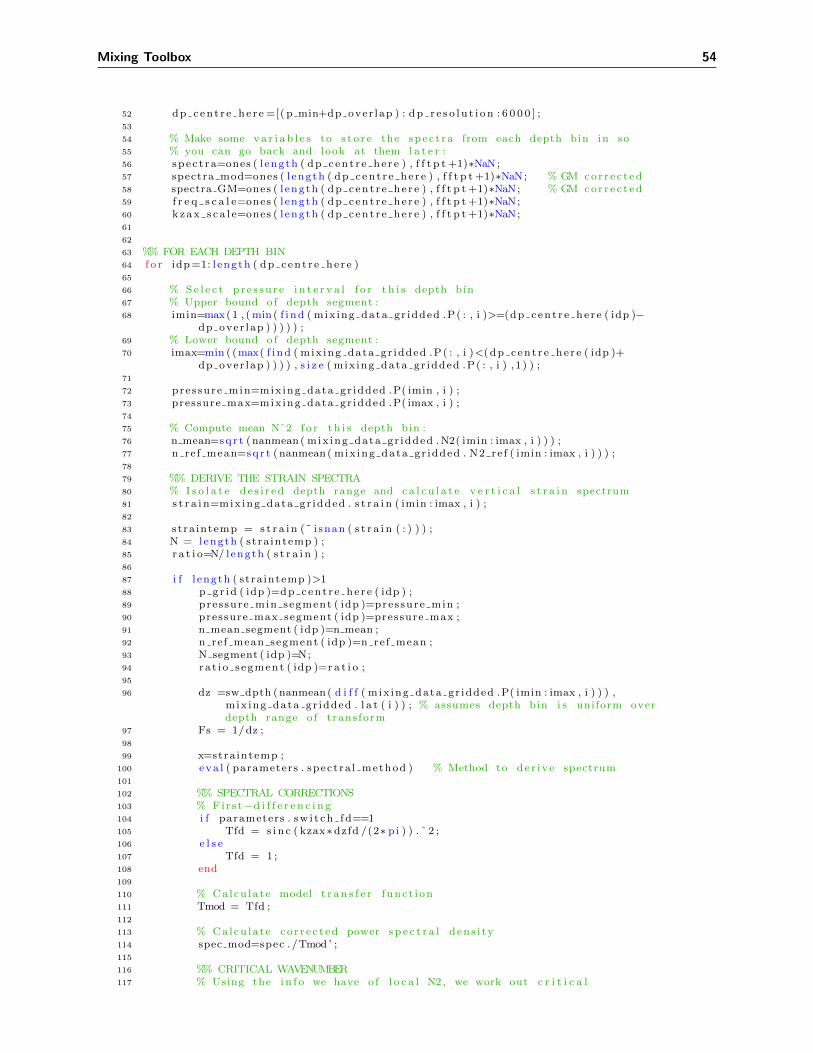
Mixing Toolbox 54

52 dp cen t r e he r e =[( p min+dp over lap ) : dp r e s o l u t i on : 6 0 0 0 ] ;53

54 % Make some va r i a b l e s to s t o r e the spec t ra from each depth bin in so55 % you can go back and look at them l a t e r :56 spec t ra=ones ( l ength ( dp cen t r e he r e ) , f f t p t +1)⇤NaN;57 spectra mod=ones ( l ength ( dp cen t r e he r e ) , f f t p t +1)⇤NaN; % GM cor r e c t ed58 spectra GM=ones ( l ength ( dp cen t r e he r e ) , f f t p t +1)⇤NaN; % GM cor r e c t ed59 f r e q s c a l e=ones ( l ength ( dp cen t r e he r e ) , f f t p t +1)⇤NaN;60 kzax s c a l e=ones ( l ength ( dp cen t r e he r e ) , f f t p t +1)⇤NaN;61

62

63 %% FOR EACH DEPTH BIN64 f o r idp=1: l ength ( dp cen t r e he r e )65

66 % Se l e c t p r e s su r e i n t e r v a l f o r t h i s depth bin67 % Upper bound o f depth segment :68 imin=max(1 , (min ( f i nd ( mix ing data gr idded .P( : , i )>=(dp cen t r e he r e ( idp )�

dp over lap ) ) ) ) ) ;69 % Lower bound o f depth segment :70 imax=min ( (max( f i nd ( mix ing data gr idded .P( : , i )<( dp c en t r e he r e ( idp )+

dp over lap ) ) ) ) , s i z e ( mix ing data gr idded .P( : , i ) , 1 ) ) ;71

72 pres sure min=mix ing data gr idded .P( imin , i ) ;73 pressure max=mix ing data gr idded .P( imax , i ) ;74

75 % Compute mean Nˆ2 f o r t h i s depth bin :76 n mean=sq r t (nanmean( mix ing data gr idded .N2( imin : imax , i ) ) ) ;77 n ref mean=sq r t (nanmean( mix ing data gr idded . N2 re f ( imin : imax , i ) ) ) ;78

79 %% DERIVE THE STRAIN SPECTRA80 % I s o l a t e d e s i r ed depth range and c a l c u l a t e v e r t i c a l s t r a i n spectrum81 s t r a i n=mix ing data gr idded . s t r a i n ( imin : imax , i ) ;82

83 stra intemp = s t r a i n (˜ i snan ( s t r a i n ( : ) ) ) ;84 N = length ( stra intemp ) ;85 r a t i o=N/ length ( s t r a i n ) ;86

87 i f l ength ( stra intemp )>188 p g r id ( idp )=dp cen t r e he r e ( idp ) ;89 pressure min segment ( idp )=pressure min ;90 pressure max segment ( idp )=pressure max ;91 n mean segment ( idp )=n mean ;92 n ref mean segment ( idp )=n ref mean ;93 N segment ( idp )=N;94 ra t i o s egment ( idp )=r a t i o ;95

96 dz =sw dpth (nanmean( d i f f ( mix ing data gr idded .P( imin : imax , i ) ) ) ,mix ing data gr idded . l a t ( i ) ) ; % assumes depth bin i s uniform overdepth range o f trans form

97 Fs = 1/dz ;98

99 x=stra intemp ;100 eva l ( parameters . spect ra l method ) % Method to de r i v e spectrum101

102 %% SPECTRAL CORRECTIONS103 % Fir s t�d i f f e r e n c i n g104 i f parameters . sw i t ch fd==1105 Tfd = s i n c ( kzax⇤dzfd /(2⇤ pi ) ) . ˆ 2 ;106 e l s e107 Tfd = 1 ;108 end109

110 % Calcu la t e model t r a n s f e r func t i on111 Tmod = Tfd ;112

113 % Calcu la t e co r r e c t ed power s p e c t r a l dens i ty114 spec mod=spec . /Tmod ’ ;115

116 %% CRITICAL WAVENUMBER117 % Using the i n f o we have o f l o c a l N2 , we work out c r i t i c a l

Mixing Toolbox 55

118 % wavenumber (mc) which g i v e s us b e t t e r e s t imate o f the119 % minimum v e r t i c a l wavelength o f i n t e g r a t i o n :120

121 shea rva r i ance=kzax (2 ) ⇤cumsum( spec ) ;122 [ nnn , index ]=min ( abs ( shearvar iance �0.7) ) ;123 ind ( idp )=index ;124 c r i t i c a lm ( idp )=kzax ( index ) ;125 minwavelength ( idp )=1/ c r i t i c a lm ( idp ) ⇤2⇤ pi ;126 i f minwavelength ( idp )<12;127 minwavelength ( idp )=12;128 end129

130 %% LINEAR INTERPOLATION131 % Linea r l y i n t e r p o l a t e onto f i n e r f requency ax i s (makes i n t e g r a t i n g132 % between c e r t a i n wavelengths more accurate )133

134 lambda max=1/ f r e q (2 ) ;135 lambda min=1/ f r e q ( end ) ;136 wavelengths=lambda min : 1 : lambda max ;137 f r eq2 =1./wavelengths ;138

139 spec2 = in t e rp1 ( f req , spec , f r e q2 ) ;140 spec mod2 = in t e rp1 ( f req , spec mod , f r eq2 ) ;141 kzax2 = in t e rp1 ( f req , kzax , f r eq2 ) ;142

143 % Store spec t ra f o r t h i s depth bin so you can look at i t l a t e r :144 f o r i i =1: l ength ( spec2 )145 spec t ra ( idp , i i )=spec2 ( i i ) ;146 spectra mod ( idp , i i )=spec mod2 ( i i ) ;147 f r e q s c a l e ( idp , i i )=f r eq2 ( i i ) ;148 kzax s c a l e ( idp , i i )=kzax2 ( i i ) ;149 end150

151 spec=spec2 ;152 spec mod=spec mod2 ;153 kzax=kzax2 ;154 f r e q=f r eq2 ;155

156 %% INTEGRATED SHEAR VARIANCE157 % Consider the i n t e g r a t ed s t r a i n var iance between the two158 % wavelengths o f i n t e r e s t � t h i s i s the meat in the f i n e s t r u c tu r e159 % est imate o f mixing160

161 % Def ine lzmax and lzmin , the range o f v e r t i c a l162 % wavelengths o f i n t e g r a t i o n :163 lzmin ( idp )=minwavelength ( idp ) ;164 lzmax ( idp )=(2⇤ pi /min ( kzax ) )�1;165 % Or could have used the s e t wavelengths o f i n t e g r a t i o n :166 % lzmin ( idp )=l zm in f i x ed ;167 % lzmax ( idp )=lzmax f ixed ;168

169 % Int eg r a t e power s p e c t r a l dens i ty between lzmin and lzmax :170 imax int=min ( f i nd ( kzax<(2⇤ pi / lzmax ( idp ) ) ) ) ;171 im in i n t=max( f i nd ( kzax>(2⇤ pi / lzmin ( idp ) ) ) ) ;172

173 i f isempty ( im in in t )==0 & isempty ( imax int )==0174

175 [ rows columns ]= s i z e ( kzax ) ;176 i f rows˜=1177 kzax=kzax ’ ;178 end179 vector1=cat (2 , kzax ( im in in t ) , kzax ( im in in t : imax int ) , kzax (

imax int ) , kzax ( im in in t ) ) ;180

181 [ rows columns ]= s i z e ( spec mod ) ;182 i f rows˜=1183 spec mod=spec mod ’ ;184 end185

186 vector2=cat (2 , 0 , spec mod ( im in in t : imax int ) , 0 , 0 ) ;

Mixing Toolbox 56

187

188 % Integ ra t ed var iance :189 va r i a n c e i n t=po lyarea ( vector1 , vector2 ) ;190 v a r i a n c e i n t e g r a l ( idp )=va r i a n c e i n t ;191

192 kmin in t eg ra l ( idp )=kzax ( im in in t ) ;193 kmax integra l ( idp )=kzax ( imax int ) ;194 n o p t s i n t e g r a l ( idp )=imax int�im in i n t +1;195

196 %% DERIVE DISSIPATION AND DIFFUSIVITY197 % For norma l i za t i on purposes compute power s p e c t r a l dens i ty o f198 % v e r t i c a l s t r a i n f o r the GM76 model199

200 N2mean = n mean . ˆ 2 ;201 N2refmean = n ref mean . ˆ 2 ;202

203 fmean=abs ( sw f ( mix ing data gr idded . l a t ( i ) ) ) ;204

205 be ta s t a r=pi ⇤parameters . j s t a r / parameters . b⇤ s q r t ( N2refmean ) /parameters .N0 ;

206

207 % Power s p e c t r a l dens i ty o f v e r t i c a l d i sp lacement :208 ph i z e t a = parameters .E⇤parameters . bˆ3⇤ parameters .N0ˆ2/(2⇤

parameters . j s t a r ⇤ pi ⇤N2refmean ) ./(1+ kzax/ be ta s t a r ) . ˆ 2 ;209 % Power s p e c t r a l dens i ty o f v e r t i c a l s t r a i n :210 ph i e t a = kzax . ˆ 2 . ⇤ ph i z e t a ;211

212 f o r i i =1: l ength ( ph i e t a )213 spectra GM ( idp , i i )=ph i e t a ( i i ) ;214 end215

216 %% Int eg r a t e GM76 power s p e c t r a l dens i ty217 i f isempty ( im in in t )==0 & isempty ( imax int )==0218 vector1=cat (2 , kzax ( im in in t ) , kzax ( im in in t : imax int ) , kzax (

imax int ) , kzax ( im in in t ) ) ;219 [ rows columns ]= s i z e ( ph i e t a ) ;220

221 i f rows˜=1222 ph i e t a=phi e ta ’ ;223 end224

225 vector2=cat (2 , 0 , ph i e t a ( im in i n t : imax int ) , 0 , 0 ) ;226 GM variance int=po lyarea ( vector1 , vector2 ) ;227 GM var iance integra l ( idp )=GM variance int ;228 e l s e229 GM var iance integra l ( idp )=NaN;230 end231

232 % Save the N2refmean as new va r i a b l e : N2b ( f o r background N2)233 N2b( idp )=N2refmean ;234

235 % Compute d i s s i p a t i o n ra t e ( e p s i l o n ) from the i n t e g r a t ed236 % s t r a i n var iance237 % s t r a i n var iance normal ized to GM76:238 norm st ra in va r i ance ( idp )=v a r i a n c e i n t e g r a l ( idp ) ˆ2/

GM var iance integra l ( idp ) ˆ2 ;239 ep s i l o n ( idp )=parameters . e p s i l on0 ⇤N2refmean/parameters .N0ˆ2⇤

norm s t ra in va r i ance ( idp ) ;240

241 % Modify es imate o f e p s i l o n by a few f a c t o r s ( s ee Kurt ’ s papers242 % fo r d e t a i l s ) ; F i r s t a c o r r e c t i o n f a c t o r that depends on243 % la t i t u d e . Second a c o r r e c t i o n f a c t o r that depends on the244 % shear to s t r a i n r a t i o .245

246 extra1 = ( fmean/parameters . f 0 ) ⇤ acosh ( sq r t ( N2refmean ) /fmean ) /acosh ( parameters .N0/parameters . f 0 ) ;

247 ep s i l o n ( idp ) = ep s i l o n ( idp ) ⇤ extra1 ;248

249 extra2 = 1/(6⇤ s q r t (2 ) ) ⇤( parameters .R⇤( parameters .R+1) ) /( sq r t ( abs (parameters .R�1) ) ) ;

Mixing Toolbox 57

250 ep s i l o n ( idp )=ep s i l o n ( idp ) ⇤ extra2 ;251

252 % Fina l l y from ep s i l o n c a l c u l a t e d iapycna l d i f f u s i v i t y253 % (kappa ) assuming the Osborn r e l a t i o n :254 kappa ( idp )=parameters . gamma⇤ ep s i l o n ( idp ) /N2refmean ;255

256 % Add va r i a b l e s to f l o a t s t r u c tu r e :257 mix ing data gr idded . e p s i l o n s t r a i n ( idp , i )=ep s i l o n ( idp ) ;258 mix ing data gr idded . Kz s t ra in ( idp , i )=kappa ( idp ) ;259 mix ing data gr idded . P m stra in ( idp , i )=p gr id ( idp ) ;260 mix ing data gr idded . s t r a i n v a r i a n c e ( idp , i )=v a r i a n c e i n t e g r a l ( idp )

;261 mix ing data gr idded .N2b( idp , i )=N2b( idp ) ’ ’ ;262 mix ing data gr idded . c r i t iWave s t r a i n ( idp , i )=minwavelength ( idp ) ;263

264 end265 end266 end267

268 % Index down to which mixing value that can be t ru s t ed :269 i i max=max( f i nd ( p gr id <(p max�dp over lap ) ) ) ;270 mix ing data gr idded . e p s i l o n s t r a i n ( i i max+1:end , i )=NaN;271 mix ing data gr idded . Kz s t ra in ( i i max+1:end , i )=NaN;272 mix ing data gr idded . P m stra in ( i i max+1:end , i )=NaN;273 mix ing data gr idded .N2b( i i max+1:end , i )=NaN;274

275 end276


B.8.5 mx derive mixing shearstrain.m

1 %==========================================================================2 % mx der i v e mix ing shea r s t r a in3 %4 % DESCRIPTION:5 % Combines e s t imate s o f f i n e s t r u c t u r e e p s i l o n from shear6 % and s t r a i n by computing the c o r r e c t i o n f a c t o r dependent on the observed7 % ( as opposed to assumed ) shear to s t r a i n r a t i o .8 % Here uses the ” s t r a i gh t�up” shear to s t r a i n r a t i o and assumes that the9 % shear var iance i n t e g r a l and s t r a i n var iance i n t e g r a l have been c a l c u l a t ed

10 % using the same wavelength range o f i n t e g r a t i o n .11 %12 % INPUT:13 %14 % OUTPUT:15 % N2 re f = Brunt�Vaisa la Frequency squared from Polz in code [ 1/ s ˆ2

]16 %17 % AUTHOR: Alberto NAVEIRA GARABATO18 %19 % Rev i s i t ed by : Stephanie WATERMAN 201020 % Amelie MEYER June 201421 %22 % VERSION NUMBER: 1 .0 (25 th June , 2014)23 %24 %==========================================================================25

26 p r o f i l e s=length ( mix ing data gr idded . f l t i d ) ;27

28 f o r i =1: p r o f i l e s ; % For each p r o f i l e29 common p scale =1 :3 :1648 ;30 N2=mix ing data gr idded .N2 ( : , i ) ;31

32 %% SHEAR VARIANCE:33 sh ea r va r i an c e=ones ( l ength ( common p scale ) , 1 ) ⇤NaN;34 e p s i l o n s h e a r=ones ( l ength ( common p scale ) , 1 ) ⇤NaN;35

36 % Check i f the r e i s any shear data f o r that p r o f i l e . . .

Mixing Toolbox 58

37 check=f i nd ( i snan ( mix ing data gr idded . Kz shear )==0) ;38 i f isempty ( check )==1;39 % There was no shear data then add empty (NaN) v a r i a b l e s40 l i=length ( mix ing data gr idded .P( : , i ) ) ;41 mix ing data gr idded . ep s i l on SS ( 1 : l i , i )=NaN;42 mix ing data gr idded . Kz SS ( 1 : l i , i )=NaN;43 mix ing data gr idded . P m SS ( 1 : l i , i )=NaN;44 mix ing data gr idded .Rw( 1 : l i , i )=NaN;45

46 % I f the re are shear data then we de r i v e v a r i a b l e s :47 e l s e48 f o r idp=1: l ength ( mix ing data gr idded . P m shear ( : , i ) ) ;49 c l e a r i i j j50 i i=f i nd ( common p scale==mix ing data gr idded . P m shear ( idp , i )�(

dp r e s o l u t i on /2) ) ;51 j j=f i nd ( common p scale==mix ing data gr idded . P m shear ( idp , i )+(

dp r e s o l u t i on /2) ) ;52 f o r idp2=i i : j j53 % Copy va r i a b l e s from mixing data54 sh ea r va r i an c e ( idp2 )=mix ing data gr idded . sh ea r va r i an c e ( idp , i

) ;55 e p s i l o n s h e a r ( idp2 )=mix ing data gr idded . e p s i l o n s h e a r ( idp , i ) ;56 end57 end58

59 %% STRAIN60 % Pre�a l l o c a t e some va r i a b l e s61 s t r a i n v a r i a n c e=ones ( l ength ( common p scale ) , 1 ) ⇤NaN;62 e p s i l o n s t r a i n=ones ( l ength ( common p scale ) , 1 ) ⇤NaN;63 N2b=ones ( l ength ( common p scale ) , 1 ) ⇤NaN;64 mix ing data gr idded . P m shear ( i snan ( mix ing data gr idded . P m shear ) )

=0;65 % Works out hom many d index apart shear and s t r a i n are :66 d=mix ing data gr idded . P m shear (1 , i )�mix ing data gr idded . P m stra in

(1 , i ) /3 ;67 i f d>368 d=0;69 end70 i f d<071 d=0;72 end73

74 f o r idp=1: l ength ( mix ing data gr idded . P m stra in ( : , i ) ) ;75 c l e a r i i 2 j j 276 i i 2=f i nd ( common p scale==mix ing data gr idded . P m stra in ( idp , i )�(

dp r e s o l u t i on /2) ) ;77 j j 2=f i nd ( common p scale==mix ing data gr idded . P m stra in ( idp , i )+(

dp r e s o l u t i on /2) ) ;78 % Moving a l l e p s i s t r a i n by 1 index down to match ep s i79 % shear s c a l e :80 f o r idp2=i i 2 : j j 281 % Copy va r i a b l e s from mixing data82 s t r a i n v a r i a n c e ( idp2+d)=mix ing data gr idded . s t r a i n v a r i a n c e (

idp , i ) ;83 e p s i l o n s t r a i n ( idp2+d)=mix ing data gr idded . e p s i l o n s t r a i n ( idp

, i ) ;84 N2b( idp2+d)=mix ing data gr idded .N2b( idp , i ) ;85 end86 end87

88 %% FIND POINT OF MAX N2 IN WATER COLUMN89 [ crap ind ]=max(N2) ;90 depth ( i )=common p scale ( ind ) ;91 t r e shho ld ( i )=depth ( i )+dp over lap ;92 [ crap index t r e shho ld ( i ) ]=min ( abs ( t r e shho ld ( i )�common p scale ) ) ;93

94 %% DERIVE SHEAR STRAIN RATIO95 Rw=shea r va r i an c e . / s t r a i n v a r i a n c e ;96 % Replace Rw va lue s in su r f a c e waters with a mean Rw97 Rw(1 : i ndex t r e shho ld ( i ) )=5; % 5 i s the mean Rw f o r the data s e t

Mixing Toolbox 59

98

99 % Apply ext ra f a c t o r mu l t ip ly ing ep s i l o n depending100 % on shear to s t r a i n r a t i o us ing ac tua l shear to s t r a i n r a t i o :101 h=r e a l ( ( 3⇤ (Rw+1) ) . / ( 2⇤ s q r t (2 ) .⇤Rw. ⇤ ( (Rw�1) ) . ˆ ( 1 /2 ) ) ) ;102

103 % Remove constant Rw app l i ed :104 ep s i l o n=ep s i l o n s h e a r ;105 extra2 =(3⇤( parameters .R+1) ) . / ( 2⇤ s q r t (2 ) .⇤ parameters .R. ⇤ ( ( parameters .R

�1) ) . ˆ ( 1 /2 ) ) ;106 ep s i l on2=ep s i l o n / extra2 ;107

108 % Apply va r i ab l e Rw:109 e p s i l o n s h e a r a nd s t r a i n=ep s i l on2 .⇤h ;110

111 % Fina l l y from ep s i l o n c a l c u l a t e d iapycna l d i f f u s i v i t y112 % (kappa ) assuming the Osborn r e l a t i o n :113 kappa=parameters . gamma⇤ e p s i l o n s h e a r a nd s t r a i n . /N2b ;114

115 % Add va r i a b l e s to f l o a t s t r u c tu r e :116 mix ing data gr idded . e p s i l o n ( : , i )=ep s i l o n s h e a r a nd s t r a i n ;117 mix ing data gr idded .Kz ( : , i )=kappa ;118 mix ing data gr idded .P m( : , i )=common p scale ;119 mix ing data gr idded .Rw( : , i )=Rw;120 end121 end122

123 % Remove a va r i ab l e from the f l o a t s t r u c tu r e124 mix ing data gr idded=rmf i e l d ( mix ing data gr idded , ’N2b ’ ) ;125

126 eva l ( [ ’ save ( ’ ’ m ix ing data gr idded ’ run ’ . mat ’ ’ , ’ ’�regexp ’ ’ , ’ ’ ˆmix ing data gr idded ’ ’ , ’ ’ ˆ f l t ’ ’ ) ’ ] ) ;

B.9 Plot mixing variables

B.9.1 mx plot dissipation rate.m

1 f unc t i on [ ] = mx p l o t d i s s i p a t i o n r a t e ( f i g , d i r e c to ry , run )2

3 % mx p l o t d i s s i p a t i o n r a t e Plot the d i s s i p a t i o n ra t e4 %==========================================================================5 %6 % USAGE:7 % [ ] = mx p l o t d i s s i p a t i o n r a t e ( f i g , d i r e c to ry , run )8 %9 % DESCRIPTION:

10 % Plot a l l the d i s s i p a t i o n ra t e p r o f i l e s .11 %12 % INPUT:13 % f i g = e i t h e r ’ on ’ or ’ o f f ’ to utrn f i g d i sp l ay on and o f f14 % d i r e c t o r y = path o f d i r e c t o r y where f i g u r e i s saved15 %16 % OUTPUT:17 % Figure : / d i s s i p a t i o n r a t e . eps18 %19 % AUTHOR:20 % Amelie MEYER21 %22 % VERSION NUMBER: 1 .0 (26 rd June , 2014)23 %24 % RERENCE: A. Meyer , B.M. Sloyan , K.L . Polz in , H.E. Ph i l l i p s , and N.L .25 % Bindof f . Mixing v a r i a b i l i t y in the Southern Ocean . Journal o f26 % Phys i ca l Oceanography , 45 ,966�987 , 2015 .27 %==========================================================================28 di sp ( ’ Plot the d i s s i p a t i o n ra t e ( e p s i l o n ) . . . ’ )29

30 eva l ( [ ’ load mix ing data gr idded ’ run ’ . mat ’ ] ) ;31

Mixing Toolbox 60

32 %% Plot o f d i s s i p a t i o n along p r o f i l e numbers33 nb p r o f i l e s=length ( mix ing data gr idded . f l t i d ) ;34 mini=min (min ( mix ing data gr idded . e p s i l o n ) ) ;35 maxi=max(max( mix ing data gr idded . e p s i l o n ) ) ;36 ep s i l o n=mix ing data gr idded . e p s i l o n ;37 ep s i l o n ( f i nd ( ep s i l o n==0))=NaN;38


f i g u r e width=1000 f o r f i r s t p l o t42 eva l ( [ ’ s e t (3 , ’ ’ v i s i b l e ’ ’ , ’ ’ ’ f i g ’ ’ ’ ) ; ’ ] )43 imagesc ( 1 : n b p r o f i l e s , mix ing data gr idded .P( : , 1 ) , log10 ( ep s i l o n ) ) ;44 hold on45 ax i s i j46 s e t ( gca , ’ Po s i t i on ’ , [ 0 . 0 8 8 0 .13 0 .87 0 . 7 7 ] ) % po s i t i o n o f p l o t in f i g u r e47 colormap ( rot90 ( hot , 2 ) ) ;48 h=co l o rba r ;49 s e t ( get (h , ’ y l ab e l ’ ) , ’ s t r i n g ’ , ’ l o g {10}(\ ep s i l o n ) [mˆ{2} s ˆ{�3}] ’ , ’ f o n t s i z e ’

, 10) ;50 c ax i s ( [ log10 ( mini ) log10 (maxi ) ] )51 xlim ( [ 0 l ength ( mix ing data gr idded . p ro f i l e number ) ] )52 ylim ( [ 0 1600 ] ) ;53 x l ab e l ( ’ Cumulative p r o f i l e number ’ , ’ FontSize ’ , 10) ;54 y l ab e l ( ’ Pressure [ dbar ] ’ , ’ FontSize ’ , 10)55

56 %% Density contour57 s igma 0=mix ing data gr idded . s igma 0 ;58 [C, h]= contour ( 1 : l ength ( mix ing data gr idded . p ro f i l e number ) ,

mix ing data gr idded .P( : , 1 ) , sigma 0 , [ 2 7 : 0 . 1 : 2 9 ] , ’ c o l o r ’ , [ 0 . 6 0 . 6 0 . 6 ] , ’l i n ew id th ’ , 1 ) ;

59


62 %% Saving f i g u r e opt ions63 s e t ( gcf , ’ PaperPositionMode ’ , ’ auto ’ )64 s e t ( gcf , ’ r ende r e r ’ , ’ p a i n t e r s ’ )65 s i gna tu r e ( ’ I n i t i a l a n a l y s i s ’ , ’ ’ )66 pr in t (h2 , ’�depsc2 ’ , [ ’ ’ d i r e c t o r y ’ / f i g u r e s / d i s s i p a t i o n r a t e . eps ’ ] ) ;

B.9.2 mx plot di↵usivity.m

1 f unc t i on [ ] = mx p l o t d i f f u s i v i t y ( f i g , d i r e c to ry , run )2

3 % mx p l o t d i f f u s i v i t y Plot the d i f f u s i v i t y4 %==========================================================================5 %6 % USAGE:7 % [ ] = mx p l o t d i f f u s i v i t y ( f i g , d i r e c to ry , run )8 %9 % DESCRIPTION:

10 % Plot a l l the d i f f u s i v i t y p r o f i l e s11 %12 % INPUT:13 % f i g = e i t h e r ’ on ’ or ’ o f f ’ to utrn f i g d i sp l ay on and o f f14 % d i r e c t o r y = path o f d i r e c t o r y where f i g u r e i s saved15 %16 % OUTPUT:17 % Figure : / d i f f u s i v i t y . eps18 %19 % AUTHOR:20 % Amelie MEYER21 %22 % VERSION NUMBER: 1 .0 (26 rd June , 2014)23 %24 % RERENCE: A. Meyer , B.M. Sloyan , K.L . Polz in , H.E. Ph i l l i p s , and N.L .25 % Bindof f . Mixing v a r i a b i l i t y in the Southern Ocean . Journal o f26 % Phys i ca l Oceanography , 45 ,966�987 , 2015 .27 %==========================================================================

Mixing Toolbox 61

28 di sp ( ’ Plot the d i f f u s i v i t y ( kappa ) . . . ’ )29

30 eva l ( [ ’ load mix ing data gr idded ’ run ’ . mat ’ ] ) ;31 load pr i va t e1 / o th e r c o l o r / co lorData .mat Msunsetco lors32

33 %% Plot o f d i s s i p a t i o n along p r o f i l e numbers34 nb p r o f i l e s=length ( mix ing data gr idded . f l t i d ) ;35 mini=min (min ( mix ing data gr idded .Kz) ) ;36 maxi=max(max( mix ing data gr idded .Kz) ) ;37 d i f f u s i v i t y=mix ing data gr idded .Kz ;38 d i f f u s i v i t y ( f i nd ( d i f f u s i v i t y==0))=NaN;39


f i g u r e width=1000 f o r f i r s t p l o t43 eva l ( [ ’ s e t (3 , ’ ’ v i s i b l e ’ ’ , ’ ’ ’ f i g ’ ’ ’ ) ; ’ ] )44 imagesc ( 1 : n b p r o f i l e s , mix ing data gr idded .P( : , 1 ) , log10 ( d i f f u s i v i t y ) ) ;45 hold on46 ax i s i j47 s e t ( gca , ’ Po s i t i on ’ , [ 0 . 0 8 8 0 .13 0 .87 0 . 7 7 ] ) % po s i t i o n o f p l o t in f i g u r e48 colormap ( f l i p ud ( Msunsetco lors ) ) ;49 h=co l o rba r ;50 s e t ( get (h , ’ y l ab e l ’ ) , ’ s t r i n g ’ , ’ l o g {10}(K {z }) [mˆ{2} s ˆ{�1}] ’ , ’ f o n t s i z e ’ , 10) ;51 c ax i s ( [ log10 ( mini ) log10 (maxi ) ] )52 xlim ( [ 0 l ength ( mix ing data gr idded . p ro f i l e number ) ] )53 ylim ( [ 0 1600 ] ) ;54 x l ab e l ( ’ Cumulative p r o f i l e number ’ , ’ FontSize ’ , 10) ;55 y l ab e l ( ’ Pressure [ dbar ] ’ , ’ FontSize ’ , 10)56



60


63 %% Saving f i g u r e opt ions64 s e t ( gcf , ’ PaperPositionMode ’ , ’ auto ’ )65 s e t ( gcf , ’ r ende r e r ’ , ’ p a i n t e r s ’ )66 s i gna tu r e ( ’ I n i t i a l a n a l y s i s ’ , ’ ’ )67 pr in t (h2 , ’�depsc2 ’ , [ ’ ’ d i r e c t o r y ’ / f i g u r e s / d i f f u s i v i t y . eps ’ ] ) ;

B.9.3 mx plot CCW CW.m

1 f unc t i on [ ] = mx plot CCW CW( f i g , d i r e c to ry , run )2

3 % mx plot CCW CW Plot the CCW / CW ra t i o4 %==========================================================================5 %6 % USAGE:7 % [ ] = mx plot CCW CW( f i g , d i r e c to ry , run )8 %9 % DESCRIPTION:

10 % Plot a l l the r a t i o o f ro ta ry shear var iance p r o f i l e s .11 %12 % INPUT:13 % f i g = e i t h e r ’ on ’ or ’ o f f ’ to utrn f i g d i sp l ay on and o f f14 % d i r e c t o r y = path o f d i r e c t o r y where f i g u r e i s saved15 %16 % OUTPUT:17 % Figure : /CCWCW. eps18 %19 % AUTHOR:20 % Amelie MEYER21 %22 % VERSION NUMBER: 1 .0 (26 rd June , 2014)23 %

Mixing Toolbox 62

24 % RERENCE: A. Meyer , B.M. Sloyan , K.L . Polz in , H.E. Ph i l l i p s , and N.L .25 % Bindof f . Mixing v a r i a b i l i t y in the Southern Ocean . Journal o f26 % Phys i ca l Oceanography , 45 ,966�987 , 2015 .27 %==========================================================================28 di sp ( ’ Plot the CCW / CW ra t i o . . . ’ )29


32 %% Plot33 nb p r o f i l e s=length ( mix ing data gr idded . f l t i d ) ;34 CCW=mix ing data gr idded . CCW S variance ;35 CW=mix ing data gr idded . CW S variance ;36


f i g u r e width=1000 f o r f i r s t p l o t40 eva l ( [ ’ s e t (3 , ’ ’ v i s i b l e ’ ’ , ’ ’ ’ f i g ’ ’ ’ ) ; ’ ] )41 imagesc ( 1 : n b p r o f i l e s , mix ing data gr idded .P( : , 1 ) , log10 (CCW./CW) ) ;42 hold on43 ax i s i j44 s e t ( gca , ’ Po s i t i on ’ , [ 0 . 0 8 8 0 .13 0 .87 0 . 7 7 ] ) % po s i t i o n o f p l o t in f i g u r e45 colormap ( f l i p ud ( hot ) ) ;46 h=co l o rba r ;47 s e t ( get (h , ’ y l ab e l ’ ) , ’ s t r i n g ’ , ’ l o g {10} CCW/CW shear var iance r a t i o ’ , ’ f o n t s i z e

’ , 10) ;48 c ax i s ([�1 1 ] )49 xlim ( [ 0 l ength ( mix ing data gr idded . p ro f i l e number ) ] )50 ylim ( [ 0 1600 ] ) ;51 x l ab e l ( ’ Cumulative p r o f i l e number ’ , ’ FontSize ’ , 10) ;52 y l ab e l ( ’ Pressure [ dbar ] ’ , ’ FontSize ’ , 10)53



57


60 %% Saving f i g u r e opt ions61 s e t ( gcf , ’ PaperPositionMode ’ , ’ auto ’ )62 s e t ( gcf , ’ r ende r e r ’ , ’ p a i n t e r s ’ )63 s i gna tu r e ( ’ I n i t i a l a n a l y s i s ’ , ’ ’ )64 pr in t (h2 , ’�depsc2 ’ , [ ’ ’ d i r e c t o r y ’ / f i g u r e s /CCWCW. eps ’ ] ) ;

B.9.4 mx plot Rw.m

1 f unc t i on [ ] = mx plot Rw ( f i g , d i r e c to ry , run )2

3 % mx plot Rw Plot the shear / s t r a i n r a t i o (Rw)4 %==========================================================================5 %6 % USAGE:7 % [ ] = mx plot Rw ( f i g , d i r e c to ry , run )8 %9 % DESCRIPTION:

10 % Plot a l l the shear�to�s t r a i n var iance r a t i o p r o f i l e s .11 %12 % INPUT:13 % f i g = e i t h e r ’ on ’ or ’ o f f ’ to utrn f i g d i sp l ay on and o f f14 % d i r e c t o r y = path o f d i r e c t o r y where f i g u r e i s saved15 %16 % OUTPUT:17 % Figure : /Rw. eps18 %19 % AUTHOR:20 % Amelie MEYER21 %

Mixing Toolbox 63

22 % VERSION NUMBER: 1 .0 (26 rd June , 2014)23 %24 % RERENCE: A. Meyer , B.M. Sloyan , K.L . Polz in , H.E. Ph i l l i p s , and N.L .25 % Bindof f . Mixing v a r i a b i l i t y in the Southern Ocean . Journal o f26 % Phys i ca l Oceanography , 45 ,966�987 , 2015 .27 %==========================================================================28 di sp ( ’ Plot the shear / s t r a i n r a t i o (Rw) . . . ’ )29


32 %% Plot33 nb p r o f i l e s=length ( mix ing data gr idded . f l t i d ) ;34 Rw=mix ing data gr idded .Rw;35 mini=min (min ( mix ing data gr idded .Rw) ) ;36 maxi=max(max( mix ing data gr idded .Rw) ) ;37


f i g u r e width=1000 f o r f i r s t p l o t41 eva l ( [ ’ s e t (3 , ’ ’ v i s i b l e ’ ’ , ’ ’ ’ f i g ’ ’ ’ ) ; ’ ] )42 imagesc ( 1 : n b p r o f i l e s , mix ing data gr idded .P( : , 1 ) ,Rw) ;43 hold on44 ax i s i j45 s e t ( gca , ’ Po s i t i on ’ , [ 0 . 0 8 8 0 .13 0 .87 0 . 7 7 ] ) % po s i t i o n o f p l o t in f i g u r e46 colormap ( f l i p ud ( f l i p l r ( hot ) ) ) ;47 h=co l o rba r ;48 s e t ( get (h , ’ y l ab e l ’ ) , ’ s t r i n g ’ , ’R \omega ’ , ’ f o n t s i z e ’ , 10) ;49 c ax i s ( [ mini maxi ] )50 xlim ( [ 0 l ength ( mix ing data gr idded . p ro f i l e number ) ] )51 ylim ( [ 0 1600 ] ) ;52 x l ab e l ( ’ Cumulative p r o f i l e number ’ , ’ FontSize ’ , 10) ;53 y l ab e l ( ’ Pressure [ dbar ] ’ , ’ FontSize ’ , 10)54



58


61 %% Saving f i g u r e opt ions62 s e t ( gcf , ’ PaperPositionMode ’ , ’ auto ’ )63 s e t ( gcf , ’ r ende r e r ’ , ’ p a i n t e r s ’ )64 s i gna tu r e ( ’ I n i t i a l a n a l y s i s ’ , ’ ’ )65 pr in t (h2 , ’�depsc2 ’ , [ ’ ’ d i r e c t o r y ’ / f i g u r e s /Rw. eps ’ ] ) ;

B.10 Function to check the installation of the library

B.10.1 mx check functions.m

1

2 i f isempty ( which ( ’ l a s tgood2 .m’ ) )3 f p r i n t f (2 , ’You need to add the MX ” pr iva t e1 ” subd i r e c to ry to your path . \

n ’ ) ;4 end5

6 i f isempty ( which ( ’ l a s tgood2 .m’ ) )7 e r r o r ( ’You have not added the MX subd i r e c t o r i e s to you MATLAB Path ’ )8 end9

10 f l o a t d a t a=’ f l oat data vmx ’ ;11 run=’ t e s t ’ ;12 f i g=’ o f f ’ ;13 dummy = which ( ’ l a s tgood2 .m’ ) ;14 d i r e c t o r y = [dummy( 1 : end�20) ] ;

Mixing Toolbox 64

15 mx parameters=’ mx parameters ’ ;16

17 f p r i n t f (1 , ’ \n ’ ) ;18 f p r i n t f (1 , ’ This func t i on i s running 36 s to r ed v e r t i c a l p r o f i l e s o f

temperature , \n ’ ) ;19 f p r i n t f (1 , ’ s a l i n i t y and ho r i z on t a l v e l o c i t y from the EM�APEX f l o a t 3951

through\n ’ ) ;20 f p r i n t f (1 , ’ a l l the f unc t i on s in the MX Oceanographic Toolbox .\n ’ ) ;21 f p r i n t f (1 , ’ \n ’ ) ;22

23 mx cf . mx chks = 1 ;24

25

26 %% Check value o f cons tant s and parameters in mx parameters . mat27 load ( mx parameters ) ;28

29 f p r i n t f (1 , ’ \n ’ ) ;30 f p r i n t f (1 , ’ Check value o f cons tant s and parameters \n ’ ) ;31 f p r i n t f (1 , ’ in the parameter f i l e mx parameters . mat \n ’ ) ;32 f p r i n t f (1 , ’ \n ’ ) ;33

34 U = parameters .U;35 i f eva l ( [ ’ ’ U ’�1 ’ ] ) > 1e�1336 f p r i n t f (2 , ’ Parameter U: Fa i l ed \n ’ ) ;37 mx cf . mx chks = 0 ;38 end39

40 V = parameters .V;41 i f eva l ( [ ’ ’ V ’�1 ’ ] ) > 1e�1342 f p r i n t f (2 , ’ Parameter V: Fa i l ed \n ’ ) ;43 mx cf . mx chks = 0 ;44 end45

46 i f abs ( parameters . moving window � 20) > 1e�1347 f p r i n t f (2 , ’ Parameter moving window : Fa i l ed \n ’ ) ;48 mx cf . mx chks = 0 ;49 end50

51 i f abs ( parameters . dzN2ref � 24) > 1e�1352 f p r i n t f (2 , ’ Parameter dzN2ref : Fa i l ed \n ’ ) ;53 mx cf . mx chks = 0 ;54 end55

56 i f abs ( parameters . dzN2 � 6) > 1e�1357 f p r i n t f (2 , ’ Parameter dzN2 : Fa i l ed \n ’ ) ;58 mx cf . mx chks = 0 ;59 end60

61 i f abs ( parameters . drho � 0 . 03 ) > 1e�1362 f p r i n t f (2 , ’ Parameter drho : Fa i l ed \n ’ ) ;63 mx cf . mx chks = 0 ;64 end65

66 i f abs ( parameters . dz � 3) > 1e�1367 f p r i n t f (2 , ’ Parameter dz : Fa i l ed \n ’ ) ;68 mx cf . mx chks = 0 ;69 end70

71 i f abs ( parameters . dzs � 6) > 1e�1372 f p r i n t f (2 , ’ Parameter dzs : Fa i l ed \n ’ ) ;73 mx cf . mx chks = 0 ;74 end75

76 i f abs ( parameters . f f t p t � 128) > 1e�1377 f p r i n t f (2 , ’ Parameter f f t p t : Fa i l ed \n ’ ) ;78 mx cf . mx chks = 0 ;79 end80

81 i f abs ( parameters . l zm in f i x ed � 50) > 1e�1382 f p r i n t f (2 , ’ Parameter l zm in f i x ed : Fa i l ed \n ’ ) ;

Mixing Toolbox 65

83 mx cf . mx chks = 0 ;84 end85

86 i f abs ( parameters . l zmax f ixed � 300) > 1e�1387 f p r i n t f (2 , ’ Parameter l zmax f ixed : Fa i l ed \n ’ ) ;88 mx cf . mx chks = 0 ;89 end90

91 i f abs ( parameters .R � 5) > 1e�1392 f p r i n t f (2 , ’ Parameter R: Fa i l ed \n ’ ) ;93 mx cf . mx chks = 0 ;94 end95

96 i f abs ( parameters . gamma � 0 . 2 ) > 1e�1397 f p r i n t f (2 , ’ Parameter gamma: Fa i l ed \n ’ ) ;98 mx cf . mx chks = 0 ;99 end

100

101 i f abs ( parameters . e p s i l on0 � 8e�10) > 1e�13102 f p r i n t f (2 , ’ Parameter ep s i l on0 : Fa i l ed \n ’ ) ;103 mx cf . mx chks = 0 ;104 end105

106 i f abs ( parameters .N0 � 0 .0052) > 1e�4107 f p r i n t f (2 , ’ Parameter N0 : Fa i l ed \n ’ ) ;108 mx cf . mx chks = 0 ;109 end110

111 i f abs ( parameters . f 0 � 7 .8360 e�5) > 1e�8112 f p r i n t f (2 , ’ Parameter f 0 : Fa i l ed \n ’ ) ;113 mx cf . mx chks = 0 ;114 end115

116 i f abs ( parameters .E � 6 .3 e�5) ˜= 0117 f p r i n t f (2 , ’ Parameter E: Fa i l ed \n ’ ) ;118 mx cf . mx chks = 0 ;119 end120

121 i f abs ( parameters . b � 1300) > 1e�13122 f p r i n t f (2 , ’ Parameter b : Fa i l ed \n ’ ) ;123 mx cf . mx chks = 0 ;124 end125

126 i f abs ( parameters . j s t a r � 3) > 1e�13127 f p r i n t f (2 , ’ Parameter j s t a r : Fa i l ed \n ’ ) ;128 mx cf . mx chks = 0 ;129 end130

131 spectra lmethod = parameters . spect ra l method ;132 s t r i n g=’Tycho2 ’ ;133 i f eva l ( ’ spectra lmethod ’ ) ˜= eva l ( ’ s t r i n g ’ )134 f p r i n t f (2 , ’ Parameter spect ra l method : Fa i l ed \n ’ ) ;135 mx cf . mx chks = 0 ;136 end137

138 cospectra lmethod = parameters . cospect ra l method ;139 s t r i n g=’ Tycho2 cospectra ’ ;140 i f eva l ( ’ cospectra lmethod ’ ) ˜= eva l ( ’ s t r i n g ’ )141 f p r i n t f (2 , ’ Parameter cospect ra l method : Fa i l ed \n ’ ) ;142 mx cf . mx chks = 0 ;143 end144

145 i f abs ( parameters . sw i t ch fd � 1) > 1e�13146 f p r i n t f (2 , ’ Parameter sw i t ch fd : Fa i l ed \n ’ ) ;147 mx cf . mx chks = 0 ;148 end149

150 i f i snan ( parameters . c r i t r a t ) ˜= 1151 f p r i n t f (2 , ’ Parameter c r i t r a t : Fa i l ed \n ’ ) ;152 mx cf . mx chks = 0 ;

Mixing Toolbox 66

153 end154

155 i f i snan ( parameters . l zm in th r e sho ld ) ˜= 1156 f p r i n t f (2 , ’ Parameter l zm in th r e sho ld : Fa i l ed \n ’ ) ;157 mx cf . mx chks = 0 ;158 end159

160 c l e a r E N0 R U V b cospectra lmethod c r i t r a t drho dz dzN2ref dzN2 dzs ep s i l on0f0 f f t p t gamma j s t a r lzmaxf ixed l zm in f i x ed l zminthre sho ld movingwindow

spectra lmethod s t r i n g swi t ch fd161

162 %% Load and bu i ld da ta s e t s163 i f e x i s t ( ’ parameters ’ , ’ var ’ )==0;164 f p r i n t f (2 , ’ load parameters : Fa i l ed \n ’ ) ;165 mx cf . mx chks = 0 ;166 end167

168 mx bu i l d i n i t i a l d a t a ( f l o a t d a t a )169 i f e x i s t ( ’ i n i t i a l d a t a . mat ’ , ’ f i l e ’ )==0;170 f p r i n t f (2 , ’ mx bu i l d i n i t i a l d a t a : Fa i l ed \n ’ ) ;171 mx cf . mx chks = 0 ;172 end173

174 %% Derive f a l l r a t e o f the EM�APEX f l o a t s175 mx de r i v e f a l l r a t e176 load i n i t i a l d a t a . mat177 i f isempty ( [ ’ F l t ’ i n t 2 s t r ( f l t ) ’ ( 1 ) . f a l l r a t e ) ’ ] ) ;178 f p r i n t f (2 , ’ mx d e r i v e f a l l r a t e : Fa i l ed \n ’ ) ;179 mx cf . mx chks = 0 ;180 end181 c l e a r ( [ ’ F l t ’ i n t 2 s t r ( f l t ) ’ ’ ] )182 c l e a r f l t183

184 %% Grid CTD data onto 2 .2 dbar and EM on 3dbar185 mx g r i d i n i t i a l d a t a ( parameters .U, parameters .V)186

187 %% Derive i n i t i a l v a r i a b l e s188 mx der ive abs T S189 mx der iv e po t en t i a l d en s i ty anoma ly190 mx derive N2 ( parameters . dzN2)191 mx der ive mixed layer depth ( parameters . drho )192 mx der ive cur r ent speed193


196 i f isempty ( [ ’ f l o a t ’ i n t 2 s t r ( f l t ) ’ ( 1 ) .SA) ’ ] ) ==1;197 f p r i n t f (2 , ’ mx der ive abs T S : Fa i l ed \n ’ ) ;198 mx cf . mx chks = 0 ;199 end200 i f isempty ( [ ’ f l o a t ’ i n t 2 s t r ( f l t ) ’ ( 1 ) .CT) ’ ] ) ==1;201 f p r i n t f (2 , ’ mx der ive abs T S : Fa i l ed \n ’ ) ;202 mx cf . mx chks = 0 ;203 end204 i f isempty ( [ ’ f l o a t ’ i n t 2 s t r ( f l t ) ’ ( 1 ) . s igma 0 ) ’ ] ) ==1;205 f p r i n t f (2 , ’ mx de r i v e po t en t i a l d en s i ty anoma ly : Fa i l ed \n ’ ) ;206 mx cf . mx chks = 0 ;207 end208 i f isempty ( [ ’ f l o a t ’ i n t 2 s t r ( f l t ) ’ ( 1 ) .N2) ’ ] ) ==1;209 f p r i n t f (2 , ’ mx derive N2 : Fa i l ed \n ’ ) ;210 mx cf . mx chks = 0 ;211 end212 i f isempty ( [ ’ f l o a t ’ i n t 2 s t r ( f l t ) ’ ( 1 ) .MLD) ’ ] ) ==1;213 f p r i n t f (2 , ’ mx der ive mixed layer depth : Fa i l ed \n ’ ) ;214 mx cf . mx chks = 0 ;215 end216 i f isempty ( [ ’ f l o a t ’ i n t 2 s t r ( f l t ) ’ ( 1 ) . speed ) ’ ] ) ==1;217 f p r i n t f (2 , ’ mx der ive cur r ent speed : Fa i l ed \n ’ ) ;218 mx cf . mx chks = 0 ;219 end220

Mixing Toolbox 67

221 c l e a r ( [ ’ f l o a t ’ i n t 2 s t r ( f l t ) ’ ’ ] )222 c l e a r f l t223

224 %% Plot main v a r i a b l e s225 f p r i n t f (1 , ’ \n ’ ) ;226 f p r i n t f (1 , ’The d e f au l t s e t up f o r the MX ana l y s i s i s that output \n ’ ) ;227 f p r i n t f (1 , ’ f i g u r e s are turned o f f ( do not appear on the s c r e en ) \n ’ ) ;228 f p r i n t f (1 , ’ and are saved in s t ead in the ’ ’ f i g u r e s ’ ’ f o l d e r .\n ’ ) ;229 f p r i n t f (1 , ’ \n ’ ) ;230

231 mx g r i d a l l i n i t i a l d a t a232 i f e x i s t ( ’ i n i t i a l d a t a g r i d d e d .mat ’ , ’ f i l e ’ )==0;233 f p r i n t f (2 , ’ m x g r i d a l l i n i t i a l d a t a : Fa i l ed \n ’ ) ;234 mx cf . mx chks = 0 ;235 end236

237 mx plot temperature ( f i g , d i r e c t o r y )238 mx p l o t s a l i n i t y ( f i g , d i r e c t o r y )239 mx plot N2 ( f i g , d i r e c t o r y )240 mx plot mixed layer depth ( f i g , d i r e c t o r y )241 mx plo t cur r ent speed ( f i g , d i r e c t o r y )242 i f e x i s t ( [ d i r e c to ry , ’ f i g u r e s ’ , d i r e c t o r y ( end ) , ’ temperature . eps ’ ] , ’ f i l e ’ )==0;243 f p r i n t f (2 , ’ mx plot temperature : Fa i l ed \n ’ ) ;244 mx cf . mx chks = 0 ;245 end246 i f e x i s t ( [ d i r e c to ry , ’ f i g u r e s ’ , d i r e c t o r y ( end ) , ’ s a l i n i t y . eps ’ ] , ’ f i l e ’ )==0;247 f p r i n t f (2 , ’ mx p l o t s a l i n i t y : Fa i l ed \n ’ ) ;248 mx cf . mx chks = 0 ;249 end250 i f e x i s t ( [ d i r e c to ry , ’ f i g u r e s ’ , d i r e c t o r y ( end ) , ’N2 . eps ’ ] , ’ f i l e ’ )==0;251 f p r i n t f (2 , ’ mx plot N2 : Fa i l ed \n ’ ) ;252 mx cf . mx chks = 0 ;253 end254 i f e x i s t ( [ d i r e c to ry , ’ f i g u r e s ’ , d i r e c t o r y ( end ) , ’ mixed layer depth . eps ’ ] , ’ f i l e ’ )

==0;255 f p r i n t f (2 , ’ mx plot mixed layer depth : Fa i l ed \n ’ ) ;256 mx cf . mx chks = 0 ;257 end258 i f e x i s t ( [ d i r e c to ry , ’ f i g u r e s ’ , d i r e c t o r y ( end ) , ’ cu r r en t speed . eps ’ ] , ’ f i l e ’ )==0;259 f p r i n t f (2 , ’ mx p lo t cur r ent speed : Fa i l ed \n ’ ) ;260 mx cf . mx chks = 0 ;261 end262

263 %% Derive mixing v a r i a b l e s264 mx der ive N2 re f ( parameters . moving window , parameters . dzN2ref )265 mx derive N2 100m266 mx de r i v e s t r a i n267 mx der ive shear ( parameters . dz , parameters . dzs )268

269 load mixing data .mat270

271 i f isempty ( mixing data (1 ) . N2 re f )==1;272 f p r i n t f (2 , ’ mx der ive N2 re f : Fa i l ed \n ’ ) ;273 mx cf . mx chks = 0 ;274 end275 i f isempty ( mixing data (1 ) . N2 100m)==1;276 f p r i n t f (2 , ’ mx derive N2 100m : Fa i l ed \n ’ ) ;277 mx cf . mx chks = 0 ;278 end279 i f isempty ( mixing data (1 ) . s t r a i n )==1;280 f p r i n t f (2 , ’ mx de r i v e s t r a i n : Fa i l ed \n ’ ) ;281 mx cf . mx chks = 0 ;282 end283 i f isempty ( mixing data (1 ) . shear )==1;284 f p r i n t f (2 , ’ mx der ive shear : Fa i l ed \n ’ ) ;285 mx cf . mx chks = 0 ;286 end287

288 c l e a r mixing data f l t289

Mixing Toolbox 68

290 %% Derive mixing291 mx grid mixingdata ( parameters . dz )292 i f e x i s t ( ’ mix ing data gr idded .mat ’ , ’ f i l e ’ )==0;293 f p r i n t f (2 , ’ mx grid mixingdata : Fa i l ed \n ’ ) ;294 mx cf . mx chks = 0 ;295 end296

297 mix ing data gr idded=mx der ive mixing ( parameters . dz , parameters . f f t p t ,parameters . l zm in f i x ed , parameters . l zmax f ixed , mx parameters , run ) ;

298

299 load ( [ ’ m ix ing data gr idded ’ run ’ . mat ’ ] )300 i f isempty ( mix ing data gr idded . e p s i l o n )==1;301 f p r i n t f (2 , ’ mx der ive mixing : Fa i l ed \n ’ ) ;302 mx cf . mx chks = 0 ;303 end304 i f isempty ( mix ing data gr idded .Kz)==1;305 f p r i n t f (2 , ’ mx der ive mixing : Fa i l ed \n ’ ) ;306 mx cf . mx chks = 0 ;307 end308 i f isempty ( mix ing data gr idded .Rw)==1;309 f p r i n t f (2 , ’ mx der ive mixing : Fa i l ed \n ’ ) ;310 mx cf . mx chks = 0 ;311 end312 c l e a r mix ing data gr idded f l t313

314 i f e x i s t ( [ ’ m ix ing data gr idded ’ run ’ . mat ’ ] , ’ f i l e ’ )==0;315 f p r i n t f (2 , ’ mx der ive mixing : Fa i l ed \n ’ ) ;316 mx cf . mx chks = 0 ;317 end318

319 %% Plot main mixing v a r i a b l e s320 f p r i n t f (1 , ’ \n ’ ) ;321 f p r i n t f (1 , ’The d e f au l t s e t up f o r the MX ana l y s i s i s that output \n ’ ) ;322 f p r i n t f (1 , ’ f i g u r e s are turned o f f ( do not appear on the s c r e en ) \n ’ ) ;323 f p r i n t f (1 , ’ and are saved in s t ead in the ’ ’ f i g u r e s ’ ’ f o l d e r .\n ’ ) ;324 f p r i n t f (1 , ’ \n ’ ) ;325

326 mx p l o t d i s s i p a t i o n r a t e ( f i g , d i r e c to ry , run )327 mx p l o t d i f f u s i v i t y ( f i g , d i r e c to ry , run )328 mx plot CCW CW( f i g , d i r e c to ry , run )329 mx plot Rw ( f i g , d i r e c to ry , run )330

331 i f e x i s t ( [ d i r e c to ry , ’ f i g u r e s ’ , d i r e c t o r y ( end ) , ’ d i s s i p a t i o n r a t e . eps ’ ] , ’ f i l e ’ )==0;

332 f p r i n t f (2 , ’ mx p l o t d i s s i p a t i o n r a t e : Fa i l ed \n ’ ) ;333 mx cf . mx chks = 0 ;334 end335 i f e x i s t ( [ d i r e c to ry , ’ f i g u r e s ’ , d i r e c t o r y ( end ) , ’ d i f f u s i v i t y . eps ’ ] , ’ f i l e ’ )==0;336 f p r i n t f (2 , ’ mx p l o t d i f f u s i v i t y : Fa i l ed \n ’ ) ;337 mx cf . mx chks = 0 ;338 end339 i f e x i s t ( [ d i r e c to ry , ’ f i g u r e s ’ , d i r e c t o r y ( end ) , ’CCWCW. eps ’ ] , ’ f i l e ’ )==0;340 f p r i n t f (2 , ’mx plot CCW CW: Fa i l ed \n ’ ) ;341 mx cf . mx chks = 0 ;342 end343 i f e x i s t ( [ d i r e c to ry , ’ f i g u r e s ’ , d i r e c t o r y ( end ) , ’Rw. eps ’ ] , ’ f i l e ’ )==0;344 f p r i n t f (2 , ’ mx plot Rw : Fa i l ed \n ’ ) ;345 mx cf . mx chks = 0 ;346 end347

348 %% Diagnos t i c r e s u l t s349 i f mx cf . mx chks == 1 ;350 f p r i n t f (1 , ’ F in i shed .\n ’ ) ;351 f p r i n t f (1 , ’ \n ’ ) ;352 end353

354 i f mx cf . mx chks == 0355 f p r i n t f (2 , ’Your i n s t a l l a t i o n o f the Mixing (MX) Oceanographic Toolbox has

e r r o r s !\n ’ ) ;356 e l s e

Mixing Toolbox 69

357 f p r i n t f (1 , ’Well done ! The mx check fuc t ions conf i rms that the \n ’ ) ;358 f p r i n t f (1 , ’ Mixing (MX) Oceanographic Toolbox i s i n s t a l l e d c o r r e c t l y .\n ’ ) ;359 f p r i n t f (1 , ’ \n ’ ) ;360 f p r i n t f (1 , ’You w i l l f i nd output f i g u r e s saved in the ’ ’ f i g u r e ’ ’ \n ’ ) ;361 f p r i n t f (1 , ’ f o l d e r in the MX l i b r a r y .\n ’ ) ;362 f p r i n t f (1 , ’ \n ’ ) ;363 c l e a r mx cf mx cv f l o a t d a t a mixing data f i g parameters run d i r e c t o r y

mx parameters364 end

mixing (mx) oceanographic toolbox for em-apex* ﬂoat data … · 2017-02-14 · mixing (mx)...

Documents