mixing and evaporation of liquid droplets injected into an ... · mixing and evaporation of liquid...

Corresponding Author. Email: [email protected]

Mixing and Evaporation of Liquid Droplets Injected into an Air Stream Flowing at all Speeds

F. Moukalled* and M. Darwish American University of Beirut

Faculty of Engineering & Architecture Mechanical Engineering Department

Riad El-Solh, 1107 2020 Beirut, Lebanon

ABSTRACT

This paper deals with the formulation, implementation, and testing of three numerical

techniques based on (i) a full multiphase approach, (ii) a MUlti-SIze Group (MUSIG)

approach, and (iii) a Heterogeneous MUSIG (H-MUSIG) approach for the prediction of

mixing and evaporation of liquid droplets injected into a stream of air. The numerical

procedures are formulated following an Eulerian approach, within a pressure-based fully

conservative Finite Volume method equally applicable in the subsonic, transonic, and

supersonic regimes, for the discrete and continuous phases. The k-ε two-equation turbulence

model is used to account for the droplet and gas turbulence with modifications to account for

compressibility at high speeds. The performances of the various methods are compared by

solving for two configurations involving stream-wise and cross-stream spraying into subsonic

and supersonic streams. Results, displayed in the form of droplet velocity vectors, contour

plots, and axial profiles indicate that solutions obtained by the various techniques exhibit

similar behavior. Differences in values are relatively small with the largest being associated

with droplet volume fractions and vapor mass fraction in the gas phase. This is attributed to

the fact that with MUSIG and H-MUSIG no droplet diameter equation is solved and the

diameter of the various droplet phases are held constant, as opposed to the full multiphase

approach.

2

Nomenclature coefficients in the discretized equation for .

source term in the discretized equation for .

breakup rate.

breakup frequency.

coefficient equals to .

drag coefficient.

specific heat at constant pressure.

coalescence rate.

droplet diameter.

Sauter diameter.

the Matrix D operator.

population fraction.

Body force.

drag force.

static enthalpy.

correction coefficient for heat transport in droplet evaporation model.

the H operator.

the vector form of the H operator.

k turbulence kinetic energy.

correction coefficient for mass transport in droplet evaporation model.

mass rate of droplet evaporation.

volumetric mass rate of droplet evaporation.

3

number density distribution function.

production term in and equations.

p pressure.

laminar Prandtl number of fluid/phase k.

turbulent Prandtl number of fluid/phase k.

heat flux.

general source term of fluid/phase k.

gas constant for fluid/phase k.

Red Reynolds number based on the droplet diameter.

S source term.

surface vector.

Sc Schmidt Number.

t time.

temperature of fluid/phase k.

interface flux velocity .

velocity vector.

u,v velocity components in x- and y-direction, respectively.

mass fraction due to coalescence between groups j and k, which goes into

group i.

vapor mass fraction.

GREEK SYMBOLS

volume fraction.

Turbulence dissipation rate.

4

thermal expansion coefficient for phase/fluid k.

Kolmogorov micro-scale.

δt time step.

density.

the stress tensor.

conductivity coefficient.

coalescence efficiency.

collision frequency.

diffusion coefficient.

general scalar quantity.

latent heat.

laminar, turbulent and effective viscosity of fluid/phase k.

Ω cell volume.

SUBSCRIPTS

d refers to the droplet discrete liquid phase.

eff refers to effective values.

f refers to interface.

g refers to the gas phase.

i refers to size group i.

k refers to phase k.

5

nb refers to the east, west, … face of a control volume.

NB refers to the East, West, … neighbors of the main grid point.

P refers to the P grid point.

s refers to the droplet surface condition.

sat refers to the saturation condition.

vap,g refers to the vapor specie in the gas phase.

6

INTRODUCTION

Recently there has been a revived interest in the injection of liquids in supersonic streams,

particularly with respect to fuel injection techniques for hypersonic flights. These designs

require air-breathing engines capable of supersonic combustion. Progress in the design of

such engines depends among other things on the development of numerical tools for the

simulation of its supersonic combustion process and related phenomena [1]. The following

three key issues govern the performance of the liquid injection process in hypersonic engines:

(i) the penetration of the fuel into the free-stream, (ii) the atomization of the injected fuel

drops, and (iii) the level of fuel/air mixing [2]. It is important for the fuel to penetrate

effectively into the free-stream so that the combustion process produces an even temperature

distribution otherwise it will mostly occur along the surface of the combustor, causing

inefficient combustor operation and increased cooling problems. Rapid atomization of the

fuel is also required for efficient combustion. Increased atomization of the liquid fuel results

in increased fuel/air mixing which allows a higher percentage of the fuel to be burnt in the

short time before the entire mixture passes out of the combustor (generally the flow residence

time is of the order of few milliseconds [3]). This paper is aimed at developing three

numerical methods capable of predicting the spreading and evaporation of liquid droplets

injected in gases flowing at all speeds.

The complex multi-phase flow phenomenon governing liquid injection applications involves

a continuous gas phase usually composed of air and the evaporating vapor species from the

fuel and one or more dispersed liquid phases. Approaches for the simulation of droplet

transport and evaporation in combustion systems can be classified under two categories,

namely the Lagrangian and Eulerian methods. Within both methods the gaseous phase is

7

calculated by solving the Navier-Stokes equations with a standard discretization method such

as the Finite Volume Method.

In the Lagrangian approach [4,5,6], the spray is represented by discrete droplets which are

advected explicitly through the computational domain while accounting for evaporation and

other phenomena. Due to the large number of droplets in a spray, each discrete computational

droplet is made to represent a number of physical droplets averaging their characteristics. The

equations of motion of each droplet are a set of ordinary differential equations (ODE) which

are solved using an ODE solver, a numerical procedure different from that of the continuous

phase. To account for the interaction between the gaseous phase and the spray, several

iterations of alternating solutions of the gaseous phase and the spray have to be conducted.

Moreover, for turbulent flow simulation the above model has to be augmented with a

stochastic or Monte-Carlo approach.

In the Eulerian approach [5,6,7,8], the evaporating spray is treated as an interacting and

interpenetrating continuum, in analogy to the continuum approach of single phase flows, with

each phase being described by a set of transport equations for mass, momentum and energy

extended by interphase exchange terms. This description allows the gaseous phase and the

spray to be discretized by the same method, and therefore to be solved by the same numerical

procedure. Because of the presence of multiple phases a multiphase algorithm is used rather

than a single-phase one.

The widely used Lagrangian approach has been shown to be efficient in several situations. Its

main shortcomings, however, are the limited possibility for parallelization as a result of the

coupling to an Eulerian description of the gaseous phase, and the large memory and CPU

requirements dictated by the numerous number of parcels needed in each control volume of

the computational domain for accurate predictions. These disadvantages make the use of an

Eulerian approach a desirable alternative. The use of the full multiphase Eulerian approach in

8

which each droplet size is considered to form a separate disperse phase is rather

computationally intensive and reduces the gained benefits over the Lagrangian approach. To

circumvent this problem and reduce the number of coupled equations to be solved,

researchers have followed two routes within the Eulerian framework. The first track is

denoted by the methods of moments [9-14] in which the disperse phase is considered to

represent a set of continuous media with the spray described by a set of conservation

equations obtained by taking the moments of the velocity variable at each droplet size and

space location. At high accuracy, the cost of the method is lower but comparable to the

Lagrangian approach [12]. The second alternative method, pursued here, follows the

population balance approach [15], in which a population balance equation for each disperse

phase, representing the transport of the number density of the phase through space, is used to

trail the size distribution of the particles. As reported in [12] the extension of the method to

sprays has not yet received a satisfactory answer.

In this work, the numerical foundations for the simulation of supersonic droplet mixing and

evaporation are developed. This is achieved by following an Eulerian approach using: (i) the

full multiphase flow model, (ii) the Multi-Size-Group model (MUSIG), and (iii) the

Heterogeneous Multi-Size-Group model (H-MUSIG). To the authors’ knowledge, MUSIG

and H-MUSIG have been extensively used in solving for low speed bubbly flows but have

not been used for predicting the evaporation of liquid droplets flowing in a high speed gas

flow. It is the objective of this study to accomplish this task by extending these models to

allow predicting mixing and evaporation of liquid droplets injected into a stream of gas

flowing at any speed (i.e. from low subsonic to high supersonic speed). For that purpose, the

above-mentioned three approaches are embodied within an all speed pressure-based finite

volume flow solver in which a droplet evaporation model is implemented. The k-ε [16] two-

equation turbulence model is used to account for the droplet-gas turbulence with

9

modifications for supersonic flows. Droplet turbulence is estimated using an algebraic model

based on the Boussinesq approach [7,17,18]. Different droplet sizes are considered and

droplet breakup and coalescence [19,20] are modeled and their effects incorporated into the

conservation equations via source terms.

In the remainder of this article, the governing conservation equations for both gas and liquid

droplet phases and their discretization procedures are first presented. This is followed by a

detailed description of the three solution methodologies. The resulting algorithms are used to

solve two physical configurations involving streamwise and cross-stream injection into a

subsonic and supersonic stream flowing in a rectangular domain. Results presented in the

form of droplet and gas velocity, pressure, gas temperature, vapor mass fraction, air volume

fraction, gas density, and gas turbulent viscosity fields and profiles are compared and

conclusions drawn.

THE GOVERNING EQUATIONS

Starting from the Navier-Stokes equations, instantaneous transport equations for the gas and

droplet phases can be derived either by spatial, temporal, or ensemble averaging [21,22].

However, these transport equations can only be used for the description of sprays in laminar

gas flows. In the turbulent regime, the system of equations is extended by introducing

turbulent fluctuations of the transport quantities followed by Reynolds averaging of the

equations. The interacting flow fields are described by the transport equations presented next.

GAS EQUATIONS

The continuity, momentum, energy, turbulence kinetic energy, and turbulence dissipation rate

equations for the gas phase, which is composed of two species namely air and vapor, in

10

addition to the mass fraction equation of the fuel vapor in the gaseous phase, are respectively

written as

(1)

(2)

(3)

(4)

(5)

(6)

In equation (2), the inter-phase coupling force is evaluated as described in Appendix I.

DROPLET BALANCE EQUATIONS

Several models of varying degrees of complexity have been developed for simulating droplet

evaporation. The first model which was developed almost half a century ago is the D2 model

of Godsave and Spalding [23, 24]. The derivation of this model is based on the assumptions

of constant thermo-physical properties, constant gas temperature, and constant droplet

temperature with its value set equal to the liquid boiling temperature. An improvement to this

model referred to as either the infinite conductivity model or the uniform temperature model

was developed [25-27]. In the improved model, it is assumed that the characteristic

timescales for energy distribution inside the droplet are much smaller than the droplet

lifetime [28], thus the temperature distribution inside the droplet is uniform but varies with

time and location. Another approach to simulate droplet evaporation is provided by the Thin

Skin (TS) model [28]. In the TS model the droplet lifetime is assumed to be very small as

compared to the characteristic time scales for the liquid phase transport processes. With this

11

approximation, internal droplet heating becomes negligible and the droplet temperature

remains constant at its initial value. However, the fundamental element in the model is the

introduction of a virtual layer of very small thickness at the droplet surface that controls the

energy transfer from the surrounding gas to the droplet. A more sophisticated approach is

provided by the Conduction Limit model which attempts to overcome the assumption of a

uniform droplet temperature by assuming temperature gradients in the radial direction inside

the droplet [28]. This consideration requires solving an energy equation in the radial direction

of the droplet interior in order to calculate the droplet internal temperature, which is an

expensive task. An easier method taking into consideration variation in temperature within

the droplet is provided by the Temperature Profile models [29, 30]. In these models, instead

of solving for the temperature variation within the droplet, a droplet temperature profile is

assumed. With this assumption, the heat balance equation at the droplet surface can be

satisfied, but not inside the droplet. The Temperature Profile models have improved

predictions of fuel heating and evaporation in diesel engines [28]. Another model accounting

for internal circulation within the droplet is denoted by the Effective Conductivity model [31,

32]. In this model, an effective conductivity for the droplets in terms of the liquid Peclet

number, taking into consideration internal circulation, is used. Another improvement to the

classical D2 model is provided by the evaporation model developed by Abramzon and

Sirignano [33,34], which accounts for the effects of variable thermo-physical properties, non-

unitary gaseous Lewis number, and the Stefan flow on heat and mass transfer between the

droplet and the gas as well as internal circulation and transient heating.

Recently, Miller et al. [35] reported on a study evaluating the performance of several

evaporation models. Their findings indicated that all investigated models performed nearly

identically for low evaporation rates. At high evaporation rates, large deviations were found

between the various model predictions. Because the intention of this paper is to extend the

12

applicability of MUSIG and H-MUSIG to predict mixing and evaporation of liquid droplets

injected into a stream of gas flowing at any speed and since the rate of evaporation involved

is low, as a compromise between accuracy and computational cost, droplet evaporation is

simulated by means of the Uniform Temperature model [36, 37]. The analytical derivation of

this model does not consider contributions to heat and mass transport through forced

convection by the gas flow around the droplet. Forced convection is taken into account by

means of two empirical correction factors [38]. The conservation

equations for the droplet phases are given as

(7)

(8)

(9)

where

(10)

(11)

(12)

(13)

(14)

(15)

(16)

13

(17)

(18)

For an N-phase flow, the volume fractions α(k) are characterized by the following condition:

(19)

The ratio of the turbulent kinetic energies of a dispersed (d) and gas (g) phase is calculated

using the approach in [7,18] as

(20)

where

(21)

Since in general the droplets do not follow the motion of the surrounding fluid from one point

to another it is expected for the ratio to be different from unity and varies with particle

relaxation time t and local turbulence quantities. Krämer [18] recommends the following

equation for the frequency of the particle response:

(22)

with a characteristic macroscopic length scale of turbulence given by

(23)

14

DISCRETIZATION PROCEDURE

A review of the above differential equations reveals that they are similar in structure. If a

typical representative variable associated with phase (k) is denoted by , the general fluidic

differential equation may be written as

(24)

where the expression for Γ(k) and Q(k) can be deduced from the parent equations.

The general conservation equation (24) is integrated over a finite volume to yield

(25)

where Ω is the volume of the control cell. Using the divergence theorem to transform the

volume integral into a surface integral, replacing the surface integrals by a summation of the

fluxes over the sides of the control volume, and then discretizing these fluxes using suitable

interpolation profiles the following algebraic equation results:

(26)

In compact form, the above equation can be written as

(27)

An equation similar to equation (26) or (27) is obtained at each grid point in the domain and

the collection of these equations forms a system that is solved iteratively.

The discretization procedure for the momentum equation yields an algebraic equation of the

form

(28)

Furthermore, the phasic mass-conservation equation can be viewed as a phasic volume

fraction equation, which can be written as

15

(29)

or as a phasic continuity equation to be used in deriving the pressure correction equation, in

which case it is rearranged into

(30)

PRESSURE CORRECTION EQUATION

To derive the pressure-correction equation, the mass conservation equations of the various

fluids are added to yield the global mass conservation equation given by

(31)

Denoting the corrections for pressure, velocity, and density by , , and ,

respectively, the corrected fields are written as

(32) Combining equations (28), (31), and (32), the final form of the pressure-correction equation

is obtained as [39]

(33)

The corrections are then applied to the velocity, density, and pressure fields using the

following equations:

(34)

THE MULTIPHASE FLOW MODEL

In the multiphase model, displayed schematically in Figure 1, the dispersed phase is

subdivided into N size groups where each group is treated as a phase in the calculation.

16

Because of that the number of coupled equations associated with this model is very large,

which limits in practice the number of size groups that can be used due to the extensive

numerical effort required to solve the involved coupled equations.

In order to keep track of the droplet size, an additional diameter equation is solved for every

droplet phase. This equation is derived based on mass conservation and is given by

(35)

The evaporation source term appearing in the continuity, momentum, energy, and droplet

diameter equations is inversely proportional to the square of the droplet diameter. As the

droplet diameter decreases due to evaporation, the time-scale associated with evaporation

decreases and becomes smaller than the flow-solver time-scale. To overcome convergence

difficulty associated with this time-scale disparity, many numerical enhancement techniques

are implemented within the multiphase flow solver. The coupling between the momentum

equations of the various phases is improved through the use of the SImultaneous solution of

Non-linearly Coupled Equations (SINCE) [40] technique, which is and extension into N-

phase flow of the Partial Elimination Algorithm [41] applicable to two-phase flow.

Moreover, in order for the pressure correction to drive all phases to conservation equally (gas

and liquid), a weighted pressure correction equation is constructed by normalizing the

individual continuity equations via a weighting factor (e.g. a reference density) [43], in such

a way that their coefficients become of comparable magnitude. Further, the solution of the

volume fraction equations is improved by implicitly accounting for the influence of the

volume fractions of the different phases on each other and then bounding the resulting fields

as detailed in [39]. Furthermore, under-relaxation of the equations is done following a false

transient approach allowing different false time steps to be used for the various equations and

in the different phases. In addition to the above, as droplets evaporate their sizes tend to zero

causing the evaporation source terms to become singular and creating numerical difficulties.

17

To circumvent this hurdle, a condition is imposed whereby a droplet is spontaneously

evaporated whenever its diameter becomes smaller than a threshold value (a value of 1 µm

was used in this work). Once the diameter is set to zero, the corresponding source terms are

also set to zero eliminating the singularity.

This multi-phase model is an extension of the work performed in [43]. Results generated

using this model are the baseline against which results generated using the MUSIG and H-

MUSIG models are compared.

FULL MULTIPHASE SOLUTION PROCEDURE

The overall solution procedure is an extension of the single-phase SIMPLE algorithm [44,45]

into multi-phase flows [39]. The sequence of events in the multiphase algorithm is as

follows:

1. Solve the fluidic momentum equations for velocities.

2. Solve the pressure correction equation based on global mass conservation.

3. Correct velocities, densities, and pressure.

4. Solve the fluidic mass conservation equations for volume fractions.

5. Solve the fluidic scalar equations (k, ε, T, Y, D, etc…).

6. Return to the first step and repeat until convergence.

THE MULTI-SIZE-GROUP MODEL (MUSIG)

The MUSIG (MUltiple-SIze-Group) model [46,47] was originally developed for the

prediction of bubbles in water and has never been used for the prediction of mixing and

evaporation of liquid droplets in a stream of gas. It is the intention of this work to extend the

applicability of MUSIG to such configuration.

18

As a first step for describing the MUSIG model, an explanation of the population balance

approach is provided. This is followed by the model description, the equations involved, and

the break up and coalescence models used.

POPULATION BALANCE APPROACH

In spray modeling, a wide range of particle sizes and shapes exist at every point in the

dispersed phase, which makes the description of the size and shape of the droplets very

difficult. This difficulty is further magnified when break up and coalescence occur due to

their great influence on the flow fields. Therefore it is essential in modeling spray flows to

use a formulation that takes into account the different size distribution of particles in addition

to the birth and death processes that may be encountered [48]. This is accomplished through

the use of the population balance approach.

Population balance [15] represents the transport of the number density of the fluid through

space taking into account birth and death of particles due to breakup and coalescence. The

number density transport equation of particles having volume vi, i.e. group size i, is given by

(36)

The interaction term Si represents the net rate of change in the number density distribution

function, ni, due to particle break-up and coalescence. A general representation of these

source and sink terms is given as

(37)

Moreover the term Sph is added to the population balance equation (Eq. (36)) in order to

account for phase change since size change can occur because of birth due to nucleation,

condensation and evaporation [49,50].

19

MUSIG MODEL DESCRIPTION

In this model, displayed schematically in Figure 2, the dispersed phase is decomposed into N

size groups, which are assumed to be moving at the same speed. However, the size

distribution is taken into consideration by solving N continuity or population balance

equations. The single disperse phase is thus characterized by various size groups, from which

a local Sauter diameter is computed. An accurate determination of the droplet Sauter

diameter is crucial in order to calculate the interfacial area based on which the interphase heat

and mass transfer and momentum drags could be evaluated.

MUSIG MODEL FORMULATION

As described previously a continuity equation for each size group (a population balance

equation) is solved, but it is assumed that all droplets move with the same velocity so that

only one set of momentum equations for the dispersed phase has to be solved.

If fi denotes the size fraction of the polydispersed phase which appears in size group i (i.e.

) and ρd denotes the density of the dispersed phase, then Equation (36) can be

rewritten as

(38)

Since this model assumes that all particles have the same velocity, is replaced by

(velocity of the dispersed phase) and the population fraction equation is reduced to

(39)

This equation has the form of the transport equation of a scalar variable fi in which the source

term Si accounts for: (i) the birth of droplets of size i due to breakup of droplets of larger size

and coalescence of droplets of smaller size; and (ii) the death of droplets of size i due to both

20

break up and coalescence encountered in this size group. Therefore the sum of this term over

all size groups is equal to zero

(40)

If summation over all size groups is performed, an overall continuity equation for the

dispersed phase is derived. Performing this summation and noticing that , the

overall continuity equation for the dispersed phase is found as

(41)

After solving the population balance equations, the droplet Sauter diameter, which represents

an average depiction of the dispersed phase, is calculated as

(42)

where di is the diameter of size group i.

The MUSIG model essentially reduces the multiphase approach described above back to a

two-fluid approach with one velocity field for the continuous phase and one for the dispersed

phase. However, the continuity equations of the particle size groups are retained and solved

to represent the size distribution. With this approach, it is possible to consider a larger

number of particle size groups (say 10, 20 or even 30 particle phases) to give a better

representation of the size distribution.

21

As mentioned earlier, the MUSIG model (and H-MUSIG, to be presented later) was

developed for the study of bubbles in liquids and has not been used to predict evaporation of

liquid droplets in gases. When used for that purpose, several issues arise and have to be

addressed. The main assumption in MUSIG is classes of pre-assigned sizes. Since

evaporation causes droplets to decrease in size, it should be reflected in the evaporation rate.

This is done by replacing the droplet diameter in Equation (14) by the Sauter diameter for

calculating the evaporated mass flux. The decrease in the droplet sizes is expected to be

reflected by the Sauter diameter through the shift in the population fractions to lower

diameters. The overall decrease in the droplet mass due to evaporation is obtained from the

decrease in the droplet volume fraction (e.g. Equation 7). Since one evaporation mass flux is

calculated, an assumption needs to be made with regard to its subdivision among the various

size groups needed in solving the population fraction equations. In this work, a size group

portion is calculated by multiplying the total mass flux by the respective population fraction,

which allows overall mass conservation to be satisfied (Equation 41).

BREAK UP AND COALESCENCE MODELS

The models that have been used for the break-up and coalescence rates are due to Luo and

Svendsen [19] and Coulaloglou and Tavlarides [20], respectively. A summary of these

models is given next.

LUO AND SVENDSEN BREAKUP MODEL

The net source to group i due to breakup is witten as

(43)

The break-up rate Bij is assumed to be a function of the break-up fraction B'ij as follows:

22

(44)

The breakage volume fraction is assumed to be given by

(45)

where dj is the diameter of a mother particle splitting into two particles of sizes di and

. The break-up frequency of a mother particle with size dj splitting into two

particles of sizes di and is obtained as

(46)

where FB is added as a calibration factor of the model, εc is the continuous phase eddy

dissipation energy, σ is the surface tension, β=2, and ξ is the dimensionless size of eddies in

the inertial subrange of isotropic turbulence. The lower limit of the integration is given by

(47)

and the Kolmogorov micro-scale η is given by:

(48)

COULALOGLOU AND TAVLARIDES COALESCENCE MODEL

Collisions may happen due to various mechanisms however this model only considers the

collisions of droplets due to turbulence, buoyancy and laminar shear.

The net source to group i due to coalescence, is given as

(49)

23

where Cij is the specific coalescence rate between groups i and j and Xjki represents the

fraction of mass due to coalescence between groups j and k which goes into i and is written

as

(50)

(51)

When summed over all size groups, the net source due to coalescence is zero.

The coalescence rate Cij of the dispersed phase in a turbulent flow field is described as the

product of the collision frequency and the corresponding coalescence efficiency

and is written as

(52)

In the Coulaloglou and Tavlarides [20] model it is assumed that the mechanism of collision

in a locally isotropic flow field is analogous to collisions between molecules as in kinetic

theory of gases, the collision frequency between two drops with volumes Ωi and Ωj are

expressed as

(53)

24

The coalescence efficiency is based on the film drainage mechanism where the drops are

considered to cohere together and be prevented by coalescence by a film of continuous phase

trapped between them. The coalescence efficiency as suggested by Coulaloglou and

Tavlarides is given as

(54)

MUISG SOLUTION PROCEDURE

The overall two-phase MUSIG solution procedure is as follows:

1. Solve the fluidic momentum equations for the gas and droplet velocities.

2. Solve the pressure correction equation based on global mass conservation.

3. Correct velocities, densities, and pressure.

4. Solve the fluidic mass conservation equations for droplet and air volume fractions.

5. Calculate sources due breakup and coalescence.

6. Solve the population fraction equations.

7. Calculate Sauter diameter.

8. Solve the fluidic scalar equations (k, ε, T, Y).


THE HETEROGENEOUS MUSIG MODEL (H-MUSIG)

With the MUSIG model, it is possible to consider a larger number of particle size groups to

give a better representation of the size distribution. The shortcoming of this approach

however [51, 52], is related to the droplet groups common velocity. It is well known that

larger droplets do not follow the flow and smaller droplets do. By considering one average

velocity for the droplets, a stratification of droplet sizes from normal fuel injection occurs

25

with larger droplets penetrating further into the flow. The larger droplets transport more fuel

mass than may be expected. To alleviate this problem, it is proposed to extend the

(homogeneous) MUSIG model into a Multi-phase MUSIG model or a Heterogeneous

MUSIG model (H-MUSIG). In the extended model, rather than assigning one velocity for all

droplet groups, classes of groups will be considered with droplet groups in a class sharing the

same velocity. This suggested approach, displayed schematically in Figure 3, could be seen

as a blend between a full multi-phase approach and a two-phase approach. If a group is

composed of one droplet class, then the full multi-phase approach is obtained, whereas if a

group is composed of all droplet sizes, then the original MUSIG is recovered.

H-MUSIG MODEL DESCRIPTION AND FORMULATION

In this model, the dispersed phase is divided into N fields, each allowing an arbitrary number

of sub-size classes [51,52]. Therefore N velocity fields are to be solved where each field is

subdivided into Ml size groups moving at the same mean algebraic velocity. Ml population

fraction equations need to be solved along with one set of momentum equations for each

field.

If l denotes a group field number , then the volume fractions of sub-classes,

groups, and the dispersed phase are related through

(55)

26

where fi is the size fraction of the polydispersed phase which appears in group sub-size i,

is the population fraction of sub-group size i in the field l, ρd the density of the dispersed

phase, αi is the volume fraction of sub-group size i and is the volume fraction of field l.

The population fraction equation (Equation (36)) for each sub-size group in class field l can

be written as

(56)

Summing over all sub-classes in field l and applying the following additional relations

(57)

The continuity equation for each field or the volume fraction equation is found as

(58)

Additional relations and constraints are further added to this model as

(59)

The source is the net rate at which mass accumulates in sub-size group i due to

coalescence of particles of smaller size than i in all field and breakup of particles of larger

sizes than i in all fields. Mathematically is given by

(60) Here the birth and death rates are treated using specific breakup and coalescence models

since they represent rates in the dispersed phase for all sub-classes with

(61)

The overall continuity equation of the dispersed phase is derived by summing over all groups

using the above mentioned relation and is found to be

27

(62)

After solving the population balance equations for each sub-size group, the droplet Sauter

diameter of the dispersed phase field l is calculated as

(63)

For each field, the momentum equation that needs to be solved (since the velocities differ) is

given by

(64)

where is the source term associated with momentum due to phase change, is the

momentum transfer between the dispersed phase l and the continuous phase, and is the

source term due to the transfer of momentum between different velocity groups due to

breakup and coalescence processes leading to the formation of particles belonging to other

groups.

H-MUSIG MODEL SOLUTION STRATEGY

The solution algorithm of the H-MUSIG approach is as follows:

1. Solve the momentum equations for the dispersed and continuous phases.

2. Solve the Global continuity equation to calculate the pressure, which is shared by all

phases.

3. Solve the continuity (volume fraction) equations to calculate the volume fractions of the

dispersed phases (note that the volume fraction equations of the various phase fields

include a source term due to particles breakup and coalescence).

4. Calculate sources due breakup and coalescence.

5. Solve the population fraction equations for the groups of each droplet phase.

28

7. Calculate Sauter diameters of the various phases.

8. Solve the fluidic scalar equations for all phases (k, ε, T, Y).


NUMERICAL VALIDATION

The above described solution algorithms are verified by numerically reproducing

measurements in an isopropyl alcohol turbulent evaporating spray [53]. This problem has

been used by several workers [54,55] to validate their numerical methods.

The experimental setup consists of a cylindrical test section of 194 mm inner diameter into

which isopropyl alcohol with a temperature of 313 K is injected from a 20 mm outer diameter

nozzle located along its axis of symmetry. The co-flowing air is simultaneously blown with a

temperature of 373 K through a concentric annulus of 40 mm and 60 mm inner and outer

diameter, respectively. The inlet mass flow rates of air and isopropyl alcohol are 28.3 g/s and

0.443 g/s, respectively. Detailed measurements at various axial positions are available for

validating the numerical predictions. Radial profiles at x=3 mm are used to describe the inlet

conditions to the domain, while profiles at x=25, 50, 100, and 200 mm are employed for

comparison.

In the numerical solution obtained using the MUSIG model, the physical domain, considered

to be axisymmetric of length 1m and radius 0.097m, is discretized using 130x80 non-uniform

grids with denser clustering near the nozzle. The droplet phase is divided into 9 size groups

with the diameter of the smallest droplet set to 10 µm and the increment to 5 µm (i.e. droplets

of diameters between 10 and 50 µm are considered, the range suggested by experimental data

[53] within which the bulk of the droplet sizes fall). The volume fraction and population

fraction profiles of the various size groups at inlet are deduced from available experimental

data.

29

Comparison of the numerically predicted radial profiles of the mean axial gas and droplet

velocities against experimental data is presented in Figures 4(a) and 4(b), respectively. As

shown numerical predictions at the four axial locations (x=25, 50, 100, and 200 mm) are in

good agreement with experimental profiles. Comparison of the numerically predicted radial

profiles of the turbulent gas and droplet kinetic energy against experimental data is presented

in Figures 5(a) and 5(b), respectively. Unlike mean axial velocity profiles, fluctuating

quantities are not as well predicted. This is not a defect in the numerical implementation of

the solution algorithm but rather a characteristic of Reynolds-Averaged Navier-Stokes

models, which predict well the mean fields but cannot capture well fluctuating quantities.

RESULTS AND DISCUSSION

The capability of the various solution algorithms to predict turbulent evaporating sprays

injected into streams flowing at all speeds is demonstrated in this section by presenting

solutions to two two-dimensional problems. The physical situations for these problems are

displayed in Figure 6. Figure 6(a) represents a rectangular duct in which air enters with a

uniform free stream velocity U, while fuel (Kerosene is used in all subsequent computations)

mixed with air is injected through a nozzle 2 mm in diameter in the streamwise direction

through 120° angle. Figure 6(b) represents the same rectangular duct displayed in Figure 6(a)

with fuel being injected in the cross-stream direction. The length of the domain is L and its

width is W (W=L/4). Solutions for the above configurations are generated using the various

methodology and results are compared.

STREAMWISE INJECTION IN A RECTANGULAR DOMAIN

The physical domain depicted in Figure 6(a) is subdivided into 120x102 non-uniform control

volumes (Figure 6(c)). The length L of the domain is 1 m. The fuel is injected through 12

30

uniform control volumes (each of width .001/12 m) at different injection angles (varying

uniformly from -60° to 60° as shown in Figure 6(a)). In order to show the applicability of the

solutions procedures for fluid flowing at all speeds, results for this configuration are

generated for fuel injection in subsonic and supersonic streams. In both cases, the mixture of

air and droplets are injected into the domain with a temperature of 350 K with the volume

fraction of Kerosene in the injected air-fuel mixture being 0.1. The velocity of the injected

mixture is set at 30 m/s. With this velocity profile and volume fraction a total of 1.8327

Kg/s/m of fuel are injected into the domain.

Full multiphase results are generated using 5 droplet phases of sizes 60 µm, 80 µm, 100 µm,

120 µm, and 140 µm with their inlet volume fractions being 0.0125, 0.0225, 0.03, 0.0225,

and 0.0125 respectively. For the MUSIG model, the droplet phase is divided into 10 size

groups with the diameter of the smallest droplet set to 55 µm and the increment to 10 µm

with population fractions of 0.05, 0.075, 0.1, 0.125, 0.15, 0.15, 0.125, 0.1, 0.075, and 0.05,

respectively. For the H-MUSIG model, two droplet phases are considered; each divided into

five size groups discretized using the equal diameter discretization. The diameters and

population fractions of the various groups are similar to those used with MUSIG.

Evaporation and mixing of fuel droplets in a subsonic stream

For the physical situation depicted in Figure 6(a), the Mach number and temperature of the

air at inlet to the domain are taken to be 0.2 (Mair,inlet=0.2) and 700 K, respectively.

Comparison of results obtained using the various techniques are presented in Figures 7

through 10. Figure 7 displays the velocity fields for some of the droplet phases. Figures 7(a)-

7(c) depict the velocity vectors for droplet phases 1 (60 µm in diameter), 3 (100 µm in

diameter), and 5 (140 µm in diameter) using the full multiphase approach. H-MUSIG droplet

velocity vectors are presented in Figures 7(d) and 7(e), while Figure 7(f) shows the droplet

31

vector field predicted using MUSIG. Both the multiphase and the H-MUSIG results reveal a

larger droplet penetration with increasing droplet diameter, which is physically correct as

larger particles possess higher inertia and are more capable of penetrating into the domain as

compared to smaller ones, which align faster with the flow field. Further the path of the

droplets predicted by MUSIG is between the trajectories of the smaller and larger droplet

phases predicted by H-MUSIG (Compare Figure 7(f) against Figures 7(d) and 7(e)). The

same is true for H-MUSIG and the full multiphase results (compare Figure 7(d) against

Figures 7(a) and 76(b); and Figure 7(e) against Figures 7(b) and 7(c)).

Comparisons in the form of contour maps of the gas phase volume fraction, vapor mass

fraction, gas density, and gas turbulent viscosity fields generated by the various methods are

depicted in Figures 8(a)-8(d). As can be seen, the overall structure of the fields generated by

the different methods is similar even though there are slight variations in the details. The

volume fraction fields (Figure 8(a)) reflect the droplet velocity fields displayed in Figure 7,

with the droplet volume fraction decreasing as droplets move in the domain. As expected,

the vapor mass fraction (Figure 8(b)) in the gas phase maximizes at exit from the domain

with the full multiphase results showing less evaporation in the region around the centerline

of the domain. Density and turbulent viscosity field maps presented in Figure 8(c) and 8(d)

show similar profiles with slight variation in values. This is further revealed by the profiles

presented in Figure 9. In this figure, u-velocity, gas temperature, pressure, and vapor mass

fraction profiles across the domain at x=0.5 generated using the various algorithms are

compared. The gas u-velocity profiles (Figure 9(a)) obtained by the various methods are

nearly coincident. The temperature profiles however (Figure 9(b)), show some differences in

the region around the centerline of the domain, with H-MUSIG predicting the lowest gas

temperature. This is in line with the vapor mass fraction contours presented earlier and the

vapor mass fraction profiles in Figure 9(d), which reveal higher vapor mass fraction around

32

the centerline, predicted by H-MUSIG and consequently lower gas temperature. Moreover,

profiles in Figure 9(d) show that full multiphase results are close to H-MUSIG results in area

away from the centerline and are close to MUSIG results in the region around the centerline.

Pressure profiles presented in Figure 9(c) indicate slightly lower values (≈20 Pa) with the full

multiphase approach. Values obtained by MUSIG and H-MUSIG are very close.

A comparison of the global behavior of the spray is presented in Figure 10. In this figure, the

axial variation of the droplet average mass density (Figure 10(a)), turbulent kinetic energy

(Figure 10(b)), temperature (Figure 10(c)), and relative axial velocity (Figure 10(d)) are

displayed. These are calculated by the taking the area-averaged values at every axial station

summed over all the droplet phases. Figure 10(a) indicates that the droplet mass density

decreases in the streamwise direction due to evaporation. Moreover, the droplet velocity

fluctuations increase close to the nozzle tip (Figure 10(b)) and decrease afterwards as the

droplets become more aligned with the gas flow. Furthermore, Figure 10(c) shows that the

rate of increase in the droplet temperature decreases in the flow direction due to the decrease

in the gas temperature caused by the evaporating droplets. Finally, the acceleration of the

droplets by the gas flow is reflected by the decrease in the difference between the droplet and

gas axial velocity shown in Figure 10(d). As can be seen the three solutions exhibit similar

behavior with profiles being close to each other. The plots also reveal that the largest

differences are associated with the droplet turbulent kinetic energy (Figure 10(b)).

An important parameter for comparison is the percent of the injected fuel that has evaporated

into the gas field. These percentages are found to be 30.83%, 27.78%, and 27.27% for the full

multiphase method, the H-MUSIG model, and the MUSIG model respectively.

Evaporation and mixing of fuel droplets in a supersonic stream

For the physical situation depicted in Figure 6(a), the Mach number and temperature of the

air at inlet to the domain are taken to be 2 (Mair,inlet=2) and 700 K, respectively. Comparison

33

of results obtained using the various techniques are presented in Figures 11 through 14.

Figure 11 displays the velocity fields for some of the droplet phases. Figures 11(a)-11(c)

depict the velocity vectors for droplet phases 1 (60 µm in diameter), 3 (100 µm in diameter),

and 5 (140 µm in diameter) using the full multiphase approach. H-MUSIG droplet velocity

vectors are presented in Figures 11(d) and 11(e), while Figure 11(f) shows the droplet vector

field predicted using MUSIG. Due to the small velocity by which the fuel is injected (30 m/s)

as compared to the gas velocity (1061 m/s) the spread is much lower than the subsonic case.

Nevertheless, both the multiphase and the H-MUSIG results reveal a larger droplet

penetration with increasing droplet diameter, which is physically correct as mentioned above.

Further the path of the droplets predicted by MUSIG is between the trajectories of the smaller

and larger droplet phases predicted by H-MUSIG (Compare Figure 11(f) against Figures

11(d) and 11(e)). The same is true for H-MUSIG and the full multiphase results (compare

Figure 11(d) against Figures 11(a) and 11(b); and Figure 11(e) against Figures 11(b) and

11(c)).


fraction, gas density, and turbulent viscosity fields generated by the various methods are

depicted in Figure 12. As in the previous case, the overall structure of the fields generated by

the different techniques is similar, with differences being small. The volume fraction fields

(Figure 12(a)) indicate a decrease as droplets move in the domain. As expected, the vapor

mass fraction (Figure 12(b)) in the gas phase maximizes at exit from the domain with the full

multiphase results showing higher evaporation in the region around the centerline of the

domain. Density (Figure 12(c)) and turbulent viscosity (Figure 12(d)) contours generated by

the various methods are similar with slight variation in values. This is further revealed in the

comparison of profiles across the domain at x=0.5 presented in Figure 13. The gas u-velocity

profiles (Figure 13(a)) are seen to be nearly coincident. The temperature profiles however

34

(Figure 13(b)), show a slight difference in the region around the centerline of the domain,

with profiles predicted by MUSIG and H-MUSIG being almost coincident. Pressure profiles

presented in Figure 13(c) show similar variations with values obtained with the full

multiphase method being slightly higher. Moreover, profiles in Figure 13(d) show that H-

MUSIG results are closer to the full multiphase results with the differences between the

various profiles being in the region around the centerline.

As in the subsonic case, the streamwise variations in the droplet average mass density,

turbulent kinetic energy, temperature, and relative axial velocity are computed and profiles

generated by the various algorithms are displayed in Figures 14(a) through 14(d),

respectively. As shown, solutions exhibit similar behavior with differences being slightly

higher than in the subsonic case (Figure 10) with profiles generated by MUSIG and H-

MUSIG in Figures 14(b) and 14(d) being closer to each other than those obtained using the

full multiphase approach.

The percent of the injected fuel that has evaporated in the domain are calculated to be

11.15%, 12%, and 12.38% for the full multiphase method, the H-MUSIG model, and the

MUSIG model respectively.

CROSS-STREAM INJECTION IN A RECTANGULAR DOMAIN

The physical domain depicted in Fig. 6(b) is subdivided into 130x70 non-uniform control

volumes. The length L of the domain is 1.1 m. The fuel is injected through 12 uniform

control volumes (each of width .001/12 m) from two nozzles located on the lower and upper

walls at 10 cm from the inlet. For both subsonic and supersonic cases, a total of 2.34 Kg/s/m

of fuel are injected into the domain.

35

Evaporation and mixing of fuel droplets in a subsonic stream

For the physical situation depicted in Figure 6(b), the Mach number and temperature of the

air at inlet to the domain are taken to be 0.2 (Mair,inlet=0.2) and 700 K, respectively. The

Kerosene-air mixture is injected into the domain with a temperature of 350 K and a velocity

of 30 m/s at an angle of 60° to the horizontal. The volume fraction of Kerosene in the mixture

is 0.1. Full multiphase results are generated using 5 droplet phases of sizes 60 µm, 80 µm,

100 µm, 120 µm, and 140 µm with their inlet volume fractions being, respectively, 0.0125,

0.0225, 0.03, 0.0225, and 0.0125. For the MUSIG model, the droplet phase is divided into 10

size groups using the equal diameter discretization with the diameter of the smallest droplet

set to 55 µm and the increment to 10 µm with population fractions of 0.05, 0.075, 0.1, 0.125,

0.15, 0.15, 0.125, 0.1, 0.075, and 0.05, respectively. For the H-MUSIG model, two variations

are considered. In the first, two droplet phases are considered; each divided into five group

sizes discretized using the equal diameter discretization. In the second, five droplet phases

are considered, each divided into two group sizes using the equal diameter discretization. The

diameters and population fractions of the various groups are similar to those used with

MUSIG.


through 19. Figures 15(a)-15(c) depict the velocity vectors for droplet phases 1 (60 µm in

diameter), 3 (100 µm in diameter), and 5 (140 µm in diameter) using the full multiphase

approach. H-MUSIG droplet velocity vectors, for the case with two droplet phases, are

presented in Figures 15(d) and 15(e), while Figure 15(f) shows the droplet vector field

predicted using MUSIG. As in the streamwise injection case, the multiphase and the H-

MUSIG results reveal a relatively larger droplet penetration with increasing droplet diameter.

Further the path of the droplets predicted by MUSIG is between the trajectories of the smaller

and larger droplet phases predicted by H-MUSIG. The same is true for H-MUSIG and the

36

full multiphase results. Velocity vectors for the case when H-MUSIG is used with five

droplet phases are presented in Figure 16. Similar behavior is observed with larger particles

penetrating further into the domain.


fraction, gas density, and gas temperature fields generated by the various methods are

depicted in Figure 17. With the injection velocity used, only the largest droplets are capable

of penetrating into the central core of the domain close to the exit section. Contours generated

by the various methods show similar overall behavior with slight differences in values, with

the ones generated by H-MUSIG with five droplet phases being generally closer to contours

obtained using the full multiphase method.

In Figure 18, the u-velocity, gas temperature, pressure, and vapor mass fraction profiles

across the domain at x=0.6 (i.e. at 0.5 m from the nozzles) generated using the various

algorithms are compared. As in the previous cases, the gas u-velocity (Figure 18(a))

component and gas temperature (Figure 18(b)) profiles are nearly coincident. Moreover,

pressure values (Figure 18(c)) show a maximum difference of less than 50 Pa. Furthermore,

vapor mass fraction profiles (Figure 18(d)) indicate that results generated by H-MUSIG with

5 droplet phases are on top of results obtained by the full multiphase approach in the wall

region and deviate in the central portion of the domain. Nevertheless, the differences between

values generated by the various methods are small.

The streamwise variations in the droplet average mass density, turbulent kinetic energy,

temperature, and relative axial velocity are computed and profiles generated by the various

algorithms are presented in Figure 19. As shown, profiles for the droplet mass density and

droplet temperature are nearly coincident. This is not the case for the turbulent kinetic energy

and the difference between the droplet and gas axial velocity profiles presented in Figures

37

19(b) and 19(d), which show slightly higher differences than those presented earlier. The

trend of variation is, however, similar for all models.

The percentages of the injected fuel that has evaporated into the gas field as predicted by the

various methods are found to be 29.89%, 27.38%, 27.35%, and 27.12% for the full

multiphase method, the H-MUSIG model with five droplet phases, the H-MUSIG model with

two droplet phases, and the MUSIG model respectively.

Evaporation and mixing of fuel droplets in a supersonic stream

The Mach number and temperature of the air at inlet to the domain shown in Figure 6(b) are

taken to be 2 (Mair,inlet=2) and 700 K, respectively. The mixture of air and droplets are

injected into the domain at a temperature of 350 K with the volume fraction of Kerosene in

the injected air-fuel mixture set to 0.02. The velocity of the injected mixture is 75 m/s and the

angle of injection is 60°.


through 23. Figures 20(a)-20(c) depicts the velocity vectors for droplet phases 1 (60 µm in

diameter), 3 (100 µm in diameter), and 5 (140 µm in diameter) using the full multiphase

approach. H-MUSIG droplet velocity vectors are presented in Figures 20(d) and 20(e), while

Figure 20(f) shows the droplet vector field predicted using MUSIG. Results exhibit the same

behavior observed earlier with droplet trajectories predicted by MUSIG being between the

trajectories of the smaller and larger droplet phases predicted by H-MUSIG. The same is true

for H-MUSIG and the full multiphase results.


fraction, gas density, and gas turbulent viscosity fields generated by the various methods are

depicted in Figure 21. The contours generated by the various methods are very close to each

others indicating the validity of the various solution methodologies. This is further revealed

by the u-velocity, gas temperature, pressure, and vapor mass fraction profiles across the

38

domain at x=0.6 (i.e. at 0.5 m from the nozzles) generated using the various algorithms

depicted in Figure 22. As in the previous cases, the gas u-velocity (Figure 22(a)) component

and gas temperature (Figure 22(b)) profiles are nearly coincident. Moreover, pressure values

(Figure 22(c)) are closer then in the previous cases with MUSIG and H-MUSIG profiles

being on top of each others. Furthermore, vapor mass fraction profiles displayed in Figure

22(d) indicate that H-MUSIG results are closer to the full multiphase results. Finally, the

streamwise variation in the droplet fields generated using the various algorithms (Figures

23(a)-23(d)) reveal that results obtained by MUSIG and H-MUSIG are very close.

The percentages of the injected fuel that has evaporated into the gas field as predicted by the

various methods are found to be 10.64%, 13.25%, and 13.41% for the full multiphase

method, the H-MUSIG model, and the MUSIG model respectively.

CLOSING REMARKS

Three numerical methods following a full multiphase approach, a MUlti-SIze Group

(MUSIG) approach, and a Heterogeneous MUSIG (H-MUSIG) approach for the prediction of

mixing and evaporation of liquid fuel injected into a stream of air flowing at any speed were

developed. The numerical procedures were formulated, following an Eulerian approach,

within a pressure-based fully conservative Finite Volume method. The k-ε two-equation

model was used to account for the droplet and gas turbulence with modifications to account

for compressibility at high speeds. The relative performance of the three approaches was

assessed by solving for mixing and evaporation in two configurations involving droplets

sprayed in the stream-wise and cross-stream directions in subsonic and supersonic streams.

For the modeled cases, results indicated that solutions obtained by the various techniques

exhibit similar behavior with differences in values being relatively small. Predictions

generated using MUSIG and H-MUSIG could be improved through better representation of

39

evaporation in the population balance equations. Before being able to generalize the

conclusions reported here, additional comparisons under different physical conditions are still

required (e.g. high evaporation rates, highly turbulent separated and swirling flows, etc.).

This will form the subject of future developments.

ACKNOWLEDGMENTS

This work has been support by The European Office for Aerospace Research and

Development (EOARD) under grant number FA8655-06-1-3035.

APPENDIX I

The inter-phase coupling force appearing in equation (2) is evaluated using

(A.1)

where represents the drag coefficient of droplets having size i and is calculated from

[18]

(A.2)

In the numerical implementation, the underscored term of equation (A.1) is treated explicitly

and added to the source of the algebraic equation while the double underscored term is

treated implicitly with the coefficient added to the coefficient of the algebraic

equation.

40

REFERENCES

1. Bogdanoff, D.W.,”Advanced injection and Mixing techniques for Scramjet Combustors,” Journal of Propulsion and Power, vol. 10, no. 2, pp. 183-190, 1994.

2. Kay, I.W., Peshke, W. T., and Guile, R. N., Hydrocarbon Fueled Scramjet Combustor Investigations, Journal of Propulsion and Power, vol.8, pp. 507-512,1992.

3. Rajasekaran, A. and Babu, V.,"Numerical Simulation of Kerosene Combustion in a Dual Mode Supersonic Combustor," 42nd AIAA/ASME/SAE/ASEE Joint Propulsion Conference and Exhibition, 9-12 July 2006, Sacremento, California, Paper AIAA-2006-5041.

4. Burger, M., Klose, G., Rottenkolber, G., Schmehl, R., Giebert, D., Schafer, O., Koch, R., and Wittig, S., A combined Eulerian and Lagrangian Method for Prediction of Evaporating Sprays, Journal of Engineering Gas Turbines and Power, vol. 124, no. 3, pp. 481-488, 2002.

5. Schmehl, R., Klose, G., Maier, G., and Wittig, S.,”Efficient Numerical Calculation of Evaporating Sprays in Combustion Chamber Flows,” 92nd Symposium on Gas Turbine Combustion, Emissions and Alternative Fuels, RTO Meeting Proceedings 14, 1998.

6. Hallman, M., Scheurlen, M., and Wittig, S. “Computation of Turbulent Evaporating Sprays: Eulerian versus Lagrangian Approach,” Transaction of the ASME, vol. 117, pp.112-119, 1995.

7. Wittig, S., Hallmann, M., Scheurlen, M., and Schmehl, R., “A new Eulerian model for turbulent evaporating sprays in recirculating flows,” AGARD Meeting on “Fuels and Combustion Technology for advanced Aircraft Engines” (SEE N94-29246 08-25), May 1993.

8. Klose, G., Schmehl, R., Meier, R., Maier, G., Koch, R., Wittig, S., Hettel, M., Leuckel, W., and Zarzalis, N.,”Evaluation of Advanced Two-Phase Flow and Combustion Models for Predicting Low Emission Combustors,” Journal of Engineering for Gas Turbines and Power, vol. 123, pp. 817-823, 2001.

9. J.B. Greenberg, I. Silverman, and Y. Tambour, “On the Origin of Spray Sectional Conservation Equations,” Combustion and Flame, vol. 93, pp. 90–96, 1993.

10. F. Laurent, Modelisation Mathematique et Numerique de la Combustion de Brouillards de Gouttes Polydisperses, Ph.D. Thesis of Universite Claude Bernard, Lyon 1, 2002.

11. M. Massot, Modelisation Mathematique des Milieux Reactifs, Habilitation a Diriger des Recherches Thesis of Universite Claude Bernard, Lyon 1, 2003.

12. F. Laurent, M. Massot, and P. Villedieu, “Eulerian Multi-Fluid Modelling for the Numerical Simulation of Coalescence in Polydisperse Dense Liquid Sprays,” Journal of Computational Physics, vol. 194, pp. 505-543, 2004.

13. R.O. Fox, F. Laurent, and M. Massot, “Numerical Simulation of Spray Coalescence in an Eulerian Framework: Direct Quadrature Method of Moments and Multi-fluid Method,” Journal of Computational Physics, preprint version, 2007.

41

14. D.P. Brown, E.I Kauppinen, J.K. Jokiniemi, S.G. Rubin, and P. Biswas, “A Method of Moments Based CFD Model for Polydisperse Aerosol Flows with Strong Interphase Mass and Heat Transfer,” Computers & Fluids, vol. 35, pp. 762-780, 2006.

15. L. Hagessaether, Coalescence and Break-up of Drops and Bubbles, Thesis submitted for the degree of DR. ENG, Norwegian University of science and technology, March 2002.

16. Launder, B.E. and Spalding, D.B., “The Numerical Computation of Turbulent Flows,” Comp. Methods Appl. Mech. Eng., vol. 3, pp. 269-289, 1974.

17. Melville, W.K. and Bray, K.N.C, “A model of the two phase turbulent Jet,” International Journal of Heat and Mass Transfer, vol. 22, pp. 647-656, 1979.

18. Krämer, M., Untersuchungen zum Bewegungsverhalten von Tropfen in turbulenter Strömung im Hinblick auf Verbrennungsvorgänge, Dissertation, Institut für Feuerungstechnik, Universität Karlsruhe (T.H.), 1988.

19. Luo, H., Svendsen, H. “Theoretical model for drop and bubble breakup in turbulent dispersions”, AiChE journal, vol.42, no. 5, pp. 1225-1233, 1996.

20. Tsouris, C., Tavlarides, L.L., “Breakage and Coalescence Models for Drops in Turbulent Dispersions”, AIChE Journal, vol. 40, no. 3, pp. 395-406, 1994.

21. Hassanizadeh M., Gray W.G. “General Conservation Equations for Multi-Phase Systems, I. Averaging procedure”, Adv. Water Resources, vol. 2, pp. 131-190, 1979.

22. Hassanizadeh M., Gray W.G., “General Conservation Equations for Multi-Phase Systems: 2, Mass, Momenta, Energy and Entropy Equations”, Adv. Water Res., vol. 2, pp. 191-202, 1979.

23. Godsave, G.A.E., Studies of the Combustion of Drops in a Fuel Spray – the Burning of Drops of Fuel, Prococeedings of the 4th International Symposium on Combustion, pp. 818-830, 1953.

24. Spalding, D.B., The Combustion of Liquid Fuels, Prococeedings of the 4th International Symposium on Combustion, pp. 847-864, 1953.

25. Hubbard, G.L., Denny, V.E., Mils, A.F., Droplet Evaporation: Effects of Transients and Variable Properties, International Journal of Heat and Mass Transfer, vol. 18, pp. 1003-1008, 1975.

26. Aggarawal, S.K., Tong, A.Y., and Sirignano, W.A., A Comparison of Vaproization Models in Spray Calculations. AIAA Journal, vol. 22, no. 10, pp. 1448-1457, 1984.

27. Chen, X.Q. and Pereira, J.C.F., Computation of Turbulent Evaporating Sprays with well-Specified Measurements: A Sensitivity Study on Droplet Properties, International Journal of Heat and Mass Transfer, vol. 39, no. 3, pp. 441-454, 1996.

28. Schmehl, R., Theory and Application of Droplet Evaporation Models, Institut Fur Thermische Stromungsmaschinen.

29. Sazhin, S.S. and Abdelghaffar, W.A., New Approaches to Numerical Modeling of Droplet Transient Heating and Evaporation, International Journal of Heat and Mass Transfer, vol. 48, pp. 4215-4228, 2005.

30. Bertoli, C. and Migliaccio, M., A Finite Conductivity Model for Diesel Spray Evaporation Computations, International Journal of Heat and Fluid Flow, vol. 20, pp. 552-561, 1999.

31. Talley, D.G. and Yao, S.C., A Semi-empirical Approach to Thermal and Composition Transients Inside Vaporizing Fuel Droplets, Prococeedings of the 21st International Symposium on Combustion, The Combustion Institute, pp. 609-616, 1986.

42

32. Jin, J.D. and Borman, G.L., A Model for Multi-component Droplet Vaporization at High Ambient Pressures, Combustion Emission and Analysis, P-162, pp. 213-223, SAE, Inc., 1985.

33. Sazhin, S.S., Advanced Models of Fuel Droplet Heating and Evaporation, Progress in Energy and Combustion Science, vol. 32, pp. 162-214, 2006.

34. Abramzon, B. and Sirignano, W.A., Droplet Vaporization Model for Spray Combustion Calculations. International Journal of Heat and Mass Transfer, vol. 32, no. 9 pp. 1605-1618, 1989.

35. Miller, R.S., Harstad, K., and Bellan, J., Evaluation of Equilibrium and Non-equilibrium Evaporation Models for Many-Droplet Gas-Liquid Flow Simulations. International Journal of Multiphase Flow, vol. 24, pp. 1025–1055, 1998.

36. Aggarwal, S.K. and Peng, F.,”A review of Droplet Dynamics and Vaporization Modeling for Engineering Calculations,” ASME Journal of Engineering for Gas Turbine and Power, vol. 117, pp. 453-461, 1995.

37. Faeth, G.M.,”Evaporation and Combustion of Sprays,” Prog. Energy Combust. Sci., vol. 9, pp. 1-76, 1983.

38. Frössling, N.,“Über die Verdunstung fallender Tropfen,“ Gerlands Beiträge zur Geophysik, vol. 52, pp. 170-215, 1938.

39. Darwish, M., Moukalled, F., and., Sekar, B., A Unified Formulation of the Segregated Class of Algorithms for Multi-phase Flow at All Speeds, Numerical Heat Transfer, Part B, vol. 40, no. 2, pp. 99-137, 2001.

40. Lo, S.M., “Multiphase Flow Model in harwell-FLOW#D Computer Code”, Report AEA-InTec-0062, 1990.

41. Spalding, D.B. and Markatos, N.C.,“Computer Simulation of Multi-Phase Flows: A Course of Lectures and Computer Workshops”, Report CFD/83/4, Mech. Eng., Imperical College, London, 1983.

42. Hancox, W.T. and Banerjee, S.,”Numerical Standards for Flow Boiling Analysis,” Nuclear Science & Engineering, vol. 64, p. 106, 1977.

43. F. Moukalled and M. Darwish,” Supersonic Turbulent Fuel-Air Mixing and Evaporation,” Proceedings of the Twelfth IASTED International Conference on Applied Simulation and Modelling, Sept. 3-5, Marbella, Spain, pp. 1-6, 2003.

44. Patankar, S.V.,Numerical Heat Transfer and Fluid Flow, Hemisphere, N.Y., 1981. 45. Moukalled, F. and Darwish, M.,” A Unified Formulation of the Segregated Class of

Algorithms for Fluid Flow at All Speeds,” Numerical Heat Transfer, Part B, vol. 37, no. 1, pp. 103-139, 2000.

46. E. Gharaibah, M. Brandt, W. Polifke: A Numerical Model of Dispersed Two Phase Flow in Aerated Stirred Vessels Based on Presumed Shape Number Density Functions, Heidelberg, Springer-Verlag Berlin Heidelberg, pp. 295-305, 2004.

47. CFX-5.7 Solver manual.

48. G.H. Yeoha, J.Y. Tub: Population Balance Modeling for Bubbly Flows with Heat and Mass Transfer, Chemical Engineering Science, vol. 59, pp. 3125 – 3139, 2004.

49. I. P. Jones, P. W. Guilbert, M. P. Owens, I. S. Hamill, C. A. Montavon, J.M. T Penrose, and B. Prast, The Use of Coupled solvers for Complex Multi-Phase and Reacting Flows, Proceedings of the Third International Conference on CFD in the Minerals and Process Industries CSIRO, Melbourne, pp. 13-20, 2003.

43

50. Z. Sha, Combining Population Balance with Multiphase CFD, Lappeenranta University of Technology, MAHA project, November 2003.

51. T. Frank, P. J. Zwart, J.-M. Shi, E. Krepper, D. Lucas, and U. Rohde, Inhomogeneous MUSIG Model- a Population Balance Approach for Polydispersed Bubbly Flows, International conference- Nuclear Energy for New Europe, Bled, Slovenia, 2005.

52. J.-M. Shi, P.J. Zwart, T. Frank, U. Rohde, H.-M. Prasser, Development of a Multiple Velocity Multiple Size Group Model for Polydispersed Multiphase Flows, pp. 21- 26, Annual Report 2004, Forschungszentrum Rossendorf, Germany, 2004.

53. M. Sommerfeld and H. Qiu, Experimental Studies of Spray Evaporation in Turbulent Flow, International Journal of Heat and Fluid Flow, vol. 19, pp. 10-22, 1998.

54. X. Q. Chen and J. C. F. Periera, Prediction of Evaporating Spray in Anisotropically Turbulent Gas Flow, Numerical Heat Transfer, Part A, vol. 27, pp. 143-162, 1995.

55. M. A. Founti, D. I. Katsourinis, and D. I. Kolaitis, Turbulent Sprays Evaporating under Stabilized Cool Flame Conditions: Assessment of Two CFD Approaches, Numerical Heat Transfer, Part B, vol. 52, pp. 51-68, 2007.

44

FIGURE CAPTIONS

Figure 1 Schematic of the full multiphase approach.

Figure 2 Schematic of the MUSIG approach.

Figure 3 Schematic of the H-MUSIG approach.

Figure 4 Comparison of measured and computed radial profiles for (a) the gas mean axial

velocity and (b) the droplet mean axial velocity.

Figure 5 Comparison of measured and computed radial profiles for (a) the gas and (b)

droplet turbulent kinetic energy.

Figure 6 Physical domain for (a) streamwise injection in a rectangular duct, (b) cross-stream

injection in a rectangular duct, and (c) an illustrative grid.

Figure 7 Velocity fields predicted by the full multiphase (a,b,c, in increasing droplet size),

the H-MUSIG (d, e, in increasing Sauter diameter) and the MUSIG (f) methods for

streamwise injection in a subsonic flow field (Min=0.2).

Figure 8 Comparison of (a) gas volume fraction, (b) vapor mass fraction, (c) gas density,

and (d) gas turbulent viscosity contours generated using the Full multiphase

method with 5 droplet phases (solid line), the H-MUSIG method with 2 droplet

phases and 5 size groups per phase (dashed lines), and the MUSIG method with 10

size groups (dotted lines) (Min=0.2, streamwise injection).

Figure 9 Comparison of (a) u-velocity, (b) temperature, (c) pressure, and (d) vapor mass

fraction profiles across the domain at x=0.5m generated using the full multi-phase,

MUSIG, and H-MUSIG methods (Min=0.2, streamwise injection).

45

Figure 10 Comparison of the average droplet (a) mass density, (b) turbulent kinetic energy,

(c) temperature, and (d) relative axial velocity in the streamwise direction

generated using the full multi-phase, MUSIG, and H-MUSIG methods (Min=0.2,

streamwise injection).



streamwise injection in a supersonic flow field (Min=2).





size groups (dotted lines) (Min=2, streamwise injection).



MUSIG, and H-MUSIG methods (Min=2, streamwise injection).



generated using the full multi-phase, MUSIG, and H-MUSIG methods (Min=2,

streamwise injection).


the H-MUSIG with 2 droplet phases and 5 size groups per phase (d, e, in

increasing Sauter diameter) and the MUSIG (f) methods for cross stream injection

in a subsonic flow field (Min=0.2).

46

Figure 16 Velocity fields predicted by the H-MUSIG with 5 droplet phases (2 size groups

per phase) in increasing Sauter diameter for the first (a), third (b), and fifth (c)

phases, for cross stream injection in a subsonic flow field (Min=0.2).




phases and 2 size groups per phase (dash-dotted lines), the H-MUSIG method with

2 droplet phases and 5 size groups per phase (dashed lines), and the MUSIG

method with 10 size groups (dotted lines) (Min=0.2, cross stream injection).



MUSIG, and H-MUSIG methods (Min=0.2, cross stream injection).



generated using the full multi-phase, MUSIG, and H-MUSIG methods (Min=0.2,

cross stream injection).



cross stream injection in a supersonic flow field (Min=2).





size groups (dotted lines) (Min=2, cross stream injection).

47



MUSIG, and H-MUSIG methods (Min=2, cross stream injection).



generated using the full multi-phase, MUSIG, and H-MUSIG methods (Min=2,

cross stream injection).

48

Figure 1 Schematic of the full multiphase approach.

49

Figure 2 Schematic of the MUSIG approach.

50

Figure 3 Schematic of the H-MUSIG approach.

51

(a)

(b) Figure 4 Comparison of measured and computed radial profiles for (a) the gas mean axial velocity and (b) the droplet mean axial velocity.

52

(a)

(b) Figure 5 Comparison of measured and computed radial profiles for (a) the gas and (b) droplet turbulent kinetic energy.

53

(a) L

W

d

d

(b)

(c)

Figure 6 Physical domain for (a) streamwise injection in a rectangular duct, (b) cross-stream

injection in a rectangular duct, and (c) an illustrative grid.

54

(a)

(b)

(c)

(d)

(e)

(f)

Figure 7 Velocity fields predicted by the full multiphase (a,b,c, in increasing droplet size), the H-

MUSIG (d, e, in increasing Sauter diameter) and the MUSIG (f) methods for streamwise injection

in a subsonic flow field (Min=0.2).

55

0.9998

0.9995

0.999

(a)

0.02

0.02

0.04

0.04

0.06

0.06

(b)

0.53

0.575

0.57

0.57

(c)

0.0060.01

0.01

0.010.006

0.013

0.013

(d)

Figure 8 Comparison of (a) gas volume fraction, (b) vapor mass fraction, (c) gas density, and (d)

gas turbulent viscosity contours generated using the Full multiphase method with 5 droplet phases

(solid line), the H-MUSIG method with 2 droplet phases and 5 size groups per phase (dashed lines),

and the MUSIG method with 10 size groups (dotted lines) (Min=0.2, streamwise injection).

56

70 80 90 100 1100

0.05

0.1

0.15

0.2

0.25

70 75 80 85 90 95 100 105 1100

0.05

0.1

0.15

0.2

0.25

Gas u-Velocity Component (m/s)

y(m)

70 75 80 85 90 95 100 105 1100

0.05

0.1

0.15

0.2

0.25

MUSIG (1 droplet phase, 10 groups)

Full Multiphase (5 droplet phases)

H-MUSIG (2 droplet phases, 5 groups each)

600 620 640 660 680 700 7200

0.05

0.1

0.15

0.2

0.25

Gas Temperature (K)

y(m)

600 620 640 660 680 700 7200

0.05

0.1

0.15

0.2

0.25




(a) (b)

Pressure (Pa)

y(m)

99900 99920 99940 99960 999800

0.05

0.1

0.15

0.2

0.25




0 0.01 0.02 0.03 0.04 0.05 0.060

0.05

0.1

0.15

0.2

0.25

0 0.01 0.02 0.03 0.04 0.05 0.060

0.05

0.1

0.15

0.2

0.25

Vapor Mass Fraction

y(m)

0 0.01 0.02 0.03 0.04 0.05 0.060

0.05

0.1

0.15

0.2

0.25




(c) (d)

Figure 9 Comparison of (a) u-velocity, (b) temperature, (c) pressure, and (d) vapor mass fraction profiles across the domain at x=0.5m generated

using the full multi-phase, MUSIG, and H-MUSIG methods (Min=0.2, streamwise injection).

57

(a) (b)

(c) (d)

Figure 10 Comparison of the average droplet (a) mass density, (b) turbulent kinetic energy, (c) temperature, and (d) relative axial velocity in the

streamwise direction generated using the full multi-phase, MUSIG, and H-MUSIG methods (Min=0.2, streamwise injection).

58

(a)

(b)

(c)

(d)

(e)

(f)


MUSIG (d, e, in increasing Sauter diameter) and the MUSIG (f) methods for streamwise injection

in a supersonic flow field (Min=2).

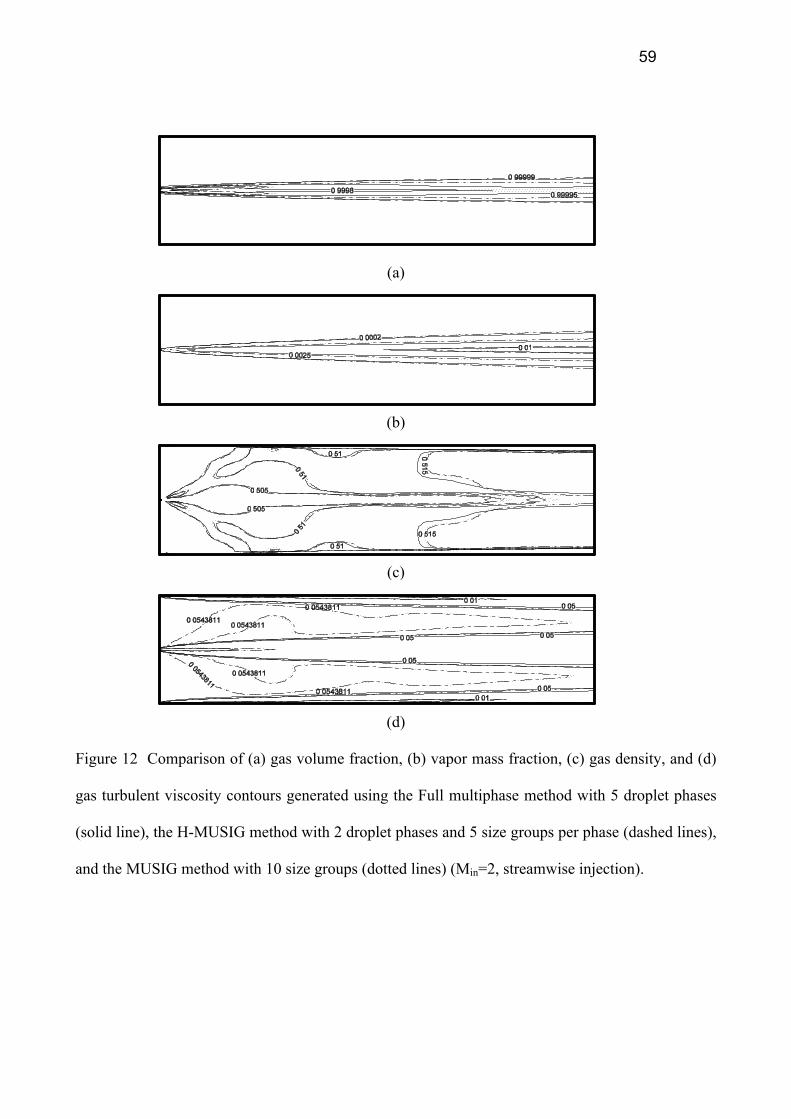
59

0.99999

0.999950.9998

(a)

0.0002

0.0025

0.01

(b)

0.505

0.505

0.51

0.51

0.51

0.51

0.515

0.515

(c)

0.0543811

0.0543811

0.0543811

0.0543811

0.05

0.05

0.05

0.05

0.01

0.01

0.0543811

0.0543811

0.05

(d)




and the MUSIG method with 10 size groups (dotted lines) (Min=2, streamwise injection).

60

800 850 900 950 1000 1050 11000

0.05

0.1

0.15

0.2

0.25

800 850 900 950 1000 1050 11000

0.05

0.1

0.15

0.2

0.25


y(m)

800 850 900 950 1000 1050 11000

0.05

0.1

0.15

0.2

0.25




700 750 800 850 9000

0.05

0.1

0.15

0.2

0.25

700 750 800 850 9000

0.05

0.1

0.15

0.2

0.25

Gas Temperature (K)

y(m)

700 750 800 850 9000

0.05

0.1

0.15

0.2

0.25




(a) (b)

102000 103000 104000 1050000

0.05

0.1

0.15

0.2

0.25

102000 103000 104000 1050000

0.05

0.1

0.15

0.2

0.25

Pressure (Pa)

y(m)

102000 103000 104000 1050000

0.05

0.1

0.15

0.2

0.25




0 0.002 0.004 0.006 0.008 0.01 0.0120

0.05

0.1

0.15

0.2

0.25

0 0.002 0.004 0.006 0.008 0.01 0.0120

0.05

0.1

0.15

0.2

0.25

Vapor Mass Fraction

y(m)

0 0.002 0.004 0.006 0.008 0.01 0.0120

0.05

0.1

0.15

0.2

0.25




(c) (d)


using the full multi-phase, MUSIG, and H-MUSIG methods (Min=2, streamwise injection).

61

(a) (b)

(c) (d)


streamwise direction generated using the full multi-phase, MUSIG, and H-MUSIG methods (Min=2, streamwise injection).

65

20 40 60 80 100 1200

0.05

0.1

0.15

0.2

0.25

20 40 60 80 100 1200

0.05

0.1

0.15

0.2

0.25


y(m)

20 40 60 80 100 1200

0.05

0.1

0.15

0.2

0.25




H-MUSIG (5 droplet phase, 2 groups each)

580 600 620 640 660 680 7000

0.05

0.1

0.15

0.2

0.25

580 600 620 640 660 680 7000

0.05

0.1

0.15

0.2

0.25

Gas Temperature (K)

y(m)

580 600 620 640 660 680 7000

0.05

0.1

0.15

0.2

0.25





(a) (b)

Pressure (Pa)

y(m)

99800 99850 99900 999500

0.05

0.1

0.15

0.2

0.25





Vapor Mass Fraction

y(m)

0 0.01 0.02 0.03 0.04 0.05 0.06 0.070

0.05

0.1

0.15

0.2

0.25





(c) (d)


using the full multi-phase, MUSIG, and H-MUSIG methods (Min=0.2, cross stream injection).

66

(a) (b)

(c) (d)


streamwise direction generated using the full multi-phase, MUSIG, and H-MUSIG methods (Min=0.2, cross stream injection).

67

(a)

(b)

(c)

(d)

(e)

(f)


MUSIG (d, e, in increasing Sauter diameter) and the MUSIG (f) methods for cross stream injection

in a supersonic flow field (Min=2).

68

0.99995

0.99999

0.9998

0.9998

0.99999

0.99995

0.99999

(a)

0.001

0.001

0.002

0.002

0.003

0.003

0.004

0.004

(b)

0.51

0.52

0.520.51

0.53

0.53

0.530.52

0.53

0.53

0.53

0.51

0.52

0.53

0.53

(c)

0.074 0.076 0.074

0.074

0.076

0.076

0.075

0.075

0.075

0.025

0.05

(d)




and the MUSIG method with 10 size groups (dotted lines) (Min=2, cross stream injection).

69

800 850 900 950 1000 1050 11000

0.05

0.1

0.15

0.2

0.25

800 850 900 950 1000 1050 11000

0.05

0.1

0.15

0.2

0.25


y(m)

800 850 900 950 1000 1050 11000

0.05

0.1

0.15

0.2

0.25




700 750 800 850 9000

0.05

0.1

0.15

0.2

0.25

700 750 800 850 9000

0.05

0.1

0.15

0.2

0.25

Gas Temperature (K)

y(m)

700 750 800 850 9000

0.05

0.1

0.15

0.2

0.25




(a) (b)

104000 106000 108000 1100000

0.05

0.1

0.15

0.2

0.25

104000 106000 108000 1100000

0.05

0.1

0.15

0.2

0.25

Pressure (Pa)

y(m)

104000 106000 108000 1100000

0.05

0.1

0.15

0.2

0.25




Vapor Mass Fraction

y(m)

0 0.001 0.002 0.003 0.0040

0.05

0.1

0.15

0.2

0.25




(c) (d)


using the full multi-phase, MUSIG, and H-MUSIG methods (Min=2, cross stream injection).

70

(a) (b)

(c) (d)


streamwise direction generated using the full multi-phase, MUSIG, and H-MUSIG methods (Min=2, cross stream injection).

mixing and evaporation of liquid droplets injected into an ... · mixing and evaporation of liquid...

Documents