mixed oligopoly, foreign firms, and location choice oligopoly, foreign firms, and location choice...
TRANSCRIPT

Mixed Oligopoly, Foreign Firms, and Location Choice∗
Noriaki Matsushima†
Graduate School of Business Administration, Kobe University
and
Toshihiro Matsumura
Institute of Social Science, University of Tokyo
July 11, 2005
Abstract
We investigate a mixed market in which a state-owned, welfare-maximizing public firm
competes against profit-maximizing n domestic private firms and m foreign private firms.
A circular city model with quantity-setting competition is employed. We find that the
equilibrium location pattern depends on m. All private firms agglomerate in the unique
equilibrium if m is zero or one. Two foreign firms induce differentiation between domestic
and foreign private firms. More than two foreign firms yield differentiation among foreign
firms. Regardless of n and m, the agglomeration of all domestic private firms appears in
equilibrium. We provide several conditions in which eliminating the public firm from the
market enhances social welfare.
JEL classification numbers: H42, L13, R32
Key words: spatial agglomeration, shipping model, foreign firms, herd behavior
∗ We are grateful to Masahiro Ashiya, Shingo Ishiguro and participants in the seminars at Institute of Statis-
tical Research, University of Tokyo, and Japanese Economic Association Annual Meeting 2003 for their helpful
comments and suggestions. We are also indebted to the Editor Richard Arnott and anonymous referees for their
valuable and constructive suggestions. Needless to say, we are responsible for any remaining errors. Finan-
cial supports of the Grant-in-Aid from Zengin Foundation for Studies on Economics and Finance and from the
Japanese Ministry of Education, Science and Culture, and of ISS Comparative Regionalism Project (CREP) are
greatly appreciated.† Correspondence author: Noriaki Matsushima, Graduate School of Business Administration, Kobe University,
Rokkodai 2-1, Nada-Ku, Kobe, Hyogo 657-8501, Japan. Phone: +81-78-803-6981. E-mail: nmatsush@kobe-
u.ac.jp
1
1 Introduction
Studies of mixed markets, in which state-owned welfare-maximizing public firms compete against
profit-maximizing private firms, have become increasingly popular in recent years.1 Mixed
oligopolies are common in developed, developing, and former communist transitional economies.2
In Japan, in particular, competition between private and public firms exists in many oligopolistic
markets, such as those for banking services, housing loans, life insurance, broadcasting services,
and overnight deliveries.3
In many of these mixed markets, it is often the case that private firms adopt very similar
strategies, exhibiting “herd behavior” that differs from that of public firms. The herd behavior
exhibited by Japanese city banks is a typical example. In this market, private banks compete
domestically against strong public banks, such as the Postal Bank and the Public House Loan
Corporation. Accordingly, many of these private banks rush into the international financial
markets to avoid domestic competition.4
Most existing works on mixed oligopoly, as well as our earlier work, investigate the competi-
tion between public and domestic private firms. In real world economies, however, competitors
of public firms are not limited to domestic private firms. For example, the New Zealand gov-
ernment set up a state-owned public bank to compete against private foreign banks. Similarly,
when the government of Brazil bargained with the Swiss medical company Roche, it used a
public medical institution as a potential competitor in the domestic market. Electricite de
France and Gas de France also compete against foreign private firms in the EU energy markets.
Recently, many foreign private financial institutions rushed into the Japanese financial markets,
which are typical mixed markets, as discussed above. Airline, telecommunication, natural gas,1 For pioneering work on mixed oligopolies, see Merrill and Schneider (1966). See Bos (1986, 1991), Vickers
and Yarrow (1988), and Nett (1993) for excellent surveys.
2 The interest in mixed oligopolies is due to their importance to the economies of Europe, Canada, and Japan
more than to that of the US. However, there are examples of mixed oligopolies in the US, such as the packaging
and overnight-delivery industries.
3 See, e.g., Ide and Hayashi (1992).
4 Several examples of herd behavior are described in Matsushima and Matsumura (2003).
2
electric power, automobile, and steel industries in many developed and developing countries
are also typical examples. Recently, literature on mixed oligopoly with foreign competitors
has begun to appear, including Fjell and Pal (1996), Pal and White (1998), and Matsumura
(2003a). All of these studies indicate that the existence of foreign competitors (even a single
one) drastically changes the equilibrium outcomes.
In this paper, we also consider foreign competitors explicitly and investigate how the pres-
ence of foreign competitors affects the “herd behavior” in mixed oligopolies. We again use a
location model with a circular city in which firms deliver goods (shipping model).5 We find
that the number of foreign firms substantially affects the equilibrium location patterns. If the
number of foreign competitors is zero or one, the equilibrium location pattern is unique, and
all private firms (both domestic and foreign) agglomerate at the side of the circle opposite the
location of the public firm. In other words, a single foreign firm does not affect the equilibrium
locational choices of private firms. However, if the number of foreign firms is two, multiple
equilibria appear. In every equilibrium, each domestic private firm inevitably changes its lo-
cation, while it is possible that two foreign private firms still locate at the side of the circle
opposite the location of the public firm. If the number of foreign private firms is more than
two, the agglomeration of foreign firms never appears in equilibrium. In other words, more than
two foreign firms yield differentiation among foreign firms. Regardless of the number of foreign
private firms and that of domestic private firms, it is possible that all domestic private firms
agglomerate at one point, although the point of agglomeration depends on the number of foreign
firms. These results then indicate that when the number of foreign firms is relatively small,
the effects on the locational choices by domestic firms are limited. An increase in the number
of foreign firms causes a change of locational choice by domestic private firms, and a further
increase yields diversification among foreign private firms, while it is possible for diversification
among domestic private firms to be limited (herd behavior).5 For discussions on mixed oligopoly with spatial competition, see Cremer, Marchand, and Thisse (1991),
Matsumura and Matsushima (2003, 2004), and Nilssen and Sørgard (2002). For applications of circular-city
shipping Cournot models see, for example, Matsushima (2001) and Matsumura (2003b).
3
In this paper, we use spatial price discrimination models with Cournot competition. Hamil-
ton, Thisse, and Weskamp (1989) and Anderson and Neven (1991) have carried out pioneering
work on location models with quantity competition.6 In a spatial price discrimination model,
we can interpret “space” as product variety and each firm’s location as its most efficient sector.
We can also interpret distant locations from a firm as inefficient sectors of the firm. For exam-
ple, in the automobile industry, “space” represents car size, and a firm’s location indicates that
the firm produces small cars efficiently but produces large cars inefficiently. This interpretation
is similar to those of Eaton and Schmitt (1994) and Norman and Thisse (1999). To explain
flexible manufacturing systems (FMS), they use spatial price discrimination models.
Following this interpretation, our model is applicable to the analysis of mixed markets, where
multi-product firms face Cournot competition. The European automobile industry is a typical
example of such mixed markets. Most automobile enterprises are multi-product firms. Several
automobile manufacturers are state ownership companies. Renault is a partially state-owned
company, and Volkswagen is also owned by the government of Lower Saxony, which owns a 20%
stake in the firm. Most economists describe the competition in the automobile industry using
Cournot models. The airline industry is another typical example. In this industry, there were
(and still are) state-owned airline companies, such as Air France. Airline companies are also
multi-product (multi-market) firms, and there are papers treating airline companies as multi-
product firms (e.g., Borenstein (1991) and Gimeno (1999)). The market structure of airline
industry is reasonably consistent with a Cournot model, where firms commit to quantities and
then prices adjust along the reaction curves. The Cournot assumption is common to most
empirical studies on the airline industry (e.g., Reiss and Spiller (1989) and Richard (2003)).
The remainder of this paper is organized as follows. In Section 2, we present the basic
model. In Section 3, we investigate the equilibrium outcomes of the model. Section 4 discusses
welfare implications. Section 5 extends the basic model and investigate three issues that are6 Greenhut and Greenhut (1975) and Norman (1981) have already examined Cournot competition in spatial
models, but they discussed the equilibrium price pattern rather than the equilibrium pattern of location. Recently,
the literature on location-quantity models has become richer and more diverse. For example, Chamorro-Rivas
(2000) and Pal and Sarkar (2002) consider spatial Cournot competition among multi-plant firms.
4
ignored in the basic analysis. Section 6 concludes the paper.
2 The model
We formulate an oligopoly model in a mixed market, in which a welfare-maximizing public
firm competes against profit-maximizing domestic private firms and foreign private firms. Firm
0 is the public firm, and there exist n domestic private firms (firm 1, firm 2,..., firm n) and
m foreign private firms.7 Let D ≡ {1, 2, ..., n} denote the set of domestic private firms and
F ≡ {n + 1, n + 2, ..., n + m} denote the set of foreign private firms.
We now present a two-stage location-quantity game. The basic structure of the model is
from Pal (1998a). Let xi (i ∈ {0, 1, . . . , n + m}) be the locations of firm i. xi is the point on
the circle located at a distance from 0 (measured clockwise).
In the first stage, firm 0 locates at a point on the circle. Without loss of generality, we assume
that firm 0 locates at x0 = 0. Later, each private firm i (i ∈ {1, . . . , n + m}) simultaneously
chooses its location xi. Let qi(x) denote the firm i’s output offered at each point x ∈ [0, 1]. x is
the point on the circle located at a distance from 0 (measured clockwise). In the second stage,
each firm i (i ∈ {0, . . . , n + m}) observes its competitors’ locations and simultaneously chooses
qi(x) ∈ [0,∞) for x ∈ [0, 1]. Let p(x) denote the price of the product at x and
q(x) ≡n+m∑i=0
qi(x)
denote the total quantity supplied at x. We assume that the demand function at each point x
is linear and is given by:
p(x) = a − bq(x),
where a and b are positive constants. Let d(x, xi) denote the distance between x and xi.7 In this paper, the government is not permitted to nationalize more than one firm. As pointed out by Merrill
and Schneider (1966), the most efficient outcome is achieved by the nationalization of all firms, if nationalization
does not change the costs of firms (i.e., no X-inefficiency in the public firm exists). The need for the analysis
of a mixed oligopoly lies in the fact that it is impossible or undesirable, for political or economic reasons, to
nationalize an entire sector. For example, without competitors, public firms may lose the incentive to improve
their costs, resulting in a loss of social welfare. Thus, we do not consider the possibility of nationalizing all firms.
5
This signifies the shorter distance of the two possible ways to transfer the goods along the
perimeter. To ship a unit of the product from its own location to a consumer at point x, each
firm i (i ∈ {0, . . . , n+m}) pays a transport cost td(x, xi), where t is a constant value. Firms are
able to discriminate among consumers since they control transportation. Consumer arbitrage
is assumed to be prohibitively costly.8 Each of (n + m + 1) firms has identical technology
and constant marginal cost of production, which is normalized to zero. These assumptions are
standard and also made in many other location–quantity models.
3 Equilibrium
In this section, we discuss the equilibrium in the model formulated above. We use subgame
perfection as the equilibrium concept. The game is solved by backward induction. First, we
discuss the equilibrium outcomes in the second-stage subgames given the location of each firm.
3.1 Quantity choice
We follow the Cournot assumption that firms compete in quantities at each point in the market.
Since marginal production costs are constant, quantities set at different points by the same firm
are strategically independent. Cournot equilibria can be characterized by a set of independent
Cournot equilibria, one for each point x. Let πi(x) denote firm i’s (i ∈ {1, . . . , n + m}) profit
at x, given the locations of all firms;
πi(x) = (a − bq(x) − t(d(x, xi))) qi(x). (1)
Let w(x) denote the domestic social surplus (consumer surplus plus profits of all domestic firms)
at x.
w(x) =∫ q(x)
0(a − bm)dm − q(x)(a − bq(x)) +
n∑i=0
(a − bq(x) − td(x, xi))qi(x). (2)
8 This assumption is not essential. Unless transportation costs for consumers are strictly smaller than those
of firms, consumer arbitrage plays no role in our model. For this discussion, see Hamilton, Thisse, and Weskamp
(1989).
6
The first-order condition of firm 0 and firm i (i ∈ {1, . . . , n + m}) is given, respectively, by
a − td(x, x0) − bq0(x) − bn∑
i=1
qi(x) = 0, (3)
a − td(x, xi) − bqi(x) − bn+m∑i=0
qi(x) = 0. (4)
In this paper, we assume that the whole market will always be served by firm 0. This assumption
is satisfied if 2a ≥ t(n + 1).9
We first show that the output level of all domestic firms (both public and private) does not
depend on the locations of domestic private firms.
Lemma 1 (i) q0 +∑
i∈D qi does not depend on xi ∈ D. (ii) For any i ∈ D ∪ F , qi(x) = 0 if
d(x, x0) ≤ d(x, xi).
Proof: See Appendix.
We explain Lemma 1(i) intuitively. Let R0(q1, q2, ..., qn+m+1) denote the reaction function
of firm 0 in the second-stage game. From (3), we have ∂R0/∂qi = −1 for all i ∈ D. In other
words, one unit reduction of firm i’s output (i ∈ D) increases the best output of firm 0 by
one unit. xi affects the marginal cost of firm i for each market x and may therefore affect the
equilibrium qi(x). However, this effect is offset by the behavior of firm 0, so the output level of
all domestic firms does not depend on xi (i ∈ D). Since the total output level of all firms other
than firm j (j ∈ F ) does not depend on xi (i ∈ D), xi never affects the output of each foreign
firm.
On the other hand, the locations of foreign firms affect the total output, so they also affect
the profits of all firms. Let F (x) and m(x) denote the set of foreign firms supplying at market
x and the number of such firms, respectively, The total quantity supplied and the price are:
q(x) =
(m(x) + 1)a − td(x, x0) −∑
j∈F (x)
td(x, xj)
(m(x) + 1)b, (5)
9 A similar assumption (sufficiently large a) is also made in many studies of mixed oligopoly and quantity-
setting spatial models. See, among others, Anderson and Neven (1991) and Pal (1998a).
7
p(x) =
td(x, x0) +∑
j∈F (x)
td(x, xj)
(m(x) + 1). (6)
The output quantity and profit of firm i supplying for market x are given by
qi(x) =
td(x, x0) +∑
j∈F (x)
td(x, xj) − (m(x) + 1)td(x, xi)
(m(x) + 1)b, (7)
πi(x) =
⎡⎢⎣td(x, x0) +
∑j∈F (x)
td(x, xj) − (m(x) + 1)td(x, xi)
⎤⎥⎦
2
(m(x) + 1)2b. (8)
If firm i does not supply for market x (i.e., (7) is non-positive), its profit from market x is zero.
From (8), we obtain the following Lemma.
Lemma 2 The profits of firm i ∈ D ∪ F do not depend on xj if j = i and j ∈ D.
A foreign firm j supplies for market x only if d(x, x0) ≥ d(x, xj). p(x) in (6) is smaller than
or equal to td(x, x0) (the price in which foreign firms do not enter). Therefore, we have the
following Lemma.
Lemma 3 Suppose that foreign firms supply at x. The price at x, p(x), is smaller than that
in which foreign firms do not enter. In other word, consumer surplus at x is higher than that
in which foreign firms do not enter.
3.2 Location choice
In this subsection, the equilibrium locations are discussed. First, we present a result describing
the equilibrium location without foreign private firms as a benchmark.
Result (Matsushima and Matsumura (2003)) If m = 0, in the unique equilibrium, all
private firms agglomerate at 1/2 (the side of the circle opposite the location of the public firm).
The intuition behind this result is as follows. If m = 0, the price at market x is td(x, x0) (see
(6)), that is, the price at each local market is equal to the unit transportation cost of the public
8

firm. The further away the public firm is from a market, the higher the public firm’s transport
cost at the market will be. Each private firm faces tough competition from the public firm in the
market nearer the location of the public firm. For each private firm, markets near the location
of the public firm are thin, and those far away from that location are thick. To minimize the
transportation costs at the largest market for private firms, each firm prefers the location that
is farthest from the public firm. This produces an agglomeration of private firms.
We now discuss the equilibrium location patterns with foreign private firms. Lemma 2
states that the location of each domestic private firm does not affect the profits of other firms
at all. This implies that none of the firms needs to worry about where the domestic private
firms locate. Thus, each domestic private firm can choose its location without considering its
strategic effect. Under these conditions, if one point is the best location for a domestic private
firm, then it is also the best location for all other domestic firms. Thus, the agglomeration of
all domestic private firms can always appear in equilibrium.
Proposition 1 At least one equilibrium exists in which all domestic private firms agglomerate
at one point.
Proof: See Appendix.
However, this property does not hold true for foreign firms. The location of one foreign firm
does affect the output choice of all other foreign firms; thus, the location choices made by a
foreign firm have a strategic effect. Owing to this strategic interaction, the optimal location of
one foreign firm depends on the locations of other foreign firms.
Proposition 2 Suppose that m = 1. In the unique equilibrium xi = 1/2 for all i ∈ D ∪ F.
Proof: See Appendix.
Proposition 2 indicates that agglomeration of all private firms still appears even after one foreign
firm enters the market. This result, however, does not hold true if there are two or more foreign
firms. Proposition 3 indicates that two foreign firms yield a differentiation between foreign and
domestic private firms, although it is possible that two foreign firms still locate at the side of
9
the circle opposite the location of the public firm. Proposition 4 states that more than two
foreign firms yield differentiation among foreign firms.
Proposition 3 Suppose that m = 2. (i) The following location choices constitute an equilib-
rium: each domestic private firm i chooses either xi = 5−√3
11 ∼ 0.297 or xi = 6+√
311 ∼ 0.703,
and each foreign firm j chooses xj = 1/2. (ii) The following location choices also consti-
tute an equilibrium: each domestic private firm i chooses either xi = 18−√66
30 ∼ 0.329 or
xi = 12+√
6630 ∼ 0.671, one foreign firm j chooses xj = 13/30 and the other foreign firm k
chooses xk = 17/30.
Proof: See Appendix.
Proposition 4 Suppose that m > 2. The agglomeration of all foreign firms never appears in
equilibrium.
Proof: See Appendix.
We explain the intuition behind Propositions 2–4. Suppose that all private firms locate at
the point 1/2. We consider whether or not each private firm has an incentive for deviating this
location strategy, given the other firms’ location.
From (8), we can assume that the markets near 0 (the location of the public firm) are not
profitable, since td(x, x0) is small. In other words, the markets near 0 are not profitable for
each private firm; thus, there is a strong incentive to avoid this severe competition against the
public firm. As a result, a private firm chooses the furthest location from the public firm. This
mechanism is in common with Matsushima and Matsumura (2003). This is called the “public
firm effect.” At the same time, the markets near 1/2 (the location of the foreign firms) are not
profitable, since m = m for the markets near point 1/2 (we have defined m as the number of
supplying foreign firms). Thus, each firm has an incentive to be far away from point 1/2. This
is called the “foreign firm effect.” An increase in m accelerates the competition and reduces
the prices at the markets near 1/2. Therefore, the foreign firm effect depends on m.
Then, given the locations of all other firms, one firm (firm k) deviates and slightly reduces
xk from 1/2. This reduces the distance from the location of the public firm and increases the
10
distance from the locations of foreign firms. If the foreign firm effect dominates the public firm
effect, it increases the profits of firm k. The foreign firm effect is increasing in the number of
foreign firms other than firm k; thus, there naturally exists a threshold value dominating the
public firm effect. In our model, this threshold value is two. If the number of other foreign
firms is two or more, firm k has the above-mentioned deviation incentive.
The number of foreign firms other than itself locating at 1/2 is m for each domestic private
firm and m − 1 for each foreign firm. Suppose that m = 1. The number of foreign firms other
than itself locating at 1/2 is 0 or 1 for all private firms and the public firm effect dominates
the foreign firm effect. This is the reason why all private firms agglomerate at 1/2 when m = 1
(Proposition 2). Suppose that m = 2. The number of foreign firms other than itself locating
at 1/2 is 1 for foreign firms and 2 for domestic firms. Thus, the public firm effect dominates
the foreign firm effect for each foreign firm, but the foreign firm effect dominates the public
firm effect for each domestic private firm. This is the reason why domestic private firms do
not chooses the location 1/2, while two foreign firms choose it (Proposition 3(i)). Suppose that
m ≥ 3. The number of foreign firms other than itself locating at 1/2 is 2 or more for all private
firms, and the foreign firm effect dominates the public firm effect. Thus, there is no equilibrium
where m foreign firms locate at 1/2 (Proposition 4).
We now mention the difference between the location patterns of Proposition 3(i) and 3(ii).
Consider the two-foreign-firm case. We denote one foreign firm as “firm a” and the other as
“firm b.” Proposition 3(i) states that firm a’s optimal location is 1/2 when xb = 1/2, and
Proposition 3(ii) states that it is 13/30 when xb = 17/30. This implies that an increase in
the distance between firm b’s location and the public firm’s enlarges firm a’s optimal distance
from the public firm’s location. We explain the reason behind this strategic complementarity.
Suppose that xb = 17/30. Firm a chooses its location which balances the public firm and the
foreign firm effects, and it is 13/30. Suppose that firm b moves from 17/30 to 1/2. The move
enhances the public firm effect at market 13/30 because the move reduces firm b’s cost for
market 13/30 and induces the larger output of the public firm. Since the move strengthens the
11
public firm effect, firm a has a higher incentive for moving away from the public firm. As a
result, firm a’s optimal location becomes 1/2. In short, a longer distance between firm b and
the public firm yields the longer optimal distance between firm a and the public firm. This
strategic complementarity yields multiple equilibria.
Proposition 4 presents a property of equilibrium location but does not fully describe the
equilibrium location pattern when m ≥ 3. Since foreign firms never agglomerate at 1/2 in
equilibrium, the asymmetries between foreign firms inevitably arise. For example, the distance
between each foreign firm and the public firm never becomes the same across all foreign firms.
Thus, as opposed to the case without foreign firms, it is impossible to solve the m-foreign firm
case systematically. Although we can solve each of the problems in the case where m = 3, m =
4, m = 5, .., in the interests of brevity we only present the results of a 3-foreign-firm case.10
Proposition 5 Suppose that m = 3. The following location choices constitute an equilibrium:
each domestic private firm i chooses either xi = 9216√
2−103915750 ∼ 0.460 or xi = 16141−9216
√2
5750 ∼0.540, and the foreign firms choose xa = 3−√
24 ∼ 0.396, xb = 1/2, and xc = 1+
√2
4 ∼ 0.604,
respectively.
4 Welfare implication
Given that n domestic private firms exist, we compare domestic welfare among four cases: (1)
no foreign firm exists (SW0); (2) one foreign firm exists (SW1); (3) two foreign firms exist, and
they locate at x = 1/2 (SW2a); and (4) two foreign firms exist, and each of them locates at
x = 13/30 and x = 17/30 (SW2b).
4.1 No foreign firm
We first consider the case in which no foreign firm exists. In this case, the public firm’s profit is
zero. Social welfare (SW0) is the consumers’ surplus (CS0) plus the sum of each private firm’s10 The proof is available from the authors on request.
12

profit (Π0).
CS0 = 2∫ 1
2
0
b
2
(a − p(x)
b
)2
dx = 2∫ 1
2
0
b
2
(a − tx
b
)2
dx =12a2 − 6at + t2
24b,
Π0 = 2n
∫ 12
14
(tx − t(1/2 − x))2
bdx =
nt2
24b,
SW0 =12a2 − 6at + (n + 1)t2
24b.
4.2 One foreign firm
We next consider the case in which one foreign firm exists. In this instance, the profit of the
public firm is negative. Social welfare (SW1) is the consumers’ surplus (CS1) plus the profit of
the public firm (π01) plus the sum of each private firm’s profit (Π1).
In this case, the foreign firm locates at x = 1/2 (see Proposition 2). From the proof of
Proposition 2, we find that the foreign firm supplies at x ∈ [1/4, 3/4] (see the last paragraph
before equation (21)).
First, we calculate CS1. The consumers’ surplus at x is bq(x)2/2. From (5) and (6), we find
that this is equal to (a− p(x))2/2b. From (6), the price at x is (by symmetry, we only consider
the range [0, 1/2]):
p(x) =
{tx if x ∈ [0, 1/4],t/4 if x ∈ [1/4, 1/2].
(9)
CS1 = 2∫ 1
2
0
(a − p(x))2
2bdx =
24a2 − 9at + t2
48b.
Next, we calculate π01. From (3), we obtain
q0(x) =a − td(x, x0)
b−∑i∈D
qi(x). (10)
From (7) and proof of Proposition 2 (see the first paragraph after (26)), we have
qi(x) =
{0 if x ∈ [0, 1/4],t(2x−1/2)
2b if x ∈ [1/4, 1/2].(11)
π01 = 2∫ 1
2
0(p(x) − td(x, x0))q0(x)dx = − t(12a − (5 + 2n)t)
192b.
13

Finally, we calculate Π1. Π1 is n times of each domestic private firm’s profit. From (27), we
obtain the profit of each domestic firm and the total profit:
Π1 =n(16(1/2)3 − 24(1/2)2 + 12(1/2) − 1)t2
96b=
nt2
96b.
We have social welfare:
SW1 = CS1 + π01 + Π1 =96a2 − 48at + (9 + 4n)t2
192b.
4.3 Two foreign firms
Third, we consider the case in which one foreign firm exists. In this case, the profit of the public
firm is negative. Social welfare (SW2) is the consumers’ surplus (CS2) plus the profit of the
public firm (π02) plus the sum of each private firm’s profit (Π2).
In this instance, two equilibrium outcomes exist: (a) foreign firms locate at x = 1/2, and
each domestic firm locates at za ≡ (5 − √3)/11 (or (6 +
√3)/11); (b) foreign firms locate at
x = 13/30 and x = 17/30 respectively, and each domestic firm locates at zb ≡ (18 − √66)/30
(or (12 +√
66)/30).
Case (a): From the proof of Proposition 3(i), we find that both foreign firms supply at
x ∈ [1/2, 3/4] (see the last paragraph before Equation (34)).
First we calculate CS2a. As mentioned earlier, consumers’ surplus at x is (a − p(x))2/2b.
From (6), we have
p(x) =
{tx if x ∈ [0, 1/4],t(1 − x)/3 if x ∈ (1/4, 1/2].
(12)
CS2a = 2∫ 1
2
0
(a − p(x))2
2bdx =
216a2 − 72at + 7t2
432b.
Next, we calculate π02a. From (7) and the proof of Proposition 3(i) (see the last paragraph
before Equation (39)), we have
qi(x) =
⎧⎪⎪⎪⎪⎪⎪⎨⎪⎪⎪⎪⎪⎪⎩
0 if x ∈ [0, za/2],t(2x−za)
b if x ∈ [za/2, 1/4],t(1+2x−3za)
3b if x ∈ [1/4, za],t(1−4x+3za)
3b if x ∈ [za, (1 + 3za)/4],0 if x ∈ [(1 + 3za)/4, 1/2] ∪ [1/2, 1],
14

π02a =∫ 1
0(p(x) − td(x, x0))q0(x)dx = − t(15972a − (6655 + (1035 − 240
√3)n)t)
191664b.
Finally, we calculate Π2a. Π2a is n times each domestic private firm’s profit. From (39), we
obtain the profit of each domestic firm and the total profit:
Π2a =n(22z3
a − 30z2a + 12za − 1)t2
72b=
n(13 + 4√
3)t2
2904b.
SW2a = CS2a + π02a + Π2a =287496a2 − 143748at + (29282 + (5679 + 72
√3)n)t2
574992b.
Case (b): From the proof of Proposition 3(ii), we find that the foreign firm located at x =
13/30 supplies at x ∈ [13/60, 13/20] and that located at x = 17/30 supplies at x ∈ [7/20, 47/60]
(see item “(4) x2 ∈ (17/45, 1/2]” in the proof of Proposition 3(ii)).
First, we calculate CS2b. As mentioned earlier, consumers’ surplus at x is (a − p(x))2/2b.
From (6), we have
p(x) =
⎧⎪⎪⎪⎨⎪⎪⎪⎩
tx if x ∈ [0, 13/60],13t/60 if x ∈ [13/60, 7/20],t(1 − x)/3 if x ∈ [7/20, 13/30],t(15x + 2)/45 if x ∈ [13/30, 1/2].
(13)
CS2b = 2∫ 1
2
0
(a − p(x))2
2bdx =
48600a2 − 16056at + 1531t2
97200b.
Next, we calculate π02b. From (7) and the proof of Proposition 3(ii) (see item “(5) x1 ∈(13/45, 7/20]” in the proof of Proposition 3(ii)), we have
qi(x) =
⎧⎪⎪⎪⎪⎪⎪⎪⎪⎪⎪⎪⎪⎪⎪⎨⎪⎪⎪⎪⎪⎪⎪⎪⎪⎪⎪⎪⎪⎪⎩
0 if x ∈ [0, zb/2],t(2x−zb)
b if x ∈ [zb/2, 13/60],t(13/30+2x−2zb)
2b if x ∈ [13/60, zb],t(13/30−2x+2zb)
2b if x ∈ [zb, 7/20],t(1−4x+3zb)
3b if x ∈ [7/20, 13/30],t(2/15−2x+3zb)
3b if x ∈ [13/30, 1/2],t(17/15−4x+3zb)
3b if x ∈ [1/2, (17 + 45zb)/60],0 if x ∈ [(17 + 45zb)/60, 1],
π02b =∫ 1
0(p(x) − td(x, x0))q0(x)dx = − t(494640a − (201300 − (103655 − 16389
√66)n)t)
5832000b.
15

Finally, we calculate Π2b. Π2b is n times each domestic private firm’s profit. From (60), we
obtain the profit of each domestic firm and the total profit:
Π2b =n(243000z3
b − 437400z2b + 208980zb − 12269)t2
2916000b=
n(8143 + 1188√
66)t2
2916000b.
We summarize them:
SW2b = CS2b + π02b + Π2b =972000a2 − 486000at + (97720 − (29123 − 6255
√66)n)t2
1944000b.
4.4 Comparison
Given that n domestic private firms exist, we compare four cases: (1) no foreign firm exists
(SW0), (2) one foreign firm exists (SW1), (3) two foreign firms exist, and they locate at x = 1/2
(SW2a), (4) two foreign firms exist, and they locate at x = 13/30 and x = 17/30 (SW2a).
First, we compare SW2b with SW2a. We obtain
SW2b − SW2a =(−1703680 + (8325405
√66 − 324000
√3 − 64318213)n)t2
2587464000b,
and it is positive for any n ≥ 1. This implies the following proposition.
Proposition 6 (i) SW2b < SW2a if n = 0, and (ii) SW2b > SW2a for any n ≥ 1.
The differentiation between two foreign firms yields larger welfare than the agglomeration of
them if domestic firms exist. On the other hand, if no domestic private firm exists, agglomeration
of foreign firms is better for domestic welfare.
Suppose that there is no domestic private firm. The cost of the public firm, which is the sole
domestic supplier, is highest at the market 1/2. Thus, the increase of the supply for the market
1/2 improves welfare most efficiently. Suppose that a foreign domestic firm a locates at point
y < 1/2 and the other foreign firm b locates at point 1 − y. Suppose that both firms relocate,
one at point y′(y < y′ ≤ 1/2) and the other at point 1− y′. We can show that the total output
for market x (y′ ≤ x ≤ 1 − y′) increases, while that for the other market remains unchanged
as long as both firms provide a supply. Since the relocation increases the total output and,
16
thus, consumer surplus for market 1/2, it improves domestic welfare. Thus, the agglomeration
of foreign firms improves domestic welfare.
Suppose that domestic private firms exist. As mentioned above, the agglomeration of foreign
firms yields a higher total output of foreign firms, resulting in the profit transfer from domestic
firms to foreign firms. It reduces the profits of domestic private firms and total social domestic
surplus.
Next, we compare SW0, SW1, and SW2b. We obtain
SW0 − SW1 =(−1 + 4n)t2
192b, SW0 − SW2b =
(−16720 + (110123 − 6255√
66)n)t2
1944000b.
These two differences are positive for any n ≥ 1. We obtain
SW1 − SW2b =(−6595 + (69623 − 6255
√66)n)t2
1944000b,
which is positive for any n ≥ 2. These equations imply the following proposition.
Proposition 7 (i) SW0 < SW1 < SW2b for n = 0, (ii) SW0 ≥ max{SW1, SW2b} for any
n ≥ 1, and (iii) SW1 > SW2b for any n ≥ 2.
Proposition 7 states that an increase in the number of foreign firms improves welfare if no
domestic firm exists. Conversely, if domestic private firms exist, eliminating foreign firms im-
proves welfare. Eliminating foreign firms increases the profits of domestic firms when domestic
private firms exist; thus, it improves domestic welfare. No such effect exists in the case without
domestic private firms, so eliminating foreign firms does not improve welfare.11
To check the efficiency of the locations, we consider the following solution. Suppose that
the social planner cannot control the output of each private firm but can control the locations
of domestic private firms. The following lemma shows that when the number of foreign firms
is zero or one, the location equilibrium is efficient from the viewpoint of social welfare.12
11For a discussion on private duopoly, see Ono (1990).12The proof is available upon a request. The mathematica file is available.
17
Lemma 4 Suppose that the social planner cannot control the output of each private firm but
can control the locations of the domestic private firms. In that case, the social planner chooses
the locations x1 = x2 = . . . = xn = 1/2.
The result is similar to that of Matsushima and Matsumura (2003). In our model, the public
firm is inferior at the market near 1/2 and superior at the market near 0. Thus, additional
production by a private firm greatly improves social welfare at the market near 1/2 but not at
the market near 0. If each private firm locates at 1/2, the additional output is supplied most
intensively at the market where the additional supply has the most value.
As shown in Proposition 3, when there are two foreign firms, domestic private firms do not
agglomerate at 1/2. The location pattern in which two foreign firms exist is inefficient. We can
show that eliminating the public firm may enhance social welfare when there are two foreign
firms.
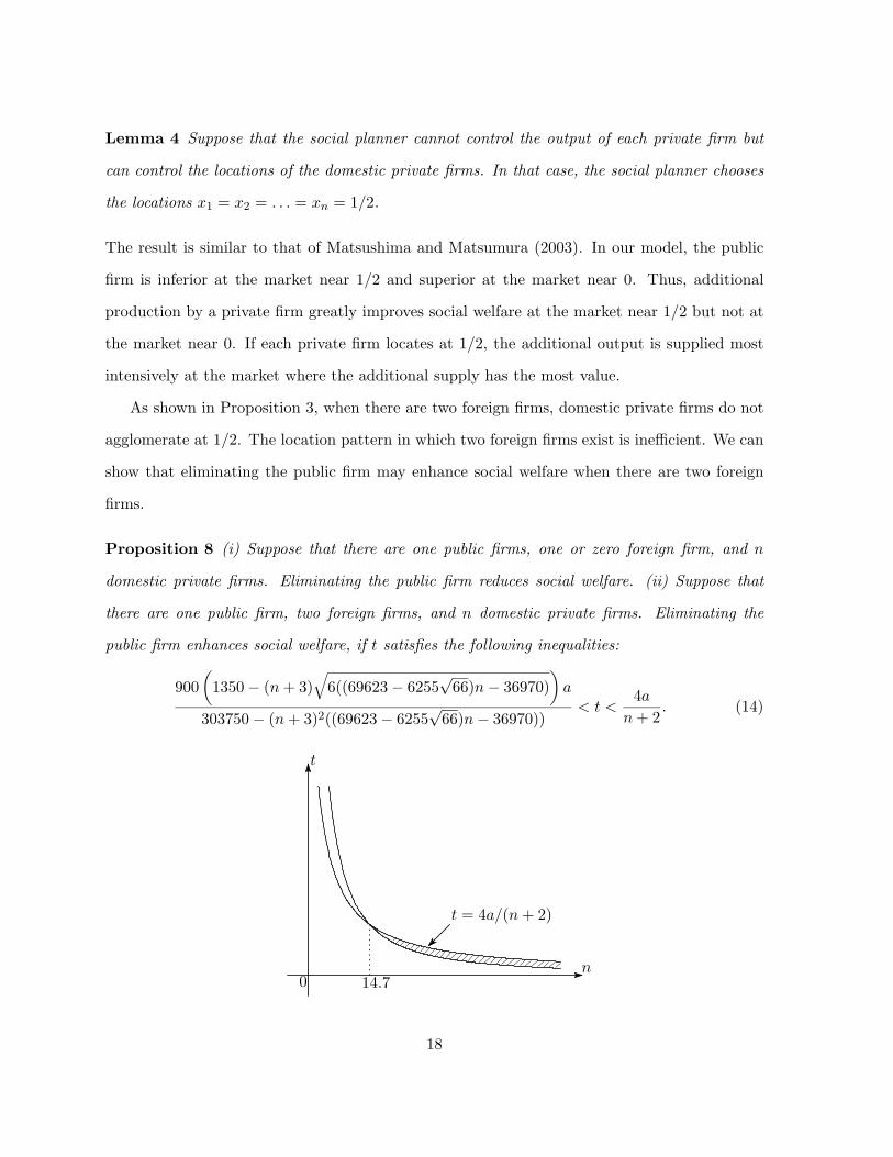
Proposition 8 (i) Suppose that there are one public firms, one or zero foreign firm, and n
domestic private firms. Eliminating the public firm reduces social welfare. (ii) Suppose that
there are one public firm, two foreign firms, and n domestic private firms. Eliminating the
public firm enhances social welfare, if t satisfies the following inequalities:
900(
1350 − (n + 3)√
6((69623 − 6255√
66)n − 36970))
a
303750 − (n + 3)2((69623 − 6255√
66)n − 36970))< t <
4a
n + 2. (14)
14.7n
0
t
t = 4a/(n + 2)
18

When there is only one or zero foreign firms, the locations of domestic private firms are efficient
from the viewpoint of social welfare. On the contrary, when there are two foreign firms, the
locations of domestic private firms are inefficient from the viewpoint of social welfare. As the
transport cost per length increases, the welfare loss induced by the inefficient locations increases.
As the number of domestic private firms increases, the significance of the welfare loss increases.
Therefore, when the above inequalities are satisfied, the public firm harms social welfare.
5 Extensions
In this section, we investigate three problems that have been disregarded in the previous sections.
5.1 Multiple public firms
In the previous sections, we assume that the number of public firms is one. In this section, we
investigate a model with two public firms. We consider the following three stage games: first,
one public firm (firm 0) chooses its location; second, the other public firm (firm 00) chooses its
location after observing firm 0’s location; third, observing the locations of the public firms, each
private firm chooses its location simultaneously; fourth, the firms set the quantities supplied at
each point x ∈ [0, 1]. Without loss of generality, we assume that the public firms locate at xa
and 1 − xa, respectively (xa ∈ [0, 1/4]). In other words, firm 00 chooses the distance between
two public firms, 2xa.
0
1/2
xa1 − xa
1/43/4
5.1.1 No foreign firm
First, we consider the second stage location choices of domestic private firms, given the locations
of the public firms. For the same reason discussed in the previous sections, a private firm’s profit
19
is not affected by the locations of other domestic private firms, and each domestic private firm’s
location choice is strategically independent. Thus, it is sufficient to consider the location of a
domestic private firm.
When a domestic private firm locates at xi ∈ [0, xa], from (8), its profit is:
π =∫ xi
0
(t(xa − m) − t(xi − m))2
bdm +
∫ xi+xa2
xi
(t(xa − m) − t(m − xi))2
bdm
+∫ 1
1+xi+1−xa2
(t(m − (1 − xa)) − t(1 + xi − m))2
bdm =
t2(xa − xi)2(xa + 2xi)3b
.
When xi = 0, π is maximized and then the profit is x3at
2/3b.
When a domestic private firm locates at xi ∈ [xa, 1/2], from (8), the profit of it is:
π =∫ xi
xi+xa2
(t(m − xa) − t(xi − m))2
bdm +
∫ 12
xi
(t(m − xa) − t(m − xi))2
bdm
+∫ 1−xa+xi
2
12
(t(1 − xa − m) − t(m − xi))2
bdm =
t2(xa − xi)2(3 − 2xa − 4xi)6b
.
When xi = 1/2, π is maximized and then the profit is (1/2 − xa)3t2/3b. This profit is larger
than that in which the private firm locates at xi = 0.
Next, we consider the location choices of the public firms in the first and second stages.
Taking subsequent locations of private firms into account, social welfare (consumers’ surplus
plus the sum of the firms’ profits) is given by
SW = 2
(∫ xa
0
(a − t(xa − m))2
2bdm +
∫ 12
xa
(a − t(m − xa))2
2bdm
)+ n × (1/2 − xa)3t2
3b
=12a2 − 6(8x2
a − 4xa + 1)at + (12x2a − 6xa + 1 + n(1 − 2xa)3)t2
24b.
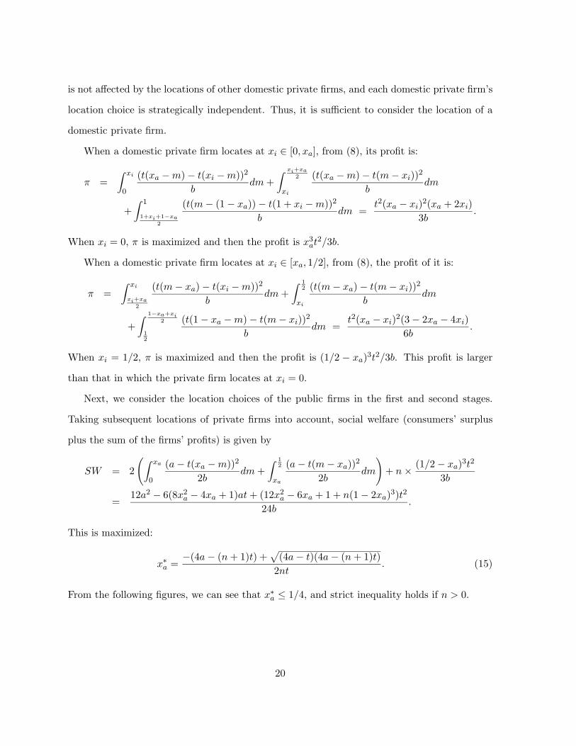
This is maximized:
x∗a =
−(4a − (n + 1)t) +√
(4a − t)(4a − (n + 1)t)2nt
. (15)
From the following figures, we can see that x∗a ≤ 1/4, and strict inequality holds if n > 0.
20
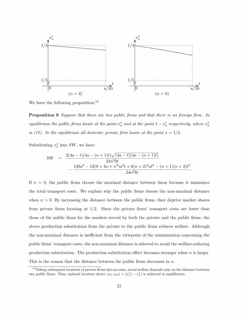
1/4
1/5
1/4
1/5
a/10 a/10tt
(n = 4) (n = 8)
x∗a x∗
a
00
We have the following proposition:13
Proposition 9 Suppose that there are two public firms and that there is no foreign firm. In
equilibrium the public firms locate at the point x∗a and at the point 1− x∗
a respectively, where x∗a
is (15). In the equilibrium all domestic private firm locate at the point x = 1/2.
Substituting x∗a into SW , we have:
SW =2(4a − t)(4a − (n + 1)t)
√(4a − t)(4a − (n + 1)t)
24n2bt
− 128a3 − 12(8 + 4n + n2)a2t + 6(n + 2)2at2 − (n + 1)(n + 2)t3
24n2bt.
If n = 0, the public firms choose the maximal distance between them because it minimizes
the total transport costs. We explain why the public firms choose the non-maximal distance
when n > 0. By increasing the distance between the public firms, they deprive market shares
from private firms locating at 1/2. Since the private firms’ transport costs are lower than
those of the public firms for the markets served by both the private and the public firms, the
above production substitution from the private to the public firms reduces welfare. Although
the non-maximal distance is inefficient from the viewpoint of the minimization concerning the
public firms’ transport costs, the non-maximal distance is selected to avoid the welfare-reducing
production substitution. The production substitution effect becomes stronger when n is larger.
This is the reason that the distance between the public firms decreases in n.13Taking subsequent locations of private firms into account, social welfare depends only on the distance between
two public firms. Thus, optimal location choice (x0, x00) = (x∗a1 − x∗
a) is achieved in equilibrium.
21
5.1.2 One foreign firm
First, we discuss the location of the foreign firm. From (8), we conclude that the profit of the
foreign firm is the quarter of a domestic private firm’s profit function in the former subsection.
Therefore, the location of the foreign firm is identical to that of the domestic firm discussed in
the former subsection. That is, the foreign firm locates at x = 1/2.
Second, we discuss the locations of domestic private firms. As discussed in the former
subsection, on [0, xa], the optimal location of a domestic private firm is x = 0 and then the
profit is x3at
2/3b. On [xa, 1−xa], the foreign firm supplies at x ∈ [(1/2+xa)/2, (1−xa +1/2)/2]
(see, qi(x) in (7)). Given the location of a domestic private firm xi(∈ [xa, 1/2]), we now present
the range in which the domestic private firm supplies a positive amount of goods. From (7), at
m ∈ [1/2, 1 − xa], if the following inequality is satisfied, the quantity supplied by the domestic
private firm is positive:
t(1 − xa − m) + t(m − 1/2) − 2t(m − x)2b
> 0 ⇔ m <1 − 2xa + 4x
4≡ H(xa, x)
(<
1 − xa + 1/22
).
H(xa, x) is larger than 1/2, if and only if x > (1 + 2xa)/4. We have to consider two cases: (i)
x ∈ [xa, (1 + 2xa)/4], (ii) x ∈ [(1 + 2xa)/4, 1/2].
(i) x ∈ [xa, (1 + 2xa)/4]: On [(xa + x)/2, x], the foreign firm does not supply; on [x, (1/2 +
xa)/2], the foreign firm does not supply; on [(1/2 + xa)/2, (1 − 2xa + 4x)/4], the foreign firm
supplies. From (8), the profit of the domestic firm is presented by
∫ x
x+xa2
(t(m − xa) − t(x − m))2
bdm +
∫ 1/2+xa2
x
(t(m − xa) − t(m − x))2
bdm
+∫ 1−2xa+4x
4
1/2+xa2
(t(m − xa) + t(1/2 − m) − 2t(m − x))2
4bdm =
t2(xa − x)2(1 − 2x)4b
.
This is maximized at x = (1 + xa)/3(> (1 + 2xa)/4). That is, the optimal location is the
boundary, x = (1 + 2xa)/4.
(ii) x ∈ [(1 + 2xa)/4, 1/2]: On [(xa + x)/2, (1/2 + xa)/2], the foreign firm does not supply;
on [(1/2+xa)/2, x], the foreign firm supplies; on [x, (1− 2xa +4x)/4], the foreign firm supplies.
22

From (8), the profit of the domestic firm is presented by∫ 1/2+xa
2
x+xa2
(t(m − xa) − t(x − m))2
bdm +
∫ x
1/2+xa2
(t(m − xa) + t(1/2 − xa) − 2t(x − m))2
4bdm
+∫ 1
2
x
(t(m − xa) + t(1/2 − m) − 2t(m − x))2
4bdm
+∫ 1−2xa+4x
4
12
(t(1 − xa − m) + t(m − 1/2) − 2t(m − x))2
4bdm
=t2((1 − 2xa)3 − 2(1 − 2x)3)
96b.
This is maximized at x = 1/2 and then the profit is (1− 2xa)3t2/96b. We find that on [xa, 1/2],
the optimal location of the domestic private firm is x = 1/2.
We have shown that either x = 0 and x = 1/2 is the best for domestic firms. We then
compare the two locations; x = 0 and x = 1/2. The difference between the profits in which the
private firm locates at x = 0 and x = 1/2 is:
(1 − 2xa)3t2
96b− x3
at2
3b=
(1 − 6xa + 12x2a − 40x3
a)t2
96b.
This is positive if and only if xa < xa 0.193, where xa satisfies 1 − 6xa + 12x2a − 40x3
a = 0.
Third, we derive the optimal locations of the public firms. Consumers surplus is given by
CS = 2
(b
2
∫ xa
0
(a − t(xa − m)
b
)2
dm +b
2
∫ 1/2+xa2
xa
(a − t(m − xa)
b
)2
dm
+b
2
∫ 12
1/2+xa2
(2a − t(m − xa) − t(1/2 − m)
2b
)2
dm
)
=24a2 − 3(3 − 12xa + 28x2
a)at + (1 − 6xa + 12x2a + 8x3
a)t2
48b.
When xa > xa, each domestic firm locates at x = 0 and the foreign firm locates at x = 1/2.
The total profits of the public firms are
π0 = 2∫ 1
2
1/2+xa2
(t(m − xa) + t(1/2 − m)
2− t(m − xa)
)× a − t(m − xa)
bdm
= −(1 − 2xa)2t(12a − 5(1 − 2xa)t)192b
.
Social welfare (consumers surplus plus the sum of the domestic firms) is
SW = CS + π0 + nπi
23
=96a2 − 48(1 − 4xa + 8x2
a)at + (9 − 54xa + 108x2a + 8(8n − 1)x3
a)t2
192b.
The first-order condition lead to
xa =32a − 9t − 2
√2(128a2 − 4(8n + 17)at + 9(n + 1)t2)
2(8n − 1)t(>
14).
On [xa, 1/4], the optimal locations of the public firms are xa = 1/4 and 1 − xa = 3/4 and then
SW is
SW =768a2 − 192at + (17 + 8n)t2
1536b. (16)
When xa ≤ xa, each domestic firm locates at x = 1/2 and the foreign firm locates at
x = 1/2. The total profits of the public firms are
π0 = 2∫ 1
2
1/2+xa2
(t(m − xa) + t(1/2 − m)
2− t(m − xa)
)
×(
a − t(m − xa)b
dm − n × t(m − xa) + t(1/2 − m) − 2t(1/2 − m)2b
)
= −(1 − 2xa)2t(12a − 5(1 − 2xa)t − 2n(1 − 2xa)t)192b
.
Social welfare (consumers surplus plus the sum of the domestic firms) is
SW = CS + π0 + nπi
=96a2 − 48(1 − 4xa + 8x2
a)at + (9 + 4n − 6(9 + 4n)xa + 12(9 + 4n)x2a − 8(1 + 4n)x3
a)t2
192b.
The first-order condition lead to
xa =−32a + (9 + 4n)t + 2
√2(128a2 − 4(4n + 17)at + (4n + 9)t2)
2(4n + 1)t.
When this is the interior solution, social surplus is
SW =4(4a − t)(32a − (4n + 9)t)
√2(4a − t)(32a − (4n + 9)t)
24b(4n + 1)2t
− 8192a3 − 12(545 + 136n + 16n2)a2t + 6(17 + 4n)2at2 − (153 + 104n + 16n2)t3
24b(4n + 1)2t.
After tedious calculus, we find that SW in the above equation is smaller than that in which
xa = 1/4. We have the following proposition:
24

Proposition 10 Suppose that there are two public firms and a foreign firm. In equilibrium,
the public firms locate at point 1/4 and at point 3/4, respectively. In equilibrium, all private
firms locate at point 0 and the foreign firm locates at point 1/2.
Propositions 9 and 10 indicate that the equilibrium locations of the public firms depend
on the number of foreign firms. If no foreign firm exists, the public firms choose the non-
maximal distance between them (Proposition 9). We explain why the public firms choose the
maximal location when a foreign firm exists. As noted above, increasing the distance between
the public firms induces production substitution from the private to the public firms. Since
the substitution reduces the foreign firm’s output, it increases the market share of the domestic
firms (public and private) and increases domestic social surplus. This is the reason that the
public firms choose the maximal distance.
5.1.3 Two foreign firms
We investigate the case where two foreign firms exist. We consider two cases: (i) a foreign firm
locates at x ∈ [0, xa] ∪ [1 − xa, 1] and another foreign firm locates at x ∈ [xa, 1 − xa]; (ii) each
foreign firm locates on the range [xa, 1− xa], (note that, we can exclude the case in which each
foreign firm locates on the range [0, xa]∪ [1− xa, 1], because this is inferior to the second case).
In the first case, a foreign firm locates at x = 0 and another foreign firm locates at x = 1/2.
The reason has already been explained in the former subsection.
In the second case, the market structure is similar to that in which a public firm exists on
the circle with length 1 − 2xa.
25
1/2
1/2
0 1
1 − xaxa
h
xa + (1 − 2xa)h
k
1/2 + (1 − 2xa)(k − 1/2)
(h ≤ 1/2) (k ≥ 1/2)0
1/2
1/2
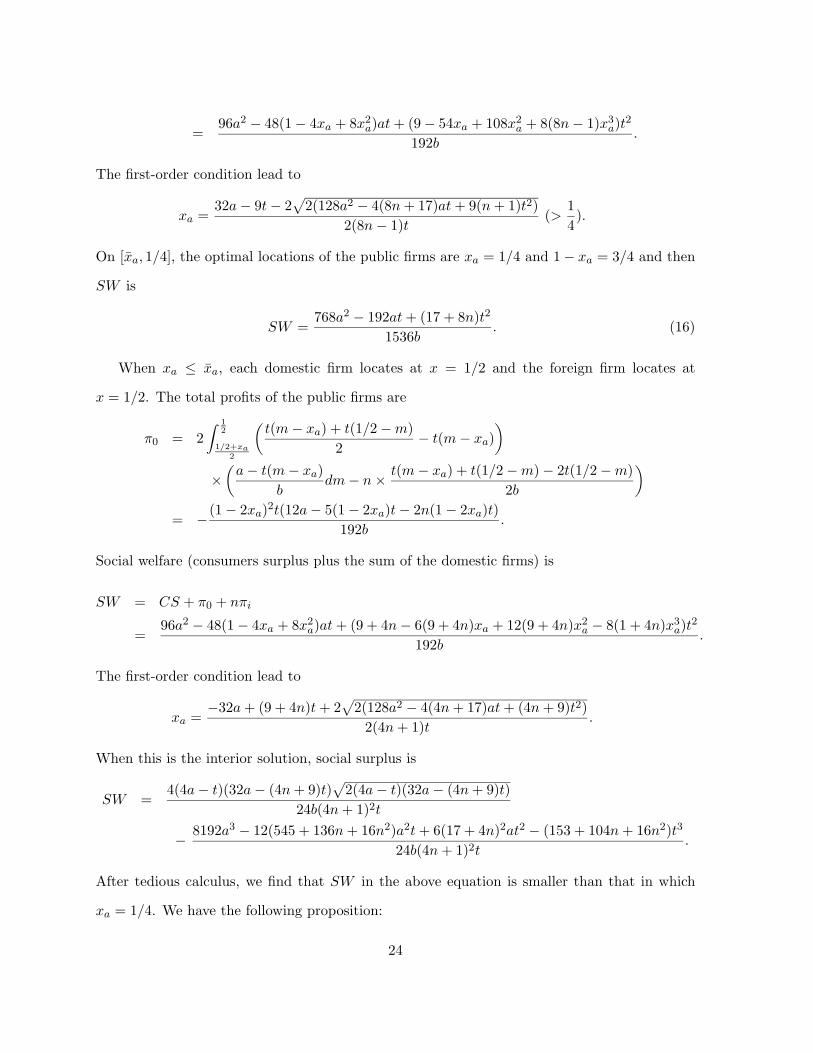
0 xa1 − xa
Therefore, we can use the result (Proposition 3) in section 3: When two foreign firms exist,
each domestic private firm i chooses either xi = 5−√3
11 ∼ 0.297 or xi = 6+√
311 ∼ 0.703, and each
foreign firm j chooses xj = 1/2. The following location choices also constitute an equilibrium:
each domestic private firm i chooses either xi = 18−√66
30 ∼ 0.329 or xi = 12+√
6630 ∼ 0.671, one
foreign firm j chooses xj = 13/30 and the other foreign firm k chooses xk = 17/30. We translate
these location patterns into those which are suitable to the situation considered here.
Lemma 5 Suppose that two foreign firms exist and that each of them locates on the range
[xa, 1 − xa]. (i) Each domestic private firm i chooses either xi = 5−√3+(1+2
√3)xa
11 or xi =6+
√3−(1+2
√3)xa
11 , and each foreign firm j chooses xj = 1/2. (ii) The following location choices
also constitute an equilibrium: each domestic private firm i chooses either xi = 18−√66+2(
√66−3)xa
30
or xi = 12+√
66−2(√
66−3)xa
30 , one foreign firm j chooses xj = (13+4xa)/30 and the other foreign
firm k chooses xk = (17 − 4xa)/30.
In this case, profits of firms are equal to “those in Section 3” times “(1 − 2xa)3. For instance,
if a firm’s profit is 2 in Section 3, the profit in this case is equal to 2 × (1 − 2xa)3. Like a case
with single public firm discussed in Section 3, there are two equilibrium location patterns. We
restrict our attention to the second outcome because the profits of foreign firms are larger than
those in the first outcome.
When the location pattern is the second one in Lemma (one foreign firm j chooses xj =
(13+4xa)/30 and the other foreign firm k chooses xk = (17−4xa)/30.), the profit of a foreign firm
26

is 1369(1− 2xa)3t2/243000b. Given the location pattern, if a foreign firm locates at x = 0, then
it’s profit is (2xa)3/96b. If the former profit is larger than the latter one, this is an equilibrium
outcome. After tedious calculus, we find that if xa < 0.2245 . . ., the second outcome in Lemma
is an equilibrium, but if not, a foreign firm locates at x = 0 and another foreign firm locates at
x = 1/2 in equilibrium. The public firms take the location strategies of foreign firms above into
account and set their locations. Messy calculus, we have the following proposition:
Proposition 11 Suppose that there are two public firms and two foreign firms. Then the
equilibrium locations of the public firms are x∗∗a and 1 − x∗∗
a , where x∗∗a is given by
x∗∗a =
√(32a − 9t)(32a − (4n + 9)t) − (32a − (4n + 9)t)
8nt. (17)
The equilibrium locations of the foreign firms are x = 0 and x = 1/2. The equilibrium location
of each domestic private firm is x = 1/2.
Proposition 11 indicates that the public firms again choose a non-maximal distance between
them. As is shown above, one foreign firm locates at 0 and the other foreign firm locates
at 1/2. Increasing the distance between the public firms has three production substitution
effects. It induces production substitution from all domestic private firms and one foreign firm
locating at 1/2 to the public firms. At the same time, the increase in xa induces production
substitution from the public firms to the other foreign firm locating at 0. The last effect reduces
domestic welfare. On the other hand, when only one foreign firm exists, this effect does not
exist. Thus, the public firms have smaller incentives for increasing their distance, which yields
the non-maximal equilibrium distance.
5.1.4 Welfare implication
When two public firms exist, each one firm locates at a different point. From the equilibrium
locations of public firms, the two yield a larger welfare than one public firm does. The social
planner can locate the public firms at the same point, which yields the same equilibrium welfare
as that in the case of one public firm. Therefore, the additional public firm never reduces social
welfare.
27

As we discuss in Proposition 8, it is possible that no public firm is better than another from
the normative viewpoint. The question then naturally arises of whether no public firm or two
public firms yields a larger welfare. After tedious calculus, we can show that social welfare is
larger in the latter case. However, this result depends on the assumption that public firms are
as efficient as private ones. If we consider the cost differences between public and private firms,
which are discussed in the next subsection, it is possible that this result does not hold.
5.2 Inefficient public firm
In previous sections, we assume that public firms are as efficient as private firms. In this
subsection, we consider a case in which a public firm is less efficient than private firms. We
assume that the marginal cost of the public firm is c > 0, while those of private firms are
normalized to zero.14 We restrict our attention to the case in which no foreign firms exist and
one public firm exists. We also assume that t < 2(a− (n+1)c)/(n+1), which ensures a positive
quantity supplied by the public firm at each point on the circular city.
Without loss of generality, we can assume that x0 = 0. From (8), the profit of a private firm
i locating at xi is given by the following function (note that, at each point, the marginal cost
of the public firm is td(x, x0) + c):
πi =∫ xi
xi2
(tm + c − t(xi − m))2
bdm +
∫ 12
xi
(tm + c − t(m − xi))2
bdm
+∫ 1+xi
2
12
(t(1 − m) + c − t(m − xi))2
bdm
=3c2 + 6ctxi + 3t(t − 2c)x2
i − 4t2x3i
6b.
Differentiating the function with respect to xi, we have:
∂πi
∂xi=
t(1 − 2xi)(c + txi)b
.
It is positive for any xi ∈ [0, 1/2), so the optimal location of each private firm is still 1/2. This
yields the following proposition.14 In this paper, we assume that these costs are given exogenously. For a discussion of endogenous cost
differences, see Corneo and Rob (2003), Ishibashi and Matsumura (2005), Matsumura and Matsushima (2004),
and Nett (1993).
28
Proposition 12 Suppose that there are one public firm, m domestic private firms and no
foreign firm. Suppose that t < 2(a − (n + 1)c)/(n + 1). The equilibrium location pattern does
not depend on c.
This proposition implies that the cost difference between public and private firms does not affect
the equilibrium location patterns. However, introducing a cost difference between public and
private firms yields quite an important welfare implication.
We compare the equilibrium welfare of a mixed oligopoly with that of a pure oligopoly, in
which a public firm is eliminated from the market.
In the mixed oligopoly, the equilibrium profit of each private firm is
πi =t2 + 6ct + 12c2
24b. (18)
Consumers’ surplus is (td(x, x0) in (5) is replaced by td(x, x0) + c)
CS = 2 × b
2
∫ 12
0
(a − c − tm
b
)2
dm =12(a − c)2 − 6(a − c)t + t2
24b.
The profit of the public firm is zero. Social welfare is equal to CS + nπi, that is,
SWm =12(a2 − 2ac + (n + 1)c2) − 6(a − (n + 1)c)t + (n + 1)t2
24b
Suppose that the public firm is removed from the market and then the private firms relocate
their locations. In this case, an equidistance location pattern is an equilibrium outcome (see,
Pal (1998)). Social welfare is:15
SWp =
⎧⎪⎪⎪⎪⎨⎪⎪⎪⎪⎩
n(48(n + 2)a2 − 24(n + 2)at + (2n2 + 7n + 8)t2)96(n + 1)2b
, if n is even,
48(n + 2)n3a2 − 24n3(n + 2)at + (n3(2n2 + 7n + 8) − (2n + 3))t2
96(n + 1)2n2b, if n is odd.
The following figure presents the area where removing public firm improves welfare.15The result is described in Matsushima (2001).
29

0c
t
a/10a/20
a/2
a/4
(n = 2)
From this figure, we can see that removing a public firm never improves welfare as long as the
public firm is as efficient as the private firm (i.e., c = 0). By removing the public firm, each
private firm produces more. In other words, production substitutions from the public firm to
the private firm take place. When c is large, these production substitutions save the production
cost, resulting in the improvement of welfare.
From this figure, we derive an interesting implication. Removing the public firm is more
likely to improve welfare when t is smaller. We explain the intuition behind this feature. When
t = 0, for any point, the public firm is less efficient than the private firms. Thus, the production
substitution discussed above significantly improves welfare. An increase in t decreases the
relative inefficiency of the public firm to the private firm for the markets close to the public
firm’s location and increases that for the markets close to the private firms’ location. Since the
public firm’s outputs are larger for the former markets than for the latter markets, an increase
in t reduces the relative inefficiency of the public firm, resulting in an increase in the value of
the public firm. Thus, the removal of the public firm is less likely to improve the welfare when
t is large.
5.3 Entries by domestic private firms
In other sections, we assume that the number of firms is given exogenously. In this subsection,
we consider entries of domestic private firms. As opposed to the other sections, we assume
30
that a sufficiently large number of potential entrants exist and the number of entering firms
is determined by a zero-profit condition. We consider the case in which there is one public
firm and no foreign firm. Let F (>)0 be the entry cost of each private firm. Let π(n) be each
domestic private firm’s gross profit. The zero profit condition, π(n) = F , yields the equilibrium
number of entering firms.16 We then discuss π(n).
As long as the public firm supplies its product for all of the points (or equivalently (n+1)t ≤2a), π(n) does not depend on n. This is because the equilibrium price at each market is equal
to the marginal cost of the public firm regardless of n and each firm’s output does not depend
on n (see the discussion in Section 3.1).
We then derive π(n) when (n + 1)t > 2a. We assume that the public firm locates at x = 0
and the domestic private firms locate at x = 1/2. If this location pattern is an equilibrium
outcome, we have
π(n) =∫ 2a+tn
2(2n+1)t
14
(tm − t(1/2 − m))2)b
dm +∫ 1
2
2a+tn2(2n+1)t
(a − t(1/2 − m))2)(n + 1)2b
dm
=−32(4n + 3)a3 + 96(n + 1)2a2t − 24(n + 1)2at2 + 2(n + 1)2t3
48b(n + 1)2(2n + 1)2t. (19)
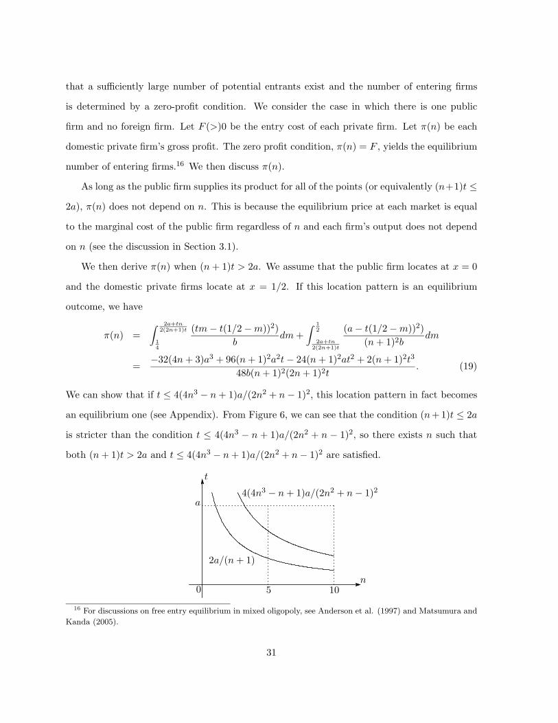
We can show that if t ≤ 4(4n3 − n + 1)a/(2n2 + n − 1)2, this location pattern in fact becomes
an equilibrium one (see Appendix). From Figure 6, we can see that the condition (n+1)t ≤ 2a
is stricter than the condition t ≤ 4(4n3 − n + 1)a/(2n2 + n − 1)2, so there exists n such that
both (n + 1)t > 2a and t ≤ 4(4n3 − n + 1)a/(2n2 + n − 1)2 are satisfied.
t
0n
105
a
2a/(n + 1)
4(4n3 − n + 1)a/(2n2 + n − 1)2
16 For discussions on free entry equilibrium in mixed oligopoly, see Anderson et al. (1997) and Matsumura and
Kanda (2005).
31
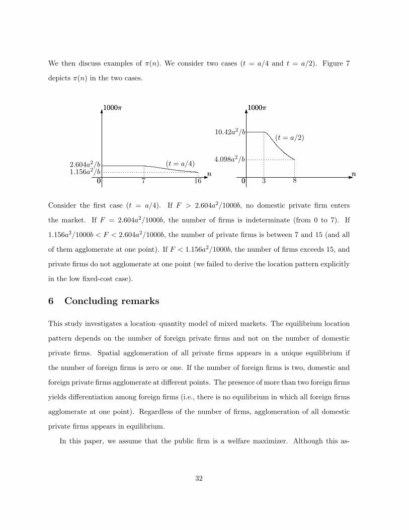
We then discuss examples of π(n). We consider two cases (t = a/4 and t = a/2). Figure 7
depicts π(n) in the two cases.
2.604a2/b
0n
16
1000π
(t = a/4)1.156a2/b
0n
7
1000π
0n
1000π
10.42a2/b
0n
1000π
(t = a/2)
4.098a2/b
3 8
Consider the first case (t = a/4). If F > 2.604a2/1000b, no domestic private firm enters
the market. If F = 2.604a2/1000b, the number of firms is indeterminate (from 0 to 7). If
1.156a2/1000b < F < 2.604a2/1000b, the number of private firms is between 7 and 15 (and all
of them agglomerate at one point). If F < 1.156a2/1000b, the number of firms exceeds 15, and
private firms do not agglomerate at one point (we failed to derive the location pattern explicitly
in the low fixed-cost case).
6 Concluding remarks
This study investigates a location–quantity model of mixed markets. The equilibrium location
pattern depends on the number of foreign private firms and not on the number of domestic
private firms. Spatial agglomeration of all private firms appears in a unique equilibrium if
the number of foreign firms is zero or one. If the number of foreign firms is two, domestic and
foreign private firms agglomerate at different points. The presence of more than two foreign firms
yields differentiation among foreign firms (i.e., there is no equilibrium in which all foreign firms
agglomerate at one point). Regardless of the number of firms, agglomeration of all domestic
private firms appears in equilibrium.
In this paper, we assume that the public firm is a welfare maximizer. Although this as-
32

sumption is very popular among the models of mixed oligopoly,17 other approaches also exist.18
Deviation from this welfare-maximizing assumption and the application of other approaches to
this problem remain topics for future research.
[2005.07.11 711]
17 See, among others, Anderson, de Palma, and Thisse (1997), De Fraja and Delbono (1989), Fjell and Pal
(1996), Pal (1998b), and Matsumura (1998).
18 See, e.g., Fershtman (1990) and Futagami (1999).
33
APPENDIX
Proof of Lemma 1 From (3), we obtain that b(q0 +∑
i∈D qi) = a − td(x, x0). This yields
Lemma 1(i). From (3), we obtain that
td(x, x0) = a − b
(q0 +
∑i∈D
qi
)≥ p(x) ≡ a − b
(q0 +
∑i∈D∪F
qi
). (20)
Thus, if d(x, x0) ≤ d(x, xi), p(x) ≤ td(x, x0) ≤ td(x, xi). That is, firm i’s cost is never lower
than the price, so it does not supply for the market, x. This yields Lemma 1(ii). Q.E.D.
Proof of Proposition 1 Proposition 1 obviously holds true if n = 1. Suppose that n ≥ 2.
We assume that there is no equilibrium where x1 = x2 and derive a contradiction. Suppose
that firm 2 deviates from the equilibrium strategy and chooses the same location as firm 1.
From Lemma 1, we have that the locations of all other firms are still optimal. Because of the
symmetries between all domestic private firms this location is best for firm 2 since it is best for
firm 1. Thus, this location pattern constitutes an equilibrium, a contradiction. Q.E.D.
Proof of Proposition 2 We have already shown that the location of private firms does not
affects the profits of each private firm. Thus, if Proposition 2 holds true when n = 1, it also
holds true for any n ≥ 1. Thus, we prove Proposition 2 in the case of n = m = 1. Suppose that
firm 1 (firm 2) is a domestic (foreign) private firm.
First, we show that the optimal location of firm 2 is 1/2 given that x0 = 0 and x1 = 1/2.
By symmetry, without loss of generality, we assume that x2 ∈ [0, 1/2]. Since no other foreign
firm exists, q2(x) in (7) is positive if and only if td(x, x0) > td(x, x2). Therefore, firm 2 supplies
at x ∈ (x2/2, (1 + x2)/2). For x ∈ (x2/2, (1 + x2)/2), the quantity supplied by firm 2 is
q2(x) =td(x, x0) − td(x, x2)
2b. (21)
From (8), firm 2’s profit is:
π2 =∫ x2
x22
(tx + t(x2 − x) − 2t(x2 − x))2
4bdx +
∫ 12
x2
(tx + t(x − x2) − 2t(x − x2))2
4bdx
+∫ 1+x2
2
12
(t(1 − x) + t(x − x2) − 2t(x − x2))2
4bdx =
t2x22(3 − 4x2)
24b. (22)
34

Differentiating π2 with respect to x2, we have ∂π2/∂x2 = (t2x2(1 − 2x2))/4b ≥ 0. This implies
that the best reply of firm 2 is x2 = 1/2.
Next, we show that firm 1’s best location is x1 = 1/2 given the others’ locations. By
symmetry, without loss of generality, we assume that x1 ∈ [0, 1/2]. We consider the following
two segments: (1) x1 ∈ [0, 1/4] and (2) x1 ∈ (1/4, 1/2].
(1) x1 ∈ [0, 1/4]: From Lemma 1(ii), firm 1 does not supply at x ∈ [0, x1/2], so its profit
from market x ∈ [0, x1/2] is zero. From Lemma 1(ii), firm 2 does not supply at x ∈ [0, 1/4].
From (8), firm 1’s profit at x ∈ (x1/2, 1/4] is
π1(x) =(tx − td(x1, x))2
b. (23)
Consider the market x > 1/4. From Lemma 1(ii), firm 1 does not supply for the market
x ≥ 3/4(≥ (x1 + 1)/2). In the former part of this proof, we have already shown that firm 2
supplies at x ∈ (1/4, 3/4) (since x2 = 1/2). From (7) and (21), firm 1 supplies only for the
market x < (1 + 4x1)/4. For the market x ∈ (1/4, (1 + 4x1)/4), the profit of firm 1 is given by
π1(x) =(tx + td(x2, x) − 2td(x1, x))2
4b. (24)
Thus, the total profit of the domestic firm is:
π1 =∫ x1
x12
(tx − t(x1 − x))2
bdx +
∫ 14
x1
(tx − t(x − x1))2
bdx
+∫ 1+4x1
4
14
(tx + t(12 − x) − 2t(x − x1))2
4bdx =
t2x21(1 − 2x1)
4b. (25)
Differentiating π1 with respect to x1, we have:
∂π1
∂x1=
t2x1(1 − 3x1)2b
> 0. (26)
(2) x1 ∈ (1/4, 1/2]: From Lemma 1(ii), firm 1 does not supply at x ∈ [0, x1/2], so its profit
from market x ∈ [0, x1/2] is zero. From Lemma 1(ii), firm 2 does not supply at x ∈ [0, 1/4].
From (8), firm 1’s profit at x ∈ (x1/2, 1/4] is given by (23).
Consider the market x > 1/4. From Lemma 1(ii) firm 1 does not supply for the market
x ≥ 3/4(≥ (x1 + 1)/2). In the former part of this proof, we have already shown that firm 2
35

supplies at x ∈ (1/4, 3/4) (since x2 = 1/2). From (7) and (21), firm 1 supplies only for the
market x < (1 + 4x1)/4. For the market x ∈ (1/4, (1 + 4x1)/4), the profit of firm 1 is given by
(24). Noting that (1 + 4x1)/4 ≥ 1/2, we have that the resulting profit of firm 1 is:
π1 =∫ 1
4
x12
(tx − t(x1 − x))2
bdx +
∫ x1
14
(tx + t(1/2 − x) − 2t(x1 − x))2
4bdx
+∫ 1
2
x1
(tx + t(1/2 − x) − 2t(x − x1))2
4bdx +
∫ 1+4x14
12
(t(1 − x) + t(x − 1/2) − 2t(x − x1))2
4bdx
=t2(16x3
1 − 24x21 + 12x1 − 1)
96b. (27)
Differentiating π1 with respect to x1, we have:
∂π1
∂x1=
t2(1 − 2x1)2
8b≥ 0. (28)
(26) and (28) imply that the optimal location of firm 1 is x1 = 1/2. Q.E.D.
Proof of Proposition 3 For the same reason in Proof of Proposition 2, we consider the case
in which n = 1 and m = 2. Suppose that firm 1 is domestic and firms 2 and 3 are foreign.
Proof of Proposition 3(i) First, we show that the location pattern, x2 = x3 = 1/2, is
an equilibrium outcome. By symmetry, without loss of generality, we assume that the best
response of firm 2 is x2 = 1/2 given that x0 = 0 and x3 = 1/2. We consider 3 segments: (1)
x2 ∈ [0, 1/4], (2) x2 ∈ (1/4, 1/3], and (3) x2 ∈ (1/3, 1/2].
(1) x2 ∈ [0, 1/4] From Lemma 1(ii) and (7), on [0, 1/4], firm 3 does not supply but firm 2
supplies at x ∈ [x2/2, 1/4]. On [1/4, (x2 + 1/2)/2], the quantity supplied by firm 2 is positive.
On this range the quantity supplied by firm 3 is
q3(x) = max{
td(x, x0) + td(x, x2) − 2td(x, x3)3b
, 0}
= max{
tx + t(x − x2) − 2t(1/2 − x)3b
, 0}
.(29)
For any x ∈ ((1+x2)/4, (x2 +1/2)/2], tx+ t(x−x2)− 2t(1/2−x) is positive, and it is negative
for x ≤ (1 + x2)/4. This implies that firm 3 also supplies for x ∈ ((1 + x2)/4, (x2 + 1/2)/2] but
does not supply for x ≤ (1 + x2)/4. On ((x2 + 1/2)/2, 1/2], the quantity supplied by firm 3 is
positive, and that supplied by firm 2 is
q2(x) = max{
td(x, x0) + td(x, x3) − 2td(x, x2)3b
, 0}
= max{
tx + t(1/2 − x) − 2t(x − x2)3b
, 0}
.(30)
36
For any x ∈ [(x2+1/2)/2, (1+4x2)/4), tx+t(1/2−x)−2t(x−x2) is positive, and it is non-positive
for x ∈ [(1 + 4x2)/4, 1/2]. This implies that firm 2 supplies for x ∈ [(x2 + 1/2)/2, (1 + 4x2)/4)
but not for x ∈ [(1 + 4x2)/4, 1/2]. From Lemma 1(ii) firm 2 does not supply for x ∈ [1/2, 1].
We summarize the discussion as follows: (a) firm 2 does not supply at x ∈ [0, x2/2] and
x ∈ [(1 + 4x2)/4, 1]; (b) firm 2 and firm 0 supply at x ∈ [x2/2, (1 + x2)/4]; (c) firm 2, firm 3,
and firm 0 supply at x ∈ [(1 + x2)/4, (1 + 4x2)/4]. The resulting profit of firm 2 is:
π2 =∫ x2
x22
(tx − t(x2 − x))2
4bdx +
∫ 1+x24
x2
(tx − t(x − x2))2
4bdx
+∫ 1+4x2
4
1+x24
(tx + t(1/2 − x) − 2t(x − x2))2
9bdx
=t2x2
2(3 − 4x2)48b
. (31)
For any x2 ∈ [0, 1/4], π2 is non-decreasing, and it is increasing for x2 ∈ (0, 1/4].
(2) x2 ∈ (1/4, 1/3] From the same discussions in segment (1), we obtain the following
supply pattern, which is exactly the same as that in segment (1). (a) firm 2 does not supply at
x ∈ [0, x2/2] and x ∈ [(1 + 4x2)/4, 1]; (b) firm 2 and firm 0 supply at x ∈ [x2/2, (1 + x2)/4]; (c)
firm 2, firm 3, and firm 0 supply at x ∈ [(1 + x2)/4, (1 + 4x2)/4]. The profit of firm 2 is:
π2 =∫ x2
x22
(tx − t(x2 − x))2
4bdx +
∫ 1+x24
x2
(tx − t(x − x2))2
4bdx
+∫ 1
2
1+x24
(tx + t(12 − x) − 2t(x − x2))2
9bdx +
∫ 1+4x24
12
(t(1 − x) + t(x − 12) − 2t(x − x2))2
9bdx
=t2x2
2(3 − 4x2)48b
. (32)
For any x2 ∈ (1/4, 1/3], π2 is increasing.
(3) x2 ∈ (1/3, 1/2] The range for which firm 2 supplies is exactly the same as that in
segments (1) and (2). We focus the different points only. On [1/4, x2], the quantity supplied by
firm 3 is
q3(x) = max{ td(x, x0) + td(x, x2) − 2td(x, x3)
3b, 0}
= max{ tx + t(x2 − x) − 2t(1/2 − x)
3b, 0}.(33)
For this range, tx + t(x2 − x)− 2t(1/2− x) > 0, if and only if x ∈ ((1− x2)/2, x2]. Thus, q3(x)
37
is positive if and only if x ∈ ((1−x2)/2, x2]. Note that threshold value is (1−x2)/2 in segment
(3), while it is (1 + x2)/4 in segments (1) and (2).
The following is the supply pattern in this case. (a) firm 2 does not supply at x ∈ [0, x2/2]
and x ∈ [(1 + 4x2)/4, 1]; (b) firm 2 and firm 0 supply at x ∈ [x2/2, (1 − x2)/2]; (c) firm 2, firm
3, and firm 0 supply at x ∈ ((1 − x2)/2, (1 + 4x2)/4). Thus, the profit of firm 2 is:
π2 =∫ 1−x2
2
x22
(tx − t(x2 − x))2
4b+∫ x2
1−x22
(tx + t(1/2 − x) − 2t(x2 − x))2
9bdx
+∫ 1
2
x2
(tx + t(1/2 − x) − 2t(x − x2))2
9bdx
+∫ 1+4x2
4
12
(t(1 − x) + t(x − 1/2) − 2t(x − x2))2
9bdx
=t2(−7 + 54x2 − 108x2
2 + 72x32)
432b. (34)
Differentiating it, we have ∂π2/∂x2 = (t2(1 − 2x2)2)/8b ≥ 0. Since π2 is non-decreasing in
x2 ∈ [0, 1/2] and increasing in x2 ∈ (0, 1/2), we have that π2 is maximized at x2 = 1/2. The
profit is
π2 =t2
216b. (35)
Next, we show that, given the above locations of firms 2 and 3 (the foreign firms), firm
1’s (the domestic firm’s) best reply is x1 = 5−√3
11 . By symmetry, without loss of generality,
we assume that x1 ∈ [0, 1/2]. We consider the following 2 segments: (1) x1 ∈ [0, 1/3] and (2)
x1 ∈ (1/3, 1/2].
(1) x1 ∈ [0, 1/3] From the former part of the proof, we have that the quantity of each foreign
firm is positive if and only if x ∈ (1/4, 3/4). Firm 1 supplies for the market x ∈ (x1/2, 1/4], and
it is given by
q1(x) =(tx − td(x1, x))
b. (36)
Consider the market x ∈ (1/4, 1/2]. As is shown in the former part of this proof, the quantity
supplied by firm 2 (and that by firm 3) is
q2(x) =td(x, x0) + td(x, x3) − 2td(x, x2)
3b=
tx − t(1/2 − x)3b
. (37)
38
From (7), on (1/4, 1/2], the quantity supplied by firm 1 is
q1(x) = max{ tx + 2t(1/2 − x) − 3t(x − x1)
3b, 0}. (38)
tx + 2t(1/2 − x) − 3t(x − x1) is positive if and only if x ∈ (1/4, (1 + 3x1)/4). Thus, firm 1
supplies for the market x if and only if x ∈ (1/4, (1 + 3x1)/4). From a similar discussion, we
have that firm 1 does not supply for the market x ∈ [(1 + 3x1)/4, 1].
We summarize the discussion as follows: (a) firm 1 does not supply at x ∈ [0, x1/2] and
x ∈ [(1 + 3x1)/4, 1]; (b) firm 1 and firm 0 supply at x ∈ [x1/2, 1/4]; (c) firm 1, firm 2, firm 3,
and firm 0 supply at x ∈ [1/4, (1 + 3x1)/4]. The profit of firm 1 is:
π1 =∫ 1
4
x12
(tx − t(x1 − x))2
bdx +
∫ x1
14
(tx + 2t(1/2 − x) − 3t(x1 − x))2
9bdx
+∫ 1+3x1
4
x1
(tx + 2t(1/2 − x) − 3t(x − x1))2
9b
=t2(22x3
1 − 30x21 + 12x1 − 1)
72b. (39)
The first-order condition of optimality is:
∂π1
∂x1= 0 ⇔ t2(2 − 10x1 + 11x2
1)12b
= 0. (40)
This yields
x1 =5 −√
311
. (41)
(2) x1 ∈ (1/3, 1/2] From the former part of the proof, we have that the quantity of
each foreign firm is positive if and only if x ∈ (1/4, 3/4). Firm 1 supplies for the market
x ∈ (x1/2, 1/4], and it is given by (36). Consider the market x ∈ (1/4, 1/2]. The quantity
supplied by firm 2 (and that by firm 3) is given by (37). From (7), on (1/4, 1/2], the quantity
supplied by firm 1 is
q1(x) = max{ tx + 2t(1/2 − x) − 3t(x − x1)
3b, 0}. (42)
tx + 2t(1/2 − x) − 3t(x − x1) is positive for all x ∈ (1/4, 1/2] because x1 > 1/3. Thus, firm 1
supplies for these markets. On [1/2, 3/4], the quantity supplied by firm 1 is
q1(x) = max{ t(1 − x) + 2t(x − 1/2) − 3t(x − x1)
3b, 0}. (43)
39
t(1−x)+2t(x−1/2)−3t(x−x1) is positive if and only if x ∈ (1/2, 3x1/2). Thus, on this range
(x ∈ (1/2, 3/4]), firm 1 supplies for the market x if and only if x ∈ (1/2, 3x1/2). On [3/4, 1],
firm 1 does not supply (Lemma 1(ii)).
We summarize the discussion as follows: (a) firm 1 does not supply at x ∈ [0, x1/2] and
x ∈ [3x1/2, 1]; (b) firm 1 and firm 0 supply at x ∈ (x1/2, 1/4]; (c) firm 1, firm 2, firm 3, and
firm 0 supply at x ∈ (1/4, 3x1/2]. The profit of firm 1 is:
π1 =∫ 1
4
x12
(tx − t(x1 − x))2
bdx +
∫ x1
14
(tx + 2t(1/2 − x) − 3t(x1 − x))2
9bdx
+∫ 1
2
x1
(tx + 2t(1/2 − x) − 3t(x − x1))2
9bdx
+∫ 3x1
2
12
(t(1 − x) + 2t(x − 1/2) − 3t(x − x1))2
9bdx
=t2(120x3
1 − 144x21 + 54x1 − 5)
216b. (44)
Differentiating π1 with respect to x1, we have:
∂π1
∂x1=
t2(1 − 2x1)(3 − 10x1)12b
< 0. (45)
This implies that no x ∈ (1/3, 1/2] maximizes π1. Q.E.D.
Proof of Proposition 3(ii) First, we show that the location pattern, x2 = 13/30 and
x3 = 17/30 constitutes an equilibrium. By symmetry, it is sufficient to show that the best
response of firm 2 is x2 = 13/30 given that x0 = 0 and x3 = 17/30. To show the best
response, we consider the following 8 segments: (1) x2 ∈ [0, 13/60], (2) x2 ∈ (13/60, 7/20], (3)
x2 ∈ (7/20, 17/45], (4) x2 ∈ (17/45, 1/2], (5) x2 ∈ (1/2, 17/30], (6) x2 ∈ (17/30, 32/45], (7)
x2 ∈ (32/45, 47/60], and (8) x2 ∈ (47/60, 1].
(1) x2 ∈ [0, 13/60]
π2 =∫ x2
x22
(tx − t(x2 − x))2
4bdx +
∫ 17+15x260
x2
(tx − t(x − x2))2
4bdx
+∫ 17+60x2
60
17+15x260
(tx + t(17/30 − x) − 2t(x − x2))2
9bdx
=t2x2
2(17 − 20x2)240b
. (46)
40

For any x2 ∈ [0, 13/60], π2 is non-decreasing and it is increasing for x2 ∈ (0, 13/60].
(2) x2 ∈ (13/60, 7/20]
π2 =∫ x2
x22
(tx − t(x2 − x))2
4bdx +
∫ 17+15x260
x2
(tx − t(x − x2))2
4bdx
+∫ 1
2
17+15x260
(tx + t(17/30 − x) − 2t(x − x2))2
9bdx
+∫ 47+60x2
120
12
(t(1 − x) + t(17/30 − x) − 2t(x − x2))2
9bdx
=t2(2197 − 30420x2 + 346950x2
2 − 459000x32)
2916000b. (47)
For any x2 ∈ (13/60, 7/20], π2 is increasing.
(3) x2 ∈ (7/20, 17/45]
π2 =∫ x2
x22
(tx − t(x2 − x))2
4bdx +
∫ 17+15x260
x2
(tx − t(x − x2))2
4bdx
+∫ 1
2
17+15x260
(tx + t(17/30 − x) − 2t(x − x2))2
9bdx
+∫ 17
30
12
(t(1 − x) + t(17/30 − x) − 2t(x − x2))2
9bdx
+∫ 13+60x2
60
1730
(t(1 − x) + t(x − 17/30) − 2t(x − x2))2
9bdx
=t2(−3532 + 24480x2 + 60075x2
2 − 121500x32)
1458000b. (48)
For any x2 ∈ (7/20, 17/45], π2 is increasing.
(4) x2 ∈ (17/45, 1/2]
π2 =∫ 17−15x2
30
x22
(tx − t(x2 − x))2
4bdx +
∫ x2
17−15x230
(tx + t(1730 − x) − 2t(x2 − x))2
9bdx
+∫ 1
2
x2
(tx + t(1730 − x) − 2t(x − x2))2
9bdx
+∫ 17
30
12
(t(1 − x) + t(1730 − x) − 2t(x − x2))2
9bdx
+∫ 13+60x2
60
1730
(t(1 − x) + t(x − 1730) − 2t(x − x2))2
9bdx
=t2(−12641 + 86190x2 − 152100x2
2 + 81000x32)
486000b. (49)
41

The first-order condition for the optimality is:
∂π2
∂x2= 0 ⇐⇒ t2(13 − 30x2)(221 − 270x2)
16200b= 0. (50)
The second-order condition is satisfied. From this condition, we find that π2 is maximized at
x2 = 13/30. The profit is
π2 =1369t2
243000b. (51)
(5) x2 ∈ (1/2, 17/30]
π2 =∫ 17−15x2
30
x22
(tx − t(x2 − x))2
4bdx +
∫ 12
17−15x230
(tx + t(1730 − x) − 2t(x2 − x))2
9bdx
+∫ x2
12
(t(1 − x) + t(1730 − x) − 2t(x2 − x))2
9bdx
+∫ 17
30
x2
(t(1 − x) + t(1730 − x) − 2t(x − x2))2
9bdx
+∫ 13+60x2
60
1730
(t(1 − x) + t(x − 1730) − 2t(x − x2))2
9bdx
=t2(−30641 + 194190x2 − 368100x2
2 + 225000x32)
486000b. (52)
For any x2 ∈ (1/2, 17/30], π2 is decreasing.
(6) x2 ∈ (17/30, 32/45]
π2 =∫ 1
2
−17+60x260
(tx + t(17/30 − x) − 2t(x2 − x))2
9bdx
+∫ 17
30
12
(t(1 − x) + t(17/30 − x) − 2t(x2 − x))2
9bdx
+∫ x2
1730
(t(1 − x) + t(x − 17/30) − 2t(x2 − x))2
9bdx
+∫ 32−15x2
30
x2
(t(1 − x) + t(x − 17/30) − 2t(x − x2))2
9bdx
+∫ 1+x2
2
32−15x230
(t(1 − x) − t(x − x2))2
4bdx
=t2(75119 − 301770x2 + 456300x2
2 − 243000x32)
1458000b. (53)
For any x2 ∈ (17/30, 32/45], π2 is decreasing.
42

(7) x2 ∈ (32/45, 47/60]
π2 =∫ 1
2
−17+60x260
(tx + t(17/30 − x) − 2t(x2 − x))2
9bdx
+∫ 17
30
12
(t(1 − x) + t(17/30 − x) − 2t(x2 − x))2
9bdx
+∫ 32+15x2
60
1730
(t(1 − x) + t(x − 17/30) − 2t(x2 − x))2
9bdx
+∫ x2
32+15x260
(t(1 − x) − t(x2 − x))2
4bdx
+∫ 1+x2
2
x2
(t(1 − x) − t(x − x2))2
4bdx
=t2(−5339 + 46290x2 − 80775x2
2 + 40500x32)
486000b. (54)
For any x2 ∈ (32/45, 47/60], π2 is decreasing.
(8) x2 ∈ (47/60, 1]
π2 =∫ 32+15x2
60
x2− 1360
(t(1 − x) + t(x − 17/30) − 2t(x2 − x))2
9bdx
+∫ x2
32+15x260
(t(1 − x) − t(x2 − x))2
4bdx +
∫ 1+x22
x2
(t(1 − x) − t(x − x2))2
4bdx
=t2(1 − x2)2(20x2 − 7)
240b. (55)
For any x2 ∈ (47/60, 1], π2 is non-increasing.
Next, we derive the location pattern in which the foreign firms locate at x2 = 13/30 and
x3 = 17/30. By symmetry, without loss of generality, we assume that x1 ∈ [0, 1/2]. To show
the best response, we have to consider 8 segments: (1) x1 ∈ [0, 2/15], (2) x1 ∈ (2/15, 13/60],
(3) x1 ∈ (13/60, 11/45], (4) x1 ∈ (11/45, 13/45], (5) x1 ∈ (13/45, 7/20], (6) x1 ∈ (7/20, 17/45],
(7) x1 ∈ (17/45, 13/30], and (8) x1 ∈ (13/30, 1/2].
(1) x1 ∈ [0, 2/15]
π1 =∫ x1
x12
(tx − t(x1 − x))2
bdx +
∫ 1360
x1
(tx − t(x − x1))2
bdx
+∫ 13+60x1
60
1360
(tx + t(13/30 − x) − 2t(x − x1))2
4bdx
43

=t2x2
1(13 − 30x1)60b
. (56)
For any x1 ∈ [0, 2/15], π1 is non-decreasing.
(2) x1 ∈ (2/15, 13/60]
π1 =∫ x1
x12
(tx − t(x1 − x))2
bdx +
∫ 1360
x1
(tx − t(x − x1))2
bdx
+∫ 7
20
1360
(tx + t(13/30 − x) − 2t(x − x1))2
4bdx
+∫ 1+3x1
4
720
(tx + t(13/30 − x) + t(17/30 − x) − 3t(x − x1))2
9bdx
=t2(−23625x3
1 + 10125x21 − 180x1 + 8)
40500b. (57)
For any x1 ∈ (2/15, 13/60], π1 is increasing.
(3) x1 ∈ (13/60, 11/45]
π1 =∫ 13
60
x12
(tx − t(x1 − x))2
bdx +
∫ x1
1360
(tx + t(13/30 − x) − 2t(x1 − x))2
4bdx
+∫ 7
20
x1
(tx + t(13/30 − x) − 2t(x − x1))2
4bdx
+∫ 1+3x1
4
720
(tx + t(13/30 − x) + t(17/30 − x) − 3t(x − x1))2
9bdx
=t2(3000x3
1 − 6600x21 + 3220x1 − 237)
36000b. (58)
For any x1 ∈ (13/60, 11/45], π1 is increasing.
(4) x1 ∈ (11/45, 13/45]
π1 =∫ 13
60
x12
(tx − t(x1 − x))2
bdx +
∫ x1
1360
(tx + t(13/30 − x) − 2t(x1 − x))2
4bdx
+∫ 7
20
x1
(tx + t(13/30 − x) − 2t(x − x1))2
4bdx
+∫ 13
30
720
(tx + t(13/30 − x) + t(17/30 − x) − 3t(x − x1))2
9bdx
+∫ 2+45x1
30
1330
(tx + t(x − 13/30) + t(17/30 − x) − 3t(x − x1))2
9bdx
=t2(194400x3
1 − 213840x21 + 78300x1 − 5969)
583200b. (59)
44
For any x1 ∈ (11/45, 13/45], π1 is increasing.
(5) x1 ∈ (13/45, 7/20]
π1 =∫ 13
60
x12
(tx − t(x1 − x))2
bdx +
∫ x1
1360
(tx + t(13/30 − x) − 2t(x1 − x))2
4bdx
+∫ 7
20
x1
(tx + t(13/30 − x) − 2t(x − x1))2
4bdx
+∫ 13
30
720
(tx + t(13/30 − x) + t(17/30 − x) − 3t(x − x1))2
9bdx
+∫ 1
2
1330
(tx + t(x − 13/30) + t(17/30 − x) − 3t(x − x1))2
9bdx
+∫ 17+45x1
60
12
(t(1 − x) + t(x − 13/30) + t(17/30 − x) − 3t(x − x1))2
9bdx
=t2(243000x3
1 − 437400x21 + 208980x1 − 12269)
2916000b. (60)
Differentiating π1 with respect to x1, we have:
∂π1
∂x1=
t2(150x21 − 180x1 + 43)
600b. (61)
From the first-order condition of the optimality, we have
x1 =18 −√
6630
∼ 0.329. (62)
(6) x1 ∈ (7/20, 17/45]
π1 =∫ 13
60
x12
(tx − t(x1 − x))2
bdx +
∫ 720
1360
(tx + t(13/30 − x) − 2t(x1 − x))2
4bdx
+∫ x1
720
(tx + t(13/30 − x) + t(17/30 − x) − 3t(x1 − x))2
9bdx
+∫ 13
30
x1
(tx + t(13/30 − x) + t(17/30 − x) − 3t(x − x1))2
9bdx
+∫ 1
2
1330
(tx + t(x − 13/30) + t(17/30 − x) − 3t(x − x1))2
9bdx
+∫ 17+45x1
60
12
(t(1 − x) + t(x − 13/30) + t(17/30 − x) − 3t(x − x1))2
9bdx
=t2(222750x3
1 − 279450x21 + 111780x1 − 10013)
729000b. (63)
45
For any x1 ∈ (7/20, 17/45], π1 is decreasing.
(7) x1 ∈ (17/45, 13/30]
π1 =∫ 13
60
x12
(tx − t(x1 − x))2
bdx +
∫ 720
1360
(tx + t(13/30 − x) − 2t(x1 − x))2
4bdx
+∫ x1
720
(tx + t(13/30 − x) + t(17/30 − x) − 3t(x1 − x))2
9bdx
+∫ 13
30
x1
(tx + t(13/30 − x) + t(17/30 − x) − 3t(x − x1))2
9bdx
+∫ 1
2
1330
(tx + t(x − 13/30) + t(17/30 − x) − 3t(x − x1))2
9bdx
+∫ 17
30
12
(t(1 − x) + t(x − 13/30) + t(17/30 − x) − 3t(x − x1))2
9bdx
+∫ 3x1
2
1730
(t(1 − x) + t(x − 13/30) + t(x − 17/30) − 3t(x − x1))2
9bdx
=t2(135000x3
1 − 162000x21 + 63270x1 − 6613)
243000b. (64)
For any x1 ∈ (17/45, 13/30], π1 is decreasing.
(8) x1 ∈ (13/30, 1/2]
π1 =∫ 7
20
−13+60x160
(tx + t(13/30 − x) − 2t(x1 − x))2
4bdx
+∫ 13
30
720
(tx + t(13/30 − x) + t(17/30 − x) − 3t(x1 − x))2
9bdx
+∫ x1
1330
(tx + t(x − 13/30) + t(17/30 − x) − 3t(x1 − x))2
9bdx
+∫ 1
2
x1
(tx + t(x − 13/30) + t(17/30 − x) − 3t(x − x1))2
9bdx
+∫ 17
30
12
(t(1 − x) + t(x − 13/30) + t(17/30 − x) − 3t(x − x1))2
9bdx
+∫ 13
20
1730
(t(1 − x) + t(x − 13/30) + t(x − 17/30) − 3t(x − x1))2
9bdx
+∫ 13+60x1
60
1320
(t(1 − x) + t(x − 17/30) − 2t(x − x1))2
4bdx
=t2(487 − 2400x1 + 4650x2
1 − 3000x31)
13500b. (65)
For any x1 ∈ (13/30, 1/2], π1 is decreasing. Q.E.D.
46
Proof of Proposition 4 We assume that all foreign firms agglomerate at h in an equilibrium
and derive a contradiction. Without loss of generality, we assume that h ≤ 1/2.
First, we assume that h < 1/2 and show that, a foreign firm can enhance its profit if it
deviates from the equilibrium strategy and relocates at h + ε, where ε is small and positive
constant. The profit of each foreign firm in the equilibrium is:
π =∫ h
h2
[tx + mt(h − x) − (m + 1)t(h − x)]2
(m + 1)2bdx
+∫ 1
2
h
[tx + mt(x − h) − (m + 1)t(x − h)]2
(m + 1)2bdx
+∫ 1+h
2
12
[t(1 − x) + mt(x − h) − (m + 1)t(x − h)]2
(m + 1)2bdx
=h2(3 − 4h)t2
6b(m + 1)2. (66)
When a foreign firm relocates from h to h + ε, the firm’s profit becomes:
π =∫ h
h+mε2
[tx + (m − 1)t(h − x) + t(h + ε − x) − (m + 1)t(h + ε − x)]2
(m + 1)2bdx
+∫ h+ε
h
[tx + (m − 1)t(x − h) + t(h + ε − x) − (m + 1)t(h + ε − x)]2
(m + 1)2bdx
+∫ 1
2
h+ε
[tx + (m − 1)t(x − h) + t(x − h − ε) − (m + 1)t(x − h − ε)]2
(m + 1)2bdx
+∫ 1+h−ε
2
12
[t(1 − x) + (m − 1)t(x − h) + t(x − h − ε) − (m + 1)t(x − h − ε)]2
(m + 1)2bdx
+∫ 1+h+ε
2
1+h−ε2
[t(1 − x) − t(x − h − ε)]2
4bdx
=[h2(3 − 4h) + 6(1 − 2h)hmε + 3(m − 4h)mε2 + (1 + m − 5m2 − m3)ε3]t2
6b(m + 1)2. (67)
The difference between π in (67) and π in (66) is:
[6(1 − 2h)hm + 3(m − 4h)mε + (1 + m − 5m2 − m3)ε2]εt2
6b(m + 1)2. (68)
For any h < 1/2 and sufficiently small ε, this is positive, a contradiction.
Next, we assume that h = 1/2. We show that a foreign firm is able to enhance its profit if
it relocates from 1/2 to y < 1/2, where y is sufficiently close to 1/2.
47
From (66), the profit of each foreign firm in the equilibrium is
π =t2
24b(m + 1)2. (69)
If a foreign firm relocates at y < 1/2, the profit of the firm is:
π =∫ 1−y
2
y2
(tx − t(y − x))2
4bdx +
∫ y
1−y2
[tx + (m − 1)t(12 − x) + t(h − x) − (m + 1)t(y − x)]2
(m + 1)2bdx
+∫ 1
2
y
[tx + (m − 1)t(12 − x) + t(x − y) − (m + 1)t(x − y)]2
(m + 1)2bdx
+∫ 3−m+2ym
4
12
[t(1 − x) + (m − 1)t(x − 12) + t(h − y) − (m + 1)t(x − y)]2
(m + 1)2bdx
=[8(m3 + 5m2 − 9m − 1)y3 − 12(m3 + 3m2 − 5m − 1)y2]t2
48b(m + 1)2
+[6(m − 1)(m + 1)2y − (m − 1)(m2 + 3)]t2
48b(m + 1)2. (70)
The difference between π in (70) and π in (69) is:
(1 − 2y)2(1 − 3m + m2 − m3 − 2(1 + 9m − 5m2 − m3)y)t2
48b(m + 1)2. (71)
For any y which is close to 1/2, this is positive since limy→1/2 (1− 3m + m2 −m3 − 2(1 + 9m−5m2 − m3)y) = 6m(m − 2) > 0, a contradiction. Q.E.D.
Proof of the result in Section 5.3 Suppose that there are one public firm, n domestic
private firms and no foreign firm. Without loss of generality, we assume that x0 = 0. We then
prove that the domestic private firms locate at x = 1/2 in equilibrium if t ≤ 4(4n3 − n +
1)a/(2n2 + n − 1)2. We show that, given the locations of the public firm and the other private
firms, each private firm cannot increase its profit by relocating from the point 1/2.
We first consider the conditions that the public firm does not supply to a range on the
circular city. We consider three ranges: (i) m ∈ [0, x] (x is the location of the relocating firm),
(ii) m ∈ [x, 1/2], (iii) m ∈ [1/2, 1].
When the public firm does not supply at m ∈ [0, x], the following equation holds:
(n − 1)tm − t(1/2 − m)
b+
tm − t(x − m)b
>a − tm
b, m >
2a + (n − 1)t + 2tx
2(2n + 1)t≡ m1. (72)
48

m1 ≤ x, if and only if
2a + (n − 1)t4nt
< x ≤ 1/2. (73)
When the public firm does not supply at m ∈ [x, 1/2], the following equation holds:
(n − 1)tm − t(1/2 − m)
b+
tm − t(m − x)b
>a − tm
b, m >
2a + (n − 1)t − 2tx
2(2n − 1)t≡ m2. (74)
x ≤ m2 ≤ 1/2, if and only if
2a − nt
2t≤ x ≤ 2a + (n − 1)t
4nt. (75)
When the public firm does not supply at m ∈ [1/2, 1], the following equation holds:
(n − 1)t(1 − m) − t(m − 1/2)
b+
t(1 − m) − t(m − x)b
>a − t(1 − m)
b, (76)
m <−2a + (3n + 1)t + 2tx
2(2n + 1)t≡ m3. (77)
1/2 ≤ m3, if and only if
2a − nt
2t< x ≤ 1/2. (78)
From the discussions above, we can see that we have to consider following three cases:
(i) x ∈ [(2a + (n − 1)t)/4nt, 1/2] (the public firm does not supply at m ∈ [m1, m3]), (ii)
x ∈ [(2a − nt)/2t, (2a + (n − 1)t)/4nt] (the public firm does not supply at m ∈ [m2, m3]), (iii)
x ∈ [0, (2a − nt)/2t] (the public firm supplies at all points on the circular city).
(i) x ∈ [(2a+(n−1)t)/4nt, 1/2]. In the case, the public firm does not supply at m ∈ [m1, m3].
The profit of the private firm locating at x ∈ [(2a + (n − 1)t)/4nt, 1/2] is:
πi =∫ m1
x2
(tm − t(x − m))2
bdm +
∫ x
m1
(a + (n − 1)t(1/2 − m) − nt(x − m))2
(n + 1)2bdm
+∫ 1
2
x
(a + (n − 1)t(1/2 − m) − nt(m − x))2
(n + 1)2bdm
+∫ m3
12
(a + (n − 1)t(m − 1/2) − nt(m − x))2
(n + 1)2bdm +
∫ 1+x2
m3
(t(1 − m) − t(m − x))2
bdm
=8(n − 1)n(2n + 1)2t3x3
12b(n + 1)2(2n + 1)2t
49
+6t2(4(4n3 − n + 1)a + (4n4 − 4n3 − 3n2 − 1)t)x2 + 6(4n3 − n + 1)(4a − t)t2x
12b(n + 1)2(2n + 1)2t
+−8a3(4n + 3) + 24a2(n + 1)2t − 6a(4n3 + n2 + n + 2)t2 + (2n4 + 6n3 − n2 − n + 2)t3
12b(n + 1)2(2n + 1)2t.
Differentiating it with respect to x, we have:
∂πi
∂x=
t(1 − 2x)((4a − t)(4n3 − n + 1) + 2nt(1 + 3n − 4n3)x)2b(n + 1)2(2n + 1)2
. (79)
If t ≤ 4(4n3 − n + 1)a/(2n2 + n − 1)2, this is non-negative for any x ≤ 1/2.
(ii) x ∈ [(2a − nt)/2t, (2a + (n − 1)t)/4nt]. In this case, the public firm does not supply at
m ∈ [m2, m3]. The profit of the private firm locating at x ∈ [(2a − nt)/2t, (2a + (n − 1)t)/4nt]
is:
πi =∫ x
x2
(tm − t(x − m))2
bdm +
∫ m2
x
(tm − t(m − x))2
bdm
+∫ 1
2
m2
(a + (n − 1)t(1/2 − m) − nt(m − x))2
(n + 1)2bdm
+∫ m3
12
(a + (n − 1)t(m − 1/2) − nt(m − x))2
(n + 1)2bdm +
∫ 1+x2
m3
(t(1 − m) − t(m − x))2
bdm
= −8n(8n4 + 20n3 + 26n2 + 11n − 1)t3x3
12b(n + 1)2(2n + 1)2(2n − 1)t
+6(4(8n3 + 6n2 + n + 1)a + (8n5 + 4n4 + 2n3 − 3n2 − 6n − 1)t)t2x2
12b(n + 1)2(2n + 1)2(2n − 1)t
−6(4n3 − n + 1)(2a − nt)2tx + (6n2 + 3n − 1)(2a − nt)3
12b(n + 1)2(2n + 1)2(2n − 1)t.
Differentiating it with respect to x, we have:
h(x) ≡ −24n(8n4 + 20n3 + 26n2 + 11n − 1)t3x2
12b(n + 1)2(2n + 1)2(2n − 1)t
+12(4(8n3 + 6n2 + n + 1)a + (8n5 + 4n4 + 2n3 − 3n2 − 6n − 1)t)t2x
12b(n + 1)2(2n + 1)2(2n − 1)t
− 6(4n3 − n + 1)(2a − nt)2t12b(n + 1)2(2n + 1)2(2n − 1)t
.
We now show that h(x) is positive for any x ∈ [(2a−nt)/2t, (2a+(n− 1)t)/4nt]. We can easily
show that h′′(x) < 0. That is, h(x) is a concave function. On [(2a−nt)/2t, (2a+(n− 1)t)/4nt],
50
h(x) is minimized at one of the boundaries, x = (2a − nt)/2t or x = (2a + (n − 1)t)/4nt.
Substituting each of the boundaries into h(x), we have:
h
(2a − nt
2t
)=
(n + 1)2(2n − 1)(2n + 1)2(2a − nt)2((3 + 2n)t − 4a
24b(n + 1)2(2n + 1)2(2n − 1)t> 0,
h
(2a + (n − 1)t
4nt
)=
(2n − 1)48bn2(n + 1)2(2n + 1)2(2n − 1)t
×
[(n + 1)2(4n4 + 4n3 − n2 − n + 2)t3 − 3(n + 1)2(12n3 + 8n2 − 5n + 5)at2
+12(n + 1)(16n3 + 8n2 − 2n + 3)a2t − 4(52n3 + 24n2 − 3n + 7)a3].
We now define that k(t) ≡ (n + 1)2(4n4 + 4n3 − n2 − n + 2)t3 − 3(n + 1)2(12n3 + 8n2 − 5n +
5)at2+12(n+1)(16n3+8n2−2n+3)a2t−4(52n3+24n2−3n+7)a3. Substituting t = 2a/(n+1)
(the lowest value of t in this section) into k(t), we have
k
(2a
n + 1
)=
16n2(2n − 1)(2n + 1)2a3
(2n − 1)(n + 1)> 0. (80)
If k′(t) is positive for any t, k(t) is positive for any t > 2a/(n+1), that is, h((2a+(n−1)t)/4nt)
is positive. k′(t) is
k′(t) = 3(n + 1)2(4n4 + 4n3 − n2 − n + 2)t2
−6(n + 1)2(12n3 + 8n2 − 5n + 5)at + 12(n + 1)(16n3 + 8n2 − 2n + 3)a2.
This is a convex function and minimized at t = (12n3 +8n2−5n+5)a/(4n4 +4n3−n2−n+2).
Substituting it into k′(t), we have
k′(
(12n3 + 8n2 − 5n + 5)a4n4 + 4n3 − n2 − n + 2
)=
3(n − 1)(n + 1)(2n + 1)4(7n2 − 4n + 1)a2
4n4 + 4n3 − n2 − n + 2≥ 0.
We find that k′(t) is non negative and k(t) is non decreasing. k(t) is positive for any t >
2a/(n + 1), that is, h((2a + (n − 1)t)/4nt) is positive. Therefore, h(x) is positive for any
x ∈ [(2a−nt)/2t, (2a + (n− 1)t)/4nt], that is, the optimal location of the private firm does not
exist on [(2a − nt)/2t, (2a + (n − 1)t)/4nt].
(iii) x ∈ [0, (2a − nt)/2t]. In this case, the public firm supplies at all points on the circular
city. The profit of the private firm locating at x ∈ [0, (2a − nt)/2t] is:
πi =∫ x
x2
(tm − t(x − m))2
bdm +
∫ 12
x
(tm − t(m − x))2
bdm +
∫ 1+x2
12
(t(1 − m) − t(m − x))2
bdm
51

=t2x2(3 − 4x)
6b,
∂πi
∂x=
t2x(1 − 2x)b
.
πi is increasing with respect to x. This implies that the optimal location of the private firm
does not exist on [0, (2a − nt)/2t].
Accordingly, we have that the optimal location of the private firm is x = 1/2 if t ≤ 4(4n3 −n + 1)a/(2n2 + n − 1)2. Q.E.D.
52

References
Anderson, S. P., de Palma, A., Thisse, J.-F., 1997, Privatization and efficiency in a differenti-ated industry, European Economic Review 41, 1635–1654.
Anderson, S. P., Neven, D. J., 1991, Cournot competition yields spatial agglomeration, Inter-national Economic Review 32, 793–808.
Bos, D., 1986, Public Enterprise Economics (Amsterdam: North-Holland).
Bos, D., 1991, Privatization: A Theoretical Treatment (Oxford: Clarendon Press).
Chamorro-Rivas, J.-M., 2000, Plant proliferation in a spatial model of Cournot competition,Regional Science and Urban Economics 30, 507–518.
Corneo, G., Rob, R., 2003, Working in public and private firms, Journal of Public Economics87, 1335–1352.
Cremer, H., Marchand, M., Thisse, J.-F., 1991, Mixed oligopoly with differentiated products,International Journal of Industrial Organization 9, 43–53.
De Fraja, G., Delbono, F., 1989, Alternative strategies of a public enterprise in oligopoly,Oxford Economic Papers 41, 302–311.
Eaton, B. C., Schmitt, N., 1994, Flexible manufacturing and market structure, American Eco-nomic Review, 84, 875–888.
Fershtman, C., 1990, The interdependence between ownership status and market structure:the case of privatization, Economica 57, 319–328.
Fjell, K., Pal, D. 1996, A mixed oligopoly in the presence of foreign private firms, CanadianJournal of Economics 29, 737–743.
Futagami, K., 1999, The range of the public sector and efficiency, Financial Review 52, 1–13.
Gimeno, J., 1999, Reciprocal threats in multimarket rivalry: staking out spheres of influencein the U.S. airline industry, Strategic Management Journal 20, 101–28.
Greenhut, J. G., Greenhut, M. L., 1975, Spatial price discrimination, competition and loca-tional effects, Economica 42, 401–419.
Hamilton, J. H., Thisse, J.-F., Weskamp, A., 1989, Spatial discrimination: Bertrand vsCournot in a model of location choice, Regional Science and Urban Economics 19, 87–102.
Ide, I., Hayashi, T., 1992, Kinyu chiyukai ni okeru ko-teki bumon no yakuwari, in A. Horiuchiand N. Yoshino eds., Gendai Nihon no Kinyu Bunseki. (in Japanese)
Ishibashi, I, Matsumura, T., 2005, R&D Competition between public and private sectors,forthcoming in European Economic Review.
Matsumura, T., 1998, Partial privatization in mixed duopoly, Journal of Public Economics70, 473–483.
Matsumura, T., 2003a, Stackelberg mixed duopoly with a foreign competitor, Bulletin of Eco-nomic Research 55(3), 275–287.
53
Matsumura, T., 2003b, Consumer-benefiting exclusive territories, Canadian Journal of Eco-nomics 36(4), 1007–1025.
Matsumura, T., Matsushima, N. 2003, Mixed duopoly with product differentiation: sequentialchoice of location, Australian Economic Papers, 42, 18–34.
Matsumura, T., Kanda, O., 2005. Mixed oligopoly at free entry markets. Journal of Eco-nomics 84(1), 27–48.
Matsumura, T., Matsushima, N., 2004, Endogenous cost differentials between public and pri-vate enterprises: a mixed duopoly approach, Economica, 71, 671–688.
Matsushima, N., 2001, Horizontal mergers and merger waves in a location model, AustralianEconomic Papers 40, 263–286.
Matsushima, N., Matsumura, T. 2003, Mixed oligopoly and spatial agglomeration, CanadianJournal of Economics 36, 62–87.
Matsushima, N., Matsumura, T. 2005, Mixed oligopoly, foreign firms, and location choice,mimeo, available at http://norick.sakura.ne.jp/research/paper.html
Merrill, W., Schneider, N. 1966, Government firms in oligopoly industries: a short-run analy-sis, Quarterly Journal of Economics 80, 400–412.
Nett, L., 1993, Mixed oligopoly with homogeneous goods, Annals of Public and CooperativeEconomics 64, 367–393.
Nilssen, T., Sørgard, L. 2002, A public firm challenged by entry: duplication or diversity?Regional Science and Urban Economics 32, 259–274.
Norman, G., 1981, Spatial competition and spatial price discrimination, Review of EconomicStudies 48, 97–111.
Norman, G., Thisse, J.-F. 1999, Technology choice and market structure: strategic aspects offlexible manufacturing, Journal of Industrial Economics 47, 345–372.
Ono, Y., 1990, Foreign penetration and national welfare under oligopoly, Japan and the WorldEconomy 2, 141–154.
Pal, D., 1998a, Does Cournot competition yield spatial agglomeration? Economics Letters 60,49–53.
Pal, D., 1998b, Endogenous timing in a mixed oligopoly, Economics Letters 61, 181–185.
Pal, D., Sarkar, J. 2002, Spatial competition among multi-store firms, International Journalof Industrial Organization 20, 163–190.
Pal, D., White, M. D., 1998, Mixed oligopoly, privatization, and strategic trade policy, South-ern Economic Journal 65, 264–281.
Reiss, P. C.; Spiller, P. T. 1989, Competition and Entry in Small Airline Markets, Journal ofLaw and Economics 32, S179–202.
Richard, O. 2003, Flight Frequency and Mergers in Airline Markets , International Journal ofIndustrial Organization 21, 907–22.
Vickers, J., Yarrow, G., 1988, Privatization – An economic analysis (Cambridge: MIT Press).
54