mitigating the latency-accuracy trade-off in mobile data ...mitigating the latency-accuracy...

Mitigating the Latency-Accuracy Trade-offin Mobile Data Analytics Systems

Anand Padmanabha IyerUniversity of California, Berkeley

[email protected]

Li Erran LiFudan University & Pony.ai Research Institute

[email protected]

Mosharaf ChowdhuryUniversity of [email protected]

Ion StoicaUniversity of California, Berkeley

[email protected]

ABSTRACTAn increasing amount of mobile analytics is performed ondata that is procured in a real-time fashion to make real-timedecisions. Such tasks include simple reporting on streamsto sophisticated model building. However, the practicalityof these analyses are impeded in several domains becausethey are faced with a fundamental trade-off between datacollection latency and analysis accuracy.In this paper, we first study this trade-off in the context

of a specific domain, Cellular Radio Access Networks (RAN).We find that the trade-off can be resolved using two broad,general techniques: intelligent data grouping and task for-mulations that leverage domain characteristics. Based onthis, we present CellScope, a system that applies a domainspecific formulation and application of Multi-task Learning(MTL) to RAN performance analysis. It uses three techniques:feature engineering to transform raw data into effective fea-tures, a PCA inspired similarity metric to group data fromgeographically nearby base stations sharing performancecommonalities, and a hybrid online-offline model for effi-cient model updates. Our evaluation shows that CellScope’saccuracy improvements over direct application of ML rangefrom 2.5× to 4.4×while reducing the model update overheadby up to 4.8×. We have also used CellScope to analyze anLTE network of over 2 million subscribers, where it reducedtroubleshooting efforts by several magnitudes.

Permission to make digital or hard copies of all or part of this work forpersonal or classroom use is granted without fee provided that copiesare not made or distributed for profit or commercial advantage and thatcopies bear this notice and the full citation on the first page. Copyrightsfor components of this work owned by others than the author(s) mustbe honored. Abstracting with credit is permitted. To copy otherwise, orrepublish, to post on servers or to redistribute to lists, requires prior specificpermission and/or a fee. Request permissions from [email protected]’18, October 29–November 2, 2018, New Delhi, India© 2018 Copyright held by the owner/author(s). Publication rights licensedto ACM.ACM ISBN 978-1-4503-5903-0/18/10. . . $15.00https://doi.org/10.1145/3241539.3241581

We then apply the underlying techniques in CellScopeto another domain specific problem, mobile phone energybug diagnosis, and show that the techniques are general.

CCS CONCEPTS• Information systems → Data analytics; • Networks→ Mobile networks;

KEYWORDSmobile systems, data analytics, cellular networks

ACM Reference Format:Anand Padmanabha Iyer, Li Erran Li, Mosharaf Chowdhury, and IonStoica. 2018. Mitigating the Latency-Accuracy Trade-off in MobileData Analytics Systems. In MobiCom ’18: 24th Annual Int’l Conf. onMobile Computing and Networking, Oct. 29–Nov. 2, 2018, New Delhi,India. ACM, New York, NY, USA, 16 pages. https://doi.org/10.1145/3241539.3241581

1 INTRODUCTIONMobile data science and analytics has gained popularity inthe recent past, with applications in diverse domains suchas cellular networks [25], Internet-of-Things and machine-to-machine communication. Increasingly, the trend in suchanalyses has moved towards tasks that operate on data thatis procured in a real-time fashion to produce low-latencydecisions. Unlike traditional tasks such as aggregates or dat-acubes, these real-time analytic tasks often involve modelbuilding and refinement for the purpose of manual or au-tomatic decision making. However, such analyses are facedwith a fundamental trade-off between having not enoughdata to build accurate-enough models in short timespans andwaiting to collect enough data that entails stale results in sev-eral domains. In this paper, we seek to answer the questionof whether it is possible to mitigate this trade-off. Towardsthis goal, we take the first step and investigate this trade-offin detail, expose the effects of it, and build techniques to mit-igate it in one such domain-specific problem: performancediagnostics in cellular Radio Access Networks (RAN)s.

Session: We are the Engineers: Mobile Systems and Networking MobiCom’18, October 29–November 2, 2018, New Delhi, India

513

https://doi.org/10.1145/3241539.3241581

https://doi.org/10.1145/3241539.3241581

https://doi.org/10.1145/3241539.3241581

While RAN technologies have seen tremendous improve-ments over the past decade [41, 42, 46], performance prob-lems are still prevalent [44]. Factors impacting RAN perfor-mance include user mobility, skewed traffic pattern, inter-ference, lack of coverage, unoptimized configuration param-eters, inefficient algorithms, equipment failures, softwarebugs and protocol errors [43]. Though some of these factorsare present in traditional networks and troubleshooting thesenetworks has received considerable attention in the litera-ture [2, 7, 12, 53, 59], RAN performance diagnosis brings outa unique challenge: the performance of multiple base stationsexhibit complex temporal and spatial interdependencies dueto the shared radio access media and user mobility.Existing systems [4, 16] for detecting performance prob-

lems rely on monitoring aggregate metrics, such as con-nection drop rate and throughput per cell, over minutes-long time windows. Degradation of these metrics triggermostly manual—hence, time-consuming and error-prone—root cause analysis. Furthermore, due to their dependenceon aggregate information, these tools either overlook manyperformance problems such as temporal spikes leading tocascading failures or are unable to isolate root causes. Thechallenges associated with leveraging just aggregate met-rics has led operators to collect detailed traces from theirnetwork [15] to aid domain experts in diagnosing problems.

However, the sheer volume of the data and its high dimen-sionality make the troubleshooting using human expertsand traditional rule-based systems very hard, if not infeasi-ble [29]. Machine learning (ML) is one natural alternative tothese approaches that has been used recently to troubleshootother complex systems with considerable success. However,simply applying ML to RAN diagnosis is not enough. Thedesire to troubleshoot RANs as fast as possible exposes theinherent tradeoff between latency and accuracy that is sharedby many ML algorithms.

To illustrate this tradeoff, consider the natural solution ofbuilding a model on a per-base station basis. On one hand,if we want to troubleshoot quickly, the amount of data col-lected for a given base station may not be enough to learn anaccurate model. On the other hand, if we wait long enoughto learn a more accurate model, this will come at the costof delaying troubleshooting and the learned model may notbe valid any longer. Another alternative would be to learnone model over the entire data set. Unfortunately, since basestations can have very different characteristics using a singlemodel for all of them can also result in low accuracy (§2).

We present CellScope, a system that enables fast and ac-curate RAN performance diagnosis by resolving the latencyand accuracy trade-off using two broad techniques: intel-ligent data grouping and task formulations that leveragedomain characteristics. More specifically, CellScope applies

Multi-task Learning (MTL) [11, 50], a state-of-the-art ma-chine learning approach, to RAN troubleshooting. In a nut-shell, MTL learns multiple related models in parallel by lever-aging the commonality between those models. To enable theapplication of MTL, CellScope uses two techniques. First,it uses feature engineering to identify the relevant featuresto use for learning. Second, it uses a PCA based similaritymetric to group base stations that share common features,such as interference and load. This is necessary since MTLassumes that the models have some commonality which isnot necessarily the case in our setting, e.g., different basestations might exhibit different features. Note that whilePCA has been traditionally used to find network anomalies,CellScope uses it for finding the common features instead.

To this end, CellScope uses MTL to create a hybrid model:an offline base model that captures common features, and anonline per-base station model that captures the individualfeatures of the base stations. This hybrid approach allowsus to incrementally update the online model based on thebase model. The resulting models are both accurate and fastto update. Finally, in this approach, finding anomalies isequivalent to detecting concept drift [19]. To demonstratethe effectiveness of our proposal, we have built CellScopeon Spark [31, 47, 56]. Our evaluation shows that CellScopeis able to achieve accuracy improvements up to 4.4× with-out incurring the latency overhead associated with normalapproaches (§6). We have also used CellScope to analyze alive LTE network consisting of over 2 million subscribers,where we show that it could save the operator several ordersof magnitude savings in troubleshooting efforts (§7).

We then investigate if the techniques we present in this pa-per can be general. To do so, we take a new domain-specificproblem, energy bug diagnosis in mobile phones, and illustratethat the trade-off exists in this domain too. Using a datasetfrom 800,000+ users, we how the proposed techniques inCellScope can easily be adapted and demonstrate their ef-fectiveness in mitigating the trade-off (§8).

2 BACKGROUND AND MOTIVATIONWe begin with a brief primer on LTE networks and the cur-rent state of RAN troubleshooting. Then, we illustrate thedifficulties in applying ML for RAN performance diagnosis.

2.1 LTE Network PrimerLTE networks provide User Equipments (UEs) such as smart-phones with Internet connectivity. When a UE has data tosend to or receive from the Internet, it sets up a communi-cation channel between itself and the Packet Data NetworkGateway (P-GW). This involves message exchanges betweenthe UE and the Mobility Management Entity (MME). In coor-dinationwith the base station (eNodeB), the Serving Gateway


514

Base Station

(eNodeB)

Serving Gateway

(S-GW)

Packet Gateway

(P-GW)

Mobility Management

Entity (MME)

Home Subscriber

Server (HSS)

Internet

Control Plane

Data Plane

User Equipment

(UE)

Figure 1: LTE network architecture

(S-GW), and P-GW, data plane (GTP) tunnels are establishedbetween the base station and the S-GW, and between theS-GW and the P-GW. Together with the connection betweenthe UE and the base station, the network establishes a com-munication channel called EPS bearer (short for bearer). TheLTE network architecture is shown in fig. 1.

For network access and service, LTE network entities ex-change control plane messages. A specific sequence of suchcontrol plane message exchange is called a network proce-dure. For example, when a UE powers up, it initiates an attachprocedure with the MME which consists of establishing a ra-dio connection, authentication and resource allocation. Eachnetwork procedure involves the exchange of several mes-sages between two or more entities. Their specifications aredefined by 3GPP Technical Specification Groups (TSG) [48].

Network performance degrades and end-user experienceis affected when procedure failures happen. The complexnature of these procedures (due to the multiple underlyingmessage and entity interactions) make diagnosing problemschallenging. Thus, to aid RAN troubleshooting, operatorscollect extensive measurements from their network. Thesemeasurements typically consist of per-procedure informa-tion (e.g., attach). To analyze a procedure failure, it is oftenuseful to look at the associated variables. For instance, afailed attachment procedure may be diagnosed if the un-derlying signal strength information was captured. Hence,relevant metadata is also captured with procedure informa-tion. Since there are hundreds of procedures in the networkand each procedure can have many possible metadata fields,the collected data contains several hundreds of fields.

2.2 RAN Troubleshooting TodayCurrent RAN network monitoring depends on cell-level ag-gregate Key Performance Indicators (KPI). Existing practiceis to use performance counters to derive these KPIs. Thederived KPIs are then monitored by domain experts, aggre-gated over certain pre-defined time window. Based on do-main knowledge and operational experience, these KPIs areused to determine if service level agreements (SLA) are met.For instance, an operator may have designed the network tohave no more than 0.5% call drops in a 10 minute window.When a KPI that is being monitored crosses the threshold,an alarm is raised and a ticket created. This ticket is thenhandled by experts who investigate the cause of the problem,

often manually. Several commercial solutions exists [3–5, 16]that aid in this troubleshooting procedure by enabling effi-cient slicing and dicing on data. However, we have learnedfrom domain experts that often it is desirable to apply differ-ent models or algorithms on the data for detailed diagnosis.Thus, many of the RAN trouble tickets end up with expertswho work directly on the raw measurement data.

2.3 Machine Learning for RAN DiagnosticsThe large volume of data collected in the RAN makes it anideal candidate for the application of machine learning. Wenow discuss the difficulties in using ML for the purpose ofRAN performance diagnostics.

2.3.1 Data. We obtained measurement data from the livenetwork of a top tier operator in the United States. The dataconsists of four types of records:

Bearer Records: These log bearer level information. In ourlogs, such information includes extensive information, suchas frame loss rate, physical radio resources allocated, radiochannel quality, physical layer modulation and coding rate,bearer start and end time, bearer setup delay, failure reasoncode (if any), associated base station, MME, S-GW and P-GW.

Signaling Records: These are logs of network procedures,such as paging, attach/detach, and handoff information. Ev-ery procedure in the network creates a new record alongwith metadata information such as the time of the event.

TCP Flow Records: These logs are from strategically placedprobes in the network, and consists of TCP flow level infor-mation. They are associated with the bearer records to getmore insights on application level information.

Network Element Records: These are aggregate informationat network elements such as eNodeB or MME. Some fields inthis record include total failures and downlink/uplink frames.

Collectively, the dataset contains over four hundred fieldswhich could potentially be leveraged as individual featuresby a machine learning algorithm.

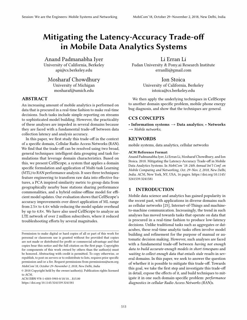
2.3.2 Ineffectiveness ofGlobalModel. A common ap-proach in applying ML on a dataset is to consider the datasetas a single entity and build one model over the entire data.However, base stations in a cellular network exhibit differ-ent characteristics. This renders the use of a global modelineffective. To illustrate this problem, we conducted an ex-periment where the goal is to build a model for call drops inthe network (similar to [26]) using information in our traces.Specifically, we build a decision tree model using an hourworth of data to ensure sufficient data for the algorithm toproduce statistically significant results. Figure 2a shows theresult of this experiment, where we see that the global model


515

0 20 40 60 80

100 120 140

Global Local Local (Stale) Spatial

Model

Accuracy (%)Validation Error (%)

(a) A single global model incurs poor ac-curacy. Local model is the best, but re-quires enough data to build and frequentupdates (otherwise staleness affects itsperformance). Combining data from ge-ographically nearby base stations resultsin a reduction in accuracy.

��

� � � � � ��

��

��

��

(b) Distribution of data collected by basestations under various data collection la-tencies. It take approximately an hourfor a vast majority of the base stations tocollect data to build statistically signifi-cant models.

��

��

��

��

��

��

� � � � � ��

��

��

��

(c) For building local models, it may notbe possible to simply wait for enoughdata. A random forestmodel (Alg 1) gainsfrom more data, but a lasso regressionmodel (Alg2) degrades with more datadue to temporal effects.

Figure 2: Simply applyingML forRANperformance diagnosis results in a fundamental trade-off between latency and accuracy.

achieves poor accuracy and high variance. This underlinesthe heterogeneity in the characteristics of base stations andhence the ineffectiveness of global models.

2.3.3 Latency/Accuracy Issues with Local Models.The alternative to a single global model is to build a modelfor every base station. We evaluate this approach by repeat-ing the last experiment, but this time segregating the datafor every base station and building an independent modelfor each. The results of this experiment is shown in fig. 2a,which indicates that local models are far superior, with upto 20% more accuracy while showing much lower variance.It is natural to think of a per base station model as the

final solution to this problem. However, this approach hasissues too. Due to the difference in characteristics of thebase stations, the amount of data they collect in a giventime interval varies vastly. Thus, in small intervals, they maynot generate enough data to produce statistically significantresults. Figure 2b shows the distribution of the amount ofdata generated by these base stations under different datacollection latencies. It shows that at small intervals (e.g.,under 10minutes), most base stations do not generate enoughdata, and that it takes about an hour for all quartiles of basestations to log reasonable number of records.

To illustrate the effect of this discrepancy, we conduct an-other experiment. We use two machine learning algorithms—a random forest model to predict connection drops (Alg1), and a lasso regression model using stochastic gradientdescent to predict the throughput (Alg 2)—at various datacollection latencies. These two algorithms represent someof the commonly used models from the broad categories ofclassification and regression. The result of this experiment isshown in fig. 2c. The behavior of Alg 1 is obvious; as it getsmore data its accuracy improves due to the slow varyingnature of the underlying causes of failures. After an hour

latency1, it is able to reach a respectable accuracy. However,the second algorithm’s accuracy initially seems to improvewith more data, but falls quickly. This is counterintuitivein normal settings, but the explanation lies in the spatio-temporal characteristics of cellular networks. Many of theperformance metrics exhibit high temporal variability, andthus need to be analyzed in smaller intervals. Thus, in modelslike that in Alg 2, it is not enough to just “wait” for enoughdata to be collected, and hence local modeling is ineffective.

2.3.4 Need forModelUpdates. An obvious, but flawedconclusion from our previous experiment is that models sim-ilar to that built by Alg 1 would work after the data collectionlatency (of an hour) has been incurred once. Put differently,can we just use historic data? In any application of ML, mod-els need to be updated to retain their performance. This istrue in cellular networks too, where temporal variations af-fect the performance of themodel. To depict this, we repeatedthe experiment where we built per base station decision treemodel for call drops. However, instead of training and testingon parts of the same dataset, we train on an hours worthof data, and test it on the next hour. Figure 2a shows thatthe accuracy drops by 12% with a stale model (because themodel built using historic data is no longer valid). Thus, it isimportant to keep the model fresh by incorporating incom-ing data and removing old data. Such sliding updates to MLmodels in a general setting is difficult due to the overheadsin retraining them from scratch. To add to this, cellular net-works consist of several thousands of base stations. Thus, aper base station approach requires creating and updating ahuge amount of models (e.g., our network consisted of over13000 base stations). This makes scaling hard.

2.3.5 Why not Spatial/Temporal Partitioning? Ourexperiments point towards the need for obtaining enough1Such high latencies may not be acceptable in many scenarios.


516

CellScope

Domain-Specific MTL

Gradient Boosted Trees

RAN Performance Analyzer

ML Lib

Bearer Level Trace

Dashboards

Self-Organizing Networks (SON)

Throughput Drop

Feature Engineering

PCA-Based Similarity Grouping

Streaming

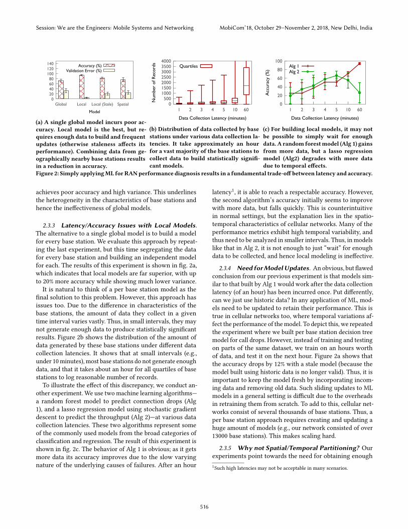
Figure 3: CellScope System Architecture.

data for ML algorithms to produce statistically significantresults with low latency. The obvious solution to combatingthis trade-off is to intelligently combine data from multiplebase stations. It is intuitive to think of this as a spatial par-titioning problem, since base stations in the real world aregeographically separated. Thus, it is reasonable to assumethat a spatial partitioner which combines data from basestations within a geographical region must be able to givegood results. Unfortunately, this isn’t the case which we mo-tivate using a simple example. Consider two base stations,one situated at the center of times square in New York andthe other a mile away at a residential area. Using a spatialpartitioning scheme that divides the space into equal sizedplanes would likely result in combining data from these basestations. However, this is not desirable because of the differ-ence in characteristics of these base stations2. We illustratethis using the drop modeling experiment as before. Figure 2ashows the performance where we combine data from nearbybase stations using a simple grid partitioner, and then builda model in each of the partitions. The result shows that thistechnique is only slightly better compared to a single globalmodel. We evaluate other spatial partitioning schemes in §6.

3 CELLSCOPE OVERVIEWWe now present our solution, CellScope, which mitigatesthe latency-accuracy trade-off using a domain-specific for-mulation and application of Multi-Task Learning (MTL).

3.1 Problem StatementCellScope’s ultimate goal is to enable fast and accurate RANperformance diagnosis by resolving the trade-off between datacollection latency and the achieved accuracy. The key diffi-culty arises from the fundamental trade-off between havingnot enough data to build accurate-enough models in shorttimespans and waiting to collect enough data that entails staleresults. Additionally, CellScope must also support efficientmodifications to the learned models to account for the tem-poral nature of our setting to avoid data and model staleness.2In our measurements, a base station in a highly popular spot serves morethan 300 UEs and carries multiple times uplink / downlink traffic comparedto another base station situated just a mile from it that serves only 50 UEs.

3.2 Architectural OverviewFigure 3 shows the high-level architecture of CellScope,which consists of the following key components:Input data: CellScope uses measurement traces that arereadily available in modern cellular networks (§2.1). Basestations collect traces independently and send them to the as-sociated MME, which merges records if required and uploadsthem to a data center.3Feature engineering:Next, CellScope uses domain knowl-edge to transform the raw data and construct a set of fea-tures amenable to learning (e.g., computing interference ra-tios)(§4.1). We also leverage protocol details and algorithms(e.g., link adaptation in the physical layer).Domain-specific MTL: CellScope uses a domain specificformulation and application of MTL that allows it to performaccurate diagnosis while updating models efficiently (§4.2).Data partitioner: To enable correct application of MTL,CellScope implements a partitioner based on a similarityscore derived from Principal Component Analysis (PCA) andgeographical distance (§4.3). The partitioner segregates datato be analyzed into independent sets and produces a smallerco-located set relevant to the underlying analysis. This alsominimizes the need to shuffle data during training.RANperformance analyzer: This component binds every-thing together to build diagnosis modules. It leverages theMTL component and uses appropriate techniques to buildcall drop and throughput models. We discuss our experienceof applying these techniques to a live LTE network in §7.This component can be easily replaced to extend CellScopeto a new domain, as we show in §8.Output: Finally, CellScope can output analytics results toexternal modules such as RAN performance dashboards. Itcan also provide inputs to Self-Organizing Networks (SON).

4 MITIGATING LATENCY ACCURACYTRADE-OFF

In this section, we present how CellScope mitigates thetrade-off between latency and accuracy. We first discuss ahigh-level overview of RAN specific feature engineeringthat prepares the data for learning (§ 4.1). Next, we describeCellScope’s MTL formulation (§ 4.2), and how it lets us buildfast, accurate and incremental models. Then, we explain howCellScope achieves grouping that captures commonalitiesamong base stations using a novel PCA based partitionerthat makes application of MTL possible (§ 4.3).

4.1 Feature EngineeringFeature engineering, the process of transforming the rawinput data to a set of features that can be effectively utilized3The transfer of traces to a data center is not fundamental. ExtendingCellScope to do geo-distributed learning in a future work.


517

by machine learning algorithms, is a fundamental part of MLapplications [58]. Generally carried out by domain experts,it is often the first step in ML.In CellScope, the network measurement data contains

several hundreds of fields (§2). These fields range from sim-ple bearer identification information to fields associated withLTE network procedures. Unfortunately, many of these fieldsare not suitable for model building as it is. Additionally, sev-eral fields are collected in a format that utilizes a compactrepresentation. Finally, these records are not self-contained,and multiple records may need to be “joined” to create afeature for a certain procedure. We use simple feature engi-neering to obtain fields that can be used in ML algorithms.As an example, for modeling connection drop rates, we useblock error rate (BLER) as a feature. However, the recordsdo not directly provide this value, thus it is computed us-ing the block transfer information. Similarly, for throughputmodeling, the downlink and uplink throughput values arecomputed using the amount of physical resource blocks al-located and the transfer time. While we depend on manualfeature engineering in this work (automating this is part ofour future work), not all fields need to be feature engineered.Further, we found that the engineered fields can be usedacross several ML algorithms.

4.2 Multi-Task LearningThe latency-accuracy trade-off makes it hard to achieve bothlow latency and high accuracy in ML tasks (§2). The ideal-case scenario in CellScope is if infinite amount of data isavailable per base station with zero latency. In this scenario,we would have a learning task for each base station thatproduce a model as an output with the best achievable accu-racy. In reality, our setting has several tasks, each with itsown data. However, each task does not have enough datato produce models with acceptable accuracy in a given la-tency budget. This makes our setting an ideal candidate formulti-task learning (MTL), a research area in machine learn-ing that has been successful in many ML applications. Thekey idea behind MTL is to learn from other tasks by weaklycoupling their parameters so that the statistical efficiency ofmany tasks can be boosted [10, 11, 17, 50]. Specifically, if weare interested in building a model of the form

h(x) =m(f1(x), f2(x), ..., fk (x)) (1)

wherem is a model (e.g., to predict connection drop) com-posed of feature functions f1 through fk , then the traditionalMTL formulation, given dataset D = {(xi ,yi ,bsi ) : i =1, ...,n}, where xi ∈ Rd ,yi ∈ R and bsi denotes the ith basestation, is to learn

h(x) =mbs (f1(x), f2(x), ..., fk (x)) (2)

wherembs is a per base station model.

In this MTL formulation, the core assumption is a sharedstructure or dependency across each of the learning problems.Unfortunately, in our setting, the base stations do not sharea structure at a global level (§2). Due to their geographic sep-aration and the complexities of wireless signal propagation,the base stations share a spatio-temporal structure instead.Thus, we proposes a new domain-specific MTL formulation.

4.2.1 CellScope’s MTL Formulation. In order to ad-dress the difficulty in applying MTL due to the violationof task dependency assumption in RANs, we can leveragedomain-specific characteristics. Although independent learn-ing tasks (learning per base station) are not correlated witheach other, they exhibit specific non-random structure. Forexample, the performance characteristics of base stationsnearby are influenced by similar underlying features. Thus,we propose exploiting this knowledge to segregate learningtasks into groups of dependent tasks on which MTL canbe applied. MTL in the face of dependency violation hasbeen studied in the machine learning literature in the recentpast [20, 30]. However, they assume that each group has itsown set of features. This is not entirely true in our setting,where multiple groups may share most or all features but stillneed to be treated as separate groups. Furthermore, some ofthe techniques used for automatic grouping without a prioriknowledge are computationally intensive.

Assuming we can club learning tasks into groups, we canrewrite the MTL equation in eq. (2) as:

h(x) =mд(bs)(f1(x), f2(x), ..., fk (x)) (3)

wheremд(bs) is the per-base station model in group д. Wedescribe a simple technique to achieve this grouping basedon domain knowledge in § 4.3 and experimentally show thatjust grouping can achieve significant gains in §6.

In theory, the MTL formulation in eq. (3) should suffice forour purposes as it would perform much better by capturingthe inter-task dependencies using grouping. However, thisformulation still builds an independent model for each basestation. Building and managing a large amount of modelsleads to significant performance overhead and would im-pede our goal of scalability. Scalable application of MTL ina general setting is an active area of research in machinelearning [36], so we turn to problem-specific optimizationsto address this challenge.

The modelmд(bs) could be built using any class of learningfunctions. In this paper, we restrict ourselves to functions ofthe form F (x) = w ·x wherew is the weight vector associatedwith a set of features x . This simple class of function gives ustremendous leverage in using standard algorithms that caneasily be applied in a distributed setting, thus addressing thescalability issue. In addition to scalable model building, wemust also be able to update the built models fast. However,


518

machine learning models are typically hard to update in realtime. To address this challenge, we discuss a hybrid approachto building the models in our MTL setting next.

4.2.2 Hybrid Modeling for Fast Model Updates. Es-timation of the model in eq. (3) could be posed as an ℓ1regularized loss minimization problem [51]:

min∑

L(h(x : fbs ),y) + λ | |R(x : fbs )| | (4)

where L(h(x : fbs ),y) is a non-negative loss function com-posed of parameters for a particular base station, hence cap-turing the error in the prediction for it in the group, and λ > 0is a regularization parameter scaling the penalty R(x : fbs )for the base station. However, the temporal and streamingnature of the data means that the model must be refinedfrequently for minimizing staleness.

Fortunately, grouping provides us an opportunity to solvethis. Since the base stations are grouped into correlated taskclusters, we can decompose the features used for each basestation into a shared common set fc and a base station specificset fs . Thus, we can modify eq. (4) as minimizing∑ (∑

L(h(x : fs , fc ),y) + λ | |R(x : fs )| |

)+ λ | |R(x : fc )| |

(5)where the inner summation is over dataset specific to eachbase station. This separation gives us a powerful advantage.Since we grouped base stations, the feature set fs is minimal,and in most cases just a weight vector on the common featureset. Because the core common features do not change often,we need to update only the base station-specific parts in themodel frequently, while the common set can be reused. Thus,we end up with a hybrid offline-online model. Furthermore,the choice of our learning functions lets us apply stochasticmethods [45] which can be efficiently parallelized.

4.2.3 AnomalyDetectionUsingConceptDrift. A com-mon use case of learning tasks for RAN performance analysisis in detecting anomalies. For instance, an operator may beinterested in learning if there is a sudden increase in calldrops. At the simplest level, it is easy to answer this questionby monitoring the number of call drops at each base station.However, just a yes or no answer to such questions are sel-dom useful. If there is a sudden increase in drops, then it isuseful to understand if the issue affects a complete regionand its root cause.

Our MTL approach and the ability to do fast incrementallearning enables a better solution for anomaly detection anddiagnosis. Concept drift is a term used to refer the phenome-non where the underlying distribution of the training datafor a machine learning model changes [19]. CellScope lever-ages this to detect anomalies as concept drifts and proposesa simple technique for it. Since we process incoming data in

mini-batches (§5), each batch can be tested quickly on theexisting model for significant accuracy drops. An anomalyoccurring just at a single base station would be detected byone model, while one affecting a larger area would be de-tected by many. Once anomaly is detected, finding cause isas easy as updating the model and comparing it with the old.

4.3 Data Grouping for MTLHaving discussed CellScope’s MTL formulation, we nowturn our focus towards how CellScope achieves efficientgrouping of cellular datasets that enables accurate learn-ing. Our data partitioning is based on Principal ComponentAnalysis (PCA), a widely used technique in multivariate anal-ysis [37]. PCA uses an orthogonal coordinate transformationto map a given set of points into a new coordinate space.Each of the new subspaces are commonly referred to as aprincipal component. Since the coordinate space is smallerthan the original , PCA is used for dimensionality reduction.In their pioneering work, Lakhina et.al. [33] showed the

usefulness of PCA for network anomaly detection. Theyobserved that it is possible to segregate normal behavior andabnormal (anomalous) behavior using PCA—the principalcomponents explain most of the normal behavior while theanomalies are captured by the remaining subspaces. Thus,by filtering normal behavior, it is possible to find anomaliesthat may be otherwise undetected.While the most common usecase for PCA has been di-

mensionality reduction (in machine learning domains) oranomaly detection (in networking domain), we use it in anovel way, to enable grouping of datasets formulti-task learn-ing. Due to the lack of the ability to collect sufficient amountof data from individual base stations, detecting anomaliesin them will not yield results. However, the data would stillyield an explanation of normal behavior. We use this obser-vation to partition the dataset.

4.3.1 Notation. As bearer level traces are collected con-tinuously, we consider a buffer of bearers as a measurementmatrix A. Thus, A consists ofm bearer records, each havingn observed parameters making it anm×n time-series matrix.It is to be noted that n is in the order of a few 100 fields, whilem can be much higher depending on how long the bufferinginterval is. We enforce n to be fixed in our setting—everymeasurement matrix must contain n columns. To make thismatrix amenable to PCA analysis, we adjust the columnsto have zero mean. By applying PCA to any measurementmatrix A, we can obtain a set of k principal componentsordered by amount of data variance they capture.

4.3.2 PCA Similarity. It is intuitive to see that manymeasurement matrices may be formed based on different


519

criteria. Suppose we are interested in finding if two mea-surement matrices are similar. One way to achieve this isto compare the principal components of the two matrices.Krzanowski [32] describes such a Similarity Factor (SF ). Con-sider two matrices A and B having the same number ofcolumns, but not rows. The similarity factor between A andB is:

SF = trace(LM ′ML′) =k∑i=1

k∑j=1

cos2 θi j

where L,M are the first k principal components ofA and B re-spectively, and θi j is the angle between the ith component ofA and the jth component of B. The similarity factor considersall combinations of k components from both matrices.

4.3.3 CellScope’s Similarity Metric. Similarity in oursetting bears a slightly different meaning: we do not wantstrict similarity between measurement matrices, but onlysimilarity between corresponding principal components. Thisensures that algorithms will still capture the underlying ma-jor influences and trends in observation sets that are notexactly similar. So we propose a simpler metric.Consider two measurement matrices A and B as before,

whereA is of sizemA×n and B is of sizemB ×n. By applyingPCA on the matrices, we can obtain k principal componentsusing a heuristic. We obtain the first k components whichcapture 95% of the variance. From the PCA, we obtain theresulting weight vector, or loading, which is a n × k matrix:for each principal component in k , the loading describesthe weight on the original n features. Intuitively, this can beseen as a rough measure of the influence of each of the nfeatures on the principal components. The Euclidean distancebetween the corresponding loading matrices gives

SFCellScope =k∑i=1

d(ai ,bi ) =k∑i=1

n∑j=1

|ai j − bi j |

where a and b are the column vectors representing the load-ings for the corresponding principal components fromA andB. Thus, SFCellScope captures how closely the underlyingfeatures explain the variation in the data.

Due to the complex interactions between network compo-nents and the wireless medium, many of the performanceissues in RANs are geographically tied (e.g., congestionmighthappen in nearby areas, and drops might be concentrated)4.However, SFCellScope doesn’t capture this phenomenon be-cause it only considers similarity in normal behavior. Conse-quently, it is possible for anomaly detection algorithms tomiss geographically-relevant anomalies. To account for thisdomain-specific characteristic, we augment our similarity4Proposals for conducting geographically weighted PCA (GW-PCA) ex-ist [22], but they are not applicable since they assume a smooth decayinguser provided bandwidth function.

metric to also capture the geographical closeness by weigh-ing the metric by geographical distance between the twomeasurement matrices. Our final similarity metric is5

SFCellScope = wdistance(A,B) ×

k∑i=1

n∑j=1

|ai j − bi j |

4.3.4 Using SimilarityMetric for Partitioning. Withsimilaritymetric,CellScope can nowpartition bearer records.We first group the bearers into measurement matrices bysegregating them based on the cell on which the bearer orig-inated. The grouping is based on our observation that thecell is the lowest level at which an anomaly would mani-fest. We then create a graph G(V ,E) where the vertices arethe individual cell measurement matrices. An edge is drawnbetween two matrices if the SFCellScope between them isbelow a threshold. To compute SFCellScope , we simply usethe geographical distance between the cells as the weight.Once the graph has been created, we run connected com-ponents on this graph to obtain the partitions. The use ofconnected component algorithm is not fundamental, it isalso possible to use a clustering algorithm instead. For in-stance, a k-means clustering algorithm that could leverageSFCellScope to merge clusters would yield similar results.

4.3.5 ManagingPartitionsOver Time. One importantconsideration is managing group changes over time. To de-tect group changes, it is necessary to establish correspon-dence between groups across time intervals. Once this cor-respondence is established, CellScope’s hybrid modelingmakes it easy to accommodate changes. Due to the segre-gation of our model into common and base station specificcomponents, small changes to the group do not affect thecommon model. In these cases, we can simply bootstrap thenew base station using the common model, and then startlearning specific features. On the other hand, if there aresignificant changes to a group, then the common model mayno longer be valid, which is easy to detect using conceptdrift. In such cases, the offline model could be rebuilt.

4.4 SummaryWe now summarize how CellScope resolves the fundamen-tal trade-off between latency and accuracy. To cope with thefact that individual base stations cannot produce enough datafor learning in a given time budget, CellScope uses MTL.However, our datasets violate the assumption of learningtask dependencies. As a solution, we proposed a novel way ofusing PCA to group data into sets with the same underlyingperformance characteristics. Directly applying MTL on these5A similarity measure for multivariate time series is proposed in [55], butit is not applicable due to its stricter form and dependence on finding theright eigenvector matrices to extend the Frobenius norm.


520

groups would still be problematic in our setting due to theinefficiencies with model updates. To solve this, we proposeda new formulation for MTL which divides the model into anoffline and online hybrid. On this formulation, we proposedusing simple learning functions are amenable to incrementaland distributed execution. Finally, CellScope uses a simpleconcept drift detection to find and diagnose anomalies.

5 IMPLEMENTATIONWe have implemented CellScope on Spark [56]. We describeits API that exposes our commonality based grouping basedon PCA (§ 5.1), and implementation details on the hybridoffline-online MTL models (§ 5.2).

5.1 Data Grouping APICellScope’s grouping API is built on Spark Streaming [57],since the data arrives continuously, and we need to operateon this data in a streaming fashion. Spark Streaming alreadyprovides support for windowing functions on streams ofdata, thus we extended it with the three APIs in listing 1.

grouped = DStream.groupBySimilarityAndWindow(windowDuration, slideDuration)

reduced = DStream.reduceBySimilarityAndWindow(func, windowDuration, slideDuration)

joined = DStream.joinBySimilarityAndWindow(windowDuration, slideDuration)

Listing 1: Groping API

The APIs leverage the DStream abstraction provided bySpark Streaming. groupBySimilarityAndWindow takesthe buffered data from the last window duration, appliesthe similarity metric to produce outputs of grouped datasetsevery slide duration. reduceBySimilarityAndWindow al-lows an additional user defined associative reduction opera-tion on the grouped datasets. Finally, joinBySimilarity-AndWindow joins multiple streams using similarity.

5.2 Hybrid MTL ModelingWe use Spark’s machine learning library, MLlib [47] for im-plementing our hybrid MTL model. MLlib contains imple-mentation for many distributed learning algorithms. TheMTL formulation we presented in § 4.2 allows us to utilizethese existing models in our framework.In MTL, the tasks learn from each other. These tasks in

our setting consist of building a model,mд(bs) for each basestation in every group created by the PCA based grouping.In eq. (3), we presented our MTL formulation, and describeda simplified loss minimization method to estimate this model.Further, in eq. (5), we decomposed this into shared and basestation specific set, so the model mд(bs) is of the general

form h(x : fs , fc ),y). Since we restrict ourselves to learningfunctions of the formw ·x for this model, our model per basestation is simply a weight vector on the shared group model.This allows the usage of existing ensemble methods [14].Ensemblemethods usemultiple learning algorithms to obtainbetter performance. In our case, we use the ensemble methodto learn the shared group model. This can be done in manyways: we can directly employ existing ensemble methods, orwe can leverage multiple algorithms to be components of theensemble. However, unlike normal ensemble methods wherethe output is aggregated, we use the MTL approach of a taskper base station to learn the per-base station model. Thisis equivalent to a linear model on the individual ensemblecomponents, which gives us the weight vector.

Wemodified theMLLib implementation of Gradient BoostedTree (GBT) [18]. This implementation supports both classifi-cation and regression, and internally uses stochastic methods.We implement the group’s shared feature model using eitherthe GBT’s ensemble, or individual algorithms. As an exam-ple, for connection drop prediction, the shared model can beobtained using the standard ensembles such as the GBT itself,or random forests. Then, we use individual base station datato fit a linear model on the individual ensemble components.Note that it is not necessary to build the base model thisway—we could also use multiple learning methods as ensem-ble components. In the same example, our ensemble couldconsist of a combination of SVM and decision trees. Similarly,for throughput prediction, the shared model is built as anensemble of regression models—for instance, we may useone model for low throughput and another for high through-put, and each of these tasks could use a different standardlearning method. In this method, we can update the basestation specific weight vector in real time as data is streamedin, as we simply need to update the linear model. Further, thegroup specific model can be periodically retrained. One wayto do so is to simply add more models to the ensemble whennew data comes in. Our implementation allows weighingthe outcome to give more weights to the latest models.

6 EVALUATIONWe have evaluated CellScope through a series of experi-ments on real-world cellular traces from a live LTE networkin a large geographical area. Our results show that:• CellScope’s similarity based grouping provides up to 10%improvement in accuracy on its own compared to the bestspace partitioning scheme.

• With MTL, CellScope’s accuracy improvements rangefrom 2.5× to 4.4× over different collection latencies.

• Our hybrid online-offline model is able to reduce modelupdate times upto 4.8× and is able to learn changes in anonline fashion with no loss in accuracy.


521

��

��

��

��

��

��

��

(a) Grouping by itself is able to providesignificant gains. MTL provides furthergains.

��

��

��

��

��

��

��

��

��

��

��

��

��

��

��

��

��

��

(b) Grouping is not computationally in-tensive, even a days worth of data (with>500M records) can be easily grouped inunder a minute.

��

��

��

��

��

��

� � � � � ��

��

��

��

(c) CellScope achieves up to 2.5× accu-racy improvements in drop rate classifi-cation.

��

��

��

��

��

��

� � � � � ��

��

��

��

(d) Improvements in throughput regres-sion go up to 4.4×

��

��

��

��

��

(e) CellScope’s hyrid model allows effi-cient updates, and reduces update timeby up to 4.8×.

��

��

��

��

��

��

� � � � � ��

��

��

��

(f) Online training due to the hybridmodel helps avoid the loss in accuracydue to staleness of the model.

Figure 4: CellScope is able to achieve high accuracy while reducing the data collection latency.

Evaluation Setup:We use a private cluster of 20 machines,each consisting of 4 CPUs, 32GB RAM and 200GB hard disk.Dataset: We collected data from a major metro-area LTEnetwork for a time period of over 10 months. It serves over2 million active users and carries over 6TB traffic per hour.

6.1 Benefits of Similarity Based GroupingWe first attempt to answer the question "How much bene-fits do the similarity based grouping provide?". For this, weconducted two experiments, each with a different learning al-gorithm. The first experiment, detection of call drops, uses aclassification algorithm while the second, throughput predic-tion, uses a regression algorithm. We chose these to evaluatethe benefits in two different classes of algorithms. In boththese cases, we pick the data collection latency where theper base station model gives the best accuracy, which was 1hour for classification and 5 minutes for regression. In orderto compare the benefits of our grouping scheme alone, webuild a single model per group instead of applying MTL. Wecompare the accuracy obtained with three different spacepartitioning schemes. The first scheme (Spatial 1) just par-titions space into grids of equal size. The second (Spatial 2)uses a sophisticated space-filling curve based approach [25]that could create dynamically sized partitions. Finally, thethird (Spatial 3) creates partitions using base stations thatare under the same region. Figure 4a shows the results.

CellScope’s similarity grouping performs as good as theper base station model which gives the highest accuracy. Itis interesting to note the performance of spatial partitioningschemes which ranges from 75% to 80%. None of the spa-tial schemes come close to the similarity grouping results.This is because the drops are few, and concentrated. Spatialschemes club base stations not based on underlying dropcharacteristics, but only based on spatial proximity. Thiscauses the algorithms to underfit or overfit. Since our simi-larity based partitioner groups base stations using the dropcharacteristics, it is able to do as much as 17% better.

The benefits are even higher in the regression case. Here,the per base station model is unable to get enough data tobuild an accurate model and hence is only able to achievearound 66% accuracy. Spatial schemes are able to do slightlybetter than that. Our similarity based grouping emerges asa clear winner in this case with 77.3% accuracy. This resultdepicts the highly variable performance characteristics ofthe base stations, and the need to capture them for accuracy.These benefits do not come at the cost of computationaloverhead due to grouping. Figure 4b shows the overhead ofsimilarity based grouping on various dataset sizes.

6.2 Benefits of MTLNext, we characterize the benefits ofCellScope’s use of MTL.We repeated the experiment before, and apply MTL to the


522

grouped data to see if the accuracy improves compared tothe earlier approach of a single model per group. The resultsare presented in figure 4a. The ability of MTL to learn and im-prove models from other similar base stations’ data results inan increase in the accuracy. Over the benefits of grouping, wesee an improvement of 6% in the connection drop diagnosisexperiment, and 16.2% in the case of throughput predictionexperiment. The higher benefits in the latter comes fromCellScope’s ability to capture individual characteristics ofthe base station. This ability is not so crucial in the formerbecause of the limited variation in individual characteristics.

6.3 Combined BenefitsHere, we are interested in evaluating howCellScope handlesthe latency accuracy trade-off. We do the same classificationand regression experiments, but on different data collectionlatencies. We show the results from the classification andregression experiment in fig. 4c and fig. 4d, which comparesCellScope’s accuracy against a per base station model’s.When the opportunity to collect data at individual base

stations is limited, CellScope is able to leverage our MTLformulation to combine data from multiple base stations,and build customized models to improve the accuracy. Thebenefits of CellScope ranges up to 2.5× in the classificationexperiment, to 4.4× in the regression experiment. Lowerlatencies are problematic in the classification experimentdue to the extremely low probability of drops, while higherlatencies are a problem in the regression experiment due tothe temporal changes in performance.

6.4 Hybrid model benefitsFinally, we are interested in learning how much overhead itreduces during model updates, and if it do online learning.

To answer the first question, we conducted the followingexperiment: we considered three different data collectionlatencies: 10 minute, 1 hour and 1 day. We then learn a deci-sion tree model on this data in a tumbling window fashion.So for the 10 minute latency, we collect data for 10 minutes,then build a model, wait another 10 minutes to refine themodel and so on. We compare our hybrid model strategyto two different strategies: a naive approach which rebuildsthe model from scratch every time, and a better, strawmanapproach which reuses the last model, and makes changesto it. Both builds a single model while CellScope uses ourhybrid MTL model and only updates the online part of themodel. The results of this experiment is shown in figure 4e.The naive approach incurs the highest overhead, which

is obvious due to the need to rebuild the entire model fromscratch. The overhead increases with the increase in inputdata. The strawman approach, on the other hand, is able toavoid this heavy overhead. However, it still incurs overheads

with larger input because of its use of a single model whichrequires changes to many parts of the tree. CellScope incursthe least overhead, due to its use of multiple models. Whendata accumulates, it only needs to update a part of an existingtree, or build a new tree. This strategy results in a reductionof up to 2.2× to 4.8× in model building time for CellScope.To wrap up, we evaluated the performance of the hybrid

strategy on different data collection intervals. Here we areinterested in seeing if the hybrid model is able to adapt todata changes and provide reasonable accuracies. We use theconnection drop experiment again, but do it in a differentway. At different collection latencies, we build the model atthe beginning of the collection and use the model for the nextinterval. Hence, for the 1 minute latency, we build a modelusing the first minute data, and use the model for the secondminute (until the whole second minute has arrived). Theresults are shown in figure 4f. We see here that the per basestation model suffers an accuracy loss at higher latenciesdue to staleness, while CellScope incurs almost zero loss inaccuracy. This is because it doesn’t wait until the end of theinterval, and is able to incorporate data in real time.

7 REAL WORLD RAN ANALYSISWe now turn to the question of how could operators benefitfrom a system such as CellScope? We try to answer thisquestion in two ways: first, we try to evaluate what are thebenefits of automatic root-causing and how much effort isreduced for the operator because of this feature. Second, weevaluate CellScope’s ability to analyze in the wild.

7.1 Time Savings to the OperatorOperators spend several billions of dollars in diagnosingnetwork problems. Often, finding the cause of a networkproblem takes hours, or even days of effort. To evaluate howCellScope could cut down this effort, we collected networktrouble tickets from the operator. The operator logs ticketsat different levels, so we look at trouble tickets that wereinvestigated by domain experts using state-of-the-art toolssuch as datacubes. For each ticket where the operator hasnetwork data available, we used CellScope to diagnose theproblem. This way, we can evaluate the potential time sav-ings CellScope provides. We discuss four real trouble tickets,the time taken by CellScope is depicted in table 1.

7.1.1 Throughput Degradation After Upgrade. This ticketreported that a number of users experienced degraded net-work throughput after a network upgrade. In many cases,throughput decrease of up to 30% was observed. Since not allof the users saw this problem, the operator had to conductfield trials to find the root cause of the problem. We usedCellScope to model the throughput before and after theupgrade. Comparing the models, we noticed that a cluster of


523

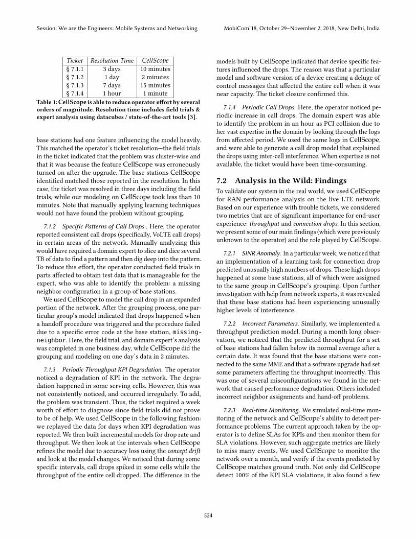
Ticket Resolution Time CellScope§ 7.1.1 3 days 10 minutes§ 7.1.2 1 day 2 minutes§ 7.1.3 7 days 15 minutes§ 7.1.4 1 hour 1 minute

Table 1:CellScope is able to reduce operator effort by severalorders of magnitude. Resolution time includes field trials &expert analysis using datacubes / state-of-the-art tools [3].

base stations had one feature influencing the model heavily.This matched the operator’s ticket resolution—the field trialsin the ticket indicated that the problem was cluster-wise andthat it was because the feature CellScope was erroneouslyturned on after the upgrade. The base stations CellScopeidentified matched those reported in the resolution. In thiscase, the ticket was resolved in three days including the fieldtrials, while our modeling on CellScope took less than 10minutes. Note that manually applying learning techniqueswould not have found the problem without grouping.

7.1.2 Specific Patterns of Call Drops . Here, the operatorreported consistent call drops (specifically, VoLTE call drops)in certain areas of the network. Manually analyzing thiswould have required a domain expert to slice and dice severalTB of data to find a pattern and then dig deep into the pattern.To reduce this effort, the operator conducted field trials inparts affected to obtain test data that is manageable for theexpert, who was able to identify the problem: a missingneighbor configuration in a group of base stations.

We used CellScope to model the call drop in an expandedportion of the network. After the grouping process, one par-ticular group’s model indicated that drops happened whena handoff procedure was triggered and the procedure faileddue to a specific error code at the base station, missing-neighbor. Here, the field trial, and domain expert’s analysiswas completed in one business day, while CellScope did thegrouping and modeling on one day’s data in 2 minutes.

7.1.3 Periodic Throughput KPI Degradation. The operatornoticed a degradation of KPI in the network. The degra-dation happened in some serving cells. However, this wasnot consistently noticed, and occurred irregularly. To add,the problem was transient. Thus, the ticket required a weekworth of effort to diagnose since field trials did not proveto be of help. We used CellScope in the following fashion:we replayed the data for days when KPI degradation wasreported. We then built incremental models for drop rate andthroughput. We then look at the intervals when CellScoperefines the model due to accuracy loss using the concept driftand look at the model changes. We noticed that during somespecific intervals, call drops spiked in some cells while thethroughput of the entire cell dropped. The difference in the

models built by CellScope indicated that device specific fea-tures influenced the drops. The reason was that a particularmodel and software version of a device creating a deluge ofcontrol messages that affected the entire cell when it wasnear capacity. The ticket closure confirmed this.

7.1.4 Periodic Call Drops. Here, the operator noticed pe-riodic increase in call drops. The domain expert was ableto identify the problem in an hour as PCI collision due toher vast expertise in the domain by looking through the logsfrom affected period. We used the same logs in CellScope,and were able to generate a call drop model that explainedthe drops using inter-cell interference. When expertise is notavailable, the ticket would have been time-consuming.

7.2 Analysis in the Wild: FindingsTo validate our system in the real world, we used CellScopefor RAN performance analysis on the live LTE network.Based on our experience with trouble tickets, we consideredtwo metrics that are of significant importance for end-userexperience: throughput and connection drops. In this section,we present some of ourmain findings (whichwere previouslyunknown to the operator) and the role played by CellScope.

7.2.1 SINRAnomaly. In a particular week, we noticed thatan implementation of a learning task for connection droppredicted unusually high numbers of drops. These high dropshappened at some base stations, all of which were assignedto the same group in CellScope’s grouping. Upon furtherinvestigationwith help from network experts, it was revealedthat these base stations had been experiencing unusuallyhigher levels of interference.

7.2.2 Incorrect Parameters. Similarly, we implemented athroughput prediction model. During a month long obser-vation, we noticed that the predicted throughput for a setof base stations had fallen below its normal average after acertain date. It was found that the base stations were con-nected to the same MME and that a software upgrade had setsome parameters affecting the throughput incorrectly. Thiswas one of several misconfigurations we found in the net-work that caused performance degradation. Others includedincorrect neighbor assignments and hand-off problems.

7.2.3 Real-time Monitoring. We simulated real-time mon-itoring of the network and CellScope’s ability to detect per-formance problems. The current approach taken by the op-erator is to define SLAs for KPIs and then monitor them forSLA violations. However, such aggregate metrics are likelyto miss many events. We used CellScope to monitor thenetwork over a month, and verify if the events predicted byCellScope matches ground truth. Not only did CellScopedetect 100% of the KPI SLA violations, it also found a few


524

0 20 40 60 80

100 120 140

Global Local Model OS

Model

Accuracy (%)Validation Error (%)

Figure 5: Other domains suffer from latency-accuracy trade-off. Here, we see the problem in the domain of energy debug-ging formobile devices. Grouping by phonemodel or phoneoperating system does not give benefits.

issues that were missed by the KPI based monitoring system,and later logged as trouble tickets.

7.2.4 Measurement Error. We also found problems in net-work measurements. Specifically, during initial deploymenttrials of CellScope, we noticed that using the feature engi-neered field of block error rate resulted in poor accuracy. Thereason for this was an uninitialized field in the measurementrecord logger, which resulted in random values.

8 EXTENDING CELLSCOPE TO A NEWDOMAIN

To show the generality of the techniques presented in thispaper, we now apply these techniques to a new domain:energy anomaly detection in mobile phones [35]. We obtaineda dataset of measurements from approximately 800,000 usersobtained using the Carat app. The goal here is to suggestactions to users that help improve their battery life. This canbe done by building a battery usage model for each user.

Data: The Carat app periodically collects a variety of datafrom the mobile phone it is running on, including the phonemodel, version of the operating system, the state of the bat-tery, the CPU and memory utilization and the applicationsthat are running. We use these fields to build a ML modelthat predicts the battery drain rate for a user. Using thismodel, it is possible to point out potential application thatare responsible for an increased battery drain.

Latency-Accuracy Trade-off: For users signing up forthe Carat app, it is desirable to provide suggestions as soonas possible. However, currently, it takes several weeks forthe app to collect enough data for a new user. Figure 5 showsthe results of building a model for suggesting apps that arebugs for a particular user once enough data has been col-lected. It can be seen that a per-user model (denoted Local)works the best, but at the cost of latency. The local model

0

20

40

60

80

100

1 2 3 4 5 10

Acc

urac

y (%

)

Data Collection Latency (days)

Per userCellScope

Figure 6: CellScope’s techniques can easily be extended tonew domains, and can benefit them. Here, using our tech-niques, models built are usable immediately while withoutCellScope, Carat [35] takes more than a week to build amodel that is usable.

performs poorly until enough data has been collected as de-picted in fig. 6. A global model can be built immediately, buthas poor accuracy. It is intuitive to think of grouping userswho have the same model device together, or same operatingsystem together. However, these grouping (denoted Modeland OS) does not yield significant benefits. Further, as peopleinstall/uninstall apps, the models need to be updated. Thismake the domain ideal for testing CellScope’s techniques.

Extending Similarity Metric and MTL:. To extend ourtechniques to a new domain, we need to (i) customize thesimilarity metric (used for grouping) to the domain underconsideration, and (ii)modify the MTL formulation in eq. (5)for this domain. In the cellular networks domain, our simi-larity metric was weighted by geographic distance betweenbase stations. However, geographic distance does not havean effect here. From fig. 5, we notice that device model andoperating system also do not make much difference either.Intuitively, the subset of apps common between the usersshould provide better results. However, just that alone is notenough as usage patterns vary across users with similar apps.The Carat dataset provides enough information to determinethe number of times each app is active, which is roughly anindicator of the usage pattern for the user. We use that toderive usage similarity between users, uusaдe(A,B) , and utilizethat to form the similarity metric:

SFCellScope = uusaдe(A,B) ×k∑i=1

n∑j=1

|ai j − bi j |

The MTL formulation remains the same as in eq. (5), wesimply replace fs with per-user features fu .We implemented a Mobile Energy Diagnosis module in

CellScope at the same level as the RAN Performance Ana-lyzer in fig. 3 that uses our modified similarity metric andMTL formulation. We then applied the grouping and learn-ing to the measurement data we obtained to build a model


525

for suggesting bugs to a new user. The results are shownin fig. 6 which shows the accuracy of models built with (de-noted CellScope) and without CellScope (denoted per-user)starting from the day a user installs Carat. We see that on theday of signing up, the accuracy of the model built withoutusing CellScope is unusable. This is intuitive, since only afew samples have been sent by the new user’s device. Overtime, the user sends enough data and the accuracy improves.However, it takes over a week for Carat to offer usable sug-gestions to a new user. In contrast, with CellScope, we areable to build models that are immediately usable, and Caratcan begin offering suggestions on day 1.

9 RELATEDWORKMonitoring andTroubleshooting. Networkmonitoring

and troubleshooting has been an active area of research inboth wired networks [21, 28, 54] and wireless networks [3,4, 13, 16]. These techniques do not employ machine learningfor troubleshooting. Systems targeting RAN [4, 16] typicallymonitor aggregate KPIs and per-bearer records separately.Their root cause analysis of KPI problems correlates withaggregation air interface metrics such as SINR histogramsand configuration data. Because these systems rely on tradi-tional database technologies, it is hard for them to providefine-grained prediction based on bearer models. Recent re-search [25] and commercial offerings [6] have looked at theproblem of scalable cellular network analytics by leveragingbig data frameworks. However, they do not support learn-ing tasks. In contrast, CellScope focuses on scalable andaccurate application of machine learning in such domains.

Self-Organizing Networks (SON). The goal of SON [1]is to make the network capable of self-configuration (e.g.automatic neighbor list configuration) and self-optimization.CellScope’s techniques can provide the necessary diagnos-tics capabilities for assisting SON.

Modeling and Diagnosis Techniques. Problem diagno-sis in cellular networks has been explored extensively in theliterature in various forms [9, 23, 26, 34, 39, 49]. The focusof these has either been detecting faults or finding the rootcause of failures. A vast majority of such techniques dependon aggregate information and correlation based fault de-tection. [26] discusses the shortcomings of using aggregateKPIs, and propose the use of fine-grained information. Somestudies have focused on understanding the interaction ofapplications and cellular networks [24, 27, 38, 40, 52]. Theseare largely orthogonal to our work.

Finally, some recent proposals leverage the use of ML forspecific tasks. In [49], the authors discuss the use of ML toolsin predicting impending call drops and its duration. A proba-bilistic system for auto-diagnosing faults in RAN is presented

in [9]. It uses KPIs as inputs to the model. [8] shows thatimproving signal-to-noise ratio, decreasing load and reduc-ing handovers in cellular networks can improve web qualityof experience by using ML to model the influence of radionetwork characteristics on user experience metrics. Our pre-vious work [26] proposed the use of simple, explainable MLmodels towards the quest of automating RAN problem de-tection and diagnosis, and discussed several challenges inleveraging ML. In this paper, we present techniques that cansolve the challenges in leveraging ML in many domains.

Multi-Task Learning. MTL builds on the idea that re-lated tasks can learn from each other to achieve better sta-tistical efficiency [10, 11, 17, 50]. Since the assumption oftask relatedness do not hold in many scenarios, techniquesto automatically cluster tasks have been explored in thepast [20, 30]. However, these techniques consider tasks asblack boxes and hence cannot leverage domain specific struc-ture. CellScope proposes a hybrid offline-online MTL for-mulation on domain-specific grouping of tasks based on theunderlying performance characteristics.

10 CONCLUSIONThe practicality of real-time mobile data analytics in manydomains is impeded by a fundamental trade-off between datacollection latency and analysis accuracy. In this paper, wefirst exposed this trade-off using the domain of cellular net-works RAN. We presented CellScope to resolve this trade-off by applying a domain specific formulation of MTL. Toapply MTL effectively, CellScope proposed a novel PCA in-spired similarity metric that groups data from geographicallynearby base stations sharing performance commonalities. Fi-nally, it also incorporates a hybrid online-offline model forefficient model updates. Our evaluations show significantbenefits. We have also used CellScope to analyze a live LTEnetwork, where it could offer significant reduction in trou-bleshooting efforts. We then explored the generality of ourtechniques by applying them to a new domain, energy anom-aly diagnosis in smartphones. We show that extending ourgrouping and learning techniques to a new domain is easyand effective. Thus we believe our proposals form a solidframework for mitigating the effects of latency-accuracytrade-off in real-time mobile data analytics systems.

ACKNOWLEDGMENTSWe sincerely thank all MobiCom reviewers and our shep-herd for their valuable feedback. In addition to NSF CISEExpeditions Award CCF-1730628, this research is supportedby gifts from Alibaba, Amazon Web Services, Ant Financial,Arm, CapitalOne, Ericsson, Facebook, Google, Huawei, In-tel, Microsoft, Scotiabank, Splunk and VMware. MosharafChowdhury is supported by NSF grant CNS-1563095.


526

REFERENCES[1] 3gpp. [n. d.]. Self-Organizing Networks SON Policy Network Resource

Model (NRM) Integration Reference Point (IRP). http://www.3gpp.org/ftp/Specs/archive/32_series/32.521/.

[2] Bhavish Aggarwal, Ranjita Bhagwan, Tathagata Das, SiddharthEswaran, Venkata N. Padmanabhan, and Geoffrey M. Voelker. 2009.NetPrints: diagnosing home network misconfigurations using sharedknowledge. In Proceedings of the 6th USENIX symposium on Net-worked systems design and implementation (NSDI’09). USENIX Associ-ation, Berkeley, CA, USA, 349–364. http://dl.acm.org/citation.cfm?id=1558977.1559001

[3] Alcatel Lucent. 2013. 9900 Wireless Network Guardian. http://www.alcatel-lucent.com/products/9900-wireless-network-guardian.

[4] Alcatel Lucent. 2014. 9959 Network PerformanceOptimizer. http://www.alcatel-lucent.com/products/9959-network-performance-optimizer.

[5] Alcatel Lucent. 2014. Alcatel-Lucent Motive Big Network Analyticsfor service creation. http://resources.alcatel-lucent.com/?cid=170795.

[6] Alcatel Lucent. 2014. Motive Big Network Analytics. http://www.alcatel-lucent.com/solutions/motive-big-network-analytics.

[7] Paramvir Bahl, Ranveer Chandra, Albert Greenberg, Srikanth Kandula,David A. Maltz, and Ming Zhang. 2007. Towards Highly ReliableEnterprise Network Services via Inference of Multi-level Dependencies.In Proceedings of the 2007 Conference on Applications, Technologies,Architectures, and Protocols for Computer Communications (SIGCOMM’07). ACM, New York, NY, USA, 13–24. https://doi.org/10.1145/1282380.1282383

[8] Athula Balachandran, Vaneet Aggarwal, Emir Halepovic, Jeffrey Pang,Srinivasan Seshan, Shobha Venkataraman, and He Yan. 2014. ModelingWeb Quality-of-experience on Cellular Networks. In Proceedings ofthe 20th Annual International Conference on Mobile Computing andNetworking (MobiCom ’14). ACM, New York, NY, USA, 213–224. https://doi.org/10.1145/2639108.2639137

[9] Raquel Barco, Volker Wille, Luis Díez, and Matías Toril. 2010. Learn-ing of Model Parameters for Fault Diagnosis in Wireless Networks.Wirel. Netw. 16, 1 (Jan. 2010), 255–271. https://doi.org/10.1007/s11276-008-0128-z

[10] Jonathan Baxter. 2000. A Model of Inductive Bias Learning. J. Artif.Int. Res. 12, 1 (March 2000), 149–198. http://dl.acm.org/citation.cfm?id=1622248.1622254

[11] Richard Caruana. 1993. Multitask Learning: A Knowledge-BasedSource of Inductive Bias. In Proceedings of the Tenth InternationalConference on Machine Learning. Morgan Kaufmann, 41–48.

[12] Ira Cohen, Moises Goldszmidt, Terence Kelly, Julie Symons, and Jef-frey S. Chase. 2004. Correlating Instrumentation Data to System States:A Building Block for Automated Diagnosis and Control. In Proceedingsof the 6th Conference on Symposium on Opearting Systems Design &Implementation - Volume 6 (OSDI’04). USENIX Association, Berkeley,CA, USA, 16–16. http://dl.acm.org/citation.cfm?id=1251254.1251270

[13] Chuck Cranor, Theodore Johnson, Oliver Spataschek, and VladislavShkapenyuk. 2003. Gigascope: a stream database for network applica-tions. In Proceedings of the 2003 ACM SIGMOD international conferenceon Management of data (SIGMOD ’03). ACM, New York, NY, USA,647–651. https://doi.org/10.1145/872757.872838

[14] Thomas G Dietterich. 2000. Ensemble methods in machine learning.In Multiple classifier systems. Springer, 1–15.

[15] Ericsson. 2012. Ericsson RAN Analyzer Overview. http://www.optxview.com/Optimi_Ericsson/RANAnalyser.pdf.

[16] Ericsson. 2014. Ericsson RAN Analyzer. http://www.ericsson.com/ourportfolio/products/ran-analyzer.

[17] Theodoros Evgeniou andMassimiliano Pontil. 2004. RegularizedMulti–task Learning. In Proceedings of the Tenth ACM SIGKDD International

Conference on Knowledge Discovery and Data Mining (KDD ’04). ACM,New York, NY, USA, 109–117. https://doi.org/10.1145/1014052.1014067

[18] Jerome H Friedman. 2001. Greedy function approximation: a gradientboosting machine. Annals of statistics (2001), 1189–1232.

[19] João Gama, Indre Žliobaite, Albert Bifet, Mykola Pechenizkiy, andAbdelhamid Bouchachia. 2014. A Survey on Concept Drift Adaptation.ACM Comput. Surv. 46, 4, Article 44 (March 2014), 37 pages. https://doi.org/10.1145/2523813

[20] Pinghua Gong, Jieping Ye, and Changshui Zhang. 2012. Robust Multi-task Feature Learning. In Proceedings of the 18th ACM SIGKDD Interna-tional Conference on Knowledge Discovery and Data Mining (KDD ’12).ACM, New York, NY, USA, 895–903. https://doi.org/10.1145/2339530.2339672

[21] Nikhil Handigol, Brandon Heller, Vimalkumar Jeyakumar, David Maz-ières, and Nick McKeown. 2014. I Know What Your Packet Did LastHop: Using Packet Histories to Troubleshoot Networks. In Proceed-ings of the 11th USENIX Conference on Networked Systems Design andImplementation (NSDI’14). USENIX Association, Berkeley, CA, USA,71–85. http://dl.acm.org/citation.cfm?id=2616448.2616456

[22] Paul Harris, Chris Brunsdon, and Martin Charlton. 2011. Geographi-cally weighted principal components analysis. International Journal ofGeographical Information Science 25, 10 (2011), 1717–1736.

[23] Chi-YaoHong,MatthewCaesar, NickDuffield, and JiaWang. 2012. Tire-sias: Online Anomaly Detection for Hierarchical Operational NetworkData. In Proceedings of the 2012 IEEE 32Nd International Conference onDistributed Computing Systems (ICDCS ’12). IEEE Computer Society,Washington, DC, USA, 173–182. https://doi.org/10.1109/ICDCS.2012.30

[24] Junxian Huang, Feng Qian, Yihua Guo, Yuanyuan Zhou, Qiang Xu,Z. Morley Mao, Subhabrata Sen, and Oliver Spatscheck. 2013. AnIn-depth Study of LTE: Effect of Network Protocol and ApplicationBehavior on Performance. In Proceedings of the ACM SIGCOMM 2013Conference on SIGCOMM (SIGCOMM ’13). ACM, New York, NY, USA,363–374. https://doi.org/10.1145/2486001.2486006

[25] Anand Iyer, Li Erran Li, and Ion Stoica. 2015. CellIQ : Real-TimeCellularNetwork Analytics at Scale. In 12th USENIX Symposium on NetworkedSystems Design and Implementation (NSDI 15). USENIX Association,Oakland, CA, 309–322. https://www.usenix.org/conference/nsdi15/technical-sessions/presentation/iyer

[26] Anand Padmanabha Iyer, Li Erran Li, and Ion Stoica. 2017. AutomatingDiagnosis of Cellular Radio Access Network Problems. In Proceedingsof the 23rd Annual International Conference on Mobile Computing andNetworking (MobiCom ’17). ACM, New York, NY, USA, 79–87. https://doi.org/10.1145/3117811.3117813

[27] Haiqing Jiang, Yaogong Wang, Kyunghan Lee, and Injong Rhee. 2012.Tackling Bufferbloat in 3G/4G Networks. In Proceedings of the 2012ACM Conference on Internet Measurement Conference (IMC ’12). ACM,NewYork, NY, USA, 329–342. https://doi.org/10.1145/2398776.2398810

[28] Srikanth Kandula, Ratul Mahajan, Patrick Verkaik, Sharad Agarwal,Jitendra Padhye, and Paramvir Bahl. 2009. Detailed diagnosis in enter-prise networks. In Proceedings of the ACM SIGCOMM 2009 conferenceon Data communication (SIGCOMM ’09). ACM, New York, NY, USA,243–254. https://doi.org/10.1145/1592568.1592597

[29] Gunjan Khanna, Mike Yu Cheng, Padma Varadharajan, Saurabh Bagchi,Miguel P. Correia, and Paulo J. Veríssimo. 2007. Automated Rule-Based Diagnosis Through a Distributed Monitor System. IEEE Trans.Dependable Secur. Comput. 4, 4 (Oct. 2007), 266–279. https://doi.org/10.1109/TDSC.2007.70211

[30] Seyoung Kim and Eric P. Xing. 2010. Tree-Guided Group Lasso forMulti-Task Regression with Structured Sparsity. Intenational Confer-ence on Machine Learning (ICML) (2010).


527

http://www.3gpp.org/ftp/Specs/archive/32_series/32.521/

http://www.3gpp.org/ftp/Specs/archive/32_series/32.521/

http://dl.acm.org/citation.cfm?id=1558977.1559001


http://www.alcatel-lucent.com/products/9900-wireless-network-guardian

http://www.alcatel-lucent.com/products/9900-wireless-network-guardian

http://www.alcatel-lucent.com/products/9959-network-performance-optimizer

http://www.alcatel-lucent.com/products/9959-network-performance-optimizer

http://resources.alcatel-lucent.com/?cid=170795

http://www.alcatel-lucent.com/solutions/motive-big-network-analytics

http://www.alcatel-lucent.com/solutions/motive-big-network-analytics

https://doi.org/10.1145/1282380.1282383

https://doi.org/10.1145/1282380.1282383

https://doi.org/10.1145/2639108.2639137

https://doi.org/10.1145/2639108.2639137

https://doi.org/10.1007/s11276-008-0128-z

https://doi.org/10.1007/s11276-008-0128-z




https://doi.org/10.1145/872757.872838

http://www.optxview.com/Optimi_Ericsson/RANAnalyser.pdf

http://www.optxview.com/Optimi_Ericsson/RANAnalyser.pdf

http://www.ericsson.com/ourportfolio/products/ran-analyzer

http://www.ericsson.com/ourportfolio/products/ran-analyzer

https://doi.org/10.1145/1014052.1014067

https://doi.org/10.1145/2523813

https://doi.org/10.1145/2523813

https://doi.org/10.1145/2339530.2339672

https://doi.org/10.1145/2339530.2339672


https://doi.org/10.1109/ICDCS.2012.30

https://doi.org/10.1109/ICDCS.2012.30

https://doi.org/10.1145/2486001.2486006

https://www.usenix.org/conference/nsdi15/technical-sessions/presentation/iyer

https://www.usenix.org/conference/nsdi15/technical-sessions/presentation/iyer

https://doi.org/10.1145/3117811.3117813

https://doi.org/10.1145/3117811.3117813

https://doi.org/10.1145/2398776.2398810

https://doi.org/10.1145/1592568.1592597

https://doi.org/10.1109/TDSC.2007.70211

https://doi.org/10.1109/TDSC.2007.70211

[31] Tim Kraska, Ameet Talwalkar, John C. Duchi, Rean Griffith, Michael J.Franklin, and Michael I. Jordan. 2013. MLbase: A Distributed Machine-learning System. In CIDR. http://www.cidrdb.org/cidr2013/Papers/CIDR13_Paper118.pdf

[32] WJ Krzanowski. 1979. Between-groups comparison of principal com-ponents. J. Amer. Statist. Assoc. 74, 367 (1979), 703–707.

[33] Anukool Lakhina, Mark Crovella, and Christophe Diot. 2004. Diag-nosing Network-wide Traffic Anomalies. In Proceedings of the 2004Conference on Applications, Technologies, Architectures, and Protocolsfor Computer Communications (SIGCOMM ’04). ACM, New York, NY,USA, 219–230. https://doi.org/10.1145/1015467.1015492

[34] Yan Liu, Jing Zhang, M. Jiang, D. Raymer, and J. Strassner. 2008. Amodel-based approach to adding autonomic capabilities to networkfault management system. In Network Operations and ManagementSymposium, 2008. NOMS 2008. IEEE. 859–862. https://doi.org/10.1109/NOMS.2008.4575232

[35] Adam J. Oliner, Anand P. Iyer, Ion Stoica, Eemil Lagerspetz, and SasuTarkoma. 2013. Carat: Collaborative Energy Diagnosis for MobileDevices. In Proceedings of the 11th ACM Conference on Embedded Net-worked Sensor Systems (SenSys ’13). ACM, New York, NY, USA, Article10, 14 pages. https://doi.org/10.1145/2517351.2517354

[36] Yan Pan, Rongkai Xia, Jian Yin, and Ning Liu. 2015. A Divide-and-Conquer Method for Scalable Robust Multitask Learning. NeuralNetworks and Learning Systems, IEEE Transactions on 26, 12 (Dec 2015),3163–3175. https://doi.org/10.1109/TNNLS.2015.2406759

[37] K. Pearson. 1901. On lines and planes of closest fit to systems of pointsin space. Philos. Mag. 2, 6 (1901), 559–572.

[38] Feng Qian, Zhaoguang Wang, Alexandre Gerber, Zhuoqing Mao, Sub-habrata Sen, and Oliver Spatscheck. 2011. Profiling Resource Us-age for Mobile Applications: A Cross-layer Approach. In Proceed-ings of the 9th International Conference on Mobile Systems, Applica-tions, and Services (MobiSys ’11). ACM, New York, NY, USA, 321–334.https://doi.org/10.1145/1999995.2000026

[39] Sudarshan Rao. 2006. Operational Fault Detection in Cellular WirelessBase-stations. IEEE Trans. on Netw. and Serv. Manag. 3, 2 (April 2006),1–11. https://doi.org/10.1109/TNSM.2006.4798311

[40] Sanae Rosen, Haokun Luo, Qi Alfred Chen, Z. Morley Mao, Jie Hui,Aaron Drake, and Kevin Lau. 2014. Discovering Fine-grained RRC StateDynamics and Performance Impacts in Cellular Networks. In Proceed-ings of the 20th Annual International Conference on Mobile Computingand Networking (MobiCom ’14). ACM, New York, NY, USA, 177–188.https://doi.org/10.1145/2639108.2639115

[41] AhmedM Safwat andHusseinMouftah. 2005. 4G network technologiesfor mobile telecommunications. Network, IEEE 19, 5 (2005), 3–4.

[42] Stefania Sesia, Issam Toufik, and Matthew Baker. 2009. LTE: the UMTSlong term evolution. Wiley Online Library.

[43] Muhammad Zubair Shafiq, Jeffrey Erman, Lusheng Ji, Alex X. Liu,Jeffrey Pang, and Jia Wang. 2014. Understanding the Impact ofNetwork Dynamics on Mobile Video User Engagement. In The 2014ACM International Conference on Measurement and Modeling of Com-puter Systems (SIGMETRICS ’14). ACM, New York, NY, USA, 367–379.https://doi.org/10.1145/2591971.2591975

[44] Muhammad Zubair Shafiq, Lusheng Ji, Alex X. Liu, Jeffrey Pang,Shobha Venkataraman, and Jia Wang. 2013. A First Look at Cellu-lar Network Performance During Crowded Events. In Proceedings ofthe ACM SIGMETRICS/International Conference on Measurement andModeling of Computer Systems (SIGMETRICS ’13). ACM, New York, NY,USA, 17–28. https://doi.org/10.1145/2465529.2465754

[45] Shai Shalev-Shwartz and Ambuj Tewari. 2011. Stochastic Methods forL1-regularized Loss Minimization. J. Mach. Learn. Res. 12 (July 2011),1865–1892. http://dl.acm.org/citation.cfm?id=1953048.2021059

[46] Clint Smith. 2006. 3G wireless networks. McGraw-Hill, Inc.[47] Evan R. Sparks, Ameet Talwalkar, Virginia Smith, Jey Kottalam, Xing-

hao Pan, Joseph E. Gonzalez, Michael J. Franklin, Michael I. Jordan,and Tim Kraska. 2013. MLI: An API for Distributed Machine Learning.In 2013 IEEE 13th International Conference on Data Mining, Dallas, TX,USA, December 7-10, 2013, Hui Xiong, George Karypis, Bhavani M. Thu-raisingham, Diane J. Cook, and Xindong Wu (Eds.). IEEE ComputerSociety, 1187–1192. https://doi.org/10.1109/ICDM.2013.158

[48] Technical Specification Group. [n. d.]. 3GPP Specifications. http://www.3gpp.org/specifications.

[49] Nawanol Theera-Ampornpunt, Saurabh Bagchi, Kaustubh R. Joshi,and Rajesh K. Panta. 2013. Using Big Data for More Dependability:A Cellular Network Tale. In Proceedings of the 9th Workshop on HotTopics in Dependable Systems (HotDep ’13). ACM, New York, NY, USA,Article 2, 5 pages. https://doi.org/10.1145/2524224.2524227

[50] Sebastian Thrun. 1996. Is Learning The n-th Thing Any Easier ThanLearning The First?. In Advances in Neural Information ProcessingSystems. The MIT Press, 640–646.

[51] Robert Tibshirani. 1994. Regression Shrinkage and Selection Via theLasso. Journal of the Royal Statistical Society, Series B 58 (1994), 267–288.

[52] Guan-Hua Tu, Yuanjie Li, Chunyi Peng, Chi-Yu Li, Hongyi Wang, andSongwu Lu. 2014. Control-plane Protocol Interactions in CellularNetworks. In Proceedings of the 2014 ACM Conference on SIGCOMM(SIGCOMM ’14). ACM, New York, NY, USA, 223–234. https://doi.org/10.1145/2619239.2626302

[53] Helen J.Wang, John C. Platt, Yu Chen, Ruyun Zhang, and Yi-MinWang.2004. Automatic Misconfiguration Troubleshooting with Peerpressure.In Proceedings of the 6th Conference on Symposium on Opearting SystemsDesign & Implementation - Volume 6 (OSDI’04). USENIX Association,Berkeley, CA, USA, 17–17. http://dl.acm.org/citation.cfm?id=1251254.1251271

[54] He Yan, A. Flavel, Zihui Ge, A. Gerber, D. Massey, C. Papadopoulos, H.Shah, and J. Yates. 2012. Argus: End-to-end service anomaly detectionand localization from an ISP’s point of view. In INFOCOM, 2012 Proceed-ings IEEE. 2756–2760. https://doi.org/10.1109/INFCOM.2012.6195694

[55] Kiyoung Yang and Cyrus Shahabi. 2004. A PCA-based SimilarityMeasure for Multivariate Time Series. In Proceedings of the 2nd ACMInternational Workshop on Multimedia Databases (MMDB ’04). ACM,New York, NY, USA, 65–74. https://doi.org/10.1145/1032604.1032616

[56] Matei Zaharia, Mosharaf Chowdhury, Tathagata Das, Ankur Dave,Justin Ma, Murphy McCauley, Michael J. Franklin, Scott Shenker,and Ion Stoica. 2012. Resilient distributed datasets: a fault-tolerantabstraction for in-memory cluster computing. In Proceedings of the9th USENIX conference on Networked Systems Design and Implementa-tion (NSDI’12). USENIX Association, Berkeley, CA, USA, 2–2. http://dl.acm.org/citation.cfm?id=2228298.2228301

[57] Matei Zaharia, Tathagata Das, Haoyuan Li, Timothy Hunter, ScottShenker, and Ion Stoica. 2013. Discretized Streams: Fault-tolerantStreaming Computation at Scale. In Proceedings of the Twenty-FourthACM Symposium on Operating Systems Principles (SOSP ’13). ACM, NewYork, NY, USA, 423–438. https://doi.org/10.1145/2517349.2522737

[58] Ce Zhang, Arun Kumar, and Christopher Ré. 2014. MaterializationOptimizations for Feature Selection Workloads. In Proceedings of the2014 ACM SIGMOD International Conference on Management of Data(SIGMOD ’14). ACM, New York, NY, USA, 265–276. https://doi.org/10.1145/2588555.2593678

[59] Alice X. Zheng, Jim Lloyd, and Eric Brewer. 2004. Failure Diagnosis Us-ing Decision Trees. In Proceedings of the First International Conferenceon Autonomic Computing (ICAC ’04). IEEE Computer Society, Wash-ington, DC, USA, 36–43. http://dl.acm.org/citation.cfm?id=1078026.1078407


528

http://www.cidrdb.org/cidr2013/Papers/CIDR13_Paper118.pdf

http://www.cidrdb.org/cidr2013/Papers/CIDR13_Paper118.pdf

https://doi.org/10.1145/1015467.1015492

https://doi.org/10.1109/NOMS.2008.4575232

https://doi.org/10.1109/NOMS.2008.4575232

https://doi.org/10.1145/2517351.2517354

https://doi.org/10.1109/TNNLS.2015.2406759

https://doi.org/10.1145/1999995.2000026

https://doi.org/10.1109/TNSM.2006.4798311

https://doi.org/10.1145/2639108.2639115

https://doi.org/10.1145/2591971.2591975

https://doi.org/10.1145/2465529.2465754


https://doi.org/10.1109/ICDM.2013.158

http://www.3gpp.org/specifications

http://www.3gpp.org/specifications

https://doi.org/10.1145/2524224.2524227

https://doi.org/10.1145/2619239.2626302

https://doi.org/10.1145/2619239.2626302



https://doi.org/10.1109/INFCOM.2012.6195694

https://doi.org/10.1145/1032604.1032616



https://doi.org/10.1145/2517349.2522737

https://doi.org/10.1145/2588555.2593678

https://doi.org/10.1145/2588555.2593678



mitigating the latency-accuracy trade-off in mobile data ...mitigating the latency-accuracy...

Documents