misclassification in binary choice models … in binary choice models by bruce meyer* harris school...
TRANSCRIPT

MISCLASSIFICATION IN BINARY CHOICE MODELS
by
Bruce Meyer* Harris School Of Public Policy, University of Chicago and NBER
Nikolas Mittag * Harris School Of Public Policy, University of Chicago
CES 13-27 May, 2013
The research program of the Center for Economic Studies (CES) produces a wide range of economic analyses to improve the statistical programs of the U.S. Census Bureau. Many of these analyses take the form of CES research papers. The papers have not undergone the review accorded Census Bureau publications and no endorsement should be inferred. Any opinions and conclusions expressed herein are those of the author(s) and do not necessarily represent the views of the U.S. Census Bureau. All results have been reviewed to ensure that no confidential information is disclosed. Republication in whole or part must be cleared with the authors. To obtain information about the series, see www.census.gov/ces or contact Fariha Kamal, Editor, Discussion Papers, U.S. Census Bureau, Center for Economic Studies 2K132B, 4600 Silver Hill Road, Washington, DC 20233, [email protected].

Abstract
We derive the asymptotic bias from misclassification of the dependent variable in binary choice models. Measurement error is necessarily non-classical in this case, which leads to bias in linear and non-linear models even if only the dependent variable is mismeasured. A Monte Carlo study and an application to food stamp receipt show that the bias formulas are useful to analyze the sensitivity of substantive conclusions, to interpret biased coefficients and imply features of the estimates that are robust to misclassification. Using administrative records linked to survey data as validation data, we examine estimators that are consistent under misclassification. They can improve estimates if their assumptions hold, but can aggravate the problem if the assumptions are invalid. The estimators differ in their robustness to such violations, which can be improved by incorporating additional information. We propose tests for the presence and nature of misclassification that can help to choose an estimator. Keyword: measurement error; binary choice models; program take-up; food stamps. JEL Classification C18, C81, D31, I38 iii
* Any opinions and conclusions expressed herein are those of the author(s) and do not necessarily represent the views of the U.S. Census Bureau. All results have been reviewed to ensure that no confidential information is disclosed. Address: Harris School of Public Policy, University of Chicago, 1155 E. 60th Street, Chicago, IL 60637

1 Introduction
Many important outcomes are binary such as program receipt, labor market status, and
educational attainment. These outcomes are frequently misclassified in data sets for reasons
such as misreporting in surveys, the need to use a proxy variable, or imperfectly linked data.
Misclassification of a binary variable necessarily leads to non-classical measurement error,
which causes bias even in linear models. Additionally, most models for binary outcomes are
non-linear models, in which both classical and non-classical measurement error lead to bias.
We focus on the consequences of misclassification of the dependent variable in binary choice
models. It is a common misconception that measurement error of the dependent variable
does not lead to bias, which is only the case under classical measurement error in linear
models. However, there are few general results on the consequences of misclassification of
the dependent variable in binary choice models. We present a closed form solution for the
bias in the linear probability model and decompose the bias in non-linear binary choice
models such as the Probit into four components. We present closed form solutions for three
components and an expression that determines the fourth component, which we argue is
usually small. We illustrate these results using simulations and data on food stamp receipt
from Illinois and Maryland matched to the 2001 American Community Survey and the 2002-
2005 Current Population Survey Annual Social and Economic Supplement (CPS-ASEC). We
show how these biases affect coefficients in a model of food stamp receipt. We then use our
results to interpret biased coefficients and assess whether substantive conclusions obtained
from misclassified data are likely to hold in data without error. Some features of the true
parameters are robust to misclassification and we show conditions under which one can use
the biased coefficients to learn about features of the true coefficients such as signs, bounds
and relative magnitudes.
We use the same data and model of food stamp participation to analyze the performance
of several estimators for the Probit model that are consistent under certain forms of misclas-
sification. We examine their performance and assess how sensitive they are to violations of
1

their assumptions for consistency and how useful it is to incorporate additional information
on the nature of misclassification. Our results suggest that some of the corrections work
very well, but that falsely making simplifying assumptions on the misclassification may lead
to results that are even worse than ignoring the problem altogether. While a good model
of misclassification can serve as a substitute for accurate data and the estimators are not
very sensitive to misspecification, a bad model can make things worse than the naive Probit
estimates. This shows that it is important to know whether there is misclassification in the
data and whether it is related to the covariates, so we propose two tests for the presence
and nature of misclassification. These tests can be used to assess which of these estimators
is likely to improve upon the estimates based on survey data.
The next section reviews the evidence on the presence of misclassification and the lit-
erature on misclassification in binary choice models. Section 3 introduces the models and
discusses the bias in theory and in practice. In section 4 we show what can be learned
from the biased coefficients. Section 5.1 introduces the Probit estimators, 5.2 evaluates their
performance and section 5.3 proposes the tests for misclassification.
2 The Problem of Misclassification
A binary variable suffers from misclassification if some zeros are incorrectly recorded as ones
and vice versa, which can arise from various causes. Several papers have examined misre-
porting in surveys and have found high rates of misclassification in variables such as par-
ticipation in welfare programs (Marquis and Moore, 1990; Meyer, Mok and Sullivan, 2009;
Meyer, Goerge and Mittag, 2013), Medicaid enrollment (Call et al., 2008; Davern et al.,
2009a,b) and education (Black, Sanders and Taylor, 2003). Bound, Brown and Mathiowetz
(2001) provide an overview of misreporting in survey data. False negatives, i.e. recipients
that fail to report getting program benefits, seem to be the main problem with the rate of
underreporting sometimes exceeding 50%. As our application to food stamp receipt shows,
2

this will bias studies that examine similar binary outcomes such as program take-up (also
see e.g. Bitler, Currie and Scholz, 2003; Haider, Jacknowitz and Schoeni, 2003), labor mar-
ket status (e.g. Poterba and Summers, 1995) or educational attainment (e.g. Eckstein and
Wolpin, 1999; Cameron and Heckman, 2001). Since this application deals with misreporting
in survey data, we use the terms misclassification and misreporting interchangeably, but all
our results remain valid if misclassification arises for other reasons. A frequent cause besides
misreporting is that the classification of the true dependent variable is not sharp and coding
it as a dummy involves a subjective judgment, for example whether there is a recession or
not (e.g. Estrella and Mishkin, 1998) or the presence of an armed civil conflict (e.g Collier
and Hoeffler, 1998; Fearon and Laitin, 2003). Similarly, a proxy variable is often used in-
stead of the true variable of interest, such as using arrests or incarceration instead of crime
(e.g. Levitt, 1998; Lochner and Moretti, 2004). Misclassification also occurs if the variable
is predicted such as when predicted eligibility for a program is used. Even though the rates
of misclassification are hard to assess in these cases, they are often substantial and there is
no ex ante reason to believe that misclassification is random. This assumption is more likely
to be true if misclassification stems from coding errors or failure to link some records.
A few papers have analyzed the consequences of misreporting for econometric models. For
example, Bollinger and David (1997, 2001) and Meyer, Goerge and Mittag (2013) examine
how misclassification affects estimates of food stamp participation and Davern et al. (2009a)
analyze the demographics of Medicaid enrollment. These papers show that misclassification
affects the estimates of common econometric models and distorts the conclusions drawn from
it in meaningful ways. However, they are case studies in that they focus on comparing “true”
and “biased” results for particular applications. Consequently, we know that misreporting
can seriously affect estimates from binary choice models, but we know very little about the
way it affects the estimates in general. This is aggravated by the scarcity of analytic results
on bias in binary choice models. Carroll et al. (2006) discuss measurement error in non-
linear models and there is a small literature on misspecification in binary choice models (e.g.
3

Yatchew and Griliches, 1985; Ruud, 1983, 1986), but general results or formulas for biases
are scarce and usually confined to special cases for specific models. We derive formulas for
the misclassification bias in linear probability and Probit models, which help to explain the
bias found in the studies above and are informative about the likely sizes and directions of
bias in cases where the “true” dependent variable is not available.
While little is known about how misclassification biases the estimates, several papers
have attempted to correct estimates for misclassification or proposed estimators that are
consistent in the presence of misclassification. Poterba and Summers (1995) attempt to
correct a multinomial Logit model of labor market transitions using external information
on the misclassification probabilities. Hsiao and Sun (1999) derive two structural models
for product demand that allow for misreporting in a multinomial Logit model that do not
require out of sample information. Abrevaya and Hausman (1999) propose a consistent
estimator for duration models. In terms of binary choice models, Bollinger and David (1997)
and Hausman, Abrevaya and Scott-Morton (1998) introduce consistent estimators for the
Probit model, Lancaster and Imbens (1996) consider the related problem in which a binary
outcome is not observed for the control group. Unless the true parameters are known, it is
impossible to test whether these estimators and corrections improve or just change parameter
estimates. In most cases, a change indicates a problem with the original model, but by itself
this does not imply that the correction is an improvement. We evaluate the performance of
the estimators for the Probit model as well as several variants and find that whether they are
likely to improve estimates or make them worse depends on the nature of the misreporting
and the validity of the assumptions. The tests of misreporting we propose help to assess how
well the corrections will work and which ones are promising in a specific case. Our results
on the bias from misreporting are informative about their value, because they show the loss
from running an uncorrected Probit or linear probability model.
4

3 Bias due to Misclassification of a Binary Dependent
Variable
This section first introduces the models we analyze and reviews previous theoretical results
on bias in the linear probability model and other binary choice models. Then we derive
the bias due to misclassification in the linear probability model and the Probit model. The
linear probability model is a special case of an OLS regression, so closed form solutions for
the bias can be obtained by adapting known results on non-classical measurement error of
the dependent variable to the case of a binary dependent variable. For the Probit model,
we decompose the bias into four components, three of which have closed form expressions.
We characterize the fourth component and the factors that determine its size and direction.
We argue that this component of the bias is small and discuss conditions under which good
approximations can be obtained from the closed form expressions. Section 3.4 uses matched
survey data on food stamp participation and two Monte Carlo simulations to examine the bias
in practice. We show that the analytic results are useful in interpreting estimates obtained
from misclassified data and provide evidence that coefficients tend to be attenuated, but
retain the correct sign. The fourth component of the bias is small in these applications.
3.1 Model Setup and Previous Results
Throughout this paper, we are concerned with a situation in which a binary outcome y is
related to observed characteristics X, but the outcome indicator is subject to misclassifica-
tion. Let yTi be the true indicator for the outcome of individual i and yi be the observed
indicator that is subject to misclassification. The sample size is N and NMC observations
are misclassified, NFP of which are false positives and NFN are false negatives. We define
5

the probabilities of false positives and false negatives conditional on the true response as
Pr(yi = 1|yTi = 0) = α0i
Pr(yi = 0|yTi = 1) = α1i
We refer to them throughout the paper as the conditional probabilities of misreporting.
Additionally, we define a binary random variable M that equals one for individual i if
individual i’s outcome is misreported
mi =
{0 if yTi = yi
1 if yTi = yi
We consider two cases, in one the true model is a linear probability model, in the other
it is a Probit model. In case of the linear probability model, the researcher would like to run
the following OLS regression
yTi = xiβLPM + εLPM
i
to obtain the K-by-1 vector βLPM , an estimate of the marginal effects of X on the true
outcome. Since yTi is not observed this regression is not feasible. Using only the observed
data yields the observed model
yi = xiβLPM + εLPM
i
Inference based on the observed model will be biased if E( ˆβLPM) = βLPM . Section 3.2
derives this bias and shows that it will only be zero in special cases. If the true model is a
Probit model, the researcher assumes that there is a latent variable yT∗i such that
yTi = 1{yT∗i = xiβ + εi ≥ 0}
where εi is drawn independently from a standard normal distribution and β is the K-by-1
coefficient vector of interest. Extending our results to other binary choice models in which
6
εi is drawn from a different distribution is straightforward. If there is no misreporting, a
consistent estimate of the coefficient vector β can be obtained by running a Probit. Using
the observed indicator yi instead of yTi yields ˆβ, which is potentially biased. Little is known
about bias due to measurement error in non-linear models (see Carroll et al., 2006). Yatchew
and Griliches (1984, 1985) derive some results on misspecification in Probit models. We use
their results on the effect of omitted variables, heteroskedasticity and misspecification of
the distribution of the error term in the derivation of the bias in section 3.3. The papers
mentioned above that propose estimation strategies that are consistent in the presence of
misreporting show that ignoring the problem leads to inconsistent estimates, but do not dis-
cuss the nature of this inconsistency. Hausman, Abrevaya and Scott-Morton (1998) provide
the relation between marginal effects in the observed data and marginal effects in the true
data if misreporting is not related to the covariates. They assume that the probabilities
of false negatives and false positives conditional on the true response are constants for all
individuals, i.e.
α0i = α0
α1i = α1
∀i (1)
We refer to this kind of misreporting as “conditionally random” or “conditionally uncor-
related”, as conditional on yTi misreporting is unrelated to X. Hausman, Abrevaya and
Scott-Morton (1998) show that under this assumption the marginal effect in the observed
data is proportional to the true marginal effect
∂Pr(y = 1|x)∂x
= (1− α0 − α1)f(xβ)β (2)
where f() is the derivative of the link function (e.g. the normal cdf in the Probit model and
the identity function in the linear probability model), so that f(xβ)β is the true marginal
effect. The constant of proportionality is the same for all elements of β and is linearly in-
creasing in the two conditional probabilities of misreporting. Given that Hausman, Abrevaya
7

and Scott-Morton (1998) assume α0 +α1 < 1, the marginal effects are attenuated: they will
be smaller in absolute value in the observed data than the true marginal effects, but retain
the correct signs.
This result is informative about the differences between the observed and the true stochas-
tic models, but it is a relation between the true parameters that does not necessarily extend
to estimates of these parameters from a misspecified model. If one has consistent estimates
of the probabilities of misreporting, α0 and α1, and the marginal effect in the observed data,
∂Pr(y=1|x)∂x
, one can calculate (1− α0 − α1)−1 ∂Pr(y=1|x)
∂x. Equation (2) suggests that this may
be a consistent estimate of the true marginal effect. However, as discussed further below, if
the true model is a Probit, running a Probit on the observed data only yields a consistent
estimate of the marginal effect in the observed data in special circumstances. Thus, using the
Probit marginal effects from the observed data in (2) usually yields inconsistent estimates
of true marginal effects. However, we argue that the inconsistency can be expected to be
small in many applications. This problem does not arise in the linear probability model,
because a linear probability model on the observed data yields consistent estimates of the
marginal effects in the observed data. Additionally, the relation in (2) extends from marginal
effects to coefficients, because they are equal in the linear probability model. Consequently,
even though (2) is about true parameters and not about bias, it can still be useful to infer
something from estimates that use the observed data.
3.2 Bias In The Linear Probability Model
Measurement error in binary variables is a form of non-classical measurement error (Aigner,
1973; Bollinger, 1996) and the bias in OLS models when the dependent variable is subject to
non-classical measurement error is the coefficient in the (usually infeasible) regression of the
measurement error on the covariates (Bound, Brown and Mathiowetz, 2001). In our case,
the dependent variable is binary, so the measurement error takes on the following simple
8

form:
ui = yi − yTi =
−1 if i is a false negative
0 if i reported correctly
1 if i is a false positive
Consequently, the coefficient in a regression of the measurement error on the covariates X
(if it were feasible) would be:
δ = (X ′X)−1X ′u (3)
δ will only be zero if the measurement error is not correlated with X, which is impossible
for binary variables (Aigner, 1973). Equation (3) implies that the coefficient in a regression
of the misreported indicator on X, ˆβLPM , will be
ˆβLPM = βLPM + δ
Consequently, the bias will be
E( ˆβLPM − βLPM) = E(δ) (4)
This implies that an estimate of E(δ), δ, is sufficient to correct the coefficients in the linear
probability model for misreporting. Such an estimate could be available from a validation
study, but it entails the assumption that misreporting is the same in the sample that was
used to obtain δ and the sample used to estimate β and that the same covariates were used.
However, the measurement error only takes on three values, so the formula for δ simplifies
to
δ = (X ′X)−1X ′u = (X ′X)−1
N∑i=1
x′iui
= (X ′X)−1
∑i s.t. yi=1&yTi =0
x′i · 1 +
∑i s.t. yi=yTi
x′i · 0 +
∑i s.t. yi=0&yTi =1
x′i · (−1)
9
= (X ′X)−1(NFP xFP −NFN xFN)
= N(X ′X)−1
(NFP
NxFP − NFN
NxFN
)
where xFP and xFN are the means of X among the false positives and false negatives.
Consequently in expectation1
E(δ) = N(X ′X)−1[Pr(y = 1, yT = 0)E(X|y = 1, yT = 0)
− Pr(y = 0, yT = 1)E(X|y = 0, yT = 1)] (5)
That is, the bias in ˆβLPM depends on the difference between the conditional means of X
among false positives and false negatives, where these conditional means are weighted by the
unconditional probability of observing a false negative or positive. Shifting the dependent
variable from 1 to 0 at high values of X decreases the coefficient estimate while shifting
them from 0 to 1 increases it. The opposite effect occurs at low values of X. Shifting
more observations (i.e. increasing one of the probabilities of misreporting) amplifies this
effect. This also illustrates that the bias will only be zero in knife-edge cases in which the
expression in brackets is 0. Neither equal probabilities of misreporting nor independence of
X or conditional independence of X are sufficient for this. Equation (5) only depends on the
probabilities of misreporting and the conditional means of the covariates, so one only needs
these quantities to correct the bias. Even if one does not know them, one may have an idea
about their magnitude from previous studies or theory. In such cases equation (5) can be
used to assess the likely direction and size of the bias. It makes sense that the bias depends
only on conditional means, because the linear probability model is an OLS model, so the
parameters are estimated from the (conditional) means only. Linear regressions are robust
to misspecification of the variance and higher order moments of the error term, which is a
convenient robustness property of the linear probability model that does not extend to the
1This assumes that X is non-stochastic. The extension to the stochastic case is straightforward.
10
non-linear models discussed below.
If the conditional probabilities of misreporting are constants as in Hausman, Abrevaya
and Scott-Morton (1998), the results above simplify to
E( ˆβLPM1..k ) = (1− α0 − α1)β
LPM1..k (6)
where βLPM1..k are the slope coefficients2. This confirms that if the true model is a linear
probability model and misreporting is not correlated with X, one can use OLS on the ob-
served data to obtain unbiased estimates of the marginal effects on the observed indicator,
∂Pr(y=1|x)∂x
. Consequently, in such cases, one can use equation (2) to correct both coefficients
and marginal effects for misreporting if one knows the conditional probabilities of misreport-
ing.
3.3 Bias In the Probit Model
While deriving the bias for the linear probability model only required the modification of
existing results to a special case, such general results do not exist for non-linear models.
We first show that misreporting of the dependent variable is equivalent to a specific form of
omitted variable bias and then use results on the effect of omitting variables to decompose
the bias due to misreporting. The results presented below are for the Probit model, but the
extension to other binary choice models such as the Logit is straightforward.
3.3.1 Transformation Into An Omitted Variable Problem
The true data generating process without misreporting is assumed to be
yTi = 1{xiβ + εi ≥ 0}
2For the intercept: E( ˆβLPM0 = α0 + (1− α0 − α1)β
LPM0 . See appendix A for proof.
11

so that, with mi the indicator of misreporting, the data generating process for the misre-
ported data is
yi =
{1{xiβ + εi ≥ 0} if mi = 0
1{xiβ + εi ≤ 0} if mi = 1⇔
yi =
{1{xiβ + εi ≥ 0} if mi = 0
1{−xiβ − εi ≥ 0} if mi = 1(7)
Thus, the true data generating process has the following latent variable representation:
yi∗ =
{xiβ + εi if mi = 0
−xiβ − εi if mi = 1⇔
yi∗ = (1−mi)(xiβ + εi) +mi(−xiβ − εi) ⇔
yi∗ = xiβ + εi︸ ︷︷ ︸Well-Specified Probit Model
−2mixiβ − 2miεi︸ ︷︷ ︸Omitted Variable
(8)
The first two terms form a well specified Probit, because εi is not affected by misreporting, so
it still is a standard normal variable. This transformation into an omitted variable problem
is helpful for the results below because Yatchew and Griliches (1984, 1985) discuss omitted
variable bias in Probit models. Much of the analysis below follows their arguments applied
to the special case of misreporting.
We can decompose each of the omitted variable terms into its linear projection on X and
deviations from it:
2mixiβ = xiλ+ νi
2miεi = xiγ + ηi
(9)
Substituting this back into the equation (7) gives:
yi∗ = xi (β − λ− γ)︸ ︷︷ ︸biased coefficient
+ εi − νi − ηi︸ ︷︷ ︸misspecified error term
⇔
yi∗ = xiβ + εi
(10)
12

An immediate implication of (10) is that the observed data do not conform to the assump-
tions of a Probit model unless εi is drawn independently from a normal distribution that is
identical for all i. While ε is uncorrelated with X and has a mean of zero by construction, it
is unlikely that it would have constant variance or be from a normal distribution. If misre-
porting is related to X, there will almost inevitably be heteroskedasticity that is related to
X. If misreporting is related to ε, for example because the probabilities of false positives and
false negatives differ, normality will only remain in special cases. Consequently, running a
Probit on the observed data does not yield consistent estimates of the marginal effects in the
observed data, so that using equation (2) to obtain estimates of the true marginal effects is
inconsistent. However, we argue below that the inconsistency is often small. Alternatively,
one can use a semi-parametric estimator that does not require normality and is consistent
in the presence of heteroskedasticity (e.g. Han, 1987; Horowitz, 1992; Ichimura, 1993)3 to
obtain an estimate of β and the marginal effects in the observed model that could be used
in equation (2).
In summary, equation (10) underlines three violations of the assumptions of the origi-
nal Probit model, so there are three effects of misreporting: First, X picks up the linear
projection of the omitted variable. Second, the variance of the misspecified error term ε is
different from the variance of the true error term ε, causing a rescaling effect. Finally, there
may be additional bias due to the functional form misspecification of the error term. Such
bias may arise from heteroskedasticity or the higher order moments of the distribution of
the misspecified error term being different from those of the normal distribution. We discuss
the bias from these three violations in turns below.
3.3.2 Bias In the Linear Projection
The first component of the bias is the result of X picking up the linear projection of the
omitted terms. Two terms are omitted, so the linear projection has into two parts that are
3These estimators depend on other assumptions, so it needs to be verified that they hold even in thepresence of misreporting.
13

analogous to the two bias terms Bound et al. (1994) derive for linear models. The first term
arises from a relation between misreporting and the covariates X. The second part stems
from a relation of misreporting and the error term ε. Equations (9) are linear projections,
so they can be analyzed like regression equations except for the fact that they are only
conditional expectations in special cases. The familiar linear projection formula gives
λ = 2(X ′X)−1X ′SXβ (11)
where S is an N -by-N matrix with indicators for misreporting on the diagonal. Equa-
tion (11) shows that λ can be interpreted as twice the coefficient on X when regressing a
variable that equals the linear index Xβ for misreported observations and 0 for correctly
reported observations on X. Under the usual Probit assumptions, (1/N)X ′X converges to
the uncentered variance-covariance matrix of X. Following the notation in Greene (2003),
we define plimN→∞
N−1X ′X = Q, which is positive definite. Additionally, we define the proba-
bility limit of the uncentered covariance matrix of X among the misreported observations as
plimN→∞
N−1MC(X
′X|M = 1) = QMR. A typical element (r, c) of X ′SX is∑N
i=1 xrimixci, whereas
a typical element (r, c) of X ′X is∑N
i=1 xrixci. From the sums in X ′X, S selects only the xi
that belong to misreported observations, so that
plimN→∞
1
NX ′SX = plim
N→∞
NMC
NplimN→∞
N−1MC (X ′X|M = 1)
= Pr(M = 1)QMR
i.e. the term converges to the uncentered covariance matrix of X among those that misreport
multiplied by the probability of misreporting. Thus, the probability limit of λ is
plimN→∞
λ = 2Pr(M = 1)Q−1QMRβ (12)
14

Equation (12) shows that the bias from this source cannot be zero for all coefficients if
there is any misreporting (i.e. if Pr(M = 1) = 0). This would require λ to have rank
zero, which is impossible because both right hand side matrices are positive definite. So
in knife-edge cases some elements of λ can be zero, but not all of them. Multiplication by
2Pr(M = 1) creates a tendency for the bias to be towards or across zero, which reduces to the
rescaling effect if misreporting is not related to X. This effect can be amplified or reduced
by Q−1QMR, which introduces an additional (but matrix valued) rescaling factor due to the
relation of misreporting to X. Both matrices are positive definite, so the diagonal elements
are positive, which creates a tendency for λ to have the same sign as β causing the bias to
be towards (or across) zero. However, unless the off-diagonal elements are zero, bias from
other coefficients “spreads” and may reverse this tendency. This is similar to the problem
of classical measurement error in multiple independent variables in linear models. In both
cases, a single coefficient would always be biased towards zero, but as the bias contaminates
other coefficients, some of them can be biased away from zero.
In summary, the magnitude of the bias depends on three things: all else equal, it is large
if the probability of misclassification is large, misclassification comes from a wider range of
X or is more frequent among extreme values of X. The second point follows from the fact
that in such cases the conditional covariance matrix is large relative to the full covariance
matrix. The third effect is due to the covariance matrices being uncentered, so if the mean
of the X among the misclassified observations differs a lot from that in the general sample,
the bias will be larger. This is an intuitive leverage result.
The second component of the bias in the linear projection stems from misreporting being
related to the error term. γ can also be interpreted as twice the regression coefficient on X
when regressing a vector that contains εi for misreporters and zeros for all other observations
on X. Using exactly the same arguments as above yields
plimN→∞
γ = 2Pr(M = 1)Q−1plimN→∞
N−1(X ′ε|M = 1) (13)
15

While plimN→∞
N−1X ′ε = 0 by assumption, this does not imply anything about the conditional
covariance between X and the error term, plimN→∞
N−1(X ′ε|M = 1). On the contrary, it will
almost inevitably be non-zero if the probability of misreporting depends on the true value
yT , i.e. if the models for false positives and false negatives differ. However, X and ε are
independent by assumption, so the conditional covariance and thus plimN→∞
γ is 0 if both X and
ε are independent of M as well.
3.3.3 Rescaling Bias
The second effect of misclassification is a rescaling effect that always occurs when misspecifi-
cation affects the variance of the error term in Probit models. The coefficients of the Probit
model are only identified up to scale, so one normalizes the variance of the error term to
one, which normalizes the coefficients to β/σε. Consequently, misspecification that affects
the variance of the error term normalizes the coefficients by the wrong factor. In the absence
of the additional bias discussed below (i.e. if ε were iid normal), estimating (10) by a Probit
model gives
plimN→∞
ˆβ =β
SD(ε)=
β − λ− γ
SD(ε− ν − η)≡ β (14)
One would expect the error components due to misreporting to increase the variance of the
error term, i.e. SD(ε) > SD(ε). Cases in which the variance decreases are possible (e.g. if
all observations with ε < 0 are misreported without any relation to X), but seem unlikely,
so the rescaling will usually result in a bias towards zero. The rescaling factor is the same
for all coefficients, so it does not affect their relative magnitudes and significance tests will
still be consistent. While the rescaling bias changes the scale of Xβ, little is lost in terms of
substantive inference, because the scaling factor in the Probit model is just a normalization
that is commonly agreed on. Most semiparametric estimators for binary choice models are
only identified up to scale, so they “solve” the issue of rescaling bias by imposing an arbitrary
normalization.
16

3.3.4 Bias Due To Misspecification of the Error Distribution
If ε were iid normal, estimating equation (10) by a Probit model would yield a consistent
estimate of β as given by (14). However, as was discussed above, it is unlikely that ε inherits
normality and homoskedasticity from ε, so that (10) additionally suffers from misspecification
of the error term. This will result in bias in addition to the one given by (14), i.e. one will
not obtain a consistent estimate of β by running a Probit on the observed data. Ruud (1983,
1986) characterizes this bias and discusses special cases in which the bias is proportional for
all coefficients, but closed form solutions for the bias due to misspecification of the error
distribution do not exist. Adapting a formula derived by Yatchew and Griliches (1985) to
our case provides an implied formula for the exact bias. Taking the probability limit of 1/N
times the first order conditions, the parameter estimate is the vector b that solves
K∑i=1
x′iϕ(x
′ib)
Φ(x′ib)(1− Φ(x′
ib))
[Fεi(−x′
iβ)− Φ(−x′ib)
]= 0 (15)
whereK is the number of distinct values of x in the sample4, Fεi is the cumulative distribution
function of εi/V ar(ε), i.e. the misspecified error term normalized to have (unconditional)
variance 1. As the misspecified error term may be heteroskedastic, the cdf may be different
for different individuals. If Fεi is a normal cdf with the same variance for all individuals,
b = β solves (15) so that (14) gives the exact bias. The next section discusses conditions
under which one can expect (14) to provide a good approximation to the bias. Note that Fεi
and Φ have the same first and second moments by construction. Consequently, (asymptotic)
deviations of the parameter estimates from β only occur due to heteroskedasticity and dif-
ferences in higher order moments of the two distributions (so we refer to this bias component
as the “higher order bias”).
Unfortunately, (15) has no closed form solution and can only be solved numerically for
4So (15) assumes the sample to contain fixed, distinct values of x. The formula can be generalized tostochastic variables X (that can be continuous or discrete) by letting P = (x1, ..., xK) be a sequence of drawsfrom the distribution of X and taking the probability limit of (15) as K → ∞ such that P becomes dense inthe support of X.
17

specific cases of Fεi which is usually unknown. Nonetheless, some insights into the sign and
size of the bias can be inferred from it. Given that it is derived from a Probit likelihood,
which is globally concave, it crosses 0 only once and does so from above. In the absence of
bias due to misspecification, it does so at b = β. Therefore, if the left hand side of (15) is
positive at this point, the additional bias will be positive, while the additional bias will be
negative if the left hand side is negative. Note that
ϕ(xib)
Φ(xib)(1− Φ(xib))> 0 (16)
so the sign only depends on the sign of xi and the sign of the difference between Fεi(xiβ)
and Φ(xiβ). (15) is a weighted average of x′i
[Fεi(xiβ)− Φ(xiβ)
]with the weights given by
(16). Consequently, observations for which sign(xi) = sign(Fεi(xiβ)−Φ(xiβ)) tend to cause
a positive bias in the coefficient on x, while observations with opposing signs tend to cause a
negative bias. The weight function has a minimum at 0 and increases in either direction, so
differences at more extreme values of xb have a larger impact. Larger values of x also tend
to make x′i
[Fεi(xiβ)− Φ(xiβ)
]larger, because x enters it multiplicatively. The overall bias
depends on the weighted average over the sample, so differences at frequent values of x have
a larger impact.
Consequently, one can get an idea of the direction of the bias if one knows how Fεi and
Φ differ. If the former is larger in regions where the sample density of x is high, |xb| is high
or |x| is large, the bias will tend to be positive if x is positive in this region and negative if
x is negative in this region. The next section discusses conditions under which one can use
equations (14) and (15) to obtain the exact bias or approximations to it and under which
conditions the higher order bias discussed in this section tends to be small.
18

3.3.5 Approximations to the Full Bias
We have shown that the bias in the Probit model depends on four components: two com-
ponents due to the linear projection, a rescaling bias and bias due to misspecification of the
higher order moments of the distribution function. We have derived closed form solutions for
the first three components of the bias. If one can obtain information about the parameters
they depend on, the formulas above can be used to assess the size and direction of these
components or even calculate the exact bias due to the linear projections and rescaling. The
bias due to misspecification of the error distribution is harder to assess. If one has enough
information about Fεi to take random draws form it, one can simulate the exact bias or even
obtain an exact solution of (15). In practice, however, such detailed information will rarely
be available. Some information may be available about how the higher order moments or
the derivatives of Fεi and Φ differ. In the former case, one can obtain an approximation
to the bias by using a Gram-Charlier expansion, in the latter one could use a Taylor Series
expansion of (15).
In most cases, little information about the misspecification of the error distribution is
available, so it is important to know under which conditions the bias given by equation (14)
is a good approximation to the full bias. Additional bias only arises from heteroskedasticity
and deviations of the third and higher moments from normality. Therefore, β− β should be
a good approximation to the asymptotic bias if one does not expect misreporting to induce
severe forms of heteroskedasticity or highly distort the third and higher order moments. One
can formally assess this, because this bias arises only from the functional form assumption
of the Probit, which is testable. This can be done by a test of model misspecification or the
normality assumption in particular (e.g. Hausman, 1978; White, 1982; Newey, 1985), but
this tests whether the assumptions hold and not whether (14) provides a good approximation
to the bias. A more relevant test would be to verify that misreporting is such that one of
the semiparametric estimators mentioned above (e.g. Han, 1987; Horowitz, 1992; Ichimura,
1993) would consistently estimate β from the observed data regardless of the functional form
19

of ε. Using such a semiparametric estimator removes the bias due to misspecification of the
error term, but not the other bias components. If the semiparametric estimate is similar to
the Probit estimate after imposing the same normalization, one can conclude that the higher
order bias is small and consider (14) a good approximation.
The semiparametric literature has found that relaxing the functional form assumption
rarely makes a substantive difference, so one could expect the misspecification bias to be small
in the case of misreporting as well. In line with this, we find the bias due to misspecification
of the error term to be small in the Monte Carlo simulations in the next section. Small
misspecification bias not only makes the expressions for the bias easier to analyze, but also
justifies the use of the Hausman, Abrevaya and Scott-Morton (1998) result on marginal
effects given by equation (2), which will only be a good approximation if the higher order
bias is small.
3.4 The Bias in Practice
This section uses administrative data matched to two major surveys to illustrate how the
analytic results from the previous section affect estimates in practice. Misreporting is cor-
related with the covariates in the matched data, but we also examine misreporting that is
conditionally random by conducting a Monte Carlo study in which we induce misreporting
in the data using the probabilities of misreporting we observe in our matched sample. This
leaves the remainder of the data unchanged, so it allows us to examine the effect of the
systematic component of misreporting. Finally, we perform a Monte Carlo exercise using
simulated data in order to assess the size of the components of the bias in the Probit model
with correlation in more detail, particularly the conjecture that higher order bias tends to
be small.
We use the data from Meyer, Goerge and Mittag (2013): the 2001 American Community
Survey (ACS) and the 2002-2005 Current Population Survey Annual Social and Economic
Supplement (CPS ASEC) matched to administrative data from Illinois and Maryland on
20

food stamp receipt. See Meyer, Goerge and Mittag (2013) for details on the data and the
matching process as well as an analysis of the determinants of misreporting. We estimate
simple Probit and linear probability models of food stamp take-up at the household level
with three covariates: a continuous poverty index (income/poverty line) as well as dummies
if the head of the household is 50 or older and if the household is in Maryland. We restrict
the sample to matched households with income less than 200% of the federal poverty line
and adjust the survey weights for non-random matching as in Meyer, Goerge and Mittag
(2013). Throughout this paper, we treat the administrative food stamp indicator as truth,
even though it may contain errors that were present in the administrative data or errors
due to the imperfect match to the survey data. Given that there should be few mistakes
in the administrative records and the match rate is high, this assumption seems plausible.
Additionally, most of the analysis below does not require this assumption - the survey data
can be considered as a misreported version of the administrative data even if neither of them
represents “truth”.
Table 1: Bias in the Linear Probability Model, ACS
(1) (2) (3) (4) (5)Bias MC Bias Bias
Matched Survey Study Survey due toData Data (random MR) Data correlation
Poverty index -0.0018 -0.0019 -27.94% 5.56% 33.50%(0.0001) (0.0001)
Age≥50 -0.1166 -0.1046 -28.93% -10.29% 18.64%(0.0145) (0.0133)
Maryland -0.0034 -0.0217 -10.03% 538.24% 548.26%(0.0157) (0.0141)
Constant 0.4957 0.4602 -23.45% -7.16% 16.29%(0.0205) (0.0201)
Note: Sample size: 5945 matched households from IL and MD with income less than 200% ofthe federal poverty line. All analyses conducted using household weights adjusted for matchprobability. All biases are in % of the coefficient from matched data. In the MC design, thedependent variable is administrative FS receipt with misreporting induced with the misre-porting probabilities observed in the actual sample (Pr(FP)=0.02374 and Pr(FN)=0.2596).500 iterations are performed.
21

Table 2: Bias in the Linear Probability Model, CPS
(1) (2) (3) (4) (5)Bias MC Bias Bias
Matched Survey Study Survey due toData Data (random MR) Data correlation
Poverty index -0.0023 -0.0021 -42.18% -8.70% 33.48%(0.0002) (0.0001)
Age≥50 -0.1264 -0.0985 -41.79% -22.07% 19.72%(0.0174) (0.0151)
Maryland -0.0937 -0.0706 -42.60% -24.65% 17.95%(0.0184) (0.0156)
Constant 0.6037 0.4854 -37.05% -19.60% 17.46%(0.0248) (0.0235)
Note: Sample size: 2791 matched households from IL and MD with income less than 200% ofthe federal poverty line. All analyses conducted using household weights adjusted for matchprobability. All biases are in % of the coefficient from matched data. In the MC design, thedependent variable is administrative FS receipt with misreporting induced with the misre-porting probabilities observed in the actual sample (Pr(FP)=0.03271 and Pr(FN)=0.3907).500 iterations are performed.
For the linear probability model we have obtained closed form solutions for the bias
that are straightforward to analyze in both the conditionally random and the correlated
case. The results for both cases are presented in table 1 for the ACS and table 2 for the
CPS and conform to the expectations from section 3.2. The results from the Monte Carlo
study in column (3) confirm that if misreporting is conditionally random, all slopes will be
attenuated by the same factor. In both surveys, this factor is close to its expectation given
by equation (2): 1 − α0 − α1. The obvious exception is the coefficient on the Maryland
dummy in the ACS, for which the rescaling factor is clearly different. This is due to the
fact that this coefficient is very imprecisely estimated and basically indistinguishable from 0.
As is evident from column (4), this proportionality does not hold in the actual survey data,
where misreporting is related to the covariates. The bias in the correlated case is smaller for
all coefficients except for the imprecise Maryland dummy in the ACS, indicating that the
biases partly cancel. Since the only difference in the data used for column (3) and (4) of
table 1 and 2 is the correlation between the misreporting and the covariates, the difference
22

in the biases is an estimate of the bias induced by correlation. This difference is presented
in column (5) and in our case biases all coefficients away from 0. In both the random and
the correlated case, the bias is always numerically identical to δ as defined by equation(3)
(results not presented).
The results for the Probit models are presented in table 3 for the ACS and in table 4 for the
CPS. Column (3) shows that, as in the linear probability model, coefficients are attenuated
by the same factor if misreporting is conditionally random and the coefficient is reasonably
precisely estimated. The rescaling factor is different from 1 − α0 − α1, because coefficients
and marginal effects are not equal in the Probit model. As was discussed above, due to the
higher order bias in the Probit model, (2) does not hold between Probit estimates, but only
between true parameters. So contrary to the linear probability model, this proportionality
is not necessarily the case and may not generalize to other applications. However, as long as
this bias is small (or proportional), attenuation will be approximately proportional. Column
Table 3: Bias in the Probit Model, ACS
(1) (2) (3) (4) (5)Bias MC Bias Bias
Matched Survey Study Survey due toData Data (random MR) Data correlation
Poverty index -0.0060 -0.0071 -20.51% 18.33% 38.84%(0.0004) (0.0005)
Age≥50 -0.4062 -0.4167 -22.15% 2.58% 24.74%(0.0512) (0.0543)
Maryland -0.0187 -0.0978 -9.08% 422.99% 432.07%(0.0548) (0.0582)
Constant 0.0987 0.0686 -321.02% -30.50% 290.52%(0.0583) (0.0605)
Note: See note Table 1
(4) underlines that both the proportionality and the attenuation only apply if misreporting
is conditionally random: The biases are different and some of them are positive, indicating
a bias away from zero. The bias in the survey data is again smaller in absolute value than
the bias without correlation. Column (5) confirms that the bias induced by correlation is in
23

Table 4: Bias in the Probit Model, CPS
(1) (2) (3) (4) (5)Bias MC Bias Bias
Matched Survey Study Survey due toData Data (random MR) Data correlation
Poverty index -0.0074 -0.0083 -32.47% 12.16% 44.63%(0.0005) (0.0006)
Age≥50 -0.4297 -0.3992 -32.17% -7.10% 25.07%(0.0614) (0.0682)
Maryland -0.3338 -0.3189 -33.15% -4.46% 28.69%(0.0736) (0.0808)
Constant 0.4108 0.1892 -147.65% -53.94% 93.71%(0.0723) (0.0735)
Note: See note Table 2
the opposite direction of the bias in the conditionally random case, so the two biases partly
cancel. This explains why Meyer, Goerge and Mittag (2013) find that bias in a more detailed
model of program take-up is relatively small given the extent of misreporting in the data.
As should be evident from equation (12) and (13), whether correlation between misreporting
and the covariates reduces or exacerbates the bias depends on the sign of the correlation and
the coefficient.
It is difficult to interpret the bias in the correlated case, because the formulas derived
above for the Probit model offer little insights on the relative magnitude of the components
of the bias. For example, it seems likely that attenuation is more pronounced in the CPS
survey coefficients because the rate of misreporting is higher than in the ACS, but this result
could be altered by differences in the other bias components. The numbers in column (5)
of tables 3 and 4 suggest that these components are similar, but not the same in the two
surveys. In order to obtain more evidence on the determinants and relative sizes of these
components, particularly whether the higher order bias is relevant in size, we perform a
simulation study that allows us to control the factors that cause the bias components.
We generate two covariates, a continuous variable (x1) and a dummy variable (x2). The
continuous variable is drawn from a normal distribution with a mean of 100 and a standard
24

deviation of 50, the dummy variable has a mean of 0.5 and is mildly correlated (0.07) with
the continuous variable. These parameters as well as the ones below are chosen to be similar
to the observed data. The dependent variable is generated according to the Probit model
yT = 1{a− 0.007x1 − 0.4x2 + e ≥ 0} where e is drawn from a standard normal distribution.
The intercept a is chosen such that the mean of yT is always 0.25. We generate misreporting
according to m = 1{c + bx1 + eMR ≥ 0} where eMR is another standard normal variable5.
Consequently, the misreporting model is the same for false negatives and false positives. One
reason for this is to keep the results simple and tractable, but it should also be clear from the
formulas above that the bias mainly depends on whether an observation is misreported and
not its true value. We vary c to control the level of misreporting and b to vary its association
with x1. Misreporting is related to x2 only through the correlation between x1 and x2.
We use this MC design to examine three cases. In the first and second case, we increase
the level of misreporting from 0% to 50% holding everythign else constant. In the first case,
b equals 0 so misreporting is not related to x1, while in the second case b is constant at
-0.005 creating a modest correlation. In the third case, we hold the level of misreporting
fixed at 30% and increase b from -0.02 to 0.02, so that the correlation between x1 and m
increases from roughly -0.5 to 0.5. In all cases we take 100 equally spaced grid points over
the parameter space. At each point, we draw 100 samples of 10000 observations and run a
Probit on yT and on the misreported data. We record the bias as the difference between the
two estimated coefficient vectors as well as the bias due to λ as given by equation (12), γ as
given by (13)6 and the rescaling bias implied by (14): (βMR−λ−γ)/SD(ε− ν− η)−(βMR−
λ − γ). We are particularly interested in the higher order bias, in order to assess whether
our conjecture that it will often be small enough to be ignored is warranted. Calculating
this bias analytically requires solving (15) numerically, so we calculate it as the “residual”
bias, i.e. (βMR + λ+ γ) · SD(ε− ν − η)− β.
5So misreporting conforms to the Probit assumptions as well, but the results are virtually identical forother misreporting models
6Note that by eq. (10) the bias due to λ (γ) is −λ (−γ).
25

Figures 1-3 show the bias of the two coefficients in the left panel and the decomposition
of the bias on x1 into the four components in the right panel. The results are as expected
based on the analytic results in the previous section. Our misreporting model generates
misreporting that is independent of ε, so γ is zero as expected. We do not consider cases
in which misreporting depends on the error term, because λ and γ enter the formula for
the bias symmetrically, so the structure of the bias would be similar to the bias caused
by the correlation with x1 (with the role of λ and γ exchanged). The results confirm our
conjecture that the higher order bias tends to be small. They also confirm that coefficients
are attenuated with the correct sign for reasonable levels of misreporting and correlation,
but that this does not have to hold in general.
Figure 1: MC Design 1 - Uncorrelated Misreporting (b=0)
−10
0−
80−
60−
40−
200
Bia
s in
%
0 .2 .4Fraction Misreported
Continuous Variable Dummy Variable
as % of true coefficientCoefficient Bias
−10
0−
80−
60−
40−
200
Bia
s in
%
0 .2 .4Fraction Misreported
Lambda GammaRescaling Higher Order
as % of true coefficientBias Decomposition
The left panel of figure 1 shows that in the uncorrelated case, the bias is the same for both
coefficients (in relative terms) and always between 0% and -100%, i.e. both coefficients will
always be attenuated. As one would expect, it increases continuously until both coefficients
are exactly 0 when 50% of all observations are misreported. It also shows that the bias is
not increasing linearly in the sum of the conditional probabilities of misreporting, α0 and
α1, which underlines that equation (2) is a relation between true values and not between
Probit estimates. The bias decomposition in the right panel shows why this is the case:
The bias is mainly due to λ, which is linear and has a slope of -2 as predicted by (12).
Additionally, there is a small rescaling bias that is non-linear in the level of misreporting.
26

As misreporting increases, the variance of ε increases, but the absolute value of ˆβ decreases.
As can be seen from (14), the former makes the rescaling bias larger, the latter decreases
it again. Overall, the rescaling bias is small relative to the whole bias and the higher order
bias remains negligible for all levels of misreporting, which suggests that corrections based
on equation (2) will not be far off.
Figure 2: MC Design 2 - Correlated Misreporting (b=-0.005)
−10
0−
80−
60−
40−
200
Bia
s in
%
0 .2 .4Fraction Misreported
Continuous Variable Dummy Variable
as % of true coefficientCoefficient Bias
−60
−40
−20
0B
ias
in %
0 .2 .4Fraction Misreported
Lambda GammaRescaling Higher Order
as % of true coefficientBias Decomposition
The only difference in figure 2 is that the coefficient on x1 in the misreporting model
is held fixed at -0.005, i.e. misreporting is modestly related to x1. It is impossible to hold
both the coefficient and the correlation constant as the level of misreporting increases. We
chose to hold the coefficient fixed, which causes the correlation to decrease from 0 to -0.2
as misreporting increases from 0% to 50%. The main difference to the uncorrelated case
in figure 1 is that the coefficient on the continuous variable is less severely biased. As in
the food stamp data, the bias due to correlation reduces the bias from λ, but is not strong
enough to override it. Consequently, the coefficient is attenuated over the whole range, but
not completely even if misreporting reaches 50%. This finding does not generalize. If one
chooses b such that the (negative) correlation is stronger, the coeffcient can be biased away
from zero, if b is positive, the bias is more severe than in figure 1 so that the coeffcient
can change its sign. The coefficient on the dummy variable is almost unaffected. The bias
decreases by 0-1.5 percentage points, which we would expect given that the correlation is
27

positive and low. The bias decomposition is similar to the previous case: the effect is mainly
driven by λ and the higher order bias is small. Contrary to the previous case, the bias due to
λ is not linear, but concave. This is due to the fact that the correlation between x1 and m is
increasing at a decreasing rate, so its effect to reduce the bias increases at a decreasing rate.
The bias due to rescaling looks different, but this difference is mainly due to its denominator
(which is less attenuated and thus bigger in absolute value), the variance of ε is very similar
in the two cases.
Figure 3: MC Design 3 - 30% misreporting, increasing correlation with x1
−15
0−
100
−50
050
Bia
s in
%
−.5 −.3 −.1 .1 .3 .5Correlation x1 and m
Continuous Variable Dummy Variable
as % of true coefficientCoefficient Bias
−20
0−
150
−10
0−
500
50B
ias
in %
−.5 −.3 −.1 .1 .3 .5Correlation x1 and m
Lambda GammaRescaling Higher Order
as % of true coefficientBias Decomposition
In the third case misreporting stays constant at 30%, but we strengthen the correlation
between x1 and m by raising b from -0.02 to 0.02, which makes the correlation increase from
-0.54 to 0.54. The key insight from the results in figure 3 is that most of the regularities we
have stressed can be overturned for extreme cases: With extreme negative correlation, the
bias can be away from zero and for high positive values of the correlation the bias exceeds
-100% so that the coefficient changes sign. The right panel shows that both phenomena
are driven by λ. If the off-diagonal elements in (12) are negative and large relative to the
diagonal elements, some components of λ can become positive and cause a bias away from 0
that is strong enough to override the attenuation bias. While this shows that coefficients do
not necessarily retain their sign and become attenuated, they do so for a range of reasonable
correlations (-0.45 to 0.2) even at a relatively high level of misreporting (30%). As in the
two previous cases, the higher order bias is small and the changes in the rescaling bias are
28

mainly driven by the changes in its numerator, the variance of ε only increases from 1.13 to
1.28.
In this section, we have illustrated how the bias components derived above affect coef-
ficients in real data both if misreporting is conditionally random and if it is related to the
covariates. In our application to food stamp take up, the correlation reduces the bias, which
explains why Meyer, Goerge and Mittag (2013) find relatively small bias and shows that
correlation with the covariates is not necessarily bad. We have found that the bias in the
linear probability model and the Probit model without correlation can be assessed by the
analytic formulas, even though this requires some insight into the likely magnitude of the
different components if misreporting is related to the covariates in the Probit model. The
higher order bias tends to be small, which suggests that one will not lose much by focusing
on the more tractable parts of the bias, although one should be cautious in generalizing from
an MC study. Overall, the results underscore the conjectures that the bias due to misspec-
ification of the error term is small, that the sign of coefficients is robust to a wide range of
misreporting mechanisms and that there is a tendency for the coefficients to be attenuated
even though none of these results should be expected to hold in all cases.
4 What Can Be Learned From Biased Coefficients
In many cases, one has only data that are subject to misclassification and is not willing to
make the assumptions required for the estimators in the next section that are consistent in
the presence of misclassification. In such cases, it is important to know what can still be
inferred from the biased coefficients. This section discusses in how far such inference is valid
and examines the conditions under which its conclusions are plausible.
One of the most robust findings is that slope coefficients only change sign if misreporting
is strongly related to the covariates in particular ways: None of the coefficients in any of
our applications changes sign, and it only happens for some extreme cases in the MC study.
29

This is an important result if one can rule out such extreme cases, as interest often centers
on the sign of certain coefficients and whether they are significantly different form 0. If the
sign of the coefficient is not affected by the bias, a test whether the biased coefficient is zero
(or has the opposite sign) is a consistent test of the null hypothesis that the true coefficient is
zero (or has the other sign). The biased coefficient is obtained from a misspecified maximum
likelihood model, so this test is less powerful compared to the test on the true coefficient
and one needs to use robust standard errors as described in White (1982).
A related finding is a tendency for estimates of the slope coefficients to be attenuated,
i.e. to lie between 0 and the true coefficient. If this is the case, the biased estimate can
be interpreted as a lower bound on the true coefficient, but one needs to rule out cases in
which the attenuation result does not hold. If misreporting is conditionally random, equation
(6) shows that the coefficients in the linear probability model will always be attenuated if
α0 + α1 < 1. One can derive a similar result for the linear projection bias in the Probit
model, but it could be overturned if there is strong higher order bias away from zero or if the
variance of ε is smaller than that of ε so that the rescaling factor is less than 1. The MC study
suggests that this is unlikely to happen and we indeed find that both the linear probability
and the Probit model produce attenuated slope coefficients in column 3 of tables 1-4. This
result does not extend to correlated misreporting even though our results still suggest a
tendency for attenuation: In the linear probability model, u in equation (3) contains zeros
for correctly reported observations, which tends to make δ smaller in absolute value than
βLPM unless misreporting is sufficiently selective. Column 4 of tables 1 and 2 show that
4 out of 6 slopes are attenuated in our application. In the Probit model, the presence of
2 Pr(M = 1) in (12) and (13) attenuates all coefficients (as long as 2Pr(M = 1) ≤ 1), so
the correlation and the rescaling and higher order bias would have to be severe enough to
overturn this tendency. While this is the case for 4 out of 6 coefficients in tables 3 and 4,
it does not happen as frequently in the MC study. This is due to the fact that the main
determinant is the sign (and extent) of the correlation between M and the covariates, so
30

knowing this sign is important to decide whether the coefficients are likely to be attenuated.
The results in tables 1-4, particularly the coefficient on the Maryland dummy in the ACS
also underscore a caveat that affects all analyses in this section: They are only reliable if the
coefficient is precisely estimated. If it is not precisely estimated, the variance and not the
bias will dominate the RMSE so that the coefficient estimate becomes likely to fall outside
the expected range due to sampling variation. This problem is even more prevalent in the
analyses in the remainder of this section since multiplying the estimates exacerbates this
variation.
Table 5: What Can Be Learned From Survey Coefficients, LPM
(1) (2) (3) (4) (5)Coefficient Ratios Bias Rescaled(to age coefficient) Marginal Effects
Matched Bias MC Bias inData Study Survey MC Study Survey
ACSPoverty index 0.0154 1.41% 17.67% 0.37% 36.84%Age≥50 1.0000 0.00% 0.00% -0.85% 39.48%Maryland 0.0292 12.82% 611.46% 25.95% 39.63%
CPSPoverty index 0.0182 3.51% 17.17% -0.29% 71.43%Age≥50 1.0000 0.00% 0.00% 0.97% 73.50%Maryland 0.7413 5.56% -3.31% -0.44% 73.51%
Note: See note Table 1 and 2
Equation (6) also suggests that inference based on coefficient ratios obtained from the
linear probability model will be valid if misreporting is conditionally random. Coefficient
ratios are informative about the relative magnitude of the coefficients and their sign if the
sign of one coefficient is known. We can see in column 1 of table 5 that coefficient ratios
seem to be biased, but imply the correct ordering and sign of all coefficients nonetheless.
They also suggest that one should not have too much faith in coefficient ratios if one of the
coefficients is imprecisely estimated.
Equation (2) gives a similar result for the marginal effects in the Probit model with
31

conditional random misreporting. It extends to coefficient ratios, because ratios of marginal
effects and ratios of coefficients are equal, but it only holds for the true parameters and
marginal effects in the observed data. Marginal effects and coefficients from the Probit
model are biased estimates of the parameters in the observed data due to the additional bias
from misspecification of the error distribution. One can avoid this problem by forming the
ratios of coefficient estimates obtained from a model that relaxes the normality assumption,
which would make them consistent estimates of the parameters and marginal effects in the
observed data. As long as this bias is small relative to the size of the coefficients, however,
inference based on ratios does not seem to be a bad idea as column 2 of table 6 shows.
Neither of these results hold in the correlated case. The results of the MC study show
that unless correlation is the same for all covariates, it affects the estimates differentially,
which can easily lead to large bias in their ratios. Even though the bias in column 3 of
tables 5 and 6 is modest (with the exception of the Maryland dummy in the ACS), we do
not believe that this generalizes, given that it seems to be due to the fact that the overall
bias is small. Inference based on coefficient ratios should be avoided if there is evidence of
correlated misreporting.
Table 6: What Can Be Learned From Survey Coefficients, Probit
(1) (2) (3) (4) (5) (6) (7)Coefficient Ratios Observed Bias Rescaled(to age coefficient) Marginal Effects Marginal Effects
Matched Bias MC Bias in Matched Survey MC SurveyData Study Survey Data Data Study Data
ACSPoverty index 0.0148 2.19% 15.35% -0.0018 -0.0017 1.39% 38.89%Age≥50 1.0000 0.00% 0.00% -0.1033 -0.1164 -0.58% 39.50%Maryland 0.0460 9.40% 409.82% -0.0242 -0.0053 3.66% 39.67%
CPSPoverty index 0.0172 4.84% 20.73% -0.0019 -0.0021 1.98% 73.68%Age≥50 1.0000 0.00% 0.00% -0.0902 -0.1214 2.76% 73.50%Maryland 0.7768 6.32% 2.84% -0.0721 -0.0943 0.95% 73.37%
Note: See note Table 1 and 2
32

The same equations suggest that if misreporting is conditionally random and one knows
α0 + α1 or can estimate it, one could estimate βLPM or the marginal effects of the Probit
model by multiplying the estimates from the observed data by (1−α0−α1)−1. In the linear
probability model, this provides consistent estimates of the coefficients and marginal effects,
while in the Probit model it can only be used to estimate the marginal effects7 and these
estimates will be biased. As above, this could be solved by using a semi-parametric estimator
to consistently estimate the marginal effects in the observed data. The results in tables 5
and 6 show that scaling-up may be a promising strategy if there is no correlation, but that
it fails if there is correlation. As we have seen in section 3.4, the bias due to correlation
partly cancels the attenuation effect in our application, so that the rescaling factor under
the assumption of no correlation induces an upward bias.
If one has sufficient information about the misreporting process, the results in part 3 can
be used to do a sensitivity analysis or assess what kind of misreporting would be required
to overturn the substantive conclusions one draws from the biased estimates. In the linear
probability model, βLPM can be consistently estimated by ˆβ − δ if an estimate of δ or the
parameters in (5) is available. This is more difficult in the Probit model, but if one knows,
for example, the signs of plimN→∞
N−1MCX
′Sε and plimN→∞
N−1MCX
′SX, one may be able to make an
educated guess about the direction of the bias. Sufficient information on the misreporting
process may also justify the use of one of the consistent estimators discussed in the next
section. However, this section has shown that even if little is known about the misreporting
process, one may be able to obtain important information such as signs, significance and
relative magnitudes from the biased estimates.
5 Consistent Estimators
This section introduces estimators for the Probit model that are consistent under different
assumptions and tests their performance. Since the choice of estimator and their performance
7In principle, an estimate of the coefficients could be obtained by solving (2) for β.
33

hinges on the structure of the misreporting, we also introduce two tests for its presence and
correlation with the covariates. We focus on the Probit model, because it is the most common
parametric model and other maximum likelihood estimators can be corrected in similar ways.
Some semiparametric estimators that relax the normality assumptions have been proposed
(e.g Hausman, Abrevaya and Scott-Morton, 1998), but misspecification and misclassification
are different problems and we focus on the latter here. Consequently, we only discuss in how
far misreporting and the corrections for it affect the robustness of the estimators to functional
form misspecification. Correcting the linear probability model hinges on the availability of
information on δ and is straightforward if such information is available. Section 3.4 showed
that how well this correction works depends exclusively on the accuracy of the estimate of
δ, so we do not examine corrections for the linear probability model.
We use seven different estimators for the Probit model: three are only consistent under
uncorrelated misreporting, one assumes a very simple relation to X and three are consistent
under correlated misreporting. Section 5.1 describes the estimators, which are all variants of
estimators that have been proposed elsewhere, section 5.2 evaluates their performance. We
conclude by presenting two test for the presence and nature of misreporting that are based
on the estimators.
5.1 Theory
All estimators follow from equation (7), which implies the probability distribution of the
observed outcome yi. Using the definitions of α0 and α1, it can be rearranged to yield:
Pr(yi) = [α0i + (1− α0i − α1i)Φ(x′iβ)]
yi + [1− α0i − (1− α0i − α1i)Φ(x′iβ)]
1−yi
This immediately implies the log-likelihood function of the observed data:
ℓ(α, β) =N∑i=1
yiln (α0i + (1− α0i − α1i)Φ(x′iβ))+
34

(1− yi)ln (1− α0i − (1− α0i − α1i)Φ(x′iβ)) (17)
The parameters of this likelihood are not identified, as it includes 2N +K parameters (two
αs for each observation plus the K-by-1 vector β). Hausman, Abrevaya and Scott-Morton
(1998) assume that the αs are constants8 as in (1), which reduces the log-likelihood function
in (17) to
ℓ(α0, α1, β) =N∑i=1
yiln (α0 + (1− α0 − α1)Φ(x′iβ))+
(1− yi)ln (1− α0 − (1− α0 − α1)Φ(x′iβ)) (18)
This likelihood function only includes K + 2 parameters, i.e. the two αs and β. They show
that these parameters are identified due to the non-linearity of the normal cdf as long as
α0 + α1 < 1. The parameters can be consistently estimated by maximum likelihood or non-
linear least squares. We refer to this estimator as the HAS-Probit. Their assumption that the
probabilities of misreporting are constants implies that α0 is the population probability of a
false positive and α1 is the population probability of a false negative. These probabilities or
estimates of them may be known from validation data or other out of sample information. Let
α0 and α1 denote such estimates. Following Imbens and Lancaster (1994) this information
can be incorporated in the estimation procedure. In our application below, the probabilities
can be considered known, because they are either calculated within sample or known from
data on the whole population. Thus, their approach simplifies to plugging α0 and α1 into
(18), resulting in the likelihood of our second estimator:
ℓ(β) =N∑i=1
yiln (α0 + (1− α0 − α1)Φ(x′iβ))+
(1− yi)ln (1− α0 − (1− α0 − α1)Φ(x′iβ)) (19)
8This assumption can be weakened to the assumption that they are independent of X.
35

Poterba and Summers (1995) take a similar approach to a model of labor market transitions.
If it is unreasonable to assume that α0 and α1 are known, one should use one of the procedures
Imbens and Lancaster (1994) suggest to obtain standard errors, because the usual standard
errors are inconsistent as Hausman, Abrevaya and Scott-Morton (1998) point out. Meyer,
Mok and Sullivan (2009) estimate α′1 by assuming α0 = 0 and subtracting the fraction of
people that report receipt of a program from the fraction of people that receive it according
to aggregate numbers. Assuming α0 = 0 is a misspecification, but such numbers are often
available, so we also examine the performance of the estimator that maximizes (18) with α0
constrained to 0 and α1 constrained to α′1:
ℓ(β) =N∑i=1
yiln ((1− α′1)Φ(x
′iβ)) + (1− yi)ln (1− (1− α′
1)Φ(x′iβ)) (20)
All three estimators assume that conditional on truth, misreporting is independent of
the covariates. The unconstrained HAS-Probit estimates α0 and α1 from the data, while
the other two estimators constrain these parameters based on outside information. The
main benefit of using outside information is the reduction in computational complexity and
more stability in the presence of functional form misspecification, because separating the
probabilities of participation and misreporting no longer depends on the functional form
assumptions alone. They may not increase the efficiency of the estimators, particularly if
the probabilities of misreporting are considered nuisance parameters (Imbens and Lancaster,
1994).
In many cases, the assumption that misreporting is conditionally random does not hold.
Hausman, Abrevaya and Scott-Morton (1998) suggest some ways to relax this assumption,
one of which is to make α0 and α1 functions of the covariates that depend on misreporting
parameters to be estimated. The model remains identified as long as the functional form
assumptions on the misreporting do not result in perfect colinearity with the Probit part of
the model, but this estimator relies heavily on the functional form assumptions that separate
36

misreporting and outcome parameters. We implement a simple form of this estimator by
allowing α0 and α1 to take different values based on categorical variables, i.e. we maximize
the following log-likelihood
ℓ(α0, α1, β) =N∑i=1
yiln (D0iα0 + (1−D0iα0 −D1iα1)Φ(x′iβ))+
(1− yi)ln (1−D0iα0 − (1−D0iα0 −D1iα1)Φ(x′iβ)) (21)
D0i and D1i are two (potentially identical) set of dummies by which one wants to allow the
probabilities of misreporting to differ. This makes α0 and α1 vectors with as many entries
as there are columns in the corresponding D. For example, one may expect misreporting to
differ by observable characteristics (such as gender or age group) or features of the survey
(such as imputation status or mode of interview). We refer to this estimator as the cells
estimator because it allows the alphas to vary by cell.
One can allow for more general dependencies if one can obtain consistent estimates of α0i
and α1i from outside information. Such estimates could be obtained by using the parameters
from models of misreporting that use validation data (e.g. Meyer, Goerge and Mittag, 2013;
Marquis and Moore, 1990) to predict α0i and α1i in the misreported data. As Bollinger and
David (1997) show, these predicted probabilities can be used in the pseudo-likelihood
ℓ(β) =N∑i=1
yiln (α0i + (1− α0i − α1i)Φ(x′iβ))+
(1− yi)ln (1− α0i − (1− α0i − α1i)Φ(x′iβ)) (22)
They show that maximization of this likelihood yields consistent estimates of β. We refer to
this estimator as the predicted probabilities estimator. Bollinger and David (1997) also show
how to correct the standard errors for the estimation error in the parameters used to predict
the probabilities of misreporting. This correction requires the samples used to estimate the
misreporting parameters and β to be independent, which is not the case in our application,
37

so we choose to bootstrap the standard errors. Our results confirm their finding that the
correction has a very small effect on the SEs.
The predicted probabilities estimator does not require the researcher to have access to the
validation data used to estimate the probabilities of misreporting, but if both the validation
data and the data used to estimate the outcome model are available, one could estimate
the misreporting model and the outcome model jointly. Assuming that misreporting can be
described by single index models, the two models imply a system of 3 equations:
Pr(yi|yTi = 0, xFPi ) =
[F FP (xFP
i γFP )]yi
+[1− F FP (xFP
i γFP )]1−yi
Pr(yi|yTi = 1, xFNi ) =
[F FN(xFN
i γFN)]yi
+[1− F FN(xFN
i γFN)]1−yi
(23)
Pr(yTi |xi) = Φ(xiβ)yTi + [1− Φ(xiβ)]
1−yTi
The first equation gives the model for false positives, which depend on covariates XFP
through the parameters γFP and the link function F FP . Similarly, the second equation
gives the model for false negatives and the third equation the model for the true outcome
of interest, which depends on the parameters of interest, β. In the application below, we
assume that the misreporting models are Probit models, i.e. F FP and F FN are standard
normal distributions. This yields a fully specified parametric system of equations that can
be estimated by maximum likelihood. The likelihood function is derived in appendix B and
depends on three components. Which components an observation contributes to depends on
whether it contains[yi, y
Ti , x
FPi , xFN
i
],[yi, xi, x
FPi , xFN
i
]or both. The first only identify the
misreporting models, the second set of observations are the ones that identify the outcome
equation in the predicted probabilities estimator. The third set identifies both the misre-
porting model and the outcome model, so in principle they could be used to estimate the
outcome model directly. One may still want to estimate the full model, either because one is
interested in the misreporting model or because one considers the observations in the third
set to be insufficient to estimate the parameters of interest (e.g. for reasons of efficiency or
38

sample selection). Such cases often arise if a subset of the observations has been validated,
so that there are no observations in the first set: The validated observations allow estimation
of the true outcome model and the misreporting model while those that were not validated
only identify the observed outcome model. We examine an estimator for this setting that
we refer to as the joint estimator with common observations. In other cases, like those
discussed by Bollinger and David (1997, 2001), observations that identify the true outcome
model by themselves are not available, so we also consider an estimator in which the third
set of observations is empty: Some observations identify the misreporting model and others
the observed outcome model, but none identify both. Consequently, this estimator has to
rely on less information than the previous estimator. We refer to it as the joint estimator
without common observations.
In summary, we compare seven estimators for the Probit model. They differ in the way
they allow for dependence of misreporting on the covariates, as well as in the data and
assumptions they require. The first three estimators are variants of the HAS-Probit and
do not allow for any dependence between misreporting and the covariates. The HAS-Probit
requires the conditional probabilities of misreporting to sum to less than one, but uses survey
data only. Fixing the conditional probabilities of misreporting relaxes the assumption on the
sum of the alphas and may improve robustness, but incorporates some information besides
the survey data. This may lead to inconsistencies if this information is wrong. Fixing only
one of the conditional probabilities and assuming that the other one is zero makes such
outside information easier to obtain at the risk of inconsistencies due to using inaccurate
outside information.
The cells estimator allows some dependence between the probabilities of misreporting
by letting them vary by group. Compared to the last three estimators, this dependence is
constrained to a simple form, but the cells estimator can be estimated from survey data
alone. The last three estimators can accommodate any form of dependence between the
probabilities of misreporting and the covariates, but make a parametric assumption on it.
39

The joint estimator with common observations has the most stringent data requirements,
which limits the cases in which using it is be desirable and feasible, but is expected to yield the
most efficient results. The predicted probabilities estimator and the joint estimator without
common observations have similar data requirements. The predicted probabilities estimator
only requires the coefficients from the misreporting model, while the joint estimator requires
the actual data to be available.
5.2 Performance
This section discusses the performance of the estimators that we introduced above. We apply
them to the matched survey data used in part 3.4 and also examine their performance if
misreporting is conditionally random by inducing false positives and false negatives at the
rate actually observed in the real data. We run 500 iterations of this MC exercise and record
the average bias and RMSE. For the Predicted Probabilities estimator, we obtain estimates
of the probabilities of misreporting (the first stage) from the same sample that we use for
the outcome model (the second stage). The joint estimators assume access to two different
samples, so we split the sample in halves randomly and use each half as one of the two
samples required for the joint estimators. This implies that comparing the joint estimators
to other estimators in terms of efficiency is not straightforward because the samples used are
different.
With the exception of the estimator that fixes α0 at 0, all estimators are consistent in this
setting if the Probit assumption holds in the administrative data. However, we find that the
HAS-Probit performs poorly in two ways: First, the estimates of α0 and α1 are substantively
biased and second, it tends to be numerically instable. Since the main identification of α0
and α1 in the HAS-Probit comes from the functional form assumption on the error term,
the first problem is probably due to a violation of this assumption. We did not have any
convergence problems when using simulated data that fulfills this assumption, so we believe
40

that the convergence problems stem from the same source9. Given that this makes the
results from the MC study difficult to interpret (how large the bias is mainly depends on
which iterations one considers unreasonable), we do not present them. We conclude that one
needs to carefully assess convergence when using the HAS-Probit (which is feasible in any
given case, but not for 500 iterations) and that the HAS-Probit is sensitive to the functional
form assumption, so that it should only be used if one has a lot of faith in it.
The results in table 7 show that both problems can be greatly improved if one has
estimates of α0 and α1 from other sources and can fix α0 and α1 at these values. Columns
3 and 6 use the “true” probabilities of misreporting which results in bias that is very close
to 0 (with the exception of the imprecise Maryland coefficient in the ACS). This reinforces
our belief that the main problem with the HAS-Probit is its dependence on the functional
form assumption to identify α0 and α1. If the probabilities of misreporting are poorly
estimated, the estimates of the slopes can be severely biased, due to the fact that misreporting
is not completely taken care of (or overcompensated). Knowing these probabilities from
outside information fixes this fragility, but leaves a small bias due to misspecification of
the error distribution. The fact that biased estimates of the probabilities of misreporting
affect the slope coefficients just like the residual misreporting would is underlined by the
results in columns 2 and 5. They show that choosing α0 and α1 to be lower than the true
probabilities leads to a partial correction: the estimates are between the estimates from
the survey and the matched data. Alternatively, one could resort to the semiparametric
estimator Hausman, Abrevaya and Scott-Morton (1998) propose to fix this problem, but
it rests on assumptions that may not hold in our data either and we are concerned with
misreporting in parametric models, so evaluating semiparametric methods is beyond the
scope of this paper. In the absence of good estimates of α0 and α1 one should test whether
the estimates from the parametric and the semiparametric estimator are identical. With the
9Convergence problems are to some extent always due to the implementation of the estimator, so a betterprogram may fix this issue, but the program we used performed satisfactory in all other cases and in mostiterations of the MC study, so we do not think this is an artifact of our implementation.
41

exception of the estimator that fixes α0 at 0, all estimators are consistent in this setting if
the Probit assumption holds in the administrative data. However, we find that the HAS-
Probit performs poorly in two ways: First, the estimates of α0 and α1 are substantively
biased and second, it tends to be numerically instable. Since the main identification of α0
and α1 in the HAS-Probit comes from the functional form assumption on the error term,
the first problem is probably due to a violation of this assumption. We did not have any
convergence problems when using simulated data that fulfill this assumption, so we believe
that the convergence problems stem from the same source10. Given that this makes the
results from the MC study difficult to interpret (how large the bias is mainly depends on
which iterations one considers unreasonable), we do not present them. We conclude that
one needs to carefully assess convergence when using the HAS-Probit (which is feasible in
any given case, but not for 500 iterations) and that the HAS-Probit seems to be sensitive
to the functional form assumption, so that it should only be used if one has a lot of faith
in it. The results in table 7 show that both problems can be greatly improved if one has
estimates of α0 and α1 from other sources and can fix α0 and α1 at these values. Columns 3
and 6 use the “true” probabilities of misreporting which results in bias that is very close to
0 (with the exception of the imprecise Maryland coefficient in the ACS). This reinforces our
belief that the main problem with the HAS-Probit is its dependence on the functional form
assumption to identify α0 and α1. If the probabilities of misreporting are poorly estimated,
the estimates of the slopes can be severely biased, due to the fact that misreporting is not
completely taken care of (or overcompensated). Knowing these probabilities from outside
information fixes this fragility, but leaves a small bias due to misspecification of the error
distribution. The fact that biased estimates of the probabilities of misreporting affects the
slope coefficients just like the residual misreporting would is underlined by the results in
column 2 and 5. They show that choosing α0 and α1 to be lower than the true probabilities
10Convergence problems are to some extent always due to the implementation of the estimator, so a betterprogram may fix this issue, but the program we used performed satisfactory in all other cases and in mostiterations of the MC study, so we do not think this is an artifact of our implementation.
42

leads to a partial correction: the estimates are between the estimates from the survey and
the matched data. Alternatively, one could resort to the semiparametric estimator Hausman,
Abrevaya and Scott-Morton (1998) propose to fix this problem, but it rests on assumptions
that may not hold in our data either and we are concerned with misreporting in parametric
models, so evaluating semiparametric methods is beyond the scope of this paper. In the
absence of good estimates of α0 and α1 one should test whether the estimates from the
parametric and the semiparametric estimator are identical.
Table 7: Comparing Estimators - Conditional Random Misreporting
(1) (2) (3) (4) (5) (6)ACS CPS
Matched α0 = 0 α0 = .024 Matched α0 = 0 α0 = .033Data α1 = .19 α1 = .26 Data α1 = .29 α1 = .39
Poverty index -0.0060 -11.12% 1.34% -0.0074 -18.43% 3.30%Age≥50 -0.4062 -14.45% -2.30% -0.4297 -20.20% 0.00%Maryland -0.0187 15.22% 13.20% -0.3338 -24.90% 5.84%Constant 0.0987 -87.58% 10.63% 0.4108 -47.69% 7.22%
Note: Sample sizes: 5945 (ACS), 2791 (CPS) matched households, based on 500 iterations. Seenotes Table 1 and 2 for further details on the samples and MC design. The conditional probabilitiesof misreporting in column 3 and 6 are based on the actual probabilities, column 2 and 5 use the(expected) net under count as the probability of false negatives.
Results from the estimators that remain consistent under correlated misreporting in the
same MC setup are as expected, so we do not present them. The cell estimator suffers from
the same problems as the HAS-Probit. The Predicted Probabilities estimator does not do
too well, which stresses the fact that one should avoid variables that mainly introduce noise
in the first stage. The two joint estimators do well, particularly the joint estimator with
common observations, but a small bias remains which may be due to the violation of the
functional form assumption.
In conclusion, this suggests that if misreporting is conditionally random, estimators that
are able to account for misreporting can greatly improve the estimates. However, unless
one has great faith in normality of the error term or uses a semiparametric procedure, it
is important to have external estimates of the probabilities of misreporting, because their
43

estimates tend to be fragile, which can lead to bias in the coefficients and convergence
problems.
The fact that it is feasible to estimate the parameters of the true model if misreporting
is conditionally random makes it attractive to assume that this is the case. This assumption
clearly fails in our data, so one should be concerned with the performance of the estimators
when this assumption is violated. We find that all estimators that are consistent only under
conditionally random misreporting fare poorly if there is misreporting. In both surveys, all
estimators suffer from larger bias than the naive estimators, which one may have expected
given the finding that the biases partly cancel for the survey estimates: if one (partly) corrects
for one bias, the overall bias is likely to increase. In situations in which the biases go in the
same direction, such a partial correction may be beneficial, but our results emphasizes that
assuming conditional random misreporting can cut both ways. It greatly improves estimation
if it is valid and may yield improvements if the bias due to correlation is towards zero, but
can easily make the estimates worse than ignoring the problem if it does not hold. Therefore,
one should be cautious with this assumption and test it if possible. This can be done by
the tests in section 5.3 or, if they are feasible, by running one of the estimators that are
consistent if the assumption fails and testing whether the coefficients are the same.
The simplest way to relax the assumption that misreporting is conditionally random is
to allow it to be different within cells defined by dummy variables, but conditionally random
within each cell as suggested by Hausman, Abrevaya and Scott-Morton (1998). A problem
of this approach is that is cannot accommodate continuous variables that are related to
misreporting such as the poverty index in our application. Consequently, we find that the
cells estimator that implements this idea performs poorly. It performs well in simulations in
which the misreporting model conforms to its identifying assumptions, which again suggests
that a good model is better than ignoring the problem, but a bad model can easily be worse
than ignoring the problem.
Tables 8 and 9 present the results from the estimators that are consistent if misreporting
44

Table 8: Comparing Estimators - Correlated Misreporting, ACS
(1) (2) (3) (4) (5)Survey Matched Pred. JE 1: no JE 2:Data Data Prob. common common
Poverty index -0.0071 -0.0060 -0.0059 -0.0076 -0.0063(0.0005) (0.0004) (0.0006) (0.0013) (0.0005)
Age≥50 -0.4167 -0.4062 -0.3950 -0.5086 -0.3660(0.0543) (0.0512) (0.0530) (0.1229) (0.0615)
Maryland -0.0978 -0.0187 0.0050 0.1322 -0.0366(0.0582) (0.0548) (0.0574) (0.1387) (0.0662)
Constant 0.0686 0.0987 0.1199 0.3088 0.1568(0.0605) (0.0583) (0.0721) (0.1489) (0.0701)
Weighted Distance 15.672 0 0.694 6.774 0.779Precision 230.824 272.011 220.563 66.650 209.915
Note: Sample size 5945 matched households. The first stage model for (3)-(5) includesage≥50, a MD dummy, the poverty index and its square. The model for false negativesalso includes a cubic term. SEs for (3) are bootstrapped to account for the estimatedfirst stage parameters. All analyses conducted using household weights adjusted formatch probability.
is related to the covariates: The predicted probabilities estimator from Bollinger and David
(1997) and the two joint estimators. The last two rows contain two measures to evaluate their
overall performance compared to the estimates from the survey and matched data. The row
labeled “Weighted Distance” gives the average distance to the coefficients from the matched
data weighted by the inverse of the variance matrix of the estimates from matched data. We
only use the variance matrix from the matched data11 in order to have a distance metric
that abstracts from differences in efficiency. We cannot reject the hypothesis that the slopes
are equal to the administrative data for any of the estimators in column 3-5. The number in
the last row is the F-Statistic of the coefficients from the matched data using the variance
matrix of the estimator in that column. This can be interpreted as a measure of efficiency
with higher values being better. We use the coefficient from the matched data rather than
the estimates in each column in order to avoid confounding efficiency with estimates that are
larger in absolute value. The values from the joint estimators are not directly comparable
11Consequently, this is not a test of equality, but can be read as the χ2 statistic of a test that thecoefficients from matched data are equal to the values in that column.
45
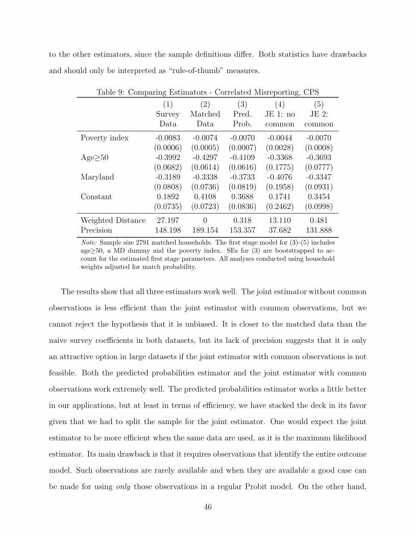
to the other estimators, since the sample definitions differ. Both statistics have drawbacks
and should only be interpreted as “rule-of-thumb” measures.
Table 9: Comparing Estimators - Correlated Misreporting, CPS
(1) (2) (3) (4) (5)Survey Matched Pred. JE 1: no JE 2:Data Data Prob. common common
Poverty index -0.0083 -0.0074 -0.0070 -0.0044 -0.0070(0.0006) (0.0005) (0.0007) (0.0028) (0.0008)
Age≥50 -0.3992 -0.4297 -0.4109 -0.3368 -0.3693(0.0682) (0.0614) (0.0616) (0.1775) (0.0777)
Maryland -0.3189 -0.3338 -0.3733 -0.4076 -0.3347(0.0808) (0.0736) (0.0819) (0.1958) (0.0931)
Constant 0.1892 0.4108 0.3688 0.1741 0.3454(0.0735) (0.0723) (0.0836) (0.2462) (0.0998)
Weighted Distance 27.197 0 0.318 13.110 0.481Precision 148.198 189.154 153.357 37.682 131.888
Note: Sample size 2791 matched households. The first stage model for (3)-(5) includesage≥50, a MD dummy and the poverty index. SEs for (3) are bootstrapped to ac-count for the estimated first stage parameters. All analyses conducted using householdweights adjusted for match probability.
The results show that all three estimators work well. The joint estimator without common
observations is less efficient than the joint estimator with common observations, but we
cannot reject the hypothesis that it is unbiased. It is closer to the matched data than the
naive survey coefficients in both datasets, but its lack of precision suggests that it is only
an attractive option in large datasets if the joint estimator with common observations is not
feasible. Both the predicted probabilities estimator and the joint estimator with common
observations work extremely well. The predicted probabilities estimator works a little better
in our applications, but at least in terms of efficiency, we have stacked the deck in its favor
given that we had to split the sample for the joint estimator. One would expect the joint
estimator to be more efficient when the same data are used, as it is the maximum likelihood
estimator. Its main drawback is that it requires observations that identify the entire outcome
model. Such observations are rarely available and when they are available a good case can
be made for using only those observations in a regular Probit model. On the other hand,
46

the predicted probabilities estimator only requires a consistent estimate of the parameters
of the misreporting model, which can often be obtained from other studies, as in Bollinger
and David (1997) and does not require the linked data to be available.
An important concern for these estimators besides bias and efficiency is their robust-
ness to misspecification. One will usually not be able to assess whether one has actually
improved things by using a correction for misreporting. If there is no validation data, one
can see whether estimates change, but usually not know whether they change for better or
for worse. The results from applying the estimators that are only consistent if misreport-
ing is conditionally random when this assumption fails indicate that the latter is certainly
possible. Thus, it is important to know how robust the corrections are, i.e. how likely it
is that their results are far off due to some minor misspecification. Informal evidence from
using subsamples (such as one of the two states) to identify the misreporting model suggest
that neither of the estimators is particularly sensitive to minor misspecification, but the
joint estimator with common observations is more robust than the predicted probabilities
estimator. In the MC study where misreporting is conditionally random, both joint estima-
tors fared a lot better than the predicted probabilities estimator, which suggests that the
predicted probabilities estimator is sensitive to the inclusion of irrelevant variables in the
first stage. One can often avoid such misspecification by doing rigorous specification tests
on the misreporting model, which consequently is more important when using the predicted
probabilities estimator. Joint specification tests of the misreporting and the outcome model
can be constructed by testing whether the bias that is implied by the misreporting model
and the bias formulas in section 3 is equal to the difference between the coefficients from the
naive and the corrected model. It is often simple to conduct such tests by simulation as in
Bernal, Mittag and Qureshi (2012).
Overall, the main conclusions from our comparison of estimators are that one should
not assume no correlation if one does not have convincing arguments for it. If feasible, one
should use the joint estimator with common observations but if it is not feasible the predicted
47

probabilities estimator is an attractive alternative. As the main downside of the predicted
probabilities estimator is its greater sensitivity to the misreporting model, its specification
should be tested. If possible, one could additionally estimate the joint estimator without
common observations to see whether the two are consistent as a robustness check.
Many of the questions posed above are related to the value of additional information: the
HAS-Probit only depends on survey data, but improves when incorporating external infor-
mation on the conditional probabilities of misreporting. More information on misreporting
allows relaxing the assumption that it is conditionally random, which is important in order
to avoid the potentially large bias from falsely assuming it. Finally, the comparison of the
predicted probabilities estimator and the two joint estimators is informative about the value
of having the data from which the misreporting model is estimated instead of the estimated
parameters and the value of observations that directly identify the outcome model. The key
advantage of additional information in our application is that it greatly improved the robust-
ness of the estimates to misspecification, but provided smaller advantages if the model was
correctly specified. Thus, incorporating additional information appears to be more valuable
in cases where the assumptions of the model are not certain or untestable. As the estimator
that fixes α0 at 0 shows, such information may improve estimates even if it is slightly inac-
curate. Put the other way around, this means that a valid model can be a good substitute
for good data. However, several of our results show that a bad model of misreporting can
make things worse than ignoring the problem altogether.
The value of information becomes very concrete when considering validation studies: The
results above show that the information obtained from validation studies can improve survey
based estimates a lot, but validation studies are costly. This raises the question how much
one loses from correcting estimates based on validation data from previous years, a subset
of the population or even a different survey. Nothing is lost if the misreporting models
are the same in the two datasets, but if they are slightly different the loss depends on the
robustness discussed above. We examine this issue by estimating the misreporting model on
48

several subsets of our data and using it to correct outcome models based on other, disjoint
subsets: We correct estimates of food stamp take-up in the ACS using the misreporting we
observe in the CPS and vice versa to see how extrapolating from a different survey works.
For the ACS, we also use the households from IL as the validation sample and see how well
it corrects food stamp take up in MD to examine whether one could still correct estimates if
validation data are only available for some states. The misreporting models are statistically
different, but qualitatively similar in all cases, so one may be tempted to use them even
though estimates will not be unbiased. The results are consistent with our previous findings:
The joint estimator with common observations performs best both in terms of bias and
efficiency. The joint estimator without common observations still suffers from a lack of
precision. The predicted probabilities estimator does well, but contrary to the previous case
it does worse than the joint estimator with common observations. The advantage of the joint
estimator with common observations seems to increase with the degree of misspecification
in the misreporting model. All estimators do better than the naive survey estimates, so
if similar data have been validated or parameter estimates from similar data are available,
using them to correct the survey coefficients may be worth trying.
5.3 Tests for Misclassification
It should be evident from the evaluation of the estimators above that an important part
of correcting misreporting is to choose an appropriate estimator. Survey estimates can be
severely biased if misreporting is ignored, but the corrections can make things worse if invalid
simplifying assumptions are made, so it is important to know whether there is misreporting
in the data and whether it is related to the covariates. This section introduces two tests for
the presence of misreporting: one for the presence of misreporting based on the HAS-Probit
and a second one based on additional information that can also be used to test whether
misreporting is correlated with the covariates.
The first test uses the fact that the likelihood function of the HAS-Probit is an uncon-
49
strained version of the regular Probit likelihood, which restricts α0 and α1 to 0. If there is
no misreporting, the HAS-Probit will still be consistent and the probability limit of both
alphas is zero. Thus, a standard test (e.g. an LR- or χ2-Test) that α0 and α1 are jointly
zero is a consistent test of the hypothesis that there is no misreporting. If misreporting is
conditionally random, the model is correctly specified, so the test has positive power and
can be conducted using the usual variance estimator. To use it as a test against misreport-
ing in the general case that allows misreporting to be related to X, one needs to use the
variance estimator for misspecified maximum likelihood models proposed by White (1982).
While the test remains consistent in the general case, it does not always have positive power.
Consequently, if the test rejects the hypothesis that there is no misreporting, it is always
valid evidence of misreporting (or a misspecified model), but in rather special conditions, the
probability limit of the αs can be 0 despite misreporting. One should check these conditions
before concluding that there is no misreporting from the fact that the estimates of the alphas
are not different from zero.
A second test can be conducted if the data contain cells formed by observables for which
Pr(y = 1) is known. The most likely case is that one knows that it is 0 or 1 for some
cells (e.g. the probability of receiving food stamps is 0 for high income families), which
makes the test very simple: If there are observations in any of these cells for which the
value of yi has probability 0, one can reject the hypothesis that there is no misreporting in
the data. The extension to the case where it is known that Pr(y = 1) = pc in cell c for
c = 1, ..., C is straightforward. Let P = (p1, ..., pc) be the vector of known cell probabilities
and P = (p1, ..., pC) be the vector of observed cell probabilities where pc =∑
i∈c yi/nc
and nc is the number of observations in cell c. Under the null hypothesis that there is
no misreporting, P is a consistent estimator for P , so a test whether P = P is a test for
misreporting. This test can easily be implemented by regressing the observations for which
the cell probabilities are known on cell dummies and performing any of the standard tests
(e.g. an F-test) that the coefficients on the cell dummies are equal to P . The test can be
50

extended to a test of the hypothesis that misreporting is conditionally random, because P ,
α0 and α1 imply a vector of observed probabilities P (α0, α1) = α0 + (1− α0 − α1)P . A test
against known probabilities of misreporting can be conducted by using P (α0, α1) instead of
P in the test described above. A general test whether any constant conditional probabilities
are consistent with the observed data can be done by minimizing the p-value of the test
with respect to (α0, α1). The simplest way to do this is to compute the minimum distance
estimator of (α0, α1) based on the cells with known probabilities, i.e.
(αMD0 , αMD
1 ) = argminα0,α1
C∑c=1
[pc − (α0 + (1− α0 − α1)pc)]2
and test whether P = P (αMD0 , αMD
1 ). If the cell probabilities are known to be 0 or 1, the
test reduces to a test whether the means of yi are equal for all cells with Pr(y = 1) = 0 and
for all cells with Pr(y = 1) = 1.
An advantage of the second test is that its implementation is simple and it is easy to
determine the alternative hypotheses against which it has no power. It also extends easily
to a test whether misreporting is conditionally random. While the HAS-Probit can be used
to test this (either via a specification test such as the score or information matrix test or
by running it on different subsamples and testing whether the αs are equal), it is easier and
more intuitive with the second test. On the other hand, the test based on the HAS-Probit
does not require external information, so it is always feasible and does not depend on the
validity of that information. Further, the second test only uses information about certain
cells, so it really only tests for the presence of misreporting in these cells, which means that
it probably has lower power. If both tests are possible, they can be combined to exploit the
advantages of both.
51

6 Conclusion
We have derived analytic results for the bias due to misclassification in the linear probability
and the Probit model and have shown that it can be substantial and that our results are useful
to assess the bias in common applications. We have lined out conditions under which certain
features of the true parameters are robust to misclassification, so that some inference can still
be based on the biased coefficients without any additional assumptions or information. Some
of the estimators that take misclassification into account have been found to perform well,
but which ones work well depends on the nature of the misclassification, so we have proposed
two tests for the presence of misclassification and whether it is related to the covariates. The
evaluation of the estimators suggests that the true parameters can be estimated from noisy
data if the misclassification model is well-specified. The estimators are not too sensitive to
small misspecifications, but may perform worse than the naive model if key assumptions
such as independence of the covariates are erroneously made. Additional information on the
nature of the misclassification process not only helps to avoid invalid assumptions, but can
also help to increase the robustness of the estimators by placing additional restrictions on
the model.
The last points underline the importance of future research on the extent and charac-
teristics of misclassification in economic data. Knowing more about misclassification in the
data would allow us to make better use of the formulas above to assess the bias in the naive
coefficients and would enable us to analyze whether the conclusions we draw from them are
affected by misclassification. We have found some regularities such as that signs tend to be
unaffected and coefficients attenuated that do not necessarily hold in general. Further knowl-
edge about misclassification in the data may confirm these regularities and thereby increase
our confidence in inference from contaminated data. Information about misclassification can
also make one of the estimators that are consistent in the presence of misreporting feasible
or justify the restrictive assumptions that allow the use of one of the simpler estimators.
52

Appendix A: Proof of Equation 6
Equation (6) gives the expectation of the coefficients in the linear probability model when
the conditional probabilities of misreporting are constants as in Hausman, Abrevaya and
Scott-Morton (1998), i.e. when
Pr(yi = 1|yTi = 0) = α0i = α0
Pr(yi = 0|yTi = 1) = α1i = α1
∀i
By the assumptions of the linear probability model Pr(yTi = 1|X) = xβLPM and Pr(yTi =
0|X) = 1 − xβLPM , so that the probability mass function of the measurement error, U ,
conditional on X is
Pr(U = ui|X = xi) =
Pr(yi = 1|yTi = 0) · Pr(yTi = 0|X) = α0(1− xiβ
LPM) if ui = 1
1− α0 + (α0 − α1)xiβLPM if ui = 0
Pr(yi = 0|yTi = 1) · Pr(yTi = 1|X) = α1xiβLPM if ui = −1
where the probability for ui = 0 follows immediately from the fact that the probabilities
have to sum to 1. Consequently, the conditional expectation of the measurement error is
E(ui|X = xi) = 1 · [α0(1− xiβLPM)] + 0 · [1− α0 + (α0 − α1)xiβ
LPM ]− 1 · [α1xiβLPM ]
= α0 − (α0 + α1)xiβLPM
Assuming that X is non-stochastic12, this implies that the bias, E(δ), is
E(δ) = E(X ′X)−1(X ′u)
= (X ′X)−1E(X ′u)
= (X ′X)−1∑i
xiE(ui|xi)
12The extension to stochastic X follows from the law of iterated expectation.
53

= (X ′X)−1∑i
xi(α0 − (α0 + α1)xiβLPM)
= (X ′X)−1∑i
xiα0 − (α0 + α1)(X′X)−1
∑i
xixiβLPM
= (X ′X)−1X ′α0 − (α0 + α1)(X′X)−1(X ′X)βLPM
= (α0, 0, . . . , 0)′ − (α0 + α1)β
LPM
The first term is the coefficient vector from a regression of a constant, α0, on X, so the
intercept will be equal to α0 and all other coefficients will be zero. The expectation of the
biased coefficient vector is E( ˆβLPM) = βLPM + E(δ). Consequently, the expectation of the
(biased) intercept is
E( ˆβLPM0 ) = α0 + (1− α0 − α1)β
LPM0
and the expectation of the (biased) slope parameters is
E( ˆβLPM1...k ) = (1− α0 − α1)β
LPM1...k
54

Appendix B: Likelihood of the Joint Estimator
As discussed in section 5.1, the sample used for estimation can be divided into three disjoint
subsamples. The first subsample, S1 contains observations that are in the validation data, but
not in the data used to identify the outcome model and thus contains (yi, yTi , x
FPi , xFN
i ). This
sample identifies the parameters of the misreporting equations, but not the outcome equation.
The second subsample, S2, contains all observations that have been validated and include
all variables in the outcome model, so that it contains (yi, yTi , xi, x
FPi , xFN
i ). This sample
identifies all parameters. The third subsample, S3, contains the observations used to estimate
the outcome model that have not been validated. Thus, it contains (yi, xi, xFPi , xFN
i ), which
by itself identifies none of the parameters. Frequently, one of the first two samples will
be empty. For the joint estimator with common observations, S1 is empty; For the joint
estimator with common observations, S2 is empty as in Bollinger and David (1997).
Since the subsamples are disjoint and independent, the log-likelihood of the entire sample
is the sum of the three log-likelihoods of the subsamples:
ℓ(y, yT , x, xFP , xFN ; β, γFP , γFN) =∑iϵS1
ℓS1i (yi, y
Ti , x
FPi , xFN
i ; γFP , γFN)+
∑iϵS2
ℓS2i (yi, y
Ti , xi, x
FPi , xFN
i ; β, γFP , γFN)+ (24)
∑iϵS3
ℓS3i (yi, xi, x
FPi , xFN
i ; β, γFP , γFN)
Equation (23) and the assumption that the error terms in all three equations are indepen-
dent draws from standard normal distributions imply the following (conditional) probabilities
Pr(yi|yTi = 0, xFPi ) =
[Φ(xFP
i γFP )]yi
+[1− Φ(xFP
i γFP )]1−yi
Pr(yi|yTi = 1, xFNi ) =
[Φ(xFN
i γFN)]yi
+[1− Φ(xFN
i γFN)]1−yi
(25)
Pr(yTi |xi) = Φ(xiβ)yTi + [1− Φ(xiβ)]
1−yTi
55

The first probability is the likelihood contribution of an observation in S1 with yTi = 0,
while the second probability is the liklihood contribution of an observation in S1 with yTi = 1.
Consequently, the likelihood contribution of an observation from S1 is
ℓS1i (yi, y
Ti , x
FPi , xFN
i ; γFP , γFN) =(1− yTi )[yi lnΦ(xFPi γFP ) + (1− yi) lnΦ(−xFP
i γFP )]+
yTi [(1− yi) lnΦ(xFNi γFN) + yi lnΦ(−xFN
i γFN)]
This is the sum of the likelihoods of probit models for false positives and false negatives.
The likelihood contribution of an observation in sample S2 is the probability of the
observed combination of yi and yTi , which is
Pr(yi, yTi |xi, x
FPi , xFN
i ) =
{Pr(yi|yTi = 0, xFP
i ) Pr(yTi = 0|xi) if yTi = 0
Pr(yi|yTi = 1, xFNi ) Pr(yTi = 1|xi) if yTi = 1
Using the probabilities from (25) yields the likelihood contribution of an observation from
sample S2:
ℓS2i (yi, y
Ti , x, x
FPi , xFN
i ; β, γFP , γFN) =
(1− yTi ) ln([yiΦ(x
FPi γFP ) + (1− yi)Φ(−xFP
i γFP )]Φ(−xiβ))+
yTi ln([(1− yi)Φ(x
FNi γFN) + yiΦ(−xFN
i γFN)]Φ(xiβ))
Equation (25) defines the probabilities of false positives as α0i = Φ(xFPi γFP ) and of false
negatives as α1i = Φ(xFNi γFN). Using these probabilities of misreporting in equation (17)
yields the contribution of an observation from S3:
ℓS3i (yi, xi, x
FPi , xFN
i ; β, γFP , γFN) =
yi ln[Φ(xFPi γFP ) + (1− Φ(xFP
i γFP )− Φ(xFNi γFN))Φ(xiβ)]+
(1− yi) ln[1− Φ(xFPi γFP )− (1− Φ(xFP
i γFP )− Φ(xFNi γFN))Φ(xiβ)]
Using the three likelihood contributions ℓS1i , ℓS2
i and ℓS3i in equation (24) and maximizing
56

it with respect to (β, γFP , γFN) yields consistent estimates of the three parameter vectors by
the standard arguments for the consistency of maximum likelihood. Standard errors of all
parameters can be obtained as usual. The joint estimator with common observations used
above assumes that S1 is empty, so the log-likelihood reduces to
ℓJE1(y, yT , x, xFP , xFN ; β, γFP , γFN) =∑iϵS2
[(1− yTi ) ln
([yiΦ(x
FPi γFP ) + (1− yi)Φ(−xFP
i γFP )]Φ(−xiβ))+
yTi ln([(1− yi)Φ(x
FNi γFN) + yiΦ(−xFN
i γFN)]Φ(xiβ)) ]
+∑iϵS3
[yi ln[Φ(x
FPi γFP ) + (1− Φ(xFP
i γFP )− Φ(xFNi γFN))Φ(xiβ)]+
(1− yi) ln[1− Φ(xFPi γFP )− (1− Φ(xFP
i γFP )− Φ(xFNi γFN))Φ(xiβ)]
]The second joint estimator we use above, the joint estimator without common observa-
tions, assumes that S2 is empty, so the log-likelihood reduces to
ℓJE2(y, yT , x, xFP , xFN ; β, γFP , γFN) =∑iϵS1
[(1− yTi )[yi lnΦ(x
FPi γFP ) + (1− yi) lnΦ(−xFP
i γFP )]+
yTi [(1− yi) lnΦ(xFNi γFN) + yi lnΦ(−xFN
i γFN)]]+∑
iϵS3
[yi ln[Φ(x
FPi γFP ) + (1− Φ(xFP
i γFP )− Φ(xFNi γFN))Φ(xiβ)]+
(1− yi) ln[1− Φ(xFPi γFP )− (1− Φ(xFP
i γFP )− Φ(xFNi γFN))Φ(xiβ)]
]Note that the likelihood contribution of S2 can be re-written as the sum of the likeli-
hood contribution if the observation were in sample S1 and the likelihood contribution to a
standard probit likelihood:
ℓS2i (yi, y
Ti , x, x
FPi , xFN
i ; β, γFP , γFN) =ℓS1i (yi, y
Ti , x
FPi , xFN
i ; γFP , γFN)+
yTi lnΦ(xiβ) + (1− yTi ) lnΦ(−xiβ)
57

This can be used to re-write the log-likelihood function as
ℓ(y, yT , x, xFP , xFN ; β, γFP , γFN) =∑
iϵS1∪S2
ℓS1i (yi, y
Ti , x
FPi , xFN
i ; γFP , γFN)+
∑iϵS2
ℓPi (yTi , xi; β) +
∑iϵS3
ℓS3i (yi, xi, x
FPi , xFN
i ; β, γFP , γFN)
where ℓP is the log-likelihood function of a standard probit model. This shows more clearly
which observations contribute to the identification of the parameters. In particular, it shows
the value of observations in S2, because in addition to the likelihood contribution of an obser-
vation in S1, they add a term that directly identifies the parameters of the outcome model,
β. It also shows that observations in S3 contribute to the identification of the parameters of
false positives and false negatives even though these observations only contain information
on the observed dependent variable.
58

References
Abrevaya, Jason, and Jerry A. Hausman. 1999. “Semiparametric Estimation with Mis-
measured Dependent Variables: An Application to Duration Models for Unemployment
Spells.” Annales d’Economie et de Statistique, 55-56: 243–275.
Aigner, Dennis J. 1973. “Regression with a binary independent variable subject to errors
of observation.” Journal of Econometrics, 1(1): 49–59.
Bernal, Pedro, Nikolas Mittag, and Javaeria Qureshi. 2012. “Identifying the effect of
School Quality on Student Achievement using Multiple Proxies.” Unpublished Manuscript.
Bitler, Marianne P., Janet Currie, and John K. Scholz. 2003. “WIC Eligibility and
Participation.” The Journal of Human Resources, 38: 1139–1179.
Black, Dan A., Seth Sanders, and Lowell Taylor. 2003. “Measurement of Higher Edu-
cation in the Census and Current Population Survey.” Journal of the American Statistical
Association, 98: 545–554.
Bollinger, Christopher R. 1996. “Bounding mean regressions when a binary regressor is
mismeasured.” Journal of Econometrics, 73(2): 387–399.
Bollinger, Christopher R., and Martin H. David. 1997. “Modeling Discrete Choice
With Response Error: Food Stamp Participation.” Journal of the American Statistical
Association, 92(439): 827–835.
Bollinger, Christopher R., and Martin H. David. 2001. “Estimation with Response
Error and Nonresponse: Food-Stamp Participation in the SIPP.” Journal of Business &
Economic Statistics, 19(2): 129–41.
Bound, John, Charles Brown, and Nancy Mathiowetz. 2001. “Measurement error in
survey data.” In Handbook of Econometrics. Vol. 5, , ed. James J. Heckman and Edward
Leamer, Chapter 59, 3705–3843. Amsterdam:Elsevier.
59
Bound, John, Charles Brown, Greg J. Duncan, and Willard L. Rodgers. 1994.
“Evidence on the Validity of Cross-Sectional and Longitudinal Labor Market Data.” Jour-
nal of Labor Economics, 12(3): 345–368.
Call, Kathleen Thiede, Gestur Davidson, Michael Davern, and Rebecca Nyman.
2008. “Medicaid undercount and bias to estimates of uninsurance: new estimates and
existing evidence.” Health Services Research, 43(3): 901–914.
Cameron, Stephen V., and James J. Heckman. 2001. “The Dynamics of Educa-
tional Attainment for Black, Hispanic, and White Males.” Journal of Political Economy,
109(3): 455–499.
Carroll, Raymond J., David Ruppert, Leonard A. Stefanski, and Ciprian M.
Crainiceanu. 2006. Measurement Error in Nonlinear Models: A Modern Perspective.
Monographs on Statistics and Applied Probability. 2nd ed., Boca Raton:Chapman &
Hall/CRC.
Collier, Paul, and Anke Hoeffler. 1998. “On Economic Causes of Civil War.” Oxford
Economic Papers, 50(4): 563–73.
Davern, Michael, Jacob A. Klerman, Jeanette Ziegenfuss, Victoria Lynch, and
George Greenberg. 2009a. “A partially corrected estimate of medicaid enrollment and
uninsurance: Results from an imputational model developed off linked survey and admin-
istrative data.” Journal of Economic & Social Measurement, 34(4): 219–240.
Davern, Michael, Jacob Alex Klerman, David K Baugh, Kathleen Thiede Call,
and George D Greenberg. 2009b. “An examination of the Medicaid undercount in
the current population survey: preliminary results from record linking.” Health Services
Research, 44(3): 965–987.
Eckstein, Zvi, and Kenneth I. Wolpin. 1999. “Why Youths Drop out of High School:
The Impact of Preferences, Opportunities, and Abilities.” Econometrica, 67(6): 1295–1339.
60
Estrella, Arturo, and Frederic S. Mishkin. 1998. “Predicting U.S. Recessions: Financial
Variables as Leading Indicators.” Review of Economics and Statistics, 80(1): 45–61.
Fearon, James D., and David D. Laitin. 2003. “Ethnicity, insurgency, and civil war.”
American Political Science Review, 97(01): 75–90.
Greene, William H. 2003. Econometric Analysis. . 5. ed., Upper Saddle River, NJ:Prentice
Hall.
Haider, Steven J., Alison Jacknowitz, and Robert F. Schoeni. 2003. “Food Stamps
and the Elderly: Why Is Participation so Low?” The Journal of Human Resources,
38: 1080–1111.
Han, Aaron K. 1987. “Non-parametric analysis of a generalized regression model : The
maximum rank correlation estimator.” Journal of Econometrics, 35(2-3): 303–316.
Hausman, Jerry A. 1978. “Specification Tests in Econometrics.” Econometrica,
46(6): 1251–1271.
Hausman, Jerry A., Jason Abrevaya, and Fiona M. Scott-Morton. 1998. “Misclassi-
fication of the dependent variable in a discrete-response setting.” Journal of Econometrics,
87(2): 239–269.
Horowitz, Joel L. 1992. “A Smoothed Maximum Score Estimator for the Binary Response
Model.” Econometrica, 60(3): 505–31.
Hsiao, Cheng, and Bao-Hong Sun. 1999. “Modeling survey response bias - with an
analysis of the demand for an advanced electronic device.” Journal of Econometrics, 89(1-
2): 15–39.
Ichimura, Hidehiko. 1993. “Semiparametric least squares (SLS) and weighted SLS esti-
mation of single-index models.” Journal of Econometrics, 58(1-2): 71–120.
61

Imbens, Guido W., and Tony Lancaster. 1994. “Combining Micro and Macro Data in
Microeconometric Models.” The Review of Economic Studies, 61(4): 655–680.
Lancaster, Tony, and Guido Imbens. 1996. “Case-control studies with contaminated
controls.” Journal of Econometrics, 71(1-2): 145–160.
Levitt, Steven D. 1998. “Juvenile Crime and Punishment.” Journal of Political Economy,
106(6): 1156–1185.
Lochner, Lance, and Enrico Moretti. 2004. “The Effect of Education on Crime: Evi-
dence from Prison Inmates, Arrests, and Self-Reports.” The American Economic Review,
94(1): 155–189.
Marquis, Kent H., and Jeffrey C. Moore. 1990. “Measurement Errors in SIPP Program
Reports.” In Proceedings of the 1990 Annual Research Conference. 721–745. Washington,
D.C.:U.S. Bureau of the Census.
Meyer, Bruce D., Wallace K. C. Mok, and James X. Sullivan. 2009. “The Under-
Reporting of Transfers in Household Surveys: Its Nature and Consequences.” Harris School
of Public Policy Studies, University of Chicago Working Papers 0903.
Meyer, Bruce, Robert Goerge, and Nikolas Mittag. 2013. “Errors in Survey Reporting
and Imputation and Their Effects on Estimates of Food Stamp Program Participation.”
Unpublished Manuscript.
Newey, Whitney K. 1985. “Maximum Likelihood Specification Testing and Conditional
Moment Tests.” Econometrica, 53(5): 1047–1070.
Poterba, James M., and Lawrence H. Summers. 1995. “Unemployment Benefits and
Labor Market Transitions: A Multinomial Logit Model with Errors in Classification.” The
Review of Economics and Statistics, 77(2): 207–16.
62
Ruud, Paul A. 1983. “Sufficient Conditions for the Consistency of Maximum Likelihood
Estimation Despite Misspecification of Distribution in Multinomial Discrete Choice Mod-
els.” Econometrica, 51(1): 225–228.
Ruud, Paul A. 1986. “Consistent estimation of limited dependent variable models despite
misspecification of distribution.” Journal of Econometrics, 32(1): 157–187.
White, Halbert. 1982. “Maximum Likelihood Estimation of Misspecified Models.” Econo-
metrica, 50(1): 1–25.
Yatchew, Adonis, and Zvi Griliches. 1984. “Specification Error in Probit Models.”
Institute for Policy Analysis, University of Toronto Working Papers 8429.
Yatchew, Adonis, and Zvi Griliches. 1985. “Specification Error in Probit Models.” The
Review of Economics and Statistics, 67(1): 134–139.
63