Mining Periodic Patterns with Gap Requirement

from Sequences ∗

Minghua Zhang Ben Kao David W. Cheung Kevin Y. Yip

Department of Computer Science,The University of Hong Kong, Hong Kong.{mhzhang, kao, dcheung, ylyip}@cs.hku.hk

Abstract

We study a problem of mining frequently occurring periodic pat-terns with a gap requirement from sequences. Given a character se-quence S of length L and a pattern P of length l, we consider P a fre-quently occurring pattern in S if the probability of observing P given arandomly picked length-l subsequence of S exceeds a certain threshold.In many applications, particularly those related to bioinformatics, in-teresting patterns are periodic with a gap requirement. That is to say,the characters in P should match subsequences of S in such a way thatthe matching characters in S are separated by gaps of more or less thesame size. We show the complexity of the mining problem and dis-cuss why traditional mining algorithms are computationally infeasible.We propose practical algorithms for solving the problem, and studytheir characteristics. We also present a case study in which we applyour algorithms on some DNA sequences. We discuss some interestingpatterns obtained from the case study.

1 Introduction

The completion of whole-genome sequencing of various organisms facilitatesthe detection of many kinds of interesting patterns in DNA and proteinsequences. It is now well known that the genomes of most plants and animalscontain large quantity of repetitive DNA fragments. For instance, it isestimated that one third of the human genome is composed of families of

∗This research is supported by Hong Kong Research Grants Council grant HKU7040/02E.

1

reiterated sequences [9]. The genomes are thus far from pieces of randomstrings, and it is widely believed that a substantial amount of currentlyunknown information can be extracted from the sequences.

A large number of studies on genome sequence mining are related to theidentification of periodic patterns. This is largely due to the abundance andvariety of periodic patterns existing in the genomes. From the short threebase pair (bp) periodicity in protein coding DNA [5] and the medium-lengthrepetitive motifs found in some proteins [4] to the mosiac of very long DNAsegments in the genome of warm-blooded vertebrates [3], periodic patterns ofdifferent lengths and types are found at both genomic and proteomic levels.Some of the patterns have been identified as having significant biologicaland medical values. For example, some repeats have been shown to affectbacterial virulence to human [19], while the excessive expansions of someVariable Number of Tandem Repeats (VNTRs) are the suspected cause ofsome nervous system diseases [14]. Efficient algorithms for searching periodicpatterns from long sequences are therefore of growing importance.

Computationally, a DNA or protein sequence is treated as a long stringof characters with a finite alphabet. The alphabet used in modeling a DNAsequence is usually the four-character set {A,C,G, T} representing the fournitrogenous bases Adenine, Cytosine, Guanine and Thymine. For proteinsequences, the commonly used alphabet is the set of twenty amino acids.

Two types of periodic patterns have received much attentions: tandemrepeats and base pair oscillations. Given a (DNA or protein) sequences = s1s2s3 · · · sL of length L and an integer p (the period), a tandem repeatis a subsequence sisi+1si+2 · · · si+2p−1 where si+j = si+p+j , for 0 ≤ j < p.The basic computational problem is to find all tandem repeats in a givensequence. There are many variations of the problem, considering issues likethe number of periods (tandem repeats vs. tandem arrays), the maximal-ity of patterns, whether errors (insertions, deletions and substitutions) areallowed and the corresponding cost functions, palindromic reverses, and ef-ficient approximate solutions. A recent survey on the works can be foundin [9]. We are particularly interested in tandem repeats that are related tothe three-dimensional structure of the sequence. For example, the proteinsequence of the molecule porcine ribonuclease inhibitor (SwissProt entryRINI PIG [2]) consists of an alternating pattern of two kinds of repeatswith lengths 29 and 28 residues [4]. The two can be combined to form arepeating unit of 57 residues, and there are 7.5 such units in the molecule.As a result, the protein has a horseshoe shape with the interior face formedby a parallel β sheet of 17 β strands and the exterior face formed by 16 α

2

helices1.It should be noted that the repeats are not error-free. For instance, a

phase shift is found in one of the repeats, which may be due to the insertionor deletion of a short sequence.

The second kind of important periodic pattern is base pair oscillations,which correspond to unexpected correlations between bases of distance p.For example, the probability of having a ‘T ’ located p bp after an ‘A’ canbe calculated as nAT (p)

L−p , where nAT (p) is the number of such occurrences inthe sequence and L − p is the number of base pairs located p bp apart. Ifbase pairs of distance p are independent, then the expected probability willbe pr(A)pr(T ), which is the product of the probabilities of occurrence of thetwo individual bases in the sequence. The difference nAT (p)

L−p − pr(A)pr(T )can be used to reflect the correlation between the two bases at a distanceof p apart [7]. It has been shown in [20, 7] that some base pairs exhibit anabnormally high correlation at a period of 10-11 base pairs and its multiplesin many kinds of organisms. It is believed that a partial reason for thephenomenon is related to the helical structure of the DNA, which has aperiod of about 10-11 base pairs in some organisms [7]. In other words, forsome base pairs, if the first one is found in a certain position, there is anabnormally high probability of finding the second one after about one helicalturn. Some interesting periodic patterns may thus be found in successivebases with similar 3D orientations.

Our study is based on the above observation. We would like to search forfrequent periodic patterns that consist of bases physically located one helicalturn after another. Symbolically, a pattern is defined as a subsequence

sisi+g1si+g1+g2 · · · si+g1+g2+···+gl−1 ,

where l is the length (number of bases) in the subsequence and gj , 1 ≤ j < lis the length of period j. Unlike previous studies, we define gj as a rangeof integers instead of a fixed integer. The reason for this setting is two-fold:1) the actual period of a helical turn is usually not an integer and 2) theactual period may vary in organisms. The introduction of a variable periodthus provides a flexible way to capture any interesting patterns hidden in asequence.

While the primary focus of our study is on the periodic patterns in DNAsequences due to its 3D structure, the techniques being developed can also beapplied to mine other kinds of sequences, in which case the variable period

1A figure of the protein can be found in Figure 1 of [4] at http://www.nslij-genetics.org/dnacorr/.

3

can be used to model the maximum allowed insertions/deletions within asingle period.

The rest of the paper is organized as follows. Section 2 mentions somerelated works. Section 3 formally defines our computational problem. InSection 4 we prove a couple of important theorems that lead to the deriva-tion of efficient algorithms for our mining problem. Section 5 presents thealgorithms. In Section 6 we analyze the algorithms’ performance. Section 7presents a case study in which we document an interesting finding obtainedby applying our algorithm to mining DNA sequences. Finally, Section 8concludes the paper.

2 Related Works

Besides the studies on tandem repeats and base-pair oscillation, there areother related works that include studies on mining patterns from biologicalsequences with certain support requirement. For example, the TEIRESIASalgorithm [15] is designed for discovering patterns that are composed of char-acters (such as {A,C, T, G}) and wild-cards (which match any characters)from biological sequences. Although wild-cards provide some flexibility inspecifying a pattern, too many unrestricted wild-cards in a pattern wouldrender the pattern uninteresting. Therefore, the authors restrict the num-ber of wild-cards that can be present in the extracted patterns. In anotherstudy [8], the Pratt algorithm is proposed for mining restricted patternsfrom a sequence database. The restrictions include the maximum numberof characters and wild-cards in a pattern.

BLAST [1] is one of the famous algorithms in the area of bioinformatics.Given a query sequence, it searches for matched sequences from a database.In essence, BLAST is a search algorithm with a query as input, while ourmodel is focused on mining unknown knowledge.

From the area of data mining, one related problem is to find frequentsequences from transactional databases. Many efficient algorithms have beenproposed for the problem [16, 22, 23, 12]. Their goal is to find patterns thatappear in at least a certain number of sequences in the database. All thealgorithms are based on the well-known Apriori property. Unfortunately,as we will see later, this property does not hold for our problem. Also, thesequence mining algorithms find patterns across sequences. On the otherhand, our model is to discover patterns within a sequence. Moreover, thecharacteristics of the biological sequences (e.g., very long sequence with veryfew different characters) makes a direct application of those sequence mining

4

algorithms inefficient.There are also some algorithms on mining frequent patterns from a sin-

gle sequence [10, 6]. In [10], the input sequence is divided into some over-lapped windows of fixed width w, and every two neighboring windows sharea common segment of length (w − 1). In [6], a sequence is divided intonon-overlapping windows. In both papers, a pattern is frequent if it appearsin at least a certain number of windows. With this definition, it is shownthat the Apriori property applies. By segmenting a sequence into windowsand counting the number of windows in which a pattern occurs greatly sim-plifies the design of the mining algorithm. The drawback is that patternsthat span multiple windows cannot be discovered, and that in some cases,a suitable window width is difficult to determine. Our model does not havethose restrictions.

Yang et al. studied asynchronous periodic patterns in time series data [21].In their model, shifts in the occurrence of patterns are permitted to filterout random noises. They also consider a range of periods instead of the pre-specified ones as used in [6], although there is still a limit on the maximumlength of a period. In their model, the Apriori property holds for patternsof the same period.

3 Problem Definition

In this section we give a formal definition of the periodic pattern miningproblem. To simplify our discussion, let us first define a number of notationsand terms.

A sequence from which we extract frequent patterns is called a subjectsequence. Let

∑be the alphabet of all possible characters that occur in

a subject sequence. For example,∑

= {A,C, G, T} for DNA sequences; forprotein sequences,

∑is the set of 20 amino acids.

A wild-card (denoted by a single dot, ‘.’) is a special symbol thatmatches any character in

∑. A gap is a sequence of wild-cards. The size

of a gap refers to the number of wild-cards in it. For example, the size of‘.....’ is 5. We use g(N) to represent a gap of size N ; we use g(N, M) torepresent a gap whose size is within the range [N, M ]. The range [N,M ] iscalled a gap requirement.

A pattern is a sequence of characters and gaps that begins and endswith characters. We define the length of a pattern P , denoted by |P |, as thenumber of characters in P . For example, if P = A..T.C, then |P | = 3. Notethat the wild-card symbols are not counted towards the pattern’s length.

5

Given a pattern P , a substring Q of P is called a sub-pattern of P if Qitself is also a pattern (i.e., Q also starts and ends with characters). If |P | ≥2, its sub-pattern containing the first |P | − 1 characters is called the prefixof P . Similarly, the sub-pattern of P that contains the last |P |−1 charactersis called the suffix of P . We use prefix(P ) and suffix(P ) to represent theprefix and suffix of P , respectively. For example, prefix(A..T.C) = A..T andsuffix(A..T.C) = T.C.

Given a subject sequence S (a pattern P ), we use S[i] (P [i]) to representthe i-th character of S (P ). For example, if S = ACGTA, then S[1] = A,S[2] = C, etc. If P = A..T.C, then P [1] = A, P [2] = T .

For our problem of mining periodic patterns from a sequence, we areinterested in patterns of the following form:

a1g(N,M)a2g(N, M) . . . al−1g(N, M)al (1)

where ai ∈∑

for 1 ≤ i ≤ l, and N , M are two user supplied numbers thatspecify the minimum and maximum gap sizes between two successive char-acters in a pattern, respectively. If the gap size requirement is understood,as a shorthand, we express a pattern P by simply specifying the charactersit contains (i.e., a1a2 . . . al). For example, if N = 8 and M = 10, the pat-tern written as ATC refers to the pattern Ag(8, 10)Tg(8, 10)C. Since themining problem is defined with specified values of N and M , in the follow-ing discussion, we use the shorthand notation for patterns, unless otherwisestated.

Given a sequence S of length L, an offset sequence of length l isa sequence of integers [c1, . . . , cl], such that 1 ≤ cj ≤ L for all j, andcj+1 − cj − 1 ∈ [N, M ] for all 1 ≤ j ≤ l − 1. Essentially, an offset sequenceis simply a sequence of positions of S that satisfies the gap requirement.

Our goal is to determine frequently occurring patterns given a subjectsequence S. Hence, we need to define the term frequency and how often apattern P occurs before we consider it frequent in S. We define frequencyof a pattern P by the probability of observing P if we randomly pick |P |positions of S (i.e., a random offset sequence) that satisfy the gap require-ment. Also, a pattern P is considered frequent, if its frequency exceedscertain user-specified threshold value, ρs.

Given a sequence S, a pattern P , and an offset sequence [c1, . . . , c|P |],we say that P matches S w.r.t. the offset sequence if S[cj ] = P [j] for all1 ≤ j ≤ |P |. We define the support of P w.r.t. S (denoted by sup(P ))as the number of distinct offset sequences with respect to which P matchesS. For example, if S = AAGCC, P = AC, and gap requirement is [2, 3],

6

then P matches S w.r.t. the offset sequence [1, 4] since S[1] = P [1] andS[4] = P [2]. Similarly, P matches S w.r.t. the offset sequences [1, 5] and[2, 5]. So sup(P ) = 3. A straightforward way to compute P ’s support isto enumerate all possible offset sequences, check the contents of S withrespect to all those offset sequences, and determine the fraction of the offsetsequences with respect to which P matches S. If the fraction exceeds therequired threshold ρs, P is frequent; otherwise P is infrequent.

To determine whether a pattern P of length l is frequent with respect toa sequence S, we need two numbers: (1) Nl, the number of offset sequencesof length l in S and (2) sup(P ). If the support ratio, sup(P )/Nl, is largerthan ρs, P is a frequent pattern.

In the following section, we derive a formula for computing Nl. In Sec-tion 5, we derive algorithms for computing all patterns P that satisfy thefrequency requirement.

4 Mathematical Analysis

In this section we derive a recurrence equation for determining the value ofNl. We also prove several important theorems that allow us to formulateefficient algorithms for solving the periodic pattern mining problem. Forreference, Table 1 shows the various symbols and their definitions we use inthis section.

We use the variable W to denote the flexibility of the gap requirement.For example, if the gap requirement is [4, 6], then the flexibility is 6−4+1 =3. That is to say, if the first character of a pattern P matches the sequence Sat a certain position, say j (i.e., P [1] = S[j]), then there are three possiblepositions of S for P [2] to match against, namely, S[j + 5], S[j + 6] andS[j + 7]. Also, the larger is the flexibility, the larger is the number of offsetsequences that satisfy the gap requirement, and so, the value of Nl will belarger.

We use minspan(l) to denote the minimum span of a length-l patternP . As an example, with a gap requirement of [3, 4], a length-3 patternspans at least 9 positions of the subject sequence. This is obtained bytaking the smallest gap of 3 positions between the first and the secondcharacters of P , and 3 positions between the second and the third. (Figure 1illustrates the concept.) Since a length-l pattern has l characters and l − 1gaps and the minimum gap size is N , the minimum span is thus equal to(l − 1)N + l. Similarly, we can determine the maximum span of a length-lpattern (denoted by maxspan(l)), which is equal to (l − 1)M + l.

7

Symbol DefinitionS A subject sequenceP A patternN The minimum gap between 2 successive

characters in a patternM The maximum gap between 2 successive

characters in a patternL Length of S; L = |S|l Length of P ; l = |P |

W Flexibility of a gap; W = M −N + 1minspan(l) The minimum span of a length-l pattern

minspan(l) = (l − 1)N + lmaxspan(l) The maximum span of a length-l pattern

maxspan(l) = (l − 1)M + ll1 The length of a longest pattern whose

maximum span is ≤ |S|l1 = bL+M

M+1 cl2 The length of a longest pattern whose

minimum span is ≤ |S|l2 = bL+N

N+1 c

Table 1: Notations

N N N

P[1]

. . .

P[3]P[2]

. . .

P[l]P[l-1]

. . .. . . . . . S:

Figure 1: Illustration of minspan

8

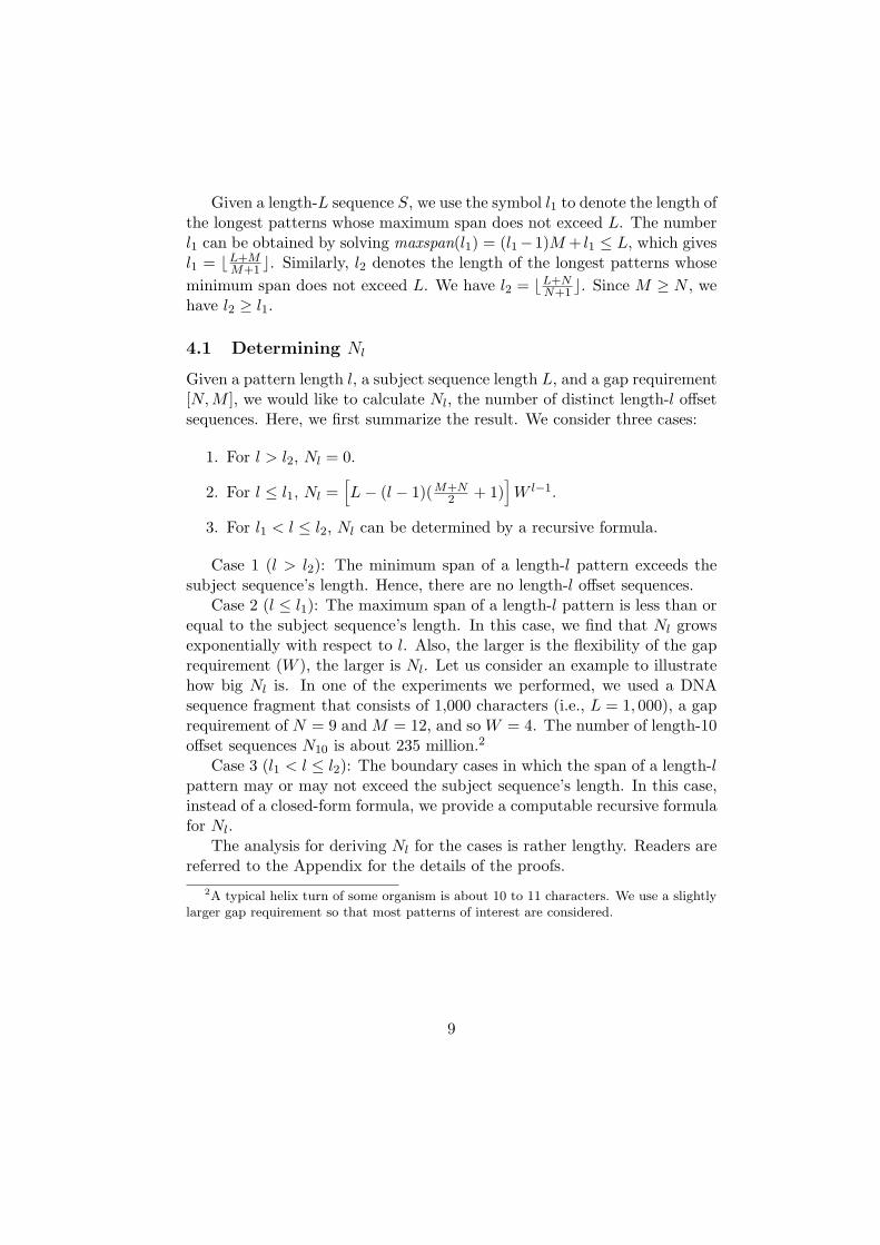
Given a length-L sequence S, we use the symbol l1 to denote the length ofthe longest patterns whose maximum span does not exceed L. The numberl1 can be obtained by solving maxspan(l1) = (l1−1)M + l1 ≤ L, which givesl1 = bL+M

M+1 c. Similarly, l2 denotes the length of the longest patterns whoseminimum span does not exceed L. We have l2 = bL+N

N+1 c. Since M ≥ N , wehave l2 ≥ l1.

4.1 Determining Nl

Given a pattern length l, a subject sequence length L, and a gap requirement[N, M ], we would like to calculate Nl, the number of distinct length-l offsetsequences. Here, we first summarize the result. We consider three cases:

1. For l > l2, Nl = 0.

2. For l ≤ l1, Nl =[L− (l − 1)(M+N

2 + 1)]W l−1.

3. For l1 < l ≤ l2, Nl can be determined by a recursive formula.

Case 1 (l > l2): The minimum span of a length-l pattern exceeds thesubject sequence’s length. Hence, there are no length-l offset sequences.

Case 2 (l ≤ l1): The maximum span of a length-l pattern is less than orequal to the subject sequence’s length. In this case, we find that Nl growsexponentially with respect to l. Also, the larger is the flexibility of the gaprequirement (W ), the larger is Nl. Let us consider an example to illustratehow big Nl is. In one of the experiments we performed, we used a DNAsequence fragment that consists of 1,000 characters (i.e., L = 1, 000), a gaprequirement of N = 9 and M = 12, and so W = 4. The number of length-10offset sequences N10 is about 235 million.2

Case 3 (l1 < l ≤ l2): The boundary cases in which the span of a length-lpattern may or may not exceed the subject sequence’s length. In this case,instead of a closed-form formula, we provide a computable recursive formulafor Nl.

The analysis for deriving Nl for the cases is rather lengthy. Readers arereferred to the Appendix for the details of the proofs.

2A typical helix turn of some organism is about 10 to 11 characters. We use a slightlylarger gap requirement so that most patterns of interest are considered.

9

. . .

. . .. . .

i+l-d-1i. . .

i-1 d-i+1

P:

Q:

Figure 2: Patterns P and Q

4.2 Determining Frequent Patterns

Like many other data mining problems, our objective is to discover frequentpatterns from data under a definition of “frequent”. A common difficultyshared by most mining problems is that the number of patterns is huge. Soa straightforward method of enumerating all possible patterns and countingtheir supports is not feasible. Traditional mining algorithms achieve effi-ciency by various pruning techniques that aim at drastically reducing thenumber of patterns that need to be checked. One very important propertythat enables effective pruning is the Apriori property, which states that “thesupport of a pattern cannot exceed the support of any of its sub-patterns.”The Apriori property is shown to hold under many data mining problemsand models. The well-known Apriori algorithm [13] is a classic examplethat uses the Apriori property. In Apriori, an itemset X cannot be fre-quent if any proper subset of X is not frequent, and in which case, X ispruned.

For our mining problem, the Apriori property, however, does not hold.As a simple example, consider the sequence S = ACTTT , the pattern P1 =AT and its sub-pattern P2 = A. If the gap requirement is [1, 3], we seethat sup(P1) = 3 (corresponding to the offset sequences {[1, 3], [1, 4], [1, 5]})while sup(P2) = 1 (corresponding to the offset sequence {[1]}). Hence, thesupport of a pattern can exceed the support of its sub-pattern.

To achieve pruning, we derive an apriori-like property. Theorems 1 and2 summarize the property.

Theorem 1 Given a length-l pattern P and a length-(l − d) sub-patternQ = P [i]P [i + 1] . . . P [i + l − d − 1] of P , where 1 ≤ i ≤ d + 1, we havesup(Q) ≥ sup(P )/W d.

Proof: Let U be the set of all length-l offset sequences with respect towhich P matches S. We have sup(P ) = |U |. We partition U into Rsubsets U1, . . . , UR such that two offset sequences A = [ca1 , . . . , cal

] andB = [cb1 , . . . , cbl

] are in the same subset Uj if and only if cak= cbk

∀i ≤ k ≤

10

i + l − d − 1. We see that each Uj corresponds to a unique offset sequencewith respect to which Q matches S. Therefore, sup(Q) ≥ R. Since theoffset sequences in a given Uj only differ in the first i − 1 offsets and thelast d− i + 1 offsets (see Figure 2), the cardinality of each Uj cannot exceedW (i−1)+(d−i+1) or W d. Hence, R, the number of subsets Uj ’s must be atleast equal to |U |/W d. Therefore,

sup(Q) ≥ R ≥ |U |/W d = sup(P )/W d.

2

Theorem 1 is an important one in that it allows us to prune a largenumber of candidate patterns from consideration. In particular, if a length-l pattern P is frequent, then by definition, we have sup(P )/Nl ≥ ρs. Now,consider a length-(l − d) sub-pattern Q of P . Theorem 1 requires that

sup(Q)Nl−d

≥ sup(P )Nl−dW d

≥ Nl

Nl−dW dρs = λl,d · ρs, (2)

where λl,d = Nl

Nl−dW d . That is, the support ratio of Q also has to attain acertain value.

One can also verify the following transitivity property of λ:

λl,d1+d2 = λl,d1 · λl−d1,d2 ∀0 ≤ d1 ≤ l and ∀0 ≤ d1 + d2 ≤ l. (3)

As an example, if l ≤ l1, then by Equation 2 and the value of Nl stated inSection 4.1, one can easily show that,

sup(Q)Nl−d

≥ Nl

Nl−dW dρs

=L− (l − 1)(M+N

2 + 1)L− (l − d− 1)(M+N

2 + 1)ρs. (4)

Here λl,d = Nl

Nl−dW d = L−(l−1)(M+N2

+1)

L−(l−d−1)(M+N2

+1).

For a long subject sequence (i.e., large L), a small pattern length (i.e.,small l), and a small d, the fraction λl,d is very close to 1. Therefore, if alength-l pattern P is frequent (i.e., its support ratio exceeds ρs), Theorem 1implies that any length-(l − d) sub-pattern Q of P has to have its supportratio exceed λl,d · ρs, or almost ρs as well. Hence, we obtain a property thatis very close to the apriori property. One can derive an efficient pruningalgorithm based on that observation.

11

Kr K1 K2 K3 K4 K5 K6 K7 K8

Value 2 1 2 1 0 0 0 0

Table 2: Kr of sequence ACGTCCGT

In the proof of Theorem 1, we bound the cardinality of the set Uj by W d.The bound is obtained by considering the extreme case that given an offsetsequence A = [ca1 , . . . , cai , . . . cai+l−d−1

, . . . cal] ∈ Uj , any perturbation of the

first i−1 offsets and the last d− i+1 offsets (as long as the gap requirementis still satisfied) results in another offset sequence in Uj . In other words,any such perturbation gives us an offset sequence w.r.t. which P matches S.That is to say, no matter how we change the first i−1 offsets [ca1 , . . . , cai−1 ],we observe the same sequence of characters S[ca1 ] = P [1], . . . , S[cai−1 ] =P [i− 1], and the same can be said for the last d− i + 1 offsets. The boundis obviously too loose.

We now consider a method of tightening the bound. Given a small valuem, we consider all length-(m + 1) offset sequences of the form [(r), (r +g1), . . . , (r + g1 + . . . + gm)], where each gj ∈ [N + 1,M + 1]. Let us inspectS according to those offset sequences and use Kr to denote the frequencycount of the most frequently occurring patterns observed. We repeat theexercise for each value of 1 ≤ r ≤ L. Finally, we take em = maxL

r=1 Kr.We illustrate the idea with a simple example. Suppose S = ACGTCCGT ,the gap requirement is [1, 2], and m = 2. We first calculate K1. There are4 possible length-(m + 1) (or length-3) offset sequences whose first elementis equal to 1: [1, 3, 5], [1, 3, 6], [1, 4, 6] and [1, 4, 7], and they correspond topatterns AGC, AGC, ATC, and ATG, respectively. We see that AGC isthe most frequently occurring pattern and its count is 2, so K1 = 2. ForK2, the relevant offset sequences are [2, 4, 6], [2, 4, 7], [2, 5, 7] and [2, 5, 8].Since these 4 offset sequences give 4 different patterns CTC, CTG, CCGand CCT , by definition K2 = 1. Other Kr values are calculated similarly.The results are shown in Table 2. Finally we get em = max8

r=1 Kr = 2.Semantically, for any offset r, the value em tells us how many times at

most we will see the same character sequence in S under the offset sequence[r, r + g1, . . . , r + g1 + . . . + gm] however we perturb the last m offsets inthe sequence. Essentially, we use em to replace Wm as a better bound sinceW m

em≥ 1. In the above example, W m

em= 22

2 = 2. In typical DNA sequences,we find that the ratio W m

embecomes larger as m increases.

To illustrate how the value em is used, let us re-visit Theorem 1 again

12

and consider the following example. Suppose the sub-pattern Q is takenfrom the first l − 8 characters of P (i.e., Q = P [1]P [2] . . . P [l − 8]). Ifwe follow the proof of Theorem 1 again, we see that all offset sequencesA = [ca1 , . . . , cal−8

, cal−7, . . . , cal

] in Uj only differ in the last 8 offsets. Now,suppose we have determined the value of em for the case m = 3. We knowthat, however we perturb the offsets cal−7

, cal−6, cal−5

, the maximum numberof times that we see the same character sequence (namely, P [l − 7], P [l −6] and P [l − 5]) over those three offsets is em. The same is true for theoffsets cal−4

, cal−3, cal−2

. And finally, there are at most W 2 ways for us toperturb the offsets cal−1

and cal. Hence, |Uj | ≤ e2

mW 2. This bound could bemuch smaller than W 8 Theorem 1 uses. With this discussion, the followingtheorem can be easily proved.

Theorem 2 Given a length-l pattern P and a length-(l − d) sub-patternQ = P [1] . . . P [l − d] of P such that s = bd/mc and t = d − sm, we havesup(Q) ≥ sup(P )

esmW t .

From Theorem 2, we know that if a length-l pattern P is frequent, then thelength-(l− d) sub-pattern Q of P such that Q = P [1] . . . P [l− d] must haveits support ratio lower-bounded by:

sup(Q)/Nl−d ≥ sup(P )esmW tNl−d

≥ Nl

Nl−desmW t

ρs

=W d−t

esm

· λl,d · ρs

= (Wm

em)s · λl,d · ρs

= λ′l,d · ρs, (5)

where s = bd/mc, t = d− sm, and λ′l,d = (W m

em)s · λl,d.

5 Algorithms

In the previous section we discuss why pruning is an important issue intypical mining problems. In this section we propose efficient algorithmsthat apply pruning techniques.

13

5.1 MPP

Consider Equation 4 in Section 4 again. We note that if a length-l patternP is frequent w.r.t. the support threshold ρs, then any length-(l − d) sub-pattern Q of P must have a support ratio not less than λl,d · ρs. This leadsto the following apriori-like mining algorithm. We call our algorithm MPP.

First, let us assume that the user has a rough idea about the length ofthe longest frequent patterns in the subject sequence S. Let n representssuch a length. MPP guarantees that all frequent patterns of length less thanor equal to n are returned. For the longer frequent patterns, MPP will takea best-effort approach, i.e., it will return as many of those frequent patternsas it could.

To obtain all frequent patterns of length less than or equal to n, Equa-tion 4 suggests that we obtain all length-1 patterns whose support ratios arenot less than λn,n−1 · ρs. (Other length-1 patterns would not be the con-stituents of any longer frequent patterns of interest.) From those patterns,we join them to obtain a set of length-2 candidate patterns. We examinethe subject sequence and collect all those candidate patterns whose supportratios are not less than λn,n−2 · ρs. We then join those patterns collected toform a set of length-3 candidate patterns and so on. In general, during thei-th iteration, the algorithm determines a set (denoted by L̂i) of length-ipatterns whose support ratios are not less than λn,n−i · ρs. In the (i + 1)-stiteration, patterns in L̂i are joined to form the set of candidate length-(i+1)patterns (denote by Ci+1). Patterns in Ci+1 whose support ratios are notless than λn,n−(i+1) ·ρs are collected in L̂i+1. The process repeats until either(1) MPP generates an empty candidate set, or (2) when i = n + 1.

For the second case, MPP would have returned all frequent patterns oflengths less than or equal to n. To find other longer frequent patterns, MPPreverts to a basic Apriori-like method. That is, during each iteration i > n,MPP generates candidate set Ci based on Li−1. It then checks the patternsin Ci and collects those whose support ratios are not less than ρs in Li.The process repeats until MPP generates an empty candidate set. Note thatin this candidate pattern generation process, a length-(n + k) pattern P(where k > 0) is generated (and potentially is returned by the algorithmas a frequent pattern) only if there is a length-n sub-pattern Q of P whosesupport ratio is not less than ρs. From Equation 4, however, we see thata length-(n + k) pattern can be frequent if all of its length-n sub-patternshave their support ratios reach λn+k,k · ρs, which is less than ρs. In otherwords, there could be length-(n+k) frequent patterns that are not generatedand are thus missed. As a result, MPP can only guarantee that all frequent

14

patterns of lengths less than or equal to n are discovered.There are a few issues concerning MPP as outlined above:

• First, if the user does not have a good idea about how long frequentpatterns are, he may choose an arbitrarily large n. In that case, prun-ing is not effective. For example, consider the case when MPP is deter-mining L4. The pruning condition requires that every length-4 candi-date sequence with a support ratio not less than λn,n−4 ·ρs be includedin L4. If n is very large, λn,n−4 is very small, and few candidates canbe removed.

• Second, for DNA sequences, the size of the alphabet, (e.g., |{A,C, T, G}|),is small. The number of combinations of short patterns is thus verysmall. Hence, short patterns are likely frequent. For example, in ourexperiment, we find that patterns of lengths one or two are alwaysfrequent. These patterns are thus uninteresting.

• Third, given a length-i candidate pattern P , checking its supportmight require us to examine the subject sequence S with respect toevery length-i offset sequences. As we have discussed in Section 4, thenumber of length-i offset sequences equals Ni, a very large numbereven for a moderate value of i.

For the first issue, if n > l1, MPP restricts n to l1. That is to say, MPP willonly guarantee the extraction of all frequent patterns whose lengths are lessthan or equal to l1. We remark that even without a theoretical guaranteethat all patterns longer than l1 are found, the drawback, in practice, maynot be detrimental. Incidentally, in all of the experiments we performed onDNA sequences, very long frequent patterns do not occur.

For the second issue, MPP starts with length-3 patterns, assuming thatshorter ones are uninteresting. MPP does not count their supports and savesa bit of computation.

For the third issue, MPP uses an index structure called partial index list(PIL) to avoid examining all offset sequences when counting a pattern’ssupport count.

Given a subject sequence S and a length-l pattern P , PIL(P ) is a listof (x, y) pairs where all x’s are of distinct values. If the pair (x, y) is inPIL(P ), then there are exactly y offset sequences of the form [x, c2, . . . , cl]with respect to which P matches S (i.e., P [1] = S[x], . . . , P [l] = S[cl]). Forexample, if S = AACCGTT , P = ACT , [N,M ] = [1, 2], then PIL(P ) =

15

{(1, 3), (2, 2)}. This is because P matches S with respect to three offset se-quences with the first offset equals 1 (namely, {[1, 3, 6], [1, 4, 6], [1, 4, 7]}) andtwo offset sequences with the first offset equals 2 (namely, {[2, 4, 6], [2, 4, 7]}).

There are two properties of PIL(P ):

1. Given PIL(P ), one can easily compute sup(P ), which is just the sumof all y’s in the list. Using our previous example, since PIL(P ) ={(1, 3), (2, 2)}, we have sup(P ) = 3 + 2 = 5.

2. For a pattern P , let prefix(P ) = Q1, suffix(P ) = Q2. PIL(P ) canbe computed from PIL(Q1) and PIL(Q2) using the following simpleprocedure.

1 ∀(x, y) ∈ PIL(Q1)2 t = 03 ∀(x′, y′) ∈ PIL(Q2) s.t. x′ − x− 1 ∈ [N,M ]4 t = t + y′

5 if (t > 0), insert (x, t) in PIL(P )

Figure 3 shows the algorithm MPP. The algorithm basically follows ourprevious discussion. For generating length-(i + 1) candidates, MPP considersevery pair of length-i patterns P1 and P2 in L̂i. If suffix(P1) = prefix(P2),then the candidate pattern P1[1]P2 is put into Ci+1. For example, P1 = ACGand P2 = CGT generate ACGT . MPP also calculates the PIL list of thecandidate using PIL(P1) and PIL(P2). The PIL list of the candidate patternallows us to determine its support count and therefore whether the candidateshould be added to the set L̂i+1 or not. Finally, all patterns in all L̂i’s withsupport ratios not less than ρs are returned to the user.

5.2 MPPm

The efficiency of MPP relies on how effective pruning is. In this subsectionwe discuss how MPP can be refined to improve its pruning effectiveness andthus to achieve better efficiency.

Recall that given a value of n (the length of the longest frequent patternsthe user is interested in obtaining), a candidate length-i pattern Q in theset Ci is pruned if its support ratio is less than λn,n−i · ρs. So, the largerthe value λn,n−i is, the more effective is the pruning. By the definition of λ,that implies a small n − i, or equivalently, a small n and a large i. Whilewe don’t have many choices for i (the algorithm always starts with mininglength-3 patterns, so i starts at 3), the above argument indicates that a

16

1 Algorithm MPP(S, ρs, N , M , n)2 calculate W, l1, l23 if n > l1, n = l14 for i=3 to n5 calculate Ni, λn,n−i

6 for i = n + 1 to l27 calculate Ni, and set λn,n−i = 18 C3 = the set of all length-3 patterns9 scan S to compute the PILs of all patterns in C3

10 for each pattern P in C3

11 get sup(P ) from PIL(P )12 if sup(P ) ≥ ρsN3, put P into L3

13 if sup(P ) ≥ λn,n−3ρsN3, put P into L̂3

14 i := 315 while (L̂i 6= ∅)16 Ci+1 := Gen(L̂i)17 ∀P ∈ Ci+1

18 compute PIL(P ) to get sup(P )19 if sup(P ) ≥ ρsNi+1, put P into Li+1

20 if sup(P ) ≥ λn,n−(i+1)ρsNi+1, put P into L̂i+1

21 i := i + 122 Return L3 ∪ L4 ∪ . . . ∪ Li−1

Figure 3: Algorithm MPP

17

reasonably small value of n can potentially speed up the algorithm. As anexample, in our experiment, we use a DNA fragment of 1,000 characters,a gap requirement of [9,12], and a support threshold ρs = 0.003%, thelongest pattern mined has a length of 13. If the user has a good idea of howlong frequent patterns are, and picks n = 13 as the algorithm’s input, ourexperiment shows that MPP could achieve good pruning and is efficient. Thequestion is “what if the user does not know what n to pick?” We will comeback to this question shortly.

In the derivation of Theorem 2, we discussed how to derive a tighterbound that leads to a more effective pruning strategy. Without repeatingthe details, the approach is to pick a small number m and analyze the subjectsequence to obtain a number em. From Theorem 2 and Equation 5, we knowthat if there is a length-k frequent pattern P , then the sub-pattern Q of Pthat consists of the first k − d characters (i.e., Q = P [1] . . . P [k − d]) musthave its support ratio not less than λ′k,d · ρs, where λ′k,d = (W m

em)s · λk,d,

s = bd/mc.Now, let us consider the “pick-the-n” problem again. If the user does not

have a good idea of n, our approach is to find a reasonable value automati-cally. The idea is to count the supports of all length-3 patterns. Then, forevery value of 3 < k ≤ l1, we check and see if there is any length-3 patternQ whose support is not less than λ′k,k−3 ·N3 ·ρs. If no such Q exists, then byTheorem 2, we know that there are no length-k frequent patterns. Finally,the value of n is taken as the largest k such that length-k frequent patternsmay exist. We thus modify MPP with the above procedure of automaticallydetermining n applied. We call the modified algorithm MPPm.

6 Experiment Results and Analysis

To analyze the performance of the mining algorithms, we perform an exten-sive experimental study. This section shows some representative results anddiscusses some interesting properties of the algorithms.

The data used in the experiments is the Homo Sapiens (human) DNAsequence AX829174 downloaded from the National Center for BiotechnologyInformation website [11]. The sequence consists of 10,011 characters. In theexperiments, we randomly pick a length-L segment from AX829174 as thesubject sequence for various values of L.

As we have discussed, the difference between MPP and MPPm is that MPPrelies on a user input, n, which specifies an estimate of the length of thelongest frequent patterns in the subject sequence, while MPPm tries to de-

18

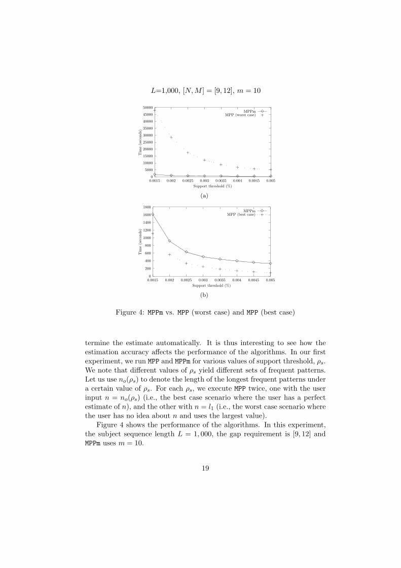
L=1,000, [N,M ] = [9, 12], m = 10

0

5000

10000

15000

20000

25000

30000

35000

40000

45000

50000

0.0015 0.002 0.0025 0.003 0.0035 0.004 0.0045 0.005

Tim

e(s

econ

ds)

Support threshold (%)

MPPm

33333333

3MPP (worst case)

++++

+

+

+

++

(a)

0

200

400

600

800

1000

1200

1400

1600

1800

0.0015 0.002 0.0025 0.003 0.0035 0.004 0.0045 0.005

Tim

e(s

econ

ds)

Support threshold (%)

MPPm

33333

3

3

33

MPP (best case)

++++++

+

+

+

(b)

Figure 4: MPPm vs. MPP (worst case) and MPP (best case)

termine the estimate automatically. It is thus interesting to see how theestimation accuracy affects the performance of the algorithms. In our firstexperiment, we run MPP and MPPm for various values of support threshold, ρs.We note that different values of ρs yield different sets of frequent patterns.Let us use no(ρs) to denote the length of the longest frequent patterns undera certain value of ρs. For each ρs, we execute MPP twice, one with the userinput n = no(ρs) (i.e., the best case scenario where the user has a perfectestimate of n), and the other with n = l1 (i.e., the worst case scenario wherethe user has no idea about n and uses the largest value).

Figure 4 shows the performance of the algorithms. In this experiment,the subject sequence length L = 1, 000, the gap requirement is [9, 12] andMPPm uses m = 10.

19

First, we observe from the figure that as the support threshold increases,the execution times of the algorithms decrease. This is because a larger ρs

gives fewer frequent patterns to extract. Also, from Figure 4(a), we see thatwithout a reasonable estimate of n, the performance of MPP (worst case) isvery bad. MPPm, on the other hand, is much more efficient due to its abilityto determine a much smaller n. As an example, when ρs = 0.003%3, theexperiment result shows that the longest frequent pattern has a length ofno(0.003%) = 13. While MPP uses n = l1 = 77, MPPm estimates a value of n =22. As we have explained in the previous section, a small value of n enablesa much better pruning condition when the algorithms are determining whichcandidate patterns in Ci should be collected in the set L̂i. It explains whyMPPm is much more efficient than MPP under the worst case.

Figure 4(b) compares MPPm against MPP when the user has a perfectestimate of n. From the figure, we see that MPPm is less efficient than MPP(best case). There are two reasons why MPPm takes longer time to execute.First, determining the value em (so that MPPm can apply Theorem 2 toestimate a value of n) requires MPPm to check quite a number of length-mpatterns in the subject sequence S (see the discussion preceding Theorem 2).This overhead is not required for MPP. Second, MPP (best case) uses a smaller(and accurate) n value than MPPm does. Pruning is thus more effective. Theperformance difference, however, is not as big as that between MPPm andMPP (worst case). For example, in the above experiments, MPPm is 1.5 to 3.7times slower than MPP (best case), and it is 16 to 30 times faster than MPP(worst case).

Our experiment result also shows that both MPP and MPPm are much moreefficient than the straight forward way of enumerating all candidates. Sincethe Apriori property does not hold, the enumeration algorithm has to countall possible candidates. In our experiment settings, the number of candidatescounted by the enumeration method is 4i for Ci . On the other hand, bothMPP and MPPm are able to prune a large number of candidates. Table 3shows the number of candidates processed by the enumeration algorithm,MPP (worst case), MPPm and MPP (best case), respectively. The enumerationalgorithm is impractical due to the large number of candidates it needs toprocess. The number of candidates MPP (worst case) has to deal with isalso large, however, it becomes computable. For MPPm, it counts much fewercandidates than MPP (worst case), which explains why MPPm is much fasterthan MPP (worst case). MPP (best case) processes even fewer candidates than

3Recall that a pattern P is frequent if sup(P ) ≥ Nlρs. Since Nl is exponentially largew.r.t. l, even a small ρs implies a fairly large support count of P .

20

Enumeration MPP MPPm MPPAlgorithm (worst case) (best case)

C3 64 64 64 64C4 256 256 256 256C5 1024 1024 1024 1024C6 4096 4096 4096 4096C7 16384 16384 16384 16384C8 65536 65528 54588 50609C9 262144 231161 17464 12198C10 1048576 177140 2926 2262C11 4194304 37543 1057 783C12 16777216 16114 346 222C13 413 7552 42 26C14 414 2919 6 3C15 415 1009 - -C16 416 356 - -C17 417 43 - -C18 418 8 - -C19 419 - - -...

......

......

C77 477 - - -

Table 3: Number of candidates counted by different algorithms

MPPm. Therefore it has the shortest execution time. The large differencebetween MPP (worst case) and MPP (best case) indicates that the efficiencyof the MPP algorithm is dominated by the user input n, the estimated lengthof the longest frequent patterns.

To further illustrate the effect of the user input n, we execute MPP overdifferent values of n. In this experiment no(ρs) = 13. Figure 5 shows theresult. As expected, the worse is the estimate (a larger n), the slower isMPP. What is interesting about this figure is the execution time of MPP whenn = 10, a value that is smaller than no(ρs), the length of the longest frequentpatterns in S. That is to say, when the user under-estimate no(ρs). Fromthe figure, we see that the execution time of MPP is smaller than the casewhen n equals the real maximum length no(ρs).

Recall that for a given user input n, MPP will find all frequent patterns oflengths less than or equal to n. For longer patterns, MPP takes a best-effort

21

L = 1, 000, [N,M ] = [9, 12], ρs = 0.003%

200

400

600

800

1000

1200

1400

1600

1800

2000

2200

10 20 30 40 50 60

Tim

e(s

econ

ds)

n

33

3

3

3

3

Figure 5: Performance of MPP under different user input n

approach and tries to return those frequent patterns as many as possible.Therefore, if n < no(ρs), not all frequent patterns are guaranteed to befound. The small execution time of MPP when n = 10 as shown in Figure 5,however, hints at an adaptive approach to determine a suitable n value.Specifically, if a user has no idea of a good n value, we could run MPP using asmall n, let’s say 10. After MPP finishes execution, it will return all frequentpatterns of length less than or equal to n plus a number of longer frequentpatterns. We could note the longest pattern discovered, use its length torefine n and re-execute MPP. This process could continue until we cannotrefine n further. Although we do not explore this approach further in thispaper, we remark that since the cost of running MPP with a small n is low,running it a few times adaptively as the way we just described could still bea very efficient method.

In another experiment, we study the effect of the flexibility of the gap W .We fix N = 9 and hence the gap requirement is [9 . . . W +8]. Figure 6 showsthe performance of MPPm when W changes from 4 to 8. From the figure, wesee that the larger is W , the larger is the execution time of the algorithm.This is because, for a given l, the number of length-l offset sequences, Nl,is proportional to W l−1 (see Section 4.1). That is, the larger the value ofW , the larger is Nl. Hence, the PIL lists with which the algorithm uses tocount patterns’ supports are long. Therefore, more computational effort isneeded. From the figure, we see that for MPPm (and MPP) to be practical,the gap flexibility, W , has to be reasonably small. Fortunately, the helicalstructure of DNA sequences does not imply a large flexibility. For example,in some organism, a helical turn consists of 10 to 11 base pairs, which implies

22

L = 1, 000, N = 9,m = 8, ρs = 0.003%

0

500

1000

1500

2000

2500

4 5 6 7 8

Tim

e(s

econ

ds)

W

3 3

3

3

3

Figure 6: Performance of MPPm under different values of W

L = 1, 000,W = 4,m = 8, ρs = 0.003%

330

340

350

360

370

380

390

400

8 9 10 11 12

Tim

e(s

econ

ds)

N

3

3

3

3

3

Figure 7: Performance of MPPm under different values of N

a flexibility of 2.In the next experiment, we fix the gap flexibility W to 4 and vary the

value of N . The gap requirement is thus [N,N + 3]. Figure 7 shows theperformance of MPPm as N varies from 8 to 12. From the figure, we see thatthe execution time of MPPm increases with N . Recall that after MPPm hasestimated a value of n, it basically follows the logic of MPP. In particular,during the iteration in which MPPm determines the set L̂i, a candidate patternin Ci is removed if its support ratio is less than λn,n−i · ρs. According to

Equation 4, λn,n−i = L−(n−1)(M+N2

+1)

L−(i−1)(M+N2

+1). One can verify that λn,n−i is a

decreasing function of N . Hence, the smaller the value of N , the largerλn,n−i is, and more candidate patterns can be pruned. This leads to a more

23

ρs = 0.003%, [N,M ] = [9, 12],m = 10

500

1000

1500

2000

2500

3000

1000 2000 3000 4000 5000 6000 7000 8000 9000 10000

Tim

e(s

econ

ds)

L

3

3

3

3

3

3

3

3

3

3

Figure 8: Performance of MPPm for various values of L

efficient algorithm.Our final experiment studies the scalability property of the algorithm.

Figure 8 shows the execution time of MPPm as the length of the subjectsequence (L) varies from 1,000 to 10,000 characters. The result shows thatMPPm scales linearly with the sequence length.

7 A Case Study

In this section we report a case study in which interesting patterns aremined using our algorithms. We applied MPPm to mine a number of DNAsequences, including the whole genomes of the bacteria H. influenzae, H.pylori, M. genitalium and M. pneumoniae. We segmented the genomes intoshort fragments of 100 kilo-bases (kb), and ran the algorithm on each frag-ment using a gap size of [10, 12] and a support threshold of 0.006%. Thelength of the longest patterns discovered was 10 bases (characters). Weobserved a very interesting result: the bases ‘A’ and ‘T’ constitute muchmore to the periodic patterns than ‘C’ and ‘G’. For instance, there are 256length-8 patterns that consist of only ‘A’s and ‘T’s. We found that all suchpatterns were frequent in some fragments of all four genomes. Some of thesepatterns were even frequent in every fragment examined. As an example, ifwe consider fragments from bacteria genomes only, then on average, about250 of the 256 length-8 patterns that consist of only ‘A’s and ‘T’s were fre-quent in a given fragment. On the other hand, length-8 patterns that consistof more than one ‘C’ or ‘G’ were unlikely to be frequent. For example, thereare 48 = 65, 536 possible length-8 patterns, among which 28 = 256 contain

24

only ‘A’s and ‘T’s, and 8 × 2 × 27 = 2, 048 contain exactly one ‘C’ or ‘G’.So, the number of possible patterns that have more than one ‘C’ or ‘G’is 65, 536 − 256 − 2, 048 = 63, 232. We found that among these patterns,on average, only 3.9 of them were frequent in a DNA fragment of bacteriagenomes. Also, none such frequent patterns is common in all genomes.

The results are consistent with the findings of a previous study [7], whichshows the periodic occurrence of ‘A’ and ‘T’ in yeast and various bacteriaand archaea with a period length of 10-11 base pairs. Our results comple-ment its findings by showing that beyond the regularity that occurs betweennucleotide pairs, the patterns actually last for quite a number of contiguouscycles. Also, some patterns are ubiquitous in the genomes, not restrictingto any specific regions.

In a previous work that extensively studies ApA dinucleotide periodicity(the regular occurrence of base ‘A’ after another base ‘A’ separated by a fixedperiod) in various eubacteria, archaebacteria, eukaryotes and organelles, ithas been suggested that the periodic patterns are more prominent in eu-bacteria than in eukaryotes [17]. For instance, the genome of H. sapiens(human) shows very weak periodicity, as compared to the eubacteria andsome lower eukaryotes such as the baker yeast S. cerevisiae. We would liketo verify whether the periodic patterns are really weakened in higher eukary-otes, or strong periodic patterns still exist, but they are composed of otherbases or do not exhibit a rigorous periodicity with a fixed period length.We downloaded short pieces of the genomes of the eukaryotes H. sapiens, C.elegans and D. melanogaster, cut them into 100kb fragments, and repeatedthe above experiments. To our surprise, all of the 256 length-8 patterns thatconsists of ‘A’ and ‘T’ only are still frequent in some fragments of all threesequences. This result may imply that the flexible gap requirement is ableto tolerate some variations in the sequences, such as the insertion or deletionof a nucleotide within a period that affects the period length.

Besides, some patterns not detected in the bacterial genomes are ob-served in the eukaryote sequences, many of which consist of more ‘C’s and‘G’s. For instance, the length-8 pattern composing of ‘G’s only is frequentin some fragments of all three sequences. In one of the fragments of H.sapiens, the pattern composing of 16 G’s only is also found to be frequent!All these suggest that the nucleotides involved in the periodic patterns inbacteria and eukaryotes are quite different.

Some former studies suggest two explanations for the dinucleotide os-cillations [18, 17, 7]: (1) they are related to the helical shape of the DNA.In particular, the repetition of specific base-pair stacks with this periodicitywould cause uni-directional deflection of the DNA curvature; (2) the alter-

25

nation of hydrophobic and hydrophilic amino acids in α-helices leads to aperiodicity of about 3.5 amino acids in protein sequences, which correspondsto 10-11 bases in DNA sequences. Both explanations are still possible giventhe new findings. The new results also further suggest that in eukaryotes, themaintenance of the DNA curvature may involve more ‘C’s and ‘G’s than inbacteria. Also, to verify the second explanation, it is useful to actually lookfor some proteins with a corresponding coding DNA sequence that exhibitsthe mined periodic patterns.

Finally, we have applied our algorithm on mining DNA sequences ofmany different species. We found that there are unique periodic patternsfor each species. Some of these patterns are very interesting. For example,for C. elegans, we found periodic patterns that repeat themselves, such asATATATATATA, GTAGTAGTAGT, etc. As another example, a unique periodicpattern for H. sapiens consists of 17 ‘G’s. Biologists may find those patternsinsightful.

8 Conclusion

This paper studied the problem of mining periodic patterns with a gaprequirement from sequences. We formally defined the data-mining modeland proved several important theorems that lead to the derivation of efficientalgorithms. We proposed two algorithms, namely, MPP and MPPm for solvingthe problem. Extensive experiments had been done to illustrate the variousperformance characteristics of the algorithms. We found that for cases inwhich the user has a good estimate of the length of the longest frequentpatterns, MPP is the most efficient algorithm. On the other hand, if the userdoes not provide the estimate, MPPm is able to determine a reasonably goodone. We applied MPPm on a number of real DNA sequences. Much of ourmining result is consistent with findings from previous studies.

References

[1] Stephen F. Altschul, Warren Gish, Webb Miller, Eugene W. Myers,and David J. Lipman. Basic local alignment search tool. Journal ofMolecular Biology, 215:403–410, 1990.

[2] A. Bairoch and B. Boeckmann. The swiss-prot protein sequence databank. Nucleic Acids Research, 20(Suppl):2019–2022, 1992.

26

[3] Giorgio Bernardi, Birgitta Olofsson, Jan Filipski, Marino Zerial,Julio Salinas, Gerard Cuny, Michele Meunier-Rotival, and FrancisRodier. The mosaic genome of warm-blooded vertebrates. Science,228(4702):953–958, 1985.

[4] Eivind Coward and Finn Drablos. Detecting periodic patterns in bio-logical sequences. Bioinformatics, 14(6):498–507, 1998.

[5] J. W. Fickett and C. S. Tung. Assessment of protein coding measures.Nucleuic Acids Research, 20:6441–6450, 1992.

[6] Jiawei Han, Guozhu Dong, and YiWen Yin. Efficient mining of partialperiodic patterns in time series database. In Proc. of 15th InternationalConference on Data Engineering, ICDE99, pages 106–115, 1999.

[7] H. Herzel, O. Weiss, and E. N. Trifonov. 10-11 bp periodicities incomplete genomes reflect protein structure and DNA folding. Bioinfor-matics, 15(3):187–193, 1999.

[8] Inge Jonassen. Efficient discovery of conserved patterns using a patterngraph. Technical Report Report No. 118, University of Bergen, 1996.

[9] Stefan Kurtz, Enno Ohlebusch, Chris Schleiermacher, Jens Stoye, andRobert Giegerich. Computation and visualization of degenerate repeatsin complete genomes. In Proceedings of the 8th International Conferenceon Intelligent Systems for Molecular (ISMB-00), 2000.

[10] H. Mannila, H. Toivonen, and A. I. Verkamo. Discovery of frequentepisodes in event sequences. Data Mining and Knowledge Discovery,1(3):259–289, Nov 1997.

[11] http://www.ncbi.nlm.nih.gov.

[12] Jian Pei, Jiawei Han, Behzad Mortazavi-Asl, Helen Pinto, QimingChen, Umeshwar Dayal, and Mei-Chun Hsu. Prefixspan: Mining se-quential patterns by prefix-projected growth. In Proc. 17th IEEE In-ternational Conference on Data Engineering (ICDE), Heidelberg, Ger-many, April 2001.

[13] T. Imielinski R. Agrawal and A. Swami. Mining association rules be-tween sets of items in large databases. In Proc. ACM SIGMOD Inter-national Conference on Management of Data, page 207, Washington,D.C., May 1993.

27

[14] P.S. Reddy and D.E. Housman. The complex pathology of trinucleotiderepeats. Current Opinion in Cell Biology, 9(3):364–372, 1997.

[15] Isidore Rigoutsos and Aris Floratos. Combinatorial pattern discoveryin biological sequences: the teiresias algorithm. Bioinformatics, 14(1),1998.

[16] Ramakrishnan Srikant and Rakesh Agrawal. Mining sequential pat-terns: Generalizations and performance improvements. In Proc. of the5th Conference on Extending Database Technology (EDBT), Avignion,France, March 1996.

[17] Masaru Tomita, Masahiko Wada, and Yukihiro Kawashima. ApA din-ucleotide periodicity in prokaryote, eukaryote, and organelle genomes.Journal of Molecular Evolution, 49:182–192, 1999.

[18] E. N. Trifonov. 3-, 10.5-, 200- and 400-base periodicities in genomesequences. Physica A, 249:511–516, 1998.

[19] A. van Belkum, S. Scherer amd W. van Leeuwen, D. Willemse, L. vanAlphen, and H. Verbrugh. Variable number of tandem repeats inclinical strains of haemophilus influenzae. Infection and Immunity,65(12):5017–5027, 1997.

[20] J. Widom. Short-range order in two eukaryotic genomes: Relation tochromosome structure. Journal of Moleular Biology, 259:579–588, 1996.

[21] Jiong Yang, Wei Wang, and Philip S. Yu. Mining asynchronous pe-riodic patterns in time series data. In Proceedings of the sixth ACMSIGKDD international conference on Knowledge discovery and datamining, pages 275–279, Boston, MA USA, 2000.

[22] Mohammed J. Zaki. Efficient enumeration of frequent sequences. InProceedings of the 1998 ACM 7th International Conference on Infor-mation and Knowledge Management(CIKM’98), Washington, UnitedStates, November 1998.

[23] Minghua Zhang, Ben Kao, C.L. Yip, and David Cheung. A GSP-based efficient algorithm for mining frequent sequences. In Proc. ofIC-AI’2001, Las Vegas, Nevada, USA, June 2001.

28

Appendix: Determining Nl

First, let i = maxspan(l) − L. Consider all length-l offset sequences of theform [c1 = 1, c2, . . . , cl] where cl ≤ L, i.e., those offset sequences with thefirst offset being ‘1’, the first position of the subject sequence s. Let us usef(l, i) to denote the number of such offset sequences.

If i ≤ 0, we have maxspan(l) ≤ L. So, if the first offset is 1, cl ≤ Leven if every gap takes on the maximum value M . Hence, we have Wchoices for each of the remaining l − 1 offsets, and f(l, i) = W l−1. Also, ifi > (l−1)(W −1), we have maxspan(l)−L > (l−1)(W −1), or equivalently,minspan(l) > L, In this case, the offset sequence exceeds the span of thesubject sequence even if every gap takes on the minimum value. Therefore,f(l, i) = 0. Hence,

f(l, i) = W l−1 (i ≤ 0) (6)f(l, i) = 0 (i > (l − 1)(W − 1)) (7)

The values of f(l, i) for other values of i are related by the equationspecified in the following theorem:

Theorem 3∑(l−1)(W−1)

i=1 f(l, i) = l−12 (W − 1)W l−1, for l > 1.

Proof:For l = 2, let us consider the length-2 offset sequence [1, c2]. Since the

second offset (i.e., c2) must be within bound (i.e., ≤ L) and the gap mustsatisfy the gap requirement (i.e., N ≤ c2 − 2 ≤ M), we have N + 2 ≤ c2 ≤min(M +2, L). Since i = maxspan(2)−L, we have i = (2− 1)M +2−L, orM+2 = L+i. Therefore, for 1 ≤ i ≤ M−N = W−1, the number of possiblevalues of c2 is L− (N +2)+1 = M +2− i−N −1 = M −N +1− i = W − i.Hence,

f(2, i) = W − i ∀1 ≤ i ≤ W − 1.

And thus

(2−1)(W−1)∑

i=1

f(2, i) = (W − 1) + (W − 2) + . . . + 2 + 1

=W (W − 1)

2

=2− 1

2(W − 1)W 2−1

So, Theorem 3 is true for l = 2.

29

L = maxspan (k+1) - i

M

N W

1 2 N+1+1 N+1+j. . .

M+1. . .

M+1+1 LOffset:

S:

N+1. . . . . .

possible values of c2

L - (N+j)

Figure 9: An illustration

Suppose Theorem 3 is true for l = k where k ≥ 2. We consider thecase for l = k + 1. Recall that f(k + 1, i) refers to the number of distinctoffset sequences of the form [1, c2, . . . , ck+1], where ck+1 ≤ L. Due to thegap requirement, we have c2 = (N +1)+ j where 1 ≤ j ≤ W (see Figure 9).Now, let us fix the value of j (and hence c2) and focus on the segment ofthe sequence s[c2 . . . L]. From Figure 9, we see that the number of distinctoffset sequences is equal to the number of ways of selecting k offsets withinthe segment s[c2 . . . L], which is of length L − (N + j), such that the gaprequirement is satisfied among the offsets and that the first offset is takenas c2. Since L = maxspan(k + 1) − i, we have the length of the segmentbeing maxspan(k + 1) − i − (N + j) = kM + (k + 1) − i − (N + j) =(k− 1)M + k− (i−W + j) = maxspan(k)− (i−W + j). Hence, the numberof such selections is equal to f(k, i − W + j). This leads to the followingrecurrence equation:

f(k + 1, i) =W∑

j=1

f(k, i−W + j). (8)

Now,

(k+1−1)(W−1)∑

i=1

f(k + 1, i)

=(k+1−1)(W−1)∑

i=1

W∑

j=1

f(k, i−W + j)

=k(W−1)∑

i=1

W∑

j=1

f(k, i−W + j)

30

=W∑

j=1

k(W−1)∑

i=1

f(k, i−W + j) (replace the order of i, j)

=W∑

j=1

k(W−1)−W+j∑

m=1−W+j

f(k,m) (by m = i−W + j)

Splitting j into 3 parts: j = 1, 2 ≤ j ≤ W − 1 and j = W , we have

(k+1−1)(W−1)∑

i=1

f(k + 1, i)

=1∑

j=1

k(W−1)−W+j∑

m=1−W+j

f(k, m) +W−1∑

j=2

k(W−1)−W+j∑

m=1−W+j

f(k, m)

+W∑

j=W

k(W−1)−W+j∑

m=1−W+j

f(k, m) (9)

By Equation 6, we get

1∑

j=1

k(W−1)−W+j∑

m=1−W+j

f(k, m)

=(k−1)(W−1)∑

m=2−W

f(k, m)

=0∑

m=2−W

f(k,m) +(k−1)(W−1)∑

m=1

f(k, m)

= (W − 1)W k−1 +(k−1)(W−1)∑

m=1

f(k, m) (10)

Since when 2 ≤ j ≤ W − 1, we have 1−W + j ≤ 0, (k− 1)(W − 1)+1 ≤k(W − 1)−W + j, by Equations 6 and 7,

W−1∑

j=2

k(W−1)−W+j∑

m=1−W+j

f(k,m)

=W−1∑

j=2

0∑

m=1−W+j

f(k,m) +W−1∑

j=2

(k−1)(W−1)∑

m=1

f(k, m)

31

+W−1∑

j=2

k(W−1)−W+j∑

m=(k−1)(W−1)+1

f(k,m)

=W−1∑

j=2

(W − j)W k−1 +W−1∑

j=2

(k−1)(W−1)∑

m=1

f(k,m) + 0

=(W − 2)(W − 1)

2W k−1 + (W − 2)

(k−1)(W−1)∑

m=1

f(k, m)

(11)

Also by Equation 7,

W∑

j=W

k(W−1)−W+j∑

m=1−W+j

f(k, m)

=k(W−1)∑

m=1

f(k, m)

=(k−1)(W−1)∑

m=1

f(k,m) +k(W−1)∑

m=(k−1)(W−1)+1

f(k, m)

=(k−1)(W−1)∑

m=1

f(k,m) + 0

=(k−1)(W−1)∑

m=1

f(k,m) (12)

Combing Equations 9, 10, 11 and 12, we get

(k+1−1)(W−1)∑

i=1

f(k + 1, i)

=1∑

j=1

k(W−1)−W+j∑

m=1−W+j

f(k,m) +W−1∑

j=2

k(W−1)−W+j∑

m=1−W+j

f(k, m)

+W∑

j=W

k(W−1)−W+j∑

m=1−W+j

f(k,m)

= (W − 1)W k−1 +(k−1)(W−1)∑

m=1

f(k,m)

32

+(W − 2)(W − 1)

2W k−1 + (W − 2)

(k−1)(W−1)∑

m=1

f(k,m)

+(k−1)(W−1)∑

m=1

f(k, m)

=W (W − 1)

2W k−1 + W

(k−1)(W−1)∑

m=1

f(k, m)

=12(W − 1)W k

+k − 1

2(W − 1)W k (by induction hypothesis)

=k + 1− 1

2(W − 1)W k+1−1

Hence, Theorem 3 is true for l = k + 1. By induction, Theorem 3 is true. 2

With Theorem 3, we are ready to determine Nl. We consider three cases.Case 1: l > l2. In this case, minspan(l) > L. That is, the minimum

span of any length-l pattern exceeds the length of the subject sequence. So,there are no length-l offset sequences, or Nl = 0.

Case 2: l ≤ l1. In this case, Nl is given by the following theorem.

Theorem 4 Given a sequence s of length L and a gap requirement [N, M ],if l ≤ l1, then Nl = [L− (l − 1)(M+N

2 + 1)]W l−1.

Proof: Let n(i) represent the number of distinct length-l offset sequences ofthe form [i, c2, . . . , cl] (i.e., the first offset equals i). We have Nl =

∑Li=1 n(i).

One can easily see that n(i) is equivalent to the number of distinct offsetsequences over a length-(L − (i − 1)) subject sequence with the first offsetbeing 1. Hence, n(i) = f(l,maxspan(l)− (L− i + 1)).

Since l ≤ l1, we have maxspan(l) ≤ L, so from Equations 6, 7 andTheorem 3,

Nl =L∑

i=1

n(i)

=L∑

i=1

f(l,maxspan(l)− (L− i + 1))

=maxspan(l)−1∑

i=maxspan(l)−L

f(l, i)

33

=0∑

i=maxspan(l)−L

f(l, i) +maxspan(l)−minspan(l)∑

i=1

f(l, i)

+maxspan(l)−1∑

i=maxspan(l)−minspan(l)+1

f(l, i)

=0∑

i=maxspan(l)−L

f(l, i) +(l−1)(W−1)∑

i=1

f(l, i)

+maxspan(l)−1∑

i=(l−1)(W−1))+1

f(l, i)

=0∑

i=maxspan(l)−L

W l−1 +l − 1

2(W − 1)W l−1

+maxspan(l)−1∑

i=(l−1)(W−1))+1

0

= (L−maxspan(l) + 1)W l−1 +l − 1

2(W − 1)W l−1

=[L− (l − 1)(

M + N

2+ 1)

]W l−1

2

Case 3: l1 < l ≤ l2. In this case, maxspan(l) > L. From Equation 7 wehave,

Nl =maxspan(l)−minspan(l)∑

i=maxspan(l)−L

f(l, i)

+maxspan(l)−1∑

i=maxspan(l)−minspan(l)+1

f(l, i)

=(l−1)(W−1)∑

i=maxspan(l)−L

f(l, i) +maxspan(l)−1∑

i=(l−1)(W−1)+1

0

=(l−1)(W−1)∑

i=maxspan(l)−L

f(l, i)

Although not a closed-form formula, we can compute Nl using Equation 8.

34