minimum wages and youth employment in france and … · minimum wages and youth employment in...
TRANSCRIPT

This PDF is a selection from an out-of-print volume from the National Bureauof Economic Research
Volume Title: Youth Employment and Joblessness in Advanced Countries
Volume Author/Editor: David G. Blanchflower and Richard B. Freeman,editors
Volume Publisher: University of Chicago Press
Volume ISBN: 0-226-05658-9
Volume URL: http://www.nber.org/books/blan00-1
Publication Date: January 2000
Chapter Title: Minimum Wages and Youth Employment in France and theUnited States
Chapter Author: John M. Abowd, Francis Kramarz, Thomas Lemieux, DavidN. Margolis
Chapter URL: http://www.nber.org/chapters/c6813
Chapter pages in book: (p. 427 - 472)

Minimum Wages and Youth Employment in France and the United States John M. Abowd, Francis Kramarz, Thomas Lemieux, and David N. Margolis
11.1 Introduction
In this paper we examine the link between changes in the minimum wage and employment outcomes for the youth (under age 31) labor mar- ket, in France and the United States. We make use of longitudinal data on employment status and earnings to see how individuals are affected by real increases (in the case of France) or real decreases (in the case of the United States) in the minimum wage conditional on the individual’s loca-
John M. Abowd is professor of labor economics at Cornell University, distinguished sen- ior research fellow at the U.S. Bureau of the Census, research associate at the Centre de Recherche en Economie et Statistique (CREST, Paris), and a research associate of the Na- tional Bureau of Economic Research. Francis Kramarz is head of the research department at INSEE-CREST, the French statistical institute; an associate professor at Ecole Polytech- nique; and a research fellow of the Centre for Economic Policy Research, London. Thomas Lemieux is associate professor of economics at the University of British Columbia, a re- search director of the Centre Interuniversitaire de Recherche en Analyse des Organisations (CIRANO, Montreal), and a research associate of the National Bureau of Economic Re- search. David N. Margolis is a researcher with the Centre National de la Recherche Scienti- fique, working at the Universitt de Paris 1 Pantheon-Sorbonne in the Laboratoire de Micro- Cconomie Appliqube and the Centre de Recherche en Economie et Statistique. Part of this paper was written while Margolis was assistant professor at the Universitb de Montreal and a research associate at the Centre de Recherche et Developement en Economie and the Centre Interuniversitaire de Recherche et d’Analyse des Organisations.
The authors gratefully acknowledge financial support from CIRANO, the National Sci- ence Foundation (SBR-93-21053 to Abowd and Margolis), and the Fonds pour la Formation de Chercheurs et ]’Aide a la Recherche (97-NC-1676 to Margolis). Much of this work was completed while Margolis was visiting the CREST Laboratoire de Microeconomttrie. The authors thank David Blanchflower, Richard Freeman, Shulamit Kahn, Lawrence Katz, Alan Krueger, John Martin, and participants at the NBER Summer Institute, CIRANO Summer Workshop, CREST Departement de la Recherche Internal Workshop, CREST Microecono- mttrie Workshop, and the Universiti de Paris 1 Pantheon-Sorbonne for comments on pre- vious versions of this paper. The American data used in this study were taken from public-
427

428 J. M. Abowd, F. Kramarz, T. Lemieux, and D. N. Margolis
tion in the earnings distribution. We take particular care to distinguish subpopulations that might be affected differently by the minimum wage, focusing in particular on low-wage workers and (in the case of France, where the data are available) on the use of employment promotion con- tracts that allow the payment of subminimum wages.
Although little attention has been paid to the situation in Europe,' some European countries provide interesting alternatives to the much studied U.S. case. France, in particular, seems a perfect contrast to the United States. Whereas in the United States the nominal federal minimum wage remained constant for most states during most of the 1980s (thus implying a declining real federal minimum wage), nominal minimum wages in France rose steadily over the 1980s, as did real minimum wages. In this paper we exploit the different growth patterns in real minimum wages in a symmetric manner to more clearly understand their effect on employment.
Most existing studies of the French minimum wage system use aggre- gate time-series data and find no effect of the minimum wage system on youth employment (see, e.g., Bazen and Martin 1991). This is surprising because, since the inception of the minimum wage, a significant percent- age of the French labor force has been employed at wages close to that level. One reason for the orientation in the empirical analyses done in France is, certainly, the tendency of American applied researchers to rely on aggregate time-series analyses' prior to the widespread dissemination of public-use microeconomic data such as the Current Population Survey (CPS). Another reason is that research access to French microdata was extremely limited until the 1990s. In the present study we use microdata from France and the United States collected in household surveys that are quite comparable. In particular, we use longitudinal information on the workers. Consequently, we are able to analyze both French and American minimum wage systems using individual-level panel data.
Because of the dramatic differences between the evolution of both nom- inal and real French minimum wages and that of the national US. mini- mum,3 we have designed statistical comparisons that address the same be-
use Current Population Survey (CPS) files provided by the Bureau of Labor Statistics and the Bureau of the Census. David Card graciously provided the computer code for implement- ing the Census Bureau CPS matching algorithms used in this paper. The French data were taken from the Enqucte Emploi research files constructed by the Institut National de la Statistique et des Etudes Economiques (INSEE, the French national statistical agency). The French data are also public-use samples. For further information contact INSEE, Dkpdrte- ment de la Diffusion, 18 bd Adolphe Pinard, 75675 Paris Cedex 14, France. The opinions expressed in this paper are those of the authors, not the U.S. Census Bureau. The paper was completed before Abowd assumed his appointment.
1. See Dolado et al. (1996) for a summary of minimum wage studies for France, the Neth- erlands, Spain, and the United Kingdom.
2. See Brown, Gilroy, and Kohen (1982) for a review. 3. We do not consider state-specific minimum wages or youth subminimum wages in the
United States, which became increasingly important at the end of the 1980s. See Neumark

Minimum Wages and Youth Employment in France and the U.S. 429
havior using the different variations in the national minimum wage systems to identify the relevant effects. We use two different statistical ap- proaches based on the same idea: analysis of employment transition prob- abilities conditional on the position of an individual in the wage distri- bution. In each approach, we decompose the wage distribution into four components (under, around, marginally over, and over the minimum wage). We then, in our first approach, use a multinomial logit model to analyze the factors that affect the probability of making a transition be- tween a particular position in the wage distribution and employment or nonemployment (in the case of France) or between employment or non- employment and the position in the wage distribution (in the case of the United States). We find that young workers paid around the minimum wage in France were more likely to transition to a nonemployment state (unemployment or inactivity) than those paid over the minimum wage and that, for French men, such differences were greater in years where major increases in the minimum wage occurred. In the United States, we find that among workers currently employed around the minimum wage, a larger share were in a nonemployment state the previous period than among workers above the minimum wage. In both cases, the effects are strongest for the youngest workers. We find some minor “spillover” effects in both cases and provide evidence to suggest that these effects capture some of the heterogeneity between low-wage and high-wage labor markets.
In the second approach, we exploit the size of the movements in the real minimum wage more d i re~t ly .~ For France, we use the automatic and legislated increases in the nominal minimum wage that occur (at least) each July to identify groups of workers whose current wage rate will fall below the new minimum wage rate after the increase. We also identify workers whose present employment is part of a special youth program that permits wage payments below the statutory minimum. We use the limited duration of employment spells in such programs to identify a sec- ond group of minimum wage employment effects. Our statistical analysis identifies the change in future employment probabilities given an individu- al’s minimum wage status in the present period. We show that individuals whose reference year wage was between the two real minimum wages, as defined above, have substantially lower subsequent employment probabili- ties than those who were not. The conditional elasticity of subsequent nonemployment as a function of the real minimum wage for young male workers in France in this situation, evaluated at sample means, is -2.5. This effect is present even when unobserved labor market heterogeneity
and Wascher (1992) for an explicit treatment of this variation in the U.S. data. Similarly, we do not explicitly control for minimum wages specified by collective agreement in France that exceed the national minimum. See Margolis (1993) for a detailed treatment of the effects of the collective bargaining agreement salary grids on employment.
4. Our analysis bears some resemblance to that of Linneman (1982).
430 J. M. Abowd, F. Kramarz, T. Lemieux, and D. N. Margolis
and supply behavior are partially controlled for by the inclusion of a sepa- rate category for workers marginally over the minimum. However, the im- pact of the minimum wage decreases with experience. We also show that youths who participated in employment programs had lower subsequent employment probabilities. For the United States we use the constancy of the nominal minimum wage between 1981 and 1987 to identify groups of employed workers whose real wage in the present period would have been below the real minimum wage in the previous period. We show that young men whose wages were between the two real minimum wages, as described above, had lower employment probabilities in the previous period than individuals who were not (the conditional elasticity, evaluated at sample means, is 2.2). These effects get worse with age in the United States and are mitigated by eligibility for special employment promotion contracts in France.
The structure of this paper is as follows. Section 1 1.2 provides some in- stitutional background on the systems of minimum wages in both France and the United States and provides some preliminary indications of the potential impact in each case based on empirical wage distributions. Sec- tion 1 1.3 describes the data that we use to analyze the impact of minimum wages, and section 11.4 lays out the statistical models used to evaluate the employment effects of minimum wage changes. Section 11.5 details the results of our multinomial logit analysis, and section 11.6 discusses the conditional logit analyses. Section 1 1.7 concludes.
11.2 Institutional Background
1 1.2.1 France
The first minimum wage law in France was enacted in 1950, creating a guaranteed hourly wage rate that was partially indexed to the rate of in- crease in consumer prices. Beginning in 1970, the original minimum wage law was replaced by the current system (called the salaire minimum inter- professionnel de croissance-SMIC) linking the changes in the minimum wage to both consumer price inflation and growth in the hourly blue-collar wage rate. In addition to formula-based increases in the SMIC, the govern- ment legislated increases many times over the next two decades. The statu- tory minimum wage in France regulates the hourly regular cash compen- sation received by an employee, including the employee’s part of any payroll taxes.5
5. In theory, no provisions in any of the minimum wage laws allow regional variation in the SMIC. In some sectors in the French economy, however, the effective minimum wage was determined by (often extended) collective bargaining agreements. These agreements typically covered entire regions and industries, especially when extended to nonbargaining employers. Although relatively important in the 1970s, these provisions became increasingly irrelevant

Minimum Wages and Youth Employment in France and the US. 431
8000 ........................................................................................ F
Fig. 11.1 Monthly minimum wage: France
Figure 1 1.1 shows the time series for the French minimum wage and the associated employee-paid and employer-paid payroll taxes. Because of the extensive use of payroll taxes to finance mandatory employee benefits, by the 1980s the French minimum wage imposed a substantially greater cost on the employer than its statutory value. Employees share in the legal allocation of the payroll taxes, as the figure shows; however, low-wage workers benefit substantially more than the average worker from the social security systems financed through these taxes in proportion to their reve- nue (unemployment insurance, health care, retirement income, and em- ployment programs, in particular). Appendix table 1 1A. 1 provides a com- plete statistical history of the real and nominal SMIC, including employer and employee payroll tax components.
Figure 11.2 shows the real hourly French minimum wage from 1951 to 1994. Although the original minimum wage program (called the suluire minimum interprofessionnel gurunti-SMIG) was only partially indexed- in particular the inflation rate had to exceed 5 percent per year (2 percent from 1957 to 1970) to trigger the indexation-the real minimum wage did not decline measurably over the entire postwar period and increased substantially during most decades.
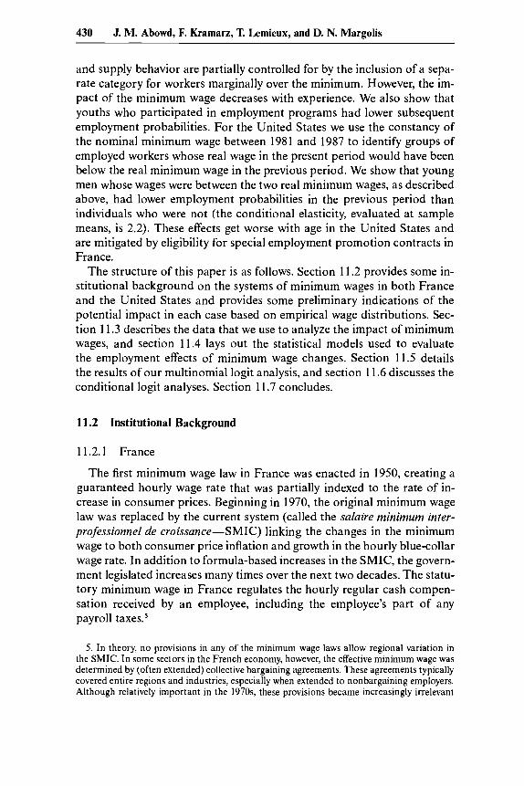
The French minimum wage lies near most of the mass of the wage rate distribution for the employed workforce. To show the location of the SMIC in this distribution, we plotted the empirical distribution of hourly
during the 1980s (our period of analysis) as the collective agreement nominal salary grids remained fixed in the face of an increasing nominal SMIC. See Margolis (1993) for a discus- sion of extended collective agreements and their relation to the SMIC.

432 J. M. Abowd, F. Kramarz, T. Lemieux, and D. N. Margolis
7.00 -
Y)
P
.c C
wage rates for 1990, the earliest year for which the Labor Force Survey reports continuous wage data. Figure 1 1.3 shows these data. We have indi- cated the SMIC directly on the figure. Notice that the first mode of the wage distribution is within F 5 of the minimum wage and the second mode is within F 10 of the minimum. In the overall distribution, 13.6 percent of the wage earners lie at or below the minimum wage and an additional 14.4 percent lie within an additional F 5 per hour of the SMIC.
Dolado et al. (1996) discuss the incidence of the SMIC with respect to household income. They find that although people employed at the SMIC do tend to be in the poorest households, the distribution of “smicards” (people paid the SMIC) is not monotonically decreasing in household income. For example, they find that the share of individuals paid the SMIC in each decile of household income increases from 10.1 percent in the lowest decile to 13.1 percent in the third lowest decile, then decreases to 6.6 percent for the fifth decile, increases to 7.4 percent for the sixth decile and declines monotonically to 0.6 percent in the highest decile of household income.
1 1.2.2 United States
The first national minimum wage in the United States was a part of the original Fair Labor Standards Act (FLSA) of 1938. The American na- tional minimum wage has never been indexed and increases only when legislative changes are enacted. The national minimum applies only to workers covered by the FLSA, whose coverage has been extended over the years to include most jobs. The statutory minimum wage regulates the
Minimum Wages and Youth Employment in France and the U.S. 433
Hourly wage rate net of employee payroll taxes (francs)
Fig. 11.3 Empirical distribution of hourly wages: France, 1990
Hourly wage rate including employee payroll taxes (dollars)
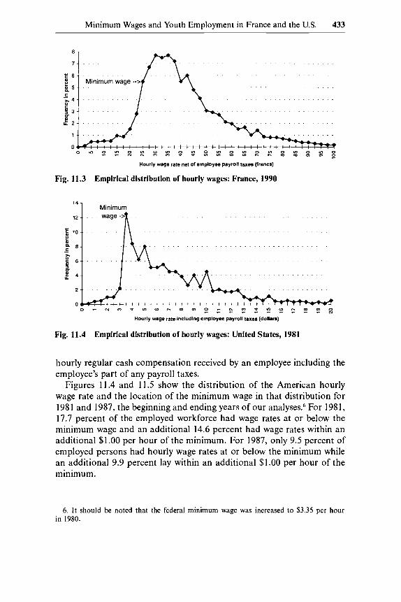
Fig. 11.4 Empirical distribution of hourly wages: United States, 1981
hourly regular cash compensation received by an employee including the employee's part of any payroll taxes.
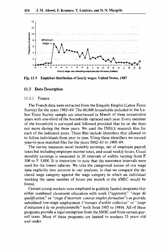
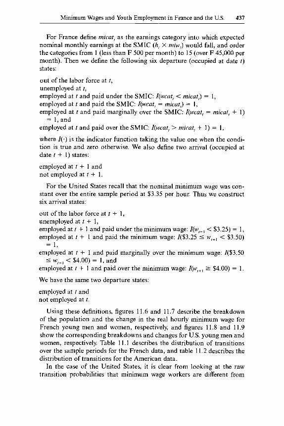
Figures 11.4 and 11.5 show the distribution of the American hourly wage rate and the location of the minimum wage in that distribution for 1981 and 1987, the beginning and ending years of our analyses.6 For 1981, 17.7 percent of the employed workforce had wage rates at or below the minimum wage and an additional 14.6 percent had wage rates within an additional $1.00 per hour of the minimum. For 1987, only 9.5 percent of employed persons had hourly wage rates at or below the minimum while an additional 9.9 percent lay within an additional $1.00 per hour of the minimum.
6. It should be noted that the federal minimum wage was increased to $3.35 per hour in 1980.
434 J. M. Abowd, F. Kramarz, T. Lemieux, and D. N. Margolis
5 1 0 -
8 -. Min imum
o - ” ~ ‘ ~ “ ” m ” n = “ 9 f ~ ~ S ~ ~ R Hourly wage rate Including employee payroll taxes (dollars)
Fig. 11.5 Empirical distribution of hourly wages: United States, 1987
11.3 Data Description
11.3.1 France
The French data were extracted from the EnquCte Emploi (Labor Force Survey) for the years 1982-89. The 60,000 households included in the La- bor Force Survey sample are interviewed in March of three consecutive years with one-third of the households replaced each year. Every member of the household is surveyed and followed provided that he or she does not move during the three years. We used the INSEE research files for each of the indicated years. These files include identifiers that allowed us to follow individuals from year to year. Using these identifiers we created year-to-year matched files for the years 1982-83 to 1988-89.
The survey measures usual monthly earnings, net of employee payroll taxes but including employee income taxes, and usual weekly hours. Usual monthly earnings is measured in 20 intervals of widths varying from F 500 to F 5,000. It is important to note that the narrowest intervals were used for the lowest salaries. We take the categorical nature of our wage data explicitly into account in our analyses, in that we compare the de- clared wage category against the wage category in which an individual working the same number of hours per month at the SMIC would be found.
Certain young workers were employed in publicly funded programs that either combined classroom education with work (“upprentis,” “stuge de quul@cution,” or “stage dinsertion, contrut emploi-formation”) or provide subsidized low-wage employment (“truvaux dutilitk collective” or “stuge dinitiution a la vieprofessionnelle,” both from 1985 to 1989). All of these programs provide a legal exemption from the SMIC and from certain pay- roll taxes. Most of these programs are limited to workers 25 years old and under.

Minimum Wages and Youth Employment in France and the US. 435
The employment status in year t is equal to one for all individuals who are employed in March of the survey year and equal to zero otherwise. The French Labor Force Survey definition of employment is the same as the one used by the International Labour Office: a person is employed if he or she worked for pay for at least one hour during the reference week. The definition is thus consistent with the American Bureau of Labor Sta- tistics (BLS) definition used below.
Our control variables consisted of education, labor force experience, seniority, region of France, date of labor force entry, and year. Education was constructed as eight categories: none, completed elementary school, completed junior high school, completed basic vocational/technical school, completed advanced vocational/technical school, completed high school (baccafaurgat), completed technical college or undergraduate uni- versity, and completed graduate school or postcollege professional school. Labor force experience was computed as the difference between current age and age at school exit. Seniority was measured as the response to a direct question on the survey (years with the present employer). Region is an indicator variable for the Ile de France (Paris metropolitan area) as the region of residence.
The SMIC data were taken from Bayet (1994), which reports official INSEE statistics. We selected the hourly SMIC for March of the indicated year, net of employee payroll taxes.
1 1.3.2 United States
We used the official BLS public-use outgoing rotation group files from the CPS for the months January to May and September to December and the years 1981-87. We applied the Census Bureau matching algorithm to create year-to-year linked files for the years 1981-82 to 1986-87.
The outgoing rotation groups (households being interviewed for the fourth or eighth time in the CPS rotation schedule) are asked to report usual weekly wage and usual weekly hours. Individuals who normally are paid by the hour are asked to report that wage rate directly. We created an hourly wage rate using the directly reported hourly wage rate when avail- able and the ratio of usual weekly earnings to usual weekly hours other- wise. Respondents are asked to report these wage measures gross of em- ployee payroll taxes, so they are not directly comparable to the measures constructed from the French data, which are reported net of employee payroll taxes. We created real hourly wage rates by dividing by the 1982-84-based Consumer Price Index for All Urban Workers for the ap- propriate month.
We created a second set of hourly wage measures for the United States that included income from tips in the hourly wage. To do this we computed a second hourly wage rate as usual weekly earnings divided by usual weekly hours for workers who reported that they were paid by the hour.

436 J. M. Abowd, F. Kramarz, T. Lemieux, and D. N. Margolis
When this second hourly wage rate exceeded the one directly reported, we used the computed measure. This measure of hourly wage rate is used below in the analysis labeled “including income from tips.”
An individual is employed in year t if he or she worked at least one hour for pay during the second week of the survey month. We used the CPS employment status recode variable to determine employment. The BLS definition is thus consistent with the one used in the French Labor Force Survey.
Our control variables consist of education, potential labor force experi- ence, race, marital status, and region. Education was constructed as the number of years required to reach the highest grade completed. For the multinomial logit analysis, this was decomposed into six categories: less than junior high school (no diploma), junior high school, high school, less than four years of college, four years of college, and more than four years of college. Potential labor force experience is age minus years of education minus five. Race is one for nonwhite individuals. Marital status is one for married persons. Region is a set of three indicator variables for the northeastern, north-central, and southern parts of the United States.
The U.S. national nominal minimum wage was $3.35 throughout our analysis period.’
1 1.3.3 Empirical Transition Probabilities
A preliminary analysis of the empirical transition probabilities of young workers into or out of employment based on their positions in the wage distribution relative to the minimum wage suggests that one might expect to see significant impacts of the minimum wage on employment probabili- ties in both France and the United States. In the case of France, we are concerned with that probability that an individual is employed at the date t + 1 given the person’s employment status and wage rate relative to the SMIC (if employed) at date t . In the case of the United States, the question is whether or not an individual was employed at date t given his or her employment status and wage rate relative to the minimum wage (if em- ployed) at date t + 1.
Let miw, be the nominal hourly minimum net wage in year t , rmiw, be the real hourly minimum net wage in year t, and h, represent the number of monthly hours worked in the sample month in year t . For France let wcut, be the category in which the individual’s nominal net monthly earn- ings falls in year t , and for the United States let w, be the individual’s hourly net wage rate in year t and rw, be the real net wage for year t .
7. Throughout the period, and particularly toward the end, some states independently increased their nominal wages above the national level. We do not explicitly account for state-by-state variation in the nominal minimum wage. See Neumark and Wascher (1992) for an analysis, using a different methodology, of the effects of interstate variation of mini- mum wages in the United States.
Minimum Wages and Youth Employment in France and the U.S. 437
For France define micat, as the earnings category into which expected nominal monthly earnings at the SMIC (h, X miw,) would fall, and order the categories from 1 (less than F 500 per month) to 15 (over F 45,000 per month). Then we define the following six departure (occupied at date t ) states:
out of the labor force at t , unemployed at t , employed at t and paid under the SMIC: Z(wcat, < micat,) = 1, employed at t and paid the SMIC: Z(wcat, = micat,) = 1, employed at t and paid marginally over the SMIC: Z(wcat, = micat, + 1)
employed at t and paid over the SMIC: Z(wcat, > micat, + 1) = 1,
where I ( - ) is the indicator function taking the value one when the condi- tion is true and zero otherwise. We also define two arrival (occupied at date t + 1) states:
employed at t + 1 and not employed at t + 1.
For the United States recall that the nominal minimum wage was con- stant over the entire sample period at $3.35 per hour. Thus we construct six arrival states:
out of the labor force at t + 1, unemployed at t + 1, employed at t + 1 and paid under the minimum wage: Z(wltl < $3.25) = 1, employed at t + 1 and paid the minimum wage: Z($3.25 5 w,,, < $3.50)
employed at t + 1 and paid marginally over the minimum wage: 1($3.50
employed at t + 1 and paid over the minimum wage: Z ( W , + ~ L $4.00) = 1.
We have the same two departure states:
employed at t and not employed at t.
Using these definitions, figures 11.6 and 11.7 describe the breakdown of the population and the change in the real hourly minimum wage for French young men and women, respectively, and figures 11.8 and 11.9 show the corresponding breakdowns and changes for U.S. young men and women, respectively. Table 1 1.1 describes the distribution of transitions over the sample periods for the French data, and table 11.2 describes the distribution of transitions for the American data.
In the case of the United States, it is clear from looking at the raw transition probabilities that minimum wage workers are different from
= 1, and
= 1,
5 w , , ~ < $4.00) = 1, and

438 J. M. Abowd, F. Kramarz, T. Lemieux, and D. N. Marpolis
0.S
0.15. : 0.1 p
- I 0 5
0.05
Fig. 11.6 young men
Population breakdown by earnings and evolution of real SMIC: French
0 1982 1983 1984 1985 1986 1987 1981
Y U ,
Fig. 11.7 Population breakdown by earnings and evolution of real SMIC: French young women
their higher paid counterparts. A much larger share of the population em- ployed at the minimum wage at date t + 1 comes from the nonworking pool (42.92 percent) than does the share of the population employed far over the minimum wage (only 12.28 percent). The case in France is less clear, since the difference between the share of workers paid at the SMIC who are not employed the following period (6.63 percent) and the share paid over the SMIC who are not employed the following period (12.16 percent) is much less dramatic, and even goes in the opposite direction from the U.S. result. These effects may, however, be due to the presence of various sorts of employment promotion contracts, which might shield workers paid at or under the SMIC from layoffs. Such effects would not

Minimum Wages and Youth Employment in France and the U.S. 439
I 1.m
4 / 4.16 ” I ,1. _ -
1982 1983 1984 1985 1986 1987
Y a I
Fig. 11.8 Population breakdown by earnings and evolution of real minimum wage: US. young men
8 5 I 7
~- om
r 0 2
I982 1983 1984 1985 1996 1981 Y..,
Fig. 11.9 Population breakdown by earnings and evolution of real minimum wage: U.S. young women
be visible in these cross-tabulations, and our conditional logit results go to great lengths to try to discriminate between the effects of the contracts and the effects of the minimum wage.
It should be noted that the transition behavior of workers paid margin- ally over the minimum is, in both countries, intermediate between the tran- sitions made by those paid at the minimum and those paid over the mini- mum. This “spillover” effect could be capturing a degree of heterogeneity between low-wage and high-wage workers, and we will exploit this control group in what follows.
Clearly, this descriptive analysis is not sufficient to discredit the hypoth- esis that low-wage workers are, in some way, qualitatively different from high-wage workers; in fact, the spillover effect noted above suggests that
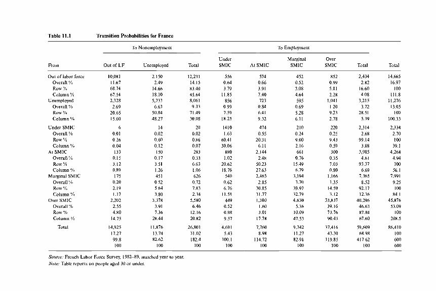
Table 11.1 Transition Probabilities for France
To Nonemployment To Employment
Under Marginal Over From Out of LF Unemployed Total SMIC At SMlC SMIC SMIC Total Total
Out of labor force Overall Yl, Row ‘7’0 Column ‘YO
Unemployed Overall 1%
ROW ‘Yo
Column I%
Under SMlC Overall ‘YO
Column ‘Yu
Overall (Yo
Row ‘% Column ’%
Marginal SMIC Overall 1%
ROW ‘Yo
Column <YO Over SMlC
Overall ‘Yu
Column ‘YO
Total
ROW%
At SMlC
ROW ‘Yo
10,081 1 I .67 68.74 67.54 2,328 2.69
20.65 15.60
6 0.01 0.26 0.04 133
0.15 3.12 0.89 175
0.20 2.19 1.17
2,202 2.55 4.80
14.75
14,925 17.27 99.8 100
2,150 2.49
14.66 18.10 5,733 6.63
50.84 48.27
14 0.02 0.60 0.12 150
0.17 3.51 1.26 451
0.52 5.64 3.80
3.378 3.91 7.36
28.44
11,876 13.74 82.62
100
12,231 14.15 83.40 45.64 8,061 9.33
71.49 30.08
20 0.02 0.86 0.07 283 0.33 6.63 I .06 626
0.72 7.83 2.34
5,580 6.46
12.16 20.82
26,801 31.02 182.4
100
556 0.64 3.79
11.85 856
0.99 7.59
18.25
1410 1.63
60.41 30.06
880 1.02
20.62 18.76
540 0.62 6.76
11.51 449 0.52 0.98 9.57
4,691 5.43
100.1 I00
574 0.66 3.91 7.40 723
0.84 6.41 9.32
474 0.55
20.31 6.1 1
2,144 2.48
50.23 27.63 2,465 2.85
30.85 31.77 1,380
1.60 3.01
17.78
7,760 8.98
114.72 100
452 0.52 3.08 4.64 595
0.69 5.28 6.11
210 0.24 9.00 2.16 661
0.76 15.49 6.79
3,194 3.70
39.97 32.79 4,630
5.36 10.09 47.53
9,742 11.27 82.91
100
852 0.99 5.81 2.28
1,041 I .20 9.23 2.78
220 0.25 9.43 0.59 300
0.35 7.03 0.80
1,166 1.35
14.59 3.12
33,837 39.16 73.76 90.43
37,416 43.30
119.85 100
2,434 14,665 2.82 16.97
16.60 I00 4.08 111.8
3,215 1 1,276 3.72 13.05
28.51 100 5.39 100.33
2,314 2,334 2.68 2.70
99.14 I00 3.88 39.1
3,985 4,268 4.61 4.94
93.37 100 6.69 56.1
7,365 7,991 8.52 9.25
92.17 100 12.36 84. I
40,296 45,876 46.63 53.09 87.84 I00 67.60 208.5
59,609 86,410 68.98 100
417.62 600 100 600
Source. French Labor Force Survey, 1982-89, matched year to year. Nore: Table reports on people aged 30 or under.
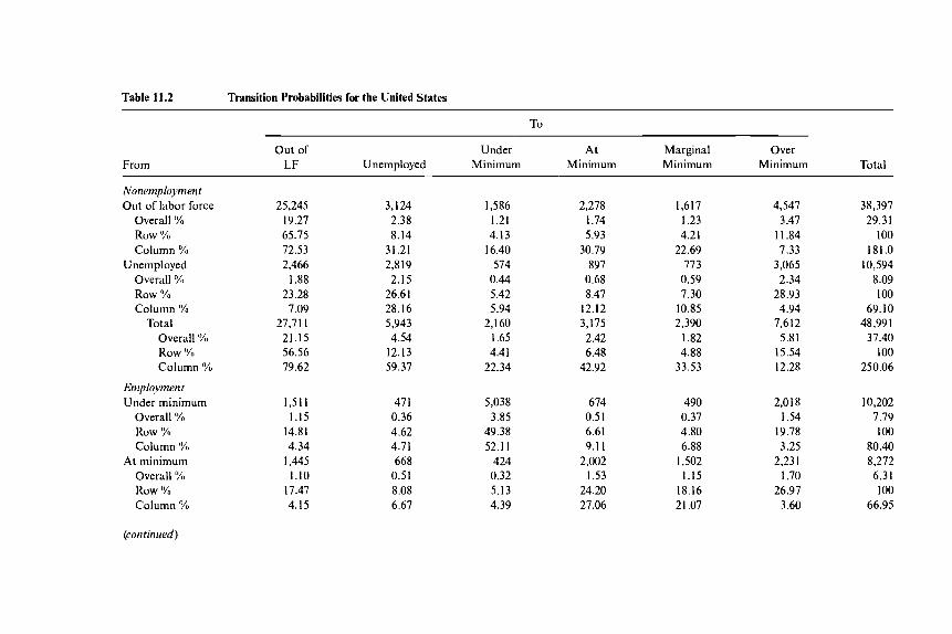
Table 11.2 Transition Probabilities for the United States
To
From o u t of Under At Marginal Over
LF Unemployed Minimum Minimum Minimum Minimum Total
Nonemployment Out of labor force
Overall %
Column YO Unemployed
Overall YO
Column 'Y Total
ROW 'Yo
ROW 'Yo
Overall 'YO
Column '% ROW Y o
Employment Under minimum
Overall I%
Column '% At minimum
Overall 'YO Row % Column 'Y
ROW 'Yo
25,245 19.27 65.75 72.53 2,466
I .88 23.28
7.09 27,71 I
21.15 56.56 79.62
1,511 1.15
14.81 4.34
1,445 1.10
17.47 4.15
3,124 2.38 8.14
31.21 2,819
2.15 26.61 28.16 5,943 4.54
12.13 59.37
47 1 0.36 4.62 4.71 668
0.51 8.08 6.67
1,586 1.21 4.13
16.40 574
0.44 5.42 5.94
2,160 1.65 4.41
22.34
5,038 3.85
49.38 52.1 1
424 0.32 5.13 4.39
2,278 1.74 5.93
30.79 897
0.68 8.47
12.12 3,175 2.42 6.48
42.92
674 0.51 6.61 9.1 1
2,002 1.53
24.20 27.06
1,617 I .23 4.21
22.69 773
0.59 7.30
10.85 2,390
1.82 4.88
33.53
490 0.37 4.80 6.88
1,502 1.15
18.16 21.07
4,547 3.47
11.84 7.33
3,065 2.34
28.93 4.94
7,6 12 5.81
15.54 12.28
2,O 18 I .54
19.78 3.25
2,231 1.70
26.97 3.60
38,397 29.31
100 181.0
10,594 8.09 100
69.10 48,991
37.40 100
250.06
10,202 7.79 100
80.40 8,272
6.31 100
66.95
(continued)
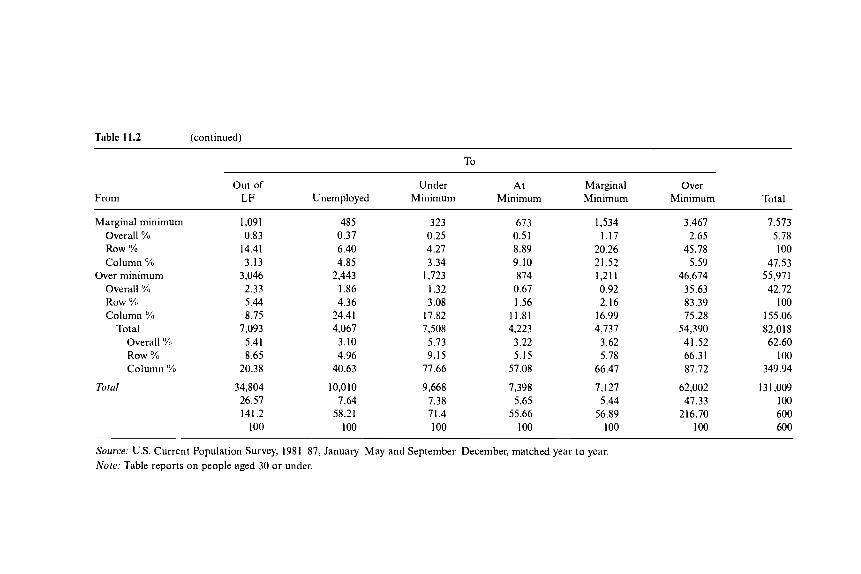
Table 11.2 (continued)
To
o u t of Under At Marginal Over From LF Unemployed Minimum Minimum Minimum Minimum Total
Marginal minimum 1,09 1 485 323 673 1,534 3,467 7,573 OVerdll Yo 0.83 0.37 0.25 0.5 1 1.17 2.65 5.78 Row Ya 14.41 6.40 4.27 8.89 20.26 45.78 100 Column YO 3.13 4.85 3.34 9.10 21.52 5.59 47.53
Over minimum 3,046 2,443 1,123 874 1,211 46,674 55,971 Overall YO 2.33 1.86 1.32 0.67 0.92 35.63 42.72 Row Yo 5.44 4.36 3.08 1.56 2.16 83.39 I00 Column YO 8.75 24.41 17.82 11.81 16.99 75.28 155.06
Total 7,093 4,067 7,508 4,223 4,737 54,390 82,018 Overall 'YO 5.41 3.10 5.73 3.22 3.62 41.52 62.60 Row %1 8.65 4.96 9.15 5.15 5.78 66.31 100 Column 'Yu 20.38 40.63 77.66 57.08 66.41 87.72 349.94
Total 34,804 10,010 9,668 7,398 1,127 62,002 131,009 26.57 7.64 7.38 5.65 5.44 47.33 100 141.2 58.21 71.4 55.66 56.89 2 16.70 600
100 100 100 100 100 I00 600
Source: US. Current Population Survey, 1981-87, January-May and September-December, matched year to year. Note: Table reports on people aged 30 or under.
Minimum Wages and Youth Employment in France and the U.S. 443
such heterogeneity may exist. To separate out this effect, we need to con- trol for worker characteristics and analyze more carefully the transitions between employment and nonemployment.*
11.4 Statistical Models for the Minimum Wage Effects on Employment
In order to control for the impact that variables, including the minimum wage and its movements, might have on labor market transitions, we ap- plied two different statistical techniques. In the first approach, we use a multinomial logit analysis to try to control for factors that might render low-wage workers different from other workers and could thereby affect their transition probabilities. We analyze the raw transitions and describe the factors that increase or reduce the probability of transitions involving nonemployment and how these factors differentially affect minimum wage and above minimum wage workers. In the second approach, we exploit the size of the increases to categorize workers as “between” old and new values of the real minimum wage (i.e., with an hourly real wage rate lying between the old and the new real minimum wage), and we use a logit analysis of subsequent (or prior) employment probabilities to see if work- ers who might be directly affected by minimum wage increases have sig- nificantly different subsequent (or prior) employment probabilities.
1 1.4.1 Multinomial Logit Analysis
Using the same definitions of states as in subsection 11.3.3, we regroup the unemployed and inactive states into a single state, nonemployment. Using the notation N = nonemployment, E = employment, U = under the minimum, A = at the minimum, M = marginally over the minimum, and 0 = over the minimum, we can define the set of possible transitions for each country. Thus for France there are 10 possible transitions: 0 to E or 0 to N, M to E or M to N, A to E or A to N, U to E or U to N, and N to E or N to N. For the United States there are 10 symmetric transitions: E to 0 or N to 0, E to M or N to M, E to A or N to A, E to U or N to U, and E to N or N to N. We use a multinomial logit approach to control for observable factors while allowing for a common shock. For interpreta- tion, however, we are particularly concerned with the conditional transi- tion probabilities.
In the French case, we are interested in the probability of transition out of employment conditional on the position in the earnings distribution.
8. There remains a possibility that unobserved worker heterogeneity might bias our results in sections 11.5 and 11.6. Because of selection considerations and sample sizes, we were not able to use standard (Hsiao 1986) or nonstandard (Abowd, Kramarz, and Margolis 1999) techniques to control for these effects. Thus we are forced to suppose that the inclusion of the “marginally above” the minimum wage group is sufficient to capture any heterogeneity in transition rates that is correlated with wages.
444 J. M. Abowd, F. Kramarz, T. Lemieux, and D. N. Margolis
For the United States, we are interested in the initial state of a worker conditional on his or her ex post position in the earnings distribution. In each of these cases, we have in mind the hypothesis of a competitive labor market, and thus a model in which a worker with a given marginal produc- tivity (equal to the wage) closer to the minimum wage might be more at risk to transit out of employment in France or to have come from nonem- ployment in the United States than an observationally equivalent worker paid above the minimum wage. We suppose that those workers employed at wages marginally above the minimum share unobservable characteris- tics that affect transition probabilities in the absence of a minimum wage, and that all differences in their transition behavior can be attributed to the more direct impact of the minimum wage on those paid at it relative to those paid marginally over it. We can use our parameter estimates from the multinomial logit to see how the differences in these conditional transi- tion probabilities evolve over time, thus seeing if the difference is corre- lated with movements in the real minimum wage. This approach is particu- larly useful not only for seeing how minimum wage movements affect the probability of job loss conditional on employment (or on having come from nonemployment conditional on being employed) but also for de- termining whether minimum wage movements play a role in excluding workers completely from the labor market. We can also see which workers are the most likely to transition out of employment in France or come from nonemployment in the United States based on observable character- istics, such as age, conditional on the individual’s position in the earnings distribution. Furthermore, since our estimates are based on the entire pop- ulation, interpretation of these results can be more easily generalized than the results based on the employed subsample of our data, as in the condi- tional logit analysis described below.
1 1.4.2 Conditional Logit Analysis
Once again, let rrniw, be the real hourly minimum net wage in year t and let rw, be the real hourly net wage for year t. Let age, represent an individual’s age at the date t and stage, indicate that the person was em- ployed under some employment promotion contract that allows for sub- minimum wages in year t . Finally, let e, indicate the individual’s employ- ment status in year t (el = 1 if employed).
We define a person as “between” in France if the mean of the cell in which the person is located at the date t is at or above the minimum wage at date t but below the minimum wage (in date t francs) at date t + 1. Algebraically, after defining rw, to be the mean of the cell in which the individual is located, this is equivalent to
I(rrniw, I r w , I rrniw,+l) = 1. I
Minimum Wages and Youth Employment in France and the US. 445
We also break up the subminimum population (those for whom rw, rmiw,) into two groups in France: those on employment promotion con- tracts (stage,) and those not on employment promotion contracts. Thus for France we estimate variants of the following equation for individuals:
Pr[e,+, = l ie , = 11
= F(x,P + a , I ( r w , < rmiw,) x stage, x (rmiw,t, - rmiw,)
+ a21(rw, < rmiw,) x (1 - stage,) x (rmiw,+, - rmiw,)
+ a,Z(rmiw, 5 rw, I rmiw,+l) x (rmiw,+l - rmiw,) x age,
+ cxu,I(rmiw,+, < rw, I (rmiw,tl x 1.1)) x (rmiw,tl - rmiw,)
( 1 )
x age, 1 7
where F(.) is the standard logistic function. The logit described in equation (1) allows us to test the hypothesis, implied by the theory of competitive labor markets, that if marginal productivity stays constant, increases in the real minimum wage render previously employed individuals, whose wages fall between the old and new minima, currently unemployable. In particular, this specification also us to see if the effects of the minimum wage vary with age, and we experiment with different degrees of age aggre- gation to evaluate particular labor market phenomena such as the end of eligibility for employment promotion contracts or mandatory military service.
We define a person as “between” in the United States if the person’s wage at date r + 1 is at or above the minimum wage at date t + 1 but be- low the minimum wage (in date t + 1 dollars) at date t . Algebraically, this is equivalent to
I(rmiw,+, I: rw,,, 5 rmiw,) = 1.
We also define the variable rmarg, as the deflated value of $4.00 at date t. Thus for the United States we estimate variants of the following equation:
= F(x,P + a,I(rw,+I < rmiw,+l) x (rmiw, - rmiw,tl) x age,
(2) + a,I(rmiw,+, I rw,tI I rmiw,) x (rmiw, - rmzw,+,)
x age, + cx,l(rmiw, < rw,,, 5 rmarg,) x (rmiw, - rmiw,+l)
x age, 1.

446 J. M. Abowd, F. Kramarz, T. Lemieux, and D. N. Margolis
The interpretation of equation (2) is symmetric to that of equation (1). Does a relatively large decrease in the real minimum wage allow previously unemployable individuals to be employed? Furthermore, in the United States, we explicitly examine the impact that tips might have on our mea- sure of the position of a person in the wage distribution.
Notice that the equations for the United States have empirical content because the nominal minimum wage rate does not change during our sam- ple period whereas the real minimum wage rate declines because of general price inflation. In contrast, the equations for France have empirical con- tent because the indexation formula is tied to general price inflation and to the growth in average hourly earnings among blue-collar workers, and as noted in subsection 11.2.1, real minimum wages increased steadily throughout the sample period.’
11.5 Multinomial Logit Results
1 1.5.1 France
Appendix table l lA.2 shows some of the results of estimating the multinomial logit for France. We have reported only the coefficients on certain key variables; the reference state is the transition U to E. The multinomial logit models for both France and the United States were esti- mated on the entire population, and not just on the youth subpopulation (as is the case for the conditional logit models), in order to highlight differences between younger and older workers. A large number of the coefficients are significantly different from zero, and the differences in the intercepts are consistent with the raw transition probabilities (0-E is more probable than 0-N, N-N is more probable than N-E, etc.). Having com- pleted one’s baccalaurPat (roughly the equivalent of high school in the United States) is an advantage for those employed over the minimum wage (0.62 vs. 0.29 for men, 1.34 vs. 1.06 for women); however, men with bacca- Zuur6at.s who are employed at the minimum wage seem relatively worse off (-0.31 vs. -0.49). This might be coherent with a signaling explanation in which only the low-productivity baccalaurPat holders are willing to accept jobs at the minimum wage.
In general, the coefficients corresponding to transitions from marginally over the SMIC are intermediate between transitions from at the SMIC and transitions from over the SMIC. This is consistent with the idea of using workers paid marginally over the SMIC as a comparison group for the purposes of analyzing the effects of the minimum wage on the popula-
9. Our conditional logit estimates are performed on the set of individuals who are em- ployed at some point in the sample. Thus the coefficients should not necessarily be inter- preted as representative of the entire potential labor force, but rather as appropriate for the sample of workers who satisfy the selection criterion.

Minimum Wages and Youth Employment in France and the U.S. 447
tion of workers being paid at the minimum. For French women in particu- lar, the time-series transition behavior of women paid marginally over the minimum strongly resembles that of women paid at the minimum. We exploit these results in the conditional logit models that follow in section 11.6.
Since the interpretation of the raw regression coefficients is not immedi- ately informative, figure 11.10 explores the variation in conditional transi- tion probabilities out of employment with age for a French man in 1984 who entered the labor market between 1962 and 1972, living in the Paris region with a baccalauriat, and figure 1 1.1 1 shows the same conditional transition probabilities for a French woman with the same characteristics. All conditional transition probabilities are conditional on the date t posi-
1 2
i
0
l b l a 19-21 22-25 2630 31-40 41-50 5140
fig*
Fig. 11.10 Probability of leaving employment (relative to 16-18-year-olds): French men, 1984
+ Margindiy O w the SMlC + O w the SMlC
0 1 1618 1921 22-25 2630 31-40 41-50 51M)
410
Fig. 11.11 French women, 1984
Probability of leaving employment (relative to 16-18-year-olds):

448 J. M. Abowd, F. Kramarz, T. Lemieux, and D. N. Margolis
tion in the earnings distribution. The general downward trends in both figures are due simply to the fact that young people are more likely to transition out of employment independent of position in the wage distri- bution. Still, it is worth noting that while 51-60-year-olds paid over the minimum are about a third as likely to transition out of employment than 16-1 8-year-olds, workers paid at the minimum seem to benefit much less from the reduction in the probability of transitioning out of employment as they age. Furthermore, it seems that aging does not reduce at all the probability of transitioning out of the labor force for women being paid under the minimum. This suggests that the subminimum population of older women is characterized by much weaker labor force attachment than comparable women paid elsewhere in the wage distribution.
1 1.5.2 United States
Appendix table l lA.3 shows some of the results of estimating the multinomial logit for the United States. Once again, we have reported only the coefficients on certain key variables; the reference state is the transition E to U. A certain number of the coefficients are significantly different from zero, and the differences in the intercepts are consistent with the raw tran- sition probabilities (E-0 is more probable than N-0, E - 0 is more probable than E-A, etc.). Having completed high school is associated with a relative higher share coming from employment for those employed over the mini- mum wage (0.75 vs. 0.49 for men, 0.65 vs. 0.37 for women); however, men with high school diplomas who are employed at the minimum wage come disproportionately from nonemployment (0.13 vs. 0.08) whereas the effect is opposite for women (-0.02 vs. 0.05), although the differences in the estimated coefficients are small. The subminimum transitions do not seem dramatically different from the at minimum transitions (the coefficients in the E-A column are rarely significantly different from zero), although a significantly smaller share of young women paid under the minimum were employed in the previous period, relative to those paid at the minimum. This suggests that low-wage employers hire relatively more from the pool of nonemployed, and it thus could be interpreted as running counter to the idea that subminimum sectors in the United States (particularly jobs that receive income from tips) provide more stable employment than jobs that pay the minimum wage.
As in the French case, the time-series behavior of the transitions of workers paid marginally over the minimum closely mimics that of workers paid at the minimum, further reinforcing the idea that the group of work- ers paid marginally over the minimum might be a reasonable control group for minimum wage workers. Also, as in the French case, the inter- pretation of the raw coefficients can be difficult. Figure 11.12 explores the variation in conditional (on arrival state) transition probabilities into em- ployment with age for an American man in 1984 who entered the labor
Minimum Wages and Youth Employment in France and the U.S. 449
1
D
p 0 9
: 0 8
0 3
16-18 19.21 22-25 2630 31-40 4 i - M 5140
4.
Fig. 11.12 Probability of moving into employment (relative to 16-18-year-olds): US. men, 1984
16-18 19-21 22.25 26-30 31-40 41-50 51-60
M*
Fig. 11.13 Probability of moving into employment (relative to 16-18-year-olds): US. women, 1984
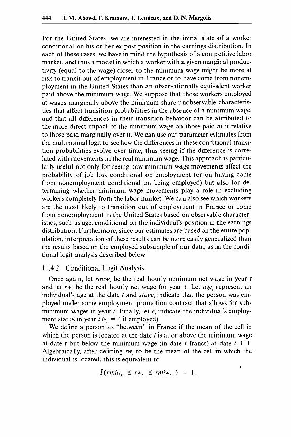
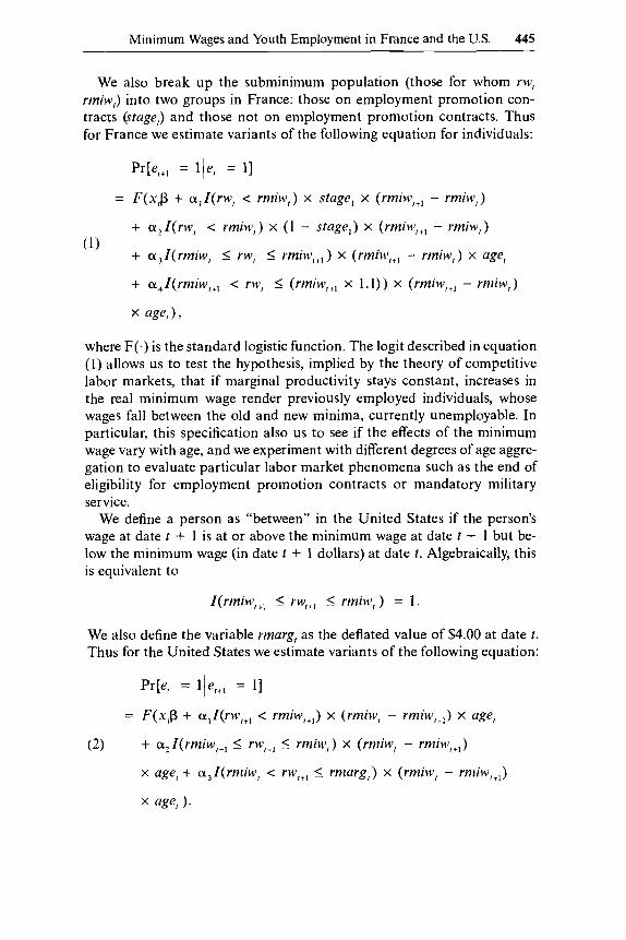
market between 1962 and 1972 with a high school diploma, and figure 1 1.13 shows the variation of the conditional transition probabilities for an American woman with the same characteristics.
Clearly, in the United States, the effect of age on the transition probabil- ities differs dramatically from the French case. The two figures are similar in form, although the relative reduction in the conditional probability of transitioning from nonemployed to marginally over the minimum is stronger for men and turns back up sooner for women. The most remark- able difference between the French and US. cases is that while in France the probability of making a 0 - N transition decreases with age, there is either no effect or a slight increase in the relative probability of N - 0 transi- tions (the U.S. equivalent) for older workers relative to younger workers

450 J. M. Abowd, F. Kramarz, T. Lemieux, and D. N. Margolis
in our results for the United States. This could be due to the high stability in general of jobs that pay substantially over the minimum wage; the inter- cepts for E-0 transitions are significantly larger than all other estimated intercepts in the model. On the other hand, in the United States it seems that the probability of transitioning from nonemployment to marginally over the minimum wage is the transition the most affected by aging, while in France the order of magnitude of the change is about half for 31-40- year-olds relative to 16-18-year-olds (a 63 percent drop vs. a 27 percent drop for men, a 39 percent drop vs. a 24 percent drop for women). If workers paid marginally over the minimum are indeed a reasonable con- trol group for minimum wage workers, the relatively feeble decline in the probability of having come from nonemployment experienced by workers paid at the minimum suggests that in the United States at least, the mini- mum wage is playing a role in determining the sorts of transitions that low-wage workers make in the labor market.
11.6 Conditional Logit Results
1 1.6.1 France
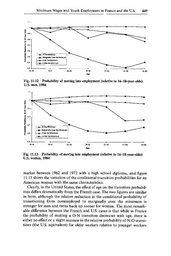
Table 11.3 shows the results of estimating equation (1) for France on young people, using broad age categories.I0 We have reported the coeffi- cients for the key real minimum wage variables, as well as variables for several types of employment contracts in France.I’
The coefficients show that French men aged 25-30 with real wage rates in period t that are above the real minimum in t but below the real mini- mum wage in period t + 1 have much lower subsequent employment prob- abilities than similar men paid substantially over the period t + 1 real minimum wage. The elasticity is very large: an increase of 1 percent in the minimum wage entails an decrease in the probability of keeping one’s job of 4.6 percent, relative to men aged 25-30 who are paid marginally over the minimum. One interpretation of these results is that although low- wage workers do differ from high-wage workers (as the fairly consistent negative coefficients suggest), the minimum wage hits workers whose real wages are between the two minima much harder than other low-wage workers.
Similar results hold for women and people 20-24 years old, but these coefficients are less significant. In general, the employment loss effects worsen with age among the young employed population, but the level of
10. Appendix table 11A.4 provides descriptive statistics for the French data used in these regressions.
11. We explicitly consider fixed-term contracts (CDD), youth employment schemes (young stagidre), and apprenticeships, with the reference being long-term contracts (CDI). See Ab- owd, Corbel, and Kramarz (1999) for more detail on the differences between CDD and CDI.
Table 11.3 Estimated Effect of Real French Minimum Wage Increases on Subsequent Employment Probabilities: Broad Age Categories
Standard Name of Effect Coefficient Error p-Value Elasticity
Young Men, Hourly Wage
Fixed-term contract Young stugiuire Apprentice Real wage, < Real SMIC, and Not young stugiuirr Redl wage, < Real SMIC, and Young stugiuire (Real SMIC, 5 Real wage, 5 Real SMIC,,,)*(16 5 Age, 5 19) (Real SMIC, c Real wage, c Real SMIC,+,)*(ZO 5 Age, 5 24) (Real SMIC, C Real wage, 5 Real SMIC,,,)*(25 5 Age, 5 30) (Real SMIC,,, C Real wage, 5 (I.l*Real SMIC,,,))*(16 5 Age, d 19) (Real SMIC,,, 5 Real wage, 5 (I.l*Real SMIC,+,))*(ZO 5 Age, c 24) (Real SMIC,,, 5 Real wage, 5 (I.l*Real SMIC,,,))*(25 c Age, c 30)
-.5129 -.8777 -.I490 2.9500 9.0935 5.4614
-7.7651 - 33.2708
2.9869 -3.41 1 1 -3.7791
,0819 .I263 ,1364
2.3341 5.5130 8,5478 8.2247 9.9755 5.2162 4.2892 5.87 I3
.OOOl
.0001 ,2741 ,1867 ,0990 ,5229 ,3451 ,0009 ,5669 ,4264 ,5198
- ,0478 -.0818 -.0139
,7765 5.4727 2.0094
- 1.2017 -4.8928
1.1201 - .4256 -.2914
Fixed-term contract Young stugiuirr Apprentice Real wage, < Real SMIC, and Not young srugkire Real wage, < Real SMIC, and Young srugiuire (Real SMIC, 5 Real wage, 5 Real SMIC,,,)*(16 c Age, c 19) (Real SMIC, 5 Real wage, 5 Real SMIC,+,)*(20 C Age, C 24) (Real SMIC, 5 Redl wage, 5 Real SMIC,,,)*(25 5 Age, 5 30) (Real SMIC,,, 5 Real wage, 5 (l.I*Real SMIC,+,))*(16 5 Age, c 19) (Real SMIC,,, 5 Real wage, 5 (I.l*Real SMIC,+,))*(ZO c Age, c 24) (Real SMIC,,, 5 Real wage, C (l.I*Real SMIC,+,))*(25 c Age, 5 30)
-.9351 -1.4152 - 1.0683 -.8857 8.3441
-1.6553 -8.7397 - 11.6779 - 5. I875
,3164 - 1.6632
,0826 .I150 ,1954
2.3804 5.0400 9.8606 6.81 85 7.8799 7.6851 4.4018 4.7962
.0001
.0001
.0001 ,7098 ,0978 ,8667 ,1999 ,1383 ,4997 ,9421 ,7288
Young Women, Hourly Wage
-.0879 -.I331 -.I005 -.I604 4.4279 -.2759 - 1.2485 -1.5537 - ,7447
.0354 -.I734
Source: French Labor Force Survey, 1982-89, matched year to year.
Note: Equations estimated by maximum likelihood logit. All equations include indicators for year, education (eight groups), region (Ile de France), and age (three groups), as well as the continuous variables labor force experience (through quartic), seniority, seniority squared, and hourly wage in year I (through cubic). All displayed coefficients except fixed- term contract, young sfugiuire, and apprentice are equal to the indicated group multiplied by the real percentage increase in the SMIC between years t and t + I (1981 = 100). The coefficients and elasticities show the partial effects on the probability of employment in year t + I . given t . A separate equation was estimated for each demographic panel. Sample sizes are young men, 30,804; young women, 26,434.

452 J. M. Abowd, F. Kramarz, T. Lemieux, and D. N. Margolis
detail is not sufficient to speculate on why certain age groups are more affected than others. It is clear from the estimates of the coefficients on the different contract types that all of the types of contract studied here lead to more precarious labor force attachment than an indefinite term contract on average, but the employment promotion contracts (young stagiuire) seem to provide relative security for the subminimum popula- tion.” Looking at these populations in more detail, in particular at what happens to 25-year-olds (who will no longer be eligible for employment promotion contracts the following year), will give us more information on whether the dramatic differences seen between 25-30-year-old and 20-24- year-old men with wages between the two minima are due to the expira- tion of the protection provided by the employment promotion contracts. Table 11.4 gives these detailed results.
Looking first at the men, the most remarkable feature is in fact the huge negative coefficient affecting 25-year-old men whose wages are between the two minima. This elasticity of - 15.9 (expressed as a difference from the marginally above category) and the subsequent negative coefficients for “between” men are consistent with the idea that the minimum wage has a strong negative impact on subsequent employment probabilities. However, the presence of employment promotion contracts, and the re- duction in employer social insurance contributions that they imply, helps workers who are under age 25 to retain their jobs in the face of a steadily increasing real SMIC. When workers are no longer eligible for such con- tracts, their probability of losing their jobs increases dramatically. Relative to the control group of workers marginally above the SMIC, the coeffi- cients for 25- and 26-year-olds are significantly larger. In fact, there is no significant bump in the coefficients at 25 years old for the marginally above workers, suggesting that this phenomenon is only pertinent to minimum wage workers. This further reinforces the interpretation that “between” workers who are eligible for employment promotion contracts are shielded from the negative effects of movements in the SMIC, but “older” young workers are not.
On average, the coefficients for workers between the two SMICs are more negative than for workers marginally over the date t SMIC. The av- erage difference (excluding the 25-year-olds) is 7.8, suggesting that the “be- tween” population might be different from the “marginal” population. Unfortunately, none of these differences (except for 25-year-olds) is sig- nificant, and in fact, none of the other coefficients for men are significantly different from zero. Although there are also a few significant coefficients in the results for women, interpretation of these results is much more dif- ficult. Although 23-year-old women with wages between the two minima
12. See Bonnal, Fougkre, and Serandon (1997) for an analysis centered on the impact of the youth employment schemes.
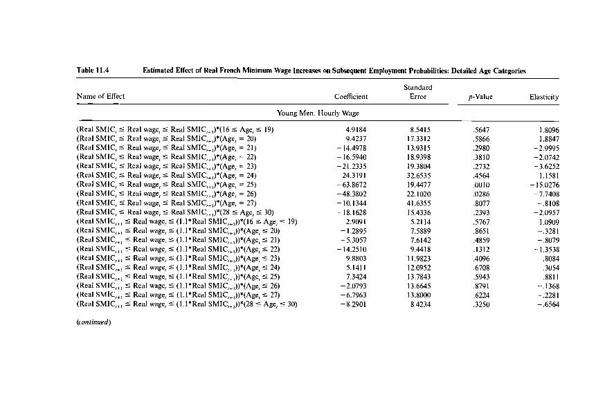
Table 11.4 Estimated Effect of Real French Minimum Wage Increases on Subsequent Employment Probabilities: Detailed Age Categories
Standard Name of Effect Coefficient Error p-Value Elasticity
Young Men, Hourly Wage
(Real SMIC, 5 Real wage, 5 Real SMIC,+,)*(16 5 Age, 5 19) (Real SMIC, 5 Real wage, 5 Real SMIC,+,)*(Age, = 20) (Real SMIC, I Real wage, 5 Real SMIC,+,)*(Age, = 21) (Real SMIC, 5 Real wage, 5 Real SMIC,+,)*(Age, = 22) (Real SMIC, 5 Real wage, 5 Real SMIC,+,)*(Age, = 23) (Real SMIC, 5 Real wage, I Real SMIC,+,)*(Age, = 24) (Real SMIC, I Real wage, 5 Real SMIC,+,)*(Age, = 25) (Real SMIC, 5 Real wage, I Real SMIC,+,)*(Age, = 26) (Real SMIC, 5 Real wage, 5 Real SMIC,+,)*(Age, = 27) (Real SMIC, 5 Real wage, 5 Real SMIC,+,)*(28 5 Age, 5 30) (Real SMIC,,, 5 Real wage, I (I.l*Real SMIC,+,))*(16 I Age, 5 19) (Real SMIC,,, 5 Real wage, 5 (].]*Real SMIC,+,))*(Age, 5 20) (Real SMIC,,, 5 Real wage, 5 (I.l*Real SMIC,+,))*(Age, 5 21) (Real SMIC,,, 5 Real wage, 5 (I.l*Real SMIC,+,))*(Age, 5 22) (Real SMIC,,, 5 Real wage, s (I.l*Real SMIC,+,))*(Age, 5 23) (Real SMIC,,, 5 Real wage, 5 (I.l*Real SMIC,+,))*(Age, 5 24) (Real SMIC,,, 5 Real wage, 5 (I.l*Real SMIC,+,))*(Age, 5 25) (Real SMIC,,, 5 Real wage, I (I.l*Real SMIC,+,))*(Age, 26) (Real SMIC,,, 5 Real wage, 5 (I.l*Real SMIC,+,))*(Age, 5 27) (Real SMIC,,, I Real wage, 5 (I.l*Real SMIC,+,))*(28 5 Age, 5 30)
(con I inued)
4.9 184 9.4237
- 14.4978 - 16.5940 -21.2335
24.3191 -63.8672 -48.3802 - 10.1344 - 18.1628
2.9091 - 1.2895 -5.3057
-14.2510 9.8803 5.1411 7.3424
-2.0793 -6.7963 - 8.2901
8.5415 17.33 I2 13.931 5 18.9398 19.3804 32.6535 19.4477 22.1020 41.6355 15.4336 5.21 14 7.5889 7.6142 9.4418
1 1.9823 12.0952 13.7843 13.6645 13.8000 8.4234
,5647 ,5866 ,2980 ,3810 ,2732 ,4564 .0010 ,0286 ,8077 .2393 S767 ,8651 ,4859 ,1312 ,4096 ,6708 ,5943 ,8791 ,6224 .3250
1.8096 1.8847
-2.9995 -2.0742 -3.6252
1.1581 - 15.0276
-7.7408 -.8108
-2.0957 1.0909
-.3281 - ,8079 - 1.3538
,8084 ,3054 ,881 1
-.I368 -.2281 -.6564

Table 11.4 (continued)
Name of Effect Standard
Coefficient Error p-Value Elasticity
Young Women, Hourly Wage
(Real SMIC, 5 Real wage, 5 Real SMIC,+,)*(16 5 Age, 5 19)
(Real SMIC, 5 Real wage, 5 Real SMIC,+,)*(Age, = 21) (Real SMIC, S Real wage, s Real SMIC,+,)*(Age, = 22)
(Real SMIC, 5 Real wage, 5 Real SMIC,+,)*(Age, = 24)
(Real SMIC, 5 Real wage, s Real SMIC,+,)*(Age, = 26)
(Real SMIC, 5 Real wage, 5 Real SMIC,+,)*(28 5 Age, (Real SMIC,,, 5 Real wage, 5 (I.l*Real SMIC,+,))*(16 5 Age, S 19)
- 1.7276 (Real SMIC, 5 Real wage, 5 Real SMIC,+,)*(Age, = 20) 38.9118
-2.5471 - 14.8695 - 35.7959 -26.8 167
(Real SMIC, 5 Real wage, 5 Real SMIC,+,)*(Age, = 23)
(Real SMIC, 5 Real wage, Real SMIC,+,)*(Age, = 25) 4.9443
(Real SMIC, 5 Real wage, 5 Real SMIC,+,)*(Age, = 27) -17.3310
.3354 - 18.7008
-5.2027 30)
(Real SMIC,,, 5 Real wage, (I.l*Real SMIC,+,))*(Age, S 20) 26.3323 (Real SMIC,,, 5 Real wage, s (I.l*Real SMIC,+,))*(Age, 5 21) 7.0573 (Real SMIC,,, 5 Real wage, 5 (I.l*Real SMIC,+,))*(Age, 5 22) (Real SMIC,,, 5 Real wage, 5 (I.l*Real SMIC,+,))*(Age, 5 23) (Real SMIC,,, 5 Real wage, 5 (I.l*Real SMIC,+,))*(Age, 5 24) (Real SMIC,,, 5 Real wage, 5 (I.l*Real SMIC,+,))*(Age, 5 25)
- 14.9729 -4.4278 -6.0435 - ,0432
(Real SMIC,,, 5 Real wage, 5 (I.l*Real SMIC,+,))*(Age, 5 26) (Real SMIC,,, 5 Real wage, 5 (l.I*Real SMIC,+,))*(Age, 5 27)
1.5230 7.7465
(Real SMIC,,, 5 Real wage, 5 (I.l*Real SMIC,+,))*(28 5 Age, 30) -7.2571
9.8645 23.1330 12.7138 14.21 27 14.0221 17.8484 23.7480 15.5787 18.9002 1 1.4752 7.6973
11.6838 8.8323 8.3171 9.8576 9.7212
10.5009 9.9692
1 2.224 I 7.0661
3610 ,0926 ,8412 ,2955 .O I07 .I330 ,8351 ,2659 ,9858 ,1032 ,4991 ,0242 ,4243 .07 18 ,6533 ,5341 ,9967 ,8786 S263 ,3044
-.2879 3.0882 -.3069
-2.2876 -7.8100 -4.3098
,5494 -2.3788
.0419 -2.6715 - ,7469 2.7296
,7876 - 1.7468 - . SO09 - .6784 - ,0054
,1488 ,7173
- ,7392
Source: French Labor Force Survey, 1982-89, matched year to year. Nore: Equations estimated by maximum likelihood logit. All equations include indicators for year, education (eight groups), region (Ile de France), and age (ten groups), fixed-term contract, young stugiuire, apprentice, paid under the SMIC and young stugiuire, and paid under the SMIC and not young stugiuire, as well as the continuous variables labor force experience (through quartic), seniority, seniority squared, and hourly wage in year t (through cubic). All displayed coefficients are equal to the indicated group multiplied by the real percentage increase in the SMIC between years 1 and f + l (1981 = 100). The coefficients and elasticities show the partial effects on the probability of employment in year I + I , given employment in year 1. Sample sizes are young men, 30,804; young women, 26,434.

Minimum Wages and Youth Employment in France and the U.S. 455
are significantly more likely to be nonemployed the following year than women who are paid over the SMIC, the difference from 23-year-old women paid marginally over the SMIC is not significant. And the large, positive coefficients on 20-year-old women, again present in both the “be- tween” and “marginal” populations, is hard to explain. These results may reflect the added opportunities available for women as men go off to per- form their military service (and thus withdraw from the labor market), but such an interpretation can neither be accepted not rejected exclusively on the basis of the evidence presented here.
In addition to estimating the conditional logits with “marginally over” the SMIC defined as 1.10 times the SMIC, we also estimated these models with two alternative definitions (1.15 and 1.20 times the SMIC). Table 1 1.5 analyzes the robustness of the coefficients for the between and marginal categories to these changes in the definition of “marginally over.” It seems clear that our results are quite robust to changes in the definition of “mar- ginal .”
1 1.6.2 United States
Table 1 I .6 shows the results of estimating equation (2) using both the hourly wage measure that excludes income from tips and the measure that
Table 11.5 Robustness of Conditional Logit Results to Variations in Definition of “Marginally over” the Minimum
~
Narrow Medium Wide
Marginally Marginally Marginally Between Over Between Over Between Over
French youth Men 4.0888
Women -6.0281 (6.6196)
(8.2804) U.S. youth
Men 1.9965
Women 3.9599 (1.6373)
(1.5578)
,7317 (3.8171) -.04525 (4.2333)
- 1.6196 (1.8837)
(1.8022) -.8667
5.3906 (6.6543)
(8.3 134)
2.0827 (1.7436) 4.6514
(1.6694)
-6.0108
4.0222 (2.6087) -.4013 (3.1828)
- 1.9342 (1.7077) -.5443 (1.661 5 )
6.5107 (6.7083)
-5.8400 (8.3 809)
1.5043 (1.7871) 3.8852
(1.7297)
5.0473 (2.4817) -.I178 (3.0601)
-2.6988 (1.6751) - 1.6244
( I .6484)
Sources: French Labor Force Survey, 1982-89, matched year to year, and U.S. Current Population Survey, 1981-87, January-May and September-December, matched year to year. Note: Coefficients come from logistic regressions conditional on employment at date t for France and date f + I for the United States. For France, the categories are defined as “narrow” = SMIC to I.lO*SMIC, “Medium” = SMIC to 1.15*SMIC, and “wide” = SMIC to I.20*SMIC. For the United States, the categories are defined as “narrow” = $3.35 to $3.75, “medium” = $3.35 to $4.00, and “wide” = $3.35 to $4.25. For this table, “youth” is defined as ages 25 and under. See notes to tables 11.3, 11.4, 11.6, 1 1.7, and 1 1.8 for details on other variables in the regressions. Numbers in parentheses are standard errors.
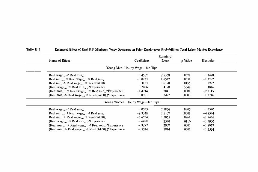
Table 11.6 Estimated Effect of Real US. Minimum Wage Decreases on Prior Employment Probabilities: Total Labor Market Experience
Name of Effect Standard
Coefficient Error p-Value Elasticity
Young Men, Hourly Wage-No Tips
Real wage,+,< Real min,,, - ,4567 2.5368 ,8571 -.I498 Real rnin,,, 5 Real wage,,, 5 Real min, - 3.0723 1.6532 ,063 1 - 1.3287 Real min, 5 Real wage,,, 5 Real ($4.00), ,3153 1.6178 .8455 ,0977 (Real wage,,, 5 Real min,,,)*Experience ,2406 ,4178 ,5648 ,4046 (Real min,,, 5 Real wage,,, 5 Real min,)*Experience -1.4714 ,2841 .ooo 1 -2.5115 (Real min, 5 Real wage,,, 5 Real ($4.00),)*Experience -.8961 ,2497 ,0003 - 1.3746
Young Women, Hourly Wage-No Tips
Real wage,,,< Real rnin,,, -.0535 2.1856 ,9805 - ,0340 Real rnin,,, 5 Real wage,,, 5 Real min, -8.3538 1.5107 ,000 I -4.8544 Real min, 5 Real wage,,, 5 Real ($4.00), -2.6704 1.5055 ,076 I - 1.8436 (Real wage,,, 5 Real min,,,)*Experience - ,6488 ,2570 .01 I6 - 1.3900 (Real min,,, 5 Real wage,,, 5 Real min,)*Experience - ,9277 .2007 .ooo I - 1.8917 (Real min, 5 Real wage,,, 5 Real ($4.00),)*Experience - ,8574 .I894 .ooo 1 - 1.5564

Young Men, Hourly Wage-With Tips
Real wage,+,< Real rnin,,, -2.6088 2.4905 .2949 - 1.7404 Real rnin,,, 5 Real wage,,, I Real min, -4.3814 1.6346 ,0074 -2.4823 Real min, 5 Real wage,,, I Real ($4.00), -.7521 1.6034 ,6390 -.5111
(Real min, 5 Real wage,,, I Real ($4,00),)*Experience - ,9464 ,249 1 .ooo 1 - 1.4794
(Real wage,,, 5 Real min,,,)*Experience ,1059 .4 154 ,7988 ,1805 (Real min,,, 5 Real wage,,, 5 Real min,)*Experience - 1.5673 ,2849 ,000 1 -2.6350
Young Women, Hourly Wage-With Tips
Real wage,+,< Real rnin,,, -3.0938 2.0570 ,1326 - 1.8775 Real rnin,,, I Real wage,,, 5 Real min, -9.1702 1.4879 ,000 1 -5.2774 Real min, I Real wage,,, 5 Real ($4.00), - 3.3 I96 1.4939 ,0263 -2.2658 (Real wage,,, I Real min,,,)*Experience -.7841 2570 .0023 - 1.7565 (Real rnin,,, 5 Real wage,,, 5 Real min,)*Experience - ,9762 .2009 ,000 1 - 1.9923 (Real min, 5 Real wage,,, 5 Real ($4.00),)*Experience - ,885 1 ,1894 .ooo 1 -1.6186
Source: Current Population Survey, 1981-87, January-May and September-December, matched year to year. Note: Equations estimated by maximum likelihood logit. All equations include indicators for year, region (three groups), nonwhite, and married; and years of schooling, labor force experience (through quartic), and log hourly real wage (I982 prices, through cubic). All displayed coefficients are equal to the indicated group times the real decrease (absolute value of the change in logarithms) in the minimum wage between years t and t+ 1 . The coefficients and elasticities show the partial effects on the probability of employment in year f , given employment in year t+ I . A separate equation was estimated for each panel. Sample sizes are young men, 41,001; young women, 38,992.

458 J. M. Abowd, F. Kramarz, T. Lemieux, and D. N. Margolis
includes income from tips, and interacting with total labor market experi- ence instead of age.I3 In every case, individuals who are employed in year t + 1 were more likely to have been unemployed or not in the labor force in t if their real wage in t + 1 was between the real minimum wage in years t and t + 1. The magnitudes of these effects are large, with elasticities for men with zero experience of - 1.42 to - 1.97 and for women with no experience of -3.01. Once again, we refer to comparisons with the “mar- ginal’’ group-that is, workers who are paid marginally above the old (date t ) minimum wage-to get at the direct effect of movements in the real minimum wage on transitions into employment. By weighting the different experience groups, a decrease in the real minimum wage of 1 percent between t - 1 and t is related to an increased probability of having been nonemployed at t - 1 of 2.2 percent (in difference from the marginal workers) for those men who are paid between the t and t + 1 minimum wages. These results are consistent with the neoclassical idea that de- creases in the real minimum wage make nonemployed workers easier to employ and these workers enter disproportionately between the two mini- mum wages. This decreases the share of those employed at date t + 1 who were employed at date t for the “between” group more than for other groups.
It is interesting to note the differences, or rather lack of differences, between the results that measure wages with and without tips. None of the qualitative results seem sensitive to the manner in which we define wages; however, some intuition can be gleaned from how the coefficients seem to shift when passing from measures without tips to measures with tips. All of the coefficients shown in table 1 1.6 become more negative when tips are included in the wage measure. This is also consistent with the standard neoclassical model, which would imply that the measure with tips more accurately describes a worker’s marginal productivity and would conclude that the less significant coefficients in the estimation without tips are affected by measurement error. Nevertheless, due to the lack of any qualitative difference between the results with and without tips, and be- cause our measure without tips uses reported rather than constructed data,I4 the rest of our results for the United States will be based on the wage measure that excludes tips.
Table 11.7 reestimates equation (2) using the broad age categories, as in table 1 1.3. As was suggested by the negative coefficients on the experience interaction terms in table 1 1.6, the effects of the minimum wage worsen as young workers get older. The differences between workers paid between the two minima and workers paid marginally over the t minimum are still
13. Appendix table 1 IA.5 provides descriptive statistics for the U.S. data used in these re-
14. Welch (1997) provides evidence on various sorts of measurement error in the CPS and gressions.
hints that hours are likely to be a greater source of measurement error than wages.

Table 11.7 Estimated Effect of Real US. Minimum Wage increases on Prior Employment Probabilities (excluding tips): Broad Age Categories
Name of Effect Standard
Coefficient Error p-Value Elasticity ~~ ~ ~
Young Men, Hourly Wage
Real wage,+,< Real rnin,,, ,6119 1.9147 ,7493 ,2007 (Real rnin,,, 5 Real wage,,, 5 Real min,)*(16 5 Age, 5 19) -6.1455 1.3807 ,000 1 -2.9233 (Real min,,, 5 Real wage,,, 5 Real min,)*(20 5 Age, 5 24) - 1 1.8902 1.9536 .0001 - 4.209 5 (Real rnin,,, Real wage,,, 5 Real min,)*(25 5 Age, 5 30) -19.4188 3.1495 .OOOl -5.9588 (Real min, 5 Real wage,,, Real ($4.00),)*(16 Age, 5 19) - ,9696 1.3901 .4855 -.3767 (Real min, 5 Real wage,,, 5 Real ($4.00),)*(20 5 Age, s 24) -5.9107 1.7693 .0008 - 1.4697 (Real min, 5 Real wage,,, 5 Real ($4.00),)*(25 S Age, 5 30) -9.8243 2.4330 .0001 - 1.8055
~~
Young Women, Hourly Wage
Real wage,,,< Real rnin,,, -3.2195 1.6924 ,0571 -1.1762 (Real min,,, 5 Real wage,,, 5 Real min,)*(16 5 Age, 5 19) -9.1433 1.3730 ,000 1 -4.3346 (Real rnin,,, 5 Real wage,,, 5 Real min,)*(20 5 Age, 5 24) -14.0812 1.6615 ,000 I -4.8644 (Real rnin,,, 5 Real wage,,, 5 Real min,)*(25 5 Age, 5 30) -19.8125 1.8812 ,000 1 -7.1220 (Real min, 5 Real wage,,, 5 Real ($4.00),)*(16 Age, 5 19) -3.0577 1.4261 ,0320 -1.1732 (Real min, 5 Real wage,,, 5 Real ($4.00),)*(20 5 Age, 5 24) -8.4481 1.4157 ,000 I -2.2399 (Real min, 5 Real wage,,, 5 Real ($4.00),)*(25 5 Age, 5 30) - 12.5349 1.5423 .0001 -3.2334
Source: Current Population Survey, 1981-87, January-May and September-December, matched year to year. Note: Equations estimated by maximum likelihood logit. All equations include indicators for year, region (three groups), nonwhite, married, and age (three groups); and years of schooling, labor force experience (through quartic), and log hourly real wage (1982 prices, through cubic). All displayed coefficients are equal to the indicated group times the real decrease (absolute value of the change in logarithms) in the minimum wage between years t and t+ 1. The coefficients and elasticities show the partial effects on the probability of employment in year f, given employment in year t + l . A separate equation was estimated for each demographic panel. Sample sizes are young men, 41,001; young women, 38,992.
460 J. M. Abowd, F. Kramarz, T. Lemieux, and D. N. Margolis
significant for all age groups, and the elasticities are still large. For the oldest age group, a decrease of 1 percent in the real minimum wage at t is associated with a 5.96 percent higher chance that a given “between” worker came from nonemployment, whereas such a change is associated with only an 1.81 percent higher chance for “marginal” workers. Unlike the French case, although 25-30-year-olds with date t + 1 wages between the two minima have a higher chance of having come from nonemploy- ment than do 20-24-year-olds, the difference is not nearly as dramatic. This is not surprising, as there existed no nationwide employment promo- tion schemes in the United States in the 1980s that would have induced effects similar to the French case.
One might think that our approach of considering previous employment in the United States could be subject to the possibility, especially among young people, that many of the transitions from nonemployment to em- ployment are first jobs after the end of s~hool ing . ’~ Since we control for schooling as a set of regressors reflecting different levels of educational attainment, looking at the pattern of age coefficients for “between” work- ers and “marginal” workers should allow us to ignore such considerations to the extent that entry into the labor force does not occur disproportion- ately in a particular wage category. Table 1 1.8, which provides our condi- tional logit analysis at the same level of aggregation as table 1 1.4, therefore allows us to concentrate more precisely on how minimum wage move- ments affect the stability of early career employment at different points in the wage distribution.
As was the case in our earlier results, the probability that a worker came from nonemployment is higher among the set of workers with date t + 1 real wages between the two minima than among the set of workers with date t + 1 real wages marginally above the date t real minimum. The same holds true for a comparison of “between” workers with workers earning substantially more than the date t real minimum, and these differences are often significant. Despite a lot of variation across the different ages, there appears to be a secular trend toward a higher and higher share of workers coming from nonemployment as age increases, and this trend is steeper among “between” workers than among “marginal” workers, particularly for young men. This is not the case in France, and it may suggest that information is revealed faster in the United States and that as workers age, the sorts of low-wage jobs they can find become increasingly precarious.
Since there do not exist systematic, targeted programs that should affect transitions among young people throughout the United States in the same manner (with the exception of education), interpretation of these coeffi- cients is not as straightforward as in the French case. However, if (as men-
15. See Topel and Ward (1992), among others, for an analysis of early career mobility in the United States.
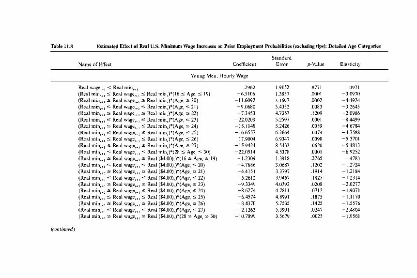
Table 11.8 Estimated Effect of Real US. Minimum Wage Increases on Prior Employment Probabilities (excluding tips): Detailed Age Categories
Name of Effect Standard
Coefficient Error p-Value Elasticity
Young Men, Hourly Wage
Real wage,,, < Real rnin,,, (Real rnin,,, 5 Real wage,,, I Real min,)*(16 5 Age, I 19) (Real min,,, 5 Real wage,,, 5 Real min,)*(Age, 5 20) (Real rnin,,, 5 Real wage,,, 5 Real min,)*(Age, 5 21) (Real rnin,,, 5 Real wage,,, 5 Real min,)*(Age, 5 22) (Real rnin,,, 5 Real wage,,, 5 Real min,)*(Age, 5 23) (Real rnin,,, I Real wage,,, 5 Real min,)*(Age, 5 24) (Real rnin,,, 5 Real wage,,, 5 Real min,)*(Age, 5 25) (Real rnin,,, 5 Real wage,,, 5 Real min,)*(Age, 5 26) (Real rnin,,, 5 Real wage,,, 5 Real min,)*(Age, 4 27) (Real rnin,,, 5 Real wage,,, 5 Real min,)*(28 5 Age, 5 30) (Real rnin,,, I Real wage,,, I Real ($4.00),)*(16 5 Age, 4 19) (Real rnin,,, I Real wage,,, 5 Real ($4.00),)*(Age, 5 20) (Real rnin,,, 5 Real wage,,, 5 Real ($4.00),)*(Age, 5 21) (Real min,,, 5 Real wage,,, 5 Real ($4.00),)*(Age, 5 22) (Real rnin,,, 5 Real wage,,, 5 Real ($4.00),)*(Age, 5 23) (Real rnin,,, 5 Real wage,,, 5 Real ($4.00),)*(Age, 5 24) (Real rnin,,, 5 Real wage,,, 5 Real ($4.00),)*(Age, 5 25) (Real rnin,,, I Real wage,,, 5 Real ($4.00),)*(Age, 5 26) (Real rnin,,, 5 Real wage,,, 5 Real ($4.00),)*(Age, 5 27) (Real min,,, 5 Real wage,,, 5 Real ($4.00),)*(28 5 Age, 5 30)
,2962 -6.5106 - 1 1.6092 -9.0680 -7.3453 - 22.0209 -15.1148 - 16.6557 - 17.9004 - 15.9424 -22.05 I4 - 1.2309 -4.7686 -4.4151 -5.2612 - 9.3349 -8.6274 -6.4574 -8.4370 - 12. I263 - 10.7899
1.9152 1.3857 3.1697 3.4352 4.7357 5.2597 5.2426 6.2664 6.9347 8.5432 4.5378 1.3918 3.0687 3.3797 3.9467 4.0392 4.781 I 4.8991 5.7535 5.3991 3.5679
,8771 .ooo 1 .0002 .0083 . I209 ,000 I ,0039 ,0079 ,0098 ,0620 ,000 I .3765 ,1202 ,1914 ,1825 ,0208 .07 I2 ,1875 ,1425 .0247 .0025
,0971 -3.0970 -4.4924 -3.2645 -2.0986 -8.4499 -4.6784 -4.7588 -5.3701 -5.1813 -6.9252 - ,4783 - 1.2724 -1.2184 -1.2314 -2.0277 -1.9071 -1.1170 - 1.5576 -2.4804 - 1.9561
(continued)

Table 11.8 (continued)
Name of Effect Standard
Coefficient Error p-Value Elasticity
Young Women, Hourly Wage
Real wage,,, < Real min,,, -3.7559 1.6913 .0264 - 1.3722 (Real rnin,,, 5 Real wage,,, 5 Real min,)*(16 5 Age, c 19) -9.8220 1.3730 .0001 -4.6564 (Real rnin,,, 5 Real wage,,, 5 Real min,)*(Age, 5 20) - 12.2205 2.8456 .0001 -4.6320 (Real rnin,,, 5 Real wage,,, 5 Real min,)*(Age, 5 21) - 12.8276 3.1 141 .0001 -4.6853 (Real min,,, 5 Real wage,,, 5 Real min,)*(Age, 5 22) - 13.4058 3.6339 .0002 -4.4009 (Real rnin,,, 5 Real wage,,, 5 Real min,)*(Age, 5 23) -14.131 I 4.2524 .0009 -4.1771 (Real rnin,,, 5 Real wage,,, 5 Real min,)*(Age, c 24) - 14.0301 4.2585 .oo I0 -4.1895 (Real min,+, 5 Real wage,,, 5 Real min,)*(Age, 5 25) -23.5188 4.2544 ,000 I -9.5817 (Real rnin,,, 4 Real wage,,, 5 Real min,)*(Age, 5 26) - 18.8257 4.0242 ,000 I -6.4372 (Real rnin,,, 5 Real wage,,, 5 Real min,)*(Age, I 27) -20.1282 4.6770 ,000 I -6.8814 (Real rnin,,, 5 Real wage,,, 5 Real min,)*(28 5 Age, 5 30) - 19.6787 2.4999 ,000 1 -6.9948 (Real rnin,,, 5 Real wage,,, 5 Real ($4.00),)*(16 5 Age, 5 19) -3.4490 1.4233 .O 154 - 1.3234 (Real rnin,,, 5 Real wage,,, 5 Real ($4.00),)*(Age, 5 20) -2.3108 2.8808 ,4225 - ,5968
(Real rnin,,, 5 Real wage,,, 5 Real ($4.00),)*(Age, 5 22) -9.1566 3.0945 ,003 1 -2.5897 (Real rnin,,, 5 Real wage,,, 5 Real ($4.00),)*(Age, 5 23) - 13.4398 3.2502 ,000 1 -3.4858 (Real rnin,,, 5 Real wage,,, 5 Real ($4.00),)*(Age, 5 24) - 14. I707 3.4026 .0001 -3.7468 (Real rnin,,, 5 Real wage,,, 5 Real ($4.00),)*(Age, 5 25) - 16.7514 3.1826 .0001 -4.7081 (Real rnin,,, 5 Real wage,,, 5 Real ($4.00),)*(Age, I 26) -7.2195 3.7185 .0522 - 1.5576 (Real rnin,,, 5 Real wage,,, 5 Real ($4.00),)*(Age, 5 27) -6.5597 3.5805 .0669 - 1.4072 (Real rnin,,, 5 Real wage,,, 5 Real ($4.00),)*(28 S Age, 5 30) - 15.0802 2.0915 ,000 I -4.2146
(Real rnin,,, 5 Real wage,,, 5 Real ($4.00),)*(Age, 5 21) -4.9630 2.93 I8 ,0905 - 1.3019
Source: Current Population Survey, 1981-87, January-May and September-December, matched year to year. Note: Equations estimated by maximum likelihood logit. All equations include indicators for year, region (three groups), nonwhite, married, and age (ten groups); and years of schooling, labor force experience (through quartic), and log hourly real wage (1982 prices, through cubic). All displayed coefficients are equal to the indicated group times the real decrease (absolute value of the change in logarithms) in the minimum wage between years t and t + 1. The coefficients and elasticities show the partial effects on the probability of employment in year t , given employment in year t + 1. A separate equation was estimated for each demographic panel. Sample sizes are young men, 41,001; young women, 38,992.

Minimum Wages and Youth Employment in France and the U.S. 463
tioned above) the coefficients corresponding to a given age are particularly strong, and if this age corresponds to the age at which many students typically finish a certain diploma, one might conclude that the coefficients are capturing disproportionate entry into the labor force at particular places in the wage distribution. Unfortunately, the most remarkable co- efficients (23 years old for men and 25 years old for women) are not con- current with ages at which a significant portion of the future workforce is in their last year of schooling. There does not seem to be any clear inter- pretation for the particular age pattern of the coefficients in the United States.
Finally, to promote comparability between our analysis, which is done conditional on the employment state in either year t (France) or year t + 1 (United States), and other analyses, which consider the effects of the mini- mum wage unconditional on the previous or future employment state, we compute the implied unconditional elasticities implied by our estimates. To calculate an unconditional elasticity we apply Bayes law to obtain the relation between the forms of the analysis equations we used for France and the United States. Hence, we have
Pr[e,+, = lie, = l,rmiw,,rmiw,tl]
To calculate the elasticity we use the following derivative formula:
Notice that the derivative in equation (4) simplifies because the denomina- tor in the ratio of unconditional probabilities in equation (3) does not depend on the future minimum wage. The right-hand side of equation (4) has two terms. For France, we can estimate only the first of these two terms because the real minimum wage is always increasing. The conditions necessary for estimating the second term occur in the United States, where the real minimum wage is always decreasing. To estimate the uncondi- tional elasticity in equation (4) we must make an assumption regarding the term that cannot be estimated in the particular country. We assume that this term is zero, which means that increases in the real minimum wage do not change the rate at which nonemployed workers become em- ployed and, conversely, decreases in the real minimum wage do not change
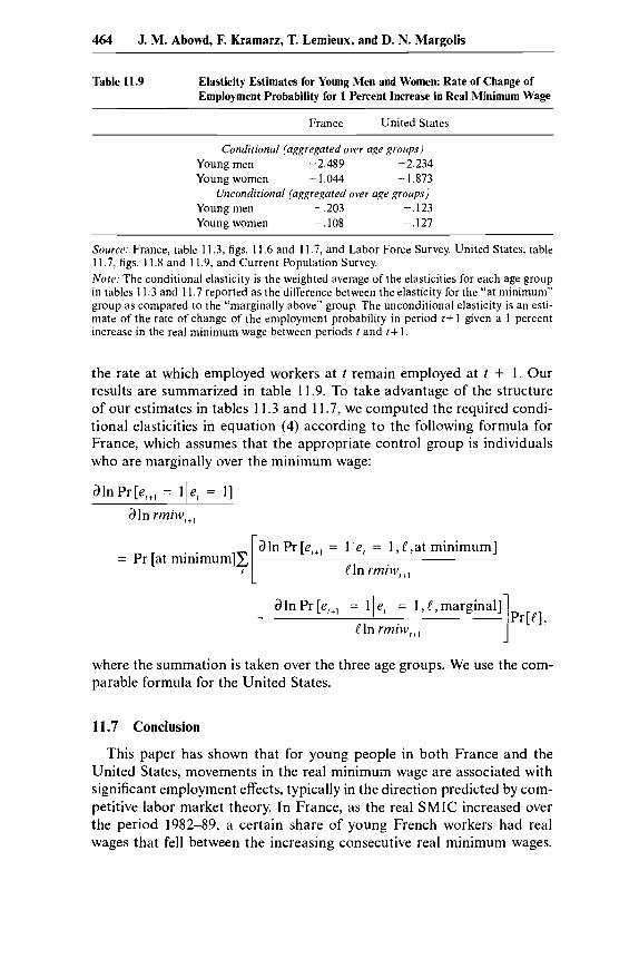
464 J. M. Abowd, F. Kramarz, T. Lemieux, and D. N. Margolis
Table 11.9 Elasticity Estimates for Young Men and Women: Rate of Change of Employment Probability for 1 Percent Increase in Real Minimum Wage
France United States
Conditional (aggregated over uge groups) Young men -2.489 -2.234 Young women - 1.044 -1.873
Young men - ,203 -.123 Young women -.I08 -.I27
Unconditional (aggregated over age groups)
Source; France, table 1 1.3, figs. 1 I .6 and 1 1.7, and Labor Force Survey. United States, table 1 1.7, figs. 1 1.8 and 11.9, and Current Population Survey. Note: The conditional elasticity is the weighted average of the elasticities for each age group in tables 11.3 and 11.7 reported as the difference between the elasticity for the “at minimum” group as compared to the “marginally above” group. The unconditional elasticity is an esti- mate of the rate of change of the employment probability in period t+ 1 given a 1 percent increase in the real minimum wage between periods t and t+ 1.
the rate at which employed workers at t remain employed at t + 1. Our results are summarized in table 11.9. To take advantage of the structure of our estimates in tables 1 1.3 and 1 1.7, we computed the required condi- tional elasticities in equation (4) according to the following formula for France, which assumes that the appropriate control group is individuals who are marginally over the minimum wage:
alnPr[e,,, = lie, = 11
alnPr[e,,, = lie, = l,e,atminimum]
!In rmiw,,, = Pr [at minimum]^
Pr[Pl, 1 aInPr[e,,, = lie, = l , ~ , m a r g i n a ~ ]
Pln rmiw,,, -
where the summation is taken over the three age groups. We use the com- parable formula for the United States.
1 1.7 Conclusion
This paper has shown that for young people in both France and the United States, movements in the real minimum wage are associated with significant employment effects, typically in the direction predicted by com- petitive labor market theory. In France, as the real SMIC increased over the period 1982-89, a certain share of young French workers had real wages that fell between the increasing consecutive real minimum wages.

Minimum Wages and Youth Employment in France and the US. 465
For workers in this situation, subsequent employment probabilities fell significantly. However, participation in employment promotion programs seemed to shield these workers from some of the effects of the increasing real SMIC, and when this eligibility ended, the probability of subsequent nonemployment shot up dramatically. In the United States, a comparable effect of a real minimum wage moving in the opposite direction occurred, as many workers had market wage rates that were passed by the declining real minimum wage over the period 1981-87. American workers whose current real wage rate would have been below the real minimum wage in earlier periods were much less likely to have been employed in those ear- lier periods.
By comparing effects of minimum wage movements on workers em- ployed at the minimum with the effects on those employed marginally above it, we identify the direct effects of the minimum wage, as distinct from heterogeneity across the wage distribution in labor force attachment and response to macroeconomic shocks. We suppose that these workers have identical labor supply behavior, but they also have much higher sub- sequent reemployment probabilities in France as well as much higher prior employment probabilities in the United States. Within the youth popula- tion, these strong effects increase with age in the United States, and the pattern in France is dominated by eligibility for employment promotion contracts. Across the population as whole, however, our multinomial logit results suggest that in both countries, it is youths who are most affected by movements in the real minimum wage.
Even if the conditional elasticities in question are large, the at-risk groups (workers between two minimum wages) are relatively small-8 per- cent of young men and 10 percent of young women in France, 6 percent of young men and 7 percent of young women in the United States. Thus overall unconditional elasticities tend to be much lower than the elasticit- ies conditional on being between the two minima. If the relevant policy question concerns the impact of the minimum wage on those individuals most likely to be affected by it (i.e., those currently paid at the minimum wage), our results suggest that there are much larger negative employment effects on this group, especially as compared to the group in the wage distribution marginally above the minimum, than other research has found.

Appendix
Table l l A . l Statistical History of the Salaire Minimum Interprofessionnel de Croissance (SMIC)
Gross Employee Employer Net Monthly Total Payroll Payroll
Statutory Hourly Real Hourly Monthly Monthly Compensation Tax Rate Tax Rate Consumer Hours per SMIC SMIC (1970) SMIC SMIC cos t ('YO at ((%I at Price Index
Year Month (francs) (francs) (francs) (francs) (francs) SMIC) SMIC) (1970 = 100)
1951 1952 1953 1954 1955 1956 1957 1958 1959 1960 1961 I962 1963 1964 1965 1966 1967 1968 1969
173.3 173.3 173.3 173.3 173.3 173.3 173.3 173.3 173.3 173.3 173.3 173.3 173.3 173.3 173.3 173.3 173.3 173.3 173.3
0.89 1 .oo 1 .oo 1.15 1.25 1.26 I .29 1.46 1.58 1.61 1.64 1.72 1.84 1.89 1.97 2.06 2.13 2.68 3.16
1.95 1.96 1.98 2.29 2.46 2.43 2.42 2.39 2.43 2.39 2.36 2.36 2.41 2.39 2.43 2.48 2.49 3.00 3.32
154.41 173.33 173.33 199.98 216.45 218.40 223.78 253.87 270.62 279.19 284.69 298.77 319.62 328.27 342.28 358.27 368.32 484.81 548.16
145.15 162.93 182.33 187.98 203.46 205.30 210.35 238.64 253.84 261.88 267.04 278.45 297.09 305.13 318.15 331.15 339.66 426.84 503.32
195.78 220.74 222.47 256.67 277.81 280.32 287.22 319.50 349.51 360.57 370.52 393.33 418.88 430.20 448.56 468.00 498.45 617.17 728.07
6.00 6.00 6.00 6.00 6.00 6.00 6.00 6.00 6.20 6.20 6.20 7.05 7.05 7.05 7.05 7.05 8.15 8.17 8.18
26.79 21.35 28.35 28.35 28.35 28.35 28.35 28.85 29.15 29.15 30.15 3 1.65 31.05 31.05 31.05 31.36 35.33 32.78 32.82
45.60 50.98 50.39 50.21 50.80 5 1.80 53.21 61.19 64.98 67.40 69.59 72.9 I 76.38 78.98 80.98 83.22 85.41 89.28 95.12

1970 1971 1972 1973 1974 1975 1976 1977 1978 1979 1980 1981 1982 1983 1984 1985 1986 1987 1988 1989 1990 1991 1992 1993 1994
173.3 173.3 173.3 173.3 173.3 173.3 173.3 173.3 173.3 173.3 173.3 173.3 169.0 169.0 169.0 169.0 169.0 169.0 169.0 169.0 169.0 169.0 169.0 169.0 169.0
3.42 3.76 4.19 4.95 6.10 7.26 8.34 9.40
10.61 11.94 13.80 16.30 19.17 21 S O 23.53 25.44 26.53 27.60 28.65 29.54 30.80 32.30 33.58 34.45 35.20
3.42 3.56 3.74 4.12 4.46 4.75 4.98 5.13 5.31 5.40 5.49 5.72 6.02 6.16 6.27 6.41 6.51 6.56 6.64 6.60 6.66 6.77 6.87 6.9 1 6.92
59 1.92 65 I .72 725.96 858.27
1,053.74 1,260.25 1,466.01 1,629.59 1,839.61 2,068.69 2,391.67 2,824.41 3,323.46 3,725.87 4,077.88 4,335.00 4,482.87 4,663.84 4,79 1.7 1 4,991.42 5,205.20 5,458.70 5,674.46 5,821.21 5,947.96
543.50 598.15 668.00 786.52 967.78
I , I 50.86 1,306. I8 1,464.19 1,650.68 1,817.14 2,085.54 2,478.98 2,892.07 3,216.92 3,465.79 3,676.51 3,177.27 3,894.77 3,977.60 4,093.46 4,269.83 4,547.95 4,606.38 4,794.70 4,881.38
786.13 867.31 971.62
1,151.28 I ,42 1.63 1,71 1.87 1.98 1.47 2,239.06 2,536.45 2,843.62 3,324.42 3,925.93 4,623.60 5,221.43 5,693.33 6,056.88 6,270.64 6,528.91 6,715.10 6,943.58 7,182.1 3 7,527.66 7,860.94 7,945.37 7,98 I .57
8.18 8.22 8.26 8.36 8.42 8.68 9.67
10.15 10.27 12.14 12.80 12.23 12.98 13.66 15.01 15.19 15.74 16.49 16.99 17.99 17.97 17.39 17.98 18.38 18.64
32.81 33.08 33.84 34. I4 34.53 35.82 37.03 37.40 37.88 38.91 39.00 39.00 39.12 40.14 39.62 39.72 39.88 39.99 40.14 39.1 1 37.89 37.90 38.53 36.49 34.19
100.00 105.52 I 1 1.99 120.20 136.71 152.80 167.49 183.22 199.82 221.30 25 1.30 285.00 318.70 349.29 375.19 397.04 407.62 420.43 43 1.74 447.33 462.38 477.20 488.60 498.86 508.84
Source: Friez and Julhes (1998). Note: Data for 1950-69 are for the earlier minimum wage system (suhire minimum interprofessionnel guruntie).
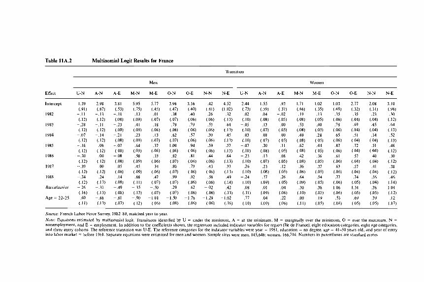
Table l lA.2 Multinomial Logit Results for France
Transition
Men Women
Effect U-N A-N A-E M-N M-E 0 - N 0 - E N-N N-E U-N A-N A-E M-N M-E 0 - N 0 - E N-N N-E
Intercept
1982
1983
I984
1985
1986
1987
1988
Eacculuuriur
Age = 22-25
1.39 -2.98 -3.81 (.91) (37) (33 )
- . I 1 - . I3 - . I 8 (.12) (.12) (.08)
-.28 - . I 1 -.23 (.12) (.12) (.OX)
-.07 -.I4 -.21 (.I21 (.12) (.08)
-.I6 .06 -.07 (.12) (.I2) (.OX)
-.30 .OO -.08 (.I2) (.I2) (.OX)
-.39 .MI .os (.12) (.12) (.08)
-.34 .24 .I4 (.I2) (.13) (.08)
(.16) (.13) (.OX) .60 -.68 -21 (.)I) (.13) (.07)
-.26 - . 31 -.49
-.42 -4.52 (.41) (1.02) .26 .32
(.06) (.13) .53 .64
(.06) (.13) .30 .45
(.06) (.13) .s9 .57
(.06) (.13) .44 .64
(.06) (.13) .43 .33
(.06) (.13) .S6 .49
(.06) (.14)
(.06) (.13)
(.06) (.16)
-.02 .42
-1.29 -1.02
Source: French Labor Force Survey, 1982-89. matched year to year.
Note: Equations estimated by multinomial logit. Transitions identified by U = under the minimum, A = at the minimum, M = marginally over the minimum, 0 = over the minimum, N =
nonemployment, and E = employment. In addition to the coefficients shown, the regression included indicator variables for region (Ile de France), eight education categories, eight age categories. and three entry cohorts. The reference transition was U-E. The reference categories for the indicator variables were year = 1981, education = no degree. age = 41-50 years old, and year of entry into labor market = before 1961. Separate equations were estimated for men and women. Sample sizes were men, 145,646; women, 166,716. Numbers in parentheses are standard errors.

Table 11 A.3 Multinomial Logit Results for the United States
Transition
Men Women
Effect N-U N-A E-A N-M E-M N - 0 E - 0 N-N E-N N-U N-A E-A N-M E-M N - 0 E - 0 N-N E-N
Intercept -1.61 . I I .30 .SO 1.20 4.28 6.60 - 3 0 -.39 - 4 9 2.74 .81 3.45 1.94 5.56 6.91 .34 1.40 (1.06) (36) ( S 8 ) (.91) (34) (SI) (.44) (.44) (.46) (.67) (37) (.40) (.61) (.38) (.42) (.32) (.32) (.34)
19x2 .04 . I7 .02 . I 3 .I0 .26 .07 .I6 .06 .06 .09 .04 .09 - .02 . I4 .09 .06 .02 (.07) (.OS) (.04) (.06) (.04) (.04) (.04) (.04) (.04) ( .OS) (.04) (.03) (.04) (.03) (.03) (.03) (.03) (.03)
1983 ~ .07 .22 .OO . I8 .0S .34 .09 . IS - .05 .OO . I3 .OO .07 -.06 .17 . I I .OS - .01 (.08) (.05) (.04) (.06) (.04) (.04) (.04) (.04) (.04) (.OS) (.04) (.03) (.04) C.03) (.03) (.03) (.03) (.03)
1984 .O I .22 .OS .20 .08 .30 . I6 .20 .03 .01 . I6 - .06 . I2 - .01 .24 .I9 .I0 .OS (.09) (.06) (.06) (.07) (.05) (.05) (.OS) (.OS) (.OS) (.06) (.04) (.04) ( .OS) (.04) (.04) (.03) (.03) (.03)
(.12) (.OX) (.07) (.09) (.07) (.07) (.06) (.06) (.06) (.08) (.06) ( .OS) (.06) (.05) (.05) (.04) (.04) (.04)
(.OX) (.OS) (.OS) (.06) (.OS) (.05) (.04) (.04) (.04) (.05) (.04) (.03) (.04) (.03) C.03) (.03) (.03) (.03)
(.09) (.07) (.OS) (.07) (.OS) (.OS) (.04) (.04) (.04) (.06) (.OS) (.04) (.06) (.04) (.04) (.03) (.03) (.03)
(.27) (.21) (.14) (.22) (.13) (.12) ( . I I ) ( . I I ) ( . I I ) (.16) (.I)) (.lo) (.14) (.09) (.lo) (.OX) (.OX) (.08)
1985 .01 . I6 .02 .22 .I7 .34 .27 .27 .06 - .08 . I I -_ 12 .21 - .04 .26 .22 .06 .02
1986 -.06 .09 -.OX .20 .06 .35 .20 .21 .OS -.05 .09 -.07 .I6 -.06 .36 .29 .I0 .OX
High school -.I2 .I3 .OX .I6 .I2 .49 .7S .I2 .38 -.I4 .OS -.02 .I9 .20 .37 .6S -.05 .22
Age = 22-25 .09 . I 3 .I0 .2S .I4 .20 - . I 1 -36 -.71 . I3 .63 .21 .76 .2S .S2 .21 -.64 -.21
Source: Current Population Survey, 1981-87. January-May and September-December, matched year to year. Nule: Equations estimated by multinomial logit. Transitions identified by U = under the minimum, A = at the minimum, M = marginally over the minimum, 0 = over the minimum, N = nonemployment, and E = employment. I n addition to the coefficients shown, the regression included indicator variables for six education categories, eight age categories, and three entry cohorts. The reference transition was E-U. The reference categories for the indicator variables were year = 19x1, education = no diploma, age = 61 years old or older, and year of entry into labor market = before 1961. Separate equations were estimated for men and women. Sample sizes were men, 162,073; women, 199,682. Numbers in parentheses are standard errors.

Table l l A . 4 Descriptive Statistics Conditional on Employment: France
Entire Population Youth
Men Women Men Women
Indicator Mean S.D. Mean S.D. Mean S.D. Mean S.D.
Age Seniority Experience Fixed-term contract Apprentice Youth slugiuire Paris region Year = 1988 Year = 1987 Year = 1986 Year = 1985 Year = 1984 Year = 1983 Year = 1982 No education Elementary school Junior high school Basic vocationalltechnical Advanced vocationaVtechnical school Bucculuur6ut (high school) Technical college or university Grad school or postcollege professional school Employed next period? Observations under SMIC and Sfugiaire Observations under SMIC and Not sfugiuire Observations between two real SMlCs Observations marginally over SMIC Total observations
37.5769 10.9995 20.5879
,0144 ,0064 ,0037 .2031 ,0692 ,1386 ,1374 ,1413 ,1437 .I455 . I479 ,2407 . I845 ,0610 ,2997 ,0509 ,0434 ,0495 ,0639 ,9285
329 5,548
849 4,146
104,081
10.7732 9.0239
14.7257 .I191 ,0795 .0611 ,4023 ,2538 ,3455 ,3443 ,3484 ,3508 .3526 .3550 ,4275 ,3879 ,2394 ,4581 .2199 ,2038 ,2169 ,2445 ,2577
36.9156 9.5347
19.6161 .0178 ,0021 ,0057 ,2350 ,0724 ,1444 . I420 ,1430 . I399 ,1411 ,1443 ,1821 ,2114 ,0920 ,2344 ,0689 ,0709 ,0841 ,0541 ,9209
422 9,826 1,292 5,44 I
80,993
10.9116 8.1790
13. I948 ,1322 ,0462 .0750 ,4240 .2592 ,3515 .3490 ,3501 ,3469 ,3481 ,3514 ,3859 ,4083 ,2890 ,4236 ,2533 ,2566 ,2776 ,2263 ,2699
25.0472 4.2628 7.5144
.0342
.02 I6 ,0124 ,1907 ,0641 ,1343 ,1342 ,1385 .I427 ,1481 ,1554 ,2361 .0978 .0794 ,3989 ,0477 ,0460 ,0554 ,0387 ,9068
329 3,256
494 2,155
30,804
3.6006 5.7013
12.0523 ,1697 ,067 I ,0818 ,3924 ,2449 ,3410 ,3409 ,3453 ,3498 ,3552 ,3623
1.4579 ,2941 ,2701 .4896 .2103 ,2050 .2 I57 ,1727 ,2666
24.9998 3.4430 4.4259 6.1117 6.8722 10.8535
.0357 . I756
.0065 ,0389
.0173 ,0986 ,2217 ,4151 ,0629 ,2428 .I 349 ,341 5 .I352 ,3419 ,1401 ,3471 . I402 ,3471 ,1490 ,3561 ,1567 ,3635 ,1635 1.5493 .0963 .2908 .I055 .3072 ,3129 .4632 .OM7 ,2831 ,0921 ,2878 ,1008 ,2891 ,0401 ,1815 .9060 ,2871
424 3,617
645 2,206
26,434
Source: French Labor Force Survey, 1982-89, matched year to year.
Nofe: S.D. = standard deviation. “Youth is defined as ages 30 and under.

Table l l A . 5 Descriptive Statistics Conditional on Employment: United States ~~ ~~
Entire Population Youth
Men Women Men Women
Indicator Mean S.D. Mean S.D. Mean S.D. Mean S.D.
Years of education Experience Nonwhite Married Year = 1981 Year = 1982 Year = 1983 Year = 1984 Year = 1985 Northeastern region North-central region Southern region Employed previous period? Observations under minimum wage Observations between two real minimum wages Observations marginally over minimum wage Total observations
12.8629 20.5188
.I156 ,7055 .2005 .2004 ,2049 ,1133 ,0706 ,2326 .26 18 ,3215 ,9170 2,571 4,085 6,799
121,356
2.8842 12.9620
,3198 ,4558 ,4004 ,4003 ,4036 ,3169 ,2561 ,4225 ,4396 ,4670 ,2760
12.8531 20. I023
,1399 ,5973 ,1937 .2000 ,2023 ,1151 ,0721 .2316 ,2613 ,3249 ,8705 5,367 7,645
13,218 110,287
2.4770 12.9669
.3469
.4905
.3952 ,4000 ,4017 ,3191 ,2587 .42 19 ,4393 ,4683 ,3358
12.7341 7.3809
.1177 ,4366 .2048 ,2007 .2076 ,1137 ,0694 ,2249 ,2679 ,3251 ,8397 1,475 3,177 4,664
41,001
2.2514 4.0105
,3223 ,4960 .4035 .4005 ,4056 ,3174 ,2542 ,4175 ,4429 ,4684 ,3668
12.9628 6.9846
.I312 4342 .20 I9 .2061 ,2043 ,1138 ,0695 .2304 ,2684 .3 176 .7977 2,48 I 4,434 6,097
38,993
2.0845 3.9707
,3376 ,4957 .40 I4 ,4045 ,4032 ,3176 ,2542 ,421 1 ,443 1 ,4655 ,4017
Source: Current Population Survey, 1981-87, January-May and September-December, matched year to year. Note: S.D. = standard deviation. “Youth” is defined as ages 30 and under.

472 J. M. Abowd, F. Kramarz, T. Lemieux, and D. N. Margolis
References
Abowd, John M., Patrick Corbel, and Francis Kramarz. 1999. The entry and exit of workers and the growth of employment: An analysis of French establish- ments. Review of Economics and Statistics 81 (May): 170-87.
Abowd, John M., Francis Kramarz, and David N. Margolis. 1999. High wage workers and high wage firms. Econometrica 67 (March): 251-333.
Bayet, Alain. 1994. Les salaires de 1991 a 1993 dans le secteur prive et semi-public. INSEE Resultats, no. 64. Paris: Institut National de la Statistique et des Etudes Economiques.
Bazen, S., and J. F! Martin. 1991. L’impact du salaire minimum sur les salaires et I’emploi en 1994. Note du Bureau Emploi-Salaires no. 95BD4.
Bonnal, Liliane, Denis Fougere, and Anne Serandon. 1997. Evaluating the impact of French employment policies on individual labour market histories. Economic Studies 64:683-7 13.
Brown, Charles, C. Gilroy, and A. Kohen. 1982. The effect of the minimum wage on employment and unemployment. Journal of Economic Literature 20 (June): 487-528.
Dolado, Juan, Francis Kramarz, Steven Machin, Alan Manning, David Margolis, and Coen Teulings. 1996. The economic impact of minimum wages in Europe. Economic Policy 23 (October): 319-72.
Friez, Adrien, and Mathieu Julhes. 1998. SCries longues sur les salaires, edition 1998. INSEE Rtsultats, no. 605. Paris: Institut National de la Statistique et des Etudes Economiques.
Hsiao, Cheng. 1986. The analysis of panel data. Cambridge: Cambridge Univer- sity Press.
Linneman, Peter. 1982. The economic impacts of minimum wage laws: A new look at an old question. Journal of Political Economy 90 (June): 443-69.
Margolis, David. 1993. Compensation practices and government policies in Western European labor markets. Ph.D. diss., Cornell University, Ithaca, N.Y.
Neumark, David, and William Wascher. 1992. Employment effects of minimum and subminimum wages: Panel data on state minimum wage laws. Industrial and Labor Relations Review 46 (October): 55-81.
Topel, Robert H., and Michael P. Ward. 1992. Job mobility and the careers of young men. Quarterly Journal of Economics 107 (May): 439-79.
Welch, Finis. 1997. Wages and participation. Journal of Labor Economics 15 (Janu- ary): S77-S103.