minimum variance time of arrival estimation for positioning

ARTICLE IN PRESS

Contents lists available at ScienceDirect

Signal Processing

Signal Processing 90 (2010) 2611–2620

0165-16

doi:10.1

� Cor

munica

1-3 (Ca

E-m

(J. Serra

journal homepage: www.elsevier.com/locate/sigpro

Fast communication

Minimum variance time of arrival estimation for positioning

Luis Blanco a, Jordi Serra a, Montse Najar a,b,�

a Centre Tecnol�ogic de Telecomunicacions de Catalunya (CTTC), Parc Mediterrani de la Tecnologia (PMT), Av. Canal Olımpic S/N,

08860 Castelldefels, Barcelona, Spainb Department of Signal Theory and Communications, Universitat Polit�ecnica de Catalunya (UPC), Jordi Girona, 1-3 (Campus Nord–M �odul D5),

08034 Barcelona, Spain

a r t i c l e i n f o

Article history:

Received 6 August 2009

Received in revised form

28 January 2010

Accepted 11 February 2010Available online 20 February 2010

Keywords:

TOA

Minimum variance

Wireless location

84/$ - see front matter & 2010 Elsevier B.V. A

016/j.sigpro.2010.02.018

responding author at: Department of Signal

tions, Universitat Polit�ecnica de Catalunya (

mpus Nord–M �odul D5), 08034 Barcelona, Spa

ail addresses: [email protected] (L. Blanco), jord

), [email protected] (M. Najar).

a b s t r a c t

Positioning systems based on time of arrival (TOA) rely on an accurate estimation of the

first signal arrival which is the only one bearing position information. In this context,

first arrival path detectors based on the minimum variance (MV) and the normalized

minimum variance (NMV) criteria are robust against multipath propagation and non-

line-of-sight (NLOS) situations. The aim of the paper is twofold. On the one hand,

efficient implementations of those criteria will be presented. On the other hand, two

polynomial rooting procedures based on the MV criterion will be exposed. As it will be

shown, they lead to better performance than the traditional MV versions based on a grid

search. In general, these methods imply finding the roots of a polynomial with complex

coefficients. In order to reduce their computational burden a conformal mapping is

proposed herein.

& 2010 Elsevier B.V. All rights reserved.

1. Introduction

Location systems based on TOA require an accurateestimation of the first time-delay. Unfortunately, inwireless channels, multipath propagation and non-line-of-sight (NLOS) situations bias the estimation of the firstsignal arrival. In this context, detectors based on themaximum of the impulse response [1], despite theirlow computational burden, are not suitable becausethe delayed replicas displace the maximum of theresponse. Analogously, conventional correlators cannotseparate the direct path from the echoes if they are closeor the direct propagation path is highly attenuated [2]. Onthe other hand, conventional parametric methods basedon the maximum likelihood (ML) criteria provide a

ll rights reserved.

Theory and Com-

UPC), Jordi Girona,

in.

[email protected]

complete channel description at expenses of a heavycomputational burden, leading to an expensive multi-dimensional search (e. g. [3–5]).

As it is well-known, time delay estimation in thefrequency domain and spectral (or spatial) analysis areclosely connected [6]. In this context, high resolutionspectral techniques such as multiple signal classification(MUSIC) and root-MUSIC can be used as TOA estimators[2,7–9]. These methods are commonly referred in theliterature as subspace or singular value decomposition(SVD) methods and are based on the separation of thesignal and the noise subspaces. This characterization iscostly and needs the knowledge of the number ofpropagation paths. Another well-known SVD techniquewhich avoids the traditional scanning of MUSIC is totalleast squares estimation of signal parameters via rota-tional invariance technique (TLS-ESPRIT) and it wasapplied to time delay estimation in [10]. Bearing in mindthe analogy between time delay estimation and spectralanalysis, high resolution methods based on the minimumvariance (MV) [11] and on the normalized minimum

www.elsevier.com/locate/sigpro

dx.doi.org/10.1016/j.sigpro.2010.02.018

mailto:[email protected]





ARTICLE IN PRESS

L. Blanco et al. / Signal Processing 90 (2010) 2611–26202612

variance (NMV) [12] criteria were successfully developedand applied to location systems in [13,14]. Thesetechniques can provide an accurate estimation of the firstsignal arrival at an affordable cost in high multipathenvironments, even when the line of sight (LOS) signal isstrongly attenuated. Herein, efficient implementations ofthe grid search of the MV and NMV TOA estimators basedon fast Fourier transform (FFT) are described, allowing asignificant reduction on the computational burden [22].Furthermore, new polynomial approaches which trans-form the grid search of the MV into a polynomial rootingprocedure are exposed in this paper. The first of thesetechniques is obtained deriving the MV power delayprofile (PDP) and it is referred herein as root derivativeminimum variance (RDMV). This method is closely relatedto the second polynomial algorithm, the root minimumvariance (RMV) estimator which was briefly introduced in[15] and later on analyzed in detail in [16] in the contextof angle of arrival (AOA) estimation. The performance ofthe RMV algorithm as a TOA estimator in a locationsystem is explored in this paper yielding accurate results,even better than those of the NMV estimator, at least formoderate or low SNR. In order to reduce the computa-tional cost of the rooting techniques a conformal trans-formation [17] is described herein. This mappingcircumvents the complex nature of the polynomialstransforming them into a polynomial with real coeffi-cients. As efficient rooting procedures based on realarithmetic are applicable, a significant reduction on thecomputational burden can be achieved without accuracyreduction. A similar approach was applied to MUSIC in thecontext of AOA estimation in [18].

The main goal of this paper is to analyze theperformance of several TOA estimators based on theminimum variance criterion. The integration of partialresults presented by the authors in previous works in ageneral framework provides a more meaningful view ofthese techniques. To compare the performance of thesetechniques with a theoretical bound, the expression ofthe Cramer-Rao bound is derived herein. It is based on thefrequency domain signal model of the received signal andit leads to a simple and compact expression.

The paper is organized as follows. In Section 2 thesignal model is described. The different TOA algorithmsare derived in Section 3. Performance analysis of thesemethods and simulation results in a realistic mobilescenario are shown in Section 4. Finally, concludingremarks are addressed in Section 5.

2. Signal model

Let us consider N observations of a received signalconsisting of L superimposed delayed replicas of a knownwaveform gðtÞ embedded in noise:

yðt;nÞ ¼XL�1

i ¼ 0

aiðnÞgðt�tiÞþZðt;nÞ n¼ 1, . . . ,N ð1Þ

being aiðnÞ and ti the complex time-varying amplitudeand the time-delay of the i-th arrival, respectively.Without loss of generality let us assume

t0ot1o � � �otL�1. The additive white Gaussian noise isdenoted by Zðt;nÞ.In the frequency domain the expression (1) is transformedinto a weighted sum of complex exponentials embeddedin noise:

Yðo;nÞ ¼XL�1

i ¼ 0

aiðnÞGðoÞe�jotiþNðo;nÞ ð2Þ

where Yðo;nÞ is the noisy frequency domain observedsignal, GðoÞ denotes the Fourier transform of gðtÞ andNðo;nÞ is the additive noise in the frequency domain.Sampling (2) at om ¼o0m for m¼ 0,1, . . . ,M�1 ando0 ¼ 2p=M and rearranging the frequency domain sam-ples Yðm;nÞ into the vector yn 2 C

M�1 yields,

yn ¼GEhðnÞþgðnÞ ð3Þ

where the matrix G 2 CM�M is a diagonal matrix whosecomponents are the frequency samples GðomÞ and thematrix E¼ ½et0

et1� � � etL�1

� 2 CM�L contains the delay-signature vectors associated to each arriving delayedsignal, with eti

¼ ½1 e�jo0ti � � � e�jo0ðM�1Þti �T . The channelfading coefficients are arranged in the vectorhðnÞ ¼ ½h0 � � � hL�1�

T 2 CL�1, and the noise samples invector gðnÞ 2 CM�1.

3. MV TOA estimation

TOA can be estimated as the first delay that exceeds agiven threshold in the power delay profile, defined as thesignal distribution of the power with respect to propaga-tion delays. The PDP can be obtained by estimating thepower of the signal filtered at each delay [19],PðtÞ ¼wHðtÞRywðtÞ, where Ry is the correlation matrix ofthe received signal estimated from a collection of N

observations within the coherence time of the delays andð�Þ

Hdenotes the conjugate transpose operator. The vectorwðtÞ can be obtained by applying the minimum variancecriterion which consists of the minimization of the outputpower with the constraint wðtÞHGet ¼ 1, which guaran-tees that the signal is not distorted at the explored timedelay. This constrained minimization yields to a closed-form for the MV PDP estimation:

PMV ðtÞ ¼1

eHt GHR�1

y Getð4Þ

In the traditional approach, the value of the PDP isevaluated in a grid of time delays. Nevertheless, as theauthors described in [20,21], the expression (4) can bereformulated as a discrete Fourier transform (DFT) andefficiently implemented using a FFT of length P, where P isthe number of grid points,

PMV ðtÞ ¼1PM�1

k ¼ �Mþ1 DðkÞe�jo0tkð5Þ

being DðkÞ ¼PM�k

n ¼ 1½W�n,nþk where ½W�i,j is the elementcorresponding to the i-th row and the j-th column of thematrix W¼GHR�1

y G. The inversion of the correlationmatrix can be avoided using the Gohberg–Semenculformula [19], being the computational burden of thewhole process OðM2þP log2 PÞ.

ARTICLE IN PRESS

L. Blanco et al. / Signal Processing 90 (2010) 2611–2620 2613

Unfortunately, in practice, the MV PDP is stronglydependent on the filter bandwidth, which, on its turn,depends on the explored time delay. Furthermore, thepresence of the pulse shape in the frequency domain Gcauses significant side lobes which can be misinterpretedas arrivals. In order to counteract both undesired effects,the expression (4) can be normalized by the equivalentnoise bandwidth yielding the NMV PDP estimator.

PNMV ðtÞ ¼PMV ðtÞ

wðtÞHwðtÞ¼

eHt GHR�1

y Get

eHt GHR�2

y Getð6Þ

In spectral and spatial analysis it is well-known that theNMV estimator [12] exhibits better resolution propertiesthan the MV method [19], and this behaviour is stillpreserved in a TOA estimation framework.

A fast implementation of the NMV PDP estimationbased on the FFT can be obtained [21] as follows:

PNMV ðtÞ ¼PM�1

k ¼ �Mþ1 DðkÞe�jo0tkPM�1k ¼ �Mþ1 GðkÞe�jo0tk

being

GðkÞ ¼XM�k

n ¼ 1

½U�n,nþk and U¼ GHR�2y G ð7Þ

The numerator of the expression (7) can be expressed as

2RXM�1

k ¼ 0

DðkÞe�jð2ptk=MÞ

( )�Dð0Þ

where Rf�g denotes the real part operator. Analogously,the denominator can be rewritten as

2RXM�1

k ¼ 0

GðkÞe�jð2ptk=MÞ

( )�Gð0Þ

Therefore, the computational burden can be dramaticallyreduced computing the NMV estimator as the sample bysample division of two P-points FFT, being P the numberof desired grid points. In this case, the implementationrequires the computation of two P-points FFT with acomputational burden OðP log2 PÞ and the sample bysample division of the two FFT.

Since the first time-delay is the only one which bearsposition information, in both spectral methods, MV andNMV TOA estimators, the first arrival is determined as thefirst maximum of the power delay profile above a giventhreshold level. Herein, the considered threshold is theone presented in [13] and it depends on the noise power.

3.1. Root methods

Alternative implementations of the MV TOA estimatorbased on finding the roots of a polynomial are presentedin this section.

3.1.1. Root derivative minimum variance (RDMV)

The maximization of the MV PDP to find the timedelays is equivalent to the minimization of the denomi-nator of (5). Thus, writing the denominator of (5) in termsof r¼ e�jo0t, the maxima of the MV PDP correspond tothe roots of the derivative of

PM�1k ¼ �Mþ1 DðkÞrk with

respect to t, given by the polynomial AðrÞ ¼P2M�2

k ¼ 0 akrk,where a2M�2�k ¼�a�k being ak ¼ ðk�Mþ1ÞDðk�Mþ1Þ for0rkr2M�2 and aM�1 ¼ 0 [21]. This class of polynomialsis called *-antisymmetric or *-antipalindromic, and thezeros either lie on the unit circle or appear in conjugatereciprocal pairs [23]. Note that now the timedelay information is wrapped in the phase of thezeros. Therefore, only the roots lying on the lowercomplex semi-plane have a clear physical meaning,because these are the only ones corresponding topositive delays.

3.1.2. Root minimum variance (RMV)

The second root approach consists of finding the rootsof the polynomial corresponding to the quadratic form ofthe denominator of the expression (5), BðrÞ ¼

P2M�2k ¼ 0 bkrk,

being bk ¼Dðk�Mþ1Þ for 0rkr2M�2 [24]. The hermi-tian property of W implies that bk ¼ b�2M�2�k, that is to say,they are conjugate symmetric, as a consequence, BðrÞbelongs to a class of polynomial named self-inversive or *-symmetric [23]. The roots of self-inversive polynomialseither lie on the unit circle or appear in conjugatereciprocal pairs. Nevertheless, a unit circle root wouldimply infinite power, and as a result the nulls of BðrÞalways appear in conjugate reciprocal pairs. Since half ofthe roots lie inside the unit circle and half outside, thepolynomial can be factored as BðrÞ ¼HðrÞH�ð1=rÞ, beingHðrÞ a FIR filter. Besides, there are efficient numericalalgorithms to compute HðrÞ [19]. Let us remark that onlythe nulls lying on the lower plane have clear physicalmeaning because they correspond to positive delays.Furthermore, the pairs of conjugate reciprocal roots wrapthe same time delay information. Therefore, only the rootslying inside the lower unit semicircle have to becomputed.As in the spectral methods, in the context of thepolynomial methods, RDMV and RMV, the comparisonwith a given threshold has to be considered. The firstarrival is determined as follows:

I.
Compute the roots of the corresponding polynomial. II. Extract the time-delay information wrapped in the
phase of the zeros. From Section 3.1.1, this relation isgiven by t¼�M=2p+r, where + denotes the phaseoperator.

III.
Evaluate the power of the estimated time-delay in theexpression (4).
IV.
Finally, pick the first meaningful delay as the first onecorresponding to a zero that exceeds the powerthreshold described in [13] for the MV method.
3.2. Conformal transformation

The root techniques imply finding the complex roots ofa polynomial with complex coefficients. In this context,conformal mapping, a powerful tool common in manyareas of physics and engineering [17], can be introduced.This kind of transformation circumvents the complexnature of the polynomial coefficients transforming theminto real ones.

ARTICLE IN PRESS

Real line

ω

rej�

α − jβ

α + jβ

Im{ }ρ

Re{ }ρ

}ρu {

u (−1) =1

u (1) = −1

1 ej�r

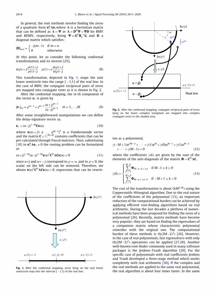
Fig. 2. After the conformal mapping, conjugate reciprocal pairs of zeros

lying on the lower complex semiplane are mapped into complex

conjugate zeros in the shaded area.


In general, the root methods involve finding the zerosof a quadratic form eH

t Ketwhere K is a hermitian matrixthat can be defined as K¼W or K¼DHWþWD for RMVand RDMV, respectively, being W¼ GHR�1

y G and D adiagonal matrix which satisfies:

½D�m,n ¼�jðm�1Þ if m¼ n

0 otherwise

�

At this point, let us consider the following conformaltransformation and its inverse [25],

uðrÞ ¼ jrðtÞþ j

rðtÞ�jrðtÞ ¼ j

uðrÞþ j

uðrÞ�jð8Þ

This transformation, depicted in Fig. 1, maps the unitlower semicircle into the range [�1,1] of the real line. Inthe case of RMV, the conjugate reciprocal pairs of zerosare mapped into conjugate roots as it is shown in Fig. 2.

After the conformal mapping, the m-th component ofthe vector et is given by

½et�m ¼ rm�1 ¼ jm�1 ðuþ jÞm�1

ðu�jÞm�1m¼ 1, . . . ,M ð9Þ

After some straightforward manipulations we can definethe delay-signature vector as,

et ¼ ðu�jÞ1�MCvðuÞ ð10Þ

where vðuÞ ¼ ½1 u . . . uM�1�T is a Vandermonde vectorand the matrix C 2 CM�M contains coefficients that can bepre-calculated through Pascal matrices. Then, substituting(10) in eH

t Ket ¼ 0 the rooting problem can be formulatedas

ðuþ jÞ1�Mðu�jÞ1�MvðuÞT CHKCvðuÞ ¼ 0 ð11Þ

since u= j and u=� j correspond to r¼1 and to r¼ 0, thescalar on the left side can be removed. Therefore, weobtain vðuÞT CHKCvðuÞ ¼ 0, expression that can be rewrit-

Im{ }ρ

Re{ }ρ

}ρu {

u (−1) =1u (1) =−1 u (−j) =0

Fig. 1. After the conformal mapping, zeros lying on the unit lower

semicircle map into the interval [�1,1] of the real line.

ten as a polynomial,

gð�Mþ1Þu2M�2þ � � � þgð1ÞuMþgð0ÞuM�1þgð1ÞuM�2

þ � � � þgðM�1Þ ¼ 0 ð12Þ

where the coefficients gðkÞ are given by the sum of theelements of the anti-diagonals of the matrix U¼ CHKC.

gðkÞ ¼

XM�k

n ¼ 1

UM�n�kþ1,n if M�1ZkZ0

XMþk

n ¼ 1

UM�nþ1,n�k if �Mþ1rko0

8>>>>><>>>>>:

ð13Þ

The cost of the transformation is about OðM2:38Þ using theCoppersmith–Winograd algorithm. Due to the real natureof the coefficients of the polynomial (13), an importantreduction of the computational burden can be achieved byapplying efficient root-finding algorithms based on realarithmetic. During the last decades a plethora of numer-ical methods have been proposed for finding the zeros of apolynomial [26]. Recently, matrix methods have becomevery popular; they are based on finding the eigenvalues ofa companion matrix whose characteristic polynomialcoincides with the original one. The computationalburden of these methods is Oðð2M�2Þ3Þ [26]. However,in the case of real polynomials, fast eigensolvers with onlyOðð2M�2Þ2Þ operations can be applied [27,28]. Anotherwell-known root-finder commonly used in many softwarepackages is the Jenkins–Traub algorithm [29]. For thespecific case of polynomials with real coefficients Jenkinsand Traub developed a three-stage method which workscompletely with real arithmetic [30]. If the complex andthe real methods are applied to the same real polynomial,the real algorithm is about four times faster. In the same

ARTICLE IN PRESS

4

5

6

7

8

rmse

[m]

rmse MVrmse NMVrmse RDMVrmse Root-MVCRB1/2


sense, another interesting method which only uses realarithmetic is the Bairstow’s algorithm [26]. It finds thequadratic factors corresponding with the conjugatepairs of zeros of the real polynomial. Herein matrixmethods are preferred because their robustness againstill-conditioned polynomial coefficients and their ability todiscriminate between clustered roots [26]. In Table 1 thecomputational burden of the algorithms described in thispaper is summarized.

0 10 20 30 40 50 60 700

1

2

3

SNR [dB]

Fig. 4. Performance of the TOA estimators in terms of RMSE in LOS

conditions and with a mean number of channel propagation paths equal

to 5.

10

4. Numerical results

In this section the performance of the TOA estimatorsintroduced in Section 3 will be assessed for differentchannel propagation conditions. First, let us introduce thesimulation environment that was used to obtain thenumerical results presented below. A mobile user tracingthe trajectory depicted in Fig. 3, relative to the basestations (BS) coordinates, is considered. The receivedsignal at the BS can be properly described by Eq. (1)where the waveform gðtÞ is a raised cosine with a roll-off

Table 1Summary of computational complexity of the exposed algorithms.

Method Computational complexity

MV OðM2þP log2 PÞ

NMV Sample by sample division of two P-

points FFT with a cost of OðP log2 PÞ each

one and OðM2Þ for the computation of

each covariance matrix inversion

RDMV and RMV without

conformal mappingOðð2M�2Þ3Þ using root-finding

algorithms based on matrix methods

RDMV and RMV with

conformal mappingOðð2M�2Þ2Þ using matrix methods and

about OðM2:38Þfor the conformal

transformation

-800 -700 -600 -500 -400 -300 -200-100 0 100 200-500

-400

-300

-200

-100

0

100

200

300

400

[m]

[m]

Base Station

Fig. 3. Trajectory that is considered to be traced by the mobile station in

the simulations related to TOA estimation performance.

0 10 20 30 40 50 60 700

1

2

3

4

5

6

7

8

9

SNR [dB]

rmse

[m]

rmse MVrmse RDMVrmse Root-MVCRB1/2

rmse NMV

Fig. 5. Performance of the TOA estimators in terms of RMSE in LOS

conditions and with a mean number of channel propagation paths equal

to 10.

0 10 20 30 40 50 60 700

5

10

15

20

25

SNR [dB]

rmse

[m]

rmse MVrmse NMVrmse RDMVrmse Root-MVCRB1/2

Fig. 6. Performance of the TOA estimators in terms of RMSE in NLOS

conditions.

ARTICLE IN PRESS


factor of 0.22. The number of rays at each trajectory point,L, is randomly generated according to a Poisson

iρ

iω

iωΔ

iρ ijrie ΦΔρi =

Z-Plane

Unit Circle

Re{ }ρ

Im{ρ}

Fig. 7. Effect of an error vector in the estimation of a signal root in the Z-

plane.

Fig. 8. Estimation of the MV, RMV and RDMV with SNR=30 dB. In the upper su

delays associated to the roots.

distribution, that is ProbðLÞ ¼ LLe�L=L!, where L is the

mean number of rays. The PDP is generated by using a oneside exponential decaying function, following the modelin [35], with realistic values of the delay spread generatedaccording to the statistical models described in [36]. Thepdf of the time delays is modelled accordingto a one side exponential decaying function, see [35].Considering the simulation environment described above,in Figs. 4 and 5 performance results for LOS conditionswith a mean number of channel rays equal to 5 and 10,respectively, are presented. In these figures, the root meansquare error (RMSE) is shown with respect to the SNR foreach method and it is compared with the square root ofthe CRB derived in the AppendixA, expression (14). It canbe observed that root methods (RDMV and RMV) offerbetter performance than MV based on grid search.Another important conclusion is that the RMV method isbetter than the NMV algorithm for the usual range of SNRin communications systems (lower than 15 dB) and,even for an asymptotic SNR, the RMV method offersapproximately the same performance than NMV. In Fig. 6,performance results of the TOA estimators in NLOSconditions are presented, the number of mean rays wasincreased to 15 and the first channel propagation pathwas attenuated a 50% in all the trajectory points. It is

bplot the zeros in the complex plane. In the lower one the PDP and the

ARTICLE IN PRESS


interesting to observe that root based methods (RMV andRDMV) are more robust to NLOS than MV based ongrid search. In order to see the performance advantageof the methods exposed in this paper with respect tosimpler methods that operate in the time domain, thesimulations of Figs. 4–6 were conducted for a maximumof the impulse response detector [1]. The results were asfollows, in LOS conditions, the RMSE was around 50 mfor a mean number of rays of 5 and 55 m for a meannumber of rays of 10. In NLOS conditions, the RMSEincreased to 70 m.

To get more insight in the performance of thealgorithms with respect to the SNR, let us studythe behaviour of the roots in the complex plane. InFig. 7 an error in the estimation of a signal root ri ¼ ejoi isrepresented by the vector Dri ¼ rie

jFi , then the estimatedroot can be defined as: r i ¼ ejoiþrie

jFi ¼ jr ijejo i . The error

vector in the complex plane can be decomposed into itsradial and angular components. Since the time delayinformation t is wrapped in the phase, the radialcomponent does not affect the delay estimation. Fig. 8represents the roots obtained with a three taps channel athigh SNR (30 dB). The upper plot represents the RMV andRDMV roots in the complex plane, in the lower plot thePDP and the time delays associated to the roots aredepicted. The PDP was obtained considering the FFT

Fig. 9. Estimation of the MV, RMV

implementation of the MV TOA estimator. Note that theRMV roots are related with the maxima of the PDP and theRDMV roots correspond to the critical values ofthe spectrum. It can be concluded that at high SNR allthe methods tend to exhibit the same performance. Let usconsider now a moderate SNR (9 dB), the results of thedifferent algorithms are depicted in Fig. 9. Note that whenthe SNR decreases, RDMV zeros suffer larger degradationon their angular components than those of the RMValgorithm. Root perturbations make the peaks of the PDPless defined and as a consequence the first peak of thespectrum is displaced. This effect can be extremely criticalif two roots are closely spaced, because it can result inonly one peak in the PDP provoking an apparent loss inthe resolution. This is the case depicted in Fig. 10, wherethe first arrival and the first multipath component resultin only one peak when a SNR equal to 5 dB is considered.From this analysis we can conclude that RMV TOAestimation outperforms the rest of the estimationmethods proposed at low SNR.

Next, the position estimation performance applying theextended Kalman filter (EKF) [32] is evaluated. This willallow to offer a global approach to the performance of theproposed TOA estimators in a wireless location system. Inorder to obtain those results, the simulation environmentdescribed above is slightly modified. Now, besides the BS of

and RDMV with SNR=9 dB.

ARTICLE IN PRESS

Fig. 10. Estimation of the MV, RMV and RDMV with a SNR=5 dB.

Table 2RMSE of the position estimated by an EKF with bias tracking, when it is fed with TOA estimations obtained in different BS with the methods proposed

herein.

Performance for LOSconditions

Position RMSE (m)SNR0=4.1 dB




EKF fed withMV TOA estimations 27.53 18.33 12.01 8.61

EKF fed with RDMVTOA estimations 23.98 14.56 7.30 5.99

EKF fed with NMVTOA estimations 23.76 12.58 6.90 5.03

EKF fed with RMVTOA estimations 18.36 11.89 4.68 2.94

All base stations are assumed to be in LOS but in a high multipath scenario.


Fig. 3, which is considered the serving base station, threemore BS are considered at coordinates BS2 ¼ ð550,�400Þ,BS3 ¼ ð�500,650Þ, BS4 ¼ ð500,600Þ. The SNR at each BS iscomputed taking into account the SNR of the serving BS,denoted by SNR0, and the path loss arising from thedistances between the trajectory and the base stations. Themean number of rays will be 10 for LOS and 15 for NLOS. InTables 2 and 3, the position estimation performance interms of RMSE is presented for LOS and NLOS, respectively.In both cases, the performance of the schemes based on

root methods (RMV and RDMV) overcomes theperformance of the traditional MV method, being theformer the one that offers higher accuracy.

5. Conclusions

In this paper, several TOA estimators based on the MVcriterion have been analyzed. From the numerical results,we can conclude that MV methods based on root

ARTICLE IN PRESS

Table 3RMSE of the position estimated by an EKF with bias tracking, when it is fed with TOA estimations obtained in different BS with the methods proposed

herein.

Performance for NLOSconditions





EKF fed withMV TOA estimations 32.65 23.25 13.2 9.66

EKF fed with RDMVTOA estimations 28.13 18.63 9.91 6.22

EKF fed with NMVTOA estimations 26.13 15.71 8.90 5.76

EKF fed with RMVTOA estimations 24.28 14.56 8.5 3.82

All base stations are assumed to be 33% of the trajectory points in NLOS conditions.


techniques, named RMV and RDMV, are more robust toadverse multipath scenarios and to NLOS situations thanthe spectral MV estimator. Furthermore, RMV even out-performs the NMV algorithm at moderate or low SNR. As aconsequence, we can conclude that a huge improvementis obtained in ranging and position estimation using rootmethods and in particular the RMV TOA estimator.

Acknowledgments

This work was partially supported by the CatalanGovernment under grant 2009 SGR 891, by the SpanishGovernment under project TEC2008-06327- C03 (MULTI-ADAPTIVE) and by the European Commission underproject NEWCOM++ (ICT-FP7-216715).

Appendix A

In this appendix, the CRB for TOA estimation isobtained from N observations of the frequency domainsignal (3). To this aim, the following assumptions arenecessary:

1.
The channel fading coefficients vector hðnÞ 2 CL�1 isdeterministic and unknown.
2.
The noise vector gðnÞ 2 CM�1 is Gaussian gðnÞ �Nð0,s2IM�MÞ, uncorrelated between different observa-tions that is E½gðnÞgHðmÞ� ¼ s2IM�Mdm,n and uncorre-lated with the signal of interest and its replicas, that isE½GEhðnÞgHðnÞ� ¼ E½GEhðnÞ�E½gHðnÞ�.
3.
As a consequence of assumptions 1 and 2, yn �
NðGEhðnÞ,s2IM�MÞ.

The Fisher information matrix U is obtained applying theBangs–Slepian formula [33], which is defined for a generic

CRBðsÞ ¼ Us,s�½XT

1~X

T

1 . . . XT

N~X

T

N�

W � ~W 0 � � �

~W W 0 � � �

0 0 & 0

^ ^ ^ W0 0 . . . ~W

26666664

0BBBBBBB@

complex Gaussian random vector z�NðmðaÞ,CðaÞÞand an unknown vector of real parameters a asfollows:

Uij ¼ Tr C�1ðaÞ

@CðaÞ@ai

C�1ðaÞ

@CðaÞ@aj

� �

þ2R@mHðaÞ@ai

C�1ðaÞ

@mðaÞ@aj

� �

In our case, z¼ ½yT1 . . . yT

N�T , C¼ s2INM�NM and mðaÞ ¼

½GEhð1ÞT . . . GEhðNÞT �T , being a¼ ½s2 RfhgT IfhgT sT �T

and h9½hð1ÞT hð2ÞT . . . hðNÞT �T .After some straightforward manipulations this leads to

obtain the next expression for U:

U¼

NM

s40 0 . . . 0 0 0

0 W � ~W 0 � � � 0 X1

0 ~W W 0 . . . 0 ~X1

0 0 0 & 0 0 ^

^ ^ ^ ^ W � ~W XN

0 0 0 . . . ~W W ~XN

0 XT

1~X

T

1 . . . XT

N~X

T

N Us,s

2666666666666664

3777777777777775

W¼2

s2EHGHGE; W ¼RðWÞ; ~W ¼IðWÞ

Xn ¼2

s2EHGHGDHðnÞ; Xn ¼RðXnÞ; ~Xn ¼IðXnÞ

Us,s ¼2

s2R

XN

n ¼ 1

HHðnÞDHGHGDHðnÞ

( )

where D¼@et1

@t1. . .

@etL

@tL

� �and HðnÞ ¼ diag½hðnÞ�

The CRB for the delay estimation is obtained from theinverse of the partitioned matrix U,

0

0

0

� ~WW

37777775

�1X1

~X1

^~XN

~XN

26666664

37777775

1CCCCCCCA

�1

ARTICLE IN PRESS


After some straightforward manipulations, using theproperties of the multiplication of partitioned matrices,

CRBðsÞ ¼2

s2

XN

n ¼ 1

RfHHðnÞDHGH

½I�GEðEHGHGEÞ�1EHGH�GDHðnÞg

!�1

Finally, an asymptotic approximation for a sufficientlylarge number of observations N can be obtain as follows,where

P¼ limn-1

1

N

XN

n ¼ 1

hðnÞhHðnÞ

CRB1ðsÞ ¼2N

s2R DHGH

½I�GEðEHGHGEÞ�1EHGH�GD� PT

n o� ��1

ð14Þ

This form for the CRB could be obtained also from thegeneral expression presented in [31] and [34].

References

[1] J. Soubielle, I. Fijalkow, P. Duvante, GPS positioning in a multipathenvironment, IEEE Trans. Signal Process. 50 (1) (January 2002).

[2] Y. Jeong, H. Ryou, C. Lee, A high resolution time delay estimationtechnique in frequency domain for positioning systems, in:Proceedings of the IEEE Vehicular Technology Conference Fall2002, vol. 4, September 2002, pp. 2318–2321.

[3] A.L. Swindlehurst, Time delay and spatial signature estimationusing known asynchronous signals, IEEE Trans. Signal Process. 46(2) (February 1998) 449–462.

[4] Y. Bresler, A. Macovski, Exact maximum likelihood parameterestimation of superimposed exponential in noise, IEEE Trans.Acoust. Speech Signal Process. 34 (5) (October 1986).

[5] H. Saarnisari, ML time delay estimation, in: Proceedings of the 47thIEEE Transactions on the Vehicular Technology Conference, May1997.

[6] M.A. Pallas, G. Jourdain, Active high resolution time delay estima-tion for large BT signals, IEEE Trans. Signal Process. 39 (4) (April1991) 781–788.

[7] X. Li, K. Pahlavan, Super-resolution TOA estimation with diversityfor indoor geolocation, IEEE Trans. Wireless Commun. 3 (1) (January2004) 224–234.

[8] L. Dumont, M. Fattouche, G. Morrison, Super-resolution of multi-path channels in spread spectrum location systems, IEEE Electron.Lett. 30 (19) (September 1994) 1583–1584.

[9] A. Jakobsson, A.L. Swindlehurst, P. Stoica, Subspace-based estima-tion of time delays and doppler shifts, IEEE Trans. Signal Process. 46(9) (September 1998).

[10] H. Saarnisaari, TLS-ESPRIT in a time delay estimation, in: Proceed-ings of the IEEE 47th VTC, 1997, pp. 1619–1623.

[11] J. Capon, High resolution frequency-wavenumber spectrumanalysis, in: Proceedings of the IEEE, vol. 57, August 1969, pp.1408–1418.

[12] M.A. Lagunas, A. Gasull, An improved maximum likelihood methodfor power spectral density estimation, IEEE Trans. Adv. SignalProcess. 32 (February 1984) 170–172.

[13] J. Vidal, M. Najar, R. Jativa, High-resolution time-of-arrivaldetection for wireless positioning systems, in: Proceedingsof the IEEE 56th Vehicular Technology Conference, 2002,pp. 540–544.

[14] M. Najar, J.M. Huerta, J. Vidal, J.A. Castro, Mobile location with biastracking in Non-Line-of-Sight, in: Proceedings of the IEEE Interna-tional Conference on Acoustics, Speech and Signal Processing(ICASSP), vol. III, Montreal, Canada, May 2004, pp. 956–959, (ISBN0-7803-8484-9).

[15] A.J. Barabell, Improving the resolution performance of eigenstruc-ture-based direction-finding algorithms, in: Proceedings of theICASSP, Boston, MA, 1983, pp. 336–339.

[16] H.L. Van Trees, Detection, Estimation, and Modulation Theory, Part IV,Optimum Array Processing, John Wiley and Sons, 2002.

[17] Z. Nehari, Conformal Mapping, Dover Publications, New York, 1952.[18] J. Selva, Computation of spectral and root MUSIC through real

polynomial rooting, IEEE Trans. Signal Process. 53 (5) (May 2005).[19] P. Stoica, R. Moses, Spectral Analysis of Signals, Prentice-Hall,

Englewood Cliffs, NJ, USA, 2005.[20] L. Blanco, J. Serra, M. Najar, Root spectral estimation for location

based on TOA, in: Proceedings of the 14th European SignalProcessing Conference, Florence, Italy, September 2006.

[21] L. Blanco, J. Serra, M. Najar, Low Complexity TOA estimaton forwireless location, in: Proceedings of the IEEE GLOBECOM 2006, SanFrancisco, California, USA, November 2006.

[22] B. Musicus, Fast MLM power spectrum estimation fromuniformly spaced correlations, IEEE Trans. ASSP 33 (October1985) 1333–1335.

[23] T. Sheil-Small, Complex polynomials, Cambridge studies in ad-vanced mathematics, vol. 75, Cambridge University Press, 2002.

[24] L. Blanco, J. Serra, M. Najar, Root minimum variance TOAestimation for wireless location, in: Proceedings of the 15thEuropean Signal Processing Conference, Poznan, Poland, September2007.

[25] L. Blanco, J. Serra, M. Najar, Conformal transformation for efficientroot-TOA estimation, in: Proceedings of the IEEE InternationalSymposium on Communications, Control and Signal Processing(ISCCSP), Malta, March 2008, pp. 1314–1319.

[26] J.M. McNamee, Numerical methods for roots of polynomials. Part I,Studies in computational mathematics, vol. 14, Elsevier, 2007.

[27] S. Chandrasekaran, M. Gu, J. Xia, J. Zhu, A fast eigensolvercompanion matrices, in: Proceedings of the IWOTA, BirkhauserSeries on Operator Theory, 2005.

[28] J.A. Ball, Y. Eidelman, W. Helton, J.W. Helton, V. Olshevsy, Recentadvances in matrix and operator theory, Series Operat. Theory Adv.Appl. 179 (2008).

[29] M.A. Jenkins, J.F. Traub, A three-stage variable-shift iteration forpolynomial zeros and its relation to generalized Rayleigh iteration,Numer. Math. 14 (February 1979) 252–263.

[30] M.A. Jenkins, J.F. Traub, A three-stage algorithm for real poly-nomials using quadratic iteration, SIAM J. Numer. Anal. 4(December 1979) 545–566.

[31] P. Stoica, A. Nehorai, Performance study of conditional andunconditional Direction-Of-Arrival estimation, IEEE Trans. Acoust.Speech Signal Process. 38 (10) (October 1990) 1783–1795.

[32] M. Najar, J. Huerta, J. Vidal, A. Castro, Mobile location with biastracking in Non-Line-of-Sight, in: Proceedings of the ICASSP 2004,Montreal, Quebec, Canada, May 17–21, 2004.

[33] S.M. Kay, Fundamentals of Statistical Signal Processing: EstimationTheory, Prentice-Hall, NJ, 1993.

[34] P. Stoica, A. Nehorai, MUSIC, maximum likelihood and Cramer-Raobound, IEEE Trans. Acoust. Speech Signal Process. 37 (5) (May 1989)720–741.

[35] K.I. Pedersen, P.E. Mogensen, B.H. Fleury, A stochastic model of thetemporal and Azimuthal dispersion seen at the base station inoutdoor propagation environments, IEEE Trans. Vehicular Tech. 49(2) (March 2000).

[36] L. Greenstein, V. Erceg, Y.S. Yeh, M.V. Clark, A new path-gain/delay-spread propagation model for digital cellular channels,, IEEE Trans.Vehicular Tech. 46 (2) (May 1997).

minimum variance time of arrival estimation for positioning

Documents