minimum power requirements and optimal rotor … · conventional, compound, ... aerodynamics are...
TRANSCRIPT

Minimum Power Requirements and Optimal Rotor
Design for Conventional, Compound, and Coaxial
Helicopters Using Higher Harmonic Controlby
Eli B. Giovanetti
Department of Mechanical Engineering and Materials ScienceDuke University
Date:Approved:
Kenneth C. Hall, Supervisor
Earl H. Dowell
Laurens E. Howle
Donald B. Bliss
Thomas P. Witelski
Thesis submitted in partial fulfillment of the requirements for the degree ofMaster of Science in the Department of Mechanical Engineering and Materials
Science in the Graduate School of Duke University2013

Abstract
Minimum Power Requirements and Optimal Rotor Design for
Conventional, Compound, and Coaxial Helicopters Using
Higher Harmonic Control
by
Eli B. Giovanetti
Department of Mechanical Engineering and Materials ScienceDuke University
Date:Approved:
Kenneth C. Hall, Supervisor
Earl H. Dowell
Laurens E. Howle
Donald B. Bliss
Thomas P. Witelski
An abstract of a dissertation submitted in partial fulfillment of the requirements forthe degree of Master of Science in the Department of Mechanical Engineering and
Materials Sciencein the Graduate School of Duke University
2013

Copyright c© 2013 by Eli B. GiovanettiAll rights reserved except the rights granted by the
Creative Commons Attribution-Noncommercial Licence

Abstract
This thesis presents a method for computing the optimal aerodynamic performance
of conventional, compound, and coaxial rotor helicopters in trimmed forward flight
with a limited set of design variables, including the blade’s radial twist and chord
distributions and conventional and higher harmonic blade pitch control. The opti-
mal design problem, which is cast as a variational statement, minimizes the sum of
the induced and viscous power required to develop a prescribed lift and/or thrust.
The variational statement is discretized and solved efficiently using a vortex-lattice
technique. We present two variants of the analysis. In the first, the sectional blade
aerodynamics are modeled using a linear lift curve and a quadratic drag polar, and
flow angles are assumed to be small. The result is a quadratic programming problem
that yields a linear set of equations to solve for the unknown optimal design variables.
In the second approach, the problem is cast as a constrained nonlinear optimization
problem, which is solved using Newton iteration. This approach, which accounts for
realistic lift and drag coefficients including the effects of stall and the attendant in-
crease in drag at high angles of attack, is capable of optimizing the blade planform in
addition to the radial twist distribution and conventional and higher harmonic blade
pitch control. We show that for conventional rotors, coaxial counter-rotating rotors,
and a wing-rotor compound, using radially varying twist and chord distributions and
higher harmonic blade pitch control can produce significant reductions in required
power, especially at high advance ratios.
iv
Contents
Abstract iv
List of Tables ix
List of Figures x
List of Abbreviations and Symbols xv
Acknowledgements xxi
1 Introduction 1
2 Aerodynamic Modeling of a Rotor 11
2.1 Forces and Moments . . . . . . . . . . . . . . . . . . . . . . . . . . . 11
2.2 Induced Power . . . . . . . . . . . . . . . . . . . . . . . . . . . . . . 13
2.3 Profile Power . . . . . . . . . . . . . . . . . . . . . . . . . . . . . . . 14
2.4 Optimal Rotor Performance . . . . . . . . . . . . . . . . . . . . . . . 16
2.5 Vortex Lattice Model . . . . . . . . . . . . . . . . . . . . . . . . . . . 18
3 Optimal Rotor Control and Design 21
3.1 Defining Design Variables . . . . . . . . . . . . . . . . . . . . . . . . 22
3.2 Quadratic Programming Approach . . . . . . . . . . . . . . . . . . . 24
3.2.1 Motivation . . . . . . . . . . . . . . . . . . . . . . . . . . . . . 24
3.2.2 Method . . . . . . . . . . . . . . . . . . . . . . . . . . . . . . 25
3.3 Nonlinear Optimization Overview . . . . . . . . . . . . . . . . . . . . 28
3.3.1 Motivation . . . . . . . . . . . . . . . . . . . . . . . . . . . . . 28
v

3.3.2 Nonlinear Iterative Lifting Line Method . . . . . . . . . . . . 29
3.4 Newton Iteration . . . . . . . . . . . . . . . . . . . . . . . . . . . . . 32
3.4.1 Motivation . . . . . . . . . . . . . . . . . . . . . . . . . . . . . 32
3.4.2 Linearizing the Circulation About a Set of Design Variables . 33
3.4.3 Formulating the Variational Problem . . . . . . . . . . . . . . 35
3.4.4 Determining the Entries of the A Matrix . . . . . . . . . . . . 37
3.4.5 Determining the Entries of the Vector Kv . . . . . . . . . . . 40
3.4.6 Additional Constraints . . . . . . . . . . . . . . . . . . . . . . 41
3.4.7 Newton Iteration Convergence . . . . . . . . . . . . . . . . . . 48
3.5 Comparison of Optimization Routines . . . . . . . . . . . . . . . . . . 52
3.6 Validation of Linear and Nonlinear Lifting Line Models . . . . . . . . 56
4 Single Rotor Results 59
4.1 Baseline Rotor . . . . . . . . . . . . . . . . . . . . . . . . . . . . . . 60
4.2 Quadratic Programming Results . . . . . . . . . . . . . . . . . . . . . 61
4.3 Nonlinear Programming Results . . . . . . . . . . . . . . . . . . . . . 65
4.3.1 Comparison of Nonlinear Programming results to QuadraticProgramming results . . . . . . . . . . . . . . . . . . . . . . . 65
4.3.2 Nonlinear Programming Results with Optimized Chord . . . . 70
4.3.3 Comparison of Viscous Optimum to Inviscid Optimum . . . . 76
4.4 Conclusions from Analysis of a Conventional rotor . . . . . . . . . . . 79
5 Coaxial Rotor Results 81
5.1 Baseline Rotor . . . . . . . . . . . . . . . . . . . . . . . . . . . . . . 81
5.2 Quadratic Programming Results . . . . . . . . . . . . . . . . . . . . . 82
5.3 Nonlinear Programming Results . . . . . . . . . . . . . . . . . . . . . 88
5.3.1 Comparison of Nonlinear Programming Results to QuadraticProgramming Results . . . . . . . . . . . . . . . . . . . . . . . 88
vi

5.3.2 Nonlinear Programming Results with Optimized Chord . . . . 91
5.3.3 Comparison of Viscous Optimum to Inviscid Optimum . . . . 96
5.3.4 Single Point Optimization . . . . . . . . . . . . . . . . . . . . 101
5.3.5 Performance with Constrained Lift Offset . . . . . . . . . . . . 102
5.3.6 Comparison to X2 Technology Demonstrator Blade Design . . 107
5.4 Conclusions from Coaxial Rotor Analysis . . . . . . . . . . . . . . . . 111
6 Wing-Rotor Compound Results 114
6.1 Baseline Rotor . . . . . . . . . . . . . . . . . . . . . . . . . . . . . . 114
6.2 Quadratic Programming Results . . . . . . . . . . . . . . . . . . . . . 115
6.3 Nonlinear Programming Results . . . . . . . . . . . . . . . . . . . . . 119
6.3.1 Comparison of Nonlinear Programming Results to QuadraticProgramming Results . . . . . . . . . . . . . . . . . . . . . . . 120
6.3.2 Nonlinear Programming Results with Optimized Chord . . . . 123
6.3.3 Comparison of Viscous Optimum to Inviscid Optimum . . . . 127
6.3.4 Effect of Varying Wing Span . . . . . . . . . . . . . . . . . . . 129
6.3.5 Single Point Optimization . . . . . . . . . . . . . . . . . . . . 131
6.3.6 Use of an Off-centered Wing . . . . . . . . . . . . . . . . . . . 132
6.4 Conclusions from Analysis of a Conventional Rotor with a Lifting Wing134
7 Conclusions 137
7.1 Summary and Conclusions . . . . . . . . . . . . . . . . . . . . . . . . 137
7.2 Future Work . . . . . . . . . . . . . . . . . . . . . . . . . . . . . . . . 142
A Mathematical Programming via Augmented Lagrangians 144
A.1 Motivation . . . . . . . . . . . . . . . . . . . . . . . . . . . . . . . . . 144
A.2 Defining cost function and equality constraints . . . . . . . . . . . . . 145
A.3 Unconstrained optimization using the BFGS method . . . . . . . . . 146
A.4 Inequality Constraints . . . . . . . . . . . . . . . . . . . . . . . . . . 148
vii

A.5 Step Size Control . . . . . . . . . . . . . . . . . . . . . . . . . . . . . 151
A.6 Calculating Gradients Using the Adjoint Method . . . . . . . . . . . 151
A.7 Conclusion . . . . . . . . . . . . . . . . . . . . . . . . . . . . . . . . . 153
Bibliography 155
viii

List of Tables
3.1 Comparison of results for various optimization methods. . . . . . . . 54
3.2 Comparison of convergence times for various optimization methods. . 55
4.1 Induced, viscous, and total power at µ = 0.4 for inviscid and viscousoptimal solutions of the single rotor. . . . . . . . . . . . . . . . . . . 77
5.1 Induced, viscous, and total power at µ = 0.85 for inviscid and viscousoptimal solutions of the coaxial rotor. . . . . . . . . . . . . . . . . . . 98
5.2 Minimum total power at µ = 0.85 for a coaxial rotor using the X2 andbaseline minimum chord constraints. . . . . . . . . . . . . . . . . . . 111
6.1 Induced, viscous, and total power at µ = 0.8 for inviscid and viscousoptimal solutions of the compound rotor. . . . . . . . . . . . . . . . . 129
ix

List of Figures
1.1 Wake of a conventional helicopter at µ = 0.5 . . . . . . . . . . . . . . 2
1.2 Cheyenne compound helicopter . . . . . . . . . . . . . . . . . . . . . 5
1.3 Eurocopter X3 compound helicopter . . . . . . . . . . . . . . . . . . 5
1.4 Sikorsky X2 technology demonstrator . . . . . . . . . . . . . . . . . . 5
2.1 Schematic of prescribed wake showing one period of the far wakebounded by the Trefftz volume . . . . . . . . . . . . . . . . . . . . . . 12
2.2 Sectional coefficients of lift and drag for a NACA 0012 airfoil . . . . . 15
2.3 Computed sectional drag polar for a NACA 0012 airfoil . . . . . . . . 16
2.4 Vortex lattice grid for a single rotor in forward flight . . . . . . . . . 19
3.1 Convergence of lift and total power for the Newton iteration withvarious damping values. . . . . . . . . . . . . . . . . . . . . . . . . . 51
3.2 Convergence of lift and total power for the Newton iteration withvarious chord penalty weights. . . . . . . . . . . . . . . . . . . . . . . 52
3.3 Comparison of inviscid optimal blade twist between various optimiza-tion methods . . . . . . . . . . . . . . . . . . . . . . . . . . . . . . . 54
3.4 Comparison of linear and nonlinear lifting line results to Allen (2004)CFD results. . . . . . . . . . . . . . . . . . . . . . . . . . . . . . . . . 57
4.1 Minimum power loss for a rotor in trimmed forward flight with varyinglevels of harmonic control, as determined by the QP method . . . . . 63
4.2 Optimal radial blade twist distribution (left) and azimuthal bladepitch (right) for a rotor with varying levels of harmonic control, µ =0.4, as determined by the QP method . . . . . . . . . . . . . . . . . . 64
x

4.3 Minimum power loss for a rotor with uniform chord distribution, ascomputed by the QP and NLP methods. . . . . . . . . . . . . . . . . 67
4.4 Optimal circulation distribution for a rotor with N = 1 control atµ = 0.4, as determined by the QP, NLP, and rubber rotor methods . 70
4.5 Optimal circulation distribution for a conventional rotor with N = 1control at µ = 0.8, as determined by QP, NLP, and rubber rotor methods 70
4.6 Optimal radial and azimuthal distributions of blade twist and pitchfor a coaxial rotor with varying levels of harmonic control at µ = 0.5and µ = 0.85 . . . . . . . . . . . . . . . . . . . . . . . . . . . . . . . 71
4.7 Minimum power loss for a conventional rotor with chord optimizedcompared to a uniform chord case . . . . . . . . . . . . . . . . . . . . 73
4.8 Optimal radial twist and azimuthal pitch distributions for a rotor withvarying levels of harmonic control and with an optimized chord dis-tribution, µ = 0.4 . . . . . . . . . . . . . . . . . . . . . . . . . . . . . 74
4.9 Optimal blade planform at µ = 0.4 for varying levels of harmonic control 74
4.10 Optimal controls for a conventional rotor with varying levels of har-monic control and with an optimized chord distribution, µ = 0.8 . . . 75
4.11 Optimal conventional blade planform at µ = 0.8 for varying levels ofharmonic control . . . . . . . . . . . . . . . . . . . . . . . . . . . . . 75
4.12 Optimal circulation distribution for a rotor with N = 1 and N = 3control and an optimized chord distribution at µ = 0.8. Also shownis the rubber rotor result. . . . . . . . . . . . . . . . . . . . . . . . . 76
4.13 Optimal force per span for a rotor with N = 1 and N = 3 andoptimized chord at µ = 0.8. Also shown is the rubber rotor result. . . 76
4.14 Optimal inviscid and viscous circulation distributions for a rotor withN = 1 control and an optimized chord distribution at µ = 0.4. . . . . 78
4.15 Comparison of inviscid and viscous radial and azimuthal distributionsof blade twist and pitch for a rotor using N = 1 and N = 3 control atµ = 0.4 . . . . . . . . . . . . . . . . . . . . . . . . . . . . . . . . . . . 78
4.16 Comparison of inviscid and viscous optimal planforms for a rotor atµ = 0.4 for N = 1 control . . . . . . . . . . . . . . . . . . . . . . . . 79
xi

5.1 Minimum power loss for a coaxial rotor in trimmed forward flight withvarying levels of blade root harmonic control, as determined by theQP method . . . . . . . . . . . . . . . . . . . . . . . . . . . . . . . . 83
5.2 Optimal radial and azimuthal distributions of blade twist and pitchfor a coaxial rotor with varying levels of harmonic control at µ = 0.5and µ = 0.85 . . . . . . . . . . . . . . . . . . . . . . . . . . . . . . . 85
5.3 Optimal circulation distribution for a coaxial rotor with N = 1 andN = 10 control, and for a rubber rotor, at µ = 0.85, computed by QPmethod . . . . . . . . . . . . . . . . . . . . . . . . . . . . . . . . . . 86
5.4 Optimal force distribution for a coaxial rotor with N = 1 and N = 10control, and for a rubber rotor, at µ = 0.85, computed by QP method 86
5.5 Optimal circulation distribution for a coaxial rotor with N = 1 andN = 10 control, and for a rubber rotor, at µ = 0.5, computed by QPmethod . . . . . . . . . . . . . . . . . . . . . . . . . . . . . . . . . . 87
5.6 Minimum power loss for a coaxial rotor with uniform chord distribu-tion, as computed by the QP and NLP methods. . . . . . . . . . . . . 90
5.7 Optimal controls for a coaxial rotor with varying levels of harmoniccontrol, QP results compared to the NLP results with uniform chordat µ = 0.85 . . . . . . . . . . . . . . . . . . . . . . . . . . . . . . . . 91
5.8 Optimal circulation distribution for a coaxial rotor with N = 1 controlat µ = 0.85, as computed by the QP and NLP methods . . . . . . . . 92
5.9 Minimum power loss for a coaxial rotor with chord optimized com-pared to a uniform chord case . . . . . . . . . . . . . . . . . . . . . . 94
5.10 Optimal controls for a coaxial rotor with varying levels of harmoniccontrol and with an optimized chord distribution, µ = 0.85 . . . . . . 95
5.11 Optimal coaxial blade planform at µ = 0.85 for varying levels of har-monic control . . . . . . . . . . . . . . . . . . . . . . . . . . . . . . . 96
5.12 Optimal circulation distribution for a coaxial rotor with uniform andoptimized chord at µ = 0.85 . . . . . . . . . . . . . . . . . . . . . . . 96
5.13 Optimal coaxial blade planform at varying advance ratios for N = 1harmonic control . . . . . . . . . . . . . . . . . . . . . . . . . . . . . 97
5.14 Comparison of inviscid and viscous radial and azimuthal distributionsof blade twist and pitch for N = 1 and N = 3 control at µ = 0.85 . . 99
xii
5.15 Optimal viscous and inviscid circulation distribution for a coaxial rotorwith optimized chord and N = 1 control at µ = 0.85 . . . . . . . . . . 100
5.16 Comparison of inviscid and viscous optimal planforms for a coaxialrotor at µ = 0.85 for N = 1 and N = 3 control . . . . . . . . . . . . . 100
5.17 Minimum total power using µ = 0.5 and µ = 0.85 optimal bladedesign across a range of advance ratios, with N = 1, N = 2, andN = 3 harmonic control . . . . . . . . . . . . . . . . . . . . . . . . . 103
5.18 Graphic illustrating lift offset on a coaxial rotor system compared.Taken from Reference [5]. . . . . . . . . . . . . . . . . . . . . . . . . 104
5.19 Optimal lift offset versus advance ratio for varying levels of harmoniccontrol for a coaxial rotor. . . . . . . . . . . . . . . . . . . . . . . . . 104
5.20 Minimum induced, viscous, and total powers at µ = 0.85 with varyingprescribed values of lift offset for N = 1 control . . . . . . . . . . . . 106
5.21 Minimum total power at µ = 0.85 with varying prescribed values oflift offset and varying levels of harmonic control . . . . . . . . . . . . 106
5.22 Optimal force distribution for a coaxial rotor with lift offset con-strained to 0.3, at µ = 0.85 . . . . . . . . . . . . . . . . . . . . . . . . 107
5.23 X2 Technology Demonstrator blade planform and twist compared toN = 1 optimal results with varying chord constraints . . . . . . . . . 109
5.24 X2 Technology Demonstrator blade planform compared to N = 3optimal results with X2 minimum chord constraints . . . . . . . . . . 110
5.25 X2 Technology Demonstrator twist compared to N = 2 and N = 3optimal twist distributions with X2 minimum chord constraints . . . 110
6.1 Minimum power loss for a wing-rotor compound in trimmed forwardflight with varying levels of blade root harmonic control, as determinedby the QP method. . . . . . . . . . . . . . . . . . . . . . . . . . . . . 117
6.2 Optimal radial and azimuthal distributions of rotor and wing bladetwist and pitch for a wing-rotor compound rotor with varying levelsof harmonic control at µ = 0.5 and µ = 0.8, computed using the QPmethod. . . . . . . . . . . . . . . . . . . . . . . . . . . . . . . . . . . 118
6.3 Optimal circulation distribution for a wing-rotor compound at µ =0.5, computed by the QP method. . . . . . . . . . . . . . . . . . . . . 120
xiii

6.4 Optimal circulation distribution for a wing-rotor compound at µ =0.8, computed by the QP method. . . . . . . . . . . . . . . . . . . . . 120
6.5 Minimum total power for the wing-rotor compound using a uniformchord distribution, as computed by the Quadratic Programming andNonlinear Programming methods. . . . . . . . . . . . . . . . . . . . . 121
6.6 Comparison of optimal QP and NLP design variables at µ = 0.8. . . . 122
6.7 Minimum power loss for a wing-rotor compound with optimized wingand rotor chord distributions compared to a uniform chord case . . . 125
6.8 Optimal fraction of lift carried by the wing of compound helicopterwith varying advance ratio . . . . . . . . . . . . . . . . . . . . . . . . 126
6.9 Optimal radial and azimuthal control inputs for wing-rotor compoundwith optimized chord at µ = 0.8. . . . . . . . . . . . . . . . . . . . . 127
6.10 Optimal rotor blade and wing planform for compound helicopter atµ = 0.8 . . . . . . . . . . . . . . . . . . . . . . . . . . . . . . . . . . . 128
6.11 Optimal circulation distribution on rotor of a wing-rotor compoundat µ = 0.8 with fixed and optimized chord distributions . . . . . . . . 128
6.12 Optimal radial and azimuthal control inputs for wing-rotor compoundusing viscous and inviscid optimizations at µ = 0.8. . . . . . . . . . . 130
6.13 Optimal wing and rotor planforms for viscous and inviscid compoundhelicopter at µ = 0.8 . . . . . . . . . . . . . . . . . . . . . . . . . . . 130
6.14 Total, induced, and viscous power at µ = 0.5 for a compound heli-copter varying wing spans, using N = 1 control. . . . . . . . . . . . . 131
6.15 Minimum total power using µ = 0.5 and µ = 0.8 optimal blade designacross a range of advance ratios, with N = 1 or N = 3 control. . . . . 133
6.16 Graphic of a wing-rotor compound using an off-centered wing. . . . . 134
6.17 Total, induced, and viscous power at µ = 0.5 and µ = 0.8 for acompound helicopter using an off-centered wing and N = 1 harmoniccontrol. . . . . . . . . . . . . . . . . . . . . . . . . . . . . . . . . . . 135
7.1 Comparison of minimum total power for conventional rotor, coaxialrotor, and wing rotor compound . . . . . . . . . . . . . . . . . . . . . 141
xiv

List of Abbreviations and Symbols
Symbols
A Rotor disk area, πR2
A Matrix relating design variables Θ to circulation Γ
ALL Matrix relating pitch angle at each panel θ to the resulting cir-culation distribution Γ through linearized lifting line theory
An nth Fourier coefficient of blade pitch
Bn nth Fourier coefficient of blade pitch
B Number of blades
B Matrix relating force F to circulation Γ
bi ith column of B
CL Lift coefficient, L/ρAΩ2R2
CP Power coefficient, P/ρAΩ3R3
cd Airfoil sectional drag coefficient
c Blade chord
c Vector containing blade chord at each panel in the grid
C Chord inequality constraint vector
cspan Vector containing the blade chord along each lifting surface
cd0 Coefficient in airfoil drag approximation
cd2 Coefficient in airfoil drag approximation
c` Airfoil sectional lift coefficient
xv

c`0 Coefficient in airfoil drag approximation
c`α Lift curve slope
c Constant used in step size control algorithm
γm Constant used in step size control algorithm
dk Vector containing the search direction at the k-th iteration
D Damping factor used in iterative nonlinear lifting line analysis
D Matrix relating moment M to circulation Γ
di ith column of D
E Kinetic energy per period in wake
E Vector that gives the solidity σ when dotted with the vector ofdesign variables, Θ
Efull Vector that gives the solidity σ when dotted with the chorddistribution along each lifting surface, cspan
F Time-averaged aerodynamic force vector
f Number of design variables affecting pitch angle
g Number of design variables affecting the chord distribution
gk Vector containing the gradient of the cost function at the k-thiteration
h Total number of design variables
H Hessian matrix
L Vehicle lift
L Near field to far field mapping matrix
` Airfoil sectional lift
K Quadratic power matrix
Kv Linearized viscous power vector
Kij i,j-th element of K
M Number of panels used in vortex lattice grid
xvi

M Time-averaged aerodynamic moment vector, or local Mach num-ber
N Number of harmonics in higher harmonic control
n Fourier coefficient index
n Unit vector normal to wake surface
P Rotor power loss
Pc Vector relating a change in the chord design variables Θc to achange in the viscous power loss Pv
Pθ Vector relating a change in the pitch angle design variables Θθ
to a change in the viscous power loss Pv
PΘ Vector relating a change in the entire vector of design variablesΘ to a change in the viscous power loss Pv
Q Vector associated with linear portion of viscous power loss
R Rotor radius
R Vector function describing the relationship between the circula-tion Γ and the design variables Θ
RΓ Jacobian of R with respect to Γ
RΘ Jacobian of R with respect to Θ
RθFull Concatenation of Rθ and Rc
Rθ Jacobian of R with respect to Θθ
Rc Jacobian of R with respect to Θc
r Moment arm from vehicle center to lifting surface
Stotal Matrix relating design variables Θ to the pitch angle θ and chordc at each panel in the grid
Sθ Matrix relating design variables affecting pitch angle, Θθ, to thepitch angle at each panel in the grid, θ
Sc Matrix relating design variables affecting chord, Θc, to the chordat each panel in the grid, c
ScRadial Matrix relating design variables affecting chord, Θc, to the chordalong each lifting surface, cspan
xvii

T Temporal period of the wake
u Relative fluid velocity perpendicular to span
V Vehicle forward speed
vij Induced velocity at the ith lifting line segment due to the jthvortex ring element
W Wake sheet surface
W Positive weighting value
W Influence coefficient matrix relating circulation Γ to inducedwash w
w Induced velocity in far wake
wij Induced velocity at vortex i due to vortex j
Wα Matrix relating circulation Γ to induced angle of attack αind
αshaft Rotor disk angle of attack
αind Vector containing the induced angle of attack at each panel
αgeo Vector containing the angle of attack at each panel due to thegeometry of wake
αeff Vector containing the effective angle of attack at each panel
Γ Circulation
Γ Vector circulation strengths at panels
Γ0 Vector of circulation strengths due to zero control inputs
∆Ai Area of ith vortex panel
δij Kronecker delta
δ Variational operator
θ0 Fixed blade twist distribution
θ Vector containing the pitch angle due to the design variables ateach panel
Θ Vector of design variables
xviii

Θθ Vector of design variables affecting pitch angle
Θc Vector of design variables affecting chord
κ Lagrange multiplier for lift inequality constraint
λ Equality constraint Lagrange multiplier
λF Lagrange multiplier for force constraint
λM Lagrange multiplier for moment constraint
λσ Lagrange multiplier for solidity constraint
λc Lagrange multiplier for chord constraint
µ Advance ratio, V/ΩR
ξ Kelvin linear impulse
Π Power Lagrangian
ρ Fluid density
σ Rotor solidity, Bc/πR
σTW Thrust weighted rotor solidity
σTWM Modified thrust weighted rotor solidity
φ Velocity potential function
ψ Azimuthal angle
Ω Rotor rotational speed
∇ Gradient operator
∇2 Laplace operator
Subscripts
max Maximum value
min Minimum value
R Prescribed value
v Viscous
xix

Abbreviations
QP Quadratic programming
NLP Nonlinear programming
xx

Acknowledgements
This work was funded in part by a contract from Sikorsky Aircraft Corporation,
whose support is gratefully acknowledged. The author would also like to acknowl-
edge the Department of Defense and the American Society of Engineering Education
for their financial support through the National Defense Science and Engineering
Graduate (NDSEG) Fellowship.
xxi

1
Introduction
One of the technical challenges to fast forward flight in helicopters is the rapid rise
in induced and viscous power with advance ratio, µ. While induced power for a fixed
wing aircraft decreases monotonically with increasing speed, the induced power of
a conventional helicopter rotor first decreases, then increases dramatically [14, 27].
This increase is due in part to the asymmetric wake structure of a conventional rotor,
shown in Figure 1.1. The large gaps in the wake on the retreating side of the rotor
necessitate regions of high circulation to maintain roll trim, resulting in a sub-optimal
lift distribution and high induced power loss [14].
It has long been recognized that tailoring the lift distribution of a rotor can
improve performance [40, 33, 4, 38]. Methods of tailoring the lift distribution include
designing the blade twist and chord distributions and selecting the airfoils to be used
along the span of a blade. In addition to these conventional rotor design features, the
lift distribution can be tailored through the use of higher harmonic control, defined as
the use of harmonic pitch inputs to the blade in addition to the traditional zero and
one per rev control typically achieved with a swashplate. In practice, higher harmonic
control can be implemented in a variety of ways, including individual blade control
1
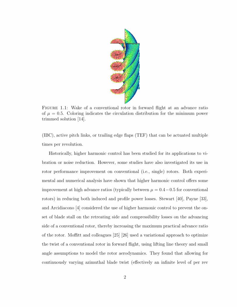
Figure 1.1: Wake of a conventional rotor in forward flight at an advance ratioof µ = 0.5. Coloring indicates the circulation distribution for the minimum powertrimmed solution [14].
(IBC), active pitch links, or trailing edge flaps (TEF) that can be actuated multiple
times per revolution.
Historically, higher harmonic control has been studied for its applications to vi-
bration or noise reduction. However, some studies have also investigated its use in
rotor performance improvement on conventional (i.e., single) rotors. Both experi-
mental and numerical analysis have shown that higher harmonic control offers some
improvement at high advance ratios (typically between µ = 0.4−0.5 for conventional
rotors) in reducing both induced and profile power losses. Stewart [40], Payne [33],
and Arcidiacono [4] considered the use of higher harmonic control to prevent the on-
set of blade stall on the retreating side and compressibility losses on the advancing
side of a conventional rotor, thereby increasing the maximum practical advance ratio
of the rotor. Moffitt and colleagues [25] [26] used a variational approach to optimize
the twist of a conventional rotor in forward flight, using lifting line theory and small
angle assumptions to model the rotor aerodynamics. They found that allowing for
continuously varying azimuthal blade twist (effectively an infinite level of per rev
2

harmonic control) could result in significant reductions in both induced and profile
power, reducing total power by up to 15% at an advance ratio of approximately
µ = 0.35. Hall et al. [17] used a variational approach to determine the minimum
induced loss lift distribution, and determined that at an advance ratio of µ = 0.25,
typical rotors may have 10-15% more induced losses than the minimum induced loss
solution, suggesting that there is room for performance improvement through higher
harmonic control and improved rotor design. Cheng et al. [10] evaluated the use of
2/rev harmonic control to improve the performance of a four-bladed articulated rotor
through decreases in profile losses. The authors found that a properly phased 2/rev
input can decrease required power by about 16% at an advance ratio of µ = 0.32,
primarily through perturbing the angle of attack to change the distribution of the
profile drag coefficient over the rotor disk. In a similar approach to the Reference [17]
work, Rand et al. [36] used an iterative approach to find the optimal circulation dis-
tribution of a single rotor using a free-wake geometry, and found that reductions of
no more than 10% of the induced power can be achieved under any passive or active
blade rotor design for advance ratios less than µ = 0.25.
Beginning in 2004, Ormiston [27, 28] developed a simplified rotor model to explore
the fundamental behavior of rotor induced power at moderate to high advance ratios.
Ormiston also studied the effect of higher harmonic control on rotor performance, and
concluded that higher harmonic control offers promise for reducing induced power,
especially at high advance ratios. Ormiston also found that using the correct level
of blade twist reduces induced power, although the optimal twist distribution varies
with advance ratio. Wachspress et al. [41] used a free-vortex wake model to analyze a
conventional rotor with constant chord, linearly twisted blades and higher harmonic
control. Both 2/rev and 3/rev control inputs with varying phases were analyzed to
determine the phase shifts that would yield power decreases. Among the authors’
findings were that a 3/rev pitch input can reduce induced power by 4% at an advance
3

ratio of µ = 0.2. The authors also suggest that a more formal optimization routine
that includes harmonic cyclic inputs and radial basis functions as design variables
could offer improved insight compared to performing parametric studies that vary
one variable at a time.
Experimental results have also demonstrated the promise of higher harmonic
control in performance improvement. Shaw et al. [38] conducted wind-tunnel tests
that demonstrated up to 6% reduction in power required on a Boeing CH-47D rotor
at 135 kt using 2/rev swashplate control. Jacklin et al. [19, 20] performed wind
tunnel tests on a full-scale BO-105 helicopter rotor using individual blade control,
and found that a 2/rev input could achieve up to a 7% power reduction at high
advance ratios (µ = 0.4− 0.45). However, the 2/rev input resulted in an increase in
power at lower advance ratios.
Another active area of research aimed at improving high speed efficiency in heli-
copters is in the design of coaxial and compound helicopters. Coaxial and compound
helicopters have long demonstrated promise in reducing power requirements in for-
ward flight relative to a conventional rotor. A compound helicopter combines the
hover capabilities of a helicopter with high speed flight capability through the use of a
separate source of propulsive force in addition to the rotor. Frequently, a compound
helicopter also uses a wing to provide additional lift at high flight speeds. Examples
of compound helicopters include the Cheyenne helicopter (Figure 1.2), and, more re-
cently, the Eurocopter X3 (Figure 1.3), which exceeded speeds of 255 knots in level,
stabilized flight [32] and currently holds the world record for the fastest compound
helicopter. A coaxial rotor is defined as a pair of counter-rotating rotors that spin
about a common shaft axis. In the 1970s, the Sikorsky X-59 made use of a coaxial,
rigid rotor in a system referred to as the Advancing Blade Concept (ABC). The
ABC offloads the retreating blade at high speeds, achieving roll trim by balancing
the moments transmitted to the hub by the opposing advancing side blades. This
4
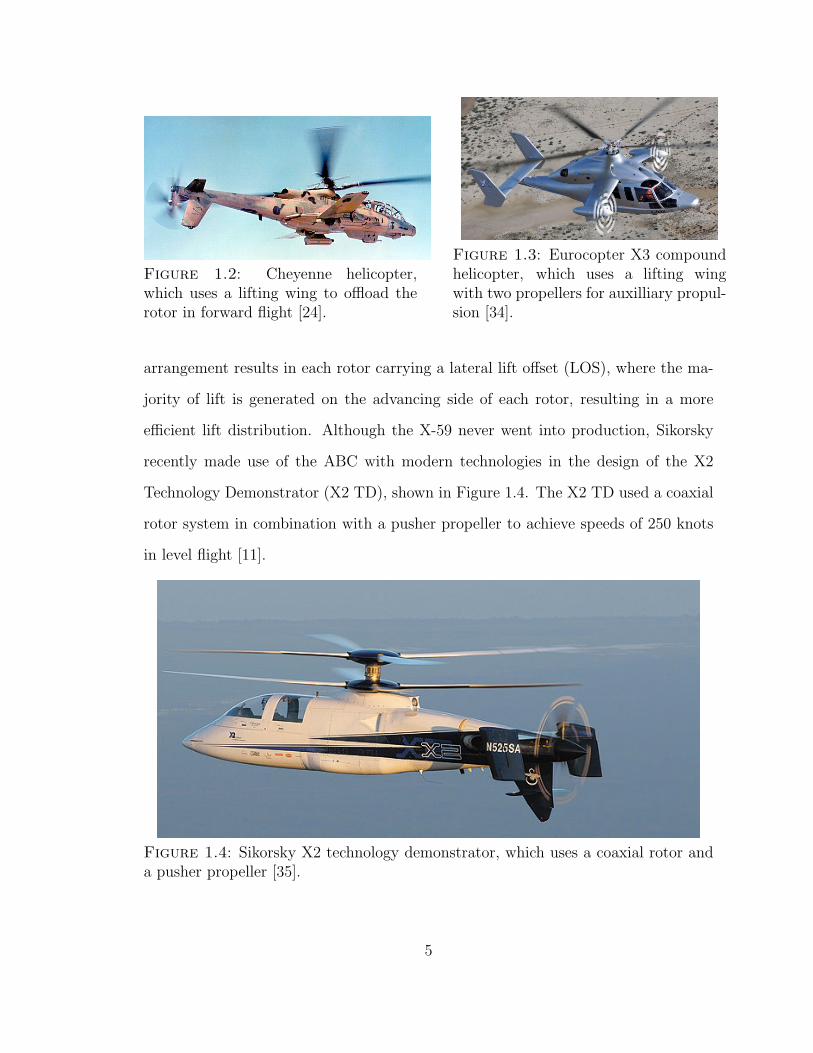
Figure 1.2: Cheyenne helicopter,which uses a lifting wing to offload therotor in forward flight [24].
Figure 1.3: Eurocopter X3 compoundhelicopter, which uses a lifting wingwith two propellers for auxilliary propul-sion [34].
arrangement results in each rotor carrying a lateral lift offset (LOS), where the ma-
jority of lift is generated on the advancing side of each rotor, resulting in a more
efficient lift distribution. Although the X-59 never went into production, Sikorsky
recently made use of the ABC with modern technologies in the design of the X2
Technology Demonstrator (X2 TD), shown in Figure 1.4. The X2 TD used a coaxial
rotor system in combination with a pusher propeller to achieve speeds of 250 knots
in level flight [11].
Figure 1.4: Sikorsky X2 technology demonstrator, which uses a coaxial rotor anda pusher propeller [35].
5

In Reference [5], Bagai describes the aerodynamic design of the X2 TD main rotor
blades, which was driven by high speed flight requirements. The blades make use of
modern airfoils, a non-uniform planform, and a nonlinear twist distribution to reduce
profile losses of the rotor. Induced power losses were not considered in the analysis,
although the author notes that “It is to be expected that induced losses make up
a significant part of the power consumed by the rotor, and careful consideration of
these losses need yet to be made.” Also of interest, the author notes that 2/rev
harmonic control may prove beneficial in improving the aerodynamic efficiency of
the rotor. However, with the exception of the Reference [16] paper that serves as
the foundation for this work, to date no studies have been conducted to evaluate
the use of higher harmonic control in compound and coaxial configurations for rotor
performance improvement.
In addition to the Reference [5] paper, a fair amount of recent research seeks
to understand and improve the performance of compound and coaxial rotors. John-
son [21] used the comprehensive analysis code CAMRAD II to explore the calculated
performance capability of coaxial rotors using lift offset (LOS) rigid rotors. Johnson
performed parametric studies to determine the blade twist, chord, and sweep that
yield the optimal balance of hover and cruise performance. The coaxial configuration
analyzed also includes a small lifting wing and two propellers for additional thrust in
forward flight. Johnson found that a lift offset of about 0.25 is effective in reducing
the rotor induced power and profile power, yielding a rotor effective lift-to-drag ratio
of about 10 at high speeds. Additionally, by comparing free wake and prescribed
wake results, Johnson concluded that a free wake geometry is not required in the
aerodynamic modeling of high advance ratios. References [22] and [37] continue this
work, using CAMRAD II to determine the optimal configuration and sizing for spe-
cific mission requirements. Ormiston [31] used formal optimization techniques with a
compact analytical model for induced power to determine the optimal rotor collective
6

pitch, angle of attack, and linear blade twist for several compound configurations,
and concluded that a full compound using both a wing and auxilliary propulsion
provides the best aerodynamic efficiency. Also of interest, Ormiston concluded that
induced power significantly reduces the aerodynamic efficiency of compound rotor-
craft, and is an important factor in distinguishing between high and low performance
configurations.
Hall and Hall [14], building upon their Reference [17] work on the minimum in-
duced loss lift distribution of helicopter rotors in forward flight, used a variational
approach to compute the theoretical optimal aerodynamic performance of conven-
tional and compound helicopters in trimmed flight. They found that compound and
coaxial configurations can substantially reduce power loss by producing a more ef-
ficient wake structure and by reducing the induced power associated with roll trim.
The optimal circulation distribution minimizes the sum of the induced and viscous
power required to develop a prescribed lift and/or thrust, subject to constraints that
the helicopter be trimmed in pitch and roll. The resulting analysis – which is the
viscous helicopter analog of Goldstein’s inviscid propeller theory [13] – gives rigorous
upper bounds on the performance of conventional and compound helicopters and may
be used to predict the rotor/wing loadings that produce optimal performance. This
analysis does not consider the specific rotor design required to achieve the optimal
circulation distribution; rather, it assumes a “rubber rotor” that can be articulated
with unlimited degrees of freedom to achieve the optimal circulation distribution.
The Reference [14] results raise some very interesting questions. If one is limited
to a finite number of design variables – for example, blade planform, blade twist,
and collective and cyclic blade pitch control – then what is the optimal performance
(minimum power) that can be achieved? Additionally, what design variables are re-
quired to achieve the optimum, and what performance improvements can be achieved
using higher harmonic blade control in conventional, compound, and coaxial rotors?
7

This thesis presents two methods for determining the optimal rotor design for
conventional and compound helicopter configurations using higher harmonic blade
root control. The optimal rotor design minimizes the sum of the induced and viscous
power losses while achieving a prescribed lift and maintaining roll and pitch trim.
Results are presented for the analysis of a conventional rotor, coaxial rotor, and
wing-rotor compound, shedding light on the minimum power of various rotor designs
and the potential benefits of higher harmonic control and optimized blade design.
The work presented here is an extension of the Reference [16] work by Hall and
Giovanetti, which investigated the use of higher harmonic control in conventional
and coaxial configurations.
Chapter 2 summarizes the optimal circulation problem (i.e., the rubber rotor
analysis), which is cast as a variational statement that minimizes the sum of induced
and viscous power required to develop a prescribed lift and/or thrust. The variational
statement is discretized and solved using a vortex-lattice technique.
Chapter 3 describes two approaches to solving the optimal rotor design problem.
The first method, referred to as the Quadratic Programming or QP approach, models
the sectional blade aerodynamics using a linear lift curve, a quadratic drag polar,
and assumes small induced angles of attack. Furthermore, the chord distribution is
fixed, and is not included in the set of design variables. The result is a quadratic
programming problem that yields a set of linear equations to solve for the unknown
optimal design variables. The QP method provides an extremely efficient approach to
calculating optimal rotor performance and design. The second method, referred to as
the Nonlinear Programming or NLP approach, solves the fully nonlinear variational
problem, which accounts for nonlinear lift curves, non-quadratic drag polars, large
induced angles of attack, and includes blade chord as a design variable. An approach
to solving the nonlinear problem via Newton iteration is described. Additionally, a
second approach to solving the nonlinear problem using Mathematical Programming
8

via Augmented Lagrangians is described in Appendix A. The NLP method provides
a more accurate approach to calculating optimal rotor performance and design, and
has the added capability of optimizing the chord distribution. Chapter 3 also includes
a comparison of results to Allen’s computational fluid dynamics analysis [1] of the
Caradonna-Tung rotor [9], demonstrating that the simplified analysis developed here
agrees well with high fidelity CFD calculations.
Chapter 4 describes the optimal rotor design and performance of a conventional
rotor. Results show that 2/rev and 3/rev harmonic control provide large power
reductions at very high advance ratios (µ > 0.5), while offering more modest power
reductions at advance ratios below this. Additionally, results show that the use of an
optimized blade twist and chord distribution provides large power reductions at all
advance ratios; for example, at µ = 0.4, use of an optimized twist distribution and
planform yield a 37% reduction in total power compared to a uniform chord, zero
twist blade. Also of interest, the optimal planform at µ = 0.4, which is representative
of high speed flight in modern helicopters, includes a highly non-uniform planform
with higher solidity than the baseline rectangular blade. This blade design serves to
dramatically reduce induced power and increase efficiency.
Chapter 5 describes results for a coaxial rotor design intended to approximate
the X2 Technology Demonstrator parameters. At the design intent advance ratio of
µ = 0.85, use of 3/rev harmonic control provides a 16% reduction in total power over
conventional 1/rev control. Also of interest, the optimal lift offset at this high speed
is close to 0.5. When making use of a more restrictive lift offset, higher harmonic
control provides significantly larger relative benefits. For example, 2/rev harmonic
control yields a 47% reduction in power versus 1/rev at the design advance ratio with
lift offset constrained to 0.3, the maximum value used on the X2 TD rotor. Analysis of
a single point design shows that higher harmonic control is also effective in improving
the performance of a given blade at off-design points, an encouraging result given the
9

practical limitation to use a fixed blade geometry across all flight conditions. Finally,
results show that induced power losses play a large role in optimum rotor design and
performance.
Chapter 6 gives results for a wing-rotor compound configuration approximating
the Cheyenne helicopter. These results show that use of an optimal wing and rotor
twist distribution and planform yields a 40% reduction in total power at µ = 0.8
compared to an untwisted blade and wing with uniform chord distributions. Higher
harmonic control offers more modest benefits when used in conjunction with the
optimized planforms; however if the optimal high speed wing and rotor design are
not used (perhaps due to hover or low speed requirements), higher harmonic control
is effective at reducing power. Also of interest, use of an off-centered wing results
in decreased power requirements relative to a centered wing of the same span. For
example, for a wing with span equal to one rotor radius, placing the wing entirely on
the retreating side of the rotor results in a 20% reduction in total power compared
to a centered wing. This result suggests that an asymmetric wing could be used in
forward flight to significantly improve vehicle performance.
Finally, Chapter 7 gives concluding remarks and includes a brief discussion of
future work.
10

2
Aerodynamic Modeling of a Rotor
In this section, we briefly describe the aerodynamic models we use to calculate the
forces and moments acting on helicopter rotors, and the resulting induced and viscous
power losses. Additionally, we present a summarized version of the Reference [14]
far field analysis that determines the optimal circulation for minimum power require-
ments, i.e. the rubber rotor solution. The modeling here assumes high aspect ratio
rotor blades, so lifting line theory may be used to calculate induced washes. We as-
sume light loading and/or high advance ratios, so a prescribed wake is appropriate.
Finally, we assume that for the purpose of computing viscous forces (but not inviscid
forces), the flow is quasi-steady. Thus, the sectional lift and drag can be described
using steady two-dimensional lift and drag curves found from experiment or using a
computational fluid dynamic analysis.
2.1 Forces and Moments
Following Hall and Hall [14], we calculate inviscid forces and moments (and also
induced power) using a far-field approach. The forces and moments acting on the
rotor(s) or rotor/wing system are a result of apparent linear and angular momentum
11

Figure 2.1: Schematic of prescribed wake showing one period of the far wakebounded by the Trefftz volume [14].
(i.e., Kelvin linear and angular impulses) deposited in the wake of the rotor. The
Trefftz volume bounds one period of the flow field in the far wake, bounded between
two infinite parallel planes roughly transverse to the flight direction as shown in
Figure 2.1.
The far field flow is assumed to be inviscid, incompressible, and irrotational,
except for the trailing and shed vorticity in the wake. Note that the assumption of
incompressible flow requires only that the induced velocities in the wake be small
compared to the speed of sound, an assumption consistent with the light loading
model. (The flow will in general be compressible in the near field of the rotor.)
Thus, the three-dimensional flow in the far wake is governed by Laplace’s equation
expressed in the fluid frame of reference,
∇2φ = 0 where w = ∇φ (2.1)
where φ is the velocity potential and w is the induced wash.
The net aerodynamic forces acting on a rotor (or any system of rotors and wings)
is equal and opposite to the rate at which the Kelvin linear impulse of the fluid
12

increases. The Kelvin impulse for one period of the wake can be expressed as an
area integral, i.e.,
ξξξ = −ρ∫∫W
Γn dA (2.2)
where the integral is taken over one side of the wake denoted by W , and n is the
unit normal to the wake. Thus, the time-averaged force on the rotor is equal to
F = − ξξξ
T=ρ
T
∫∫W
Γn dA (2.3)
where T is the temporal period of the wake, usually equal to 2π/ΩB because only
one B-th of a turn of the wake is required to achieve periodicity.
Likewise, the time-averaged moment acting on the system is equal to
M =ρ
T
∫∫W
Γ r× n dA (2.4)
where r is the moment arm extending from the center of gravity of the aircraft to
the element of wake area at the time the wake is generated.
2.2 Induced Power
The induced power losses due to lift and thrust of a conventional helicopter rotor, or
rotor/wing/propeller system for a compound helicopter, arise from the deposition of
kinetic energy into the wake. The kinetic energy contained in the Trefftz volume is
given by
E =
∫∫∫V
1
2ρ |w|2 dV =
ρ
2
∫∫∫V|∇φ|2 dV (2.5)
Application of the second form of Green’s theorem, and making use of the periodicity
of the wake in the far-field, the asymptotic decay rate of the wash in the direction
transverse to the direction of flight, and the fact that the potential satisfies Laplace’s
13

equation, one can show that the energy per period of the wake can be expressed as
E = −ρ2
∫∫W
Γw · n dA (2.6)
Hence, the time-averaged induced power Pi, equal to the rate of kinetic energy pro-
duction, is given by
Pi = − ρ
2T
∫∫W
Γw · n dA (2.7)
Note that the induced wash w is linearly related to the circulation Γ through the
Biot-Savart law. Thus, the induced power is quadratic in the circulation. Further-
more, the forces and moments generated by the rotor system are proportional to Γ,
so the induced power will be quadratic in the forces and moments. Also of note, the
induced power may take the form of induced rotor torque (shaft power) or induced
drag. The current approach makes no distinction between these losses. Interestingly,
the induced drag is sometimes not a drag at all, but rather an induced thrust.
2.3 Profile Power
To determine the profile power losses, we make the simplifying assumption that
the aerodynamic surfaces have large aspect ratios, allowing us to model the sectional
aerodynamic forces using quasi-steady sectional lift and drag coefficients as a function
of local angle of attack.
As an example, Figure 2.2 shows the lift and drag computed for a NACA 0012
airfoil operating at a Reynolds number of 10,000,000 for the full range of angles
of attack from −180 to +180 degrees [39]. Note that for small angles of attack
(−14 < α < +14), the lift curve slope is linear and the drag is relatively small.
For larger angles of attack, however, the airfoil is stalled, and the lift and drag can
be quite large, and they behave in a fundamentally nonlinear fashion.
14

-160 -120 -80 -40 0 40 80 120 160Angle of Attack, (deg)
-1.5
-1.0
-0.5
0.0
0.5
1.0
1.5
2.0
Sect
iona
l Coe
ffici
ents
of L
ift a
nd D
rag
Coefficient of Lift, c_lCoefficient of Drag, c_d
Figure 2.2: Computed sectional coefficients of lift and drag for a NACA 0012 airfoiloperating at Re = 10,000,000 [39].
In general, the time averaged profile power Pv may be expressed as the work per
cycle divided by the period, so that
Pv =1
T
∫∫W
1
2ρu2ccd dA (2.8)
where u is the relative velocity of a given airfoil section normal to the span of the
rotor.
We use one of two different drag models. For fully nonlinear calculations, we
spline fit the complete lift and drag curves as a function of angle of attack and
make use of Equation (2.8). However, in the quadratic programming approach to be
discussed in the following section, we make the assumption of small angles of attack.
For these pre-stall small angle of attack cases, it is useful to represent the drag in the
form of a drag polar, cd = cd(c`). Figure 2.3 shows the computed drag polar for the
NACA 0012 airfoil for small angles of attack. Also shown is a quadratic curve fit.
We see that in this unstalled region, the coefficient of drag is very nearly quadratic
in the coefficient of lift, so we may write
cd ≈ cd0 + cd2 (c` − c`0)2 (2.9)
15

-2.0 -1.5 -1.0 -0.5 0.0 0.5 1.0 1.5 2.0Sectional Coefficient of Lift, c_l
0.000
0.005
0.010
0.015
0.020
0.025
Sect
iona
l Coe
ffici
ent o
f Dra
g, c
_d
Curve FitEppler PROFILE code
Figure 2.3: Computed sectional drag polar for a NACA 0012 airfoil operating atRe = 10,000,000 [39]. Also shown is quadratic curve fit to data in unstalled region.
for c`min ≤ c` ≤ c`max. The curve fit shown uses the values cd0 = 0.00651, cd2 =
0.00268, c`0 = 0.0, c`min = −1.421, and c`max = +1.421.
For the case of the quadratic drag polar, Equation (2.8) may be written as a
quadratic function of the circulation. The coefficient of lift may be expressed in
terms of the circulation as
c` =`
12ρu2c
=2Γ
uc(2.10)
Making use of the quadratic drag polar approximation, the viscous power is given by
Pv =ρ
2T
∫∫W
(4cd2
c
)(Γ− Γ0)2 +
(u2ccd0
)dA (2.11)
where Γ0 is the circulation corresponding to a coefficient of lift equal to c`0. Note
that in this form, the viscous power is quadratic in the circulation.
2.4 Optimal Rotor Performance
We first seek to find the unsteady circulation distribution that produces an optimal
solution without regard to the control inputs required to achieve this circulation
distribution. For a more detailed documentation of this approach, see References
[14, 17, 42].
16

We define the optimum circulation distribution to be that which minimizes the
sum of the induced and profile powers subject to lift and trim constraints. Making
use of the calculus of variations, we adjoin the lift and moment trim constraints to
the total power using Lagrange multipliers λλλM and λλλF , respectively. The result is
the Lagrangian power Π, that is,
Π = Pi + Pv + λλλF · (F− FR) + λλλM · (M−MR) (2.12)
where FR and MR are the prescribed time-averaged aerodynamic force and moment
vectors, respectively. Taking the variation of Equation (2.12) and setting the result
to zero, and with the help of some vector identities, yields the generalized Betz
criterion for the case of the fully nonlinear lift/drag curves, that is
w · n = (λλλF + λλλM × r) · n + ucdαc`α
(2.13)
Alternatively, for the case where viscous effects are modeled using the quadratic
drag polar, we require that the circulation not be so large as to result in airfoil
stall. Thus, we adjoin to Π this additional inequality constraint using the Lagrange
multiplier κ, with the result
Π = Pi + Pv + λλλF · (F− FR) + λλλM · (M−MR)
+ρ
T
∫∫Wκ (Γ− Γmax) dA (2.14)
Note κ is nonzero only on regions of the wake where the circulation is large enough
that the stall constraint is in effect. Again, taking the variation and setting the result
to zero gives
w · n = (λλλF + λλλM × r) · n +4cd2
c(Γ− Γ0) + κ (2.15)
Equations (2.13) and (2.15) give the resultant normal wash on the far wake for
an optimally loaded rotor for the fully nonlinear and quadratic drag polars, respec-
tively. Each of these two equations may be thought of as a generalized Betz criterion
17

for optimality [14, 7]. For the fully nonlinear drag curve case, the term u cdα/c`α is
small, except when the lift curve slope goes to zero, that is, as the blade approaches
stall. For the quadratic drag polar case, the term involving cd2 has little effect on the
optimum circulation, and in fact cd0 does not appear at all. If the stall inequality con-
straint is not active at some radial and azimuthal location, then κ = 0 everywhere,
and the last term has no effect. The effect of the terms u cdα/c`α in Equation (2.13)
and κ in Equation (2.15) is to reduce the optimal downwash in regions approaching
stall. Furthermore, for both cases, while profile power certainly contributes signifi-
cantly to the total power, if the rotor is not constrained by stall, then the optimum
circulation distribution is (very nearly) found by minimizing induced losses – at least
for a prescribed planform.
2.5 Vortex Lattice Model
In the previous sections, we outlined an analytical description of the minimum power
solution for a rotor in forward flight. As a practical matter, to solve for the optimum,
we must discretize the relevant equations. To calculate the optimal aerodynamic
power and corresponding circulation distribution, we represent the wake trace using
a lattice of vortex rings, which can model both trailing and shed vorticity in the wake.
One period of the wake trace (the reference period) is divided into M quadrilateral
elements (see Figure 2.4). The ith element is a quadrilateral vortex ring with filament
strength Γi. Thus, the potential jump across the ith element is just Γi, and the time-
averaged force and moment on the helicopter may be approximated by
F =ρ
T
M∑i=1
ni ∆AiΓi =M∑i=1
biΓi = B ΓΓΓ (2.16)
M =ρ
T
M∑i=1
ri × ni ∆AiΓi =M∑i=1
diΓi = D ΓΓΓ (2.17)
18

Figure 2.4: Wake due to one complete rotation of a four-bladed rotor in forwardflight with advance ratio µ = 0.5 as viewed from above. The wake is represented byquadrilateral vortex rings. Note that because of the periodicity in the problem, afour-bladed rotor can be modeled by just one quarter turn of the wake; a full turn isshown here for clarity.
Likewise, the total power loss is approximated by
P =1
2
M∑i=1
M∑j=1
KijΓiΓj −M∑i=1
QiΓi + Pv0
=1
2ΓΓΓTK ΓΓΓ−ΓΓΓT Q + Pv0 (2.18)
with
Kij = − ρT
wij · ni ∆Ai + δijρ
T
[4cd2
c
]i
∆Ai (2.19)
Qi = 2ρ
Tui [c`0cd2]i ∆Ai (2.20)
Pv0 =ρ
2T
M∑i=1
u2i
[c(cd0 + cd2c`
20
)]i∆Ai (2.21)
19

making the discretized form of the Lagrangian power
Π =1
2ΓΓΓTKΓΓΓ−ΓΓΓTQ + Pv0 + λλλF · (BΓΓΓ− FR) + λλλM · (DΓΓΓ−MR) (2.22)
Minimizing the power, which is quadratic in the circulation, subject to lift and
trim constraints that are linear in circulation is a so-called quadratic programming
problem. Using the calculus of variations, we find the solution is given by
12(K + KT ) BT DT
B 0 0D 0 0
ΓΓΓλλλFλλλM
=
QFR
MR
(2.23)
Note Eq. (2.23) is linear, making it particularly easy to solve. However, the computed
optimum circulation must be checked to determine whether any portion of the rotor
blade has a circulation resulting in a coefficient of lift exceeding the stall limits. If so,
one must introduce the stall inequality constraints making the problem nonlinear.
Equation (2.23) describes the minimum power solution for a rubber rotor, allow-
ing one to solve directly for the optimal circulation distribution without regard to
the blade control or planform required to achieve this distribution. For real aircraft,
however, one will not be able to obtain the optimum rubber rotor circulation dis-
tribution because the number of inputs to the system is finite. In the next chapter,
we consider the optimum performance of real rotors with a finite number of design
variables and control inputs including fixed radial blade twist and chord distributions
and conventional and higher harmonic blade control.
20

3
Optimal Rotor Control and Design
The previous chapter outlines a method to solve for the optimal circulation distri-
bution of a helicopter rotor with no regard to the control inputs required to achieve
this circulation distribution. This is referred to as the rubber rotor solution, and
represents the optimal performance achievable if the rotor could be articulated with
infinite degrees of freedom, providing a rigorous upper bound on the performance of
a rotor.
In this chapter, two techniques are presented to solve for the optimal circulation
distribution subject to the constraint that the circulation is realizable using a given
set of design variables and control inputs. The first method, outlined in Section 3.2 is
a quadratic programming (QP) approach. The QP formulation assumes small angles
of attack, a linearized lift curve (i.e. no stall at high angles of attack), and a quadratic
drag polar (as shown in Figure 2.3). Additionally, the QP approach is not capable
of optimizing the blade chord as a design variable, although any arbitrary fixed
chord distribution can be analyzed with this method. The second method, outlined
in Section 3.4, is a Nonlinear Programming (NLP) approach. The full nonlinear
formulation of the problem is solved with Newton iteration. Additionally, a second
21

approach to solving the nonlinear problem is described in Appendix A. This technique
uses Mathematical Programming via Augmented Lagrangians using the Broyden-
Fletcher-Goldfarb-Shanno (BFGS) gradient based variable metric method [8] to solve
the successive unconstrained minimization problems.
3.1 Defining Design Variables
In the design of a rotor, one may select a fixed blade twist distribution θ0(r), and
also implement some limited set of harmonic blade pitch control inputs. For such
a configuration, the blade twist as a function of radius r and azimuth ψ can be
described as
θ(r, ψ) = θ0(r) + A0 +N∑n=1
An cos(nψ) +N∑n=1
Bn sin(nψ) (3.1)
where An and Bn are the Fourier coefficients of the blade pitch and N is the number
of harmonics in the higher harmonic control system. A conventional helicopter with
collective and cyclic control corresponds to N = 1.
We denote the total vector of design variables by Θ. This vector is comprised of
two distinct vectors
Θ =
Θθ
Θc
(3.2)
where Θθ contains the design variables that affect the pitch angle of the blade or
wing, including the fixed radial twist and some form of azimuthal pitch control, such
as a root pitch input or some other method such as the use of spanwise flaps. Θc then
contains the design variables that affect the chord distribution. For a harmonic blade
pitch control scheme as shown in Equation (3.1), the vector Θθ will be comprised
of the Fourier coefficients of blade pitch A0, An, and Bn, and θ0(r) at a discrete set
of radii. Alternatively θ0(r) may be represented by a summation of shape functions
22

in the radial direction, in which case the coefficients of the shape functions would
be members of Θθ. Similarly, if the chord distribution is to be optimized, Θc will
contain either the value of the chord at a discrete set of radii or the coefficients of
the shape functions that describe the chord distribution. We define the number of
elements in Θθ as f and the number of elements in Θc as g. We define the total
number of design variables as h, which is of course equal to f + g.
The vector Θ relates some limited set of design variables to the blade pitch and
chord at every panel in the vortex lattice grid. We denote the pitch angle at each
panel due to the design variables as the vector θ and the chord at each panel as the
vector c. These vectors both have length M , where M is the number of panels in
the vortex lattice grid. It will be useful in the following derivations to define a set of
matrices that transform Θ or some portion of Θ into the values of twist and chord
at each panel as follows: θc
= StotalΘ (3.3)
θ = SθΘθ (3.4)
c = ScΘc (3.5)
Lastly, when implementing certain chord constraints it is advantageous to expand
Θc into a vector representing the chord at a single set of panels along the span of a
blade, cspan. We define ScRadial such that
cspan = ScRadialΘc (3.6)
The entries of each of the S matrices will depend on the global or local shape functions
used to represent blade twist and chord.
23

3.2 Quadratic Programming Approach
3.2.1 Motivation
To compute the forces, moments, and power on a rotor, we must find the circulation
in terms of the design variables contained in Θ. In this study, we use a lifting-line
approximation to compute the wash on the blades. Using our lightly loaded model,
the induced wash is a linear function of the circulation. However, the resulting
induced angles of attack on the rotor blade can be large, especially in and near
the reverse flow region – large enough to require the use of a nonlinear lift curve –
rendering the circulation a nonlinear function of the control inputs. The circulation
is also a nonlinear function of the blade chord, so for problems involving chord
optimization, these nonlinearities cause the power to be non-quadratic in the design
variables, and the constraints to be nonlinear. An approach to solving this nonlinear
optimization problem is discussed in Section 3.3.
In general, nonlinear constrained optimization problems are difficult and expen-
sive to solve. In this section, we propose a very efficient small disturbance formulation
of the optimization problem. To make the nonlinear optimization more tractable, we
first approximate the angles of attack as small, the lift curve as linear, and the drag
curve as quadratic. Additionally, we do not include chord variables in the vector
of design variables to be optimized, meaning we only consider the vector of pitch
angle inputs Θθ as optimization variables. Based on these assumptions, the power is
quadratic in circulation and the problem can be solved using quadratic programming,
similar to the approach to solving the rubber rotor optimization problem described
in Section 2.5.
24

3.2.2 Method
To efficiently solve for the optimal controls, we use the Prandtl lifting-line approxi-
mation with a near-field vortex lattice model of the wake to relate the control inputs
Θ to the near field circulation ΓNF and the wash on the blade w. The induced wash
at the blade is calculated using the the rigid wake model of quadrilaterals described
in Section 2.5 and shown in Figure 2.4, with the exception that each radial line of
panels only accounts for the influence of those panels that preceded them in time,
i.e., the wake is semi-infinite, extending backwards in the direction opposite of flight.
Through the use of the Biot-Savart law, we form the influence coefficient matrix M
that relates the circulation in the wake to the normal component of induced wash at
the blade. The linearized lifting line equation at the ith station in the wake, assuming
incompressible flow, can be written as
2ΓNFi
uici(c`α)i+ αindi = αgeoi (3.7)
where c`α is the lift curve slope, c is the chord, αind is the induced angle of attack,
and u is the relative fluid velocity perpindicular to the span of the blade.
To account for compressibility effects, the Prandtl-Glauert transformation is used
to modify c`α based on the local Mach number, Mi, resulting in the compressible
version of Equation (3.7), that is,
2Γi√
1−Mi2
uici(c`α)i+ αindi = αgeoi (3.8)
The induced angle of attack αind is a function of the normal component of induced
wash at the blade wi and the local velocity ui. We make use of the small angle
approximation: tan(α) ≈ α, so that αindi ≈ wi
ui. Thus, in this approximation, the
induced angle of attack is linear in the circulation. The induced angle of attack at
25

each panel in the discretized wake can then be related to the circulation ΓNF through
the matrix Wα
αind = WαΓNF (3.9)
with the entries of Wα given by
Wαij =Wij
ui(3.10)
Combining Equation (3.7) and the Equation (3.9) expression for αind gives
ALLΓNF = αgeo (3.11)
with the entries of ALL for the compressible case given by
ALLij =2δij√
1−Mi2
uici(c`α)i+Wαij (3.12)
where δij is the Kronecker delta function. The circulation can be found from Equa-
tion (3.9) by inverting the matrix ALL, yielding
ΓNF = ALL−1αgeo (3.13)
The unknown quantity we wish to solve for is the vector of design variables,
Θθ. It is therefore advantageous to separate the angle αgeo into two components:
an angle of attack resulting from the initial position of the blade with zero control
inputs, called α0, and an angle resulting from the control inputs pitching the blade
by some amount, called θ. αgeo is then equal to the sum of these two angles, making
Equation (3.13)
ΓNF = ALL−1α0 + ALL
−1θ (3.14)
We now use the Sθ matrix to expand Θθ, the vector of design variables, into the
vector θ, which contains the pitch angle change due to the design variables at each
panel in the grid. Substituting SθΘθ for θ gives
ΓNF = ALL−1α0 + ALL
−1SθΘθ (3.15)
26

Next, we relate the near field circulation to the far field circulation, and use the
methods of Section 2 to calculate induced and viscous power, moments, and forces
from the far field circulation. For the Prandtl lifting line approximation, this involves
a trivial mapping of the bound circulation on the rotor blade to its corresponding
position in the far wake, such that
ΓFF = ΓNF (3.16)
For simplicity, we will denote Γ0 = ALL−1α0 and A = ALL
−1Sθ, giving the
following simplified equation for the far field circulation:
ΓFF = AΘθ + Γ0 (3.17)
The vector Γ0 is the circulation due to zero control inputs (an untwisted blade rotat-
ing with no pitch relative to the axis of rotation), and can therefore be determined
by the geometry of the wake, which in turn is entirely determined by known variables
such as the rotor disk angle of attack and the advance ratio of the vehicle. The only
unknown is the small vector of design variables Θθ. Substituting Equation (3.17)
into Equation (2.22) gives the Lagrangian power in terms of the control inputs. Set-
ting the variation of this equation to zero for small variations in the design variables
and Lagrange multipliers gives the desired system of linear equations, that is,
12AT(K + KT)A ATBT ATDT
BA 0 0DA 0 0
Θθ
λF
λM
=
AT(Q−KΓ0)
FR −BΓ0
MR −DΓ0
(3.18)
Equation (3.18) is solved for the unknown design variables that minimize power
for trimmed flight subject to the lift and moment constraints. Once the optimal
design variables are known, the resulting circulation distribution is calculated using
Equation (3.17). The minimum induced and viscous power losses are then calculated
from the far field circulation distribution using Equations (2.16), (2.17), and (2.18).
27

The QP method, as we shall see, gives reasonably accurate results compared to
a full nonlinear search algorithm, but at a fraction of the computational cost. For a
single flight condition, the method requires just a few minutes of computational time
using a single processor computer, and is thus useful for applications requiring the
analysis of many flight conditions. Note that Equation (3.18) assumes small angles
of attack, a linear lift curve slope, and a quadratic drag polar, and therefore does
not account for the effects of stall at high angles of attack. In the QP formulation
we can only solve for the vector Θθ that contains design variables that affect blade
pitch angle (radial blade twist and root pitch inputs, for example). This method is
not capable of solving for optimal chord design variables, although a non-uniform
chord distribution can be analyzed with the QP approach by including a prescribed
chord distribution in Equation (3.12).
Accounting for large angles of attack, nonlinear lift curves, non-quadratic drag
polars, and including the chord distribution as a design variable to be optimized
renders the problem nonlinear, and introduces additional inequality constraints. Two
approaches to solving this nonlinear problem are outlined in the following section.
3.3 Nonlinear Optimization Overview
3.3.1 Motivation
The quadratic programming approach described in the preceding sections assumes
a linear lift curve, meaning that stall at high angles of attack is not modeled. Of
course, a real airfoil will exhibit stall at certain high angles of attack, as shown in
Figure 2.2. Additionally, the previous analysis assumes a quadratic drag polar, which
is only a valid assumption in the unstalled region. Inboard portions of a helicopter
blade in forward flight experience high angles of attack on the retreating side of the
rotor as they enter and exit the reverse flow region, and modeling these high angle
of attack aerodynamics may be important for accurate power predictions.
28

In the optimal circulation model described in Section 2.4 and Reference [14], a
constraint on the maximum and minimum coefficient of lift is implemented with
Mathematical Programming via Augmented Lagrangians to account for realistic co-
efficients of lift and drag. However, when optimizing rotor geometric design variables
rather than circulation, constraining the maximum and minimum coefficients of lift
is not an effective approach. With limited design variables, it may be necessary
to accept some blade stall to achieve the overall optimum solution. As a result,
it is better to accurately model the high angle of attack aerodynamics rather than
constrain the rotor design to avoid this region altogether. Finally, solving the full
nonlinear optimization problem allows for the inclusion of chord design variables into
the optimization, allowing the planform to be formally optimized.
3.3.2 Nonlinear Iterative Lifting Line Method
We first present a method to calculate the circulation from a given set of rotor design
variables in a way that accounts for a nonlinear lift curve and a non-quadratic drag
polar, i.e. one that is effective for arbitrary airfoils. We use the numerical nonlinear
iterative lifting line method described in References [2] and [3]. This approach uses
the vortex-lattice model of the wake described in Sections 2.5 and 3.2 to iteratively
compute the circulation resulting from a given set of design variables. The method
uses tabular airfoil data to account for the effects of high angles of attack on sectional
lift and drag coefficients. The algorithm is:
1. Assume an elliptical circulation distribution along the span of the blade at all
azimuthal points in the wake.
2. Calculate the induced angle of attack at each panel using this assumed circu-
lation distribution. With a prescribed circulation, the normal component of
29

induced wash is given by
w = WΓ (3.19)
with W based on the near field vortex lattice model described in Sections 3.2
and 2.5. The induced angle of attack at the ith panel, αindi, can be calculated
directly as αindi = tan−1(wi
ui), as there is no need to linearize this term with the
small angle approximation. This can make a significant difference in regions of
the wake with large induced angles of attack, such as on the retreating side of
the rotor where the velocity perpindicular to the span of the panel u is small
relative to the induced wash w, making the small angle assumption a poor
approximation of the induced angle of attack.
3. Calculate the effective angle of attack at each panel αeffi using the induced
angle of attack calculated in step 2, the angle of attack of the blade due to the
geometry of the wake, α0i, and the angle of attack at each station resulting
from the design variables, θi. In total, the effective angle of attack is given by
αeffi = α0i + θi − αindi (3.20)
4. Use tabular experimental or numerical data for a given airfoil to determine the
appropriate sectional coefficient of lift, cli, at each panel based on the effective
angle of attack. This is implemented with a lookup table of the Reference [39]
airfoil data interpolated using cubic splines. To account for compressibility,
the value of cli is modified by the Prandtl-Glauert transform,
clcompressible =clincompressible√
1−M2(3.21)
C-81 airfoil data tables, which give the coefficient of lift as a function of effec-
tive angle of attack and Mach number, can also be used as the look-up table,
30

eliminating the need to perform the Prantl-Glauert transform and providing
more accurate estimates of compressible effects.
5. Calculate the circulation at each panel based on the value of the sectional lift
coefficient using
Γi =1
2uicicli (3.22)
6. Update the previous guess of the circulation distribution, Γn−1, using the values
Γ obtained in step 5 with the following formula
Γn = Γn−1 +D(Γ− Γn−1) (3.23)
where D is a damping factor used to prevent the iteration from becoming
unstable. In general, this iteration must be heavily damped, with values of D
ranging from 0.05 - 0.1.
7. Compare the Γn and Γn−1 distributions to determine if convergence has been
reached. If the iteration has not converged, return to step 2, using Γn+1 as the
initial guess at circulation.
The iteration typically reaches convergence within 100-1000 iterations, depending
on the damping used, the number of panels in the grid, the initial guess at circu-
lation, and the controls being evaluated. When performing an optimization that
incrementally updates the control vector, such as the Newton iteration described in
Section 3.4, it is advantageous to use the previous vector of design variable’s circula-
tion distribution as the initial guess at circulation in Step 1 to speed up convergence.
Although this iterative method requires a high number of iterations, it requires
only a single matrix-vector multiplication per iteration, while all other operations
involve updating values within a single vector. As a result, even for grids with a large
31

number of panels, this method converges in a very short amount of computational
time, typically under one or two seconds on a single processor machine.
Once the circulation distribution is known, the forces, moments, and induced
power losses are calculated using the far wake approach approach described in Sec-
tions 2.1 and 2.2. Because the effective angle of attack is known at each panel
following the iteration, sectional drag coefficients can be found found using a lookup
table interpolated with cubic splines. The viscous power loss is then calculated using
a discretized version of Equation (2.8).
3.4 Newton Iteration
3.4.1 Motivation
We have outlined a nonlinear approach for finding the circulation distribution, forces,
moments, and power loss due to a given set of design variables. We now wish to
determine the design variables that result in the minimum power loss while satisfying
constraints on lift and moments. We use one of two methods for solving this nonlinear
constrained optimization problem. The first approach, described in Appendix A,
uses the technique of Mathematical Programming via Augmented Lagrangians, with
the unconstrained minimization phase of this technique solved using the Broyden–
Fletcher–Goldfarb–Shanno (BFGS) variable metric method [8]. The gradients of
the augmented cost function are found using adjoint automatic differentiation. The
primary drawback of this approach is that it is computationally very slow. A given
rotor configuration at a single advance ratio can take over 24 hours to converge,
depending on the grid resolution. Additionally, there are many parameters, such as
weighting values on penalty terms and constants used in the step size search, that
must be varied by trial and error to get a solution that converges in a reasonable
amount of time.
In this section, we present a method for solving the constrained nonlinear opti-
32

mization problem using Newton iteration. This approach approximates the circu-
lation as linear about some set of design variables. The change in design variables
required to satisfy all of the constraints and minimize power to first order accuracy
can then be found by solving a system of linear equations, in a manner similar to
the QP method described in Section 3.2. Since the relationship between circulation
and design variables is nonlinear, this process must be done repeatedly, with the
circulation linearized about a new baseline set of design variables at each successive
step.
This method has several advantages over the Mathematical Programming via
Augmented Lagrangians technique presented in Appendix A. First, it is much more
computationally efficient, and typically converges in fewer iterations. Second, we
can avoid the use of penalty functions that require arbitrary weighting functions to
enforce the equality constraints, since at each iteration the linearized problem will
satisfy the constraints to first-order exactly.
3.4.2 Linearizing the Circulation About a Set of Design Variables
We know that the circulation is a nonlinear function of the design variables
Γ = Γ(Θ) (3.24)
We can also define the residual as
R = R(Γ,Θ) = 0 (3.25)
where R is a system of nonlinear equations describing the relationship between the
circulation and the rotor design variables. In the present analysis, we use the non-
linear lifting line analysis described in Section 3.3.2, but R could also describe some
other numerical method for computing the circulation in terms of the design vari-
ables, e.g., a panel method. We want to approximate the circulation at a new set of
33

design variables as a linear function of the change in controls. If we have a known
circulation Γ0 about an initial set of design variables Θ0, the circulation at design
variables Θ = Θ0 + ∆Θ, can be approximated to first order as
Γ ≈ Γ0 + A∆Θ (3.26)
where the matrix A is defined as
A =∂Γ
∂ΘT(3.27)
The matrix A relates a change in the design variables vector, which can include a
change in the chord distribution, to a linear change in the circulation. Of course,
because the circulation is a nonlinear function of the design variables, Equation (3.26)
is only correct to first order in ∆Θ. We compute the entires of A by Taylor expanding
to first-order the statement of sectional lift given by the Kutta-Joukowski theorem
(L = ρUΓ) in terms of small changes in local angle of attack and chord. This process
is described in further detail in Section 3.4.4.
Because induced power is quadratic in circulation (Pi = 12ΓTKΓ), through Equa-
tion (3.27) we can approximate the change in induced power due to a change in the
design variables.
To optimize the total power, or the sum of the viscous and induced powers, we
must also express the first-order change in viscous power in terms of a change in
design variables. However, viscous power is not directly related to the circulation
distribution. Instead, we define a vector Kv such that
Kv =∂Pv
∂ΘT(3.28)
i.e., Kv relates a change in design variables to the resulting first-order change in
viscous power loss. Thus,
Pv ≈ Pv0 + KTv ∆Θ (3.29)
34

where Pv0 is the viscous power about some initial set of design variables. We deter-
mine the entries of the Kv vector by Taylor expanding to first-order the expression
for viscous power for small changes in chord and angle of attack. This process is
detailed in Section 3.4.5.
3.4.3 Formulating the Variational Problem
To formulate the variational problem, we start with the statement of Lagrangian
power from Section 2.5:
Π =1
2ΓTKΓ + Pv + λF
T (BΓ− FR) + λMT(DΓ−MR) (3.30)
Plugging the expression for circulation found in Equation (3.26) into Equation (3.30)
and including the linearized viscous power loss given in Equation (3.29) gives
Π =1
2(Γ0 + A∆Θ)TK(Γ0 + A∆Θ) + Pv0 + KT
v ∆Θ + λFT (B(Γ0 + A∆Θ)− FR)
+ λMT (D(Γ0 + A∆Θ)−MR)
(3.31)
Taking the variation of Equation (3.31) and setting the result to zero for arbitrary
variations in the change in design variables ∆Θ and Lagrange multipliers gives the
following set of linear equations:
12AT(K + KT)A ATBT ATDT
BA 0 0DA 0 0
∆ΘλF
λM
=
−ATKΓ0 −Kv
FR −BΓ0
MR −DΓ0
(3.32)
To perform an inviscid analysis (i.e., to minimize induced power only), the Kv term
is simply set to zero. At each step of the iteration, this system of equations is solved,
satisfying the equality constraints and minimizing the induced or total power to first
order. The vector of design variables is then updated at each iteration as follows:
Θk+1 = Θk +D∆Θ (3.33)
35

where D is an under-relaxation factor discussed further in Section 3.4.7. Of course, if
D = 1, the linearized circulation at controls Θk+1, which will satisfy all constraints,
is simply
Γk+1 = Γk + A∆Θ (3.34)
However, since this linearized relationship is only a first-order approximation, the
residual R(Γk+1,Θk+1) will be non-zero. It is necessary to calculate the accurate,
nonlinear circulation at Θk+1 after each each iteration using the nonlinear iterative
lifting line procedure described in Section 3.3.2, i.e., to determine the circulation
distribution Γ that makes R(Γ,Θk+1) = 0. As the iteration steps closer to the true
solution and the step sizes become smaller, the linear approximation of circulation
will be more and more accurate, causing the residual to decrease until the solution
converges.
In summary, the algorithm for the Newton iteration is:
1. Select an initial guess at the vector of design variables, Θ, and use this as Θk
on the first iteration.
2. Find Γk based on Θk using the nonlinear iterative lifting line method.
3. Use Γk and Θk to form the matrix A, defined as the first order change in
circulation due to a change in design variables.
4. Assemble and solve the linear system of equations given in (3.32).
5. Update the vector of design variables: Θk+1 = Θk + D∆Θ, where D is an
under-relaxation factor.
6. Set Θk := Θk+1 and return to step 2 until the iteration has converged.
36

3.4.4 Determining the Entries of the A Matrix
To determine the entries of the A matrix, we start with the following expression for
circulation at each panel, obtained from equating the lift calculated by the Kutta-
Joukowski theorem with the definition of the sectional coefficient of lift:
Li = ρuiΓi =1
2ρui
2ci (c`α)i αi (3.35)
Solving for Γi gives,
Γi =1
2uici (c`α)i αi (3.36)
Taylor expanding this equation and retaining first-order terms to approximate ∆Γi
due to changes in the local angle of attack αi and local changes in chord ci gives
∆Γi =1
2uici (c`α)i ∆αi +
1
2uicli∆ci (3.37)
The ∆αi term can be replaced by the sum of two distinct changes in angle of attack:
a change in the induced angle of attack, ∆αindi, and a change in the angle of attack
due to a change in the design variables vector, which will be referred to as ∆θi. Thus,
∆Γi =1
2uici (c`α)i (∆θi −∆αindi) +
1
2uicli∆ci (3.38)
Next, we wish to put ∆αindi in terms of a change in the circulation distribution,
∆Γ. Starting with the following definition
αindi = tan−1
(wiui
)(3.39)
and Taylor expanding Equation (3.39) in terms of the induced wash, wi, and retaining
first order terms gives
∆αindi =
1
1 +(wi
ui
)2
∆wiui
(3.40)
37

The wash at each panel is related to the circulation through the influence coefficient
matrix W :
w = WΓ (3.41)
and therefore, to first order
∆w = W∆Γ (3.42)
and for the ith panel,
∆wi = Wi∆Γ (3.43)
where Wi is the ith row of the matrix W. Substituting Equation (3.43) into Equa-
tion (3.40) and simplifying gives the following expression for ∆αindi, i.e.,
∆αindi =
(ui
ui2 + wi2
)Wi∆Γ (3.44)
Substituting this expression into Equation (3.38) and reorganizing terms gives
∆Γi +1
2ci (c`α)i
(ui
2
ui2 + wi2
)Wi∆Γ =
1
2uici (c`α)i ∆θi +
1
2uicli∆ci (3.45)
Writing this equation in matrix form gives
RΓ∆Γ = RθFull
(∆θ∆c
)(3.46)
with the elements of matrix RΓ defined as follows:
RΓij = δij +1
2ci (c`α)i
(ui
2
ui2 + wi2
)Wij (3.47)
and with RθFull made up of two diagonal matrices, Rθ and Rc, with their elements
defined in Equations 3.49 and 3.50:
RθFull = Rθ|Rc (3.48)
38

Rθij = δij1
2uici (c`α)i (3.49)
Rcij = δij1
2uicli (3.50)
Note that in Equation (3.46) the vector ∆Γ is of length M , where M is equal to
the number of panels in the vortex lattice grid. The vectors ∆θ and ∆c are each of
length M , and the matrix RθFull has dimensions M × 2M .
Finally, to relate a small change in the vector of design variables Θ to the change
in circulation, we use the Stotal matrix to define RΘ as
RΘ = RθFullStotal (3.51)
allowing Equation (3.46) to be written as
∆Γ = RΓ−1RΘ∆Θ (3.52)
The matrices RΓ and RΘ are the Jacobians of R with respect to Γ and Θ,
respectively. Lastly, defining
A = RΓ−1RΘ (3.53)
we have formed a single matrix A of dimensions M×h that relates the change in each
design variable to the corresponding change in circulation to first order accuracy, as
stated in Equation (3.27). Note that this matrix A is very similar to the matrix of
the same name used in the QP approach. There are, however, a couple of important
differences. First, the QP approach does not account for any changes in chord, and
therefore does not include any of the Rc terms given in Equation (3.50). Second,
the QP approach assumes small induced angles of attack, and does not include the
Taylor expansion of the arctangent term, instead simply using the induced angle of
attack as an approximation for the arctangent.
39

3.4.5 Determining the Entries of the Vector Kv
We start with the following equation for the viscous power loss at each discrete panel
in the wake
Pvi =ρu2
i
2cicdi∆Ai (3.54)
where ∆Ai is the area of the ith panel in the wake. Taylor expanding in terms of
changes in the chord distribution, c, and changes in the coefficient of drag due to
changes in the angle of attack θ, and retaining first order terms yields
∆Pvi =ρu2
i
2(∆cicdi + ci (cdα)i ∆αi) ∆Ai (3.55)
Expressing the change in angle of attack as two separate components, one due to a
change in induced angle of attack and one due to a change in design variables, and
using the expression for ∆αindi from Equation (3.44) gives
∆Pvi =ρu2
i
2
(∆cicdi + ci (cdα)i ∆θi − ci (cdα)i
(ui
ui2 + wi2
)Wi∆Γ
)∆Ai (3.56)
Using Equation (3.27) to replace ∆Γ, and including the matrices Sθ and Sc to put
changes in pitch angle ∆θ and chord ∆c at each panel in terms of the change in
design variables ∆Θθ and ∆Θc, gives the following equation
∆Pvi = PTc Sc∆Θc + PT
θ Sθ∆Θθ −PTΘWA∆Θ (3.57)
This equation shows that the first-order change in viscous power has distinct con-
tributions from the change in chord design variables ∆Θc and the change in pitch
angle design variables, ∆Θθ. Additionally, there is a third term that results from
the change in circulation due to the change in the entire design variables vector ∆Θ.
The elements of the vectors Pc, Pθ and PΘ are defined as follows
Pci =ρu2
i
2cdi∆Ai (3.58)
40

Pθi =ρu2
i
2ci (cdα)i ∆Ai (3.59)
PΘi =ρu2
i
2ci (cdα)i
(ui
ui2 + wi2
)∆Ai (3.60)
We want to combine the terms on the right hand side of Equation (3.57) into a single
vector, Kv, such that
∆Pv = KTv ∆Θ (3.61)
To form the Kv matrix, we make use of the fact that the vector ∆Θ is simply a
concatenation of the ∆Θθ and ∆Θc vectors, as shown in Equation (3.2), allowing us
to sum components of Equation (3.57) as follows
Kv =
STθ Pθ
STc Pc
+
ATWTPΘ
(3.62)
Note that the vector ATWTPΘ is of length h, meaning it has an entry for each design
variable. The vector STθ Pθ has an entry for each twist design variable, while the
vector STc Pc has an entry for each chord design variable, making the concatenation
of these two vectors of length h as well and allowing the two vectors to be summed.
3.4.6 Additional Constraints
Two additional constraints are useful for certain configurations: an equality con-
straint on the solidity of the rotor, and a set of local inequality constraints on the
chord distribution.
Solidity Constraint
It is useful in some circumstances to constrain the thrust weighted solidity of the
rotor. As will be discussed in Chapter 5, for coaxial rotors at high forward flight
speeds it is aerodynamically optimal to have a very small chord along the entire
span of the blade, as the high dynamic pressure on the advancing side of the rotor
41

requires very little lifting surface to achieve the required lift. Such a rotor is of little
practical interest, however, since it would be unable to hover or fly at low speeds.
While a chord inequality constraint can be used to prevent excessively small chord
values at each radial station, it gives little flexibility to the optimization routine to
select a planform, as the planform is essentially prescribed by the minimum chord
values. Constraining the thrust weighted solidity ensures adequate blade area while
still allowing the optimization to tailor the planform to the aerodynamic optimum.
The inequality constraint on chord is still used to prevent negative and infinitesimal
chords.
The thrust weighted solidity of the rotor is defined as
σTW ≡3
R3
∫ R
0
σ(r)r2dr (3.63)
This parameter weights the effects of chord at the tip more heavily than at inboard
stations, as changes in the chord further outboard have a larger effect on the thrust
of the rotor due to the higher rotational velocities at these stations. Because the
thrust weighted solidity heavily weights chord at the blade tip, and because the
circulation goes to zero at the tip regardless of the chord, we found that such a
constraint produced oddly shaped tip geometries. To alleviate this problem, we
constrain instead a modified thrust weighted solidity defined by
σTWM ≡3
R3
∫ R
0
r2σ(r) · 1− exp[−(1− r/R)/ε] dr (3.64)
where ε is some constant, typically 0.1. This definition has the effect of reducing
the impact of the chord near the tip on solidity, allowing the tip chord to be its
aerodynamic optimum rather than being artificially inflated to boost solidity.
Regardless of which definition of solidity is used, the equality constraint on so-
42

lidity takes the following form
σconstraint = σ − σreq = 0 (3.65)
where σ is the solidity of the rotor (based on whichever definition of solidity is used)
and σreq is the required solidity. It is possible to implement the solidity constraint
as an inequality constraint in order to place a minimum or maximum value on the
rotor’s solidity. For simplicity, however, we will implement this constraint as an
equality constraint.
Solidity is linearly related to the vector of design variables through Equation (3.63)
or a similar sum if using the tip weighted solidity. This sum is expressed as the dot
product of the vector E and the vector of design variables. First, we define the Efull
vector, which when dotted with the vector containing the chord value at every radial
station, c, gives the resulting solidity. The entries of Efull when using the traditional
thrust weighted solidity definition, with ri equal to the radial position of the ith
station, are given by
Efulli =3
R3σiri
2∆ri (3.66)
If using global shape functions to represent the chord distribution, Efull will have
to include the linear relationship between the shape function coefficients and the
resulting change in chord at each panel. We define the matrix that relates these
values as ScRadial. If not using global shape functions, ScRadial is simply the identity
matrix. The matrix E is then given by
E = ScRadialEfull (3.67)
The matrix E now has an entry for every chord coefficient and has length g. To
simplify the calculation of solidity, we pad the vector with zeroes in all locations
corresponding to angle controls (i.e., blade root input or fixed blade twist) to make
43

the length of E equal to h, such that
σTW = ETΘ (3.68)
Including the solidity constraint in a simplified Lagrangian power statement then
gives
Π = Ptotal + λσ[ET (Θ + ∆Θ)− σreq] (3.69)
Taking the variation of Equation (3.69) gives additional optimality conditions, which
are included in the set of linear equations shown in Equation (3.32).
Chord Inequality Constraint
It is typically necessary to apply a set of inequality constraints on the chord distri-
bution, requiring some minimum or maximum chord at all spanwise locations on the
blade, to prevent the optimization from taking advantage of physically unrealizable
solutions (e.g., infinitesimal or negative chords). It may also be desirable to imple-
ment a minimum chord constraint to ensure the optimum blade planform satisfies
structural requirements. Additionally, if unconstrained, the chord will often become
negative, as this leads to negative profile power loss (an artifact of the 2-d sectional
drag model) and is therefore quickly taken advantage of by the optimization. For
these reasons, an inequality constraint on the minimum chord is necessary to ensure
the solution is reasonable. Similarly, it may be desirable from a design point of view
to place a maximum value on the chord, so that capability is also implemented.
While the equality constraints on forces and moments are scalar, the inequality
constraint C is a vector quantity. As written here, this constraint is a minimum
chord constraint. Note that by reversing the sign of the constraint, a maximum
chord constraint can be implemented using the same approach. The entries of this
vector for the constraint on minimum chord are given by
Ci = ci − cmini ≥ 0 (3.70)
44

The chord inequality constraint is implemented using augmented Lagrangians.The
Lagrangian power including only this equality constraint is
Π = P + λcTC +
1
2W
M∑i
(Ci − |Ci|)Ci2
(3.71)
where W is a weight coefficient. Note that if the inequality constraint at the ith radial
station is active, i.e., the chord is below the minimum value, the term (Ci−|Ci|)Ci/2
is equal to Ci2. If the inequality constraint is not active, then this term is equal to
zero.
Of course in the Newton iteration, we are solving for the change in design variables
about some nominal starting value. As a result, the chord at each station ci is
expressed as:
ci = c0i + ∆ci (3.72)
where c0i is the value of the chord going into the current iteration. This makes the
elements of the constraint vector C equal to
Ci = c0i + ∆ci − cmini (3.73)
Substituting Equation (3.73) into (3.71), gives, in matrix form:
Π = P + λcT (c0 + ∆c− cmin) +
1
2(c0 + ∆c− cmin)TWc(c0 + ∆c− cmin) (3.74)
where Wc is a diagonal weighting matrix, with entries defined as follows
Wcii =
W if c0i + ∆ci − cmini < 00 otherwise
(3.75)
In other words, if the chord at the ith radial station is in violation of the minimum
constraint, the ith entry in the weighting matrix’s diagonal will be set to some positive
45

value W , otherwise it will be zero. Taking the variation of Equation (3.74) with
respect to λc and ∆cT , and performing some simplifications yields
δΠ = δP + δ∆cT [λTc + Wc∆c + Wc(c0 − cmin)] + δλT
c (c + ∆c− cmin) (3.76)
The conditions on δλTc will be fulfilled a priori due to the definition of λT
c , and so
are not specifically included in the system of linear equations found in Equation 3.32.
This is because either Ci is equal to zero and the ith radial station is on the constraint
boundary with a non-zero Lagrange multiplier, or the ith radial station is not on the
constraint boundary and the Lagrange multiplier λci is equal to zero.
The vectors involved in this optimality condition all have a length equal to the
number of radial panels in the grid. If using global shape functions to represent the
chord distribution, we incorporate the ScRadial matrix defined in Equation (3.6) to
relate the chord at each radial panel to the shape function coefficients defining the
chord distribution. Including this matrix and setting the variation equal to zero for
arbitrary changes in chord design variables and Lagrange multipliers gives
δΠ = 0 = λTc ScRadial + STcRadialWcScRadial∆c + WcScRadial(c0 − cmin) (3.77)
When the chord inequality and solidity constraints are included in the system of
linear equations, Equation (3.32) becomes
12AT (K + KT )A + STcRadialWcScRadial ATBT ATDT ET
BA 0 0 0DA 0 0 0E 0 0 0
∆ΘλF
λM
λσ
=
−ATKΓ−Kv −WcScRadial(c0 − cmin)− λT
c ScRadial
FR −BΓMR −DΓσreq − σ0
(3.78)
Note that if implementing a chord constraint, the STcRadialWcScRadial, WcScRadial(c0−
cmin), and λTc ScRadial terms will only be non-zero in rows that include the design
46

variables that affect chord, Θc. However, the same method can be used to implement
an inequality constraint on any design variable, including the fixed blade twist and/or
the root pitch inputs.
The algorithm for the Newton iteration including the inequality constraint on
chord is as follows:
1. Select an initial guess at the vector of design variables, Θ, and use this as Θk
on the first iteration.
2. Set λc = 0.
3. Find Γk based on Θk using the nonlinear iterative lifting line method.
4. Use Γk and Θk to form the matrix A, defined as the first order change in
circulation due to a change in design variables.
5. Use Θk and the current vector of Lagrange multipliers to compute the entries
of Wc, WcScRadial(c0 − cmin), and λTc ScRadial.
6. Assemble and solve the linear system of equations given in (3.78).
7. Update the vector of design variables: Θk+1 = Θk + D∆Θ, where D is an
under-relaxation factor.
8. Set Θk := Θk+1 and return to step 3 until the solution has converged.
9. Once the solution has converged, if a chord inequality constraint is violated,
update the chord inequality Lagrange multipliers as follows
for λiold = 0, λinew =
W3(Ci − |Ci|) if < 00 otherwise
(3.79)
for λiold < 0, λinew =
λiold +W3Ci if < 00 otherwise
(3.80)
47

and return to step 3. If no inequality constraints are violated, the optimization
is complete.
Similarities to QP Method
Note that the set of equations given in (3.32) is nearly identical to that used in the
Quadratic Programming approach given in Equation 3.18, with a couple of important
differences. The matrix A in this case relates both a change in chord and pitch angle
design variables to a change in circulation. In the QP approach, it only relates a
change in the pitch angle design variables to a change in circulation. Secondly, the
QP approach assumes small angles of attack, and therefore approximates tan(αind)
as αind, while the Newton method approximates the arctangent term with a first
order Taylor expansion. In the QP approach, the controls are linearized about a
term Γ0, which represents the circulation with no control inputs. In the Newton
approach, the circulation is linearized about some known Γk, which is the nonlinear
circulation at the previous iteration’s design variables. Additionally, the viscous drag
model is incorporated differently. In the QP method, viscous drag is separated into
its constant, linear, and quadratic components, while in the Newton iteration the
entire term is linearized due to the non-quadratic nature of the drag curve outside of
the unstalled region. Lastly, the QP approach takes a single step, from zero controls
to some final value, while in the Newton approach we iterate, solving for some ∆Θ
at each iteration, updating the vector of design variables, calculating the nonlinear
circulation at this point, and recalculating the A matrix at each iteration.
3.4.7 Newton Iteration Convergence
The Newton iteration is not guaranteed to converge to a minimum solution that
satisfies all constraints. There are two main modes of failure. The first is divergence,
which can occur when the iteration steps outside of the feasible region (e.g. steps
48

to a point with a negative chord variable) and the design variables vector can no
longer be accurately related to a circulation distribution. Divergence can also occur
when a step is taken to a region far from the optimal solution, and subsequent
linearizations of the problem continue pointing in a direction away from any sensible
design variables. The second mode of failure is oscillation, where the design variable
vector begins oscillating between two or more states rather than converging to one
solution.
There are several steps that can be taken to improve convergence. First, the
under-relaxation factor D in Equation (3.33) can be set to a value less than one.
Certain design variables, particularly angle inputs at panels that are near the stall
angle, can have a highly nonlinear relationship to the circulation distribution. As
a result, the linearized set of controls that solve Equations (3.78) may be very far
off from the optimal solution, and may in fact may not even be close to satisfying
the constraints. Use of a damping factor mitigates this problem, as each step can
be reduced to a size such that the linearized approximation of circulation is fairly
accurate. This allows the vector of design variables to gradually step to the correct
nonlinear solution. The damping factor is also often necessary once the iteration is
near the optimal solution. Allowing the iteration to take too large a step often re-
sults in oscillatory behavior, with the linearized solution constantly overstepping the
equality or inequality constraints, thereby never converging to a state that satisfies
all constraints.
To demonstrate the effect of the damping value, Figure 3.1 shows the lift and
total power at each Newton iteration using various damping factors for the viscous
optimization of a coaxial rotor. As shown in the plot, using a damping factor of 0.1
results in a gradual, smooth approach to the required lift and minimum total power.
Note that although not shown here, convergence plots of rolling moment and pitching
moment would look similar to the required lift plot, with the values converging to
49

zero. A damping factor of 0.2 initially undershoots the required lift but converges
smoothly in about the same number of iterations as the 0.1 case. Damping factors
of 0.3 and 0.5 continue to oscillate in both lift and power and never converge. For
this case, damping values above 0.5 completely diverge, with the controls assuming
nonsensical values and the constrained variables never approaching their required
values. Note that these behaviors are dependent on the configuration being run, so
these damping values are only representative of a typical case and will not necessarily
work or fail for a different configuration.
One of the methods to achieve fastest convergence, as suggested from Figure 3.1,
is to start the iteration with a large damping factor, quickly getting the solution close
to the optimum. At this point, the damping factor can be decreased, to gradually
satisfy the constraints without overshooting and oscillating or continually violating
inequality constraints, also resulting in oscillatory behavior.
Another method used to improve convergence is to add a small penalty function
to any change in the chord distribution. The relationship between chord variables
and circulation is typically more nonlinear than between pitch angle variables and
circulation. As a result, slowing down the change in the chord distribution improves
the linear approximation of circulation at each step. Another reason to implement
this penalty function is that the chord variables are subject to an inequality con-
straint, while the pitch angle variables are not. As described in Section 3.4.6, the
inequality constraint on chord is only imposed after each iteration. As a result, large
changes in the chord distributions that occur with large step sizes make it more diffi-
cult to impose this constraint effectively and more likely that the chord will step to a
negative value before the inequality constraint can alter the search direction, causing
the iteration to diverge. For these two reasons, it can be advantageous to decrease
the magnitude of the change in chord at each iteration, letting the chord distribution
slowly approach the nonlinear optimum, and significantly decreasing the chances of
50

0 50 100 150 200
Number of iterations
Lreq
L0
Lift
Damping = 0.1Damping = 0.2Damping = 0.3Damping = 0.5
0 50 100 150 200
Number of iterations
P0
Pmin
Tot
al p
ower
Damping = 0.1Damping = 0.2Damping = 0.3Damping = 0.5
Figure 3.1: Convergence of lift and total power for the Newton iteration withvarious damping values.
divergence or oscillation. This quadratic weighting term Wchord takes the form of a
diagonal matrix added to the inequality weight on chord variables STcRedWcScRed at
each iteration in Equation (3.78).
As shown in Figure 3.2, using too small of a weight on the change in chord
results in oscillatory behavior similar to that seen when the damping factor is too
large. Using the appropriate value allows for a smooth convergence to the required
lift, moments, and minimum power. Note that in these plots, a damping factor of
51

0 50 100 150 200
Number of iterations
Lreq
L0
Lift
∆ chord penalty weight = 0.01∆ chord penalty weight = 0.005∆ chord penalty weight = 0.001
0 50 100 150 200
Number of iterations
P0
Pmin
Tot
al p
ower
∆ chord penalty weight = 0.01∆ chord penalty weight = 0.005∆ chord penalty weight = 0.001
Figure 3.2: Convergence of lift and total power for the Newton iteration withvarious chord penalty weights.
D = 0.2 was used. In Figure 3.1, a chord weight of Wchord = 0.005 is used. Both of
these terms are required to ensure convergence for this case.
3.5 Comparison of Optimization Routines
In Appendix A, we describe a method of solving the fully nonlinear minimization
problem using Mathematical Programming via Augmented Lagrangians. In Sec-
tion 3.4, we described a method of solving the same problem using a Newton itera-
52

tion. Both techniques use the nonlinear iterative lifting line method to calculate the
power, forces, and moments due to a given set of design variables; the only differ-
ence between these methods is the process through which the optimal set of design
variables is determined. For a given configuration and flight condition, both meth-
ods locate a very similar, though not exactly identical, final set of design variables.
The powers and forces associated with the two solutions are well within 1% of each
other. To further investigate these discrepancies, a third optimization algorithm
was used. Relevant subroutines were converted from FORTRAN90 to Matlab, and
Matlab’s built in optimization package was used to solve the nonlinear constrained
optimization. The minimization was subjected to the same equality and inequality
constraints described in the preceeding sections. Matlab’s optimization package uses
the Active Set Algorithm, which involves linearizing the constraints at each itera-
tion to allow for Sequential Quadratic Programming (SQP). At the formulation of
each quadratic programming problem, the Hessian matrix is approximated using the
BFGS method. Matlab uses a line search and merit function to modify the step size
to prevent constraints from being violated. Matlab’s optimization package generated
very similar though not identical results to both the NLP and Newton methods.
Figure 3.3 and Table 3.1 show the fixed blade twist and non-dimensional induced
power for the case of a coaxial rotor with uniform planform optimized for minimum
induced power, as calculated by each of the three optimization routines. As the
figure shows, the solutions corresponding to each optimization method are slightly
different in each case. It was clear from running a wide range of cases that while all
three optimizations typically end up in essentially the same location, there are many
local minima near the optimum that result in nearly the same power. Additionally,
there are many locations with very small gradients around the solution, resulting in
the possibility of an optimization routine stopping or not progressing due to the very
flat nature of the minimum. Because each routine is a path dependent line search
53

Table 3.1: Comparison of non-dimensional power of optimal solutions for inviscidcoaxial rotor with no chord variation using various optimization methods.
Method Non-dimensional power, Cpi
Cl2
Newton Iteration 1.2344Matlab 1.2347
NLP via Augmented Lagrangians 1.2348Matlab starting at Newton Optimum 1.2344
0 0.1 0.2 0.3 0.4 0.5 0.6 0.7 0.8 0.9 1
Normalized radial position, r/R
-4
-3
-2
-1
0
1
2
3
Fix
ed b
lade
twis
t, de
gree
s
NewtonNLPMatlabMatlab starting at Newton Optimum
Figure 3.3: Comparison of inviscid optimal blade twist between various optimiza-tion methods.
algorithm, it is likely that each method is converging to a slightly different local
minimum or near-minimum within a very close range. This is further illustrated
by the fact that each method is sensitive to the starting point and other factors
such as damping factors or weighting terms; altering these factors will change the
path of the optimization and can lead to the same method converging to different
minima. Also of note, starting the Matlab routine at the Newton solution results in
no change in the answer, confirming the fact that the Newton minimum meets the
Matlab routine’s convergence criteria.
54

Table 3.2: Comparison of convergence times for various optimization methods.
Method Approximate time to convergence (hours)Newton Iteration 6
Matlab 12NLP via Augmented Lagrangians 38
With all three methods returning nearly identical results, it is worthwhile to com-
pare the merits of each to determine which to use prominently to generate results. In
terms of time to convergence, the Newton iteration is typically the fastest algorithm.
The computational time is dependent on the configuration being analyzed and the
starting point of the iteration. Convergence times for the representative case of a
coaxial rotor system (which includes the most panels of any configuration and is
therefore the slowest) at a single advance ratio and accounting for viscous effects is
shown in Table 3.2. The Newton iteration can be further sped up through various
means. As mentioned in Section 3.4.7, the under-relaxation factor can be changed
as the iteration progresses, allowing for large initial steps to get close to the solution,
then smaller steps through increased damping to ensure there are no oscillations.
Additionally, the A matrix can be re-used between iterations rather than recalcu-
lated each time, saving the time required to calculate this matrix. Effective use of
these features is dependent on the configuration being analyzed, but can be varied
as needed to speed up convergence.
The Newton iteration offers additional benefits apart from the decrease in compu-
tational time. The constraints are linearized and enforced at every iteration, whereas
in the Mathematical Programming via Augmented Lagrangians method they are en-
forced using penalty functions with some weighting factor. The penalty function
approach is more ad hoc, and can require trial and error to determine the cor-
rect weighting factors to ensure convergence in a reasonable time. Additionally, the
55

Newton iteration uses a simpler technique for step size control, using a uniform or
iteration-varying damping factor, while the nonlinear programming via augmented
lagrangian method employs the Armijo step size rule that requires two constants
used in the search to be selected based on the configuration being analyzed. While
the Newton iteration might produce faster computation times with the use of a more
involved step size search, the simplicity of the method is an advantage when running
many cases in parallel.
The primary advantage of the Newton iteration over the Matlab method is speed.
The Matlab routine could possibly be sped up by incorporating an exact gradient
calculation. However, given the overall good performance of the Newton algorithm,
all of the following nonlinear results were computed using Newton iteration.
3.6 Validation of Linear and Nonlinear Lifting Line Models
Using the linear and nonlinear lifting line analyses described in Sections 3.2 and 3.3.2,
respectively, it is possible to determine the circulation resulting from a given set of
design variables Θ. The time averaged forces can then be computed from the circu-
lation distribution using the far wake Trefftz volume approach outlined in Chapter 2.
To validate both the linear and nonlinear lifting line approaches, a lifting forward
flight case of the Caradonna-Tung two bladed rotor [9] was run as a test case. This
is a particularly useful case for comparison because the rotor hub is not articulated
and the blades are entirely rigid. The same case was used by Allen [1] to validate his
unsteady CFD code, and his results are presented here. The C-T rotor has an aspect
ratio of 6, a collective pitch setting of 8, a tip Mach number of 0.7, and an advance
ratio of 0.2857, corresponding to a vehicle forward flight Mach number of 0.2. In the
case examined, the rotor shaft is inclined 10 into the flow, i.e., it is representative of
a rotor generating forward thrust. Using both the linear and nonlinear approaches,
and accounting for compressibility in each, we computed a force coefficient on the
56

blade defined as
CL =Fz
12ρ(ΩR)2Rc
(3.81)
where Fz is the force on the blade in the z direction, R is the radius of the disk, c is
the blade chord, and Ω is the rotational rate of the rotor. This coefficient is calculated
over the full range of azimuthal locations. Figure 3.4 shows the force coefficient as
90 180 270 360 450 540 630 720 810
Azimuthal position, degrees
0
0.05
0.1
0.15
0.2
0.25
0.3
Coe
ffici
ent o
f lift
of b
lade
Allen (2004)Nonlinear lifting lineLinear lifting line
Figure 3.4: Comparison of linear and nonlinear lifting line results to Allen (2004)CFD results.
it varies with azimuth computed using our lifting line analysis, and compares our
results to Allen’s. Allen found that the loading is periodic after the first revolution of
the simulation. Our approach assumes periodic behavior and only analyzes a single
revolution. For ease of comparison, we have plotted multiple revolutions overlaid
with Allen’s periodic result.
Our results compare reasonably well with Allen’s, indicating that although greatly
simplified relative to an unsteady CFD simulation (both the linear and nonlinear
cases ran in under two minutes), the linearized and nonlinear lifting line models are
able to determine the forces on a rotor in forward flight with reasonable accuracy.
57

The region of largest discrepancy is at azimuthal angles between Ψ = 330 and
Ψ = 40, which is a region in which the blade is strongly affected by the rolled up
tip vortex shed from the previous blade. This indicates a slight difference in how the
two models treat the convection of the shed tip vortices from each blade. This is to
be expected, due to Allen’s use of a free wake compared to the rigid wake used in
our model. Additionally, this case is run at a relatively low advance ratio, where the
rigid wake assumption is less accurate.
Because the case analyzed here is at a relatively low advance ratio, there is a
very small reverse flow region on the retreating side of the blade. This results in
the blade seeing low effective angles of attack in the unstalled regime in almost all
azimuthal and radial locations. Additionally, the region on the retreating side with
large effective angles of attack has a low dynamic pressure (due to the low relative
velocity to the blade), resulting in this portion of the wake having a small impact
on the overall lift of the blade. As a result, the linear and nonlinear lifting methods
calculate nearly the same coefficient of lift at all azimuthal locations. This also
indicates that the small angle approximations made in the QP approach may be
reasonably accurate compared to the fully nonlinear problem, an area that will be
explored further in the Results section.
58

4
Single Rotor Results
In the following chapters, we examine the optimal rotor design and minimum power
requirements for various rotor configurations. We use the non-dimensional param-
eter CP/C2L to describe power. We choose to normalize the coefficient of power by
the coefficient of lift squared because induced power is quadratic with respect to
circulation, whereas lift is linear. The total power we refer to in the following results
is the sum of the profile and induced power losses of the rotor. This definition is
consistent with past work [14] and with the definition given by Ormiston in Refer-
ence [30]. Note that the induced, viscous, and total powers referenced here are all
power losses ; therefore a lower value of CP/C2L indicates more efficient flight.
We also examine the optimal circulation and force distributions. In these cases,
we define the normalized circulation and sectional lift force as
Γ =ρΩR2Γ
L(4.1)
l =Rl
L(4.2)
These variables are displayed with contour plots, which show the distribution of
59

circulation or force on the rotor disk as viewed from a body-fixed set of coordinates.
As a result, the rotor appears as a disk. If we viewed the results in the fluid frame
of reference, we would see the characteristic skewed helix shown in Figure 2.4. In all
cases, the rotor is viewed from above, traveling up the page and rotating counter-
clockwise. As a result, the right half of the disk is the advancing side (ψ = 0−180)
and the left half of the disk is the retreating side (ψ = 180 − 360).
For consistency, we refer to conventional 1/rev control as N = 1, 2/rev as N = 2,
and so forth, with N defined in Equation 3.1. Note then, that per Equation 3.1,
N = 2 control is actually a superposition of 1/rev and 2/rev pitch inputs.
4.1 Baseline Rotor
In this chapter, we analyze the optimal performance of a conventional helicopter
rotor in forward flight. The parameters selected for this configuration were meant to
resemble a traditional four bladed helicopter such as the AH-64 Apache. Note that
the rotor modeled here does not include any dynamics, such as blade flapping or
rotation about the lead/lag hinge, and is therefore more representative of a hingeless,
or rigid rotor.
The baseline rotor blades are constant chord, with a 10% root cutout, and an
aspect ratio R/c = 11, implying a rotor solidity of
σ ≡ Bc
πR= 0.1157 (4.3)
Thus, the thrust equivalent rotor solidity is
σTW ≡3
R3
∫ R
0
σ(r)r2dr = 0.1156 (4.4)
The blade airfoil section, a NACA 0012, is uniform from root to tip.
The coefficient of rotor lift is prescribed, with CL = 0.00926, making CL/σ = 0.08.
The rotor is trimmed in pitch and roll. The rotor has no coning, and is tilted nose
60

down at an angle of attack αshaft = −5. For the cases presented here, unless
otherwise labeled, we assume a tip Mach number of zero (i.e. incompressible flow).
All of the following results, including the QP and NLP results, use this baseline
rotor. NLP results that include blade chord as an optimization variable will, of
course, have different blade planforms and solidities then the baseline, and will be
labeled accordingly.
We calculate the minimum power solutions for a range of advance ratios from
µ = 0.2 to µ = 1.0, and examine specific optimal controls at two advance ratios:
µ = 0.4, which represents the approximate upper limit of advance ratio for most
conventional helicopters; and µ = 0.8, to explore the rotor design features that
would be required for this rather extreme flight condition.
To analyze these cases, we use the methods described in Chapters 2 and 3 with
a lattice of vortex rings containing 18 elements in the spanwise direction and 20
elements in the azimuthal direction for each of the four rotor blades, resulting in a
total of 80 elements in the azimuthal direction and 1440 total elements. Because we
are analyzing a four bladed rotor, there is a 4/rev periodicity in the problem, and only
one-quarter of a revolution of the wake is needed in the computational model. The
lattice is spatially periodic, and the wake extends 40 periods (10 complete turns of
the rotor) downstream for the near field lifting line analysis, and 40 periods upstream
and 40 periods downstream for the far wake induced power analysis.
4.2 Quadratic Programming Results
In this section, we present solutions to the optimal blade control problem for the
baseline single rotor with fixed chord, varying radial twist, a quadratic drag polar,
and linearized lifting line theory. We maintain Mtip = 0 over all advance ratios.
Although high Mach numbers do occur on a realistic rotor, particularly on the ad-
vancing side, the net effect of accounting for compressibility tends to be small and we
61

neglect it in this single rotor analysis. The airfoil sectional lift curve slope is equal
to 2π, and the quadratic drag polar from Figure 2.3 is used.
Figure 4.1 shows the computed minimum total power with all design variables
– including the fixed radial twist distribution – optimized at each advance ratio,
together with the induced power and viscous power components that contribute to
the total power. Also shown in Figure 4.1 are the results of the optimum circulation
analysis, which represents the absolute minimum total power achievable for a rubber
rotor. For conventional collective and cyclic control (labeled N = 1 in the figure), the
power appears to be singular at an advance ratio of µ ≈ 0.9. This is consistent with
findings by Ormiston [27, 28, 29]. Ormiston found that for a trimmed rotor using
conventional controls and constrained by fixed blade geometry (fixed twist, chord,
etc.), there is a critical advance ratio less than µ = 1 at which the induced power
approaches infinity. This singularity is caused by increasingly negative lift in the
reverse flow region with increasing collective that leads to zero net lift sensitivity with
collective at the critical advance ratio. Including higher harmonics in the blade pitch
control eliminates this singularity, and dramatically improves rotor performance at
high advance ratios, a result that can be seen clearly in Figure 4.1. However, higher
harmonic control produces measurable but more modest improvements in total power
for advance ratios less than about 0.6.
For all levels of harmonic control, the power required for a real rotor is significantly
higher that that required for the ideal rubber rotor, especially for advance ratios
µ greater than about 0.3. As the number of harmonics included gets large, the
minimum power asymptotes to a value significantly larger than that of the rubber
rotor, with rapidly diminishing improvement for more than three harmonics. For
example, at µ = 0.7, the asymptotic total power is nearly twice that of the optimal
baseline rubber rotor. This result is discouraging, but hardly surprising as even with
higher harmonic blade pitch control, the radial twist and chord distribution is fixed in
62

0 0.2 0.4 0.6 0.8 1Advance ratio, µ
0
2
4
6
8
10
12
14
16
18
20
22
Nor
mal
ized
tota
l pow
er lo
ss, C
Pto
t/CL
2
N=1N=2N=3N=10Rubber rotor
0 0.2 0.4 0.6 0.8 1Advance ratio, µ
0
2
4
6
8
10
12
14
16
18
Nor
mal
ized
indu
ced
pow
er lo
ss, C
Pi/C
L2
N=1N=2N=3N=10Rubber rotor
0 0.2 0.4 0.6 0.8 1Advance ratio, µ
0
1
2
3
4
5
6
7
8
9
10
Nor
mal
ized
vis
cous
pow
er lo
ss, C
Pv/C
L2
N=1N=2N=3N=10Rubber rotor
Figure 4.1: Top: Minimum power loss for a rotor in trimmed forward flight withvarying levels of harmonic control. Middle and bottom: corresponding induced andviscous power components, respectively. All results use the Quadratic Programmingmethod.
63

azimuth. Thus, not all circulation distributions can be achieved. This suggests that
additional significant improvements in performance of a conventional single rotor
at high advance ratios will require some sort of spanwise control actuation, e.g.,
distributed spanwise flaps.
0 0.2 0.4 0.6 0.8 1Normalized radial position, r/R
-4
-2
0
2
4
3
1
-1
-3
-5
Bla
de tw
ist,
degr
ees
N=1N=2N=10
0 50 100 150 200 250 300 350Azimuthal position, degrees
0
10
15
20
25
5
30
Bla
de p
itch,
deg
rees
N=1N=2N=10
Figure 4.2: Optimal radial blade twist distribution (left) and azimuthal blade pitch(right) for a rotor with varying levels of harmonic control, µ = 0.4, as determined bythe QP method.
Figure 4.2 shows the optimal blade twist and corresponding azimuthal blade pitch
control for minimum total power loss at µ = 0.4, an advance ratio representative of
high speed forward flight in conventional helicopters. All levels of harmonic control
display a qualitatively similar twist distribution, with nearly identical distributions
for N greater than three. Note the washout at the tip, which unloads the blade tip
compared to an untwisted blade. This suggests a planform with a reduced chord in
the outer portion of the blade may be beneficial.
Figure 4.2 also shows the optimal blade pitch control as a function of azimuth.
For the N = 1 case – conventional collective and cyclic only – the maximum blade
pitch occurs at about ψ = 270, which is consistent with the requirement that the
rotor generate adequate lift on the retreating side of the blade to maintain roll trim.
Increased levels of harmonic control show a similar overall pattern, but with a slight
flattening of the blade pitch control on the advancing side, and a sharpening of the
64

peak on the retreating side.
Note that the results shown here are the results of a viscous optimization, i.e.
minimizing the sum of viscous and induced powers. Because for this example we
do not impose a stall constraint, and because the cd2 term has a small influence on
the optimum solution – see the discussion regarding the generalized Betz criterion,
Eq. (2.15) – the control inputs, the circulation distribution, and induced power com-
puted here are nearly identical to what would be computed with a purely inviscid
analysis. In other words, the viscous forces change the value of the total power, but
do not affect the optimal solution. This would not be true if a stall constraint were
imposed or if the planform were allowed to vary, as we shall see in the next section.
4.3 Nonlinear Programming Results
In this section, we present solutions to the nonlinear optimal blade control problem
for the baseline conventional rotor configuration, referred to as the NLP solution.
The problem is solved using the Newton iteration described in Section 3.4. The
full nonlinear problem accounts for a nonlinear lift curve, including stall, a non-
quadratic drag polar, and does not assume small induced angles of attack. The
analysis is capable of optimizing the chord distribution in addition to other design
variables. The blade analyzed here uses a NACA0012 airfoil section from root to
tip, with data for the coefficient of lift and drag through the full range of angles of
attack obtained from Reference [39].
4.3.1 Comparison of Nonlinear Programming results to Quadratic Programming re-sults
The QP approach is extremely efficient, capable of solving the optimal controls prob-
lem for a single advance ratio on the conventional rotor grid in about 3 minutes on
a single processor desktop computer, compared to several hours for the Newton
65

iteration. It is interesting to see how the QP solutions compare to the more com-
putationally expensive (and presumably more accurate) NLP results. To facilitate a
direct comparison between the two methods, the chord distribution is not included
as a design variable to be optimized in the NLP results, meaning that both the NLP
and QP solutions will feature the same rectangular planform.
Figure 4.3 shows the minimum total, induced, and profile power losses for varying
levels of blade root harmonic control over a range of advance ratios for a uniform
chord distribution, as computed by each approach. The NLP results are shown in
red, with the QP results in black. Up to advance ratios of approximately µ = 0.4,
the QP method provides a close approximation to the NLP method. However, above
this advance ratio, there is a large difference in the NLP and QP results, particularly
for the N = 1 case. The QP method computes a uniformly lower viscous power than
the NLP result across all advance ratios, while the computed induced power is both
higher and lower than the NLP result depending on the advance ratio.
This discrepancy in calculated minimum power is a result of how each method
treats large angles of attack. The QP method uses a linear lift curve, so a large
effective angle of attack will result in an (unrealistically) large sectional coefficient
of lift. Additionally, the quadratic approximation used for the drag curve in the
QP method severely underpredicts the coefficient of drag at large angles of attack.
The NLP method uses realistic lift and drag curves, and as a result more accurately
models stall and the resulting large increase in drag. It is therefore not surprising
that the QP method computes a lower viscous power compared to the NLP method.
We can attempt to gain further understanding of the discrepancy in induced
power, particularly prevalent in the N = 1 case, by investigating the optimal cir-
culation distribution computed by each method at µ = 0.4 (see Figure 4.4). The
rubber rotor solution shows that a region of high circulation on the retreating side
of the rotor is required to generate sufficient lift to maintain roll trim due to the
66
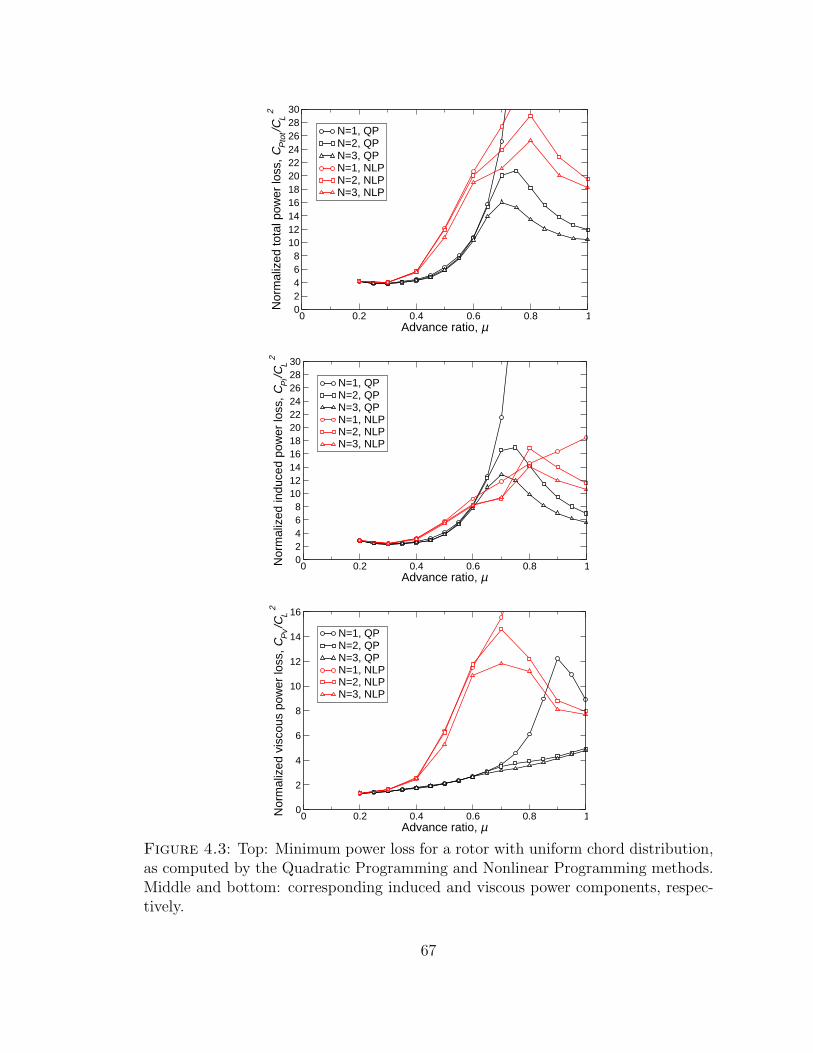
0 0.2 0.4 0.6 0.8 1Advance ratio, µ
02468
1012141618202224262830
Nor
mal
ized
tota
l pow
er lo
ss, C
Pto
t/CL
2
N=1, QPN=2, QPN=3, QPN=1, NLPN=2, NLPN=3, NLP
0 0.2 0.4 0.6 0.8 1Advance ratio, µ
02468
1012141618202224262830
Nor
mal
ized
indu
ced
pow
er lo
ss, C
Pi/C
L2
N=1, QPN=2, QPN=3, QPN=1, NLPN=2, NLPN=3, NLP
0 0.2 0.4 0.6 0.8 1Advance ratio, µ
0
2
4
6
8
10
12
14
16
Nor
mal
ized
vis
cous
pow
er lo
ss, C
Pv/C
L2
N=1, QPN=2, QPN=3, QPN=1, NLPN=2, NLPN=3, NLP
Figure 4.3: Top: Minimum power loss for a rotor with uniform chord distribution,as computed by the Quadratic Programming and Nonlinear Programming methods.Middle and bottom: corresponding induced and viscous power components, respec-tively.
67

low dynamic pressure in this region. Generating this large circulation requires large
effective angles of attack over a significant portion of the retreating side of the rotor,
particularly in the reverse flow region (ψ = 225 to ψ = 315, and at normalized
radial positions less than ≈ 0.4 in this case), where the blade sees large and rapidly
changing geometric angles of attack. The difference in the QP and NLP computed
circulation distributions is primarily located in this reverse flow region. However, as
we see in Figure 4.6, the µ = 0.4 radial twist and pitch input shown are quite similar
(though not identical) between the two methods, indicating that the two methods
have a very similar effective angles of attack at all locations in the wake. In the
reverse flow region, the assumption of a linear lift curve used in the QP method
results in a moderate, positive circulation, while the NLP solution has areas of zero
or negative circulation within this region. These differences in circulation result in
different induced powers for the two solutions.
At higher advance ratios, it becomes increasingly difficult to efficiently maintain
roll trim with N = 1 control, as investigated by Ormiston [27, 28, 29] and evidenced
by the rapid rise in induced power in both the the QP and NLP cases at advance ratios
above µ = 0.6. At these advance ratios, the QP solution is actually penalized by its
use of a linear lift curve, as the increasingly large cyclic pitch required at Ψ = 270
to maintain roll trim, shown in the bottom right plot of Figure 4.6, results in large
portions of the wake with very large magnitudes of circulation, resulting in high
induced power. The QP solution attempts to mitigate this by using a significantly
different radial twist distribution for the N = 1 solution, featuring a large positive
twist gradient from the root out to a normalized position of about 0.4. The differences
between the two solutions is further illustrated in Figure 4.5, which shows the NLP,
QP, and rubber rotor optimal circulation distributions at µ = 0.8. The QP solution
contains large levels of circulation throughout the wake, while the NLP and rubber
rotor solutions have significantly lower of values of circulation at all points. In this
68

case, the NLP solution benefits from the fact that its sectional coefficient of lift
is limited by stall, avoiding regions of excessively high circulation in the wake and
resulting in a lower induced power.
With the additional degrees of freedom available with N = 2 or N = 3 control,
the QP solution maintains trim without resorting to these excessively high angles
of attack, and the induced powers between the NLP and QP solutions are in better
(though still not perfect) agreement.
In summary, at low advance ratios (µ < 0.4), the results of the QP and NLP
methods are in fairly good agreement for the single rotor. The difference between the
QP and NLP results at high advance ratios is a result of the single rotor configuration
requiring very high coefficients of lift on the retreating side of the rotor. This leads to
azimuthal pitch inputs that feature large pitch angles and post-stall effective angles
of attack. The difference in how the two methods computes the coefficient of lift,
and ultimately circulation due to these large effective angles of attack, results in the
large differences in the power calculated by the two methods.
In a coaxial or wing-rotor configuration, maintaining trim at high advance ratios
does not require large root pitch inputs on the retreating side of the rotors. In fact,
the optimal solution for these configurations involves minimizing circulation and lift
in reverse flow regions. As a result, the QP and NLP results are in much better
agreement for these configurations, as we will see in Chapters 5 and 6. Additionally,
for a conventional rotor, the trends in total power with regard to increasing levels
of harmonic control are similar between the two methods, indicating that the QP
approach still provides some useful insight to the conventional rotor optimal control
problem at high advance ratios.
69

Figure 4.4: Optimal circulation distribution for a rotor at µ = 0.4. From left toright: NLP result and QP result with N = 1 root control, and rubber rotor solution.
Figure 4.5: Optimal circulation distribution for a conventional rotor at µ = 0.8.From left to right: NLP result and QP result with N = 1 root control, and rubberrotor solution.
4.3.2 Nonlinear Programming Results with Optimized Chord
The NLP results shown above account for realistic lift and drag curves and are
therefore more accurate than the QP results. All of the preceeding results use the
baseline chord distribution, which is a rectangular planform with a thrust weighted
solidity σTW = 0.1156. In this section, we include the chord distribution as a design
variable to be optimized, allowing the optimization algorithm to select the planform,
70
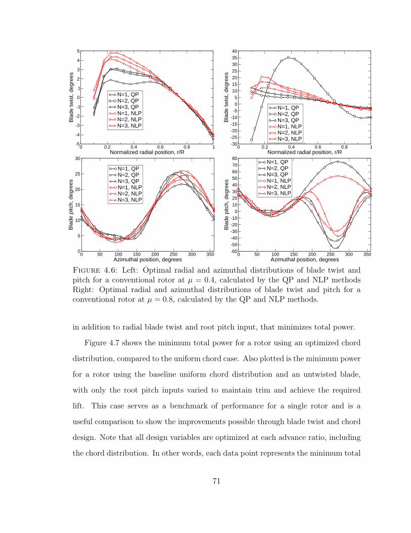
0 0.2 0.4 0.6 0.8 1Normalized radial position, r/R
-4
-2
0
2
4
3
1
-1
-3
-5
5
Bla
de tw
ist,
degr
ees
N=1, QPN=2, QPN=3, QPN=1, NLPN=2, NLPN=3, NLP
0 50 100 150 200 250 300 350Azimuthal position, degrees
0
10
15
20
25
5
30
Bla
de p
itch,
deg
rees
N=1, QPN=2, QPN=3, QPN=1, NLPN=2, NLPN=3, NLP
0 0.2 0.4 0.6 0.8 1Normalized radial position, r/R
-30-25-20-15-10-505
10152025303540
Bla
de tw
ist,
degr
ees
N=1, QPN=2, QPN=3, QPN=1, NLPN=2, NLPN=3, NLP
0 50 100 150 200 250 300 350Azimuthal position, degrees
-60-50-40-30-20-10
01020304050607080
Bla
de p
itch,
deg
rees
N=1, QPN=2, QPN=3, QPN=1, NLPN=2, NLPN=3, NLP
Figure 4.6: Left: Optimal radial and azimuthal distributions of blade twist andpitch for a conventional rotor at µ = 0.4, calculated by the QP and NLP methodsRight: Optimal radial and azimuthal distributions of blade twist and pitch for aconventional rotor at µ = 0.8, calculated by the QP and NLP methods.
in addition to radial blade twist and root pitch input, that minimizes total power.
Figure 4.7 shows the minimum total power for a rotor using an optimized chord
distribution, compared to the uniform chord case. Also plotted is the minimum power
for a rotor using the baseline uniform chord distribution and an untwisted blade,
with only the root pitch inputs varied to maintain trim and achieve the required
lift. This case serves as a benchmark of performance for a single rotor and is a
useful comparison to show the improvements possible through blade twist and chord
design. Note that all design variables are optimized at each advance ratio, including
the chord distribution. In other words, each data point represents the minimum total
71

power for a single point optimization at that specific advance ratio.
The optimized chord case achieves modest reductions in power at advance ratios
below µ = 0.4. Above this advance ratio, optimizing the chord results in large
reductions in power compared to the uniform chord case for all levels of harmonic
control. At µ = 0.8, the total power for the N = 1 case is reduced by 17% with
the use of an optimized chord distribution. Additionally, higher harmonic control
improves the performance among the optimized chord rotors, with N = 3 control
providing a 25% decrease in power relative to the N = 1 case. Of course, even with
higher harmonic control and a chord and twist distribution optimized only for fast
forward flight, the power requirements are still very high. The N = 3 optimized chord
case at µ = 0.8, which represents a value close to the lowest achievable power with
any blade root control scheme, corresponds to a lift over effective drag value below
4, which is still low relative to a fixed wing aircraft or the compound configurations
we will see in the following sections.
Figure 4.8 shows the radial twist and azimuthal pitch distribution for the opti-
mized chord case compared to the uniform chord case at an advance ratio of µ = 0.4.
Figure 4.9 shows the corresponding planform for the N = 1 and N = 3 optimized
chord cases. The optimal planform features a very unusual shape, with an extremely
small chord on its inner portion, a maximum chord at a normalized radial position
of 0.6, and then a rapid taper extending to the tip. The largest chord is nearly
twice as large as the baseline chord distribution. The thrust weighted solidity of the
optimal rotor is σTW = 0.132, compared to σTW = 0.116 for the baseline rotor. It
is somewhat surprising that the optimal viscous rotor planform has a higher solidity
and larger wetted surface area than the baseline constant chord case, which results
in higher viscous power. But in fact, at this advance ratio, the variable chord rotor
shape significantly reduces induced losses, more than the attendant increase in vis-
cous power. The influence of induced power on the solution will be explored further
72

0 0.2 0.4 0.6 0.8 1Advance ratio, µ
02468
10121416182022242628303234
Nor
mal
ized
tota
l pow
er lo
ss, C
Pto
t/CL
2 N=1, uniform chord and zero radial twistN=1, uniform chordN=2, uniform chordN=3, uniform chordN=1, optimized chordN=2, optimized chordN=3, optimized chord
Figure 4.7: Minimum power loss for a conventional rotor with chord optimizedcompared to a uniform chord case and a uniform chord and uniform twist case.
in the following section.
Lastly, Figure 4.10 shows the radial twist and azimuthal pitch distribution for the
optimized chord conventional rotor case at an advance ratio of µ = 0.8; Figure 4.11
shows the corresponding planforms. This is a fairly extreme flight condition, and
is not realistically attainable by conventional rotors. It is interesting, however, to
see the controls required to maintain trim at this high advance ratio. The N = 3
optimized chord case has a signficantly different root pitch input in the region from
ψ = 200 to ψ = 330 than the uniform chord case, although both achieve a similar
final effective angle of attack, albeit with the blade traversing through the flow in
the opposite direction, i.e. rotated by 180. The solidities of the optimal blades
are smaller at this high speed flight condition than in the µ = 0.4 case, as higher
dynamic pressures further penalize the large viscous drag resulting from a large
73

0 0.2 0.4 0.6 0.8 1Normalized radial position, r/R
-4
-2
0
2
4
6
8
10
12
14
Bla
de tw
ist,
degr
ees
N=1, optimized chordN=1, uniform chordN=3, optimized chordN=3, uniform chord
0 50 100 150 200 250 300 350Azimuthal position, degrees
0
10
15
20
25
5
30
Bla
de p
itch,
deg
rees
N=1, optimized chordN=1, uniform chordN=3, optimized chordN=3, uniform chord
Figure 4.8: Optimal radial and azimuthal distributions of blade twist and pitchfor a rotor with and without an optimized chord distribution, at µ = 0.4.
0 0.2 0.4 0.6 0.8 1r/R
-0.2
-0.1
0
0.1
x/R
Baseline, σTW
=0.116
N=1 , σTW
= 0.132
N=3, σTW
=0.129
Figure 4.9: Optimal blade planform at µ = 0.4 for varying levels of harmoniccontrol.
chord. Additionally, the N = 1 and N = 3 cases now have fundamentally different
planforms, with the majority of the blade area for the N = 1 case located near
the tip of the blade. The N = 3 case results in a more symmetric blade, with the
largest chord located approximately at midspan and without the excessively small
root chord values seen in the N = 1 case.
Figures 4.12 and 4.13 show the optimal circulation distribution and force distri-
bution, respectively, for the optimized chord cases. The solutions for the N = 1
case and the N = 3 case are shown, along with the rubber rotor solution. It is
interesting to note that at this high speed flight condition, nearly all of the lift is
being generated at the fore and aft positions of the rotor. This is a result of a ma-
74

0 0.2 0.4 0.6 0.8 1Normalized radial position, r/R
-8-6-4-202468
101214161820222426
Bla
de tw
ist,
degr
ees
N=1, optimized chordN=1, uniform chordN=3, optimized chordN=3, uniform chord
0 50 100 150 200 250 300 350Azimuthal position, degrees
-40
-20
0
20
40
60
80
100
120
140
Bla
de p
itch,
deg
rees
N=1, optimized chord N=1, uniform chordN=3, optimized chordN=3, uniform chord
Figure 4.10: Optimal radial and azimuthal distributions of blade twist and pitchfor a conventional rotor with and without an optimized chord distribution, at µ = 0.8.
0 0.2 0.4 0.6 0.8 1r/R
-0.2
-0.1
0
0.1
x/R
Baseline, σTW
=0.116
N=1, σTW
=0.114
N=3, σTW
=0.0872
Figure 4.11: Optimal blade planform at µ = 0.8 for varying levels of harmoniccontrol.
jority of the retreating wake having a low dynamic pressure, making it incapable of
generating significant lift. As a result, the advancing side must be almost entirely
offloaded to maintain roll trim. The force distribution is still skewed slightly towards
the advancing side, which must be balanced by a region of negative force at ψ = 90
in the N = 1 and N = 3 cases, leading to minimum powers much higher than the
rubber rotor optimal. The N = 3 case more closely matches the rubber rotor result
by decreasing the magnitude of the circulation at ψ = 0 and ψ = 180 and generat-
ing a region of negative circulation in the reverse flow region between ψ = 270 and
ψ = 330.
75

Figure 4.12: Optimal circulation distribution for a rotor with optimized chord atµ = 0.8. From left to right: N = 1 control, N = 3 control, and rubber rotor solution.
Figure 4.13: Optimal force per span distribution for a rotor with optimized chordat µ = 0.8. From left to right: N = 1 control, N = 3 control, and rubber rotorsolution.
4.3.3 Comparison of Viscous Optimum to Inviscid Optimum
The previous sections showed the results of viscous optimizations, or optimizations
that sought to minimize the sum of induced and viscous power. It is interesting to
examine the inviscid solution, which minimizes only induced power, to see how it
compares to the viscous solution. First, Table 4.1 shows a comparison of the inviscid
and viscous minimum powers at µ = 0.4 using N = 1 and N = 3 control. Note
that although the inviscid optimizations were performed without regard to viscous
76

power, a viscous power associated with the optimal solution can still be computed.
As expected, for both N = 1 and N = 3 control, the inviscid optimum has a lower
induced power (CPi/C2L), than the viscous optimum (of course this has to be the
case, or the viscous optimum would in fact be the inviscid optimum). Similarly, the
viscous optimum has a lower total power than the inviscid case. It is interesting to
note that the induced power for the viscous optimizations is very close (within about
10%) to the induced minimum power. The viscous solution is able to trade some
of this induced power for further decreases in viscous power, resulting in a lower
total power. Also of interest, the lower total power associated with N = 3 control is
entirely a result of reductions in induced power, as the viscous powers of the N = 1
and N = 3 cases are identical. More generally, the N = 3 case is only slightly better
than the N = 1 case for the viscous analysis.
Table 4.1: Induced, viscous, and total power at µ = 0.4 for inviscid and viscousoptimal solutions of single rotor.
N=1 N=3Inviscid Viscous Inviscid Viscousdesign design design design
Induced power, CPi/C2L 2.52 2.68 2.35 2.62
Viscous power, CPv/C2L 2.97 2.40 3.17 2.40
Total power, CPtot/C2L 5.49 5.08 5.52 5.03
The optimal circulation distribution for each solution is shown in Figure 4.14. The
two distinct optimizations have a nearly identical circulation distribution, reinforcing
the fact that induced losses are a significant driver in the total power optimum, even
in cases featuring an optimized chord. Figure 4.15 shows the inviscid versus viscous
radial twist and azimuthal pitch input for µ = 0.4. Both the inviscid and viscous
solutions are very similar.
The effect of induced losses on optimal planform shape can be seen by examining
77

Figure 4.14: Optimal circulation distribution for a rotor with N = 1 control andan optimized chord distribution at µ = 0.4. Left: Viscous solution. Right: Inviscidsolution.
the optimal inviscid rotor planform shown in Figure 4.16. Note that for the inviscid
case, the planform has the same general shape, but with a slightly higher solidity.
The optimized viscous planform, as one might expect, has a slightly smaller wetted
surface area than the inviscid case, although as discussed previously, it is still larger
than the baseline rotor.
0 0.2 0.4 0.6 0.8 1Normalized radial position, r/R
-2
0
2
4
6
8
10
12
14
16
18
20
22
Bla
de tw
ist,
degr
ees
N=1, viscousN=1, inviscidN=3, viscousN=3, inviscid
0 50 100 150 200 250 300 350Azimuthal position, degrees
0
10
15
20
25
5
Bla
de p
itch,
deg
rees
N=1, viscousN=1, inviscidN=3, viscousN=3, inviscid
Figure 4.15: Comparison of inviscid and viscous radial and azimuthal distributionsof blade twist and pitch for a rotor using N = 1 and N = 3 control at µ = 0.4
78

0 0.2 0.4 0.6 0.8 1r/R
-0.2
-0.1
0
x/R
Baseline, σTW
= 0.116
N=1 viscous, σTW
= 0.132
N=1 inviscid, σTW
=0.199
Figure 4.16: Comparison of inviscid and viscous optimal planforms at µ = 0.4 fora rotor using N = 1 control.
4.4 Conclusions from Analysis of a Conventional rotor
Based on the analysis of a conventional rotor using higher harmonic control in this
chapter, we can draw the following specific conclusions
1. The quadratic programming method is computationally fast, requiring only
several minutes of CPU time on a desktop computer for each flight condition.
At advance ratios below about µ = 0.4, the quadratic programming method
produces a solution that is very close to the more accurate nonlinear program-
ming method. At advance ratios above µ = 0.4, the two methods arrive at
similar radial twist and azimuthal pitch solutions, but compute significantly
different induced, viscous and total powers. This is a result of the large effec-
tive angles of attack required on the retreating side of the rotor to maintain
roll trim.
2. Despite the differences in the results at high advance ratios, the general trends
with respect to advance ratio, level of harmonic control, and basic radial and
azimuthal pitch inputs are similar between the QP and NLP methods, indicat-
ing that the QP method is still of use in the analysis of a single rotor despite
its simplifying assumptions. Additionally, at advance ratios below µ = 0.4, the
79

QP and NLP methods are in close agreement.
3. For the uniform chord case, the use of higher harmonic control produces large
decreases in total power, with N = 2 and N = 3 control offering reductions of
19% and 42%, respectively, compared to N = 1 control at µ = 0.8. At lower
advance ratios typical of a conventional rotor, the reduction in power is more
modest, on the order of 2%.
4. Use of an optimized chord distribution also provides large reductions in power
at both low and high advance ratios. For N = 1 control, use of an optimized
chord distribution results in an 11% reduction in total power at µ = 0.4 and a
17% reduction in total power at µ = 0.8. The optimal planform in the µ = 0.4
case has a higher solidity than the baseline rotor, with a large chord near the
midspan of the blade which tapers towards the root and tip.
5. Higher harmonic control is effective in reducing power at high advance ratios
when used in conjuction with an optimized chord distribution. For example,
use of N = 3 control with optimized chord provides a 25% reduction in power
compared to the N = 1 optimized chord case at µ = 0.8.
6. The viscous minimum power solution is driven by induced losses, as the optimal
inviscid and viscous circulation distributions and radial twist and azimuthal
pitch inputs are very similar. This fact is supported by both the theory (the
generalized Betz criterion) and the numerical results.
80

5
Coaxial Rotor Results
In this chapter, we analyze the optimal performance of a coaxial, counter-rotating
rotor system. The contour plots displayed in this chapter will include representations
of both the upper and lower rotor in body-fixed coordinates. In all contour plots,
the vehicle is traveling up the page, with the upper rotor rotating counter-clockwise
and the lower rotor rotating clockwise. As a result, the advancing side is the right
half of the upper rotor and the left half of the lower rotor.
5.1 Baseline Rotor
The parameters selected for this configuration were meant to closely resemble the
Sikorsky X2 Technology Demonstrator, shown in Figure 1.4.
We consider a system of two coaxial counterrotating rotors. We analyze rotors
similar to the design intent of the X2 rotor system in high speed cruise as described
by Bagai [5]. The design intent advance ratio, µ, is 0.85; the thrust weighted solidity,
σTW, is 0.1441, and the modified thrust weighted solidity as defined in Equation 3.64,
σTWM, is 0.116; the coefficient of lift, CL, is 0.02324 corresponding to a CL/σTW of
0.1613; and the relative tip Mach number is 0.9. The rotors have no coning, and the
81

shaft is tilted nose down at an angle of αshaft = −5. We use a root cutout equal
to 10 percent of the rotor radius, with a vertical spacing between the rotors equal to
20 percent of the rotor radius. Both the upper and lower rotors are constrained to
use the same fixed radial blade twist and chord; however, each rotor has its own set
of root pitch inputs.
In all cases, we require the total rotor system to be in moment trim; the moments
on an individual rotor may be nonzero as long as the net moment is zero, requiring
that the rotors be rigid. As a result, each rotor will carry an offset lift on the
advancing side of the rotor.
To analyze these cases, we use the methods described in Chapters 2 and 3 with
a lattice of vortex rings containing 18 elements in the spanwise direction and 15
elements in the azimuthal direction for each of the eight rotor blades, for a total of
2160 vortex ring elements.
5.2 Quadratic Programming Results
In this section, we present solutions to the optimal blade control problem for the
baseline rotor with fixed chord, varying radial twist, a quadratic drag polar, and
linearized lifting line theory. We assume a uniform chord that gives the modified
thrust weighted solidity of the X2 design. Although the relative tip Mach number of
the X2 design varies from approximately 0.65 to 0.9 over the range of advance ratios
from 0.2 to 1.0 [5], for simplicity we maintain Mtip = 0.9 over all advance ratios.
Although Mach number has some effect on the optimal controls, it has a minimal
effect on power requirements, and the simplification of a uniform Mtip does not result
in large changes in the optimal solution. The airfoil sectional lift curve slope is equal
to 2π, and the NACA 0012 quadratic drag polar shown in Figure 2.3 is used.
Figure 5.1 shows the computed minimum total, induced, and profile power losses
for varying levels of blade root harmonic control over a range of advance ratios. At
82

0 0.2 0.4 0.6 0.8 1Advance ratio, µ
0
0.5
1.0
1.5
2.0
2.5
3.0
Nor
mal
ized
tota
l pow
er lo
ss, C
Pto
t/CL
2
N=1N=2N=3N=10Rubber rotor
0 0.2 0.4 0.6 0.8 1Advance ratio, µ
0
0.5
1.0
1.5
2.0
2.5
3.0
Nor
mal
ized
indu
ced
pow
er lo
ss, C
Pi/C
L2
N=1N=2N=3N=10Rubber rotor
0 0.2 0.4 0.6 0.8 1Advance ratio, µ
0
0.5
1.0
1.5
Nor
mal
ized
vis
cous
pow
er lo
ss, C
Pv/C
L2
N=1N=2N=3N=10Rubber rotor
Figure 5.1: Top: Minimum power loss for a coaxial rotor in trimmed forwardflight with varying levels of blade root harmonic control. Middle and bottom: cor-responding induced and viscous power components, respectively. All results use theQuadratic Programming method.
83

each advance ratio, all design variables, including the fixed radial twist, are opti-
mized. Also shown is the rubber rotor minimum power, i.e. the absolute minimum
power achievable within this rotor configuration assuming infinite degrees of free-
dom in blade articulation. For advance ratios less than about 0.5, higher harmonic
control does not provide a significant reduction in power. For higher advance ratios,
however, the total power required is dramatically reduced with diminishing returns
for N greater than three. At the design advance ratio of µ = 0.85, higher harmonic
control can reduce the total power required by about 20%. As in the single rotor
case, the minimum power solution does not asymptote to the rubber rotor optimum,
even with high levels of blade root harmonic control, because of the lack of radial
twist control as a function of azimuth. Furthermore, almost all of the decrease in to-
tal power is a result of improvements in the induced power of the rotor. The viscous
power losses are nearly identical for all levels of harmonic control.
Figure 5.2 shows the optimal fixed blade twist at advance ratios of µ = 0.5 and
µ = 0.85 for varying levels of harmonic control. Also shown is the blade pitch control
as a function of azimuth. The azimuthal angle is positive in the direction of each of
the rotors’ rotation, so here azimuth represents advancing time. The blade pitch is
nearly the same for the upper and lower rotors, with a slight asymmetry caused by
the −5 tilt of the shaft.
For the µ = 0.85 case, note the very interesting azimuthal variation of blade root
pitch in both the N = 2 and N = 10 higher harmonic control schemes. The twist
is abruptly reduced by about 25 degrees at ψ ≈ 225, with a corresponding increase
at ψ ≈ 310. This dropoff in pitch angle takes place in the portion of the rotor
disk where the blade enters and exits the reverse flow region. To understand this
behavior, the optimal circulation on the rotor disk for N = 1 and N = 10 is plotted
in Figure 5.3, and also for the rubber rotor. Note that the N = 1 solution has a
region of positive circulation on the retreating sides of the upper and lower rotors, a
84

feature not present in the rubber rotor. The circulation in this region is dramatically
reduced in the N = 10 solution by reducing the pitch of the blade as it sweeps
through this region, resulting in lower induced and total power. The N = 1 control
scheme does not have the level of azimuthal control necessary to achieve this abrupt
reduction in pitch, and instead compensates by using a significantly decreased level
of fixed blade twist on the inboard portion of the blade, a method not as effective
at mitigating the circulation in the reverse flow region, leading to the N = 1 case
having significantly higher induced and total powers than the N = 2 and higher
cases.
0 0.1 0.2 0.3 0.4 0.5 0.6 0.7 0.8 0.9 1
Normalized radial position, r/R
-5
-4
-3
-2
-1
0
1
2
3
4
5
-6
Bla
de tw
ist,
degr
ees
N=1N=2N=10
0 50 100 150 200 250 300 350
Azimuthal position, degrees
0
10
15
20
25
5
-5
-10
-15
-20
Bla
de p
itch,
deg
rees
N=1, upper rotorN=1, lower rotorN=2, upper rotorN=2, lower rotorN=10, upper rotorN=10, lower rotor
Figure 5.2: Left: Optimal radial and azimuthal distributions of blade twist andpitch for coaxial rotors at µ = 0.5. Right: Optimal radial and azimuthal distributionsof blade twist and pitch for coaxial rotors at µ = 0.85.
Figure 5.4 shows the optimal force per span distribution on the rotor. For both
85

Figure 5.3: Optimal circulation distribution on upper and lower rotors of a coaxialsystem at µ = 0.85, computed by QP method. Left: N = 1 control. Middle: N = 10control. Right: Rubber rotor.
N = 1 and N = 10 control and the rubber rotor case, nearly all of the force is gener-
ated on the advancing side of the rotor, where dynamic pressures are high, allowing
much of the retreating blade to be offloaded. The region of positive circulation on
the retreating side of the N = 1 solution results in a small region of force on the
retreating side, a feature that adds to the total power and is not seen in the N = 10
and rubber rotor solutions.
Figure 5.4: Optimal force distribution on upper and lower rotors of a coaxialsystem at µ = 0.85, computed by QP method. Left: N = 1 control. Middle: N = 10control. Right: Rubber rotor.
86
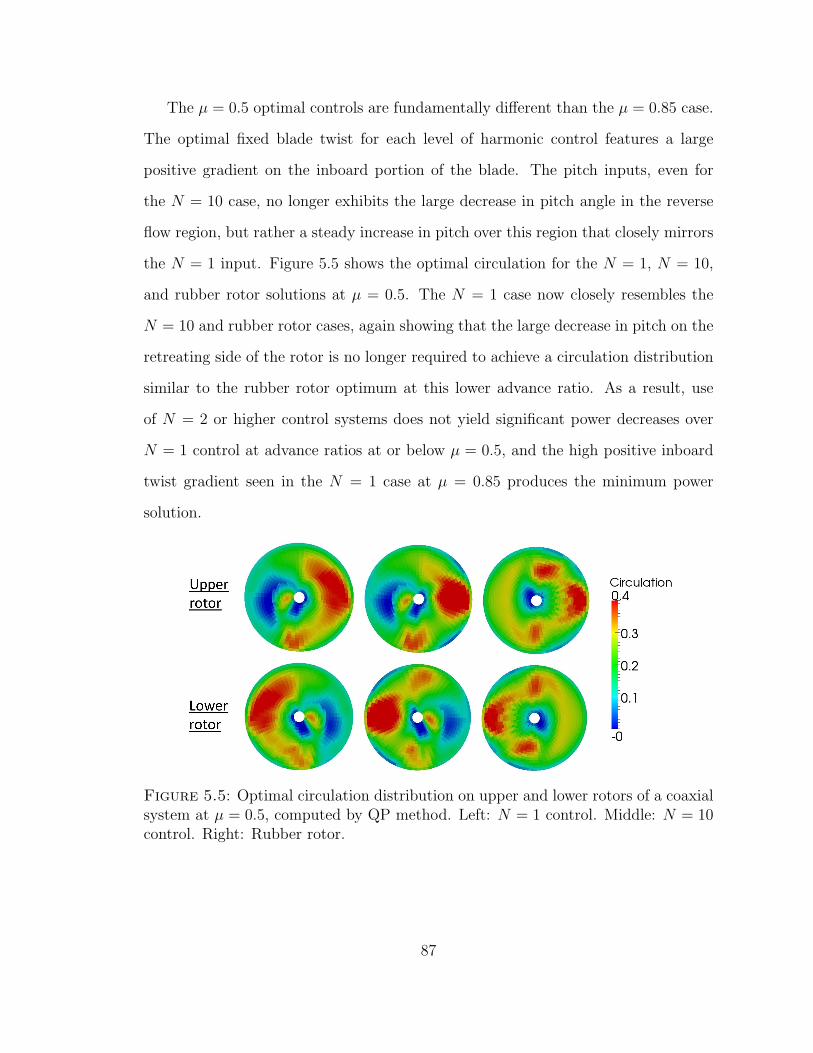
The µ = 0.5 optimal controls are fundamentally different than the µ = 0.85 case.
The optimal fixed blade twist for each level of harmonic control features a large
positive gradient on the inboard portion of the blade. The pitch inputs, even for
the N = 10 case, no longer exhibits the large decrease in pitch angle in the reverse
flow region, but rather a steady increase in pitch over this region that closely mirrors
the N = 1 input. Figure 5.5 shows the optimal circulation for the N = 1, N = 10,
and rubber rotor solutions at µ = 0.5. The N = 1 case now closely resembles the
N = 10 and rubber rotor cases, again showing that the large decrease in pitch on the
retreating side of the rotor is no longer required to achieve a circulation distribution
similar to the rubber rotor optimum at this lower advance ratio. As a result, use
of N = 2 or higher control systems does not yield significant power decreases over
N = 1 control at advance ratios at or below µ = 0.5, and the high positive inboard
twist gradient seen in the N = 1 case at µ = 0.85 produces the minimum power
solution.
Figure 5.5: Optimal circulation distribution on upper and lower rotors of a coaxialsystem at µ = 0.5, computed by QP method. Left: N = 1 control. Middle: N = 10control. Right: Rubber rotor.
87

5.3 Nonlinear Programming Results
In this section, we present solutions to the nonlinear optimal blade control problem
for the baseline coaxial configuration. The full nonlinear problem accounts for a
nonlinear lift curve, including stall, a non-quadratic drag polar, does not assume
small induced angles of attack, and is capable of optimizing the chord distribution
in addition to other design variables. The blade analyzed uses a NACA0012 airfoil
from root to tip, with data of the coefficient of lift and drag through the full range of
angles of attack obtained from Reference [39]. Again, the coefficient of lift is modified
by Mach number using the Prandtl-Glauert transform, and the coefficient of drag is
unchanged. All advance ratios are analyzed assuming a relative Mach number of 0.9.
5.3.1 Comparison of Nonlinear Programming Results to Quadratic ProgrammingResults
First, we compare the nonlinear programming results (NLP) for a uniform chord
distribution to the Quadratic Programming results shown in the preceeding sec-
tion. The QP approach is extremely efficient, capable of solving the optimal controls
problem for a single advance ratio in about 10 minutes on a single processor machine
compared to several hours for the NLP problem. To make a direct comparison of
the two methods, the chord distribution is not included as a design variable to be
optimized in the following NLP results. Thus, both the NLP and QP solutions will
have the same uniform blade planform.
Figure 5.6 shows the minimum total, induced, and profile power losses for varying
levels of blade root harmonic control over a range of advance ratios for a uniform
chord distribution, as computed by each approach. The NLP results are shown
in red, with the QP results in black. The QP and NLP results are very much in
agreement, particularly at low advance ratios. The QP method tends to slightly
underpredict the viscous power loss, particularly for the N = 1 case. This is a result
88

of using the quadratic drag polar, which underpredicts the coefficient of drag at
angles of attack beyond stall, resulting in a lower profile power loss. The minimum
induced power losses are also very similar between the two approaches, again with
excellent agreement at low advance ratios. For every level of harmonic control across
all advance ratios, the QP result slightly underpredicts the total power loss of the
NLP result. It is encouraging, however, that the QP and NLP results all follow the
same trends and are in general very close to one another.
It is useful to compare the design variables predicted by the two methods, in
addition to the minimum powers, to ensure that the two methods don’t lead to
fundamentally different control inputs. Figure 5.7 shows the optimal fixed blade
twist and root pitch input at an advance ratio of µ = 0.85 computed by the QP and
NLP approaches. The optimal controls are very similar between the two methods.
Part of the reason the QP method gives good results is that its primary assump-
tions of a linear lift curve, quadratic drag polar, and small induced angles of attack
are reasonable when the blade is operating at small effective angles of attack (i.e.
unstalled). These assumptions are less accurate in the reverse flow region of the
wake, where geometric angles of attack can be large, leading to large effective and
induced angles of attack. In the conventional rotor result, large effective angles of
attack are required in the reverse flow region, and in fact on the entire retreating
side of the disk, to provide lift to maintain roll trim at high advance ratios. As
a result, the optimal controls feature large portions of the blade operating in the
stalled regime, leading to significant differences between the QP and NLP results
at these high advance ratios. In contrast, the coaxial rotor solution minimizes the
circulation in the reverse flow region, and does not require significant lift generation
on the retreating side of the rotor. As a result, the optimal coaxial solution does not
rely on large angles of attack to maintain roll trim, and the QP and NLP optimum
controls and minimum powers are in very good agreement.
89

0 0.2 0.4 0.6 0.8 1Advance ratio, µ
0
0.5
1.0
1.5
2.0
2.5
3.0
Nor
mal
ized
tota
l pow
er lo
ss, C
Pto
t/CL
2
N=1, QPN=2, QPN=3, QPN=1, NLPN=2, NLPN=3, NLP
0 0.2 0.4 0.6 0.8 1Advance ratio, µ
0
0.5
1.0
1.5
2.0
2.5
Nor
mal
ized
indu
ced
pow
er lo
ss, C
Pi/C
L2
N=1, QPN=2, QPN=3, QPN=1, NLPN=2, NLPN=3, NLP
0 0.2 0.4 0.6 0.8 1Advance ratio, µ
0
0.5
1.0
1.5
2.0
Nor
mal
ized
vis
cous
pow
er lo
ss, C
Pv/C
L2
N=1, QPN=2, QPN=3, QPN=1, NLPN=2, NLPN=3, NLP
Figure 5.6: Top: Minimum power loss for a coaxial rotor with uniform chord dis-tribution, as computed by the Quadratic Programming and Nonlinear Programmingmethods. Middle and bottom: corresponding induced and viscous power compo-nents, respectively.
90

Figure 5.8 shows the optimal circulation distributions for the QP and NLP results
at µ = 0.85. The similarity between the two results reaffirms the accuracy of the
QP method. As might be expected, the only significant discrepancy occurs in the
reverse flow region, where the QP result computes a higher circulation than the NLP
result due to its use of a linear lift curve, resulting in unrealistically high coefficients
of lift at these high angles of attack. The QP result is further helped by the fact
that the reverse flow region has a low dynamic pressure, resulting in the circulation
generated in this region having a relatively small effect on the total calculated power
and forces. In summary, the QP method is an extremely useful tool to efficiently
compute optimal coaxial rotor design over a range of advance ratios.
0 0.1 0.2 0.3 0.4 0.5 0.6 0.7 0.8 0.9 1
Normalized radial position, r/R
-5
-4
-3
-2
-1
0
1
2
3
4
-6
-7
Bla
de tw
ist,
degr
ees
N=1, QPN=2, QPN=3, QPN=1, NLPN=2, NLPN=3, NLP
0 50 100 150 200 250 300 350
Azimuthal position, degrees
0
10
15
20
5
-5
-10
-15
-20
-25
Bla
de p
itch,
deg
rees
N=1, QPN=2, QPN=3, QPN=1, NLPN=2, NLPN=3, NLP
Figure 5.7: Optimal radial and azimuthal distributions of blade twist and pitch forcoaxial rotors with varying levels of harmonic control at µ = 0.85, with QP resultscompared to the Newton iteration results with a uniform chord.
5.3.2 Nonlinear Programming Results with Optimized Chord
The primary benefit of the nonlinear approach for the coaxial configuration then,
apart from some marginal improvement in accuracy over the QP method, is the
ability to optimize the chord distribution. In this section, we examine the improve-
ments that can be gained by tailoring the chord distribution with and without higher
harmonic control.
91

Figure 5.8: Optimal circulation distribution for a coaxial rotor with N = 1 controlat µ = 0.85, as computed by the QP and NLP methods. Left: QP solution. Right:NLP solution.
For each of the optimized chord cases, the modified thrust weighted solidity is
constrained to be the same as the X2 technology demonstrator, σTWM = 0.116. If
the rotor’s solidity is left unconstrained, the optimal rotor for high advance ratios
has excessively small blade areas. This is because the high dynamic pressures on
the advancing side of each rotor do not require very much blade area to generate the
required lift, and small chord values minimize profile losses and lift generation in sub-
optimal locations. While very efficient in forward flight, this solution is not practical
in hover and is therefore of limited interest. Implementing a solidity constraint
ensures an adequate blade area for flight in all regimes, including hover.
We choose to constrain the modified thrust weighted solidity, rather than the tra-
ditional thrust weighted solidity. Because the thrust weighted solidity heavily weights
chord at the blade tip, and because the circulation goes to zero at the tip regardless
of the chord, we found that a constraint on thrust weighted solidity produced oddly
shaped tip geometries. To alleviate this problem, we constrain instead the modified
thrust weighted solidity defined by Equation 3.64, allowing the optimization to select
the most advantageous tip shape for aerodynamic performance.
92

The minimum blade chord is constrained to be 1% of the rotor radius, to ensure
the chord distribution does not assume a negative value at any point along the span.
While this very small blade chord would likely not meet structural requirements for
the blade, this case is still of interest, as it gives the most aerodynamically efficient
rotor design at this speed, and when used in addition to the solidity constraint,
ensures sufficient blade area for the vehicle to hover. A case with a higher minimum
chord constraint that more accurately reflects the actual design of a blade is given
in Section 5.3.6.
Figure 5.9 shows the minimum total power over a range of advance ratios and
levels of harmonic control for the coaxial rotor, with all control inputs and design
variables optimized at each advance ratio. Also plotted in Figure 5.9 is the mini-
mum total power for the coaxial rotor with a uniform chord distribution, which has
the same solidity (σTWM = 0.116) as each optimized chord case. Additionally, the
minimum total power for a rotor using N = 1 control, a uniform chord distribution,
and a blade with no radial blade twist (i.e., an untwisted rectangular blade where
only the root inputs are optimized) is also plotted. This serves as a benchmark of
performance for the coaxial rotor if the twist, chord, and higher harmonic control
design variables are not utilized.
For a given level of harmonic control, optimizing the chord distribution provides
power reductions over the uniform chord case at all advance ratios. At the design
point of µ = 0.85, the N = 1 case with an optimized chord distribution results in a
16% reduction in total power compared to the uniform chord case. This reduction in
power is achieved primarily through a reduction in induced power, although profile
power losses are also decreased. Use of N = 3 control with an optimized chord results
in an additional 16% reduction in power compared to the N = 1 control case with
an optimized chord, showing that even with an optimized chord, higher harmonic
control still produces substantial benefits.
93

0 0.2 0.4 0.6 0.8 1Advance ratio, µ
0
0.5
1.0
1.5
2.0
2.5
3.0
3.5
Nor
mal
ized
tota
l pow
er lo
ss, C
Pto
t/CL
2
N=1, uniform chord and zero radial twistN=1, uniform chordN=2, uniform chordN=3, uniform chordN=1, optimized chordN=2, optimized chordN=3, optimized chord
Figure 5.9: Minimum power loss for a coaxial rotor with chord optimized comparedto a uniform chord case and a uniform chord and uniform twist case.
Figure 5.10 shows the optimal radial twist and pitch input for the optimized chord
case at µ = 0.85, as well as the optimal pitch input for the N = 1 uniform chord case.
Note that because the pitch input for the upper and lower rotors are so similar, for
simplicity only the upper rotor pitch input is plotted. Figure 5.11 shows the optimal
planform for N = 1 and N = 3 control, in addition to the baseline uniform chord
distribution. As in the uniform chord case, the N = 1 case uses a large positive
twist gradient on the inboard section of the blade at high advance ratios, in addition
to a very small chord at the root. Both the small chord and positive twist gradient
serve to decrease the circulation generated in the reverse flow region, resulting in a
circulation distribution that more closely resembles the rubber rotor optimum. For
the N = 2 and N = 3 cases, it is optimal to have more of the blade area inboard, and
use the extra degrees of freedom in the root pitch input to decrease pitch angle and
94

minimize circulation on the retreating side. Also of note, the N = 1 pitch control for
the optimized chord case has switched phase compared to the uniform chord case.
For the optimized chord case, cyclic control is no longer providing roll trim, because
the coaxial counterrotating rotor is naturally trimmed. Instead, the cyclic control
here improves the performance primarily by reducing induced power.
Figure 5.12 shows the circulation distributions for the N = 1 fixed and optimized
chord cases, the N = 3 optimized chord case, and the rubber solution. Looking
at the two N = 1 cases shows the differences in the circulation distribution simply
as a result of optimizing the planform – the positive region of circulation on the
retreating side of each rotor is no longer present, due to the small inboard chord
distributions, and the region of positive circulation on the advancing side is reduced,
more closely resembling the rubber rotor optimum. Using N = 3 control with the
optimized chord results in further improvements, with the circulation distribution
further approaching the rubber rotor optimal.
0 0.1 0.2 0.3 0.4 0.5 0.6 0.7 0.8 0.9 1
Normalized radial position, r/R
-2
-1
0
1
2
3
4
5
6
7
8
9
10
Bla
de tw
ist,
degr
ees
N=1, optimized chordN=2, optimized chordN=3, optimized chord
0 50 100 150 200 250 300 350
Azimuthal position, degrees
0
10
15
20
5
-5
-10
-15
-20
-25
Bla
de p
itch,
deg
rees
N=1, optimized chordN=2, optimized chordN=3, optimized chordN=1, uniform chord
Figure 5.10: Optimal radial and azimuthal distributions of blade twist and pitchfor coaxial rotors with varying levels of harmonic control and chord optimized atµ = 0.85.
Lastly, Figure 5.13 shows how the optimal blade planform varies with advance
ratio for theN = 1 case. At low advance ratios, it is optimal to have more of the blade
area inboard. This results in higher total blade area, as the inboard chord is weighted
95
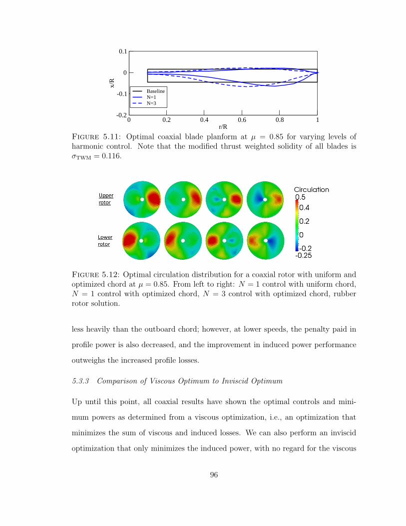
0 0.2 0.4 0.6 0.8 1r/R
-0.2
-0.1
0
0.1
x/R
BaselineN=1N=3
Figure 5.11: Optimal coaxial blade planform at µ = 0.85 for varying levels ofharmonic control. Note that the modified thrust weighted solidity of all blades isσTWM = 0.116.
Figure 5.12: Optimal circulation distribution for a coaxial rotor with uniform andoptimized chord at µ = 0.85. From left to right: N = 1 control with uniform chord,N = 1 control with optimized chord, N = 3 control with optimized chord, rubberrotor solution.
less heavily than the outboard chord; however, at lower speeds, the penalty paid in
profile power is also decreased, and the improvement in induced power performance
outweighs the increased profile losses.
5.3.3 Comparison of Viscous Optimum to Inviscid Optimum
Up until this point, all coaxial results have shown the optimal controls and mini-
mum powers as determined from a viscous optimization, i.e., an optimization that
minimizes the sum of viscous and induced losses. We can also perform an inviscid
optimization that only minimizes the induced power, with no regard for the viscous
96

0 0.2 0.4 0.6 0.8 1r/R
-0.2
-0.1
0
0.1
x/R
N=1, µ=0.2N=1, µ = 0.5N=1, µ=0.85
Figure 5.13: Optimal coaxial blade planform at varying advance ratios for N = 1harmonic control.
losses. While minimizing viscous losses on a rotor involves decreasing blade area
and ensuring that airfoils operate at angles of attack where they have a high ratio
of lift to drag, it is not as clear what design features make up the minimum induced
loss solution. As a result, it is interesting to look at the completely inviscid solution
with no regard to viscous losses, and compare this to the viscous optimization that
accounts for both these induced losses and viscous effects.
First, we examine the minimum powers from each of these optimizations at the
design point of µ = 0.85, shown in Table 5.1. These cases optimized both chord
and twist for N = 1, N = 2, and N = 3 harmonic control. Note that although the
inviscid optimization does not account for viscous effects in determining the optimal
control inputs, the viscous power loss associated with these controls can still be
computed, to give the inviscid solution a viscous and total power. First note that
for the inviscid optimization, higher harmonic control results in decreased induced
power (CPi/C2L), while for the viscous solution, higher harmonic control results in
decreased total power (CPtot/C2L) It is interesting to see how the viscous solution
achieves this reduction in total power with the use of higher harmonic control. The
N = 2 viscous solution improves total power through decreases in viscous power;
in fact, the inviscid power is actually slightly higher for the N = 2 solution than
the N = 1 solution. The N = 3 viscous solution is able to substantially reduce
97

Table 5.1: Induced, viscous, and total power at µ = 0.85 for coaxial rotor at inviscidand viscous optimal solutions.
N=1 N=2 N=3Inviscid Viscous Inviscid Viscous Inviscid Viscousdesign design design design design design
Induced power, CPi/C2L 1.11 1.19 1.05 1.20 1.00 1.04
Viscous power, CPv/C2L 1.26 0.97 1.75 0.76 1.15 0.77
Total power, CPtot/C2L 2.38 2.15 2.81 1.96 2.15 1.81
induced power over the N = 2 solution while maintaining the same viscous losses.
At N = 3, the induced power for the viscous solution, 1.04, is very close to the
minimum induced power, 1.00. In fact, the viscous optimization is within 15% of
the minimum induced power loss at all levels of harmonic controls, indicating that
minimizing induced power losses is a key driver in minimizing total power.
The fact that induced losses dominate the viscous optimization is also reflected
in Figure 5.14, which shows the optimal radial pitch and root pitch input for the
inviscid and viscous solutions using N = 1 and N = 3 control at the design point
of µ = 0.85. In all cases, both the blade twist and blade chord are optimized. The
inviscid radial blade twist is very similar to the viscous solution, with the exception of
the behavior at the tip of the blade, where the viscous solution has a large positive
twist gradient. The root pitch inputs are also very similar between the viscous
and inviscid solutions, however the inviscid inputs tend to “exaggerate” the same
features seen in the viscous solutions. For example, the N = 3 inviscid solution has
a significantly larger decrease in pitch angle between ψ = 230 and ψ = 330 than the
viscous solution. The inviscid solution is able to achieve slightly lower induced powers
by using this large negative blade pitch, reducing circulation in this region. However,
the resultant large angles of attack seen on some portions of the blade result in blade
stall and high coefficients of drag, as evidenced by the fact that the inviscid solution
98

has nearly 50% higher viscous drag then the viscous solution. The viscous solution
uses a slightly less drastic dip in pitch angle, trading a small increase in induced
power for a large decrease in viscous power to locate the minimum total power. This
similarity in the controls results in nearly identical circulation distributions between
the inviscid and viscous solutions, as shown in Figure 5.15 for the N = 1 case. The
viscous solution has slightly exagerrated regions of circulation, resulting in slightly
higher induced powers; however, this tradeoff induced power results in a decrease in
viscous power and a net reduction in total power.
0 0.1 0.2 0.3 0.4 0.5 0.6 0.7 0.8 0.9 1
Normalized radial position, r/R
-3
-2
-1
0
1
2
3
4
5
6
7
8
9
10
11
12
Bla
de tw
ist,
degr
ees
N=1, inviscid optimizationN=1, viscous optimizationN=3, inviscid optimizationN=3, viscous optimization
0 50 100 150 200 250 300 350
Azimuthal position, degrees
0
10
15
20
5
-5
-10
-15
-20
-25
-30
-35
-40
-45
-50
Bla
de p
itch,
deg
rees
N=1, inviscid optimizationN=1, viscous optimizationN=3, inviscid optimizationN=3, viscous optimization
Figure 5.14: Comparison of inviscid and viscous radial and azimuthal distributionsof blade twist and pitch for N = 1 and N = 3 control at µ = 0.85.
Figure 5.16 shows the optimal blade planforms for the N = 1 and N = 3 inviscid
and viscous optimizations at the design point. Similar to the radial blade twist
distributions, the N = 1 viscous and inviscid solutions have remarkably similar
planforms with the exception of the blade tip. The viscous optimum has a drastically
reduced tip chord, a feature that makes sense given the high dynamic pressure at the
tip and the minimal impact on the induced power that this region has, given that the
circulation goes to zero at the tip regardless of blade geometry. The N = 3 inviscid
case does not have the large tip chord seen in the N = 1 case. As a result, for N = 3
control, the inviscid and viscous solutions have a nearly identical planform.
99

Figure 5.15: Optimal circulation distribution for a coaxial rotor with optimizedchord and N = 1 control at µ = 0.85 Left: Inviscid solution. Right: Viscous solution.
0 0.2 0.4 0.6 0.8 1r/R
-0.2
-0.1
0
0.1
x/R
N=1, viscous optimizationN=1, inviscid optimization
0 0.2 0.4 0.6 0.8 1r/R
-0.2
-0.1
0
0.1
x/R
N=3, viscous optimizationN=3, inviscid optimization
Figure 5.16: Comparison of inviscid and viscous optimal planforms at µ = 0.85for N = 1 and N = 3 control.
100

5.3.4 Single Point Optimization
The previous results showed the minimum power solution with every design variable
optimized at each advance ratio. Practically, a single planform and radial twist dis-
tribution would need to be used across all advance ratios. In this section, we explore
how a single blade design performs across a range of advance ratios. Additionally, we
investigate what design point maximizes performance across advance ratios, and how
higher harmonic control affects off-design performance of a blade. Two blade designs
were analyzed across multiple advance ratios for each level of higher harmonic con-
trol: the optimal blade for the µ = 0.5 flight condition, and the optimal blade for the
µ = 0.85 flight condition. For these cases, the radial twist and planform were held
fixed, while only the root pitch inputs were varied at each advance ratio as required
to ensure zero net trim on the vehicle and minimize total power. Figure 5.17 shows
the total power for the N = 1, N = 2, and N = 3 cases using both the µ = 0.5
optimal blades and the µ = 0.85 optimal blade. Also included is the minimum total
power with blade chord and twist optimized at each advance ratio, providing a lower
bound on performance for a given level of control and advance ratio. As a baseline
level of performance, the minimum total power of a uniform chord, untwisted blade
is also plotted.
In all cases, the single point designs achieve very close to optimal performance
around their design point, as expected. For the N = 1 case, the µ = 0.5 blade
has a 5% increase in power at µ = 0.85 and an 8% increase at µ = 1.0 over the
optimal design at each of these advance ratios. The µ = 0.85 blade performs worse
than the optimal at low advance ratios, with a total power 10% higher than the
optimum at µ = 0.2. Both blades perform significantly better than the baseline
untwisted, uniform chord blade at all advance ratios, with the exception of the region
between µ = 0.2 − 0.3 for the µ = 0.85 single point design, where power required
101

is approximately equal to the baseline blade. For the N = 2 and N = 3 cases,
the differences in power between the single point designs and the absolute minimum
power decreases. In fact, for N = 3 harmonic control, both the µ = 0.5 and µ = 0.85
designs are nearly exactly equal to the minimum power across all advance ratios.
This is due to the increased degrees of freedom in the blade root control scheme,
allowing for similar levels of performance even with a different fixed blade twist and
chord.
In summary, even at off-design points, the optimal blades perform nearly as well
as the minimum power solution, and in almost every case perform better than a
uniform chord, untwisted blade. This is an encouraging result, as selecting a single
planform and radial twist distribution, which would be necessary in the design of a
real rotor, can still lead to close to near-optimum performance at off-design advance
ratios. Of course, this analysis does not account for hover performance, which often
has conflicting design requirements with high speed cruise efficiency. A thorough
multi-point design that includes a hover analysis is required to determine the overall
optimal aerodynamic rotor design.
5.3.5 Performance with Constrained Lift Offset
Lift offset is defined as the effective lateral displacement of the lift vector for each of
the rotors from the hub center line, or ∆Mx/LR where ∆Mx isthe difference in rolling
moment between the two rotors, R is rotor radius, and L is total lift. Figure 5.18,
taken from Reference [5], illustrates this concept of lift offset in a coaxial rotor system.
Note that the rotor system must have zero net rolling moment for trimmed flight.
The optimal solutions presented in the preceeding sections are all unconstrained
in lift offset, allowing the optimization to determine the level of lift offset that results
in the minimum power. Figure 5.19 shows the optimal lift offset at each advance ratio
for the viscous, optimized chord solutions with varying levels of harmonic control.
102

0 0.2 0.4 0.6 0.8 1Advance ratio, µ
0
0.5
1.0
1.5
2.0
2.5
3.0
3.5
Nor
mal
ized
tota
l pow
er lo
ss, C
Pto
t/CL
2
Blade optimized at each advance ratioBlade optimized for µ = 0.5 Blade optimized for µ = 0.85Blade with uniform chord and zero twist
N=1 harmonic control
0 0.2 0.4 0.6 0.8 1Advance ratio, µ
0
0.5
1.0
1.5
2.0
2.5
3.0
3.5
Nor
mal
ized
tota
l pow
er lo
ss, C
Pto
t/CL
2
Blade optimized at each advance ratioBlade optimized for µ = 0.5 Blade optimized for µ = 0.85Blade with uniform chord and zero twist
N=2 harmonic control
0 0.2 0.4 0.6 0.8 1Advance ratio, µ
0
0.5
1.0
1.5
2.0
2.5
3.0
Nor
mal
ized
tota
l pow
er lo
ss, C
Pto
t/CL
2
Blade optimized at each advance ratioBlade optimized for µ = 0.5 Blade optimized for µ = 0.85Blade with uniform chord and zero twist
N=3 harmonic control
Figure 5.17: Minimum total power using µ = 0.5 and µ = 0.85 optimal bladedesign across a range of advance ratios. From top to bottom: using N = 1, N = 2,and N = 3 harmonic control.
103

Figure 5.18: Illustration of lift distribution and lift offset on a coaxial rotor systemcompared to a single rotor. Taken from Reference [5].
Each level of harmonic control has a similar lift offset until an advance ratio of
µ = 0.7, at which point the N = 2 and N = 3 cases have a somewhat smaller lift
offset than the N = 1 case. This indicates that the higher harmonic control cases
generate lift further inboard than the N = 1 case, a feature that is reflected in the
inboard concentration of blade chord shown in Figure 5.11.
0 0.2 0.4 0.6 0.8 1Advance ratio, µ
0
0.2
0.4
0.6
0.1
0.3
0.5
Opt
imal
lift
offs
et, ∆
Mx/L
R
N=1N=2N=3
Figure 5.19: Optimal lift offset versus advance ratio for varying levels of harmoniccontrol for a coaxial rotor with chord optimized.
In the actual design of a rotor, it may be necessary to constrain the rotor’s lift
104

offset to limit blade root and shaft bending moments for structural considerations.
Figure 5.20 shows the minimum induced, viscous, and total power for the N = 1
case with the lift offset constrained to values between 0.3 and 0.7 at the µ = 0.85
design point. Note that the optimal value of lift offset at this advance ratio, as shown
in Figure 5.19, is approximately 0.53. This plot shows that at values of lift offset
lower than the optimal, there is an increase in both viscous and induced powers
compared to the unconstrained power. At high values of lift offset, the total power
increases because of increases in induced power; the viscous power actually continues
to decrease with increasing lift offset.
Figure 5.21 shows the minimum total power for varying levels of harmonic control
with the lift offset constrained between 0.3 and 0.7. Note that in each of these cases,
all rotor design variables are optimized at the specified lift offset constraint. At
a high prescribed lift offset, the advantages of higher harmonic control decrease
dramatically, and all three levels of harmonic control approach the same minimum
power. At low prescribed lift offsets, the minimum total powers for the N = 2 and
N = 3 control cases are significantly lower than the power for the N = 1 control
case. This is an interesting result, as in the design of a real rotor, there may be a
limit on the maximum lift offset. For example, according to Reference [5], the lift
offset was limited to 0.3 for structural and hub weight considerations in the design
of the X2 technology demonstrator. At this lift offset, use of N = 2 control produces
a 47% decrease in total power, a much larger improvement than the 9% reduction
achieved with N = 2 control and an unconstrained lift offset.
Figure 5.22 shows the optimal force distribution for the cases with lift offset
constrained to 0.3 using both N = 1 and N = 3 control. These are compared
to the optimal force distribution for the solution unconstrained in lift offset with
N = 1 control. For the unconstrained case, the lift is generated in a large region on
the advancing side of each rotor, resulting in a lift offset of 0.53. Implementing a
105

0.3 0.4 0.5 0.6 0.7Lift offset
0
0.5
1.0
1.5
2.0
2.5
3.0
3.5
4.0
4.5
5.0
Pow
er lo
ss a
t µ =
0.8
5, C
P/C
L2
Total powerInduced powerViscous power
Figure 5.20: Minimum induced, viscous, and total powers at µ = 0.85 with varyingprescribed values of lift offset for N = 1 control.
0.3 0.4 0.5 0.6 0.7Lift offset
0
0.5
1.0
1.5
2.0
2.5
3.0
3.5
4.0
4.5
5.0
Tot
al p
ower
loss
at µ
= 0
.85,
CPT
ot/C
L2
N=1N=2N=3
Figure 5.21: Minimum total power at µ = 0.85 with varying prescribed values oflift offset and varying levels of harmonic control.
constraint on the lift offset drastically changes the optimal force distribution. The
N = 1 constrained case generates lift in two main regions, between ψ = 0 and
ψ = 45, and between ψ = 135 and ψ = 180. The lift is generated near the tip
of the blade in these two regions, however this distribution results in less rolling
moment on each rotor than the unconstrained case, as these regions are closer to
the longitudinal axis of the rotor. To further reduce the rolling moment on each
rotor, a large negative force is generated near the tip of the blade on the advancing
106

side at ψ = 90. The N = 3 solution is able to satisfy the lift offset constraint more
efficiently by concentrating the majority of lift into one main region on the advancing
side, located at ψ = 90, that is located further inboard than the unconstrained case.
Figure 5.22: Optimal force distribution for a coaxial rotor with lift offset con-strained to 0.3, at µ = 0.85. Left: lift offset = 0.3 with N = 1. Middle: lift offset =0.3 with N = 3. Right: lift offset = 0.53 (unconstrained) with N = 1.
5.3.6 Comparison to X2 Technology Demonstrator Blade Design
In this section, we compare the results of our analysis to the actual rotor design of
the X2 Technology Demonstrator. We make several changes to the configuration
being analyzed to more closely match the X2 parameters. First, we constrain the
lift offset to a value of 0.3, to match the X2’s design lift offset. Second, we use
a root cutout of 15% rather than 10%. Lastly, we use a different minimum chord
constraint. In the preceeding analysis, the minimum chord value at any radial station
is constrained to be 1% of the rotor radius, which in this section will be referred to
as the baseline minimum chord constraint. Of course, the X2 blade has structural
and other requirements that likely preclude the use of such a small chord. To get
a more accurate comparison to the X2 design, we constrain the chord to be greater
than 5% of the rotor radius at points inboard of a normalized radial position of 0.8
107

and 2.5% of the rotor radius outboard of 0.8. This set of constraints is referred to as
the X2 minimum chord constraint.
The top plot of Figure 5.23 shows the blade planform for the X2 design, taken
from Reference [5], compared to the N = 1 optimal planform as determined by our
analysis with the baseline chord constraint, at the design point of µ = 0.85. The
optimal blade from our analysis features a significantly smaller chord on inboard
portions of the blade than the X2 design, while also using a much larger twist at
these stations, as seen in the lower plot of Figure 5.23.
The optimal planform and twist using the X2 minimum chord constraint is shown
in the middle and lower plots of Figure 5.23. The N = 1 optimal planform is very
similar to the X2 blade. While the twist distributions differ somewhwat, they both
have a positive twist gradient out to approximately 30-40% span, and then a large
negative twist gradient out to the tip. There are several notable differences between
the methods used in the X2 blade design and the analysis presented here. The X2
blade was designed to minimize profile losses, and utilizes a complicated distribution
of airfoils and blade thicknesses, whereas the analysis presented here is designed to
minimize both induced and profile losses and uses a NACA 0012 airfoil from root
to tip, which could help to explain some of the differences in the optimal twist
distributions.
We now compare the results of our analysis using higher harmonic control and
the X2 minimum chord constraint to the X2 TD blade design. Figure 5.24 shows
the optimal blade planform for the N = 3 case to the X2 planform. Using N = 3
control results in a very different chord distribution than the N = 1 and X2 designs,
with more area shifted inboard and a slightly smaller chord near the tip. The twist
distribution for the N = 1 and N = 3 cases and the X2 are shown in Figure 5.25.
These results demonstrate that if the X2 technology demonstrator were to use higher
harmonic control, a blade and twist redesign would likely be necessary to achieve
108

0 0.2 0.4 0.6 0.8 1r/R
-0.2
-0.1
0
0.1
x/R
X2 planformN=1, with minimum chord = 1% of radius and LOS = 0.3
0 0.2 0.4 0.6 0.8 1r/R
-0.2
-0.1
0
0.1
x/R
X2 planformN=1, with X2 minimum chord constraints and LOS = 0.3
0 0.1 0.2 0.3 0.4 0.5 0.6 0.7 0.8 0.9 1Normalized radial position, r/R
-5
0
5
10
15
20
Bla
de tw
ist,
degr
ees X2 twist
N=1, with minimum chord = 1% of radiusN=1, with X2 minimum chord constraints and LOS = 0.3
Figure 5.23: X2 Technology Demonstrator blade planform and twist compared toN = 1 optimal results with varying chord constraints.
optimal performance.
Table 5.2 shows the minimum total power for N = 1, N = 2, and N = 3
control using both the X2 minimum chord constraint and the baseline minimum chord
constraint. Using a blade that satisfies the X2 minimum chord constraint results in
approximately 10% higher total power for N = 1 control than the blade satisfying the
109

0 0.2 0.4 0.6 0.8 1r/R
-0.2
-0.1
0
0.1
x/R
X2 planformN=3, with X2 minimum chord constraints and LOS = 0.3
Figure 5.24: X2 Technology Demonstrator blade planform compared to N = 3optimal results with X2 minimum chord constraints.
0 0.1 0.2 0.3 0.4 0.5 0.6 0.7 0.8 0.9 1Normalized radial position, r/R
-8-6-4-202468
10
Bla
de tw
ist,
degr
ees
X2 twistN=1, with X2 minimum chord constraints and LOS = 0.3N=3, with X2 minimum chord constraints and LOS = 0.3
Figure 5.25: X2 Technology Demonstrator twist compared to N = 1 and N = 3optimal twist distributions with X2 minimum chord constraints.
baseline minimum chord constraint. For N = 2 control, using the more restrictive X2
minimum chord constraint only results in a 2% increase in power over the baseline
chord constraint. The increased level of harmonic control is capable of mitigating
the power increases associated with a larger inboard chord. Another interesting
conclusion from Table 5.2 is that using N = 2 control with the X2 minimum chord
constraints and constrained to a lift offset of 0.3 results in a 40% reduction in total
power compared to the N = 1 control case. In summary, in the practical design
of the rotor where excessively small chord values are prohibited and the maximum
lift offset is constrained, higher harmonic control is very effective at reducing power
110

requirements at high speeds.
Table 5.2: Minimum total power, CPtot/C2L, at µ = 0.85 for a coaxial rotor with
varying levels of harmonic control subject to the X2 minimum chord constraints orthe baseline minimum chord constraint.
N/rev control X2 minimum chord constraint Baseline chord constraintand LOS = 0.3 LOS = 0.3
N=1 5.26 4.80N=2 3.14 3.09N=3 2.95 2.89
5.4 Conclusions from Coaxial Rotor Analysis
Based on the analysis of coaxial rotors using higher harmonic control in this section,
we can draw the following specific conclusions
1. The quadratic programming method provides for an accurate approximation of
optimal rotor design and minimum power requirements for the optimization of
a fixed blade chord. The method is computationally fast, requiring only several
minutes for each flight condition, and produces a solution that is very close to
the more accurate nonlinear method.
2. Higher harmonic control is effective in reducing total power at advance ratios
above µ = 0.5. When using an optimized chord distribution in all cases, N = 2
control provides a 9% power reduction andN = 3 control provides an additional
16% power reduction over a rotor using N = 1 control at the design advance
ratio of µ = 0.85. The N = 2 solution achieves power losses by decreasing
viscous power, while the N = 3 solution achieves additional power losses by
decreasing both induced and viscous power compared to the N = 1 solution.
3. The viscous optimum is driven by induced losses, as the N = 1, N = 2, and
N = 3 viscous solutions have similar control inputs and rotor design features as
111

the inviscid optimal solution. At the design advance ratio, the induced power
loss for the viscous solution is within 15% of the inviscid solution’s minimum
induced power loss for all levels of harmonic control.
4. Using the µ = 0.5 and µ = 0.85 optimal blades across a range of advance ratios
provides an improvement in performance relative to an untwisted, uniform
chord blade at all advance ratios for N = 1 control. However, the power at off-
design advance ratios is substantially higher than the minimum power achieved
when using a blade optimized for each advance ratio.
5. Using the µ = 0.5 and µ = 0.85 optimal blades across a range of advance ratios
with N = 2 and N = 3 harmonic control results in nearly optimal performance
even at off-design points. For the N = 3 case in particular, the µ = 0.5 or
µ = 0.85 optimal blades at advance ratios from 0.2 to 1 result in total powers
that are nearly as low as optimizing the blade at each advance ratio. This
indicates that another benefit of higher harmonic control is improving a given
blade design’s performance at off-design conditions.
6. The optimal lift offset of the coaxial rotor system increases with increasing
advance ratio, reaching a value above 0.5 for N = 1 control. Use of N = 2
and N = 3 control results in a slightly lower optimal lift offset at high advance
ratios.
7. If the lift offset is constrained to values that are lower than optimal, which
may be a requirement in the actual design of a rotor, N = 2 and N = 3
control provide an even larger reduction in power compared to the case that is
unconstrained in lift offset. For example, with the lift offset constrained to 0.3
and the blade planform optimized, use of N = 2 harmonic control results in a
47% decrease in power requirements over N = 1 control at µ = 0.85, compared
112

to a 9% decrease in power when each system is unconstrained in LOS. This
indicates that higher harmonic control can provide significantly larger power
reductions on a coaxial rotor system where the maximum allowable lift offset
is less than 0.5.
8. When minimum chord constraints meant to resemble the X2 blade are im-
plemented, the resulting N = 1 optimal rotor design has a blade planform
and twist distribution that resemble the actual X2 blade. Using N = 2 or
N = 3 control with the same chord constraints results in a signficantly differ-
ent optimal planform and twist distribution, while providing large reductions
(40%) in total power at the design point over the N = 1 case. This indicates
that higher harmonic control may improve high speed aerodynamic efficiency
if implemented in the design of the X2 TD or similar rotorcraft.
113

6
Wing-Rotor Compound Results
6.1 Baseline Rotor
In this section, we analyze the optimal performance of a Cheyenne-style compound
helicopter with a four-bladed rotor and lifting wing. The parameters selected for this
configuration were meant to resemble the Cheyenne AH-56 helicopter.
We consider a rotor very similar to the conventional rotor described in Chapter 4,
with no coning and the shaft tilted nose down at an angle of αshaft = −5. The
baseline rotor has a thrust weighted solidity of σTW = 0.1156. We use a root cutout
equal to 10% of the rotor radius, with a vertical spacing between the rotor and wing
equal to 25% of the rotor radius. The coefficient of rotor lift is prescribed, with
CL = 0.00926. The net roll and pitch moment on both the wing and rotor are
constrained to zero, although each individual device may have a net moment on it.
Although the relative tip Mach number of a rotor would vary with advance ratio, we
assume a constant Mtip = 0.9 over the range of advance ratios. We evaluate varying
levels of harmonic control to determine its effect on minimum power and optimal
rotor design. Note that harmonic pitch control is used in the rotor only. The wing
114

has N = 0 control in all cases, i.e., the wing’s twist is fixed in time in all cases (note,
however, that the wing’s radial twist distribution is optimized). Although we are not
making comparisons to a specific design point, as we did in the coaxial rotor case
using the X2 TD design intent, we will examine optimal controls at two advance
ratios: µ = 0.5, which is typical of the maximum advance ratio on the Cheyenne,
and µ = 0.8, to explore potential rotor designs for future compound rotorcraft with
increased top speeds.
The baseline wing has a span equal to the rotor radius and an aspect ratio of 3.5.
For the vortex-lattice model, we used 18 elements in the spanwise direction and 20
elements in the azimuthal direction for each of the four rotor blades. For the wing,
we use 20 elements in the spanwise direction with 20 elements per quarter period.
The complete model contains 1840 vortex ring elements.
6.2 Quadratic Programming Results
In this section, we present solutions to the optimal blade control problem for the
baseline rotor with fixed chord, varying radial twist, a quadratic drag polar, and
linearized lifting line theory. The radial twist of the wing is optimized in addition
to the twist of the rotor. The airfoil sectional lift curve slope is equal to 2π, and the
drag polar from Figure 2.3 is used.
Figure 6.1 shows the computed minimum total, induced, and profile power losses
for varying levels of blade root harmonic control over a range of advance ratios.
Also shown is the rubber rotor minimum power. Higher harmonic control is effective
at achieving significant reductions in power, particularly at advance ratios above
µ = 0.6. Almost all of this reduction is due to reductions in induced power, as
the viscous power loss is nearly constant regardless of the level of harmonic control.
Because of the large baseline chord of the wing, viscous power is the dominant
contributor to total power at high advance ratios, particularly with N = 2 or higher
115

control. However, through induced power reductions alone, N = 10 control results
in an approximately 20% decrease in total power at µ = 0.8 compared to N = 1
control, compared to a 5% reduction at µ = 0.5.
To shed light on the mechanism behind this power reduction, we now look at the
optimal controls at µ = 0.5, where higher harmonic control only achieves modest
power reductions, and µ = 0.8, where it achieves large power reductions. Figures 6.2
shows the optimal rotor blade radial twist, azimuthal pitch input, and fixed wing
twist at each of these advance ratios for varying levels of harmonic control. For
the µ = 0.5 case, the rotor radial twist distribution and azimuthal pitch input are
relatively similar for all levels of harmonic control. The µ = 0.8 case has significant
differences between the N = 1 case and N = 2 cases. For N = 2 control, the inner
40% of the blade no longer has the large positive twist gradient seen in the N = 1
case, and instead has a twist distribution that monotonically decreases from root to
tip. Additionally, the N = 2 case has a large decrease in pitch angle from ψ = 230
to ψ = 330 that is not present in the N = 1 case.
The advantages of these differences in the rotor’s radial twist and azimuthal
pitch can be deduced from Figures 6.3 and 6.4, which show the optimal circulation
distributions at µ = 0.5 and µ = 0.8, respectively. The rubber rotor solution, shown
at the far right of each image, is significantly different between the two advance
ratios. At µ = 0.5, it contains a region of positive circulation on the retreating side
of the rotor. The N = 1 case is able to achieve a similar circulation distribution
by using the small (≈ 2) cyclic pitch input shown in Figure 6.2. As a result, the
N = 1, N = 2, and N = 10 optimal design variables and circulation distributions
are very similar, and higher harmonic control does not provide significant power
reductions. At µ = 0.8, however, the rubber rotor solution contains a large region
of negative circulation on the inboard portion of the retreating side. Similar to the
coaxial case, a reduction in circulation in this region is most effectively achieved via
116

0 0.2 0.4 0.6 0.8 1Advance ratio, µ
0
2
4
6
8
10
12
14
Nor
mal
ized
tota
l pow
er lo
ss, C
Pto
t/CL
2
N=1N=2N=3N=10Rubber rotor
0 0.2 0.4 0.6 0.8 1Advance ratio, µ
0
2
4
6
1
3
5
Nor
mal
ized
indu
ced
pow
er lo
ss, C
Pi/C
L2
N=1N=2N=3N=10Rubber rotor
0 0.2 0.4 0.6 0.8 1Advance ratio, µ
0
2
4
6
8
Nor
mal
ized
vis
cous
pow
er lo
ss, C
Pv/C
L2
N=1N=2N=3Rubber rotor
Figure 6.1: Top: Minimum power loss for a wing-rotor compound in trimmedforward flight with varying levels of blade root harmonic control. Middle and bottom:corresponding induced and viscous power components, respectively. All results usethe Quadratic Programming approach.
117

0 0.1 0.2 0.3 0.4 0.5 0.6 0.7 0.8 0.9 1
Normalized radial position, r/R
-3
-2
-1
0
1
2
3
4
Bla
de tw
ist,
degr
ees
N=1N=2N=10
0 50 100 150 200 250 300 350
Azimuthal position, degrees
0
10
15
20
25
5
-5
-10
-15
-20
Bla
de p
itch,
deg
rees
N=1N=2N=10
0 0.1 0.2 0.3 0.4 0.5-0.1-0.2-0.3-0.4-0.5
Normalized radial position, r/R
0
1
2
3
4
5
6
7
8
9
Fix
ed w
ing
twis
t, de
gree
s
N=1N=2N=10
Figure 6.2: Left: Optimal control inputs at µ = 0.5. Right: Optimal controlinputs at µ = 0.8. Top: Optimal radial rotor twist of wing/rotor compound. Middle:Optimal azimuthal pitch. Bottom: Optimal radial twist of wing.
118

a large decrease in pitch as the blade sweeps through this region, an azimuthal pitch
distribution that is only possible with the use of N = 2 or higher harmonic control.
This feature is only optimal at high advance ratios; at advance ratios below about
µ = 0.6, it is more effective to use a large positive twist gradient than a large decrease
in pitch input on the retreating side of the rotor. As a result, the N = 1 solution
at µ = 0.8 has a large region of positive circulation not present in the rubber rotor
solution, while the N = 2 and N = 10 solutions are able to minimize the circulation
in this region, resulting in lower power requirements with the use of higher harmonic
control.
The wing has a very asymmetric radial twist distribution regardless of the level of
harmonic control or advance ratio. The tip of the wing on the retreating side of the
rotor (a normalized radial position of -0.5) has increasing twist with increasing r/R,
with a maximum twist at a normalized radial position of about -0.3. The twist then
decreases nearly linearly to a value near zero at the tip of wing on the advancing side
of the rotor (a normalized radial position of 0.5). This asymmetric twist results in a
net rolling moment, which is balanced by the rolling moment on the rotor generated
from the rotor creating more lift on its advancing side. The fact that the rotor no
longer has to maintain trim results in a more efficient circulation distribution and
reduced power requirements compared to a single rotor.
Also of interest in Figures 6.3 and 6.4, the rubber rotor solution has lower levels
of circulation and lift on the wing compared to the N = 1 and N = 10 solutions,
indicating that the cases constrained by control schemes are forced to use a higher
than optimal fraction of lift on the wing.
6.3 Nonlinear Programming Results
In this section, we present solutions to the nonlinear optimal blade control problem
for the baseline wing-rotor configuration. The blade and wing analyzed use a NACA
119

Figure 6.3: Optimal circulation distribution for a wing-rotor compound at µ = 0.5,with rotor distribution shown above the wing wake, computed by QP method. Left:N = 1 control. Middle: N = 10 control. Right: Rubber rotor solution.
Figure 6.4: Optimal circulation distribution for a wing-rotor compound at µ = 0.8,with rotor distribution shown above the wing wake, computed by QP method. Left:N = 1 control. Middle: N = 10 control. Right: Rubber rotor solution.
0012 airfoil from root to tip, with data of the coefficient of lift and drag through the
full range of angles of attack obtained from Reference [39]. Again, the coefficient
of lift is modified by Mach number using the Prandtl-Glauert transform, while the
coefficient of drag is unchanged based on Mach number.
6.3.1 Comparison of Nonlinear Programming Results to Quadratic ProgrammingResults
As discussed previously, the QP approach is extremely efficient compared to the
Nonlinear Programming approach. As a result, it is a useful to compare the QP
120

results to NLP solutions using a fixed chord, to ensure that both methods generate
a similar answer. The QP results for the single rotor given in Chapter 4 show a large
discrepancy between the QP and NLP results at high advance ratios, where large
effective angles of attack are required on the retreating side of the rotor, leading to
differences between the two solutions. However, the wing-rotor compound is actually
more similar to the coaxial case, as the wing provides its own rolling moment to
balance the moment of the rotor, meaning that large pitch angles are not required
on the retreating side of the rotor. As a result, the minimum power solutions for
both the QP and NLP cases, seen in Figure 6.5, are in good agreement for the wing-
rotor compound. Similar to the coaxial case, although not shown here, the computed
minimum viscous power is slightly lower for the QP method, resulting in a slightly
lower total power.
0 0.2 0.4 0.6 0.8 1Advance ratio, µ
0
2
4
6
8
10
12
14
16
Nor
mal
ized
tota
l pow
er lo
ss, C
Pto
t/CL
2
N=1, QPN=2, QPN=3, QPN=1, NLPN=2, NLPN=3, NLP
Figure 6.5: Minimum total power for the wing-rotor compound using a uniformchord distribution, as computed by the Quadratic Programming and Nonlinear Pro-gramming methods.
Additionally, as seen in Figure 6.6, the NLP optimal controls are very similar
to the QP controls, even at high advance ratios, further indicating that the QP
method results in a useful, efficient, and accurate approximation for the wing-rotor
compound.
121

0 0.1 0.2 0.3 0.4 0.5 0.6 0.7 0.8 0.9 1
Normalized radial position, r/R
-5
-4
-3
-2
-1
0
1
2
3
4
Bla
de tw
ist,
degr
ees
N=1, QPN=2, QPN=3, QPN=1, NLPN=2, NLPN=3, NLP
0 50 100 150 200 250 300 350
Azimuthal position, degrees
0
10
15
20
5
-5
-10
-15
-20
Bla
de p
itch,
deg
rees
N=1, QPN=2, QPN=3, QPN=1, NLPN=2, NLPN=3, NLP
0 0.1 0.2 0.3 0.4 0.5-0.1-0.2-0.3-0.4-0.5
Normalized radial position, r/R
0
1
2
3
4
5
6
7
Fix
ed w
ing
twis
t, de
gree
s
N=1, QPN=2, QPN=3, QPN=1, NLPN=2, NLPN=3, NLP
Figure 6.6: Comparison of optimal QP and NLP design variables at µ = 0.8. Top:Blade twist. Middle: Pitch angle. Bottom: Wing twist.
122

6.3.2 Nonlinear Programming Results with Optimized Chord
In this section, we examine the reductions in power possible in the wing-rotor system
when using an optimized chord distribution on both the rotor and the wing. Of
course, the wing itself is a far more efficient generator of lift than the rotor system,
so if possible, the optimization will minimize rotor chord and shift as much of the
lift as possible to the wing. This solution, while very efficient, is not of interest,
as the small blade areas would not be capable of hover or low speed flight and the
optimization would essentially recover the optimal twist and chord distribution for
a wing. To prevent this, the minimum modified thrust weighted solidity of the rotor
is constrained to be σTWM = 0.08787, the same modified thrust weighted solidity of
the uniform chord single rotor investigated in Chapter 4. The chord on the wing
is constrained only to remain positive, although in no case is this minimum chord
constraint activated.
The top plot in Figure 6.7 shows the minimum total power for a wing-rotor
compound using an optimized chord on both the wing and rotor compared to the
same configuration using a uniform chord on both the wing and rotor. Also included
is a plot of the minimum total power of a wing-rotor compound using a uniform
chord, untwisted rotor and wing, to serve as a point of comparison. For this case,
because the wing’s radial twist is not optimized, the wing has a single degree of
freedom, allowing it to set the uniform twist at all spanwise stations.
Optimizing the blade and wing chord distributions achieves a 40% reduction in
power over the fixed chord case for N = 1 control at µ = 0.8. To further investigate
this large reduction in power, the induced and viscous components of power are also
plotted in Figure 6.7, where we see that both the induced and viscous powers are
both reduced by approximately 40%. Because the viscous power is nearly twice the
induced power, this makes up the majority of the total power reduction. While for
123

the fixed chord case, higher harmonic control provides substantial power savings,
for the variable chord case, N = 3 control only provides a 5% decrease in power at
µ = 0.8, and almost no improvement at lower advance ratios.
It is also useful to look at the optimal fraction of lift carried by the wing in
the compound configuration, shown in Figure 6.8. Also plotted is the rubber rotor
fraction of wing lift, i.e., the optimal fraction of lift generated by the wing without
constraints on controls. At high advance ratios, the rubber rotor wing lift fraction
is lower than any of the other cases. Use of higher harmonic control and/or chord
optimization results in a reduced fraction of wing lift at high advance ratios that
approaches (but never matches) the rubber rotor optimal. Note that for both the
N = 1 uniform chord case and the untwisted, uniform chord case, the fraction of wing
lift is actually greater than one at advance ratios above about µ = 0.7, indicating
that at these advance ratios, the rotor is actually generating negative lift. The reason
for this can be understood by looking at the isolated rotor results in Chapter 4, that
show that a fixed chord rotor with N = 1 control hits a rapid rise in total power
at high advance ratios. As a result of the rotor’s inefficiencies, the minimum power
solution for these cases involves offloading the rotor as much as possible, even if it
results in a negative lift from the rotor that must be compensated for by the wing.
Figure 6.9 shows the optimal radial twist and pitch input for the uniform and
optimized chord cases at an advance ratio of µ = 0.8. Similar to the coaxial case,
the N = 1 cases use a large positive twist gradient at inboard portions of the blade,
a feature that is less efficient than using the large reduction in blade pitch on the
retreating side of the rotor seen in the N = 3 case. The wing twist of the variable
chord case follows a similar pattern to the uniform chord case, but has a higher
magnitude (between 3 and 7) at all points.
As seen in Figure 6.10, the optimized wing planform has a much smaller chord
than the baseline wing, with an average chord of 0.06 compared to 0.2857 for the
124

0 0.2 0.4 0.6 0.8 1Advance ratio, µ
0
2
4
6
8
10
12
14
16
18
Nor
mal
ized
tota
l pow
er lo
ss, C
Pto
t/CL
2 N=1, uniform chord and zero radial twistN=1, uniform chordN=2, uniform chordN=3, uniform chordN=1, optimized chordN=2, optimized chordN=3, optimized chord
0 0.2 0.4 0.6 0.8 1Advance ratio, µ
0
2
4
6
1
3
5
7
Nor
mal
ized
indu
ced
pow
er lo
ss, C
Pi/C
L2
N=1, uniform chord and zero radial twistN=1, uniform chordN=2, uniform chordN=3, uniform chordN=1, optimized chordN=2, optimized chordN=3, optimized chord
0 0.2 0.4 0.6 0.8 1Advance ratio, µ
0
2
4
6
1
3
5
7
8
9
10
Nor
mal
ized
vis
cous
pow
er lo
ss, C
Pv/C
L2
N=1, uniform chord and zero radial twistN=1, uniform chordN=2, uniform chordN=3, uniform chordN=1, optimized chordN=2, optimized chordN=3, optimized chord
Figure 6.7: Top: Minimum total power loss for a wing-rotor compound with op-timized wing and rotor chord distributions compared to a uniform chord case forvarying levels of harmonic control. Middle and bottom: corresponding induced andviscous power components, respectively.
125

0 0.2 0.4 0.6 0.8 1Advance ratio, µ
0
0.5
1.0
1.5
Lift
of w
ing
/ Tot
al v
ehic
le li
ft
N=1, uniform chord and zero radial twistN=1, uniform chordN=2, uniform chordN=3, uniform chordN=1, optimized chordN=2, optimized chordN=3, optimized chordRubber rotor
Figure 6.8: Optimal fraction of lift provided by the wing of compound helicopterwith varying advance ratio.
baseline wing. This results in an aspect ratio of about 17, compared to 3.5 for the
baseline wing. The decreased wing chord plays a large part in reducing viscous drag.
Figure 6.10 also shows the optimal rotor planform for the N = 1 case, which has
a very small inboard chord distribution with a large outboard chord. Note that as
depicted in the figure, the blade does not extend to the full normalized radial position
of 1; this is because the last panel of the vortex lattice grid is actually centered at
a position of 0.975, and due to the large tapering of chord at the tip, there was no
way to naturally extend the planform to include a position of 1. The N = 3 rotor
planform looks significantly different from the N = 1 planform, with the majority of
the blade area shifted inboard to form a more symmetric spanwise blade. The wing
planform and twist is nearly the same regardless of the level of harmonic control.
Figure 6.11 shows the rotor’s optimal circulation distribution at µ = 0.8 for the
N = 1 fixed and optimized chord cases. The fixed chord case contains a large region
of positive circulation on the retreating side of the rotor, a result that is far from
the rubber rotor optimum. The N = 1 variable chord case is able to mitigate this
by moving nearly all of the chord to the outboard portion of the blade, resulting in
very low circulations at inboard points and dramatically reducing the power. This
126

0 0.1 0.2 0.3 0.4 0.5 0.6 0.7 0.8 0.9 1
Normalized radial position, r/R
-5
-4
-3
-2
-1
0
1
2
3
4
5
6
Bla
de tw
ist,
degr
ees
N=1, optimized chordN=1, uniform chordN=3, optimized chordN=3, uniform chord
0 0.1 0.2 0.3 0.4 0.5-0.1-0.2-0.3-0.4-0.5
Normalized radial position, r/R
0
1
2
3
4
5
6
7
8
12
13
14
15
9
10
11
Fix
ed w
ing
twis
t, de
gree
s
N=1, optimized chordN=1, uniform chordN=3, optimized chordN=3, uniform chord
0 50 100 150 200 250 300 350
Azimuthal position, degrees
0
10
15
20
5
-5
-10
-15
-20
-25
Bla
de p
itch,
deg
rees
N=1, optimized chordN=1, uniform chordN=3, optimized chordN=3, uniform chord
Figure 6.9: Optimal radial and azimuthal control inputs for a wing-rotor compoundwith optimized chord at µ = 0.8. Top left: Optimal rotor twist. Right: Optimalwing twist. Bottom: Optimal azimuthal pitch input.
also has the effect of allowing the rotor to carry a larger fraction of the vehicle’s lift,
more closely approaching the rubber rotor fraction of wing lift.
6.3.3 Comparison of Viscous Optimum to Inviscid Optimum
It is instructive to look at the inviscid optimal solution, to get a better idea of what
drives the viscous total power solution at each level of harmonic control. Table 6.1
gives the minimum powers for the inviscid and viscous optimizations at the high
speed design point of µ = 0.8. As expected, an increased level of harmonic control
is effective at reducing the minimum induced power for the inviscid case. The N =
127

0 0.2 0.4 0.6 0.8 1r/R
-0.2
-0.1
0
0.1
x/R
BaselineN=1N=3
0 0.1 0.2 0.3 0.4 0.5-0.1-0.2-0.3-0.4-0.5r/R
-0.2
-0.1
0
0.1
-0.3
x/R
BaselineN=1N=3
Figure 6.10: Top and bottom: Optimal rotor blade and optimal wing planform,respectively, for compound helicopter at µ = 0.8.
Figure 6.11: Optimal circulation distribution on rotor of a wing-rotor compoundat µ = 0.8 with fixed and optimized chord distributions. Left: N = 1 control withfixed chord. Middle: N = 1 with optimized chord. Right: Rubber rotor solution.
128

1 viscous optimum has nearly the same induced power as the inviscid optimum,
indicating that the solution is based on minimizing induced power. Indeed, the plot
of rotor twist and azimuthal input in Figure 6.12 shows that the N = 1 solutions
are very similar. The viscous optimization achieves viscous power reductions while
maintaining nearly the same induced power primarily through the use of slightly
modifications to the blade and wing planforms and rotor twist on the inboard portion
of the blade. The N = 3 viscous and inviscid cases feature similar rotor twist
distributions but drastically different pitch inputs, particularly on the retreating side
of the rotor between ψ = 230 and ψ = 330. The viscous solution has a different
pitch input because of the high viscous power associated with the very large increase
in pitch (≈ 40) in this area present in the inviscid solution.
Table 6.1: Induced, viscous, and total power at µ = 0.8 for inviscid and viscousoptimal solutions of the compound rotor.
N=1 N=2 N=3Inviscid Viscous Inviscid Viscous Inviscid Viscousdesign design design design design design
Induced power, CPi/C2L 2.42 2.43 2.21 2.44 2.12 2.51
Viscous power, CPv/C2L 4.25 3.80 4.87 3.80 4.98 3.42
Total power, CPtot/C2L 6.67 6.23 7.09 6.25 7.10 5.94
6.3.4 Effect of Varying Wing Span
All of the above cases use a wing with span equal to the radius of the rotor, similar
to the Cheyenne helicopter. Figure 6.14 shows the minimum total, induced, and
viscous powers for a wing-rotor compound at µ = 0.5 with varying wing span. An
increased wing span leads to a decrease in total power, which is expected given that
a wing is a more efficient generator of lift than a rotor in forward flight. At wing
spans greater than about 1.5 times the rotor radius, the viscous power increases
with increasing wing span; however, the corresponding decrease in induced power
is greater, resulting in the larger span wing having a lower total power. At some
129

0 0.1 0.2 0.3 0.4 0.5 0.6 0.7 0.8 0.9 1
Normalized radial position, r/R
-4
-3
-2
-1
0
1
2
3
4
5
6
7
8
9
10
11
Bla
de tw
ist,
degr
ees
N=1, viscous optimizationN=1, inviscid optimizationN=3, viscous optimizationN=3, inviscid optimization
0 50 100 150 200 250 300 350
Azimuthal position, degrees
0
10
15
20
25
5
-5
-10
-15
-20
-25
30
35
40
45
50
Bla
de p
itch,
deg
rees
N=1, viscous optimizationN=1, inviscid optimizationN=3, viscous optimizationN=3, inviscid optimization
Figure 6.12: Optimal radial and azimuthal control inputs for wing-rotor compoundusing viscous and inviscid optimizations at µ = 0.8. Left: Optimal radial rotor twist.Right: Optimal azimuthal pitch.
0 0.2 0.4 0.6 0.8 1r/R
-0.2
-0.1
0
0.1
x/R
N=1, viscous optimizationN=1, inviscid optimization
0 0.1 0.2 0.3 0.4 0.5-0.1-0.2-0.3-0.4-0.5r/R
-0.2
-0.1
0
0.1
-0.3
x/R
N=1, viscous optimizationN=1, inviscid optimization
Figure 6.13: Top and bottom: Optimal inviscid and viscous blade and optimalwing planform, respectively, for compound helicopter at µ = 0.8. Note the varyingscales between the two plots.
130

given span (not shown in the plot), the viscous power increase will outweigh the
reduction in induced power, and there will be an optimal span. However, given that
the cases have only a nominal constraint on chord (a minimum value of 1% of rotor
radius), the resulting aspect ratios are unrealistically high, and the true viscous drag
of these wings with the chord required for structural considerations is not accounted
for. A more in-depth analysis could place a more rigid constraint on wing chord to
determine the optimal wing span in forward flight.
0 1 2 3 4Wing span / Rotor radius
0
0.5
1.0
1.5
2.0
2.5
3.0
3.5
4.0
4.5
5.0
5.5
6
Pow
er lo
ss a
t µ =
0.5
, CP/C
L2
Total powerInduced powerViscous power
Figure 6.14: Total, induced, and viscous power at µ = 0.5 for a compound heli-copter with varying wing spans, using N = 1 control.
6.3.5 Single Point Optimization
The previous results showed the minimum power solution with every design variable
optimized at each advance ratio. Similar to the coaxial case, it is interesting to see
what kind of performance gains are available if constrained to use a single blade and
wing planform and radial twist across all advance ratios, while changing only the
azimuthal pitch inputs, as would likely be the case in the real design of a rotor and
wing.
131

Figure 6.15 shows the minimum total power for a wing-rotor compound using the
optimal blade and wing design from the µ = 0.5 and µ = 0.8 optimizations across
a range of advance ratios. This single point optimization was performed for both
N = 1 and N = 3 harmonic control. The minimum power values for the single
point case are compared to the minimum total power for a rotor and wing designed
specifically for each advance ratio. Also included is the minimum total power for a
wing-rotor compound using the baseline rotor and wing planforms (each rectangular)
and zero radial twist. For both N = 1 and N = 3 control, the µ = 0.5 design achieves
a total power that is very close to the minimum power rotor at low advance ratios,
and performs progressively worse than the minimum power rotor as advance ratio
increases. At all advance ratios, the µ = 0.5 design performs significantly better
than the baseline untwisted design. Also of note, with N = 3 harmonic control,
the µ = 0.5 design is able to maintain powers closer to the minimum power rotor
at high advance ratios, indicating that higher harmonic control adds extra benefit
when constrained to a single blade and wing design. The µ = 0.8 controls show a
similar pattern, with powers close to the minimum power rotor at advance ratios
near µ = 0.8 and with significantly higher powers that the minimum power rotor at
low advance ratios. In fact, for both N = 1 and N = 3 control, the µ = 0.8 design
has flight conditions at low advance ratios where it performs worse than the baseline
untwisted rotor and blade.
6.3.6 Use of an Off-centered Wing
The optimal solutions all have an asymmetric twist distribution on the wing, with
larger fixed twists on the retreating side of the rotor. Additionally, the optimized
chord is asymmetric, with increased wing area on the retreating side of the rotor.
Both of these features allow the wing to generate increased lift in this area, creating
a rolling moment to balance the rolling moment of the rotor. This suggests that
132

0.2 0.4 0.6 0.8 1.00Advance ratio, µ
0123456789
101112131415161718
Nor
mal
ized
tota
l pow
er lo
ss, C
Pto
t/CL
2
Blade and wing optimized at each advance ratioBlade and wing optimized for µ = 0.5 Blade and wing optimized for µ = 0.8Blade and wing with uniform chord and zero twist
0.2 0.4 0.6 0.8 1.00Advance ratio, µ
0123456789
1011121314
Nor
mal
ized
tota
l pow
er lo
ss, C
Pto
t/CL
2 Blade and wing optimized at each advance ratioBlade and wing optimized for µ = 0.5 Blade and wing optimized for µ = 0.8Blade and wing with uniform chord and zero twist
Figure 6.15: Minimum total power using µ = 0.5 and µ = 0.8 optimal bladedesign across a range of advance ratios. Left: with N = 1 control. Right: withN = 3 control.
perhaps an off-centered wing, with an increased span on the retreating side of the
rotor such as in the configuration shown at right in Figure 6.16, may decrease power
requirements relative to a centered wing.
Figure 6.17 shows the minimum total, induced, and viscous power for a wing-
rotor compound using a wing shifted by varying amounts to the retreating side of
the rotor at advance ratios of µ = 0.5 and µ = 0.8. In all cases, the wing has a
span equal to the rotor’s radius, and the rotor uses N = 1 harmonic control. The
abscissa shows the fraction of the wing located on the retreating side of the rotor;
a value of 0.5 indicates a centered wing, and a value of 1 indicates a wing located
entirely on the retreating side. As the fraction of the wing located on the retreating
side of the rotor increases, the required power decreases monotonically. For a wing
shifted entirely to the retreating side of the rotor, there is a 23% reduction in total
power compared to a centered wing at µ = 0.5. At an advance ratio of µ = 0.8,
there is a similar reduction in total power of 20% with a wing shifted entirely to
the retreating side of the rotor. In each case, this large reduction in total power is
achieved primarily through reductions in induced power, although viscous power is
also reduced slightly with an increasingly off-centered wing.
133

Figure 6.16: Graphic of a wing-rotor compound using an off-centered wing. Left:Centered wing. Right: Wing shifted to retreating side of the rotor. This figure isnot to scale.
Note that the shifted wing only provides an advantage if wings of the same span
are compared. Simply removing a section of wing from the advancing side, thereby
decreasing the wing span, does not provide a power reduction, as the reduction in
viscous power due to the removed wing is more than negated by the resulting increase
in induced power. The off-centered wing analyzed would provide an advantage if total
wing span was limited by weight considerations, and a wing of a given span were to
be placed to maximize efficiency in forward flight. These results also suggest that the
use of an extendable or folding wing on the retreating side of the rotor that could be
used to increase span asymmetrically at high speeds would be effective in reducing
power requirements.
6.4 Conclusions from Analysis of a Conventional Rotor with a LiftingWing
Based on the analysis of the conventional rotor with a lifting wing (wing-rotor com-
pound), we can draw the following specific conclusions:
134

0.5 0.6 0.7 0.8 0.9 1Fraction of wing on retreating side
0
0.5
1.0
1.5
2.0
2.5
3.0
3.5
4.0
4.5
5.0
Pow
er, a
t µ =
0.5
, CP/C
L2
Total powerInduced powerViscous power
0.5 0.6 0.7 0.8 0.9 1Fraction of wing on retreating side
0
0.5
1.0
1.5
2.0
2.5
3.0
3.5
4.0
4.5
5.0
5.5
6
6.5
Pow
er, a
t µ =
0.8
, CP/C
L2
Total powerInduced powerViscous power
Figure 6.17: Total, induced, and viscous power for a compound helicopter using anoff-centered wing and N = 1 harmonic control. Left: at an advance ratio of µ = 0.5.Right: at an advance ratio of µ = 0.8.
1. The quadratic programming method provides for an accurate approximation of
optimal rotor design and minimum power requirements for the optimization of
a fixed blade chord. The method is computationally fast, requiring only several
minutes for each flight condition, and produces a solution that is very close to
the more accurate NLP method.
2. Higher harmonic control is an effective method of decreasing total power at
advance ratios above µ = 0.6 for the uniform chord case, with N = 2 and
N = 3 control providing a 14% and 21% reduction in total power, respectively,
compared to the N = 1 case at an advance ratio of µ = 0.8.
3. Optimizing the chord distribution of the rotor and wing provides even larger
reductions in total power compared to the baseline uniform chord case. For
N = 1 control, optimizing the chord distribution of both the wing and rotor
provides a 40% reduction in total power compared to the uniform chord case
at µ = 0.8. This large reduction in power is achieved through reductions in
both induced and viscous powers.
4. The power reductions available with the use of higher harmonic control are more
135

modest when using an optimized chord distribution (in addition to optimized
radial twist and azimuth pitch inputs). At µ = 0.8, N = 3 control provides a
5% improvement compared to N = 1 control.
5. The rubber rotor optimal fraction of lift provided by the wing increases with
increasing advance ratio up to an advance ratio of µ = 0.8, at which point
it decreases. When constrained to a specific set of design variables, the wing
fraction of lift is higher than the rubber rotor optimal, resulting in higher total
power. Use of higher harmonic control and/or chord optimization serves to
increase the amount of lift provided by the rotor, bringing it closer to the
rubber rotor optimal lift fraction and decreasing the total power.
6. The optimal viscous solution is driven by induced losses, even for the variable
chord case.
7. Given the high aspect ratio wings allowed in this analysis, increasing wing
span decreases total power. This reduction in total power is achieved through
a reduction in induced power, which makes up for the higher viscous powers
that result from an increased span wing.
8. For a given wing span, as more of the span is shifted to the retreating side
of the rotor, the total power is decreased. A wing located entirely on the
retreating side of the rotor results in an approximately 20% reduction in total
power versus a centered wing of the same span at advance ratios of µ = 0.5
and µ = 0.8.
136

7
Conclusions
7.1 Summary and Conclusions
This thesis presents two methods for determining the optimal design of conventional,
compound, and coaxial rotors in forward flight using higher harmonic control. In the
first method, known as the quadratic programming (QP) method, the sectional blade
aerodynamics are modeled using a linear lift curve and a quadratic drag polar, and
flow angles are assumed to be small. The result is a quadratic programming problem
that yields a linear set of equations to solve for the unknown optimal design variables
and control inputs. In this method, the chord distribution can not be included as
a design variable to be optimized. The second method, known as the nonlinear
programming (NLP) approach, makes use of a Newton iteration to solve the fully
non-linear variational problem. This method accounts for nonlinear lift curves, non-
quadratic drag polars, accurately models large flow angles, and is capable of including
blade chord as a design variable.
The two methods are capable of analyzing nearly any arbitrary control scheme:
in this thesis, we evaluate the use of conventional and higher harmonic blade root
137

control as a means of reducing the total power requirements. We evaluated these
control schemes for three rotor configurations: a conventional single rotor, a coaxial
counter-rotating configuration, and a conventional rotor using a lifting wing.
The QP method is computationally very fast, computing a given flight condition
in several minutes on a single processor machine compared to several hours for the
NLP method. The results from the QP method are accurate and in good agreement
with the more complex NLP method for the compound and coaxial configurations.
The QP method slightly underpredicts the viscous power in these configurations, but
the minimum induced and total powers are very similar, and the optimal radial twist
and azimuthal pitch inputs are also in good agreement between the two methods.
For a conventional rotor, the two methods agree well at low advance ratios, but have
significant discrepancies in the computed minimum power at higher advance ratios
(greater than µ = 0.4). This is a result of the conventional configuration requiring
high angles of attack on the retreating side of the rotor to maintain roll trim. The way
in which the two methods treat the sectional coefficient of lift at these high angles
differs between the two methods; the QP approach assumes a linear lift curve while
the NLP approach uses realistic lift curve data that accounts for stall. This difference
in high angle of attack modeling results in significant differences in minimum power
between the two methods. Despite this, the results are in better agreement for N=2
and N=3 harmonic control, where the optimal controls do not require such severely
large angles of attack.
Results show that higher harmonic control provies significant power reductions in
each of the three configurations. The reductions in power are largest at high advance
ratios. In general, the benefit of higher harmonic control has rapidly diminishing re-
turns above the N=3 level of control. At an advance ratio of µ = 0.8, and using
an optimized chord distribution and radial twist in all cases, use of N=3 harmonic
control results in a 25% decrease in total power (compared to N = 1 control) within
138

the single rotor configuration, a 13% decrease in total power for the coaxial rotor
configuration, and a 5% decrease in total power for the wing-rotor compound. If
other constraints are implemented, for example use of more restrictive chord con-
straints or a lift offset constraint in a coaxial rotor system, the relative benefits of
higher harmonic control increase. Additionally, higher harmonic control improves
the performance of a given blade design at off-design advance ratios.
Optimizing the blade and/or wing planform also provides large reductions in
power compared to the baseline, rectangular planform for each configuration. The
aerodynamically optimal blade planform can differ signficantly from the baseline
rotor, often making use of extremely small chord values at inboard stations as a
means of reducing power. The resulting blade would be unlikely to meet structural
requirements in the actual design of a rotor. The example problems in this thesis
constrained the minimum chord value to be 1% of the rotor radius at all spanwise
stations on the blade. More restrictive minimum chord constraints can be used as
necessary to satisfy any structural constraints and produce a more practical blade
design.
The methods developed can perform both inviscid (minimizing induced power)
and viscous (minimizing the sum of induced and viscous power) optimizations. For
nearly all configurations and flight speeds, the induced power is a significant driver
in the viscous optimization problem. Thus, the circulation distributions, optimal
radial twist, azimuthal pitch inputs, and planforms for the viscous and inviscid cases
are very similar. The viscous optimized solution trades some amount of this induced
power for reductions in viscous power, but generally maintains most of the features
of the inviscid optimal solution.
For the coaxial and compound cases, performing a single point optimization
yielded encouraging results. The radial twist and planform of the rotor and, in
the case of the compound configuration, the wing, were optimized at a single ad-
139

vance ratio. The blade and wing were then held fixed and the root pitch inputs were
optimized at each advance ratio to maintain trim and provide the required lift. As
expected, the single point designs resulted in higher total power at off-design points
than the case where all design variables were optimized at every flight condition.
However, this increase in power tended to be small, and in almost all cases the single
point optimal blade, designed at a single advance ratio, resulted in lower power than
a rectangular, untwisted blade across all advance ratios. Additionally, higher har-
monic control significantly reduces the power required at off-design points, making
the off-design total power much closer to the minimum power achievable with all
design variables optimized at all speeds. This is an encouraging result, as clearly a
realistic design would require a single blade planform and radial twist to be used at
all speeds. Additionally, this indicates that higher harmonic control is effective at
improving performance for a given rotor or wing design at off-design points.
For the coaxial configuration, we require the net rolling and pitching moment of
the rotor system to be equal to zero. Each individual rotor, however, will produced
non-zero rolling and pitching moments. The ability to use this lift offset, which is
the radial location of the center of lift on each rotor, is the primary advantage of
the coaxial configuration. Using a high lift offset allows for the offloading of each
rotor on the retreating side, where the geometric angle of attack changes rapidly as
the blade enters and exits the reverse flow region. The present analysis shows that
at high speeds, a lift offset as high as 0.5 is optimal. If the maximum lift offset is
constrained, as may be necessary in the actual design of a rotor due to structural
limitations on the hub, the use of higher harmonic control produces a much larger
reduction in total power than in the case where lift offset is unconstrained. In other
words, constraining the lift offset imposes a higher penalty for a rotor with N=1
control than with N=2 or N=3 control. This indicates that higher harmonic control
may be of even further benefit in the design of a lift offset constrained rotor, as in
140

the X2 TD design, where a maximum value of 0.3 is used.
Within the wing-rotor compound, use of an off-centered wing also reduces signifi-
cantly the required power at high speeds. For a given wing span, as more of the span
is shifted to the retreating side of the rotor, the total power decreases monotonically.
A wing located entirely on the retreating side of the rotor results in a 20% redicton
in total power compared to a centered wing of the same span at advance ratios of
µ = 0.5 and µ = 0.8.
Figure 7.1 shows the minimum total power for each of the three configurations,
using N=3 harmonic control and with optimized chord, with all design variables
optimized anew at each advance ratio. This is meant to represent a value very close
to the minimum total power in each configuration when using higher harmonic blade
root control. The coaxial rotor is the most efficient configuration at all advance ratios,
while the wing-rotor compound produces very large reduction in power relative to
the conventional rotor.
0.2 0.4 0.6 0.8 1.00Advance ratio, µ
0
2
4
6
8
10
12
14
16
18
20
22
24
Nor
mal
ized
tota
l pow
er lo
ss, C
Pto
t/CL
2
Single rotorWing-rotor compoundCoaxial rotor
Figure 7.1: Comparison of minimum total power for conventional rotor, coaxial ro-tor, and wing rotor compound. All cases use N=3 harmonic control and an optimizedchord distribution.
141

7.2 Future Work
The goal of the three cases examined in this thesis was to determine fundamental
rotor design characteristics that improve high speed performance. As a result, the
exploration of parameters was fairly limited in scope. However, the effect of other
parameters on performance will be investigated, including rotor solidity, the use of
blade sweep, and the use of anhedral tips. Additionally, further compound configura-
tions, such as coaxial rotors used in addition to a wing, will be analyzed to determine
potential performance benefits with and without higher harmonic control.
Another interesting area to investigate includes incorporating auxiliary propulsion
into the model. Rather than constraining lift only, we will also constrain a thrust
(representing an approximation of fuselage drag) and include a source of auxilliary
propulsion (such as one or more propellers) into the model. With this additional
constrained force, the shaft angle of attack can be varied in order to investigate
the optimal thrust balance between the rotor system and the auxiliary propulsion
system, and to determine how optimal rotor and propeller design are affected by
shaft angle.
There are also several improvements that will be made to the model to improve
its accuracy. C-81 tables will be implemented to more accurately reflect the change
in coefficient of lift and drag with Mach number. A lifting surface, rather than
lifting line model, will be used to account for effects due to lags in the development
of circulation. A dynamic stall model (such as the ONERA model) will also be
implemented, to include dynamic effects which may play a role in the fast actuation
of the blades seen in many of the optimal solutions.
Finally, we will couple the model with a hover analysis and perform a multi-point
optimization. The hovering flight regime typically has conflicting design requirements
with high speed flight, and performing a formal optimization will lead to insight into
142

design features that provide the best aerodynamic performance across these two
diverse flight conditions.
143

Appendix A
Mathematical Programming via AugmentedLagrangians
A.1 Motivation
In Section 3.3.2, we outlined a nonlinear approach for finding the circulation distribu-
tion, forces, moments, and power loss due to a given set of geometric design variables.
To determine the design variables that result in the minimum power loss while satisfy-
ing constraints on lift and moments, we must solve a nonlinear constrained optimiza-
tion problem. Section 3.4 describes a method of solving this problem using Newton
Iteration. In this Appendix, we present a second method of solving the nonlinear
constrained optimization problem using Mathematical Programming via Augmented
Lagrangians. This method recasts the constrained optimization problems as a se-
ries of unconstrained minimization problems. Each unconstrained problem is solved
using the Broyden–Fletcher–Goldfarb–Shanno (BFGS) variable metric method [8],
with the Lagrange multipliers updated at each iteration. This process is also detailed
in Reference [6], and much of the work in applying the optimization method to this
particular problem is derived from Reference [15].
144

A.2 Defining cost function and equality constraints
First, we define the cost function to be minimized. Quadratic penalty functions are
added to the equality constraints on lift and moments, which tends to move the
computed solution closer to satisfying the constraints. Note that these constraints
are nonlinear, as they depend on the circulation distribution, which is nonlinearly
related to the vector of design variables. For the simplified case with a single lift
constraint and a single moment constraint, the cost function with quadratic penalty
functions is
Π = P + λF (F − FR) +1
2W1(F − FR)2 + λM(M −MR) +
1
2W2(M −MR)2 (A.1)
where W1 and W2 are positive penalty weights and P represents the total power loss,
which in turn is equal to the sum of the induced and profile power losses. The factors
of 12
have been added for convenience.
The BFGS variable metric method requires the gradients of the Lagrangian cost
with respect to the vector of control inputs to determine a search direction at each
step. The gradient of the Lagrangian cost function will be a vector of size h, i.e., the
size of the vector of design variables to be optimized. The gradient of the simplified
cost function shown in Equation (A.1) is
∇ΘΠ = ∇ΘP + λF∇ΘF +W1(F − FR)∇ΘF + λM∇ΘM +W2(M −MR)∇ΘM
(A.2)
The gradients in Equation (A.2) are calculated using adjoint automatic differentiated
code generated with the compiler Tapenade [18]. This technique of adjoint automatic
differentiation will be discussed in further detail in Section A.6.
Note that this optimization problem could also be formulated without any La-
grange multipliers, instead making the weight functions arbitrarily large and ensuring
that any deviation from the required values of force or moment will not be a mini-
145

mum of the cost function. However, this technique would not work efficiently for the
gradient based search method used. The large weights associated with the penalty
functions would result in the vector of design variables quickly navigating to a loca-
tion in the space that satisfies the constraints. However, depending on the starting
point of the optimization, this would likely not be a minimum in terms of power.
The search algorithm would then have to navigate to a minimum while satisfying the
constraints at every step. The curvature along the constraints will be small compared
to the curvature perpindicular to the constraints, making it very difficult and time
consuming to locate the minimum. For simplicity, we can imagine the minimization
problem as being two dimensional, with variables on the x and y axes, and the z
axis indicating the function’s value. In this case, the large weights implemented in
the cost function can be thought of as creating deep valleys with very steep walls in
the space, at the bottom of which are locations that satisfy (or nearly satisfy) the
constraints. The optimization routine would quickly navigate to the bottom of one of
these valleys, and then be forced to take very small, incremental steps along the floor
of the valley to locate the true minimum. The method of augmented Lagrangians
allows for the use of less severe penalty functions, as the Lagrange multiplier is it-
eratively updated to gradually satisfy the constraints, and is therefore a much more
efficient method of locating the minimum.
A.3 Unconstrained optimization using the BFGS method
Each successive unconstrained minimization of Equation (A.1) is solved using the
BFGS method. The BFGS method is a quasi–Newton technique, meaning that an
approximated Hessian matrix of second derivatives is successively updated at each it-
eration, using calculated first derivatives and the previous step in design variables. If
the exact Hessian matrix were known, it would be possible to take an exact Newton–
Raphson step at each iteration, avoiding the errors inherent in approximating the
146

Hessian. However, computing the exact Hessian matrix for this problem, either via
automatic differentiation or a finite differencing method, is prohibitively expensive
computationally. The BFGS method has the following basic algorithm, with k indi-
cating the iteration number:
1. Begin the iteration at some initial guess of the vector of design variables.
2. Make an initial approximation of the Hessian matrix. The identity matrix is
typically used for the initial guess.
3. Compute the gradient of the augmented cost function gk at this initial set of
controls.
4. Compute the search direction:
dk = −Hkgk (A.3)
5. Take a step in the search direction, defined by
Θk+1 = Θk + cdk (A.4)
The step size c is determined using the Armijo step size rule, described in
Section A.5.
6. Calculate the gradient at the new set of controls, Θk+1. This updated gradient
is denoted gk+1.
7. Defining ∆gk = gk+1 − gk and ∆Θ = Θk+1 − Θk, update the matrix H as
follows:
Hk+1 = Hk+
1 +
∆gTk Hk∆gk
∆ΘkT∆gk
∆Θk∆Θk
T
∆ΘkT∆gk
− Hk∆gk∆ΘkT
∆ΘkT∆gk
− ∆Θk∆gkTHk
∆ΘkT∆gk
(A.5)
147

8. Return to step 3 and iterate until the minimum is found.
After each unconstrained minimization problem is solved, the Lagrange multipliers
are updated as follows:
λF new = λF old +W1(F − FR)
λMnew = λM old +W2(M −MR) (A.6)
The new unconstrained minimization problem including the updated multipliers is
then solved. This process is repeated until the Kuhn-Tucker conditions are satis-
fied [23], indicating that a constrained minimum has been reached and the optimal
design variable vector Θ has been found.
A.4 Inequality Constraints
The previous simplified example included equality constraints on forces and moments.
As described in Section 3.4.6, it is often usefl to apply a set of inequality constraints
on the chord distribution.
While the equality constraints on forces and moments are scalar, the inequality
constraint C is a vector quantity. As written here, this constraint is a minimum
chord constraint. Note that by reversing the sign of the constraint, a maximum
chord constraint can be implemented using the same approach. The entries of this
vector for the constraint on minimum chord are given by
Ci = ci − cmini ≥ 0 (A.7)
where ci is the value of the chord at the ith station and cmini is the minimum allow-
able chord at this station. Leaving out the equality constraints for simplicity, the
augmented cost function with this inequality constraint is then
Π = P + λcTC +
1
2W3
M∑i
(Ci − |Ci|)Ci2
(A.8)
148

where W3 is a weight coefficient. Note that if the inequality constraint at the ith radial
station is active, i.e., the chord is below the minimum value, the term (Ci−|Ci|)Ci/2
is equal to Ci2. If the inequality constraint is not active, then this term is equal to
zero.
The gradient of this cost function, which is required in the BFGS method de-
scribed in Section A.3, is then:
∇ΘΠ = ∇ΘP + λcT∇ΘC +W3
M∑i∈ib
(Ci − |Ci|)∇ΘCi
2(A.9)
where ∇ΘC is a matrix describing the change in chord at a given station due to a
change in a given control variable. In other words, the elements of ∇ΘC are given
by
∇ΘCij =∂ci∂Θj
(A.10)
When using the value of the chord at discrete radial panels as elements in the design
variable vector Θ, the matrix ∇ΘC is simply equal to the identity matrix, as any
change in the ith chord design variable will lead to the same change in chord at
the ith radial station and will not affect the chord at any other station. However,
things are slightly more complex when representing the chord distribution using
global shape functions. In this case, the matrix ∇ΘC is equal to ScRadial, the fully
populated matrix that relates the control inputs (which in this case are coefficients
to Chebyshev polynomials) to the value of the chord at each radial station. The ith
column of the ∇ΘC matrix is given by the vector ∇ΘCi.
Also note that ∇ΘΠ has an entry corresponding to every design variable, includ-
ing angle inputs, and is therefore of length h. The vectors λcT∇ΘC and ∇ΘCi in
Equation (A.9), however, only have entries for each chord design variable and are of
length g, since no pitch angle design variable has an effect on the chord distribution.
149

These vectors must be padded with zeroes in the locations corresponding to pitch
angle design variables when included in the overall cost function gradient given in
Equation (A.2). Alternatively, similar constraints could be implemented to enforce
maximum and minimum limits on the fixed twist or root pitch of the blade as well.
Using the method of Mathematical Programming wia Augmaented Lagrangians,
the vector of Lagrange multipliers λc is updated after each unconstrained minimiza-
tion using the following rules:
for λiold = 0, λinew =
W3(Ci − |Ci|) if < 00 otherwise
(A.11)
for λiold < 0, λinew =
λiold +W3Ci if < 00 otherwise
(A.12)
Although the chord distribution may violate these inequality constraints throughout
the optimization, a solution is not considered optimal until all inequality constraints
are satisfied, per the Kuhn Tucker conditions.
As discussed in Section 3.4.6, it is also useful in some circumstances to constrain
the thrust weighted solidity of the rotor, with the thrust weighted solidity defined
in Equation (3.63). The constraint takes the form of the scalar inequality constraint
shown below
σconstraint = σ − σmin ≥ 0 (A.13)
where σ is the solidity of the rotor (based on whichever definition of solidity is used)
and σmin is the minimum required solidity. This constraint is then implemented in
the same manner as the inequality constraint on chord. The gradient of the solidity,
which relates the change in each chord variable to the resulting change in solidity,
is calculated using an automatically differentiated subroutine. For more information
on automatic differentiation, see Section A.6.
150

A.5 Step Size Control
At each step in the BFGS algorithm, a new search direction dk is determined. The
design variables vector must then take some step along this line, such that Θk+1 =
Θk + cdk. We wish to find some minimum, or near-minimum, along this search
direction in the most computationally efficient manner. The Armijo step size rule,
as documented in Reference [6], is an inexpensive method to determine c without
performing an exact line search. First, we set c = cγm, where γ is a positive number
less than one. c must then satisfy the following condition:
Π(Θk)− Π(Θk + cdk) < −σc∇Π(Θ)Tdk
c > 0 (A.14)
The variable m is then the smallest nonnegative integer which satisfies the following
inequality
Π(Θk)− Π(Θk + cγmdk) ≥ −σcγm∇Π(Θ)Tdk (A.15)
The parameters σ and γ can be varied based on the nature of the problem one is
attempting to solve. Using the Armijo rule for step size control ensures that the
step taken results in an improvement in the cost function, moving the search routine
closer to the minimum with each successive iteration.
A.6 Calculating Gradients Using the Adjoint Method
Any gradient based optimization technique, including BFGS, requires either the gra-
dient of the cost function or some approximation of this gradient. The gradient of a
simplifed cost function is shown in Equation (A.2). This gradient is a vector ∇ΘΠ
of size h that gives the direction of steepest increase for the cost function, with an
entry corresponding to each design variable. Calculating this total gradient requires
calculating multiple separate gradients: ∇ΘP , or the direction of the vector of de-
sign variables that leads to the steepest increase in power, ∇ΘF , the direction of
151

the vector of design variables that leads to the steepest increase of each element of
force, and so on. The total cost function gradient is then a weighted sum of these
gradients.
Calculating the individual gradients can be done in a variety of ways. If power
loss, for example, was given by some analytical expression, it would be possible to
differentiate this expression symbolically with respect to the design variables and
obtain a closed form equation for the gradient of the power. However, power is
directly dependent on the circulation distribution, which is in turn dependent on the
lift curve slope, pitch angle, and chord value at each panel in the vortex lattice grid,
making it difficult to find the gradient symbolically.
Another potential method is to approximate the gradients numerically. For ex-
ample, for the gradient of power, ∇ΘP , each component of the gradient vector can
be approximated using finite centered differences to determine the change in power
output based on a small variation in one element of the design variable vector:
∂P
∂Θi
≈ P (Θ + εΘi)− P (Θ− εΘi)
2ε(A.16)
In the above notation, P (Θ) is the power resulting from the set of controls Θ, while
P (Θ + εΘi) is the power resulting from the same set of controls Θ with some small
value ε added to the ith entry of Θ. Approximating the entire gradient vector re-
quires repeating this calculation for each entry of the design variable vector, which is
computationally expensive. Additionally, truncation and roundoff error is introduced
because of the requirement to use a small but finite ε.
A third option to calculate the gradients, and the one used in the code, is through
adjoint automatic differentiation. The basic method behind automatic differentia-
tion is to apply the chain rule repeatedly to each simple operation in a complicated
algorithm, generating a code that can calculate any arbitrary derivative to working
precision. Applying the chain rule to each computation in an algorithm results in
152

a product of matrices, with each matrix corresponding to a step in the algorithm.
Evaluation of the derivative in the typical “forward” mode, working from the starting
value of the modified variable to the final value, then requires performing repeated
matrix-matrix multiplications. “Reverse” automatic differentiation is able to com-
pute the gradient of a given variable very efficiently by starting with the final value
of the modified variable and working through the operations in the reverse order.
For a scalar output, this turns the series of matrix-matrix operations into a series
of vector-matrix operations, resulting in a process that is computationally less ex-
pensive than forward differentiation when dealing with cases where the number of
output variables is less than the number of input variables. When dealing with a
scalar output, as is the case here, the reverse mode is particularly advantageous, and
is referred to as the adjoint method [12].
The code to calculate the gradients was created using the adjoint compiler Tape-
nade [18]. The algorithm outlined in Section 3.3.2 for calculating the circulation dis-
tribution and resultant power, forces and moments was automatically differentiated
in “reverse” mode, with the vector of design variables designated as the independent
input variables and the power, forces and moments (all scalars) designated as depen-
dent outputs. Because the original circulation calculation is an iterative technique,
the adjoint differentiated code also uses an iterative technique, and also includes a
damping factor. As a result, the number of iterations and level of damping can be
changed to obtain varying levels of accuracy in the gradients.
A.7 Conclusion
A comparison of the method presented in this Appendix and the Newton iteration
presented in Section 3.4 is made in Section 3.5. Mathematical Programming via Aug-
mented Lagrangians is slower than the Newton iteration and requires more weighting
terms to be defined by the user. However, it is still an effective way of solving the
153

optimization problem, and has been presented here for completeness.
154
Bibliography
[1] Allen, C. B. (2004), “An Unsteady Multiblock Multigrid Scheme for Lifting For-ward Flight Rotor Simulation,” International Journal for Numerical Methods inFluids, 45, 973–984.
[2] Anderson, J. D. (2001), Fundamentals of Aerodynamics, vol. 2, McGraw-Hill NewYork.
[3] Anderson, J. D., Corda, S., and Van Wie, D. (1980), “Numerical Lifting LineTheory Applied to Drooped Leading-Edge Wings Below and Above Stall,” Journalof Aircraft, 17, 898–904.
[4] Arcidiacono, P. J. (1961), “Theoretical Performance of Helicopters Having Secondand Higher Harmonic Feathering Control,” Journal of the American HelicopterSociety, 6, 8–19.
[5] Bagai, A. (2008), “Aerodynamic Design of the X2 Technology Demonstrator MainRotor Blade,” in American Helicopter Society 64th Annual Forum Proceedings,Montreal, Canada.
[6] Bertsekas, D. P. (1996), Constrained Optimization and Lagrange Multiplier Meth-ods, Athena Scientific.
[7] Betz, A. (1919), “Schraubenpropeller mit geringstem Energieverlust. Mit einemZusatz von l. Prandtl,” Nachrichten von der Gesellschaft der Wissenschaften zuGottingen, Mathematisch-Physikalische Klasse, 1919, 193–217.
[8] Broyden, C. G. (1970), “The Convergence of a Class of Double-Rank Minimiza-tion Algorithms,” IMA Journal of Applied Mathematics, 6, 76–90.
[9] Caradonna, F. X. and Tung, C. (1981), “Experimental and Analytical Studies ofa Model Helicopter Rotor in Hover,” Vertica, 5, 149–161.
[10] Cheng, R., Theodore, T. R., and Celi, R. (2000), “Effects of Higher HarmonicControl on Rotor Performance,” in American Helicopter Society 56th Annual Fo-rum, Virginia Beach, Virginia.
155
[11] Croft, J. (2010), “Sikorsky X2 Hits 250 kt goal.”http://www.flightglobal.com/news/articles/sikorsky-x2-hits-250kt-goal-347379/.
[12] Giering, R. and Kaminski, T. (1998), “Recipes for Adjoint Code Construction,”ACM Transactions on Mathematical Software, 24, 437–474.
[13] Goldstein, S. (1929), “On the Vortex Theory of Screw Propellers,” Proceedingsof the Royal Society of London. Series A, 123, 440–465.
[14] Hall, K. and Hall, S. (2010), “A Variational Method for Computing the OptimalAerodynamic Performance of Conventional and Compound Helicopters,” Journalof the American Helicopter Society, 55, 42006 – 1.
[15] Hall, K. C. (1983), “Optimal Mistuning for Enhanced Aeroelastic Stability ofTransonic Fans,” Master’s thesis, Massachusetts Institute of Technology.
[16] Hall, K. C. and Giovanetti, E. B. (2013), “Minimum Power Requirementsand Optimal Rotor Design for Conventional and Compound Helicopters UsingHigher Harmonic Control,” in American Helicopter Society’s 69th Annual Forum,Phoenix, Arizona.
[17] Hall, S. R., Yang, K. Y., and Hall, K. C. (1994), “Helicopter Rotor Lift Distri-butions for Minimum-Induced Power Loss,” Journal of Aircraft, 31, 837 – 845.
[18] Hascoet, L. and Pascual, V. (2004), Tapenade 2.1 User’s Guide, Project Tropics,INRIA Sophia-Antipolis.
[19] Jacklin, S. A., Nguyen, K., Blass, A., and Richter, P. (1994), “Full-Scale WindTunnel Test of a Helicopter Individual Blade Control System,” in American Heli-copter Society 50th Annual Forum, Washington, D.C.
[20] Jacklin, S. A., Blass, A., Swanson, S. M., and Teves, D. (1995), “Second Test ofa Helicopter Individual Blade Control System in the NASA Ames 40- by 80-footWind Tunnel,” in Proceedings of the American Helicopter Society 2nd Interna-tional Aeromechanics Specialists’ Conference, Bridgeport, Connecticut.
[21] Johnson, W. (2008), “Influence of Lift Offset on Rotorcraft Performance,” inAmerican Helicopter Society Specialist’s Conference on Aeromechanics, San Fran-cisco, California.
[22] Johnson, W., Moodie, A. M., and Yeo, H. (2012), “Design and Performance ofLift-Offset Rotorcraft for Short-Haul Missions,” Tech. rep., DTIC Document.
[23] Kuhn, H. and Tucker, A. (1951), “Nonlinear Programming,” in Proceedings of2nd Berkeley Symposium.
156
[24] Landis, T. and Jenkins, D. (2000), Lockheed AH-56A Cheyenne - Warbird TechVol. 27, Specialty Press.
[25] Moffitt, R. and Bissell, J. (1982), “Theory and Application of Optimum Airloadsto Rotors in Hover and Forward Flight,” in American Helicopter Society 38thAnnual Forum Proceedings, Anaheim, CA.
[26] Moffitt, R. and Rivera, S. (1993), “An Implicit Multi-Point Lifting Line Opti-mizer for Twist and Chord,” in American Helicopter Society International Techni-cal Specialists’ Meeting on Rotorcraft Multidisciplinary Design Optimization, At-lanta, GA.
[27] Ormiston, R. (2004), “Induced Power of the Helicopter Rotor,” in AmericanHelicoper Society 60th Annual Forum and Technology Display, Baltimore, MD.
[28] Ormiston, R. (2005), “Further Investigations of Helicopter Rotor InducedPower,” in American Helicopter Society 61st Annual Forum Proceedings,Grapevine, TX.
[29] Ormiston, R. (2009), “An Analytical Formulation for Lifting Rotor InducedPower,” in AHS International 65th Annual Forum and Technology Display,Grapevine, TX.
[30] Ormiston, R. (2013), “On the Definitions of Rotor and Rotorcraft Power andPerformance,” in AHS International 69th Annual Forum and Technology Display,Phoenix, AZ.
[31] Ormiston, R. A. (2010), “Applications of the Induced Power Model and Perfor-mance of Conventional and Advanced Rotorcraft,” in American Helicopter SocietyAeromechanics Specialists’ Conference, San Francisco, CA.
[32] Paur, J. (2013), “X3 Helicopter Sets Speed Record at Nearly 300 MPH.” Internetarticle: http://www.wired.com/autopia/2013/06/eurocopter-x3-speed-record/.
[33] Payne, P. (1958), “Higher Harmonic Rotor Control: the Possibilities of Thirdand Higher Harmonic Feathering for Delaying the Stall Limit in Helicopters,”Aircraft Engineering and Aerospace Technology, 30, 222–226.
[34] Quick, D. (2010a), “Eurocopter’s X3 hybrid helicopter demonstrator reaches 180knot milestone.” Internet article: http://www.gizmag.com/eurocopter-x3-hybrid-helicopter-demonstrator/17253/.
[35] Quick, D. (2010b), “Sikorsky’s X2 demonstrator sets unofficial world recordspeed of 250 knots.” Internet article: http://www.gizmag.com/sikorsky-x2-demonstrator-250-knot-milestone/16424/.
157

[36] Rand, O., Khromov, V., and Peyran, R. J. (2004), “Minimum-Induced Powerloss of a Helicopter Rotor via Circulation Optimization,” Journal of Aircraft, 41,104–109.
[37] Russell, C. and Johnson, W. (2013), “Exploration of Configuration Options fora Large Civil Compound Helicopter,” in American Helicopter Society 69th AnnualForum, Phoenix, Arizona.
[38] Shaw, J., Albion, N., Hanker, E. J., and Teal, R. S. (1989), “Higher HarmonicControl: Wind Tunnel Demonstration of Fully Effective Vibratory Hub ForceSuppression,” Journal of the American Helicopter Society, 34, 14–25.
[39] Sheldahl, R. and Klimas, P. (1981), “Aerodynamic Characteristics of SevenSymmetrical Airfoil Sections Through 180-degree Angle of Attack for Use in Aero-dynamic Analysis of Vertical Axis Wind Turbines,” Tech. rep., Sandia NationalLabs., Albuquerque, NM (USA).
[40] Stewart, W. (1952), “Second Harmonic Control on the Helicopter Rotor,” Aero-nautical Research Council R & M, 2997.
[41] Wachspress, D. A., Quackenbush, T. R., and Solomon, C. L. (2005), “On Min-imum Induced Power of the Helicopter Rotor,” in American Helicopter Society’s61st Annual Forum, Grapevine, Texas.
[42] Yang, K. Y. (1993), “Helicopter Rotor Lift Distributions for Minimum InducedPower Loss,” Master’s thesis, Massachusetts Institute of Technology.
158