minimum cost strategic weight assignment for multiple

Vol.:(0123456789)

Computational and Applied Mathematics (2021) 40:193https://doi.org/10.1007/s40314-021-01583-7

123

Minimum cost strategic weight assignment for multiple attribute decision‑making problem using robust optimization approach

Xiaowan Jin1 · Ying Ji2 · Shaojian Qu3

Received: 5 April 2021 / Revised: 3 July 2021 / Accepted: 15 July 2021 / Published online: 26 July 2021 © SBMAC - Sociedade Brasileira de Matemática Aplicada e Computacional 2021

AbstractIn practical multiple attribute decision-making (MADM) problems, the interest groups or individuals intentionally set attribute weights to achieve their own benefits. In this case, the rankings of alternatives are changed strategically, which is the strategic weight assignment problem in MADM. However, the attribute weights cannot be changed easily and usually need a compensation. Some research denoted the compensation as costs and assumed that they are deterministic. In this paper, we study the strategic weight assignment based on robust optimization theory, which assumes that the uncertain costs reside in the uncertainty sets. With perturbation vector varying in box set, ellipsoid set and polyhedron set, it allows the costs to be considered with several different uncertain levels. A series of mixed 0–1 robust optimization models are constructed to set a strategic weight vector for a desired ranking of a particular alternative. Finally, an example based on the actual anti-epidemic performance data from 14 provinces and cities illustrates the validity of the proposed mod-els. Comparison between the certainty model and the three robust models illustrates that uncertain unit adjustment costs always lead to the higher weight assignment costs. And a further comparative analysis highlights the influence that the weight assignment costs will increase as the uncertain levels increase.

Keywords Multiple attribute decision-making · Strategic weight assignment · Minimum adjustment cost · Robust optimization · Uncertain set

Mathematic subject classification 03E72•9010

Communicated by Hector Cancela.

* Ying Ji [email protected]

1 Business School, University of Shanghai for Science and Technology, Shanghai 200093, China2 Business School, Shanghai University, Shanghai 200444, China3 School of Economics and Management, Nanjing University of Information Science

and Technology, Nanjing 210044, China

http://orcid.org/0000-0001-8757-5461

http://crossmark.crossref.org/dialog/?doi=10.1007/s40314-021-01583-7&domain=pdf

X. Jin et al.193 of 24

123

1 Introduction

It is pervasive to evaluate several alternatives with multiple attributes in real-life (Yager 2018; Dong et al. 2016; Wei 2017), which is known as multiple attributes decision-making (MADM). This method has been universally used to solve problems in engi-neering, technology, economy, management, and many other kinds of social, business and military decisions (Geldermann et al. 2009; Lourenço et al. 2012; Capuano et al. 2018; Saaty 2013). In the process of MADM, aggregating operators are often used to aggregate multiple attributes into a total evaluation value for a given alternative, making the comparison between different alternatives easier (Yager 2018).

The determination of attribute weights is the center of the construction process of a MADM problem. And there exist many approaches to obtain the attribute weights (Rob-erts and Goodwin 2002; Shirland et al. 2003; Horsky and Rao 1984; Pekelman and Sen 1974; Wei 2015; Gou et al. 2019). For example, Tang and Liao (2021) applied a data mining technique to the large-scale MAGDM and adopted a natural language processing from to mine public attribute preferences when determining the weights of attributes. By assuming that the weight information is completely unknown and partly known, Gou et al. (2020) established two different models for determining the attribute weights. Dif-ferent weights can lead to completely different ranking results. Based on this, the real objective of some decision makers (DMs) is not the maximization of the group interests but the maximization of their own interests. They may strategically assign the weights or dishonestly express their opinions. The dishonest or non-cooperative behavior in decision-making process have been analyzed widely. For example, Yager (2001, 2002) considered a kind of strategic preference manipulation and suggested a mechanism to modify the aggregation function to resist this manipulation. Palomares et al. (2014) and Xu et al. (2015) proposed consensus models to prospect and manage non-cooperative behaviors in decision-making problems with a large number of DMs. And it is natural to assume that the process of setting attribute weights in MADM problems is not immune to dishonest behavior. Liu et al. (2019) and Dong et al. (2018) proposed mixed 0–1 linear programming models to derive the strategic weight vectors and manipulate the alternatives to the desired rankings.

However, the weights modification process are particularly challenging for manipula-tor due to the complexity and uncertainty caused by multiple participants and practical problems. One challenge is that different interest groups have their own benefits and often defend against the strategic assignment. The other is the difficulty in measuring the unit adjustment costs under uncertain environment, which means that it is not easy to find a proper method to correctly describe the uncertain costs.

The minimum cost consensus problem has been researched widely in group decision-making (Ben-Arieh and Easton 2007; Ben-Arieh et al. 2008; Cheng et al. 2018; Gong et al. 2015). Clearly, it is also preferable that the costs of the weight assignment should be as low as possible. Hence, the minimum cost weight adjustment model is proposed to find out a weight vector at the lowest possible costs (Liu et al. 2019). But in many multiple attribute decision publications, the unit adjustment costs are always assumed to be completely known (Labella et al. 2020; Tan et al. 2017; Zhang et al. 2011; Xu et al. 2015). Although minimum cost problems in MADM have been studied from many aspects, there are also some problems to be solved:

Minimum cost strategic weight assignment for multiple attribute… of 24 193

123

(1) Though there have been some works on the determination of attribute weights and the detection of dishonest behavior in decision-making, very few studies address the strategic weight assignment problems in MADM with robust optimization method.

(2) In our real-life, many costs are difficult to accurately estimate due to the incomplete information. The input data are not always precisely known and the influence of data uncertainty should be taken into account.

(3) Depending on the amount of available information and the urgency of the time, the uncertainty levels can always be varied. Besides, the actual problems in our life are complex and varied, so the types of uncertainty must be very different. It is important for us to choose a proper tool to describe the uncertainty.

Considering that the cost data can often be provided with uncertainty in many cases, in this paper, we study the situation in which the uncertainty is expressed in terms of robustness. As an effective uncertainty optimization tool, robust optimization aims at measuring the uncertainty by constructing uncertain sets to represent the information of unknown parameters (Ben-Tal and Nemirovski 1999,2000; Gorissen et al. 2015). The tractable representation of the so-called robust counterpart is one of the core processes in robust optimization (Wiesemann et al. 2014).

The most commonly used uncertain sets are box set, ellipsoid set and polyhedron set, whose goals are to optimize the system in the worst case (Gorissen et al. 2015; Bert-simas and Sim 2012). Although robust optimization is a relatively new research field, there have been many research works that have shown the value of this method in many applications (Gorissen et al. 2015; Qu et al. 2020). For example, in the share-of-choice single product design problem, Wang and Curry (2012) proposed and evaluated a robust optimization model to address the issue of part worth uncertainty directly during the modeling stage. Yan and Tang (2009) considered the uncertainty in market demands instead of utilizing a fixed market share and market demands. Then, models were devel-oped by stochastic and robust optimization methods and were tested using data from a major Taiwan inter-city bus operation. Ji et al. (2020) also considered the uncertainty in market demands and constructed a mixed integer robust programming model to solve the perishable products inventory routing problem, which considered the time window costs and opportunity constraints. Recently, Han et al. (2020) added the distribution-ally robust to minimum cost consensus model, overcoming the optimism of the original minimum cost consensus model and the conservatism of the robust consensus model. Qu et al. (2021) applied robust optimization method to measure uncertain costs and proposed three mixed integer robust maximum expert consensus models. Huang et al. (2020) studied a two-stage distributed robust optimization problem where the nominal distribution was estimated by data-driven approach and considered the risk aversion at the same time.

In this paper, we introduce the robust optimization to MADM problems, and apply several uncertain sets to measure the uncertainty of the costs for assigning the attribute weights. The main contributions of this work can be shown in the following three aspects:

(1) This paper considers the costs in the process of assigning the attribute weights to achieve a desired alternative ranking. By considering the deterministic decision-making environment and uncertain decision-making environment, we propose several mini-mum cost models for multiple attribute strategic weight assignment (MASWA) prob-lems.


123

(2) Robust optimization theory is applied to measure the uncertainty of the unit adjustment costs. Uncertain sets including box uncertain set, ellipsoid uncertain set and polyhedron uncertain set are used to characterize the perturbation vectors, which allow to control the uncertain levels and conservatism. To solve the robust models easily, the process of transforming the robust counterpart to the tractable representation is discussed deeply.

(3) A numerical example is conducted to test the validity of the proposed four MASWA models. Comparison between MASWA model with certainty unit adjustment costs and model with robust unit adjustment costs is performed. And further comparative analysis to show the effects regarding different uncertain levels is also presented.

The structure of this paper is carried out as follows. Section 2 presents the opera-tion process of MADM, and provides some basic concepts of robust optimization theory. Section 3 proposes a MASWA model with minimum adjustment costs, where the costs associated to each attribute weight are denoted by deterministic number. Sec-tion 4 reconstructs the certainty MASWA model to robust models with box set, ellipsoid set and polyhedron set, respectively. Then the process of transforming the robust form to the tractable form is proved. Section 5 provides the example of the anti-epidemic performance of 14 provinces and cities to detect the validity of the proposed models. And a comparison between the certainty model and the three uncertainty models is pre-sented. A further comparative analysis to show the effects of different uncertain levels is also raised in this part. Finally, Sect. 6 provides some concluding remarks and future research agenda.

2 Preliminaries

For the sake of understanding, this section introduces some basic knowledge that will be used throughout the paper, including the MADM problem and robust optimization theory, and some important notations.

2.1 Multiple attribute decision‑making

Consider an MADM problem which can be described as follows: Let X = {x1, x2,… , xm} be a finite set of alternatives,A = {a1, a2,… , an} be a set of predefined attributes, and W =

(w1,w2,… ,wn

)T be the weight vector of the attributes, where wj ≥ 0 and n∑j=1

wj = 1 .

Let I = {1, 2,… ,m} and J = {1, 2,… , n} be number sets. Let V = [vij]m×n be the decision matrix, where vij denotes the attribute value of an alternative xi ∈ X with respect to attrib-ute aj ∈ A . The process of an MADM problem mainly includes two steps.

(1) Normalization phase

To eliminate the influence from different physical dimensions and evaluation criterion, the obtained attribute values need to be standardized first. According to the two categories of attributes, benefit attributes and cost attributes, the attribute values can be normalized as follows:


123

if aj ∈ A is a benefit attribute, while

if aj ∈ A is a cost attribute. Then, the corresponding normalized decision-making matrix V = [vij]m×n is obtained.

(2) Aggregation and ranking of alternatives

We can calculate the overall evaluation of an alternative by D(xi) = F(vi1, vi2,… , vin

) ,

with F being an aggregation function. Using the weighted average (WA) and the ordered weighted average (OWA) operators, the total value of an alternative x is frequently calcu-lated, respectively, as

where F is the function using WA operator and wj is the weight of the attribute aj.

where F is the function using OWA operator,vi(j) is the j - th largest value in {vi1, vi2,… , vin

} , and wj is the weight of the j - th largest value vi(j).

In this paper, we only discuss the situation where the WA operator is used. Let Qh =

{xi||D(xi) > D(xh), i = 1, 2,… ,m

} be the set of the alternatives whose evaluation

values are greater than that of the alternative xh , and ||Qh|| be the cardinality of the set. Apparently, xh ∉ Qh for xh should not be larger than itself. Then, let r(xh) be the ranking of the alternative xh , which can be calculated as r(xh) = ||Qh|| + 1.

2.2 Robust optimization

For the sake of exposition, we use a linear optimization problem to demonstrate the use of robust optimization, but we point out that most uncertain problems can be generalized for other forms of optimization problems. A general linear optimization problem is frequently formulated as

where x ∈ Rn is the vector of decision variables, c ∈ Rn is the coefficient, A is an m × n constraint matrix, and b ∈ Rm is the right hand side vector. These parameters are usually assumed to be certainty in many cases. However, the data of real world problems are not

(1)vij =

vij −mini(vij)

maxi(vij) −min

i(vij)

(2)vij =

maxi(vij) − vij

maxi(vij) −min

i(vij)

(3)D(xi) = WA(vi1, vi2,… , vin

)=

n∑j=1

wjvij

(4)D(xi)= OWA

(vi1, vi2,… , vin

)=

n∑j=1

wjvi(j)

(5)min cTx

s.t. Ax ≤ b


123

always known exactly. Assuming that the objective of the linear optimization problem is certain, the robust counterpart of problem (5) is

Assume that aTix ≤ bi is the i - th constraint in Ax ≤ b . The uncertain parameters ai and

bi of the linear inequalities vary in the uncertainty set

where a0i and b0

i are nominal data, al

i and bl

i are basic shifts, � is perturbation vector varying

in a given perturbation set Z . The inequality can also be written as

We can obtain the tractable representation of the robust counterpart as follows:

2.3 Notation

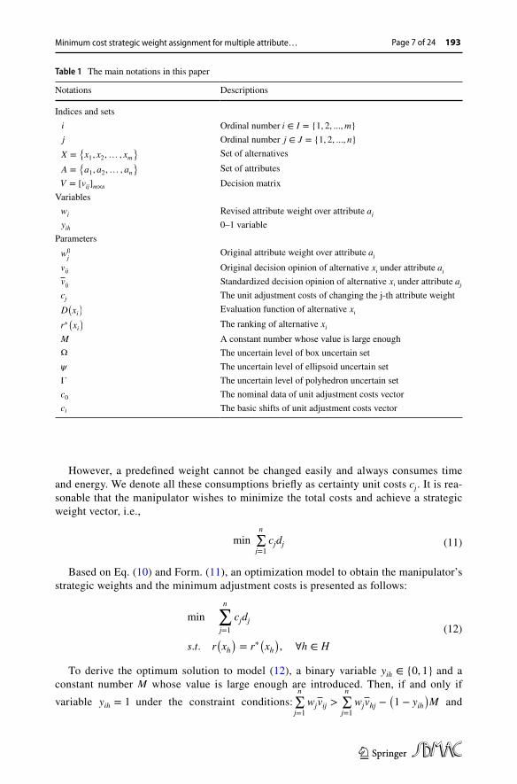
The main notations in this paper are presented in Table 1.

3 Basic minimum cost strategic weight assignment model

In MADM problems, the attribute weights usually influence the rankings of alternatives heavily. Based on this, some DMs may set the attribute weights intentionally to achieve the desired rankings of them. However, the weight cannot be modified arbitrarily and a cost always be required. In this part, a mixed 0–1 linear programming model is constructed for deriving a strategic ranking with minimum adjustment costs under WA operator.

Apparently, the weight vector’s change will lead to the change of r(xh) . Without loss of generality, we assume that the manipulator wants to assign the alternative xh in set {xh∈H|H ∈ {1, 2,… ,m}

} to the predefined ranking. Moreover, we define the ranking of

the assigned alternative xh is {r∗(xh∈H)|H ∈ {1, 2,… ,m}

} . That is, r(xh) = r∗(xh) will

be hold after strategically setting attribute weights. Assuming that the original attribute weight vector is W0 =

(w01,w0

2,… ,w0

n

)T and the revised one is W =(w1,w2,… ,wn

)T , the distance between the original and the revised j - th attribute weight can be measured by

(6)min cTx

s.t. Ax ≤ b

(A, b) ∈ U

(7)U =

{[ai;bi

]=[a0i;b0

i

]+

L∑l=1

�l

[ali;bl

i

]∶ � ∈ Z

}

(8)aTix ≤ bi ∀

��ai;bi

�=�a0i;b0

i

�+

L∑l=1

�l

�ali;bl

i

�∶ � ∈ Z

�

(9)a0ix +max

�∈Z

[L∑l=1

�l

[alix − bl

i

]]≤ b0

i

(10)dj =|||w

0j− wj

|||


123

However, a predefined weight cannot be changed easily and always consumes time and energy. We denote all these consumptions briefly as certainty unit costs cj . It is rea-sonable that the manipulator wishes to minimize the total costs and achieve a strategic weight vector, i.e.,

Based on Eq. (10) and Form. (11), an optimization model to obtain the manipulator’s strategic weights and the minimum adjustment costs is presented as follows:

To derive the optimum solution to model (12), a binary variable yih ∈ {0, 1} and a constant number M whose value is large enough are introduced. Then, if and only if variable yih = 1 under the constraint conditions:

n∑j=1

wjvij >n∑j=1

wjvhj −�1 − yih

�M and

(11)minn∑j=1

cjdj

(12)min

n∑j=1

cjdj

s.t. r(xh)= r∗

(xh), ∀h ∈ H

Table 1 The main notations in this paper

Notations Descriptions

Indices and sets i Ordinal number i ∈ I = {1, 2, ...,m}

j Ordinal number j ∈ J = {1, 2, ..., n}

X ={x1, x2,… , xm

}Set of alternatives

A ={a1, a2,… , an

}Set of attributes

V = [vij]m×n Decision matrixVariables wj Revised attribute weight over attribute aj yih 0–1 variable

Parameters w0

jOriginal attribute weight over attribute aj

vij Original decision opinion of alternative xi under attribute aj vij Standardized decision opinion of alternative xi under attribute aj cj The unit adjustment costs of changing the j-th attribute weight D(xi)

Evaluation function of alternative xi r∗

(xi)

The ranking of alternative xi M A constant number whose value is large enough Ω The uncertain level of box uncertain set � The uncertain level of ellipsoid uncertain set Γ The uncertain level of polyhedron uncertain set c0 The nominal data of unit adjustment costs vector cl The basic shifts of unit adjustment costs vector


123

n∑j=1

wjvij ≤n∑j=1

wjvhj + yihM , the evaluation value of xi is larger than xh . Else, yih = 0 and

we derive D(xi) ≤ D(xh) in that case. Then, the ranking of xh can be represented by r(xh) =

m∑i=1,i≠h

yih + 1 and must equal to a predefined ranking r∗(xh) . By requiring i ≠ h ,

the effect from the value of yhh can be eliminated. We denote the cost vector as c =

(c1, c2,… , cn

)T and distance vector as d =(d1, d2,… , dn

)T . Therefore, we transform model (12) into the mixed 0–1 programming model (13).

Proposition 1 Let gj = w0j− wj and cTd ≤ B , model (13) can be equivalently transformed

into the form of mixed 0–1 linear programming model as follows:

(13)

min cTd

s.t.

n∑j=1

wjvij >

n∑j=1

wjvhj −(1 − yih

)M, ∀i ∈ I

n∑j=1

wjvij ≤

n∑j=1

wjvhj + yihM, ∀i ∈ I,

yih = 0 or 1, ∀i ∈ I,∀h ∈ H

m∑i=1,i≠h

yih + 1 = r∗(xh), ∀h ∈ H

n∑j=1

wj = 1

0 ≤ wj ≤ 1, ∀j ∈ J

(14)

min B

s.t.

n∑j=1

wjvij >n∑j=1

wjvhj − (1 − yih)M, ∀i ∈ I

n∑j=1

wjvij ≤n∑j=1

wjvhj + yihM, ∀i ∈ I

gj = w0

j− wj, ∀j ∈ J

gj ≤ dj, ∀j ∈ J

−gj ≤ dj, ∀j ∈ J

cTd ≤ B

yih = 0 or 1, ∀i ∈ I,∀h ∈ H

m∑i=1,i≠h

yih + 1 = r∗(xh), ∀h ∈ H

n∑j=1

wj = 1

0 < wj < 1, ∀j ∈ J


123

Proof For dj =|||w0

j− wj

||| equals to dj = max{w0j− wj,−

(w0j− wj

)} , dj ≥ w0

j− wj and

dj ≥ −

(w0j− wj

) can be obtained. Let gj = w0

j− wj , the inequality constraints can be trans-

formed to dj ≥ gj and dj ≥ −gj . This completes the proof of Proposition 1.

Apparently, if the optimal solution to model (14) exists, it is possible for a manipulator to obtain the strategic ranking of an alternative. Otherwise, a strategic weight vector can-not be derived and the preferred ranking cannot be achieved. The decision variables in this model are W =

(w1,w2,… ,wn

)T and yih(h ∈ G).

4 Minimum cost strategic weight assignment model with robust optimization method

In practical cases, the costs cannot be provided in certainty form for the urgency of time or inadequacy of information. Therefore, we define the unit adjustment costs in the uncertain sets. Assume that cost c is an uncertain parameter with the data varying in the given uncer-tainty set

where c0 is nominal data, cl(l ∈ L) is basic shift, G = {1, 2,… , L}.� is a perturbation vector varying on a given perturbation set Z . The random perturbations can affect the uncertain data entries of a particular inequality constraint. c is the “true” value of an uncertain data input which is obtained from the nominal value c0 of the input and the random perturbation part (Ben-Tal and Nemirovski 2000). Then, the robust counterpart of the cost constraint of model (13) can be denoted as

Considering the worst case, it is equivalent to the following formulation.

Then, we discuss the situations when vector � is defined in three different uncertain sets.

4.1 MASWA model with box uncertain set

Consider the case of interval uncertainty, where � is defined in a box set. Box set is most robust as it contains the full range of realizations for each component of � and guaran-tees that the constraint is never violated. However, it is not very possible that all uncertain parameters can take their worst case values. Hence, the smaller uncertainty sets should be developed to enable the constraint to be “nearly never” violated (Gorissen et al. 2015).

(15)U =

{c = c0 +

L∑l=1

�lcl ∶ � ∈ Z

}

(16)cTd ≤ B,∀

(c = c0 +

L∑l=1

�lcl ∶ � ∈ Z

)

(17)cT0d +max

�∈Z

L∑l=1

�lcTld ≤ B


123

Proposition 2 If Z is a box set which is defined as ZBox =�� ∈ RL ∶ ‖�‖∞ ≤ �

�, where �

is an uncertain level parameter, the robust optimization form of model (13) can be repre-sented as

Proof According to the form of box set, the inequality (17) can be rewritten as

Then,

It is equivalent to the following worst case reformulation.

The maximum in the left side of the inequality is clearly �L∑l=1

��cTl d�� , and we achieve

the representation of cTd ≤ B by the following explicit convex constraint.

Then, adopt a representation by a system of linear inequalities

(18)

min cT0d + 𝜓

L∑l=1

ul

s.t.

n∑j=1

wjvij >n∑j=1


n∑j=1

wjvij ≤n∑j=1


gj = w0

j− wj, ∀j ∈ J


−gj ≤ dj, ∀j ∈ J

−ul ≤ cTld ≤ ul, ∀l ∈ G

yih = 0 or 1, ∀i ∈ I,∀h ∈ H

m∑i=1,i≠h

yih + 1 = r∗(xh), ∀h ∈ H

n∑j=1

wj = 1

0 < wj < 1, ∀j ∈ J

(19)cT0d +

L�l=1

�lcTld ≤ B,∀

�� ∈ RL ∶ ‖�‖∞ ≤ �

�

(20)L�l=1

�lcTld ≤ B − cT

0d,∀

�� ∈ RL ∶ ‖�‖∞ ≤ �

�

(21)max‖�‖∞≤�

L�l=1


0d

(22)cT0d + �

L∑l=1

|||cTld||| ≤ B


123

Hence, Proposition 2 is proved. And model (14) is transformed to a computationally tractable box-MASWA.

4.2 MASWA model with ellipsoid uncertain set

In this part, we will consider the case where Z is an ellipsoid set. It can be normalized by assuming that uncertain set Z is merely the ball of radius Ω centered at the origin. When the uncertainty set for a linear constraint is ellipsoid, the robust counterpart turns out to be a conic quadratic problem (Ben-Tal and Nemirovski 1999).

Proposition 3 If Z is an ellipsoid set which is defined as ZEllipsoid =�� ∈ RL ∶ ‖�‖2 ≤ Ω

�, where Ω is an uncertain level parameter, the robust optimization form of model (14) can be represented as

Proof According to the form of ellipsoid set, the inequality (17) can be rewritten as

Then,

(23)

⎧⎪⎨⎪⎩

−ul ≤ cTld ≤ ul,∀l ∈ G

cT0d + �

L�l=1

��cTld�� ≤ B

(24)

min cT0d + Ω

�L∑l=1

u2l

s.t.

n∑j=1

wjvij >n∑j=1


n∑j=1

wjvij ≤n∑j=1


gj = w0

j− wj, ∀j ∈ J


−gj ≤ dj, ∀j ∈ J


yih = 0 or 1, ∀i ∈ I,∀h ∈ H

m∑i=1,i≠h

yih + 1 = r∗(xh), ∀h ∈ H

n∑j=1

wj = 1

0 < wj < 1, ∀j ∈ J

(25)cT0d +

L�l=1

�lcTld ≤ B,∀

�� ∈ RL ∶ ‖�‖2 ≤ Ω

�


123

It is equivalent to the following worst case reformulation.

Replace original constraint cTd ≤ B with an explicit convex constraint representation as follows:

Then, adopt a representation by a system of linear inequalities

Hence, Proposition 3 is also proved, and certainty MASWA model (14) is transformed to a computationally tractable ellipsoid-MASWA.

4.3 MASWA model with polyhedron uncertain set

In this part, we will consider the case where Z is the intersection of ‖⋅‖∞ and ‖⋅‖1 . First, consider a rather general case when the perturbation set Z in (16) is defined with a conic representation

where K is a closed convex pointed cone in RN and has a nonempty interior,P,Q are given matrices and p is a given vector. In the case when K is not a polyhedral cone, assume that the following representation is strictly feasible.

Definition 1 (Ben-Tal et al. 2009) Let the perturbation set Z be defined as (30). Consider the case of non-polyhedral K and let also (31) take place. Then the semi-infinite constraint (16) can be represented by a series of conic inequalities with variables d ∈ Rn, y ∈ RN:

(26)L�l=1


0d,∀

�� ∈ RL ∶ ‖�‖2 ≤ Ω

�

(27)max‖�‖2≤Ω

L�l=1


0d

(28)cT0d + Ω

√√√√ L∑l=1

(cTld)2

≤ B

(29)

⎧⎪⎪⎨⎪⎪⎩

−ul ≤ cTld ≤ ul,∀l ∈ G

cT0d + Ω

�� L�l=1

u2l≤ B

(30)Z ={� ∈ RL ∶ ∃� ∈ RK ∶ P� + Q� + p ∈ K

}

(31)∃

(�,�

)∶ P� + Q� + p ∈ int K.


123

where K∗ ={y ∶ yTz ≥ 0∀z ∈ K

} is the cone dual to K.

Proof We have d is feasible for (16)

The result shows that d is feasible for (16) if and only if the optimal value in the conic program

is ≤ −(cT0d − B

) . First, assume that (31) takes place. Then (CP) is strictly feasible, and

applying the Conic Duality Theorem, the optimal value in (CP) is ≤ −(cT0d − B

) if and

only if the optimal value in the conic dual to the (CP) problem

is achieved and is ≤ −(cT0d − B

) . Now assume that K is a polyhedral cone. According

to the LO Duality Theorem, the same conclusion can be yielded: the optimal value in (CP) is ≤ −

(cT0d − B

) if and only if there is the optimal value in (CD) and the value is

≤ −(cT0d − B

) . In other words, under the premise of the Definition, d is feasible for (16) if

and only if (CD) has a feasible solution y with PTy ≤ −(cT0d − B

) . Hence, Definition 1 is

proved.

Definition 2 (Ben-Tal et al. 2009) When the cone K participating in (30) is the direct prod-uct of simpler cones K1, …Ks, representation (30) can take the form

In this case, (32) becomes the system of conic constraints in variables d, y1,… , ys as follows:

(32)

⎧⎪⎪⎨⎪⎪⎩

pTy + cT0d ≤ B

QTy = 0

(pTy)l + cTld = 0,∀l ∈ G

y ∈ K∗

⇔ sup�∈Z

{cT0d − B +

L∑l=1

�lcTld

}≤ 0

⇔ sup�∈Z

L∑l=1

�lcTld ≤ −

(cT0d − B

)

⇔ max�,v

{L∑l=1

�lcTld ∶ P� + Qv + p ∈ K

}≤ −

(cT0d − B

)

max�,v

{L∑l=1

�lcTld ∶ P� + Qv + p ∈ K

}(CP)

miny

{pTy ∶ QTy = 0,PTy = −

(cT0d − B

), y ∈ K∗

}, (CD)

(33)Z ={� ∶ ∃�1,… ,�s ∶ Ps� + Qs�

s + ps ∈ Ks, s = 1,… , S}


123

where Ks∗ is the cone dual to Ks.

Proposition 4 If Z is a polyhedron set or what we called budgeted uncertainty set which is defined as Zpolyhedron =

�� ∈ RL ∶ ‖�‖∞ ≤ 1, ‖�‖1 ≤ Γ

�, where Γ is an uncertain level

parameter, the robust optimization form of model (14) can be represented as

Proof According to Zpolyhedron =�� ∈ RL ∶ ‖�‖∞ ≤ 1, ‖�‖1 ≤ Γ

� , the cone representation

of representation (33) becomes Z ={� ∈ RL ∶ P1� + p1 ∈ K1,P2� + p2 ∈ K2

} , where

• P1� ≡ [�;0],p1 = [0L×1;1],K1 =�[z;t] ∈ RL × R ∶ t ≥ ‖z‖∞

� , whence

K1∗=�[z;t] ∈ RL × R ∶ t ≥ ‖z‖1

�;

• P2� ≡ [�;0],p2 = [0L×1;Γ] and K2 = K1∗=�[z;t] ∈ RL × R ∶ t ≥ ‖z‖1

� , whence

K2∗= K1.

Setting y1 = [z;�1],y2 = [�;�2] with one-dimensional � and L-dimensional z,� , sys-tem (34) becomes the following system of constraints.

(34)

⎧⎪⎪⎪⎪⎨⎪⎪⎪⎪⎩

S�s=1

pTsys + cT

0d ≤ B

QTsys = 0, s = 1,… , S

S�s=1

�PTsys�l+ cT

ld = 0, ∀l ∈ G

ys ∈ Ks∗, s = 1,… , S

(35)

min cT0d +

L∑l=1

��zl�� + Γmaxl

��𝜔l��

s.t. zl + 𝜔l = −cTld, ∀l ∈G

n∑j=1

wjvij >n∑j=1


n∑j=1

wjvij ≤n∑j=1


gj = w0

j− wj, ∀j ∈ J


−gj ≤ dj, ∀j ∈ J


yih = 0 or 1, ∀i ∈ I,∀h ∈ H

m∑i=1,i≠h

yih + 1 = r∗(xh), ∀h ∈ H

n∑j=1

wj = 1

0 < wj < 1, ∀j ∈ J


123

�1, �2, z,�, d are variables among them. We can eliminate the � variables, obtain a repre-

sentation of cTd ≤ B,∀

�c = c0 +

L∑l=1

�lcl ∶ � ∈ Z

� and

Zpolyhedron =�� ∈ RL ∶ ‖�‖∞ ≤ 1, ‖�‖1 ≤ Γ

� by the following system of constraints in var-

iables z,�, d:

Therefore, Proposition 4 is also proved in detail. And we transform model (14) to poly-hedron-MASWA. To the convenience for later numerical analysis, we denote model (14) as P1, model (18) as P2, model (24) as P3 and model (35) as P4 in this paper.

5 Numerical example and comparative analysis

In this section, an example about the assessment of the anti-epidemic performance of the 14 provinces and cities is explored to demonstrate the validity of the proposed MASWA models, and how the models work. A comparative performance analysis between the cer-tainty strategic weight assignment model and the three robust strategic weight assignment models is provided to show the effects of uncertainty. Moreover, further analysis for detect-ing the influence of different uncertain levels is also included. The MATLAB 2020a is used to write the necessary programs and calculate the models, couples with the YALMIP toolbox.

5.1 Background description

The newly identified infectious coronavirus COVID-19 was first reported in Wuhan of China since December 2019 and has been discovered in many other countries around the globe (Chen et al. 2020). It can cause a sudden respiratory infection, which is often mild among children and healthy adults, but is much more fatal to old people and those with healthy problems. The spread of the epidemic has brought huge losses to the economy and seriously affected people’s normal life. To resist the spread of COVID-19 and reduce the influence on the economy, almost every region in China reacts to the virus quickly by screening for COVID-19 in large numbers such as maintaining social distance policies and emphasizing wearing a mask. Considering the different epidemic situation of different provinces and cities, we can use some indicators to evaluate the performance of them. The assessment of anti-epidemic performance is usually connected to the work efficiency and emergency management capacity of local government. To demonstrate the validity of our

(36)

⎧⎪⎪⎨⎪⎪⎩

�1 + Γ�2 + cT0d ≤ B

(z + �)l = −cTld,∀l ∈ G

‖z‖1 ≤ �1

‖�‖∞ ≤ �2

(37)

⎧⎪⎨⎪⎩

L�l=1

��zl�� + Γmaxl

��l�� + cT

0d ≤ B

zl + �l = −cTld,∀l ∈ G


123

models, we select some epidemic data from January to May of 2020, which is also a period of concentrated outbreak.

Different weight attributes may lead to completely different ranking results. By studying how the strategic weight assignment works, it is meaningful for future research on avoiding the manipulation of alternative ranking. It is also very important for developing more rea-sonable ranking methods. Through an evaluation process, we assess the 14 provinces and cities

{x1, x2,… , x14

} from the five aspects

{a1, a2, a3, a4, a5

} . The description of the five

attributes is presented in the following Table 2.

5.2 Numerical analysis

As we can see, the relevant actual data is presented in Table 2. Through the normalization process, the normalized decision matrix V = [vij]14×5 is obtained (see Table 3). Let W =

(w01,w0

2,w0

3,w0

4,w0

5

)T be the initial attribute weight vector, where w01= w0

2= w0

3= w0

4= w0

5= 0.2 . Then, assume that the cost vector for changing the corre-

sponding attribute is c = (6, 9, 8, 7, 5)T . Considering the uncertainty of costs,

c̃ = c0 +L∑l=1

𝜉lcl , where c0 = c = (6, 9, 8, 7, 5)T,L = 3.cl(l = 1, 2, 3) is randomly generated as

c1 = (−1, 0.6,−0.5, 0.7,−0.4),c2 = (0.5,−0.7, 0.3,−0.9, 0.4) and

Table 2 Five attributes in evaluating the 14 provinces and cities

We can find that a2 is a benefit attribute, and find that a1, a3, a4 and a5 are cost attributes.

Attributes Descriptions

a1 Number of confirmed COVID-19 casesa2 Number of curea3 Number of deathsa4 Number of close contactsa5 Number of medical observers

Table 3 The data of the anti-epidemic performances of the 14 provinces and cities

Province/city a1 a2 a3 a4 a5

x1 1273 1251 22 40265 2096x2 1018 1014 4 27415 1362x3 763 756 7 21830 1314x4 1218 1217 1 48710 2689x5 990 984 6 29323 572x6 146 144 2 2577 119x7 91 89 2 4337 209x8 136 133 3 3524 275x9 318 312 6 11223 640x10 134 134 0 5104 266x11 631 631 0 13642 860x12 18 18 0 437 47x13 168 162 6 6787 328x14 576 570 6 25111 1264


123

c3 = (−0.6, 0.4, 0.5,−0.7, 0.6) . Moreover, we set the uncertain levels � = 1 in model P2, Ω = 1 in model P3 and Γ = 1 in model P4.

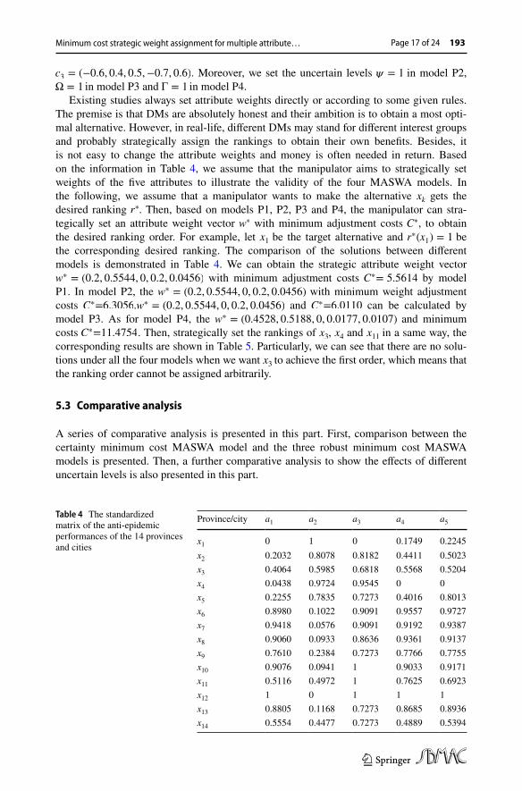
Existing studies always set attribute weights directly or according to some given rules. The premise is that DMs are absolutely honest and their ambition is to obtain a most opti-mal alternative. However, in real-life, different DMs may stand for different interest groups and probably strategically assign the rankings to obtain their own benefits. Besides, it is not easy to change the attribute weights and money is often needed in return. Based on the information in Table 4, we assume that the manipulator aims to strategically set weights of the five attributes to illustrate the validity of the four MASWA models. In the following, we assume that a manipulator wants to make the alternative xk gets the desired ranking r∗ . Then, based on models P1, P2, P3 and P4, the manipulator can stra-tegically set an attribute weight vector w∗ with minimum adjustment costs C∗ , to obtain the desired ranking order. For example, let x1 be the target alternative and r∗(x1) = 1 be the corresponding desired ranking. The comparison of the solutions between different models is demonstrated in Table 4. We can obtain the strategic attribute weight vector w∗ = (0.2, 0.5544, 0, 0.2, 0.0456) with minimum adjustment costs C∗= 5.5614 by model P1. In model P2, the w∗ = (0.2, 0.5544, 0, 0.2, 0.0456) with minimum weight adjustment costs C∗=6.3056.w∗ = (0.2, 0.5544, 0, 0.2, 0.0456) and C∗=6.0110 can be calculated by model P3. As for model P4, the w∗ = (0.4528, 0.5188, 0, 0.0177, 0.0107) and minimum costs C∗=11.4754 . Then, strategically set the rankings of x3 , x4 and x11 in a same way, the corresponding results are shown in Table 5. Particularly, we can see that there are no solu-tions under all the four models when we want x3 to achieve the first order, which means that the ranking order cannot be assigned arbitrarily.

5.3 Comparative analysis

A series of comparative analysis is presented in this part. First, comparison between the certainty minimum cost MASWA model and the three robust minimum cost MASWA models is presented. Then, a further comparative analysis to show the effects of different uncertain levels is also presented in this part.

Table 4 The standardized matrix of the anti-epidemic performances of the 14 provinces and cities

Province/city a1 a2 a3 a4 a5

x1 0 1 0 0.1749 0.2245x2 0.2032 0.8078 0.8182 0.4411 0.5023x3 0.4064 0.5985 0.6818 0.5568 0.5204x4 0.0438 0.9724 0.9545 0 0x5 0.2255 0.7835 0.7273 0.4016 0.8013x6 0.8980 0.1022 0.9091 0.9557 0.9727x7 0.9418 0.0576 0.9091 0.9192 0.9387x8 0.9060 0.0933 0.8636 0.9361 0.9137x9 0.7610 0.2384 0.7273 0.7766 0.7755x10 0.9076 0.0941 1 0.9033 0.9171x11 0.5116 0.4972 1 0.7625 0.6923x12 1 0 1 1 1x13 0.8805 0.1168 0.7273 0.8685 0.8936x14 0.5554 0.4477 0.7273 0.4889 0.5394


123

5.3.1 Comparison on the performances of different MASWA models

This section presents a fair comparative study between MASWA model based on deter-ministic unit adjustment costs, and the three robust MASWA models based on uncertain unit adjustment costs. To save space, we only select alternatives x2 and x10 to illustrate the four models.

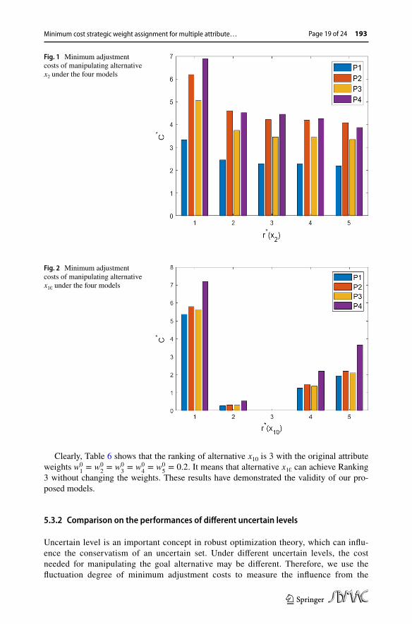
From Figs. 1 and 2, we can see the minimum adjustment costs on manipulating x2 and x10 from Ranking 1 to Ranking 5 by the proposed four models. For the three robust cases, in comparison with the deterministic model P1, all the three robust minimum adjustment costs are higher than that under certainty situation. It means that it often cost more when cost varying on uncertain sets. Therefore, in real-life decision-making problems, information should be collected extensively to reduce the uncertainty of the environment, so as to reduce the decision-making costs. On the contrary, the uncertainty of weight modification costs can also be increased to increase the difficulty of adjust-ing attribute weights and suppress the strategy weight assignment behavior. In Fig. 2, we can find that all the minimum adjustment costs obtained by the four models equal to zero when we assign x10 to Ranking 3.

To explore the rationality of the results, we calculate the evolution values of the 14 alternatives by Eq. (3), with data in Table 4 and w0

1= w0

2= w0

3= w0

4= w0

5= 0.2 . The

calculation results are shown in Table 6.

Table 5 The results of manipulating particular alternatives under different MASWA models

Target alternative r∗ Model C

∗w∗

x1 1 P1

P2

P3

P4

5.5614

6.3056

6.0110

11.4754

(0.2, 0.5544, 0, 0.2, 0.0456)

(0.2, 0.5544, 0, 0.2, 0.0456)

(0.2, 0.5544, 0, 0.2, 0.0456)

(0.4528, 0.5188, 0, 0.0177, 0.0107)

x3 3 P1

P2

P3

P4

5.7394

6.2936

6.0743

8.9923

(0.2, 0.4639, 0.0126, 0.3235, 0)

(0.2, 0.4639, 0.0126, 0.3235, 0)

(0.2, 0.4639, 0.0126, 0.3235, 0)

(0.0794, 0.4498, 0.021, 0.4498, 0)

x4 1 P1

P2

P3

P4

3.5706

4.0918

3.8855

5.6747

(0.2, 0.4482, 0.2, 0.1518, 0)

(0.2, 0.4482, 0.2, 0.1518, 0)

(0.2, 0.4482, 0.2, 0.1518, 0)

(0.2, 0.3576, 0.3576, 0.0424, 0.0424)

x11 2 P1

P2

P3

P4

1.5745

1.7949

1.7077

2.7741

(0.095, 0.305, 0.2, 0.2, 0.2)

(0.095, 0.305, 0.2, 0.2, 0.2)

(0.095, 0.305, 0.2, 0.2, 0.2)

(0.1229, 0.2771, 0.2771, 0.2, 0.1229)

x3 1 P1

P2

P3

P4

No solution No solution


123

Clearly, Table 6 shows that the ranking of alternative x10 is 3 with the original attribute weights w0

1= w0

2= w0

3= w0

4= w0

5= 0.2 . It means that alternative x10 can achieve Ranking

3 without changing the weights. These results have demonstrated the validity of our pro-posed models.

5.3.2 Comparison on the performances of different uncertain levels

Uncertain level is an important concept in robust optimization theory, which can influ-ence the conservatism of an uncertain set. Under different uncertain levels, the cost needed for manipulating the goal alternative may be different. Therefore, we use the fluctuation degree of minimum adjustment costs to measure the influence from the

Fig. 1 Minimum adjustment costs of manipulating alternative x2 under the four models

Fig. 2 Minimum adjustment costs of manipulating alternative x10 under the four models


123

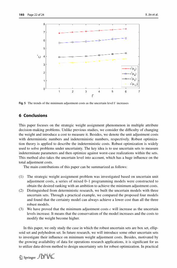
changing of uncertain levels. For example, we select alternatives x2,x4,x5 and x11 , and then set them to Ranking 1, respectively. Change the uncertain levels � , Ω and Γ in the three robust models from 1 to 6. Then, the results of the minimum adjustment costs are shown in Tables 7, 8 and 9. To the facility of observation, we plot the results in Figs. 3, 4 and 5.

From the three figures, we can see that the minimum adjustment costs under all the three robust models of the four alternatives increase as uncertain levels increase. It means that the conservatism of a model increases with the increasing of uncertain lev-els. It also means that it will be more difficult to assign the ranking of alternatives.

Table 6 The evolution values of the 14 alternatives with original attribute weights

xi D(xi) r(xi)

x1 0.2799 14x2 0.5545 10x3 0.5528 11x4 0.3941 13x5 0.5878 9x6 0.7675 2x7 0.7533 4x8 0.7425 5x9 0.6558 8x10 0.7644 3x11 0.6855 7x12 0.800 1x13 0.6973 6x14 0.5517 12

Table 7 The comparison of minimum adjustment costs under different uncertain levels �

xi r∗

C∗

�= 1 �= 2 �= 3 �= 4 �= 5 �= 6

x2 1 3.8054 4.2828 4.7602 5.2377 5.7151 6.1925x4 1 4.0918 4.6129 5.1341 5.6552 6.1749 6.5574x5 1 2.8520 3.1009 3.3498 3.5987 3.8477 4.0966x11 1 1.9862 2.2301 2.4741 2.7180 2.9619 3.2058

Table 8 The comparison of minimum adjustment costs under different uncertain levels Ω

xi r∗

C∗

Ω = 1 Ω = 2 Ω = 3 Ω = 4 Ω = 5 Ω = 6

x2 1 3.6165 3.9049 4.1934 4.4818 4.7703 5.0588x4 1 3.8855 4.2004 4.5153 4.8302 5.1451 5.4600x5 1 2.7534 2.9038 3.0542 3.2047 3.3551 3.5055x11 1 1.8897 2.0371 2.1844 2.3318 2.4792 2.6266


123

Table 9 The comparison of minimum adjustment costs under different uncertain levels Γ

xi r∗

C∗

Γ = 1 Γ = 2 Γ = 3 Γ = 4 Γ = 5 Γ = 6

x2 1 6.8822 6.9969 7.0925 7.1952 7.3025 7.4132x4 1 5.6747 5.7693 5.8481 5.9713 6.1479 6.2613x5 1 3.9014 3.9664 4.0206 4.1462 4.2982 4.4014x11 1 3.1866 3.2397 3.2840 3.4610 3.6052 3.7114

Fig. 3 The trends of the minimum adjustment costs as the uncertain level � increases

Fig. 4 The trends of the minimum adjustment costs as the uncertain level Ω increases


123

6 Conclusions

This paper focuses on the strategic weight assignment phenomenon in multiple attribute decision-making problems. Unlike previous studies, we consider the difficulty of changing the weight and introduce a cost to measure it. Besides, we denote the unit adjustment costs with deterministic numbers and indeterministic numbers, respectively. Robust optimiza-tion theory is applied to describe the indeterministic costs. Robust optimization is widely used to solve problems under uncertainty. The key idea is to use uncertain sets to measure indeterminate parameters and then optimize against worst-case realizations within the sets. This method also takes the uncertain level into account, which has a huge influence on the total adjustment costs.

The main contributions of this paper can be summarized as follows:

(1) The strategic weight assignment problem was investigated based on uncertain unit adjustment costs, a series of mixed 0–1 programming models were constructed to obtain the desired ranking with an ambition to achieve the minimum adjustment costs.

(2) Distinguished from deterministic research, we built the uncertain models with three uncertain sets. Through a practical example, we compared the proposed four models and found that the certainty model can always achieve a lower cost than all the three robust models.

(3) We have proved that the minimum adjustment costs c will increase as the uncertain levels increase. It means that the conservatism of the model increases and the costs to modify the weight become higher.

In this paper, we only study the case in which the robust uncertain sets are box set, ellip-soid set and polyhedron set. In future research, we will introduce some other uncertain sets to investigate their influence on minimum weight adjustment costs. Besides, motivated by the growing availability of data for operations research applications, it is significant for us to utilize data-driven method to design uncertainty sets for robust optimization. In practical

Fig. 5 The trends of the minimum adjustment costs as the uncertain level Γ increases


123

MADM problems, there are often many DMs participating in the discussion. Therefore, it is also meaningfully for us to study strategic weight assignment in large-scale group decision-making.

Acknowledgements We thank for the consideration of the editor and the insightful comments of reviewers.

Funding This work is supported by the Science and Technology Commission of Shanghai Municipality (No. 2020BGL010).

References

Ben-Arieh D, Easton T (2007) Multi-criteria group consensus under linear cost opinion elasticity. Decis Support Syst 43:713–721

Ben-Arieh D, Easton T, Evans B (2008) Minimum cost consensus with quadratic cost functions. IEEE Trans Syst Man Cybern Syst Hum 39(1):210–217

Ben-Tal A, Nemirovski A (1999) Robust solutions of uncertain linear programs. Oper Res Lett 25:1–13Ben-Tal A, Nemirovski A (2000) Robust solutions of linear programming problems contaminated with

uncertain data. Math Progr Ser A 88:411–424Ben-Tal A, Nemirovski A (2009) Robust convex optimization. Math Oper Res 23(4):769–805Ben-Tal A, Ghaoui L, Nemirovski A (2009) Robust optimization. Princeton University PressBertsimas D, Sim M (2012) The price of robustness. Oper Res 52(1):35–53Capuano N, Chiclana F, Fujita H, Herrera-viedma E (2018) Fuzzy group decision making with incomplete

information guided by social influence. IEEE Trans Fuzzy Syst 26(3):1704–1718Chen N, Zhou M, Dong X, Qu J, Gong F, Han Y, Qiu Y, Wang J, Liu Y, Wei Y, Xia J, Yu T, Zhang X,

Zhang L (2020) Epidemiological and clinical characteristics of 99 cases of 2019 novel coronavirus pneumonia in Wuhan, China: a descriptive study. Lancet 395:507–513

Cheng D, Zhou Z, Cheng F, Zhou Y, Xie Y (2018) Modeling the minimum cost consensus problem in an asymmetric costs context. Eur J Oper Res 270:1122–1137

Dong YC, Zhang HJ, Herrera-Viedma E (2016) Consensus reaching model in the complex and dynamic MAGDM problem. Knowl Based Syst 106:206–219

Dong YC, Liu YT, Liang HM, Chiclana F, Herrera-Viedma E (2018) Strategic weight assignment in multi-ple attribute decision making. Omega 75:154–164

Geldermann J, Bertsch V, Treitz M, French S, Papamichail KN, Hämäläinen RP (2009) Multi-criteria deci-sion support and evaluation of strategies for nuclear remediation management. Omega 37:238–251

Gong ZW, Zhang HH, Forrest J, Li LS, Xu XX (2015) Two consensus models based on the minimum cost and maximum return regarding either all individuals or one individual. Eur J Oper Res 240:183–192

Gorissen BL, Yanikoğlu I, Hertog DD (2015) A practical guide to robust optimization. Omega 53:124–137Gou XJ, Xu ZS, Liao HC (2019) Hesitant fuzzy linguistic possibility degree-based linear assignment

method for multiple criteria decision-making. Int J Inf Technol Decis 18(1):35–63Gou XJ, Xu ZS, Liao HC, Herrera F (2020) Probabilistic double hierarchy linguistic term set and its use in

designing an improved VIKOR method: the application in smart healthcare. J Oper Res Soc. https:// doi. org/ 10. 1080/ 01605 682. 2020. 18067 41

Han YF, Qu SJ, Wu Z (2020) Distributionally robust chance constrained optimization model for the mini-mum cost consensus. Int J Fuzzy Syst 22(6):2041–2054

Horsky D, Rao MR (1984) Estimation of attribute weights from preference comparisons. Manag Sci 30(7):801–822

Huang RP, Qu SJ, Gong ZW, Goh M, Ji Y (2020) Data-driven two-stage distributionally robust optimization with risk aversion. Appl Soft Comput J 87:105978

Ji Y, Du JH, Han XY, Wu XQ, Huang RP, Wang SL, Liu ZM (2020) A mixed integer robust program-ming model for two-echelon inventory routing problem of perishable products. Phys Stat Mech Appl 548:124481

Labella A, Liu HB, Rodríguez RM, Martínez L (2020) A cost consensus metric for consensus reaching pro-cesses based on a comprehensive minimum cost model. Eur J Oper Res 281(2):316–331

Liu YT, Dong YC, Liang HM, Chiclana F, Herrera-Viedma E (2019) Multiple attribute strategic weight assignment with minimum cost in a group decision making context with interval attribute weights information. IEEE Trans Syst Man Cybern Syst 49:1981–1992

https://doi.org/10.1080/01605682.2020.1806741

https://doi.org/10.1080/01605682.2020.1806741


123

Lourenço JC, Morton A, Costa CAB (2012) PROBE—-a multicriteria decision support system for portfolio robustness evaluation. Decis Support Syst 54:534–550

Palomares I, Martínez L, Herrera F (2014) A consensus model to detect and manage noncooperative behav-iors in large-scale group decision making. IEEE Trans Fuzzy Syst 22(3):516–530

Pekelman D, Sen SK (1974) Mathematical programming models for the determination of attribute weights. Manag Sci 20(8):1217–1229

Qu SJ, Han YF, Wu Z, Raza H (2020) Consensus modeling with asymmetric cost based on data-driven robust optimization. Group Decis Negot. https:// doi. org/ 10. 1007/ s10726- 020- 09707-w

Qu SJ, Li YM, Ji Y (2021) The mixed integer robust maximum expert consensus models for large-scale GDM under uncertainty circumstances. Appl Soft Comput J 107:107369

Roberts R, Goodwin P (2002) Weight approximations in multi-attribute decision models. J Multi Crit Decis Anal 11(6):291–303

Saaty TL (2013) The modern science of multicriteria decision making and its practical applications: the AHP/ANP approach. Oper Res 61(5):1101–1118

Shirland LE, Jesse RR, Thompson RL, Iacovou CL (2003) Determining attribute weights using mathemati-cal programming. Omega 31(6):423–437

Tan X, Gong ZW, Chiclana F, Zhang N (2017) Consensus modeling with cost chance constraint under uncertainty opinions. Appl Soft Comput J 49:1–20

Tang M, Liao HC (2021) Multi-attribute large-scale group decision making with data mining and subgroup leaders: an application to the development of the circular economy. Technol Forescast Soc Change 167:120719

Wang XJ, Curry DJ (2012) A robust approach to the share-of-choice product design problem. Omega 40:818–826

Wei G (2015) Approaches to interval intuitionistic trapezoidal fuzzy multiple attribute decision making with incomplete weight information. Int J Fuzzy Syst 17:484–489

Wei G (2017) Picture 2-tuple linguistic bonferroni mean operators and their application to multiple attribute decision making. Int J Fuzzy Syst 19:997–1010

Wiesemann W, Kuhn D, Sim M (2014) Distributionally robust convex optimization. Oper Res 62(6):1358–1376

Xu XH, Du ZJ, Chen XH (2015) Consensus model for multi-criteria large-group emergency decision mak-ing considering non-cooperative behaviors and minority opinions. Decis Support Syst 79:150–160

Yager RR (2001) Penalizing strategic preference assignment in multi-agent decision making. IEEE Trans Fuzzy Syst 9(3):393–403

Yager RR (2002) Defending against strategic assignment in uninorm-based multi-agent decision making. Eur J Oper Res 141:217–232

Yager RR (2018) Multi-criteria decision making with interval criteria satisfactions using the golden rule representative value. IEEE Trans Fuzzy Syst 26(2):1023–1031

Yan S, Tang CH (2009) Inter-city bus scheduling under variable market share and uncertain market demands. Omega 37:178–192

Zhang GQ, Dong YC, Xu YF, Li HY (2011) Minimum-cost consensus models under aggregation operators. IEEE Trans Syst Man Cybern Syst Hum 41(6):1253–1261

Publisher’s Note Springer Nature remains neutral with regard to jurisdictional claims in published maps and institutional affiliations.

https://doi.org/10.1007/s10726-020-09707-w

minimum cost strategic weight assignment for multiple

Documents