minimizing load shedding in electricity networks by preventive · pdf file ·...
TRANSCRIPT
Minimizing load shedding in electricity networks bypreventive islanding
Waqquas Bukhsh, Andreas Grothey, Ken McKinnon,Jacek Gondzio, Paul Trodden
School of MathematicsUniversity of Edinburgh
FERC25th June 2012
Background
Project structure
◮ EPSRC funded project led by Janusz Bialek at Durham Universitywith groups at Edinburgh and Southampton.
Group Responsibilities:
◮ Durham: Electrical Engineering: System dynamics
◮ Southampton: Mathematics: Laplacian based graph partitioning
◮ Edinburgh: OR and Optimization: Steady state optimization
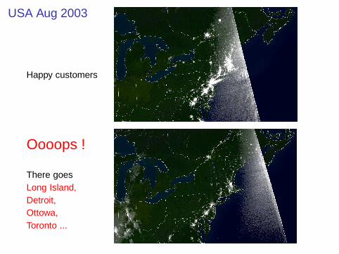
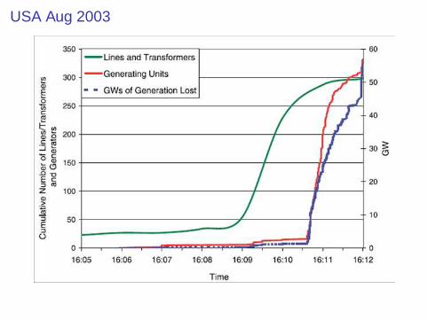
USA Aug 2003
Happy customers
Oooops !
There goesLong Island,Detroit,Ottowa,Toronto ...
USA Aug 2003
Background
Goal
◮ Develop a tool that can create a Firewall to isolate the troubledarea from the rest of the network.
◮ Leave network in a stable steady state.
◮ Could be used for off line analysis to prepare responses to faultsin different areas or, if fast enough, to react in real time.

Sectioning “uncertain” parts of network
◮ Network has “uncertain” buses/lines/generators ? ? ?
??
? ?
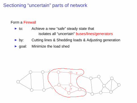
Sectioning “uncertain” parts of network
Form a Firewall
◮ to: Achieve a new “safe” steady state thatisolates all “uncertain” buses/lines/generators
◮ by: Cutting lines & Shedding loads & Adjusting generation
◮ goal: Minimize the load shed
?
??
?

Sectioning “uncertain” parts of network
◮ Section 0 – uncertain parts, Section 1 – certain parts
◮ All load in section 0 is at risk, with chance β of surviving
?
??
?
Island 1 Island 2
Section 0 Section 1Section 1
Island 3 Island 4

Sectioning with uncertainty: β = 0.5Before
~
~3
75
14
13
6
1
10
9
4
1112
2?
◮ 259 MW total load
◮ 0.0 MW load shed
◮ 129.5 expected loss
After
~
~3
75
14
13
6
1
10
9
4
1112
2?
◮ 0.0 MW shed in Section 1
◮ 35.9 MW shed in Section 0
◮ 127.8 MW at risk in Section 0
◮ 99.8 MW expected loss

Growth of section 0 in 24 bus network as β → 1
0.00 ≤ β ≤ 1.00~ ~~
~
~~ ~ ~
~ ~~
2118 22
16 19
17
12
15 14 13
9 10
1 2 7
4
11
8
2320
65
24
3?
?
?
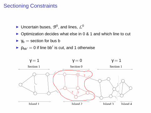
Sectioning Constraints
◮ Uncertain buses, B0, and lines, L0
◮ Optimization decides what else in 0 & 1 and which line to cut
◮ γb = section for bus b
◮ ρbb′ = 0 if line bb′ is cut, and 1 otherwise
γ = 1 γ = 0 γ = 1
?
??
?
Island 1 Island 2
Section 0 Section 1Section 1
Island 3 Island 4
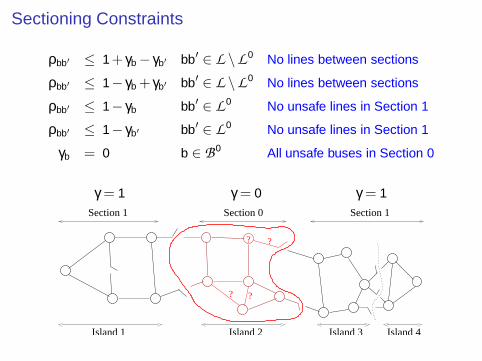
Sectioning Constraints
ρbb′ ≤ 1+ γb − γb′ bb′ ∈ L \L0 No lines between sections
ρbb′ ≤ 1− γb + γb′ bb′ ∈ L \L0 No lines between sections
ρbb′ ≤ 1− γb bb′ ∈ L0 No unsafe lines in Section 1
ρbb′ ≤ 1− γb′ bb′ ∈ L0 No unsafe lines in Section 1
γb = 0 b ∈ B0 All unsafe buses in Section 0
γ = 1 γ = 0 γ = 1
?
??
?
Island 1 Island 2
Section 0 Section 1Section 1
Island 3 Island 4
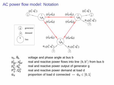
AC power flow model: Notation
3
~2
21
~1 ,( )L
12L12p q ,( )L
21L21p q
,( )L13
L13p q ,( )L
23L23p q
,( )L31
L31p q ,( )L
32L32p q
1v 1θ
3v 3θ
2v 2θ
,( )G1
G1p q ,( )G
2G2p q
,( )D2
D3p qα3
,( )D2
D2p qα2,( )D
1D1p qα1
d
b
~g
demand
generator
bus
1 2
3
vb, θb voltage and phase angle at bus bpL
bb′ ,qLbb′ real and reactive power flows into line (b,b′) from bus b
pGg ,qG
g real and reactive power output of generator gPD
d ,QDd real and reactive power demand at load d
αd proportion of load d connected — αd ∈ [0,1]
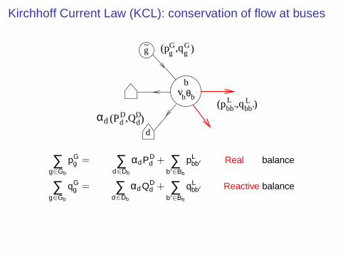
Kirchhoff Current Law (KCL): conservation of flow at buses
Gg(p G
g,q )
,qbb’L(pL )bb’
αd ),QDDd(P d
~g
bv bθb
d
∑g∈Gb
pGg = ∑
d∈Db
αdPDd + ∑
b′∈Bb
pLbb′ Real balance
∑g∈Gb
qGg = ∑
d∈Db
αd QDd + ∑
b′∈Bb
qLbb′ Reactive balance

Kirchhoff Voltage Law (KVL): flow-voltage relations on lines
G Bbb’ bb’
L(pLbb’ bb’
)^ ^,q L(pLb’b b’b
)^ ^,qb
bv bθb’
b’v b’θ
δbb′ = θb −θb′
p̂Lbb′ = Gbb′vb(vb − vb′ cosδbb′)−Bbb′vbvb′ sinδbb′
q̂Lbb′ = Bbb′vb(vb′ cosδbb′ − vb)−Gbb′vbvb′ sinδbb′ − v2
b Cbb′
◮ Because of power losses in the lines
p̂Lbb′ 6= −p̂L
b′b and q̂Lbb′ 6= −q̂L
b′b.
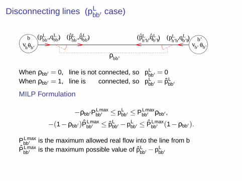
Disconnecting lines (pLbb′ case)
bv b’θ
Lbb’
(p Lbb’,q ) L
b’b(p L
b’b,q )Lb’b
(p Lb’b,q )^^L
bb’(p L
bb’,q )^^
ρbb’
vb’ b’θb b’
When ρbb′ = 0, line is not connected, so pLbb′ = 0
When ρbb′ = 1, line is connected, so pLbb′ = p̂L
bb′
MILP Formulation
−ρbb′PLmaxbb′ ≤ pL
bb′ ≤ PLmaxbb′ ρbb′ ,
−(1−ρbb′)P̂Lmaxbb′ ≤ p̂L
bb′ −pLbb′ ≤ P̂Lmax
bb′ (1−ρbb′).
PLmaxbb′ is the maximum allowed real flow into the line from b
P̂Lmaxbb′ is the maximum possible value of p̂L
bb′ −pLbb′
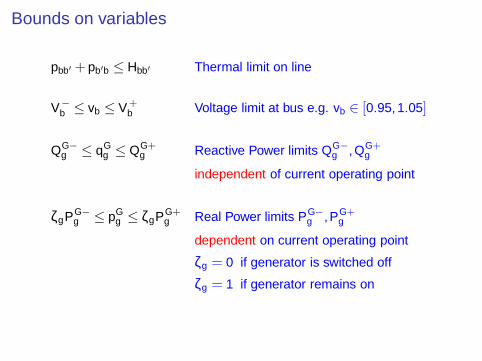
Bounds on variables
pbb′ + pb′b ≤ Hbb′ Thermal limit on line
V−b ≤ vb ≤ V +
b Voltage limit at bus e.g. vb ∈ [0.95,1.05]
QG−g ≤ qG
g ≤ QG+g Reactive Power limits QG−
g ,QG+g
independent of current operating point
ζgPG−g ≤ pG
g ≤ ζgPG+g Real Power limits PG−
g ,PG+g
dependent on current operating point
ζg = 0 if generator is switched off
ζg = 1 if generator remains on
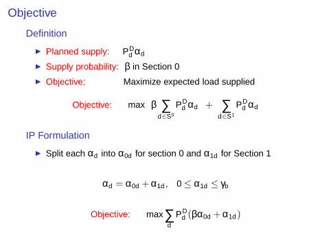
Objective
Definition
◮ Planned supply: PDd αd
◮ Supply probability: β in Section 0
◮ Objective: Maximize expected load supplied
Objective: max β ∑d∈S0
PDd αd + ∑
d∈S1
PDd αd
IP Formulation
◮ Split each αd into α0d for section 0 and α1d for Section 1
αd = α0d + α1d , 0 ≤ α1d ≤ γb
Objective: max∑d
PDd (βα0d + α1d)
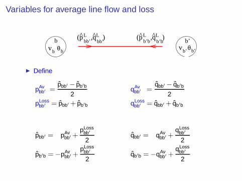
Variables for average line flow and loss
L(pLbb’ bb’
)^ ^,q L(pLb’b b’b
)^ ^,qb
bv bθb’
b’v b’θ
◮ Define
pAvbb′ =
p̂bb′ − p̂b′b
2qAv
bb′ =q̂bb′ − q̂b′b
2pLoss
bb′ = p̂bb′ + p̂b′b qLossbb′ = q̂bb′ + q̂b′b
p̂bb′ = pAvbb′ +
pLossbb′
2q̂bb′ = qAv
bb′ +qLoss
bb′
2
p̂b′b = −pAvbb′ +
pLossbb′
2q̂b′b = −qAv
bb′ +qLoss
bb′
2
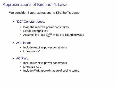
Approximations of Kirchhoff’s Laws
We consider 3 approximations to Kirchhoff’s Laws
◮ “DC” Constant Loss:
◮ Drop the reactive power constraints◮ Set all voltages to 1◮ Assume line loss pLoss
bb′ = its pre-islanding value
◮ AC Linear:◮ Include reactive power constraints◮ Linearize KVL
◮ AC PWL:◮ Include reactive power constraints◮ Linearize KVL◮ Include PWL approximation of cosine terms
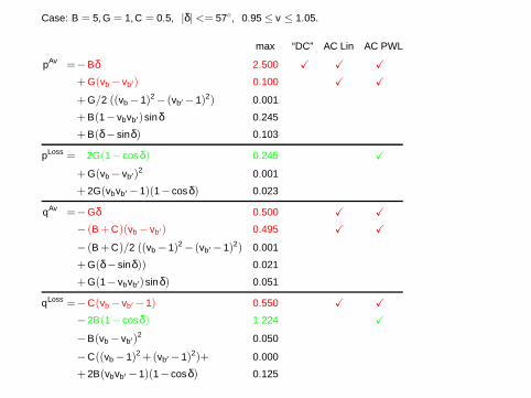
Case: B = 5,G = 1,C = 0.5, |δ| <= 57◦, 0.95 ≤ v ≤ 1.05.
max “DC” AC Lin AC PWL
pAv =−Bδ 2.500 X X X
+ G(vb − vb′) 0.100 X X
+ G/2 ((vb −1)2 − (vb′ −1)2) 0.001
+ B(1− vbvb′)sinδ 0.245
+ B(δ− sinδ) 0.103
pLoss = 2G(1− cosδ) 0.245 X
+ G(vb − vb′)2 0.001
+ 2G(vbvb′ −1)(1− cosδ) 0.023
qAv =−Gδ 0.500 X X
− (B + C)(vb − vb′) 0.495 X X
− (B + C)/2 ((vb −1)2 − (vb′ −1)2) 0.001
+ G(δ− sinδ)) 0.021
+ G(1− vbvb′)sinδ) 0.051
qLoss =−C(vb − vb′ −1) 0.550 X X
−2B(1− cosδ) 1.224 X
−B(vb − vb′)2 0.050
−C((vb −1)2 +(vb′ −1)2)+ 0.000
+ 2B(vbvb′ −1)(1− cosδ) 0.125
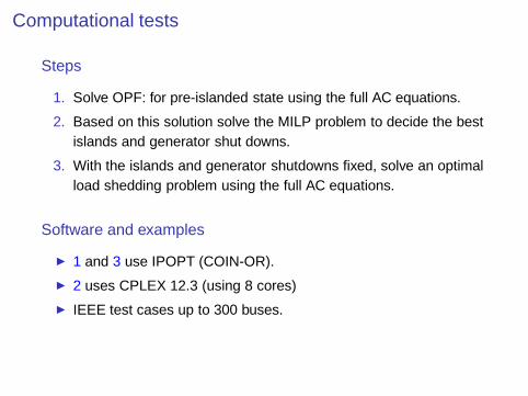
Computational tests
Steps
1. Solve OPF: for pre-islanded state using the full AC equations.
2. Based on this solution solve the MILP problem to decide the bestislands and generator shut downs.
3. With the islands and generator shutdowns fixed, solve an optimalload shedding problem using the full AC equations.
Software and examples
◮ 1 and 3 use IPOPT (COIN-OR).
◮ 2 uses CPLEX 12.3 (using 8 cores)
◮ IEEE test cases up to 300 buses.

Computational Times (DC constant loss)Min, Median and Max
nB
t com
p(s
)
feasible
5%
1%
optimal
9 14 24 30 39 57 118 30010−2
10−1
1
101
102
103
104
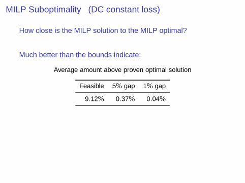
MILP Suboptimality (DC constant loss)
How close is the MILP solution to the MILP optimal?
Much better than the bounds indicate:
Average amount above proven optimal solution
Feasible 5% gap 1% gap
9.12% 0.37% 0.04%
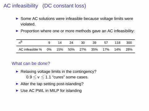
AC infeasibility (DC constant loss)
◮ Some AC solutions were infeasible because voltage limits wereviolated.
◮ Proportion where one or more methods gave an AC infeasibility:
nB 9 14 24 30 39 57 118 300
AC infeasible % 0% 15% 50% 27% 35% 17% 14% 28%
What can be done?
◮ Relaxing voltage limits in the contingency?0.9 ≤ v ≤ 1.1 “cures” some cases.
◮ Alter the tap setting post-islanding?
◮ Use AC PWL in MILP for islanding
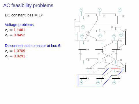
AC feasibility problems
DC constant loss MILP
Voltage problemsv2 = 1.1461v6 = 0.8452
Disconnect static reactor at bus 6:v2 = 1.0709v6 = 0.9291
~ ~~
~
~~ ~ ~
~ ~~
2118 22
16 19
17
12
15 14 13
9 10
1 2 7
4
11
8
2320
5
24
3
?6

AC feasibility problem solved
AC PWL MILP
No Voltage problemsv2 = 1.02v6 = 0.9851v10 = 0.9984
~ ~~
~
~~ ~ ~
~ ~~
2118 22
16 19
17
12
15 14 13
9 10
1 2 7
4
11
8
2320
5
24
3
?6
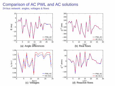
Comparison of AC PWL and AC solutions24-bus network: angles, voltages & flows
Line l
δL l(d
eg)
PWL-ACAC-OLS
0 5 10 15 20 25 30−20
−15
−10
−5
0
5
10
(a) Angle differencesLine l
pL,
frl
(MW
)
PWL-ACAC-OLS
0 5 10 15 20 25 30−500
−400
−300
−200
−100
0
100
200
300
(b) Real flows
Bus b
v b(p
.u.)
PWL-ACAC-OLS
0 5 10 15 20 250.94
0.96
0.98
1
1.02
1.04
1.06
(c) VoltagesLine l
qL,
frl
(MV
Ar)
PWL-ACAC-OLS
0 5 10 15 20 25 30−150
−100
−50
0
50
100
(d) Reactive flows
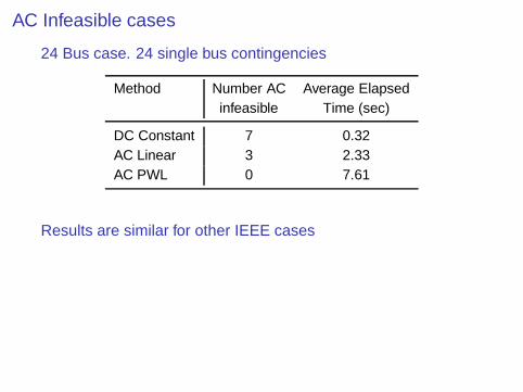
AC Infeasible cases
24 Bus case. 24 single bus contingencies
Method Number AC Average Elapsedinfeasible Time (sec)
DC Constant 7 0.32AC Linear 3 2.33AC PWL 0 7.61
Results are similar for other IEEE cases

Dynamic instability
◮ Islanding creates a shock that could excite dynamic instability,and so prevent the system converging to the planned steadystate.
◮ Tests of previous 452 islanding solutions using 2nd order modelsshowed 14 to be transiently unstable.
◮ Penalise line and generator disconnections to reduce shock
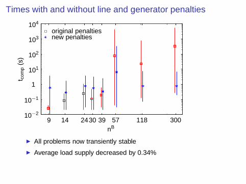
Times with and without line and generator penalties
nB
t com
p(s
)
original penaltiesnew penalties
9 14 2430 39 57 118 30010−2
10−1
1
101
102
103
104
◮ All problems now transiently stable
◮ Average load supply decreased by 0.34%

Transient dynamics 24 Bus
Note different scales
Time (s)
δr g−
δr s,0
(deg
)
0 1 2 3 4 5 6−200
0
200
400
600
800
1000
1200
1400
Time (s)
δr g−
δr s,0
(deg
)
0 1 2 3 4 5 6 7 8−30
−20
−10
0
10
20
30
40
Low penalty - Unstable High penalty - StablePredicted load supplied Predicted load supplied
= 2707 MW = 2675 MW25 generators lose synchrony No loss of synchrony
— all in “safe” section

Current & Future
◮ Scale up: We can solve “2500” bus Polish networks with DC MILP
◮ Computation: Develop heuristics and aggregation methods
◮ Bus splitting: to give more flexibility in islanding.
◮ Dynamic stability: Incorporate more realistic indicators in MILP— using work being done at Durham.
Thank You
Questions?