minimizing landscape resistance for habitat conservation...

Minimizing Landscape Resistance for Habitat

Conservation

CPAIOR 2017

Diego de Una, Graeme Gange, Peter Schachte and Peter J. Stuckey

June 6, 2017

University of Melbourne — CIS Department

Table of Contents

1. Motivation

2. Isolation by Resistance

3. Modeling the Problem

4. Solving the Problem

Diego de Una Minimizing Landscape Resistance CPAIOR2017 2

Motivation

Why did the chicken cross the road?

• Repeatedly shown that isolationleads to extinction.

• Direct perturbation may not lead

to extinction, but isolation does

(Brook et al., 2008).

• Landscape influences genetic

variation (Manel et al., 2003),

(Rosenberg et al., 1997), (Pimm

et al., 1988)

• Action needed to restore to

movement/spread of speciesFragmentation of habitats


Gene Flow Matters

• The Great Prairie Chicken (Westemeier

et al., 1998)

• Threatened Species

• Individuals:

1933 7−→ 25000, 1993 7−→ 50

• Hatching success rate:

1960 7−→ 90%, 1990 7−→ 74%

• Genetic variation declined 30%

(1960-1990)

• Introducing groups from other areas:

Hatching success rate 94%

• Deer Mouse (Schwartz et al., 2005)

• Study compare survival rates:

• Control group 7−→ 88%

• Migrant group introduced 7−→ 98%

Great Prairie Chicken

Deer Mouse


Isolation by Resistance

Modeling Movement of Species via Genetic Distance

• Model for genetic distance (a.k.a.

population differentiation, “fixation

index”, FST ).

• Better understanding of movement of

species

• Better action planning to improve survival

• Metrics (R2 “fit the data”):

• IBD: Geographic distance (0.24)

• LCP/LCC: “Shortest” path (0.37)

• IBR: Effective resistance in an electrical

circuit (0.68)Fig. 1: Comparison of models and how

the fit the data (McRae et al., 2007).


Optimization Problem

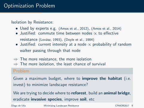
Isolation by Resistance:

• Used by experts e.g. (Amos et al., 2012), (Amos et al., 2014)

• Justified: commute time between nodes ∝ to effective

resistance (Lovasz, 1993), (Doyle et al., 1984)

• Justified: current intensity at a node ∝ probability of random

walker passing through that node

⇒ The more resistance, the more isolation⇒ The more isolation, the least chance of survival

Problem

Given a maximum budget, where to improve the habitat (i.e.

invest) to minimize landscape resistance?

We are trying to decide where to reforest, build an animal bridge,

eradicate invasive species, improve soil, etc


Modeling the Problem

Modeling landscape as an electrical circuit (1)

• Split landscape into “patches”

• Land patches ←→ nodes

• Adjacent patches ←→ resistor

• The value of each resistor is the

“difficulty” of movement between patches

• Eff. res. depends on all the resistors

• Decrease the value of resistors

=⇒ Eff. res. decreases

=⇒ Which resistors matter most?

s

1A

t

Fig. 2: Modeling landscape as a resistor

network (habitats are s and t)



Fig. 3: Example of landscape: current (left) and conductivity (right)

Definitions

Effective Resistance between s and t : Rst

Conductance = 1/Resistance (G = 1/R)

Intensity at a node n =∑

b∈branches(n) |ib|/2Diego de Una Minimizing Landscape Resistance CPAIOR2017 12


Fig. 4: Example of landscape: current (left) and conductivity (right)

More than 2 habitats

We define the total resistance as the sum of all-pairs resistances.


Problem Formulation

Given:

• Graph G = (V ,E ).

• Set of pairs of “focal” nodes F ⊂ V 2.

• Conductance function g∅ : E 7→ R for original resistors.

• Conductance function gE : E 7→ R for improved resistors.

• Budget B.

• Cost function c : E 7→ R for the cost of improving a resistor e.

Minimize the Total Effective Resistance, subject to:

•∑

e∈E[

be︸︷︷︸Boolean decisions for investment

∗ c(e)]≤ B


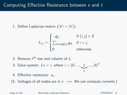
Computing Effective Resistance between s and t

1. Define Laplacian matrix (|V | × |V |):

Li ,j =

−gij if (i , j) ∈ E∑

k∈adj(i) gik if i = j

0 otherwise

2. Remove tth row and column of L.

3. Solve system: Lv = i , where i = (0, ..., 1︸︷︷︸is

, ..., 0)T

4. Effective resistance: vs .

(5. Voltages of all nodes are in v =⇒ We can compute currents.)


Mathematical Problem Formulation

Two habitats:1. Define Laplacian matrix:

Li ,j =

−(be ∗ gE

ij + (1− be) ∗ g∅ij ) if (i , j) ∈ E∑

k∈adj(i)(be ∗ gEik + (1− be) ∗ g∅

ik) if i = j

0 otherwise

2. Remove tth row and column of L.

3. Minimize vs subject to the system:

Lv = i , where i = (0, ..., 1︸︷︷︸is

, ..., 0)T .

Three or more habitats:• Define a system Lv = i for each pair of 〈si , ti 〉 ∈ F .

• Minimize∑

〈si ,ti 〉∈F v〈si ,ti 〉si


Solving the Problem

Solving as a MIP problem

• IBM CPLEx 12.4

• Use indicator constraints of the form:

be =⇒ ge = gE (e)

¬be =⇒ ge = g∅(e)

Problem:

• Weak relaxation

• Optimality gap above 40% even afte 5 hours for 10×10 grids

• Could not find better model (model is “imposed” limited by

the definition of effective resistance)


Greedy algorithm

1. Define the Laplacians for each pair 〈si , ti 〉 ∈ F using g∅.

2. Solve all the systems (No decisions)

3. Compute currents of all branches:

iab = g∅ab ∗

∑〈si ,ti 〉∈F (v

〈si ,ti 〉b − v

〈si ,ti 〉a )

4. Invest in the branches with highest current (more animals

walking through there!) until exhausting the budget.

• Surprisingly good results

• Total resistance dropped between 40% and 60% (for small

landscapes)!


Local Search

1. Begin with the solution s given by the Greedy algorithm.

2. Repeat:

2.1 Choose some “invested resistors” to disinvest (get some

budget back).

2.2 Choose some “uninvested resistors” to invest (exhaust the

budget).

2.3 Compute objective function.

2.4 Accept new solution snew with probability e−(snew−s)

T (simulated

annealing). Update s consequently.

2.5 Update temperature T : less and less likely to accept a worse

solution.


Choosing where we don’t want to invest anymore

• InvRand: Random resistors.

• InvLC: Resistors with least current through them.

• InvLCP: Probability that favors choosing resistors with low

current:

Pr(e) = 1current(e)

Intuition: places where animals aren’t walking anyway.


Choosing new places to invest

• WilRand: Random resistors

• WilBFS: Choose a node with a probability distribution that

favors high current nodes. Perform BFS around that node

until exhausted budget. ⇒ Investments are near each other.

=⇒ Stronger effect in dropping resistance in that region

• WilHC: Choose resistors with highest current.

• WilHCP: Probability that favors choosing high current

resistors.

Intuition: places where animals are walking and it could be made

easier.

Catch: WilHC + InvLC can get stuck in local minimum =⇒do one iteration of WilHCP.Diego de Una Minimizing Landscape Resistance CPAIOR2017 22

Experimental setting

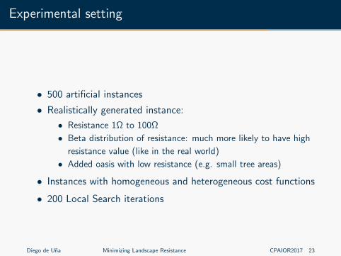
• 500 artificial instances

• Realistically generated instance:

• Resistance 1Ω to 100Ω

• Beta distribution of resistance: much more likely to have high

resistance value (like in the real world)

• Added oasis with low resistance (e.g. small tree areas)

• Instances with homogeneous and heterogeneous cost functions

• 200 Local Search iterations


Results

Averages of the ratios of updated resistance over original resistanceCost

TypeSize

Budget

RatioHabitats Greedy

InvLC InvLCP

WilBFS WilHC WilHCP WilBFS WilHC WilHCP

Homo 20×20 0.11 2 0.30 0.24 0.25 0.25 0.29 0.26 0.27

Homo 25×25 0.09 2 0.30 0.22 0.23 0.24 0.28 0.24 0.26

Homo 25×25 0.09 3 0.38 0.29 0.30 0.29 0.37 0.31 0.35

Homo 30×30 0.07 2 0.37 0.26 0.27 0.28 0.35 0.29 0.31

Homo 30×30 0.07 3 0.42 0.33 0.33 0.33 0.42 0.35 0.41

Homo 50×50 0.04 2 0.44 0.34 0.35 0.36 0.44 0.37 0.40

Homo 50×50 0.04 3 0.48 0.42 0.40 0.41 0.48 0.43 0.48

Homo 50×50 0.04 4 0.52 0.46 0.44 0.45 0.52 0.47 0.52

Homo 100×100 0.02 2 0.49 0.39 0.38 0.41 0.42 0.39 0.37

Homo 100×100 0.02 3 0.53 0.42 0.43 0.42 0.53 0.42 0.50

Homo 100×100 0.02 4 0.55 0.49 0.47 0.46 0.55 0.49 0.55

Homo 100×100 0.02 5 0.58 0.49 0.46 0.50 0.58 0.48 0.58

Rand 20×20 0.11 2 0.44 0.34 0.34 0.38 0.39 0.35 0.40

Rand 25×25 0.09 2 0.45 0.33 0.32 0.36 0.39 0.33 0.38

Rand 25×25 0.09 3 0.53 0.41 0.39 0.38 0.47 0.40 0.44

Rand 30×30 0.07 2 0.52 0.45 0.42 0.44 0.51 0.45 0.48

Rand 30×30 0.07 3 0.57 0.53 0.51 0.52 0.57 0.52 0.56

Rand 50×50 0.04 2 0.56 0.54 0.51 0.53 0.56 0.53 0.56

Rand 50×50 0.04 3 0.60 0.59 0.55 0.58 0.60 0.58 0.60

Rand 50×50 0.04 4 0.63 0.62 0.60 0.63 0.63 0.62 0.63

Rand 100×100 0.02 2 0.61 0.51 0.53 0.52 0.66 0.61 0.65

Rand 100×100 0.02 3 0.64 0.59 0.57 0.60 0.63 0.60 0.64

Rand 100×100 0.02 4 0.65 0.58 0.60 0.62 0.62 0.61 0.64

Rand 100×100 0.02 5 0.68 0.60 0.59 0.62 0.63 0.62 0.65


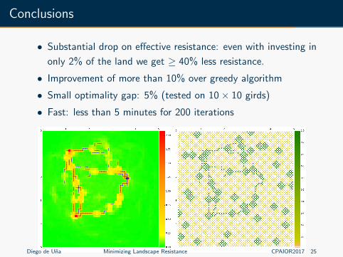
Conclusions

• Substantial drop on effective resistance: even with investing in

only 2% of the land we get ≥ 40% less resistance.

• Improvement of more than 10% over greedy algorithm

• Small optimality gap: 5% (tested on 10× 10 girds)

• Fast: less than 5 minutes for 200 iterations


Thank you for your attention.

Questions?


Comparison (Original: 53.78Ω, Final: 23.03Ω; 100/4900)


Proof of NP-hardness

The STP: Given a graph G = (N,E ), a set R ⊆ N, weighting function w on the

edges and positive integer K , is there a subtree of G weight ≤ K containing the set

of nodes in R? Reduction:• The electric circuit is the graph G .

• The cost function is w .

• The original resistance of edges is infinite (i.e. g∅(e) = 0,∀e ∈ E ).

• The resistance upon investment of all edges is 1 (i.e. gE (e) = 1,∀e ∈ E ).

• The budget is K .

• The set of pairs of focal nodes F is the set of all pairs of distinct nodes in R,

which can be built in O(|R|2).Assume we have an algorithm to solve the landscape problem that gives a solution

S . By investing in the selected edges S we obtain a resistance RS ∈ R iff there is

enough budget K , and RS =∞ otherwise:1. If RS =∞, there is no Steiner Tree of cost ≤ K , since we could not connect

focal nodes with 1Ω resistors.

2. If RS = 0, G∗ = G \ invested(S). G∗ is of cost ≤ K and a subgraph of G that

connects all nodes in R pairwise. G∗ contains/is a Steiner Tree.Diego de Una Minimizing Landscape Resistance CPAIOR2017 28

MIP model

Minimize

|F |∑i=1

v〈si ,ti 〉si

s.t.

e=|E |∑e=0

bec(e) ≤ B

∀〈si , ti 〉 ∈ P, ∀x ∈ N\si , ti,∑

y∈adj(x)

p〈si ,ti 〉(x ,y),x −

∑y∈adj(x)\ti

p〈si ,ti 〉(x ,y),y = 0

∀〈si , ti 〉 ∈ P,∑

y∈adj(si )

p〈si ,ti 〉(si ,y),si

−∑

y∈adj(si )\ti

p〈si ,ti 〉(si ,y),y = 1

∀〈si , ti 〉 ∈ P, ∀e = (x , y) ∈ E ,∀z ∈ x , y,

p〈si ,ti 〉e,z = beg

E (e)v〈si ,ti 〉z + (1− be)g∅(e)v

〈si ,ti 〉z


Minimize the sum of voltages at the

source habitats

MIP model

Minimize

|F |∑i=1

v〈si ,ti 〉si

s.t.

e=|E |∑e=0

bec(e) ≤ B

∀〈si , ti 〉 ∈ P, ∀x ∈ N\si , ti,∑

y∈adj(x)


∑y∈adj(x)\ti

p〈si ,ti 〉(x ,y),y = 0

∀〈si , ti 〉 ∈ P,∑

y∈adj(si )


−∑

y∈adj(si )\ti

p〈si ,ti 〉(si ,y),y = 1

∀〈si , ti 〉 ∈ P, ∀e = (x , y) ∈ E ,∀z ∈ x , y,



〈si ,ti 〉z


Budget constraint

MIP model

Minimize

|F |∑i=1

v〈si ,ti 〉si

s.t.

e=|E |∑e=0

bec(e) ≤ B

∀〈si , ti 〉 ∈ P, ∀x ∈ N\si , ti,∑

y∈adj(x)


∑y∈adj(x)\ti

p〈si ,ti 〉(x ,y),y = 0

∀〈si , ti 〉 ∈ P,∑

y∈adj(si )


−∑

y∈adj(si )\ti

p〈si ,ti 〉(si ,y),y = 1

∀〈si , ti 〉 ∈ P, ∀e = (x , y) ∈ E ,∀z ∈ x , y,



〈si ,ti 〉z


All non-focal nodes need

to maintain a flow of

current equal 0

MIP model

Minimize

|F |∑i=1

v〈si ,ti 〉si

s.t.

e=|E |∑e=0

bec(e) ≤ B

∀〈si , ti 〉 ∈ P, ∀x ∈ N\si , ti,∑

y∈adj(x)


∑y∈adj(x)\ti

p〈si ,ti 〉(x ,y),y = 0

∀〈si , ti 〉 ∈ P,∑

y∈adj(si )


−∑

y∈adj(si )\ti

p〈si ,ti 〉(si ,y),y = 1

∀〈si , ti 〉 ∈ P, ∀e = (x , y) ∈ E ,∀z ∈ x , y,



〈si ,ti 〉z


The source has a flow of 1

MIP model

Minimize

|F |∑i=1

v〈si ,ti 〉si

s.t.

e=|E |∑e=0

bec(e) ≤ B

∀〈si , ti 〉 ∈ P, ∀x ∈ N\si , ti,∑

y∈adj(x)


∑y∈adj(x)\ti

p〈si ,ti 〉(x ,y),y = 0

∀〈si , ti 〉 ∈ P,∑

y∈adj(si )


−∑

y∈adj(si )\ti

p〈si ,ti 〉(si ,y),y = 1

∀〈si , ti 〉 ∈ P, ∀e = (x , y) ∈ E , ∀z ∈ x , y,



〈si ,ti 〉z

Diego de Una Minimizing Landscape Resistance CPAIOR2017 33The value of each product depends on the investments

minimizing landscape resistance for habitat conservation...

Documents