Minimizing Flight Delay

Tanujit Dey∗, David Phillips†, Patrick Steele‡

Abstract

In this paper, we model the problem of finding the minimum-delay route as a shortest pathproblem with stochastic costs. Our solution algorithm uses Monte Carlo simulation and networkoptimization techniques. Of particular novelty in our approach is the air network sampling that weuse in order to accurately model the cascading effect of delays on flights. Our statistical models andsimulations are based on real flight data obtained from the U.S. Department of Transportation.

Key Words: bootstrapping and ensemble regression, stochastic optimization, data mining, networkoptimization

1. Introduction

Air traffic delays are a current and growing problem with severe economic and environ-mental impacts. A recent congressional report has estimated that delays cost $41 billion in2007 alone and caused an extra 740 million gallons of jet fuel to be burned (Schumer andMaloney, 2008). Moreover, a 2009 Government Accounting Office report has estimatedthat the number of flights is going to increase from 50 million in 2008 to 80 million bythe year 2025 (Dillingham, 2009). We consider the problem of the air traveler determininghow to best plan his travel.

Our specific contributions are as follows.

• We formulate the problem of finding a flight plan with minimum delay as a mathe-matical program we call the shortest paths problem with correlated random lengths.We also show how to extend our formulation to minimize more general functionssuch as overall flight time and flight costs.

• We develop a statistical model by using an ensemble technique to find significantvariables for predicting delay for any given airline. The resulting prediction can thenbe used in cascade sampling.

• We give an algorithm to determine the relevant flight legs for the given origin anddestination. Subsetting to the relevant flight legs allows us to tractably use MonteCarlo simulation in computing the flight plans with the highest probability of smalldelay.

• We implemented a visualization tool which displays results from our algorithms aswell as other statistical analyses on the air transport graph. The visualization ofboth our algorithmic results and the statistical analyses makes it possible to discernmeaningful trends in a large and complicated dataset.

∗Mathematics Department, The College of William & Mary, tdey@wm.edu. Supported in part by NSFgrant DMS-0703532 and a William & Mary summer grant

†Mathematics Department, The College of William & Mary, djphil@wm.edu. Supported in part by NSFgrant DMS-0703532 and a NASA/VSGC New Investigator grant

‡Mathematics Department, The College of William & Mary, prsteele@wm.edu. Supported in part bya Chappell fellowship.

IAD LAX PHF

DFW BOS

2

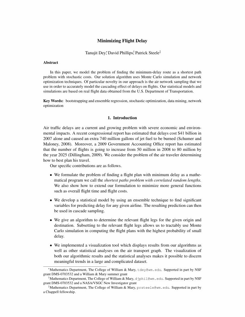
Figure 1: Two airport-flight graphs on 5 airports, represented as nodes, with 9 flightsrepresented as edges. Note that the edge (DFW,BOS) is not the same as (BOS,DFW). Theedges in red are on the path (IAD,BOS), (BOS,DFW), (DFW,BOS), (BOS,LAX)

Previous works focus on the scheduling decisions airlines can make to reduce overalldelay. For example, Bratu and Barnhart (2006) solve integer programs that help airlinecompanies determine flight rerouting plans that minimize the delay to passengers whenexogenous events (e.g., inclement weather) disrupt the flight schedule. Delahaye and Odoni(1997) use stochastic optimization techniques to determine air traffic policies that reduceair space congestion. In related papers, Nilim et al. (2003) and Nilim and El Ghaoui (2005)present Markov decision process approaches to scheduling flights accounting for inclementweather.

In contrast, we focus on developing decision support tools that help individual travelersfind flight plans that minimize expected delay. In formulating and solving the problem fromthe individual traveler’s perspective our methods can also be used by airlines and air trafficpolicy makers to determine bottleneck airports with respect to delay.

An essential part of our model is the use of the airport-flight graph. We consider agraph, G = (V, E), where V represents vertices and E represents edges between pairsof vertices. An edge (i, j) ∈ E implies that the edge “starts” at the node i and “ends”at node j. By considering the airports as vertices and the flight legs as edges, a graphis a natural way to represent the air travel system (all references cited that consider airtravel use variations of this model), e.g., see Figure 1. A flight plan in such a graph cor-responds to a path in the network, which can be defined as a sequence of edges, P =(i1, i2), (i2, i3), . . . , (ik−1, ik)where every consecutive pair of edges share a vertex (e.g.,again, see Figure 1) and no edge repeats itself.1

The organization of the article is as follows. The description of the data is in Section1.1 and the statistical models and simulation are in Section 2. The outputs of the simulationform the inputs to the delay minimization formulation which we describe in Section 3. Wepresent our algorithms to conduct the simulation and solve the delay minimization problemin Section 4. Computational experiments are discussed in Section 5. Proofs of our resultsare omitted in this extended abstract for space reasons and available in Dey et al. (2009).

1.1 Data

The data set used came from the U.S. Department of Transportation’s Bureau of Trans-portation Statistics, and includes data on domestic flights from 1987 to 2008. Each flighthas a database entry that includes information about the arrival, departure and delay times,

1We only consider directed edges and paths.

DelayLevel 0 1 2 3 4

Sum of all delays (minutes) 0− 15 15− 30 30− 60 60− 120 120+

Table 1: The response variable DelayLevel.

origin and destination airports and carrier. The data set contains close to 120 million flightsand is over 12 gigabytes large.

We analyzed a subset of a data that consisted of the largest seven carriers in terms ofnumber of flights, which were American Airlines (AA), Continental Airlines (CO), DeltaAirlines (DL), Southwest Airlines (WN), American Eagle Airlines (MQ), United Airlines(UA), and SkyWest (OO) Airlines. Within these airlines, we analyzed 1987, 1992, 1997,and 2002 for trends over time, and constructed our regression models and simulation usingthe years 2005 to 2008. The variables we used were year, month, day of month, day ofweek, departure time, and arrival time of each flight, the carrier, the departure, arrival,weather, NAS, security, taxi in, taxi out, and late aircraft delays, and finally the origin anddestination of the flight. Cancelled flights were omitted from the analysis.

2. Data analysis & simulation

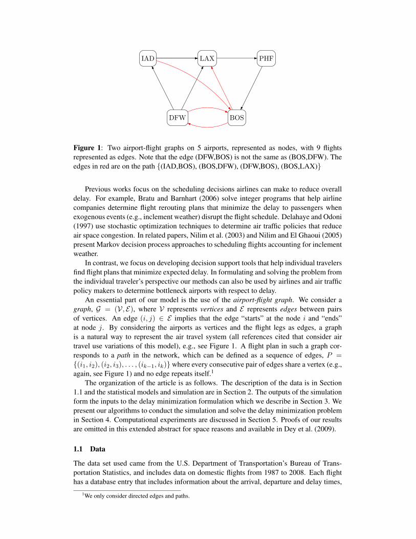
Given the size of the data set and the time length over which the data spans, we choose tofocus our analyses on recent data in order to best predict delay for current flights. We did,however, examine simple statistics from 1987, 1992, 1997 and 2002 in order to demonstratehow subtle differences in the air network graph can reveal information about the underlyingdata. As Figure 2 shows, the increased complexity of the air network can be seen withairport graphs. Other trends such as an evolution to a “hub-and-spokes” air network canalso be seen.

We describe our statistical model for predicting delay in Section 2.1 and our simulationfor generating delay in Section 2.2.

2.1 Statistical Model

The objective of our statistical analysis was to create an accurate model for predicting delay.Because of the characteristics of our data, we used a full multiple linear regression model,and in order to obtain a stable predictor, we used ensemble estimates via bootstrapping.

Due to the small number of variables relative to the sheer size of the data, we fitteda full model for multiple linear regression, and then selected the significant variables forpredicting delay. There were several delay variables that corresponded to different types ofdelay. In order to use both the type and the magnitude of each type of delay as a predictorfor a given day, we created the categorical variable DelayLevel, which is based on the sumof all the different delays, and is defined in Table 1.

In order to obtain a stable estimator, we used a bootstrapping technique. For eachbootstrap draw, a multiple linear regression was performed on 70% of the data (sampledwithout replacement). The significant variables and their corresponding estimates wereselected. These are then combined over the bootstrap draws to form an ensemble estimatorfor each given airline/year. By introducing bootstrapping, we injected extra randomnessinto the data that gets averaged over all the bootstrap runs which results in a estimator thatis stable.

United Airlines1987 2008

Figure 2: Historical delay averages for United Airlines in 1987 and 2008 are presentedin two different graph depictions. In both graphs, the color indicates the average delay perflight leg. The top row has “edge”-focused graphs where the actual number of flights can beobserved. Note that both the 1987 and 2008 arc graphs have the same connectivity but thatexpected delay has increased. The bottom row shows the “node”-focused graphs where thenode size corresponds to number of flights and the node opacity indicates the probability ofdelay. The node focused graph shows how United has converted to the “hub-and-spokes”airport graph model

Conceptually, the method can be explained as the following multi-stage procedure:

1. Bootstrap the data. Run multiple regression on the bootstrapped data.

2. Find the significant variables and their corresponding estimates based on the outputof step 1.

3. Repeat steps 1-2.

4. After finishing the bootstrap iterations, calculate an ensemble estimator for each sig-nificant variables in the model.

2.2 Simulation

In this section we describe our simulation. Our goal in the simulation was to accuratelygenerate delay for each flight leg in a way which (a) is stable, (b) takes into account theimpact of delays from the rest of the system and (c) is computationally efficient. In all ofour simulations, we first determine the flight legs that are relevant to the desired flight plan.For example, if the flight plan is to travel from JFK to LAX on a Monday in Novemberusing Delta in 2 flights or less, we first must find all Delta flight legs that would allow

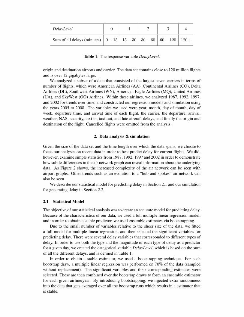
American Airlines, Albuquerque, NM to Jackson Hole, WYNaive Cascade

Figure 3: Line thickness indicates probability of being the shortest delay path. Colorindicates the expected delay in minutes. Naive sampling indicates that both of the twoflight plans have an equal probability of being the shortest delay path, whereas Cascadesampling indicates that flying through DFW has a much greater likelihood of being theshortest delay path.

a traveler to start from JFK and end up in LAX on a Monday in November within twoflight legs. Determining the subset of relevant flight legs is nontrivial and we describethis fully in Section 4. We then sample variables from the generated subset in order tocalculate predicted delay. We devised two sampling methods, labeled Naive and Cascade,and two ways of using the sampled variables calculate predicted total delay, labeled Actualand Ensemble. Thus, there were a total of four different simulations. As we shall see,our preferred sampling method was Cascade-Ensemble. We first describe the differencethe different sampling methods and then the difference between calculated predicted totaldelay.

In Naive sampling, the data for each flight leg is chosen independently and uniformlyat random from the relevant data. Continuing the JFK to LAX example, suppose that arelevant flight leg was JFK to ORD. In Naive sampling, we uniformly select a flight atrandom from amongst all Delta JFK-ORD flights that occurred on a Monday in Novemberfrom 2005 to 2008. Assuming that ORD-LAX was also relevant, the ORD-LAX flight legpredictor variables used would be independently and uniformly chosen at random from allDelta ORD-LAX flights that also occurred on a Monday in November from 2005 to 2008.Note that Naive sampling does not take into account interdependencies between flight legs,nor does it necessarily sample flights that are actually feasible to the travel plan if morethan one flight leg is required.

In Cascade sampling we seek to address the flight-leg interdependencies and flightplan feasibility requirements. Instead of sampling flight legs independently, we sample aday uniformly from amongst the appropriate days of travel. Within the sampled day, theflight legs sampled must satisfy the feasibility constraint that they leave no sooner than theincoming flight leg arrives. In our previous example, if Cascade sampling was used, firsta date would be chosen from all the Mondays of November from 2005 to 2008. Then,starting at JFK, a Delta JFK-ORD flight leg would be uniformly chosen at random. Then,the ORD-LAX flight would be uniformly chosen at random from all flights that took offafter the JFK-ORD flight landed. Note that Cascade sampling generates flight plans thatcould actually occur within the desired dates. Also, Cascade sampling accurately modelsthe correlations of delay that occur between flight legs by realistically generating the typesof acute delay-causing events that occur in the airport system. As shown in Figure 3,

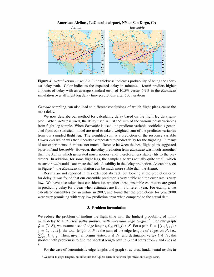
American Airlines, LaGuardia airport, NY to San Diego, CAActual Ensemble

Figure 4: Actual versus Ensemble. Line thickness indicates probability of being the short-est delay path. Color indicates the expected delay in minutes. Actual predicts higheramounts of delay with an average standard error of 10.5% versus 6.9% in the Ensemblesimulation over all flight leg delay time predictions after 500 iterations.

Cascade sampling can also lead to different conclusions of which flight plans cause themost delay.

We now describe our method for calculating delay based on the flight leg data sam-pled. When Actual is used, the delay used is just the sum of the various delay variablesfrom flight leg sample. When Ensemble is used, the predictor variable coefficients gener-ated from our statistical model are used to take a weighted sum of the predictor variablesfrom our sampled flight leg. The weighted sum is a prediction of the response variableDelayLevel which was then linearly extrapolated to predict delay for the flight leg. In manyof our experiments, there was not much difference between the best flight plans suggestedbyActual and Ensemble. However, the delay prediction from Ensemble was much smootherthan the Actual which generated much noisier (and, therefore, less stable) fits to the pre-dictors. In addition, for some flight legs, the sample size was actually quite small, whichmeans Actual would exacerbate the lack of stability in the delay prediction. As can be seenin Figure 4, the Ensemble simulation can be much more stable than the Actual.

Results are not reported in this extended abstract, but looking at the prediction errorfor delay, it was found that our ensemble predictor is very stable and the error rate is verylow. We have also taken into consideration whether these ensemble estimators are goodin predicting delay for a year when estimates are from a different year. For example, wecalculated ensembles for an airline in 2007, and found that the predictions for year 2008were very promising with very low prediction error when compared to the actual data.

3. Problem formulation

We reduce the problem of finding the flight time with the highest probability of mini-mum delay to a shortest paths problem with uncertain edge lengths.2 For our graphG = (V, E), we assume a set of edge lengths, `ij ,∀(i, j) ∈ E . For a path P = (ij , ij+1) :j = 1, . . . , k, the total length of P is the sum of the edge lengths of edges on P , i.e.,∑k

j=1 `ijij+1 . Then, given an origin vertex, s ∈ N , and destination vertex t ∈ N , theshortest path problem is to find the shortest length path in G that starts from s and ends att.

For the case of deterministic edge lengths and graph structures, fundamental results in2We refer to edge lengths, but note that the typical term in network optimization is edge costs.

shortest paths algorithms were given by Bellman (1958) and Dijkstra (1959). Their workis particularly noteworthy since variants of their algorithms are still the fastest known al-gorithms for solving the deterministic shortest paths problems over general (Bellman) andnonnegative (Dijkstra) edge lengths. The subsequent work on shortest paths problems isextensive, and for space reasons, we refer readers toAhuja et al. (1993) and Cormen et al.(2001) for several algorithms on the deterministic case. Early work on the case where theedge lengths were randomized include Dijkstra (1959) where the problem was reduced tothe deterministic version by considering expected values of each edge lengths. For theproblem where edge lengths were random, but independently generated, algorithms thatfind edges with probability guarantees include those by Loui (1983) and adaptive algo-rithms by Bertsekas and Tsitsiklis (1991) and Fan and Nie (2006). For the case where edgelengths were random and correlated but the density functions were known, Fan et al. (2005)recently described an algorithm to determine the path with the highest probability of beingless than a certain length. Our problem differs from these previous results in that our prob-ability density functions are unknown, although we are able to simulate the various edgelengths. Moreover, since the delay of a given flight leg causes delays to other flight legs,we cannot assume independence in flight delays.

Recall that G = (V, E) is a graph where V are vertices representing airports and Eare edges (i.e., pairs of nodes) that represent possible flight legs. We use Lij to denotethe random amount of delay on a given flight leg (i, j) ∈ E . For a given origin, s, anddestination, t, we denote the set of paths from s to t in G as Ω. We wish to find αP , whichis the probability that P ∈ Ω represents the flight plan with the greatest probability of thelowest delay. To find this, we can solve the following stochastic mathematical program.

min∑

P∈Ω(∑

(i,j)∈P Lij)αP

subject to∑

P∈Ω αP = 1∀P ∈ Ω, αP ≥ 0.

(1)

We note that to solve even a deterministic version (i.e., when Lij are constant) of (1)is complicated since the size of Ω is exponential in the number of edges. However, we canreformulate (1) by considering arc flows, xij , which represent the probability that (i, j) ison some path that has the probability of being the minimum delay path.

min∑

(i,j)∈E Lijxij

subject to 0 ≤ xij ≤ 1 ∀(i, j) ∈ E(a)

∑j:(i,j)∈E xij −

∑k:(k,i)∈E xki = 0 ∀i ∈ V \ s, t

(b)∑

j:(s,j)∈E xsj = 1(c)

∑k:(k,t)∈E xkt = 1

(2)

Constraints (a) ensure that flow going into any vertex leaves the vertex, except for theorigin and destination. In the context of our model, this ensures that the traveler leaves anyairport she arrives at unless it’s the origin or destination. Constraint (b) ensures the travelerleaves the origin and constraint (c) ensures the traveler arrives at the destination.

To convert an arc flow solution, xij , to a path solution, αij , we can use a flow decom-position algorithm (Ahuja et al., 1993). Such an algorithm runs in time that is linear inproportion to the number of edges. We note that the formulations are easily extended torandom variables other than Lij , such as total travel time and travel cost.

To solve for xij in (2), we adopt a Monte Carlo simulation (Spall, 2005). For eacharc, we randomly generate a sample length and then we solve a (deterministic) shortestpaths problem. By repeating this several times, and counting up the number of times anarc appears on a shortest path, we can estimate xij with a controllable sample. Here is apseudo-code description of our approach.

(a) Construct a relevant network, G = (V, E), for the given origin, destination, flightdate, airline(s) and number of flight legs.

(b) Initialize arc counters cij to zero for each (i, j) ∈ E .

(c) Repeat steps (d)-(f) k times

(d) Generate valid flight delays to find sample realizations of Lij for all (i, j) ∈ E .

(e) Find the shortest path with respect to the sample realizations.

(f) For all arcs (i, j) on the shortest path found, increment cij by 1.

(g) Set xij = cij/k and return the xij .

To solve for the shortest path problem with the sample realizations in step (d), we useDijkstra’s algorithm since we assume the flight delays (i.e., arc lengths) to be nonnegative.We could relax this assumption and use Bellman’s algorithm instead. Accomplishing step(a) is complicated, and we describe our algorithms to construct the network in Section 4.

4. Constructing and visualizing graphs

In this section, we first describe our algorithm for subsetting our flight network G to theairports (i.e., vertices) and flight legs (i.e., edges) relevant to the origin-destination, airline,date and flight-leg constraint we are interested in. We then describe our visualization tool.

4.1 Constructing relevant graphs

Since our runtime scales with our problem size, we seek to reduce the flight network by asmuch as possible. The network created only contains flight legs that are a part of a pathfrom the origin to the destination. We let k denote the constraint on the number of flightlegs our flight plan is allowed.

To create this network, we begin with the full network and apply an algorithm we callREDUCE. REDUCE subsets the network by selecting only the vertices and edges that satisfythe following conditions. Only airports that can be reached in k flight legs or fewer from theorigin or destination are kept. Then, we only include a flight (i, j) if j is within k− 1 flightlegs of the destination and i is within k−1 flight legs of the origin. To conduct the removalof these flight legs, we use Breadth-First Search on G and on the reverse graph of G, whichis GR = (V, ER) where ER = (i, j) : (j, i) ∈ E. We can accomplish REDUCE using fourpasses of Breadth-First Search. To conclude this section, we state our main result.

Theorem 1. Given a graph G, source node s and destination node t, REDUCE produces agraph that contains only arcs that can be traversed as part of a k-path from the origin nodes to the destination node t, and runs in O(|V|+ |E|) time.

4.2 Visualizing our results

Using a combination of Java, Python and c, we implemented an applet which takes theorigin, destination and flight date. The tool calls our algorithms that sample the data andsolve the stochastic optimization problem. It then draws the subgraph associated with thepaths that had any positive sample probability of being the minimum delay flight plan wherethe arc thickness corresponds to the probability. The tool also color codes arcs to indicatethe degree of expected delay on the different flight legs.

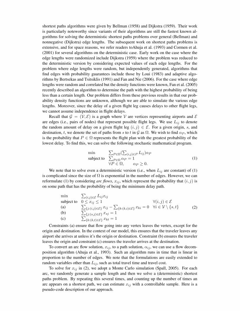
SFO-BTV, United, Mon. in Dec. PHL–PDX, Continental, Wed. in Mar.

IAD–LAS, Delta, Fri. in June SAN–JFK, American, Sun. in Sep.

Figure 5: A variety of flight plans generated with our methods.

5. Experimental results

Our algorithms and models generate stable predictions of flight plans that have smallamounts of delay. As can be seen in Figure 5, our algorithms can generate flight plansfor any possible date, origin and destination on the seven largest air carriers of our dataset.Our algorithms will also work if the data is not specified or a range of dates is specified. Allof our reported results computed 500 iterations of the Monte Carlo simulation on a 3.0 GHzIntel machine with two dual-core processors and 4 GB of RAM. Our algorithms took lessthan minute to find flight plans when no more than 2 flight legs were allowed. However,when 3 flight legs were allowed, the runtime increased to 7 minutes. In future work, weplan on implementing methods that scale more efficiently with the flight leg constraint.

References

Ahuja, R. K., Magnanti, T. L., and Orlin, J. B. (1993), Network Flows : Theory, Algorithms,and Applications, Englewood Cliffs, NJ: Prentice Hall.

Bellman, R. (1958), “On a routing problem,” Quarterly of Applied Mathematics, 16, 87–90.

Bertsekas, D. and Tsitsiklis, J. (1991), “An analysis of stochastic shortest path problems,”Mathematics of Operations Research, 580–595.

Bratu, S. and Barnhart, C. (2006), “Flight operations recovery: New approaches consider-ing passenger recovery,” Journal of Scheduling, 9, 279–298.

Cormen, T. H., Leiserson, C. E., Rivest, R. L., and Stein, C. (2001), Introduction to Algo-rithms, The MIT Press and McGraw-Hill, 2nd ed.

Delahaye, D. and Odoni, A. (1997), “Airspace congestion smoothing by stochastic opti-mization,” Lecture Notes in Computer Science, 163–176.

Dey, T., Phillips, D. J., and Steele, P. (2009), “Minimizing flight delay,” Tech. rep., Dept.of Math, College of William & Mary, contact authors for manuscript.

Dijkstra, E. W. (1959), ““A Note on Two Problems in Connection with Graphs”,” Nu-merische Mathematik, 1, 260–271.

Dillingham, G. (2009), “Next Generation Air Transportation System, Status of Transfor-mation and Issues Associated with Midterm Implementation of Capabilities,” Testimonybefore the Subcommittee on Aiviation, Committee on Transportation and Infrastructure,House of Representatives GAO-09-479T, United States Government Accountability Of-fice, Washington, DC.

Fan, Y., Kalaba, R., and Moore, J. (2005), “Shortest paths in stochastic networks withcorrelated link costs,” Computers and Mathematics with Applications, 49, 1549–1564.

Fan, Y. and Nie, Y. (2006), “Optimal routing for maximizing the travel time reliability,”Networks and Spatial Economics, 6, 333–344.

Loui, R. (1983), “Optimal paths in graphs with stochastic or multidimensional weights,”Communications of the ACM.

Nilim, A. and El Ghaoui, L. (2005), “Robust solutions to markov decision problems withuncertain transition matrices,” Operations Research, 53, 780–798.

Nilim, A., El Ghaoui, L., and Duong, V. (2003), “Multi-Aircraft Routing and Traffic FlowManagement under Uncertainty,” in 5th USA/Europe Air Traffic Management Researchand Development Seminar, Budapest, Hungary, pp. 23–27.

Schumer, C. and Maloney, C. (2008), “Your flight has been delayed again: flight delayscost passengers, airlines, and the US economy billions,” The US Senate Joint EconomicCommittee.

Spall, J. (2005), Introduction to stochastic search and optimization: estimation, simulation,and control, Wiley-Interscience.