Minimax with Alpha Beta Pruning

• The minimax algorithm is a way of finding an optimal move in a two player game. Alpha-beta pruning is a way of finding the optimal minimax solution while avoiding searching subtrees of moves which won't be selected.

• In the search tree for a two-player game, there are two kinds of nodes, nodes representing your moves and nodes representing your opponent's moves.

1

MAX Nodes• Nodes representing your moves are generally

drawn as squares (or possibly upward pointing triangles):

• These are also called MAX nodes. The goal at a MAX node is to maximize the value of the subtree rooted at that node. To do this, a MAX node chooses the child with the greatest value, and that becomes the value of the MAX node.

2

MIN Nodes• Nodes representing your opponent's moves are

generally drawn as circles (or possibly as downward pointing triangles):

• These are also called MIN nodes. The goal at a MIN node is to minimize the value of the subtree rooted at that node. To do this, a MIN node chooses the child with the least (smallest) value, and that becomes the value of the MIN node.

3

• Alpha-beta pruning gets its name from two bounds that are passed along during the calculation, which restrict the set of possible solutions based on the portion of the search tree that has already been seen. Specifically, – β Beta is the minimum upper bound of possible solutions – α Alpha is the maximum lower bound of possible

solutions Thus, when any new node is being considered as a possible path to the solution, it can only work if: where N is the current estimate of the value of the node.

4

• To visualize this, we can use a number line. At any point in time, alpha and beta are lower and upper bounds on the set of possible solution values, like so:

• As the problem progresses, we can assume restrictions about the range of possible solutions based on min nodes (which may place an upper bound) and max nodes (which may place a lower bound). As we move through the search tree, these bounds typically get closer and closer together:

5

• This convergence is not a problem as long as there is some overlap in the ranges of alpha and beta. At some point in evaluating a node, we may find that it has moved one of the bounds such that there is no longer any overlap between the ranges of alpha and beta:

• At this point, we know that this node could never result in a solution path that we will consider, so we may stop processing this node. In other words, we stop generating its children and move back to its parent node. For the value of this node, we should pass to the parent the value we changed which exceeded the other bound.

6

Example: alpha-beta pruning (Slide 7 to 46)Maxnode Minnode

β: minimum upper bound , α maximum lower bound

7

At the start of the problem, you see only the current state (i.e. the current position of pieces on the game board). As for upper and lower bounds, all you know is that it's a number less than infinity and greater than negative infinity. Thus, here's what the initial situation looks like:

8

Since the bounds still contain a valid range, we start the problem by generating the first child state, and passing along the current set of bounds. At this point our search looks like this:

9

We're still not down to depth 4, so once again we generate the first child node and pass along our current alpha and beta values:

10

And one more time:

11

When we get to the first node at depth 4, we run our evaluation function on the state, and get the value 3. Thus we have this:

12

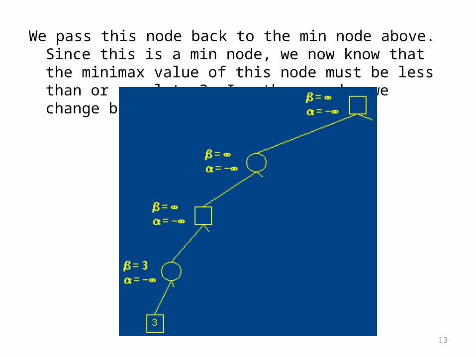
We pass this node back to the min node above. Since this is a min node, we now know that the minimax value of this node must be less than or equal to 3. In other words, we change beta to 3.

13

Note that the alpha and beta values at higher levels in the tree didn't change. When processing actually returns to those nodes, their values will be updated. There is no real gain in proagating the values up the tree if there is a chance they will change again in the future. The only propagation of alpha and beta values is between parent and child nodes.

If we plot alpha and beta on a number line, they now look like this:

14

Next we generate the next child at depth 4, run our evaluation function, and return a value of 17 to the min node above:

15

Since this is a min node and 17 is greater than 3, this child is ignored. Now we've seen all of the children of this min node, so we return the beta value to the max node above. Since it is a max node, we now know that it's value will be greater than or equal to 3, so we change alpha to 3:

16

Notice that beta didn't change. This is because max nodes can only make restrictions on the lower bound. Further note that while values passed down the tree are just passed along, they aren't passed along on the way up. Instead, the final value of beta in a min node is passed on to possibly change the alpha value of its parent. Likewise the final value of alpha in a max node is passed on to possibly change the beta value of its parent.

At the max node we're currently evaluating, the number line currently looks like this:

17

We generate the next child and pass the bounds along:

18

Since this node is not at the target depth, we generate its first child, run the evaluation function on that node, and return it's value:

19

Since this is a min node, we now know that the value of this node will be less than or equal to 2, so we change beta to 2:

20

The number line now looks like this:

As you can see from the number line, there is no longer any overlap between the regions bounded by alpha and beta. In essence, we've discovered that the only way we could find a solution path at this node is if we found a child node with a value that was both greater than 3 and less than 2. Since that is impossible, we can stop evaluating the children of this node, and return the beta value (2) as the value of the node.

21

The 2 alone is enough to make this subtree fruitless, so we can prune any other children and return it.

beta pruning

22

Back at the parent max node, our alpha value is already 3, which is more restrictive than 2, so we don't change it. At this point we've seen all the children of this max node, so we can set its value to the final alpha value:

23

Now we move on to the parent min node. With the 3 for the first child value, we know that the value of the min node must be less than or equal to 3, thus we set beta to 3:

24

Since we still have a valid range, we go on to explore the next child. We generate the max node...

25

... it's first child min node ...

26

... and finally the max node at the target depth. All along this path, we merely pass the alpha and beta bounds along.

27

At this point, we've seen all of the children of the min node, and we haven't changed the beta bound. Since we haven't exceeded the bound, we should return the actual min value for the node. Notice that this is different than the case where we pruned, in which case you returned the beta value. The reason for this will become apparent shortly.

28

Now we return the value to the parent max node. Based on this value, we know that this max node will have a value of 15 or greater, so we set alpha to 15:

29

Now the graph of alpha and beta on a number line looks like this:

30

Once again the alpha and beta bounds have crossed, so we can prune the rest of this node's children and return the value that exceeded the bound (i.e. 15). Notice that if we had returned the beta value of the child min node (3) instead of the actual value (15), we wouldn't have been able to prune here.

alpha pruning

31

Now the parent min node has seen all of it's children, so it can select the minimum value of it's children (3) and return.

32

Finally we've finished with the first child of the root max node. We now know our solution will be at least 3, so we set the alpha value to 3 and go on to the second child.

33

Passing the alpha and beta values along as we go, we generate the second child of the root node...

34

... and its first child ...

... and its first child ...

35

... and its first child. Now we are at the target depth, so we call the evaluation function and get 2:

36

The min node parent uses this value to set it's beta value to 2:

37

Now the graph of alpha and beta on a number line looks like this:

38

Once again we are able to prune the other children of this node and return the value that exceeded the bound. Since this value isn't greater than the alpha bound of the parent max node, we don't change the bounds.

beta pruning

39

From here, we generate the next child of the max node:

40

Then we generate its child, which is at the target depth. We call the evaluation function and get its value of 3.

41

The parent min node uses this value to set its upper bound (beta) to 3:

42

At this point the number line graph of alpha and beta looks like this:

In other words, at this point alpha = beta. Should we prune here? We haven't actually exceeded the bounds, but since alpha and beta are equal, we know we can't really do better in this subtree.

The answer is yes, we should prune. The reason is that even though we can't do better, we might be able to do worse. Remember, the task of minimax is to find the best move to make at the state represented by the top level max node. As it happens we've finished with this node's children anyway, so we return the min value 3.

43

The max node above has now seen all of its children, so it returns the maximum value of those it has seen, which is 3.

44

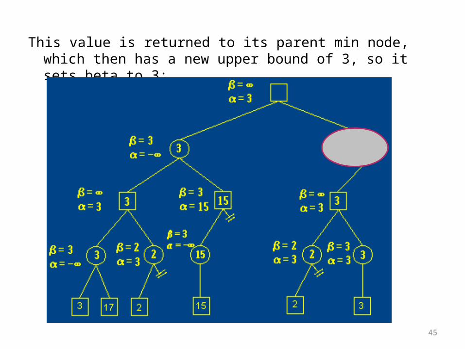
This value is returned to its parent min node, which then has a new upper bound of 3, so it sets beta to 3:

45

Now the graph of alpha and beta on a number line looks like this:

Once again, we're at a point where alpha and beta are tied, so we prune. Note that a real solution doesn't just indicate a number, but what move led to that number.

46

Alpha Beta Properties

• Pruning does not affect final result• Good move ordering improves effectiveness

of pruning• With perfect ordering, time complexity is

O(bm/2)

47

Status of AI Game Players• Tic Tac Toe

– Tied for best player in world• Othello

– Computer better than any human– Human champions now refuse to play

computer• Scrabble

– Maven beat world champions Joel Sherman and Matt Graham

• Backgammon– 1992, Tesauro combines 3-ply search &

neural networks (with 160 hidden units) yielding top-3 player

• Bridge– Gib ranked among top players in the

world

• Poker– Pokie plays at strong intermediate level

• Checkers– 1994, Chinook ended 40-year reign of

human champion Marion Tinsley• Chess

– 1997, Deep Blue beat human champion Gary Kasparov in six-game match

– Deep Blue searches 200M positions/second, up to 40 ply

– Now looking at other applications (molecular dynamics, drug synthesis)

• Go– 2008, MoGo running on 25 nodes (800

cores) beat Myungwan Kim– $2M prize available for first computer

program to defeat a top player

48