minimal webs in riemannian manifolds
TRANSCRIPT

Geom Dedicata (2008) 133:7–34DOI 10.1007/s10711-008-9230-8
ORIGINAL PAPER
Minimal webs in Riemannian manifolds
Steen Markvorsen
Received: 29 August 2002 / Accepted: 3 January 2008 / Published online: 23 January 2008© Springer Science+Business Media B.V. 2008
Abstract For a given combinatorial graph G a geometrization (G, g) of the graph isobtained by considering each edge of the graph as a 1-dimensional manifold with an associatedmetric g. In this paper we are concerned with minimal isometric immersions of geometrizedgraphs (G, g) into Riemannian manifolds (Nn, h). Such immersions we call minimal webs.They admit a natural ‘geometric’ extension of the intrinsic combinatorial discrete Laplacian.The geometric Laplacian on minimal webs enjoys standard properties such as the maximumprinciple and the divergence theorems, which are of instrumental importance for the appli-cations. We apply these properties to show that minimal webs in ambient Riemannian spacesshare several analytic and geometric properties with their smooth (minimal submanifold)counterparts in such spaces. In particular we use appropriate versions of the divergence theo-rems together with the comparison techniques for distance functions in Riemannian geometryand obtain bounds for the first Dirichlet eigenvalues, the exit times and the capacities as wellas isoperimetric type inequalities for so-called extrinsic R-webs of minimal webs in ambientRiemannian manifolds with bounded curvature.
Keywords Minimal immersions · Locally finite countable graphs · Extrinsic minimalR-webs · Laplacian · Eigenvalues · Capacity · Transience · Isoperimetric inequalities ·Comparison theory
Mathematics Subject Classification (2000) 53C · 05C · 58J · 60J
1 Introduction
We let G = (V ,E) denote an abstract infinite graph with edge set E and vertex set V .We will use standard notation and terminology from graph theory, see e.g [52,65,66]. For
S. Markvorsen (B)Department of Mathematics, Technical University of Denmark, Matematiktorvet, Building 303,2800, Kgs. Lyngby, Denmarke-mail: [email protected]
123

8 Geom Dedicata (2008) 133:7–34
example, two vertices x and y in V are called neighbours if there is at least one edge e in Ebetween them, in which case we write x ∼ y and e = xy. Multigraphs (with a finite numberof multiple edges between neighbouring vertices) are allowed. Loops (pseudo-graphs) arenot allowed. In other words we assume without lack of generality that graphs containingloops have been ‘normalized’ by introducing an auxiliary vertex somewhere on every loopedge. We also assume that the graph is countable and connected as well as locally finite (butnot too finite) in the sense that every vertex p ∈ V has finite vertex degree m(p) ≥ 2.
We geometrize the graph G as follows. Every edge e = xy in E is considered as a com-pact 1-dimensional manifold with boundary ∂e = x∪y (where x and y are the vertices inEwhich are joined inG by e). Let each edge e be given a metric ge such that (e, ge) is isometricto a finite interval [0, L(e)] of the real line with the standard metric. We assume throughoutthat L(e) > ε for some positive ε for every edge e ∈ E. The distance metric on the edgescan be extended to the full graph via infima of lengths of curves in the geometrization ofG. Then the graphs become metrically complete length spaces, see e.g. [5, Chap. 1.3]. Inparticular, for every two points p, q in the geometric graph there exists a minimal geodesicjoining p and q. The distance d(p, q) in G between p and q is the length of such a geodesic.Note that because of the assumptionm(p) ≥ 2 every geodesic can be extended in such a waythat the extension is still the shortest connection between any pair of points—at least locally.However, the extension through a vertex point may not be unique.
The resulting length space is called (G, g)—or just shorthandG. We note that the intrinsiccurvature at every vertex with degree m ≥ 3 is −∞ in the geodesic triangle comparisonsense, see e.g. [8]. In such cases (G, g) does not have bounded geometry in this geometricsense, but only in the combinatorial sense of having bounded degree.
1.1 Concerning the literature on metric graphs and webs
The intrinsic discrete analysis of functions defined only on the vertices of a given graphhas produced a wealth of results beginning with the works of [22,26,34]. We find excellentsurveys in e.g. [14,16,59,66].
The idea of extending the analysis to intrinsic differentiable functions defined on the fulledges of the graph has been considered from different viewpoints. We refer to Friedman [30]and Ohno and Urakawa [54], who obtain results concerning the eigenvalues of the discreteLaplacian on graphs by way of linear interpolation along the edges.
When we impose natural (Kirchhoff type) conditions at the vertices, the spectrum ofthe discrete Laplace operator and the corresponding eigenfunctions (defined at the vertices)determine the spectrum of the geometric Laplacian and the continuous (Kirchhoff) eigenfunc-tions. This far reaching intrinsic relationship has been studied by a number of authors, see e.g.[3,9,31,53,57], and the excellent recent survey papers on quantum graphs: [28,39,40,60].
Yet another main idea of the present paper is to facilitate the analysis of, say, eigenvaluesand isoperimetric properties of metric graphs by appealing to the fruitful interplay betweenthe ‘inner’ combinatorial geometry and the ‘outer’ geometry of graphs which are immersedisometrically and minimally into a given ambient Riemannian manifold. A related point ofview has been applied in [15], where Chung and Yau obtain lower bounds on Neumanneigenvalues of certain subgraphs of homogeneous lattice graphs embedded into Riemann-ian manifolds. In their setting the eigenvalue bounds are derived from known results foreigenvalues of the ambient Riemannian manifolds using both the discrete heat kernels of thegraphs and the continuous heat kernels of the Riemannian manifolds in question.
In the other direction we refer to the work of Fujiwara in [32], where he obtains a two-sidedestimate of the spectrum of a given compact Riemannian manifold via the discrete spectra
123

Geom Dedicata (2008) 133:7–34 9
of roughly isometric nets on the manifold in the sense of Kanai, see [36–38]. These nets,however, do not necessarily span minimal webs in the sense of Definition 2.6 below. It is anopen question—stated in [32, p. 2587]—whether a suitable ‘nice’ sequence of graphs couldimprove the estimation of the eigenvalues of compact manifolds. At this note and in a relatedvein, Urakawa obtains in [64] explicit limit expressions for the Dirichlet and Neumann eigen-values from special (equilateral or isosceles right) triangulations of bounded plane domains.In particular the resulting approximating graphs are thence in fact planar minimal webs. Theresult supports the general idea that minimal webs could be of instrumental value for theprecise estimation of the spectra of Riemannian manifolds in general.
Here we also emphasize in particular those aspects of the previous works which are relatedto the notion of harmonic maps of graphs into suitable target spaces. In [1,62,63] the harmonicmorphisms of (weighted) graphs into (weighted) graphs is defined and studied. As observedby Anand in [1], Remark 3, the discrete combinatorial structure of the target spaces in sucha setting does not, however, allow directly for a proper definition of an energy functional(whose critical maps should then be called harmonic). The work [27] by Eells and Fugledeoffers a natural setting for the study of harmonic maps of general Riemannian polyhedra intoAlexandrov spaces.
In the present paper we consider only those maps on metric graphs which are isometricimmersions and minimal in a sense, which will be made precise in the next section.
2 Preliminaries and outline of main results
Definition 2.1 A continuous map φ of (G, g) into a given Riemannian manifold (Nn, h)
will be called an isometry if it is an isometric immersion in the usual sense on every edgewith respect to the metric induced from h.
Remark 2.2 By continuity the isometries of geometrized graphs preserve the global graphstructure in the sense that φ(e) = φ(x)φ(y) whenever e = xy, whereas they only preservethe local distances of the corresponding metric space continua. In comparison, the isometricembeddings of finite combinatorial metric graphs considered in e.g. [20] preserve all thedistances represented by the full distance matrices of the corresponding finite metric spaces.In both contexts the geometry and topology of the target spaces represent interesting possibleobstructions for isometric immersions of a given (G, g) to exist.
Definition 2.3 A given isometric immersion φ(G) is edge-minimal if the image of each edgeis a geodesic segment in Nn (realizing locally the distances between pairs of points on eachedge).
In the following we shall often use the notation G as shorthand for both (G, g) andφ(G, g) unless the context calls for special attention concerning the metric g or concern-ing specific properties of a given isometric immersion φ. In particular we note, that a givenedge-minimal isometric immersion ofG into Nn may map several edges ofG into identical(or overlapping segments of) geodesics inNn. For example, we may consider immersions ofnon-line graphs into R
1. In such cases it is important to keep track of the combinatorics of theoriginal abstract graph, so that the edges in the immersed image is counted with the correctmultiplicities.
To facilitate the local analysis of functions in a given metric neighborhood of a vertex pin G we introduce the notion of parametrized star spaces as follows.
123

10 Geom Dedicata (2008) 133:7–34
Fig. 1 A 2D joint element forScherk’s web in R
3
Fig. 2 A 3D joint element forScherk’s web in R
3
Definition 2.4 The p-centered parametrized star space Yp ⊂ (G, g) is the compact metricsubspace of (G, g) consisting of the vertex p together with the arc length parametrized edgesemanating from p:
ei = γi([0, L(ei)]), i = 1, . . . , m(p), (2.1)
where γi(s), s ∈ [0, L(ei)], denotes the unique point on the edge ei which is at distance sfrom p.
Figures 1 and 2 show special well known star spaces. They will be used to construct theso-called Scherk web in Example 2.7. The Scherk web was originally introduced in [48] asa discrete approximation to Scherk’s doubly periodic minimal surface, see Figs. 3–5.
Definition 2.5 The immersion φ(G) is vertex-minimal if every vertex is ‘edge-balanced’ inthe following way: Let p denote a given vertex in the image ofG inNn. Then φ(G) is vertexminimal at p if the unit tangent vectors to the emanating edges from p in Yp add up to thezero vector in TpN , i.e.
m(p)∑
i=1
γi (0) = 0. (2.2)
Definition 2.6 We will say that the immersion φ(G) is minimal if it is both vertex-minimaland edge-minimal.
123

Geom Dedicata (2008) 133:7–34 11
Fig. 3 A block of Scherk’ssurface
Fig. 4 A graph building blockfor Scherk’s web
An example of a minimal web in R3 which has already been alluded to above is the
‘skeleton’ of Scherk’s surface:
Example 2.7 Scherk’s surface is the doubly periodic minimal surface in R3 defined by the
Monge patch parametrization φ(u, v) = ln(
cos(v)cos(u)
). The domain of definition in the (u, v)-
plane is like the black squares in an infinite checkerboard pattern. In Fig. 3 we show one pieceof the surface which is defined over just one square—7 such pieces fit together smoothly, asshown in Fig. 5. Every vertex in Scherk’s web is the center of a star-space which is one oftwo types, a 2D joint as in Fig. 1 or a 3D joint as in Fig. 2. The Scherk web construction isalso shown in Figs. 4 and 5. Every vertex is clearly minimal and since every edge is a straightline segment, we conclude: Scherk’s web is minimal in R
3.
Definition 2.8 We recall that a map ψ between metric spaces (X, dX) and (Y, dY ) is calleda rough isometry if there are constants α ≥ 1 and β ≥ 0 such that for every (x, y) ∈ X ×X
we have
α−1dX(x, y)− β ≤ dY (ψ(x), ψ(y)) ≤ αdX(x, y)+ β. (2.3)
123

12 Geom Dedicata (2008) 133:7–34
Fig. 5 Scherk’s minimal buildings—surface and web, respectively
Scherk’s web is known to be roughly isometric to the doubly periodic Scherk minimalsurface in R
3; See [11,48].
Definition 2.9 A given Riemannian manifold M has bounded geometry if the injectivityradius ofM is bounded positively away from 0 and if the Ricci curvatures ofM are boundedaway from −∞ .
In view of the examples considered above and in view of the flexibility of the constructionsinvolved, we conjecture that every minimal submanifold in an ambient Riemannian manifoldN may be approximated by a roughly isometric, Hausdorff close, minimal web in N . TheHausdorff distance between two subsets A and B of N is defined to be the infimum of allη for which A is contained in the metric η-tube around B, and B is contained in the metricη-tube around A in N (see e.g. Sect. 7.3 in [8]).
Conjecture 2.10 Let Pm denote the image of a minimally immersed submanifold in a Rie-mannian manifoldNn. Suppose thatPm andNn have bounded geometries. Let ε be any givenpositive number. Then there exists a metric graph (G, g) and a minimal isometric immersionof (G, g) into Nn, such that (G, g) is roughly isometric to Pm and such that the Hausdorffdistance dH (G,Pm) between the image of G and Pm in Nn is less than ε.
A very interesting recent development related to this conjecture is found in the worksof Bobenko, Hoffman, Pinkall, and Springborn, see e.g. [6,7]. For example they obtainO( 1
n)-approximations to minimal surfaces in R
3 by constructing discrete Weierstrass repre-sentations from discrete holomorphic maps from 1
nZ
2.
123

Geom Dedicata (2008) 133:7–34 13
2.1 Main results
Having constructed and analyzed the geometric Laplacian G on graphs and after havingproved the fundamental properties alluded to in the abstract, we show in Sect. 9 that the firstDirichlet eigenvalue of certain subsets of minimal webs (called R-webs, defined in Sect. 7)are bounded from below by π2/4R2 when the ambient space has an upper curvature bound;See Theorem 9.4.
A phenomenon, which in fact is related to this eigenvalue estimate is the following: If youget lost in a minimal maze (with the architecture of a minimal R-web in R
n) then you canget out fast by performing a G-driven Brownian motion in the maze. If the ambient spaceis negatively curved, then you get out even faster unless the web architecture is that of a starweb, whose inner geometry is clearly not able to ‘feel’ the curvature of the ambient space.These results are stated and proved via the notion of mean exit time functions in Theorem 9.6and in Theorem 8.4; See also Remark 8.5.
In Sect. 10 we obtain isoperimetric inequalities which show thatR-web subsets of minimalwebs behave much the same way as totally geodesic R-discs in space forms: In negativelycurved ambient spaces the boundary is large relative to the interior mass and in positivelycurved ambient spaces the opposite holds true; See Theorem 10.4.
Finally, in Sect. 11 we show bounds on the capacity of annular subsets of minimal met-ric webs—see Theorem 11.4—and we relate these bounds to the notions of transience andrecurrence for complete minimal webs in Hadamard–Cartan manifolds; See Corollary 11.7.In terms of the maze analogy alluded to above, an infinite geometric maze is transient if theBrownian motion in it is not certain to visit every vertex as time goes by. In consequencethere is a positive probability of getting lost at infinity. We have shown in [48] that Scherk’smaze is transient. In view of Theorem 8.4 this shows in particular, that the mean exit timefunctions for R-webs are not able to tell if a given infinite minimal web is transient or not.
3 The geometric Laplacian of admissible (Kirchhoff) functions
In this section we consider the local analysis (to second order) of functions defined on thegeometrized graphs (resp. on their isometric immersions into Riemannian manifolds). In thispaper we mainly consider finite precompact subgraphs of the geometrized graphs, in partic-ular the so-called R-webs which will be defined shortly in Sect. 7 below. In the followinganalysis we therefore assume thatG is finite. The intrinsic analysis of functions on the openedges of a finite graph is standard and as elementary as can be. Hence we must pay specialattention to the notion of second order derivative, i.e. the Laplacian, at the vertices of thefinite graphs.
We consider the set C0(G) of continuous functions onG. Then L2(G) = ⊕#Ej=1 L
2(ej ),and with fj = f|ej we set
‖f ‖2G =
∑
j
‖fj‖2ej
=∑
j
∫
ej
|fj (t)|2 dt.
We let H1(G) denote the Sobolev space obtained as the completion of the set
{f ∈ C0(G) | fj ∈ C1(ej )},where the closure is with respect to the norm
123
14 Geom Dedicata (2008) 133:7–34
‖f ‖21,G =
∑
j
(‖fj‖2
ej+ ‖f ′
j‖2ej
).
For all f ∈ H1(G) we associate a quadratic form to G:
F : f → ‖f ′‖2G =
∑
j
‖f ′j‖2ej.
The Laplacian ofG is then the unique self-adjoint and non-negative operatorG associ-ated with the closed form F , see e.g. [9,19,28,41,56].
Lemma 3.1 (See e.g. [9], Lemma 1) The domain DG of G consists of all functions f ∈C1(G) which are twice weakly differentiable on each edge and which satisfies the Kirchhoffcondition at each vertex. The functions in DG will be called the admissible functions on G.
We now explain this latter Kirchhoff condition in some detail because it mimics pre-cisely the geometric condition of vertex minimality previously introduces in 2.5. For eachedge e = γ ([0, L(e)]) in the parametrized star space Yp from a point p we have for everyf ∈ DG:
⎧⎪⎨
⎪⎩
lims→0 f (γ (s)) = f (γ (0)) = f (p)
lims→0 f′(γ (s)) = f ′(γ (0)) and
lims→0 f′′(γ (s)) = f ′′(γ (0)),
(3.1)
where we use shorthand notation f ′(γ (s0)) for the first derivative of the function f (γ (s))with respect to s at s = s0.
Every function ψ in DG satisfies
Definition 3.2 (The Kirchhoff condition)
m(p)∑
i=1
ψ ′(γi(0)) = 0 at every vertex p in V, γi ∈ Yp. (3.2)
Remark 3.3 The Kirchhoff condition is a first order ‘balancing’ condition for the functionsat each vertex of the graph G. As we shall see in the next section, this property is naturallyinherited (by functions which are restrictions toG fromNn) whenG is vertex-minimal inNn.
In the domain DG the Laplacian is related to the form F as follows:
〈Gf, f 〉L2(G) = ‖f ′‖2G.
The name ‘Laplacian’ is further motivated by:
Corollary 3.4 Let f ∈ DG. Along the interior of any given edge e = γ ([ 0, L(e) ]) theLaplacian of f is the usual second order derivative with respect to arclength (independentof the orientation of the parametrization of the edge) :
G(f )|γ (s) = d2
ds2 f (γ (s)) = f ′′(γ (s)) for s ∈ ] 0, L(e) [. (3.3)
At any given vertex p in G we have—using the parametrized star space Yp:
G(f )|p = lims→0
⎛
⎝ 2
s2
⎡
⎣ 1
m(p)
m(p)∑
i=1
( f (γi(s))− f (γi(0)) )
⎤
⎦
⎞
⎠ . (3.4)
123

Geom Dedicata (2008) 133:7–34 15
Remark 3.5 The square bracket in this definition is (when L(e) = 1 for all the edges ands = 1) the discrete combinatorial Laplacian which was studied and applied by Dodziuk andco-workers in [22–24]. This definition may be considered a natural limit of the combinatorialLaplacian obtained as follows: Subdivide every edge by insertingw = L(e)/s new auxiliaryvertices equidistributed along each edge e, scale the graph by a homothety with factor 1/s,so that the new graph has all its edge-lengths equal to 1, calculate the usual discrete combina-torial Laplacian of f , and finally multiply the result by 2/s2. It should come as no surprise,therefore, that this definition of the Laplacian satisfies the important maximum principle. Forcompleteness we give the proof below.
Proposition 3.6 (Maximum Principle for G) Let ψ ∈ DG denote an admissible functionwhich is superharmonic on � ⊂ G so that Gψ(x) ≤ 0 for all x ∈ �. Then ψ has nolocal interior minimum in �: If there is an interior point p ∈ � such that ψ(p) ≤ ψ(x)
for all x in a neighbourhood ω(p) of p in �, then ψ(x) = ψ(p) for all x ∈ ω(p) . In asimilar way subharmonicity rules out the existence of interior maxima.
Proof At any given interior edge point w ∈ e ∈ E this follows from the usual maximumprinciple (for the double derivative with respect to arclength along the edge). Suppose thenthat p is a vertex, and that ψ(p) ≤ ψ(x) for all x ∈ ω(p) ⊂ Yp. Along every arclengthparametrized edge γi(s) in Yp we therefore have
ψ ′(γi(0)) ≥ 0. (3.5)
From condition (3.2) we conclude, that
ψ ′(γi(0)) = 0. (3.6)
Hence along every edge (via superharmonicity of ψ there) in ω(p)
ψ ′(γi(s)) =∫ s
0ψ ′′(γi(t)) dt ≤ 0. (3.7)
This contradicts the assumption ψ(x) ≥ ψ(p) for all x ∈ ω(p) unless ψ(x) = ψ(p)
for all x ∈ ω(p) , which is what we wanted to conclude. �
In the last section of the present paper, which is concerned with the capacities of minimalwebs, we shall also need the following version of the maximum principle, which is provedalong the same lines of reasoning as above.
Proposition 3.7 (Boundary point version) Letψ ∈ DG denote an admissible function whichis subharmonic on a precompact open domain � ⊂ G , so that Gψ(x) ≥ 0 for all x ∈ �.Suppose there exists a point x0 ∈ ∂� at which
ψ ′(γi(0)) = 0 for all γi ⊂ Yx0 ∩�. (3.8)
Then ψ(x) = ψ(x0) for all x ∈ �.
4 Minimal immersions
Proposition 4.1 Let f ∈ DG. For each vertex p there exists a minimal isometric immersionof the p-centered star space Yp into a Euclidean space R
n (of sufficiently high dimension)and a smooth functionU : R
n → R such that f is the restriction ofU to Yp , i.e. f = U|Yp .
123

16 Geom Dedicata (2008) 133:7–34
Proof This follows from solving the relevant linear system of equations for the cofficientsin the Taylor series expansion of U at the point p. �
Remark 4.2 Proposition 4.1 raises the interesting question of obtaining conditions underwhich a given complete metric graphG admits an isometric minimal immersion (or embed-ding) into some Euclidean space or, say, into a given space form of constant curvature. Weshall not pursue this question further here. If such an immersion exists, then it is probably notunique in general—it may be quite flexible in the same way as exemplified by the familiesof associated pairwise isometric minimal surfaces in R
3. Concerning graphs on surfaces, thecombinatorial (non-metric) embedding problem is thoroughly covered in [52].
Proposition 4.3 SupposeG is a vertex minimal isometric immersion inNn and let φ denotea smooth function on Nn. Then the restriction f of φ to G is an admissible function on G,
f = φ|G ∈ DG. (4.1)
Proof The function φ is clearly smooth on the (open) edges ofG. At any given vertex p wehave, using again the parametrized star space Yp
φ′(γi(0)) = 〈∇Nf, γi(0) 〉N, (4.2)
so that by vertex-minimality at p
m(p)∑i=1
φ′(γi(0)) = 〈∇Nf,∑m(p)i=1 γi (0) 〉N
= 〈∇Nf, 0 〉N = 0.(4.3)
Lemma 3.1 then applies and gives the result. �
5 Divergence theorems
A vector field X on G is a (smooth) choice of tangent vector at each point of every edge. Avector field is thus m(p)-valued at any given vertex p. Along the 1-dimensional interior ofevery edge ei in the p-centered star space Yp a given vector field X is integrable and maythus be considered as the gradient of a smooth function fi on ei in Yp :
X|ei = ∇ei (fi) = f ′i (γi(s)) · γi (s) for some fi ∈ DG. (5.1)
Note that fi(γi(s)) is defined only modulo arbitrary constants of integration and that the signof f ′
i (γi(s)) depends on the parametrization of γi in Yp: f ′i (γi(s)) = 〈X, γi(s) 〉G . The
inner product 〈 . , . 〉G stems from the geometrization ofG. We will say thatX is admissiblein G if for every vertex p we have
m(p)∑
i=1
f ′i (γi(0)) = 0, (5.2)
where fi(γi(s)) is any (local integral) function representing X on the star space Yp.
123

Geom Dedicata (2008) 133:7–34 17
Conversely, suppose f is an admissible smooth function on G. Then the gradient of f isthe vector field (m(p)-valued at the vertex p)
∇G(f ) = f ′(γ (s)) · γ (s) along every edge e = γ ([0, L(e)]). (5.3)
The gradient vector field is clearly admissible in G because of Eq. 3.2.
Definition 5.1 Let X be a smooth admissible vector field on G as defined above with thelocal integrals fi on the edges of Yp. By suitable choice of integration constants we mayassume without lack of generality that the values of fi agree at p, and that f is a single-valued smooth function on Yp which agrees with fi along the edges emanating from p. Thenwe define
div(X) = div(∇Gf ) = G(f ). (5.4)
Remark 5.2 This ‘definition-by-local-construction’ only depends on the vector field X andnot on the local representing integrals f nor fi .
With this definition the familiar divergence theorems hold true. Indeed, let us consider adomain � inG, i.e. � is a precompact, open, connected subset ofG with boundary denotedby ∂�, and let X denote a smooth admissible vector field on G.
Theorem 5.3 (Divergence theorem)
∫
�
div(X) dV =∑
∂�
〈X , ν〉G. (5.5)
Here dV denotes the measure on the graph induced from the geometrization ofG. The vectorsν are the outward (from �) pointing unit tangent vectors of the closed segments of edges in� at the respective points of intersection with ∂�. If ∂� contains a vertex from G, then νand X may be multi-valued at this point in ∂� , in which case the sum has a contributionfrom each of the outward pointing unit tangent directions.
Proof The theorem follows from the ‘one-dimensional’ divergence theorem applied to theunion of open edges of G in � together with the following observation: The contributionto the left hand side of Eq. 5.5 from the inner vertices of G in � vanishes because of thebalancing condition (3.2) at the ‘center’ of every star space. �
The corresponding Green’s theorems may now be stated as follows:
Theorem 5.4 Let h, f ∈ DG denote smooth admissible functions on G . Then
∫
�
(hGf + 〈∇Gh , ∇Gf 〉G
)dV =
∑
∂�
h · 〈∇Gf , ν〉G and (5.6)
∫�
(hGf − f Gh
)dV =
∑∂�
(h · 〈∇Gf , ν〉G − f · 〈∇Gh , ν〉G
).
(5.7)
123

18 Geom Dedicata (2008) 133:7–34
6 The first Dirichlet eigenvalue
Much of the well known analysis of functions on domains in manifolds can be extended todomains of geometrized graphsG as long as we restrict attention to admissible functions. Inparticular we can study the eigenfunctions of G in DG. The Dirichlet spectrum of G ispurely discrete on precompact sub-webs ofG, see e.g. [9,31]. The so-called R-webs, whichare defined in the following Sect. 7, will be our main examples of such sub-webs of G.
For the Laplacian defined in Sect. 3 we consider the smallest eigenvalue λ1(�) in theDirichlet spectrum of any given precompact domain � in G, i.e. λ1 is the smallest realnumber for which the following problem has a non-zero solution u ∈ D�:
{Gu(x)+ λ1 u(x) = 0 at all points x ∈ �
u(x) = 0 at all points x ∈ ∂�. (6.1)
Proposition 6.1 The first eigenfunction is nowhere zero in the interior of the domain andhas multiplicity 1.
Proof This follows almost verbatim from the proof of the corresponding statement fordomains in Riemannian manifolds together with the maximum principle, see e.g. [11]. �
A beautiful observation due to Barta concerning the estimation of first eigenvalues ofprecompact domains on manifolds can therefore be extended to precompact domains ofgeometrized graphs as follows (cf. also [30,54]).Theorem A ([2]) Let � denote a given precompact domain in G and let f ∈ D� be anyadmisssible function on�, which satisfies f|� > 0 and f|∂� = 0 . Then the first eigenvalueλ1 of the Dirichlet problem on � is bounded as follows
inf�
(Gf
f
)≤ −λ1 ≤ sup
�
(Gf
f
). (6.2)
If [= ] occurs in any one of the two inequalities in (6.2), then f is an eigenfunction for �corresponding to the eigenvalue λ1.
Proof Let φ be an eigenfunction for � corresponding to λ1. Then we may assume withoutlack of generality that φ|� > 0 and φ|∂� = 0. If we let h denote the difference h = φ−f ,then
−λ1 = Gφ
φ= Gf
f+ fGh− hGf
f (f + h)
= inf�
(Gf
f
)+ sup�
(fGh− hGf
f (f + h)
)
= sup�
(Gf
f
)+ inf�
(fGh− hGf
f (f + h)
).
(6.3)
Here the supremum, sup�
(fGh− hGf
f (f + h)
)is necessarily positive since
f (f + h)|� > 0 , (6.4)
and since by Green’s second formula (5.7) in Theorem 5.4 we have∫
�
(fGh− hGf
)dV = 0. (6.5)
123

Geom Dedicata (2008) 133:7–34 19
For the same reason, the infimum, inf�
(fGh− hGf
f (f + h)
)is necessarily negative. This
gives the first part of the theorem. If equality occurs, then(fGh− hGf
)vanishes iden-
tically on �, so that −λ1(�) = Gf
f, which gives the last part of the statement. �
Along the same lines of reasoning we can establish Rayleigh’s Theorem, the Max-Mintheorem and the Domain Monotonicity (of eigenfunctions) almost verbatim from the classicalanalysis, see e.g [10,11].
7 Extrinsic distance analysis on minimal webs
We letG be a complete immersed minimal web in an ambient Riemannian manifold (Nn, h)
with bounded sectional curvatures (i.e. KN ≤ b or KN ≥ b, respectively, for some b). Letp denote a point in G—not necessarily a vertex point — and let BR(p) denote the geodesicdistance ball of radius R and center p in (Nn, h):
BR(p) = {x ∈ N | distN(p, x) ≤ R}. (7.1)
The distance from p will be denoted by r so that r(x) = distN(p, x) for all x ∈ N . Inparticular G inherits the function r|G , which will also be denoted by r .
Since we shall need differentiability of certain distance dependent functions F ◦ r in ouranalysis below, we will assume that the balls under consideration are always diffeomorphicto a standard Euclidean ball via the exponential map in Nn from the center point. This isguaranteed by bounding the radius as follows:
R <π
2√k
and R < iN(p) , where (7.2)
(1) k = supx∈BR(p){KN(σ) | σ is a two-plane in TxBR(p)},(2) KN(σ) denotes the sectional curvature in Nn of the 2-plane σ,(3) π
2√k
= ∞ if k ≤ 0, and
(4) iN (p) = the injectivity radius of expp in N .
The intersection of the interior of a regular ball BR(p) with G will be called an extrinsicminimal R-web of the web G, and will be denoted by
WR(p) = BR(p) ∩G. (7.3)
The geodesic balls BR(p) are strongly convex as follows directly from [58, proof ofTheorem 5.3]. Thus any two points in BR(p) can be joined by a unique minimal geodesicwhich is completely contained in the ball BR(p). Therefore, when the boundary ∂BR(p)meets a (geodesic) edge of WR(p), then the prolongation of this geodesic intersects theboundary transversally.
Without lack of generality we may and do add vertices to WR(p) at these intersectionswith the boundary of the ambient ball BR(p), so that WR becomes the image of a web inits own right with a well defined vertex set boundary ∂WR(p). We refer to Figs. 6–8 forexamples indicating how to construct a variety of R-webs in the plane.
We then obtain the (2nd order) comparison theory for theF -modified distance functions onextrinsicR-webs of minimal webs by first specializing the corresponding theory for minimalsubmanifolds (as developed in e.g. [35,47,49–51,55]) to the 1-dimensional case of geodesicsand then secondly by generalizing this to minimal webs as follows.
123

20 Geom Dedicata (2008) 133:7–34
Fig. 6 Any finite system of intersecting straight lines in the plane (with a vertex at each intersection point) isa minimal web in R
2. Portions of regular hexagonal ‘fillings’ also generate minimal webs
Fig. 7 Examples of hexagonal minimal R-webs in R2
Fig. 8 A foam-like wedgeportion of a hexagonal web in R
2
123

Geom Dedicata (2008) 133:7–34 21
Proposition 7.1 Let G ⊂ Nn denote a minimal web in Nn (resp. the image of an isometricminimal immersion of G into Nn). Let F denote a smooth real function on R, such that thefunction F ◦ r is an admissible function on G within an extrinsic web WR of G. Supposefurther that
{KN ≤ b for some b ∈ R, and that
ddrF (r) ≥ 0 for all r ∈ [0, R], (7.4)
and let ZF,b(r) denote the function
ZF,b(r) = F ′′(r)− F ′(r)hb(r), (7.5)
where the function hb(r) denotes the mean curvature of the geodesic sphere ∂Bb,nr of radiusr in the space form K
n(b) of constant curvature b. Specifically
hb(r) =
⎧⎪⎨
⎪⎩
√b cot(
√b r), if b > 0
1/r if b = 0√−b coth(√−b r) if b < 0.
(7.6)
Along the interior of every arclength parametrized geodesic edge γ (s) of the web WR wethen have for all r = r(γ (s)):
G(F ◦ r)|γ (s) ≥ ZF,b(r) · 〈 ∇Nr, γ (s) 〉2N + F ′(r)hb(r). (7.7)
At a given vertex p inWR with emanating edges γi(s) (in the corresponding p-centered starspace Yp) we get for r = r(p):
G(F ◦ r)|p ≥ ZF,b(r) ·⎛
⎝ 1
m(p)
m(p)∑
i=1
〈 ∇Nr, γi(0) 〉2N
⎞
⎠
+F ′(r)hb(r). (7.8)
Proof Along the interior of each geodesic edge inG this follows directly from the result forminimal submanifolds (in casu geodesics) in Nn on the basis of standard index comparisontheory for Jacobi fields along the distance realizing minimal geodesics from p, see e.g. [47].The Laplace inequality at vertices is then obtained by averaging the Laplace inequalities (7.7)over the directions in Yq emanating from q. �
In particular we note the following consequences
Corollary 7.2 If precisely one of the inequalities in the asumptions (7.4) is reversed, thenthe inequalities (7.7) and (7.8) are likewise reversed.
Corollary 7.3 If at least one of the inequalities in the assumptions (7.4) is actually an equal-ity (i.e. N = K
n(b) orF(t) = constant), then the inequalities (7.7) and (7.8) are equalitiesas well.
8 Minimal R-webs in space forms
If we consider functions F satisfying ZF,b(r) = 0 for all r ∈ [0, R], and if we further-more assume that N = K
n(b), then we get the following results for minimal webs in spaceforms.
123

22 Geom Dedicata (2008) 133:7–34
Proposition 8.1 Let G ⊂ Kn(b) denote a minimal web in K
n(b). In any extrinsic web WR
of G the following identities hold for all r ∈ [0, R]:G cos(
√b r) = −b cos(
√b r) for b > 0, (8.1)
G(
1
2r2
)= 1 for b = 0 and (8.2)
G cosh(√−b r) = −b cosh(
√−b r) for b < 0. (8.3)
Proof In all 3 cases the function ZF,b(r) vanishes identically, so the statements follow fromCorollary 7.3 and Proposition 7.1. �8.1 An exact first Dirichlet eigenvalue
With reference to Theorem 6 in Sect. 6 we thus get from Eq. 8.1 the exact first Dirichleteigenvalue for minimal webs in any hemisphere:
Corollary 8.2 Let G ⊂ Kn(b) denote a minimal web in the sphere of constant positive sec-
tional curvature b. Then the first Dirichlet eigenvalue of any extrinsic minimal(
π
2√b
)-web
of G is
λ1(W π
2√b) = b. (8.4)
8.2 An exact mean exit time function
Furthermore, referring to Remark 3.5 we may consider the Brownian motion on a given min-imal web as a limit process of the random walk on the subdivided and scaled combinatorialweb. The discrete combinatorial Laplacian (the difference operator defined by Dodziuk in[22]) as well as the smooth Laplacian (on Riemannian manifolds) both give rise to a theory ofdiffusion on the corresponding geometric background — via the heat equation and its kernelsolutions, see e.g. [13,25,46,47]. Accordingly we define the mean exit time functionsER forthe Brownian motion (‘driven’ by the operator G) on minimal webs G—in casu extrinsicminimal webs WR in G—as follows:
Definition 8.3 Let WR denote an extrinsic R-web of a minimal web G in an ambientRiemannian manifoldNn. Then the mean exit time functionER(x) for the Brownian motiononWR from the point x is the unique continuous solution in DWR to the following boundaryvalue Poisson problem on WR
{GER(x) = −1 at all x ∈ WR , and
ER(x) = 0 at all x ∈ ∂WR.(8.5)
Using Proposition 8.1, Eq. 8.2, we then obtain the following result:
Theorem 8.4 Let WR(p) denote an extrinsic p-centered web of a minimal web G in Rn.
Then the mean exit time from any given starting point x ∈ WR is
ER(x) = 1
2
(R2 − r2(x)
), (8.6)
where r(x) as usual denotes the Euclidean distance in Rn of x from p .
123

Geom Dedicata (2008) 133:7–34 23
Remark 8.5 A somewhat surprising interpretation of this result is the following. Consider amaze in R
n constructed in such a way that the underlying graph is an extrinsic R-web of aminimal web. The theorem roughly says that if you get lost in the maze at some place withEuclidean distance r from p then by performing a Brownian motion in the maze, then (in themean) you will get out of the maze as quickly as if you had performed a Brownian motionon a straight line segment of length 2R starting at distance r from the center of the segment.
9 Minimal webs in nonconstant curvature
In ambient spaces with varying (but bounded) curvature we expect the equalities of the abovespace form results to be replaced by suitable inequalities. Since ∇Nr and γi (s) are both unitvectors, we certainly have the following basic inequality which will be instrumental for ourapplications:
〈 ∇Nr, γi(s) 〉2N ≤ 1. (9.1)
We note that if equality holds in 9.1 for all edges γi in a given web WR(p), then ∇Nr =γi (s) and therefore the web is a star web of radius R consisting ofm(p) geodesic line graphseach of length R emanating from p, see Fig. 9.
From these observations together with Proposition 7.1 (Eqs. 7.7, 7.8) we then get thefollowing comparison inequalities and corresponding rigidity statements:
Proposition 9.1 We consider a minimal webG inNn, and letWR(p) denote an extrinsic min-imal web ofG. (In the following we letKN ≤ b be the shorthand notation for the assumptionKN(σ) ≤ b for every 2-plane σ inNn. Further we let, for example, F ′(r) ≥ 0 represent thatassumption for all r ∈ [0, R] and similarly forZF,b(r) ≤ 0.) Then the following inequalitieshold true at every point x ∈ WR(p):
⎛
⎝KN ≤ b
F ′(r) ≥ 0ZF,b(r) ≤ 0
⎞
⎠ �⇒ G(F ◦ r)|x ≥ F ′′(r)|x , (9.2)
⎛
⎝KN ≤ b
F ′(r) ≤ 0ZF,b(r) ≥ 0
⎞
⎠ �⇒ G(F ◦ r)|x ≤ F ′′(r)|x , (9.3)
Fig. 9 An extrinsic minimal starweb W∗
2 (p) of radius 2 in theEuclidean plane
p
123

24 Geom Dedicata (2008) 133:7–34
⎛
⎝KN ≥ b
F ′(r) ≥ 0ZF,b(r) ≥ 0
⎞
⎠ �⇒ G(F ◦ r)|x ≤ F ′′(r)|x , (9.4)
⎛
⎝KN ≥ b
F ′(r) ≤ 0ZF,b(r) ≤ 0
⎞
⎠ �⇒ G(F ◦ r)|x ≥ F ′′(r)|x . (9.5)
If ZF,b(r) �= 0 almost everywhere in [0, R] and if G(F ◦ r)|x = F ′′(r)|x almosteverywhere in [0, R], then WR(p) is a star web of radius R from p.
For the applications below we need to study those modified distance functions for whichthe right hand sides of the Laplace inequalities in (9.2)–(9.5) are constants. Specifically wehave the following immediate consequences of Proposition 9.1:
Corollary 9.2 Let F denote a function with F ′(r) = c− r for some constant c ∈ R (so thatF ′′(r) = −1). Then we get the following Laplace inequalities for minimal extrinsic websWR in N :
⎧⎪⎨
⎪⎩
If c ≥ R, then G(F ◦ r) ≥ −1.
If KN ≤ b ≤ 0 and c ≤ 0, then G(F ◦ r) ≤ −1.
If KN ≥ b ≥ 0 and c = 0, then G(F ◦ r) ≥ −1.
(9.6)
If (c �= 0 or b �= 0) and if G(F ◦ r) = −1 almost everywhere in [0, R], then WR is a starweb of radius R from p.
Proof Since the sign discussion for F ′(r) is quite obvious, we only have to consider the signof ZF,b(r) = −1 − (c − r) hb(r). We get for all r ∈ [ 0, R]: If c ≤ 0 and b ≤ 0, thenZF,b(r) ≥ 0; If c ≥ 0 and b ≥ 0, then ZF,b(r) ≤ 0; If c ≥ R, then ZF,b(r) ≤ 0 for all b.The Corollary then follows directly from Proposition 9.1. In all cases ZF,b(r) �= 0 unlessb = 0, so that the rigidity conclusion holds true as well. �Corollary 9.3 Let F denote a function with F ′(r)=c for some constant c∈R (so that F ′′(r)=0). Then we get the following Laplace inequalities for minimal extrinsic websWR inN :
{If c ≥ 0, then G(F ◦ r) ≥ 0.
If c ≤ 0, then G(F ◦ r) ≤ 0.(9.7)
If c �= 0 and if G(F ◦ r) = 0 almost everywhere in ]0, R], then WR is a star web of radiusR from p.
Proof The sign discussions for F ′(r) andZF,b(r) = −c hb(r), respectively, is now obvious.We get for all r ∈ ] 0, R]: If c ≤ 0, then ZF,b(r) ≥ 0; If c ≥ 0, then ZF,b(r) ≤ 0; TheCorollary again follows from Proposition 9.1. For c �= 0 we get ZF,b(r) �= 0, so that therigidity conclusion again holds true. �9.1 Eigenvalue inequalities
Theorem 9.4 Let G ⊂ Nn denote a minimal web in an ambient Riemannian manifold Nn.Then the first Dirichlet eigenvalue of any extrinsic minimal R-web WR of G satisfies
λ1(WR) ≥( π
2R
)2, (9.8)
and equality is attained if and only if WR is a star web.
123

Geom Dedicata (2008) 133:7–34 25
Proof We use Barta’s Theorem 6 (from Sect. 6) on the test function F(r) = cos(π
2R r). Let
b denote the supremum
b = supx∈BR(p)
{KN(σ) | σ is a two-plane in TxBR(p)}.
In view of Proposition 9.1 Eq. 9.3 we only need to show, that ZF,b(r) > 0 for all r ∈ ] 0, R].But this is a consequence of the following equivalent inequalities:
ZF,b(r) > 0
−F ′(r) hb(r) > F ′′(r)
hb(r)(π
2R
)sin
(π
2R r)>
(π
2R
)2 cos(π
2R r)
hb(r) >(π
2R
)cot
(π
2R r)
hb(r) > h π2
4R2(r).
(9.9)
Indeed, the last inequality follows from the fact that the mean curvature function hb(r) is astrictly decreasing function of b for every fixed r ≤ R together with the general assumption
that R < π
2√b
, so that b < π2
4R2 . We conclude that
GF(r) ≤ F ′′(r) = −( π
2R
)2F(r). (9.10)
The result then follows from Barta’s second inequality in (6.2). Since ZF,b(r) > 0, theequality statement follows from the rigidity conclusion of Proposition 9.1. �
Remark 9.5 In view of the inequality(π
2R
)2> b , we get λ1(WR) > b . This is, of course,
only interesting when b > 0, in which case (9.8) should be compared with Corollary 8.2. It isalso informative to compare theR-web-eigenvalue in (9.8) with the first Dirichlet eigenvalueof a geodesic ball of radius R in R
m:
λ1(B0,mR ) =
(jk
R
)2
>( π
2R
)2, (9.11)
where jk is the smallest positive zero of the Bessel function Jk of order k = 12 (m− 2). (Here
j0 � 2.405 and jk ∼ k ∼ 12m for m → ∞.)
9.2 Mean exit time inequalities
The mean exit time function F from the extrinsic R-web of a minimal web in Rn satisfies
ZF,0 = 0 and F ′(r) ≤ 0 for all r ∈ [ 0, R ], see Definition 8.3 in combination with theR-web analysis above. In consequence we have the following inequalities.
Theorem 9.6 Let WR(p) denote an extrinsic minimal R-web of a minimal web G in a Rie-mannian manifold Nn. The sectional curvatures of the ambient space are denoted by KN .Then the mean exit time ER(x) from the point x in WR satisfies the inequalities:
{ER(x) ≥ 1
2
(R2 − r2(x)
)if KN(σ) ≥ 0 for all σ,
ER(x) ≤ 12
(R2 − r2(x)
)if KN(σ) ≤ 0 for all σ.
(9.12)
123

26 Geom Dedicata (2008) 133:7–34
If the sectional curvaturesKN(σ) are bounded strictly away from 0 in either of the two casesin (9.12), then the corresponding mean exit time function ER(x) is also bounded strictly(with strict inequalities) by the comparison function 1
2
(R2 − r2(x)
), unless the webWR(p)
is a star web of radius R.
In case of a positively curved ambient space we have an upper bound on the mean exittime. A rough estimate is the following:
Theorem 9.7 (See e.g. [45,51]) Suppose that KN ≤ b for some b > 0, then
ER(x) ≤ µbR(r(x)) for all x ∈ WR, (9.13)
where
µbR(r) = cos(√b r)
b cos(√b R)
. (9.14)
Proofs of Theorems 9.6 and 9.7 When inserting the comparison functions f (r)= 12
(R2 − r2
(x))
and f (r) = µbR(r), respectively, into Proposition 9.1, Eq. 9.3, and using f ′(r) ≤ 0 ,Zf,b(r) = f ′′(r)− f ′(r)hb(r) = 0 for all r , we get in both cases (for KN ≤ b):
Pf (r(x)) ≤ f ′′(r)|x ≤ −1 = PER(x), (9.15)
so that the difference function ER(x) − f (r(x)) is subharmonic in WR . Furthermore, thedifference is certainly non-positive on the boundary ∂WR . The Maximum Principle then im-plies that the difference function is non-positive in all of WR , and this proves the two upperbounds for ER in (9.12) and in (9.13), respectively.
To get the lower bound onER in (9.12) we proceed with the comparison function f (r) =12
(R2 − r2(x)
)and apply Proposition 9.1, Eq. 9.5, or Corollary 9.2, from which it follows that
Pf (r(x)) ≥ f ′′(r)|x = −1 = PER(x). (9.16)
The difference function ER(x) − f (r(x)) is now superharmonic in WR . Furthermore, thedifference is precisely 0 on the boundary ∂WR . The Maximum Principle then implies thatthe difference function is non-negative in all ofWR , and this proves the lower bound for ER .
If the sectional curvature bounds in (9.12) are given by strict inequalities, then in the neg-atively curved case we have by compactness of BR(p) thatKN(σ) ≤ b for some negative b.Using this value of b and still f (r) = 1
2
(R2 − r2(x)
)in Proposition 9.1, Eq. 9.3, we now
obtain Zf,b(r) = f ′′(r)− f ′(r)hb(r) > 0 for all r , (because x coth(x) > 1 for all x > 0)so that (according to the rigidity statement in Proposition 9.1) the identityER(x) = f (r(x))
is only possible if WR(p) is a p-centered star web. If the sectional curvatures are boundedpositively away from 0 the same conclusion follows almost verbatim from the correspondingelementary inequality x cot(x) < 1 for all x ∈ ] 0 , π2 [. �
10 Isoperimetric inequalities
From the divergence theorem together with the Laplace inequalities of Sect. 9 we obtain use-ful isoperimetric information for extrinsic minimal websWR ofG inNn such as inequalitiesrelating the measure of the boundary (the number of incoming edges to ∂WR) to the measureof the web itself (the total length or mass of the edges inWR). We refer to [49,50,55] for thecorresponding statements for minimal submanifolds in Nn.
123

Geom Dedicata (2008) 133:7–34 27
To facilitate the discussion and to ease the notation, we first define the radial transversalityof the boundary ∂WR(p) as ‘seen’ from the center p.
Definition 10.1 For a given extrinsic minimal web WR(p) of a minimal web G in Nn, theradial transversality of the boundary ∂WR(p) is defined by
T(∂WR) =∑
∂WR
〈∇Nr, ν〉N =∑
∂WR
〈∇Gr, ν〉G, (10.1)
where the sum is to be taken over every out-going unit direction ν from WR at the boundary∂WR—as in the statement of the divergence Theorem 5.3.
Definition 10.2 Two extrinsic minimal webs are concentric if they share the same centerpoint.
The divergence theorem then gives direct estimates of the total lengths of minimal extrinsicR-webs in terms of the transversalities as follows.
Proposition 10.3 Let WR(p) and Wρ(p), R > ρ , denote two concentric extrinsic minimalwebs, with radius R and ρ respectively. Then the total lengths L(WR) and L(Wρ) of theedges in WR and Wρ , respectively, satisfy the following inequalities (without any furtherassumptions on the sectional curvatures of the ambient space)
L(WR)− L(Wρ) ≥ (R − ρ) · T(∂Wρ). (10.2)
In particular we get
L(WR) ≥ R ·m(p) ≥ 2R. (10.3)
If equality occurs in (10.2) or in the first inequality of (10.3) then WR is a p-centered starspace of radius R.
Proof We choose c = R in Corollary 9.2 and let F ′(r) = R− r . Then ∇G(F ◦ r) ≥ −1 forall r ∈ [ 0, R]. Using the divergence theorem we therefore get:
L(WR −Wρ) = ∫WR−Wρ 1 dV
≥ ∫WR−Wρ −G(F ◦ r) dV
= − ∫WR−Wρ div(∇GF ◦ r) dV
= −F ′(R)∑∂WR
〈∇Gr, ν(∂WR) 〉N+F ′(ρ)
∑∂Wρ
〈∇Gr, ν(∂Wρ) 〉N= 0 + (R − ρ) · T(∂Wρ(p)),
(10.4)
where ν(∂Wρ) denotes the outward pointing unit directions from Wρ at ∂Wρ and similarly,ν(∂WR) denotes the outward pointing unit directions from WR . Since c �= 0 in this setting,equality in Eq. 10.4 implies rigidity via Corollary 9.2. �
If we do bound the sectional curvatures of the ambient space, then we have the followingdual inequalities:
123

28 Geom Dedicata (2008) 133:7–34
Theorem 10.4 Let WR(p) and Wρ(p), R > ρ , denote two concentric extrinsic minimalwebs, with radius R and ρ respectively, in an ambient space Nn with sectional curvaturesKN . Then we have
{L(WR)− L(Wρ) ≤ R · T(∂WR)− ρ · T(∂Wρ) if KN ≤ b ≤ 0,
L(WR)− L(Wρ) ≥ R · T(∂WR)− ρ · T(∂Wρ) if KN ≥ b ≥ 0.(10.5)
In particular we get{
L(WR) ≤ R · T(∂WR) ≤ R · #(∂WR) if KN ≤ b ≤ 0,
L(WR) ≥ R · T(∂WR) if KN ≥ b ≥ 0,(10.6)
where #(∂WR) denotes the number of outgoing directions ν (counted with multiplicities)from WR along the boundary ∂WR—this is the same as the number of edges in WR whichhave a point in common with ∂WR . If equality occurs in one of the inequalities in (10.5) andif b �= 0, then WR is a p-centered star web.
Proof We now use c = 0 and F ′(r) = −r . According to Corollary 9.2 we have (but hereonly for b ≤ 0) that ∇G(F ◦ r) ≤ −1 for all r ∈ [ 0, R]. Again the divergence theoremapplies, and this time we get
L(WR −Wρ) = ∫WR−Wρ 1 dV
≤ ∫WR−Wρ −G(F ◦ r) dV
= − ∫WR−Wρ div(∇GF ◦ r) dV
= −F ′(R)∑∂WR
〈∇Gr, ν(∂WR) 〉N+F ′(ρ)
∑∂Wρ
〈∇Gr, ν(∂Wρ) 〉N= R · T(∂WR)− ρ · T(∂Wρ),
(10.7)
which shows the first inequality of (10.5). The other follows similarly. For b �= 0 the rigidityis likewise again a consequence of Corollary 9.2. �Corollary 10.5 Let WR(p) denote a p-centered extrinsic minimal R-web in a flat ambientspace N . Then
R · #(∂WR) ≥ L(WR) = R · T(∂WR) ≥ R ·m(p) ≥ 2R. (10.8)
Remark 10.6 The equality #(∂WR) = T(∂WR) does not by itself imply that WR is a starweb. This follows e.g. from an inspection of the web shown in Fig. 10.
11 Capacity and transience
We finally apply the considerations from the previous sections to estimate capacities andtransience of minimal webs.
Definition 11.1 The p-centered annular (ρ, R)-web of a minimal web G in Nn is definedby Aρ,R(p) = WR(p)−Wρ(p).
123
Geom Dedicata (2008) 133:7–34 29
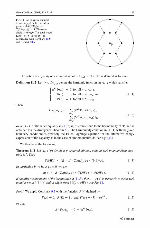
Fig. 10 An extrinsic minimal2-web W2(p) in the Euclideanplane with #(∂W2(p))=T(∂ W2(p)) = 8. The outercircle is ∂B2(p). The total lengthL(W2) of W2(p) is 16—inaccordance with Corollary 10.5and Remark 10.6
p
The notion of capacity of a minimal annulus Aρ,R of G in Nn is defined as follows.
Definition 11.2 Let � ∈ DAρ,R denote the harmonic function on Aρ,R which satisfies⎧⎪⎨
⎪⎩
G�(x) = 0 for all x ∈ Aρ,R,�(x) = 0 for all x ∈ ∂Wρ and
�(x) = 1 for all x ∈ ∂WR.
(11.1)
Then
Cap(Aρ,R) = ∑∂Wρ
〈∇G�, ν(∂Wρ) 〉G= ∑
∂WR
〈∇G�, ν(∂WR) 〉G. (11.2)
Remark 11.3 The latter equality in (11.2) is, of course, due to the harmonicity of �, and isobtained via the divergence Theorem 5.3. The harmonicity equation in (11.1) with the givenboundary conditions is precisely the Euler–Lagrange equation for the alternative energyexpression of the capacity as in the case of smooth manifolds, see e.g. [33].
We then have the following
Theorem 11.4 Let Aρ,R(p) denote a p-centered minimal annular web in an ambient man-ifold Nn. Then
T(∂Wρ) ≤ (R − ρ) · Cap(Aρ,R) ≤ T(∂WR). (11.3)
In particular, if we let ρ go to 0, we get
m(p) ≤ R · Cap(A0,R) ≤ T(∂WR) ≤ #(∂WR). (11.4)
If equality occurs in one of the inequalities in (11.3), thenAρ,R(p) is isometric to a star webannulus (with #(∂WR) radial edges from ∂Wρ to ∂WR), see Fig.11.
Proof We apply Corollary 9.3 with the function F(r) defined by
F(ρ) = 0, F (R) = 1 , and F ′(r) = (R − ρ)−1 , (11.5)
so that
GF(r)|x ≥ 0 = G�(x), (11.6)
123

30 Geom Dedicata (2008) 133:7–34
Fig. 11 The extrinsic minimalstar web annulus A1,2(p)=W∗
2 (p)−W∗1 (p) in the
Euclidean plane
p
where �(x) is the solution to Eq. 11.1. The difference F(r(x)) − �(x) is hence a subhar-monic function on Aρ,R , and since the difference vanishes at the boundary ∂Aρ,R , we getfrom the maximum principle, that
F(r(x)) ≤ �(x) for all x ∈ Aρ,R. (11.7)
In particular, along the in-boundary and out-boundary the derivatives must therefore satisfythe following inequalities
〈 ∇GF(r(x)), ν(∂Wρ) 〉G ≤ 〈∇G�(x), ν(∂Wρ) 〉G,〈 ∇GF(r(x)), ν(∂WR) 〉G ≥ 〈∇G�(x), ν(∂WR) 〉G. (11.8)
It follows that
Cap(Aρ,R) = ∑∂Wρ
〈 ∇G�, ν(∂Wρ) 〉G≥ ∑
∂Wρ
〈 ∇GF(r(x)), ν(∂Wρ) 〉G= F ′(ρ) · T(∂Wρ)
= (R − ρ)−1 T(∂Wρ),
(11.9)
and similarly
Cap(Aρ,R) ≤ (R − ρ)−1 T(∂WR). (11.10)
If equality occurs in (11.9) or in (11.10), then we have a corresponding equality in Eq. 11.8as well. The boundary version of the maximum principle, Proposition 3.7, then applies andgives F(r(x)) = �(x) for all x ∈ Aρ,R . In particular all the edges in Aρ,R(p) must bedirected radially away from p, and this proves the theorem. �Remark 11.5 Equalities in (11.3) do not imply that all of the R-web WR is star shaped—consider e.g. the minimal annulus A1,2(p) of the example W2(p) in Fig. 10.
Definition 11.6 (Cf. [33]) A given complete metric graphG is transient if there is a precom-pact open domain� inG, such that the Brownian motionXt starting from� does not returnto � with probability 1, i.e.:
Px{ω |Xt(ω) ∈ � for some t > 0} < 1, (11.11)
otherwise G is called recurrent.
123

Geom Dedicata (2008) 133:7–34 31
In view of Remark 3.5, and since G = (V ,E) = (G, g), considered as a length spacecontinuum, is roughly isometric to (V , d), considered as a combinatorial metric space withthe metric d induced from the length space metric g, we obtain: Transience of the RandomWalk on V with respect to d is equivalent to transience of the G-driven Brownian Motionon G with respect to g, see e.g. [48].
In the literature there are several conditions for transience of manifolds and combinatorialgraphs. For example, Lyons [42] obtains transience from the existence of a finite energy flowfield on the graph. This, in turn, is applied by Thomassen in [61] to show transience from theexistence of a rooted isoperimetric profile function whose reciprocal is square integrable onthe graph. The corresponding statements for manifolds are established in [43] by Lyons andSullivan and in [29] by Fernandez, respectively.
The following is but one other consequence, which expresses transience in terms of capac-ities. The relation between these two notions is much more general than stated here (see e.g.[33,43]), but we only need the following for Corollary 11.7 below.
Proposition B A given complete minimal web G in an Hadamard–Cartan manifold is tran-sient if for some (hence any) fixed ρ we have
limR→∞ Cap(Aρ,R) > 0, (11.12)
From Theorem 11.4 we then conclude
Corollary 11.7 Let G denote a complete minimal web in an Hadamard–Cartan manifold.Let p ∈ G and let WR denote the p-centered R-web of G. Then G is recurrent if
limR→∞
(R
T(∂WR)
)= ∞. (11.13)
The so-called type problem is concerned with the challenging problem of establishing suf-ficient (and necessary) global ‘structural’ conditions for a given metric graph to be transient.
Remark 11.8 As already alluded to in Subsect. 2.1, Scherk’s web is transient. This is shownin [48] via the finite energy flow criterion of [42].
It is to be expected that minimal webs in Hadamard–Cartan manifolds are in fact transientunder conditions which should be quite mild in comparison with the intrinsic isoperimetrictype conditions alluded to above. This expectation is mainly motivated by the fact that mini-mally immersed submanifolds (of sufficient dimension) in Hadamard–Cartan manifolds aretransient without any further conditions:
Theorem C([51]) Let Pm be a complete minimally immersed submanifold of an Hadam-ard–Cartan manifold Nn with sectional curvatures bounded from above by b ≤ 0. Then Pm
is transient if either (b < 0 and m ≥ 2) or (b = 0 and m ≥ 3).However, it is not yet clear how to mold a similar condition like this ‘dimensionality
assumption’, which in a corresponding setting would work for minimally immersed metricgraphs as well.
Acknowledgements The author would like to thank the referee for excellent questions, corrections, andcomments, which greatly improved the presentation of this work.
123
32 Geom Dedicata (2008) 133:7–34
References
1. Anand, C.K.: Harmonic morphisms of metric graphs, In Harmonic morphisms, harmonic maps, andrelated topics. In: Anand, C.K., Baird, P., Loubeau, E., Wood, J.C. (eds.) Research Notes in Mathematicsvol. 413, pp. 109–112. Chapman & Hall (1999)
2. Barta, J.: Sur la vibration fundamentale d’une membrane. C. R. Acad. Sci. 204, 472–473 (1937)3. Below, J.von : A characteristic equation associated to an eigenvalue problem on c2−networks. Linear
Algebra Appl. 71, 309–325 (1985)4. Below, J.von : Sturm-Liouville eigenvalue problems on networks. Math. Meth. Appl. Sci. 10,
383–395 (1988)5. Bridson, M.R., Haefliger, A.: Metric Spaces of Non-positive Curvature, Grundlehren der Mathemat-
ischen Wissenschaften [Fundamental Principles of Mathematical Sciences], vol. 319. Springer-Verlag,Berlin (1999)
6. Bobenko, A.I., Hoffmann, T., Springborn, B.A.: Minimal surfaces from circle patterns: geometry fromcombinatorics. Annals Math. 164(2), 231–264 (2006)
7. Bobenko, A.I., Pinkall, U.: Discrete isothermic surfaces. J. Reine Angew. Math. 475, 187–208 (1996)8. Burago, D., Burago, Y., Ivanov, S.: A Course in Metric Geometry, Graduate Studies in Mathematics,
vol. 33. American Mathematical Society (2001)9. Cattaneo, C.: The spectrum of the continuous Laplacian on a graph. Monatsh. Math. 124,
215–235 (1997)10. Chavel, I.: Eigenvalues in Riemannian Geometry. Academic Press (1984)11. Chavel, I.: Riemannian Geometry: A Modern Introduction, Cambridge Tracts in Mathematics, vol. 108.
Cambridge University Press (1993)12. Chavel, I.: Isoperimetric Inequalities, Cambridge Tracts in Mathematics, vol. 145. Cambridge University
Press (2001)13. Cheng, S.Y., Li, P., Yau, S.T.: Heat equations on minimal submanifolds and their applications. Am.
J. Math. 106, 1033–1065 (1984)14. Chung, F.R.K.: Spectral Graph Theory, CBMS Regional Conference Series in Mathematics, vol. 92.
American Mathematical Society (1997)15. Chung, F., Yau, S.T.: Eigenvalue inequalities for graphs and convex subgraphs. Comm. Anal.
Geom. 5, 575–623 (1997)16. Coulhon, T., Grigor’yan, A.: Random walks on graphs with regular volume growth. GAFA, Geom.
Funct. Anal. 8, 656–701 (1998)17. Courant, R., Friedrichs, K., Lewy, H.: Über die partiellen Differenzengleichungen der Mathematischen
Physik. Math. Ann. 100, 32–74 (1928)18. Cvetkovic, D.M., Doob, M., Sachs, H.: Spectra of Graphs, Theory and Application. Academic Press
(1980)19. Davies, E.B.: Spectral Theory and Differential Operators, Cambridge Studies in Advanced Mathematics,
vol. 42. Cambridge University Press (1995)20. Deza, M.M., Laurent, M.: Geometry of Cuts and Metrics, Algorithms and Combinatorics, vol. 15.
Springer-Verlag (1997)21. Dodziuk, J.: Finite difference approach to the Hodge theory of harmonic forms. Am. J. Math. 98,
79–104 (1976)22. Dodziuk, J.: Difference equations, isoperimetric inequality, and transience of certain random
walks. Trans. Am. Math. Soc. 284, 787–794 (1984)23. Dodziuk, J., Karp, L.: Spectral and function theory for combinatorial Laplacian. Contemp. Math. 73, 25–
40 (1988)24. Dodziuk, J., Kendall, W.S.: Combinatorial Laplacians and isoperimetric inequality. In: Elworthy, K.D.
(eds.) From Local Times to Global Geometry, Control and Physics, Pitman Research Notes Math. Ser.,vol. 150, pp. 68–74 (1986)
25. Dynkin, E.B.: Markov Processes. Springer Verlag (1965)26. Eckmann, B.: Harmonische Funktionen und Randwertaufgaben in eiem Komplex. Comment. Math.
Helv. 17, 240–255 (1945)27. Eells, J., Fuglede, B.: Harmonic Maps between Riemannian Polyhedra, Cambridge Tracts in
Mathematics, vol. 142. Cambridge University Press (2001)28. Exner, P., Post, O.: Convergence of spectra of graph-like thin manifolds. J. Geom. Phys. 54,
77–115 (2005)29. Fernandez, J.L.: On the existence of Green’s function in a Riemannian manifold. Proc. Am. Math.
Soc. 96, 284–286 (1986)
123

Geom Dedicata (2008) 133:7–34 33
30. Friedman, J.: Some geometric aspects of graphs and their eigenfunctions. Duke Math. J. 69,487–525 (1993)
31. Friedman, J., Tillich, J.-P.: Wave equations for graphs and the edge-based Laplacian. PacificJ. Math. 216, 229–266 (2004)
32. Fujiwara, K.: Eigenvalues of Laplacians on a closed Riemannian Manifold and its Nets. Proc. Am.Math. Soc. 123, 2585–2594 (1995)
33. Grigor’yan, A.: Analytic and geometric background of recurrence and non-explosion of the Brownianmotion on riemannian manifolds. Bull. (N.S.) Am. Math. Soc. 36, 135–249 (1999)
34. Hodge, W.V.D.: The Theory and Applications of Harmonic Integrals. Cambridge at the UniversityPress (1959)
35. Jorge, L.P., Koutroufiotis, D.: An estimate for the curvature of bounded submanifolds. Am.J. Math. 103, 711–725 (1981)
36. Kanai, M.: Rough isometries and combinatorial approximations of geometries of non-compactRiemannian manifolds. J. Math. Soc. Jpn. 37, 391–413 (1985)
37. Kanai, M.: Rough isometries and the parabolicity of Riemannian manifolds. J. Math. Soc. Jpn. 38, 227–238 (1986)
38. Kanai, M.: Analytic inequalities and rough isometries between non-compact Riemannian manifolds,Curvature and topology of Riemannian manifolds. In: Shiohama, K., Sakai, T., Sunada, T. (eds.) LectureNotes in Mathematics 1201, pp. 122–137. Springer, Berlin (1986)
39. Kuchment, P.: Quantum graphs. I. Some basic structures. Waves Random Media 14, 107–128 (2004)40. Kuchment, P.: Quantum graphs. II. Some spectral properties of quantum and combinatorial graphs.
J. Phys. A 14, 4887–4900 (2005)41. Lions, J.L.: Problèmes aux limites dans les équations aux dérivées partielles. Séminaire de Mathéma-
tiques Supérieures Montréal. Univ. Press (1962)42. Lyons, T.: A simple criterion for transience of a reversible Markov chain. Ann. Probab. 11,
393–402 (1983)43. Lyons, T., Sullivan, D.: Function theory, random paths, and covering spaces. J. Diff. Geom. 19,
229–323 (1984)44. Markvorsen, S.: On the heat kernel comparison theorems for minimal submanifolds. Proc. Am. Math.
Soc. 97, 479–482 (1986)45. Markvorsen, S.: A characteristic eigenfunction for minimal submanifolds. Math. Z. 202, 375–382 (1989)46. Markvorsen, S.: On the mean exit time from a minimal submanifold. J. Diff. Geom. 29, 1–8 (1989)47. Markvorsen, S., Min-Oo, M.: Global Riemannian Geometry: Curvature and Topology, Advanced
Courses in Mathematics. CRM Barcelona. Birkhäuser (2003)48. Markvorsen, S., McGuinness, S., Thomassen, C.: Transient random walks on graphs and metric spaces
with applications to hyperbolic surfaces. Proc. London Math. Soc. 64, 1–20 (1992)49. Markvorsen, S., Palmer, V.: Generalized isoperimetric inequalities for extrinsic balls in minimal
submanifolds. J. Reine Angew. Math. 551, 101–121 (2002)50. Markvorsen, S., Palmer, V.: On the isoperimetric rigidity of extrinsic minimal balls. J. Diff. Geom.
Appl. 18, 47–54 (2003)51. Markvorsen, S., Palmer, V.: Transience and capacity of minimal submanifolds. Geom. Funct.
Anal. 13(4), 915–933 (2003)52. Mohar, B., Thomassen, C.: Graphs on Surfaces. The Johns Hopkins University Press (2001)53. Nicaise, S.: Approche spectrale des problèmes de diffusion sur les réseaux. Lect. Notes Math. 1235, 120–
140 (1989)54. Ohno, Y., Urakawa, H.: On the first eigenvalue of the combinatorial Laplacian for a graph. Interdiscip.
Inform. Sci. 1, 33–46 (1994)55. Palmer, V.: Isoperimetric Inequalities for extrinsic balls in minimal submanifolds and their applica-
tions. J. London Math. Soc. 60(2), 607–616 (1999)56. Reed, M., Simon, B.: Methods of Modern Mathematical Physics. I. Functional Analysis. Academic
Press, New York (1980)57. Roth, J.P.: Le spectra du Laplacien sur un graphe. Lect. Notes Math. 1096, 521–538 (1984)58. Sakai, T.: Riemannian Geometry, Translations of Mathematical Monographs, vol. 149. American
Mathematical Society (1996)59. Soardi, P.M.: Potential Theory on Infinite Networks, Lecture Notes in Mathematics, vol. 1590.
Springer-Verlag (1999)60. Smilansky, U., Solomyak, M.: The quantum graph as a limit of a network of physical wires. Quantum
Graphs and Their Applications. Contemp. Math. (Am. Math. Soc.) 415, 283–291 (2006)61. Thomassen, C.: Isoperimetric inequalities and transient random walks on graphs. Ann. Probab. 20, 1592–
1600 (1992)
123
34 Geom Dedicata (2008) 133:7–34
62. Tsuruta, T.: Harmonic morphisms on weighted graphs. J. Math. Sci. Univ. Tokyo 7, 297–310 (2000)63. Urakawa, H.: A discrete analogue of the harmonic morphism, Harmonic morphisms, harmonic maps,
and related topics. In: Anand, C.K., Baird, P., Loubeau, E., Wood, J.C. (eds.) Research Notes inMathematics, vol. 413, pp. 97–108. Chapman & Hall (1999)
64. Urakawa, H.: The Dirichlet eigenvalue problem, the finite element method and graph theory. Contemp.Math. 348, 221–232 (2004)
65. West, D.B.: Introduction to Graph theory. Prentice Hall (1996)66. Woess, W.: Random walks on infinite graphs and groups, Cambridge Tracts in Mathematics, vol. 138.
Cambridge University Press (2000)
123