mimo communications: technology...
TRANSCRIPT

MIMO Communications:An Overview of Concepts and
Applications
Brett T. Walkenhorst, Ph.D.Founder and Chief Engineer
Creydos Researchhttp://www.creydos.com/
My Background
• Lucent Technologies: RF/DSP design of GSM and Tri-band base stations
• Georgia Tech: PhD in MIMO Communications, research in signal processing and comms
• NSI-MI Technologies: signal processing for advanced antenna measurement techniques
• Creydos Research: Consulting in signal processing and machine learning related to RF systems and sensors

Creydos Research
• R&D Consulting Firm founded in 2015
• Seeking new partnerships
• Interest in IoT: Transitioning to a world in which everything is connected requires careful planning and expert modeling
• Creydos offers expertise in EM propagation, wireless comm, RF systems, and system architecture
Outline
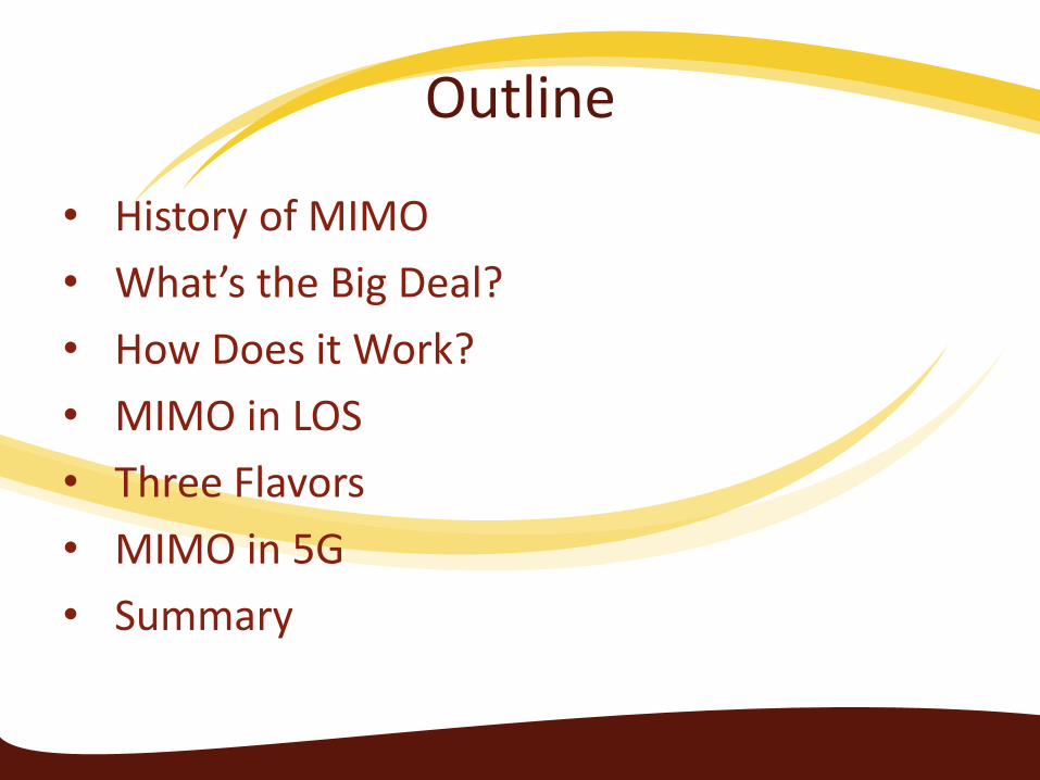
• History of MIMO
• What’s the Big Deal?
• How Does it Work?
• MIMO in LOS
• Three Flavors
• MIMO in 5G
• Summary

History of MIMO
• Invention attributed to multiple people/groups
– Clarity Wireless
– Bell Labs
– Iospan
• One of the most commonly cited paper is by Foschini and Gans in 1998 at Lucent, Bell Labs
– Information Theory focus
– Showed how MIMO created a new equation describing ‘capacity’ that far transcended our old understanding of wireless channel capacity

History of MIMO in Standards
• Wifi
– 802.11n, group created in 2003, final standard published in 2009
– First MIMO chipsets hit the market in 2004
• 4G
– WiMAX
• 802.16e
• 802.16m
– LTE
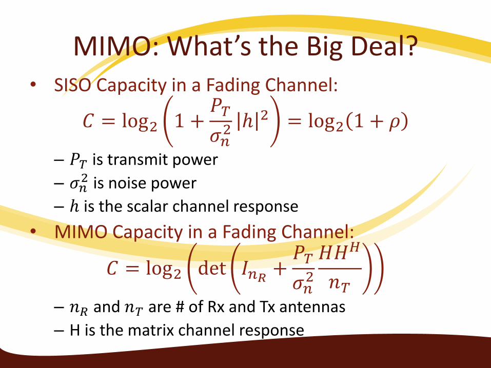
MIMO: What’s the Big Deal?• SISO Capacity in a Fading Channel:
𝐶 = log2 1 +𝑃𝑇
𝜎𝑛2 ℎ 2 = log2 1 + 𝜌
– 𝑃𝑇 is transmit power
– 𝜎𝑛2 is noise power
– ℎ is the scalar channel response
• MIMO Capacity in a Fading Channel:
𝐶 = log2 det 𝐼𝑛𝑅+
𝑃𝑇
𝜎𝑛2
𝐻𝐻𝐻
𝑛𝑇
– 𝑛𝑅 and 𝑛𝑇 are # of Rx and Tx antennas
– H is the matrix channel response
Beyond the Equations
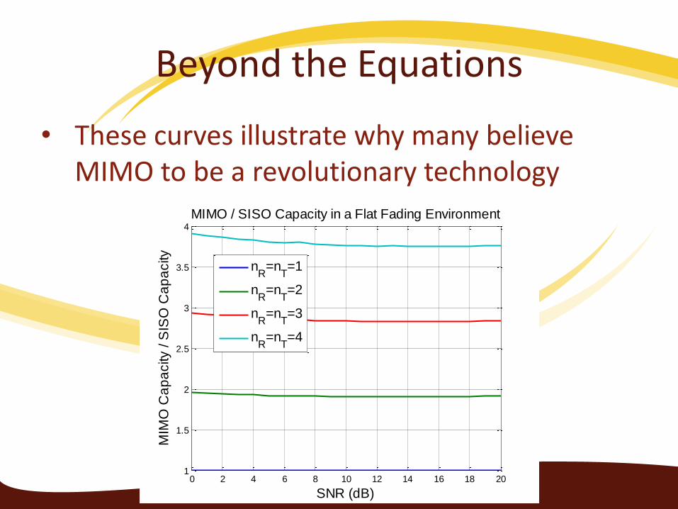
• These curves illustrate why many believe MIMO to be a revolutionary technology
0 2 4 6 8 10 12 14 16 18 200
5
10
15
20
25
SNR (dB)
Ca
pa
city (
bp
s/H
z)
Ergodic MIMO Capacity in a Flat Fading Environment
nR
=nT=1
nR
=nT=2
nR
=nT=3
nR
=nT=4
0 2 4 6 8 10 12 14 16 18 201
1.5
2
2.5
3
3.5
4
SNR (dB)
MIM
O C
ap
acity / S
ISO
Ca
pa
city
MIMO / SISO Capacity in a Flat Fading Environment
nR
=nT=1
nR
=nT=2
nR
=nT=3
nR
=nT=4

How Does it Work?
• SISO:– Signal model: 𝑦 = ℎ𝑥 + 𝑛
– Goal: Given 𝑦, find 𝑥
• MIMO:– Signal model: 𝑦 = 𝐻 𝑥 + 𝑛
– Goal: Given 𝑦, find 𝑥
• What used to be a simple scalar zero-forcing or MMSE detection problem is now a more complicated matrix/vector problem
MIMO
Receiver
MIMO
Transmitter
Channel
Matrix (H)
Wireless
Channel
RX
AntennasTX
Antennas
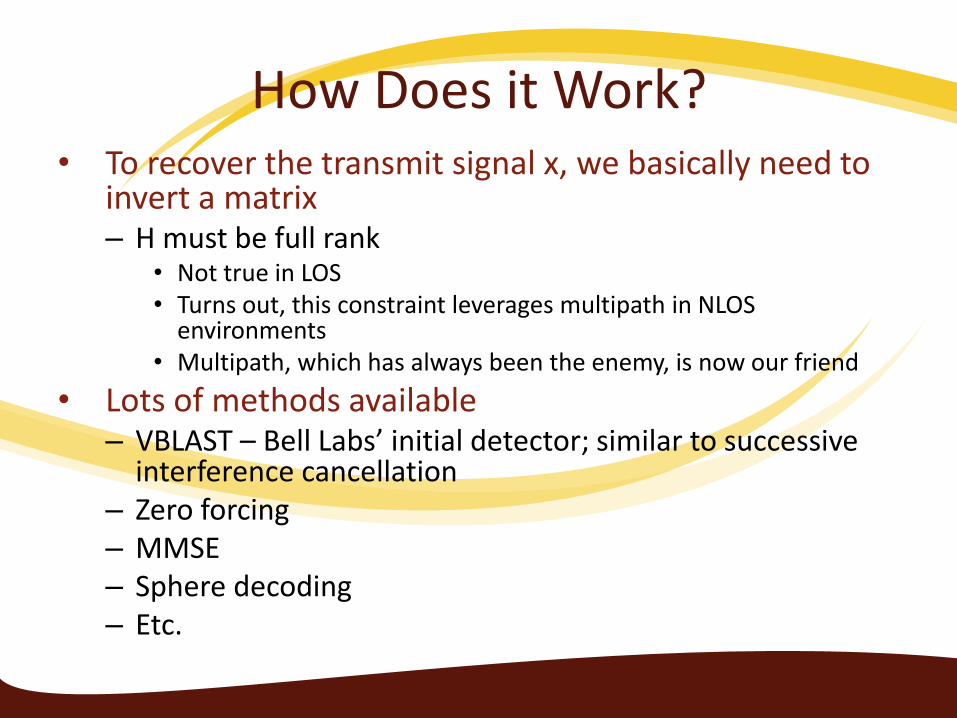
How Does it Work?• To recover the transmit signal x, we basically need to
invert a matrix– H must be full rank
• Not true in LOS• Turns out, this constraint leverages multipath in NLOS
environments• Multipath, which has always been the enemy, is now our friend
• Lots of methods available– VBLAST – Bell Labs’ initial detector; similar to successive
interference cancellation– Zero forcing– MMSE– Sphere decoding– Etc.
MIMO in LOS
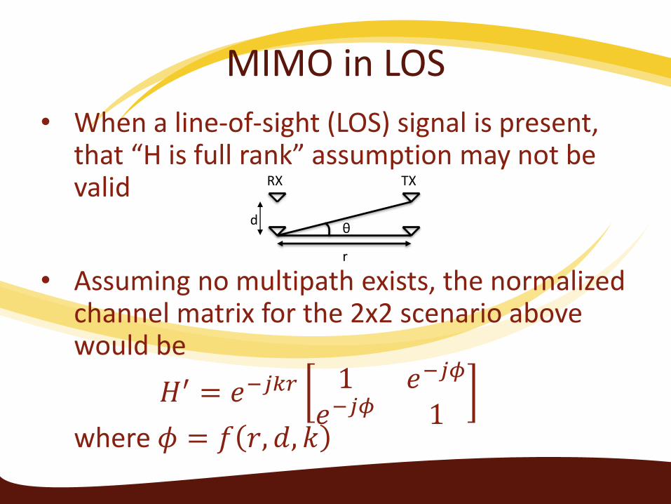
• When a line-of-sight (LOS) signal is present, that “H is full rank” assumption may not be valid
• Assuming no multipath exists, the normalized channel matrix for the 2x2 scenario above would be
𝐻′ = 𝑒−𝑗𝑘𝑟 1 𝑒−𝑗𝜙
𝑒−𝑗𝜙 1where 𝜙 = 𝑓 𝑟, 𝑑, 𝑘
d
r
θ
RX TX
LOS MIMO Capacity
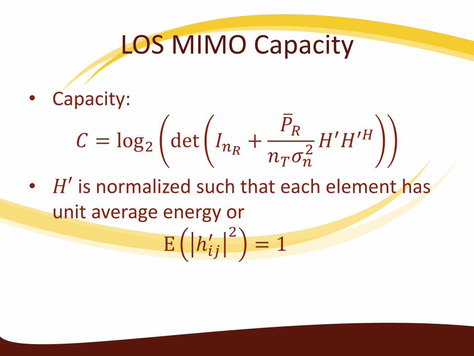
• Capacity:
𝐶 = log2 det 𝐼𝑛𝑅+
𝑃𝑅
𝑛𝑇𝜎𝑛2 𝐻′𝐻′𝐻
• 𝐻′ is normalized such that each element has unit average energy or
E ℎ𝑖𝑗′ 2
= 1
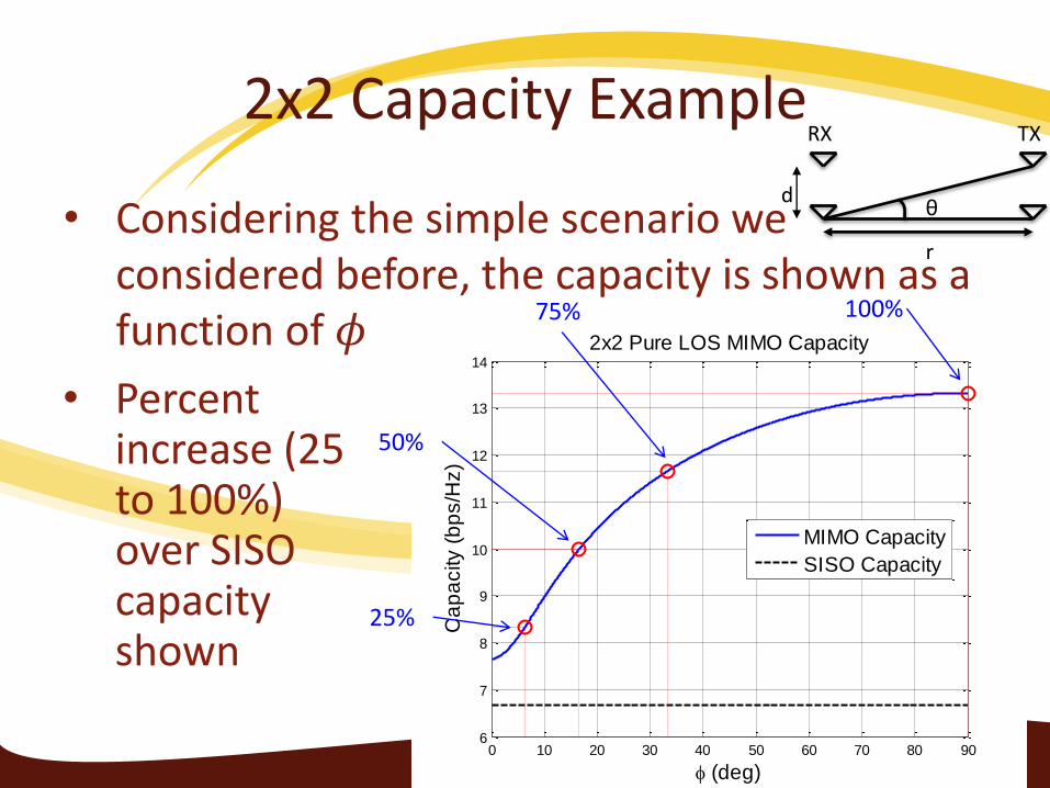
2x2 Capacity Example
• Considering the simple scenario we considered before, the capacity is shown as a function of 𝜙
d
r
θ
RX TX
0 10 20 30 40 50 60 70 80 906
7
8
9
10
11
12
13
14
(deg)
2x2 Pure LOS MIMO Capacity
Ca
pa
city (
bp
s/H
z)
MIMO Capacity
SISO Capacity
25%
50%
75% 100%
• Percent increase (25 to 100%) over SISO capacity shown
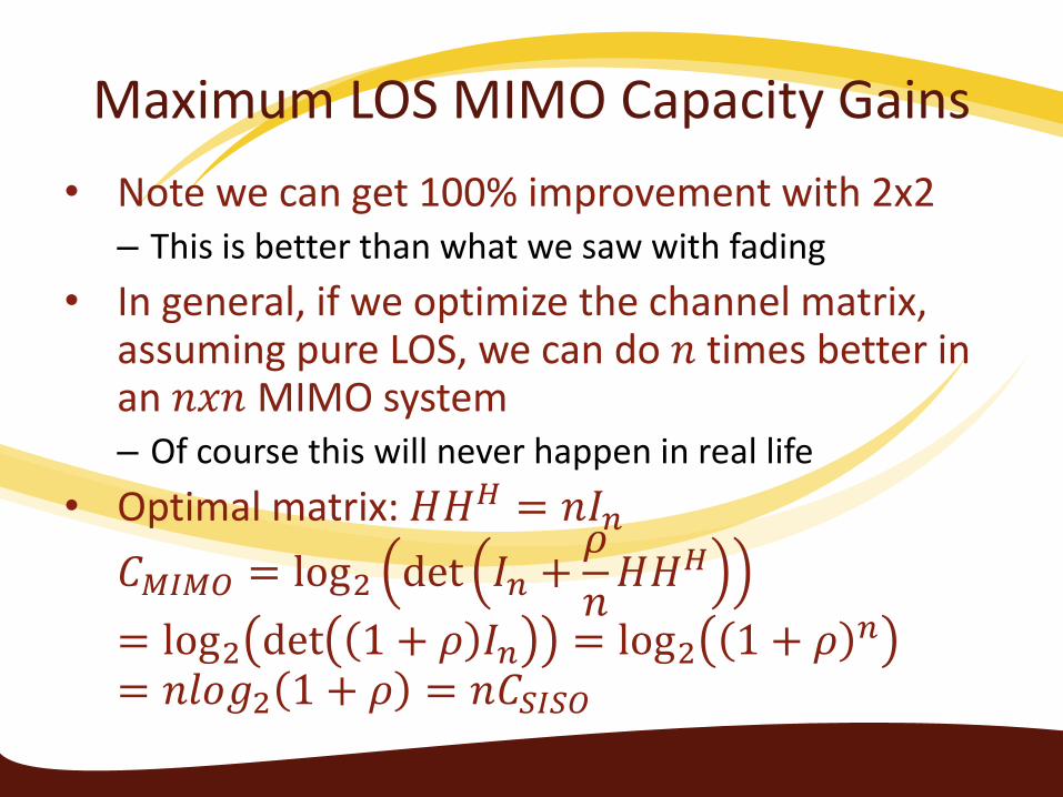
Maximum LOS MIMO Capacity Gains
• Note we can get 100% improvement with 2x2– This is better than what we saw with fading
• In general, if we optimize the channel matrix, assuming pure LOS, we can do 𝑛 times better in an 𝑛𝑥𝑛 MIMO system– Of course this will never happen in real life
• Optimal matrix: 𝐻𝐻𝐻 = 𝑛𝐼𝑛
𝐶𝑀𝐼𝑀𝑂 = log2 det 𝐼𝑛 +𝜌
𝑛𝐻𝐻𝐻
= log2 det 1 + 𝜌 𝐼𝑛 = log2 1 + 𝜌 𝑛
= 𝑛𝑙𝑜𝑔2 1 + 𝜌 = 𝑛𝐶𝑆𝐼𝑆𝑂
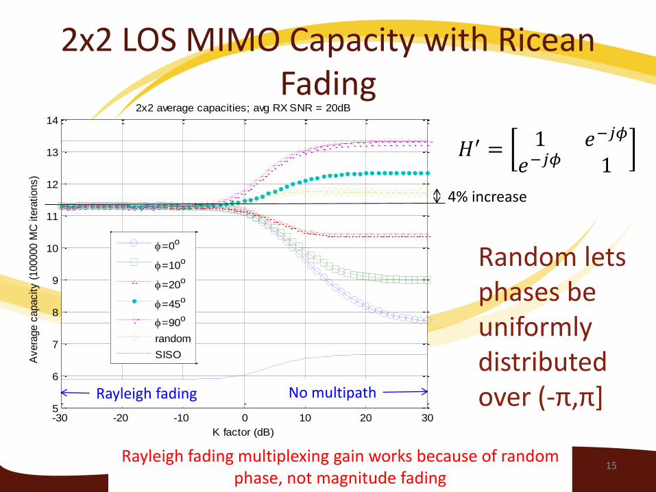
2x2 LOS MIMO Capacity with RiceanFading
Random lets phases be uniformly distributed over (-π,π]
-30 -20 -10 0 10 20 305
6
7
8
9
10
11
12
13
14
K factor (dB)
Avera
ge c
apacity (
100000 M
C ite
rations)
2x2 average capacities; avg RX SNR = 20dB
=0o
=10o
=20o
=45o
=90o
random
SISO
15Rayleigh fading multiplexing gain works because of random
phase, not magnitude fading
4% increase
Rayleigh fading No multipath
𝐻′ = 1 𝑒−𝑗𝜙
𝑒−𝑗𝜙 1
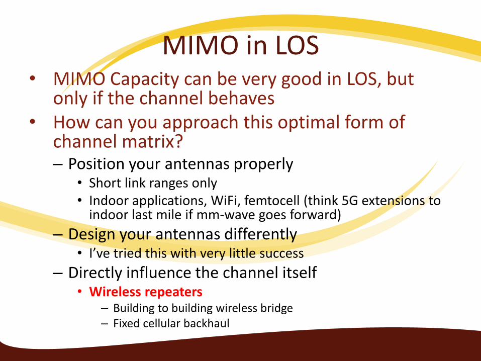
MIMO in LOS• MIMO Capacity can be very good in LOS, but
only if the channel behaves• How can you approach this optimal form of
channel matrix?– Position your antennas properly
• Short link ranges only• Indoor applications, WiFi, femtocell (think 5G extensions to
indoor last mile if mm-wave goes forward)
– Design your antennas differently• I’ve tried this with very little success
– Directly influence the channel itself• Wireless repeaters
– Building to building wireless bridge– Fixed cellular backhaul
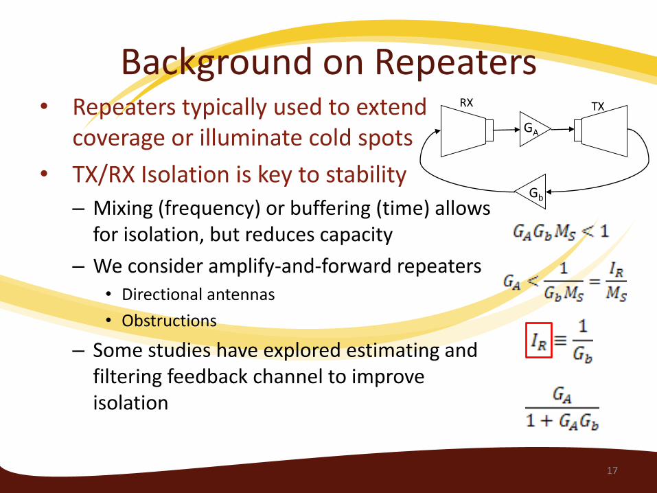
Background on Repeaters• Repeaters typically used to extend
coverage or illuminate cold spots
• TX/RX Isolation is key to stability
– Mixing (frequency) or buffering (time) allows for isolation, but reduces capacity
– We consider amplify-and-forward repeaters• Directional antennas
• Obstructions
– Some studies have explored estimating and filtering feedback channel to improve isolation
GA
RX TX
Gb
17
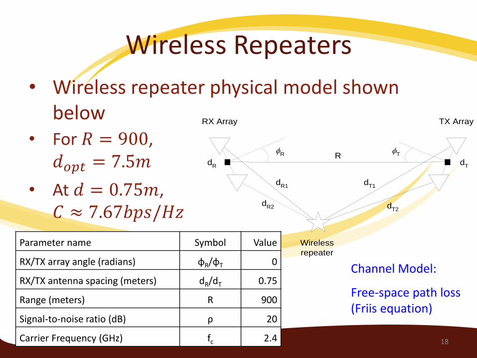
Wireless Repeaters
• Wireless repeater physical model shown below
Channel Model:
Free-space path loss (Friis equation)
18
R
R
T. .RX Array TX Array
Wireless
repeater
dR1
dR
dT
dR2
dT1
dT2
Parameter name Symbol Value
RX/TX array angle (radians) φR/φT 0
RX/TX antenna spacing (meters) dR/dT 0.75
Range (meters) R 900
Signal-to-noise ratio (dB) ρ 20
Carrier Frequency (GHz) fc 2.4
• For 𝑅 = 900, 𝑑𝑜𝑝𝑡 = 7.5𝑚
• At 𝑑 = 0.75𝑚, 𝐶 ≈ 7.67𝑏𝑝𝑠/𝐻𝑧

x position (m)
y p
ositio
n (
m)
Capacity (bps/Hz)
0 200 400 600 800 1000
-80
-60
-40
-20
0
20
40
60
80
2
4
6
8
10
12
14
Capacity with Repeater
• Capacity as a function of repeater position
• Distinct regions of optimal placement
• Notice noise amplification effects
RX TX
19
Let’s look at a cross-section of these 2 plots when x = 450m

x position (m)
y p
ositio
n (
m)
Capacity (bps/Hz)
0 200 400 600 800 1000
-80
-60
-40
-20
0
20
40
60
80
2
4
6
8
10
12
14
x position (m)
y p
ositio
n (
m)
1% Outage Capacity (bps/Hz)
0 200 400 600 800 1000
-80
-60
-40
-20
0
20
40
60
802
4
6
8
10
12
Capacity with Repeater
• Capacity as a function of repeater position
• Distinct regions of optimal placement
• Notice noise amplification effects
RX TXWith multipath
K = 10dB
20
Let’s look at a cross-section of these 2 plots when x = 450m

-80 -60 -40 -20 0 20 40 60 800
2
4
6
8
10
12
14
16
y position (m)
1%
Outa
ge C
apacity (
bps/H
z)
2 x 2 Capacity; dr = 0.75m; dt = 0.75m; SNR = 20dB
Repeater
Ideal Repeater
optimal repeater
optimal 2x2
baseline
worst case
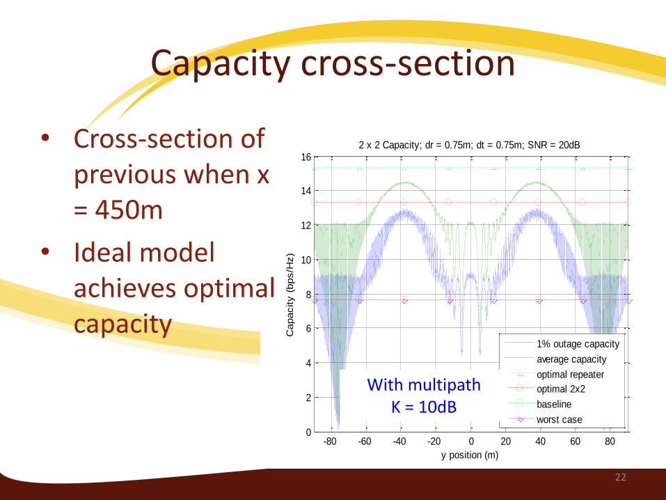
Capacity cross-section
• Cross-section of previous when x = 450m
• Ideal model achieves optimal capacity
21
-80 -60 -40 -20 0 20 40 60 800
2
4
6
8
10
12
14
16
y position (m)
1%
Outa
ge C
apacity (
bps/H
z)
2 x 2 Capacity; dr = 0.75m; dt = 0.75m; SNR = 20dB
Repeater
Ideal Repeater
optimal repeater
optimal 2x2
baseline
worst case
-80 -60 -40 -20 0 20 40 60 800
2
4
6
8
10
12
14
16
y position (m)
Capacity (
bps/H
z)
2 x 2 Capacity; dr = 0.75m; dt = 0.75m; SNR = 20dB
1% outage capacity
average capacity
optimal repeater
optimal 2x2
baseline
worst case
Capacity cross-section
• Cross-section of previous when x = 450m
• Ideal model achieves optimal capacity
With multipathK = 10dB
22

Positioning metric (cont’d)
23
x position (m)y p
ositio
n (
m)
(nR-|y
RX|)(n
T-|y
TX|)
0 200 400 600 800 1000
-80
-60
-40
-20
0
20
40
60
80
0.5
1
1.5
2
2.5
3
3.5
x position (m)
y p
ositio
n (
m)
det(HHH)
0 200 400 600 800 1000
-80
-60
-40
-20
0
20
40
60
80
2
4
6
8
10
12
14
Null-space positioning metric
Determinant metric det(HHH)
• A simple metric and implementation method exists without relying on a detailed channel model and analysis like I presented in prior slides
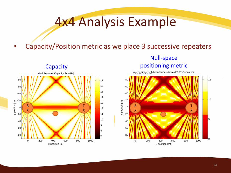
4x4 Analysis Example
• Capacity/Position metric as we place 3 successive repeaters
x position (m)
y p
ositio
n (
m)
Ideal Repeater Capacity (bps/Hz)
0 200 400 600 800 1000
-80
-60
-40
-20
0
20
40
60
807
8
9
10
11
12
13
14
15
16
17
x position (m)
y p
ositio
n (
m)
(nR-|y
RX|)(n
T-|y
TX|) beamformers toward TX/RX/repeaters
0 200 400 600 800 1000
-80
-60
-40
-20
0
20
40
60
80
0
5
10
15
RX
TX
RX
TX
Capacity
Null-space positioning metric
24

4x4 Analysis Example
• Capacity/Position metric as we place 3 successive repeaters
x position (m)
y p
ositio
n (
m)
Ideal Repeater Capacity (bps/Hz)
0 200 400 600 800 1000
-80
-60
-40
-20
0
20
40
60
807
8
9
10
11
12
13
14
15
16
17
x position (m)
y p
ositio
n (
m)
(nR-|y
RX|)(n
T-|y
TX|) beamformers toward TX/RX/repeaters
0 200 400 600 800 1000
-80
-60
-40
-20
0
20
40
60
80
0
5
10
15
x position (m)
y p
ositio
n (
m)
Ideal Repeater Capacity (bps/Hz)
0 200 400 600 800 1000
-80
-60
-40
-20
0
20
40
60
80
14
16
18
20
22
24
26
x position (m)
y p
ositio
n (
m)
(nR-|y
RX|)(n
T-|y
TX|) beamformers toward TX/RX/repeaters
0 200 400 600 800 1000
-80
-60
-40
-20
0
20
40
60
80
50
100
150
200
RX
TX
RX
TX
Capacity
Null-space positioning metric
25

4x4 Analysis Example
• Capacity/Position metric as we place 3 successive repeaters
x position (m)
y p
ositio
n (
m)
Ideal Repeater Capacity (bps/Hz)
0 200 400 600 800 1000
-80
-60
-40
-20
0
20
40
60
807
8
9
10
11
12
13
14
15
16
17
x position (m)
y p
ositio
n (
m)
(nR-|y
RX|)(n
T-|y
TX|) beamformers toward TX/RX/repeaters
0 200 400 600 800 1000
-80
-60
-40
-20
0
20
40
60
80
0
5
10
15
x position (m)
y p
ositio
n (
m)
Ideal Repeater Capacity (bps/Hz)
0 200 400 600 800 1000
-80
-60
-40
-20
0
20
40
60
80
14
16
18
20
22
24
26
x position (m)
y p
ositio
n (
m)
(nR-|y
RX|)(n
T-|y
TX|) beamformers toward TX/RX/repeaters
0 200 400 600 800 1000
-80
-60
-40
-20
0
20
40
60
80
50
100
150
200
x position (m)
y p
ositio
n (
m)
Ideal Repeater Capacity (bps/Hz)
0 200 400 600 800 1000
-80
-60
-40
-20
0
20
40
60
80
22
24
26
28
30
32
34
x position (m)
y p
ositio
n (
m)
(nR-|y
RX|)(n
T-|y
TX|) beamformers toward TX/RX/repeaters
0 200 400 600 800 1000
-80
-60
-40
-20
0
20
40
60
80
0
500
1000
1500
2000
2500
3000
3500
RX
TX
RX
TX
Capacity
Null-space positioning metric
26
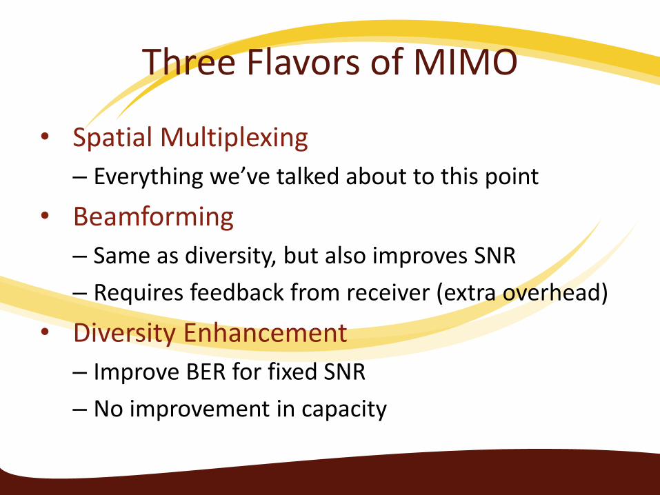
Three Flavors of MIMO
• Spatial Multiplexing
– Everything we’ve talked about to this point
• Beamforming
– Same as diversity, but also improves SNR
– Requires feedback from receiver (extra overhead)
• Diversity Enhancement
– Improve BER for fixed SNR
– No improvement in capacity
Beamforming
• By estimating channel state information (CSI) or the channel matrix H, we can form beams to maximize the received SNR– We can form a single beam from all 𝑛𝑇 transmit
antennas and another single beam from all 𝑛𝑅 receive antennas
– We can also form multiple beams and send multiple data streams
• These ‘beams’ don’t make much physical sense in the conventional beamforming paradigm– Sometimes called ‘eigenbeams’
– Use eigenvectors of 𝐻𝐻𝐻
Image from: http://www.teletopix.org/4g-lte/beamforming-in-lte/
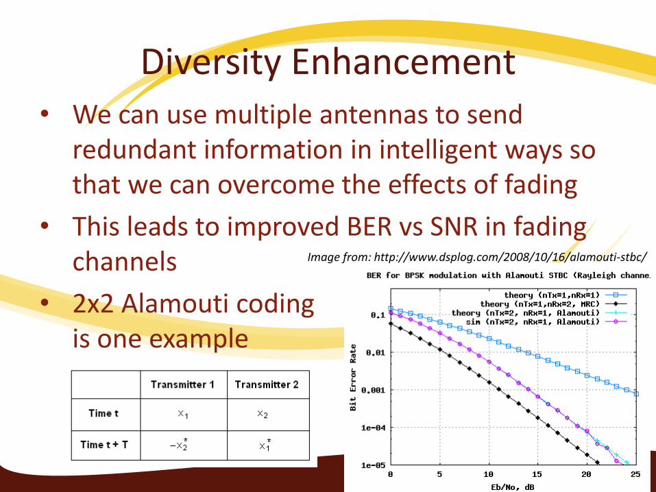
Diversity Enhancement• We can use multiple antennas to send
redundant information in intelligent ways so that we can overcome the effects of fading
• This leads to improved BER vs SNR in fading channels
• 2x2 Alamouti codingis one example
Image from: http://www.dsplog.com/2008/10/16/alamouti-stbc/
What Flavor to Pick?
• Depends on your configuration
• Recommended Approach: apply degrees of freedom to spatial multiplexing to the extent possible and apply remaining DoFs to either diversity enhancement or beamforming
• Three flavors of ice cream is better than one … right?
Applications of MIMO
• WiFi
• Backhaul
• Cellular– MIMO has been an important element in achieving
significant improvement in 4G
– A new flavor of MIMO looks like it may be an important contributor in 5G
• Any wireless link where we can afford extra antennas and want improved throughput and/or link reliability

MIMO in 5G
• 5G is looking at something called ‘massive MIMO’
• Antenna arrays on the order of 100 elements
• This is really multi-user MIMO using primarily beamforming with potential for multiplexing gain
• Coupled with mm-wave carrier frequencies, massive MIMO offers some advantages
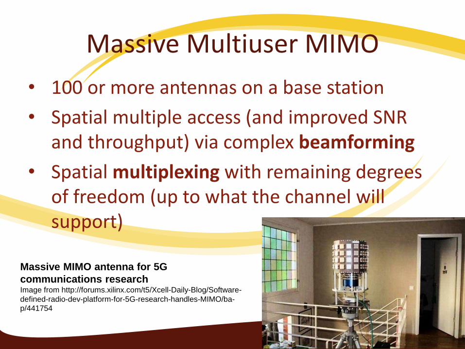
Massive Multiuser MIMO
• 100 or more antennas on a base station
• Spatial multiple access (and improved SNR and throughput) via complex beamforming
• Spatial multiplexing with remaining degrees of freedom (up to what the channel will support)
34
Massive MIMO antenna for 5G
communications researchImage from http://forums.xilinx.com/t5/Xcell-Daily-Blog/Software-
defined-radio-dev-platform-for-5G-research-handles-MIMO/ba-p/441754
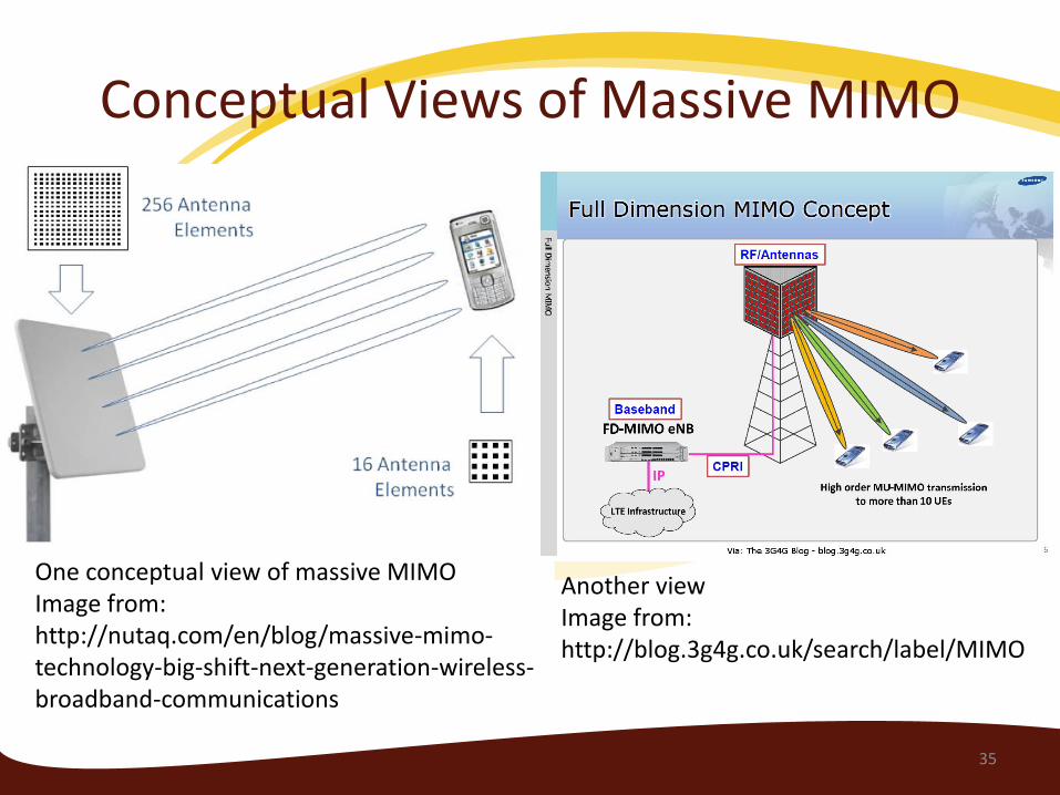
Conceptual Views of Massive MIMO
35
One conceptual view of massive MIMOImage from: http://nutaq.com/en/blog/massive-mimo-technology-big-shift-next-generation-wireless-broadband-communications
Another viewImage from: http://blog.3g4g.co.uk/search/label/MIMO

Millimeter-wave• Seeking to drastically improve data rates,
spectrum is the biggest crunch
• Options being discussed
– Confluence of fiber and wireless
– Smaller cell sizes with greater frequency reuse in dense urban environments
– Millimeter-wave
• Lots of options for carrier frequency
• Large instantaneous bandwidth
36
Image from: J. Laskar, et al, “The next wireless wave is a millimeter-wave,” Microwave Journal, Aug 2007.

Challenges of mmWave• Propagation
– Free space spreading loss is a function of wavelength
• For fixed antenna gains, we get very large spreading losses
– Omnidirectional links
– Short range
• For fixed antennas sizes, we get very directional antennas
– We can close our links better, but we need a way to handshake and then closely track CSI so we can point our beams
– Shadowing: physical structures start to look opaque at these wavelengths
• This can work with very small cells
• Indoor augmentation of terrestrial outdoor network
37
Massive MIMO and mmWave
• Combination of massive MIMO and millimeter-wave– Presents interesting challenges similar to search/track
radar
– If we insist on maintaining reasonable outdoor link ranges
• Higher atmospheric attenuation leads to smaller range– Ok in some environments
– Especially if networks move toward smaller cells
38
Summary
• MIMO
– Approaching 20 years old
– Requires multiple antennas at Tx and Rx
• Antennas can be orthogonal polarizations
– Advantages
• Improve throughput
• Improve reliability
