arX

iv:1

105.

4999

v3 [

cs.IT

] 15

Feb

201

3

MIMO Broadcasting for Simultaneous Wireless

Information and Power TransferRui Zhang and Chin Keong Ho

Abstract

Wireless power transfer (WPT) is a promising new solution toprovide convenient and perpetual energy

supplies to wireless networks. In practice, WPT is implementable by various technologies such as inductive

coupling, magnetic resonate coupling, and electromagnetic (EM) radiation, for short-/mid-/long-range applications,

respectively. In this paper, we consider the EM or radio signal enabled WPT in particular. Since radio signals

can carry energy as well as information at the same time, a unified study onsimultaneous wireless information

and power transfer(SWIPT) is pursued. Specifically, this paper studies a multiple-input multiple-output (MIMO)

wireless broadcast system consisting of three nodes, whereone receiver harvests energy and another receiver decodes

information separately from the signals sent by a common transmitter, and all the transmitter and receivers may

be equipped with multiple antennas. Two scenarios are examined, in which the information receiver and energy

receiver areseparatedand see different MIMO channels from the transmitter, orco-locatedand see the identical

MIMO channel from the transmitter. For the case of separatedreceivers, we derive the optimal transmission strategy

to achieve different tradeoffs for maximal information rate versus energy transfer, which are characterized by the

boundary of a so-calledrate-energy(R-E) region. For the case of co-located receivers, we show an outer bound for

the achievable R-E region due to the potential limitation that practical energy harvesting receivers are not yet able to

decode information directly. Under this constraint, we investigate two practical designs for the co-located receiver

case, namelytime switchingand power splitting, and characterize their achievable R-E regions in comparison to

the outer bound.

Index Terms

MIMO system, broadcast channel, precoding, wireless power, simultaneous wireless information and power

transfer (SWIPT), rate-energy tradeoff, energy harvesting.

I. INTRODUCTION

Energy-constrained wireless networks, such as sensor networks, are typically powered by batteries that have

limited operation time. Although replacing or recharging the batteries can prolong the lifetime of the network to

a certain extent, it usually incurs high costs and is inconvenient, hazardous (say, in toxic environments), or even

impossible (e.g., for sensors embedded in building structures or inside human bodies). A more convenient, safer,

as well as “greener” alternative is thus to harvest energy from the environment, which virtually provides perpetual

This paper has been presented in part at IEEE Global Communications Conference (Globecom), December 5-9, 2011, Houston, USA.

R. Zhang is with the Department of Electrical and Computer Engineering, National University of Singapore (e-mail:elezhang@nus.edu.sg).

He is also with the Institute for Infocomm Research, A*STAR,Singapore.

C. K. Ho is with the Institute for Infocomm Research, A*STAR,Singapore (e-mail:hock@i2r.a-star.edu.sg).

2

energy supplies to wireless devices. In addition to other commonly used energy sources such as solar and wind,

ambient radio-frequency (RF) signals can be a viable new source for energy scavenging. It is worth noting that

RF-based energy harvesting is typically suitable for low-power applications (e.g., sensor networks), but also can

be applied for scenarios with more substantial power consumptions if dedicated wireless power transmission is

implemented.1

On the other hand, since RF signals that carry energy can at the same time be used as a vehicle for transporting

information,simultaneous wireless information and power transfer(SWIPT) becomes an interesting new area of

research that attracts increasing attention. Although a unified study on this topic is still in the infancy stage, there

have been notable results reported in the literature [1], [2]. In [1], Varshney first proposed acapacity-energyfunction

to characterize the fundamental tradeoffs in simultaneousinformation and energy transfer. For the single-antenna

or SISO (single-input single-output) AWGN (additive whiteGaussian noise) channel with amplitude-constrained

inputs, it was shown in [1] that there exist nontrivial tradeoffs in maximizing information rate versus (vs.) power

transfer by optimizing the input distribution. However, ifthe average transmit-power constraint is considered instead,

the above two goals can be shown to be aligned for the SISO AWGNchannel with Gaussian input signals, and thus

there is no nontrivial tradeoff. In [2], Grover and Sahai extended [1] to frequency-selective single-antenna AWGN

channels with the average power constraint, by showing thata non-trivial tradeoff exists in frequency-domain

power allocation for maximal information vs. energy transfer.

As a matter of fact,wireless power transfer(WPT) or in shortwireless power, which generally refers to the

transmissions of electrical energy from a power source to one or more electrical loads without any interconnecting

wires, has been investigated and implemented with a long history. Generally speaking, WPT is carried out using

either the “near-field” electromagnetic (EM) induction (e.g., inductive coupling, capacitive coupling) for short-

distance (say, less than a meter) applications such as passive radio-frequency identification (RFID) [3], or the

“far-field” EM radiation in the form of microwaves or lasers for long-range (up to a few kilometers) applications

such as the transmissions of energy from orbiting solar power satellites to Earth or spacecrafts [4]. However, prior

research on EM radiation based WPT, in particular over the RFband, has been pursued independently from that

on wireless information transfer (WIT) or radio communication. This is non-surprising since these two lines of

work in general have very different research goals: WIT is tomaximize theinformation transmission capacityof

wireless channels subject to channel impairments such as the fading and receiver noise, while WPT is to maximize

the energy transmission efficiency(defined as the ratio of the energy harvested and stored at thereceiver to that

consumed by the transmitter) over a wireless medium. Nevertheless, it is worth noting that the design objectives

1Interested readers may visit the company website of Powercast at http://www.powercastco.com/ for more information onrecent

applications of dedicated RF-based power transfer.

3

Energy Flow

Information Flow Information Flow

Access Point

User Terminals

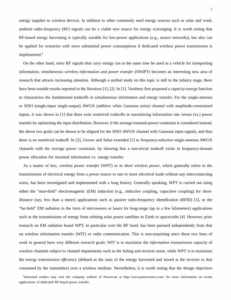
Fig. 1. A wireless network with dual information and energy transfer.

for WPT and WIT systems can be aligned, since given a transmitter energy budget, maximizing the signal power

received (for WPT) is also beneficial in maximizing the channel capacity (for WIT) against the receiver noise.

Hence, in this paper we attempt to pursue a unified study on WITand WPT for emerging wireless applications

with such a dual usage. An example of such wireless dual networks is envisaged in Fig. 1, where a fixed access

point (AP) coordinates the two-way communications to/froma set of distributed user terminals (UTs). However,

unlike the conventional wireless network in which both the AP and UTs draw energy from constant power supplies

(by e.g. connecting to the grid or a battery), in our model, only the AP is assumed to have a constant power source,

while all UTs need to replenish energy from the received signals sent by the AP via the far-field RF-based WPT.

Consequently, the AP needs to coordinate the wireless information and energy transfer to UTs in the downlink,

in addition to the information transfer from UTs in the uplink. Wireless networks with such a dual information

and power transfer feature have not yet been studied in the literature to our best knowledge, although some of

their interesting applications have already appeared in, e.g., the body sensor networks [5] with the out-body local

processing units (LPUs) powered by battery communicating and at the same time sending wireless power to in-body

sensors that have no embedded power supplies. However, how to characterize the fundamental information-energy

transmission tradeoff in such dual networks is still an openproblem.

In this paper, we focus our study on the downlink case with simultaneous WIT and WPT from the AP to UTs.

In the generic system model depicted in Fig. 1, each UT can in general harvest energy and decode information

at the same time (by e.g. applying the power splitting schemeintroduced later in this paper). However, from

an implementation viewpoint, one particular design whereby each UT operates as either an information receiver

or an energy receiver at any given time may be desirable, which is referred to astime switching. This scheme

is practically appealing since state-of-the-art wirelessinformation and energy receivers are typically designed to

operate separately with very different power sensitivities (e.g.,−50dBm for information receivers vs.−10dBm

for energy receivers). As a result, if time switching is employed at each UT jointly with the “near-far” based

4

transmission scheduling at the AP, i.e., UTs that are close to the AP and thus receive high power from the AP are

scheduled for WET, whereas those that are more distant from the AP and thus receive lower power are scheduled

for WIT, then SWIPT systems can be efficiently implemented with existing information and energy receivers and

the additional time-switching device at each receiver.

For an initial study on SWIPT, this paper considers the simplified scenarios with only one or two active UTs

in the network at any given time. For the case of two UTs, we assume time switching, i.e., the two UTs take

turns to receive energy or (independent) information from the AP over different time blocks. As a result, when

one UT receives information from the AP, the other UT can opportunistically harvest energy from the same signal

broadcast by the AP, and vice versa. Hence, at each block, oneUT operates as an information decoding (ID)

receiver, and the other UT as an energy harvesting (EH) receiver. We thus refer to this case asseparated EH and

ID receivers. On the other hand, for the case with only one single UT to be active at one time (while all other UTs

are assumed to be in the off/sleep mode), the active UT needs to harvest energy as well as decode information from

the same signal sent by the AP, i.e., the same set of receivingantennas are shared by both EH and ID receivers

residing in the same UT. Thus, this case is referred to asco-located EH and ID receivers. Surprisingly, as we

will show later in this paper, the optimal information-energy tradeoff for the case of co-located receivers is more

challenging to characterize than that for the case of separated receivers, due to a potential limitation that practical

EH receiver circuits are not yet able to decode the information directly and vice versa. Note that similar to the

case of separated receives, time switching can also be applied in the case of co-located receivers to orthogonalize

the information and energy transmissions at each receivingantenna; however, this scheme is in general suboptimal

for the achievable rate-energy tradeoffs in the case of co-located receivers, as will be shown later in this paper.

Some further assumptions are made in this paper for the purpose of exposition. Firstly, this paper considers a

quasi-static fading environment where the wireless channel between the AP and each UT is assumed to be constant

over a sufficiently long period of time during which the number of transmitted symbols can be approximately

regarded as being infinitely large. Under this assumption, we further assume that it is feasible for each UT to

estimate the downlink channel from the AP and then send it back to the AP via the uplink, since the time overhead

for such channel estimation and feedback is a negligible portion of the total transmission time due to quasi-static

fading. We will address the more general case of fading channels with imperfect/partial channel knowledge at the

transmitter in our future work. Secondly, we assume that thesystem under our study typically operates at the high

signal-to-noise ratio (SNR) regime for the ID receiver in the case of co-located receivers. This is to be compatible

with the high-power operating requirement for the EH receiver of practical interest as previously mentioned. Thirdly,

without loss of generality, we assume a multi-antenna or MIMO (multiple-input multiple-output) system, in which

5

MM

Energy Receiver

M

Transmitter

MM

Information Receiver

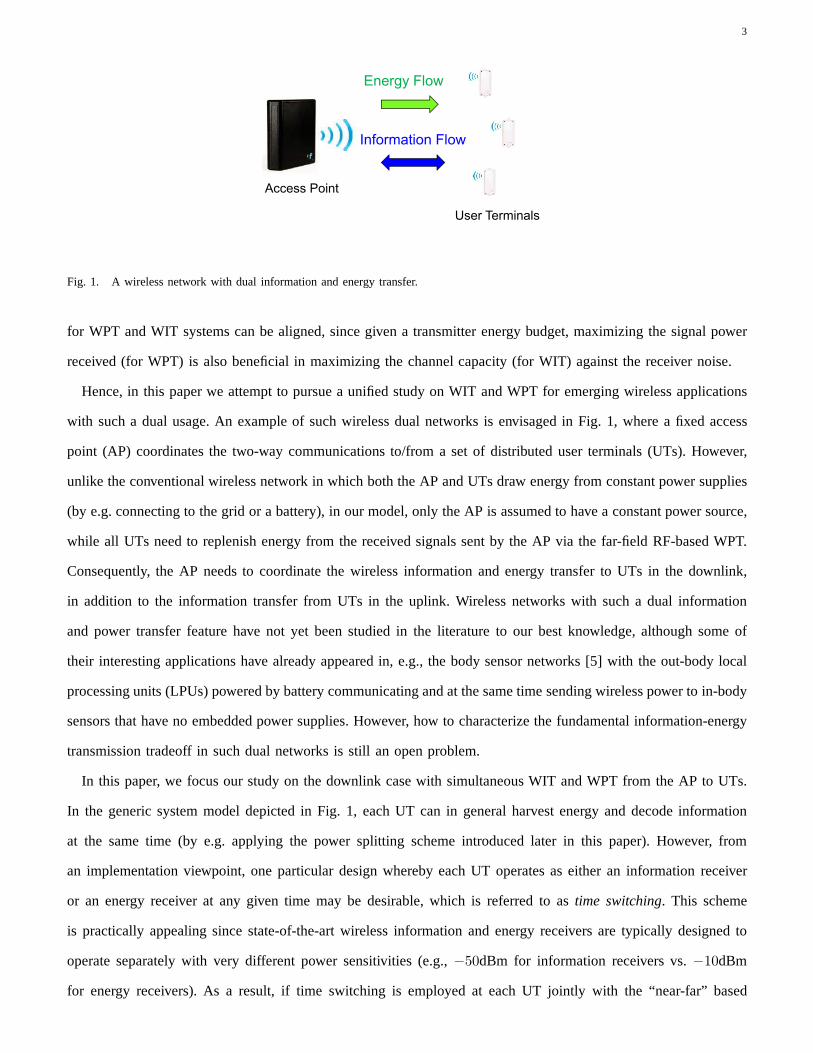
Fig. 2. A MIMO broadcast system for simultaneous wireless information and power transfer.

the AP is equipped with multiple antennas, and each UT is equipped with one or more antennas, for enabling

both the high-performance wireless energy and informationtransmissions (as it is well known that for WIT only,

MIMO systems can achieve folded array/capacity gains over SISO systems by spatial beamforming/multiplexing

[6]).

Under the above assumptions, a three-node MIMO broadcast system is considered in this paper, as shown in

Fig. 2, wherein the EH and ID receivers harvest energy and decode information separately from the signal sent

by a common transmitter. Note that this system model refers to the case of separated EH and ID receivers in

general, but includes the co-located receivers as a specialcase when the MIMO channels from the transmitter to

both receivers become identical. Assuming this model, the main results of this paper are summarized as follows:

• For the case of separated EH and ID receivers, we design the optimal transmission strategy to achieve different

tradeoffs between maximal information rate vs. energy transfer, which are characterized by the boundary

of a so-calledrate-energy(R-E) region. We derive a semi-closed-form expression for the optimal transmit

covariance matrix (for the joint precoding and power allocation) to achieve different rate-energy pairs on the

boundary of the R-E region. Note that the R-E region is a multiuser extension of the single-user capacity-

energy function in [1]. Also note that the multi-antenna broadcast channel (BC) has been investigated in e.g.

[7]–[12] for information transfer solely by unicasting or multicasting. However, MIMO-BC for SWIPT as

considered in this paper is new and has not yet been studied byany prior work.

• For the case of co-located EH and ID receivers, we show that the proposed solution for the case of separated

receivers is also applicable with the identical MIMO channel from the transmitter to both ID and EH receivers.

Furthermore, we consider a potential practical constraintthat EH receiver circuits cannot directly decode the

information (i.e., any information embedded in received signals sent to the EH receiver is lost during the EH

6

Energy

Harvester

Energy

Harvester

Information

Decoder

(a) Time Switching

Information

Decoder

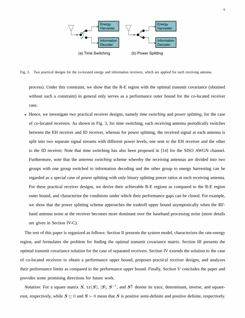
(b) Power Splitting(a) Time Switching (b) Power Splitting

Fig. 3. Two practical designs for the co-located energy and information receivers, which are applied for each receivingantenna.

process). Under this constraint, we show that the R-E regionwith the optimal transmit covariance (obtained

without such a constraint) in general only serves as a performance outer bound for the co-located receiver

case.

• Hence, we investigate two practical receiver designs, namely time switchingandpower splitting, for the case

of co-located receivers. As shown in Fig. 3, for time switching, each receiving antenna periodically switches

between the EH receiver and ID receiver, whereas for power splitting, the received signal at each antenna is

split into two separate signal streams with different powerlevels, one sent to the EH receiver and the other

to the ID receiver. Note that time switching has also been proposed in [14] for the SISO AWGN channel.

Furthermore, note that theantenna switchingscheme whereby the receiving antennas are divided into two

groups with one group switched to information decoding and the other group to energy harvesting can be

regarded as a special case of power splitting with only binary splitting power ratios at each receiving antenna.

For these practical receiver designs, we derive their achievable R-E regions as compared to the R-E region

outer bound, and characterize the conditions under which their performance gaps can be closed. For example,

we show that the power splitting scheme approaches the tradeoff upper bound asymptotically when the RF-

band antenna noise at the receiver becomes more dominant over the baseband processing noise (more details

are given in Section IV-C).

The rest of this paper is organized as follows: Section II presents the system model, characterizes the rate-energy

region, and formulates the problem for finding the optimal transmit covariance matrix. Section III presents the

optimal transmit covariance solution for the case of separated receivers. Section IV extends the solution to the case

of co-located receivers to obtain a performance upper bound, proposes practical receiver designs, and analyzes

their performance limits as compared to the performance upper bound. Finally, Section V concludes the paper and

provides some promising directions for future work.

Notation: For a square matrixS, tr(S), |S|, S−1, andS1

2 denote its trace, determinant, inverse, and square-

root, respectively, whileS 0 andS ≻ 0 mean thatS is positive semi-definite and positive definite, respectively.

7

For an arbitrary-size matrixM , MH andMT denote the conjugate transpose and transpose ofM , respectively.

diag(x1, . . . , xM ) denotes anM × M diagonal matrix withx1, . . . , xM being the diagonal elements.I and 0

denote an identity matrix and an all-zero vector, respectively, with appropriate dimensions.E[·] denotes the statistical

expectation. The distribution of a circularly symmetric complex Gaussian (CSCG) random vector with meanx and

covariance matrixΣ is denoted byCN (x,Σ), and∼ stands for “distributed as”.Cx×y denotes the space ofx× y

matrices with complex entries.‖z‖ is the Euclidean norm of a complex vectorz, and|z| is the absolute value of

a complex scalarz. max(x, y) andmin(x, y) denote the maximum and minimum between two real numbers,x

andy, respectively, and(x)+ = max(x, 0). All the log(·) functions have base-2 by default.

II. SYSTEM MODEL AND PROBLEM FORMULATION

As shown in Fig. 2, this paper considers a wireless broadcastsystem consisting of one transmitter, one EH

receiver, and one ID receiver. It is assumed that the transmitter is equipped withM ≥ 1 transmitting antennas, and

the EH receiver and the ID receiver are equipped withNEH ≥ 1 andNID ≥ 1 receiving antennas, respectively. In

addition, it is assumed that the transmitter and both receivers operate over the same frequency band. Assuming a

narrow-band transmission over quasi-static fading channels, the baseband equivalent channels from the transmitter

to the EH receiver and ID receiver can be modeled by matricesG ∈ CNEH×M andH ∈ CNID×M , respectively.

It is assumed that at each fading state,G andH are both known at the transmitter, and separately known at the

corresponding receiver. Note that for the case of co-located EH and ID receivers,G is identical toH and thus

NEH = NID.

It is worth noting that the EH receiver does not need to convert the received signal from the RF band to the

baseband in order to harvest the carried energy. Nevertheless, thanks to the law of energy conservation, it can be

assumed that the total harvested RF-band power (energy normalized by the baseband symbol period), denoted by

Q, from all receiving antennas at the EH receiver is proportional to that of the received baseband signal, i.e.,

Q = ζE[‖Gx(n)‖2] (1)

whereζ is a constant that accounts for the loss in the energy transducer for converting the harvested energy to

electrical energy to be stored; for the convenience of analysis, it is assumed thatζ = 1 in this paper unless stated

otherwise. We usex(n) ∈ CM×1 to denote the baseband signal broadcast by the transmitter at the nth symbol

interval, which is assumed to be random overn, without loss of generality. The expectation in (1) is thus used to

compute the average power harvested by the EH receiver at each fading state. Note that for simplicity, we assumed

in (1) that the harvested energy due to the background noise at the EH receiver is negligible and thus can be

8

ignored.2

On the other hand, the baseband transmission from the transmitter to the ID receiver can be modeled by

y(n) = Hx(n) + z(n) (2)

wherey(n) ∈ CNID×1 denotes the received signal at thenth symbol interval, andz(n) ∈ CNID×1 denotes the

receiver noise vector. It is assumed thatz(n)’s are independent overn andz(n) ∼ CN (0, I). Under the assumption

that x(n) is random overn, we useS = E[x(n)xH(n)] to denote the covariance matrix ofx(n). In addition,

we assume that there is an average power constraint at the transmitter across all transmitting antennas denoted

by E[‖x(n)‖2] = tr(S) ≤ P . In the following, we examine the optimal transmit covarianceS to maximize the

transported energy efficiency and information rate to the EHand ID receivers, respectively.

Consider first the MIMO link from the transmitter to the EH receiver when the ID receiver is not present. In

this case, the design objective forS is to maximize the powerQ received at the EH receiver. Since from (1) it

follows thatQ = tr(GSGH) with ζ = 1, the aforementioned design problem can be formulated as

(P1) maxS

Q := tr(

GSGH)

s.t. tr(S) ≤ P,S 0.

Let T1 = min(M,NEH) and the (reduced) singular value decomposition (SVD) ofG be denoted byG =

UGΓ1/2G V H

G , whereUG ∈ CNEH×T1 and V G ∈ CM×T1 , each of which consists of orthogonal columns with

unit norm, andΓG = diag(g1, . . . , gT1) with g1 ≥ g2 ≥ . . . ≥ gT1

≥ 0. Furthermore, letv1 denote the first

column ofV G. Then, we have the following proposition.

Proposition2.1: The optimal solution to (P1) isSEH = Pv1vH1 .

Proof: See Appendix A.

GivenS = SEH, it follows that the maximum harvested power at the EH receiver is given byQmax = g1P . It is

worth noting that sinceSEH is a rank-one matrix, the maximum harvested power is achieved by beamformingat

the transmitter, which aligns with the strongest eigenmodeof the matrixGHG, i.e., the transmitted signal can be

written asx(n) =√Pv1s(n), wheres(n) is an arbitrary random signal overn with zero mean and unit variance,

andv1 is the transmit beamforming vector. For convenience, we name the above transmit beamforming scheme

to maximize the efficiency of WPT as “energy beamforming”.

Next, consider the MIMO link from the transmitter to the ID receiver without the presence of any EH receiver.

Assuming the optimal Gaussian codebook at the transmitter,i.e., x(n) ∼ CN (0,S), the transmit covarianceS to

2The results of this paper are readily extendible to study theimpacts of non-negligible background noise and/or co-channel interference

on the SWIPT system performance.

9

maximize the transmission rate over this MIMO channel can beobtained by solving the following problem [13]:

(P2) maxS

R := log |I +HSHH |

s.t. tr(S) ≤ P,S 0.

The optimal solution to the above problem is known to have thefollowing form [13]: SID = V HΛV HH , where

V H ∈ CM×T2 is obtained from the (reduced) SVD ofH expressed byH = UHΓ1/2H V H

H , with T2 = min(M,NID),

UH ∈ CNID×T2 , ΓH = diag(h1, . . . , hT2), h1 ≥ h2 ≥ . . . ≥ hT2

≥ 0, andΛ = diag(p1, . . . , pT2) with the

diagonal elements obtained from the standard “water-filling (WF)” power allocation solution [13]:

pi =

(

ν − 1

hi

)+

, i = 1, . . . , T2 (3)

with ν being the so-called (constant) water-level that makes∑T2

i=1 pi = P . The corresponding maximum trans-

mission rate is then given byRmax =∑T2

i=1 log(1 + hipi). The maximum rate is achieved in general byspatial

multiplexing[6] over up toT2 spatially decoupled AWGN channels, together with the Gaussian codebook, i.e., the

transmitted signal can be expressed asx(n) = V HΛ1/2s(n), wheres(n) is a Gaussian random vector∼ CN (0, I),

V H andΛ1/2 denote the precoding matrix and the (diagonal) power allocation matrix, respectively.

Remark2.1: It is worth noting that in Problem (P1), it is assumed that thetransmitter sends to the EH receiver

continuously. Now suppose that the transmitter only transmits a fraction of the total time denoted byα with

0 < α ≤ 1. Furthermore, assume that the transmit power level can be adjusted flexibly provided that the consumed

average power is bounded byP , i.e.,α · tr(S) + (1− α) · 0 ≤ P or tr(S) ≤ P/α. In this case, it can be easily

shown that the transmit covarianceS = (P/α)v1vH1 also achieves the maximum harvested powerQmax = g1P for

any 0 < α ≤ 1, which suggests that the maximum power delivered is independent of transmission time. However,

unlike the case of maximum power transfer, the maximum information rate reliably transmitted to the ID receiver

requires that the transmitter send signals continuously, i.e., α = 1, as assumed in Problem (P2). This can be

easily verified by observing that for any0 < α ≤ 1 andS 0, α log |I + H(S/α)HH | ≤ log |I + HSHH |

where the equality holds only whenα = 1, sinceR is a nonlinear concave function ofS. Thus, to maximize

both power and rate transfer at the same time, the transmitter should broadcast to the EH and ID receivers all the

time. Furthermore, note that the assumed Gaussian distribution for transmitted signals is necessary for achieving

the maximum rate transfer, but not necessary for the maximumpower transfer. In fact, for any arbitrary complex

numberc that satisfies|c| = 1, even a deterministic transmitted signalx(n) =√Pv1c,∀n, achieves the maximum

transferred powerQmax in Problem (P1). However, to maximize simultaneous power and information transfer with

the same transmitted signal, the Gaussian input distribution is sufficient as well as necessary.

Now, consider the case where both the EH and ID receivers are present. From the above results, it is seen that the

10

0 50 100 150 200 2500

0.1

0.2

0.3

0.4

0.5

0.6

0.7

Rate (Mbps)

Ene

rgy

(mW

)

Optimal Transmit Covariance Time−Sharing

(REH

, Qmax

)

(Rmax

, QID

)

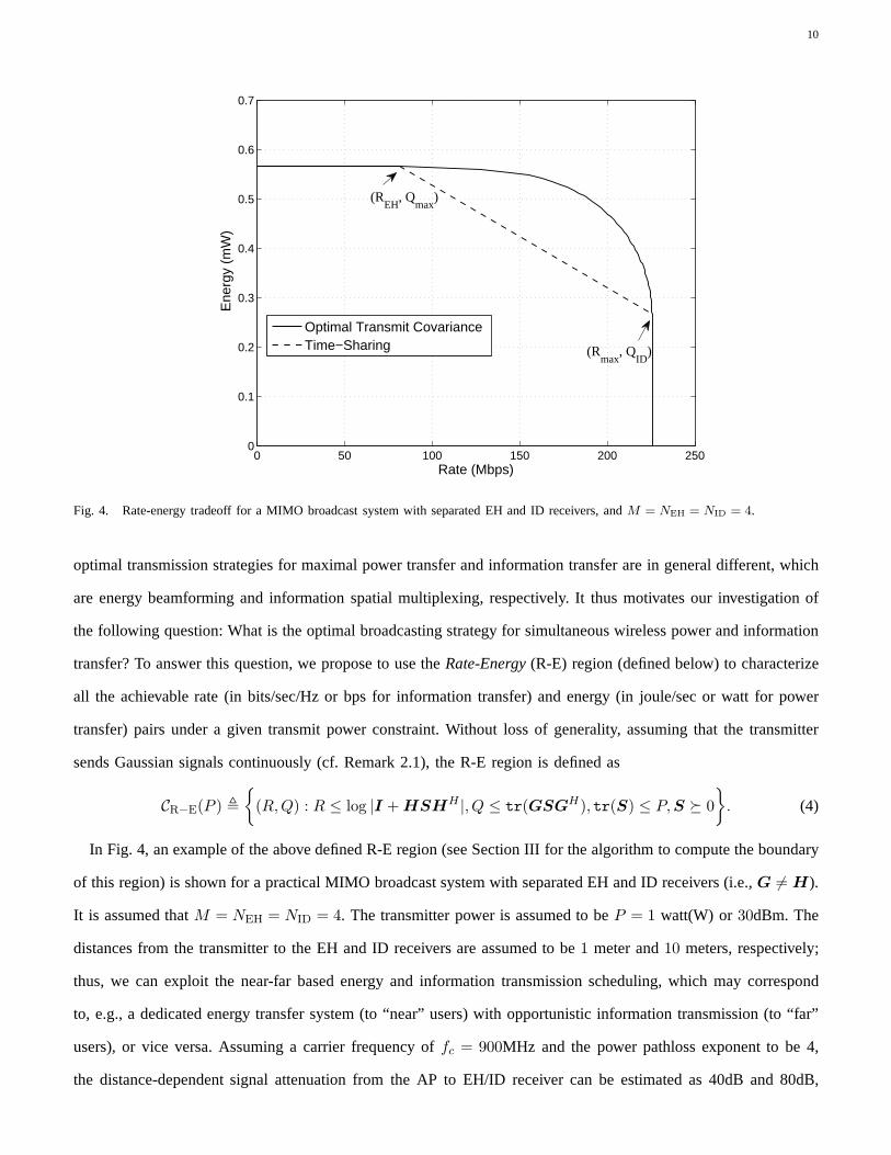
Fig. 4. Rate-energy tradeoff for a MIMO broadcast system with separated EH and ID receivers, andM = NEH = NID = 4.

optimal transmission strategies for maximal power transfer and information transfer are in general different, which

are energy beamforming and information spatial multiplexing, respectively. It thus motivates our investigation of

the following question: What is the optimal broadcasting strategy for simultaneous wireless power and information

transfer? To answer this question, we propose to use theRate-Energy(R-E) region (defined below) to characterize

all the achievable rate (in bits/sec/Hz or bps for information transfer) and energy (in joule/sec or watt for power

transfer) pairs under a given transmit power constraint. Without loss of generality, assuming that the transmitter

sends Gaussian signals continuously (cf. Remark 2.1), the R-E region is defined as

CR−E(P ) ,

(R,Q) : R ≤ log |I +HSHH |, Q ≤ tr(GSGH), tr(S) ≤ P,S 0

. (4)

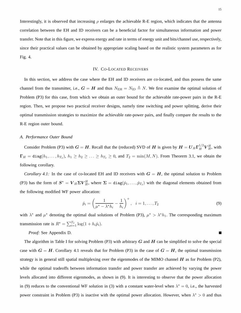
In Fig. 4, an example of the above defined R-E region (see Section III for the algorithm to compute the boundary

of this region) is shown for a practical MIMO broadcast system with separated EH and ID receivers (i.e.,G 6= H).

It is assumed thatM = NEH = NID = 4. The transmitter power is assumed to beP = 1 watt(W) or 30dBm. The

distances from the transmitter to the EH and ID receivers areassumed to be1 meter and10 meters, respectively;

thus, we can exploit the near-far based energy and information transmission scheduling, which may correspond

to, e.g., a dedicated energy transfer system (to “near” users) with opportunistic information transmission (to “far”

users), or vice versa. Assuming a carrier frequency offc = 900MHz and the power pathloss exponent to be 4,

the distance-dependent signal attenuation from the AP to EH/ID receiver can be estimated as 40dB and 80dB,

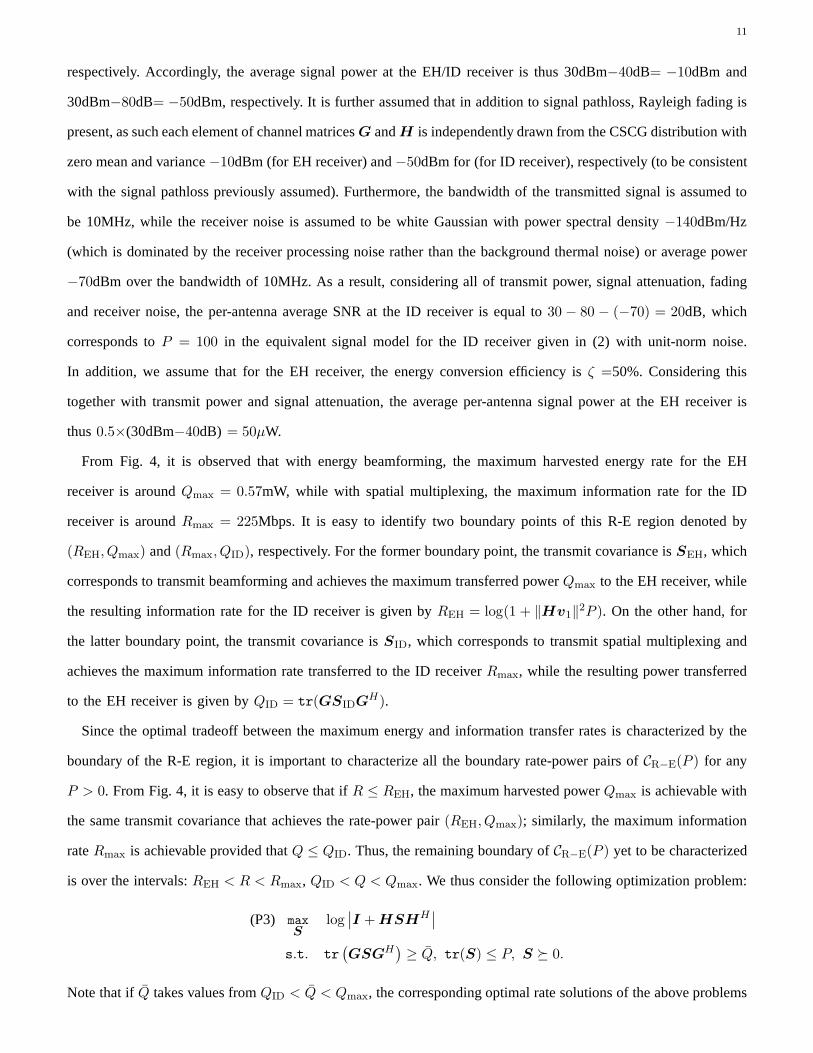
11

respectively. Accordingly, the average signal power at theEH/ID receiver is thus 30dBm−40dB= −10dBm and

30dBm−80dB= −50dBm, respectively. It is further assumed that in addition tosignal pathloss, Rayleigh fading is

present, as such each element of channel matricesG andH is independently drawn from the CSCG distribution with

zero mean and variance−10dBm (for EH receiver) and−50dBm for (for ID receiver), respectively (to be consistent

with the signal pathloss previously assumed). Furthermore, the bandwidth of the transmitted signal is assumed to

be 10MHz, while the receiver noise is assumed to be white Gaussian with power spectral density−140dBm/Hz

(which is dominated by the receiver processing noise ratherthan the background thermal noise) or average power

−70dBm over the bandwidth of 10MHz. As a result, considering allof transmit power, signal attenuation, fading

and receiver noise, the per-antenna average SNR at the ID receiver is equal to30 − 80 − (−70) = 20dB, which

corresponds toP = 100 in the equivalent signal model for the ID receiver given in (2) with unit-norm noise.

In addition, we assume that for the EH receiver, the energy conversion efficiency isζ =50%. Considering this

together with transmit power and signal attenuation, the average per-antenna signal power at the EH receiver is

thus0.5×(30dBm−40dB) = 50µW.

From Fig. 4, it is observed that with energy beamforming, themaximum harvested energy rate for the EH

receiver is aroundQmax = 0.57mW, while with spatial multiplexing, the maximum information rate for the ID

receiver is aroundRmax = 225Mbps. It is easy to identify two boundary points of this R-E region denoted by

(REH, Qmax) and(Rmax, QID), respectively. For the former boundary point, the transmitcovariance isSEH, which

corresponds to transmit beamforming and achieves the maximum transferred powerQmax to the EH receiver, while

the resulting information rate for the ID receiver is given by REH = log(1 + ‖Hv1‖2P ). On the other hand, for

the latter boundary point, the transmit covariance isSID, which corresponds to transmit spatial multiplexing and

achieves the maximum information rate transferred to the IDreceiverRmax, while the resulting power transferred

to the EH receiver is given byQID = tr(GSIDGH).

Since the optimal tradeoff between the maximum energy and information transfer rates is characterized by the

boundary of the R-E region, it is important to characterize all the boundary rate-power pairs ofCR−E(P ) for any

P > 0. From Fig. 4, it is easy to observe that ifR ≤ REH, the maximum harvested powerQmax is achievable with

the same transmit covariance that achieves the rate-power pair (REH, Qmax); similarly, the maximum information

rateRmax is achievable provided thatQ ≤ QID. Thus, the remaining boundary ofCR−E(P ) yet to be characterized

is over the intervals:REH < R < Rmax, QID < Q < Qmax. We thus consider the following optimization problem:

(P3) maxS

log∣

∣I +HSHH∣

∣

s.t. tr(

GSGH)

≥ Q, tr(S) ≤ P, S 0.

Note that ifQ takes values fromQID < Q < Qmax, the corresponding optimal rate solutions of the above problems

12

are the boundary rate points of the R-E region overREH < R < Rmax. Notice that the transmit covariance solutions

to the above problems in general yield larger rate-power pairs than those by simply “time-sharing” the optimal

transmit covariance matricesSEH andSID for EH and ID receivers separately (see the dashed line in Fig. 4).3

Problem (P3) is a convex optimization problem, since its objective function is concave overS and its constraints

specify a convex set ofS. Note that (P3) resembles a similar problem formulated in [15], [16] (see also [17] and

references therein) under the cognitive radio (CR) setup, where the rate of a secondary MIMO link is maximized

subject to a set of so-calledinterference power constraintsto protect the co-channel primary receivers. However,

there is a key difference between (P3) and the problem in [16]: the harvested power constraint in (P3) has the

reversed inequality of that of the interference power constraint in [16], since in our case it is desirable for the

EH receiver to harvest more power from the transmitter, as opposed to that in [16] the interference power at the

primary receiver should be minimized. As such, it is not immediately clear whether the solution in [16] can be

directly applied for solving (P3) with the reversed power inequality. In the following, we will examine the solutions

to Problem (P3) for the two cases with arbitraryG andH (the case of separated receivers) andG = H (the case

of co-located receivers), respectively.

III. SEPARATED RECEIVERS

Consider the case where the EH receiver and ID receiver are spatially separated and thus in general have different

channels from the transmitter. In this section, we first solve Problem (P3) with arbitraryG andH and derive a

semi-closed-form expression for the optimal transmit covariance. Then, we examine the optimal solution for the

special case of MISO channels from the transmitter to ID and/or EH receivers.

Since Problem (P3) is convex and satisfies the Slater’s condition [18], it has a zero duality gap and thus can

be solved using the Lagrange duality method.4 Thus, we introduce two non-negative dual variables,λ and µ,

associated with the harvested power constraint and transmit power constraint in (P3), respectively. The optimal

solution to Problem (P3) is then given by the following theorem in terms ofλ∗ andµ∗, which are the optimal

dual solutions of Problem (P3) (see Appendix B for details).Note that for Problem (P3), given any pair ofQ

(QID < Q < Qmax) andP > 0, there exists one unique pair ofλ∗ > 0 andµ∗ > 0.

Theorem3.1: The optimal solution to Problem (P3) has the following form:

S∗ = A−1/2V ΛVHA−1/2 (5)

3By time-sharing, we mean that the AP transmits simultaneously to both EH and ID receivers with the energy-maximizing transmit

covarianceSEH (i.e. energy beamforming) forβ portion of each block time, and the information-rate-maximizing transmit covarianceSID

(i.e. spatial multiplexing) for the remaining1− β portion of each block time, with0 ≤ β ≤ 1.4It is worth noting that Problem (P3) is convex and thus can be solved efficiently by the interior point method [18]; in this paper, we

apply the Lagrange duality method for this problem mainly toreveal the optimal precoder structure.

13

whereA = µ∗I − λ∗GHG, V ∈ CM×T2 is obtained from the (reduced) SVD of the matrixHA−1/2 given by

HA−1/2 = U Γ1/2

VH

, with Γ = diag(h1, . . . , hT2), h1 ≥ h2 ≥ . . . ≥ hT2

≥ 0, and Λ = diag(p1, . . . , pT2),

with pi = (1− 1/hi)+, i = 1, . . . , T2.

Proof: See Appendix B.

Note that this theorem requires thatA = µ∗I − λ∗GHG ≻ 0, implying thatµ∗ > λ∗g1 (recall thatg1 is the

largest eigenvalue of matrixGHG), which is not present for a similar result in [17] under the CR setup with

the reversed interference power constraint. One algorithmthat can be used to solve (P3) is provided in Table

I of Appendix B. From Theorem 3.1, the maximum transmission rate for Problem (P3) can be shown to be

R∗ = log∣

∣I +HS∗HH∣

∣ =∑T2

i=1 log(1 + hipi), for which the proof is omitted here for brevity.

Next, we examine the optimal solution to Problem (P3) for thespecial case where the ID receiver has one single

antenna, i.e.,NID = 1, and thus the MIMO channelH reduces to a row vectorhH with h ∈ CM×1. Suppose

that the EH receiver is still equipped withNEH ≥ 1 antennas, and thus the MIMO channelG remains unchanged.

From Theorem 3.1, we obtain the following corollary.

Corollary 3.1: In the case of MISO channel from the transmitter to ID receiver, i.e., H ≡ hH , the optimal

solution to Problem (P3) reduces to the following form:

S∗ = A−1h

(

1

‖A−1/2h‖2− 1

‖A−1/2h‖4

)+

hHA−1 (6)

whereA = µ∗I−λ∗GHG, with λ∗ andµ∗ denoting the optimal dual solutions of Problem (P3). Correspondingly,

the optimal value of (P3) isR∗ =(

2 log(

‖A−1/2h‖))+

.

Proof: See Appendix C.

From (6), it is observed that the optimal transmit covariance is a rank-onematrix, from which it follows that

beamformingis the optimal transmission strategy in this case, where thetransmit beamforming vector should be

aligned with the vectorA−1h. Moreover, consider the case where both channels from the transmitter to ID/EH

receivers are MISO, i.e.,H ≡ hH , andG ≡ gH with g ∈ CM×1. From Corollary 3.1, it follows immediately

that the optimal covariance solution to Problem (P3) is still beamforming. In the following theorem, we show a

closed-form solution of the optimal beamforming vector at the transmitter for this special case, which differs from

the semi-closed-form solution (6) that was expressed in terms of dual variables.

Theorem3.2: In the case of MISO channels from transmitter to both ID and EHreceivers, i.e.,H ≡ hH , and

G ≡ gH , the optimal solution to Problem (P3) can be expressed asS∗ = PvvH , where the beamforming vector

v has a unit-norm and is given by

v =

h 0 ≤ Q ≤ |gH h|2P√

QP‖g‖2 e

j∠αgh g +√

1− QP‖g‖2 hg⊥ |gHh|2P < Q ≤ P‖g‖2

(7)

14

0 0.5 1 1.5 2 2.5 3 3.50

1

2

3

4

5

6

7

8

9

10

11

Rate (bits/channel use)

Ene

rgy

Uni

t

ρ=0.9ρ=0.5ρ=0.1

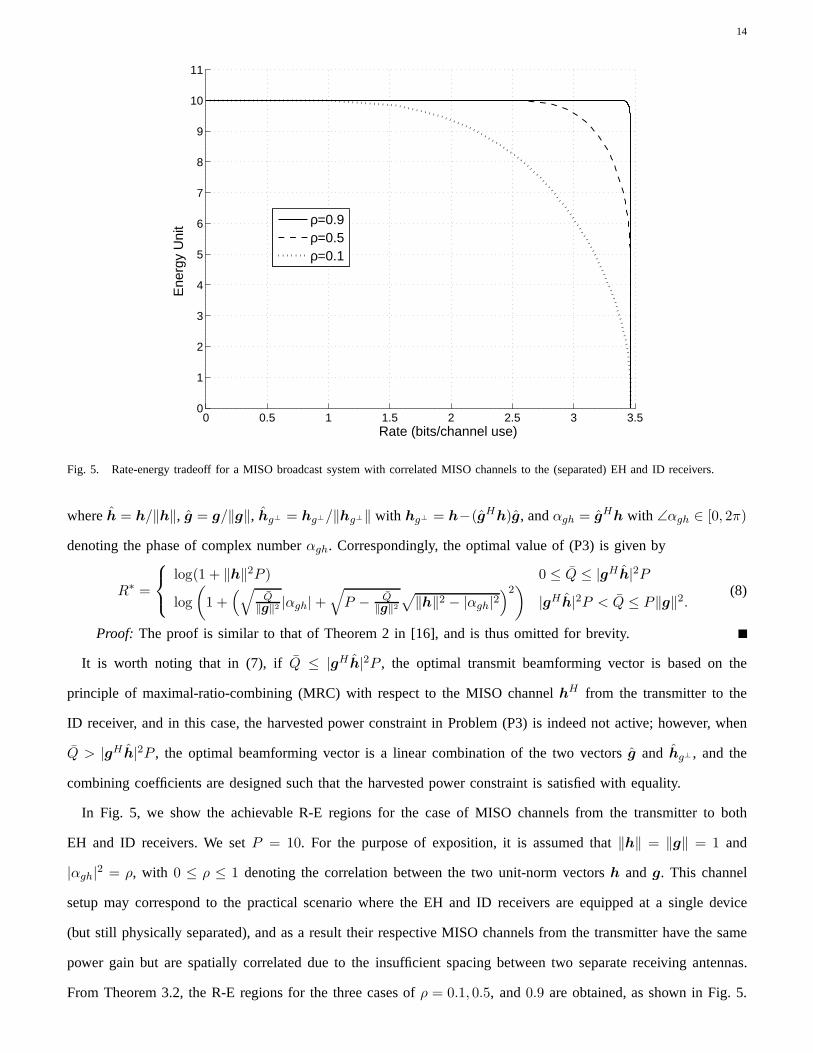
Fig. 5. Rate-energy tradeoff for a MISO broadcast system with correlated MISO channels to the (separated) EH and ID receivers.

whereh = h/‖h‖, g = g/‖g‖, hg⊥ = hg⊥/‖hg⊥‖ with hg⊥ = h−(gHh)g, andαgh = gHh with ∠αgh ∈ [0, 2π)

denoting the phase of complex numberαgh. Correspondingly, the optimal value of (P3) is given by

R∗ =

log(1 + ‖h‖2P ) 0 ≤ Q ≤ |gHh|2Plog

(

1 +(√

Q‖g‖2 |αgh|+

√

P − Q‖g‖2

√

‖h‖2 − |αgh|2)2)

|gHh|2P < Q ≤ P‖g‖2.(8)

Proof: The proof is similar to that of Theorem 2 in [16], and is thus omitted for brevity.

It is worth noting that in (7), ifQ ≤ |gH h|2P , the optimal transmit beamforming vector is based on the

principle of maximal-ratio-combining (MRC) with respect to the MISO channelhH from the transmitter to the

ID receiver, and in this case, the harvested power constraint in Problem (P3) is indeed not active; however, when

Q > |gH h|2P , the optimal beamforming vector is a linear combination of the two vectorsg and hg⊥ , and the

combining coefficients are designed such that the harvestedpower constraint is satisfied with equality.

In Fig. 5, we show the achievable R-E regions for the case of MISO channels from the transmitter to both

EH and ID receivers. We setP = 10. For the purpose of exposition, it is assumed that‖h‖ = ‖g‖ = 1 and

|αgh|2 = ρ, with 0 ≤ ρ ≤ 1 denoting the correlation between the two unit-norm vectorsh and g. This channel

setup may correspond to the practical scenario where the EH and ID receivers are equipped at a single device

(but still physically separated), and as a result their respective MISO channels from the transmitter have the same

power gain but are spatially correlated due to the insufficient spacing between two separate receiving antennas.

From Theorem 3.2, the R-E regions for the three cases ofρ = 0.1, 0.5, and0.9 are obtained, as shown in Fig. 5.

15

Interestingly, it is observed that increasingρ enlarges the achievable R-E region, which indicates that the antenna

correlation between the EH and ID receivers can be a beneficial factor for simultaneous information and power

transfer. Note that in this figure, we express energy and ratein terms of energy unit and bits/channel use, respectively,

since their practical values can be obtained by appropriatescaling based on the realistic system parameters as for

Fig. 4.

IV. CO-LOCATED RECEIVERS

In this section, we address the case where the EH and ID receivers are co-located, and thus possess the same

channel from the transmitter, i.e.,G = H and thusNEH = NID , N . We first examine the optimal solution of

Problem (P3) for this case, from which we obtain an outer bound for the achievable rate-power pairs in the R-E

region. Then, we propose two practical receiver designs, namely time switching and power splitting, derive their

optimal transmission strategies to maximize the achievable rate-power pairs, and finally compare the results to the

R-E region outer bound.

A. Performance Outer Bound

Consider Problem (P3) withG = H . Recall that the (reduced) SVD ofH is given byH = UHΓ1/2H V H

H , with

ΓH = diag(h1, . . . , hT2), h1 ≥ h2 ≥ . . . ≥ hT2

≥ 0, andT2 = min(M,N). From Theorem 3.1, we obtain the

following corollary.

Corollary 4.1: In the case of co-located EH and ID receivers withG = H , the optimal solution to Problem

(P3) has the form ofS∗ = V HΣV HH , whereΣ = diag(p1, . . . , pT2

) with the diagonal elements obtained from

the following modified WF power allocation:

pi =

(

1

µ∗ − λ∗hi− 1

hi

)+

, i = 1, . . . , T2 (9)

with λ∗ andµ∗ denoting the optimal dual solutions of Problem (P3),µ∗ > λ∗h1. The corresponding maximum

transmission rate isR∗ =∑T2

i=1 log(1 + hipi).

Proof: See Appendix D.

The algorithm in Table I for solving Problem (P3) with arbitraryG andH can be simplified to solve the special

case withG = H . Corollary 4.1 reveals that for Problem (P3) in the case ofG = H , the optimal transmission

strategy is in general still spatial multiplexing over the eigenmodes of the MIMO channelH as for Problem (P2),

while the optimal tradeoffs between information transfer and power transfer are achieved by varying the power

levels allocated into different eigenmodes, as shown in (9). It is interesting to observe that the power allocation

in (9) reduces to the conventional WF solution in (3) with a constant water-level whenλ∗ = 0, i.e., the harvested

power constraint in Problem (P3) is inactive with the optimal power allocation. However, whenλ∗ > 0 and thus

16

the harvested power constraint is active corresponding to the Pareto-optimal regime of our interest, the power

allocation in (9) is observed to have anon-decreasingwater-level ashi’s increase. Note that this modified WF

policy has also been shown in [2] for power allocation in frequency-selective AWGN channels.

Using Corollary 4.1, we can characterize all the boundary points of the R-E regionCR−E(P ) defined in (4) for the

case of co-located receivers withG = H . For example, if the total transmit power is allocated to thechannel with

the largest gainh1, i.e., p1 = P andpi = 0, i = 2, . . . , T2, the maximum harvested powerQmax = Ph1 is achieved

by transmit beamforming. On the other hand, if transmit spatial multiplexing is applied with the conventional WF

power allocation given in (9) withλ∗ = 0, the correspondingR∗ becomes the maximum transmission rate,Rmax.

However, unlike the case of separated EH and ID receivers in which the entire boundary ofCR−E(P ) is achievable,

in the case of co-located receivers, except the two boundaryrate-power pairs(Rmax, 0) and(0, Qmax), all the other

boundary pairs ofCR−E(P ) may not be achievable in practice. Note that these boundary points are achievable

if and only if (iff) the following premise is true: the power of the received signal across all antennas is totally

harvested, and at the same time the carried information witha transmission rate up to the MIMO channel capacity

(for a given transmit covariance) is decodable. However, existing EH circuits are not yet able to directly decode

the information carried in the RF-band signal, even for the SISO channel case; as a result, how to achieve the

remaining boundary rate-power pairs ofCR−E(P ) in the MIMO case with the co-located EH and ID receiver

remains an interesting open problem. Therefore, in the caseof co-located receivers, the boundary ofCR−E(P )

given by Corollary 4.1 in general only serves as anouter boundfor the achievable rate-power pairs with practical

receiver designs, as will be investigated in the following subsections.

B. Time Switching

First, as shown in Fig. 3(a), we consider thetime switching(TS) scheme, with which each transmission block

is divided into two orthogonal time slots, one for transferring power and the other for transmitting data. The co-

located EH and ID receiver switches its operations periodically between harvesting energy and decoding information

between the two time slots. It is assumed that time synchronization has been perfectly established between the

transmitter and the receiver, and thus the receiver can synchronize its function switching with the transmitter. With

orthogonal transmissions, the transmitted signals for theEH receiver and ID receiver can be designed separately,

but subject to a total transmit power constraint. Letα with 0 ≤ α ≤ 1 denote the percentage of transmission time

allocated to the EH time slot. We then consider the followingtwo types of power constraints at the transmitter:

• Fixed power constraint: The transmitted signals to the ID and EH receivers have the same fixed power

constraint given bytr(S1) ≤ P , andtr(S2) ≤ P , whereS1 andS2 denote the transmit covariance matrices

for the ID and EH transmission time slots, respectively.

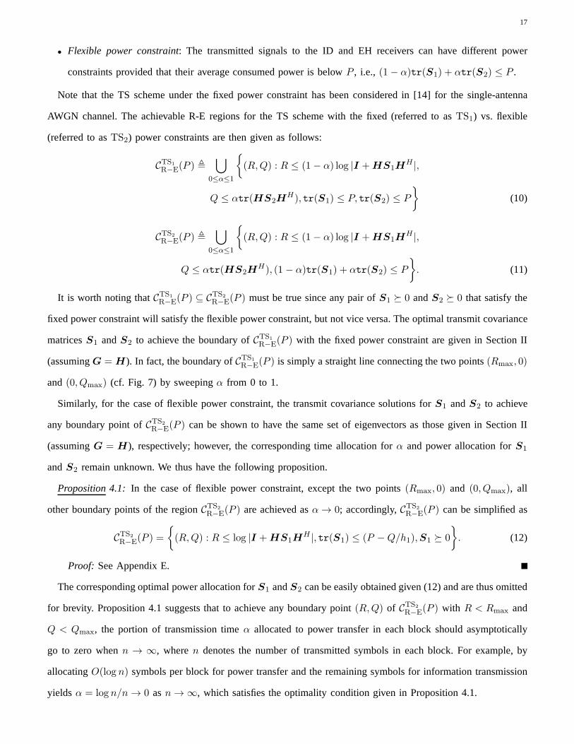
17

• Flexible power constraint: The transmitted signals to the ID and EH receivers can have different power

constraints provided that their average consumed power is below P , i.e., (1− α)tr(S1) + αtr(S2) ≤ P .

Note that the TS scheme under the fixed power constraint has been considered in [14] for the single-antenna

AWGN channel. The achievable R-E regions for the TS scheme with the fixed (referred to asTS1) vs. flexible

(referred to asTS2) power constraints are then given as follows:

CTS1

R−E(P ) ,⋃

0≤α≤1

(R,Q) : R ≤ (1− α) log |I +HS1HH |,

Q ≤ αtr(HS2HH), tr(S1) ≤ P, tr(S2) ≤ P

(10)

CTS2

R−E(P ) ,⋃

0≤α≤1

(R,Q) : R ≤ (1− α) log |I +HS1HH |,

Q ≤ αtr(HS2HH), (1 − α)tr(S1) + αtr(S2) ≤ P

. (11)

It is worth noting thatCTS1

R−E(P ) ⊆ CTS2

R−E(P ) must be true since any pair ofS1 0 andS2 0 that satisfy the

fixed power constraint will satisfy the flexible power constraint, but not vice versa. The optimal transmit covariance

matricesS1 andS2 to achieve the boundary ofCTS1

R−E(P ) with the fixed power constraint are given in Section II

(assumingG = H). In fact, the boundary ofCTS1

R−E(P ) is simply a straight line connecting the two points(Rmax, 0)

and (0, Qmax) (cf. Fig. 7) by sweepingα from 0 to 1.

Similarly, for the case of flexible power constraint, the transmit covariance solutions forS1 andS2 to achieve

any boundary point ofCTS2

R−E(P ) can be shown to have the same set of eigenvectors as those given in Section II

(assumingG = H), respectively; however, the corresponding time allocation for α and power allocation forS1

andS2 remain unknown. We thus have the following proposition.

Proposition4.1: In the case of flexible power constraint, except the two points (Rmax, 0) and (0, Qmax), all

other boundary points of the regionCTS2

R−E(P ) are achieved asα → 0; accordingly,CTS2

R−E(P ) can be simplified as

CTS2

R−E(P ) =

(R,Q) : R ≤ log |I +HS1HH |, tr(S1) ≤ (P −Q/h1),S1 0

. (12)

Proof: See Appendix E.

The corresponding optimal power allocation forS1 andS2 can be easily obtained given (12) and are thus omitted

for brevity. Proposition 4.1 suggests that to achieve any boundary point(R,Q) of CTS2

R−E(P ) with R < Rmax and

Q < Qmax, the portion of transmission timeα allocated to power transfer in each block should asymptotically

go to zero whenn → ∞, wheren denotes the number of transmitted symbols in each block. Forexample, by

allocatingO(log n) symbols per block for power transfer and the remaining symbols for information transmission

yieldsα = log n/n → 0 asn → ∞, which satisfies the optimality condition given in Proposition 4.1.

18

EH ReceiverPower

ρ

ID Receiver

Power

Splitter

)(tnA

)(tnP

ρ−1

(a) Co-located receivers with a power splitter

)(tnA

)(tnP

ID Receiver

(b) ID receiver without a power splitter (b) ID receiver without a power splitter

Fig. 6. Receiver operations with/without a power splitter (the energy harvested due to the receiver noise is ignored forEH receiver).

It is worth noting that the boundary ofCTS2

R−E(P ) in the flexible power constraint case is achieved under the

assumption that the transmitter and receiver can both operate in the regime of infinite power in the EH time slot

due toα → 0, which cannot be implemented with practical power amplifiers. Hence, a more feasible region for

CTS2

R−E(P ) is obtained by adding peak5 transmit power constraints in (11) astr(S1) ≤ Ppeak andtr(S2) ≤ Ppeak,

with Ppeak ≥ P . Similar to Proposition 4.1, it can be shown that the boundary of the achievable R-E region in

this case, denoted byCTS2

R−E(P,Ppeak), is achieved byα = Q/(h1Ppeak). Note that we can equivalently denote the

achievable R-E regionCTS2

R−E(P ) defined in (11) or (12) without any peak power constraint asCTS2

R−E(P,∞).

C. Power Splitting

Next, we propose an alternative receiver design calledpower splitting(PS), whereby the power and information

transfer to the co-located EH and ID receivers are simultaneously achieved via a set of power splitting devices,

one device for each receiving antenna, as shown in Fig. 3(b).In order to gain more insight into the PS scheme, we

consider first the simple case of a single-antenna AWGN channel with co-located ID and EH receivers, which is

shown in Fig. 6(a). For the ease of comparison, the case of solely information transfer with one single ID receiver

is also shown in Fig. 6(b).

The receiver operations in Fig. 6(a) are explained as follows: The received signal from the antenna is first

corrupted by a Gaussian noise denoted bynA(t) at the RF-band, which is assumed to have zero mean and

equivalent baseband powerσ2A. The RF-band signal is then fed into a power splitter, which is assumed to be

perfect without any noise induced. After the power splitter, the portion of signal power split to the EH receiver is

5Note that the peak power constraint in this context is different from the signal amplitude constraint considered in [1],[14].

19

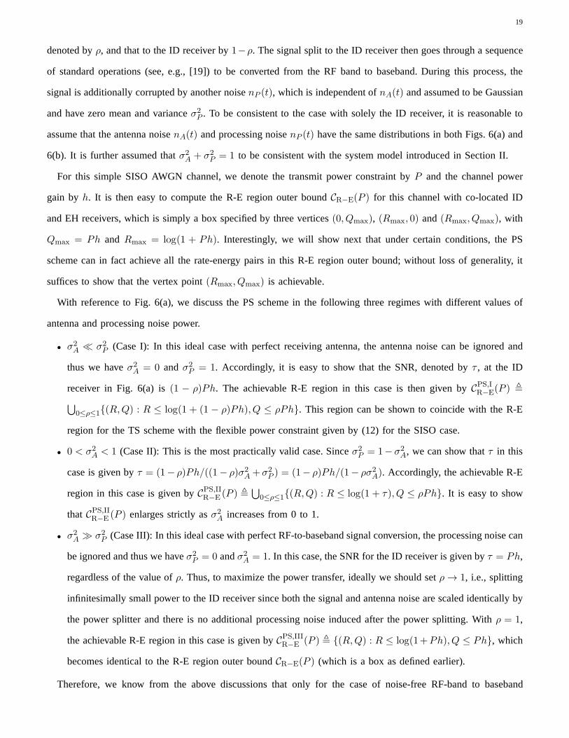
denoted byρ, and that to the ID receiver by1−ρ. The signal split to the ID receiver then goes through a sequence

of standard operations (see, e.g., [19]) to be converted from the RF band to baseband. During this process, the

signal is additionally corrupted by another noisenP (t), which is independent ofnA(t) and assumed to be Gaussian

and have zero mean and varianceσ2P . To be consistent to the case with solely the ID receiver, it is reasonable to

assume that the antenna noisenA(t) and processing noisenP (t) have the same distributions in both Figs. 6(a) and

6(b). It is further assumed thatσ2A + σ2

P = 1 to be consistent with the system model introduced in SectionII.

For this simple SISO AWGN channel, we denote the transmit power constraint byP and the channel power

gain byh. It is then easy to compute the R-E region outer boundCR−E(P ) for this channel with co-located ID

and EH receivers, which is simply a box specified by three vertices(0, Qmax), (Rmax, 0) and(Rmax, Qmax), with

Qmax = Ph and Rmax = log(1 + Ph). Interestingly, we will show next that under certain conditions, the PS

scheme can in fact achieve all the rate-energy pairs in this R-E region outer bound; without loss of generality, it

suffices to show that the vertex point(Rmax, Qmax) is achievable.

With reference to Fig. 6(a), we discuss the PS scheme in the following three regimes with different values of

antenna and processing noise power.

• σ2A ≪ σ2

P (Case I): In this ideal case with perfect receiving antenna,the antenna noise can be ignored and

thus we haveσ2A = 0 andσ2

P = 1. Accordingly, it is easy to show that the SNR, denoted byτ , at the ID

receiver in Fig. 6(a) is(1 − ρ)Ph. The achievable R-E region in this case is then given byCPS,IR−E(P ) ,

⋃

0≤ρ≤1(R,Q) : R ≤ log(1 + (1 − ρ)Ph), Q ≤ ρPh. This region can be shown to coincide with the R-E

region for the TS scheme with the flexible power constraint given by (12) for the SISO case.

• 0 < σ2A < 1 (Case II): This is the most practically valid case. Sinceσ2

P = 1−σ2A, we can show thatτ in this

case is given byτ = (1− ρ)Ph/((1− ρ)σ2A +σ2

P ) = (1− ρ)Ph/(1− ρσ2A). Accordingly, the achievable R-E

region in this case is given byCPS,IIR−E (P ) ,

⋃

0≤ρ≤1(R,Q) : R ≤ log(1 + τ), Q ≤ ρPh. It is easy to show

that CPS,IIR−E (P ) enlarges strictly asσ2

A increases from 0 to 1.

• σ2A ≫ σ2

P (Case III): In this ideal case with perfect RF-to-baseband signal conversion, the processing noise can

be ignored and thus we haveσ2P = 0 andσ2

A = 1. In this case, the SNR for the ID receiver is given byτ = Ph,

regardless of the value ofρ. Thus, to maximize the power transfer, ideally we should setρ → 1, i.e., splitting

infinitesimally small power to the ID receiver since both thesignal and antenna noise are scaled identically by

the power splitter and there is no additional processing noise induced after the power splitting. Withρ = 1,

the achievable R-E region in this case is given byCPS,IIIR−E (P ) , (R,Q) : R ≤ log(1+Ph), Q ≤ Ph, which

becomes identical to the R-E region outer boundCR−E(P ) (which is a box as defined earlier).

Therefore, we know from the above discussions that only for the case of noise-free RF-band to baseband

20

processing (i.e., Case III), the PS scheme achieves the R-E region outer bound and is thus optimal. However, in

practice, such a condition can never be met perfectly, and thus the R-E region outer boundCR−E(P ) is in general

still non-achievable with practical PS receivers. In the following, we will study further the achievable R-E region

by the PS scheme for the more general case of MIMO channels. Itis not difficult to show that if each receiving

antenna satisfies the condition in Case III, the R-E region outer boundCR−E(P ) defined in (4) withG = H is

achievable for the MIMO case by the PS scheme (with each receiving antenna to setρ = 1). For a more practical

purpose, we consider in the rest of this section the “worst” case performance of the PS scheme (i.e., Case I in

the above), when the noiseless antenna is assumed (which leads to the smallest R-E region for the SISO AWGN

channel case). The obtained R-E region will thus provide theperformance lower bound for the PS scheme with

practical receiver circuits. In this case, since there is noantenna noise and the processing noise is added after

the power splitting, it is equivalent to assume that the aggregated receiver noise power remains unchanged with

a power splitter at each receiving antenna. Letρi with 0 ≤ ρi ≤ 1 denote the portion of power split to the EH

receiver at theith receiving antenna,1 ≤ i ≤ N . The achievable R-E region for the PS scheme (in the worst case)

is thus given by

CPSR−E(P ) ,

⋃

0≤ρi≤1,∀i

(R,Q) : R ≤ log |I + Λ1/2ρ HSHH

Λ1/2ρ |, Q ≤ tr(ΛρHSHH), tr(S) ≤ P,S 0

(13)

whereΛρ = diag(ρ1, . . . , ρN ), andΛρ = I −Λρ.

Note that the two points(Rmax, 0) and (0, Qmax) on the boundary ofCPSR−E(P ) can be simply achieved with

ρi = 0,∀i, andρi = 1,∀i, respectively, with the corresponding transmit covariance matrices given in Section II

(with G = H), similar to the TS case. All the other boundary points ofCPSR−E(P ) can be obtained as follows: Let

H ′ = Λ1/2ρ H , G′ = Λ

1/2ρ H , andRPS

R−E(P, ρi) denote the achievable R-E region with PS for a given set of

ρi’s. Then, we can obtain the boundary ofRPSR−E(P, ρi) by solving similar problems like Problem (P3) (with

H andG replaced byH ′ andG′, respectively). Finally, the boundary ofCPSR−E(P ) can be obtained by taking a

union operation over differentRPS(P, ρi)’s with all possibleρi’s.

In particular, we consider two special cases of the PS scheme: i) Uniform Power Splitting(UPS) withρi = ρ,∀i,

and0 ≤ ρ ≤ 1; and ii) On-Off Power Splittingwith ρi ∈ 0, 1,∀i, i.e., ρi taking the value of either 0 or 1. For

the case of on-off power splitting, letΩ ⊆ 1, . . . , N denote one subset of receiving antennas withρi = 1; then

Ω = 1, . . . , N − Ω denotes the other subset of receiving antennas withρi = 0. Clearly,Ω and Ω specify the

sets of receiving antennas switched to EH and ID receivers, respectively; thus, the on-off power splitting is also

termedAntenna Switching(AS).

Let RUPS(P, ρ) denote the achievable R-E region for the UPS scheme with any fixedρ, andCUPSR−E(P ) be the R-E

21

region by taking the union of allRUPS(P, ρ)’s over0 ≤ ρ ≤ 1. Furthermore, letRAS(P,Ω) denote the achievable

R-E region for the AS (or On-Off Power Splitting) scheme witha given pair ofΩ andΩ. It is not difficult to see

that for anyP > 0, CUPSR−E(P ) ⊆ CPS

R−E(P ), andRAS(P,Ω) ⊆ CPSR−E(P ),∀Ω, while CUPS

R−E(P ) = CPSR−E(P ) for the

case of MISO/SISO channel ofH . Moreover, the following proposition shows that for the case of SIMO channel

of H , CUPSR−E(P ) = CPS

R−E(P ) is also true.

Proposition4.2: In the case of co-located EH and ID receivers with a SIMO channel H ≡ h ∈ CN×1, for any

P ≥ 0, CUPSR−E(P ) = CPS

R−E(P ) = (R,Q) : R ≤ log(1 + (‖h‖2P −Q)), 0 ≤ Q ≤ ‖h‖2P.

Proof: See Appendix F.

D. Performance Comparison

The following proposition summarizes the performance comparison between the TS and UPS schemes.

Proposition4.3: For the co-located EH and ID receivers, with anyP > 0, CTS1

R−E(P ) ⊆ CUPSR−E(P ) ⊆ CTS2

R−E(P ),

while CUPSR−E(P ) = CTS2

R−E(P ) iff P ≤ (1/h2 − 1/h1).

Proof: See Appendix G.

From the above proposition, it follows that the TS scheme with the fixed power constraint performs worse than

the UPS scheme in terms of achievable rate-energy pairs. However, the UPS scheme in general performs worse

than the TS scheme under the flexible power constraint (without any peak power constraint), while they perform

identically iff the conditionP ≤ (1/h2 − 1/h1) is satisfied. This may occur when, e.g.,P is sufficiently small

(unlikely in our model since high SNR is of interest), orh2 = 0 (i.e., H is MISO or SIMO). Note that the

performance comparison between the TS scheme (with the flexible power constraint) and the PS scheme with

arbitrary power splitting (instead of UPS) remains unknowntheoretically.

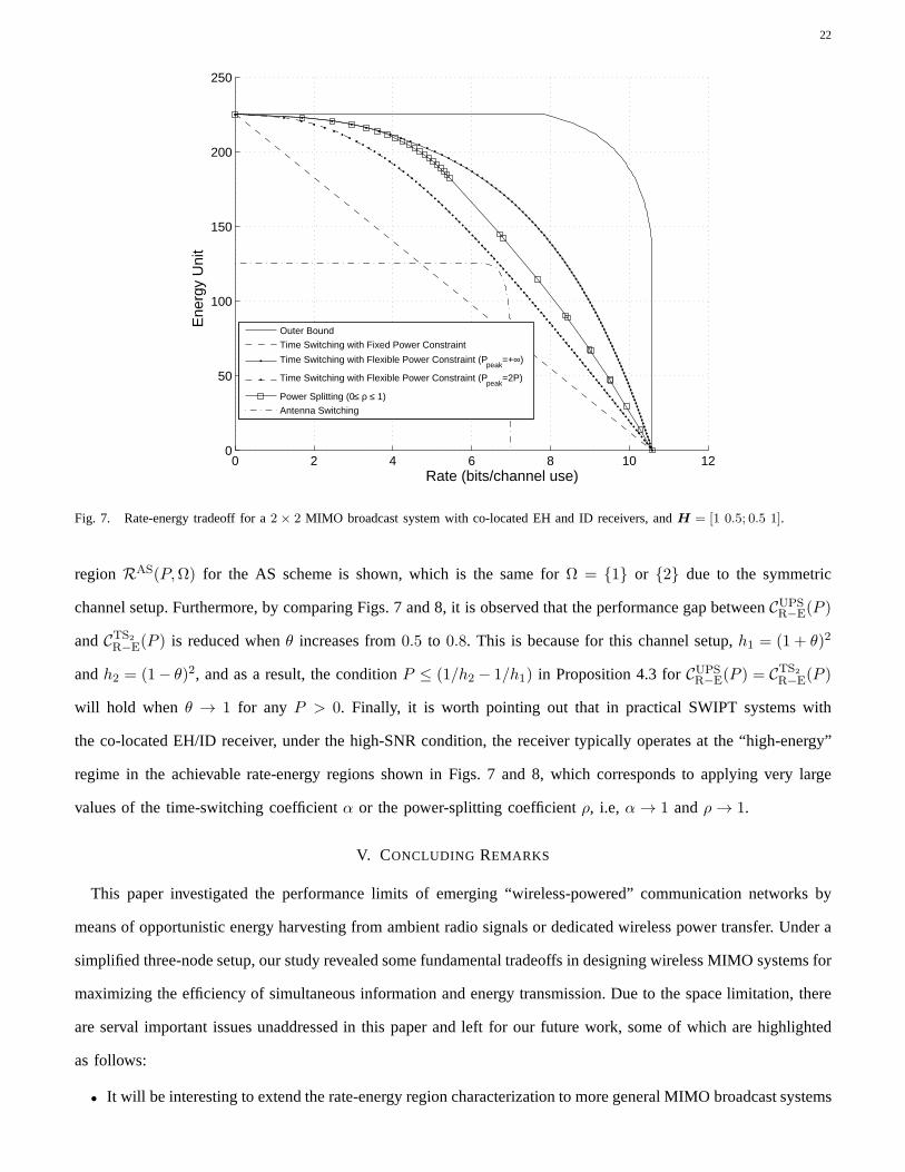
Next, for the purpose of exposition, we compare the rate-energy tradeoff for the case of co-located EH and ID

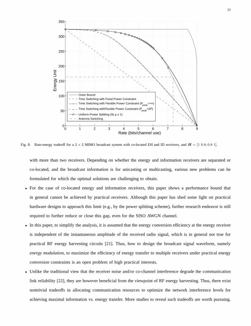
receivers for a symmetric MIMO channelG = H = [1, θ; θ, 1] with θ = 0.5 for Fig. 7 andθ = 0.8 for Fig.

8, respectively. It is assumed thatP = 100. The R-E region outer bound is obtained asCR−E(P ) with G = H

according to Corollary 4.1. The two achievable R-E regions for the TS scheme with fixed vs. flexible power

constraints are shown for comparison, and it is observed that CTS1

R−E(P ) ⊆ CTS2

R−E(P ). The achievable R-E region

for the TS scheme with the flexible power constraintP as well as the peak power constraintPpeak = 2P is also

shown, which is observed to lie betweenCTS1

R−E(P ) andCTS2

R−E(P ). Moreover, the achievable R-E regionCUPSR−E(P )

for the UPS scheme is shown, whose boundary points constitute those ofRUPS(P, ρ)’s with different ρ’s from

0 to 1. It is observed thatCTS1

R−E(P ) ⊆ CUPSR−E(P ) ⊆ CTS2

R−E(P ), which is in accordance with Proposition 4.3. Note

that for this channel, the R-E regionCPSR−E(P ) for the general PS scheme defined in (13) only provides negligible

rate-energy gains overCUPSR−E(P ) by the UPS scheme, and is thus not shown here. In addition, theachievable R-E

22

0 2 4 6 8 10 120

50

100

150

200

250

Rate (bits/channel use)

Ene

rgy

Uni

t

Outer Bound

Time Switching with Fixed Power Constraint

Time Switching with Flexible Power Constraint (Ppeak

=+∞)

Time Switching with Flexible Power Constraint (Ppeak

=2P)

Power Splitting (0≤ ρ ≤ 1)

Antenna Switching

Fig. 7. Rate-energy tradeoff for a2× 2 MIMO broadcast system with co-located EH and ID receivers, and H = [1 0.5; 0.5 1].

region RAS(P,Ω) for the AS scheme is shown, which is the same forΩ = 1 or 2 due to the symmetric

channel setup. Furthermore, by comparing Figs. 7 and 8, it isobserved that the performance gap betweenCUPSR−E(P )

andCTS2

R−E(P ) is reduced whenθ increases from0.5 to 0.8. This is because for this channel setup,h1 = (1 + θ)2

andh2 = (1− θ)2, and as a result, the conditionP ≤ (1/h2 − 1/h1) in Proposition 4.3 forCUPSR−E(P ) = CTS2

R−E(P )

will hold when θ → 1 for any P > 0. Finally, it is worth pointing out that in practical SWIPT systems with

the co-located EH/ID receiver, under the high-SNR condition, the receiver typically operates at the “high-energy”

regime in the achievable rate-energy regions shown in Figs.7 and 8, which corresponds to applying very large

values of the time-switching coefficientα or the power-splitting coefficientρ, i.e, α → 1 andρ → 1.

V. CONCLUDING REMARKS

This paper investigated the performance limits of emerging“wireless-powered” communication networks by

means of opportunistic energy harvesting from ambient radio signals or dedicated wireless power transfer. Under a

simplified three-node setup, our study revealed some fundamental tradeoffs in designing wireless MIMO systems for

maximizing the efficiency of simultaneous information and energy transmission. Due to the space limitation, there

are serval important issues unaddressed in this paper and left for our future work, some of which are highlighted

as follows:

• It will be interesting to extend the rate-energy region characterization to more general MIMO broadcast systems

23

0 1 2 3 4 5 6 7 8 90

50

100

150

200

250

300

350

Rate (bits/channel use)

Ene

rgy

Uni

t

Outer BoundTime Switching with Fixed Power Constraint

Time Switching with Flexible Power Constraint (Ppeak

=+∞)

Time Switching withFlexible Power Constraint (Ppeak

=2P)

Uniform Power Splitting (0≤ ρ ≤ 1) Antenna Switching

Fig. 8. Rate-energy tradeoff for a2× 2 MIMO broadcast system with co-located EH and ID receivers, and H = [1 0.8; 0.8 1].

with more than two receivers. Depending on whether the energy and information receivers are separated or

co-located, and the broadcast information is for unicasting or multicasting, various new problems can be

formulated for which the optimal solutions are challengingto obtain.

• For the case of co-located energy and information receivers, this paper shows a performance bound that

in general cannot be achieved by practical receivers. Although this paper has shed some light on practical

hardware designs to approach this limit (e.g., by the power splitting scheme), further research endeavor is still

required to further reduce or close this gap, even for the SISO AWGN channel.

• In this paper, to simplify the analysis, it is assumed that the energy conversion efficiency at the energy receiver

is independent of the instantaneous amplitude of the received radio signal, which is in general not true for

practical RF energy harvesting circuits [21]. Thus, how to design the broadcast signal waveform, namely

energy modulation, to maximize the efficiency of energy transfer to multiple receivers under practical energy

conversion constraints is an open problem of high practicalinterests.

• Unlike the traditional view that the receiver noise and/or co-channel interference degrade the communication

link reliability [22], they are however beneficial from the viewpoint of RF energy harvesting. Thus, there exist

nontrivial tradeoffs in allocating communication resources to optimize the network interference levels for

achieving maximal information vs. energy transfer. More studies to reveal such tradeoffs are worth pursuing.

24

APPENDIX A

PROOF OFPROPOSITION2.1

Without loss of generality, we can write the optimal solution to Problem (P1) in its eigenvalue decomposition

form asSEH = V ΣV H , whereV ∈ CM×M , V V H = V HV = I, andΣ = diag(p1, . . . , pM ) with p1 ≥

p2 ≥ . . . ≥ pM ≥ 0 and∑M

i=1 pi ≤ P . Let G = GV = [g1, . . . , gM ]. Then, the objective function of Problem

(P1) can be written asQ = tr(GSGH) = tr(GΣGH) =

∑Mi=1 pi‖gi‖2 ≤ P‖g1‖2, where the equality holds if

‖g1‖2 = maxi ‖gi‖2 and p1 = P, pi = 0, i = 2, . . . ,M . Let V = [v1, . . . ,vM ]. Since the (reduced) SVD ofG

is given byG = UGΓ1/2G V H

G in Section II, we infer that‖g1‖2 is the maximum of all‖gi‖2’s if and only if v1

is the first column ofV G corresponding to the largest singular value ofG, which is√g1. Hence, we obtain the

optimal solution of Problem (P1) asSEH = Pv1vH1 . The proof of Proposition 2.1 is thus completed.

APPENDIX B

PROOF OFTHEOREM 3.1

The Lagrangian of (P3) can be written as

L(S, λ, µ) = log∣

∣I +HSHH∣

∣+ λ(

tr(

GSGH)

− Q)

− µ (tr(S)− P ) . (14)

Then, the Lagrange dual function of (P3) is defined asg(λ, µ) = maxS0 L(S, λ, µ), and the dual problem of (P3),

denoted as (P3-D), is defined asminλ≥0,µ≥0 g(λ, µ). Since (P3) can be solved equivalently by solving (P3-D),

in the following, we first maximize the Lagrangian to obtain the dual function with fixedλ ≥ 0 andµ ≥ 0, and

then find the optimal dual solutionsλ∗ andµ∗ to minimize the dual function. The transmit covarianceS∗ that

maximizes the Lagrangian to obtaing(λ∗, µ∗) is thus the optimal primal solution of (P3).

Consider first the problem of maximizing the Lagrangian overS with fixed λ andµ. By discarding the constant

terms associated withλ andµ in (14), this problem can be equivalently rewritten as

maxS0

log∣

∣I +HSHH∣

∣− tr((

µI − λGHG)

S)

. (15)

Recall thatg1 is the largest eigenvalue of the matrixGHG. We then have the following lemma.

LemmaB.1: For the problem in (15) to have a bounded optimal value,µ > λg1 must hold.

Proof: We prove this lemma by contradiction. Suppose thatµ ≤ λg1. Then, letS⋆ = βv1vH1 with β being

any positive constant. SubstitutingS⋆ into (15) yieldslog(1+β‖Hv1‖2)+β(λg1−µ). SinceH andG are either

independent (in the case of separated receivers) or identical (in the case of co-located receivers), it is valid to

assume that‖Hv1‖2 > 0 and thus the value of the above function or the optimal value of Problem (15) becomes

unbounded whenβ → ∞. Thus, the presumption thatµ ≤ λg1 cannot be true, which completes the proof.

25

TABLE I

ALGORITHM FOR SOLVING PROBLEM (P3).

Initialize λ ≥ 0, µ ≥ 0, µ > λg1

Repeat

ComputeS⋆ using (17) with the givenλ andµ

Compute the subgradient ofg(λ,µ)

Updateλ andµ using the ellipsoid method subject toµ > λg1 ≥ 0

Until λ andµ converge to the prescribed accuracy

SetS∗ = S⋆

Since Problem (P3) should have a bounded optimal value, it follows from the above lemma that the optimal

primal and dual solutions of (P3) are obtained whenµ > λg1. Let A = µI − λGHG. It then follows thatA ≻ 0

with µ > λg1, and thusA−1 exists. The problem in (15) is then rewritten as

maxS0

log∣

∣I +HSHH∣

∣− tr (AS) . (16)

Let the (reduced) SVD of the matrixHA−1/2 be given byHA−1/2 = U Γ1/2

VH

, whereU ∈ CM×T2 , V ∈

CM×T2 , Γ = diag(h1, . . . , hT2), with h1 ≥ h2 ≥ . . . ≥ hT2

≥ 0. It has been shown in [17] under the CR setup

that the optimal solution to Problem (16) with arbitraryA ≻ 0 has the following form:

S⋆ = A−1/2V ΛVHA−1/2 (17)

whereΛ = diag(p1, . . . , pT2), with pi = (1− 1/hi)

+, i = 1, . . . , T2.

Next, we address how to solve the dual problem (P3-D) by minimizing the dual functiong(λ, µ) subject to

λ ≥ 0, µ ≥ 0, and the new constraintµ > λg1. This can be done by applying the subgradient-based method,e.g.,

the ellipsoid method [20], for which it can be shown (the proof is omitted for brevity) that the subgradient of

g(λ, µ) at point[λ, µ] is given by[tr(GS⋆GH)− Q, P −tr(S⋆)], whereS⋆ is given in (17), which is the optimal

solution of Problem (15) for a given pair ofλ andµ. When the optimal dual solutionsλ∗ andµ∗ are obtained

by the ellipsoid method, the corresponding optimal solution S⋆ for Problem (15) converges to the primal optimal

solution to Problem (P3), denoted byS∗. The above procedures for solving (P3) are summarized in Table I. The

proof of Theorem 3.1 is thus completed.

APPENDIX C

PROOF OFCOROLLARY 3.1

SinceH ≡ hH , in Theorem 3.1, the (reduced) SVD ofhHA−1/2 with A = µ∗I − λ∗GHG simplifies to

hHA−1/2 = 1×√

h1 × vH1 , whereh1 = ‖A−1/2h‖2 and v1 = A−1/2h/‖A−1/2h‖. Thus, from (5) we have

26

S∗ = A−1/2v1p1vH1 A−1/2 (18)

=A−1/2A−1/2h

‖A−1/2h‖

(

1− 1

‖A−1/2h‖2

)+hHA−1/2A−1/2

‖A−1/2h‖(19)

= A−1h

(

1

‖A−1/2h‖2− 1

‖A−1/2h‖4

)+

hHA−1. (20)

Moreover, sinceT2 = 1 in this case, the maximum achievable rate is given by

R∗ =

T2∑

i=1

log(1 + hipi) =

T2∑

i=1

(

log(hi))+

=(

2 log(

‖A−1/2h‖))+

. (21)

From (20) and (21), Corollary 3.1 thus follows.

APPENDIX D

PROOF OFCOROLLARY 4.1

SinceG = H , from Theorem 3.1, we haveA = µ∗I − λ∗GHG = µ∗I − λ∗HHH ≻ 0 (i.e., µ∗ > λ∗h1).

Recall that the (reduced) SVD ofH is given byH = UHΓ1/2H V H

H , with ΓH = diag(h1, . . . , hT2), h1 ≥ h2 ≥

. . . ≥ hT2≥ 0. Thus, it follows thatA = µ∗I − λ∗HHH = V H(µ∗I − λ∗

ΓH)V HH , andA−1/2 = V H(µ∗I −

λ∗ΓH)−1/2V HH . Then, the (reduced) SVD of the matrixHA−1/2 is given byH(V H(µ∗I − λ∗ΓH)V H

H)−1/2 =

UHΓ1/2H (µ∗I − λ∗

ΓH)−1/2V HH . Since in Theorem 3.1, the SVD ofHA−1/2 is denoted byU Γ

1/2V

H, we thus

obtainU = UH , Γ = ΓH(µ∗I − λ∗ΓH)−1, andV = V H . From (5), it then follows that

S∗ = A−1/2V ΛVHA−1/2 (22)

= V H(µ∗I − λ∗ΓH)−1/2V H

HV HΛV HHV H(µ∗I − λ∗

ΓH)−1/2V H (23)

= V H(µ∗I − λ∗ΓH)−1

ΛV HH (24)

, V HΣV HH (25)

whereΣ = (µ∗I − λ∗ΓH)−1

Λ , diag(p1, . . . , pT2). Note that in Theorem 3.1,Λ = diag(p1, . . . , pT2

), with

pi = (1− 1/hi)+, i = 1, . . . , T2, andΓ = diag(h1, . . . , hT2

) = ΓH(µ∗I − λ∗ΓH)−1. Thus, we obtain that

pi =1

µ∗ − λ∗hi

(

1− µ∗ − λ∗hihi

)+

(26)

=

(

1

µ∗ − λ∗hi− 1

hi

)+

, i = 1, . . . , T2. (27)

Moreover, it is easy to verify thatΓHΣ = ΓΛ. Since for Problem (P3), the maximum achievable rate is given by

R∗ =∑T2

i=1 log(1 + hipi), it follows that

R∗ =

T2∑

i=1

log(1 + hipi). (28)

With (25), (27), and (28), the proof of Corollary 4.1 is thus completed.

27

APPENDIX E

PROOF OFPROPOSITION4.1

Due to orthogonal transmissions for the EH and ID receivers in the TS scheme, we first show that the minimum

transmission energy consumed to achieve any harvested power Q < Qmax in the EH time slot is equal toQ/h1

regardless ofα, as follows: From Section II (assumingG = H), it follows that the optimalS2 is in the form

of qv1vH1 , whereq > 0 and v1 is the eigenvector of the matrixHHH corresponding to its largest eigenvalue

denoted byh1. To achieveQ, it follows from (11) thatαtr(HS2HH) = Q and thusq = Q/(h1α). Thus, the

minimum energy consumed to achieveQ in (11) is given byαtr(S2) = α · q = Q/h1, independent ofα.

With this result, in (11), the transmission rateR is given by(1−α) log |I+HS1HH | subject to(1−α)tr(S1) ≤

(P −Q/h1). Due to the concavity of thelog(·) function, it follows thatR is maximized whenα → 0, under which

the optimal solution ofS1 can be obtained similarly as for Problem (P2). Thus, by changing the values ofQ in

the interval of0 < Q < Qmax and solving the above problem withα = 0, the corresponding maximum achievable

rates as well as the boundary ofCTS2

R−E(P ) are obtained as given in (12) for the case of flexible power constraint.

Proposition 4.1 thus follows.

APPENDIX F

PROOF OFPROPOSITION4.2

SinceH ≡ h , [h1, . . . , hN ]T , for any set ofρi’s with 0 ≤ ρi ≤ 1, the harvested power is equal toQ =

P∑N

i=1 ρi|hi|2. Clearly,0 ≤ Q ≤ ‖h||2P . The equivalent SIMO channel for decoding information thenbecomes

h , [√1− ρ1h1, . . . ,

√1− ρNhN ]T . Since for the SIMO channel, the transmit covariance matrixdegrades to a

scalar equal toP , the maximum achievable rate is given by (via applying the MRC beamforming at ID receiver):

R = log(

1 + ‖h‖2P)

(29)

= log

(

1 +

N∑

i=1

(1− ρi)|hi|2P)

(30)

= log

(

1 +

N∑

i=1

|hi|2P −N∑

i=1

ρi|hi|2P)

(31)

= log(

1 + ‖h‖2P −Q)

. (32)

We thus haveCPSR−E(P ) = (R,Q) : R ≤ log(1 + (‖h‖2P −Q)), 0 ≤ Q ≤ ‖h‖2P. Furthermore, since the above

proof is valid for anyρi’s and changingρ from 0 to 1 yields the value ofQ = Pρ∑N

i=1 |hi|2 from 0 to ‖h||2P ,

it thus follows thatCUPSR−E(P ) = (R,Q) : R ≤ log(1 + (‖h‖2P − Q)), 0 ≤ Q ≤ ‖h‖2P, which is the same as

CPSR−E(P ). The proof of Proposition 4.2 is thus completed.

28

APPENDIX G

PROOF OFPROPOSITION4.3

First, we prove the former part of Proposition 4.3, i.e., foranyP > 0, CTS1

R−E(P ) ⊆ CUPSR−E(P ) ⊆ CTS2

R−E(P ). The

proof of CTS1

R−E(P ) ⊆ CUPSR−E(P ) is trivial, since the boundary ofCTS1

R−E(P ) is simply a straight line connecting the

two boundary points(0, Qmax) and(Rmax, 0) (cf. Fig. 7), andCUPSR−E(P ) is a convex set containing these two points.

Next, we proveCUPSR−E(P ) ⊆ CTS2

R−E(P ),∀P ≥ 0, by showing that for any given harvested power0 < Q < Qmax,

the corresponding boundary rate forCTS2

R−E(P ), denoted byRTS, is no smaller than that forCUPSR−E(P ), denoted by

RUPS, i.e.,RTS ≥ RUPS, as follows: For any givenQ, from the proof of Proposition 4.1, it follows thatRTS is

obtained (withα = 0) by maximizinglog |I+HS1HH | subject totr(S1) ≤ (P −Q/h1). On the other hand, for

the UPS scheme, from the harvested power constraintρtr(

HSHH)

≥ Q, it follows thatρ ≥ Q/(h1P ) must hold.

Note thatRUPS is obtained by maximizinglog∣

∣I + (1− ρ)HSHH∣

∣ subject totr(S) ≤ P . Let S′ = (1− ρ)S.

The above problem then becomes equivalent to maximizinglog∣

∣I +HS′HH∣

∣ subject totr(S′) ≤ (1 − ρ)P .

Sinceρ ≥ Q/(h1P ), it follows thattr(S′) ≤ (1−Q/(h1P ))P = P −Q/h1. Thus, it follows thatRTS ≥ RUPS.

The former part of Proposition 4.3 is proved.

Next, we show the latter part of Proposition 4.3, i.e.,CUPSR−E(P ) = CTS2

R−E(P ) iff P ≤ (1/h2 − 1/h1). Consider

first the proof of the “if” part. For any0 < Q < Qmax, sinceRTS = maxS1log |I + HS1H

H | subject to

tr(S1) ≤ (P − Q/h1) < (1/h2 − 1/h1), the optimal solution for this problem must be beamforming,i.e.,

S1 = (P −Q/h1)v1vH1 with v1 being the eigenvector ofHHH corresponding to its largest eigenvalueh1, due

to the WF power application given by (3). Thus, it follows that RTS = log(1 + h1P −Q). Consider now the UPS

scheme. Suppose thatS = Pv1vH1 andρ = Q/(h1P ). It then follows that for UPS, the harvested power is equal to

ρtr(

HSHH)

= Q/(h1P )× (h1P ) = Q, and the achievable rateRUPS is equal tolog∣

∣I + (1− ρ)HSHH∣

∣ =

log(1 + (1 − Q/(h1P )) × h1P ) = log(1 + h1P − Q) = RTS. Thus, we prove thatCUPSR−E(P ) ⊇ CTS2

R−E(P ). Since

from the proof of the former part of Proposition 4.3 we have that CUPSR−E(P ) ⊆ CTS2

R−E(P ), it thus follows that

CUPSR−E(P ) = CTS2

R−E(P ). The “if” part is proved.

Second, we prove the “only if” part by contradiction. Suppose thatCUPSR−E(P ) = CTS2

R−E(P ) for P = 1/h2−1/h1+δ

with arbitraryδ > 0 and thusP > (1/h2 − 1/h1). For any0 < Q < h1δ, the correspondingRTS on the boundary

of CTS2

R−E(P ) is given bymaxS1log |I +HS1H

H |, wheretr(S1) = P −Q/h1 > P − δ = 1/h2 − 1/h1. Since

tr(S1) > 1/h2−1/h1, from the WF power allocation in (3) it follows that the optimal rank ofS1 must be greater

than one. Consider now the UPS scheme. SinceCUPSR−E(P ) = CTS2

R−E(P ), it follows that for the sameQ as in the TS

scheme, the maximum rate for the UPS scheme isRUPS = RTS. From the proof of the former part of Proposition

4.3, we know that to achieveQ with UPS,ρ ≥ Q/(h1P ) with the equality only when the transmit covariance is

29

rank-one. Furthermore, sinceRUPS is equal tolog∣

∣I +HS′HH∣

∣ with tr(S′) = (1−ρ)P ≤ P −Q/h1, where the

equality holds only ifS′ is rank-one. SinceRUPS = RTS, it thus follows thatS′ = S1 andtr(S′) = P −Q/h1

must hold at the same time. Since these two equalities require thatS′ have the rank greater than one and equal to

one, respectively, they cannot hold at the same time. Thus,RUPS = RTS cannot be true and the presumption that

CUPSR−E(P ) = CTS2

R−E(P ) does not hold. The “only if” part is proved.

Combining the proofs for both the “if” and “only if” parts, the latter part of Proposition 4.3 is thus proved.

REFERENCES

[1] L. R. Varshney, “Transporting information and energy simultaneously,” inProc. IEEE Int. Symp. Inf. Theory (ISIT), pp. 1612-1616,

July 2008.

[2] P. Grover and A. Sahai, “Shannon meets Tesla: wireless information and power transfer,” inProc. IEEE Int. Symp. Inf. Theory (ISIT),

pp. 2363-2367, June 2010.

[3] R. Want, “Enabling ubiquitous sensing with RFID,”IEEE Computer, vol. 37, pp. 84-86, Apr. 2004.

[4] G. Landis, M. Stavnes, S. Oleson, and J. Bozek, “Space transfer with ground-based laser/electric propulsion,”NASA Technical

Memorandum, TM-106060, 1992.

[5] F. Zhanget al., “Wireless energy transfer platform for medical sensors and implantable devices,” inProc. IEEE EMBS 31st Annual Int.

Conf., pp. 1045-1048, Sep. 2009.

[6] I. E. Telatar, “Capacity of multi-antenna Gaussian channels,” Eur. Trans. Telecommun., vol. 10, no. 6, pp. 585-595, Nov. 1999.

[7] G. Carie and S. Shamai, “On the achievable throughput of amultiantenna Gaussian broadcast channel,”IEEE Trans. Inf. Theory,vol.

49, no. 7, pp. 1691-1706, July 2003.

[8] P. Viswanath and D. Tse, “Sum capacity of the vector Gaussian broadcast channel and uplink-downlink duality,”IEEE Trans. Inf.

Theory,vol. 49, no. 8, pp. 1912-1921, Aug. 2003.

[9] S. Vishwanath, N. Jindal, and A. Goldsmith, “Duality, achievable rates, and sum-rate capacity of Gaussian MIMO broadcast channels,”

IEEE Trans. Inf. Theory, vol. 49, no. 10, pp. 2658-2668, Oct. 2003.

[10] W. Yu and J. M. Cioffi, “Sum capacity of Gaussian vector broadcast channels,”IEEE Trans. Inf. Theory,vol. 50, no. 9, pp. 1875-1892,

Sep. 2004.

[11] N. D. Sidiropoulos, T. N. Davidson, and Z.-Q. Luo, “Transmit beamforming for physical-layer multicasting,”IEEE Trans. Sig. Process.,

vol. 54, pp. 2239-2251, June 2006.

[12] N. Jindal and Z.-Q. Luo, “Capacity limits of multiple antenna multicast,” inProc. IEEE Int. Symposium Inf. Theory (ISIT), pp.

1841-1845, 2006.

[13] T. Cover and J. Thomas,Elements of information theory,New York: Wiley, 1991.

[14] L. R. Varshney, “Unreliable and resource-constraineddecoding,” Ph.D. Thesis, EECS Department, MIT, June 2010.

[15] M. Gastpar, “On capacity under receive and spatial spectrum-sharing constraints,”IEEE Trans. Inf. Theory, vol. 53, no. 2, pp. 471-487,

Feb. 2007.

[16] R. Zhang and Y. C. Liang, “Exploiting multi-antennas for opportunistic spectrum sharing in cognitive radio networks,” IEEE J. S.

Topics Sig. Process., vol. 2, no. 1, pp. 88-102, Feb. 2008.

[17] R. Zhang, Y. C. Liang, and S. Cui, “Dynamic resource allocation in cognitive radio networks,”IEEE Sig. Process. Mag., vol. 27, no.

3, pp. 102-114, May 2010.

[18] S. Boyd and L. Vandenberghe,Convex optimization,Cambridge University Press, 2004.

[19] J. Proakis,Digital communication, McGraw-Hill Science Press, 2000.

[20] S. Boyd, “Convex optimization II,” Stanford University. Available [online] at http://www.stanford.edu/class/ee364b/lectures.html

[21] T. Le, K. Mayaram, and T. Fiez, “Efficient far-field radiofrequency energy harvesting for passively powered sensor networks,” IEEE

J. Solid-State Circuits, vol. 43, no. 5, pp. 1287-1302, May 2008.

[22] V. R. Cadambe and S. A. Jafar, “Interference alignment and the degrees of freedom for the K user interference channel,” IEEE Trans.

Inf. Theory, vol. 54, no. 8, pp. 3425-3441, Aug. 2008.