mimicking natural laminar to turbulent flow … aiaa aerospace sciences meeting and exhibit...

43rd AIAA Aerospace Sciences Meeting and Exhibit AIAA-2005-0286

American Institute of Aeronautics and Astronautics1

Mimicking Natural Laminar to Turbulent Flow Transition –A Systematic CFD Study Using PAB3D

S. Paul Pao* and Khaled S. Abdol-Hamid*

NASA Langley Research Center, Hampton, Virginia 23681

For applied aerodynamic computations using a general purpose Navier-Stokes code, thecommon practice of treating laminar to turbulent flow transition over a non-slip surface issomewhat arbitrary by either treating the entire flow as turbulent or forcing the flow toundergo transition at given trip locations in the computational domain. In this study, thepossibility of using the PAB3D code, standard k-ε turbulence model, and the Girimajiexplicit algebraic stresses model to mimic natural laminar to turbulent flow transition wasexplored. The sensitivity of flow transition with respect to two limiters in the standard k-εturbulence model was examined using a flat plate and a 6:1 aspect ratio prolate spheroid forour computations. For the flat plate, a systematic dependence of transition Reynoldsnumber on background turbulence intensity was found. For the prolate spheroid, thetransition patterns in the three-dimensional boundary layer at different flow conditions weresensitive to the free stream turbulence viscosity limit, the reference Reynolds number andthe angle of attack, but not to background turbulence intensity below a certain thresholdvalue. The computed results showed encouraging agreements with the experimentalmeasurements at the corresponding geometry and flow conditions.

Nomenclature

Cf = skin friction coefficientc∞ = free stream speed of sound, m/sIt = background turbulence intensity, fraction of freestream velocityMt = turbulence Mach numberMt-max = maximum turbulence Mach number near a solid surfaceM∞ = free stream Mach numberL = reference length, mReL = unit Reynolds number based on reference lengthRex = Reynolds number based on streamwise distance from the flat plate leading edgeu′ = turbulence velocity, m/su+ = law of the wall velocityx = streamwise distance from the flatplate leading edge, my+ = law of the wall distance from the wall

€

Δ dissipation− free= length-scale of dissipation for turbulent kinetic energy in the free stream

µl = laminar viscosity coefficient, Pascal⋅sµt = turbulent viscosity coefficient, Pascal⋅s

I. Introductionor a wide class of applied aerodynamics computations using a general purpose Navier-Stokes code, the commonpractice of treating laminar to turbulent flow transition over a non-slip surface is somewhat arbitrary. When a

turbulence model is chosen for a given computation, the code would either treat the entire flow as turbulent by

* Research Engineer, Configuration Aerodynamics Branch, MS-499, AIAA Associate Fellow. This material is declared a work of the U.S. Government and is not subject to copyright protection in the United States.

F

https://ntrs.nasa.gov/search.jsp?R=20050042044 2018-06-26T01:31:52+00:00Z



default, or provide for the user a method to specify trip locations in the computational grid such that the flow will beforced to undergo transition at or a short distance downstream of the user specified trip location. It can bechallenging to specify a physically realistic transition location.

However, in many of the CFD applications using PAB3D1-3 with the trip method, the computed flows usuallyfollows the laminar/turbulent flow types as intended by the trip placement. Carlson4 described in detail theboundary layer properties and the accurate predictions of skin friction coefficient upstream and downstream of thetrip point as compared to the classical Blasius theory, the 1/5th power law, and the White exact theory. In othercases, however, the flow may first respond to the trip, become turbulent, and then re-laminarize shortly after becauseof a favorable pressure gradient. In still other examples, the flow solution had already made the transition before thetrip location and mimicked a natural transition. In the last example, however, it was not known whether suchmimicking behavior was incidental or as a result of better than expect representation of flow physics represented bythe k-ε turbulence closure and the algebraic Reynolds stresses mode in the Navier-Stokes code.

In order to gain some understanding for this issue, the authors initially performed a systematic set of calculations offlows over a flat plate without numerical tripping to explore the sensitivity of the transition Reynolds number as afunction of certain key turbulence model parameters in the PAB3D code. The computed results are then examinedin light of classical experimental evidences in the literature.

A typical two-equation turbulence closure model requires limiters. Relevant to this study are the limiter forminimum turbulence intensity in terms of a turbulent Mach number, Mt|limit, and a limiter for the free streamturbulence viscosity as a fraction of the laminar viscosity, µt/µl|limit. We can explicitly relate Mt|limit to the backgroundturbulence intensity, It, in the flow. Similarly, one can relate µt/µl |limit to the length scale of turbulent kinetic energydissipation in the free-stream. The user can specify different values through a user-input file at run time. From theliterature on transition measurements, it is recognized that the transition Reynolds number is sensitive to both ofthese parameters. Hence, developing a rational approach to explore the computational consequences when these twoparameters are varied for flow simulations over two- and three-dimensional configurations was the focus of thecurrent work. For this initial study, a flat plate was chosen to study two-dimensional flow transition, and a 6:1aspect ratio prolate spheroid for three-dimensional flow transition. While the flat plate is perhaps the simplest of allviscous flow configurations, any three-dimensional configuration comes with its own specific flow characteristicsnot shared by other three dimensional configurations. Hence, a 6:1 aspect ratio prolate spheroid was chosen notbecause its simple shape but because the computed results can readily be compared to the experimental

measurements of flow transition for this shape reported by Kreplin et al.5-8.

II. The Flat Plate Study

A. The Structured Mesh and the Computational Domain

A fine grid was constructed over a 10-meter long flat plate. The computational domain height above the plate is 2meters, and it includes also a 0.5-meter long inflow domain upstream of the flat plate leading edge. The first gridsize in the streamwise direction at the flat plate leading edge is 0.025 mm. The grid size expansion ratio startedfrom approximately 1.10 near the leading edge and slowed to 1.005 at 2 meters downstream. The largest cell at theout flow boundary is 60 mm. In the direction normal to the flat plate, the grid expansion ratio is approximately 1.08throughout the boundary layer. During the computation, it was verified that the first grid height at fine grid levelcorresponds to a y+ value of 0.074. There are approximately 70 grid cells below a normalized boundary layer heightof y+ = 1000. The computations were carried out using grid sequencing through coarse, medium, and fine gridlevels. A large flat plate computational domain in length and height was chosen for two reasons. The first was toavoid the influence of the outflow boundary condition on the development of the boundary layer over the flat plate.The second was to allow ample length for the numerical solution to develop freely and to decide, without userintervention, whether a flow transition would occur for each computation.

B. Computational Procedure and Discussion of Results



It is known in wind tunnel testing that the natural transition Reynolds number, Rex, is influenced by the wind tunnelbackground turbulence intensity, It. It is also known in the literature, for example Rodi9, that the transition Reynoldsnumber Rex may depend on the spatial scale of turbulent kinetic energy dissipation in the free stream,

€

Δ dissipation− free . These quantities are related to the turbulent Mach number limit, Mt|limit, and the turbulent viscosity

limit, µt/µl|limit by:

And

In the second equation, ReL is a Reynolds number based on a reference length. It can simply be a unit Reynoldsnumber if L is chosen as a unit length such as one foot or one meter.

The dependence of the transition turbulence on the background turbulence intensity, It, over a range of values from It

= 0.0383 to It = 1.149 percent was examined first. The results are shown in Figure 1 where the skin frictioncoefficient is given as a function of the Reynolds number based on the distance from the flat plate leading edge, Rex.Each curve in Fig. 1 is computed for a different It value. The flow over the flat plate is initially laminar, as shownby the skin friction coefficient follows the Blasius curve. When the computed boundary layer over the flat platemakes the transition from a laminar to a turbulent flow, the skin friction coefficient jumps to a value that initiallyovershoots and then settles down to values consistent with the 1/5th power law or the White exact theory curves forturbulent boundary layers over a flat plate. Similar to the practice of other investigators, the transition Reynoldsnumber was defined as the point where each curve attained the lowest skin friction coefficient near the Blasiusreference value.

The authors were surprised to find that the transition Rex location actually varied systematically with the inputbackground turbulence intensity via Mt|limit in the PAB3D code. Note however, the computed flow over the flatplate at the two lowest values of background turbulence intensity, It = 0.0383 and It = 0.0767 percent, the skinfriction coefficient deviated from the Blasius theoretical curve at values greater than Rex = 2.0E+6. Furthermore,the It = 0.0383 case did not make the transition to turbulent flow at the end of the 10-meter flat plate at which pointthe Rex equals 16.09E+6. Two factors may have been responsible for the skin friction coefficient deviation relativeto the Blasius curve. First, the distance from the flat plate leading edge at Rex = 2.0E+6 is approximately 1.26meters. At that location, the streamwise cell size of the computational mesh is nominally 16 mm. At the leadingedge of the flat plate, a cell size of 0.025mm was used to minimize the magnitude of the numerically createdimpulse of turbulent kinetic energy due to the large gradients created by the velocity discontinuity when the freestream velocity suddenly decelerates to zero on the no-slip surface at the flat plate leading edge. The grid cell sizedownstream from the leading edge then expanded at a slow rate to ensure proper turbulence development over theflat plate. When the cell grew to sizes near 16 mm, it could have been too large for the proper development of theboundary layer velocity profile and the eventual transition from laminar to turbulence flow. Second, it could simplybe a problem of round off errors in a single precision computation we have used during this part of the investigation.

Next a set of computations was performed to examine the dependence of transition Rex on the parameter µt/µl |limit.The results are shown in Figure 2. The study shows the impact of µt/µl |limit on transition Rex is small even whenvaried over a range from 0.3 to 5.0, (a factor of 16). As another check on the quality of the flat plate boundary layersimulation, the u+ versus y+ plots at two typical streamwise locations on the flat plate in the turbulent boundary layerregion is shown in Figure 3. The profiles show self-similarity in the viscous sublayer, the buffer zone, and the loglayer. The profiles differ only in the wake region, which is expected according to classical theoretical analysis.

To establish a trend for this computational investigation, the transitional Rex as a function of freestream backgroundturbulence intensity, It, is plotted on double logarithmic scales with Rex place on the horizontal axis. The result isshown in Figure 4. First, a straight line can be faired through the computed points (square symbols). It provides anindication of the trend as a power law. Two sets of experimental data points are also shown in this figure. The first

€

It =′ u Background

M∞c∞= 2 /3Mt |Limit

M∞

€

Δ dissipation− free = 9.07µt /µl |LimitIt

/ReL



set has only two points represented by the upright triangle symbols for empirically established wind tunnel practice.The commonly assumed typical tunnel transition Rex is 3.0E+05. For each given tunnel turbulence intensity, afactor is assigned to estimate the transition Rex. For example, a transition factor of 2.0 is assigned to tunnelturbulence intensity of 1%, a higher than normal tunnel background turbulence intensity. That would indicatetransition might occur at Rex as low as 1.5E+05. The second set of data, shown in the figure as six inverted-trianglesymbols, represents the data used by Warren and Hassan10 which came originally from Schubauer et al.11-12. Thethree data points for the higher tunnel turbulence intensities show a high transition Rex than the computed values.However, the relation between turbulence intensity and Rex is similar to the computed trend. The three data pointsat lower tunnel turbulence intensities show a constant transition Rex. In the report by Schubauer and Skramstad11,the authors noted that after a certain level of reduction of turbulence intensity in the tunnel, flow transition could betriggered by disturbances such as high acoustic intensity in the tunnel, and not by the Tollmein-Schlichting waveinstability in the boundary layer. Hence, the transition Reynolds number no longer depends on the backgroundtunnel turbulence intensity levels below a certain threshold value. In summary, the computed transition Reynoldsnumber versus the background turbulence intensity trend is similar to that shown by the experimental datacollectively from two different sources. If we compare the computed Rex to those measured by Schubauer andSkramstad, the computed values are approximately a factor of 2.0 smaller for a given It. That is, transition ispredicted prematurely by the computation.

Another factor, which was probably not anticipated in the earlier experiments for flat plate transition, is theturbulence intensity measured near the flow-straightening screen could decay downstream as indicated by Craft,Launder, and Suga13, and Chen, Lien, and Leschziner14. If the background turbulence decay in the tunnel is factoredinto the computation, one would expect that the transition Rex would have higher values for a given It. This wasdone in a set of exploratory computations in this study by assuming the turbulence intensity will decay by 50% fromthe beginning to the end of the computational domain. Fig. 5 shows the results for three initial values of It and thetransition Rex by assuming no decay and decay by 50% at the end of the computational domain. The computedtransition Reynolds numbers, Rex, with 50% background turbulence intensity decay now appear much closer to theSchubauer data. The authors would like to point out that this exercise was not intending to match the data byassuming a turbulence intensity decay, rather it is used as an example to show that differences between computedand experimental data could come from a number of sources. Hence, one must consider carefully all the relevantcomputational and experimental details for future studies of flat plate flow transition simulation and the subsequentcomparison between computed and measured data.

III. The 6:1 Prolate Spheroid Study

A. The Structured Mesh and the Computational Domain

The 6:1 prolate spheroid measurements by Kreplin et al.5-8 used a model 2.4 meter in length in the DFVLR (nowDLR) 3m x 3m wind tunnel. As was with the flat plate, a very fine grid was constructed for the prolate spheroid. Insome sense, it is finer than the flat plate grid in the first part of this paper. There is a key difference between the flatplate grid and the grid for the prolate spheroid. For the flat plate, a very small grid spacing, 0.025mm, was selectedto handle the velocity discontinuity at the leading edge of the plate. In a three-dimensional configuration, the flowattachment to the body occurs at a stagnation line, and flow velocities remain continuous. Hence, the main emphasisin this case is to select surface grid sizes for the proper development of the laminar and turbulent boundary layers onthe body of the spheroid. The grid was divided into two zones: an interior domain surrounding the spheroid and anexterior domain representing the inviscid far-field away from the spheroid as show in Fig. 6. The near field had atotal of 608 grid cells in the longitudinal direction, 192 grid cells around half of the circumference, and 40 grid cellsfrom the prolate spheroid surface to the beginning of far-field domain. The exterior domain had a total of 304 cellsin the longitudinal direction, 96 cells around the half-circumference, and 40 grid cells as a continuation of the gridcells in a direction normal to the spheroid surface. The far field boundary was approximately 24 meters away fromthe center of the spheroid in all directions. The first grid height is 0.336E-02 mm that corresponds to y+ values ofless than 0.4 for the higher Reynolds number cases in this study. On the prolate spheroid surface, the grid had analmost uniform spacing, with a higher cell density at the two ends of the spheroid. The maximum axial spacing nearthe equator of the spheroid was 4.2 mm. The circumferential spacing was just less than one degree per cell. Thephysical grid spacing around the circumference at the equator was 3.25 mm. The polar singularity at the two ends ofthe spheroid was removed by replacing the two conical sectors by Cartesian grids, which were point continuous withthe original spherical grid. In summary, the overall grid had a spherical topology, and the grid covers half of the



spheroid with a symmetry plane along a meridian of the spheroid. The total grid cell count was 5.84 million. Forefficient parallel computing purposes, the original monolithic grid was divided into 52 blocks. Most of thecomputations used 26 nodes per case on Linux clusters.

B. Computational Procedure using PAB3D

Kreplin et al.8 mentioned four cases of shear stress and limited transition measurements for the 6:1 prolate spheroidmodel inclined with respect to the tunnel flow of 10° and 30°, and two tunnel speeds at 10 m/s and 45 m/s. All fourcases were computed using the Girimaji explicit algebraic stresses model together with the standard k-ε turbulencemodel. One difference from the flat plate cases is that we used the constant time stepping for reasons that willbecome clear later in the discussion of results. In order to gain accuracy in terms of surface smoothness andnumerical round off error, double precision was used for both the grid and the computations. Each solution startedwith nominally 1000 to 2000 time steps at medium grid level, and then continued at fine grid level for as many timesteps as necessary to obtain a well-converged solution. While it is not the only criterion used, the RMS-residue ofthe solutions normally dropped between four to five orders of magnitude from beginning to end of thesecomputations. The tunnel velocities in the DFVLR 3m x 3m wind tunnel were 10 m/s and 45 m/s and correspond toM = 0.029 and M = 0.132, respectively. The corresponding ReL were 1.6 E+6 and 7.2 E+6, based on the 2.4 meterlength of the spheroid. For numerical accuracy reasons in the low subsonic speed range, a Mach number of M =0.264 (twice of M = 0.132) was used to compute all the cases. The free stream static pressure in the computationwas adjusted to match the computed ReL to each of the wind tunnel measurements.

For this part of the flow transition mimicking study, the Mt|limit and the µt/µl |limit parameters were again varied in thePAB3D code. However, the overall flow physics considerations for natural flow transition are much more complex.Relevant factors would include surface pressure gradient, surface roughness and discontinuities, cross flow velocityand vorticity in the boundary layer, compressibility effect, and potentially many others. The Reynolds number andangles-of-attack dependences are considered in the computations, but with merely two values for each parameter.Hence, this three-dimensional flow transition study is very limited in scope and exploratory in nature. Anyconclusion one may draw from this study would be tentative and should be viewed with caution.

C. Prolate Spheroid Computations and Comparisons to Measured Data

The authors were surprised when test computation showed that the simulated transition patterns had very littlesensitivity to Mt|limit. The only observed solution behavior for varying Mt|limit was that the flow over the surface ofthe spheroid quickly becomes turbulent if the Mt|limit value was too high. When the value of Mt|limit was reduced tobelow that threshold, the transition pattern remained the same for a given value of µt/µl |limit. The transition patternis, however, sensitive to the µt/µl |limit. This is opposite to the results found earlier for the flat plate computations.For the solutions presented in this paper, Mt|limit was simply fixed at a low value of Mt|limit = 0.0004. It correspondsto a background turbulence intensity of It = 0.13% and is within the range of what one would expect in a highquality subsonic research wind tunnel.

After it had been determined the transition pattern was sensitive to µt/µl |limit, the goal was to find an empirical matchof the ReL = 7.2E+6 case at 30° incline. Solutions were computed at four values of µt/µl |limit: 0.1, 0.2, 0.3, and 0.4.Fig. 6 shows a summary of these four computations. A clear way to distinguish laminar boundary layer, turbulentboundary layer, and flow separation is to examine the maximum turbulence Mach number magnitude, Mt-max, andthe height above the solid surface where the maximum occurs. The Mt-max distributions over the spheroid for thesefour cases are shown in Fig. 7. The flow is laminar when Mt-max is less than one percent of the free stream Machnumber (M∞ = 0.264 for these case), shown as dark blue in Fig. 7. However, if Mt-max is near 8 to 15 percent of M∞,shown as light blue or yellow-green, the boundary layer has made its transition to a turbulent flow state. When Mt-

max/M∞ exceeds 20 percent, shown as yellow through red, it would normally indicate flow separation. Flowseparation can easily be confirmed by other parameters such as the height of occurrence of Mt-max or the streamlinetraces on the surface and within the flow volume near the spheroid. Published figures in Kreplin et al.8 providedevidences of transition location in two ways. First, there was direct measurement of transition and flow separationlocations around the circumference of the prolate spheroid at a single axial station of x/L = 0.48. According to thatmeasurement, transition occurred at a point 70° from the bottom of the spheroid. The best match relative to thepublished transition location would be the solution for µt/µl |limit =0.30. A second way of inferring flow transition is



from the abrupt jumps in shear stress magnitude at all the twelve stations where measurements were reported. If thatindirect indication of transition were used for comparison, then the solution computed with µt/µl |limit =0.20 couldalso be an acceptable match. In any case, the µt/µl |limit =0.30 was used as a match, and computations proceeded onremaining three other flow conditions with µt/µl |limit fixed at this value.

As the progress of the flow solutions during the constant time stepping process were tracked, it was observed thatflow transition first occurred near the nose of the spheroid, perhaps as a consequence of the adverse pressuregradient downstream of the highlight of the configuration at a given angle of incline. As the solution advanced intime, the turbulent flow zone spread slowly downstream over the leeward side of the spheroid. At the same time, theflow separation zone was also forming, independent of the flow transition process. The time history of flowdevelopment appeared to indicate that the flow transition on the spheroid farther downstream from the nose regionwas induced by cross flow influences migrating progressively from one streamline to the next along the bodysurface, and not appeared to be governed by the growth of turbulence kinetic energy along a streamline such as wasthe case for the flat plate. A constant time stepping algorithm was chosen for these calculations in anticipation ofthe rapidly change flow in the separation zone. In hind-sight, however, the constant time stepping approach fordeveloping a solution may have provided additional insight into the laminar to turbulent flow transition mechanismfor this truly three dimensional configuration with significant surface curvature in two directions.

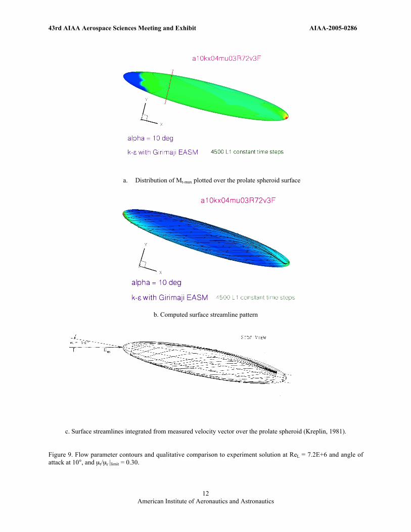
Two flow parameters will be examined next to provide a broader view of the solution characteristics and theircomparisons to the available experimental data: the maximum values of the turbulence Mach number, Mt-max andsurface streamline traces. In Figs. 8-11, the numerical and color range for the contours remains the same as shownin Fig. 7. Figure 8 shows a set of the distribution of these parameters on the surface of the spheroid for the case ofReL = 7.2E+6 at 30° incline. The experimentally measured transition zone, as implied by the abrupt jump in shearstress magnitude, is sketched into the figure as a band defined by two curves. The computed transition occurs earliertowards the nose than the measured shear stress jump. However, the downstream pattern agreement is quite good.The bottom parts of Fig. 8 show a comparison between the measured and the computed surface streamline traces.The computed streamline pattern on the upper body of the spheroid shows a weaker separation pattern than themeasurement. The measured separation starts near x/L = 0.20, while the computed separation pattern does not startuntil near x/L=0.60 at best. Figure 9 shows the comparison for the case of ReL = 7.2E+6 at 10° incline. Again, thecomputed transition occurred earlier towards the front of the spheroid by comparing the transition as indicated bythe computed Mt-max contours and the approximate location of the measured transition as indicated by the straightdash line across the spheroid in Fig. 8. The encouraging message, however, is that the computation automaticallyadjusted to a completely different transition pattern with fixed turbulence model parameters.

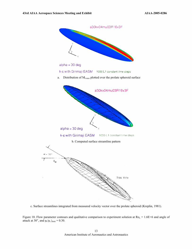
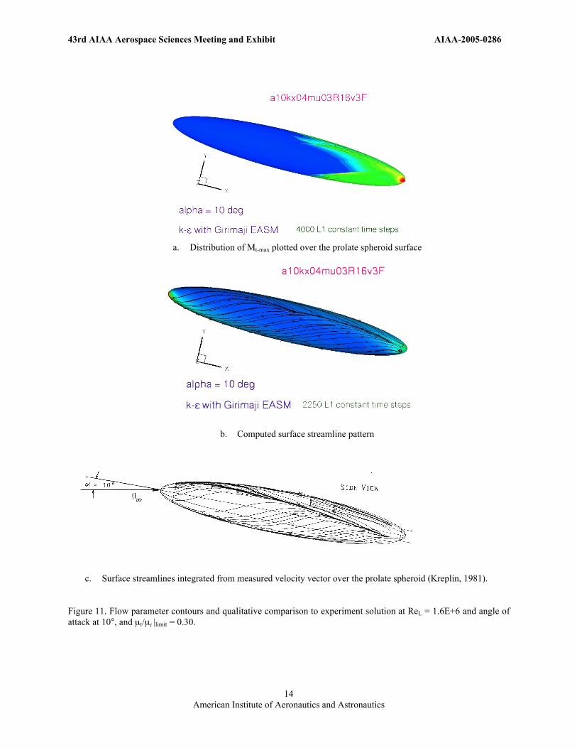
Figures 10 and 11 show the results for the lower Reynolds number cases, ReL = 1.6E+6. In Fig. 10 for the 30°incline, the computed boundary layer remained laminar over the entire spheroid according to the Mt-max magnitudeand the smoothness of the streamline pattern over the spheroid. The higher Mt-max values in the contour plot weredetermined to be a result of flow separation. In Fig. 11, the boundary layer over the upstream half the spheroidremained laminar, while the downstream half of the body was covered by a combination of flow separation andturbulent boundary layer. The indication of transition from a laminar to a turbulent boundary layer can be inferredthrough a combination of Mt-max distribution and the streamline pattern shown in Fig. 11. The magnitude of Mt-max

indicated that the boundary layer over the leading half of the spheroid was laminar. The flow separation line in thestreamline plot went smoothly in one direction. Near mid-body, however, a kink appeared along the separation lineand the flow separation boundary shifted towards the leeward side of the body. This was a typical flow behaviorindicating flow transition because flow separation was delayed on account of the boundary layer had becometurbulent. The report by Kreplin et al. stated that the boundary layer over the entire body was laminar. This was alsoillustrated by measured separation line which remained straight along the entire body length. It is interesting to notethat the measured flow separation line pattern showed a kink near the end of the spheroid. Such a kink did notappear in the other three measured streamline patterns by Kreplin et al.8. However, the original authors did notcomment on this particular feature in their measurement. The significance of such a kink in the data remainsunknown. Again, the encouraging message is that without changing the turbulence model limiters in the PAB3Dcode, the computations predicted laminar flow over most or all parts of the surface with a reduction of the Reynoldsnumber in accordance with the experimental measurements. Finally, it was observed that, consistent with the flatplate, transition was predicted early when compared to experimental data.



IV. Summary and Concluding RemarksA preliminary study of natural flow transition mimicking using simple two- and three-dimensional configurationshave led us to believe that a Navier-Stokes code such as the PAB3D code with a standard k-ε turbulence model anda theoretically based explicit algebraic stresses model (by Girimaji) have the sensitivity to mimic laminar toturbulent flow transition in the boundary layer. For the two-dimensional flat plate case, the results havequantitatively demonstrated that the computed flow transition Reynolds number has a consistent parametricrelationship to the inflow background turbulence intensity. A linear curve was fitted through the computed pointson a double logarithmic plot to represent the trend of variation as a power law between the background turbulenceintensity and the transition Reynolds number based on the transition point distance from the flat plate leading edge.The trend is qualitatively consistent with the empirical rules established for wind tunnel measurements and theclassical flat plate laminar to turbulent flow transition data obtained by Schubauer and Skramstad. In the three-dimensional prolate spheroid computations, a complex set of flow physics issues, such as pressure gradient, crossflow streamline curvatures, compressibility effects, vorticity, and shear flow stresses came into the picture. Thequantitative relationship between any of these effects and transition are recognized to be important, but has not yetbeen well established in the literature. Nevertheless, the 6:1 prolate spheroid flow simulation was completed for twoReynolds numbers at two angles of attack for comparison to existing data. The computed flow was found to mimictransition without specific input such as tripping, and comparisons with data showed interesting similarities in termsof flow transition characteristics. Although these computational investigations are preliminary and the comparisonto data is qualitative in nature, the positive indications are very encouraging for further studies of natural flowtransition mimicking using a standard Navier-Stokes solver, turbulence model, and an appropriate turbulent stressesmodel, preferably with a traceable theoretical basis. The authors certainly would hope that this limited study wouldgenerate interest in further theoretical and numerical research for this important subject in applied aerodynamics.

References

1Abdol-Hamid, Khaled S., Massey, Steven J., and Elmiligui, Alaa, “PAB3D Code Manual”, Cooperative development by theConfiguration Aerodynamics Branch, NASA Langley Research Center and Analytical Services & Materials, Inc. Hampton, VA.

2U !e !n !i !s !h !i !, ! !K !. ! !a !n !d ! !A !b !d !o !l !- !H !a !m !i !d !, ! !K !. !: ! !A ! !T !h !r !e !e !- !D !i !m !e !n !s !i !o !n !a !l ! !U !p !w !i !n !d !i !n !g ! !N !a !v !i !e !r !- !S !t !o !k !e !s ! !C !o !d !e ! !w !i !t !h ! !k !-ε ! !M !o !d !e !l ! ! !f !o !r ! !S !u !p !e !r !s !o !n !i !c !!F!l!o!w!s!"!,! !A!I!A!A! !2!2!n!d! !F!l!u!i!d! !a!n!d! !P!l!a!s!m!a!d!y!n!a!m!i!c! !C!o!n!f!e!r!e!n!c!e!,! !A!I!A!A! !9!1!-!1!6!6!9!,! !J!u!n!e! !1!9!9!1!.!

3Abdol-Hamid, K. S.: Implementation of Algebraic Stress Models in a General 3-D Navier-Stokes Method (PAB3D). NASACR-4702, December 1995.

4Carlson, J. R.: “Applications of algebraic Reynolds stress turbulence models – Part I.: Incompressible flat plate”, J.Propulsion and Power, 13 -5, 610-619, October 1997.

5Wilcox, David C.: Turbulence Modeling for CFD, pp.193-201, Second Ed., DCW Industries, 1998.6KrepIin, H.-P., Vollmers, H., and Meier, H. U.: "Wall shear stress measurements on an inclined prolate spheroid in the

DFVLR 3m x 3m Low Speed Wind Tunnel," Data Report, DFVLR IB 222-84/A 33, Gottingen, Germany., 1985.7Vollmers, H., Kreplin, H.-P., Meier, H. U., and Kiihn, A.: "Measured mean velocity field around a 1:6 prolate spheroid at

various cross sections," Data Report, DFVLR IB 221-85 A 08, Gottingen, Germany, 1985.8Kreplin, H.-P., Vollmers, H., Meier, H. U.: “Experimental determination of wall shear stress vectors on an inclined prolate

spheroid”, DFVLR-AVA, Gottingen, AFFDL-TR-80-3038, 1980.9Rodi, W.: “Experience with two-layer models combining the k-epsilon model with a one-equation model near the wall”,

AIAA Paper 91-0216, January 1991.10Warren, E. S., and Hassan, H. A.: “Transition closure model for predicting transition onset”, J. Aircraft, 35–5, September

1998.11Schubauer, G. B., Skramstad, H. K.: “Laminar boundary layer oscillations and transition on a flat plate”, NACA TR-909,

April 1943.12Schubauer, G. B., Klebanoff, P. S.: “Contributions to the mechanics of boundary layer transition”, NACA-TR-1289,

February 1955.13Craft, T. J., Launder, B. E., and Suga, K.: “Prediction of turbulent transitional phenomena with a nonlinear eddy-viscosity

model”, J. Heat and Fluid Flow, 18, pp. 15-28, 1997.14Chen, W. L., Lien, F. S., and Leschziner, M. A.: ”Non-linear eddy-viscosity modeling of transitional boundary layers

pertinent to turbomachine aerodynamics”, J. Heat and Fluid Flow, 19, 297-306, 1998.



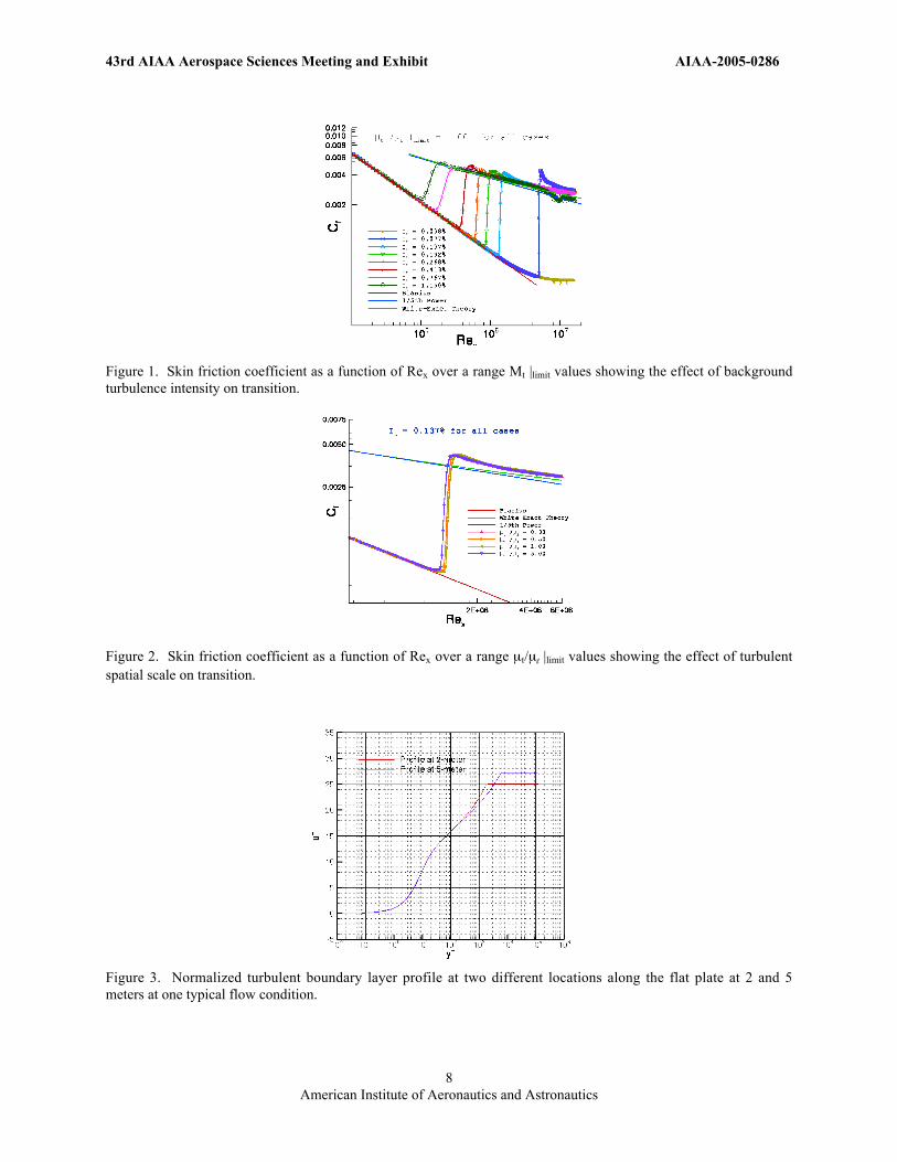
Figure 1. Skin friction coefficient as a function of Rex over a range Mt |limit values showing the effect of backgroundturbulence intensity on transition.

Figure 2. Skin friction coefficient as a function of Rex over a range µt/µl |limit values showing the effect of turbulentspatial scale on transition.

Figure 3. Normalized turbulent boundary layer profile at two different locations along the flat plate at 2 and 5meters at one typical flow condition.



Figure 4. Power law dependence between freestream turbulence intensity and transition Reynolds number based ondistance from the flat plate leading edge.

Figure 5. An exploratory study of the influence of decaying freestream turbulence intensity on transition Reynoldsnumber.

Figure 6. The 6:1 aspect ratio prolate magnified detail near the end and near-field grid topology.



a. µt/µl |limit = 0.10 b. µt/µl |limit = 0.20

c. µt/µl |limit = 0.30 d. µt/µl |limit = 0.40

Figure 7. The effect of µt/µl |limit on the computed laminar to turbulent flow transition, as indicated by the maximumturbulence Mach number distribution over the body surface, at ReL = 7.2E+6 and angle of attack at 30°.



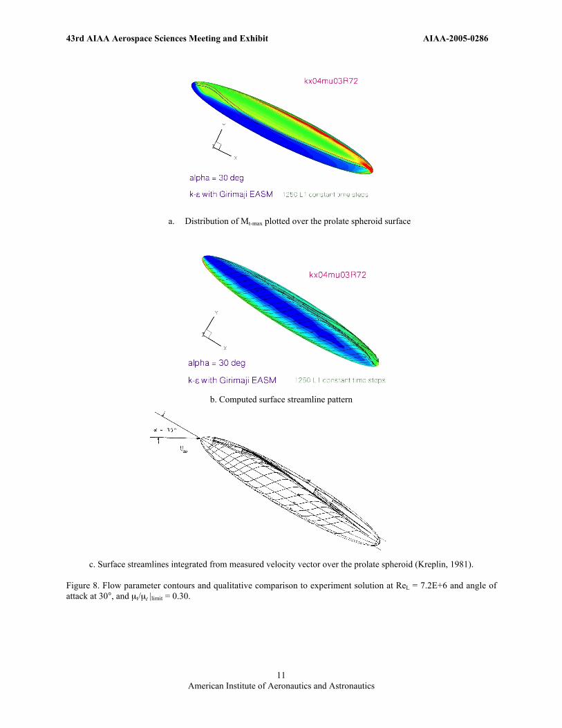
a. Distribution of Mt-max plotted over the prolate spheroid surface

b. Computed surface streamline pattern

c. Surface streamlines integrated from measured velocity vector over the prolate spheroid (Kreplin, 1981).

Figure 8. Flow parameter contours and qualitative comparison to experiment solution at ReL = 7.2E+6 and angle ofattack at 30°, and µt/µl |limit = 0.30.

mimicking natural laminar to turbulent flow … aiaa aerospace sciences meeting and exhibit...

Documents