Earth Syst. Dynam., 10, 347–364, 2019https://doi.org/10.5194/esd-10-347-2019© Author(s) 2019. This work is distributed underthe Creative Commons Attribution 4.0 License.

Millennium-length precipitation reconstruction oversouth-eastern Asia: a pseudo-proxy approach

Stefanie Talento1,2, Lea Schneider1, Johannes Werner4, and Jürg Luterbacher1,3

1Department of Geography, Climatology, Climate Dynamics and Climate Change,Justus Liebig University of Giessen, Giessen, Germany

2Physics Institute, Science Faculty, Universidad de la República, Montevideo, Uruguay3Center of International Development and Environmental Research,

Justus Liebig University of Giessen, Giessen, Germany4independent researcher

Correspondence: Stefanie Talento (stefanie.talento@geogr.uni-giessen.de)

Received: 24 January 2019 – Discussion started: 14 February 2019Accepted: 19 May 2019 – Published: 27 June 2019

Abstract. Quantifying precipitation variability beyond the instrumental period is essential for putting currentand future fluctuations into long-term perspective and providing a test bed for evaluating climate simulations. Forsouth-eastern Asia such quantifications are scarce and millennium-long attempts are still missing. In this studywe take a pseudo-proxy approach to evaluate the potential for generating summer precipitation reconstructionsover south-eastern Asia during the past millennium. The ability of a series of novel Bayesian approaches togenerate reconstructions at either annual or decadal resolutions and under diverse scenarios of pseudo-proxyrecords’ noise is analysed and compared to the classic analogue method.

We find that for all the algorithms and resolutions a high density of pseudo-proxy information is a neces-sary but not sufficient condition for a successful reconstruction. Among the selected algorithms, the Bayesiantechniques perform generally better than the analogue method, the difference in abilities being highest over thesemi-arid areas and in the decadal-resolution framework. The superiority of the Bayesian schemes indicates thatdirectly modelling the space and time precipitation field variability is more appropriate than just relying on a poolof observational-based analogues in which certain precipitation regimes might be absent. Using a pseudo-proxynetwork with locations and noise levels similar to the ones found in the real world, we conclude that perform-ing a millennium-long precipitation reconstruction over south-eastern Asia is feasible as the Bayesian schemesprovide skilful results over most of the target area.

1 Introduction

Earth’s climate varies in all spatial and temporal timescales,as it is forced by either natural or anthropic factors. To un-derstand the dynamics of such variability, the analysis of theavailable instrumental information is an essential tool. How-ever, the time coverage of the instrumental records is rathershort and, therefore, information from climate archives (nat-ural and documentary) going back centuries is important toput current and future changes into a long-term perspectiveand to serve as a validation terrain for model simulations with

the ultimate goal of understanding the underlying physicalmechanisms.

South-eastern Asian societies and economies are heavilydependent on the summer rainfall (monsoon-dominated) as afreshwater resource; thus, it is important to investigate howthese precipitation patterns have varied in the past to providea useful guide for the climate response to future changes. Pre-vious hydro climate field reconstructions (CFRs) over Asiarevealed a substantial mismatch between modelled and re-constructed precipitation patterns (Shi et al., 2017) and thespatial variability of large-scale droughts during the Little

Published by Copernicus Publications on behalf of the European Geosciences Union.

348 S. Talento et al.: Precipitation reconstruction over south-eastern Asia

Ice Age (Cook et al., 2010; S. Feng et al., 2013). Whilethese studies covered the last 500–700 years, a gridded hy-droclimate product going beyond Medieval times at a spatio-temporal high resolution is still missing. Whether such a longand highly resolved reconstruction is possible given data andmethodologies available nowadays is the subject of this pa-per.

Reconstructing the temporal evolution of climatic vari-ables in the space domain (CFR) based on the informationfrom a sparse network of proxies and partially overlappinginstrumental data is a complex mathematical problem. Firstof all, the proxy data used for generating reconstructions dis-play a set of characteristics that make their use challenging:their distribution in space and time is heterogeneous withfewer records further back in time; different proxy archiveshave different temporal resolutions and possibly include dat-ing uncertainties; proxy data might reflect different climatevariables (temperature, precipitation, sea-level changes, pH,seawater temperature, water mass circulation, etc.), record-ing climate conditions at different times of the year, and thesedata contain non-climatic information (usually referred to asnon-climatic noise). Second, the overlap with instrumentalobservations is commonly short, limiting opportunities forstatistical learning and further validation. Third, and in con-trast to average climate reconstructions, CFRs require thespatial scale-up of the available information, therefore im-plying the need for strategic inferring of the missing valuesin the target climate field, even in locations where no datamight be input. Finally, as the amount of paleoclimatic infor-mation becomes smaller back in time, it is virtually impos-sible to have an independent proxy data set to properly vali-date the output reconstruction. A common approach to over-come this shortcoming and have a proper validation stage isto use a pseudo-reality. The process of using a global climatemodel (GCM) simulation to assess the ability of a reconstruc-tion technique is known as a pseudo-proxy experiment (PPE;Smerdon, 2012; Mann and Rutherford, 2002). In a PPE, sim-ulated data are modified to mimic real-world proxies andinstrumental observations (called pseudo-proxy and pseudo-instrumental data sets), and the reconstruction algorithms areapplied. The reconstruction results are then compared withthe available simulated target field, giving an estimation ofthe skill of the method in real-world applications.

There are several ways to perform a CFR (see Luterbacherand Zorita, 2018, for a review). The classical approach isthrough a multivariate regression perspective: a statistical re-lationship between proxy and instrumental data is inferredfrom the overlapping (calibration) period and then, assum-ing stationarity of this relationship, the missing instrumen-tal values are predicted or reconstructed back through time.Some of the most common techniques for climate reconstruc-tions included in this category are regularised expectation–maximisation (RegEM, Schneider, 2001), canonical correla-tion analysis (CCA; Smerdon et al., 2010), Markov randomfields (Guillot et al., 2015) and the analogue method (Franke

et al., 2011). The performance of these methods strongly de-pends on the length of the instrumental data. If the overlap-ping period between proxy and instrumental data is short, incomparison with the number of spatial locations considered,the estimation of the covariance matrix is uncertain and thematrix inversion process is numerically unstable, leading topoor performance when presented with new data out of thelearning sample.

Another strategy to perform a CFR, more novel as ithas only recently been applied in paleoclimatology, is theBayesian approach (e.g. Tingley and Huybers, 2010, 2013;Werner et al., 2013, 2018; Luterbacher et al., 2016; Zhanget al., 2018). The Bayesian strategy is probabilistic, incorpo-rates information about the climate–proxy connection as con-straints on the reconstruction problem and has the benefit ofproviding more comprehensive uncertainty estimates for thederived reconstructions. Robust comparisons between estab-lished methods and the emerging efforts (Werner et al., 2013;Nilsen et al., 2018) underpin the benefits and justify furtherapplication of the computationally more expensive method.So far, most of the paleoclimatic applications of this method-ology involve temperature reconstructions. Efforts to applythis probabilistic framework to the more complex and highlyvariable hydroclimate are only in the initial stages, but the ad-vantages of the methodology over more classical approachesare auspicious.

Gómez-Navarro et al. (2015) used a PPE approach to as-sess the skill of several statistical techniques (classical re-gression methods and Bayesian) in reconstructing the pre-cipitation of the past 2 millennia over continental Europe.The authors find that none of the schemes shows better per-formance than the others and that precipitation reconstruc-tions over Europe are only possible given a spatially denseand uniformly distributed network of proxies, as the accu-racy strongly deteriorates with distance to the proxy sites.

In this study we propose to evaluate, via PPE, the poten-tial to generate a last-millennium summer precipitation re-construction for south-eastern Asia. We use three CFR tech-niques: Bayesian hierarchical modelling (BHM), BHM cou-pled with clustering processes (with two different numbers ofclusters), and the analogue method. For each of the schemeswe perform two reconstructions: one at annual and one atdecadal resolution. In addition, the influence of the noiselevel in pseudo-proxies on the final reconstruction is eval-uated.

This is the first time that a BHM approach is applied tothe hydroclimate of Asia, and its coupling with clusteringtechniques is a methodological advance, configuring an in-novation in the field. The systematic evaluation of the skillof these probabilistic methods, and the comparison with themore classical and well-established analogue technique, is anecessary step to learning about the precipitation variabil-ity and the opportunities for or obstacles to generating long-range informed guesses about it. The PPE exercise is a fun-damental validation step, essential for selecting the most ap-

Earth Syst. Dynam., 10, 347–364, 2019 www.earth-syst-dynam.net/10/347/2019/

S. Talento et al.: Precipitation reconstruction over south-eastern Asia 349

propriate method to improve real-world reconstructions and,finally, deriving a new and not previously attempted griddedproduct of south-eastern Asia summer precipitation duringthe last 1000 years. In this work only summer precipitationis targeted as the pseudo-proxy network selected is basedon real-world indicators of summer hydroclimatic variations(see Sect. 2.2).

The paper is organised as follows. In Sect. 2 we presentthe data and methodology and describe in detail the three re-construction techniques, as well as the skill scores used forquality evaluation. Section 3 is devoted to the results and dis-cussions: we evaluate the skill of each of the reconstructionmethods, at both annual and decadal resolution, and investi-gate the role of the pseudo-proxy noise. Finally, in Sect. 4 wepresent conclusions and a short outlook.

2 Data and methodology

2.1 Model

As a virtual reality setup for our study we use one full-forcing simulation (run 001) of the Community Earth Sys-tem Model (CESM) from the Last Millennium Ensemble(LME) project (Otto-Bliesner et al., 2016). The simulationis performed with a horizontal resolution of ∼ 2◦ (∼ 1◦) inthe atmosphere and land (ocean and ice) components. TheCESM is forced with reconstructions of the transient evolu-tion of solar intensity, volcanic emissions, greenhouse gases,aerosols, land use conditions and orbital parameters, all to-gether, for the period 850–2005. The target variable to re-construct is June–July–August (JJA) precipitation over conti-nental south-eastern Asia, here defined as all continental gridpoints in the domain Equator–50◦ N 72.5–127.5◦ E. Giventhe model resolution, this implies that the reconstruction isattempted over 366 grid points.

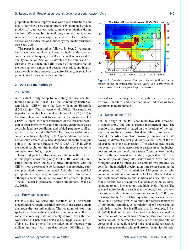
Figure 1 depicts the JJA mean precipitation in the run usedin this paper, considering only the last 100 years of simu-lation (period 1906–2005). Historical simulations with theCESM show a reasonable performance in reproducing sum-mer precipitation over continental Asia: the simulated JJAprecipitation is generally in agreement with observations,although a false rainfall centre over the eastern Qinghai–Tibetan Plateau is generated in these simulations (Wang etal., 2015).

2.2 Proxy data locations

For this study we select the locations of 47 real-worldprecipitation-/drought-sensitive proxies in the target domainthat span the last millennium. The locations of tree ring,speleothem, lake sediment and ice core sites as well as ofsome documentary data are mainly derived from the net-works used in Chen et al. (2015) and Ljungqvist et al. (2016)(Table 1). The criteria for the selection of records weremillennium-long (with start date before 1000 CE), at least

Figure 1. Simulated mean JJA precipitation (millimetres permonth) during the instrumental period (years 1906–2005) over con-tinental Asia. Black dots: pseudo-proxy network.

two values per century, terrestrial, published in the peer-reviewed literature, and described as an indicator of localvariations in hydroclimate.

2.3 Design of the PPEs

For the design of the PPEs we build two data networks:a pseudo-proxy one and a pseudo-instrumental one. Thepseudo-proxy network is based on the locations of the real-world hydroclimate proxies listed in Table 1. As some ofthese 47 records are in close proximity, this translates intohaving 38 different model grid points (about 10 % of the to-tal grid points in the study region). The selected locations arenot evenly distributed across south-eastern Asia: the highestconcentrations are found over eastern China and over the drylands in the north-west of the study region (Fig. 1). Thereare neither pseudo-proxy sites southward of 20◦ N nor overMongolia and the Himalayas. To emulate real proxies, weconsider the modelled precipitation time series spanning thecomplete period of the simulation (1156 years, either withannual or decadal resolution) at each of the 38 selected sitesand contaminate them by the addition of noise. We selectfour different levels of additive Gaussian white noise, corre-sponding to null, low, medium, and high levels of noise. Theselected noise levels are such that the correlations betweenthe original and contaminated time series are 1, 0.7, 0.5, and0.3, respectively. A correlation equal to 1 implies an idealisedsituation of perfect proxies to study the representativenessof our spatial sampling. A correlation of 0.7 represents anoptimistic situation, but is still realistic: for example, Shi etal. (2014) find correlations of up to 0.7 with a tree-based re-construction of the South Asian Summer Monsoon Index. Acorrelation of 0.5 between the proxy series and precipitationcorresponds to a medium-level noise, and could be regardedas the average situation with real proxies (examples for Asia:

www.earth-syst-dynam.net/10/347/2019/ Earth Syst. Dynam., 10, 347–364, 2019

350 S. Talento et al.: Precipitation reconstruction over south-eastern Asia

Table 1. List of the real-world proxy records used to select the locations of the pseudo-proxy network.

Site Longitude Latitude Archive Target season Reference

1 Anyemaqen Mountains 99.5 34.5 Tree Annual Gou et al. (2010)2 Balkhash Basin 75 46.9 Pollen Annual Z.-D. Feng et al. (2013)3 Buddha Cave 109.5 33.4 Speleothem Annual Paulsen et al. (2003)4 Central India Composite 82 19 Speleothem Summer Sinha et al. (2011)5 Delingha 97.38 37.38 Tree Annual Yang et al. (2014)6 Dharamjali Cave 80.21 29.52 Speleothem Annual Sanwal et al. (2013)7 Dongge Cave 108.8 25.28 Speleothem Annual Wang et al. (2005)8 Eastern Tibetan Plateau 102.52 32.77 Lake Annual Yu et al. (2006)9 Furong Cave 107.9 29.29 Speleothem Summer Li et al. (2011)10 Gonghai Lake 112.23 38.9 Lake Summer Liu et al. (2011)11 Great Bend of the Yellow River 115 35 Documentary Annual Gong and Hameed (1991)12 Guliya 81.48 35.28 Ice Annual Yao et al. (1996)13 Haihe River Basin 116 40 Documentary Annual Yan et al. (1993)14 Hani 126.51 42.21 Lake Annual Hong et al. (2005)15 Heihe River Basin 100 38.2 Tree Annual Yang et al. (2012)16 Heshang_Cave 109.36 19.41 Speleothem Annual Hu et al. (2008)17 Huangye Cave 105.12 33.92 Speleothem Annual Tan et al. (2011)18 Huguangyan Lakee 110.28 21.15 Lake Annual Zeng et al. (2012)19 Jianghuai 113.5 31.5 Documentary Annual Zheng et al. (2006)20 Jiangnan 115 30 Documentary Annual Zheng et al. (2006)21 Jiuxian Cave 109.1 33.57 Speleothem Summer Cai et al. (2010)22 Karakorum Mountains 74.93 35.9 Tree Annual Treydte et al. (2006)23 Kesang Cave 81.75 42.87 Speleothem Annual Zheng et al. (2012)24 Kusai Lake 93.25 35.4 Lake Summer Liu et al. (2009)25 Lake Aibi 82.84 44.9 Lake Annual Wang et al. (2013)26 Lake Gahai 102.33 34.24 Lake Annual He et al. (2013)27 Lake Hulun 117.5 49 Lake Annual Zhai et al. (2011)28 Lake Nam Co 90.78 30.73 Lake Summer Kasper et al. (2012)29 Lake Xiaolongwan 126.35 42.3 Lake Annual Chu et al. (2009)30 Lonxi Area 105 30 Documentary Annual Liangcheng Tan et al. (2008)31 North China Plains 115 38 Documentary Annual Zheng et al. (2006)32 North-eastern Tibetan Plateau 98 37 Tree Annual Yang et al. (2014)33 Qaidam Basin 97.5 37.2 Tree Annual Yin et al. (2008)34 Qaidam Basin 97.5 37.2 Tree Annual Wang et al. (2013)35 Qigai Nuur 109.5 39.5 Pollen Annual Sun and Feng (2013)36 Qilian Mountains 99.5 38.5 Tree Annual Zhang et al. (2011)37 Qinghai Province 99 37 Tree Annual Sheppard et al. (2004)38 Southern China 110 25 Documentary Annual Qian et al. (2003)39 Sugan Lake 93.9 38.85 Lake Annual He et al. (2013)40 Tsuifong Lake 121.6 24.5 Lake Annual Wang et al. (2013)41 Wanxiang Cave 105 33.19 Speleothem Annual Zhang et al. (2008)42 Wulungu Lake 87.15 47.15 Pollen Annual Liu et al. (2008)43 Yangtze Delta 121 32 Documentary Annual Zhang et al. (2008)44 Yangtze Delta 120 32 Documentary Annual Jiang et al. (2005)45 Yangtze Delta 115 30 Documentary Annual Qian et al. (2003)46 Yellow River 110 35 Documentary Annual Qian et al. (2003)47 Zhijin Cave 105.84 26.73 Speleothem Summer Kuo et al. (2011)

He et al., 2018; Liu et al., 2013). A correlation of 0.3 rep-resents a high-noise setting, which is still rather common inreal-world proxies (e.g. Jones et al., 2009).

For the pseudo-instrumental network we consider all thelocations for which a reconstruction is targeted: 366 modelgrid points in south-eastern Asia. For each of these locations,

we take the modelled precipitation time series for the last100 years of simulation (at either annual or decadal resolu-tion) and add a small Gaussian noise to represent the instru-mental errors present in real precipitation measurements. Theadded noise is such that, at each location, the correlation be-tween the original and contaminated time series is 0.95.

Earth Syst. Dynam., 10, 347–364, 2019 www.earth-syst-dynam.net/10/347/2019/

S. Talento et al.: Precipitation reconstruction over south-eastern Asia 351

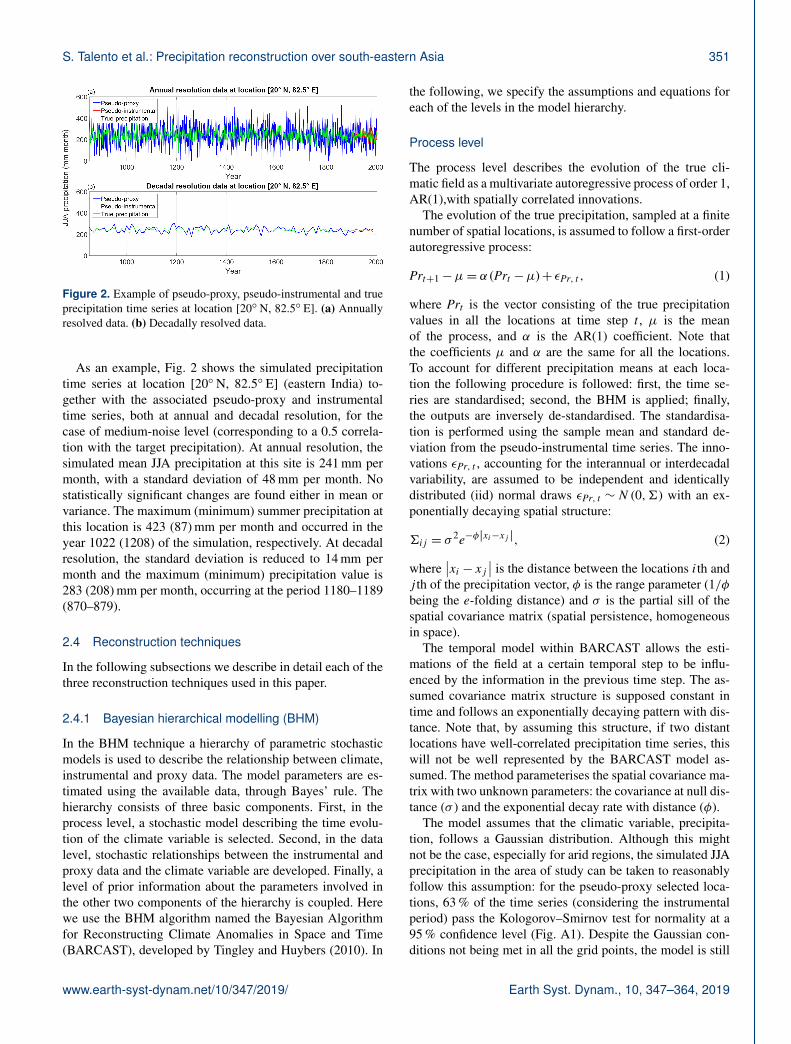
Figure 2. Example of pseudo-proxy, pseudo-instrumental and trueprecipitation time series at location [20◦ N, 82.5◦ E]. (a) Annuallyresolved data. (b) Decadally resolved data.

As an example, Fig. 2 shows the simulated precipitationtime series at location [20◦ N, 82.5◦ E] (eastern India) to-gether with the associated pseudo-proxy and instrumentaltime series, both at annual and decadal resolution, for thecase of medium-noise level (corresponding to a 0.5 correla-tion with the target precipitation). At annual resolution, thesimulated mean JJA precipitation at this site is 241 mm permonth, with a standard deviation of 48 mm per month. Nostatistically significant changes are found either in mean orvariance. The maximum (minimum) summer precipitation atthis location is 423 (87) mm per month and occurred in theyear 1022 (1208) of the simulation, respectively. At decadalresolution, the standard deviation is reduced to 14 mm permonth and the maximum (minimum) precipitation value is283 (208) mm per month, occurring at the period 1180–1189(870–879).

2.4 Reconstruction techniques

In the following subsections we describe in detail each of thethree reconstruction techniques used in this paper.

2.4.1 Bayesian hierarchical modelling (BHM)

In the BHM technique a hierarchy of parametric stochasticmodels is used to describe the relationship between climate,instrumental and proxy data. The model parameters are es-timated using the available data, through Bayes’ rule. Thehierarchy consists of three basic components. First, in theprocess level, a stochastic model describing the time evolu-tion of the climate variable is selected. Second, in the datalevel, stochastic relationships between the instrumental andproxy data and the climate variable are developed. Finally, alevel of prior information about the parameters involved inthe other two components of the hierarchy is coupled. Herewe use the BHM algorithm named the Bayesian Algorithmfor Reconstructing Climate Anomalies in Space and Time(BARCAST), developed by Tingley and Huybers (2010). In

the following, we specify the assumptions and equations foreach of the levels in the model hierarchy.

Process level

The process level describes the evolution of the true cli-matic field as a multivariate autoregressive process of order 1,AR(1),with spatially correlated innovations.

The evolution of the true precipitation, sampled at a finitenumber of spatial locations, is assumed to follow a first-orderautoregressive process:

Prt+1−µ= α (Prt −µ)+ εPr, t , (1)

where Prt is the vector consisting of the true precipitationvalues in all the locations at time step t , µ is the meanof the process, and α is the AR(1) coefficient. Note thatthe coefficients µ and α are the same for all the locations.To account for different precipitation means at each loca-tion the following procedure is followed: first, the time se-ries are standardised; second, the BHM is applied; finally,the outputs are inversely de-standardised. The standardisa-tion is performed using the sample mean and standard de-viation from the pseudo-instrumental time series. The inno-vations εPr, t , accounting for the interannual or interdecadalvariability, are assumed to be independent and identicallydistributed (iid) normal draws εPr, t ∼N (0,6) with an ex-ponentially decaying spatial structure:

6ij = σ2e−φ|xi−xj |, (2)

where∣∣xi − xj ∣∣ is the distance between the locations ith and

j th of the precipitation vector, φ is the range parameter (1/φbeing the e-folding distance) and σ is the partial sill of thespatial covariance matrix (spatial persistence, homogeneousin space).

The temporal model within BARCAST allows the esti-mations of the field at a certain temporal step to be influ-enced by the information in the previous time step. The as-sumed covariance matrix structure is supposed constant intime and follows an exponentially decaying pattern with dis-tance. Note that, by assuming this structure, if two distantlocations have well-correlated precipitation time series, thiswill not be well represented by the BARCAST model as-sumed. The method parameterises the spatial covariance ma-trix with two unknown parameters: the covariance at null dis-tance (σ ) and the exponential decay rate with distance (φ).

The model assumes that the climatic variable, precipita-tion, follows a Gaussian distribution. Although this mightnot be the case, especially for arid regions, the simulated JJAprecipitation in the area of study can be taken to reasonablyfollow this assumption: for the pseudo-proxy selected loca-tions, 63 % of the time series (considering the instrumentalperiod) pass the Kologorov–Smirnov test for normality at a95 % confidence level (Fig. A1). Despite the Gaussian con-ditions not being met in all the grid points, the model is still

www.earth-syst-dynam.net/10/347/2019/ Earth Syst. Dynam., 10, 347–364, 2019

352 S. Talento et al.: Precipitation reconstruction over south-eastern Asia

Figure 3. Correlation of simulated JJA precipitation time seriesacross different latitudinal bands versus distance. Only the instru-mental period (years 1906–2005) and the grid points in continentalAsia are considered for the calculation. (a) Annual-resolution data.(b) Decadal-resolution data. Dashed horizontal lines indicate thethresholds of statistical significance at a 95 % confidence level ac-cording to the Student’s t-test. For this plot, all grid points in thesame latitude band are grouped together and then one-to-one corre-lations are calculated between members of the same group.

valid, although it might not be the most optimal fit at theselocations.

Figure 3 shows the correlation decay with distance for thesimulated JJA precipitation for different latitudinal bands.For annual data (Fig. 3a), the correlation between precipi-tation time series in consecutive grid points is usually high,around 0.8. With few exceptions, the simulated precipitationfollows an exponentially decaying pattern with distance, withpoints located further away than 600 km showing no signifi-cant correlation. Therefore, we take the exponentially decay-ing spatial structure of the covariance matrix in BARCASTto be a reasonable assumption for the model. For decadal data(Fig. 3b), the correlation behaviours are not uniform with re-spect to the latitudinal bands. For some of the latitudes theplot follows an exponentially decaying shape, and for othersit additionally shows a teleconnection pattern (notably thenorthern-most 44–48◦ N latitude band).

Data level

The data level specifies the relationship between the mea-surements (both proxy and instrumental) and the true fieldvalues.

The instrumental observations at each time are assumed tobe noisy variations of the true precipitation field:

Instt =HInst, t(Prt + εInst, t

). (3)

The noise terms are assumed to be iid multivariate normaldraws εInst, t ∼N

(0,τ 2

Inst), while HInst, t is a diagonal matrix

with a 1 in position (i, i) if an instrumental observation isavailable at the ith location, and a 0 otherwise.

The proxy observations are assumed to follow an unknownstatistically linear relationship with the true precipitation ateach location:

Proxyt =HProxy, t(β1Proxyt +β0+ εProxy, t

). (4)

Again, the HProx, t is a diagonal matrix with ones only for thelocations with proxy observations, and the noise terms are iidnormal draws: εProxy, t ∼N

(0,τ 2

Proxy

).

Prior level

To close the scheme, prior distributions must be specified forthe eight scalar parameters

(α,µ,σ,φ,β1,β2,τ

2Inst,τ

2Proxy

)and the initial climate field (i.e. at the first time step). Weuse the same priors as Tingley and Huybers (2010) and se-lect prior distributions that are sufficiently diffuse to not haveany important influence on the posterior distributions.

Using Bayes’ rule the posterior distribution of each of theunknown variables can be calculated. Samples are drawnfrom these posterior distributions using a Gibbs sampler,with a Metropolis step (Gelman et al., 2003) to update φ,the spatial range parameter. The output of the Bayesian al-gorithm is not a unique reconstruction, but an ensemble of1200 equally probable draws, all of them consistent with themodel equations.

2.4.2 Bayesian hierarchical modelling coupled toclustering

Here we propose to couple the BHM with a clustering algo-rithm. The aim of the clustering step is to segregate south-eastern Asia into several clusters, according to similaritiesin the precipitation regimes during the pseudo-instrumentalperiod. After the clustering, the BHM code is run withineach cluster in an independent manner. Finally, all the resultsare merged together to produce the entire spatial reconstruc-tion over the post-850 period. The idea behind the clusteringstep is to reduce the complexity of the problem to be pre-sented to the BHM algorithm, as after clustering the codedoes not have to deal with extreme differences in precipita-tion regimes (as dipole patterns at mountain ranges) and alarge number of grid cells.

Earth Syst. Dynam., 10, 347–364, 2019 www.earth-syst-dynam.net/10/347/2019/

S. Talento et al.: Precipitation reconstruction over south-eastern Asia 353

We use a hierarchical agglomerative clustering technique.Each observation starts in its own cluster and pairs of clustersare agglomerated as one moves up in the hierarchy (Izenman,2008). We select a complete-linking strategy: the distancebetween sets of observations is defined as the maximum ofthe pairwise distances between the observations in each ofthe sets. First, the method groups together the two closestobservations, according to the selected distance, creating acluster of two observations. Then, the sets whose distance isminimum are agglomerated together, iteratively repeating theprocess.

Here, the elements to cluster together are the differentgrid points in south-eastern Asia. The input variables for themethod are the pseudo-instrumental precipitation time se-ries at each of these locations. The distance between twopoints is defined as 1 minus the correlation between thepseudo-instrumental precipitation time series at these loca-tions (points highly correlated display a small distance). Inthis way, the method groups together points whose pseudo-instrumental precipitation time series are highly correlated.We should note that the clustering algorithm does not requireany expert knowledge as it is a fully unsupervised machinelearning technique. This characteristic makes it easy to applyas a pre-BHM stage in any other context or area of study.

For both the annual and decadal reconstructions we selecttwo cases: clustering into 5 and into 10 groups (note that theclusters might be different when using the annual/decadal in-formation; see Fig. A2). We term the reconstructions in thiscategory BHM+5Clusters and BHM+10Clusters. The cri-teria for the selection of the number of clusters were thatmost of the clusters should include pseudo-proxy locations(if a cluster does not include pseudo-proxy information, theBHM scheme only uses instrumental-period data). While thiscondition is met without problems for 5 clusters, with the 10-cluster division (in both the annual and decadal cases), oneof the clusters is disjunct with the pseudo-proxy network. Asa consequence, a higher number of clustering divisions wasnot attempted.

2.4.3 Analogue method

The analogue method is a learning technique first introducedby Lorenz (1969) for weather forecasting. The techniqueuses predictors to determine the value of the target variable,based on the statistical relationship between them in a learn-ing set: the so-called pool of possible analogues. The methodcan also be applied to produce a CFR. In our study and foreach time step (year or decade), the predictor variables arethe proxy records (38 predictors) and the target variable isthe complete precipitation field at the given time step. Forthe annually resolved reconstruction the learning set consistsof the precipitation fields at each of the years in the instru-mental period, i.e. all the time steps in which we simulta-neously have the information about proxy and target. For thedecadally resolved reconstruction, the learning set consists of

the mean precipitation field in each possible 10-year periodduring the instrumental era.

The reconstruction of the precipitation field at time step tis obtained as follows. First, a distance between time stepsis defined. Let ti be a time step included in the pool (instru-mental period). Then, the distance between t and ti is, in thispaper, defined as the Euclidean distance between the vectorsof proxy data at times t and ti :

d (t, ti)=

√√√√ K∑j=1

(Prox

(lj , t

)−Prox

(lj , ti

))2, (5)

where Prox(lj , t

)is the value of the proxy at location lj and

time t . Locations l1, . . ., lK are all the proxy locations (K =38). Second, the time steps in the pool are ordered accordingto their distance from t . Third, the N closest time steps areselected from the pool and are termed analogues: t1, . . ., tN .Finally, the precipitation reconstruction for time t is the meanof the precipitation field in the N analogues:

Reconstruction(t)=Pr (t1)+ . . .+Pr (tN )

N. (6)

N can be any value between 1 and the total number of ele-ments in the pool of analogues. On the one hand, for annual(decadal) reconstructions, using N = 1 will imply having areconstruction identical to just 1 year (10-year mean) of theinstrumental period and, therefore, particularities of this year(10-year period) might be involved. On the other hand, us-ing the maximal N implies just giving as reconstruction themean during the instrumental period, which eliminates all theinter-annual or inter-decadal variability. In this paper we se-lect as N intermediate values, considering N approximatelyequal to 20 % of the number of possible analogues. Experi-ments using values ofN between 15 % and 40 % of the num-ber of possible analogues were performed and the results arenot significantly different to the ones selected to be displayedhere (not shown).

Note that in this paper we use the analogue method in itsclassical version (obtaining the pool of analogues from theobservational data set) and not in combination with the useof a GCM to draw the analogue cases from.

2.5 Skill metrics

To evaluate the performance of the CFR methodologies, wecompare the reconstruction with the true precipitation field.We select three different skill metrics. The first skill metric,the correlation coefficient, evaluates the ability of the recon-struction to reproduce the temporal evolution of the target. Ateach grid point, we calculate the Pearson correlation betweenthe reconstruction and the true precipitation time series, con-sidering the whole reconstruction period. As for the Bayesianalgorithms, we have an ensemble of reconstructions: we firstcalculate the correlation of each of these ensembles with the

www.earth-syst-dynam.net/10/347/2019/ Earth Syst. Dynam., 10, 347–364, 2019

354 S. Talento et al.: Precipitation reconstruction over south-eastern Asia

true precipitation and, finally, we show the mean of these cor-relations.

The second skill metric quantifies the absolute biases ofthe reconstruction at each location. Instead of directly usingthe root mean squared error (RMSE), we compare the RMSEof the different reconstructions with the RMSE obtained withthe simplest possible reconstruction: using the climatologicalmean during the instrumental period. In reconstruction stud-ies, this is usually referred to as the reduction of error (RE,Cook et al., 1994) and is defined, at each location l, as

RE(l)= 1−

∑t

(Pr (l, t)−Reconstruction(l, t))2∑t

(Pr (l, t)−Climatology(l))2 , (7)

where Reconstruction (l, t) is the reconstruction being evalu-ated at location l and time step t and Climatology (l) is theclimatological mean at location l. The sum is done over allthe time steps within the reconstruction period. In this casefor the Bayesian techniques, and to simplify the interpreta-tion, we show this metric for the median reconstruction.

The last skill metric is especially designed to evaluateprobabilistic ensemble forecasts of continuous predictandsand is, therefore, particularly suitable for evaluating theBayesian schemes. We use the continuous ranked probabil-ity score (Hersbach, 2000; Wilks, 2011; Werner et al., 2018).The CRPS measures the difference between the accumulatedprobability density function and the step function that jumpsfrom 0 to 1 at the observed value:

CRPS=

∞∫−∞

(F (y)−F0 (y))2dy, (8)

F0 (y)=0, y < observed value,1, y ≥ observed value. (9)

It has a negative orientation, meaning smaller values arebetter. This metric can only be provided for the Bayesianschemes and not for the analogue reconstructions.

3 Results

In the following sub-sections we evaluate the ability of thedifferent reconstruction techniques. In Sect. 3.1 we select apseudo-proxy scenario with medium noise level (equivalentto a correlation with the target precipitation of 0.5) and eval-uate the reconstruction schemes. In Sect. 3.2, we assess theimpact of the noise in the pseudo-proxy time series on thequality of the reconstruction.

3.1 Evaluation of reconstruction techniques:medium-noise pseudo-proxy case

As measures of performance we present the three selectedskill metrics (see Sect. 2.5 for details), and in each case, weshow the results at annual and decadal resolutions.

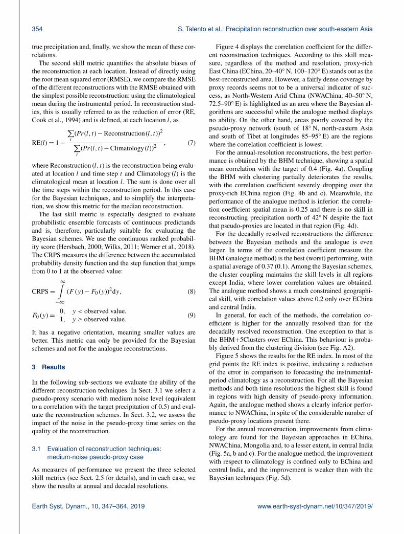
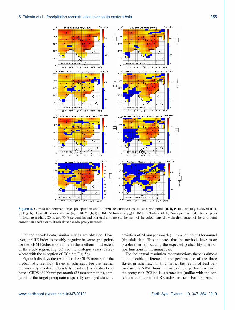
Figure 4 displays the correlation coefficient for the differ-ent reconstruction techniques. According to this skill mea-sure, regardless of the method and resolution, proxy-richEast China (EChina, 20–40◦ N, 100–120◦ E) stands out as thebest-reconstructed area. However, a fairly dense coverage byproxy records seems not to be a universal indicator of suc-cess, as North-Western Arid China (NWAChina, 40–50◦ N,72.5–90◦ E) is highlighted as an area where the Bayesian al-gorithms are successful while the analogue method displaysno ability. On the other hand, areas poorly covered by thepseudo-proxy network (south of 18◦ N, north-eastern Asiaand south of Tibet at longitudes 85–95◦ E) are the regionswhere the correlation coefficient is lowest.

For the annual-resolution reconstructions, the best perfor-mance is obtained by the BHM technique, showing a spatialmean correlation with the target of 0.4 (Fig. 4a). Couplingthe BHM with clustering partially deteriorates the results,with the correlation coefficient severely dropping over theproxy-rich EChina region (Fig. 4b and c). Meanwhile, theperformance of the analogue method is inferior: the correla-tion coefficient spatial mean is 0.25 and there is no skill inreconstructing precipitation north of 42◦ N despite the factthat pseudo-proxies are located in that region (Fig. 4d).

For the decadally resolved reconstructions the differencebetween the Bayesian methods and the analogue is evenlarger. In terms of the correlation coefficient measure theBHM (analogue method) is the best (worst) performing, witha spatial average of 0.37 (0.1). Among the Bayesian schemes,the cluster coupling maintains the skill levels in all regionsexcept India, where lower correlation values are obtained.The analogue method shows a much constrained geographi-cal skill, with correlation values above 0.2 only over EChinaand central India.

In general, for each of the methods, the correlation co-efficient is higher for the annually resolved than for thedecadally resolved reconstruction. One exception to that isthe BHM+5Clusters over EChina. This behaviour is proba-bly derived from the clustering division (see Fig. A2).

Figure 5 shows the results for the RE index. In most of thegrid points the RE index is positive, indicating a reductionof the error in comparison to forecasting the instrumental-period climatology as a reconstruction. For all the Bayesianmethods and both time resolutions the highest skill is foundin regions with high density of pseudo-proxy information.Again, the analogue method shows a clearly inferior perfor-mance to NWAChina, in spite of the considerable number ofpseudo-proxy locations present there.

For the annual reconstruction, improvements from clima-tology are found for the Bayesian approaches in EChina,NWAChina, Mongolia and, to a lesser extent, in central India(Fig. 5a, b and c). For the analogue method, the improvementwith respect to climatology is confined only to EChina andcentral India, and the improvement is weaker than with theBayesian techniques (Fig. 5d).

Earth Syst. Dynam., 10, 347–364, 2019 www.earth-syst-dynam.net/10/347/2019/

S. Talento et al.: Precipitation reconstruction over south-eastern Asia 355

Figure 4. Correlation between target precipitation and different reconstructions, at each grid point. (a, b, c, d) Annually resolved data.(e, f, g, h) Decadally resolved data. (a, e) BHM. (b, f) BHM+5Clusters. (c, g) BHM+10Clsuters. (d, h) Analogue method. The boxplots(indicating median, 25 %, and 75 % percentiles and non-outlier limits) to the right of the colour bars show the distribution of the grid-pointcorrelation coefficients. Black dots: pseudo-proxy network.

For the decadal data, similar results are obtained. How-ever, the RE index is notably negative in some grid pointsfor the BHM+5clusters (mainly in the northern-most extentof the study region; Fig. 5f) and the analogue cases (every-where with the exception of EChina; Fig. 5h).

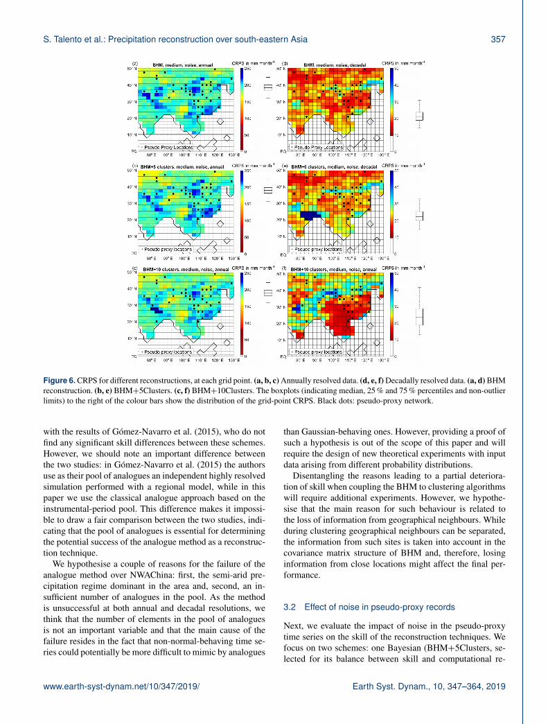
Figure 6 displays the results for the CRPS metric, for theprobabilistic methods (Bayesian schemes). For this metric,the annually resolved (decadally resolved) reconstructionshave a CRPS of 190 mm per month (22 mm per month), com-pared to the target precipitation spatially averaged standard

deviation of 34 mm per month (11 mm per month) for annual(decadal) data. This indicates that the methods have moreproblems in reproducing the expected probability distribu-tion functions in the annual case.

For the annual-resolution reconstructions there is almostno noticeable difference in the performance of the threeBayesian schemes. For this metric, the region of best per-formance is NWAChina. In this case, the performance overthe proxy-rich EChina is intermediate (unlike with the cor-relation coefficient and RE index metrics). For the decadal-

www.earth-syst-dynam.net/10/347/2019/ Earth Syst. Dynam., 10, 347–364, 2019

356 S. Talento et al.: Precipitation reconstruction over south-eastern Asia

Figure 5. RE index for different reconstructions, at each grid point. (a, b, c, d) Annually resolved data. (e, f, g, h) Decadally resolved data.(a, e) BHM. (b, f) BHM+5Clusters. (c, g) BHM+10Clsuters. (d, h) Analogue method. The boxplots (indicating median, 25 % and 75 %percentiles and non-outlier limits) to the right of the colour bars show the distribution of the grid-point RE index. Black dots: pseudo-proxynetwork.

resolution reconstructions, the performance among the meth-ods is quite different. While the spatial mean is in all threecases similar (around 22 mm per month), the spread amonggrid points is much higher for the BHM+10Clusters scheme.In particular, for the 10-cluster scheme the skill over Chinaand the south-east of the study region is much higher thanin the other methods. In general, the regions with a denseproxy network display better performance levels, and centralIndia and the north-east of the study area stand out as low-performing areas for all three methodologies.

Three main conclusions can be drawn from the experi-ments above: first, proxy-depleted areas cannot be success-fully reconstructed. Second, the Bayesian schemes are su-perior to the analogue method in all metrics (this differenceis particularly acute over NWAChina, where the analoguemethod fails despite the relatively good coverage by proxydata). Third, among the Bayesian algorithms the results aresimilar, although a partial deterioration of the skill is detectedin some regions when clustering is coupled.

The underperformance of the analogue method in com-parison with the BHM variants might seem in contradiction

Earth Syst. Dynam., 10, 347–364, 2019 www.earth-syst-dynam.net/10/347/2019/

S. Talento et al.: Precipitation reconstruction over south-eastern Asia 357

Figure 6. CRPS for different reconstructions, at each grid point. (a, b, c) Annually resolved data. (d, e, f) Decadally resolved data. (a, d) BHMreconstruction. (b, e) BHM+5Clusters. (c, f) BHM+10Clusters. The boxplots (indicating median, 25 % and 75 % percentiles and non-outlierlimits) to the right of the colour bars show the distribution of the grid-point CRPS. Black dots: pseudo-proxy network.

with the results of Gómez-Navarro et al. (2015), who do notfind any significant skill differences between these schemes.However, we should note an important difference betweenthe two studies: in Gómez-Navarro et al. (2015) the authorsuse as their pool of analogues an independent highly resolvedsimulation performed with a regional model, while in thispaper we use the classical analogue approach based on theinstrumental-period pool. This difference makes it impossi-ble to draw a fair comparison between the two studies, indi-cating that the pool of analogues is essential for determiningthe potential success of the analogue method as a reconstruc-tion technique.

We hypothesise a couple of reasons for the failure of theanalogue method over NWAChina: first, the semi-arid pre-cipitation regime dominant in the area and, second, an in-sufficient number of analogues in the pool. As the methodis unsuccessful at both annual and decadal resolutions, wethink that the number of elements in the pool of analoguesis not an important variable and that the main cause of thefailure resides in the fact that non-normal-behaving time se-ries could potentially be more difficult to mimic by analogues

than Gaussian-behaving ones. However, providing a proof ofsuch a hypothesis is out of the scope of this paper and willrequire the design of new theoretical experiments with inputdata arising from different probability distributions.

Disentangling the reasons leading to a partial deteriora-tion of skill when coupling the BHM to clustering algorithmswill require additional experiments. However, we hypothe-sise that the main reason for such behaviour is related tothe loss of information from geographical neighbours. Whileduring clustering geographical neighbours can be separated,the information from such sites is taken into account in thecovariance matrix structure of BHM and, therefore, losinginformation from close locations might affect the final per-formance.

3.2 Effect of noise in pseudo-proxy records

Next, we evaluate the impact of noise in the pseudo-proxytime series on the skill of the reconstruction techniques. Wefocus on two schemes: one Bayesian (BHM+5Clusters, se-lected for its balance between skill and computational re-

www.earth-syst-dynam.net/10/347/2019/ Earth Syst. Dynam., 10, 347–364, 2019

358 S. Talento et al.: Precipitation reconstruction over south-eastern Asia

Figure 7. Spatial mean correlation skill of reconstruction tech-niques for different noise levels (expressed here in terms of the cor-relation between the pseudo-proxy and truth).

quirements, as shown in Sect. 3.1) and the analogue method.We work with four noise levels for the pseudo-proxy timeseries: high noise (correlation with truth: 0.3), medium noise(correlation with truth: 0.5), low noise (correlation with truth:0.7) and perfect proxy (correlation with truth: 1). Note thatthe medium-noise proxy case corresponds to the level usedthrough Sect. 3.1. To simplify and summarise the results, inthis subsection we display the reconstruction performance interms of only one skill measure: the correlation coefficient.

Figure 7 shows the dependency of the correlation coef-ficient, averaged in space, with noise levels in the pseudo-proxy records. At annual resolution, the skill of the meth-ods increases in an almost linear way with the quality ofthe pseudo-proxy records, except for a drop in the Bayesianskill in the no-noise scenario. The BHM+5Clusters perfor-mance is better than the analogue method in all cases ex-cept the no-noise one. For high-noise proxies the skill ofthe BHM+5Clusters (analogue method) is 0.23 (0.18), whilein the perfect-proxy scenario the BHM+5Clusters (analoguemethod) reaches 0.30 (0.42). For decadally resolved recon-structions the picture is quite different. The Bayesian ap-proaches show a quasi-constant skill for the medium, low andno-noise examples (around 0.33) and the analogue methodperforms poorly, showing for all the noise types a skill be-tween 0.09 and 0.15. While for the Bayesian schemes thespatial average skill for the annual or decadal resolutions issimilar, the difference between annual versus decadal is im-portant in the analogue case. To complement the spatiallyaveraged information, Figs. 8 and 9 show the sensitivity ofthe correlation skill measure field to the noise levels in thepseudo-proxies for the BHM+5Clusters and the analoguemethod, respectively.

For the Bayesian algorithm (Fig. 8), the perfect-proxy caseshows high performance over NWAChina, EChina and north-east of the study area, at annual and decadal resolutions.For the annual reconstruction, the skill of the scheme is lowsouthward of 25◦ N and over some grid cells in the north

of the area. For the decadal reconstruction, the same areasare also problematic and, in addition, most of India is notwell reconstructed. In general, as the noise level in the inputpseudo-proxies increases, the performance of the method de-teriorates, and for the high-noise case only East China andthe north-west of the study region show moderate success.

Figure 9 presents the analogue method performance. Forannual resolution, in the case of perfect pseudo-proxies, themethod is successful in the central part of the study area (be-tween 15 and 45◦ N), while the northern and southern-mostextremes are not well reconstructed. However, the decadalcounterpart is only skilful in EChina. At the high-noise endof the spectrum, the analogue method only shows a satisfac-tory performance in EChina, between 20 and 40◦ N (between25 and 35◦ N) for the annually resolved (decadally resolved)reconstruction.

To summarise, as expected, the noise in the pseudo-proxytime series is important, as the quality of the reconstructionrapidly decreases with the noise level.

4 Summary and conclusions

This study evaluates the ability of several statistical tech-niques to reconstruct the precipitation field over south-eastern Asia in a PPE setting. The reconstructions are per-formed using 1156 years of model simulation (correspondingto the period 850–2005), at annual and decadal resolution.The techniques used are BHM, BHM coupled with cluster-ing (dividing south-eastern Asia into 5 or 10 clusters) and theanalogue method. While the analogue method is a classicalapproach and has been widely used, the Bayesian variants arenovel for the hydro-climatological reconstructions’ field, thisbeing the first time the technique is applied for Asian precipi-tation reconstruction. Moreover, the coupling of the Bayesianmodelling with clustering algorithms is also an innovationthat could potentially lead to a more widespread applicationof these computationally intensive processes.

We find that for all the algorithms and resolutions a highdensity of pseudo-proxy information is a necessary but notsufficient condition for a successful reconstruction. On theone hand, the lack of proxy data over regions such as thenorth-east of the study area, south of Tibet and south of20◦ N, determines that none of the methods is capable ofdelivering a skilful reconstruction. On the other hand, agood performance over the proxy-rich areas of EChina andNWAChina is not guaranteed just by the amount of datapresent there: while all the methods are highly successfulover EChina, only the Bayesian algorithms deliver qualityreconstructions over NWAChina.

Among the three Bayesian schemes the differences in skillare not extremely notorious, although a partial deteriora-tion of the skill is detected in some regions when cluster-ing is coupled. Noting that the Bayesian technique withoutany form of pre-clustering of the area of interest (BHM)

Earth Syst. Dynam., 10, 347–364, 2019 www.earth-syst-dynam.net/10/347/2019/

S. Talento et al.: Precipitation reconstruction over south-eastern Asia 359

Figure 8. BHM+5Clusters performance in terms of correlation with the target for different levels of noise at annual (a, b, c, d) ordecadal (e, f, g, h) resolution. (a, b) No noise. (c, d) Low noise. (e, f) Medium-level noise. (g, h) High noise. The boxplots (indicatingmedian, 25 % and 75 % percentiles and non-outlier limits) to the right of the colour bars show the distribution of the grid-point correlationcoefficients. Black dots: pseudo-proxy network.

is extremely computationally expensive, coupling it with aclustering scheme (BHM+5Clusters or BHM+10Clusters)seems to be a good compromise between success of thereconstruction and computational demand (with computingtimes reduced by up to 50 %).

We also find that the quality of the final reconstructionsis highly sensitive to the noise levels included in the inputpseudo-proxy data, those variables being negatively corre-lated. Only under a perfect-proxy (no-noise) scenario and atannual resolution is the analogue method capable of over-performing the Bayesian schemes over most areas. Even in

this ideal no-noise case NWAChina remains elusive for theanalogue methodology.

As a summary, we find that for millennium-length pre-cipitation reconstructions over south-eastern Asia a densenetwork of proxy information is mandatory for success,highlighting the complex nature of the precipitation fieldin the area of study. Among the selected algorithms, theBayesian techniques perform generally better than the ana-logue method, the difference in abilities being highest overthe semi-arid north-west and in the decadal-resolution frame-work. The superiority of the Bayesian approach indicates thatdirectly modelling the space and time precipitation field vari-

www.earth-syst-dynam.net/10/347/2019/ Earth Syst. Dynam., 10, 347–364, 2019

360 S. Talento et al.: Precipitation reconstruction over south-eastern Asia

Figure 9. Analogue method performance in terms of correlation with target for different levels of noise at annual (a, b, c, d) ordecadal (e, f, g, h) resolution. (a, b) No noise. (c, d) Low noise. (e, f) Medium-level noise. (g, h) High noise. The boxplots (indicatingmedian, 25 % and 75 % percentiles and non-outlier limits) to the right of the colour bars show the distribution of the grid-point correlationcoefficients. Black dots: pseudo-proxy network.

ability is more appropriate than just relying on similaritieswithin a restricted pool of observational analogues, in whichcertain regimes might not be present.

A natural next step is to implement real-world recon-structions of precipitation in the region of continental south-eastern Asia. These PPEs are auspicious for such a future en-deavour, as some moderate skill can be expected in most ofthe region. Nevertheless, it is important to acknowledge thatthese experiments are highly idealised and that real-worlddata might incorporate additional constraints and challenges.Additionally, more PPEs could also be designed by omit-ting some of the simplifications assumed here. For exam-

ple, while here we only took proxy time series that cover thewhole period of interest, with the same temporal resolution,same signal to noise relation and same relationship with theunderlying hydroclimatic variable of interest, some of theseconstraints could be modified to better resemble reality.

Data availability. Data sets, codes and analysisscripts used in this study can be obtained from:https://doi.org/10.17605/OSF.IO/B2RXP (Talento, 2019).

Earth Syst. Dynam., 10, 347–364, 2019 www.earth-syst-dynam.net/10/347/2019/

S. Talento et al.: Precipitation reconstruction over south-eastern Asia 361

Appendix A

Figure A1. Kolmogorov–Smirnov normality test on the simulated JJA precipitation during the instrumental period (years 1906–2005, atannual resolution). (a) Rejection or acceptance of the normality hypothesis, at a 95 % confidence level; (b) p values. Black dots: pseudo-proxy network.

Figure A2. Divisions into clusters (in each plot different colors indicate different clusters), using the simulated JJA precipitation in theinstrumental period (years 1996–2005) as input. (a) Annual data, division into 5 clusters, (b) annual data, division into 10 clusters, (c) decadaldata, division into 5 clusters, and (d) decadal data, division into 10 clusters. Magenta dots: pseudo-proxy network.

www.earth-syst-dynam.net/10/347/2019/ Earth Syst. Dynam., 10, 347–364, 2019

362 S. Talento et al.: Precipitation reconstruction over south-eastern Asia

Author contributions. ST made all the calculations, produced allthe figures and wrote the main text. LS, JW and JL contributed withdiscussions and comments on the manuscript.

Competing interests. The authors declare that they have no con-flict of interest.

Special issue statement. This article is part of the special issue“Hydro-climate dynamics, analytics and predictability”. It is not as-sociated with a conference.

Acknowledgements. Stefanie Talento, Lea Schneider and JürgLuterbacher are supported by the Belmont Forum and JPI-ClimateCollaborative Research Action “INTEGRATE: An integrated data-model study of interactions between tropical monsoons and ex-tratropical climate variability and extremes”. Jürg Luterbacher ac-knowledges support by the UK–China Research and InnovationPartnership Fund through the Met Office Climate Science for Ser-vice Partnership China (CSSP) as part of the Newton Fund.

The authors thank the reviewers for constructive criticism andsuggestions that improved the quality of the paper. The authors alsothank the proxy and model data providers.

Financial support. This research has been supported by theBelmont Forum, JPI-Climate (INTEGRATE grant).

This open-access publication was fundedby Justus Liebig University.

Review statement. This paper was edited by Naresh Devineniand reviewed by Tine Nilsen and one anonymous referee.

References

Cai, Y., Tan, L., Cheng, H., An, Z., Edwards, R. L.,Kelly, M. J., Kong, X., and Wang, X.: The variationof summer monsoon precipitation in central China sincethe last deglaciation, Earth Planet. Sc. Lett., 291, 21–31,https://doi.org/10.1016/j.epsl.2009.12.039, 2010.

Chen, J., Chen, F., Feng, S., Huang, W., Liu, J., and Zhou, A.:Hydroclimatic changes in China and surroundings during theMedieval Climate Anomaly and Little Ice Age: spatial patternsand possible mechanisms, Quaternary Sci. Rev., 107, 98–111,https://doi.org/10.1016/j.quascirev.2014.10.012, 2015.

Chu, G., Sun, Q., Wang, X., Li, D., Rioual, P., Qiang, L.,Han, J., and Liu, J.: A 1600 year multiproxy record of pa-leoclimatic change from varved sediments in Lake Xiaolong-wan, northeastern China, J. Geophys. Res., 114, D22108,https://doi.org/10.1029/2009JD012077, 2009.

Cook, E. R., Briffa, K. R., and Jones, P. D.: Spatial re-gression methods in dendroclimatology: a review and com-parison of two techniques, Int. J. Climatol., 14, 379–402,https://doi.org/10.1002/joc.3370140404, 1994.

Cook, E. R., Anchukaitis, K. J., Buckley, B. M., D’Arrigo, R. D.,Jacoby, G. C., and Wright, W. E. X.: Asian monsoon failure andmegadrought during the last millennium, Science, 328, 486–489,2010.

Feng, S., Hu, Q., Wu, Q., and Mann, M. E.: A gridded re-construction of warm season precipitation for Asia span-ning the past half millennium, J. Climate, 26, 2192–2204,https://doi.org/10.1175/JCLI-D-12-00099.1, 2013.

Feng, Z.-D., Wu, H. N., Zhang, C. J., Ran, M., and Sun, A. Z.:Bioclimatic change of the past 2500 years within the BalkhashBasin, eastern Kazakhstan, Central Asia, Quatern. Int., 311, 63–70, https://doi.org/10.1016/j.quaint.2013.06.032, 2013.

Franke, J., González-Rouco, J. F., Frank, D., and Graham, N. E.:200 years of European temperature variability: insights fromand tests of the proxy surrogate reconstruction analog method,Clim. Dynam., 37, 133–150, https://doi.org/10.1007/s00382-010-0802-6, 2011.

Gelman, A., Carlin, J., Stern, H., and Rubin, D.: Bayesian DataAnal, 3rd edn., Chapman and Hall, London, 2003.

Gómez-Navarro, J. J., Werner, J., Wagner, S., Luterbacher, J., andZorita, E.: Establishing the skill of climate field reconstruc-tion techniques for precipitation with pseudoproxy experiments,Clim. Dynam., 45, 1395–1413, https://doi.org/10.1007/s00382-014-2388-x, 2015.

Gong, G. and Hameed, S.: The variation of moisture conditions inChina during the last 2000 years, Int. J. Climatol., 11, 271–283,https://doi.org/10.1002/joc.3370110304, 1991.

Gou, X., Deng, Y., Chen, F., Yang, M., Fang, K., Gao, L., Yang,T., and Zhang, F.: Tree ring based streamflow reconstruction forthe Upper Yellow River over the past 1234 years, Chinese Sci.Bull., 55, 4179–418, https://doi.org/10.1007/s11434-010-4215-z, 2010.

Guillot, D., Rajaratnam, B., and Emile-Geay, J.: Statistical paleocli-mate reconstructions via Markov random fields, Ann. Appl. Stat.,9, 324–352, https://doi.org/10.1214/14-AOAS794, 2015.

He, M., Bräuning, A., Grießinger, J., Hochreuther, P., andWernicke, J.: May–June drought reconstruction over thepast 821 years on the south-central Tibetan Plateau derivedfrom tree-ring width series, Dendrochronologia, 47, 48–57,https://doi.org/10.1016/j.dendro.2017.12.006, 2018.

He, Y., Zhao, C., Wang, Z., Wang, H., Song, M., Liu, W., and Liu,Z.: Late Holocene coupled moisture and temperature changes onthe northern Tibetan Plateau, Quaternary Sci. Rev., 80, 47–57,https://doi.org/10.1016/j.quascirev.2013.08.017, 2013.

Hersbach, H.: Decomposition of the continuous ranked prob-ability score for ensemble prediction systems, WeatherForecast., 15, 559–570, https://doi.org/10.1175/1520-0434(2000)015<0559:DOTCRP>2.0.CO;2, 2000.

Hong, Y. T., Hong, B., Lin, Q. H., Shibata, Y., Hirota, M.,Zhu, Y. X., Leng, X. T., Wang, Y., Wang, H., and Yi, L.:Inverse phase oscillations between the East Asian and In-dian Ocean summer monsoons during the last 12000 yearsand paleo-El Niño, Earth Planet. Sc. Lett., 231, 337–346,https://doi.org/10.1016/j.epsl.2004.12.025, 2005.

Hu, C., Henderson, G. M., Huang, J., Xie, S., Sun, Y., and John-son, K. R.: Quantification of Holocene Asian monsoon rainfallfrom spatially separated cave records, Earth Planet. Sc. Lett.,266, 221–232, https://doi.org/10.1016/j.epsl.2007.10.015, 2008.

Earth Syst. Dynam., 10, 347–364, 2019 www.earth-syst-dynam.net/10/347/2019/

S. Talento et al.: Precipitation reconstruction over south-eastern Asia 363

Izenman, A. J.: Modern Multivariate Statistical Techniques,Springer Texts in Statistics, Springer-Verlag New York, 2008.

Jiang, T., Zhang, Q., Blender, R., and Fraedrich, K.: Yangtze Deltafloods and droughts of the last millennium: Abrupt changesand long term memory, Theor. Appl. Climatol., 82, 131–141,https://doi.org/10.1007/s00704-005-0125-4, 2005

Jones, P. D., Briffa, K. R., Osborn, T. J., Lough, J. M., van Om-men, T. D., Vinther, B. M., Luterbacher, J., Wahl, E., Zwiers,F. W., Schmidt, G. A., Ammann, C., Mann, M. E., Buck-ley, B. M., Cobb, K., Esper, J., Goosse, H., Graham, N.,Jansen, E., Kiefer, T., Kull, C., Küttel, M., Mosley-Thompson,E., Overpeck, J. T., Riedwyl, N., Schulz, M., Tudhope, S.,Villalba, R., Wanner, H., Wolff, E., and Xoplaki, E.: High-resolution palaeoclimatology of the last millennium: a reviewof current status and future prospects, Holocene, 19, 3–49,https://doi.org/10.1177/0959683608098952, 2009.

Kasper, T., Haberzettl, T., Doberschütz, S., Daut, G., Wang,J., Zhu, L., Nowaczyk, N., and Mäusbacher, R.: IndianOcean Summer Monsoon (IOSM)-dynamics within the past4 ka recorded in the sediments of Lake Nam Co, centralTibetan Plateau (China), Quaternary Sci. Rev., 39, 73–85,https://doi.org/10.1016/j.quascirev.2012.02.011, 2012.

Kuo, T. S., Liu, Z. Q., Li, H. C., Wan, N. J., Shen, C. C.,and Ku, T. L.: Climate and environmental changes during thepast millennium in central western Guizhou, China as recordedby Stalagmite ZJD-21, J. Asian Earth Sci., 40, 1111–1120,https://doi.org/10.1016/j.jseaes.2011.01.001, 2011.

Li, H. C., Lee, Z. H., Wan, N. J., Shen, C. C., Li, T. Y., Yuan, D.X., and Chen, Y. H.: The δ18O and δ13C records in an aragonitestalagmite from Furong Cave, Chongqing, China: A-2000-yearrecord of monsoonal climate, J. Asian Earth Sci., 40, 1121–1130,https://doi.org/10.1016/j.jseaes.2010.06.011, 2011.

Liangcheng, T., Yanjun, C., Liang, Y., Zhisheng, A., and Li, A.:Precipitation variations of Longxi, northeast margin of TibetanPlateau since AD 960 and their relationship with solar activ-ity, Clim. Past, 4, 19–28, https://doi.org/10.5194/cp-4-19-2008,2008.

Liu, J., Chen, F., Chen, J., Xia, D., Xu, Q., Wang, Z., and Li, Y.: Hu-mid medieval warm period recorded by magnetic characteristicsof sediments from Gonghai Lake, Shanxi, North China, ChineseSci. Bull., 56, 2464–2474, https://doi.org/10.1007/s11434-011-4592-y, 2011.

Liu, X., Herzschuh, U., Shen, J., Jiang, Q., and Xiao, X.: Holoceneenvironmental and climatic changes inferred from Wulungu Lakein northern Xinjiang, China, Quaternary Res., 70, 412–425,https://doi.org/10.1016/j.yqres.2008.06.005, 2008.

Liu, X., Dong, H., Yang, X., Herzschuh, U., Zhang, E., Stuut, J.-B. W., and Wang, Y.: Late Holocene forcing of the Asian winterand summer monsoon as evidenced by proxy records from thenorthern Qinghai–Tibetan Plateau, Earth Planet. Sc. Lett., 280,276–284, https://doi.org/10.1016/j.epsl.2009.01.041, 2009.

Liu, Z., Liu, Q., Torrent, J., Barrón, V., and Hu, P.: Test-ing the magnetic proxy χFD/HIRM for quantifying pa-leoprecipitation in modern soil profiles from ShaanxiProvince, China, Global Planet. Change, 110, 368–378,https://doi.org/10.1016/j.gloplacha.2013.04.013, 2013.

Ljungqvist, F. C., Krusic, P. J., Sundqvist, H. S., Zorita, E.,Brattström, G., and Frank, D.: Northern Hemisphere hydrocli-

mate variability over the past twelve centuries, Nature, 532, 94–98, https://doi.org/10.1038/nature17418, 2016.

Lorenz, E. N.: Atmospheric predictability as revealed by naturallyoccurring analogues, J. Atmos. Sci., 26, 636–646, 1969.

Luterbacher, J. and Zorita, E.: Spatial climate field reconstructions,in: The Palgrave Handbook of Climate History, edited by: White,S., Pfister, C., and Mauelshagen, F., Palgrave Macmillan, UK,131–139, 2018.

Luterbacher, J., Werner, J. P., Smerdon, J. E., et al.: European sum-mer temperatures since Roman times, Environ. Res. Lett., 11,024001, https://doi.org/10.1088/1748-9326/11/2/024001, 2016.

Mann, M. E. and Rutherford, S.: Climate reconstruction us-ing “Pseudoproxies”, Geophys. Res. Lett., 29, 139-1–139-4,https://doi.org/10.1029/2001GL014554, 2002.

Nilsen, T., Werner, J. P., Divine, D. V., and Rypdal, M.: Assessingthe performance of the BARCAST climate field reconstructiontechnique for a climate with long-range memory, Clim. Past, 14,947–967, https://doi.org/10.5194/cp-14-947-2018, 2018.

Otto-Bliesner, B. L., Brady, E. C., Fasullo, J., Jahn, A., Landrum, L.,Stevenson, S., Rosenbloom, N., Mai, A., and Strand, G.: Climatevariability and change since 850 CE: An ensemble approach withthe Community Earth System Model, B. Am. Meteorol. Soc., 97,735–754, https://doi.org/10.1175/BAMS-D-14-00233.1, 2016.

Paulsen, D. E., Li, H. C., and Ku, T. L.: Climate variabilityin central China over the last 1270 years revealed by high-resolution stalagmite records, Quaternary Sci. Rev., 22, 691–701,https://doi.org/10.1016/S0277-3791(02)00240-8, 2003.

Qian, W., Hu, Q., Zhu, Y., and Lee, D. K.: Centennial-scaledry-wet variations in East Asia, Clim. Dynam., 21, 77–89,https://doi.org/10.1007/s00382-003-0319-3, 2003.

Sanwal, J., Kotlia, B. S., Rajendran, C., Ahmad, S. M., Rajen-dran, K., and Sandiford, M.: Climatic variability in Central In-dian Himalaya during the last ∼ 1800 years: Evidence from ahigh resolution speleothem record, Quaternary Int., 304, 183–192, https://doi.org/10.1016/j.quaint.2013.03.029, 2013.

Schneider, T.: Analysis of incomplete climate data: Estimation ofmean values and covariance matrices and imputation of missingvalues, J. Climate, 14, 853–871, https://doi.org/10.1175/1520-0442(2001)014<0853:AOICDE>2.0.CO;2, 2001.

Sheppard, P. R., Tarasov, P. E., Graumlich, L. J., Heussner, K. U.,Wagner, M., Sterle, H., and Thompson, L. G.: Annual precipi-tation since 515 BC reconstructed from living and fossil junipergrowth of northeastern Qinghai Province, China, Clim. Dynam.,23, 869–881, https://doi.org/10.1007/s00382-004-0473-2, 2004.

Shi, F., Li, J., and Wilson, R. J.: A tree-ring reconstruction of theSouth Asian summer monsoon index over the past millennium,Scientific Reports, 4, 6739, https://doi.org/10.1038/srep06739,2014.

Shi, F., Zhao, S., Guo, Z., Goosse, H., and Yin, Q.: Multi-proxy reconstructions of May–September precipitation field inChina over the past 500 years, Clim. Past, 13, 1919–1938,https://doi.org/10.5194/cp-13-1919-2017, 2017.

Sinha, A., Berkelhammer, M., Stott, L., Mudelsee, M., Cheng, H.,and Biswas, J.: The leading mode of Indian Summer Monsoonprecipitation variability during the last millennium, Geophys.Res. Lett., 38, L15703, https://doi.org/10.1029/2011GL047713,2011.

www.earth-syst-dynam.net/10/347/2019/ Earth Syst. Dynam., 10, 347–364, 2019

364 S. Talento et al.: Precipitation reconstruction over south-eastern Asia

Smerdon, J. E.: Climate models as a test bed for climate reconstruc-tion methods: pseudoproxy experiments, WIREs Clim. Change,3, 63–77, https://doi.org/10.1002/wcc.149, 2012.

Smerdon, J. E., Kaplan, A., Chang, D., and Evans, M. N.: A pseu-doproxy evaluation of the CCA and RegEM methods for recon-structing climate fields of the last millennium, J. Climate, 23,4856–4880, 2010.

Sun, A. and Feng, Z.: Holocene climatic reconstructionsfrom the fossil pollen record at Qigai Nuur in thesouthern Mongolian Plateau, Holocene, 23, 1391–1402,https://doi.org/10.1177/0959683613489581, 2013.

Talento, S.: Data: Millennium-length precipitation Reconstruc-tion over South-eastern Asia: a Pseudo-Proxy Approach,https://doi.org/10.17605/OSF.IO/B2RXP, 2019.

Tan, L., Cai, Y., An, Z., Edwards, R. L., Cheng, H.,Shen, C. C., and Zhang, H.: Centennial- to decadal-scalemonsoon precipitation variability in the semi-humid re-gion, northern China during the last 1860 years: Recordsfrom stalagmites in Huangye Cave, Holocene, 21, 287–296,https://doi.org/10.1177/0959683610378880, 2011.

Tingley, M. P. and Huybers, P.: A Bayesian algorithm forreconstructing climate anomalies in space and time.Part I: Development and applications to paleoclimatereconstruction problems, J. Climate, 23, 2759–2781,https://doi.org/10.1175/2009JCLI3015.1, 2010.

Tingley, M. P. and Huybers, P.: Recent temperature extremes at highnorthern latitudes unprecedented in the past 600 years, Nature,496, 201–205, https://doi.org/10.1038/nature11969, 2013.

Treydte, K. S., Schleser, G. H., Helle, G., Frank, D. C., Winiger, M.,Haug, G. H., and Esper, J.: The twentieth century was the wettestperiod in northern Pakistan over the past millennium, Nature,440, 1179–1182, https://doi.org/10.1038/nature04743, 2006.

Wang, Z., Li, Y., Liu, B., and Liu, J.: Global climate internalvariability in a 2000-year control simulation with CommunityEarth System Model (CESM), Chinese Geogr. Sci., 25, 263–273,https://doi.org/10.1007/s11769-015-0754-1, 2015.

Wang, Y., Cheng, H., Edwards, R. L., He, Y., Kong, X.,An, Z. S., Wu, J., Kelly, M. J., Dykoski, C. A., andLi, X.: The Holocene Asian Monsoon: Links to SolarChanges and North Atlantic Climate, Science, 308, 854–857,https://doi.org/10.1126/science.1106296, 2005.

Wang, W., Feng, Z., Ran, M., and Zhang, C.: Holocene climate andvegetation changes inferred from pollen records of Lake Aibi,northern Xinjiang, China: A potential contribution to understand-ing of Holocene climate pattern in East-central Asia, Quatern.Int., 311, 54–62, https://doi.org/10.1016/j.quaint.2013.07.034,2013.

Werner, J. P., Luterbacher, J., and Smerdon, J. E.: A PseudoproxyEvaluation of Bayesian Hierarchical Modelling and CanonicalCorrelation Analysis for Climate Field Reconstructions over Eu-rope, J. Climate, 26, 851–867, https://doi.org/10.1175/JCLI-D-12-00016.1, 2013.

Werner, J. P., Divine, D. V., Charpentier Ljungqvist, F., Nilsen, T.,and Francus, P.: Spatio-temporal variability of Arctic summertemperatures over the past 2 millennia, Clim. Past, 14, 527–557,https://doi.org/10.5194/cp-14-527-2018, 2018.

Wilks, D.: Statistical Methods in the Atmospheric Sciences, 2ndedn., Elsevier, Burlington, USA, 2011.

Yan, Z., Li, Z., and Wang, X.: An analysis of decade-to century-scale climatic jumps in history, Scientia Atmospherica Sinica,17, 663–672, 1993.

Yang, B., Qin, C., Shi, F., and Sonechkin, D. M.: Tree ring-based annual streamflow reconstruction for the Heihe Riverin arid northwestern China from AD 575 and its implica-tions for water resource management, Holocene, 22, 773–784,https://doi.org/10.1177/0959683611430411, 2012.

Yang, B., Qin, C., Wang, J., He, M., Melvin, T. M., Os-born, T. J., and Briffa, K. R.: A 3,500-year tree-ringrecord of annual precipitation on the northeastern Ti-betan Plateau, P. Natl. Acad. Sci. USA, 111, 2903–2908,https://doi.org/10.1073/pnas.1319238111, 2014.

Yao, T., Thompson, L., Qin, D., and Tian, L.: Variations in temper-ature and precipitation in the past 2000 a on the Xizang (Tibet)Plateau – Guliya ice core record, Sci. China Ser. D, 39, 425–433,1996.

Yin, Z.-Y., Shao, X., Qin, N., and Liang, E.: Reconstruction ofa 1436-year soil moisture and vegetation water use historybased on tree-ring widths from Qilian junipers in northeasternQaidam Basin, northwestern China, Int. J. Climatol., 28, 37–53,https://doi.org/10.1002/joc.1515, 2008.

Yu, X., Zhou, W., Franzen, L. G., Xian, F., Cheng, P., and Jull, A. J.T.: High-resolution peat records for Holocene monsoon historyin the eastern Tibetan Plateau, Sci. China Ser. D, 49, 615–621,https://doi.org/10.1007/s11430-006-0615-y, 2006.

Zeng, Y., Chen, J., Zhu, Z., Li, J., Wang, J., and Wan,G.: The wet Little Ice Age recorded by sediments inHuguangyan Lake, tropical South China, Quatern. Int., 263, 55–62, https://doi.org/10.1016/j.quaint.2011.12.022, 2012.

Zhai, D., Xiao, J., Zhou, L., Wen, R., Chang, Z., Wang, X., Jin, X.,Pang, Q., and Itoh, S.: Holocene East Asian monsoon variationinferred from species assemblage and shell chemistry of the os-tracodes from Hulun Lake, Inner Mongolia, Quaternary Res., 75,512–522, https://doi.org/10.1016/j.yqres.2011.02.008, 2011.

Zhang, H., Werner, J. P., García-Bustamante, E., González-Rouco,F. J., Wagner, S., Zorita, E., Fraedrich, K., Jungclaus, J.,Zhu, X., Xoplaki, E., Chen, F., Duan, J., Ge, Q., Hao, Z.,Ivanov, M., Talento, S., Schneider, L., Wang, J., Yang, B., andLuterbacher, J.: East Asian warm season temperature varia-tions over the past two millennia, Scientific Reports, 8, 7702,https://doi.org/10.1038/s41598-018-26038-8, 2018.

Zhang, Y., Tian, Q., Gou, X., Chen, F., Leavitt, S. W., and Wang,Y.: Annual precipitation reconstruction since AD 775 based ontree rings from the Qilian Mountains, northwestern China, Int. J.Climatol., 31, 371–381, https://doi.org/10.1002/joc.2085, 2011.

Zhang, Q., Gemmer, M., and Chen, J.: Climate changesand flood/drought risk in the Yangtze Delta, China, dur-ing the past millennium, Quatern. Int., 176–177, 62–69,https://doi.org/10.1016/j.quaint.2006.11.004, 2008.

Zheng, J., Wang, W.-C., Ge, Q., Man, Z., and Zhang, P.: Precip-itation Variability and Extreme Events in Eastern China duringthe Past 1500 Years, Terr. Atmos. Ocean. Sci., 17, 579–592,https://doi.org/10.3319/TAO.2006.17.3.579(A), 2006.

Earth Syst. Dynam., 10, 347–364, 2019 www.earth-syst-dynam.net/10/347/2019/