Migration and Agglomeration Among Motor Vehicle Parts

Suppliers∗

Brian Adams

California State University, East Bay

December 31, 2015

Abstract

Motor vehicle manufacturing in North America has been geographically clustered formost of its history, but the agglomeration forces that maintained such clustering have notprevented an industry migration in recent decades. As production migrates, states haveoffered large subsidies to new assembly plants in hopes of also attracting a cluster of suppli-ers. This paper uses supplier and assembly plant locations from 1986 to 2011 to estimatea dynamic structural model of suppliers’ site selection and plant closure decisions. Themodel contains terms for various local costs and for agglomeration effects. It models futureexpectations of costs and assembler locations, which otherwise would bias static models.Finally, this paper estimates the locations of suppliers under counter-factual placement ofassembly plants; this provides case-specific estimates for the additional employment gainsa successful assembly plant subsidy bid generates.

1 Introduction

Motor vehicle manufacturing in North America has been migrating steadily for the past thirty

years. Some policymakers have offered large subsidies to new assembly plants, hoping not only

to lure the assembly plant but also to influence the migration of parts suppliers that supply

the assembly plants. The effectiveness of such a strategy depends on how closely suppliers

follow the assembly plants, how pronounced the agglomeration benefits of being near other

suppliers are, and what the other factors determining supplier profitability are.

Because of their economic importance and policy relevance, industrial location decisions

have inspired a sizable literature both in the motor vehicle parts industry and generally.

Many studies have followed Carlton (1979) in applying a discrete choice framework to the

∗I thank Christian Hilber, Thomas Holmes, Kyoo-il Kim, Erzo G.J. Luttmer, Elena Pastrino, Amil Petrin,Ted Rosenbaum, Joel Waldfogel, and Zhu Wang for their suggestions. All errors are my own. Correspondence:brian.adams@csueastbay.edu.

1

site selection of new plants that had entered over a single set period. Early analysis of

parts supplier location decisions, beginning with Smith and Florida (1994), followed such an

approach. More recent work has included sophisticated variations of discrete choice modeling,

but all have treated part supplier entry decisions as static decisions based only on conditions

at the time of entry.1 When plants are durable and require sunk construction costs, the

profitability of a location will depend on how location characteristics evolve over the plant’s

life. Site selection decisions therefore must involve dynamic considerations.

If entrants expected local conditions to remain constant from period to period, static and

dynamic models would give the same results. In motor vehicle manufacturing, conditions

have been anything but constant. The sustained migration of assemblers forces suppliers to

consider dynamics. An entrant valuing proximity to assemblers will evaluate regions with

small but growing assembly clusters differently than regions without growth in assembly.

Likewise, such a supplier would be more hesitant to enter a region where assembly plants

are exiting or contracting. The steady growth of assembly in southern states like Alabama

and the steady declines in Michigan over the last 25 years prevent suppliers from relying on

conditions at the time as a proxy for the conditions they should expect over the life of a plant.

While the migration complicates the problem for both suppliers and econometricians, it also

provides the variation in the data needed to separate the effects of observed and unobserved

location characteristics and produce unbiased estimates.

One reason dynamics have been omitted in previous analyses of location decisions is they

are technically challenging to include. This analysis has several relevant variables in hundreds

of locations, creating a state space that would have been intractably large before the develop-

ment of new two-step techniques for estimating industry dynamics2 allowed such models to be

estimated. This paper adopts these techniques to estimate a dynamic entry and exit model

where new parts supplier entrants choose between all locations. The first stage of estimations

finds policy rules for entry and exit, as well as the transitions of location characteristics, di-

rectly from data. These recovered policy rules and transitions allow conditions in a location

1See also Woodward (1992) and Seim (2006). Static models of motor vehicle parts suppliers entry includeSmith and Florida (1994), Klier and McMillen (2008), and Rosenbaum (2013). Head, Ries, and Swenson (1995)add state time trends to an otherwise static model.

2Bajari, Benkard, and Levin (2007),Aguirregabiria and Mira (2007), and Pakes, Ostrovsky, and Berry(2007); applications include Collard-Wexler (2014) and Ryan (2012)

2

and their associated payoffs to be simulated. The average discounted lifetime sums of these

variables enter the value function. Using these simulated values, the second stage estimates

structural value function parameters that rationalize the observed behavior, as estimated in

the first stage. This generalizes the approach of earlier works, with their results corresponding

to the first stage policy estimates. The structural parameters recovered in the second stage

permit policy simulations that use expectations and replicate the suppliers’ dynamic decision.

The model finds that proximity to assembly plants increases the profits of suppliers, but by

a small enough amount that single assembly plants have a negligible effect on supplier location

decisions. This finding is driven by the small response of observed entry to the enormous shift

in assembly locations in the last 25 years. Entry persists in Michigan and the Great Lakes

region despite sustained reductions in assembly output, and the quadrupling of assembly in

the South has brought a much less pronounced migration of suppliers. This result is found in

the first stage policy function estimates as well as the second stage dynamic estimates. The

finding is present also in the static entry models similar to the first stage estimation (Klier and

McMillen 2008). The most notable difference between the static and dynamic results are with

the profitability from locating near other parts suppliers. Head, Ries, and Swenson (1995)

first noted the presence of these agglomeration benefits, but static estimates underestimate

their size. The relatively stable supplier base continues to attract new entrants to the North,

even though assemblers are exiting the region.

The entry and exit model allows policy simulations that move assembly plants, which is

effectively what state and local governments do with subsidy bids. The variables of interest,

the number of suppliers in each location, are simulated by allowing entrants and exits to

use their policy rules in a dynamic game. (See Benkard, Bodoh-Creed, and Lazarev (2010)

for a methodologically similar counterfactual experiment.) The counterfactual experiment in

section 8 predicts the evolution of supplier locations if the assembly plant recently opened in

Tennessee had instead been placed in Michigan. For comparison, I also run model simulations

with the actual placement of supplier plants. The supplier counts in the two simulations

diverge from each other, responding both to different assembly plant locations and to the

endogenous supplier counts themselves. But the two simulations do not diverge much. Since

the effect of assembly plant proximity on supplier profits is so small, moving the assembly

3

plants produces a cumulative effect of only one less supplier after four five-year periods. A

separate experiment restricts the ability of a entrant to receive agglomeration benefits, and

it finds such an entrant has a probability of entry into Michigan that is only a quarter of an

entrant with using the actual profit function estimated.

The potential bias caused by unobserved location characteristics confounding the effects of

variables of interest had not been directly addressed for part suppliers. Greenstone, Hornbeck,

and Moretti (2010) in looking for productivity spillovers from large, new manufacturing plants

were concerned that the unknown factors driving those plants to enter could also drive produc-

tivity or entry in other plants nearby. In this application, unobserved location characteristics

that contribute to supplier entry may easily have influenced assembler or supplier entry in

previous periods and therefore be correlated with assembler proximity and incumbent counts.

While the approach here, using location fixed effects, differs from the regression discontinu-

ity design of Greenstone, Hornbeck, and Moretti (2010), it addresses the same endogeneity

concerns.

Location characteristics determine the profits that drive closure and site selection decisions

in the model. The location characteristics considered here correspond to the reasons for

clustering advanced by urban economic theory: proximity to customers is measured with

proximity to assembly production, peer agglomeration effects are permitted with the number

of other suppliers entering profit functions, and cost variables are included to account for

the natural advantages of locations. The results contribute to the literature using industry

migration to examine the causes of clustering, as in Holmes (1999) and Dumais, Ellison,

and Glaeser (2002), and more generally to the literature testing which theorized causes of

clustering are empirically important as in Ellison, Glaeser, and Kerr (2010).

The use of a dynamic entry and exit model to estimate agglomeration benefits is similar to

Brinkman, Coen-Pirani, and Sieg (2012), but here entrants choose from a much wider set of

locations. The two-step estimation techniques allows this paper to recover parameters without

assuming an equilibrium selection rule or even calculating equilibrium. Unlike Brinkman,

Coen-Pirani, and Sieg (2012), this paper does not estimate productivity or use firm age

and size. This model is driven entirely by location characteristics, entry counts, and exit

probabilities.

4

2 Industry Migration

Motor vehicle manufacturing in North America is geographically clustered and has been for

nearly the entirety of the industry’s history. Auto alley, defined here as Wisconsin, Michi-

gan, Illinois, Indiana, Ohio, Kentucky, Tennessee, North Carolina, South Carolina, Georgia,

Alabama, and Mississippi, hosts 82% of the motor vehicle final assembly and 76% of the

employment at parts suppliers for the United States. Northern Auto Alley, the portion of

auto alley north of 40.5◦ 3, alone contains 41% of national supplier employment and 36% of

assembly production.

Suppliers locate near each other and near assemblers. Ellison and Glaeser (1997) found

that clustering among suppliers (in SIC 3714) was far more concentrated than if plants were

placed randomly according to the population distribution, and that the coagglomeration with

assemblers (in SIC 3711) was one of the most pronounced among all upstream-downstream

industry-pairs.

Northern Auto Alley traditionally had an even higher concentration of assemblers. In 1986

Northern Auto Alley produced 5.8 million vehicles, over half of the United States total. While

the production totals fluctuated with the business cycle, the share of national production by

Northern Auto Alley steadily declined. Ford and General Motors had established branch

assembly plants near major markets throughout North America in the early 20th century.

Starting in the 1980s, they gradually closed their outlying assembly plants, so production in

the United States outside of auto alley declined even more than in Northern Auto Alley.

Meanwhile, automakers headquartered in Asia and Europe built “transplant” assembly

plants in the Midwest and South. Honda opened an assembly plant in central Ohio in 1982,

and Nissan entered in Tennessee in 1984. Toyota began joint operation of a California plant

with General Motors in 1983 and built its own plant in Kentucky in 1987. In 2011, Asian

and European firms operated 17 assembly plants in the United States,4 of which 13 are in

3Michigan, Wisconsin, and the northern thirds of Illinois, Indiana, and Ohio are included by this definition.Figures 1 and 2 display the boundary used on a maps of Auto Alley. Southern Auto Alley is defined as theportion of auto alley south of 40.5◦. This cutoff was chosen to group together all the assembly plants whollyowned by foreign carmakers. In estimation, latitude will be discretized in bins, with 40.5◦ as a divider, butthis can be adjusted in robustness checks.

4The 2011 count includes Mazda’s joint venture with Ford. Ontario, Canada also hosts 1 joint venture and3 transplant assembly plants.

5

Table 1: Migration of motor vehicle manufacturing

1986 1991 1996 2001 2006 2010

Assembly production (% of US total)Northern Auto Alley 51.6 48.8 45.3 41.2 36.7 36.3Southern Auto Alley 12.1 21.9 26.5 31.4 40.5 45.3US outside Auto Alley 36.2 29.3 28.3 27.4 22.8 18.4

Parts supplier employment (% of US total)Northern Auto Alley 50.3 48.7 46.1 42.6 43.1 41.3Southern Auto Alley 27.0 26.5 29.1 32.7 32.7 35.1US outside Auto Alley 22.7 24.8 24.8 24.6 24.2 23.6

Computed from production counts of cars and light trucks reported invarious editions of Ward’s Automotive Yearbook. Northern Auto Alleycomprises Michigan, Wisconsin, and the portions of Illinois, Indiana, andOhio north of 40.5◦ latitude. Southern Auto Alley comprises Alabama,Georgia, Kentucky, Mississippi, North Carolina, South Carolina, Tennesseeand the portions of Illinois, Indiana, and Ohio south of 40.5◦ latitude.

the Southern Auto Alley. Because of transplant construction (and despite Ford and General

Motors plant closures in Atlanta), the number of assembly plants in the Southern Auto Alley

has more than doubled since the early 1980s. Southern Auto Alley eclipsed Northern Auto

Alley production counts by 2006, reversing a gap of four million vehicles twenty years earlier.

The top half of table 1 reports the percent of national assembly output by region and shows

the steady migration throughout the 25 year period.

The migration of assemblers was identified while still underway(Rubenstein 1992). Books

describing the advantages that transplants entering the south had over the incumbent assem-

blers concentrated in the north had even reached the popular press.5 Suppliers of the period

would have been aware of the migration and would have needed to consider it when making

plans.

The changing landscape of motor vehicle assembly has provided states many opportunities

to bid on new plants or compete to retain existing plants. State and local governments offer to

pay training costs, build infrastructure, and provide other indirect subsidies for new assembly

plants. Every winning bid in the past decade has had a reported value exceeding $100 million;

the most recent assembly plant announced for North America, Volkswagen’s Chattanooga

assembly, followed a subsidy bid reportedly costing $588 million. While assembly plants

5James Womack, Daniel Jones, and Daniel Roos published The Machine That Changed the World in 1990.The first edition of David Halberstam’s The Reckoning was printed in 1986.

6

are large employers, the subsidies governments pay exceed several years of plant payroll.

Policymakers argue that a winning assembly plant bid will have a broader economic impact

and that parts suppliers will follow the assembly plant. For example, following the Volkswagen

announcement, the local press reported Tennessee’s “Governor Bredesen said the 2,000 direct

jobs at VW are ‘the tip of the iceberg.’ ” Mississippi Governor Haley Barbour said: “We

expect more suppliers to begin work and create jobs as the [Toyota Blue Springs] auto plant

prepares to start production.”6

The overall migration of suppliers has been less dramatic than the movement of assemblers,

but still notable. Although assembly production between 1986 to 2011 decreased 58% in

Northern Auto Alley, employment at supplier plants decreased only 12 % and plant counts

increased by 15%. Assembly production during the same period increased in Southern Auto

Alley 124%, but supplier employment grew by a more modest 40% and supplier plant counts

increased by 73%. The bottom half of table 1 shows supplier plant employment in each region.

The more specific migration of suppliers into the area around new assembly plants varies.

In the five years following Hyundai’s 2005 opening of a new assembly plant in Montgomery,

Alabama, the number of large7 supplier plants within 100 kilometers rose from 9 to 17.

Nissan’s Canton, Mississippi two years earlier brought no such influx; the number of nearby

supplier plant even decreased. Table 2 reports how the number of large supplier plants nearby

changed after each assembly plant opening.

3 Data

I construct a panel of supplier plants and location characteristics for five five-year periods

beginning in 1986 and ending in 2011. The data set is limited to 12 eastern states in Auto

Alley. Part suppliers outside of auto alley may focus on the aftermarket or export market

and have a wholly different set of location preferences from those operating in Auto Alley

or considering entry into Auto Alley. The states within Auto Alley accounted for more than

75% of national employment in motor vehicle parts manufacturing in every data period.

6Pare, Mike. “Chattanooga ‘best fit’ for VW, CEO says” Chattanooga Times Free Press. 16 Jul 2008. and“Governor Barbour Announces Toyota Supplier Will Restart Operations in Baldwyn.” Office of the Governorof Mississippi Press Release. 30 July 2010.

7Twenty of more employees.

7

Table 2: Supplier migration near new assembly plants

Opening Large Supplier PlantsAssembly plant Year 5 yrs prior at opening 5 yrs after 10 yrs after

Roanoke, IN / GM 1986 57 52 71 85Fairfax, KS / GM 1987 6 4 3 8Georgetown, KY / Toyota 1987 11 15 22 35Normal, IL / Mitsubishi 1988 5 9 11 7Lafayette, IN / Subaru 1989 14 13 22 30East Liberty, OH / Honda 1989 40 55 60 74Spring Hill, TN / GM 1990 10 15 21 31Greer, SC / BMW 1994 15 20 31 34Princeton, IN / Toyota 1996 14 10 10 15Vance, AL / Daimler AG 1997 5 5 5 9Lincoln, AL / Honda 2001 8 6 9 13Canton, MS / Nissan 2003 8 5 2 1Montgomery, AL / Hyundai 2005 4 9 17San Antonio, TX / Toyota 2006 1 3 7Greensburg, IN / Honda 2008 51 50 21West Point, GA / Kia 2009 7 15Blue Springs, MS / Toyota 2011 7 5Chattanooga, TN / Volkswagen 2011 20 14

Counts of motor vehicle part suppliers plants with 20 or more employees within 100 kilometers of theassembly plant site. Calculated from county counts reported in the US Census County Business Patterns.

8

Table 3: Summary Statistics for Location Characteristics

Variable Mean Std. Dev. Min Max

Interstate in county 0.80 0.40 0 1

Manufacturing wage (hundred $/wk) 5.55 1.30 2.37 8.53

Population density (hundred per sq km) 10.83 15.24 0.12 54.87

Incumbent suppliers in county 11.6 15.7 1.0 50.0

Private sector unionization rate 0.195 0.118 0.000 0.594

Assembly quantity within 100km (mil) 0.923 1.305 0 3.971

Assembly quantity within 700km (mil) 5.898 2.729 0 8.334

Locations 1106

Data for 1986, weighted by incumbent suppliers.

For estimation, a county is a location. Location characteristics include local manufacturing

unionization rates, interstate highway presence (reported as a binary), local manufacturing

wage (reported as a weekly average in hundreds of 1986 dollars), and the production quantity

of assembly plants within 100 and 700 kilometers (both reported in millions of vehicles per

year). Appendix A1 lists specific sources for each variable. Table 2 displays summary statistics

of these location variables.

Supplier plant locations are based on Dun & Bradstreet data. Supplier plants are estab-

lishments to which Dun & Bradstreet assigned the primary SIC classification of 3714 Motor

Vehicle Parts and Accessories. This Standard Industrial Classification (SIC) code for parts

includes steering wheels, transmissions, brake systems, some engine parts, and most other

parts. It accounts for almost half of the inputs used by plants in the motor vehicle assem-

bly classification. Separate classification codes were given to Carburetor, piston, piston ring,

& valve mfg (3592), Vehicular lighting equipment (3647), and Engine electrical equipment

(3694). Plants classified into these codes are not included in descriptive statistics, but have

been used in robustness checks of the model. Other components, like seats and glass, were

classified into general categories and will not be covered in this analysis.

A dynamic entry and exit model requires a panel data set. The Dun & Bradstreet data was

selected because its cross sections can be linked. (For details of that procedure, see Appendix

9

A1.) Entry is defined as the appearance of a plant not open in any previous period, closure as

a plant not present in any future period. The Dun & Bradstreet data for this period replicates

patterns in plant counts found in County Business Patterns and is suited for entry and exit

models. Appendix A2 discusses the quality checks on the Dun & Bradstreet data further.

Table 3 shows parts supplier plant counts. Note that in each cross section the plant count

and employment totals (shown in table 4) are highly correlated, though average employment

declines in all regions over time. For simplicity, the model will use plant counts.

New entrant counts are shown in table 5. Strikingly, the majority of new supplier entrants

every period chose to locate in the north despite the dramatic exit of assemblers.

4 Model

The entry and exit model focuses on the location decisions of part suppliers. Incumbent

supplier plants and potential entrants are players in a dynamic game of the class introduced

by Ericson and Pakes (1995). Time is discrete in this model. In each period potential entrants

choose if and where to enter. Incumbent supplier plants decide whether to exit the industry

or remain in operation. New entrants and remaining incumbents earn profits based on their

locations and the locations of other suppliers. After a new entrant selects its location and

becomes an incumbent supplier, and its only remaining decision is when to exit.

Location characteristics drive supplier profits in the model. Locations are indexed by

`. At any time t, each location has a set of characteristics X`t, which suppliers take as

given. Assemblers are not players in this model, but assembler proximity is a component

of X`t. While supplier locations in the aggregate may influence assembly plant placement,

as in Holmes (2004), the impact of any single supplier plant is negligible, so the suppliers

modeled treat assembler proximity as exogenous. Modeling assembler and supplier location

decisions jointly would increase the complexity, but would not greatly change estimation of

the individual supplier decisions that are the focus of this work.

Every period each incumbent plant must decide whether to remain open or close perma-

nently. Suppliers take all location characteristics and competitor locations as given. At the

beginning of each period, each supplier draws a private, random scrap value εexitit and a profit

10

Table 4: Supplier counts

1986 1991 1996 2001 2006 2011

Northern Auto Alley 467 552 652 671 646 539N Illinois 72 68 79 69 58 56N Indiana 45 57 81 77 82 69Michigan 228 282 324 360 377 297N Ohio 93 108 124 120 92 77Wisconsin 29 37 44 45 37 40

Southern Auto Alley 263 361 411 454 496 456Alabama 18 20 20 23 31 37Georgia 29 33 29 26 31 39S Illinois 19 21 18 24 23 20S Indiana 47 50 61 84 88 71Kentucky 21 33 47 60 69 60Mississippi 13 16 16 14 16 16North Carolina 31 49 57 42 51 46S Ohio 36 58 63 60 56 48South Carolina 11 22 32 42 50 51Tennessee 38 59 68 79 81 68

Table 5: Part supplier employment (thousands)

1986 1991 1996 2001 2006 2011

Northern Auto Alley 171.3 203.4 199.0 231.1 186.7 151.6N Illinois 13.7 11.7 13.0 14.2 8.1 8.8N Indiana 10.0 11.8 17.7 16.0 15.2 15.3Michigan 96.7 129.0 121.2 145.5 126.5 92.7N Ohio 39.5 37.5 37.5 43.6 30.6 27.3Wisconsin 11.3 13.4 9.7 11.7 6.4 7.5

Southern Auto Alley 91.9 110.8 125.3 177.6 141.6 128.9Alabama 4.2 6.0 8.7 10.4 7.0 6.7Georgia 3.5 4.0 3.4 6.1 5.4 5.2S Illinois 4.5 5.9 6.5 8.1 8.7 7.0S Indiana 33.1 27.1 35.7 55.9 34.5 36.6Kentucky 4.0 8.2 11.0 16.2 17.1 16.0Mississippi 3.4 4.2 4.3 4.7 2.5 2.7North Carolina 6.3 12.7 12.4 12.9 11.3 10.2S Ohio 17.4 25.8 19.3 31.8 21.7 16.0South Carolina 2.2 4.0 7.5 11.3 13.3 11.4Tennessee 13.2 13.1 16.6 20.1 20.1 17.1

11

Table 6: Supplier entry counts

New entrant count for period beginning in1986 1991 1996 2001 2006

Northern Auto Alley 299 287 258 163 115Southern Auto Alley 212 174 182 141 100

shock εstayit . After observing these draws the incumbent may either claim the scrap value by

exiting permanently or remain and earn period profits π(X`t, n`t, ξ`) + εstayit , where

π(X`t, n`t, ξ`t) = γXX`t + γnn`t + ξ`t

All production costs enter period profits linearly, that is as fixed costs, so that in estimation the

parametric functional forms will be as simple and transparent as possible. Profits also depend

on unobserved characteristics, ξ`t for each location. The unobserved characteristics may be

correlated with n`t and X`t, which would bias estimates that ignore ξ`t. The correlation

with the number of incumbents n`t arises because the unobserved characteristics suppliers

find profitable would have prompted more suppliers to enter in previous periods. Assembler

proximity is a component of X`t and the unobserved characteristics that benefit suppliers may

also attract assembly plants. Greenstone, Hornbeck, and Moretti (2010) were concerned about

bias caused from local unobservables enough to use a regression discontinuity design in their

productivity estimation. This paper will offer several approaches to control for unobserved

characteristics, most of them made possible by panel data and variation over time brought

by the migration.

The scrap value is drawn from a Type I extreme value distribution. The profit shock is

the sum of two random variables. The first is a private, idiosyncratic component drawn from

a Type I extreme value distribution, the second a time-specific shock common to all suppliers.

Motor vehicle production and profitability are highly cyclical, but the focus of this model is on

supplier location choice and not the determinants of the macroeconomy. Some of the effects

of recessions will come through in the wages and assembler production quantities contained

in Xt, but all other macroeconomic conditions relevant to the closure decision of a supplier

plant will enter into εstayit .

12

Suppliers at the same location differ only in the idiosyncratic profit shocks and scrap values

they draw. Since this model of location choice compares costs among locations without plants,

plant-specific productivity measures are not estimated. (For production function estimation

among motor vehicle assembly plants, see Van Biesebroeck (2003).)

A plant that remains open may operate or close and claim a scrap value in a future period,

so its decision is a dynamic one. Each incumbent has expectations over the state variables

(X1t, X2t, . . . , XLt, n1t, n2t, . . . , nLt). (For notational compactness, let Xt = ×L`=1X`t, nt =

×L`=1n`t, and xit = ×L

`=1ξ`t). Let ait = 1 denote closure for incumbent i in period t. Then the

incumbent value function is

V`(Xt, nt, ξ, εincit ) = max

ait

π(X`t, n`t, ξ`t) + βE`[V`(Xt+1, nt+1, ξt+1, εit+1)|Xt, nt] + εstayit : ait = 0

εexitit : ait = 1

(1)

Expectations are indexed by ` as state variables can evolve according to different processes

in different locations. The value function is indexed by ` only because expectations are also.

Let χ` be the exit policy function that solves the value function in location `.

Potential entrants select their location at the same time as incumbents make exit decisions.

At the beginning of each period potential entrants draw location-specific entry costs for each

location. They decide if and where to enter based on each location’s incumbent value and the

entry cost drawn for it.

Like the scrap value, the entry cost that potential entrant k draws for location ` has two

components: εentryk`t = φt + κk`t. The first component, φt, is a period-specific common cost

drawn each period. As with exit, the relative attractiveness of entering or remaining outside

the industry fluctuates with the macroeconomy. The second component, κk`t, is drawn from

a Type I extreme value distribution and represents the entrant-specific considerations in the

site selection problem.

All new entrants simultaneously choose a location in which to enter and become an in-

cumbent or choose an outside option and remain outside the industry forever. The selection

13

rule will be

µ(Xt, nt, ξ, εentryt ) = arg max

l

εentryk0 : l = 0

E[Vl(Xt, nt, ξ, εkt)]− εentrykl : l ∈ {1, 2, . . . , L}(2)

where l = 0 is the action for not entering and εentryk0 the random value of the outside oppor-

tunity. The entrants minimize their value minus entry costs through their site selection. Let

µ(Xt, nt, ξ, εentryk ) be the corresponding selection rule.

In this model an equilibrium is a policy function for potential entrants µ(X,n, ξ, εentryk ), a

policy function for incumbent suppliers in each location χ`(X`, n`, ξ, εinci ), transition prob-

abilities g`(X′`, X`), and a value function for each location V`(X,n, ξ, ε

inci ) such that (1)

given (X,n, ε, g), χl maximizes the value function in equation 1, (2) given (X,n, ξ, εentryk ),

µ(X,n, ξ, εentryk ) solves the entrants’ maximization problem in equation 2, (3) supplier counts

evolve according to n′` = n` +∑k

I

(µ(X,n, ξ, εentryi ) = `

)−

n∑̀i

χ`(X,n, ξ, εinc), (4) expecta-

tions on n` are rational, and (5) expected transition of exogenous state variables g`(X′`, X`)

match those observed.

5 Estimation

5.1 Specification

For estimation, locations will be the 550 counties in auto alley that hosted a supplier plant

sometime since 1986. The location characteristics, X`t, include: interstate presence (in-

terstate), local manufacturing wage (wage), state manufacturing unionization rate (union),

and population density (popdenisty), quantity at assembly plants within 100 kilometers

(qw100km), and quantity at assembly plants within 700 kilometers (qw700km). Interstate

presence was largely constant throughout the 25 year data window and so is treated as a

static variable. Unionization rates are a static variable, since the greater geographic detail

needed would not have been available period by period. The supplier count n and all other

components of X will be treated as dynamic state variables.

Only suppliers in the same county enter n`t and therefore period profits. The most widely

14

proposed agglomeration mechanisms, such as labor pooling and knowledge spillovers, work on

a very local level. Congestion costs related to overcrowded local infrastructure also are largely

contained within a county. The influence of assembly plants is spread more widely, hence the

assembler proximity measure in X`t account for plants far outside county boundaries. This

unfortunately makes comparisons of assembly plant and supplier plant influence more difficult.

The unobserved characteristics ξ`t will be assumed to be permanent, and therefore location

fixed effects can be used to recover the effects on entry and exit. Persistent characteristics

are the ones most likely to be correlated with the entry decisions of assemblers and other

suppliers that occurred in previous periods and therefore to the assembly proximity measures

and supplier counts in the current period.

Periods will be five years and locations will be counties in auto alley. The number of

potential entrants each period will be set at 700. The discount factor suppliers use will be

β = 0.905 ≈ 0.59, since periods are five years long. Robustness checks with different discount

factors and potential entrant counts produce similar results.

5.2 Procedure

Estimation proceeds in two stages, following Bajari, Benkard, and Levin (2007). In the first

stage, the entrants’ location selection policy rule µ and incumbents’ exit policy rule χ are

taken directly from the data using flexible estimation. Transition functions for the exogenous

state variables also are estimated. Using these estimates, forward simulations are run for

each location and each period to find the discounted lifetime profits in terms of the model

parameters. Finally, the second stage finds the model parameter values that best fit the

observed behavior of potential entrants.

Locations are classified into two discrete bins by latitude, using the 40.5◦ latitude cutoff

introduced in section 2. Each dynamic state variable in each latitude bin is assumed to follow

first-degree autoregressive processes dependent only on itself. Separate regressions for each

latitude bin are employed because different processes seem to be at work in the north and

south during the migration.

The exit policy function χ(Xt, nt, εi) is estimated semiparametrically, with a flexible func-

tion of local state variables added to a logit error term. High order and interaction terms

15

are included for the most important variables, while, for now, the characteristics of other

locations are omitted from the regression.

To recover the entrants’ selection rule, the expected incumbent value at each location is

approximated by function of local state variables with higher order terms and interactions,

but the estimation assumes the selection rule follows the multinomial discrete choice structure

presented in the model. This multinomial logit accounts for the state variables for all locations,

albeit in specific parametric form.

The existing static entry models for this industry follow a procedure similar to this policy

function estimation. Indeed, one way to interpret the results of previous studies is as the

policy function for far-sighted entrants.

Year fixed effects are included in the estimation of both the entry and exit policy functions

to account for the common year-specific components in entry costs and profit shocks. Location

fixed effects can control for the unobserved characteristic ξ` and prevent the endogenity bias

that would otherwise occur.

Using the decision rule estimates and the observed transition frequency, the total expected

lifetime discount profits of an incumbent are computed for each county-period observation.

State variables and the exit decisions are forward simulated and the discounted sum for each

variable recorded. The average of 500 simulations for each observation is used.

The second stage finds what parameters best fit the observed behavior of potential en-

trants. Instead of the minimum distance estimators originally proposed in Bajari, Benkard,

and Levin (2007), estimation will again use the multinomial choice structure of entry decision.

The Berry inversion allows for the difference in log shares of entrants in each location and the

log shares of potential entrants remaining outside the industry to be regressed on the total

lifetime discounted sum for each variable an incumbent expects in each location.

6 First Stage Results

First stage estimates of entry deliver the relative probabilities of entry in each location ex-

pected by incumbents. Table 6 reports five specifications. The first four columns contain only

first order terms for ease of interpretation. They differ only by the type of location fixed effect

16

used to control for the persistent unobserved location characteristics ξ. The unobservables

are potentially correlated with assembly proximity and the number of incumbent suppliers,

but the inclusion of location indicators affects coefficients on the variables of concern only

minimally.

The coefficient signs largely match those found in established literature for this industry

with suppliers seeking locations with interstates, lower population densities, and low union

activity. The presence of additional assembly plants increases entry probability, something

not clear in Klier and McMillen (2008).

Estimates for the autoregressive processes governing the exogenous state variables are

reported in table 7. Separate processes are assumed to operate in each latitude bin, and

indeed parameters for each group differ. The migration of assembly plants into the south

means that a location in the south should expect more assembly within 100 kilometers next

period than should a northern location with the same quantity this period.

Logit regressions describing the incumbent exit rule are reported in table 8. Again the

simpler first specification is only to aid interpretation. The forward simulations use the second

specification. Suppliers are more likely to exit if operating in a location with high wages, high

union membership rates, and with little assembly within 100 kilometers. Note that the relative

importance and even direction of some variables differ in the estimated entry and exit policy

functions. Different plant turnover rates in the data drive these differences.

7 Second Stage Results

The second stage coefficient estimates for the full model are reported in table 9. Supplier

profits are decreasing in local wages and unionization rates. The coefficient for suppliers, γn

in the same county is positive, indicating that agglomeration benefits outweigh any costs of

local competition. The model cannot distinguish between different sources for the agglomer-

ation benefits, but benefits measured are in addition to the natural advantages of a location

(measured with local characteristics in X` and ξ`) or the need to be near the final customers,

the assembly plants. Since many parts suppliers have other parts suppliers as their customers

in a multi-tiered network, some of the agglomeration may reflect the transportation costs

17

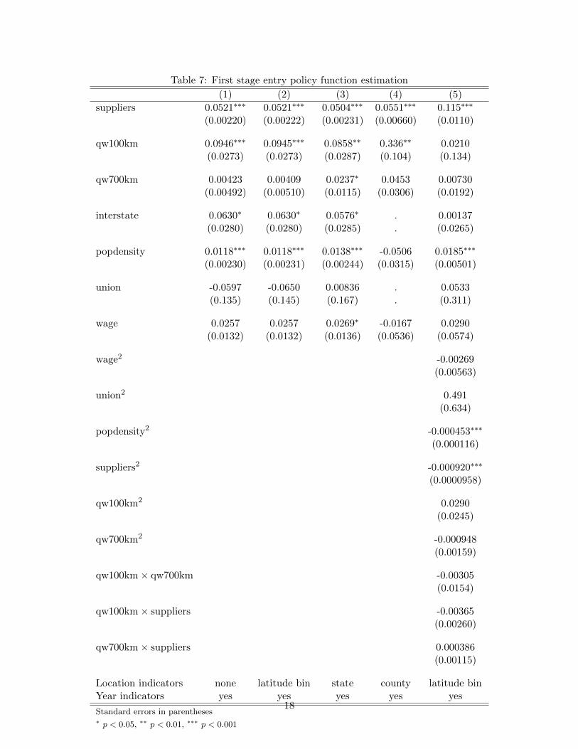
Table 7: First stage entry policy function estimation

(1) (2) (3) (4) (5)

suppliers 0.0521∗∗∗ 0.0521∗∗∗ 0.0504∗∗∗ 0.0551∗∗∗ 0.115∗∗∗

(0.00220) (0.00222) (0.00231) (0.00660) (0.0110)

qw100km 0.0946∗∗∗ 0.0945∗∗∗ 0.0858∗∗ 0.336∗∗ 0.0210(0.0273) (0.0273) (0.0287) (0.104) (0.134)

qw700km 0.00423 0.00409 0.0237∗ 0.0453 0.00730(0.00492) (0.00510) (0.0115) (0.0306) (0.0192)

interstate 0.0630∗ 0.0630∗ 0.0576∗ . 0.00137(0.0280) (0.0280) (0.0285) . (0.0265)

popdensity 0.0118∗∗∗ 0.0118∗∗∗ 0.0138∗∗∗ -0.0506 0.0185∗∗∗

(0.00230) (0.00231) (0.00244) (0.0315) (0.00501)

union -0.0597 -0.0650 0.00836 . 0.0533(0.135) (0.145) (0.167) . (0.311)

wage 0.0257 0.0257 0.0269∗ -0.0167 0.0290(0.0132) (0.0132) (0.0136) (0.0536) (0.0574)

wage2 -0.00269(0.00563)

union2 0.491(0.634)

popdensity2 -0.000453∗∗∗

(0.000116)

suppliers2 -0.000920∗∗∗

(0.0000958)

qw100km2 0.0290(0.0245)

qw700km2 -0.000948(0.00159)

qw100km× qw700km -0.00305(0.0154)

qw100km× suppliers -0.00365(0.00260)

qw700km× suppliers 0.000386(0.00115)

Location indicators none latitude bin state county latitude binYear indicators yes yes yes yes yes

Standard errors in parentheses∗ p < 0.05, ∗∗ p < 0.01, ∗∗∗ p < 0.001

18

Table 8: Transition of local characteristics

Southern Auto Alley Northern Auto AlleyLagged Mean Lagged Mean

variable coeff Constant Sq Error variable coeff Constant Sq Error

Population density 1.0336 0.0577 0.3669 0.9919 0.1489 0.5152

Wage 0.8925 0.5173 0.4692 0.8345 0.7897 0.5027

Assembly quantity with 100 km 0.8775 0.0322 0.1277 0.8646 0.0238 0.2584

Assembly quantity with 700 km 0.8649 0.5870 1.2381 0.6009 3.1980 1.3489

associated with receiving or sending intermediate goods. Nearby assembly plants increase

profitability, but only slightly.

For comparison, dynamic results are compared to estimates of the static model. Suppliers

in the dynamic model consider being in a region with high assembly quantity to be less

important. The static model explains the persistence of suppliers in Northern Auto Alley by

noting the high contemporaneous assembly production. In the dynamic model, suppliers see

the transition of assembly quantity within 700 kilometers and know that high current assembly

production is no guarantee of continued assembly production. Since suppliers persist in the

north even though they suspect assemblers will leave, the dynamic model must find other, less

transitory factors to explain the continued entry in the north. The dynamic model concludes

that agglomeration effects must be bigger and that union costs must be smaller than static

models would suggest.

Assembly quantity within 100 kilometers also is more important in the dynamic model

than in the static estimates. Areas with the highest concentration of assembly plants also have

the highest turnover rates and therefore the highest predicted exit rates and shortest expected

plant lifetime. Yet entrants still select these areas. The model concludes that entrants must

find the immediate proximity of assembly plants profitable enough to justify the higher hazard

rate caused by other variables.

Table 10 reports the marginal effect of a unit increase of each variable on the expected

number of new entrants in 2006 in a location with average state variables. The dynamic model

differs from the static model not just in coefficient values, but in that future state variable

19

Table 9: First stage exit policy function

(1) (2)

suppliers -0.00426 0.0504(0.00278) (0.0303)

qw100km 0.0918 -0.0772(0.0533) (0.408)

qw700km -0.0681∗∗∗ -0.292∗∗∗

(0.0150) (0.0730)

wage 0.0831∗ -0.114(0.0397) (0.214)

union 0.460 1.531(0.356) (0.934)

interstate -0.0371 -0.0350(0.0886) (0.0938)

popdensity 0.00480 0.0239∗

(0.00334) (0.0118)

suppliers2 -0.000101(0.000122)

qw100km2 0.0655(0.0517)

qw700km2 0.0183∗∗

(0.00565)

qw100km× qw700km -0.00328(0.0424)

qw100km× suppliers -0.00339(0.00341)

qw700km× suppliers -0.00432(0.00288)

wage2 0.0151(0.0203)

union2 -1.565(1.765)

popdensity2 -0.000441(0.000225)

northern auto alley 0.334∗∗∗ 0.319∗∗∗

(0.0852) (0.0896)

Year indicators yes yes

N 4973 4973

Standard errors in parentheses∗ p < 0.05, ∗∗ p < 0.01, ∗∗∗ p < 0.001

20

Table 10: Dynamic and myopic results

Static Dynamic(1) (2)

suppliers 0.0521∗∗∗ 0.192∗∗∗

(0.00222) (0.00802)

qw100km 0.0945∗∗∗ 0.318∗∗∗

(0.0273) (0.0831)

qw700km 0.00409 -0.0109(0.00510) (0.0144)

wage 0.0257 0.00431(0.0132) (0.0474)

union -0.0650 -0.0744(0.145) (0.397)

interstate 0.0630∗ 0.117(0.0280) (0.0709)

popdensity 0.0118∗∗∗ 0.0351∗∗∗

(0.00231) (0.00704)

Year indicators Yes YesLocation indicators latitude bin latitude bin

Standard errors in parentheses. Standard errors currently account

only for second stage and therefore are a lower bound.∗ p < 0.05, ∗∗ p < 0.01, ∗∗∗ p < 0.001

values are used to predict entry. The table calculates the effect of both a single period increase

in each variable while holding the rest of a supplier’s profit stream fixed and a permanent

proportional increase in the variable in all future periods. A one million vehicle increase in

nearby assembly production, the rough equivalent of three new assembly plants, brings up

the number of supplier plants entering each county by only a small fraction.

8 Counterfactuals

8.1 Simulation with counterfactual placement of assembly plants

The dynamic model can simulate supplier entry and exit starting from actual or counterfactual

conditions. The transition functions estimated in the first stage can be used to simulate

21

Table 11: Marginal effect on the number of new entrants

Static Dynamic model Dynamic modelmodel single period change permanent change

suppliers 0.022 0.054 0.093

qw100km 0.040 0.094 0.167

qw700km 0.002 -0.002 -0.005

wage 0.011 0.001 0.002

union -0.025 -0.019 -0.031

interstate 0.026 0.033 0.054

popdensity 0.005 0.010 0.016

Marginal effects at the average values, measured by

number of new entrants per period.

location characteristics in future periods, in much the same way that they were used in the

forward simulations in the estimation routine. Because the policy functions estimated in the

first stage are equilibrium objects, they too can be used in the forward simulation to simulate

the site selection of new entrants and the closure decisions of incumbents.

The model can be used for the exact counterfactual experiments policymakers should

consider. The additional number of suppliers brought to a jurisdiction by a successful bid

can be estimated by comparing model simulations where assembler proximity variables are

increased to reflect the new assembly plant locating in different sites.

The experiment here specifically moves the new Volkswagen assembly plant in Chat-

tanooga, Tennessee to Grand Rapids, Michigan. The counterfactual location was motivated

by press reports that before announcing their location decision, Volkswagen officials had con-

sidered three finalist sites in Alabama, Tennessee, and Michigan. Tennessee’s efforts to become

the host of the new plant included a subsidy bid reportedly costing $577 million.8 If a smaller

subsidy offer from Tennessee would have lead Volkswagen to place its plant in Michigan, this

counterfactual experiment answers how many suppliers Tennessee’s half billion dollar subsidy

8Pare, Mike. “VW Spends Most of $235 million in infrastructure aid.” Chattanooga Times Free Press.12 Oct 2011. The bid included $130 million in waived taxes that would not have existed without the plantanyway, but the rest of the subsidies represent real expenditures.

22

brought.

In the first model simulation all assembly plants are given their actual locations and

actual production quantities for 2011. (Since the new Volkswagen plant opened near the

end of 2011, I use an estimate of 150,000 units for its production count. This should form a

better basis for supplier expectations than the actual count from the last few months of 2011.)

From this, the assembly production within 100 kilometers and within 700 kilometers variables

are calculated. All other location characteristics start with their 2011 values. Following

Benkard, Bodoh-Creed, and Lazarev (2010), the first stage estimates of transitions and policy

function simulate the evolution in each county of the number of suppliers and of all location

characteristics, including assembly production nearby. The counterfactual simulation moves

the coordinates for the Volkswagen plant to those for Grand Rapids, Michigan. This results

in starting period values for assembly production within 100 kilometers and 700 kilometers

that are lower for counties near Chattanooga and higher for counties near Grand Rapids.

Otherwise, the procedure is identical to the model simulation. Both model and counterfactual

simulation were run 10,000 times; the difference in average supplier counts for each county

reflects the influence of the moved plant.

Table 12 reports the average supplier counts in the model and counterfactual simulations

summed for all counties in Tennessee. Both simulations predict a continued increase in the

Tennessee supplier base, though the growth is lower in the counterfactual that removes the

Volkswagen assembly plant. The two models diverge only slightly, never by more the 0.5 sup-

pliers (representing about 150 supplier jobs). The county with the largest difference between

model and counterfactual simulation, was Hamilton County, the home of the assembly plant.

Other nearby counties and counties throughout Tennessee with the largest existing supplier

bases were also among the places that benefited the most. A few counties in Tennessee even

had slightly more suppliers under the counterfactual, since the new assembly plant made

them relatively less attractive than counties nearer Chattanooga, which are close substitutes

to them. Nevertheless, almost all counties had fewer suppliers in the counterfactual in most

periods, though the effect everywhere was small.

The model on which these simulations are built assumes all parts suppliers value the

assembler proximity the same. In reality, different transportation costs for particular parts

23

Table 12: Supplier plant counts in the counterfactual simulation

Supplier countsPeriod Model Counterfactual

Tennessee0 (2011) 68.00 68.001 (2016) 74.64 74.272 (2021) 78.52 78.023 (2026) 80.57 80.14

likely cause some heterogeneity. A subset of parts suppliers with a much higher affinity for

nearby assembly plants would be more sensitive to the movement of assembly plants than

averages would suggest, so a next step is to test the robustness of these results with different

sub-classifications of the supplier parts industry.

8.2 Entry patterns without agglomeration

The second stage estimates emphasize the importance of a persistent supplier base to the

profits of other part suppliers. To see how these agglomeration benefits are driving entry,

suppose the profits of one new potential entrant do not depend on the number of suppliers in

its prospective locations. That is, let γn = 0 for this one entrant, preventing it from benefiting

from any spillovers or agglomeration benefits in excess of local competition or congestion

costs. Such an entrant will not affect the overall equilibrium being played or any suppliers

expectation of how the industry will evolve, so the first stage estimates will still represent the

equilibrium policy functions for all other suppliers. The one new entrant, however, will have

markedly different entry probabilities from the rest of its cohort.

Without net agglomeration benefits, a new potential entrant in 2006 would enter Michigan

with 6.9% probabilities, while the dynamic model predicts the average probability of entry in

Michigan at 28.2%. (Performing a similar experiment with a static model yields probabili-

ties of 5.9% and 15.9% respectively.) Agglomeration benefits are therefore important to the

maintenance of the persistent supplier base in Northern Auto Alley.

Probabilities and predictions under a counterfactual where no supplier can benefit from

spillovers cannot be calculated, because such an experiment would change enough entry

and exit policy functions. The Bajari, Benkard, and Levin (2007) methodology obtains its

24

tractability by not solving for equilibrium and by using the data to implicitly solve for the

equilibrium selection mechanism being used. Therefore, I am not able to calculate what the

new equilibrium policy functions would be and so cannot find the evolutionary paths of lo-

cation characteristics that suppliers expect. The experiment with one new entrant does hint

that the impact would be large and that entirely different equilibria would emerge in the

absence of peer agglomeration.

9 Conclusion

Durability and entry costs make selecting a site for plants a long term decision. An industry

migration increases the importance of dynamic concerns, which static models may miss. In

the case of motor vehicle parts suppliers, the static model underestimates the extent of peer

agglomeration benefits.

A model that can estimate the entry and closure decisions of parts suppliers can be used

to estimate the benefits of attracting assembly plants. It finds Tennessee’s expensive subsidies

of assembly plants have had little influence on the location decisions of parts suppliers.

25

References

Aguirregabiria, V., and P. Mira (2007): “Sequential Estimation of Dynamic DiscreteGames,” Econometrica, 75(1), 1–53.

Bajari, P., L. Benkard, and J. Levin (2007): “Estimating Dynamic Models of ImperfectCompetition,” Econometrica, 75(5), 1331–1370.

Benkard, L., A. Bodoh-Creed, and J. Lazarev (2010): “Simulating the Dynamic Effectsof Horizontal Mergers: U.S. Airlines,” Working paper, Yale University.

Brinkman, J., D. Coen-Pirani, and H. Sieg (2012): “Estimating a Dynamic EquilibriumModel of Firm Location Choices in an Urban Economy,” Working paper, Federal ReserveBank of Philadelphia.

Carlton, D. W. (1979): “Why New Firms Locate Where They Do: An Econometric Model,”in Interregional Movements and Regional Growth, ed. by W. C. Wheaton, pp. 13–50. UrbanInstitute, Washington.

Collard-Wexler, A. (2014): “Mergers and Sunk Costs: An Application to the Ready-MixConcrete Industry,” American Economic Journal: Microeconomics, 6(4), 407–47.

Dumais, G., G. Ellison, and E. L. Glaeser (2002): “Geographic Concentration as aDynamic Process,” Review of Economics and Statistics, 84(2), 193–204.

Ellison, G., and E. L. Glaeser (1997): “Geographic Concentration in U.S. ManufacturingIndustries: A Dartboard Approach,” Journal of Political Economy, 105(5), 889–927.

Ellison, G., E. L. Glaeser, and W. R. Kerr (2010): “What Causes Industry Agglom-eration? Evidence from Coagglomeration Patterns,” American Economic Review, 100(3),1195–1213.

Ericson, R., and A. Pakes (1995): “Markov-Perfect Industry Dynamics: A Framework forEmpirical Work,” Review of Economic Studies, 62(1), 53–82.

Greenstone, M., R. Hornbeck, and E. Moretti (2010): “Identifying AgglomerationSpillovers: Evidence from Winners and Losers of Large Plant Openings,” Journal of PoliticalEconomy, 118(3), 536–598.

Head, K., J. Ries, and D. Swenson (1995): “Agglomeration benefits and location choice:Evidence from Japanese maunfacturing investments in the United States,” Journal of Inter-national Economics, 38(3-4), 223–247.

Hirsch, B. T., and D. A. MacPherson (2003): “Union Membership and CoverageDatabase from the Current Population Survey: Note,” Industrial and Labor Relations Re-view, 56(2), 349–354.

Holmes, T. J. (1999): “How Industries Migrate When Agglomeration Economies Are Im-portant,” Journal of Urban Economics, 45(2), 240–263.

(2004): “Step-by-step migrations,” Review of Economic Dynamics, 7(1), 52–68.

26

Klier, T. H., and D. P. McMillen (2008): “Clustering of Auto Supplier Plants in theUnited States: Generalized Method of Moments Spatial Logit for Large Samples,” Journalof Business & Economic Statistics, 26(4), 460–471.

Neumark, D., B. Wall, and J. Zhang (2011): “Do Small Businesses Create More Jobs?New Evidence for the United States from the National Establishment Time Series,” Reviewof Economics and Statistics, 93(1), 16–29.

Pakes, A., M. Ostrovsky, and S. Berry (2007): “Simple Estimators for the Parametersof Discrete Dynamic Games (with Entry-Exit Examples),” RAND Journal of Economics,38(2), 373–399.

Rosenbaum, T. (2013): “Where Do Automotive Suppliers Locate and Why?,” Workingpaper, Yale University.

Rubenstein, J. M. (1992): The Changing US Auto Industry: a geographical analysis. Rout-ledge, London.

Ryan, S. P. (2012): “The Costs of Environmental Regulation in a Concentrated Industry,”Econometrica, 80(3), 1019–1061.

Seim, K. (2006): “An empirical model of firm entry with endogenous product-type choices,”The RAND Journal of Economics, 37(3), 619–640.

Smith, D., and R. Florida (1994): “Agglomeration and Industrial Location: An Economet-ric Analysis of Japanese-Affiliated Manufacturers in Automotive-related Industries,” Journalof Urban Economics, 36(1), 23–41.

Van Biesebroeck, J. (2003): “Productivity Dynamics with Technology Choice: An Appli-cation to Automobile Assembly,” Review of Economic Studies, 70(1), 167–198.

Woodward, D. (1992): “Locational Determinants of Japanese Manufacturing Start-ups inthe United States,” Southern Economic Journal, 58(3), 690–708.

27

A Data Appendix

A.1 Data Sources

Supplier plant locations come from the Dun’s Metalworking Directory for 1996 and before. For

2001 and latter, I use the Dun & Bradstreet Million Dollar Directory omitting plants with

fewer than 20 employees to match the Metalworking Directory’s inclusion criteria. Plants

are matched through time mostly by DUNS number, a permanent identifier of each plant.

Because the DUNS number sometimes changed without reason, plants that had no DUNS

number match in the subsequent year were also linked by address. (Cases in which matching

addresses lacked street numbers were linked only if the company name remained constant or a

corporate merger could be verified.) The Dun & Bradstreet data sometimes contains separate

records for divisions within the same plant, so exact address duplicates were merged together.

Wage data is from the Bureau of Labor Statistics’s Quarterly Census of Employment and

Wages (QCEW). The wages used are the county- and year-specific average weekly wage for

manufacturing plants (SIC 31-33). In counties where the manufacturing wage is unavailable,

the state average manufacturing wage is used.

Population estimates and county areas are from the US Census. Union membership rates

are state level from the Union Membership and Coverage Database. The construction of that

database from the Current Population Survey is described in Hirsch and MacPherson (2003).

Interstate highway indicators were constructed from map files published by the National

Atlas. Because of the stability in the interstate system since 1986, highway presence is a static

variable that uses current data. The location and production quantities for assembly plants

are from Ward’s Automotive Yearbook. (Pending the release of 2011 production figures, 2010

counts are used in their place.)

A.2 Quality of Plant Panel

Some early Dun & Bradstreet data are known to overreport employment, to overreport plant

counts, and to detect new entrants belatedly. Neumark, Wall, and Zhang (2011) find that in a

data set based on Dun & Bradstreet data from 1992 to 2006 employment measures are higher

than in the QCEW or the Current Employment Statistics (CES), but by county-industry are

28

Table 13: Supplier counts (alternate data source: CBP plants with 20+ employees)

1986 1991 1996 2001 2006 2009

Northern Auto Alley 418 486 535 602 619 496N Illinois 57 65 61 69 65 58N Indiana 45 67 80 99 97 64Michigan 208 241 262 275 284 235N Ohio 81 83 94 107 120 95Wisconsin 27 30 38 52 53 44

Southern Auto Alley 253 343 419 525 575 504Alabama 18 18 20 29 46 51Georgia 19 25 29 36 44 31S Illinois 11 17 15 18 22 20S Indiana 34 49 57 77 80 72Kentucky 15 34 47 69 77 73Mississippi 16 25 24 30 23 18North Carolina 36 41 59 66 66 59S Ohio 47 60 65 69 72 55South Carolina 9 18 33 50 54 52

Tennessee 48 56 70 81 91 73

highly correlated to both the QCEW and CES.

Table 3 shows the state-by-state count of plants with at least twenty employees and a

primary SIC code of 3714 from the Dun & Bradstreet. Table 14 gives the same information,

except using data from the County Business Patterns. The two data sets were produced with

different methodologies and in different months, but their counts are broadly similar. In a

few states and years counts differ by more than a third, but the pattern of plateauing plant

counts in northern auto alley and dramatically increasing counts in southern auto alley is seen

in both data sets.

29

Figure 1: Supplier employment in auto alley and assembly plants in 1986. Squares indicateassembly plant locations. Each dot represents employment of 200 at supplier plants.

30

Figure 2: Supplier employment in auto alley and assembly plants in 2011. Squares indicateassembly plant locations. Each dot represents employment of 200 at supplier plants.

31