mide: a macroeconomic multisectoral model of...
TRANSCRIPT

MIDE: A MACROECONOMIC MULTISECTORAL MODEL
OF THE SPANISH ECONOMY
by
Jeffrey Francis Werling
Dissertation submitted to the Faculty of the Graduate Schoolof The University of Maryland in partial fulfillment
of the requirements for the degree ofDoctor of Philosophy
1992
Advisory Committee:
Professor Clopper Almon, Chairman/AdvisorProfessor Roger BetancourtProfessor Christopher ClagueProfessor Paul WeinsteinProfessor Lee Preston

MIDE: A MACROECONOMIC MULTISECTORAL MODEL
OF THE SPANISH ECONOMY
Abstract
When Spain joined the European Community in 1986, its economy began to bustle.
For the years 1986 through 1991, its GDP growth was substantially higher than any of its
EC partners. A dramatic acceleration in investment paced this growth. However, while
imports have exploded, export growth has been disappointing, and a large current account
deficit has evolved. Furthermore, inflation is above the EC average, but unemployment,
originally produced by stagnation in the early eighties, remains disturbingly high. These
circumstances have produced uncertainty over the future course of the economy, especially
their implications in the context of the continuing EC integration process.
Comprehensive empirical models can increase the understanding of the evolution of an
economy, and decrease uncertainty surrounding the future, by providing a bridge between
economic theory and the real world. This work describes the construction and application
of a macroeconomic, dynamic, multisectoral simulation and forecasting model of the Spanish
economy (MIDE). Using the data and accounting structure of the Spanish 43 sector input-
output table for 1980 and the annual national accounts, MIDE is constructed by combining
the classical input-output formulation with extensive use of regression analysis. The model
is a comprehensive representation of economy, so it can analyze the economy wide effects
of macroeconomic developments. However, the framework allows for a highly
disaggregated treatment of economic variables. For example, total capital investment, total
imports and total income are not determined directly but are computed from the sum of their
parts: investment in specific goods, imports by production branch, and labor compensation

by industry. This "bottom-up" approach gives the model the ability to describe the effects
of developments in one industry on related sectors and the overall economy.
Following a general outline of MIDE’s structure, the dissertation presents functional
specifications and estimation results for the model’s macroeconomic and commodity level
econometric behavioral equations. MIDE is part of the INFORUM system of trade-linked
multisectoral models. Using this system, the study illustrates the impacts on the Spanish
economy of the European single market which is to begin in 1993. Once the various single
market measures are integrated into the model, a forecast to the year 2000 is presented. The
results demonstrate that the Spanish economy can reach "monetary convergence" with the
rest of the EC without suffering significant decreases in growth of income and employment.
Detailed industry-level projections indicate the potential course of structural change. They
illustrate a maturing economy becoming even more integrated with the international
economy.

PREFACE
Three years ago, I was given the opportunity to move to Madrid and write my
dissertation concerning the construction of the INFORUM model of the Spanish economy
(MIDE). This model serves as the focus of economic research and consulting activities at
the Center for Economic Studies of the Fundación Tomillo. The development of the model
was particularly challenging, since when I arrived in Madrid I knew very little about Spain
or its economy. The work also provided me with a unique learning experience, since the
Spanish economy is presently one of the most dynamic and fastest growing in the
industrialized world. However, this dissertation is only one product of the marvelous
experience of being a guest of the Spanish people. The most important souvenir that my
family and I will take from Spain is the memory of the hospitality and kindness extended
to us throughout our stay.
All completing doctoral students owe debts to many people. I am certain, however, that
my case is distinguished by the large number of people who assisted me in this endeavor.
The Spanish Ministry of Education and Science provided considerable support for my
research over two years. I would also like to thank my colleagues at INFORUM, Margaret
McCarthy, who taught me many tricks of the trade, and Doug Nyhus and Costas Christou
who formulated the Europe 1992 scenarios which formed the foundation for Chapter 8 of
this work. At Fundación Tomillo, I enjoyed invaluable guidance and assistance from
Vincente Antón, Juan Carlos Collado, Antonio Diaz, Jose Fierros and Mario Tomba. There
is no doubt that the work could not have been completed without them. I am also indebted
to Carlos Nuñez and Elena Alonso for cheerfully performing tedious research assistance, and
Jose Muñoz, who helped me deal with the day-to-day business of life in a foreign country.

I would also like to thank Maurizio Grassini, who, in two short trips to Madrid, taught me
more about interindustry modeling than I would have learned in several months on my own.
I am much indebted to Clopper Almon for recommending me for the position at
Fundación Tomillo, and for allowing me the independence to conduct my dissertation
research several thousand miles away. I hope that I have justified his confidence in my
abilities. The greatest thanks of all must be reserved for Javier Lantero, whose patience,
generosity and foresight provided me the opportunity not only to write this dissertation, but
also to enjoy three wonderul years with the Spanish people. While I know that I could
never repay his kindness in full, I hope that my work at Fundación Tomillo will establish
a solid base for a fruitful and enduring economic research program.
Madrid, May 14, 1992

TABLE OF CONTENTS
Section Page
PREFACE . . . . . . . . . . . . . . . . . . . . . . . . . . . . . . . . . . . . . . . . . . . . . . . . . . . . . . i
LIST OF TABLES . . . . . . . . . . . . . . . . . . . . . . . . . . . . . . . . . . . . . . . . . . . . . . v
LIST OF FIGURES . . . . . . . . . . . . . . . . . . . . . . . . . . . . . . . . . . . . . . . . . . . . . . vii
CHAPTER 1: INTRODUCTION . . . . . . . . . . . . . . . . . . . . . . . . . . . . . . . . . . . . . 1
CHAPTER 2: HISTORICAL OVERVIEW AND SECTORAL CHARACTERISTICSOF THE SPANISH ECONOMY . . . . . . . . . . . . . . . . . . . . . . . . . . . . . . . . . . 82.1 Overview of the Spanish Economy, 1960-1991 . . . . . . . . . . . . . . . . . . . . . 8
The Years of Prosperity: 1960-1974 . . . . . . . . . . . . . . . . . . . . . . . . . . . . 11Economic Crisis: 1975-1985 . . . . . . . . . . . . . . . . . . . . . . . . . . . . . . . . . 16EC Integration and Economic Boom: 1986-1990 . . . . . . . . . . . . . . . . . . . 20Prospects for the Modern Spanish Economy . . . . . . . . . . . . . . . . . . . . . . 23
2.2 A Sectoral Description of the Spanish Economy . . . . . . . . . . . . . . . . . . . . 33Sector 1: Agriculture, Forestry and Fishing . . . . . . . . . . . . . . . . . . . . . . . 33Sectors 2-5: Energy . . . . . . . . . . . . . . . . . . . . . . . . . . . . . . . . . . . . . . . 37Sectors 6-25: Manufacturing . . . . . . . . . . . . . . . . . . . . . . . . . . . . . . . . . 39Sector 26: Construction . . . . . . . . . . . . . . . . . . . . . . . . . . . . . . . . . . . . . 52Sectors 27-39: Private Sector Services . . . . . . . . . . . . . . . . . . . . . . . . . . 53Sectors 40-42: Public Sector Services . . . . . . . . . . . . . . . . . . . . . . . . . . . 58Tourism . . . . . . . . . . . . . . . . . . . . . . . . . . . . . . . . . . . . . . . . . . . . . . . . 60
CHAPTER 3: EMPIRICAL ECONOMIC MODELS OF THE SPANISHECONOMY . . . . . . . . . . . . . . . . . . . . . . . . . . . . . . . . . . . . . . . . . . . . . . . . 633.1 Macroeconometric Models . . . . . . . . . . . . . . . . . . . . . . . . . . . . . . . . . . . 643.2 Classic Input-Output Models . . . . . . . . . . . . . . . . . . . . . . . . . . . . . . . . . . 683.3 Computable General Equilibrium Models . . . . . . . . . . . . . . . . . . . . . . . . . 713.4 Macroeconomic Multisectoral Models . . . . . . . . . . . . . . . . . . . . . . . . . . . 72
CHAPTER 4: GENERAL EQUILIBRIUM FRAMEWORK OF THE MIDEMODEL . . . . . . . . . . . . . . . . . . . . . . . . . . . . . . . . . . . . . . . . . . . . . . . . . . . 764.1 The Production Block . . . . . . . . . . . . . . . . . . . . . . . . . . . . . . . . . . . . . . 824.2 The Price-Income Block . . . . . . . . . . . . . . . . . . . . . . . . . . . . . . . . . . . . 914.3 The Accountant . . . . . . . . . . . . . . . . . . . . . . . . . . . . . . . . . . . . . . . . . 1014.4 Criteria for Equation Specification and Evaluation of Econometric Results 107
CHAPTER 5: EQUATION SPECIFICATION AND ESTIMATION: CONSUMPTIONAND FIXED INVESTMENT . . . . . . . . . . . . . . . . . . . . . . . . . . . . . . . . . . . 116

TABLE OF CONTENTS (continued)
Section Page
5.1 Private Consumption . . . . . . . . . . . . . . . . . . . . . . . . . . . . . . . . . . . . . . 116Aggregate Private National Consumption . . . . . . . . . . . . . . . . . . . . . . . 117An Equation System for Consumption by Commodity Categories . . . . . . 124Estimation of the System for Spain . . . . . . . . . . . . . . . . . . . . . . . . . . . . 132
5.2 Fixed Capital Investment . . . . . . . . . . . . . . . . . . . . . . . . . . . . . . . . . . . 144Non-residential Investment . . . . . . . . . . . . . . . . . . . . . . . . . . . . . . . . . . 144Residential Construction . . . . . . . . . . . . . . . . . . . . . . . . . . . . . . . . . . . 167
CHAPTER 6: ECONOMETRIC SPECIFICATION AND ESTIMATES: FOREIGNTRADE, PRODUCTIVITY AND EMPLOYMENT . . . . . . . . . . . . . . . . . . . 1706.1 International trade . . . . . . . . . . . . . . . . . . . . . . . . . . . . . . . . . . . . . . . . 170
A Sectoral Analysis of Spanish Foreign Trade . . . . . . . . . . . . . . . . . . . . 174Imports . . . . . . . . . . . . . . . . . . . . . . . . . . . . . . . . . . . . . . . . . . . . . . . 181Exports . . . . . . . . . . . . . . . . . . . . . . . . . . . . . . . . . . . . . . . . . . . . . . . 195Tourism . . . . . . . . . . . . . . . . . . . . . . . . . . . . . . . . . . . . . . . . . . . . . . . 201
6.2 Productivity and Employment . . . . . . . . . . . . . . . . . . . . . . . . . . . . . . . . 204Labor Productivity . . . . . . . . . . . . . . . . . . . . . . . . . . . . . . . . . . . . . . . 208Annual Hours Worked per Employee . . . . . . . . . . . . . . . . . . . . . . . . . . 215
CHAPTER 7: EQUATION SPECIFICATION AND ESTIMATION:EMPLOYMENT AND CAPITAL INCOME . . . . . . . . . . . . . . . . . . . . . . . . 2207.1 Employment Income . . . . . . . . . . . . . . . . . . . . . . . . . . . . . . . . . . . . . . 222
The Aggregate Wage Equation . . . . . . . . . . . . . . . . . . . . . . . . . . . . . . . 225Sectoral Wage Equations . . . . . . . . . . . . . . . . . . . . . . . . . . . . . . . . . . . 233
7.2 Capital Income . . . . . . . . . . . . . . . . . . . . . . . . . . . . . . . . . . . . . . . . . . 234
CHAPTER 8: A FORECAST FOR THE SPANISH ECONOMY TO THE YEAR2000: THE IMPACT OF EUROPEAN COMMUNITY INTEGRATION . . . . . 2528.1 Exogenous Assumptions for the Forecast to 2000 . . . . . . . . . . . . . . . . . . 2538.2 The Impact of the European Single Market on the Spanish Economy . . . . 256
The Elimination of Customs Controls . . . . . . . . . . . . . . . . . . . . . . . . . . 264Opening of Public Procurement to Foreign Suppliers . . . . . . . . . . . . . . . 268Deregulation of Financial Services . . . . . . . . . . . . . . . . . . . . . . . . . . . . 275Supply Effects . . . . . . . . . . . . . . . . . . . . . . . . . . . . . . . . . . . . . . . . . . 277Fiscal Harmonization . . . . . . . . . . . . . . . . . . . . . . . . . . . . . . . . . . . . . 280Spain in the Single Market - The Total Impact . . . . . . . . . . . . . . . . . . . 282
8.3 A MIDE Forecast to the Year 2000 . . . . . . . . . . . . . . . . . . . . . . . . . . . . 293
CHAPTER 9: CONCLUSIONS AND DIRECTIONS FOR FURTHER WORK . . . 313
APPENDIX: THE DATA BASE OF THE MIDE MODEL . . . . . . . . . . . . . . . . . 317
REFERENCES . . . . . . . . . . . . . . . . . . . . . . . . . . . . . . . . . . . . . . . . . . . . . . . . 338

LIST OF TABLES
Table Page
2.1: Real Gross Domestic Product and Components,Other Economic Indicators, 1960-1991 . . . . . . . . . . . . . . . . . . . . . . . 10
2.2: Sectoral Proportion of GDP and Employment, 1960-1989. . . . . . . . . . . . . 122.3: Total and Direct Net Foreign Investment into Spain, 1982-90 . . . . . . . . . . 222.4: Program of Trade Liberalization Under Spain’s EC Membership, 1986-93 . 242.5: European Community Indicators of Monetary Convergence,
Year End 1991 . . . . . . . . . . . . . . . . . . . . . . . . . . . . . . . . . . . . . . . 282.6: Percentage Shares of Value Added and Employment for the Production
Sectors of the MIDE Model, 1980 and 1987 . . . . . . . . . . . . . . . . . . . 342.7: Foreign Trade Indicators for Production Sectors of the MIDE Model, 1987 . 352.8: Inflation Rate for Consumption Price Indices for
Type of Products, 1985-90 . . . . . . . . . . . . . . . . . . . . . . . . . . . . . . . 554.1: Components and Influences of the Production Block . . . . . . . . . . . . . . . . 904.2: Components and Influences of Price-Income Block . . . . . . . . . . . . . . . . . 994.3: GDP Identities of the MIDE Model . . . . . . . . . . . . . . . . . . . . . . . . . . . 1004.4: Macroeconomic Identities of the Accountant . . . . . . . . . . . . . . . . . . . . . 1024.5: Influences on Endogenous Macroeconomic Variables of the Accountant. . 1045.1: Estimation Results for Private National Consumption . . . . . . . . . . . . . . . 1225.2: Income-Compensated Price Elasticity Formulae for the
Almon Consumption System . . . . . . . . . . . . . . . . . . . . . . . . . . . . . 1315.3: Summary of Commodity Consumption Equations . . . . . . . . . . . . . . . . . . 1355.4: Consumption Elasticity Comparisons between HERMES-España
and the MIDE Model . . . . . . . . . . . . . . . . . . . . . . . . . . . . . . . . . . 1415.5: Consumption Elasticity Comparisons between Abadía (1984)
and the MIDE Model . . . . . . . . . . . . . . . . . . . . . . . . . . . . . . . . . . 1435.6: Fixed Capital Non-Residential Investment, 1970-89 . . . . . . . . . . . . . . . . 1456.1: Summary of Import Regression Results . . . . . . . . . . . . . . . . . . . . . . . . . 1826.2: Import Elasticity Comparisons between Fernandez-Sebastián
and the MIDE Model . . . . . . . . . . . . . . . . . . . . . . . . . . . . . . . . . . 1936.3: Summary of Merchandise Export Regression Results . . . . . . . . . . . . . . . 1976.4: Summary of Service Export Regression Results . . . . . . . . . . . . . . . . . . . 2006.5: Export Elasticity Comparisons between Fernandez-Sebastián
and the MIDE Model . . . . . . . . . . . . . . . . . . . . . . . . . . . . . . . . . . 2016.6: Summary of Labor Productivity Equation Results . . . . . . . . . . . . . . . . . . 2146.7: Summary of Hours per Worker-year Equations . . . . . . . . . . . . . . . . . . . 2187.1: Summary of Sectoral Wage Equations . . . . . . . . . . . . . . . . . . . . . . . . . 2357.2: Estimation results for sectoral gross profit equations:
Manufacturing and private services . . . . . . . . . . . . . . . . . . . . . . . . . . . . 2427.3: Estimation results for sectoral gross profit equations:
Commercial and residential rents and Public services . . . . . . . . . . . . 2518.1: Assumptions for Exogenous Variables of the MIDE Model, 1990-2000 . . 2548.2: Potential Economic Gains for EC from Completing the Internal Market . . 259

LIST OF TABLES (continued)
Table Page
8.3: Share of the Cost of the Administrative Formalities Borneby Firms in the Value of Bilateral Trade Flows . . . . . . . . . . . . . . . 265
8.4: Elimination of Border Controls - Comparison toSpain With Borders Case . . . . . . . . . . . . . . . . . . . . . . . . . . . . . . . 267
8.5: Shocks Introduced into the HERMES Model forOpening up of Public Procurement . . . . . . . . . . . . . . . . . . . . . . . . . 270
8.6: MIDE Model Sectors Effected by the Direct Impactsof the Open Public Procurement Simulation . . . . . . . . . . . . . . . . . . 271
8.7: Opening of Public Procurement - Comparison toSpain With Borders Case . . . . . . . . . . . . . . . . . . . . . . . . . . . . . . . 274
8.8: Financial Liberalization - Comparison to Spain With Borders Case . . . . . 2768.9: Decrease in Costs of Production as a Result of Increased
Competition and the Exploitation of Economies of Scale . . . . . . . . . 2788.10: Supply Effects - Comparison to Spain With Borders Case . . . . . . . . . . . . 2798.11: Fiscal Harmonization - Comparison to Spain With Borders Case . . . . . . . 2828.12: Spain in the European Single Market: The Total Impact
of Europe 1992 - Comparison to Spain With Borders Case . . . . . . . . 2838.13: Europe 1992: Comparison Among MIDE and Other Studies . . . . . . . . . . 2848.14: Sectoral Real Outputs and the European Single Market -
Comparison to Spain With Borders Case . . . . . . . . . . . . . . . . . . . . 2868.15: Sectoral Production Prices and the European Single Market -
Comparison to Spain With Borders Case. . . . . . . . . . . . . . . . . . . . . 2878.16: Sectoral Employment and the European Single Market -
Comparison to Spain With Borders Case . . . . . . . . . . . . . . . . . . . . 2888.17: Real Sectoral Exports and the European Single Market -
Comparison to Spain With Borders Case . . . . . . . . . . . . . . . . . . . . 2898.18: Real Sectoral Imports and the European Single Market -
Comparison to Spain With Borders Case . . . . . . . . . . . . . . . . . . . . 2908.19: Spain in the Single Market, MIDE Forecast to 2000 . . . . . . . . . . . . . . . . 2948.20: MIDE Model Projections - Constant Price Output by Production Sector. . . 3038.21: MIDE Model Projections - Output Prices by Production Sector . . . . . . . . 3048.22: MIDE Model Projections - Employment by Production Sector . . . . . . . . . 3058.23: MIDE Model Projections - Exports by Production Sector . . . . . . . . . . . . 3068.24: MIDE Model Projections - Imports by Production Sector . . . . . . . . . . . . 3078.25: MIDE Model Projections - Labor Compensation by Production Sector . . . 3088.26: MIDE Model Projections - Gross Profits by Production Sector . . . . . . . . 3098.27: MIDE Model Projections - Real Private Interior Consumption by
Commodities . . . . . . . . . . . . . . . . . . . . . . . . . . . . . . . . . . . . . . . . 3108.28: MIDE Model Projections - Consumption Prices by Commodity . . . . . . . . 3118.29: MIDE Model Projections - Fixed Capital Investment . . . . . . . . . . . . . . . 3128.30: MIDE Model Projections - Prices of Fixed Capital Investment . . . . . . . . 312

LIST OF FIGURES
Figure Page
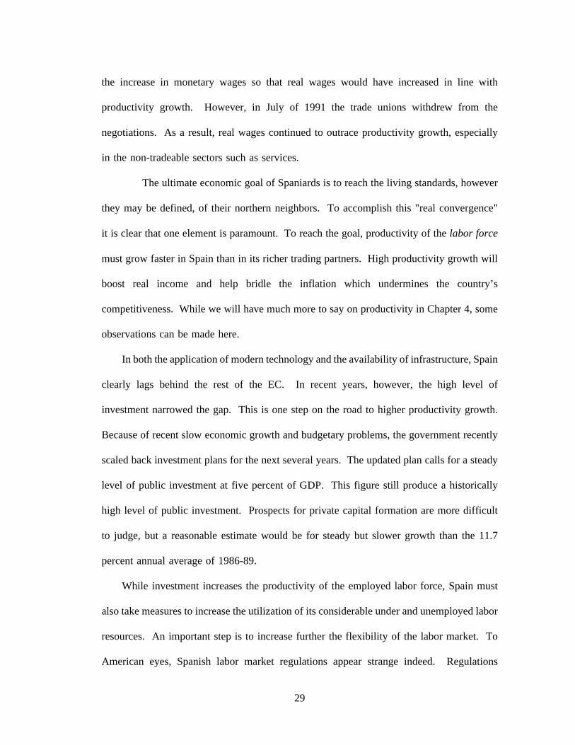
2.1: Real Gross Domestic Product, 1960-91 . . . . . . . . . . . . . . . . . . . . . . . . . . 92.2: Current Account Balance as a Percentage of GDP, 1960-91 . . . . . . . . . . . 92.3: Real Wages and Labor Productivity, 1965-90 . . . . . . . . . . . . . . . . . . . . . 182.4: Shares of Wages and Profits in Value Added at Factor Cost, 1965-90 . . . . 182.5: Employment and the Labor Force, 1964-91 . . . . . . . . . . . . . . . . . . . . . . . 202.6: Sector 6 Metal mining and metals processing, 1970-89 . . . . . . . . . . . . . . 432.7: Sector 7 Nonmetallic minerals and products, 1970-89. . . . . . . . . . . . . . . . 432.8: Sector 8 Chemicals, 1970-89. . . . . . . . . . . . . . . . . . . . . . . . . . . . . . . . . . 442.9: Sector 9 Metal products, 1970-89 . . . . . . . . . . . . . . . . . . . . . . . . . . . . . . 442.10: Sector 10 Industrial and agricultural machinery, 1970-89 . . . . . . . . . . . . . 452.11: Sector 11 Office machines, computers and instruments, 1970-89 . . . . . . . . 452.12: Sector 12 Electric and electronic equipment and material, 1970-89 . . . . . . 462.13: Sector 13 Motor vehicles and engines, 1970-89 . . . . . . . . . . . . . . . . . . . 472.14: Sector 14 Other transportation equipment, 1970-89 . . . . . . . . . . . . . . . . . . 472.15: Sectors 15-19 Food, beverages and tobacco products, 1970-89 . . . . . . . . . . 482.16: Sector 20-21 Textiles, clothing, leather products and footwear, 1970-89 . . . 502.17: Sector 22 Wood, wood products and furniture, 1970-89 . . . . . . . . . . . . . . 502.18: Sector 23 Paper, paper products and publishing, 1970-89 . . . . . . . . . . . . . 512.19: Sector 24-25 Plastic and rubber products, Other
manufactured products, 1970-89. . . . . . . . . . . . . . . . . . . . . . . . . . . . 512.20: Sector 26 Construction, 1970-90. Proportions of value added
in GDP and employment in total employment . . . . . . . . . . . . . . . . . . 522.21: Combined government deficit as percentage of the GDP, 1965-90 . . . . . . . 592.22: Gross Tourism Receipts and Payments, 1960-90 . . . . . . . . . . . . . . . . . . . 614.1: Input-Output Accounting Framework for the MIDE Model . . . . . . . . . . . . 774.2: Solution process of the MIDE Model . . . . . . . . . . . . . . . . . . . . . . . . . . . 815.1: Real Private National Consumption Equation, 1967-90. . . . . . . . . . . . . . . 1235.2: Regression Fits for Commodity Consumption Equations . . . . . . . . . . . . . 1395.3: Summary Regression Results for Investment in Industrial machinery . . . . 1545.4: Summary Regression Results for Investment in Metal products . . . . . . . . 1595.5: Summary Regression Results for Investment in Agricultural machinery . . 1605.6: Summary Regression Results for Investment in Office machines,
computers and precision instruments . . . . . . . . . . . . . . . . . . . . . . . 1615.7: Summary Regression Results for Investment in Electric and
electronic equipment . . . . . . . . . . . . . . . . . . . . . . . . . . . . . . . . . . . 1625.8: Summary Regression Results for Investment in Motor vehicles . . . . . . . . 1635.9: Summary Regression Results for Investment in
Other transport machinery . . . . . . . . . . . . . . . . . . . . . . . . . . . . . . . 1645.10: Summary Regression Results for Investment in
Non-residential construction . . . . . . . . . . . . . . . . . . . . . . . . . . . . . 1655.11: Summary Regression Results for Investment in Other products . . . . . . . . 1665.12: Summary Regression Results for Residential construction . . . . . . . . . . . . 169

LIST OF FIGURES (continued)
Figure Page
6.1: Import Equation Selection Process . . . . . . . . . . . . . . . . . . . . . . . . . . . . 1886.2: Regression Fits for Import Equations . . . . . . . . . . . . . . . . . . . . . . . . . . 1916.3: Estimation Results for Imports and Exports of Tourism, 1971-90 . . . . . . . 2036.4: Productivity growth: GDP/employment vs.
GDP/labor force, 1965-90 . . . . . . . . . . . . . . . . . . . . . . . . . . . . . . . 2066.5: Regression Fits for Hours per Worker-year Equations . . . . . . . . . . . . . . . 2197.1: Average Nominal Wage Growth, 1965-1991 . . . . . . . . . . . . . . . . . . . . . 2247.2: The Unemployment Rate and Its Lagged Four Year
Moving Average, 1970-91 . . . . . . . . . . . . . . . . . . . . . . . . . . . . . . . 2287.3: Estimation Results for Aggregate Wage Equation . . . . . . . . . . . . . . . . . . 2328.1: Sectoral Impacts of European Single Market . . . . . . . . . . . . . . . . . . . . . 2918.2: Value Added and Employment Shares by Major Sectors,
1986, 1990, 1994, 1998 . . . . . . . . . . . . . . . . . . . . . . . . . . . . . . . . 2998.3: Imports Percentage of Domestic Demand, Export
Percentage of Output, 1986, 1990, 1994, 1998 . . . . . . . . . . . . . . . . . 300

CHAPTER 1: INTRODUCTION
Empirical models offer a fruitful approach to understand an economy. In the first place,
their construction forces the analyst to examine each and every part of the economic process.
Further, it tests whether his understanding of the parts adds up to an understanding of the
whole. Once a model is built, the presentation of its structure and empirical results motivate
and focus economic discussions by economists and non-economists alike. In my experience,
economic forecasts never fail to attract interesting analysis and opinions from any group of
informed observers. Careful and honest use of models has even been known to be useful
to economists, business managers or government officials for quantitative analysis and
decision making.
This work presents the construction and application of a macroeconomic, dynamic,
multisectoral forecasting model of the Spanish economy (MIDE).1 The foundation of the
MIDE model is a 43 sector input-output table embedded in the structure of the Spanish
national accounts. Combining the classical input-output formulation with extensive use of
regression analysis, MIDE employs a "bottom-up" approach to macroeconomic modeling.
For example, total capital investment, total imports and total wage income are not projected
directly but are computed from the sum of their parts: investment by specific goods, imports
by production branch, and labor compensation by industry. This bottom-up technique
possesses several desirable properties for analyzing an economy. First, the model works like
the actual economy, building the macroeconomic totals from details of industry activity,
rather than distributing predetermined macroeconomic quantities among industries. Second,
1 In Spanish, MIDE stands for El Modelo Macroeconómico Intersectorial de España.It is also the third person present tense of the verb medir, "to measure."
1

the model describes the effects of changes in one industry, such as increasing productivity
or changing input-output coefficients, on other, related sectors and the aggregate quantities.
Third, parameters in the behavioral equations differ among products, reflecting differences
in consumer preferences, price elasticities in foreign trade, and industrial structure. Fourth,
the detailed level of disaggregation permits the modeling of prices by industry, allowing one
to explore the causes of relative price changes.
Another important feature of the MIDE model is the importance given to the dynamic
determination of endogenous variables. For example, investment depends on a distributed
lag in the output growth of investing industries. Therefore, MIDE model solutions are not
static, but are fully capable of projecting a time path for the endogenous quantities. Finally,
the MIDE model is linked to other, similar models with the INFORUM2 international trade
model. Countries included in this system include the U.S., Japan, and major European
economies. Through this system, sectoral exports and imports of the Spanish economy
respond to sectoral level demand and price variables projected by models of its trading
partners. In brief, the MIDE model is particularly suited for examining and assessing the
macroeconomic impacts of the changing composition of consumption, production, foreign
trade and employment as the economy grows through time.
MIDE consists of three components: the production block, the price-income block, and
the macroeconomic accountant. The production block estimates final demand using
individual, econometrically estimated behavioral equations for each of the commodity and
2 INFORUM is the Interindustry Forecasting Project at the University of Maryland,U.S.A., founded by Clopper Almon in 1967. This research group has, in collaboration withother international partners, developed a foreign trade linked system of models for thecountries of the Austria, Belgium, Canada, France, Italy, Japan, Mexico, South Korea, Spain,the United States and West Germany. Several other country models, including ones forPoland and the United Kingdom, have been developed and await integration into theinternational model.
2

sectoral-specific quantities. Real output by industry is then determined with the Leontief
input-output identity, where the interindustry technical coefficients vary over time. The
price-income block computes industry income and prices using behavioral equations for
primary input costs and an input-output price identity. The accountant determines the
magnitude of national income and distributes this income among households, governments
and firms. It also computes the current account and government balances. Relationships
specified among the variables of the three model components close the model.
The addition of the MIDE model to the small inventory of empirical models of Spain
is particularly timely. The MIDE model is the only multisectoral, dynamic, macroeconomic
model of the Spanish economy with significant (i.e., over twelve sectors) disaggregation.
Therefore, it can be used for applications where other, existing models are inadequate.
Specifically, I employ the MIDE model here to investigate the short and longer-run
macroeconomic and industry level implications of Spanish integration in the European
Community (EC) single market.
Along with the rest of Europe, the Spanish economy is in the midst of transition. In
1975, Spain entered a long period of stagnation which produced a restructuring of its
production base and high unemployment. Since joining the EC in 1986, however, the
economy has been growing rapidly. An acceleration in investment for capital goods, non-
residential construction and housing paced this growth. However, foreign trade has become
a concern. Strong interior demand, coupled with EC mandated trade liberalization, led to
dramatic import increases which have not been compensated with similar export growth.
As a result, the current account registers a fat deficit. Recent increases in real wages and
steady appreciation of the peseta has exacerbated the problem. This deficit produces
uneasiness surrounding the future of the economy.
3

The most important influence on the course of the Spanish economy for the next decade
will be the continuing integration of the EC. The Europe 1992 program will eliminate all
barriers to trade, capital and labor movements between the Community countries. Many
Spaniards feel that with the arrival of the single market in 1993, the external imbalance will
become unsustainable and another deep retraction will be required. This prospect is most
discouraging because, despite five years of vigorous growth, the official unemployment rate
still stands at over 15 percent.
Another preoccupation among the Spaniards concerns whether the nation will reach
"monetary convergence" with the rest of the EC in preparation for Economic and Monetary
union (EMU). Under agreements made in the recent EC Maastricht summit, the union will
start in 1997 if a majority of the current EC members meet the "convergence criteria"
required to join. Currently, the magnitudes of Spain’s inflation and interest rates, as well
as its government budget deficit, would exclude it from the union. While the nation has five
years to progress on these fronts, it is by no means certain that convergence can be
accomplished.
The MIDE model, as a comprehensive representation of the Spanish economy, is a
convenient tool for investigation of the impact of EC integration. Of course, the effects of
the EC single market will differ across sectors of the economy. For example, since EC
membership in 1986, high-growth, export-orientated industries, such as automobiles, have
benefitted. On the other hand, import-competing industries, such as textiles and apparel,
have suffered significant market penetration into their previously closed markets. Existing
aggregate models of the Spanish economy cannot project the course of individual industries,
nor can they consider the macroeconomic impacts of sectoral developments. As stressed
above, the multisectoral framework of the MIDE model provides both of these capabilities.
4
Moreover, the dynamic character of the model permits a quantification of the short-run costs
which may accompany the long-run benefits of Spain’s full integration into the European
single market. This is in contrast to disaggregated models which contribute a comparative
static approach to the issue. Finally, the inclusion of the MIDE model in the INFORUM
trade-linkage system provides a particularly useful framework for assessing the effects of
continuing European integration, since developments in the economies of Spain’s trading
partners can be taken into account.
I would like to emphasize that, although MIDE is the Spanish representative of the
INFORUM system, its construction was not simply an application of a general model form.
The specification and estimation of the MIDE model explicitly integrates particular
characteristics of the Spanish economy. This strategy is indispensable in order to assure the
relevance and realism of the model. Moreover, because of the dearth of disaggregated
econometric studies of the Spanish economy, some of the sectoral-level equation estimations
constitute unique studies on their own. I hope that this work will be found useful to
researchers of both the Spanish and of other economies.
The specification and estimation of any empirical model is necessarily dependent on the
historic evolution and institutional framework of the economy examined. The second
chapter of this dissertation, therefore, provides a brief history and a current assessment of
the modern Spanish economy. Touching upon macroeconomic, institutional and sectoral
characteristics, this chapter supplies the raw material for construction of the MIDE model
and a point of reference for its projections. The description of the MIDE model found here
will refer to other models of the Spanish economy. To provide a background for these
references, the third chapter presents a survey of the other empirical models of the Spanish
economy, comparing and contrasting these models with the MIDE model.
5

The fourth chapter opens with a presentation of the general-equilibrium framework and
solution process of the MIDE model. It discusses each of the model’s three components
separately, and then describes the integration of these parts. The main focus of this portrait
is to trace the linkages among the economic variables and explain the theory underlying
these interactions. The chapter then addresses philosophical and practical considerations of
econometric estimation for a model the size and detail of MIDE. The special nature and
design of a macroeconomic, multisectoral model mandates a simple and direct approach for
the specification and estimation of econometric behavioral equations. Functional forms and
parameter estimates must be evaluated considering their realistic portrayal of economic
behavior and their interaction in the full forecasting model. Because of the number of
equations, they must also be relatively easy to estimate.
The following three chapters present the functional specifications and estimation results
for the roughly 300 behavioral equations of the MIDE model. Chapter 5 covers the
consumption and investment equations; Chapter 6 covers foreign trade, productivity and
employment; and Chapter 7 presents the wage and gross profit functions.
Chapter 8 presents an application of the MIDE model. It is used to investigate the
potential impacts of various aspects of the European single market program. Once the
various single market measures are integrated into the model, a forecast to the year 2000 is
presented. The forecast demonstrates that with successful adaptation to the single market,
governmental budgetary restraint, wage moderation and some luck in export markets, the
Spanish economy can approach "monetary convergence" with the rest of the EC. Moreover,
convergence can be accomplished without suffering significant decreases in the growth of
income and employment. The model also provides detailed industry-level projections
indicate the potential course of structural change. The projections illustrate a maturing
6

economy which becomes even more integrated in the international economy. The final
chapter summarizes the present work and outlines some plans and future directions for work
on the MIDE model.
In addition to the construction and application of the MIDE model, this project has
made a further contribution to the study of the Spanish economy. Given various
shortcomings of existing time series data of the Spanish economy, implementation of the
model required the assembly of a homogeneous time-series of sectoral-level accounts, which
were previously unavailable. The compilation of the data base necessitated the use of data
from a wide array of sources and the application of techniques of homogenization,
interpolation, aggregation and disaggregation. This comprehensive, detailed data base is now
available for anyone interested in the Spanish economy. For this reason, I have included an
Appendix which describes the nature and construction of this data base.
7
CHAPTER 2:
HISTORICAL OVERVIEW AND SECTORAL CHARACTERISTICS
OF THE SPANISH ECONOMY
2.1 Overview of the Spanish Economy, 1960-1991
The history of the Spanish economy from 1960 to the present can be easily divided into
three different periods, which are illustrated by Figure 2.1. Starting after a recession in
1959, the economy experienced substantial and sustained growth through 1974. GDP
growth during this period was consistently between 4 and 8 percent, with an annual average
of 6.8 percent from 1960 through 1974 (Table 2.1). The average rate of growth for per
capita real income was 6.1 percent. This growth was the result of various economic
reforms. The most important of these reforms, a greater opening to international trade,
allowed Spain to share in the general prosperity of the world economy. With the world
recession of 1975, brought about in part by the first oil shock, Spain started into a period
of prolonged stagnation. Annual GDP growth averaged only 1.5 percent from 1975 through
1985, and there was no growth in income per capita. It was not until 1987 that GDP growth
was again to climb above 4 percent. This slow growth is due to many factors, including
sluggish growth in the rest of Europe, the high price of oil, structural rigidities embedded
in the economy, and the political turmoil brought about by the death of General Franco, the
head of state for over 35 years.
In 1986, Spain joined the European Community, and the economy began to bustle. For
the years 1986 through 1991, GDP growth averaged 4.1 percent; real per capita income
growth was even higher, at 5.1 percent. An acceleration in investment for capital goods,
non-residential construction and housing paced this growth. The investment boom was
8
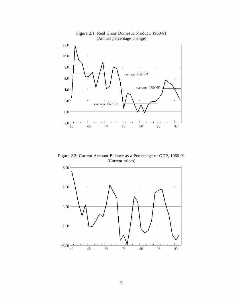
Figure 2.1: Real Gross Domestic Product, 1960-91(Annual percentage change)
Figure 2.2: Current Account Balance as a Percentage of GDP, 1960-91(Current prices)
9
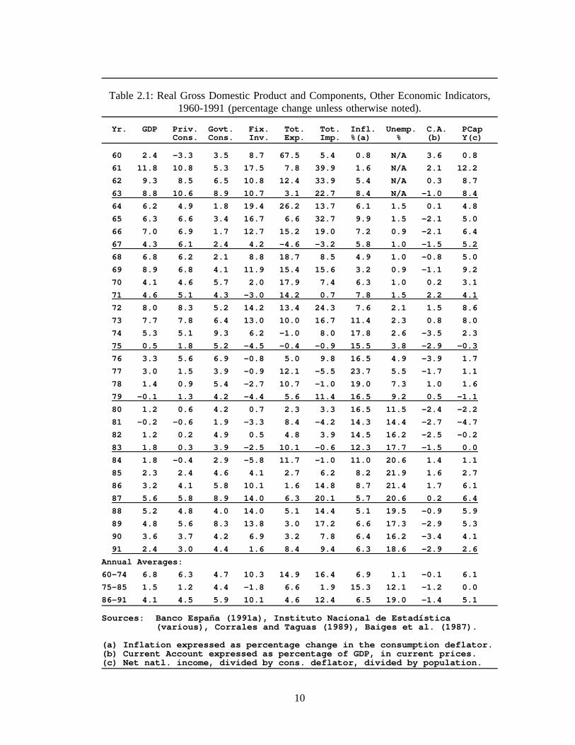
Table 2.1: Real Gross Domestic Product and Components, Other Economic Indicators,1960-1991 (percentage change unless otherwise noted).
Yr. GDP Priv. Govt. Fix. Tot. Tot. Infl. Unemp. C.A. PCapCons. Cons. Inv. Exp. Imp. %(a) % (b) Y(c)
60 2.4 -3.3 3.5 8.7 67.5 5.4 0.8 N/A 3.6 0.8
61 11.8 10.8 5.3 17.5 7.8 39.9 1.6 N/A 2.1 12.2
62 9.3 8.5 6.5 10.8 12.4 33.9 5.4 N/A 0.3 8.7
63 8.8 10.6 8.9 10.7 3.1 22.7 8.4 N/A -1.0 8.4
64 6.2 4.9 1.8 19.4 26.2 13.7 6.1 1.5 0.1 4.8
65 6.3 6.6 3.4 16.7 6.6 32.7 9.9 1.5 -2.1 5.0
66 7.0 6.9 1.7 12.7 15.2 19.0 7.2 0.9 -2.1 6.4
67 4.3 6.1 2.4 4.2 -4.6 -3.2 5.8 1.0 -1.5 5.2
68 6.8 6.2 2.1 8.8 18.7 8.5 4.9 1.0 -0.8 5.0
69 8.9 6.8 4.1 11.9 15.4 15.6 3.2 0.9 -1.1 9.2
70 4.1 4.6 5.7 2.0 17.9 7.4 6.3 1.0 0.2 3.1
71 4.6 5.1 4.3 -3.0 14.2 0.7 7.8 1.5 2.2 4.1
72 8.0 8.3 5.2 14.2 13.4 24.3 7.6 2.1 1.5 8.6
73 7.7 7.8 6.4 13.0 10.0 16.7 11.4 2.3 0.8 8.0
74 5.3 5.1 9.3 6.2 -1.0 8.0 17.8 2.6 -3.5 2.3
75 0.5 1.8 5.2 -4.5 -0.4 -0.9 15.5 3.8 -2.9 -0.3
76 3.3 5.6 6.9 -0.8 5.0 9.8 16.5 4.9 -3.9 1.7
77 3.0 1.5 3.9 -0.9 12.1 -5.5 23.7 5.5 -1.7 1.1
78 1.4 0.9 5.4 -2.7 10.7 -1.0 19.0 7.3 1.0 1.6
79 -0.1 1.3 4.2 -4.4 5.6 11.4 16.5 9.2 0.5 -1.1
80 1.2 0.6 4.2 0.7 2.3 3.3 16.5 11.5 -2.4 -2.2
81 -0.2 -0.6 1.9 -3.3 8.4 -4.2 14.3 14.4 -2.7 -4.7
82 1.2 0.2 4.9 0.5 4.8 3.9 14.5 16.2 -2.5 -0.2
83 1.8 0.3 3.9 -2.5 10.1 -0.6 12.3 17.7 -1.5 0.0
84 1.8 -0.4 2.9 -5.8 11.7 -1.0 11.0 20.6 1.4 1.1
85 2.3 2.4 4.6 4.1 2.7 6.2 8.2 21.9 1.6 2.7
86 3.2 4.1 5.8 10.1 1.6 14.8 8.7 21.4 1.7 6.1
87 5.6 5.8 8.9 14.0 6.3 20.1 5.7 20.6 0.2 6.4
88 5.2 4.8 4.0 14.0 5.1 14.4 5.1 19.5 -0.9 5.9
89 4.8 5.6 8.3 13.8 3.0 17.2 6.6 17.3 -2.9 5.3
90 3.6 3.7 4.2 6.9 3.2 7.8 6.4 16.2 -3.4 4.1
91 2.4 3.0 4.4 1.6 8.4 9.4 6.3 18.6 -2.9 2.6
Annual Averages:
60-74 6.8 6.3 4.7 10.3 14.9 16.4 6.9 1.1 -0.1 6.1
75-85 1.5 1.2 4.4 -1.8 6.6 1.9 15.3 12.1 -1.2 0.0
86-91 4.1 4.5 5.9 10.1 4.6 12.4 6.5 19.0 -1.4 5.1
Sources: Banco España (1991a), Instituto Nacional de Estadística(various), Corrales and Taguas (1989), Baiges et al. (1987).
(a) Inflation expressed as percentage change in the consumption deflator.(b) Current Account expressed as percentage of GDP, in current prices.(c) Net natl. income, divided by cons. deflator, divided by population.
10

partly the result of an increase in foreign investment as transnational firms aspired to
profit from the growing internal market and establish a foothold in the European market.
Since 1986, imports have exploded, but export growth has been disappointing, and a
large trade deficit has evolved. Reasons for this outcome include a higher demand
growth rate in Spain relative to its EC partners, higher inflation and wage growth,
reduction of Spanish trade barriers, and a steady appreciation of the peseta since EC
membership. Also, foreign investors in Spanish production facilities normally import
foreign capital equipment. Accordingly, the substantial inflow of direct foreign
investment since 1985 stimulated a direct flow of imports.
Throughout the modern history of Spain, the trade balance was the major constraint
on the economy. A major stabilization plan was instigated in 1959 as a result of a
foreign exchange crisis brought about by chronic trade deficits. During the growth years
of the sixties, periodic trade imbalances induced restrictive policies by the government.
Large deficits and inflation caused by the oil price shocks of the 1970s repressed growth
for a long period. The resulting "stop-and-go" characteristic of the current account can
be seen clearly in Figure 2.2. Therefore, the present deficit produces uneasiness
surrounding the future of the economy.
The Years of Prosperity: 1960-1974
A high rate of GDP growth from 1960 through 1974 is only part of the story. A
large structural shift from agriculture towards services also characterized this period.
Table 2.2 illustrates the magnitude of this shift. In 1960, the proportion of the GDP
arising from agriculture was 22.3 percent, while industry and services accounted for 28.7
and 43.5 percent, respectively. By 1975, agriculture produced only 9.5 percent of GDP,
11

Table 2.2: Sectoral Proportion of GDP and Employment, 1960-1989.
1960 1965 1970 1975 1980 1985 1990
Value added percentage of current price GDP (a)
Agriculture 22.3 15.5 10.7 9.6 7.1 6.3 4.6Industry 28.7 33.0 32.9 32.3 30.2 30.5 25.6Construction 5.5 7.6 9.1 9.6 8.4 6.5 9.0Services 43.5 41.6 45.2 46.6 52.5 54.8 54.6Import Taxes -- 2.3 2.1 1.9 1.8 2.0 0.7Value Added Tax -- -- -- -- -- -- 5.5GDP 100.0 100.0 100.0 100.0 100.0 100.0 100.0
Percentage of total employment
Agriculture 40.5 35.7 30.5 23.4 18.8 18.2 11.8Industry 23.5 23.5 24.8 26.9 27.2 24.5 23.7Construction 6.7 8.5 9.5 9.6 9.0 7.3 9.7Services 29.2 31.0 33.8 38.6 44.9 50.0 54.8Total 100.0 100.0 100.0 100.0 100.0 100.0 100.0
Sources: Instituto Nacional de Estadística (1988), Banco de España(1991b), Corrales and Taguas (1989), Dehesa et al. (1988).
(a) All figures GDP market prices (including taxes and subsidies) except1960 which is GDP at factor cost (excluding taxes and subsidies.
while industry’s share had climbed to 32.3 percent, and the service share to 46.6 percent.
The agricultural share of total employment fell from 40 to 23 percent. These jobs were
compensated by employment expansion in each of the other three sectors, with services
absorbing the most, increasing its share from 29 to 39 percent. This combination of rapid
growth and structural change allowed Spain to close the gap between itself and the rest of
the industrial world.
The foundations for the development of the Spanish economy in the 1960’s were laid
in the previous decade. The industrialization of the economy had begun in earnest in the
1950’s under the import substitution policies of the Franco regime (Dehesa et al. 1988).
This philosophy was adopted because of a suspicion of free markets held by the government
12

leaders and because of the political isolation of Spain following World War II.1 Economic
policies of this era included price controls, especially on food products, and government
intervention in capital markets to channel investment to favored sectors. An elaborate
system of import licenses, quotas, tariffs, and foreign exchange controls favored industrial
development. This industrial bias induced massive migration of at least one million people
from rural to urban areas. The result was "a growing urban and monetary economy
endowed with an intermediate level of technology and appropriate and flexible human
capital" (Dehesa et al. 1988, p. 10).
Nevertheless, the import-substitution-driven economy ran out of momentum by the late
1950’s, when the economy sustained huge trade-balance deficits. These deficits were driven
by an ever increasing need for imported intermediate and capital goods to feed the growing
domestic industries. Also, the anti-agricultural bias, an over-valued exchange rate, and
protection for domestic industry discouraged exports. By 1959, Spain had run out of foreign
exchange and could not import the foodstuffs, let alone the intermediate and capital goods,
on which it had come to depend. This fact, coupled with inflationary financing of public
sector debt (see below), spurred high rates of inflation (an average of 8.5 percent from 1954
to 1959). Faced with this crisis, the government, in cooperation with the International
Monetary Fund and Organization for Economic Cooperation and Development, adopted the
Stabilization Plan of 1959 (Plan Nacional de Estabilización Económica). This plan was
composed of three elements (Fuentes Quintana 1989):
1) Liberalization of the Foreign Sector. The peseta was devalued and a uniformforeign exchange rate system introduced. A rapid liberalization of importlicense/quota and tariff systems reduced the industrial bias and protectionist
1 It is well known that Spain had always held to a mercantilist philosophy throughoutits history. The economic policies of the early Franco regime were not a deviation from thistradition.
13

nature of the previous system. A new foreign investment law encouragedinflows of capital.
2) Balancing of the government budget and a halting of subsidies to publicenterprises. Taxes and prices for publicly provided goods increased. Becausegovernment debt was financed by securities that were immediately monetizedby the central bank, the reduction of the government deficit reducedinflationary money creation.
3) Limitation of liquidity expansion in the private sector. The ceiling on interestrates was raised, and a limitation was placed on the expansion of privatecredit.
The immediate impact of the Plan was an improvement in the balance of payments and
a severe recession. Within a few years, the new policies had the desired effect of alleviating
the problems of unsustainable trade deficits and inflation. More important, however, was
that the trade liberalization elements of the stabilization plan produced the opportunity for
Spain to share in the general world-wide economic boom during the 1960’s. International
prosperity attracted foreign direct investment, tourism and other exports receipts. It also
stimulated a large emigration of labor to other parts of Europe which kept unemployment
low while increasing transfers from abroad. Though there was some occasional backsliding
toward protectionism, Spain never returned to its long tradition of autarchy.
Returning to Table 2.1, we see the pattern of real economic growth through the 1960-74
period. The rapid real GDP growth on an average annual basis, 6.8 percent, was
accompanied by a substantial inflation rate (6.9 percent, high compared to the international
standards of the time) and very low unemployment (1.1 percent). While government
spending grew at a modest pace of 4.7 percent, the public sector was a net lender to the
economy, mainly because of a surplus in social security. The economy displayed very high
growth rates of fixed investment (10.3 percent) and exports (14.9 percent, including
tourism). The 16.4 percent increase in imports was offset by transfers from Spanish workers
14

abroad to produce a balanced current account, on average. Obviously, the high growth rates
of foreign trade represent a significant change in the degree of openness of the Spanish
economy. The proportion of current price imports to GDP increased from 7.5 percent in
1960 to 19.2 percent by 1974, the export proportion from 10.3 to 14.4 percent.
Nevertheless, other factors prevented a more thorough transformation of the economy
(Dehesa et al. 1988). In 1964, a new round of subsidies, tax exemptions and special
financial privileges, reduced the momentum created by the 1959 reforms. A poor taxation
system impeded complete and fair collection of income and property taxes, leading to a
shortage of public goods and infrastructure investment. The efficiency of the labor market
was hampered by regulations stipulating the duration of labor contracts, restricting dismissals
and mandating levels of severance pay. Trade unions were illegal and there was no right
to strike. Reforms in this area would have run counter to the philosophy of the Franco
regime, which emphasized a paternalistic system of job security in exchange for worker
discipline and low wages (Toharia 1988, p.120). Remnants of this system still impede labor
mobility and economic growth today.
As evident in the stabilization plan outlined above, the government still exercised tight
control in the financial system, imposing interest rate ceilings and barriers to entry for new
lenders. The low, and often negative, rates of real interest insured that credit rationing was
the rule. Since a large proportion of financial resources were channelled to preferred
recipients through compulsory investment rules, the most economically deserving investment
projects lost out to the dubious projects of the well-connected. Exchange controls remained
substantial and tended to isolate the Spanish capital market from the rest of the world.
Politically powerful bankers resisted any suggestion of reform of this system. As we have
seen, inflationary pressures were strong during the period. When the combination of
15

inflation and trade imbalances periodically appeared, the government authorities introduced
demand cutting measures, usually through ad hoc capital constraints, to stabilize the
situation. Such restrictive measures were significant in 1967, 1971 and 1975.
From 1960 to 1974, the economy was opened to world trade and displayed rapid growth
of production, income and investment. However, much remained controlled and regulated.
These structural and institutional rigidities proved disastrous when the first oil shock and
world recession occurred in 1975.
Economic Crisis: 1975-1985
By 1973, imported oil accounted for 68.3 percent of Spain’s energy consumption
(Salmon 1991, p.6). In that year, large increases in the international price of oil stopped the
Spanish economic juggernaut in the water. The balance of payments turned sharply negative
and domestic inflation increased dramatically. By 1975, economic growth fizzled out.
Structural and institutional rigidities, especially those of the labor market, prevented the
economy from responding with any flexibility to the oil price shock. Moreover, the path
and duration of economic crisis in Spain was profoundly influenced by the political turmoil
associated with the death of General Franco in 1975. At that time, Spain embarked on a
perilous transition to democracy. Economic problems often took a backseat to political ones.
Political problems and social demands overwhelmed the first governments of the
political transition. Social peace was partly bought by a permissive monetary policy and
huge rises in monetary wages (política permisiva, Toharia 1988, p. 123). Because of the
tight labor market, real wage increases had exceeded labor productivity increases for years
(Figure 2.3). Until 1975 the differential had been accommodated by a redistribution of
income between wages and profits (Figure 2.4). From 1975 through 1979, however, the
16

permissive monetary policy allowed firms to avoid the redistributive trend by immediately
passing wage increases into prices. Meanwhile, continued restrictions on interest rates led
to negative real interest rates. Companies increased borrowing, stoking the fires of inflation.
This inflation, which peaked at 23.7 percent in 1977, only postponed the problems of the
Spanish economy. Finally, unemployment, previously very low, increased rapidly, reaching
5.5 percent of labor force by 1977. As we shall see, later adjustments aimed at squeezing
inflation out of the economy proved even more damaging to employment.
Following the first democratic elections of 1977, the various political parties agreed to
initiate measures which would begin the difficult process of economic adjustment. These
policies were formalized by the Moncloa Pacts (Los Pactos de la Moncloa). As in 1959, the
reform policies contained in this document stressed restrictive monetary and fiscal policies.
For the first time, however, Spain’s leaders also agreed to begin reforming the labor market.
In 1977, virtually all industrial wages were 100 percent indexed with inflation. The most
important short-run impact of the pacts was made by changing the wage indexation from
actual inflation to a target (or expected) inflation rate set by the government. Also, the
government agreed to decrease social security tax rates. These two provisions helped to
break the inflationary spiral. As shown in Figure 2.3, by 1979 the increase in real wages
fell below productivity growth. For the longer term, the Moncloa pacts contained provisions
for shorter duration and less costly types of temporary job contracts, and for easier and less
costly dismissals. Finally, the government accepted the responsibility to administer a
restructuring program (reconversión industrial) aimed at reducing excess capacity and
employment in several large industrial sectors (Fuentes Quintana 1989, p. 40-41).
17

Figure 2.3: Real Wages and Labor Productivity, 1965-90. (a)(Annual percentage change)
(a) Real wages defined as gross nominal wages (including social security paid byemployer) deflated by GDP deflator, divided by employment. Labor productivitydefined as real GDP divided by employment.
Figure 2.4: Shares of Wages and Profits in Value Added at Factor Cost, 1965-90.(Percent)
18

The stated aim of the government’s industrial conversion policy was to adapt Spanish
industry to the changing international economic environment and increase its competiveness.
Government intervention was felt to be necessary to promote a more orderly and less costly
restructuring than one that might occur from market forces alone. In practice, the policies
cushioned industries from the full impact of the industrial crisis. These measures took
various forms, including: the promotion of mergers, nationalization or new regulation of
monopoly firms, subsidies and debt writeoffs, and government sanctioning of layoffs and
factory shutdowns with training and benefit assistance to the unemployed workers. The
reconversion was especially important for the metals, shipbuilding, electrical, textiles, and
motor vehicle industries.2
From the Moncloa pacts through 1985, an improving political climate allowed for better
economic policy. Money supply growth and inflation gradually abated and the current
account was in surplus by 1984. However, GDP growth was slow (below 2 percent) and
fixed capital investment experienced negative growth in eight of the years from 1975
through 1984 (Table 2.1). Restrictive demand policies and restructuring took an enormous
toll on employment. Figure 2.5 illustrates the magnitude of the job destruction. Between
1974 and 1985, employment was reduced by 2.2 million positions; the unemployment rate
increased from 2.6 percent to a peak of 21.9 percent in the same period. By 1991, it was
still hovering at 16 percent, and remains the major problem of the Spanish economy today.3
2 For detailed descriptions of the reconversion programs, see Salmon (1991, 112-145).
3 The actual unemployment rate remains disputed. Spain has a substantial undergroundeconomy. The proportion of underground to documented activity probably increased duringthe crisis. Moreover, expansion of unemployment compensation eligibility induced entryinto the labor force of unemployed persons who would not otherwise be there. Therefore,it is possible that official employment figures increasingly underestimate the number ofworkers employed. However, a measure of the "real" unemployment, say, five percent belowthe official rate, would still place it among the highest in the EC.
19

Figure 2.5: Employment and the Labor Force, 1964-91.(Millions of persons)
EC Integration and Economic Boom: 1986-1990
Economic membership in the European Community (EC) influenced the Spanish
economy significantly. Growth began at a rapid pace starting in mid-1985, just before Spain
joined the EC. From 1986 through 1990, Spain experienced the most rapid expansion of
the Community, averaging 4.5 percent GDP growth and 4.8 percent private consumption
growth. While the growth of Spanish exports was steady, that of its imports was much
stronger, throwing the current account into a fat deficit. This constraint, however, has been
softened by the large flow of foreign direct investment. Indeed, a large portion of the
increased imports can be directly attributed to the capital inflow, as foreign investors have
imported great quantities of durable equipment (see Section 1.2 and Chapter 6).
The most striking characteristic of this boom was the vigorous expansion of investment.
From 1986 through 1990, investment in machinery and transportation equipment increased
at 15.3 percent, residential construction 5.6 percent, and non-residential construction 15.0
20

percent. Since fixed investment stagnated significantly during the crisis, the renewed growth
represents a needed rebuilding of capital stock, but it also signals a healthy confidence in
the economy by both domestic and foreign agents. It also suggests a recognition by Spanish
producers, whether foreign or domestic, of the need to accumulate the most modern and
productive technology available in order to compete in the European single market which
starts in 1993. Furthermore, helped by EC structural transfer funds and spurred by the 1992
Olympics in Barcelona and the 1992 World Exposition in Seville, government investment
in infrastructure increased substantially. It is hard to drive a car anywhere in Spain without
encountering construction-related delays. We shall examine investment behavior in detail
in Chapter 5.
Since the explosion of foreign direct investment played an important role in the
investment boom, it deserves further explanation. Table 2.3 displays the total and direct net
foreign investment flows into Spain for the period of 1982 through 1990. By 1990, both
figures are almost ten times greater than in 1982. There are several plausible reasons for
this gush of foreign capital, including (Martín 1990a, p.216; Larre and Torres 1991):
1) the reduction of uncertainty surrounding future economic regulation due toSpain’s integration in the EC;
2) the possibility of gaining a foothold in the EC market within a country withlow relative labor costs;
3) the promise of plentiful profits from a domestic market growing faster thanthe EC average;
3) the greater availability and reduction in costs of imported inputs, due to tradeliberalization, which raises the rate of return of capital;
4) the exploitation of Spanish government incentives to foreign investors,especially for activities in certain high technology sectors or regions ofinterest.
21

Table 2.3: Total and Direct Net Foreign Investment into Spain, 1982-90.(Billions of pesetas)
Year Total % change Direct % changeNet Inflow Net Inflow
1982 198.8 -- 111.4 --1983 243.7 22.5 121.5 9.11984 322.1 32.2 156.4 28.51985 412.9 28.2 164.2 5.21986 716.8 73.6 284.2 73.11987 996.5 39.0 321.5 13.11988 1063.5 6.7 521.1 62.11989 1730.1 62.8 667.3 28.11990 1845.5 6.7 1073.1 60.8
Source: Banco de España, Boletín Estadístico (various years).
A very large proportion of the foreign investment has been directed toward industrial
sectors with rapid demand growth, such as pharmaceutical, automobiles, computers,
electronics and food processing (Ministerio de Industria y Energía 1990; Buiges et al. 1990,
p.7). Now, foreign transnational firms dominate several industries. For example, the motor
vehicle industry expanded to become a leading sector of Spanish industrial development;
Spain is now the sixth largest producer of motor vehicles in the world. The industry,
however, is completely owned by foreign producers. Moreover, this same set of industries
contributes disproportionately to exports. Again taking the auto industry as an example, in
1989 five of the leading ten exporters, including the top four, are companies of this industry
(El Pais 1991, p.392). The situation is much the same in chemicals, computer, electronics,
and, increasingly, food processing.
The bad news from the current expansion is an accumulation of foreign debt to finance
the current account, an excruciatingly slow fall in the unemployment rate, and a steady
increase in inflationary pressures with accompanying high interest rates. (Consumer prices
rose 5.4 percent in 1987 to 6.4 percent in 1990, Table 2.1). A recent increase in real wages
above labor productivity growth, after several years of slower growth, has hindered the
22

competiveness of the economy (see Figure 2.3). Also, entry in the European Monetary
System (EMS) in June of 1989, coupled with a restrictive monetary policy and foreign
capital inflow, resulted in a steep appreciation of the peseta to the top of the 6 percent band
with the German Mark. This did not help the current account deficit, which reached a
record 15.7 billion dollars in 1990.
Prospects for the Modern Spanish Economy
The modern Spanish economy was born in a period of autarchy in the 1950’s. It
experienced expansion during the "economic miracle" of the 1960’s and contraction during
the "economic crisis" of the late 1970’s and early 1980’s. During all this time, the
government took an active role in directing the development of the economy, among other
things, protecting it from international competition, allocating investment funds to preferred
sectors, and retaining majority holdings of firms in several key sectors. As Spanish firms
enter the 1990’s they face several challenges. Most importantly will be the emergence, in
1993, of the European single market. This program contemplates the removal of all
remaining barriers to goods, service, capital and labor movements among the EC countries.4
Also pending is a substantial reduction of tariffs and non-tariff trade barriers with third
countries as Spain approaches harmonization with the Common External Tariffs (CET) of
the EC. Table 2.4 shows that remaining trade liberalization is still quite significant.
Competition will also increase in service markets. As already apparent, domestic industries
and institutions will be buffeted by these changes.
4 Chapter 8 covers the EC single market program in detail. For an overview of specificprovisions and implications of "Europe without borders" see Cecchini et al. (1988) andHufbauer (1990).
23

Table 2.4: Program of Trade Liberalization Under Spain’s EC Membership, 1986-93.
A. Industrial products:
1. Gradual tariff rate reduction process from the base rate(approximately 14%) to zero in the case of other EC countries, andfrom the base rate to the (lower) Common External Tariff rate (CETapproximately 4-5%).
2. The time-table for the above tariff reduction is as follows:
% reductionMarch 1st 1986....... 10January 1st 1987....... 12.5
" 1988....... 15" 1989....... 15" 1990....... 12.5" 1991....... 12.5" 1992....... 12.5" 1993....... 10
Total ...... 100
3. Most quantitative restrictions between Spain and the EC can bemaintained only until 1-1-1990. In fact, Spain got rid of manyquantitative restrictions in 1986.
B. Agricultural products:
1. Products originating in any EC country have preference (relative toproducts originating in non-EC countries) in other EC countries.
2. Common Agricultural Policy accepted as of 1986.
3. Gradual tariff rate reduction for agricultural products to becompleted by January 1, 1993. The time-table for fruits, vegetables,and vegetables fats extends to January 1, 1996.
Source: Viñals (1989).
24

At the same time, the European single market produces opportunities previously
unavailable in an inward-looking economy. Unrestricted access to the huge European
market will enable Spanish producers to capitalize on economies of scale, adapt new
production techniques, and reach new customers. Liberalization of capital flows provides
Spanish firms the possibility of tapping new sources of finance and opens new channels for
investment. While this period is not unlike the early 1960’s where there was a great
opening towards the international economy, firms cannot depend on the state to support them
through hard times. The government is now committed to reducing its interference in
microeconomic affairs, and at any rate, its hands are tied by the regulations promulgated by
the EC.
In this respect, it is important to note that government ownership of firms continues to
be significant. Several public sector holding companies or agencies still dominate several
key sectors, including: (1) Instituto Nacional de Hidrocarburos (INH) in petroleum refining;
(2) Instituto Nacional de Industria (INI) in mining, metals, electricity, shipbuilding and
aircraft; (3) Corporación Bancaria de España (CBE) in financial services; (4) Dirección
General del Patrimonio del Estado (DGPE) in tobacco products, retail services, shipping and
other light manufacturing; (5) RENFE in railways; and (6) Dirección General de Correos y
Telecommuncaciones in postal and telecommunication services. While some limited
privatizations have occurred under a general rationalization of these entities, the present
government is not especially committed to widespread privatization. Because of budgetary
considerations, however, government authorities are committed to a substantial reduction of
subsidies to government firms (see below). In the end, the future course of government
influence of the economy through its ownership in these companies will be played out in
the wider arena of EC debates over the appropriate role of public sector ownership.
25

Especially critical will be European Commission and Court rulings over subsides and public
procurement contracts for state-owned industries. While current proposals stipulate that
national governments must treat public sector firms on an equal basis with any other EC
firm, is not clear whether this will occur in practice (The Economist 1991c, pp.16-18).
The current preoccupation of Spanish economic policy makers and observers (including
ordinary citizens) is to increase competiveness vis-a-vis the rest of the European Community.
Many Spaniards feel that with the arrival of a single European market in 1993, the external
imbalance will become unsustainable and another deep retraction will be required. Since
EC trade barriers to many Spanish products were minimal before 1986, integration had little
immediate payoff in increased exports. In the long run, a competiveness strategy must
encompass a resource shift toward sectors where Spain holds a comparative advantage, the
exploitation of scale economies, the development of new products, a greater application of
modern technology and a penetration of new markets. In the shorter run, however, a
reduction of production costs must play a role. While Spain possesses a significant labor
cost advantage relative to EC countries, the differential has eroded recently. One part of a
competiveness strategy, therefore, is to keep wage increases in line with productivity growth.
Another, complementary, objective is "monetary" or "nominal convergence" with the
rest of the EC in preparation for Economic and Monetary Union (EMU - which includes,
among other items, a common currency) sometime in the late 1990’s. Under agreements
made in the recent Maastricht summit, EMU will start in 1997 if a majority of the current
EC members meet the five "convergence criteria" required to join. If a majority is not ready
by 1997, the EMU will be started in 1999 including the members meeting the criteria,
whether they are a majority or not. The convergence criteria are (The Economist 1991a):
26

1) A country’s inflation rate should be no more than 1.5 percent above theaverage of the three EC countries with the lowest inflation rates.
2) Long-term interest rates should be no more than two percentage points higherthan the average of the lowest three.
3) The government budget deficit must be less than three percent of GDP.
4) The public debt must be less than 60 percent of GDP.
5) The national currency must not have been devalued within the last two yearswithin the 2.25 percent narrow band of the exchange rate mechanism (ERM).
As one might guess, in early 1992 the Spanish economy fails to meet four out of five
of the criteria. Its inflation and interest rates were above the EC average, the budget deficit
was 4.4 percent of GDP and the peseta is contained in the wide 6 percent band of the ERM.
However, as illustrated by Table 2.5 Spain is not alone. Only two countries of the twelve,
France and Luxembourg, would have qualified at the end of 1991. Moreover, Spain satisfies
the criterion which could prove the most difficult one for many nations: Spanish public debt
is only 46 percent of GDP. The primary objective targeted by Spanish policy makers is to
bring down the rate of inflation. Low interest rates and exchange rate stability should
follow.
With this objective in mind, the monetary authorities instituted restrictive policies in
mid-1989 which continued through 1990. It was hoped that these policies would bring down
inflation and domestic demand, and, perhaps, encourage potential exporters to focus on
international markets. The measures did dampen the growth of domestic demand in 1990,
especially for residential construction and durables consumption. Their effect on inflation,
however, was less successful. The consequent high interest rates and appreciating peseta
sustained the foreign capital inflow, especially for government and corporate bonds (Fuentes
Quintana 1991). Many firms, now with greater access to international bond markets were
27

Table 2.5: European Community Indicators of Monetary Convergence, Year End 1991.(Underlined figures meet convergence criteria as outlined in text.)
Country Inflation Long-term Budget Public Currencyrate govt. bonds deficit debt stability
% December, 1991 % of GDP, 1991 est satisfied?
France 2.5 8.8 -1.5 47 yes
Luxembourg 2.4 8.1 2.0 7 yes
United Kingdom 3.7 9.7 -1.9 44 no
Denmark 1.8 8.8 -1.7 67 yes
Germany 4.1 8.1 -3.6 46 yes
Belgium 2.8 8.9 -6.4 129 yes
Ireland 3.5 9.3 -4.1 103 yes
Holland 4.8 8.6 -4.4 78 yes
Italy 6.2 14.1 5.4 101 yes
Spain 5.5 11.7 -3.9 46 no
Portugal 9.8 14.1 -5.4 65 no
Greece 17.6 20.8 -17.9 96 no
Source: Economist (December 14, 1991, p.30).
able to sustain their investment purchases by borrowing abroad. The problem was
compounded by the fact that most controls on capital outflows were still in place.
(Substantial deregulation of capital outflows occurred in early 1991.) Therefore, growth in
imports remained strong at 8.1 percent (down, however, from the 17 percent growth of
1989). This episode illustrates the realities faced by government policy makers in the new
world of liberated capital markets, freer trade and pegged exchange rates.
In the battle against inflation, the government has placed a high priority on the restraint
of wage growth. From late 1990 through the first half of 1991, the national government
attempted to conclude a Competitive Pact (Pacto de Competitividad) between itself, the trade
unions and employer organizations. The objective of this pact was to have each party agree
to play its part in restraining inflation. Most important, it would have attempted to restrain
28
the increase in monetary wages so that real wages would have increased in line with
productivity growth. However, in July of 1991 the trade unions withdrew from the
negotiations. As a result, real wages continued to outrace productivity growth, especially
in the non-tradeable sectors such as services.
The ultimate economic goal of Spaniards is to reach the living standards, however
they may be defined, of their northern neighbors. To accomplish this "real convergence"
it is clear that one element is paramount. To reach the goal, productivity of the labor force
must grow faster in Spain than in its richer trading partners. High productivity growth will
boost real income and help bridle the inflation which undermines the country’s
competitiveness. While we will have much more to say on productivity in Chapter 4, some
observations can be made here.
In both the application of modern technology and the availability of infrastructure, Spain
clearly lags behind the rest of the EC. In recent years, however, the high level of
investment narrowed the gap. This is one step on the road to higher productivity growth.
Because of recent slow economic growth and budgetary problems, the government recently
scaled back investment plans for the next several years. The updated plan calls for a steady
level of public investment at five percent of GDP. This figure still produce a historically
high level of public investment. Prospects for private capital formation are more difficult
to judge, but a reasonable estimate would be for steady but slower growth than the 11.7
percent annual average of 1986-89.
While investment increases the productivity of the employed labor force, Spain must
also take measures to increase the utilization of its considerable under and unemployed labor
resources. An important step is to increase further the flexibility of the labor market. To
American eyes, Spanish labor market regulations appear strange indeed. Regulations
29

stipulate that each employee must be covered by a government sanctioned contract. Most
of the current contracts are of indefinite (read permanent) duration. Termination of
indefinite contracts by employers are complicated and costly and, in any event, normally
involve very high levels of severance pay. Such regulations increase the bargaining power
of employees. Moreover, sectoral wage bargaining is highly centralized, affording little
leeway for troubled firms or for firms located in regions with high unemployment to strike
their own deals with labor (Viñals 1989). Nominal wage growth, therefore, has consistently
kept up with inflation, discouraging employment growth in the face high unemployment.
The government’s high reliance on wage taxes for financing growing social security
requirements also pushes up labor costs.
Over the years, the high fixed costs of hiring and firing, and, especially in the 1970’s,
the high rate of growth in real wages, stimulated an over-investment in labor saving capital
goods. In several industries the capital intensity of production processes is excessive given
the relative capital to labor endowments of the economy (Malo de Molina 1990). There
is also ample evidence that the high level of unemployment is further impeding labor
mobility (Viñals 1989). Among Spanish workers there remains a reluctance towards moving
away from their family, who offer security in times of unemployment. Labor mobility has
also been reduced by housing problems in high growth areas where labor demand is most
vigorous.
A more important reform has been taken place in labor market regulation. Every year,
the proportion of workers covered by fixed-term contracts increases. The existence of these
contracts has opened the door for part-time work and employment training programs.
However, little progress has been made in reducing firing costs. The market is still quite
rigid, preventing a greater adsorption of the unemployed labor.
30

The disappointing performance of the economy in 1991 (2.4 percent GDP growth and
6.3 percent consumer inflation, see Table 2.1) raised fears as to whether Spain would reach
the monetary convergence criteria by 1997. This prompted the government to propose a
package of new budgetary and labor market reforms in early 1992. This "Plan de
Convergencia" is quite controversial since it contemplates the reduction of unemployment
benefits and the new effort to reform labor contract laws. The program also gives a general
outline of fiscal plans through 1996, projecting a public deficit of one percent of GDP by
1996. Among other measures to reduce spending, subsidies to publically owned enterprises
will be reduced and the government health system will be reformed. As of this writing
(April 1992), it is not clear whether the plan will pass the Spanish legislature. There is no
question that the plan can contribute to a better long-run performance of the economy.
However, the Spanish economy faces another, more challenging, problem which is not
addressed by the convergence plan.
Perhaps the greatest constraint facing the Spanish economy is the shortage and unequal
distribution of human capital. While industrial and professional positions are filled with
highly skilled workers, there remains a large unskilled segment of the workforce either
unemployed or in low productivity jobs. This dualism has resulted in inflationary pressure
and hindered job creation in the sectors experiencing the highest rates of growth, especially
professional services and high technology manufacturing. The education system is either
unable or unwilling to provide a solution to this problem. Engineering and technical
programs in Spain require up to six years of study and are highly competitive. In 1987-88,
Spanish universities produced only 3,431 engineers, out of 58,812 students enrolled in
engineering programs. Technical schools graduated only 6,166 of the 78,690 students
enrolled (Instituto Nacional de Estadística, 1991a). In contrast, Taiwan, a country with two
31

thirds of the population of Spain, graduates 37,000 engineers and 136,000 technicians per
year (The Economist 1991b, p.18). It is difficult to escape the conclusion that the entrance
requirements for these professions have been designed, at least partly, to exclude
competition. Alas, reform in this area, as in any country, is difficult because such reform
challenges powerful interest groups (see Olson 1982). A more important example is found
in general education. Most affluent Spaniards send their children to private schools.
Therefore, proposals to increase government support to public schools are not widely
supported and the education provided by them is mediocre. However, in the long run,
productivity growth depends critically on an ever increasing quality and more uniform
distribution of human capital.
The pace of change throughout the past 30 years has left some startling contrasts.
Modern electronic factories exist with cottage textile plants of the underground economy.
Modern cosmopolitan cities stand apart from a "population desert" in almost abandoned rural
villages of the interior that have few modern conveniences. The income distribution, never
very equitable in Spain, is characterized by a growing affluence among urban professionals,
and, on the other end of the scale, the poverty of the urban unemployed and rural farmers.
In the middle is an urban majority trying to cope with swiftly increasing rents, property
prices, and taxes. Of course, this description fits many countries. But in 1992, Spain faces
the opportunity to revitalize its economy, reduce social rigidities and close the gap between
itself and its neighbors. The tradeoff facing Spain is to maximize the long run benefits of
the adjustments while minimizing their short run costs.
32

2.2 A Sectoral Description of the Spanish Economy
Since the empirical model outlined in this work is a sectoral description of the Spanish
economy, on many occasions I will refer to characteristics or conditions in individual
industries. Therefore, it is appropriate at the outset to give a general portrait of the different
industries of the Spanish economy. More detailed and specific descriptions can be found
in Salmon (1991). Table 2.6 displays value added and employment shares for each of the
43 sectors of the MIDE model for 1980 and 1987 (the last year of data availability for
detailed sectoral value added). Table 2.7 exhibits sectoral shares of total exports, the export
share of production, the sectoral shares of imports, the share of imports in domestic demand,
and the current price net exports for each MIDE sector which participates in international
trade. These figures are for 1987.
Sector 1: Agriculture, Forestry and Fishing
Despite the decline in its share of economic activity, the Agriculture, forestry and
fishery industries continue to play an important role in the economy. As displayed in Table
2.6, the sector comprised 5.5 percent of value added and 15 percent of employment in 1987.
Of the total 1987 employment of 1.7 million persons, 1.6 worked in agriculture and forestry,
and the remaining .1 in fishing (Instituto Nacional Estadística 1990b). The industry is also
important in external trade, constituting 7.34 percent of total exports (11.76 percent of
output) and 5.14 of imports (9.21 percent of domestic demand) in 1987. In that year, the
industry also displayed a trade surplus of 90 billion pesetas, the first year of surplus since
at least 1970. Major exports are fresh fruit and vegetables, table olives, and cereals.
Imports include feed grains (especially maize), fresh fish, and live animals. Intermediate
sales to the food processing industries (sectors 15-19, including tobacco) account for almost
33

Table 2.6: Percentage Shares of Value Added and Employment for theProduction Sectors of the MIDE Model, 1980 and 1987.
Value Added (a) EmploymentSector 1980 1987 1980 1987
Agriculture, forest. & fish.
Energy2. Coal & radioactive material3. Coke4. Petrol. extract. & refining5. Elect., gas & water utilit.
Manufacturing6. Metal mining & processing7. Nonmetallic minerals & prod.8. Chemicals9. Metal products
10. Industrial & agric. mach.11. Off. mach, computers, instr.12. Electric & electronic equip.13. Motor vehicles & engines14. Other transport equipment15. Meat & other animal products16. Dairy products17. Other food products18. Beverages19. Tobacco products20. Textiles & apparel21. Leather products, shoes22. Wood & wood products23. Paper & publishing24. Rubber & plastic products25. Other manufactured products
Construction
Private services27. Repairs & reconstruction28. Wholesale & retail trade29. Restaurants, cafes & hotels30. Interior transport31. Maritime & air transport32. Transport related services33. Communications34. Banking & insurance
Imputed prod. of banking (b)35. Business services36. Commerc. & resid. rents37. Private education & research38. Private health services39. Recreat., pers. & oth. serv.
Public and domestic services40. Public administration41. Public education services42. Public health services43. Dom. & oth. nonmarket serv.
7.06
4.440.450.051.912.03
25.761.782.142.282.471.250.181.741.840.830.800.411.881.080.442.360.551.211.270.980.27
8.44
41.401.7112.444.072.560.800.911.505.91-3.524.027.310.781.001.91
11.116.291.992.010.82
5.45
5.950.350.132.413.06
24.481.251.752.181.911.040.631.702.060.790.940.422.001.160.631.760.590.881.451.090.25
7.39
43.371.8113.146.782.680.930.911.596.55-6.134.845.910.631.052.68
11.726.242.472.320.69
19.21
1.280.420.020.130.71
25.690.842.031.482.821.070.191.521.361.010.430.232.030.620.103.801.102.161.390.970.55
8.99
32.301.8813.383.943.710.540.650.862.26--1.220.031.000.901.93
12.535.132.371.753.28
15.04
1.190.390.010.110.68
22.980.671.591.292.660.920.251.351.380.760.470.261.970.610.103.320.911.911.310.870.39
8.15
46.892.0514.465.093.630.430.550.982.39--2.410.011.040.882.35
16.366.993.322.433.62
Sources: Instituto Nacional de Estadística (1988, 1990b, 1991a), Author’scompilations.
(a) Percent share of GDP, does not sum to 100 because of import taxes, whichwere 1.79 and 1.64 percent of GDP in 1980 and 87 respectively.
(b) For explanation of this term, see Chapter 4.
34

Table 2.7: Foreign Trade Indicators forProduction Sectors of the MIDE Model, 1987. (a)
Sector
Exp/Tot Exp(%)
Exp/Output(%)
Imp/Tot Imp(%)
Imp/Dom Dem(%)(b)
Net Exp(bil.ptas.)
Agricult., forest. & fish.
Energy2. Coal & radioact. mat.3. Coke4. Petrol. ext. & refining5. Elect., gas & water
Manufacturing6. Metal mining, proc.7. Nonmet. min. & prod.8. Chemicals9. Metal products
10. Indust. & agric. mach.11. Off. mach. & computers12. Elect. material13. Motor vehicles14. Other transp. equip.15. Meat & oth animal prod.16. Dairy products17. Other food products18. Beverages19. Tobacco products20. Textiles and apparel21. Leather products, shoes22. Wood and wood products23. Paper and publishing24. Rubber & plastic prod.25. Oth. manufactured prod.
Private services28. Wholesale and retail30. Interior transport31. Marit. & air transport32. Transport related serv.33. Communications34. Banking and insurance35. Business services39. Recreation, oth. serv.
Tourism
7.34
9.080.040.018.870.16
45.645.362.254.882.173.971.201.946.320.890.200.124.100.710.032.392.730.962.192.700.53
16.153.831.076.161.780.401.341.370.20
21.79
11.76
15.021.001.4626.190.76
14.5016.9513.3218.2510.5332.2415.9210.6422.0510.141.051.6810.996.050.6912.5341.149.7414.2924.4317.25
5.095.364.3366.1530.314.133.515.081.70
--
5.14
25.821.020.0424.680.08
59.706.251.518.182.976.905.406.566.420.601.130.433.310.660.342.690.591.062.571.460.67
6.190.880.010.691.530.160.702.100.12
3.15
9.21
35.2523.124.4851.700.40
19.4020.5310.0828.8614.8447.3247.9730.4323.737.666.246.279.766.099.2414.8914.1011.5117.5115.9822.27
2.181.380.0319.1528.881.852.018.191.17
--
90.3
-673.6-39.4-2.0
-641.39.1
-1455.5-79.935.2
-332.8-44.3-336.7-282.2-334.1-15.61.4
-71.9-26.530.43.0
-32.2-51.9138.3-2.9-25.215.1-12.7
458.3190.172.6301.7-15.89.319.3
-119.70.8
1579.5
Sources: Instituto Nacional de Estadística (1988, 1991a), Dirección General deAduanas, Estadística del Comercio Exterior de España, FundaciónTomillo, Author’s compilations.
(a) Exports are defined as in the input-output table. Therefore, margins ofwholesale/retail trade, transportation and insurance on merchandise areallocated to these sectors, accounting for the relatively high sharesaccorded to these industries. On the other hand, imports of merchandise arecif (cost insurance and freight) and therefore the merchandise importsinclude the margins.
(b) Domestic demand is defined as output minus exports plus imports.
35

60 percent of the domestic demand for agricultural and fishery goods. Taken together, food
processing is the largest manufacturing industry in the country. Therefore, developments
in the agricultural and fishery sector are critical for another 5 to 6 percent of GDP. Most
of rest of the demand is split between private consumption (20 percent) and intermediate
sales to other sectors such as wood products and restaurants (9 percent).
In general, Spanish agricultural productivity is low in relation to other European
community countries. This is the result of many factors, including: (1) a difficult physical
environment in much of central Spain, (2) a relatively low level of capital application, (3)
the persistence of outdated production techniques, (4) an aging and undereducated
workforce, (5) a distorted farm size structure, and (6) a legacy of often arbitrary
government regulation (Salmon 1991, pp.48-59). However, for several products, such as
vegetables and citrus fruits, there are modern production centers thriving along the coasts
of Spain. Moreover, a recent expansion of irrigation has lifted the productivity of parts of
central Spain. Nevertheless, declines in the level of employment, if not value added, will
continue for the indefinite future.
Spanish agricultural production now represents about 12 percent of that of the EC. The
sector has been, and will continue to be, profoundly influenced by Spain’s integration into
the EC. First, a rapidly increasing proportion of agricultural trade has been with the EC.
The share of agriculture imports from the EC increased from 9 percent in 1980 to 29 percent
in 1987 (Fierros 1990, p.72). In 1980, agricultural exports to the EC were already quite
high, accounting for 82.6 percent of the total exports of the sector. In 1987, this proportion
was almost 87 percent. Spanish farmers will remain dependent on the EC for exports as the
remaining trade barriers come down.
Second, the adoption of the EC Common Agriculture Policy (CAP) prompted
36

substantial changes in the regulatory environment. Before the CAP, the state tended to
control markets through agricultural marketing agencies or price controls. Import controls
were also widely used. These forms of intervention were more rigid than the CAP.
However, taken in total, the breadth of the state intervention was less than under the CAP
(Reig 1989, p.159). Now an elaborate system of price supports and export subsidies applies
to most agricultural production. Overall, membership in the CAP should boost the fortunes
of producers of fruit and vegetables, cotton, rice, sunflowers, olives, and grapes for wine.
On the other side of the ledger, producers of dairy products, animals and cereals (besides
rice) will suffer declining domestic market shares (Reig 1989, pp.167-173).
Sectors 2-5: Energy
As evident in Table 2.7, a crucial aspect of the Spanish economy is its reliance on
imports, especially of crude petroleum, to satisfy its domestic energy requirements. This
dependence was a major cause of economic problems in the 1970’s and early 1980’s and
remains a latent threat today. Natural gas imports, already large, will continue to grow as
domestic users discover the utility of this energy source. Domestic energy production
centers around a largely public-sector domestic coal industry, nuclear and hydroelectric
power. Each of these sources faces problems: low quality coal reserves, strong political
opposition to nuclear power stations, and variable precipitation affecting hydroelectric
production. Oil and natural gas production is negligible.
Coal production expanded rapidly in the late 1970’s and early 1980’s as the government
encouraged substitution of coal for oil. Since 1985, production decreased as import
competition, a lower oil price, substitution of electricity for coke in the metal industries and
environmental considerations have made domestic coal less attractive. The cost of domestic
37

coal is high because of low quality coal, geologically difficult conditions, small scale
production and labor unrest (Salmon 1991, p.87). This industry will experience a continued
decline in the coming years.
Oil refining is split between the public-sector Repsol Group (60 percent of capacity),
Cepsa (24 percent; Salmon 1991, 92), Petromed, a subsidiary of British Petroleum, (10
percent) and ERT (6 percent). This present structure is the result of considerable
restructuring and consolidation throughout the 1980’s. Exports of refined products is
significant, comprising 8.87 percent of total exports and 26.19 percent of total production
for 1987 (Table 2.7). An expansion of exports began in the mid 1980’s when domestic
refiners found themselves with excess capacity as domestic consumption leveled off. As
other European nations cut refining capacity (The EC-12 cut refining capacity by 36 percent
in the mid 1980’s, Spain by only 14 percent; Salmon 1991, p.97), Spanish refiners filled the
void.
Before entry into the EC, the marketing of petroleum products was concentrated in the
publically owned domestic monopoly Campsa. However, EC competition policy obliged
Spain to reorganize Campsa in 1984. It is now jointly owned by each of the above refiners,
with shares divided by refining capacity. The government, therefore, still controls the
industry through Repsol. It also sets maximum and minimum prices throughout each stage
of the process, from the crude oil input price, to the price at the gasoline pump (although
there are plans to deregulate some retail prices). EC competition policy has also required
the elimination of barriers to foreign oil companies in the marketing of products. While
Campsa will retain the monopoly over distribution of any oil products made in Spain,
foreign firms are allowed to market imported products. British Petroleum, Agip, Texaco and
Mobil have entered the competition so far. This competition will affect both the refining
38

and marketing segments of the industry.
A large number of regionally based private utilities supply electricity. However, the
state holding company ENDESA (Empresa Nacional de Electricidad) owns a share in several
of these companies. Financial problems originating from over-expansion in capacity plagued
the industry in the early 1980’s, leading to some consolidation in the middle of the decade.
In technical terms, the largest transformation of the industry was a shift away from fuel oil
generating plants to coal (25.5 percent in 1988; Salmon 1991, p.103), nuclear (17.8 percent)
and hydroelectric (46.0 percent) generating plants. Oil and gas fired capacity made up only
12.7 percent of the total in 1988. Aside from opening the door to some foreign investment,
EC integration will probably have little impact in this sector.
Sectors 6-25: Manufacturing
Several characteristics of Spanish manufacturers are relevant in order to project the
future of Spanish industry (Salmon 1991, 112-115; Martín 1990a). In general, Spanish
industries display lower productivity in relation to their counterparts in other EC members,
Japan and the US. Since they have been highly protected over the years, Spanish industrial
firms are primarily orientated to the domestic market. In several cases, such as cement,
glass and agricultural chemicals, there is a very high degree of concentration where firms
enjoy virtual monopoly power. In other areas such as mining, steel, aluminum, shipbuilding
and aircraft, public-sector firms dominate the market. This situation has led to a lack of
innovation and inflated costs of production. On the other hand, the more competitive
industries (clothing, shoes, parts of the food sector, wood and plastic products) are
characterized by small firm and plant size. This small size has limited the ability of firms
to obtain long-term finance, frustrated the exploitation of scale economies and restricted
39

opportunities to diversify into exports. Therefore, the lack of competition in concentrated
industries and the lack of finance for smaller firms has led to the use of technology which
is older and often obsolete compared to that of potential international competitors.
Furthermore, because of labor market regulation and the high costs of firing, overstaffing
is common in Spanish industry. This characteristic is especially common in industries
owned by the central and regional governments where profitability often takes a backseat
to other social objectives.
Secondly, the industrial structure of Spanish industry is weighted toward traditional
industry. Table 2.6 shows that in 1987 a full third manufacturing value added was produced
by the food, textiles, clothing, shoes and wood products industries (Sectors 15-22). Metal
mining and processing, Non-metallic mineral products and Chemicals account for another
20 percent (sectors 6, 7 and 8). These sectors experienced only medium to low demand
growth the past several years and will continue to do so. Evidence does exist that Spanish
industry holds a comparative advantage in generally labor intensive sectors such as clothing,
footwear, and toys within the EC (Martín 1990a). However, these sectors are subject to
strong competition from South-East Asian and Eastern European countries. In the long-run,
this competition could undermine Spanish export penetration into the northern EC countries.
This suggests a strategy for the application of non-cost competiveness measures such as the
specialization of up-market product ranges and strong brand name marketing.
Third, in industries characterized by higher technology and a more rapid growth of
demand, Spain clearly has problems. In machinery sectors, Table 2.7 shows that the recent
investment boom has induced a strong flow of imports (sectors 10-12). Moreover, the share
of machinery imports from the EC has increased substantially since 1985 due to the
reduction of trade barriers (Fierros, 1990). Industries displaying promising performance
40

(automobiles, computers and domestic electrical appliances) are dominated by foreign firms
applying foreign technology. Reduction of import dependence in these high demand growth
sectors will occur, if ever, after several years of a sustained effort in adopting foreign
technology and implementing domestic research and development programs. Eventually,
formation of human capital in foreign owned enterprises may result in a greater presence of
domestically owned and operated firms in these industries.
With these points in mind, I will now make some observations concerning
manufacturing industries of the Spanish economy. Figures 2.6 through 2.20 display the
output (q), domestic demand (dd), import (imp) and export (exp) for each of the
manufacturing sectors of the economy for the years 1970 through 1989. Data for outputs,
exports and imports come form the MIDE model data base, while domestic demand is
defined as output minus exports plus imports. A common pattern of most of the sectors is
rapid growth both in demand and output through the 1960’s and early 70’s, anemic or
negative growth through the crisis of 1975 through 1985. Since 1985 the fortunes of the
industries are mixed.
In the Metallic mining and base metals processing industry (Figure 2.6), rapid demand
contributed to an overbuilding of capacity in the early 1970’s. Actual demand, however, fell
short of the planners’ projections. The industry was one of the first to be subjected to
capacity reduction and mass layoffs under a reconversion program. Nevertheless, output
remained steady as the government subsidized exports (sometimes called "dumping") in
order cushion the effects of readjustments. While this sector is competitive within the EC,
it is subject to strong competition from the NIC’s of Southeast Asia and Brazil. Moreover,
since world demand growth for metal products will continue to be weak, the prospects for
this sector cannot be optimistic. Production and exports have been down from 1985 levels
41

through 1990.
The fortunes of Nonmetallic minerals and products (Figure 2.7) follows closely with its
major consumer, the construction industry. Stagnation in construction for most of the crisis
years led to a sharp decline in domestic demand. Producers were able to buffer the effect
on production by, again, increasing exports. As construction investment has revived,
however, potential exports have been diverted to domestic demand and imports have risen.
In both the Chemical (Figure 2.8) and Metal products industries (Figure 2.9), production
has not been able to keep up with the revived domestic demand and imports have increased
strongly. As in other sectors, exports have stagnated with the increase of domestic demand.
Even higher demand elasticities for imports is evident in the capital equipment sectors
(Figures 2.10 to 2.12). This phenomena is not only evident in recent years, but also in the
early 70s (see especially Figure 2.10). In both periods, investment booms encouraged a
flood of imports. Underdeveloped industries (in the cases of Industrial machinery and
Computers and precision instruments) and the desire of investing firms to obtain modern
foreign-made technology accounts for this trend. In Sector 10, Industrial and agricultural
machinery (Figure 2.10), agricultural machinery makes up most of the relatively high level
of exports. The rapid expansion of Sector 11, Office machines, computers and precision
instruments (Figure 2.11), is mainly due to the opening of an IBM plant in the Valencia
area. Several other computer makers have also been active in Spain.
42
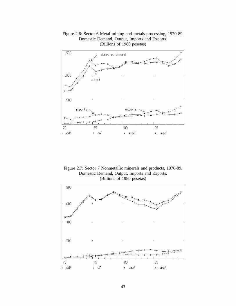
Figure 2.6: Sector 6 Metal mining and metals processing, 1970-89.Domestic Demand, Output, Imports and Exports.
(Billions of 1980 pesetas)
Figure 2.7: Sector 7 Nonmetallic minerals and products, 1970-89.Domestic Demand, Output, Imports and Exports.
(Billions of 1980 pesetas)
43
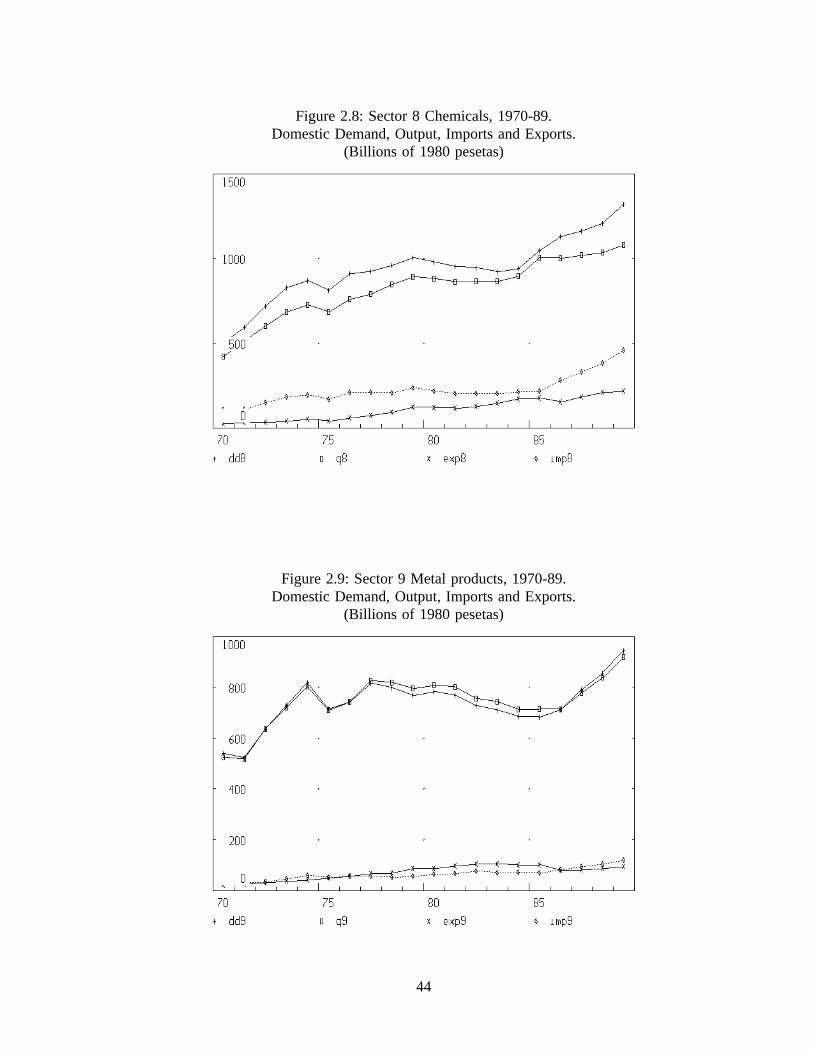
Figure 2.8: Sector 8 Chemicals, 1970-89.Domestic Demand, Output, Imports and Exports.
(Billions of 1980 pesetas)
Figure 2.9: Sector 9 Metal products, 1970-89.Domestic Demand, Output, Imports and Exports.
(Billions of 1980 pesetas)
44

Figure 2.10: Sector 10 Industrial and agricultural machinery, 1970-89.Domestic Demand, Output, Imports and Exports.
(Billions of 1980 pesetas)
Figure 2.11: Sector 11 Office machines, computers and instruments, 1970-89.Domestic Demand, Output, Imports and Exports.
(Billions of 1980 pesetas)
45

Figure 2.12: Sector 12 Electric and electronic equipment and material, 1970-89.Domestic Demand, Output, Imports and Exports.
(Billions of 1980 pesetas)
Domestic demand for, and production of, motor vehicles has been particularly vigorous
since 1983 (Figure 2.13). Registrations of new motor vehicles virtually doubled from 746
thousand in 1985 to 1.4 million in 1988 (Ministerio de Transporte, Turismo y
Comunicaciones 1989). While this demand growth produced a slight trade deficit in the
industry for the years 1987 through 1989, reduced domestic demand starting in 1990 has
probably restored the industry’s traditional trade surplus. At any rate, recent capacity
expansion has provided a modern, competitive motor vehicle industry. As we have noted,
however, this industry is dominated by foreign producers.
The Other transportation equipment sector (Figure 1.13) experienced significant
restructuring during the seventies. Most of the loss of capacity and employment was in the
shipbuilding industry which lost sales because of a general slackening in world demand and
to competitors such as South Korea and Japan. Recently, the shipbuilding industry has been
46

Figure 2.13: Sector 13 Motor vehicles and engines, 1970-89.Domestic Demand, Output, Imports and Exports.
(Billions of 1980 pesetas)
Figure 2.14: Sector 14 Other transportation equipment, 1970-89.Domestic Demand, Output, Imports and Exports.
(Billions of 1980 pesetas)
47

Figure 2.15: Sectors 15-19 Food, beverages and tobacco products, 1970-89.Domestic Demand, Output, Imports and Exports.
Billions of 1980 pesetas.
revived by new demand in the leisure boating market. The public-sector aeronautical firm,
CASA, is part of the Airbus consortium and has enjoyed steadily increased production since
1985. Public procurement contracts have kept manufacturers of railroad equipment working,
but it is unclear whether they can withstand other European competition when bidding for
such contracts must be open to all EC firms.
Figure 2.15 displays aggregated data for the Food processing industries (Sectors 15
through 19: Meat products, Milk products, Other food products, Beverages and Tobacco
products). The graph, however, is not very useful in pointing out several important features
of this huge industry. First, the steady expansion in domestic demand is not so much a
reflection of an increase in the volume of food and drink demanded by Spaniards, but a shift
toward more processed foods, which contain a higher value added component. Moreover,
through time, more food sales are brought under the statistical net as the proportion of
48

informal sales of food products decreases with the urbanization of the society. Secondly,
since the ratios of imports to domestic demand and exports to production are so low, the
graph obscures important changes regarding foreign trade in the sectors. Since 1986, import
penetration increased notably in all the sectors, with the exception of Tobacco products. We
shall have more to say about this in Chapter 5. On the other hand, while exports of wine,
and some dairy and meat products have increased, exports of food products as a whole have
decreased.
Figure 2.16 displays Textiles, clothing, leather products and footwear industries.
Domestic production in these sectors have been highly protected over the years. The sector
required major restructuring to adapt to the decrease in domestic demand during the crisis.
The strong export component of production is evident in the graph. However, exports,
particularly of footwear, were adversely effected by the depreciation of the dollar starting
in late 1985. Integration with the EC has also opened the industry to strong competition
from Italy, Portugal and Greece, as evidenced by the recent surge in imports.
The Wood and wood products industry (Figure 2.17) suffered a prolonged recession due
to a sustained decline in construction and furniture consumption starting in 1980. Recently,
demand has revived. Paper products and publishing - the input-output aggregation in this
sector is unfortunate - (Figure 2.18) did not face a reduction in demand and is presently
enjoying healthy growth. Much the same can be said for Plastic and rubber products and
Other manufactured products (Figure 2.19). These sectors also enjoy buoyant exports (toys
are important), but also have experienced an increasing level of import penetration.
49

Figure 2.16: Sector 20-21 Textiles, clothing, leather products and footwear, 1970-89.Domestic Demand, Output, Imports and Exports.
(Billions of 1980 pesetas.)
Figure 2.17: Sector 22 Wood, wood products and furniture, 1970-89.Domestic Demand, Output, Imports and Exports.
(Billions of 1980 pesetas.)
50

Figure 2.18: Sector 23 Paper, paper products and publishing, 1970-89.Domestic Demand, Output, Imports and Exports.
(Billions of 1980 pesetas.)
Figure 2.19: Sector 24-25 Plastic and rubber products,Other manufactured products 1970-89.
Domestic Demand, Output, Imports and Exports.(Billions of 1980 pesetas.)
51

Figure 2.20: Sector 26 Construction, 1965-90.Proportions of value added in GDP and employment in total employment.
(Percent)
Sector 26: Construction
The industrialization of Spain generated a huge volume of work for the construction
industry. In addition to the job of urbanizing new industrial areas, the provision of
infrastructure for the tourist boom occupied the industry. Over the past thirty years, the
construction industry has been one of the largest sectors of the Spanish economy. Figure
2.20 shows the proportion of GDP and employment contributed by the industry from 1964
through 1990. After rapid growth through the mid-70s, the sector experienced a prolonged
recession throughout the 1975-85 economic crisis. Because of the investment boom of the
late 1980’s, however, the shares in value added and employment returned to 9.58 percent
and 9.7 percent, respectively, by 1990. The construction boom will continue throughout the
early 1990’s, fueled by an enormous demand of public works. These projects include those
associated with the 1992 Olympic games in Barcelona, the World Exposition in Seville in
52

the same year, and the construction of high speed rail links with the rest of Europe. In
addition, while the recent growth of residential housing construction (5.6 percent between
1986-1989) will probably not continue, activity will remain at a very high level. EC
integration will open the construction industry to competition from other European firms,
especially for public works projects, reducing construction prices. In the longer term, it will
force a reorganization and consolidation of a domestic industry made up of many relatively
small companies by European standards (Salmon 1991, p.163).
Sectors 27-39: Private Sector Services
As in any mature economy, the service sector of Spain claims the largest share of value
added and employment. Table 2.6 shows that in 1987 the combined value added and
employment shares for market and nonmarket (mostly government) services are 55 and 63
percent, respectively. However, little research exists on the service industries (sometimes
called the tertiary sector) of Spain. One reason for this is the lack of available data covering
these sectors. No published production or price indices exist for services. For agriculture,
energy and manufacturing, you can count tons of wheat, tons of coal, or number of machines
produced in order to construct such indices. The production of services cannot be similarly
counted. Moreover, the nature and quality of services changes drastically through time. For
example, computerized banking services, such as twenty-four hour banking machines and
debit cards, have increased the accuracy and convenience of banking services. However, if
output is measured by the amount of transactions the total value of those services is
understated. Moreover, the variety of services provided by these industries consistently
expands, and it is difficult to quantify the impact of new services on a historic output series.
Nevertheless, for building an econometrically estimated multisectoral model such as MIDE,
53

it is important to obtain indicators of service output and prices through time. Therefore,
from the beginning of the MIDE project, a special effort has been made in constructing these
series (see Appendix). The result is the most comprehensive data bank on the service
industries of Spain in existence.
The greatest potential impacts of European economic integration lie within the service
industries. The small size of national markets has resulted in a dearth of competition for
these "nontradeable" services. Governments felt that it was necessary to regulate such
industries. Often, intervention consisted of absolute barriers to entry for potential foreign
competitors and the erection of monopolies, usually of the public sector variety. This was
especially true in Spain. Now, the EC Commission is pushing ahead with plans for
integrating and promoting competition in the transport, communications, finance and
business service markets. Moreover, beginning in 1993, the mobility of professionals will
be guided by the "mutual recognition" principle. Under this principle, any professional
licensed to practice in one EC member state must be permitted to practice in all the states.
While several practical obstacles to this ideal must be overcome, it opens the possibility of
German engineers, British lawyers or French doctors setting up business in Spain.
The implications for the Spanish economy of increased competition in services will be
dramatic. Since EC integration in 1986, agricultural and manufacturing industries have been
subject to increasing competition from imports. Up to this point, however, competition in
services has been minimal. This situation is reflected in Table 2.8 which displays the
inflation rate of consumption indices for various good and services. Since 1986, the increase
in the price of services has been consistently larger than the general consumption index and
usually quite larger than the price increases for the categories of food, energy and other
manufactured goods. While there may be many reasons for this dual inflation, the lack of
54

Table 2.8: Inflation Rate for Consumption Price Indices for Type of Products, 1985-90.(percent)
Year General Food Energy Oth. mfg. Serv.(100%) (33%) (7%) (26%) (34%)
1985 8.82 9.52 4.42 9.90 8.131986 8.79 10.64 -6.30 9.85 9.131987 5.25 5.03 -3.92 6.26 6.251988 4.84 3.70 -0.63 4.87 6.821989 6.79 7.67 2.55 3.99 8.671990 6.69 6.51 8.26 4.26 8.57
Note: Figures in parentheses are weight in general index.Source: Instituto Nacional Estadístico, Indices de Precios de Consumo.
competition for providing services plays a large role in the explanation. Not only will
competition in services reduce general inflationary pressures, the quality of the services
provided will surely improve.
The first specific service sector of note is retail and wholesale trade (Sector 28), the
largest single sector of the MIDE model with a 13 percent share of value added and 14
percent share of employment as of 1987 (Table 2.6). The output of this sector consists of
the margins it charges for distribution activities. (In other words, its value added plus the
cost of energy, transportation, office supplies, etc.; but not the costs of goods sold.) The
employment share is significantly higher than in other EC countries (Salmon 1990, 161),
reflecting the nature and relative inefficiency of the industry. Recently, the industry has
been undergoing rapid change. A dual structure of traditional shops and street markets
coexisting with a modern sector of supermarkets, hypermarkets (variety stores) and shopping
centers characterizes the retail system. As consumer patterns (an increasing demand for
more services, such as more convenient hours) and work behavior (married women are
increasing labor force participation very rapidly) change, the traditional sector is losing out
to the modern stores. Accompanying this is increasing concentration, a greater foreign
55

penetration, and the increasing use of modern technologies in both retailing and wholesaling
(Casares et al. 1990). These transformations are resulting in a more efficient distribution
industry.
Spaniards do most of their socializing in bars, cafes and restaurants. Therefore, Spain
has a large, very competitive restaurant sector (Sector 29). The importance of this sector,
which also includes hotels, is also linked with the tourist industry, which we will cover in
detail below. For now, we should note that the sector is not included in Table 2.7 which
presents foreign trade statistics. This is because private consumption in the input-output
table is interior consumption and, therefore, it includes the purchases of tourists made inside
the country. These purchases are not considered exports in the structure of the input-output
table. Nevertheless, the sector is very important in generating exports of tourist services.
Transportation services (Sectors 30-32) are the lubricants of economic activity. Their
most important roles are intra-urban mass transit (subways, busses and intra-urban railroads)
and the facilitation of trade and business exchanges between different regions and nations
(airlines, trucking, inter-regional railroads, and maritime transport). Every other sector of
the economy purchases transportation services. Agriculture, mining, construction, and the
food industries are particularly dependent on transport. It is also important to the tourist
trade. But throughout Europe, and especially in Spain, lack of competition results in a
sticky lubricant. The transport sector is subjected to substantial regulation which is justified
in order to avoid monopoly pricing and negative externalities (e.g., traffic congestion) or for
reason of safety. Regulation of capacity and prices exist for all types of transportation. In
urban mass transportation, railways and airlines, the government owns monopolies providing
the services. In Spain, the small size of the market, lack of competition and poor
infrastructure has led to a very inefficient and costly transportation system even by European
56
standards.
EC integration will have direct influences for highway freight, airline and maritime
transportation industries as barriers to foreign entry to the domestic market will be removed.
More pressure from trucking companies will force nationalized railroads to cut cost to hold
market share. All customs stations will be removed at EC borders, resulting in a gain in
efficiency for highway and airline transportation. One estimate of the savings of eliminating
border controls is $10 billion annually (Cecchini et al. 1988, Table 9.2). Finally, EC
structural funds have afforded Spain the opportunity to make improvements in roads,
railways, subways and airports, all badly needed and overdue. While some Spanish private
and public transportation firms will be harmed and may even disappear with integration,
consumers of transportation services will benefit immensely. For an overview of the future
of transportation policy in the EC see Swann (1988).
Postal services and telecommunications comprise the Communications sector (Sector
33). Demand growth in the industry has averaged almost 10 percent since 1985, the bulk
of the growth in telecommunications services. The high rate of growth will certainly
continue as telecommunications services have become an integral part of the modern
economy. This sector is dominated by the two government monopolies: Dirección General
de Correos in postal services and Telefónica in telecommunications. It does not appear that
these monopolies will experience any substantial competition in their traditional services for
the foreseeable future. However, the possibility exists for competition in new "enhanced"
telecommunications services such as credit card and airline reservation networks (Cowhey
1990).
The banking system (most of Sector 35) of Spain consists of state banks (recently
consolidated into the Corporación Bancaria de España (CBE), now the largest single banking
57
entity in Spain), commercial banks and savings banks. The commercial sector, while being
fairly concentrated, contains several small and inefficient banks by international standards
(Viñals 1989). The private banks have extensive and dense branch networks that add to
fixed costs. However, collectively Spanish banks were the most profitable in the world in
1990 (Economist 1991c, 79). This profitability is the result of wide interest rate margins
as a result of market power, and, until recently, government regulation which sheltered the
industry from both domestic and foreign competition. Moreover, Spanish banks possess
large holdings in other sectors of the economy which allowed them to share in the profits
generated during the recent economic boom. However, profit margins will surely sink with
financial deregulation and more competition among domestic banks and from foreign
entrants. There exists much scope for cost cutting and consolidation within in the industry,
in order to become more competitive in the expanding international market. Moreover, the
banking sector’s ties to the rest of the economy leave it vulnerable to crises which may
occur in individual industries.
Sectors 40-42: Public Sector Services
In the MIDE model, public consumption is grouped into three categories, each one
comprising an individual production sector: Public Administration (Sector 40 - including
central, regional and local governments), Education services (Sector 41) and Health services
(Sector 42). Each of these consumption categories has grown faster than the economy as
a whole since the establishment of a democratic government in the mid-1970s. Three main
factors account for this growth (Viñals 1989, 163):
58
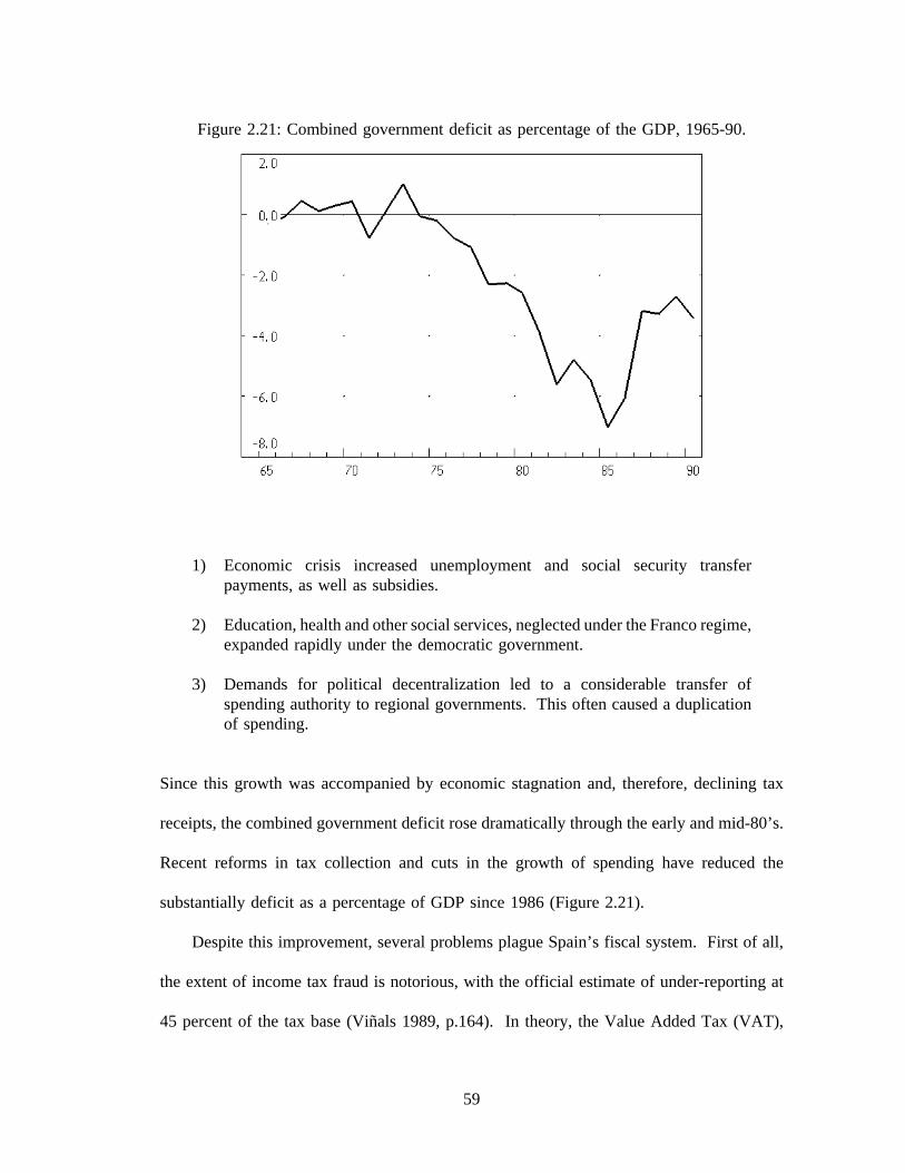
Figure 2.21: Combined government deficit as percentage of the GDP, 1965-90.
1) Economic crisis increased unemployment and social security transferpayments, as well as subsidies.
2) Education, health and other social services, neglected under the Franco regime,expanded rapidly under the democratic government.
3) Demands for political decentralization led to a considerable transfer ofspending authority to regional governments. This often caused a duplicationof spending.
Since this growth was accompanied by economic stagnation and, therefore, declining tax
receipts, the combined government deficit rose dramatically through the early and mid-80’s.
Recent reforms in tax collection and cuts in the growth of spending have reduced the
substantially deficit as a percentage of GDP since 1986 (Figure 2.21).
Despite this improvement, several problems plague Spain’s fiscal system. First of all,
the extent of income tax fraud is notorious, with the official estimate of under-reporting at
45 percent of the tax base (Viñals 1989, p.164). In theory, the Value Added Tax (VAT),
59
introduced in 1986, should be less susceptible to fraud since expenditures are often easier
to trace than incomes. In fact, the extent of VAT fraud is also large, and, apparently,
increasing (OECD 1991, p.101). These problems have created an over-reliance on social
security taxes for financing government expenditures. In 1985, Spain collected 39.4 percent
of its tax revenue in wage taxes, while the EC average burden was 29.7 percent (Viñals
1989, 164). High wage taxes increase the relative price of labor, which reduces international
competiveness and aggravates the unemployment problem. Several commentators have
called for cuts in the social security tax rates to be replaced by increases in the VAT rates.
Another entrenched institutional problem of the fiscal system is the method for
distributing spending and taxing power through the various levels of government (Bel i
Queralt 1991). Local and regional governments account for a little over 30 percent of total
government expenditures. With the exception of the Basque territories, however, they
collect little tax revenue. Most of their financial requirements are met by transfers from the
central government. They also have the authority, within limits, to borrow in order to meet
deficits. Therefore, local politicians determine much of the allocation and amount of
government spending, but are not accountable to the voters for the level of tax rates. This
incentive problem is gradually being corrected by a decentralization of taxing authority.
Tourism
Tourism is Spain’s most important export industry. In 1990, 52 million foreign
residents provided $18.6 billion of foreign exchange. The tourism trade surplus was over
$14 billion (Banco de España, 1991b). Moreover, tourism’s backward linkages provide a
propulsive force for the rest of the economy, especially for the construction, transport, food,
restaurant and hotels sectors.
60

Figure 2.22: Gross Tourism Receipts and Payments, 1960-90.(Billions of 1980 pesetas.)
Figure 2.22 displays real gross receipts from non-resident visitors. Devaluation of the
peseta, the opening to foreign investment initiated by the Stabilization act of 1959, and
increases in disposable income in northwest Europe stimulated rapid growth throughout the
1960’s. Foreign visitors were attracted by the low cost of guaranteed sun and beautiful
beaches. The burgeoning tourist industry engulfed regional economies along the coasts,
transforming small fishing villages into international tourist playgrounds. Unfortunately, the
Spanish planning system was unprepared to handle the sudden tide of development.
Disorderly growth of tourist facilities was not accompanied by sufficient infrastructure
investment. The resulting wild land speculation, congestion and other problems would later
turn investors and tourists away.
With the onset of world recession in 1974, the tourist boom faltered and the receipts
fell sharply until 1977. After a brief recovery, income faltered again in the latter part of the
decade. Real gross receipts did not reach the 1973 level again until 1983. This period of
61

decline prompted restructuring in the industry, included the formation of large hotel groups
and a reduction of labor intensity. After healthy growth through most of the 80’s, income
again started falling in 1989, catching the industry by surprise. A number of factors
contributed to this fall: (1) slower income growth in northwestern Europe (especially
Britain), (2) exceptionally good weather in northwestern Europe, (3) a strong peseta and
domestic inflation. The Spanish industry is concerned that changing consumer tastes, a
deterioration in the image of Spanish tourism, and more competitive destinations such as
Northern Africa, Turkey and Eastern Europe may spell long-term decline for the sector.
Furthermore, an enormous proportion of tourism in Spain is based on the mass package
holiday market where competition is high and value added margins are low. As repeat
tourists become more sophisticated, the demand for these type of holidays will decline.
In confronting these problems, the industry, aided by government, has embarked on
strategies to promote new areas and new forms of tourism in Spain. One strategy is to
promote the cultural and natural treasures of Spain located in the country’s interior. "Up-
market" tourism facilities such as luxury hotels, golf courses and exhibition centers are also
being emphasized. These measures may also help reduce the seasonality of the industry.
Regional governments have taken a more active role in improving the existing coastal
facilities by providing better planning and infrastructure.
Tourism is an important ingredient in the Spanish economy. But as real labor costs
accompany real incomes in their convergence with the rest of the EC, Spain may lose much
of its comparative advantage. Undoubtedly, there is still a strong future for the industry,
especially if it can successfully adapt to changing realities. Nevertheless, as Spain becomes
a more diversified, modern and richer nation, it will not be able to depend as much on its
traditional engine of growth.
62

CHAPTER 3:
EMPIRICAL ECONOMIC MODELS OF THE SPANISH ECONOMY
The following chapters describe a macroeconomic, dynamic, multisectoral model of the
Spanish economy (MIDE). MIDE is a disaggregated, comprehensive simulation and
forecasting model. It combines input-output structure with extensive use of regression
analysis to describe the behavioral characteristics of the economy. When appropriate, the
description will compare and contrast the MIDE model with approaches used by other
existing models of the Spanish economy. Therefore, this chapter presents a brief survey of
some of these models. A recent edition of Situación, a journal published by the Banco
Bilbao Vizcaya (1990), contained articles describing several empirical models of the Spanish
economy, including MIDE. The following discussion will take advantage of this survey by
borrowing from these articles.
Empirical economic models provide a bridge between the realm of pure theory and the
real economic world. While built on the foundation of economic theory, empirical models
can make this theory relevant, or show it to be irrelevant, by attaching real-world places and
numbers to the theories. One advantage of these models is that they force an analyst to
make his assumptions about how the economy operates explicit at each stage of the analysis.
The user can then trace the implications of this particular set of assumptions. Furthermore,
empirical models provide quantitative results for which we can judge the relative
significance of the different assumptions. Often, indirect effects of economic developments
or policy which may be neglected by theory are found to be important when quantitatively
modeled. For these reasons, economists use empirical models to evaluate their thinking
about the workings of an economy.
63
There are several different types of empirical economic models, each type designed to
fill different needs. In this survey of Spanish empirical models, I shall concentrate on
macroeconomic, structural models. The term "macroeconomic" refers to models which
depict the economy as a whole, not just a certain industry, market or institution. Typically,
they consist of an econometrically estimated, multi-equation simulation system for a set of
endogenous variables underlying the right hand side of the Gross domestic product identity:
GDP = C + G + V + X - M
In this equation C represents private consumption, G is government consumption, V is
investment, X is exports and M is imports. The scope and detail of relations between the
variables varies widely among models. The term "structural" implies that the design of the
model is influenced by economic theory. To be more specific, the model builder arranges
the behavioral equations and identities of the model in a causal framework that reflects a
theoretical model of the economy.
3.1 Macroeconometric Models
The first type of model considered can be termed the classical econometric-
macroeconomic, or "macroeconometric", models. These models rely heavily on regression
analysis for determining final demand aggregates, but make little or no use of input-output
tables. Consequently, they normally have little industry detail and no accounting for
intermediate consumption. For example, the sales of steel to the automotive industry, which
is not a part of GDP, is ignored. Therefore, classic macroeconometric models cannot assess
industry level impacts of changes in final demands and also have trouble considering
changes in indirect tax rate changes or commodity price shocks.
These models are usually used in government and academic circles to assess
64

macroeconomic results of macroeconomic policies or shocks. Most forecasters use such
models. There are three well known models of such type in Spain: (1) the Wharton-UAM
(Universidad Autónoma de Madrid) built and maintained by the Centro de Predicción
Económico (CEPREDE) in Madrid, an economic consulting firm; (2) the MOdelo de
Investigación y Simulación de la Economía ESpañola (MOISEES), built by a team in the
General Directorate for Planning of the Ministry of Economics; and (3) two integrated
models, INCOYMOD and HISPANIA/PC built by the Economic Studies Service of the
Banco Bilbao Vizcaya.
The Wharton-UAM (henceforth referred to as UAM) model is the oldest and most
elaborate macroeconometric model of the Spanish economy. The model provides four to
five year forecasts and historical simulations for subscribers of CEPREDE’s services. It is
based on annual data. Construction of the first version of the model began at the
Universidad Autónoma de Madrid in 1978 by the Centro de Predicción L.R. Klein. Formal
collaboration between the its builders and Wharton Econometric Forecasting Associates
(WEFA) was initialized in 1980 (Fernandez and Pulido 1990). The model is now part of
project LINK, an inter-connected set of country models headquartered at the University of
Pennsylvania. The LINK system provides all the international variables of the UAM. The
model is fairly disaggregated, providing, for example, estimations for nine different product
prices, eight different types of exports and imports and three different types of investment.
While there is no input-output accounting or intermediate consumption on the production
side, the model uses fixed input-output coefficients to measure the impacts of intermediate
product prices on the final product deflators. This type of price determination allows the
model to assess the impacts of commodity price fluctuations or indirect tax rate changes on
the final prices. Many aggregate macro-models lack this feature.
65

The MOISEES model was developed to appraise the long-term effects of fiscal policy
measures and to help in the elaboration of the macroeconomic and budgetary projections of
the Ministry of Economics (López Blanco and Taguas 1990). Developed only in the past
five years, MOISEES is a relatively small model, highly aggregated and based on annual
data. Nevertheless, it has two interesting and distinguishing features. First, because of its
roles in simulating the impacts of fiscal policy and planning the government’s budgets,
MOISEES endogenizes government receipts and outflows to a large extent. Especially
important are the effects of changes in aggregate income on non-discretionary transfer
payments and tax receipts.
Second, MOISEES is characterized by its builders as a disequilibrium model (Dirección
General de Planificación 1990). Prices are assumed to be sticky and non-price rationing can
occur. In the short run, the capital-to-labor ratio is assumed fixed. The output equation
summarizing this state of affairs is:
Y = min(YD, YP, YLS)
where Y is output, YD is demand, YP is the maximum output given existing capital stock,
and YLS is the maximum output given a fully employed labor force. If the demand
constraint holds (YD is the minimum), the economy is in a Keynesian regime. If a fully
employed capital stock prevents equilibrium between supply and demand (YP is the
minimum) the economy is said to be in a classical regime. Finally, if the restriction is due
to the unavailability of labor at the going wage rate, the economy is in a repressed inflation
regime. In this case, a rise in prices would reduce demand, transferring it into a different
regime, but prices are prevented from rising for some reason.
At any given time, there will firms in the economy in each regime. To determine total
66

output, a CES aggregator function of the three regimes (based on the work of Lambert 1987)
is used to determine these proportions through time. This function is:
Y (YD ρ YP ρ YS ρ)1ρ
where ρ is an index of the structural friction or uncertainty about demand, capacity and labor
supply. In practice, it depends on a matrix of variances and covariances of the historical
deviations of actual output from the output supposed by each of the regimes. Since in the
forecast period, this parameter cannot be determined, it becomes the central assumption of
the model user. Econometrically estimated functions for labor and capital productivity
determine potential supply (YP and YS); behavioral equations for consumption, government
spending, investment (which feeds back into capital stock), imports and exports determine
potential demand (YD). Rationing of demand or supply occurs in the foreign trade sector,
where the import and export identities are inequalities. Space does not allow us to elaborate
more fully here, details can be found in Dirección General de Planificación (1990).
The Spanish National Statistics Institute does not produce quarterly figures for national
account data such as GDP, consumption and foreign trade. Consequently, all the models of
the Spanish economy are based on annual data. Moreover, since the annual accounts appear
with a three to four month lag, it is difficult for the annual models to integrate the latest
information into their predictions. This situation makes it difficult for government and
business leaders to access short run economic conditions. The Economic Studies Service
at the Banco Bilbao Vizcaya (Servicio de Estudios de BBV) has attempted to remedy this
situation by building INCOYMOD (INdicadores COYuntura MODelo). This model consists
of behavioral equations which project national accounts aggregates employing annualized
figures for indicators published monthly or quarterly. The indicators used include industrial
67

production and price indices and employment (Alcaide and Martínez Aguado, 1990). Since
the indicators are available much sooner, INCOYMOD produces estimates for the current
year national accounts based on actual data. For example, by plugging the annualized
indicators for the first two quarters of a year into the equations, the model produces
estimates for the GDP, private consumption and foreign trade for the current year in July.
Users of the information can then get a feel for the actual economic conditions represented
by the national accounts. The studies service of BBV also has a small annual macro model
of the Spanish economy called HISPANIA/PC. Outputs of INCOYMOD are used to update
the medium run predictions of the HISPANIA in a timely fashion.
3.2 Classic Input-Output Models
Classic input-output models are structured around the input-output tables and its
production or price identities (which will be defined in Chapter 4), but make little or no use
of regression-based behavioral equations. The advantage of these models is that the data
requirements are minimal, consisting of one input-output table. The disaggregation of
classic input-output models is limited by the disaggregation of the published input-output
table. Since these models account for intermediate exchanges, they are useful for assessing
industry level impacts for changes in final demand, indirect tax rates or commodity price
shocks. However, projections are normally made by specifying final demands (consumption,
investment, exports and imports) exogenously. Intermediate consumption, prices and income
are determined with strict identities. Consequently, there is no integration between final
demand and prices or income and no guarantee that there will be economic consistency
among, for example, consumption, prices and income. Moreover, attempts to build
"dynamic" input-output models by endogenizing investment based on the capital equipment
68

"requirements" for future output often leads to severe instability problems (Steenge 1990;
Almon 1966). Therefore, classic input-output models are of limited use for forecasting.
Abadía et al. (1981) constructed the first Spanish model in this category. Their 13
sector model was designed to investigate and project the patterns of production, capital
formation, employment and income distribution. The model contains only real variables,
there are no prices or nominal quantities. Consumption and exports are specified
exogenously. Investment is dependent on future capital requirements and imports depend
on the static import requirements implied by the base input-output table. The classic input-
output equation, based on constant intermediate demand coefficients, computes production.
The model is closed by specifying a balance of trade constraint. Abadía et al. used the
model to project possible growth paths for the Spanish economy from 1975-1985 under
different exogenous assumptions for consumption growth. The exercises were useful for
describing the potential for growth given the initial capital stock and external trade positions
of the economy. The model also provided sectoral breakdowns of production, employment
and income distribution for each of the scenarios. However, there is no attempt to generate
the relative and general price movements of the economy.
On the flip side of the coin is IINDIO (modelo de simulación de la Imposición
INDirecta con técnicas Input-Output). This 17 sector model provides the detailed accounting
for price formation in the economy. IINDIO was used by Lasheras et al. (1989) to examine
the price effects of the change of Spanish indirect tax regime in 1986. Previous to EC entry,
the Spanish indirect tax regime was a cascade tax which fell on all sales, including
intermediate consumption. With EC integration, this system was replaced by a value-added
tax (VAT). Under the VAT, the producer’s tax liability is the difference between the tax
charged on his sales and that paid on his purchases of intermediate goods and services.
69
Unlike the old tax, therefore, indirect taxes paid on intermediate inputs are refunded. In this
way, taxes are collected at each stage of production according to the value added. However,
there are exceptions. Sales of several sectors, such as health and education, are exempt form
the VAT. Since these sectors have no tax liability, they have no way of obtaining a refund
for taxes paid on intermediate purchases. Price and government tax revenue implications
of initiating or changing this system must be examined in an input-output framework since
the tax falls directly on some intermediate input purchases.1 The IINDIO approach was
successful in demonstrating the first round impacts of the tax regime change. However,
since there was no price feedback to final and intermediate demands, indirect effects of tax
changes cannot be estimated. Tax revenue results are especially problematic under such a
limitation.
These two classic input-output models illustrate the utility of constructing empirical
models which include explicit accounting for intermediate demand and inputs. One model
describes the real side of the economy; the other is dedicated to investigation of price
formation. Both models are limited by their inability to integrate the effects of demand and
supply on prices, or vice-versa. Such integration is the object of the following two types
of models.
3.3 Computable General Equilibrium Models
Computable general equilibrium models (CGE) are disaggregated representations of the
economy which use input-output structure for the production side of the economy. Data
1 The issues involved here are complicated and will be dealt with in more detail inChapter 4. For an excellent discussion of the European system of value added taxes and itsimplications for modeling see Bardazzi et al. (1991).
70

requirements are larger than those for classic input-output models since income distributions
to the various sectors of households, government and firms are also considered. However,
the data set used in model construction is usually limited to one year. CGE models also
include sectoral-level production functions and disaggregated demand functions for
consumption, imports, investment, etc. They combine input-output structure and behavioral
functions. Normally, however, behavioral parameters are not estimated with regression
analysis as in econometric models but are deduced from the single year’s set of data or
specified exogenously. In the determination of prices, CGE models assume flexible prices
which move to clear all the markets simultaneously (although some CGE models will
assume some sticky prices, such as in the labor market). The models are used to describe
differences between two equilibrium positions, rather than on a dynamic time path of an
economy. As John Whalley, a pioneer in CGE modeling, notes, that the models
are not forecasting tools built to give an accurate picture of the future time pathof actual economies, but are instead a form of theory with numbers whichgenerates insights rather than precise forecasts (Whalley 1986, p.3).
In other words, CGE models are used to estimate different static equilibriums under
Walrasian general equilibrium theory.
One CGE model has been constructed for the Spanish economy by Kehoe, et al. (1988).
It is based on a social accounting matrix (SAM) constructed from the 1980 input-output
table and national accounts and contains twelve production sectors. It differs from other
CGE models in that it allows for excess supply in the labor market (i.e. unemployment) via
an inflexible wage rate. The model was used to assess the effects of the 1986 tax reform.
The approach could be said to be superior to the IINDIO model because of price feedback
effects on final demand. The model has also been used to assess the impacts of the various
economic changes implied by Spanish integration in the European single market (Polo and
71

Sancho 1989). The results of various market union measures, which we will examine in
Chapter 8, are presented as single figures which summarize the deviation of the base run of
the absence of integration. Since the model is static, there is no definition of the time frame
for which the impacts may occur. Moreover, without a dynamic time path, fluctuations in
economic activity which could occur in the meantime cannot be described. To attain this
type of information, another type of model must be utilized.
3.4 Macroeconomic Multisectoral Models
A final type of model can be described as macroeconomic, dynamic and multisectoral.
This type of model combines all the features of the above models. They are
macroeconomic, since the depict the behavior of the economy as a whole and produce
projections for GDP and its components. They are multisectoral and include input-output
accounting which shows intermediate consumption. They integrate intermediate input prices
with sectoral price formation. In contrast to classic input-output models, however,
macroeconomic multisectoral models connect the production and price sides of the economy
through behavioral equations for final demand which depend on prices and output, and
functions for income which depend on production, employment and other variables.
Furthermore, unlike CGE models, they are dynamic, that is, they produce projections of a
time path of the economy rather than differences between "equilibrium" positions.
Therefore, macroeconomic multisectoral models are more suited for forecasting.
An important feature of a macroeconomic multisectoral is the bottom-up technique. In
this approach, the model works like the actual economy in that the macroeconomic
aggregates are built up from detailed projections at the industry or product level, rather than
72

being estimated and distributed between sectors.2 For example, total capital investment,
total imports and total wage income are not projected directly but are computed as the sum
of their parts: investment by specific industries or goods, imports by production branch, and
labor compensation by industry. The bottom-up technique gives the model the ability to
describe how changes in one industry, such as increasing productivity or changing input-
output coefficients, affect other, related sectors and the general economy. Also, parameters
in the behavioral equations differ between products or industries, reflecting differences in
consumer preferences, price elasticities in foreign trade, and industrial structure. Finally, the
detailed level of disaggregation permits the modeling of prices by industry, allowing one to
explore the causes of relative price changes, and their effects on industry output, structure,
and employment.
In 1981, the European Commission sponsored the HERMES (Harmonized European
Research Macrosectoral Energy System) project for building and linking a collection of
macroeconomic, multisectoral models for the EC countries. The specification for each of
the models is homogeneous, based on the document "European Project for a Multinational
Macrosectoral Model" by d’Alcantara and Italianer (1982). A significant study developed
from the entire HERMES system is Catinat and Italianer (1988). This study provided the
quantitative macroeconomic impacts of the European single market presented in the now
famous Cecchini report (Cecchini et al. 1988) sponsored by the EC Commission.
Unfortunately, a Spanish representative of the project was not finished in time for the
project. Consequently, the various studies concerning European integration have very little
2 This is in contrast to another type of multisectoral model which allocatesmacroeconomic model results to sectors through the use of an input-output table. In thistop-down type of model, there is little of no behavioral modeling at the sectoral level. Sinceno such model exists for Spain, the type is not discussed here.
73

to say concerning the Spanish economy (see, for example, Catinat et al. 1988). However,
the HERMES-ESPAÑA model is presently being built and operated by a team at the
aforementioned Centro de Predicción L.R. Klein at the Universidad Autónoma de Madrid.
A survey of the model is found in Dones Tacero et al. (1990).
HERMES-ESPAÑA contains nine production sectors, fourteen consumption categories
and five sets of bilateral trade equations. It also includes an energy block to provide a
detailed treatment of eight different types of energy products. The major feature of the
model is the use of sectoral CES (Constant Elasticity of Substitution) production functions
to determine demands for capital, employment and energy. The model is quite complicated,
and it is beyond the scope of this chapter to explain it in detail. Instead, since HERMES-
ESPAÑA is the Spanish model most similar to the model presented here, a brief comparison
of its characteristics to those of the MIDE model can be made.
Two distinctions can be identified. First, while taking similar approaches to modeling
the economy, the MIDE model contains substantially higher degrees of disaggregation (43
production sectors, 43 categories of consumption and 11 types of investment). The
advantages of higher disaggregation are those normally cited in the literature: a richer
depiction of the structure of the economy and more accurate description of economic
behavior. More important, highly disaggregated forecasting models are much more useful
to a business planner because they provide specific information concerning the customer,
supplier, and the own industries of a business. Second, the Spanish implementors of Hermes
were given no room for adapting its structures or equation specifications to Spain. In
building the MIDE model, however, I had virtually unrestricted scope for adapting the model
structure and equation forms to the situation existing in the Spanish economy.
On the other hand, the greater the disaggregation of the model, the greater is the
74

complexity of the model and the greater are the limitations of published data. Also, it is
generally true that the smaller a sector, the more difficult it is to prepare behavioral
equations for the variables of that sector. This is because individual sectoral peculiarities
become more important as the sector modelled becomes smaller. This characteristic,
however, while making life miserable for the modeler, is precisely a point in favor for
greater disaggregation. Nevertheless, data limitations and sectoral peculiarities often lead
to ad hoc specifications in a highly disaggregated model. The trade off is that while these
specifications may not be as grounded in economic theory as we desire, they are grounded
firmly in reality.
75

CHAPTER 4:
GENERAL EQUILIBRIUM FRAMEWORK OF THE MIDE MODEL
The foundation of the MIDE model is a 43 sector input-output table embedded in the
structure of the Spanish national accounts. The data base of the model has been compiled
using the 1980 input-output table and the national accounts published by the Instituto
Nacional de Estadística (INE), and various other sources. It contains annual time series for
sectoral level and macroeconomic variables covering the years 1964 through 1989 (up to
1991 for many variables). The Appendix contains an enumeration of sector and commodity
categories of the model and describes the construction of the data base in detail.
Figure 4.1 illustrates the input-output structure of MIDE. In the table, the quantities
across each row represent the sales of each sector to the different sources of demand. The
top left section of Figure 4.1 is the intermediate demand matrix. This matrix lists the sales
of the product in row i to the industries in column j (qi,j). These intermediate inputs are not
included in Gross Domestic Product (GDP), but nevertheless make up part of the total
demand of the row sectors. To the right of the intermediate matrix appear the final demand
(fi,k) categories which comprise GDP. The final demand components of MIDE are private
consumption, government consumption, investment, change in inventory, exports, and
imports. Imports enter as negative quantities. Each row of the table is summed to give total
demand of the product sector (qi).
Quantities listed down the column for each of the production branches in the A matrix
are the payments to the factors of production. Below the intermediate demand matrix is the
value added, or income, paid to the primary factors of labor and capital and to the
76

Figure 4.1:Input-Output Accounting Framework for the MIDE Model
S D E M A N D GDP ComponentsUP Intermediate Private Govt. Fixed InventoryP consumption for Consump. Consump. Invest. Change Exports Imports Transfers OutputL production (c) (g) (i) (v) (x) (m) (tr) (q)Y
Sector: 1................43 1......43 1......11 q =1. A matrix C matrix B matrix Aq +. Cc +. g +. (natl. (natl. Bi +. accts. accts. v +. goods) goods) x -. m -. tr43
Total Inter. Cons. Total Final Demand
Wages and Salaries TPrimary oinputs Gross Profits t.
(Value Indirect Taxes - I Gross Domestic Productadded) Subsidies n
cImport Taxes o
mValue Added Tax e
Total Inputs Gross Output

government. Three types of taxes are computed in the model. Indirect production taxes
minus subsidies, import taxes, and value added taxes. This income is aggregated to GDP.
The total inputs to each sector, both intermediate and primary, are added down the column
to equal to the output of that sector. A matrix of intermediate demand coefficients, the A
matrix, is constructed with the equation:
ai,j = qi,j / qj ,
where qi,j is the intermediate input flow of product i to industry j, and qj is the output of
industry j.
The input-output table published by Instituto Nacional de Estadística is a product-to-
activity table. It reflects the way the data was collected. Survey data on consumption of
different products is collected from individual establishments, or, in some cases, parts of
establishments. Each establishment (or in the words of the Standard European Accounts,
"homogenous output unit") is classified under an activity which best reflects its principle
product. The establishment is then assigned to the column of the input-output table
corresponding to the activity. The establishment’s consumption of different types of
products is then entered in the appropriate product rows of the activity column. The final
table is the imputed aggregation of each cell entry from the survey data. The column sum
for each activity appears under the heading of effective production. Since it is the sum of
inputs, this total represents the gross production from the units of production.
While an activity is classified under its primary product, it is possible that it also
produces by-products or secondary products which belong in a different classification.
Therefore, the effective production of an activity can contain the output of products which
are classified under different product category in the rows of the input-output table. Since
78

the row sums of the input-output table represent demands by products, there are
discrepancies in the corresponding row and column sums of the table. To reconcile these
inconsistencies, the table is published with a row of transfers added to the bottom of the
table. These transfers sum across the row to zero. A transfer entry in a column represents
the output produced by another industry which is classified as a product of that column
classification, less the by-products or secondary products produced by that column industry.
The transfers are added to effective production to yield distributed production for each
activity, which is equal to the row demand for each corresponding product.
This method introduces certain problems. Ideally, the MIDE model should contain a
product-to-product table. In such a table, the A matrix flows reflect the purchases of
intermediate products for the manufacture of products, rather than for the outputs of
activities. The row of transfers disappears. Unfortunately, there is no information on the
manufacture of secondary and by-products by activity to transform the 1980 published table.
Moreover, the national accounts data on value added and effective production are always
published for activities, not for product categories. For these reasons, I have elected to
simply balance the table by converting the transfers into a final demand column, entering
negatively, as shown in Figure 4.1. Therefore, the output solutions in the MIDE model are
activity-level effective production and can be directly compared with the data in the national
accounts. Since there is no information on the magnitude of the transfers in any other year
except 1980, they are projected in each year as the constant 1980 proportion of effective
production and scaled to sum to zero. While this solution is not ideal, the magnitude of the
transfers is small. If there were significant problems introduced by this scheme, they would
show up in the solutions for output in the historical simulations of the model. I have not
encountered such problems.
79

From this input-output accounting system, a detailed annual simulation model is built
using econometric techniques. MIDE consists of three inter-related submodels: the
production block, the price-income block, and the accountant. The production block
determines constant-price sectoral final demands, intermediate consumption, outputs, labor
productivity and employment. The price-income block computes nominal wages, profits,
net taxes and price indices for each industry. The accountant transforms the sum of sectoral
income into national income and other aggregates with the use of macroeconomic identities
and behavioral equations. It then distributes this income to households, corporations and
government. The model is closed by specifying relationships between the variables of the
production, price-income and accountant blocks. For example, private consumption is
dependent on the prices and income generated by the price-income block, and sectoral wages
are dependent on productivity and employment.
The model uses an iterative solution process, which is displayed in Figure 4.2. In any
given year, MIDE begins in the production block at the upper right hand corner of Figure
4.2 and proceeds counter-clockwise. On the first iteration for a given year, the model
estimates the variables exogenous to the production block such as prices and income (usually
the last period quantities adjusted by a growth factor). These quantities are used to compute
first estimates for the endogenous variables for final demand. The model continues through
the loop, computing each of the interdependent quantities of output, productivity,
employment, value added, prices and income. On subsequent iterations of the full model
in the same year, the computed estimates determined by the rest of the model are used
throughout. The model iterates through this loop until the convergence criteria is met. Each
of these blocks is discussed in more detail below, providing a outline of the interrelation
between the model’s variables. In the interest of simplicity, details on the functional forms
80
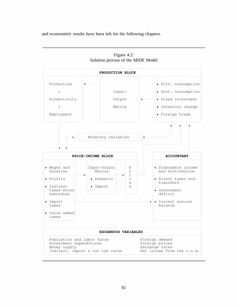
and econometric results have been left for the following chapters.
Figure 4.2:Solution process of the MIDE Model
PRODUCTION BLOCK
Production • Priv. consumption
↓ Input- • Govt. consumption
Productivity Output • Fixed investment
↓ Matrix • Inventory change
Employment • Foreign trade
Monetary variables
PRICE-INCOME BLOCK ACCOUNTANT
• Wages and Input-Output P • Disposable incomeSalaries Matrix r and distribution
i• Profits • Domestic c • Direct taxes and
e transfers• Indirect • Import s
taxes minus • Governmentsubsidies deficit
• Import • Current accounttaxes balance
• Value addedtaxes
EXOGENOUS VARIABLES
Population and labor force Foreign demandGovernment expenditures Foreign pricesMoney supply Exchange ratesIndirect, import & vat tax rates Net income from the r.o.w.
81

4.1 The Production Block
The MIDE model is Keynesian in the sense that the sectoral demands for goods and
services determine the production level. The production block begins by specifying
Government consumption exogenously for three different rows, which correspond to the
classification of the government production sectors of the input-output matrix, Public
administration, Health care, and Education. Intermediate consumption by the government
is allocated to the branches of activity via the input-output coefficients of the government
sectors.
Private consumption is the next order of business. A two-staged process determines:
1) the allocation of private income between consumption and savings, and 2) the allocation
of consumption between 43 categories of goods and services. Additionally, imports and
exports of tourism are computed as an intermediate step in this portion of the model. In the
first stage, a behavioral equation computes aggregate National private consumption. This
approach is perhaps an exception to the bottom-up technique used in the rest of the model.
However, the assumption that consumers decide how to divide their income between savings
and consumption and then decide on which products to consume is not far from reality. At
any rate, the consumption-savings decision is difficult to model on a disaggregated level.
Since consumption comprises 60 to 70 percent of GDP in any one year, it is the most
important quantity in the model. A single-equation representation of aggregate consumption
simplifies the interpretation of the entire model.
Aggregate consumption in the MIDE model depends on household disposable income, a
measure of wealth, the unemployment rate and the interest rate. Real disposable income
enters the equation with a distributed lag, indicating that increases in income do not translate
immediately into a equal increase in consumption, but are partly absorbed by savings (the
82

permanent income effect). Inflation affects consumption negatively through the real wealth
term. Since it tends to devalue their stock of wealth, high inflation motivates consumers
to increase savings in order to maintain their asset stock.
After aggregate national consumption is computed, behavioral equations calculate
Interior consumption by nonresidents and Exterior consumption by residents. The former
is added and the latter subtracted from national consumption to yield total Private interior
consumption. Then, this total is distributed among 43 categories of goods with a nonlinear
econometric system of per capita consumption functions. Demand for each good depends
on per capita real aggregate interior consumption expenditures, the one period difference in
real per capita aggregate expenditures, a time trend to reflect changing tastes or
demographics, its own price, and the prices of all the other goods. Since the commodities
do not correspond with the production branches, the projections from these equations are
converted to private interior consumption expenditures by industry via a share or bridge
matrix.
Most multi-sectoral models contain investment equations by purchasing sector based
on neoclassical production functions where investment is derived from the demand for
capital as a factor of production. Unfortunately, sufficient data on capital stocks and
investment purchases by sector do not exist for the Spanish economy. Therefore, the MIDE
model uses a specification found more often in macroeconomic models, an accelerator
equation which estimates demand for capital by product (industrial machinery, office
machinery, motor vehicles, non-residential construction, etc.).
The traditional accelerator model of investment distinguishes between net investment
and replacement investment. Positive (negative) net investment in a period is defined as the
portion of gross investment above (below) the amount required to replace the depreciation
83

of the capital stock in the period. An accelerator function treats net investment as dependent
on the lagged changes in output of the purchasers of the capital. Adding a replacement
investment term converts the equation into a gross investment function. The equations in
MIDE also contain the ratio of the price index for the capital goods over the price of the
purchaser’s output and the current and lagged ratio of M2 to nominal GDP as explanatory
variables.
The construction of weighted indices for the changes in output and the producer prices
of the purchasing sectors requires some knowledge of the purchasers of each type of
equipment. For this information, I have used a series of capital flow matrices, covering the
years 1980 through 1983, constructed by Antón and Escribano (1988). These matrices show
the flows of investment sales of the type of good to the purchasers, classified according to
the 40 non-government sectors of the 1980 IO table.1 Gross investment in fixed capital is
estimated in this way for nine categories of equipment purchases and non-residential
construction. Residential construction is estimated as a function of disposable income, the
consumption of housing, and the ratio of M2 to nominal GDP. A share matrix distributes
investment goods margins to the service sectors such as retail trade and transportation.
Inventory investment is a small but volatile component of final demand. For some
industries, such as agriculture and petroleum, it can be important. Inventory change for each
of the manufacturing industries is predicted as a partial adjustment to a desired stock. The
stock depends on the level of output.
Foreign trade in the MIDE model is linked to other, similar models through the
1 This information is precisely what is required to construct conventional, neoclassicalinvestment demand equations by purchaser. However, since this study includes only 4observations, the data is still inadequate for this purpose. I await further releases of similardata.
84

INFORUM international trade model (Nyhus 1991). Countries included in this system
include the U.S., Japan, and major European economies. Through this system, sectoral
exports and imports of the Spanish economy respond to sectoral level demand and price
variables projected by models of its trading partners. For example, Spanish merchandise
exports for 25 industries are computed by nonlinear functions which relate exports to the
foreign demand and the ratio of Spanish prices to the foreign prices of that sector. The
domestic production deflators are used to project the export prices for the forecast period.
Both the foreign demands and competing exporters prices come from the INFORUM
international system. The foreign demands are computed by weighting the sectoral imports
of each trading partner by its sectoral share of Spanish exports for 1987. The international
prices are the sectoral production prices of the competing countries weighted by the
participation of each country’s exports in the world market, adjusted by exchange rates.
Transportation and wholesale trade exports consist mostly of margins earned in shipping
and marketing merchandise exports. Therefore, exports for these sectors depend on the level
of merchandise exports. Exports of communications, finance, business and other services
depend on the general level of demand in other European nations as projected by the
INFORUM models. To complete the export accounting, the Interior consumption by non-
residents is added to the merchandise and service exports.
Imports are measured to include the cost of insurance and freight, but not to include
customs duties. Imports for each of the 33 importing branches are projected by nonlinear
equations using internal demand and the import purchaser price to domestic price ratio as
explanatory variables. For the forecast, import prices at the border are moved with the
sectoral production prices of the supplying countries, weighted by the shares of each country
in supplying that commodity to Spain in a base year, and adjusted by exchange rates. The
85

production prices of the trade partners also come from the INFORUM international system
of linked models. Purchaser prices are computed by adding the ad-valorem import taxes to
the border prices. Finally, to determine aggregate imports, Exterior consumption by
residents is added to the sum of the sectoral projections.
Once the final demands are determined they are added to construct the vector, f, of total
final demand for each of the production branches. The formation of f is done by the matrix
equation:
f = Cc + g + Bi + v + x - m - t
where: C = the 43x43 consumption bridge matrix,c = the 43x1 vector of private interior consumption by commodity,g = the 43x1 government consumption vector,B = the 43x11 investment bridge matrix,i = the 11x1 gross investment vector,v = the 43x1 inventory change vector,x = the 43x1 export vector,m = the 43x1 import vector,t = the 43x1 transfer vector.
Sectoral output is then computed by use of the Leontief equation:
q = Aq + f
where: q = vector of constant price sectoral outputs,A = intermediate demand matrix, where each coefficient,
aij, of the matrix gives the total constant-price amountof good i needed to produce a unit of good j,
f = vector of constant price final demands.
Since several demand components (i.e. investment, exports, imports, inventories and
transfers) depend on output or domestic demand, they must be computed simultaneously
with output. Therefore, a Seidel iterative loop exists within the production block so that the
solutions for these quantities are consistent.
86
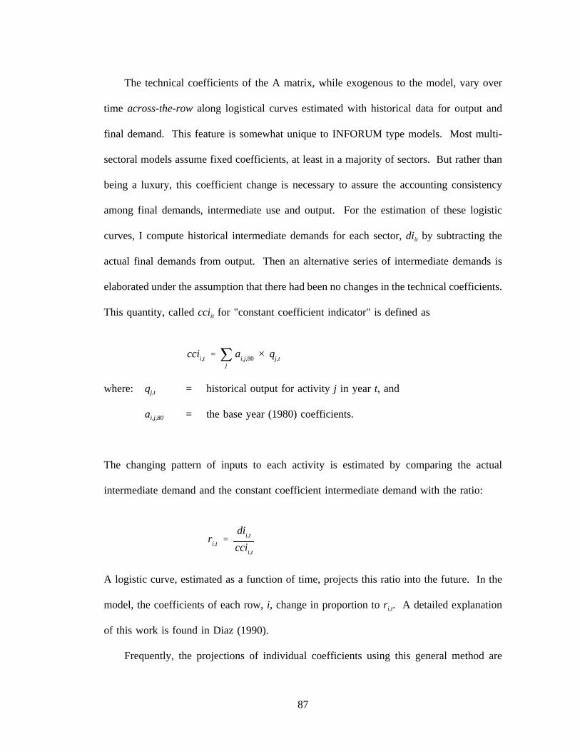
The technical coefficients of the A matrix, while exogenous to the model, vary over
time across-the-row along logistical curves estimated with historical data for output and
final demand. This feature is somewhat unique to INFORUM type models. Most multi-
sectoral models assume fixed coefficients, at least in a majority of sectors. But rather than
being a luxury, this coefficient change is necessary to assure the accounting consistency
among final demands, intermediate use and output. For the estimation of these logistic
curves, I compute historical intermediate demands for each sector, diit by subtracting the
actual final demands from output. Then an alternative series of intermediate demands is
elaborated under the assumption that there had been no changes in the technical coefficients.
This quantity, called cciit for "constant coefficient indicator" is defined as
ccii,tj
ai,j,80 × qj,t
where: qj,t = historical output for activity j in year t, and
ai,j,80 = the base year (1980) coefficients.
The changing pattern of inputs to each activity is estimated by comparing the actual
intermediate demand and the constant coefficient intermediate demand with the ratio:
ri,t
dii,t
ccii,t
A logistic curve, estimated as a function of time, projects this ratio into the future. In the
model, the coefficients of each row, i, change in proportion to ri,t. A detailed explanation
of this work is found in Diaz (1990).
Frequently, the projections of individual coefficients using this general method are
87

unsatisfactory given other available information. In such cases, this information is used to
modify the across-the-row coefficient projections. One example of such a modification is
for the Coal and lignite industry. After the petroleum price shocks of the 1970s, Spanish
government policy strongly encouraged the substitution of coal for oil by controlling coal
prices and subsidizing conversion to coal of large energy users such as power plants, metal
furnaces, ceramic and cement plants (Salmon 1991, p.89). Therefore, intermediate demand
for coal expanded rapidly and this is clearly illustrated by the computed intermediate
demand ratio (ri,t). The projection of this ratio indicates a continuation of this trend. Since
1985, however, demand has stagnated as a lower oil price, substitution of electricity for coke
in the metal industries, and environmental considerations have made coal less attractive.
Moreover, the cost of domestic coal is high because of low quality coal, geologically
difficult conditions, small scale production and labor unrest. The industry, therefore, is
expected to experience a decline in the coming years. In line with this expectation, the
projection its intermediate coefficients shows a slight decline throughout the forecast
horizon.
After the level of production in each branch is determined, labor productivity and
employment per sector is projected. The sectoral productivity variables, defined as output
per hour of labor time, are estimated using regression equations which include exogenous
exponential changes over time and cyclical output fluctuations as independent variables.
Sectoral employment in total hours is related to output by dividing output by productivity.
A second equation for each sector estimates the work year, in total hours per employee, as
a function of time and the change in output. This quantity is divided by the hours of
worked to determine the employment in persons for each sector. For the government
administrative sector, productivity and employment are exogenous. The model computes
88

total unemployment as the difference between the exogenous labor supply and aggregated
employment.
These variables become important factors in other parts of the model. Labor
productivity and employment play key roles in determining the underlying industrial
structure and the growth potential of the economy as a whole. As we shall see below, they
are important inputs for determining the levels of wages and prices. If labor productivity
in a certain sector increases at a rate high enough to decrease the unit labor costs in that
sector, the relative price of its product will fall and demand for the product will increase.
Moreover, total employment (via the unemployment rate) enters into the aggregate wage
index equation. In this equation, productivity growth decreases wage pressure because it
reduces labor requirements. This reduction in inflationary pressures increases real income
and aggregate demand, encouraging faster growth in the economy as a whole. Therefore,
as in the actual economy, productivity growth and its effect on employment play a key role
for determining real economic growth in the model.
Table 4.1 summarizes the discussion of the product block. It shows influences included
in the behavioral equations and identities used for the determination of each product block
variable.
89

Table 4.1: Components and Influences of the Production Block
Variable No. eqs. Influences
Government consumption 3 Exogenous
National private consumption 1 Real wealthReal disposable incomeUnemployment rateChange in the nominal interest rate
Interior consumption 1 GNPs Germany and the UKby foreign residents ER adjusted relative consumption price
of Spain to Germany and the UK
Exterior consumption by residents 1 Real disposable incomeER adjusted relative consumption price
of Spain to Germany and UK
Private interior consumption 43 Total interior consumptionby type of commodity Change in interior consumption
TimeRelative pricesInterest rates
Investment in equipment and 10 Change in purchasing sector outputsnon-residential structures Relative prices of investment goodsby type of investment good Equipment depreciation
Ratio of M2 to nominal GDP
Residential construction 1 Disposable incomeConsumption of housingRatio of M2 to nominal GDP
Inventory investment 25 Sectoral output
Merchandise Exports (fob) 25 Foreign demand by sectorDomestic/foreign sector pricesExchange ratesChanges in domestic demand
Service Exports 8 Merchandise exportsGeneral demand in Europe
90

Table 4.1 : Components and influences of the Production Block (cont.)
Variable No. eqs. Influences
Imports (cif) 33 Domestic demand by sectorForeign/domestic sector pricesExchange rates
Output 43 Intermediate demand + final demand
Labor productivity 42 TimeOutput cycles by sector
Average employee work year 42 TimeChange in output
Employment 43 Sectoral labor productivityLength of work yearSectoral outputsExogenous (government)
4.2 The Price-Income Block
As the name implies, this part of MIDE determines the value added (income) in
each sector, and from these calculates the sectoral price indices. There are four
components of value added per sector: total labor compensation (including social security
contributions paid by the employer), gross profits,2 net indirect taxes on production
(indirect taxes minus subsidies) and import taxes. The sectoral collection of value added
taxes are also determined at this stage. These variables are analogous to final demand in
2 Gross profits in the Standard European Accounts input-output table are capital incomebefore deductions for capital consumption, net interest and business transfer payments. Ittherefore differs from the conventional definition of economic profits. At the sectoral level,the Spanish national accounts, and therefore the MIDE model, do not provide a separateaccounting for these components. For simplicity, throughout this paper the term grossprofits, or simply profits, refers to capital income before the deductions.
91

the production block of the model in that they are determined in the initial stage of the
price-income block and are then used for the computation of prices.
Since wages tend to move uniformly across the economy, MIDE contains an
aggregate wage function. In this behavioral equation, the percentage change in total
labor compensation per employed worker is determined by a two-year moving average of
consumer inflation and the difference between the actual unemployment rate and a
measure of the natural unemployment rate (the rate at which wage inflation neither
accelerates of decelerates - the NAIRU). Consistent with a hypothesis of "hysteresis,"
the natural rate of unemployment is defined as the lagged four-year moving average of
the unemployment rate. There is much evidence from the recent history of the Spanish
economy to support the proposition that the non-inflation accelerating rate of
unemployment follows the actual unemployment rate. The implication of this hysteresis
is that as the natural rate catches up to the actual rate of unemployment, the deflationary
(inflationary) impact of a given gap between the two rates will disappear. The aggregate
wage equation of the MIDE model does not directly determine wage growth or total
employment income. Rather, the aggregate wage index is the primary explanatory
variable in each of the sectoral wage equations. Sectoral wage levels also depend on
sectoral productivity.
The second component of industry value added in the MIDE model is capital
income. A large portion of capital income is net profits, which tends to be cyclically
volatile. It also includes more stable items such as capital consumption, net interest
payments by business, business transfer payments, and rental income (including the
imputed rent from owner-occupied dwellings). The dependent variable of the sectoral
profit equations is the ratio of gross capital income to wage income. In contrast to labor
92

compensation, movements of capital income are not uniform across branches of activity.
Moreover, the factors affecting profits vary across industries. There are, however,
factors which should be important in every sector.
Profits are sensitive to demand changes and normally exhibit strongly pro-cyclical
behavior. Therefore, the percentage change in output is included in each of the profit
equations. Another explanatory factor significant in each sector is the real unit wage
cost. When the wage per unit of output increases, the producer is often reluctant to pass
the full amount of this increase into unit price increases. Instead, and for a time, he
absorbs part of the increase by decreasing profit margins. Therefore, higher unit wage
costs lead to lower profits in the short run. For industries open to substantial
international competition, the price of competing imports is an important determinant of
profits for domestic industries. Equations for these sectors, which include almost all of
the manufacturing industries, include the ratio of import prices to the real unit wage cost
index. (In these equations, the unit wage cost does not enter again as a separate
variable.)
Net indirect production taxes by sector are computed using an exogenous rate on
current-price sectoral output. The model calculates import taxes using the exogenous
import ad-valorem tax rates multiplied by nominal imports. These rates are projected
using historical trends and known information. The estimation of value added taxes
requires a rather special treatment.
A macroeconomic, multisectoral model is an ideal tool to analyze the price and
government revenue impacts of value added tax (VAT) rate changes. Such models not
only compute the direct price impacts of the VAT, but also simulate the indirect effects
on demand caused by the price impacts. VAT rates vary across products. Generally,
93

necessary goods carry reduced rates, while luxuries bear augmented rates. More
important, the incidence of the tax varies according to the type of transaction. To
understand the modeling consequences of this fact, the working mechanism of the VAT
requires explanation.3
All producers charge the VAT on the buyers of his goods or services, applying the
applicable tax rate on the value of sales. A producer’s tax liability is the difference
between the tax collected on his final sales and the VAT paid on purchases of
intermediate inputs and investment goods. In this way, the VAT paid at any stage of
production is levied on the value added at that stage of production. No tax is applied to
exports. Even though exporters do not collect VAT, they are still entitled to a full
refund of the VAT paid on the intermediate products embodied in the exports. Tax
collection comes to an end with the final consumer of a product. Since he does not
collect VAT on a resale of the product, the final consumer has no way to deduct the
VAT paid on his purchases and thus is the ultimate payer of the tax. In this pure
version, the tax is consistent with the textbook view of the VAT as a tax on final
consumption. However, various tax rules prevent some firms from deducting the entire
amount of VAT paid on their inputs. In such cases, part of the current price
intermediate purchases the VAT also becomes a tax on intermediate consumption.
An important incidence of nondeductible VAT occurs for firms and government
agencies providing goods and services exempted from the VAT. Like the final
consumer, these firms have no way to recover the VAT paid on intermediate purchases.
The most important exemptions in the EC countries concern insurance, financial, health,
3 This section borrows heavily from Bardozzi, et al. (1991). This paper provides amuch more comprehensive discussion of the treatment of the Value Added Tax in amacroeconomic-multisectoral model of a European economy (Italy).
94

education and government services. The VAT also falls on intermediate purchases
where rules limit the deduction of VAT paid on particular goods. These rules exist for
fuels, passenger cars, restaurants and transportation services. Deduction on purchases of
these goods is limited to prevent final consumption from being camouflaged as
intermediate purchase or for revenue reasons.
The "impurities" in the VAT system introduced by exemptions and special rules are
quite important and, as we shall see below, have a non-trivial impact on sectoral price
formation. For now, we note that the MIDE model determines the sectoral VAT yield
by multiplying exogenous VAT rates by the value of each transaction of the input-output
table:
VATij
ti,j Pi ai,j Qj ti,c Pi Ci ti,v Pi Vi
where: VATi = the total VAT yield from producers of product i,
ai,j = the input-output coefficient for the amount of product irequired for the production of one unit of product j,
ti,j = the effective tax rate on sales of product i to sector j,
Pi = the price index of sector i,
Qj = output of sector j,
ti,c = tax rate on consumption of product i,
Ci = real private consumption of product i,
ti,v = tax rate on investment purchases of product i, and
Vi = real investment purchases of product i.
The tax rates ti,j and ti,v are non-zero for transactions where some of the VAT is non-
95

deductible. The model’s effective tax rates were determined by reconciling the rates and
locations of the VAT mandated by the tax law with the sectoral current-price tax yields
provided for 1986 and 1987 in the national accounts. The effective tax rates can be
easily revised to assess the impacts of changes in the rates or the incidence of the VAT.
Wages, gross profits, net indirect production taxes and import taxes are summed to
give total value added per industry. This quantity is transformed into the value added by
unit of output by dividing it by the corresponding constant-price output computed in the
production block. Sectoral producer prices are then calculated by use of the identity:
Pji
di,j Pi (1 ti,j )i
mi,j PMi (1 ti,j ) vj
where: Pj = the domestic production prices of product j,
di,j = the input-output coefficient for row i and column j fordomestically produced inputs,
ti,j = the effective VAT rate on sales of product i to sector j,
mi,j = the input-output coefficient or row i and column j forimported inputs,
PMi = the price index of imports, inclusive of taxes, for product i,
vj = the value added per unit of output in sector j.
Note that di,j + mi,j = ai,j, where ai,j is the total input-output coefficient. The division
of the total coefficient between its domestic and import components depends on the ratio
of the selling sector’s imports to its output plus imports. This proportion will vary
through time. If imports increase faster than output, then the share of the mi,j’s will
increase. Specifically:
96

mi,j,t
mi,t
(qi,t mi,t)× ai,j,t
where: mi,t = the imports of sector i at time t, and
qi,t = the output of sector i.
The price identity states that the producer’s price is a weighted average of all
intermediate input purchase prices, each of which is a weighted average of the domestic
and import prices, plus a component for the amount of primary factor compensation per
unit of output. This approach to price modeling is not based on a producer’s objective
function. Rather, the solution is interpreted from an economic point of view that the
producer chooses a profit margin over unit costs. Changes in this "mark up" occur as
modeled in the profit equations.
The prices are also determined with a Seidel iterative process. Since sectoral profits
and taxes depend on the prices resulting from the above equation, another iterative loop
is required in the price-income block. Once this system converges and the producer
price vector is generated, MIDE determines a purchaser price for each sector as a
mixture of foreign and domestic prices, with the proportions being determined by the
shares of domestic and imported goods in interior consumption. This vector of mixed
prices, pmix, is used to calculate private consumption and investment prices. For
example, the prices of private consumption goods are computed through the consumption
bridge matrix:
PCji
ci,j PMXi (1 ti,c )
97

where: PCj = the purchaser price of consumption good j,
ci,j = the consumption bridge matrix coefficient for productionsector i and consumption good j,
PMXi = the domestic-imported mixed price for production sector i,and
ti,c = the effective VAT rate on sales of product i to privateconsumption.
A summary of the components and influences of the price-income block is given by
Table 4.2. As a prelude to the explanation of the accountant, Table 4.3 displays the
macroeconomic identities of the production and price-income blocks. These identities
comprise the connection between the sectoral level variables of the input-output accounts
and the national account construction of GDP. In addition to the sum of sectoral value
added, a final quantity is required to compute nominal GDP in the price-income block,
the Imputed production of banking services. In the Standard European Accounts system,
the difference between the interest received and the interest paid by the banking sector is
considered as an intermediate goods purchase from the banking sector and not part of
value added or GDP. In the input-output table, however, the specific purchasing
industries are not identified in the banking row, so this amount ends up spread across
gross profits for each industry. In order that sectoral value added sums to GDP, the
total, termed Imputed production of banking services is deducted from the profits of the
banking sector. Rather than attempting to model the banking profits net of this
deduction, I compute it separately. A behavioral equation using lagged values of
nominal interest rates and the real GDP as explanatory variables calculates the quantity.
GDP represents the volume of the lending business and nominal interest rates reflect the
98

profitability of that business.
Table 4.2: Components and Influences of Price-Income Block
Variable No. eqs. Influences
Aggregate labor compensation index 1 Lagged and current inflationindex (wages per employee) Unemployment rate
Natural rate of unemployment
Sectoral labor compensation index 43 Aggregate compensation indexindex (wages per employee) Sectoral productivity
Sectoral capital incomePrivate sector 40 Change in sectoral output(profit markup over labor cost) Real labor costs per unit of output
Import prices
Government sectors 3 Nominal sectoral output
Indirect business taxes 40 Nominal sectoral outputminus subsidies Exogenous tax rates
Taxes on imports 33 Nominal importsExogenous tax rates
Value added taxes 40 Nominal sales to intermediateand final demand
Exogenous tax rates
Imputed production of 1 Gross domestic productbanking services Lagged interest rates
99
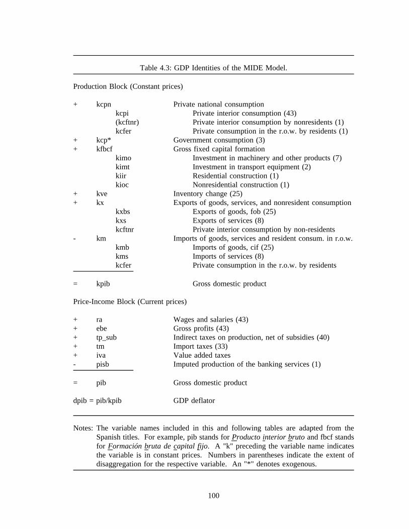
Table 4.3: GDP Identities of the MIDE Model.
Production Block (Constant prices)
+ kcpn Private national consumptionkcpi Private interior consumption (43)(kcftnr) Private interior consumption by nonresidents (1)kcfer Private consumption in the r.o.w. by residents (1)
+ kcp* Government consumption (3)+ kfbcf Gross fixed capital formation
kimo Investment in machinery and other products (7)kimt Investment in transport equipment (2)kiir Residential construction (1)kioc Nonresidential construction (1)
+ kve Inventory change (25)+ kx Exports of goods, services, and nonresident consumption
kxbs Exports of goods, fob (25)kxs Exports of services (8)kcftnr Private interior consumption by non-residents
- km Imports of goods, services and resident consum. in r.o.w.kmb Imports of goods, cif (25)kms Imports of services (8)kcfer Private consumption in the r.o.w. by residents
= kpib Gross domestic product
Price-Income Block (Current prices)
+ ra Wages and salaries (43)+ ebe Gross profits (43)+ tp_sub Indirect taxes on production, net of subsidies (40)+ tm Import taxes (33)+ iva Value added taxes- pisb Imputed production of the banking services (1)
= pib Gross domestic product
dpib = pib/kpib GDP deflator
Notes: The variable names included in this and following tables are adapted from theSpanish titles. For example, pib stands for Producto interior bruto and fbcf standsfor Formación bruta de capital fijo. A "k" preceding the variable name indicatesthe variable is in constant prices. Numbers in parentheses indicate the extent ofdisaggregation for the respective variable. An "*" denotes exogenous.
100

4.3 The Accountant
The role of the accountant is to determine the total disposable income of the nation
from the nominal GDP, and distribute this income to households, corporations and
government. The four major identities are displayed in Table 4.4. Several important
macroeconomic quantities must be modelled at this stage, other variables are assumed
exogenously. Table 4.5 identifies, and lists the influences on, each of the endogenous
variables.4
The first identity is for the determination of Net national disposable income from Gross
domestic product. To determine this quantity, we must model Capital consumption, deduct
it from GDP, and add several exogenous international income flows. The second identity
computes the Net household disposable income. This computation requires the modeling
of net interest and dividend income, the calculation of several taxes from exogenously
specified tax rates on gross income, and various exogenous transfer payments. The
household disposable income then feeds back into the product block as an input into the
determination of aggregate consumption. Household savings is then computed as the
difference between income and consumption. The last two identities shown in Table 4.4
are for the Government surplus (deficit) and the Balance on the current account. These
quantities are necessary for interest payments and interest rate equations. More importantly,
as we shall see below, the current account balance becomes an important variable for
judging the overall performance of the model.
4 The accounting identities, and much of the data used for them, come from the workof Corrales and Taguas (1989). Several ideas for modeling the quantities were borrowedfrom the MOISEES model constructed at the Ministerio de Economía y Hacienda asdescribed in Dirección General de Planificación (1990).
101

Table 4.4: Macroeconomic Identities of the Accountant.(current prices)
1) Net national disposable income
+ pib Gross domestic product- ccf Total fixed capital consumption
ccfe Corporate fixed capital consumptionccff Household fixed capital consumptionccfap Government fixed capital consumption
+ subntrm (a) Subsidies net of taxes received from the r.o.w.+ ranrm Net wages and salaries from the r.o.w.+ rpnrm (b) Net proprietor and corporate income from the r.o.w.+ trnrm (c) Other net current transfers from the r.o.w.
= rnnd Net national disposable income
2) Net household disposable income and savings
+ ebef Gross proprietor profits- ccff Household fixed capital consumption+ ras Wages and salaries+ ranrm Net wages and salaries from the r.o.w.- csf Social security taxes paid from wages and salaries+ rpnf Net interest and dividend received by households+ trnf (c) Net other current transfers received by households- tdf Direct taxes paid by households+ ps (c) Social security benefits paid by government+ ops (c) Other benefits paid by businesses
= rndf Household net disposable income/pcpn Consumption deflator
= krndf Real household net disposable income-kcpn Private national consumption in current prices
= ksnf Real net household savings
(a) - Variable completely exogenous to the model.(b) - Variable is exogenous to the model, but dependent on exchange rates, which are also
exogenous.(c) - Variable exogenous in real terms, but nominal quantity is dependent on an
appropriate endogenous deflator.
102

Table 4.4: Macroeconomic identities of the Accountant (continued).(current prices)
3) Government deficit
+ tp_sub Indirect taxes on production net of subsidies+ iva Value added taxes+ tm Import taxes+ csap Social security taxes received by the government+ td Direct taxes received by government
tdf Direct taxes paid by householdstde Direct taxes paid by corporations
+ intap Net interest received by government+ tynap (c) Net other transfers and income received by government- ps (c) Social security benefits paid by government+ cin (c) Current international cooperation+ subntrm (a) Subsidies net taxes received from the r.o.w.
= rndap Net disposable income of government
- cp (c) Government consumption- iap (c) Government investment+ ccfap Government fixed capital consumption- ant (a) Net asset purchases+ trkap (c) Net capital transfers to the government+ tk Taxes on capital
= confap Government surplus (deficit)
4) Balance of Payments - Current Account
+ x Exports of goods, services, and nonresident consumption- m Imports of goods, services, and resident cons. in the r.o.w.+ ranrm Net wages and salaries from the r.o.w.+ rpnrm (b) Net proprietor and corporate income from the r.o.w.+ trnrm (c) Net current transfers from the r.o.w.+ subntrm (a) Subsidies net of taxes received from the r.o.w.
= socrm Current account surplus (deficit)
+ trkrm (c) Net capital transfers from the r.o.w.
= confn Net financing surplus (deficit)
103

Table 4.5: Influences on Endogenous Macroeconomic Variables of the Accountant.
Variable Influences
Gross proprietor profits (ebef)
Gross government profits (ebeap)
Gross corporate profits (ebee)
Total fixed capital consumption (ccf)
Household fixed capital cons. (ccff)
Govt. fixed capital cons. (ccfap)
Corporate fixed capital cons. (ccfe)
Net wages & salaries from r.o.w. (ranrm)
Net interest & dividends received byhouseholds (rpnf)
Direct taxes paid by households (tdf)
Direct taxes paid by corporations (tde)
Direct taxes received by government (td)
Soc. sec. taxes rec. by the govt. (csap)
Pension contrib. rec. by corporations (cse)
Social security taxes & pension paymentsfrom wages and salaries (csf)
Total private sector gross profits (ebe)
Equal to sum of public sector gross profits
ebee = ebe - ebef - ebeap
Depreciation computed for invest. eqs.inflated by invest. price
Total fixed capital consumption
Equal to govt. gross profits (nationalaccount identity)
ccfe = ccf - ccff - ccfap
Unemployment rateExchange rate
Dist. lag on corporate after-tax net profitsDist. lag on real interest rateDummy variable for financial deregulation
Taxable household incomeUnemployment rate
Net corporate profits
td = tdf + tde
Total wages and salariesExogenous tax rate
Exogenous
csf = csap + cse
104

Table 4.5: Influences on Endogenous Macroeconomic Variables of the Accountant(cont.)
Variable Influences
Net interest paid by government (intap)
Taxes on capital (tk)
Long-term interest rate (rlp)
Accumulated govt. deficit times effectiveinterest rate at time of deficit
Distributed lag on interest rates
Current period nominal investment
M2 to nominal GDP ratio, current andone lagged period
Weighted average of current and pastinflation
Current account deficit as percentage ofnominal GDP
Dummy variable for deregulation ofcapital markets
Due to the absence of homogenous historical interest rate series, the present version of
MIDE contains only one interest rate variable. This variable is the long-term rate paid on
the government debt. It was extended back from 1978 using the information provided by
Baiges, et al. (1987). This rate is important in equations for consumption and income flows.
The explanatory variables used in the behavior equation which projects the interest rate are
shown in Table 4.5. The major influence in the equation is the level of the money supply
relative to the nominal GDP. The level of the current account deficit relative to the GDP
also has an important effect here.
It is useful to end this description of MIDE with a summary of the important
characteristics and properties of the model. Specifically, the MIDE model contains:
1) An aggregate consumption function which smoothes the effects of changes inincome. It also integrates a wealth effect designed to stifle demand during
105

periods of high inflation. Increases in unemployment also dampen demand.
2) Investment accelerator functions which respond to activity in the investingindustries and relative investment to production prices. The investmentfunctions also depend on monetary conditions. At a given money supply,periods of slack demand and low prices imply monetary ease and domesticdemand is stimulated. High demand and high prices will encourage theopposite effect.
3) Export equations which depend on demand conditions in Spain’s tradingpartner countries, relative prices and exchange rates. Similarly, the importfunctions depend on domestic demand and the relative price of imports todomestic production.
4) Sectoral potential output which is modeled with essentially exogenousproductivity trends. Excessive growth in demand will drive up prices throughlabor costs if the productivity level is not adequate. Rising prices choke offdemand.
5) A wage function which responds to recent inflation and the gap betweenunemployment and the "natural rate of unemployment".
6) Sectoral profit functions which respond to wage costs and, for tradeable goodsindustries, international prices and tariff rates. Therefore, domestic prices aresensitive to foreign competitive pressures.
Some of these points may not be completely clear after a first reading of this chapter.
However, they are explained in detail in the following chapters. For now, an example of
how these mechanisms work to stabilize the model is helpful.
Since Spain is an open economy with a substantial dependence on foreign trade, the
import and export equations play a key role for in the model. In the first place, increases
in domestic demand lead to higher prices by increasing wages and profit margins, resulting
in increased imports both because of relatively high income elasticities of demand and lower
relative import prices. This increased import penetration tends to moderate pressure on
domestic manufacturers. Domestic inflation also decreases exports, which works to stabilize
the demand and price increases. Decreasing domestic demand will have the opposite effect
106

of stifling imports and increasing exports, stabilizing the economy. Therefore, attempts to
stimulate or slow the economy through monetary or fiscal policies will have only limited
effects. Because this phenomenon is so important in the workings of the model, I have not
imposed an explicit balance of payments constraint on the model. On the other hand, the
balance of payments as a percentage of GDP is often the first quantity to be examined in
any given simulation of the model. If the model projects what appears to be an untenable
balance of payments, this is taken as a signal that exogenous assumptions, such as exchange
rates, money supply, and government consumption, or equation parameters need to be
revised.
4.4 Criteria for Equation Specification and Evaluation of Econometric Results
In A Guide to Econometrics, Peter Kennedy (1985) states that the skill of the
econometrician lies in the judicious combination of sensible economic theory as well as
sound statistical methods. In the words of Malinvaud:
The art of the econometrician consists in finding the set of assumptions which areboth sufficiently specific and sufficiently realistic to allow him to take the bestpossible advantage of the data available to him (1966, p.524).
Moreover, the economic theory behind functional forms and the statistical procedures used
to estimate these forms is influenced by the underlying rationale for performing the
econometrics in the first place. For the MIDE model, the ultimate role of each individual
behavioral equation is to provide an estimate of the dependent variable which will be used,
in conjunction with other similarly estimated variables, in a highly detailed economic model.
This special purpose gives rise to a methodology of equation specification and estimation
107
which diverges in a number of ways from more traditional research. This section first
provides a description of the criteria I used to formulate the equation specifications of the
MIDE model. It then lists some criteria that I used to evaluate the econometric results of
the equation estimations.
Five specific criteria guide the selection of functional forms. The first two
considerations are practical ones. First, the equations must include only variables that are
available from official sources or can be reasonably constructed from official data. Earlier
in this chapter, we encountered situations where the lack of quality data dictated the
structure of the MIDE model. We shall see further illustrations in following chapters.
Secondly, the functional forms of the equations should be relatively easy to estimate given
existing human and computer resources.
The third criterion is that the equations must contain properties which are consistent
with the actual behavior within commodity markets and account for the most important
influences on the dependent variable. Such factors may include distributed lags on
explanatory variables, or factors exogenous to the entire model. To satisfy this criterion,
it is neither necessary nor sufficient that a functional form used to predict economic
quantities be directly derived from neoclassical optimization theory. The consumption and
labor supply functions are not based on utility maximization of a "representative agent"; nor
are industry production functions derived from profit maximization of a "representative
firm."
This fact does not imply any contradiction with micro-maximizing behavior. Rather,
it recognizes that the empirical implementation of strict microeconomic theory on an
aggregate level can be unnecessarily restrictive. For example, in the case of consumption
demand, Slutsky symmetry (i.e. the equivalence of compensated cross-price elasticities)
108

generally does not aggregate over individuals with different incomes, different utility
functions, and through time. Therefore, aggregate consumption equations fully consistent
with microeconomic utility maximization need not satisfy Slutsky symmetry. In the case
of firms, only rather complex maximizing problems can give the sort of distributed lags
which we in fact observe at the aggregate level. The fact that the lag patterns used in the
model cannot be derived from oversimplified functions does not make them inconsistent
with maximizing behavior.
Also, data limitations sometimes require that behavior modeling be less grounded in
theory than we might desire. For example, conventional theory and econometric practice
often assign important roles to sectoral capital stocks for determination of investment,
international trade, productivity or profits. However, the absence of such data for Spain
restricts us to more ad hoc specifications that use other variables to detect the presence of
capacity constraints. Finally, as mentioned in the previous chapter, the solution to the
MIDE model is constructed under the assumption of relatively rigid markets in the short
run, with adjustment to full employment equilibrium in the longer run. Therefore, functions
derived from neo-classical general equilibrium theory may be inconsistent with the reality
of an economy in disequilibrium.
The general framework and stability of the model is a fourth consideration for choosing
explanatory variables for each equation. In forecasting, every explanatory variable must be
produced by the model or specified exogenously. Therefore, exogenous variables which
have a marginal effect on dependent variables are excluded if forecasting these variable
themselves is difficult. One example of this consideration is the omission of a variable for
sectoral unemployment for industry wage equations. While historic series for this variable
are available and would undoubtedly contribute to the estimation of wages, forecasting
109

sectoral unemployment into the future requires difficult assumptions about labor force
mobility. On the other hand, estimated equations may include coefficients which are
"insignificant" from a statistical point of view, but which are necessary to provide important
interactions, consistent from a theoretical point of view, and important in the context of the
overall model.
The fifth and final criterion is that the functional form must have desirable long-run
properties. The concern for the long-run properties of the equations has led to the almost
total exclusion of the use of the lagged dependent variable as an explanatory factor. The
use of this technique is often justified by reference to distributed lags or adaptive
expectations, or as an error correction device. The truth is that it works well because the
lagged dependent variable has, of course, the same trend as the dependent variable itself.
For long-term models, we are interested in explaining the trend, not temporary deviations
from the trend. An equation using the lagged dependent variable will not capture the
fundamental structural influences on the dependent variable and will predict poorly in the
long run. Without the lagged dependent variable, there is often substantial autocorrelation
of the residuals in the equation. More often than not, however, autocorrelation is because
important explanatory variables are omitted for lack of data. Recognizing that this is the
case, the autocorrelation coefficient is used as an error correction mechanism in making the
forecasts for the first few periods.
The error correction mechanism used for most of the equations of the MIDE model is
known as the "rho adjustment." In this technique, the predictions in the forecast period
given by the equation is adjusted by the error in the last year of the estimation period
multiplied by the autocorrelation coefficient raised to the power of the forecast period, i.e.:
110

y1’ = y1 + r0 × ρy2’ = y2 + r0 × ρ2
. . . .yn’ = yn + r0 × ρn
where yn’ is the model’s prediction in forecast period n, yn is the equation’s prediction, r0
is the error in the last period of the fit, and ρ is the autocorrelation coefficient. This error
correction mechanism is similar in spirit, but not equivalent in implementation, to the
cointegration error correction technique currently in vogue (see Engle and Granger 1987).
I made several attempts to use this mechanism in constructing the MIDE model, but
eventually abandoned the approach. The rho adjustment is considerably easier to implement
and has a much longer track record of successful use than the relatively new cointegration-
error correction technique. More important, it does not require that data used by the
equation possess the integration and cointegration properties needed to implement the
cointegration technique (I will have more to say about this in the following chapter). In my
experimentation with this new technique, I have found that it is often impossible to satisfy
the integration properties when working with disaggregated data. Furthermore, if one
simply assumes that the data satisfies the integration tests (as is common in the literature,
see, for example, Andres et. al 1990), the equation results are often so poor and are
unusable in a complete model. It was this final factor which persuaded me to stick with the
rho-adjustment.
In summary, the behavioral equation specifications of the MIDE model are intended to
satisfy five criteria: 1) they include variables for which data is easily obtainable, 2) they are
relatively easy to estimate, 3) they are consistent with actual economic behavior, 4) they are
consistent with the general framework underlying the entire model, and 5) they have
desirable long-run properties.
111
A second set of criteria must be established for evaluating and accepting estimation
results. In this work, we regard econometric techniques as simple tools used to construct
crude approximations of complicated processes, rather than complex statistical processes
used to prove or disprove simple hypotheses. The functional specifications are not regarded
as "true" equations, and there is no attempts to acquire "efficient" estimates of parameters.
The objective is to obtain parameters which depict plausible economic behavior, fit the
historic data reasonably well, and produce equation properties which work together to yield
a useful forecasting or policy analysis tool. Therefore, like the majority of those who have
constructed large disaggregated macroeconomic models, I chiefly employ ordinary least
squares or simple non-linear estimation techniques (see, for example, Barker and Peterson,
page 88).
Nevertheless, the importance of including independent variables in any given equation
can be judged using the traditional t-statistics. Preferable, however, is the "marginal
explanatory value," or "mexval." This statistic reports the percentage increase in the
standard error of the estimate if the independent variable was left out of the specification.
As a rule, the mexval is correlated with the t-statistic, but since it does not depend on any
underlying statistical assumptions, its use for evaluating the importance of independent
variable is more reliable. Another useful statistic is the elasticity of the dependent variable
with respect to the explanatory variable. This figure assists in judging the reasonableness
of the magnitude of the parameter estimate.
Other considerations for evaluating econometric results include the stability of the
parameters when estimated over different estimation periods, and the accuracy of out-of-
sample predictions given by the parameters. Parameter estimates that are not robust may
not be suitable for a five or ten year forecast. Moreover, drastic changes in parameter
112

values between two estimation periods often indicate the presence of structural or behavioral
change through time. Poor out-of-sample predictions can also signal structural change. The
model builder must be aware of such change when constructing and implementing the
model. In the building of MIDE, the examination of estimated equations with these criteria
has been very important since the structure and behavior of the Spanish economy has
changed significantly over the past four years.
Regression exercises often provide inappropriate parameter estimates for use in a long-
term forecasting model. When unsatisfactory estimates occur, it may be required to use
Bayesian techniques which combine apriori subjective knowledge about the economy with
the quantitative data to determine parameters which work well in the general model. To
attain more reasonable estimates I employ "soft constraints" on the parameter values.
Instead of minimizing the sum of squared residuals, a linear combination of the sum of
squared errors and the deviations from the constraint is minimized. Observations imposing
the constraint are added to the data and integrated into the least squares process. These
techniques are often called "stochastic constraints" or "Theil’s mixed estimation" or
"Bayesian regression." Soft constraints are used in two ways in the work: one forces a
single parameter to approach an apriori value, the other is the Almon procedure for the
estimation of polynomial distributed lags on the independent variables.5 When soft
constraints are used, the addition of observations makes the use of standard errors, t-
statistics and mexvals for parameter estimates questionable and difficult to interpret. They
are therefore not included in the displays of regression results when the technique has been
used.
The econometric approach outlined above sacrifices the theoretical benefits of
5 For a complete description of soft constraints, see Almon (1989), pages 107-116.
113
consistency and cross equation error information which can be obtained by using system
estimators, such a Full Information Maximum Likelihood. One reason for this is that is
often impractical to implement system estimation because of the computational expense
involved. For instance, it is often required to re-examine the specification and estimation
of a single equation which is producing bad results in the general model. System
estimation, however, would require the re-estimation of the entire system of equations in
these cases. Furthermore, sectoral level behavioral equations do not contain much of the
simultaneity which characterizes macroeconomic functions. For example, in a
macroeconomic model it may be unsatisfactory to regard output as an exogenous variable
in an aggregate investment equation since it contains the investment explained. In a
disaggregated model, however, the exogeneity assumption is appropriate, and the need for
the use of instrumental variable regression techniques is reduced.
A final constraint which often limits the application of the most sophisticated
econometric techniques is the quality of the data. Kennedy (1985) illustrates this point with
a quote from Valavanis:
Econometric theory is like an exquisitely balanced French recipe, spelling outprecisely with how many turns to mix the sauce, how many carats of spice to add,and for how many milliseconds to bake the mixture at exactly 474 degrees oftemperature. But when the statistical cook turns to raw material, he finds thathearts of cactus fruit are unavailable, so he substitutes chunks of cantaloupe; wherethe recipe calls for vermicelli he uses shredded wheat; and he substitutes greengarment dye for curry, ping-pong balls for turtle’s eggs, and, for Chalifougnacvintage 1883, a can of turpentine (1959, p.83).
Such problems are especially pervasive when working with disaggregated data. The Spanish
economy data used for the construction of the MIDE model are derived from several
different sources. Often, the sources use different collection methods and may use different
114

industry definitions for the data. Moreover, time series presented by the same source can
suffer ruptures in data definitions or coverage which makes the series heterogeneous across
time.6 In the following chapters, we will observe cases where the unfortunate quality or
quantity of sectoral level data precludes the estimation of equations with good econometric
properties. The application of more sophisticated techniques rarely, if ever, is a solution to
these problems. Moreover, to bundle the bad data with good data in a full system
estimation can compound the problems. Therefore, the reliance on simple, straightforward
methods is justified, especially where they yield sensible economic properties with little
computational expense.
A final, and most important consideration, underlies both the definitive selection of
functional form and the acceptance of estimation results for each equation of the MIDE
model: the simulation and forecasting performance of the equation once it is inserted into
the model. Often, equations which are reasonable both theoretically and econometrically
often combine in a model to produce an unstable model or unreasonable results. At this
stage, the model builder must return to the proverbial drawing board to re-specify and re-
estimate one equation, a whole set of equations or several sets of equations. This scenario
occurred several times during the construction of MIDE. Finally, however, the equations
specifications and parameter estimates fell into place to produce a solid simulation model.
The next three chapters describe these equations.
6 Details of sources and methods used for the compilation of the data base of the MIDEmodel are given in the Appendix.
115

CHAPTER 5:
EQUATION SPECIFICATION AND ESTIMATION:
CONSUMPTION AND FIXED INVESTMENT
5.1 Private Consumption
Private consumption expenditure constitutes the lion’s share of demand for every
economy. For the Spanish economy, it typically accounts for 60 to 70 percent of GDP.
Thus, the determination of private consumption is the crucial part of a macroeconomic
empirical model. For a disaggregated model, the commodity composition of private
consumption also becomes very important. The MIDE model takes a two step approach.
In the first step, it determines total Private national consumption as a function of income,
wealth, unemployment and interest rates. To attain Private interior consumption, MIDE
subtracts Exterior consumption by Spanish residents and adds Interior consumption by
nonresidents from the national consumption figure. In the second step, a system of
commodity demand equations allocates Private interior consumption among the 43 products
enumerated in the 1980-based, national accounts classification.
This section will cover each of these stages in turn. The first task is to provide the
specification and estimation for the aggregate consumption equation. (Chapter 6 covers
behavioral equations for Exterior consumption by residents and Interior consumption by
nonresidents.) The following pages describe the system and provide the results for the
disaggregated consumption equations.
116

Aggregate Private National Consumption
Over the years, various forms of aggregate consumption equations have been posited
and estimated. A simple Keynesian function, where consumption is dependent on disposable
income, inspired the original equation forms. Later, more elaborate functions integrated the
permanent income hypothesis of Friedman. These approaches use distributed lags of
changes in income as well as the current level. Recent approaches have attempted to
integrate wealth and/or inflation effects into the consumption function (see, for example,
Holtham and Kato 1986). This approach was influenced by the observation that high
inflation in the 1970’s tended to decrease the proportion of consumption to disposable
income. There are several reasons that this may be so, but the most convincing is that
inflation tends to devalue the stock of wealth and people increase savings in order to
maintain their asset stock. Specifications intended to capture this effect have varied. Some
have attempted to include variables for real wealth, others have included the inflation rate,
while still others have included both variables.
Recent research on consumption in the Spanish economy, conducted for construction
of the MOISEES model, is Andres et al. (1990 - henceforth Andres). Their functional form
uses the cointegration error correction methodology pioneered by Engle and Granger (1987).
In this type of equation estimation, the specification distinguishes between explanatory
variables that have a permanent effect on the dependent variable and those which have a
transient effect on the dependent variable. An explanatory variable is determined to have
long-term equilibrium relationship if it is "cointegrated" with the dependent variable.
Variables are cointegrated if 1) each is integrated with degree of one (i.e., their first
difference is stationary) and 2) a linear combination of the variables (e.g., a regression
equation) produces a stationary series. Andres, after a rather tortured sequence of
117

increasingly complicated Dickey-Fuller tests, shows that the hypothesis of cointegration for
Spanish series of aggregate consumption, disposable income and wealth cannot be rejected.
(Wealth is the broad money supply (M4) plus the real stock of bonds held by consumers,
deflated by the consumption deflator, plus the stock of real private capital.)
The consumption equation of the MOISEES model, therefore, postulates a long term
relationship between consumption and disposable income and wealth. The final functional
form is estimated for the first difference in the log of consumption. Andres integrates the
long-term income-wealth relationship into the final functional form by including, as a right
hand side variable, the lagged residuals of the double-log OLS equation of consumption on
current income and wealth (the cointegration equation). This variable is called the error
correction term.
The functional form, which does not include an intercept, also includes the lagged
dependent variable and several "short run" variables. First, the change in the log of real
disposable income enters the equation with a positive coefficient that is less than the
long-run marginal propensity to consume. This magnitude of the coefficient reflects that
increases in income do not translate immediately into an equal increase in consumption, but
are partly absorbed by savings (the permanent income effect). The equation also includes
the second difference in the log of real wealth and the second difference in the log of the
inflation rate. The coefficient on the second variable is negative, suggesting, as reasoned
above, that consumers increase their savings rate with higher inflation. It is not clear,
however, why all three influences (real income, real wealth and inflation) are present in this
equation. The consumption deflator already enters in the equation in the computation of real
income and real wealth. The authors explain that it can be considered a further short-run
"inflation tax" on income and wealth (Andres et al. 1990, pp. 8-9). Finally, the last
118

variables in the equation, the second difference in the unemployment rate and the first
difference of the real interest rate, display negative signs on the coefficients.
Based on sophisticated econometric theory, and currently quite fashionable, the
cointegration approach is attractive. However, in the interest of simplicity, I have not
adopted the approach here. For example, in the Andres paper, over 25 pages of regressions
and statistical tests conclude that the hypothesis of cointegration among consumption,
income and wealth cannot be rejected. Notably, it is difficult to show that the first
difference of the consumption and income series are stationary, without segmenting the
series into different periods. In other words, they accept their a-priori hypothesis that
consumption depends on income and wealth because there is no statistical evidence to refute
it. The current work, however, does not have the space to devote to an exercise that does
not reject to a hypothesis that is not only an accepted pillar of economic theory, but self-
evident. Moreover, I find the final equation of Andres very difficult to interpret. The
inclusion of the error-correction term makes the derivation of the income and wealth
elasticity on consumption a formidable task. I prefer a simpler equation that is easier to
interpret. Autocorrelation problems can be avoided by differencing of variables, and error
correction for forecasting can be handled by the simple rho adjustment described in the
previous chapter.
The consumption function for the MIDE model conserves most of the influences of the
MOISEES aggregate consumption equation. The functional form is:
∆ lnCPCt a∆ lnYPCt b∆lnYPCt 1 c∆lnWPCt d∆lnUt e∆lnRt 1
where: CPCt = real private national consumption per capita in year t,
YPCt = real household disposable income per capita,
119

WPCt = real private wealth per capita,
Ut = the unemployment rate, and
Rt = the nominal interest rate.
The equation is estimated in per capita terms to factor out the increases in consumption
which occur from population growth from those which result from increases in the other
variables. Wealth is defined as the broad money supply (M4) deflated by the national
consumption deflator, plus the real housing stock at beginning of the year times the relative
price of residential construction to aggregate consumption. One advantage of using this
definition of wealth in the consumption equation is that the money supply has a positive
impact on aggregate demand in the model. This wealth definition differs from the Andres
equation because it uses a narrower definition of capital stock and excludes bonds held by
consumers. While the bonds are undoubtedly an important component of wealth, there is
not much hope in projecting this quantity without a full blown financial submodel. The
housing stock is multiplied by the relative price of residential construction in order to
revalue the stock at current market prices. The equation also contains a dummy variable for
1976, also used by Andres, which accounts for a steep fall in consumption which cannot be
explained by the included variables. Table 5.1 displays the estimation results.
The first equation of Table 5.1, estimated from 1967 through 1990, is the result
included in the MIDE model. Since subsequent regression results will be presented with
similar tables throughout this paper, a brief explanation of some of the terms is in order:1
SEE = Standard error of estimate (i.e., the square root of the average of thesquared residuals).
1 The table is adapted from results given by the G data base and regression programcreated by Almon (1989).
120

SEE+1 = SEE for forecasts one period ahead using the rho adjustment.
MAPE = Mean absolute percentage error.
RSQ = R-squared, or the coefficient of multiple determination.
RBSQ = R-bar-squared, the R-squared adjusted for degrees of freedom.
RHO = Autocorrelation coefficient of the residuals.
DW = Durbin-Watson statistic.
Obser = Number of observations.
DoFree = Degrees of freedom.
Mexval = Marginal explanatory value: percent change in SEE if the variablewas left out of the equation.
T-stat = Student t values.
Each coefficient has the expected sign and is of reasonable magnitude. One interesting
result is that the lagged difference in the nominal interest rate performs better than the
contemporary change under a variety of specifications and estimation periods. In contrast
to Andres, however, the real interest rate could not enhance the fit of the equation and often
displayed the wrong sign. Figure 5.1 illustrates the fit for the model’s equation. Especially
in the later years, the parameters capture the turning points of the differenced series quite
well. From this graph, we can also note why Andres had such a difficult time in proving
that the consumption series is stationary. Over this interval, the first difference of
consumption certainly displays different means for the three different periods of the economy
discussed in Chapter 2. Most of the other macro magnitudes of the Spanish economy
display similar behavior.
The second equation displayed in Table 5.1 shows the same equation estimated from
1967 through 1986, with the out-of-sample predictive power tested through 1990. The
121

standard error of the estimate and mean absolute value for the test period confirm that the
equation predicts well. The specification is also robust. Parameter estimates for the income
and wealth terms are similar in magnitude to the first equation. However, the coefficients
Table 5.1: Estimation Results for Private National Consumption
Equation 1: 1967 - 1990, no inflation termSEE = 0.00706 RSQ = 0.9231 RHO = 0.35SEE+1 = 0.00670 RBSQ = 0.9018 DW = 1.31MAPE = 79.89 Obser = 24 DoFree = 18
Variable Reg-Coef Mexval t-value Mean0 dlcpc - - - - - - - - - - - - - - 0.02751 dlypc 0.43507 45.2 4.466 0.02432 dlypc(t-1) 0.21651 15.2 2.429 0.02463 dlwpc 0.25349 37.7 4.015 0.05294 dlunrat -0.02815 10.6 -2.009 0.10915 dlr(t-1) -0.05732 22.3 -2.986 0.02126 dum76 0.02659 23.4 3.065 0.0417
Equation 2: 1967-1986, no inflation term,ex-post forecast to 1990.
SEE = 0.00650 RSQ = 0.9379 RHO = 0.25SEE+1 = 0.00643 RBSQ = 0.9157 DW = 1.50MAPE = 85.25 Obser = 20 DoFree = 15Test (1987-90): SEE = 0.01126 MAPE = 19.12
Variable Reg-Coef Mexval t-value Mean0 dlcpc - - - - - - - - - - - - - - 0.02371 dlypc 0.44953 33.0 3.280 0.02082 dlypc(t-1) 0.19237 15.5 2.159 0.02233 dlwpc 0.21729 24.8 2.794 0.05404 dlunrat -0.01647 4.6 -1.148 0.14485 dlr(t-1) -0.04251 6.3 -1.345 0.02386 dum76 0.02520 28.6 3.027 0.0500
Equation 3: 1967-1990, with inflation termSEE = 0.00641 RSQ = 0.9367 RHO = 0.10SEE+1 = 0.00638 RBSQ = 0.9143 DW = 1.81MAPE = 87.44 Obser = 24 DoFree = 17
Variable Reg-Coef Mexval t-value Mean0 dlcpc - - - - - - - - - - - - - - 0.02751 dlypc 0.45734 56.9 4.986 0.02432 dlypc(t-1) 0.32093 26.8 3.221 0.02463 dlwpc 0.18206 18.3 2.606 0.05294 dlinfl -0.01396 10.2 -1.906 -0.00505 dlunrat -0.02026 6.2 -1.476 0.10916 dlr(t-1) -0.05298 22.7 -2.931 0.02127 dum76 0.02885 31.5 3.523 0.0417
122

Figure 5.1: Real Private National Consumption Equation, 1967-90.Actual vs. Predicted Values (change in logarithms).
on the unemployment and interest rate variables are significantly less powerful for this
period. For the interest rate, this could be expected. Recent interest rate and retail banking
deregulation have made consumer loans much more accessible and, therefore, consumption
more sensitive to interest rates. The mean absolute percentage error (MAPE) for the test
period also confirms that the equation is able to forecast this period.
Table 5.1 displays a third equation. The form of this equation includes the changes in
the log of inflation, as in Andres. It’s coefficient exhibits the correct sign. However, it does
not add to the explanatory value of the equation. The major effect of including the inflation
term is a decrease in the explanatory value of both unemployment and the interest rate. This
is undoubtedly attributable to multicollinearity among inflation, unemployment and the
nominal interest rate. Since, inflation already influences consumption through the real
income, real wealth and nominal interest rates terms I do not incorporate it in the final
model equation.
123

An Equation System for Consumption by Commodity Categories 2
In order to compute the commodity composition of aggregate consumption, MIDE
employs a system of estimated consumption equations. As with aggregate consumption, the
specification and estimation of such econometric consumption "systems" is an area of
abundant research activity.3 A system utilized in a forecasting model should exhibit several
features which reflect the behavior of real-world commodity markets and confer reasonable
long-term properties. Specifically, the functional form used for the present model is
designed to meet the following criteria:
1. It is capable of expressing either substitution or complementarity betweengoods. Moreover, it permits goods with close substitutes to have highprice elasticities and goods with no substitutes to have low priceelasticities.
2. It is homogeneous of degree zero in income and prices.
3. The sum of consumption of all the goods is equal to total consumption.
4. Price elasticities are independent of the level of income. Therefore, theconsumption equations cannot be additive functions of prices and income,for this implies that as income increases, price elasticities would decrease,an implausible result.
5. As income rises, the budget shares of individual commodities mustconverge to values between zero and one (i.e., the system should bestable).
6. The marginal propensities to consume out of income is different fordifferent goods. Furthermore, these propensities, and the asymptoticvalues of the budget shares should be allowed to depend on prices.
2 The functional form used for the MIDE consumption system is an adaptation of anonlinear functional form developed by Almon (1979). The following discussion of theproperties of consumption functions in general, and the Almon system in particular, borrowsheavily from that work.
3 For general surveys of this literature see Guayacq (1985), Brown and Deaton (1972)and Barten (1977). Lorenzo (1987 and 1988) offers another survey which estimates threepopular systems for the Spanish economy using four categories of goods.
124

Finally, the magnitude of the price dependence should be able to beestimated, not imposed by the functional form.
7. Non-price and non-income variables can be easily included in thefunction, and, as with income, the impacts of these variables should bedependent on prices. Moreover, price changes should alter the effects ofincome and non-income determinants in approximately equal proportions.
8. The number of parameters in the system is not so vast that they cannotbe estimated given the number of observations, and, furthermore, theparameters are relatively easy to estimate. Although aggregate marketdemand need not satisfy Slutsky symmetry, assuming that it holds in thebase year allows one to reduce the amount of parameters to estimate.
To attain these properties, the parameters for each of the consumption equations must
be estimated together in an integrated system of nonlinear functions. Almon (1979)
introduced the following system:
CPIi,t [ai biTt ci (Yt /Pt) di ∆(Yt /Pt) ] ×k
Pei,k
k,t
where: CPIi,t = the constant-price, per capita consumption expenditures forcommodity i in time t,
Tt = a time trend term or other relevant variables,
Yt = the total, per capita nominal private consumption,
pk,t = the nominal price index for commodity k, and
Pt = , where sk,o equals the budget shares in the basek
pk,t sk,o
year, where all prices are equal to one.
Essentially, the function is a linear term in total expenditure and other variables,
multiplied by a product of prices raised to various powers. The ai, bi, ci, di and ei,k’s are the
parameters for each equation. The specification of separate own and cross price elasticities
(ei,k) for each of the commodities fulfills requirement 1. While it will be necessary to reduce
125

the number of these parameters in the actual estimation, the desired properties will be pre-
served. The following restrictions are imposed on the parameters:
to give homogeneity of degree zero in total expenditure and prices,n
k 1
ei,k 0
i.e., requirement 2, and
to give constant-price adding-up, at constant relative prices.n
i 1
ci 1
The individual marginal propensities to consume out of total expenditure
( ) depend on prices (a point we shall come back to in a moment). This impliesδCPIi /δ(Y/P)
that, if relative prices change, the second of the above restrictions cannot (and surely will
not) guarantee that the individual quantities add up to aggregate consumption. To overcome
this violation of property 3, the MIDE model allocates the difference between total
expenditure and the sum of individual predictions across the consumption categories by the
use of a "spreader" term. Since the ci’s represent the marginal propensities to consume out
of total expenditure in the base year, and sum to one as required by the scaling procedure,
they are the spreader weights. It will be shown below that the amount allocated is quite
small.
The strength of this functional form is the multiplicative relation between the linear
term of the equation and prices. This type of form is superior to both linear and double log
(constant elasticity) forms. First of all, the form imposes a constant price elasticity
regardless of the level of total expenditure. For example, if the own-price elasticity is -1.0,
then a 5 percent increase in the relative price of a commodity leads to a 5 percent decrease
in consumption at any level total expenditure. This property satisfies requirement 4. A
126

system linear in price results in a falling price elasticity as demand increases over time, an
implausible property that is especially undesirable for long term economic modeling.
On the other hand, a strictly logarithmic function imposes constant elasticities on both
price and demand. In this case, if the income elasticity was greater than one, then
expenditures for individual goods would eventually exceed total income. In this
specification, as in a strictly linear function, the marginal propensity to consume the good
out of total expenditure remains constant for any level of expenditure. As long as that
quantity is below one, and practice has shown that the expenditure elasticity must be quite
high before it exceeds one, we can be assured the system is stable, fulfilling requirement 5.
On the other hand, the nonlinear formulation makes the marginal propensities to consume,
and therefore, the budget shares, depend on relative prices in a way that can be estimated,
providing the final properties under requirement 6.
It is precisely under these criteria (5 and 6) that other, more popular, equation systems
flounder. One example is "Almost Ideal Demand System" (AIDS) system of Deaton and
Muellbauer (1980). The estimation of this system invariably boils down to a double log
function of the budget share on relative prices and income. Since the elasticity of the budget
share with respect to income will be constant in such a system, it is probable that predicted
budget shares could exceed one (or fall to less than zero, since some of the coefficients must
be negative). This would be a particularly treacherous feature for multisectoral modeling.
Another popular formulation is the Rotterdam system of Barten (1967) and Theil (1967),
which is used in the estimation of the HERMES models (Dones et al. 1990). This system
assures adding-up for each year regardless of relative price changes. However, it
accomplishes the adding-up by imposing, through the functional form, a value for the price
elasticity of the marginal propensity to consume out of expenditure. For a description of this
127

point see Almon (1979). The Almon form, in contrast, sacrifices adding up to allow the
estimation procedure to choose the price elasticity of the marginal propensity to consume
out of income, rather than solving for it by hypothesis.
The linear term of the Almon equation can easily accept other explanatory variables.
Besides per capita total interior consumption, the MIDE model form includes a constant, a
time trend, and the first difference in total consumption as independent variables. The time
variable accounts for changes in trends, such as in tastes or the age composition of the
population, which cannot easily be modeled without additional data. The change in
aggregate expenditure term represents the change in total income, included to account for
incomplete consumption adjustments to income level. The coefficient on this variable could
have either sign, depending on the nature of the product. For most commodities it would
be expected to be negative. If income, and therefore total consumption, rises sharply, the
expenditure term predicts an immediate adjustment in demand for each good to the new
income level. However, in the first period, at least, a portion of the income increase would
be perceived by consumers as transitory. Therefore, a negative sign on the change in
consumption partially offsets the increase in predicted consumption due to the increased
level of income, reflecting consumption smoothing behavior. For other commodities, such
as consumer durables, the coefficient is positive to reflect a splurging effect when income
increases sharply. As with the total expenditure term, the influence of these variables is
affected by relative prices in identical proportions. This is requirement 7.
The form calls for an enormous number of parameters which easily exceed the number
of observations. To reduce the present theoretical system to one that can be estimated, two
modifications are made. The first is to impose symmetry in the base year, reducing the price
parameters by half. Slutsky symmetry states that the income-compensated, cross-price
128

elasticities for any two products are equal. In the base year, the compensated cross-price
derivative is:
(δqi / δpj)o
compensated = ei,j qoi / po
j .
Symmetry implies that:
ei,j (qoi / po
j) = ej,i (qoj / po
i) .
Rearranging the terms:
ei,j / ej,i = qoj po
j / qoi po
i = soj / so
i and, therefore,
ei,j / soj = ej,i /so
i ,
where the soi’s are budget shares in the base year. Now, if σi,j = ei,j / so
j, then σi,j = σj,i. The
σi,js become the parameters of the equations so symmetry can be easily imposed.
A second way to reduce the number of parameters to be estimated is by segregating
groups and subgroups of related commodities and impose the restrictions that the σ’s be
equal between all goods within the same group or subgroup. Furthermore, the σ’s between
goods not in the same group will also be equal, but different from the group σ’s. The
division of commodities into specific groups and subgroups is based on common-sense
knowledge of the relations between various commodities. Assumptions of complementarity
and substitutability between goods play a role in the selections. Table 5.3 shows the
grouping selected. For example, Expenditures for private use of vehicles and Vehicle
purchases, which are presumed to be complements, reside in the same "Private
transportation" subgroup. Therefore, there is a unique subgroup σ, which expresses the price
relationship between these two commodities. They are also in the "Transportation" group.
This grouping implies that Expenditures for private use of vehicles and Vehicle purchases
129

are assigned the same group σ, and are therefore are equally substitutable with,
Transportation services, the only other product in the group. Finally, all three commodities
are equally, and relatively weakly, substitutable with all unrelated goods within other groups.
This becomes clearer by examining the form of the estimated equation for a commodity in
group G (composed of subgroups A and B) and subgroup A:4
CPIi,t [ai bi Tt ci Yt /Pt di ∆Yt /Pt] × (pi,t /pA,t )σA × (pi,t /pG,t )
σG × (pi /Pt )σO
w h e r e :
pA (j∈ A
pj s oj )
1sA , sA
j∈ As o
j
pG (j∈ G
pj s oj )
1sG , sG
j∈ Gs o
j
σA sA (σA σG)
σG sG (σG σO)
For a product belonging to subgroup B, the A’s would be replaced by B’s. For products
which belong only to a group, and not an additional subgroup, the first price term referring
to subgroup A is not included. It is the group and the subgroup σ’s, and the individual ai’s,
bi’s, ci’s and di’s which are estimated. σo is the same for each product; σ’G is the same for
each product in group G; σ’A is the same for each product in subgroup A. If a σ’ is
positive, then the goods it relates are substitutes; if negative, complements.
The price of a product influences the demand for another product through its impact on
the relevant price indices, and that this impact is proportional to its budget share. For
instance, if product i and j are in the same subgroup, a change in the price of j influences
4 For a complete description of the simplification, see Almon (1979), pages 107-116.
130

Table 5.2: Income-Compensated Price Elasticity Formulaefor the Almon Consumption System
ηij = elasticity of demand for good i with respect to price j
For i in subgroup A and in group G:
ηii = -σ’A (1 - so
i / sA ) - σ’G (1 - so
i / sG ) - σo (1 - soi )
ηij = σ’A (so
j / sA ) + σ’G (so
j / sG ) + σo soj for j ∈ A, j ≠ i
ηij = σ’G (so
j / sG ) + σo soj for j ∈ G, j ∉ A
ηij = σo soj for j ∉ G
For i in group G, but not in any subgroup:
ηii = -σ’G (1 - so
i / sG ) - σo (1 - soi )
ηij = σ’G (so
j / sG ) + σo soj for j ∈ G, j ≠ i
ηij = σo soj for j ∉ G
demand for i through all three price terms pA, pG, and P, and therefore through each of the
three σ’s. The strength of the different effects are proportional to the budget shares of j in
each of the price indices. Additionally, if product k was also in this subgroup, a change in
the price of j would affect demand of k by the same percentage that it affects demand for
i. If j was in a different group than i, a change in the price of j would alter demand of i
only through P and the parameter σo. Moreover, this cross-price effect, which is
proportional to the budget share of j in P, is equivalent for all goods which are not in j’s
group. Therefore, quantifying the actual own and cross-price elasticities from the estimated
σ’s requires specific transformations of these parameters. A careful examination of these
transformations, displayed in Table 5.2, should clarify the above discussion.
131
Estimation of the System for Spain
The dependent variable for the regressions is per capita interior consumption of each
of the 43 commodity categories in 1980 prices, for the years 1964 through 1989. Since
disaggregated consumption data for 1964 through 1979 is published for private national
consumption, and then for only 31 products, the actual data used here was constructed as
described in Sanz (1989) and in the Appendix. While the commodity definitions were the
same for the years 1980 through 1989, the data was homogenized to the 1980 based national
accounts. Data was available in current and constant prices; price indices were constructed
from the ratio of the two. Current price total expenditure is the sum of the commodity
consumption. It is divided by population and deflated using the general interior consumption
price index to yield per capita constant-price total Private interior consumption.
For most of the commodities, expenditure elasticities estimates come from the
regression of cross-section data from the 1980-81 Household Budget Survey (Encuesta de
Presupuestos Familiares), published by the Instituto Nacional de Estadística (1983). This
survey of consumption provides data by commodity and income class. The elasticity is
estimated by regressing the logarithm of per capita consumption of each commodity on the
logarithm of total per capita consumption for each decile of income level. The independent
variable is total per capita consumption for it better reflects permanent income for a
particular year. For the detailed food categories, the Encuesta did not contain decile level
of consumption. Expenditure elasticity estimates for these goods were taken from Moltó,
et al. (1989). This work estimated elasticities using individual household observations from
the survey which produced the Encuesta. To be consistent with the adding up constraint,
the total expenditure elasticity estimates were scaled so their weighted average, using the
base year budget shares, is equal to one in that year (1980). They were then converted to
132

linear coefficients at the expenditure levels of the last year of the data. These coefficients
become the ci’s in the time series equation.
One influence on consumption not accounted for in the functional form outlined above
is the influence of financial conditions. While for most goods interest rates probably have
little influence, for some, such as expenditures on motor vehicles, it is important. Interest
rates are easily inserted in the linear term of the equation. However, because there is a high
degree of collinearity between the two variables, it is preferable to replace the time trend
with the interest rate variable. Initially, the interest rate was included in all the equations
for durable goods. However, Motor vehicles is the only commodity for which the
coefficient was both significant and displayed the proper sign. In the results presented
below, only this equation includes the interest rate.
In two other cases, dummy variables replace the time trend. The first case of this
occurs with Alcoholic beverages (Commodity 12). This dummy assumes the value of 0.0
from 1964 through 1974 and 1.0 for the rest of the years. It accounts for problems with the
data. In the second case, retail financial market reforms have evidently decreased,
dramatically, expenditure for Financial services (41). The equation requires a dummy to
capture this effect. To represent the progressionary nature of these reforms the dummy is
.5 for 1981, .75 in 1982 and 1.0 for each subsequent year.
To perform the estimation, a σo was chosen and used for all the groups. Each group
of equations was estimated concurrently in order to impose the equality constraints for the
group σ’s. The nonlinear estimation is done iteratively using the Taylor series linearization
of the demand function. The initial expansion values for the coefficients are the ordinary
least squares estimates computed when the group σ’s equal zero. In each case, three or four
iterations were required before the sum of squared errors fell by less than one percent. Then
133

another σo was selected and the process repeated.
The different values of σo attempted were .09, .1, .3, .5 and .7. The final choice of σo
depended on a combination of evaluating the reasonableness of the parameters and the fit
of the equations. The value of .3 was chosen under this criterion. Several of the group
price elasticities are the result of softly constraining the σ parameters to take on feasible
values while trading off some of the fit. In the Household expenditure group, for example,
unconstrained regression produced positive own price elasticities for four of the five
commodities, and the group elasticities displayed strong complementarity. In addition to
conflicting with a-priori views for these parameters, the inclusion of such values in a larger
model could make that model unstable. Therefore, the group σ was softly constrained to
the value of .3. This was sufficient to produce reasonable parameters. The results for all
the commodities are presented in Table 5.3.
Each row of the table displays the commodity number, subgroup number and title for
each of the goods. We find subgroups only in the food, household operation, and transport
groups. The first column after the title is the total expenditure elasticity. The second
column displays the coefficient on time (or the dummy where applicable) as a percent of the
actual per capita consumption in the last period, except for Motor vehicles where it displays
the elasticity of per capita expenditure with respect to interest rates, evaluated at the mean
values of the variables. The next four columns contain price elasticities. The first contains
the own price elasticities, which are always negative. The second price parameter is the
group elasticity, which indicates the percentage effect on the demand for other products in
the same group, but not the same subgroup if this is relevant, if the price of that product
134

Table 5.3: Summary of Commodity Consumption Equations
No. SG Type of Good Expend. Time in % Price elasticities mape rsq rhoElast. last yr. Own Group Subgrp Genrl
Group 1: Food, Beverages and Tobacco1 10 Bread and cereals 0.17 0.1 -.269 -.002 .024 .009 1.7 .46 .322 9 Meat 0.59 -0.1 -.241 -.006 .039 .022 4.5 .88 .793 9 Fish 0.78 0.2 -.265 -.002 .015 .009 3.0 .67 .414 9 Milk, cheese & eggs 0.47 -0.1 -.260 -.003 .020 .011 2.8 .95 .695 10 Oils and fats 0.78 -0.4 -.282 -.001 .011 .004 2.6 .34 .646 10 Fruits & vegetables 0.78 0.2 -.258 -.003 .035 .013 3.3 .47 .757 10 Potatoes & oth. tubers 0.78 0.1 -.288 .000 .005 .002 6.3 .27 .728 10 Sugar 0.16 -0.4 -.291 .000 .002 .001 3.5 .79 .749 10 Coffee, tea & cocoa 0.39 -0.6 -.287 -.001 .006 .002 6.1 .49 .7410 Oth. food products 1.25 0.1 -.287 -.001 .006 .002 4.6 .81 .8511 Non-alcoholic bever. 0.78 0.3 -.270 .000 .025 .001 5.6 .56 .7612 11 Alcoholic beverages 0.78 -0.4(a) -.222 -.001 .073 .004 5.7 .34 .8513 Tobacco products 0.78 -0.3 -.197 -.001 .003 3.8 .94 .76
(a) Statistic is for dummy coefficient = 1 for 1975-89, 0 otherwise.
Group 2: Personal goods and services14 Clothing 1.57 0.0 -.211 -.075 .018 1.6 .95 .3515 Shoes 1.25 -0.3 -.159 -.024 .006 5.3 .73 .7737 Personal care prod. 0.78 -0.2 -.152 -.017 .004 3.1 .98 .5438 Oth. articles n.e.c. 1.25 -0.4 -.153 -.017 .004 3.9 .95 .55
Group 3: Household expenditures16 12 Rents & water 0.63 -0.6 -.178 -.124 -.200 .042 2.7 .98 .5017 12 Heat & light 0.63 -0.1 -.011 -.021 -.034 .007 4.2 .97 .8422 13 Maint. goods & serv. 0.63 0.3 -.341 -.013 .344 .004 7.0 .73 .9123 13 Domestic services 1.57 0.0 -.432 -.009 .253 .003 4.1 .74 .6932 Communications 1.57 0.1 -.074 -.007 .003 15.4 .90 .93
Group 4: Household durable goods18 Furniture 1.88 -0.6 -.701 .165 .007 5.5 .70 .8219 Household textiles 1.17 0.7 -.786 .080 .003 2.4 .92 .4020 Domestic appliances 1.72 1.0 -.770 .095 .004 5.4 .82 .5921 Domestic utensils 1.57 -0.3 -.812 .054 .002 3.8 .88 .6233 Entertainment goods 1.88 0.3 -.671 .195 .008 2.6 .97 .25

Table 5.3: Summary of Commodity Consumption Equations (cont.)
No. SG Type of Good Expend. Time in % Price elasticities mape rsq rhoElast. last yr. Own Group Subgrp Genrl
Group 5: Health and Medical Expenditures24 Drugs 1.25 0.1 -.410 .102 .005 11.7 .64 .9125 Therapeutic apparatus 1.46 -0.7 -.501 .012 .001 7.3 .76 .7226 Prof. medical serv. 1.64 0.0 -.451 .062 .003 4.3 .95 .6427 Hospital services 2.30 -0.5 -.481 .031 .002 5.3 .91 .7528 Priv. medic. insurance 1.73 -0.1 -.495 .017 .001 3.6 .94 .64
Group 6: Transportation29 14 Motor vehicles 1.57 -.245(b) -.272 .034 -.006 .009 11.0 .92 .7130 14 Vehicle expenses 1.00 0.0 -.279 .080 -.013 .022 3.7 .99 .8231 Transport services 1.58 0.1 -.376 .023 .006 5.5 .91 .87
(b) Statistic is interest elasticity at average expenditure and interest rate.
Group 7: Educational goods35 Books & periodicals 1.78 -0.8 -.221 -.027 .002 3.1 .92 .3636 Education 1.57 -0.1 -.266 -.071 .006 3.4 .84 .82
Group 8: Other Services34 Entertainment serv. 1.88 -0.4 -.547 .034 .005 3.4 .92 .7039 Restaurants & hotels 0.63 0.3 -.337 .244 .034 4.7 .95 .8340 Travel services 0.63 0.2 -.577 .004 .001 13.3 .71 .9241 Financial services 2.82 -2.0(c) -.561 .020 .003 6.7 .93 .3242 Other services 0.78 -0.2 -.576 .006 .001 7.4 .95 .8043 Oth. expend., n.e.c. 2.25 -0.4 -.563 .019 .003 19.3 .71 .92
(c) Statistic is for dummy coefficient = .5 for 1981, .75 for 82, 1 for 83-89, 0 otherwise.

increases by one percent. The subgroup elasticity shows the same cross-price effect within
a good’s subgroup. Finally, the general price elasticities show the impact of a price increase
for the product on the demand for all products outside the product’s group. A positive value
for a cross price elasticity signifies that the products which it relates are substitutes, a
negative value indicates complements. The last three columns exhibit the mean absolute
percentage errors, the R-squares and rhos (autocorrelation coefficients) for each equation.
In general, the parameters exhibit reasonable values and the fits of the equations are
satisfactory. Low values for the time trend parameter suggest that the income and price
variables provide most of the explanatory power in the equations. The magnitudes of the
own price elasticities are sensible. Necessities, such as food, rent, heat and light, and those
with no close substitutes, such as education and clothing, have relatively low own-price
elasticities. Durable goods, luxuries and items with close substitutes have higher own-price
elasticities. An exception is the purchase of Motor vehicles (Commodity 29) which has a
relatively low own-price elasticity.
The values for cross-price elasticities are small. Within most of the groups and
subgroups, the products are substitutes. The exceptions are the Food and Education groups
and the Private transportation subgroup. This result in the food group indicates that Meat,
Fish and Milk products (Commodities 2-4) are substitutes for each other, but complements
with all the other food categories. The same is true with all other foods and beverages. The
general cross-price elasticities suggest weak substitutability between products not contained
in the same group.
Many of the low R-squares for particular sectors result from data limitations rather than
problems with the method. For example, the series for Potatoes and other tubers
(Commodity 7) was separated from Fruits and vegetables (6) for the period previous to
137

1980. Apparently, these two series behaved quite differently during the income boom of the
60’s and early 70’s, but there is not enough information to capture these characteristics in
the regressions. While the Potatoes series would fit better with a much larger income
elasticity, it would not be realistic.
Figure 5.2 exhibits equations plots for some of the more important products. The ’s
represent the actual values and the +’s represent equation-predicted consumption. The
figures are for billions of pesetas in 1980 prices. The first plot displays the sum of all the
predicted values versus the actual total interior consumption. The striking behavior exhibited
by the actual series is one of very high growth through the early 1970’s, progressively
moderating growth through the late 70’s, almost no growth through 1984, and finally a
resumption of growth in 1985. The higher growth continued through 1989. Most of the
individual series, especially those for durable goods, display this behavior. It is clear that
the estimated total expenditures are very close to the actual expenditure. This is a result of
the adding-up constraint. For individual commodities, however, the results are mixed.
For example, while the fit for Meat products (Commodity 2 - Figure 5.2) is satisfactory,
that for Fish products (3), a very volatile series, is not. This product could use a much
higher own price elasticity, but the ability to specify a different one is limited by the
estimation scheme. The plots for Furniture (18), Domestic appliances (20) and Motor
vehicles (29) show that the equations do capture the cyclical movements in demand.
Equations predictions for several of the largest expenditure components, such as Clothing
(14), Rents (16), and Vehicle expenses (30) are encouraging. However, the equations for
Motor vehicles (29) and Restaurants and hotels (39), while generally displaying satisfactory
fits, have missed recent growth.
138

Figure 5.2: Regression Fits for Commodity Consumption Equations.Predicted (+) and Actual ( ) (Billions of pesetas, 1980 prices).
Total Private interior consumption Commodity 2: Meat products
Commodity 3: Fish Commodity 14: Clothing
Commodity 16: Rents and water Commodity 18: Furniture
139

Figure 5.2: Regression Fits for Commodity Consumption Equations (cont.)Predicted (+) and Actual ( ) (Billions of pesetas, 1980 prices).
Commodity 20: Domestic appliances Commodity 29: Motor vehicles
Commodity 30: Vehicle expenses Commodity 31: Transport services
Commodity 36: Education Commodity 39: Restaurants and Hotels
140

Table 5.4: Consumption Elasticity Comparisonsbetween HERMES-España and the MIDE Model
Sector nos. Description Expend. elast. Own-price elst.HERMES MIDE HERMES MIDE HERMES MIDE
1 1-13 Food, bev. & tobacco 0.85 0.62 -.90 -.262 14-15 Clothing & shoes 0.54 1.49 -.78 -.203 16 Rents 0.67 0.63 -.18 -.18
4-5 17 Domestic energy 1.53 0.63 -.28 -.116 23 Domestic service 0.38 1.57 -.21 -.437 18-22 Household durables 1.70 1.43 -.92 -.668 29 Motor vehicles 1.30 1.57 -.76 -.279 30 Oth. transp. person. 0.50 1.00 -.44 -.2810 31 Oth. transp. expend. 0.69 1.58 -.10 -.3811 32 Communications 0.77 1.57 -.62 -.0712 24-28 Health & Medical 1.00 1.55 -.52 -.4413 34-36 Educ. & entertain. 0.95 1.72 -.45 -.3614 33,37-43 Oth. goods & serv. 1.09 1.04 -.62 -.38
Note: Where necessary, elasticities are a weighted average ofindividual product elasticities using 1980 shares.
Source for HERMES elasticities: Dones et al. (1990)
As a final analysis of the results, it is constructive to compare the elasticity estimates
with other consumption system estimations for the Spanish economy. In their survey of the
HERMES-España model, Dones et al. (1990) display the expenditure and own-price
elasticity parameters, for 15 products, derived from the Rotterdam system estimation.
(Product 15, however, is expenditures abroad which is not included in the MIDE system.)
For comparison it is necessary to construct weighted the MIDE elasticities. I have used the
1980 budget weights. Table 5.4 contrasts the elasticities between the HERMES-España and
MIDE models. While the product definitions are not exactly equal, a comparison of the
1980 budget shares (also provided by Dones et. al) assures that the displayed correspondence
is close enough for comparison purposes. Unfortunately, we do not know the estimation
period of the HERMES system. The one generalization that can be made from Table 5.4
is that there is little similarities between the estimates. Comparing expenditure elasticities,
one notes that in eight cases the MIDE parameters are much larger than the HERMES
141

parameters. In four cases the HERMES estimates are larger, and in two of the fourteen
products (Rents and Other services) they are essentially the same. Undoubtedly, the
differences stem from the fact that the MIDE elasticities are estimated with time series data.
The reverse situation is true of the price elasticities, where in eight cases the HERMES
elasticities are substantially higher (in absolute value). Unfortunately, the a-priori
expectation would have been different. The MIDE systems models more goods. This
greater accounting for potential substitutes within a group of similar products should have
yielded a relatively high average price elasticity for, for instance, food products. On the
other hand, in the HERMES system there is no potential substitute for food, and, therefore,
we could expect a lower price elasticity. Alas, there is a myriad of possible reasons for
these discrepancies.
Using a linear expenditure system, Abadía (1984) estimated consumption functions for
a larger number of products. The estimation used quarterly data stretching from the third
quarter of 1976 through the second quarter of 1981. The product correspondence of his
system and the MIDE model is a bit more satisfactory. Table 5.5 compares expenditure and
own-price elasticities. The Abadía system distinguishes several more food products than the
MIDE model. However, there is no readily available data for constructing weighted
averages of the Abadía food elasticities. Nevertheless, the parameters shown in the table,
in most cases, are of similar magnitude and we can safely employ them for comparison
purposes. Abadía tends to like high expenditure elasticities and, therefore, there is a bit
more correlation between his estimates and the MIDE numbers. The price elasticities are
also relatively high, and certainly higher than the MIDE price parameters. However,
following Deaton (1974), we can confirm, with a calculator if the reader is so inclined, that
the ratios of price to expenditure elasticities are equal across products. With the linear
142
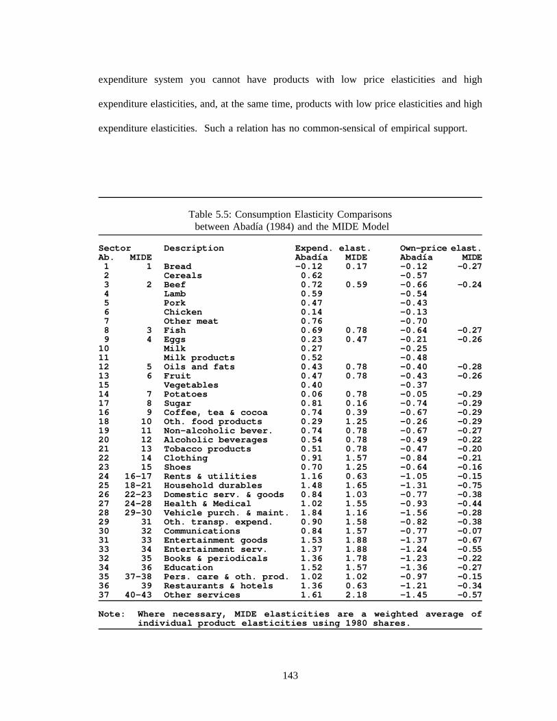
expenditure system you cannot have products with low price elasticities and high
expenditure elasticities, and, at the same time, products with low price elasticities and high
expenditure elasticities. Such a relation has no common-sensical of empirical support.
Table 5.5: Consumption Elasticity Comparisonsbetween Abadía (1984) and the MIDE Model
Sector Description Expend. elast. Own-price elast.Ab. MIDE Abadía MIDE Abadía MIDE1 1 Bread -0.12 0.17 -0.12 -0.272 Cereals 0.62 -0.573 2 Beef 0.72 0.59 -0.66 -0.244 Lamb 0.59 -0.545 Pork 0.47 -0.436 Chicken 0.14 -0.137 Other meat 0.76 -0.708 3 Fish 0.69 0.78 -0.64 -0.279 4 Eggs 0.23 0.47 -0.21 -0.26
10 Milk 0.27 -0.2511 Milk products 0.52 -0.4812 5 Oils and fats 0.43 0.78 -0.40 -0.2813 6 Fruit 0.47 0.78 -0.43 -0.2615 Vegetables 0.40 -0.3714 7 Potatoes 0.06 0.78 -0.05 -0.2917 8 Sugar 0.81 0.16 -0.74 -0.2916 9 Coffee, tea & cocoa 0.74 0.39 -0.67 -0.2918 10 Oth. food products 0.29 1.25 -0.26 -0.2919 11 Non-alcoholic bever. 0.74 0.78 -0.67 -0.2720 12 Alcoholic beverages 0.54 0.78 -0.49 -0.2221 13 Tobacco products 0.51 0.78 -0.47 -0.2022 14 Clothing 0.91 1.57 -0.84 -0.2123 15 Shoes 0.70 1.25 -0.64 -0.1624 16-17 Rents & utilities 1.16 0.63 -1.05 -0.1525 18-21 Household durables 1.48 1.65 -1.31 -0.7526 22-23 Domestic serv. & goods 0.84 1.03 -0.77 -0.3827 24-28 Health & Medical 1.02 1.55 -0.93 -0.4428 29-30 Vehicle purch. & maint. 1.84 1.16 -1.56 -0.2829 31 Oth. transp. expend. 0.90 1.58 -0.82 -0.3830 32 Communications 0.84 1.57 -0.77 -0.0731 33 Entertainment goods 1.53 1.88 -1.37 -0.6733 34 Entertainment serv. 1.37 1.88 -1.24 -0.5532 35 Books & periodicals 1.36 1.78 -1.23 -0.2234 36 Education 1.52 1.57 -1.36 -0.2735 37-38 Pers. care & oth. prod. 1.02 1.02 -0.97 -0.1536 39 Restaurants & hotels 1.36 0.63 -1.21 -0.3437 40-43 Other services 1.61 2.18 -1.45 -0.57
Note: Where necessary, MIDE elasticities are a weighted average ofindividual product elasticities using 1980 shares.
143

5.2 Fixed Capital Investment
Non-residential Investment
The most important economic event in Spain from 1985 through 1989 was the rapid
expansion of fixed capital investment. Table 5.6 displays the average annual growth rates
of the ten categories of non-residential investment enumerated in the MIDE model. The
figures are divided into four, five-year periods: 1970-74, 1975-79, 1980-84 and 1985-89.
It is clear that, after a period of stagnation from 1975 through 1984, capital spending for
eight of the commodities expanded vigorously after 1984. Commentators offer several
explanations for this extraordinary growth (see, for example, González-Romero and Myro,
1989). Much of it is attributed to exogenous factors related to the entry of Spain into the
EC. In Chapter 2, I cited several arguments why Spain’s entrance into the EC stimulated
both domestic and foreign direct investment. These points deserve repeating once again:
1) Once EC membership was assured, foreign investors perceived theadvantage of gaining a foothold in an EC country with both low relativelabor costs and a rapidly expanding domestic market.
2) Domestic producers recognized the opportunity of expanded exportsmarkets provided by EC integration, but also the need to update theirproduction technologies in order to compete in those markets.
3) EC integration reduced uncertainty of future economic regulation. Before1986, the Spanish government played a high role in the economy,compared to the average EC government. By accepting the EC rules ofthe game, the Socialist administration demonstrated the willingness tomove forward with drastic, and permanent, liberalization. Moreimportant, it was apparent that EC membership was very popular with theSpanish people. Thus, even with a change of government attitudes,investors could be confident that future economic regulation would beless subject to the whims of the local political environment.
4) A very important aspect of the economic liberalization was a greateravailability and a reduction in the costs of imported inputs. Therefore,trade reforms raised the rate of return to capital.
144

Table 5.6: Fixed Capital Non-Residential Investment, 1970-89.(Average annual growth rates, constant 1980 prices.)
Investment product 70-74 75-79 80-84 85-89 %tot*
1. Agricultural, forestry& fishery products
2. Metal products
3. Agricultural machinery& tractors
4. Industrial machinery
5. Office mach., computers,precis. & optic. instr.
6. Electrical & electronicmachinery
7. Motor vehicles
8. Oth. transport equipment,incl. ships, planes & r.r.
9. Nonresidential construction
10. Other products
Total non-residential fixedcapital investment
3.1 -0.9 2.0 -0.2 0.4
6.0 0.1 -2.8 13.6 5.9
11.7 -8.2 -2.1 2.2 1.0
7.4 -5.9 -1.1 17.0 11.4
8.8 -0.0 10.7 16.2 4.9
15.6 0.4 3.0 12.5 9.8
4.7 7.5 -4.6 14.7 9.1
23.3 -13.4 -15.8 40.6 3.3
7.4 -1.0 -1.0 12.2 48.5
7.0 -2.8 -0.8 10.9 5.8
8.5 -1.8 -1.4 13.3 100.0
* -- Percentage of total in 1989.
5) With the help of EC regional development funds, the Spanish governmentinitiated an expanded program of infrastructure investment. (This factorappears mostly in the Other construction category.)
There are at least three other policy developments which worked to encouraged
investment. Although these policies would have probably been implemented even if Spain
had not joined the EC, membership certainly sustained their pace and momentum. The first
policy, a program of incentives to foreign investors, especially for activities in certain high
technology sectors or in regions of interest, stimulated direct capital inflow. It is difficult
145

to judge, however, whether the impact of the incentives was significant. Much of the direct
investment covered by these programs would have probably occurred even without the
incentives. A second, and more important, government policy stance concerned the labor
market. In the early 1980’s the government embarked on a program of labor market reforms
intended to decrease rigidities in the labor market. The most important reforms reduced the
fix costs of hiring and firing employees. Given the high level of Franco-style labor
regulation in the Spanish economy, these reforms were vital for stimulating investor
confidence. I will have much more to say about these reforms in the next chapter.
The third set of policies, and in my opinion the most important, were financial market
reforms that have reduced the amount of credit rationing in the economy. The changes have
been gradual, but steady. Deposit and lending rates were totally deregulated in 1987, setting
of an intense battle in retail banking. The securities markets were completely overhauled
in 1989. The "investment coefficient" (coeficiente de inversión) regulations, which obligated
banks to set aside a specified proportion of deposits for government approved investment
projects, usually for public-sector firms, have been eased and will eventually be eliminated.
The gradual liberalization of foreign capital flows to EC standards will be complete by mid-
1992. The reforms have improved investor access to credit, particularly for smaller firms.
Traditionally, these firms were the first to be squeezed for investment finance in times of
credit rationing. Capital market reforms will continue to have a large impact on the Spanish
economy.
Taken together, these influences on investment behavior present important concerns for
the estimation of the capital expenditure functions of the MIDE model. As described in the
last chapter, the MIDE model contains accelerator functions for ten different categories of
capital goods. This explanation of investment purchases assumes that net capital formation
146

is a function of past and present production in the purchasing sectors, and that replacement
investment is identical to depreciation of the capital stock. The equations will fill two roles.
One is to forecast investment through the 1990’s and the other is to simulate the history or
investment through the middle to late 1980’s. These two roles may conflict. If the recent
spectacular investment growth is only temporary phenomena related to EC entry, then
equations estimated over the period may produce parameters that perform well in historic
simulation but are inappropriate for forecasting.
Clearly, the investment explosion is not a permanent phenomena. It is unreasonable to
expect to continuation of 10 or 15 percent investment growth. Moreover, 1990 saw a
marked slow down in aggregate investment growth and 1991 saw negative growth for
equipment goods. The party is already over. Therefore, the specification of the functions
must account for the temporary, exogenous influences on investment behavior from 1985
to 1989. The equations must produce investment growth rates (i.e., have slopes) which
reflect a slow-down of investment activity. Are the correct forecasting coefficients the same
parameters displayed by the economy previous to 1985?
Important and continuing reforms in the labor, capital and foreign trade markets and the
change in the political climate have permanently changed the investment behavior of Spanish
producers. Simply assuming that investment behavior will return to its pre-1985 trends is
precarious. Since there are now fewer obstacles to implementing investment decisions,
capital expenditure should become more responsive to output growth. Ideally, we should
look for forecasting equations which display this property. At the same time, we must also
consider the econometric and historical simulations properties. The estimation process
described below addresses these issues.
Economists have devoted much work in attempting to explain the determinants of
147
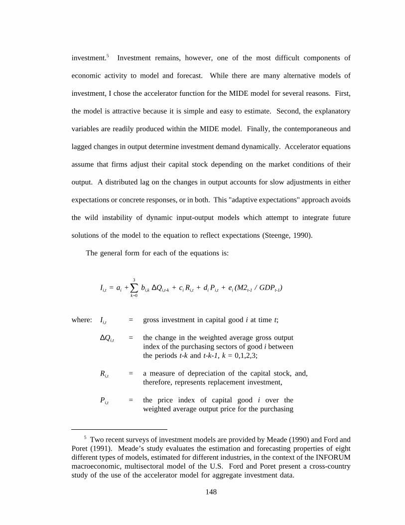
investment.5 Investment remains, however, one of the most difficult components of
economic activity to model and forecast. While there are many alternative models of
investment, I chose the accelerator function for the MIDE model for several reasons. First,
the model is attractive because it is simple and easy to estimate. Second, the explanatory
variables are readily produced within the MIDE model. Finally, the contemporaneous and
lagged changes in output determine investment demand dynamically. Accelerator equations
assume that firms adjust their capital stock depending on the market conditions of their
output. A distributed lag on the changes in output accounts for slow adjustments in either
expectations or concrete responses, or in both. This "adaptive expectations" approach avoids
the wild instability of dynamic input-output models which attempt to integrate future
solutions of the model to the equation to reflect expectations (Steenge, 1990).
The general form for each of the equations is:
Ii,t = ai + bi,k ∆Qi,t-k + ci Ri,t + di Pi,t + ei (M2t-1 / GDPt-1)3
k 0
where: Ii,t = gross investment in capital good i at time t;
∆Qi,t = the change in the weighted average gross outputindex of the purchasing sectors of good i betweenthe periods t-k and t-k-1, k = 0,1,2,3;
Ri,t = a measure of depreciation of the capital stock, and,therefore, represents replacement investment,
Pi,t = the price index of capital good i over theweighted average output price for the purchasing
5 Two recent surveys of investment models are provided by Meade (1990) and Ford andPoret (1991). Meade’s study evaluates the estimation and forecasting properties of eightdifferent types of models, estimated for different industries, in the context of the INFORUMmacroeconomic, multisectoral model of the U.S. Ford and Poret present a cross-countrystudy of the use of the accelerator model for aggregate investment data.
148

sectors;
M2t = the money supply, M2, and
GDPt = nominal GDP.
The inclusion of the relative price variable adds neoclassical content since it integrates
the prices of production inputs, including labor, into the purchasing decision. The lagged
ratio of the money supply (M2) over nominal GDP accounts for financial conditions. This
"money availability" variable is invariably superior to interest rates in the Spanish equations,
presumably because of the substantial amount of credit rationing, capital controls and interest
rate regulation that have dominated the economy. As I have argued above, however, these
influences should have less influence in the future. Nevertheless, the most important
underlying determinant of real interest rates, and therefore, financial conditions, is the money
supply. In every equation the lagged money availability strongly outperformed the
contemporaneous value, illustrating the lagged effects of monetary policy. Therefore, the
specification includes only the lagged availability.
The replacement investment variable is formed assuming that physical depreciation is
a constant proportion of the capital stock. No information exists on the service lives of
capital equipment in Spain. In forming the capital stock variable for the MOISEES model,
the builders assumed a depreciation rate of ten percent per year (Corrales and Taguas 1989;
Andres et al. 1988b). This figure seems quite high for certain types of capital, especially
buildings. For office machinery and computing equipment, on the other hand, ten percent
is probably low. For disaggregated modeling, the depreciation rates should vary. The rates
used in this study are primarily intuitive estimates which straddle the ten percent figure.
They vary from 6 percent per year for Non-residential construction and the non-electric
149

machinery categories to fifteen percent per year for Office equipment and computers.
Further evaluation of the chosen rates was done in the equation estimation process.6 The
replacement variables (Ri,t) and capital stocks (Ki,t) for each commodity are constructed from
the investment series (Ii,t) using the following identities:
Ri,t = (di × Ki,t-1)
Ki,t = (1 - di) × Ki,t-1 + Ii,t
where di is the depreciation rate for capital good i.
The MIDE model contains equations of this type for the ten categories shown in Table
5.6. This classification corresponds to the national accounts 1980 based data. The accounts
provide current price series from 1980 through 1989 for each of the products, and constant
price series for five categories: Agricultural products (Commodity 1), Machinery products
(Commodities 2-6), Transport material (7-8), Non-residential construction (9) and Other
products (10). Data previous to 1980 exists in constant and current prices for only 3
categories of goods: Machinery and other products (1-6 and 10), Transport material, and
Non-residential construction. These series have been homogenized and extended back to
1954 by Corrales and Taguas (1989).
The first item to note about the 10 disaggregated series is their close correspondence
with production sectors of the input-output table. With the exception of category 10, Other
products, each commodity is manufactured by only one industry. This direct correspondence
simplifies the construction of a matrix which allocates the quantities demanded to the
6 Since the a priori value for the parameter ci is 1.00, an intuitive depreciation rate whichresults in the closest parameter estimation to this value, and which also produces reasonableestimates for the other parameters, is judged to be superior to others. In reality, there isusually little difference to the estimated parameters for the range of depreciation rates whichwould be considered realistic.
150

production sector (referred to in Chapter 4 as the B matrix). However, since the investment
series are in purchaser prices, they include commercial margins, transportation costs and
services provided by five other input-output industries. To create the B matrix, these mark-
ups were allocated to the respective service sectors using information on the construction of
the 1980 IO table provided by INE (see Sanz 1989).
The information provided by the share matrix allowed the construction of a price for
each product using the production and import prices from the corresponding input-output
sectors. Constant prices series for the products were then estimated for the years previous
to 1980, by using the aggregate investment quantities and the relevant production sector
domestic demand as indicators. While the regression period is 1969 through 1989, it is
necessary to have estimations extending back to 1954 to construct estimations of capital
stock and depreciation for each product. The Appendix provides details on the derivation
of this data.
The next step was to construct indices for the changes in output and producer prices for
the purchasing sectors. The only data of this nature available at present for the Spanish
economy is a series of capital investment matrices, covering the years 1980 through 1983,
constructed by Antón and Escribano (1988). These matrices show the flows of investment
sales from the type of product to the purchasers, classified according to the 40 non-
government sectors of the 1980 IO table. This information was converted to a coefficient
matrix for each year by dividing the demand by purchaser by the total sales by product. The
coefficients were then averaged over the period. The resulting coefficients show, albeit
roughly, the share of sales for each product demanded by each of the 40 producing sectors.
For example, the Agriculture sector makes up 94 percent of the demand for Agricultural
machinery; the Communications sector exerts a high influence for purchases of Electric and
151
Electronic equipment. The variable Qi,t was formed by multiplying the share coefficient for
each of the purchasing sectors by their respective production, indexed to be equal to 100 in
1980. The price deflator for the purchasing sectors was constructed in the same fashion.
This procedure proved to be very satisfactory for the estimation of equations.
To determine the most robust specifications, the equations were estimated for several
variations of the general form and under three different regression intervals, from 1969
through 1989, from 1969 through 1984 and from 1980 through 1989. If required, the Almon
technique for smoothing distributed lags was used on the accelerator variables, and the
coefficient on the replacement variable was softly constrained to be equal to one. This
exercise revealed the appropriate length and structure (quadratic or linear) of the distributed
lag on output change, the best depreciation rate, and the relevance of including the money
availability and the relative price variables (i.e., did they provide significant and reasonable
coefficients). Comparison between the 1969-89 and 1969-84 equations also provided the
opportunity to compare the performance of the equations for within-sample and out-of-
sample simulations and to attain an understanding of how much of the rapid growth from
1985 through 1989 could be attributed to the explanatory variables of the functions. The
results were not encouraging. Figure 5.3 displays regression fits (in billions of 1980
pesetas), a graph of coefficient estimates and summary regression results for Industrial
machinery (Commodity 4). The following discussion will progressively refer to and explain
the information on this figure in order to illustrate the general regression results by way of
a typical, and important, example.7
7 The first category, Agricultural products investment (mostly livestock), is excludedfrom this discussion since it is a rather special case. The equation estimated for 1969-89handles this series satisfactorily. Moreover, since it is a trivial figure (0.4 percent of totalnon-residential investment in 1989) there is no need to devote any further space to adescription of its equation.
152

Estimations for the regression interval of 1969-84 produced reasonable econometric
results, but failed miserably in predicting the actual 1985-89 data. For seven of the
products, Chow tests conducted for the 1969-84 and 1969-89 intervals produced significant
F-statistics. This is evidence of structural change. In general, the 1969-89 estimations fit
the data fairly well (in terms of RBSQ), but they also underestimated investment for 1985-89
(Figure 5.3). Some are much worse than others in this respect. As could be expected, the
equations estimated from 1980-89 produced terrific fits to the data. However, in some of
the categories, the loss of observations played havoc with the parameter values. In others,
the accelerator parameters were so high that they would be explosive for forecasting (see the
regression coefficient plot in Figure 5.3).
Another problem for some of the 1969-89 equations was their tendency to place the
bulk of the explanatory power in the replacement terms with unconstrained parameters taking
values much greater than 1.0 (1.3 - 2.0). While it was easy to softly constrain the 1969-84
replacement parameters to be 1.0, the 1969-89 estimates were particularly stubborn.
Progressively harder constraints produced substantial autocorrelation and began to affect the
other coefficients, producing unreasonable values. Despite these problems, the 1969-89
estimations were satisfactory enough to allow their use for forecasting equations of the
MIDE model. The coefficients of the equations are between the 1969-84 (sluggish) and
1980-89 (explosive) values (Figure 5.3). While this is a desirable property for forecasting,
the regression plot shows that the 1969-89 equation would produce lousy historic simulations
for 1985-89. Obviously, there is something missing in the equations that would enable an
accounting for the above cited exogenous influences on investment between 1985-89.
153

Figure 5.3: Summary Regression Results for Investment inIndustrial machinery (4)
Predicted vs. Actual, 1969-89
Regression coefficients (depr. rate = 6%)
dQt dQt-1 dQt-2 dQt-3 repl. relpr. M2/GDP
equation see mape rbsq rho t-stat1969-84 8.72 2.84 .857 -.351980-89 15.42 4.64 .859 .301969-89 32.34 8.02 .631 .781969-89 w/dummy 22.53 5.68 .806 .45 1.921969-89 w/trend 9.32 2.84 .967 .23 9.04
1969-89 1969-89 w/dum 1969-89 w/trend
Economet./Hist.Sim. results poor fair good
Forecast growth rate high medium low
Final equation choice: 1969-89, w/trend
154

One alternative is to add a simple dummy variable to the 1969-89 regressions for the
years 1985 through 1989.8 This is equivalent to assuming that the intercept of the function
changed. For most of the equations, this approach yielded more satisfactory results. For
others, however, the fits and historical simulation performance for 1985-89 are not
particularly better than the other 1969-89 equations. To return to the example of Industrial
machinery, the within-sample 1985-89 predictions of this equation are superior to the
equation which does not include the dummy (Figure 5.3). However, we would not trust this
equation to produce good historical simulations. The equations also required relatively hard
constraints to obtain a value of 1.0 for the replacement parameter, with the accompanying
autocorrelation problem. The inclusion of the dummy does produce accelerator coefficients
which lie below the 1969-89 estimates, but above the 1969-84 values.
Another issue must be addressed: if we are to use intercept dummies for the forecasting
equations, what value should the dummy take on in the forecast (i.e., post 1989) period for
predictions of the full model? Since the dummy represents exogenous factors, the answer
depends on how we perceive these influences will change in the forecast period. Since
integration in the EC and the wider availability of financing will continue to affect
investment in the future, it is appropriate to keep the dummy variable at its 1987 value
indefinitely. However, assuming a general growth trend for each of the investment series,
the proportional effect of the dummy will decrease through time. This is a desirable
property. It reflects that changes in the environment initiated in 1985 will exert a decreasing
effect on investment through time.
8 The dummy variable is specified as equal to .5 in 1985, 1 for 1986-89, and 0 for allother years. The differential between 1985 and the other years reflects that fact that theexogenous factors cited at the beginning of the section became important only in the secondhalf of 1985.
155
Another option for estimating the functions is to change the slope of the equation by
inserting a time trend that begins in 1985.9 This solves several estimation problems, not
to mention the historic simulation difficulties. The fit for 1985-89 is excellent. The
pressure on the replacement parameter disappears, hard constraints are no longer needed to
obtain a value of 1.0. The accelerator parameters, more or less, revert to their values from
the 1969-84 regressions (Figure 5.3). Consequently, this technique introduces an important
forecasting question: What happens to the trend after 1989? If it continues along it’s merry
way, the model assumes that the extraordinary behavior of 1985-89 continues, a fact we
know is not correct. An alternative is to fix the trend at its 1989 value. Note that this is
equivalent to assuming that the investment behavior reverts to the sluggish pre-1985
behavior, a dubious assumption. A third possibility is to allow the trend variable to grow,
but at a decreasing rate. While this option places much of the forecast burden onto the
assumptions of the forecaster, it will often lead to the most realistic projections. I will have
more to say about this presently.
To summarize, there are three possibilities to choose from: the 1969-89 equation (1969-
89), the 1969-89 equation with the EC slope dummy (1969-89 w/dummy), and the 1969-89
equation with the EC time trend (1969-89 w/trend). The choice among the alternatives
often involves stark tradeoffs among econometric results, historical simulation performance
and forecasting properties. The dilemma for Industrial machinery is summarized by the
regression results and "comparison matrix" displayed at the bottom of Figure 5.3. The
regression results display the standard error of the estimate (see), the mean absolute
percentage error (mape), the R-bar-squared (rbsq), the autocorrelation of the residuals (rho)
9 The time trend variable is specified as equal to .5 in 1985, 1 for 1986, 2 in 1987, 3in 1988 and 4 in 1989. Again, the peculiar 1985 value is due to that fact that the exogenouspositive influences on investment were important from the second half of 1985.
156

and the t-statistic on the dummy or trend coefficient (t-stat) where it applies. In this
example, the "1969-89 w/trend" equation displays superior econometric and historical
simulation properties.10 This result is noted in the line of the comparison matrix labelled
"Economet./Hist.Sim. results."11 As illustrated by the "Forecast growth rate" line, each
equation assumes a different underlying, forecast growth rate of investment. Once we admit
this item into the utility function, we choose among somewhat arbitrary assumptions
concerning investment behavior. In this case, I have inserted the "1969-89 w/trend" equation
into the MIDE model because of its better econometric performance and the high
significance of the time trend. Also, forecasts for Industrial machinery investment with the
time trend frozen at its 1989 value are not unduly pessimistic but seem rather plausible.
Unfortunately, the choice among equation forms must be made for each category. For
example, for Office machines, computers and precision instruments, the "1969-89 w/dummy"
equation displays better econometric results than the trend equation. The dummy is
significant, while the trend is not (Figure 5.6). Therefore, I have selected the dummy
equation for computers.
Figures 5.4 through 5.11 display the results and equation selection for each of the other
categories. I have made the selections with more or less equal weighting toward the
sensibility of the coefficient estimates, the econometric and historic simulation performance,
and the suitability of forecasts. Although less important, the statistical significance of the
dummy or trend variables is also considered. For example, the high t-statistics on the time
10 In terms of historic simulation properties, I am primarily concerned with the 1985-89period, since the MIDE model will rarely be used for earlier periods.
11 The terms in this and the following comparison matrices are relative only among thethree equations being compared. There is no consideration given to the 1980-89 or 1969-84equations, nor is there any attempt to compare equation results across products.
157

trend coefficients reinforces the choice of trend equations for Metal products (category 2),
Industrial machinery (4) and Motor vehicles (7). On the other hand, the Electric and
electronic machinery sector (6) uses the dummy equation where the dummy is not significant
and does not contribute to the improvement of the regression statistics. A close scrutiny of
the coefficient plot reveals that this equation provides more moderate and reasonable values.
Furthermore, the dummy allowed a much softer constraint on the replacement parameter.
Certainly, I have injected a large amount of subjective judgement into the determination
of these investment functions. Since the general economic growth projected by the MIDE
model depends heavily on the growth of investment, the choices made here will determine
the forecasts to a large extent, even before they are run. Moreover, with the open possibility
of manipulating the exogenous time trend the forecaster can further inject his personal views
into forecasts.12 This can be understandingly troubling for the reader. He should be aware,
however, that this "eclectic econometric" approach is standard practice in macroeconomic
models used for forecasting. Indeed, model building would be quite impossible without this
approach. In a recent commentary on macro-forecasting, Zarnowitz (1991) makes this clear.
He cites a variety of surveys which shows that forecasters use a large amount of subjective
opinion in making projections, and that even those that rely primarily on large-scale
empirical models use a significant amount of judgement to modify these models (pp. 7-10).
The determination of capital expenditures for the MIDE model illustrates a typical
application of the discretionary techniques of empirical model construction.
12 All of the forecasts presented in Chapter 8 have the time trend frozen at 1989 level.
158

Figure 5.4: Summary Regression Results for Investment inMetal products (2)
Predicted vs. Actual, 1969-89
Regression coefficients (depr. rate = 6%)
dQt dQt-1 dQt-2 dQt-3 repl. M2/GDP
equation see mape rbsq rho t-stat1969-84 5.33 2.87 .715 .541980-89 15.64 5.74 .420 .581969-89 18.85 7.77 .478 .861969-89 w/dummy 11.99 4.78 .773 .62 2.641969-89 w/trend 4.77 2.47 .964 .36 8.15
1969-89 1969-89 w/dum 1969-89 w/trend
Economet./Hist.sim. results poor fair good
Forecast growth rate high low lowest
Final equation choice: 1969-89, w/trend
159

Figure 5.5: Summary Regression Results for Investment inAgricultural machinery (3)
Predicted vs. Actual, 1969-89
Regression coefficients (depr. rate = 6%)
dQt dQt-1 dQt-2 dQt-3 repl. relpr. M2/GDP
equation see mape rbsq rho t-stat1969-84 3.76 6.63 .706 .461980-89 1.18 2.57 .512 .001969-89 4.15 7.51 .662 .511969-89 w/dummy 3.38 5.81 .757 .47 2.461969-89 w/trend 3.77 7.05 .698 .52 1.59
1969-89 1969-89 w/dum 1969-89 w/trend
Economet./Hist.sim. results fair fair fair
Forecast growth rate little practical difference higher
Final equation choice: 1969-89, w/dummy
160
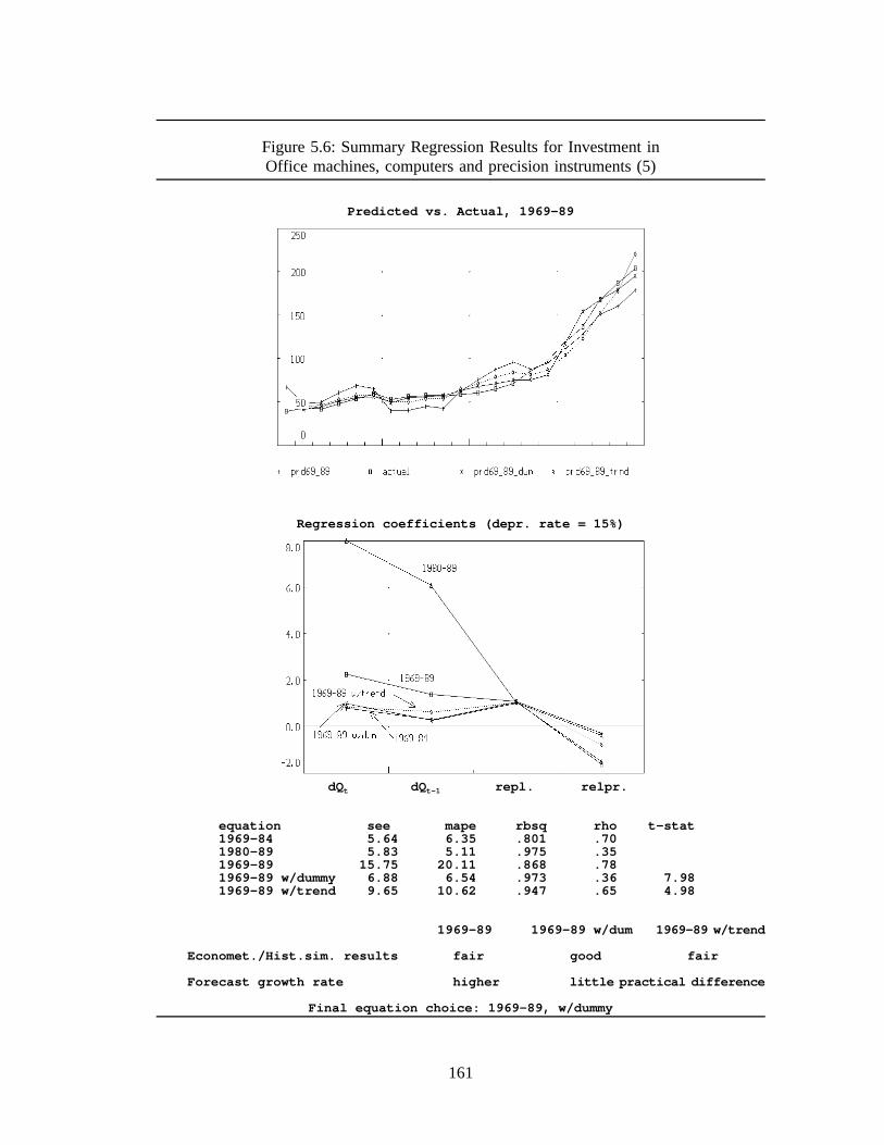
Figure 5.6: Summary Regression Results for Investment inOffice machines, computers and precision instruments (5)
Predicted vs. Actual, 1969-89
Regression coefficients (depr. rate = 15%)
dQt dQt-1 repl. relpr.
equation see mape rbsq rho t-stat1969-84 5.64 6.35 .801 .701980-89 5.83 5.11 .975 .351969-89 15.75 20.11 .868 .781969-89 w/dummy 6.88 6.54 .973 .36 7.981969-89 w/trend 9.65 10.62 .947 .65 4.98
1969-89 1969-89 w/dum 1969-89 w/trend
Economet./Hist.sim. results fair good fair
Forecast growth rate higher little practical difference
Final equation choice: 1969-89, w/dummy
161
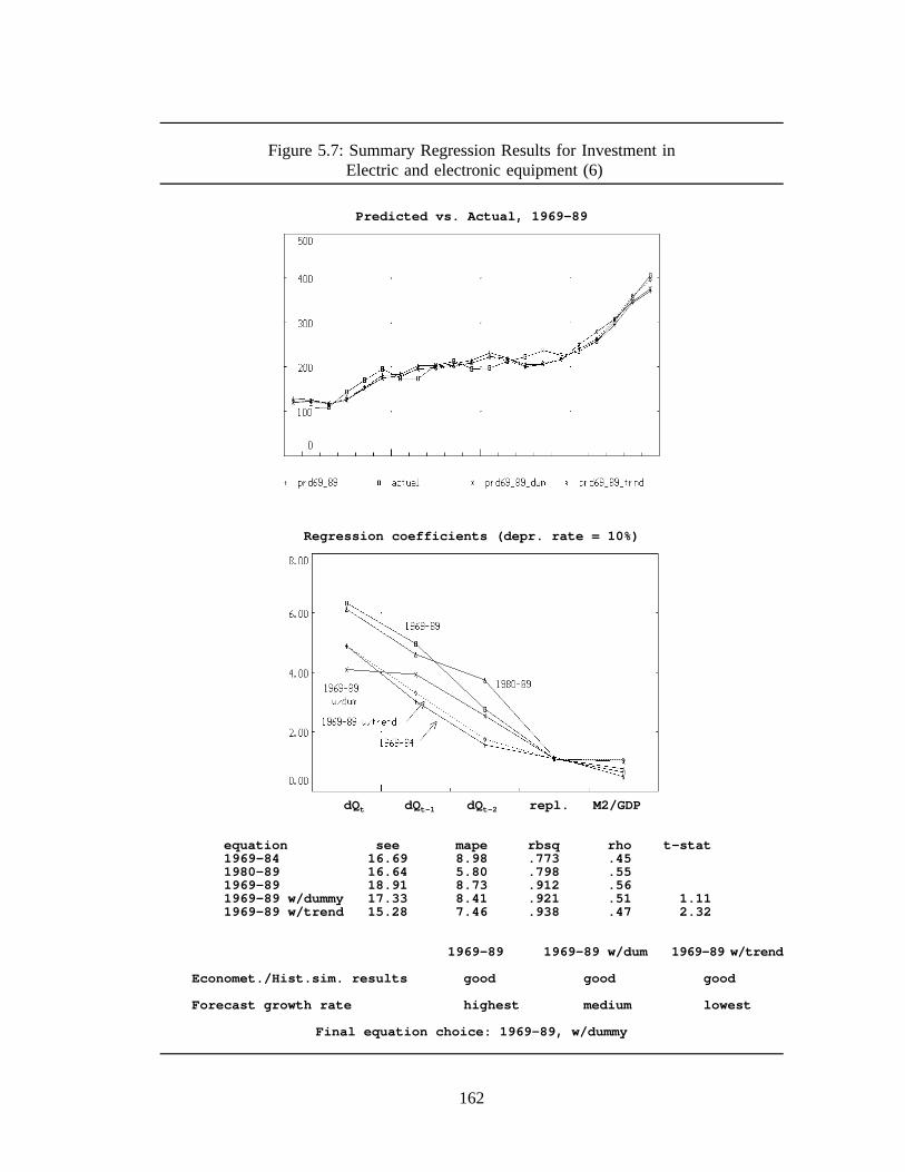
Figure 5.7: Summary Regression Results for Investment inElectric and electronic equipment (6)
Predicted vs. Actual, 1969-89
Regression coefficients (depr. rate = 10%)
dQt dQt-1 dQt-2 repl. M2/GDP
equation see mape rbsq rho t-stat1969-84 16.69 8.98 .773 .451980-89 16.64 5.80 .798 .551969-89 18.91 8.73 .912 .561969-89 w/dummy 17.33 8.41 .921 .51 1.111969-89 w/trend 15.28 7.46 .938 .47 2.32
1969-89 1969-89 w/dum 1969-89 w/trend
Economet./Hist.sim. results good good good
Forecast growth rate highest medium lowest
Final equation choice: 1969-89, w/dummy
162

Figure 5.8: Summary Regression Results for Investment inMotor vehicles (7)
Predicted vs. Actual, 1969-89
Regression coefficients (depr. rate = 10%)
dQt dQt-1 dQt-2 dQt-3 repl. relpr. M2/GDP
equation see mape rbsq rho t-stat1969-84 16.62 7.81 .609 .681980-89 8.55 3.22 .915 -.351969-89 25.58 10.87 .746 .711969-89 w/dummy 21.93 9.00 .798 .66 2.251969-89 w/trend 17.67 7.55 .869 .57 4.41
1969-89 1969-89 w/dum 1969-89 w/trend
Hist. simul. performance fair fair good
Forecast growth rate highest low lowest
Final equation choice: 1969-89, w/trend
163

Figure 5.9: Summary Regression Results for Investment inOther transport machinery (8)
Predicted vs. Actual, 1969-89
Regression coefficients (depr. rate = 6%)
dQt dQt-1 dQt-2 dQt-3 repl. relpr. M2/GDP
equation see mape rbsq rho t-stat1969-84 23.25 18.82 .589 .521980-89 21.50 23.75 -.404 .201969-89 27.30 24.59 .577 .561969-89 w/dummy 24.12 22.38 .642 .56 1.931969-89 w/trend 20.85 15.88 .733 .50 3.00
1969-89 1969-89 w/dum 1969-89 w/trend
Economet./Hist.Sim results fair poor good
Forecast growth rate highest medium lowest
Final equation choice: 1969-89
164

Figure 5.10: Summary Regression Results for Investment inNon-residential construction (9)
Predicted vs. Actual, 1969-89
Regression coefficients (depr. rate = 6%)
dQt dQt-1 dQt-2 dQt-3 repl. relpr. M2/GDP
equation see mape rbsq rho t-stat1969-84 17.37 1.09 .951 -.391969-89 57.32 3.72 .906 .471980-89 27.75 1.77 .952 -.131969-89 w/dummy 57.10 3.59 .899 .47 0.631969-89 w/trend 27.32 1.41 .977 .10 4.76
1969-89 1969-89 w/dum 1969-89 w/trend
Hist. simul. performance good good good
Forecast growth rate little practical difference low
Final equation choice: 1969-89
165

Figure 5.11: Summary Regression Results for Investment inOther products (10)
Predicted vs. Actual, 1969-89
Regression coefficients
dQt dQt-1 dQt-2 dQt-3 repl. M2/GDP
equation see mape rbsq rho t-stat1969-84 5.06 3.00 .791 .371980-89 4.29 2.27 .956 -.581969-89 6.50 3.53 .929 .301969-89 w/dummy 5.98 3.16 .936 .32 1.251969-89 w/trend 5.52 2.98 .945 .19 1.92
1969-89 1969-89 w/dum 1969-89 w/trend
Hist. simul. performance good good good
Forecast growth rate highest medium lowest
Final equation choice: 1969-89, w/dummy
166

Residential Construction
Residential construction is estimated in per capita terms. The equation contains three
explanatory factors: disposable income per capita, the stock of housing per capita, and a
three year moving average of the M2 over nominal GDP ratio. The underlying concept of
the function is that the desired consumption of houses depends on disposable income (Y),
and that the investment (I) depends on the difference between this desired consumption and
the actual consumption level (K) (Almon 1988, pp.201-2):
I = (a + bY) - K
The influence of the income level will apply with a lag because of the permanent income
effect and adjustment costs. Additionally, consumers are constrained by financial conditions.
Historically, interest rates have exerted little influence in the market. The availability of
money is much more effective in the equation. The full functional form of is:
It = a + bYt-1 + ck∆Yt-k + dKt + e wk (M2t-k /GDPt-k )2
k 0
2
k 0
where: It = per capita gross investment housing at time t,
Yt-1 = per capita real personal disposable income,
∆Yt-k = changes in per capita real disposable incomebetween periods t-k and t-(k-1), k = 0, 1, 2,
Kt = a measure of housing stock per capita,
M2t = the money supply, M2,
GDPt = nominal GDP, and
wk = .3, .5, .2 for k = 0, 1, 2, respectively.
The housing stock was constructed in the same fashion as the non-residential stocks
167

with a depreciation rate of 3.3 percent per year. The coefficient on this variable, d, was
softly constrained to take on the value of negative one as demanded by the theory. The
coefficients on the distributed lag on changes in income were constrained to lie on a straight
line. The constraints required were extremely light. Figure 3.12 displays the results for two
regression intervals: 1970-89 (the MIDE model equation) and 1970-84. All of the
parameters exhibit the correct signs and reasonable values. Moreover, they are remarkably
stable between the two regression periods. Both equations fit very well and the ex-post
forecast for the 1970-84 equation, while systematically over-shooting the actual values,
tracks them nicely. The results are all the more satisfactory when one considers the
importance of residential construction in the economy, and therefore, in the MIDE model.
However, the equation must be used with care for forecasting. The retail banking
reforms now taking place in the Spanish economy should have a particularly marked impact
in the housing market. In 1991, long-term mortgages which would finance a majority of the
cost of a new home appeared for the first time. Moreover, foreign banks will increasingly
become a source of housing loans. One outcome of these changes will probably be a greater
influence of the interest rate on housing construction. It is impossible to judge the impacts
of the banking changes given the available data. However, as stated earlier in the chapter,
because money availability plays the most important role in determining the interest rate, the
present equation is responsive to credit conditions and will likely yield satisfactory
predictions.
168

Figure 5.12: Summary Regression Results forResidential construction, 1970-89.
Actual vs. Predicted Values.(thousands of 1980 pesetas per capita)
1970-89SEE = 0.57 RHO = 0.15RBSQ = 0.98 DW = 1.69MAPE = 1.76
Variable name Reg-Coef t-value Meanresid. const. pc - - - - - - - - - 26.38intercept -0.966 -0.27 1.00Ypc(t-1) 0.065 6.96 284.93dYpc 0.065 * 5.66dYpc(t-1) 0.043 * 5.71dYpc(t-2) 0.024 * 5.30housing stock -1.010 * 21.96M2/GDP 3-yr mov avg 0.590 20.02 51.16
* - denotes restricted coefficient
1970-84SEE = 0.59 RHO = 0.17RBSQ = 0.96 DW = 1.65MAPE = 1.77
Reg-Coef t-value Mean- - - - - - - - - 27.82
0.121 0.03 1.000.068 4.22 279.240.074 * 4.080.052 * 5.110.026 * 5.85-1.012 * 21.920.558 6.955 54.31
Test period (1985-89):SEE = 0.78 MAPE = 3.15
169

CHAPTER 6:
ECONOMETRIC SPECIFICATION AND ESTIMATES:
FOREIGN TRADE, PRODUCTIVITY AND EMPLOYMENT
6.1 International trade
As a small country, international trade is very important to Spain. In 1990 the current
price imports to GDP ratio was 20.9 percent; the export to GDP ratio was 17.6 (figures
include tourism). Trade played an important role in the modernization of the Spanish
economy. As Dehesa et al. (1988) reported, spurts in growth for the Spanish economy were
highly correlated with high trade growth. Between 1960 and 1974, when the real economy
expanded at an average of 6.9 percent per year, real imports expanded at an average rate of
16.4 percent per year, and exports grew at 14.9 percent per year. Between 1975 to 1985,
the corresponding figures were 1.9 percent for imports and 6.6 percent for exports as GDP
grew by only 1.5 percent. Recent years, however, present a more mixed picture. From
1986 through 1990, while average GDP growth registered 4.5 percent, imports rose by 15.2
percent per year, but exports grew only 4.9 percent per year. Since this period coincides
with Spain’s membership in the European Community, the future direction of foreign trade
under increasing integration has become a major question concerning the Spanish economy.
Starting in 1993, intra-EC merchandise trade will be completely free, and service trade
will become more liberalized as time goes by. Additionally, Spanish trade barriers with the
rest of the world will be further reduced for many key categories of goods and services, as
Spain harmonizes its trade policy with that of the EC. For example, under a recent
agreement between the EC Commission and Japan, Spanish import quotas for Japanese made
automobiles, now a miserly two percent, will gradually increase to around ten percent by
170

1999 (Economist June 8, 1991, p.25). This additional liberalization will occur when Spain
is already sustaining enormous trade deficits. Consequently, an extensive discussion over
whether the Spanish economy can compete in international markets has dominated economic
discussion over the past few years.1
Chapter 2 discussed the role of international trade in the history and future of the
economy and outlined some sectoral trends for imports and exports. It is helpful to recall
some of these points here:
1) Disequilibriums in the trade balance has often stymied the growth of theSpanish economy. Since joining the EC in 1986, imports have increasedrapidly, but exports increases have been disappointing. Possible explanationsinclude the higher income price and wage growth rates of Spain relative to itsEC partners, reduction of Spanish trade barriers, and the steady appreciationof the peseta since integration. Also, substantial inflows of direct foreigninvestment since 1985 have stimulated a direct flow of imports.
2) At the sectoral level, high demand elasticities for imports, especially forinvestment goods, insure a deteriorating trade balance as soon as growth getsunder way. In some industries, strong domestic demand growth divertspotential exports toward the domestic market, further aggravating tradedeficits.
3) In industries that are labor intensive (textiles, toys) or resource intensive (fruitand vegetables), Spain appears to have a comparative advantage vis-á-vis theEC. However, strong competition in these areas can be expected fromdeveloping and formerly centrally planned economies. In many high growthindustries, such as electronics, Spanish industry suffers a comparativedisadvantage. Many Spanish service industries also seem vulnerable.
4) Presently, most of Spain’s best export performances are registered by firmsdependent on foreign capital, technology and marketing resources. Two keysectors, automobiles and computers, are cases in point.
5) While it is too early to judge, it is possible that the growth of the mighty Spanishtourist industry may come to a halt. The sector must accommodate domestic priceincreases and changing consumer tastes to remain the foundation of Spanish
1 For a review of this discussion, see the collection of nine articles by the majorcommentators entitled "Commercial Deficit and Competiveness," in the magazine 3conomi41990, 5.
171

exports.
In order to project a future path for imports and exports, it is helpful to access the
relative importance of the above points. Interestingly, several commentators have asserted
that EC membership produced a fundamental structural change in foreign trade (an argument
similar to that made in the last chapter on investment). These observers maintain that this
structural change has increased the underlying propensity to import, but left unchanged the
export potential, boding poorly for the future of the Spanish trade balance (see, for example,
Martínez, Sanso and Sanz 1991; Martínez and Montañes 1991; Montes 1988). The
econometric estimation of the aggregate import and export functions of the MOISEES model
shed light on this issue (Fernandez and Sebastián 1990a, 1990b and 1989; Manzanedo and
Sebastián 1989). In general, Fernandez and Sebastián reject the hypothesis of EC-induced
structural change. Their work shows, instead, that equations estimated over the period of
1964-88 for non-energy imports (excluding tourism), energy imports, and exports (again
excluding tourism) are relatively stable through time. Using a "dynamic structural
approach," which included error correction mechanisms based on cointegration techniques,
they obtained the following conclusions:
1) Non-energy imports were significantly influenced by changes in investmentas well as the level of GDP, the relative price and domestic capital utilization.Using dummy variables to detect both one-time and long-term structuralchanges in the parameters of the equations, they found no evidence of ECentry induced structural change for non-energy imports. Fernandez andSebastián found that domestic activity and relative prices could notsatisfactorily explain energy imports. The behavior of energy imports since1986 have been quite strange, increasing slowly despite large falls in price anda rapidly expanding economy. In 1988, the volume of energy imports actuallyfell. According to Fernandez and Sebastián, the uncertainty of the oil marketled to a large accumulation of oil stocks when the expected future price wasmuch larger than the actual price in the early 1980’s. When theseexpectations were not met, refiners reduced the stocks and imported less.
172
Therefore, Fernandez and Sebastián included a variable for the accumulatedchanges in relative prices to represent the expectations of future prices andobtained a better equation.
2) Over the long run, Spanish exports of good and services can be explainedalmost completely by variations in commercial indexes, that is, foreigndemand. However, a loss in price competiveness since 1983 has significantlyreduced the growth rate of exports. A negative impact of domestic demandpressure on exports, while statistically significant, is minor. Finally,Fernandez and Sebastián did find some evidence of structural change,represented by a significant and negative intercept changing dummy, forexports from 1986. However, the temporary dummy (i.e., equaling 1 in 1986and 0 elsewhere) was slightly more important compared to a permanentdummy (equaling 1 in 1986 to 1988 and 0 elsewhere), leading the authors tosuspect that the changes will be temporary. They gave several potentialreasons for such a short run change, including the loss of direct exportsubsidies prohibited by EC policy, and the loss of indirect export subsidiesexperienced because of the change of indirect tax regime.2
This work suggests that the recent behavior of aggregate international trade can be
explained by the more traditional factors of relative demands and prices. But they also leave
many questions open. Often, an aggregate analysis can hide changes in the trade
environment that affect individual industries quite significantly. Moreover, they tell us
nothing of the composition of trade and where the comparative advantage of the Spanish
economy lies. For both imports and exports, there is no elaboration of which sectors are
relatively demand sensitive and which are price sensitive. These questions are very
important for the prospects of individual industries. They require a disaggregated
examination of foreign trade. Except for work done by Carmela Martín and her colleagues
2 Previous to EC entry, the Spanish indirect tax regime was a cascade tax which fellon all sales, including intermediate consumption. When goods were exported, the exportersreceived a refund of the taxes paid on intermediate inputs. In practice, the refund ordesgravación fiscal a la exportación (DFE), resulted in an indirect export subsidy becausethe refund was not available if the goods were sold domestically. Moreover, the refund wasoften greater than the amount of taxes actually paid. This system was replaced by a valueadded tax (VAT) in 1986. Under the VAT, taxes paid on intermediate inputs are refundedwhether sold domestically or exported.
173

at Fundación Empresa Pública (see, for example, Martín and Moreno 1990; Martín, 1990a;
and Martín, et. al. 1987), and this only for manufacturing trade, research in Spain has not
touched a sectoral analysis of international trade.
A Sectoral Analysis of Spanish Foreign Trade
The following describes the estimation of the import and export equations of the MIDE
model. Since the model links the Spanish economy to most of its major trading partners at
the sectoral level through the INFORUM international system, it provides a particularly good
vehicle to investigate trade by industries. This aspect is important because exchange rate
fluctuations and differential movements of international inflation rates affect the prices of
commodities differently. Appreciation of the Japanese yen, for example, increases the cost
of consumer electronic imports, but not that of coffee imports. High inflation in France will
drive up the cost of imported food, but have no effect on the price of imported oil.
Imports and exports each have 25 merchandise categories, 8 service categories and 1
tourism category. The compilation of sectoral level foreign trade data for the Spanish
economy was a large task. Current price import and export data was provided by the
Instituto Nacional de Estadística (INE) for the 56 sectors of the 1985 input-output data for
the years 1981 through 1987, while the 1980 data comes from the input-output table. For
1970 through 1979, and 1988 through 1989, Fundación Tomillo aggregated detailed customs
data on merchandise imports and exports to the sectoral scheme of the input-output table.
Merchandise prices for the entire period and for each sector are unit value indices also
computed by Tomillo using detailed customs data.3 For the same years, current price
3 Of course, the use of unit value indices for both deflating data and estimatingregressions presents well known problems. These problems are especially apparent forindustries whose production is heterogeneous, such as agriculture and machinery. However,
174

service imports and exports were compiled from the balance of payments accounts of the
Bank of Spain and adjusted to conform with the national accounts data. They are then
deflated by their respective domestic production deflators.
Constant price values are scaled to the merchandise and service totals supplied by the
national accounts. For service imports, this scaling procedure provides new deflators which
drive a wedge between the sectoral domestic prices and the import prices in proportion to
the difference between the aggregate service domestic prices and the aggregate service
import prices. Industry import tax rates have been constructed with information from
Cañada and Carmena (1989), and Bajo and Torres (1989). Finally, the trade and transport
margins contained in merchandise exports are allocated to the respective service sectors
according to the margins indicated in the 1980 input-output table. In general, while the
merchandise data is of high quality, that of services (excluding tourism which comes directly
from the national accounts) has some problems. Fortunately, service trade comprises small
shares of both aggregate trade and sectoral outputs. A detailed description of the entire
process in contained in Fierros (1990).
The approaches to modeling and forecasting both exports and imports of the MIDE
model have several common features. First of all, most of the equations have a similar
functional form and a corresponding estimation procedure. The general equation, a linear
term of demand and other explanatory variables multiplied by the relative price, can be
expressed as:
aggregation of the unit value indices from six and seven digit trade data allowed for theremoval of outliers and great accuracy in computing price indices. The resulting sectoralindices have been compared with domestic production deflators for exports, and tradeweighted production deflators, adjusted by exchange rates, of source countries for imports.They compare very favorably, normally with correlation coefficients exceeding .9. Fordetails, see Fierros (1990).
175

Y (a bD cX)P η
where: Y = the dependent variable (imports or exports),
D = a demand variable (domestic of foreign),
X = other relevant independent variables,
P = a relative price variable, and
a, b, c and η (the price elasticity) are the parameters to be estimated.
This nonlinear form is similar to the type that we encountered for the estimation of
private consumption in Chapter 5. Again, it is superior to both linear and double log
(constant elasticity) forms. The form imposes a constant price elasticity (η) regardless of
the level of demand. For example, if the export price elasticity is -2.0, then a 5 percent
reduction in the relative price of exports should lead to a 10 percent increase in exports at
any level of foreign demand. A function linear in price results in a falling price elasticity
as demand increases over time, an implausible property that is especially undesirable for
long term economic modeling.
Also for the nonlinear form, the marginal quantity traded per unit of demand(bP η)
depends on the relative price. This is a desirable feature lacking in both linear and double
log equation forms. Moreover, at any given relative price, the nonlinear equation compels
the demand elasticity to fall as the import (export) to domestic (foreign) demand ratio
increases. This is an especially important property for import equations. A constant
elasticity import function imposes a constant elasticity on demand. Then, if the demand
elasticity was greater than one (a fairly common result), the amount imported would
eventually exceed the amount demanded. Since the demand elasticity falls with the import
176
to demand ratio, the nonlinear equation is stable for plausible demand elasticities and relative
price movements.
The estimation of the equations is done using a Bayesian approach. At the sectoral
level of foreign trade, there can be many factors affecting exports and imports which cannot
be easily integrated into a functional form. Frequently, there is a lack of data on quotas,
subsidies, long term contracts, discounting and the like. This specification problem can
often yield nonsensical regression results, and in particular, positive price elasticities. As
I have stressed, such nonsensical parameters cannot be used in a large structural model.
Therefore, to avoid positive price coefficients, an a-priori price elasticity is chosen for each
of the equations. The estimation does not simply maximize the R-squared of the equation
but maximizes the "utility" function:
U R2
(0.001 × η ηη
)
where is R-bar-squared, is the estimated parameter and is the a-priori elasticity.R2 η η
The function is linearized by dividing the level of the dependent variable by the price term
raised to the a-priori η and estimated with ordinary least squares. The price elasticity is then
varied between the range of 0 and -3.00 by .05 and the final result chosen was that which
optimized the utility function.4 In most of the import and export results shown below, the
a-priori elasticity was -1.0 and the minimization of R-squared also maximized the utility
function.
4 The refusal to consider price elasticities outside the given range, of course, is a not sosubtle constraint. There was 11 cases out of 55 where elasticities outside this range wouldhave yielded better fits, all but one of these where this elasticity was positive.
177

Another common feature of both sets of equations is that the price variable is computed
as a moving weighted average of current and lagged relative prices. For several different
reasons, such as long term contracts and marketing arrangements, importers do not instantly
adjust their purchasing levels in response to relative price changes. Therefore, the
specification recognizes that price changes affect international trade with a lag and bestows
this reality on the model. For example, when a country’s currency depreciates, the change
in relative prices does not immediately influence trade volumes. However, the domestic
currency value of imports increases because they are more expensive, and the domestic
currency value of exports falls because they are less expensive. Therefore, initially the trade
balance in the domestic currency deteriorates until the relative price changes act to reduce
imports and increase exports. This is known as the J-curve effect of currency depreciation.
Since both the response lags and price elasticities vary between different products, the
impact of exchange rate changes will vary greatly across sectors. Therefore, a multisectoral
model is a particularly useful framework to analyze the impacts of international price and
exchange rate movements.
In the estimation of both import and export equations the maximum length of the price
weight is three years, being limited by the desire to conserve observations. The final
designation of the weights was reached through a three-stage process. Initial estimations
were made by estimating double log regressions of imports on demand and an Almon
distributed lag on the prices. If the results of these equations were unreasonable or counter-
intuitive they were thrown out and I borrowed weights from other studies (Nyhus 1975;
Grassini 1983). If these weights didn’t work, I imposed my own weights with an eye on
the R-squared.
178

A third common focus of the estimations was the attention paid to the possibility of
structural change for import and export behavior as a result of Spanish integration into the
EC. This is somewhat difficult since the available data runs from 1970 through 1989, giving
only four years of EC integration to detect evidence of such change. Moreover, under the
hypothesis that behavioral change would probably occur only slowly, again, four years of
data would not reveal much effect. Nevertheless, to construct viable forecasting equations,
we cannot ignore the possibility that a data set running from 1970 does not reflect the
current behavior in the foreign sector. This is especially true for a disaggregated model, for
certainly the magnitude of behavioral changes varies between sectors. The simplest
technique for assessing the presence or absence of such structural change is to insert dummy
variables to test for changes in the intercept and/or slopes of the estimated equation. This
technique is often called a switching regression.
I must caution the reader, however, that even though the following analysis includes
inferences made from t and F statistics, I am not attempting to provide a rigorous statistical
analysis of the extent of structural change. That topic is beyond the scope of this project.
As will become evident, the final decision of which equation estimates to include in the
MIDE model rests on several criteria, including the reasonable of the parameter values, their
ability to explain the historic data, and, most importantly, their performance when included
in the entire model both in historical simulations and future projections. The switching
regression method and its statistical results play the role of an additional guide for the final
choice of model equations.
The final common aspect between the import and export equations is that the exogenous
variables which reflect foreign price and demand conditions come from the INFORUM
179

international data base and system of trade linked multisectoral models.5 While specific
details of the formation of these variables are given below in the relevant import or export
section, some general observations can be made here. For the compilation of historic data
of world merchandise prices and the demand for Spanish exports, data from fourteen
countries and 119 products (SITC classification) are differentiated. The countries are:
1) The Federal Republic of Germany2) France3) The United Kingdom4) Belgium5) The Netherlands6) The United Kingdom7) The Rest of the EC
8) The United States9) Canada
10) Japan11) Austria12) Mexico13) South Korea14) The Rest of the World
The coverage and availability of the actual data varies for each country and series
(import demand and domestic prices). For example, base year exports and import shares
exist for each of the countries and products, but several price series are not available. For
sectors where this occurs, another country’s data could be used. For the Rest of the EC,
German prices are used; for the Rest of the World, US prices are used. For historic foreign
demand and prices for services, I used various other, more readily available indices. These
are detailed below.
The exogenous foreign variables used for forecasting in the MIDE model come from
projections produced by system of linked models. Currently, the system consists of fully
inter-linked models of the United States, Canada, Japan, the Federal Republic of Germany,
France, Italy, Belgium, Spain (MIDE), Austria, Mexico and South Korea. Each of these
5 The most recent description and application of the INFORUM system can be foundin Nyhus (1991). Other papers describing the system and other applications are Almon(1984) and Nyhus (1988). Of the individual models of the system the two most documentedare the U.S. LIFT model (Almon 1986 and McCarthy 1991), and the Italian INTIMO model(Grassini 1983, 1985).
180

country models provides forecasts of prices and import demand to the system and draws
foreign demand and prices from the system. In addition, projections for industry imports
and prices using single equation models for the Netherlands, the United Kingdom and the
Rest of the World find their way into the system. A full model for the UK will be
integrated shortly.
While this method for obtaining exogenous data appears to be complicated and
unwieldy, it is actually quite necessary for the development of a proper foreign trade sector
in a multisectoral model. For aggregate modeling, the model builder has the luxury of
readily available world demand and price indices such as those compiled by the OECD.
However, the use of such aggregate figures is clearly unsatisfactory for estimating industry
level equations or projecting disaggregated international trade. A model in the spirit of
MIDE requires a disaggregated approach. The following sections describe the specific
functions and estimation results for imports and exports.
Imports
The full functional form for the import equations is:
Mi,t (ai bi DUMi,t ci DEMi,t di (DEMi,t ×DUMi,t )
2
k 0
(PMi (1 TMi ) /PDi )t k
ηi
where: Mi,t = imports of sector i at time t,
DUMi,t = a dummy for EC integration,
DEMi,t = the domestic or total demand,
PMi,t = the import price at the border,
TMi,t = the import tax rate, and
181

PDi,t = the domestic price.
While the historical import prices are known from the data set, they are forecasted using
the percentage change of the foreign price of Spanish imports, calculated from the
INFORUM international model forecasts. The definition of theses prices is:
FPIi,tk
(wi,k,87 pk,i,t rk,t )
where: FPIi,t = the foreign price index for imports of commodity i in yeart,
wi,k,87 = the share of Spanish imports for commodity i from country k in1987,
pi,k,t = the domestic production price index (1980 = 1.0) for commodityi and country k in year t, and
rk,t = the exchange rate index (1980 = 1.0) of country k in yeart.
The estimation results for the import equations of the MIDE model are displayed in
Table 6.1. Normally, the first year of the estimation period varies from 1971 to 1972
depending on the length of the price lag, the last year is 1989. (There are four exceptions,
these are explained below.) The equations are driven by internal demand and the ratio of
import to domestic prices. For most of the equations, the demand variable is sectoral
domestic demand defined as output minus exports plus imports.6 However, for several
industries, especially those of machinery such as computers and automobiles, Spanish
manufactured exports have a high content of imported inputs. This is also true in the
6 Readers who may be uncomfortable with the dependent variable playing such a largerole in the formation of the independent variable are reminded that output plus importsminus exports is equivalent to intermediate demand plus domestic consumption andinvestment.
182

petroleum sector where all the exports are refined products and virtually all the imports are
crude oil. For these sectors, exports appear in the demand variable, termed here as total
demand. In Table 6.1, an asterisk beside the demand elasticity shows where this applies.
The displayed demand elasticities are evaluated with the imports and final demand in the last
year of the data, 1989.
Dummy variables appear in the equations when they contribute to explaining the past
behavior of imports and provide reasonable model simulation results. The equation for two
sectors, Coke products (Sector 3) and Wholesale and retail trade (Sector 28), include
intercept dummies to account for outliers in the middle of the historical data that distorted
equation results. The rest of the dummy variables represent structural change as a result of
EC membership. Most of these equations use the full switching regression form. That is,
they not only represent a change in the intercept of an equation, but also a change in the
demand coefficient, or slope, of the equation. All the dummies kick in at 1986, except for
Communications services (Sector 33) where they begin in 1985. For industries including
a demand dummy, the demand elasticities displayed in Table 6.1 represent the elasticities
implied by the sum of the demand coefficient and the demand dummy coefficient.
There are several reasons to suspect a change in the behavior of sectoral level imports
because of EC membership. The first possibilities concern the changes that could occur
because of the reduction of both tariff and non-tariff barriers to imports from both EC and
third countries. First, the constraints posed by low import quotas would bias downward any
estimate of demand elasticity. The lifting of quotas, therefore, would appear as an increase
in demand elasticity. Not coincidently, many of the industries which display evidence of
structural change are those for which significant non-tariff trade barriers existed before
integration (Meat, Dairy products, Textiles and apparel, Leather products, Automobiles).
183

Table 6.1: Summary of Import Regression Results.(t statistics in parentheses)
Sector Constant Cst Dum Demand Dem Dum Demand Price Rbsq Rho 1989(a) (b) (c) (d) elast1 elas(η) weights imports
1 Agric, forestry, 39.553 0.094 0.700 -0.95 [.2 .5 .3] .76 .47 282.591and fisheries (0.76) (3.65)
2 Coal and 19.821 0.084 0.375 -0.25 [.6 .4 .0] .80 .36 37.256radioactive material (8.95) (5.47)
3 Coke products -1.561 1.468 0.073 2.956 -0.05 [.4 .3 .3] .70 .24 1.004(-1.99) (3.73) (4.73)
4 Crude petroleum -198.854 0.517 1.165* -0.05 [.3 .4 .3] .91 .16 1078.428and refining (-2.61) (13.87)
6 Metal mining -165.161 0.290 1.171 -1.50 [.4 .5 .1] .79 .49 367.142and processing (-1.93) (4.16)
7 Nonmetallic mining 25.597 -48.771 0.037 0.100 0.993 -1.35 [.6 .3 .1] .90 .67 84.806and products (1.47) (-1.17) (1.32) (1.54)
8 Chemicals -39.165 -648.557 0.264 0.618 2.502 -0.30 [.3 .5 .2] .99 -.14 457.457(-1.40) (-7.84) (8.66) (8.67)
9 Metal products -15.382 -17.737 0.092 0.053 1.273* -0.05 [.3 .5 .2] .78 .75 118.094(-0.41) (-0.28) (2.01) (0.75)
10 Industrial and -311.559 0.731 1.652* -0.05 [.5 .3 .2] .90 .56 434.358agric. machinery (-7.46) (12.42)
11 Off. & computing 9.982 0.431 0.884* -0.95 [.5 .3 .2] .99 .30 278.027mach., instruments (2.87) (38.08)
12 Electric & -174.763 0.448 1.155* -1.30 [.5 .3 .2] .97 .54 440.008electronic prod. (-8.73) (17.25)
13 Motor vehicles -55.578 -145.130 0.153 0.169 1.565* -0.05 [.2 .5 .3] .98 .43 347.267(-3.00) (-2.45) (6.59) (3.75)
14 Other transport 14.828 -166.736 0.051 0.583 2.279* -0.75 [.2 .5 .3] .90 .19 103.719equipment (1.69) (-7.13) (2.25) (9.94)
15 Meat & other -118.269 0.223 2.758 -1.25 [.6 .3 .1] .94 .27 63.862animal products (-5.80) (7.78)
16 Dairy products 8.249 -39.211 0.011 0.171 2.028 -0.55 [.8 .2 .0] .91 -.03 23.195(1.69) (-1.50) (0.52) (1.82)

Table 6.1: Summary of Import Regression Results (continued).(t statistics in parentheses)
Sector Constant Cst Dum Demand Dem Dum Demand Price Rbsq Rho 1989(a) (b) (c) (d) elast1 Elast Weights Imports
17 Other food products 33.323 -240.353 0.025 0.213 1.986 -1.00 [.8 .2 .0] .89 .11 164.407(1.28) (-2.15) (0.93) (2.58)
18 Beverages 6.856 -23.295 0.004 0.069 0.874 -1.30 [.8 .2 .0] .98 -.02 36.598(3.60) (-1.56) (0.63) (2.00)
19 Tobacco products -2.599 0.110 0.931 -0.35 [.6 .3 .1] .65 .31 15.837(-0.70) (3.84)
20 Textiles & apparel -89.000 0.240 1.037* -3.00 [.5 .3 .2] .99 -.05 177.858(-4.64) (10.01)
21 Leather products, -3.948 0.060 0.055 0.658* -2.35 [.8 .2 .0] .83 .26 30.088shoes (-0.42) (1.61) (6.32)
22 Wood & wood 20.505 0.035 0.236 -2.90 [.5 .3 .2] .99 -.17 73.391prod., furniture (3.29) (2.08)
23 Paper & 3.750 0.088 0.481 -1.85 [.6 .2 .2] .99 .41 145.807publishing (0.87) (9.77)
24 Rubber & -78.864 0.314 1.409* -1.00 [.5 .3 .2] .87 .76 97.584plastic products (-7.18) (10.79)
25 Other manufactured 14.791 0.146 0.628* -1.40 [.6 .2 .2] .59 .18 36.762products (2.08) (3.12)
28 Wholesale & retail -107.001 118.454 0.056 3.142 -0.65 [.4 .4 .2] .87 .56 42.989trade (-6.89) (3.46) (8.48)
31 Maritime & air 19.255 -8.010 0.009 0.102 0.396 -2.25 [.8 .2 .0] .94 .09 30.437transport (6.36) (-0.57) (0.37) (1.08)
32 Services associated -96.585 0.744 3.138 -0.20 [.8 .2 .0] .94 .48 74.330with transport (-10.70) (15.61)
33 Communications 1.853 -0.130 0.003 0.013 0.767 -0.50 [.8 .2 .0] .93 .43 8.375(3.31) (9.29) (2.14) (6.65)
34 Banking & -2.363 10.721 0.013 0.681 -0.30 [.8 .2 .0] .79 -.12 29.968insurance (-0.51) (3.31) (2.72)
35 Business services 20.272 0.085 0.741 -1.25 [.6 .3 .1] .81 .36 96.892(1.10) (4.04)
Notes: * - denotes that exports are part of demand 1 - demand elasticity computed for 1989 imports and demand

Second, both tariff and non-tariff trade liberalization could change the composition of
imports within a sector. If we assume, for example, that within an industry the effective
protection is higher on final products than on intermediate inputs,7 we could conclude that
a proportional reduction of protection across the sector would increase the proportion of final
product imports in that sector. Since final goods often have higher import demand
elasticities than intermediate goods, this would increase the average import demand elasticity
for that industry.
A third source of structural change could lie with the increasing presence of foreign
firms within the Spanish economy. Foreign firms may favor intermediate inputs imported
from affiliates outside of Spain. An increasing level of foreign owned production facilities,
therefore, implies an increasing import demand elasticity. Another possible source of change
in the behavior of imports is the increasing scale of Spanish retailing operations. Large
retail firms are able to construct larger wholesale buying operations which find it easier to
import merchandise. Moreover, several of the larger retail operations in Spain are either
foreign owned or have significant foreign participation, increasing their propensity to buy
from foreign sources. I suspect that the expansion of retail firm size is the major factor for
the increased import penetration for consumer goods.
Of course, the dummy variable analysis given here cannot identify which of the above,
or other, effects account for structural changes. More importantly from the point of view
of forecasting, the analysis cannot tell us whether these effects are temporary of permanent.
The exploration for which factors may have been responsible and what these imply for the
7 This appears to be a valid assumption for Spain. In one study, Melo and Monés(1982) found that at the level of 127 sectors, pre-1986 effective protection on final productssuch as consumption goods and machinery was higher than that for intermediate goods.Cañada and Carmena (1991) and Dehesa et al. (1988) also offer evidence at a moreaggregated level that protection has tended to favor final goods.
186

future requires a more subjective and qualitative approach. Nevertheless, significant
dummies alert us to sectors influenced by EC membership, and, therefore, aid us in
constructing the MIDE model and making projections into the future.
From the information included on Table 6.1 alone, the location of dummy variable
inclusion appears arbitrary. For example, the t-statistics on the dummies included for
Sectors 3, 8, 13, 14, 21, 28, 33 and 34 display significance. On the other hand, those for
sectors 7, 16, 17 18 and 31 do not. In these five cases, however, F tests for joint
significance of the two dummies were significant at the .99 percent significance level. There
were several other criteria which were used to choose the final equations for use in the
model. Figure 6.1 summarizes this process.8
In Stage 1 of Figure 6.1, the initial estimations of the basic functional form are made.
Unfortunately, six out of the total of 33 equations yield nonsensical results: negative demand
coefficients. There are data problems with Meat products (Sector 15) and Tobacco products
(19). The prevalence of cigarette smuggling led to a large discrepancy between published
data on consumption, imports and production of tobacco products from 1970 through 1978.
The initial estimation yields a negative demand elasticity. To remedy the problem, we
change the estimation period for to 1978 through 1989, years for which the data are
reasonably consistent. Meat products, where early production and final demand data has
been understated by substantial home production, was handled similarly.
8 Though Figure 6.1 implies that testing of the equations in model simulations (bothhistorical and forecasts) occurred only a Stage 4, this is not the case. Results from eachstage of estimation were thoroughly tested and retested in the model. In reality, Figure 6.1should be nested in a giant loop which includes continuous testing of the import equationssimultaneously with the development of all the other parts of the model. Indeed, it wasmodel simulations that led to the switching regression approach when they revealed that thebasic-form equations for several sectors would be inadequate for forecasting.
187

Figure 6.1: Import Equation Selection Process
1. Does basic functional form (i.e. w/o dummies), estimated over entire sample period, yieldpositive demand elasticities?YES NO: Sector 5 (Electricity) - Imports very small proportion of domestic
demand. Forecast with avg. proportion of dom. dem. 1986-89.Sector 15 (Meat) - Data problems before 1983. Use basic equation
estimated between 1983-89.Sector 19 (Tobacco) - Severe data problems previous to 1978. Use basic
equation estimated between 1978-89.Sector 20 (Textiles and apparel) - Imports heavily administrated before
EC integration. Use basic form estimated between 1984-89.Sector 30 (Interior transport) - Imports very small proportion of domestic
demand. Forecast with avg. proportion of dom. dem. 1986-89.Sector 39 (Cultural & oth. services) - Imports small proportion of
domestic demand. Forecast with avg. proportion of dom. dem.1986-89.
↓2. Does F-test at 1 percent level of significance reject the null hypothesis that dummies are
equal to zero?YES NO: Sectors 1, 2, 3*, 4, 11, 12, 23, 25, 28*, 32, and 35.
Use basic equation, intercept dummy for outliers (*).
↓3. Does full switching equation (i.e. both intercept and demand dummies) provide reasonable
parameter estimates?YES NO: Sector 22 (Wood) - Combined demand elasticity becomes negative. Basic
equation estimated over entire period gives insignificantparameters. Use basic equation estimated between 1984-89.
Sector 21 (Leather) - Using only demand dummy performs best.Sector 34 (Banking services) - Using only intercept dummy performs best.
↓4. Is full switching equation stable inside the full model?
YES NO: Sectors 6 (Metal mining & proc.) and 10 (Machinery).Use basic equation.
↓5. Sectors 7, 8, 9, 13, 14, 16, 17, 18, 33. Use full switching equation.
188

For Electricity (Sector 5), Interior transport (30), and Other services (39) there is no
estimation period which gives satisfactory results. Since imports are such a small proportion
of domestic demand for each of these industries (well under one percent for Electricity and
Transport, under two percent for Other services) it is not surprising to find no stable
empirical relation between the variables. Import forecasts for each of these sectors use the
average proportion of domestic demand between the years 1986 and 1989. (Since there are
no regressions for these industries, they are not included in Table 6.1.)
Textiles and apparel (Sector 20) are quite another story. This sector has been so heavily
protected by quotas over the years that it was not until EC integration that imports
responded at all to domestic demand. To obtain a positive demand parameter we are forced
to estimate over the ridiculously short period of 1984 through 1989. Nevertheless, the
parameters are reasonable and the equation functions well in model simulations.
In Stage 2, the full switching function is estimated and the joint significance of the
structural dummies are tested with an F-statistic. For eleven sectors the dummies are found
to be insignificant. Imports of these sectors, therefore, use the basic functional form in the
model. Moving on to Step 3, we discover that the dummy coefficient estimates for Wood
and wood products (Sector 22), while significant, implied a negative demand elasticity. A
re-examination of the basic equation for the entire estimation period for this sector revealed
that the demand coefficient was insignificant. Because the historical relationship between
the imports and demand was anything but robust, we hypothesize a situation similar to
Textiles and apparel and handle the situation similarly, estimating between 1984 and 1989.
Additional investigation of the results show that the equations for Leather products (21) and
Banking services (34) perform better in terms of both fitting and model simulation if one
or the other dummies were left out.
189
Finally, simulation testing revealed severe instabilities with the switching model version
for Metal mining and processing (Sector 6) and Industrial and agricultural machinery (10).
The imports of both of these sectors are considerable and their share in domestic demand
very high. The switching specification led to a problem within the Seidel input-output
computation loop, and imports were consistently exploding while output was shrinking. The
same problem was not present with the basic form. I suspect that this problem is due to the
discontinuity of the switching functions.
Figure 6.2 presents regression plots for twelve of the most important import sectors.
Each picture contains a graph for the actual imports (the +’s - labeled "actual" in the graph
legend) and the predicted values from the regression equation shown in Table 6.1 ( -
"model_pred"), which is ultimately included in the MIDE model. The plots also contain a
third line, which shows the predicted values from the equation not included in the model,
either the non-switching form (x - "pred") or the full switching form (♦ - "pred_switch").
(Actually, there are four lines to each graph, but the model equation line is superimposed
on the appropriate equation line.)
The first plot is for Agriculture (Sector 1), a sector which does not use the switching
equation in the model. The graph demonstrates that the dummy variables added little to the
explanatory power of the equation. In other cases, the two sets of predicted values are
virtually indistinguishable (4 Crude and refined petroleum, 11 Computers, 12 Electric
machinery and 23 Paper products), and the switching regression is not used. Some of these
sectors are precisely where imports have rocketed over the past years, and a-priori, one
might expect structural change in the equation. Note especially the Electric machinery (12)
and Computer (11) sectors. Nevertheless, demand and price go a long way towards
describing their behavior. Conversely, the plots for Non-metal minerals and products (7),
190

Figure 6.2: Regression Fits for Import Equations(Billions of pesetas, 1980 prices)
Sector 1: Agriculture Sector 4: Crude and refined petroleum
Sector 6: Metallic minerals and base metals Sector 7: Non-metal minerals and products
Sector 8: Chemicals Sector 9: Metal products
191

Figure 6.2: Regression Fits for Import Equations (cont.)(Billions of pesetas, 1980 prices)
Sector 10: Industrial machinery Sector 11: Off. mach. & computers
Sector 12: Electric machinery Sector 13: Motor vehicles
Sector 17: Food products Sector 23: Paper products
192
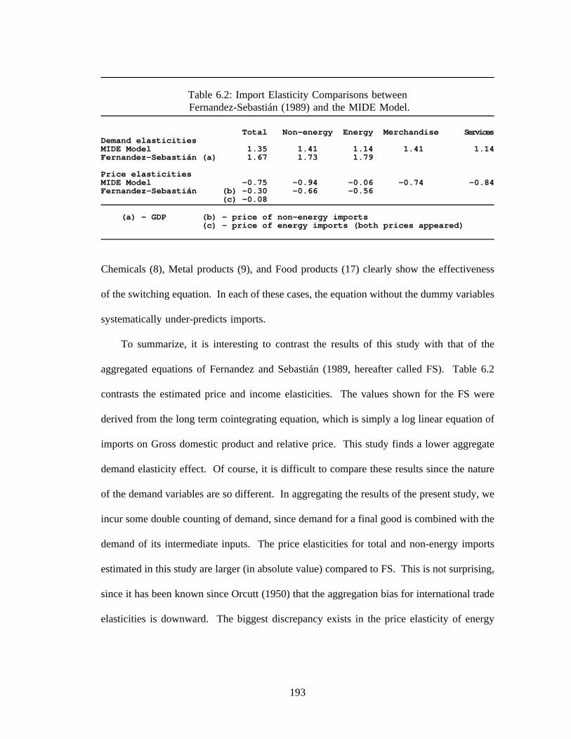
Table 6.2: Import Elasticity Comparisons betweenFernandez-Sebastián (1989) and the MIDE Model.
Total Non-energy Energy Merchandise ServicesDemand elasticitiesMIDE Model 1.35 1.41 1.14 1.41 1.14Fernandez-Sebastián (a) 1.67 1.73 1.79
Price elasticitiesMIDE Model -0.75 -0.94 -0.06 -0.74 -0.84Fernandez-Sebastián (b) -0.30 -0.66 -0.56
(c) -0.08
(a) - GDP (b) - price of non-energy imports(c) - price of energy imports (both prices appeared)
Chemicals (8), Metal products (9), and Food products (17) clearly show the effectiveness
of the switching equation. In each of these cases, the equation without the dummy variables
systematically under-predicts imports.
To summarize, it is interesting to contrast the results of this study with that of the
aggregated equations of Fernandez and Sebastián (1989, hereafter called FS). Table 6.2
contrasts the estimated price and income elasticities. The values shown for the FS were
derived from the long term cointegrating equation, which is simply a log linear equation of
imports on Gross domestic product and relative price. This study finds a lower aggregate
demand elasticity effect. Of course, it is difficult to compare these results since the nature
of the demand variables are so different. In aggregating the results of the present study, we
incur some double counting of demand, since demand for a final good is combined with the
demand of its intermediate inputs. The price elasticities for total and non-energy imports
estimated in this study are larger (in absolute value) compared to FS. This is not surprising,
since it has been known since Orcutt (1950) that the aggregation bias for international trade
elasticities is downward. The biggest discrepancy exists in the price elasticity of energy
193

imports. Where FS find a price elasticity of -.56 (only .1 below the non-energy elasticity),
this study computes it to be -.06.
This study also diverges in its findings concerning the structural implications of EC
integration. If we include Textiles and apparel and Wood products in the structural change
camp, but Metal products and Machinery (because of their simulation problems) in the no-
change camp, we find that 15 out of the 30 sectors for which equations were estimated
display structural change. However, if we weight the importance of these sectors according
to 1989 real imports, the proportion falls to only one third of the imports. If we exclude
energy imports (Sectors 2 through 4) from the calculation it rises again to 43 percent. FS
claim that the correct way to examine this situation is the dynamic structural approach where
the dependent variable, the change of imports, is regressed on the changes in short-term
variables and the errors given by the cointegrating equation mentioned above. However, the
most important short term effect in their analysis was the change of investment. Investment
goods tend to have large demand elasticities and account for a large proportion of total non-
energy imports (approximately 40 percent). Moreover, according to the results shown here,
import functions for the major equipment goods (Sectors 10-12) display stable behavior.
Therefore, it is possible that estimating equations that lump the equipment goods with all
other types of goods overestimates the structural stability of import behavior. It would be
interesting to adopt the FS approach to more disaggregated quantities (consumer,
intermediate and equipment goods, for example) and compare the results.
194

Merchandise Exports
The full functional form for merchandise exports (Sectors 1-25) is:
Xi,t (ai bi FDMi,t ci ∆DDi,t di DUMt )
2
k 0
(PXi,t k /FPEi,t k )
ηi
where: Xi,t = the exports of sector i in time t,
FDMi,t = an index of foreign demand,
∆DDi,t = the change in domestic demand,
DUMi,t = the dummy variable reflecting EC membership,
PXi,t = the export price at the border, and
FPEi,t = the foreign price of competing exports.
The foreign demand index, computed from the INFORUM international data base, is:
FDMi,tk
(wi,k,87 Mk,i,t / Mk,i,87 )
where: wi,k,87 = the share of Spanish exports for sector i which went tocountry k in 1987,
Mi,k,t = the imports for sector i and country k in year t.
As in any weighting scheme across time, the question of an appropriate base year muddles
the analysis. There is no doubt that the destinations for Spanish exports have changed and
will continue to change. Although it is near the end of the estimation period, the year 1987
was chosen because it is in the middle of the estimation-forecast period and reflects two
years of EC integration.
The change in domestic demand variable reflects that domestic demand pressures can
divert exports towards the domestic market. While capital utilization would be a better
variable to capture this effect, data is not available as this level of aggregation. It is
195

important in nine out of the twenty five industries. There is no particular pattern here, it is
significant in intermediate good sectors (4, 6, 7, and 8), equipment sectors (10 and 14) and
consumer good sectors (20, 22 and 23).
The foreign competing price of exports, calculated from the INFORUM international
base and model forecasts, are defined as:
FPEi,tk
(wi,k,85 pk,i,t rk,t )
where: wi,k,85 = country k’s share of world exports of commodity i in 1985,
pi,k,t = the domestic production price index (1980 = 1.0) for commodityi and country k in year t, and
rk,t = the exchange rate index (1980 = 1.0) of country k in yeart.
The model projects export prices with the percentage change in domestic prices. Table 6.3
shows the estimation results for the merchandise export equations.
Evidence of EC-induced structural change is not as clear here as with imports. Intercept
dummies starting after EC integration and varying in starting dates from 1986 through 1988,
are important in eight industries. In each case, the dummies enhanced the fit sufficiently
enough that full switching regressions were not necessary to obtain equations that performed
well in full model simulations. Apparently, exports of Agricultural (Sector 1), Meat (15)
and Dairy (16) products have benefitted from the Common Agricultural Policy (CAP) of the
EC. The Spanish government used to buy up the surpluses of these sectors. Some of the
surpluses, now purchased by the EC, are classified as exports. Exports of refined Petroleum
products (4) grew under integration as Spanish companies took advantage of the void left
by capacity reduction in the rest of Europe. Under a three year transition plan starting in
196

Table 6.3: Summary of Merchandise Export Regression Results.(t statistics in parenthesis.)
Sector Constant Demand Demand ∆Dom Dem Dummy Price Rbsq Rho 1989(a) (b) elast1 (c) (d) elas(η) weights exports
1 Agric., forest. -164.55 2.97 1.63 85.4352 -1.00 [.6 .4 .0] .94 .09 269.580& fisheries (-6.00) (10.14) ( 7.59)
2 Coal & radioact. 0.028 0.001 0.04 1.4893 -0.05 [.3 .5 .2] .95 -.45 1.291material ( 0.11) ( 0.21) (17.81)
3 Coke products -0.004 0.112 0.11 0.4302 -0.10 [.3 .5 .2] .51 -.23 0.644(-0.01) ( 0.20) ( 4.35)
4 Petroleum 102.070 2.347 0.82 -0.108 160.3492 -0.05 [.3 .5 .2] .95 .37 369.443products ( 1.10) ( 5.75) (-2.47) ( 9.03)
5 Electricity, 1.611 0.022 0.38 5.9255 -0.05 [.2 .2 .6] .60 .32 4.877gas & water ( 1.12) ( 1.26) ( 4.76)
6 Metal mining, -209.983 4.056 2.39 -0.312 -100.2712 -1.60 [.3 .5 .2] .67 .66 226.679processing (-2.17) ( 3.78) (-2.36) (-2.29)
7 Nonmetal mining -25.214 0.946 1.35 -0.199 -0.05 [.5 .3 .2] .86 .48 96.074and products (-2.45) ( 9.48) (-3.55)
8 Chemicals -112.790 2.300 1.57 -0.40 [.3 .5 .2] .95 .44 216.591(-8.90) (19.05)
9 Metal products -58.034 1.498 2.12 -0.022 -2.30 [.3 .5 .2] .87 .40 93.351(-6.73) (18.14) (-0.58)
10 Indust. & agric. -77.914 1.912 1.59 -0.031 -1.00 [.3 .5 .2] .97 -.01 169.020machinery (-10.16) (23.91) (-1.30)
11 Off. mach., -3.006 0.229 1.14 -0.15 [.3 .5 .2] .95 .30 54.162comput. & instr. (-1.74) (18.55)
12 Elect. & electron. -2.373 0.579 1.07 -0.45 [.3 .5 .2] .97 .41 94.199material (-0.99) (26.73)
13 Motor vehicles -126.257 2.698 1.60 -0.75 [.3 .5 .2] .96 .31 310.124(-10.28) (24.44)
14 Oth. transp. 50.037 0.005 0.01 -0.044 29.9684 -2.55 [.2 .5 .3] .72 -.05 53.809material ( 7.01) ( 0.10) (-1.61) ( 6.30)
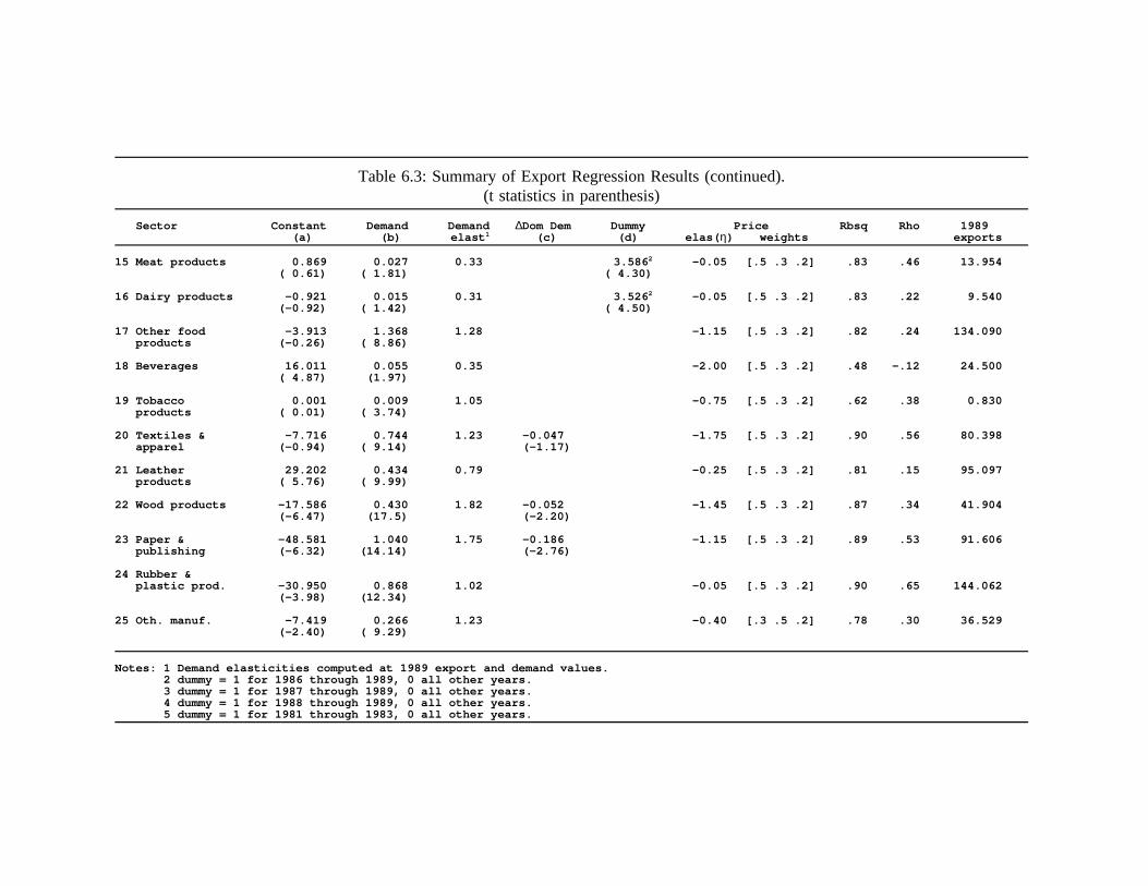
Table 6.3: Summary of Export Regression Results (continued).(t statistics in parenthesis)
Sector Constant Demand Demand ∆Dom Dem Dummy Price Rbsq Rho 1989(a) (b) elast1 (c) (d) elas(η) weights exports
15 Meat products 0.869 0.027 0.33 3.5862 -0.05 [.5 .3 .2] .83 .46 13.954( 0.61) ( 1.81) ( 4.30)
16 Dairy products -0.921 0.015 0.31 3.5262 -0.05 [.5 .3 .2] .83 .22 9.540(-0.92) ( 1.42) ( 4.50)
17 Other food -3.913 1.368 1.28 -1.15 [.5 .3 .2] .82 .24 134.090products (-0.26) ( 8.86)
18 Beverages 16.011 0.055 0.35 -2.00 [.5 .3 .2] .48 -.12 24.500( 4.87) (1.97)
19 Tobacco 0.001 0.009 1.05 -0.75 [.5 .3 .2] .62 .38 0.830products ( 0.01) ( 3.74)
20 Textiles & -7.716 0.744 1.23 -0.047 -1.75 [.5 .3 .2] .90 .56 80.398apparel (-0.94) ( 9.14) (-1.17)
21 Leather 29.202 0.434 0.79 -0.25 [.5 .3 .2] .81 .15 95.097products ( 5.76) ( 9.99)
22 Wood products -17.586 0.430 1.82 -0.052 -1.45 [.5 .3 .2] .87 .34 41.904(-6.47) (17.5) (-2.20)
23 Paper & -48.581 1.040 1.75 -0.186 -1.15 [.5 .3 .2] .89 .53 91.606publishing (-6.32) (14.14) (-2.76)
24 Rubber &plastic prod. -30.950 0.868 1.02 -0.05 [.5 .3 .2] .90 .65 144.062
(-3.98) (12.34)
25 Oth. manuf. -7.419 0.266 1.23 -0.40 [.3 .5 .2] .78 .30 36.529(-2.40) ( 9.29)
Notes: 1 Demand elasticities computed at 1989 export and demand values.2 dummy = 1 for 1986 through 1989, 0 all other years.3 dummy = 1 for 1987 through 1989, 0 all other years.4 dummy = 1 for 1988 through 1989, 0 all other years.5 dummy = 1 for 1981 through 1983, 0 all other years.

1986, Spanish government subsidies were progressively reduced to the iron and steel
industry (Metal mining and processing, 6). The reduction of subsides hurt exports to third
countries, and exports to the EC were still covered by (increasing) quotas (Salmon, 1991).
These factors account for the negative sign on the dummy parameter. Even though the
industry is now fully covered by the European Coal and Steel Community, the export
potential from the iron and steel industry is limited.
Curiously, the results displayed here seem to contradict the Fernandez and Sebastián
conclusion of a slight negative export impact of EC integration. Except for Metal mining
and processing (Sector 6) the seven dummies are positive. I suspect that the major reason
for the difference is that the disaggregated approach links exports with more precise
measures of foreign demand. The aggregate trade indices simply cannot capture the changes
in the components of demand. It is also true that the seven industries with positive dummies
account for only 26 percent of the total exports, so the aggregate effect of the dummies is
small. An aggregate equation could miss this effect.
Service Exports
Service exports in the MIDE model are treated differently than merchandise exports for
two reasons. First, since exports of Wholesale and retail trade (Sector 28) and the transport
sectors (30 through 32) consist mostly of margins earned by services rendered to
merchandise exports, they depend primarily on the volume of merchandise exports. Second,
price indices and world export shares for different countries are not available. Therefore,
it was not feasible to use relative price variables in the equations. In this event, the
nonlinear functional form is not applicable. Instead we utilize a simple linear function of
exports on the relevant demand variable. The equation results are displayed on Table 6.4.
199

Table 6.4: Summary of Service Export Regression Results(t statistics in parentheses)
Sector Constant Demand Demand Dummy Rbarsq Rho 1989elast1 exports
28 Retail & wholesale 8.229 0.059 1.01 .97 .68 153.055trade (-1.95) (22.76)
30 Highway & RR -0.631 .0115 0.71 13.2032 .99 .38 42.680transport (-0.74) (19.33) (12.26)
31 Air & water 82.909 0.062 0.66 .88 .39 245.682transport ( 9.56) (11.70)
32 Services assoc. 9.411 0.023 0.85 .88 .45 70.836with transport ( 2.90) (11.55)
33 Communications -36.476 0.458 3.38 .46 .61 16.150(-3.38) ( 4.13)
34 Banking & insur. -36.885 0.630 1.41 16.0192 .94 .46 53.409(-5.03) ( 8.07) (6.22)
35 Business serv. -79.857 1.193 2.60 .84 .40 54.629(-6.92) (10.06)
39 Other private 0.578 .061 0.93 .94 -.50 7.832services ( 0.47) (5.71)
Notes: 1 Demand elasticities computed at 1989 export and demand values.2 dummy = 1 for 1987 through 1989, 0 all other years.
For Wholesale and retail trade (28), Highway and rail transport (30), Air and water
transport (31), and Services associated with transport (32), the demand variable is
merchandise exports. An EC integration dummy is also highly significant for Highway and
rail transport. These equations explain the variables well. For the other sectors,
Communications (33), Banking and insurance (34), Business services (35) and Other private
services (39), external demand is represented by a variable which is simply a weighted (50-
50) index of the Gross domestic products of the United Kingdom and Federal Republic of
Germany. The variable is forecasted using the GDP projection taken from the German
model of the INFORUM international system. An EC integration dummy is used for
Banking and insurance. The fits for each of these sectors, except for Communications, are
very good.
200

Table 6.5: Export Elasticity Comparisons betweenFernandez-Sebastián (1989) and the MIDE Model.
Total Non-energy Energy Merchandise Services
Demand elasticitiesMIDE Model 1.33 1.39 0.82 1.40 1.07Fernandez-Sebastián (a) 1.78
Price elasticitiesMIDE Model (b) -0.80 -0.92 -0.05Fernandez-Sebastián (c) -0.87
(a) - world trade index (c) - domestic vs. world price index(b) - merchandise exports only
Table 6.5 displays aggregate elasticities for the results given here, again using 1989
weights. While recognizing that the nature of the respective demand variables are very
different, I include results for one of the Fernandez and Sebastián aggregate export
equations. They estimated five equations, each corresponding to different combinations of
international trade and price indices (world, industrialized countries and EC countries). For
the comparison, I chose the equation using the world trade and price indices. Notably, the
weighted MIDE model total price elasticity (-.80) is lower than the FS result. If energy
exports (mostly refined petroleum products) is taken out, it rises to -.924.
Tourism Imports and Exports
The MIDE model equation for real, per capita Exterior consumption by Spanish
residents (tourism imports) is specified in first differences. It does not have an intercept.
The explanatory variables are the current and lagged differences in real per capita household
disposable income, the difference in the moving average of the relative price, and a dummy
from 1974 through 1976. The relative price is the price index for the dependent variable
from the national accounts divided by the price index for Private interior consumption. The
201

moving average weights are .3 in the current year, .5 for the last year, and .2 for two years
ago. The MIDE model projects the price index of tourism imports with a simple regression
equation using a two period weighted average of the exchange-rate-adjusted German and UK
consumption deflators. The deflator is forecasted with the German consumption deflator
from the INFORUM system German model. The dummy variable reflects the oil crisis and
the political turmoil surrounding Franco’s death. The combination of these events generated
a decline in the outflow of tourists. The equation results, statistics and regression plot for
are shown in the top half of Figure 6.3. A second graph displays the estimation in the level
of Exterior consumption using the actual lagged value of the dependent variable as the base
for computing the current predicted value.
The tourism export equation is similar to the import equation. The first difference of
the variable depends on a constant, the first difference of a demand index and the first
difference of a two-period moving average relative price. The weights on the moving
average are .4 for the current year and .6 for the previous year. Spanish tourism exports
depend to a large extent on the inflow of German and British tourists. While the numbers
of French and Portuguese visitors is larger, most of these make only day trips. The
Germans and British tend to fly in to the holiday resorts and stay for a week or more. The
demand variable for tourism exports, therefore, is the weighted index between the UK and
German GDP (the same variable used for the service export equations). The denominator
of the relative price is the same variable which projects the tourism import price (combined
German-UK consumption price deflator). The bottom half of Figure 6.3 displays the
regression results. While the general results are disappointing, the equation did capture the
sharp decline in 1989 and 1990. The striking result from both equations, especially the
export equation, is the powerful influence exerted by the relative price variables.
202

Figure 6.3: Estimation Results for Imports and Exports of Tourism, 1971-90
Exterior consumption by Spanish residents (imports)
Predicted vs. actual in first differences Predicted vs. actual in levels
SEE = 0.21 RSQ = 0.5356 RHO = 0.25 Obser = 20 from 1971SEE+1 = 0.21 RBSQ = 0.4485 DW = 1.50 DoFree = 16 to 1990MAPE = 1016.25
Variable name Reg-Coef Mexval t-value Elas Mean0 dimptourpc - - - - - - - - - - - - - - - - - - 0.211 dYpc 0.0096 3.2 1.026 0.28 6.162 dYpc(t-1) 0.0118 3.0 0.992 0.32 5.663 dmarelprice -4.5799 23.2 -2.878 0.44 -0.024 dum74-76 -0.4132 33.0 -3.507 -0.39 0.20
Domestic consumption by non-residents (exports)
Predicted vs. actual in first differences Predicted vs. actual in levels
SEE = 41.96 RSQ = 0.3558 RHO = 0.06 Obser = 20 from 1971SEE+1 = 41.91 RBSQ = 0.2800 DW = 1.89 DoFree = 17 to 1990MAPE = 136.40
Variable name Reg-Coef Mexval t-value Elas Mean0 dexptour - - - - - - - - - - - - - - - - - - 10.631 intercept 54.2929 18.2 2.600 5.11 1.002 ddem (UK&Germ) 2.0288 0.3 0.340 0.46 2.403 dmarelprice -9.9750 23.9 -3.015 -4.57 4.87
203
6.2 Productivity and Employment
Productivity growth is a crucial issue in any discussion of economic development and
policy. The productivity level determines the competitive standing of and the relative level
of living standards in an economy. Paul Krugman (1990) expressed this fact by saying,
"Productivity isn’t everything, but in the long run it is almost everything" (p.9). Economists
have long conceded that it is difficult to quantify the underlying factors contributing to
productivity growth. Solow’s famous empirical results on the origins of growth estimated
that technical progress, an admittedly ambiguous concept, accounted for about half of the
growth in per capita output. It is clear that growth is the result of many interrelated factors
such as age, composition and expansion of the capital stock; the educational level,
experience and abilities of the labor force; research and development efforts; and the
exploitation of economies of scale. The output composition of an economy also influences
productivity growth. Some industries display consistently healthy productivity growth;
others, consistently slow growth; and still others, quite variable growth. Therefore, an
interindustry modeling approach provides a particularly convenient framework for examining
the questions surrounding the course of productivity performance.
Sectoral labor productivity in the MIDE model is a simple variable: constant-price
output divided by the total hours worked by all workers, including the self-employed. This
concept is different from total factor productivity which is net of increased output
contributed by additional capital and intermediate goods, as well as additional labor inputs.
Total factor productivity growth is a more appropriate measure of the additional output
resulting from technical progress, economies of scale, increased know-how, and other
factors. However, since the primary role of productivity in the MIDE model is to determine
the amount of employment in each industry, labor productivity is the variable modeled.
204

After generating estimates for sectoral labor productivity, the MIDE model computes
sectoral employment in hours worked by dividing output by the productivity estimate. The
model also contains sectoral equations to estimate the average annual hours worked per
worker. Dividing this figure into the total hours worked in the industry provides the total
jobs in each industry. Sectoral employment affects the computation of wages. If labor
productivity in a certain sector increases at a rate high enough to decrease the unit labor
costs in that sector, the relative price of its product will fall and, demand for the product will
increase. Moreover, total employment (via the unemployment rate) enters into the aggregate
wage index equation. In this equation, productivity growth decreases wage pressure because
it reduces labor requirements. This reduction in inflationary pressures increases real income
and aggregate demand, allowing for faster growth in the economy as a whole. Therefore,
as in the real economy, productivity plays a key role for determining real economic growth
in the model. Before discussing the sectoral level behavioral of productivity, however, some
remarks on aggregate labor productivity are in order.
Since 1960, average annual labor productivity growth (measured as GDP over
employment) in Spain has been substantially higher than in the rest of the OECD (Larre and
Torres, 1991). This tendency is consistent with theoretical expectations. Neoclassical
growth models conclude that a nation starting from lower levels of productivity will catch-up
to the levels of more advanced nations. Lower relative levels of labor productivity imply
a higher return on capital, which will induce flows of labor-augmenting capital investment
from more productive countries. Moreover, this investment normally embodies more
advanced technology than that already existing in the country. The upshot of this theory is
that convergence in living standards (real convergence as defined in Chapter 2) between less
developed and developed countries is a spontaneous process. However, various institutional
205
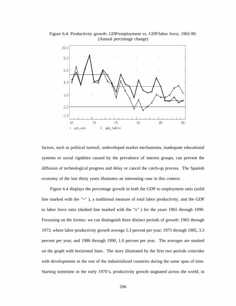
Figure 6.4: Productivity growth: GDP/employment vs. GDP/labor force, 1965-90.(Annual percentage change)
factors, such as political turmoil, undeveloped market mechanisms, inadequate educational
systems or social rigidities caused by the prevalence of interest groups, can prevent the
diffusion of technological progress and delay or cancel the catch-up process. The Spanish
economy of the last thirty years illustrates an interesting case in this context.
Figure 6.4 displays the percentage growth in both the GDP to employment ratio (solid
line marked with the "+" ), a traditional measure of total labor productivity, and the GDP
to labor force ratio (dashed line marked with the "x" ) for the years 1965 through 1990.
Focussing on the former, we can distinguish three distinct periods of growth: 1965 through
1973, where labor productivity growth average 5.3 percent per year; 1975 through 1985, 3.3
percent per year; and 1986 through 1990, 1.0 percent per year. The averages are marked
on the graph with horizontal lines. The story illustrated by the first two periods coincides
with developments in the rest of the industrialized countries during the same span of time.
Starting sometime in the early 1970’s, productivity growth stagnated across the world, in
206

contrast to the very high rates of growth displayed from 1945. Spain was not immune to
this phenomena. As explained in Chapter 2, various international economic and domestic
political circumstances contributed to a general stagnation of the economy from 1975
through 85. What is curious about Spain, however, is the significant fall in productivity
growth which started in 1986 (Figure 6.4). This decline started at the very time that the
economy began to expand.
Another description of the story is given by the second line of Figure 6.4, which depicts
the growth in the GDP to labor force ratio. It illustrates that the productivity problem of the
economic crisis, especially from 1977, was much worse if we consider the utilization of
labor. The difference between the two lines suggests that the economy maintained labor
productivity growth precisely because employment fell. Explanations for this phenomena
are many and complex. It is evident, however, that stagnation of demand led to the idling
of the least efficient plant and equipment. The accompanying job losses, therefore, were of
relatively less productive positions. Moreover, the political climate, large rates of inflation,
and the rigid regulation of the labor market created an unfavorable environment for the
formation of employment. Various studies conclude that throughout the 1970’s, productive
investment tended to favor capital intensive techniques because of the accelerating real costs
of labor and the high fixed costs of hiring (Ballabriga et al. 1990; Malo de Molina 1990).
Moderation of labor cost growth in the early 1980’s did not change the story because capital
formation was anemic, and government sponsored restructuring gave over-staffed industries
the opportunity to increase productivity by releasing workers.
Continuing labor market reforms initiated by the Moncloa Pacts of 1977 and the
Estatuto de los Trabajadores (Worker’s Statute) of 1980 have gradually decreased the
rigidities in the labor market. Probably the most significant aspect of this reform was the
207

introduction of fixed-term employment contracts as opposed to the permanent employment
contracts. The existence of these contracts opened the door for part-time work and
employment-training programs, which were previously nonexistent. These arrangements
increase the flexibility of the labor market and reduce the fixed costs of hiring. Although
they apply to new jobs only, by 1990 almost thirty percent of new jobs were covered under
these contracts (Jimeno and Meixide 1991). More competition and flexibility in the labor
markets suppresses excess wage growth and encourages capital formation in line with the
relative factor endowments. Therefore, when economic growth started to pick up in 1986,
the growth of aggregate labor productivity, paradoxically, fell dramatically. Rather than
being a negative development, the employment creation and renewed growth of labor force
productivity shows that the economy is providing a more favorable environment for the
increase in living standards. On the other hand, one percent growth of labor productivity
is certainly not a figure which encourages contentment. The hopeful expectation is that once
the labor market tightens, firms will again find it profitable to invest in labor-saving
production techniques that will again boost Spanish productivity growth above the developed
world average.
Labor Productivity
All previous examinations of industrial level productivity for the Spanish economy used
either annual output, or more commonly value added, divided by annual employment
(number of workers) as the measure of labor productivity (see, for example, Segura et al.
1989, Martín Marcos 1990 and Treadway 1990a). This is the most convenient method since
reliable employment data is available from the Encuesta Población Activa (Labor Force
Survey) of the Instituto Nacional de Estadística (INE). However, employment is an
208

inaccurate measure of labor input because annual hours per worker tend to fluctuate from
year to year. More important, hours per worker year have displayed a strong tendency to
decrease over time. Because of this tendency, previous studies have underestimated labor
productivity growth.
This work attempts to measure and analyze productivity growth in terms of output per
hours worked. The sectoral hours worked figures are acquired by multiplying employment
by the annual hours worked by employee. The endeavor is complicated by the lack of
disaggregated data on hours. The Encuesta de Salarios (Wage Survey) of the INE is the
best source of such data. It publishes a quarterly figure of the average monthly hours
worked for that quarter. In 1989, the Wage Survey began to publish hours worked data at
a sufficient disaggregation for MIDE’s sectoral scheme. Previous to then, published data
enumerated only 17 sectors. The collection of the data suffered several methodological
breaks, which made it difficult to compare data from different periods. However, Carbajo
and Perea (1987) homogenized the series to provide continuous time series from 1963 for
each of the 17 sectors. In order to reach hours worked per year for each of the MIDE
sectors, I assumed that the annualized Carbajo and Perea data is the same for the MIDE
sectors covered by a single Wage Survey sector. For example, the Wage Survey published
one figure for the food processing, beverage and tobacco industries. Therefore, the
corresponding MIDE sectors (15-19) have identical series for annual hours worked per
worker.
This assumption probably distorts productivity estimates for individual sectors over
production cycles. However, it goes a long way towards reducing the downward bias in
productivity growth produced by using output over employment productivity measures. If
the downward trend in annual hours worked per worker were a simple linear function, the
209

productivity bias would not have was serious consequences for employment projections.
This is because the effect of the work-year trend would be captured by the time-trend
variable in the equation explaining productivity growth. As explained below, however, the
downward trend in annual hours has recently been moderating. Therefore, if the MIDE
model does not explicitly consider the non-linearities in the trend, productivity projections
assuming a linear inclination of hours worked would overstate growth. Over a long period,
this would have serious repercussions for the computation of employment.
Theoretical approaches for determining labor required per unit of output use various
production functions which include other factors of production, especially the capital stock,
to estimate own and cross-price elasticities of demand for labor. Therefore, labor
productivity becomes a function of all the factor prices. Unfortunately, the lack of industry
level capital stock data for the Spanish economy prevents me from taking such approach.
At any rate, when production-function-based labor demand equations are used in
multisectoral models, a time trend term is inevitably included in order to account for
technical progress. Often, the time trend becomes the overriding explanatory variable and
the price elasticity terms are insignificant (Almon, et.al. 1974, pp.173-177). Other
INFORUM models have normally modeled labor productivity specification as a simple
function of time and output (see, for example, Werling 1989). While lacking in
microeconomic theoretical content, the approach is simple, easy to implement, and provides
well behaved and accurate employment predictions. This approach is used here.
The logarithm of labor productivity is projected using regression equations which
include time and two output fluctuations as independent variables. The labor market
upheaval which occurred during the estimation period makes any estimation of sectoral level
productivity trends a difficult endeavor. Sectoral productivity trends have tended to follow
210

a pattern similar to aggregate productivity. Growth in the late 70’s and early 80’s was very
high, but started to rise at a declining rate in the mid-80’s. In manufacturing, employment
reduction effects of reconversion programs (most were completed or almost completed by
1986) have inflated productivity growth trends. For all the sectors, changes in wage-setting
behavior since the 1977 and labor market reforms (see Chapters 2 and 7) have increased the
attractiveness of labor relative to capital. Therefore, much of the recent investment has been
capital augmenting, rather than labor augmenting. To capture this recent slowdown in
productivity growth, the equations include a second time trend.
The output variables (QDN and QUP, below) are designed to capture the behavior of
productivity over the business cycle. The source of cyclical fluctuations is straightforward.
In the downward part of the cycle firms tend to keep standard hours and retain skilled
workers on the payroll (i.e., labor hoarding), despite falling levels of output. In an upswing,
output tends to rise faster than hours worked and new hiring. Therefore, productivity
increases during an expansion and falls during a contraction. The equation includes two
variables in order to estimate the asymmetrical nature of the productivity fluctuations. These
variables are formed by subtracting the previous peak level of output, representing potential
output, from the current period output. If this difference is positive, meaning that the
industry is in an upswing, it becomes the QUP variable and QDN is zero. A negative
difference, indicating that the industry is in recession, becomes the QDN variable and QUP
is zero. Given the differing signs on QUP and QDN, both the d and e coefficients are
expected to be positive. They also must be less than one. A coefficient greater than one
would predict declining employment for production increases or increasing employment with
production decreases.
Each industry equation is of the form:
211

ln(Qi,t / Hi,t) = ai + biT1t + ciT2t + diQDNi,t + eiQUPi,t
where: Qi,t = output of sector i in period t,
Hi,t = total hours worked,
T1t = a time trend covering the entire estimation period,
T2t = a time trend beginning in 1986,
QDNi,t = lnQi,t - lnQPKi,t-1 when QPKi,t-1 > Qi,t
= 0 when QPKi,t-1 < Qi,t,
QUPi,t = lnQi,t - lnQPKi,t-1 when QPKi,t-1 < Qi,t
= 0 when QPKi,t-1 > Qi,t,
QPKi,t = Qi,t when Qi,t > QPKi,t-1 * (1 - si)
= QPKi,t-1 * (1 - si) when Qi,t < QPKi,t-1 (1 - si).
The equations are fit for the period 1972 through 1989, except for sectors 36 through 43.
For these service sectors, employment data is adequate for equations only from 1976 through
1989. Table 6.6 displays the estimated equation parameters, autocorrelation coefficients and
adjusted R-squares of the regressions. Parameter significance statistics are not displayed,
since the rather heavy use of soft constraints (explained below) renders them meaningless.
There is ample evidence of productivity growth slowdowns in most of the industries.
For some sectors, it is also apparent that the slowdown began before 1986. Rather than
embarking on a laborious, and somewhat arbitrary, search for the best breaking point, the
second trend begins in 1986, except in one instance. For Communications (Sector 33), the
second time trend starts in 1980 where a clear and strong change in the productivity trend
occurred. In other sectors, the second time trend adds nothing to the fit of the equation, and,
212

therefore, is not included (signified by a blank line under in the c column of Table 6.6).
Given the logarithmic structure of the equation, the sum of the two time trend coefficients
(b and c) is the exogenous rate of productivity growth used in the MIDE model. The total
trend, in percent, is displayed in the fourth column of Table 6.6. Soft constraints are used
where they conserve sensibility in the estimated trends. In every case, these constraints do
little harm to the fit of the equation.
Differences between the d and e parameters of Table 6.6 indicate that asymmetry
between the different stages of the business cycle does indeed exist. Unfortunately, for the
estimation period of 1972-89, many sectors of the Spanish economy displayed a-cyclical
productivity growth. As explained, the scrapping of older and inefficient plant during
industrial reconversion led to productivity increases at the same time of production declines.
However, the ultimate use of the equations will be for forecasting, when the economy,
hopefully, will be experiencing less upheaval. It is reasonable to assume that future
productivity growth will respond pro-cyclically to output fluctuations, and it is therefore
important to integrate this property into the equations. One way of dealing with this
problem is to decrease the peak, or potential output, of a restructuring sector by a constant
proportion, shown above as the parameter si, each year. Industry equations using a non-zero
si are noted in Table 6.6. Where this technique does not work (i.e., when unconstrained
coefficients are negative or greater than one), soft constraints are used.
Electricity generation (Sector 5) and several service sectors (29, 36, 41-43) experienced
stable output increases throughout the estimation period. Therefore, output fluctuation
variables add nothing to the equation and are not included. Business services (Sector 35)
is the only sector which displays a pervasive downward trend in productivity. While
productivity growth in this sector is undoubtably slow, the problem lies with an unreliable
213

Table 6.6: Summary of Labor Productivity Equation Results
sector const time1 time2 trend qup qdown rho rbsq(a) (b) (c) (%) (d) (e)
1. Agric, f & f2. Coal3. Coke4. Petroleum5. Electricity
6. Met mng, proc7. Nmet mng, proc8. Chemicals9. Met prod
10. Ind mach
11. Off mach12. Elect prod13. Motor veh14. Oth tran eq15. Meat prod
16. Dairy prod17. Oth food18. Beverages19. Tobacco20. Text & app
21. Leather prod22. Wood prod23. Pap & publ24. Rub & plas25. Oth mfg prod
26. Construction27. Rep & reconst28. Trade29. Rest & hotels30. Int transport
31. Marit & air32. Transp serv33. Communic34. Bank & insur35. Bus serv
36. Rents37. Priv educ38. Priv health39. Oth serv40. Publ Adm
41. Publ educ42. Publ health43. Dom serv
-1.80 0.086 -0.026 6.06 0.142 0.053 .70 .99-0.65 0.098 -0.053 4.50 0.497 0.504 .78 .922.21 0.042 4.18 0.849 0.496 .24 .913.41 0.036 3.64 0.580 0.594 .31 .830.99 0.049 -0.017 3.18 .34 .94
1.31 0.061 -0.019 4.20 0.366 0.443 .49 .920.10 0.038 -0.018 1.93 0.300 0.278 .31 .950.34 0.063 -0.030 3.31 0.478 0.513 .07 .980.04 0.024 -0.013 1.12 0.095 0.100 .18 .790.36 0.038 -0.019 1.93 0.267 0.204 .47 .82
0.14 0.095 -0.037 5.75 0.526 0.592 .32 .910.05 0.057 -0.018 3.83 0.695 0.542 .47 .930.56 0.054 -0.010 4.41 0.299 0.731 .21 .970.46 0.020 2.00 0.621 0.841 .47 .941.60 0.024 -0.013 1.12 0.230 0.262 .63 .86
1.22 0.023 -0.009 1.39 0.445 0.595 .49 .900.14 0.072 -0.033 3.95 0.415 0.505 .75 .960.19 0.070 -0.045 2.55 0.554 0.497 .78 .960.95 0.056 -0.029 2.71 0.740 0.572 .61 .95
-0.38 0.032 -0.015 1.69 0.391 0.301 .53 .90
-0.60 0.063 -0.036 2.73 0.567 0.592 .69 .90-0.48 0.027 -0.014 1.29 0.417 0.434 .74 .67-0.20 0.069 -0.059 1.04 0.593 0.096 .47 .930.09 0.050 -0.003 4.70 0.722 0.799 .49 .94
-0.97 0.109 -0.064 4.48 0.381 0.520 .59 .93
-0.19 0.040 -0.024 1.65 0.428 0.347 .18 .98-0.31 0.033 3.32 0.656 0.511 .58 .87-0.57 0.030 -0.013 1.70 0.151 0.479 .77 .920.07 0.032 -0.025 0.70 .57 .96
-0.65 0.054 -0.024 3.00 0.499 0.497 .32 .98
0.31 0.062 -0.014 4.82 0.362 0.502 .20 .970.05 0.025 2.45 0.527 0.500 .54 .64
-1.09 0.155 -0.112* 4.00 .23 .990.37 0.044 -0.022 2.23 0.563 0.496 .68 .940.52 0.020 -0.171 -15.11 0.987 -4.076 .32 .81
4.12 0.160 -0.089 7.10 .34 .75-0.51 0.007 0.67 0.400 0.396 .11 .43-0.39 0.029 -0.002 2.64 0.563 0.458 .36 .80-0.39 0.016 -0.011 0.57 0.414 0.515 .32 .640.80 0.001 0.12 .24 -.05
-0.53 0.008 0.83 .21 .57-0.40 0.030 2.99 .41 .84-1.72 0.006 0.63 -.34 .62
* - time2 begins in 1980.
Sectors where si > 0: i = 3 si = .025 i = 20 si = .05(see text) i = 7 si = .03 i = 21 si = .05
i = 9 si = .05 i = 22 si = .05i = 10 si = .05 i = 26 si = .05i = 12 si = .02 i = 37 si = .01i = 14 si = .03 i = 38 si = .01
214

output series. Continually decreasing productivity leads to a rapidly increasing and
unreasonable employment forecast. In the MIDE model, therefore, the projections assume
constant productivity equal the 1989 level. For Public administration (sector 40) hours
worked are not published. Output over employment for the sector displays no underlying
trend, and in fact has been stationary for many years. Therefore, employment in the sector
is determined by multiplying the historic mean of the output to employment ratio by
output.9
Annual Hours Worked per Employee
As in most nations, the number of hours in the average work-year for Spanish workers
fell dramatically through the past thirty years. In the period from 1976 to 1989, the average
hours worked per year declined from 2244 to 1835, a fall of over 18 percent. One way,
then, to project the work year is to use a simple linear time trend. A measure of output
fluctuation can be included in the specification to account for work-year fluctuations due to
overtime in periods of high production and short-time in periods of low production.
However, the strong downward tendency of the work-year has begun to moderate over
the past several years. There are reasons to expect this moderation to continue. Large
expansions in participation by female workers and the coming of age of Spain’s baby boom
have just about been played out. Therefore, labor force growth is expected to slow for the
rest of this century and beyond. The tighter labor market will prevent further reductions in
the work week. Furthermore, the number of Spanish holidays and length of vacations
already meet or exceed the standards in other EC countries. While expansion in the use of
9 Note that since the output of public administration is exogenous governmentconsumption, this method for determining government employment is equivalent tospecifying it exogenously.
215

part-time labor may act to reduce the work week of the average worker, extrapolating the
trends over the past two decades leads to 25-30 hour work weeks in several sectors. This
is an implausible result.
The problem is handled by projecting the average work year using an exponential trend.
This trend adequately captures the recent deceleration in the tendency of the work-year. It
allows for further decreases in the work year by the year 2000, but at a much more
reasonable rate. The forecast equations are of the form:
lnHYRi,t = ai + biTRENDi,t + ciDOUTi,t
where: HYRi,t = average annual hours per worker in sector i at time t,
TRENDi,t =
1 exptime× ln(1 si)
si
DOUTi,t = the first difference of the log of output.
The trend variable is an increasing function of time, and, therefore, the bi parameter is
negative. The higher the si parameter, the greater is the deceleration in the decrease of the
work-year. The si is chosen with a subjective iterative procedure based on which parameter
provides the best fit and a reasonable work year by the year 2000, given a change in output
of zero. Most of the sectors reach 1600 to 1700 hours per year. These figures correspond
to a 35 to 37 hour work week for a 46 week work year (52 weeks minus 4 weeks vacation
and 2 weeks of holidays). For several service sectors, the si is considerably low. The low
value results because increased use of part time labor in the sectors produces only a small
deceleration of the downward trend. The equation includes the change in output variable
to explain cyclical changes in the average work-year. It is not used for equations where
216

the estimated parameter is negative or in those for which output has never, or rarely,
declined in the estimation period (1975 through 1989).
Table 6.7 summarizes the estimation results. The si parameter is displayed in the first
column. A close examination of the table reveals that several sectors have identical or
nearly identical parameter estimates (sectors 31 and 32 for example). This is because they
are the same data series under our adaptation of the wage survey data. (Slight differences
arise because the 1989 figure may be different because they are linked on to the previous
series using the revised, more disaggregated, wage survey.) Figure 6.5 provides graphs
showing examples of fits and forecasts for six of the most important sectors (by share of
employment). The lines with the "+" are predicted values; those with the " " are actual
values. The projections through the year 2000 assume that the change in output is zero.
The plots clearly show the desirability of using the exponential approach both for estimation
and forecasting purposes.
217

Table 6.7: Summary of Hours per Worker-year Equations.
sector s const trend dq rho rbsq(a) (b) (c)
1. Agric, f & f2. Coal3. Coke4. Petroleum5. Electricity
6. Met mng, proc7. Nmet mng, proc8. Chemicals9. Met prod
10. Ind mach
11. Off mach12. Elect prod13. Motor veh14. Oth tran eq15. Meat prod
16. Dairy prod17. Oth food18. Beverages19. Tobacco20. Text & app
21. Leather prod22. Wood prod23. Pap & publ24. Rub & plas25. Oth mfg prod
26. Construction27. Rep & reconst28. Trade29. Rest & hotels30. Int transport
31. Marit & air32. Transp serv33. Communic34. Bank & insur35. Bus serv
36. Rent37. Priv educ38. Priv health39. Oth serv
41. Publ educ42. Publ health43. Dom serv
0.08 1.941 -0.107 0.082 .38 .980.03 0.487 -0.002 0.454 .13 .830.10 1.940 -0.158 0.059 .38 .880.08 1.781 -0.112 0.096 .39 .930.12 1.889 -0.164 0.077 .38 .96
0.10 1.719 -0.122 0.041 .03 .970.08 1.596 -0.089 .52 .960.09 1.713 -0.109 .12 .950.08 1.752 -0.105 0.150 .14 .930.09 1.911 -0.130 0.064 .15 .91
0.10 2.014 -0.151 .43 .930.09 1.820 -0.120 0.007 .42 .930.10 1.348 -0.082 0.021 .41 .780.10 1.385 -0.086 0.026 .49 .790.10 2.228 -0.173 0.265 -.19 .99
0.10 2.205 -0.170 0.094 .12 .980.10 2.191 -0.168 0.058 .12 .980.10 2.200 -0.169 0.005 .19 .970.10 2.195 -0.169 0.074 .39 .980.08 1.640 -0.094 .44 .93
0.10 2.109 -0.161 -.01 .920.06 1.414 -0.059 0.085 .51 .830.06 1.289 -0.052 0.053 .04 .950.06 1.300 -0.053 0.051 .43 .890.05 1.215 -0.042 .46 .90
0.08 1.720 -0.100 0.171 .37 .920.03 1.138 -0.027 .39 .970.03 1.140 -0.027 .36 .980.05 1.211 -0.036 .46 .980.03 1.134 -0.026 .35 .97
0.03 1.134 -0.026 .35 .970.03 1.136 -0.026 .33 .970.03 1.140 -0.027 .36 .980.05 0.936 -0.022 -.44 .970.10 1.262 -0.071 .19 .89
0.10 1.262 -0.071 .19 .890.03 0.870 -0.014 -.44 .950.03 1.140 -0.027 .36 .980.03 1.138 -0.027 .39 .97
0.03 0.870 -0.014 -.44 .950.03 1.140 -0.027 .36 .980.03 0.870 -0.014 -.44 .95
218

Figure 6.5: Regression Fits for Hours per Worker-year Equations.
Sector 1: Agriculture, forest & fish., s = .08 Sector 9: Metal products, s = .08
Sector 17: Other food products, s = .10 Sector 26: Construction, s = .08
Sector 28: Wholesale & retail trade, s = .03 Sector 35: Business services, s = .10
219

CHAPTER 7:
EQUATION SPECIFICATION AND ESTIMATION:
EMPLOYMENT AND CAPITAL INCOME
This chapter describes the determination of sectoral level, nominal labor and capital
income of the MIDE model. The sum of this income, together with net indirect, import and
value added taxes, yields the Gross Domestic Product in current prices. Moreover, sectoral
labor and capital income are leading determinants of production prices.
Several different approaches have been used to determine industry level prices and
incomes in macroeconomic multisectoral models. For example, the Cambridge multisectoral
model (CMDM) of the United Kingdom projects industry wages, net taxes and price indices
using behavioral functions. Once these quantities are determined, capital income (profits,
capital consumption, interest) can then be computed using the input-output price equation,
solved for the capital portion of value added (see Barker and Williamson 1987). The
INFORUM group of models, however, predict each component of value added and then
solve for industry prices using the input-output price equation in its familiar form (see
Chapter 4). With this scheme, value added equations, especially gross profit equations,
include many variables often found in price functions, such as changes in output or capital
utilization. In comparison to models of other nations, the price-income block of MIDE is
relatively simple. This simplicity was mandated by data constraints.
At the outset of this project, lack of data introduced serious problems for specification
and estimation of the value added equations of the MIDE model. The 1980 Spanish input-
output table distinguishes six types of value added for each sector: wages and salaries, social
security taxes, capital income, indirect taxes and subsidies. However, the national accounts
220

provide time series data for only three types of value added: gross wages (including social
security taxes), capital income, and net indirect taxes (taxes minus subsidies). While
attempts could be made to divide gross wages and net taxes over time, such procedures
would necessitate an allocation which assumes that the proportion of each component, per
sector, changed at the same rate as the aggregate (macroeconomic) component proportion.
There is no reason to believe, especially in the case of taxes and subsidies, that this is a
valid assumption. Therefore, the combined series for wages and net taxes, as published, are
used in the MIDE model.
A second problem was that the value added series for wages and profits started only in
1980. The previous version of the national accounts (Base 1970) published the sum of
wages and profits (value added at factor cost) and the total value added (value added at
market prices) for each sector. More importantly, this data was at a substantially different
aggregation than the 1980 table (Sanz 1989). Several attempts were made to homogenize
the sectoral data at the level of value added at factor cost. However, complications due to
overlapping sectoral definitions between the two versions of the national accounts could not
be solved. The resulting series displayed peculiar behavior which led to serious problems
for estimation. This approach was abandoned. Therefore, the available data for equation
estimations spans the short period of 1980 through 1987, and the specifications are severely
constrained by the lack of observations. Particularly, it is difficult to include the lagged
effects of explanatory variables under this constraint. Distributed lags, for example, entail
lost degrees of freedom. The profit equations cannot include the past values of labor costs
because this also entails a reduction of equation observations.
Because of these problems, I have taken an approach designed to capture the most
important influences on wages, profits and prices in the Spanish economy, while leaving
221

other factors aside. For example, wage bargains between industry and labor in Spain are
relatively centralized. Therefore, a simple Phillips curve equation for aggregate wages does
much of the work to determine sectoral wages. With the opening of the Spanish economy
to international trade, domestic price setting has become much more responsive to foreign
competition. In the MIDE model, profit margins for tradeable goods depend to a large
extent on the international prices of the goods. Despite the parsimonious nature of the price-
income block of MIDE, it successfully accounts for the crucial determinants of prices in the
economy.
7.1 Employment Income
Before elaborating on the aggregate and industry wage functions, a brief comment
covering wage setting institutions of the Spanish economy is in order. Under the Franco
dictatorship, wages and working conditions were set by a process of collective bargaining
dominated by government intervention (Toharia 1988; Jimeno and Meixide 1991).
Officially, all employees were part of vertical unions comprising both labor and
management. Even though unemployment was very low, real wage increases during this
period tended to follow the growth of labor productivity. This system broke down in the
early 1970’s with the political turmoil surrounding the illness and death of Franco and the
economic crisis following the oil price increase of 1973. Because of political upheaval, the
monetary authorities attempted to avoid the real adjustments made necessary by the oil price
shock and accommodated the ensuing inflation. Workers were able to demand, and receive,
their traditional increases in real wages. However, since the oil price shock adversely
effected productivity, the wage increases led to excess demand and more inflation.
222

As noted in Chapter 2, this inflationary spiral led to a severe crisis by 1977. Inflation
was at an all time high, while GDP and employment growth were stagnant. The current
account balance was in serious disequilibrium. The Moncloa Pacts of that year initiated a
more tranquil transition to democracy which, among other things, resulted in a tremendous
change in the system of labor relations. One major and immediate outcome of the Moncloa
accord was the inclusion of wage setting guidelines intended to break with the tradition of
full wage indexation. According to these guidelines, nominal wages should be increased
along a forecasted (or expected) inflation rate set by the government. In 1978, nominal
wage growth dropped sharply, a trend that continued for several years (Figure 7.1). By
1979, real wage growth was below average labor productivity growth, a feature which
continued throughout the 1980’s.
Currently, the main process for the determination of wages and employment conditions
is collective bargaining. This dialogue is relatively centralized and takes place between
representatives of the two major unions, the socialist Unión General de Trabajadores (UGT)
and the Communist Comisiones Obereras (CCOO), and the main employers organization,
the Confederación Española de Organizaciones Empresariales (CEOE). Wage negotiations
throughout the early 1980’s were characterized by a "social partnership" initiated by the
Moncloa pacts. In this partnership, both management and labor representatives (always with
the encouragement and sometimes with the cooperation of government) participated in
economy wide agreements that set wage increase recommendations to be used for
settlements at more decentralized levels. Wage settlements were generally in line with
established recommendations, a fact that undoubtably influenced the wage moderation
through 1986. Settlements were highly centralized according to industry (Jimeno and
223

Figure 7.1: Average Nominal Wage Growth, 1965-1991.(Annual percentage change, total wages over total employment.)
Meixide 1991, p.16), and, the dispersion of wage increases across sectors was limited
(Viñals 1989, p.170-71).
In recent years this system has broken down. As the 80’s wore on, the unions became
disenchanted with the economic policies of the Socialist government. Moreover, the
resumption of growth in output and employment increased their bargaining power. The last
year of an economy wide agreement between management and labor was 1986. Since 1978,
annual aggregate nominal wage growth have been successively increased, and, in 1990,
aggregate real wages outpaced average labor productivity for the first time since 1976.
In an attempt to reverse these trends, the national government attempted to reinstate the
economy wide cooperation by concluding a Competitive Pact (Pacto de Competitividad)
between itself, the trade unions and the employer organizations. However, in July of 1991
the trade unions withdrew from the negotiations. This short history of wage developments
224

in the Spanish economy must be considered for the estimation of aggregate and sectoral
wage functions for the MIDE model.
The Aggregate Wage Equation
The aggregate wage equation of the MIDE model computes the percentage change in
the average wage, where the average wage is defined as total wage income, including social
security taxes, over total employment.1 In forecasting, however, the equation does not
directly determine wage growth or total employment income. Rather, the average wage as
predicted by the equation the primary explanatory variable in each of the sectoral wage
equations. Therefore, while the current wage index implied by the aggregate equation drives
the forecasts of sectoral wages, the total wage growth forecasted by the model will generally
differ from the wage growth predicted by the aggregate equation. Nevertheless, because of
its role in sectoral wage equations, the aggregate equation plays a key role for the
determination of wages and prices.
The traditional explanation of wages is the Phillips curve approach, which relates wage
inflation to unemployment, the expected value of price inflation, and productivity growth.
A negative relationship with unemployment accounts for the fact that a slack labor market
exerts downward pressure on wages. The inflation term describes the amount of indexation
or "real wage resistance" in the labor market. An indexation term close to one signifies that
workers consistently are able to resist decreases in real wages. Productivity growth is
1 Normally, the dependent variable in wage equations is defined as the change in privatesector wage income divided by the number of private sector workers. However, for Spainthere is no data distinguishing government employment previous to 1976. Therefore,regressions using the conventional dependent variable could not be run if for periodsprevious to 1977. Therefore, the equations presented here use total wages over totalemployment.
225

included under the assumption that real wage growth should follow labor productivity
increases. This specification should not include a constant term, since this would imply that
there is some exogenous trend in wage growth. On the other hand, the equation could
exclude productivity growth, and include an intercept. The intercept would then represent
the long-run trend in real wages, which, presumably, would approximate the long-run trend
in productivity growth.
There are myriad forms for this equation. I attempted several possibilities, testing each
one for reasonability and robustness over several time periods. The specification of the
unemployment variable was the most interesting problem. The use of the unemployment
rate itself as the variable implies a linear relation between wage inflation and unemployment.
Then, the effect on wage inflation is the same when unemployment decreases from 20 to 19
percent as it is when it changes from 2 to 1 percent. Since this linear relation seems
improbable, early equation forms used the inverse of the employment rate. With this non-
linear specification, the impact on wages is very strong at low rates of unemployment, but
weak at unemployment rates above ten percent (Coe and Gagliardi 1985). I found neither
of these variables plausible or very useful for explaining Spanish wage growth. Lags and
moving averages of various measures were similarly useless.
Many modern estimations of the Phillips curve use the deviation of the unemployment
rate from its "natural rate." Under this hypothesis, if actual unemployment exceeds the
natural rate of unemployment the rate of growth of wages will decline, if unemployment is
less than the natural rate, wage growth accelerates. Unfortunately, the quantitative
determination of the natural rate is a subjective exercise. Many theories imply that the
natural rate should follow past unemployment rates, including (Schultze 1986; Blanchard et
al. 1985; Coe and Gagliardi 1985, Olson 1982):
226

1) Chronically high unemployment destroys human capital. Once thisdeterioration of skills of the "outsiders" begins, employed workers obtainmore bargaining power. These "insiders" demand and receive real wagesin excess of market clearing levels. The unemployed are priced out ofthe market. In response to the excessive wages, employers substitutecapital for labor and the natural rate of unemployment rises.
2) Normally, unemployment is accompanied by low aggregate demand.This low demand suppresses investment in capital, decreasing the abilityof the economy to create jobs for a growing labor force. The natural raterises.
3) High unemployment increase political pressure for more generousunemployment benefits, increasing the reservation wage of unemployedpersons. This decrease in the labor supply increases the market clearingwage. Progressively higher rates of unemployment are needed tosuppress the wage inflation.
The implication of this hypothesis of "hysteresis" is that as the natural rate catches up
to the actual rate of unemployment, the deflationary (inflationary) impact of a given gap
between the two rates will disappear. This possibility is consistent with the Spanish
experience in the late 1970’s and early 80’s. While unemployment dramatically increased
from around 5 percent in 1977 to over 22 in 1985, wage inflation decreased equally
impressively from 28 percent to 9.6 percent. Consumer inflation decreased from 24 percent
to 8.2 percent in the same period. In 1986 and 1987, the economy experienced both
decreases in employment and inflation. However, by 1988 when the unemployment rate was
down less than 4 points from its peak, to 19.5 percent, both wage and consumer inflation
started rising again. The acceleration in wage inflation continued through 1990, but
decelerated in 1991. Of course, there are many ingredients contributing to these results, but
the story is broadly consistent with the hysteresis hypothesis.
Coe and Gagliardi (1985) suggest using the lagged four year moving average of the
unemployment rate to proxy the natural rate. Figure 7.2 contains graphs for the natural rate
227

Figure 7.2: The Unemployment Rate and ItsLagged Four Year Moving Average, 1970-91.
under this definition, the actual unemployment rate, and the difference between the two for
the Spanish economy in the years 1970-91. If the natural rate followed the unemployment
rate in the fashion displayed by the figure, the two were equal in 1987 and the
unemployment rate was less than the natural rate by 1988. This figure suggests that the
natural rate hypothesis applies, because 1988 is the year of renewed wage inflation.
Moreover, in 1991 when the unemployment rate did not change, the gap between the
unemployment and the natural rate closed. As noted above, wage inflation decelerated in
that year.
Techniques for estimating the natural rate of unemployment vary. Recently, Poret
(1990) estimated Phillips curve equations for OECD countries. He estimating the natural
rate by smoothing passed values of the unemployment using the Hodrick-Prescott filter, a
statistical device which attempts to separate the permanent and transitory components of
nonstationary time series (Poret 1991, p. 23). Other authors note the importance of adjusting
228

the rate by the growth in capital stock. However, I have chosen the quantity shown in
Figure 7.2, the lagged four year moving average of the unemployment. It is a simple
variable to interpret and to construct, and it is easily derived from a forecasting model.
The specification for the expected inflation variable is another interesting question. The
common approach is to use "adaptive expectations", where the inflation expectation variable
is modeled as a distribution of passed and current inflation. The problem with this technique
is that it implies that expectations are sub-optimal because workers ignore available
information concerning future inflation. Under the hypothesis of rational expectations,
several authors have used one-period ahead inflation forecasts for the expectations variable
(see, for example, McCallum, 1976). Poret (1990), again using the Hodrick-Prescott filter,
integrated both backward and forward inflation rates into the inflation expectation variable.
However, the implementation of forward looking techniques in large macroeconomic models,
while feasible, requires the adoption of computational algorithms more complicated than
those used by the MIDE model (Taylor 1988). The benefits of using forward-looking
expectations are not worth the costs. According to Poret (1990, p. 24):
Although this approach (rational expectations) has proven successful inexplaining wage behavior, it has not demonstrated to have significantlygreater predictive power than adaptive-expectation models.
Of his own technique, Poret states that the standard errors of most of the equations using
the Hodrick-Prescott smoothed inflation were "somewhat smaller" than standard errors from
equations using adaptive expectations. He concludes, "... the forward-looking smoothing
hypothesis is at least as good as the adaptive approach" (p.25). This conclusion is not
exactly a ringing endorsement. The MIDE model, therefore, uses the adaptive expectations
approach.
229
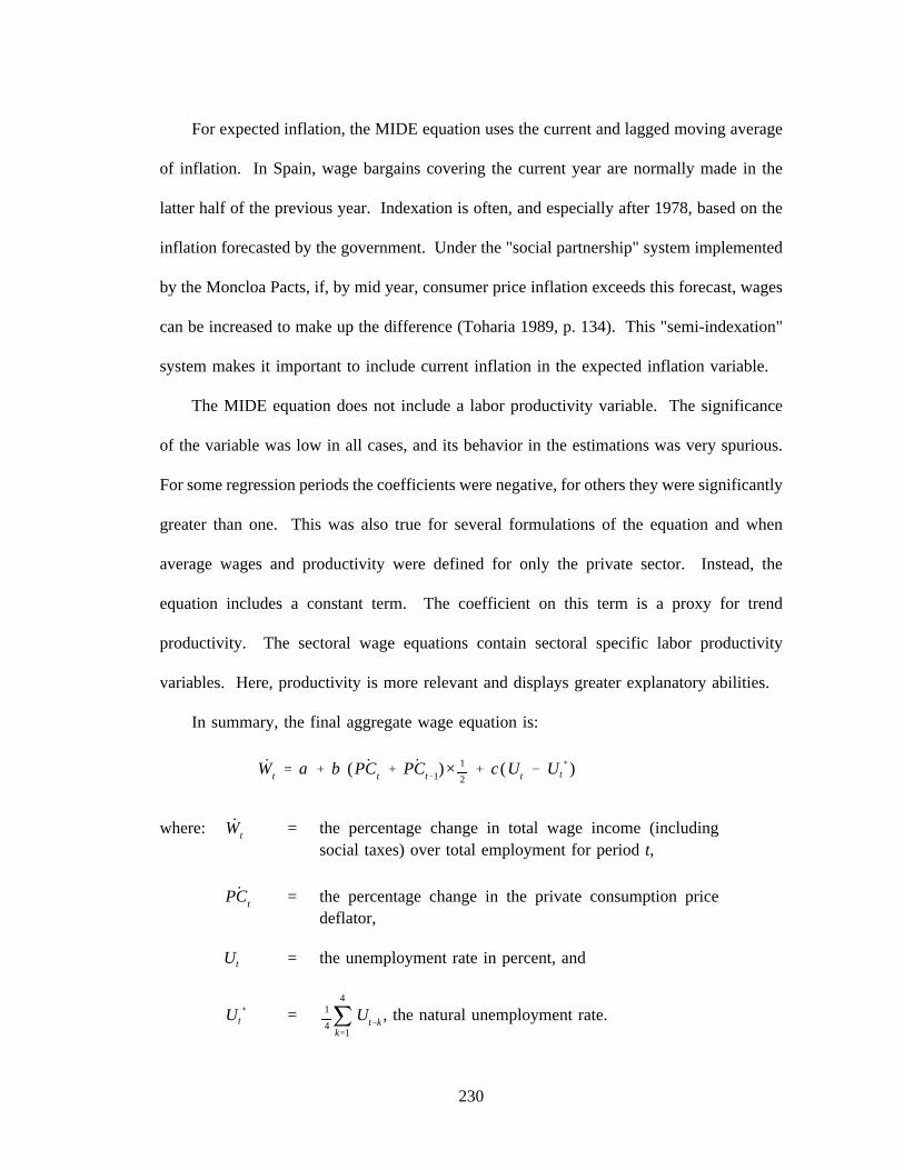
For expected inflation, the MIDE equation uses the current and lagged moving average
of inflation. In Spain, wage bargains covering the current year are normally made in the
latter half of the previous year. Indexation is often, and especially after 1978, based on the
inflation forecasted by the government. Under the "social partnership" system implemented
by the Moncloa Pacts, if, by mid year, consumer price inflation exceeds this forecast, wages
can be increased to make up the difference (Toharia 1989, p. 134). This "semi-indexation"
system makes it important to include current inflation in the expected inflation variable.
The MIDE equation does not include a labor productivity variable. The significance
of the variable was low in all cases, and its behavior in the estimations was very spurious.
For some regression periods the coefficients were negative, for others they were significantly
greater than one. This was also true for several formulations of the equation and when
average wages and productivity were defined for only the private sector. Instead, the
equation includes a constant term. The coefficient on this term is a proxy for trend
productivity. The sectoral wage equations contain sectoral specific labor productivity
variables. Here, productivity is more relevant and displays greater explanatory abilities.
In summary, the final aggregate wage equation is:
Wt a b ( ˙PCt˙PCt 1)× 1
2c (Ut Ut )
where: = the percentage change in total wage income (includingWt
social taxes) over total employment for period t,
= the percentage change in the private consumption price˙PCt
deflator,
Ut = the unemployment rate in percent, and
= , the natural unemployment rate.Ut1
4
4
k 1
Ut k
230

In order to assure reasonable long-run properties, the coefficient on the inflation
expectation term is softly constrained to equal one. Figure 7.3 displays the regression
results. The equation provides a reasonable explanation Spanish wages for the period
covering the 70’s and 80’s. However, as one might expect given the history of Spanish
wage formation sketched above, the magnitude of the regression coefficients and the
goodness of fit are highly sensitive to the estimation period.
The first regression shown in Figure 7.3 covers the period of 1970 through 1990.
Indexation dominated wage formation in the 70s, and labor successfully resisted decreases
in real wage growth despite decreases in labor productivity growth. Because of this "real
wage rigidity" the equation yields an unconstrained coefficient on inflation expectations of
1.25. The intercept parameter of the unconstrained equation is only 2.62, close to the
average productivity growth rate of the period, which was 3.08 percent. The constraint
required to obtain an inflation coefficient equal to one in this equation was very hard, and
the intercept receives the bulk of the explanatory power. The coefficient on the intercept,
4.7, exceeds the average productivity growth by a large margin. Moreover, the equation
fails miserably in explaining wage inflation in the 80’s.
As stressed above, the transformation of labor relations, initiated by the transition to
democracy and the Moncloa pacts, produced important changes for wage setting in the
Spanish economy. This clear break in behavior mandates the use of an equation estimated
over a more recent period. The second regression displayed in Figure 7.3 displays the
equation estimated from 1980-90. The fit of the equation is much better and the data more
readily accepts the constraint on the inflation parameter (the trade-off of the fit to conformity
of the constraint is 10 times less). The average productivity growth during the period was
2.27, the coefficient on the intercept is one point below this.
231

Figure 7.3: Estimation Results for Aggregate Wage Equation.
Equation 1: 1970 - 1990SEE = 3.77 RSQ = 0.64 RHO = 0.88SEE+1 = 1.99 RBSQ = 0.60 DW = 0.24MAPE = 26.73 Obser = 21 DoFree = 18
Variable name Reg-Coef Mexval t-value Mean0 Avg. Wage (% change) - - - - - - - - - - - - - - 15.791 intercept 4.700 28.9 3.47 1.002 Inflation (2yr. ma.) 1.033 * * 11.903 Unrat. - Nat Unrat. -0.612 8.4 -1.78 1.94
Equation 2: 1980 - 1990, no dummySEE = 0.94 RSQ = 0.92 RHO =-0.42SEE+1 = 0.84 RBSQ = 0.90 DW = 2.83MAPE = 7.89 Obser = 11 DoFree = 8
Variable name Reg-Coef Mexval t-value Mean0 Avg. Wage (% change) - - - - - - - - - - - - - - 11.051 intercept 1.026 8.4 1.19 1.002 Inflation (2yr. ma.) 1.031 * * 10.403 Unrat. - Nat Unrat. -0.318 31.3 -2.42 2.22
Equation 3: 1980 - 1990, with dummySEE = 0.51 RSQ = 0.98 RHO = -0.27SEE+1 = 0.48 RBSQ = 0.96 DW = 2.54MAPE = 3.70 Obser = 11 DoFree = 7
Variable name Reg-Coef Mexval t-value Mean0 Avg. Wage (% change) - - - - - - - - - - - - - - 11.051 intercept 1.693 57.6 3.22 1.002 Inflation (2yr. ma.) 0.995 * * 10.403 Unrat. - Nat Unrat. -0.274 67.7 -3.56 2.224 Dummy 84 & 87 -2.103 85.3 -4.13 0.18
* - indicates constrained coefficient.
Predicted vs. Actual, 1980-90 w/dummy
232

The third equation of Figure 7.3 is the same as the second with one modification, a
dummy variable to account for two years where economy-wide wage agreements were not
in effect. The first one was 1984. Curiously, nominal wage growth fell precipitously in that
year. In mid-1984, an agreement was signed covering 1985-86. Since then, no agreement
has been in force. The first year of the latter period, 1987, also saw a steep fall in nominal
wages. The inclusion of the dummy variable cuts the mean absolute percentage error
(MAPE) by over four points. It also increases the intercept term so that it is now closer to
average productivity growth. This is the equation used in the MIDE model.
Sectoral Wage Equations
To determine industry level wages and salaries (gross employment income, including
social security taxes paid by the employer), the MIDE model computes an index for wages
by employee (1980 = 1.0), converts this index to current price pesetas, and multiplies this
amount by the number of employees. The explanatory variables for each of the index
equations is the aggregate wage compensation index and the sectoral labor productivity per
worker. Specifically:
ln
Wi,t /Li,t
Wi,80 /Li,80
ai bi ln
Wt /Lt
W80 /L80
ci ln
Qi,t
Li,t
where: Wi,t = total employment income for sector i and period t,
Li,t = employment in persons,
Wt = aggregate employment income,
Lt = aggregate employment in persons,
Qi,t = output of sector i in period.
233
The regression results are displayed in Table 7.1. If the industry level productivity variable
yielded a negative coefficient, it was left out of the equation. This occurs for three sectors,
Electricity (Sector 5), Beverages (18) and Construction (26). According to the R-squares
and t-statistics displayed by these results, the aggregate wage index goes a long way toward
explaining the behavior of sectoral wages. This is consistent with the conclusions of Viñals
et al. (1989, p. 170).
7.2 Capital Income
The second component of industry value added in the MIDE model is capital income,
or gross profits, for both corporations and proprietors. A large portion of capital income is
net profits which tends to be cyclically volatile. It also includes more stable items such as
capital consumption, net interest payments by business, business transfer payments (pension
and severance benefits), and rental income (including the imputed rent from owner-occupied
dwellings). Net interest and depreciation move fairly steadily over the business cycle.
Profits and proprietor income, on the other hand, are prime indicators of business cycle
movement. Therefore, it is normally appropriate to model these components separately
(Monaco 1991). However, since the available data does not provide the allocation of these
parts at a sectoral level, the MIDE model includes industry level equations for total capital
income. Capital consumption, interest and transfer payments are then modeled at the
aggregate level.
Unlike labor compensation, profit movements are not uniform across branches of
activity. Moreover, the factors affecting profits vary across industries. This fact emphasizes
the vital role that profits play in the MIDE model. Recall that, through the sectoral price
identity, the various components of value added are an integral part of price determination.
234

Table 7.1: Summary of Sectoral Wage Equations.(t statistics in parentheses)
sectoraggreg. labor
const wage prod. rho rbsq(a) (b) (c)
1. Agric, f & f2. Coal3. Coke4. Petroleum5. Electricity
6. Met mng, proc7. Nmet prod8. Chemicals9. Met prod
10. Ind mach
11. Off mach12. Elect prod13. Motor veh14. Oth tran eq15. Meat prod
16. Dairy prod17. Oth food18. Beverages19. Tobacco20. Text & app
21. Leather prod22. Wood prod23. Pap & publ24. Rub & plas25. Oth mfg prod
26. Construction27. Rep & reconst28. Trade29. Rest & hotels30. Int transport
31. Marit & air32. Transp serv33. Communic34. Bank & insur35. Bus serv
36. Rents37. Priv educ38. Priv health39. Oth serv
40. Publ adm41. Publ educ42. Publ health43. Dom serv
-1.938 (112.) 0.721 (13.7) 0.819 ( 7.5) -.46 .990.137 ( 1.0) 0.945 (16.1) 0.209 ( 1.5) .35 .99
-1.026 ( 1.2) 0.968 (13.2) 0.430 ( 1.6) -.17 .97-1.665 ( 1.9) 0.776 ( 7.6) 0.479 ( 2.3) .31 .920.376 (21.2) 1.092 (29.9) .20 .99
-1.760 ( 4.2) 0.694 (13.7) 0.872 ( 5.3) .03 .99-0.783 ( 1.0) 0.759 ( 3.4) 0.554 ( 0.7) -.31 .99-0.831 ( 3.7) 0.841 (12.0) 0.504 ( 3.5) -.19 .99-1.030 (12.7) 0.788 (72.9) 0.840 ( 9.8) -.38 .99-0.927 ( 6.0) 0.717 (13.3) 0.713 ( 6.1) .48 .99
-0.657 ( 1.9) 0.452 ( 1.3) 0.486 ( 2.0) .23 .90-0.661 ( 2.5) 0.846 ( 8.3) 0.559 ( 2.5) .41 .98-0.524 ( 2.4) 0.773 (10.1) 0.423 ( 3.0) -.13 .99-0.558 ( 4.3) 0.318 ( 3.6) 0.631 ( 4.4) .41 .94-1.767 ( 1.4) 0.859 (17.0) 0.736 ( 1.4) .16 .98
-0.868 ( 1.1) 0.663 (15.9) 0.423 ( 1.2) .30 .97-1.150 ( 3.3) 0.891 (13.4) 0.401 ( 1.8) -.67 .99-0.068 ( 4.9) 1.090 (38.4) .10 .99-4.339 ( 1.2) 0.707 ( 1.1) 1.976 ( 1.2) -.04 .82-1.448 (10.6) 0.679 (17.0) 1.166 ( 5.0) .17 .99
-1.056 (21.3) 0.776 (13.9) 0.670 ( 7.0) -.20 .99-1.102 (19.3) 0.668 (39.0) 0.732 ( 7.0) -.13 .99-0.817 ( 4.4) 0.917 (13.6) 0.447 ( 2.7) -.15 .99-1.108 ( 6.5) 0.834 ( 9.6) 0.843 ( 5.5) -.44 .99-1.288 (10.9) 0.782 ( 4.2) 0.549 ( 2.7) .04 .98
-0.150 ( 9.1) 0.726 (21.6) .33 .99-1.158 ( 7.4) 0.627 ( 7.0) 0.791 ( 3.3) -.34 .98-0.940 ( 6.8) 0.806 (16.1) 0.246 ( 0.8) -.22 .99-0.941 ( 2.7) 0.972 (29.4) 0.144 ( 0.5) .12 .99-1.396 ( 4.5) 0.411 ( 1.6) 1.591 ( 2.7) .51 .98
-1.108 ( 1.5) 0.539 ( 3.1) 0.952 ( 2.1) .69 .93-0.399 ( 3.6) 1.037 (15.7) 0.273 ( 2.2) .00 .99-0.446 ( 4.7) 0.703 (19.6) 0.708 ( 6.7) .06 .99-0.252 ( 0.4) 1.130 (13.6) 0.525 ( 1.1) -.17 .99-1.335 (39.8) 1.031 (107.) 0.786 (40.5) -.60 .99
-4.987 (57.3) 0.927 (54.4) 1.028 (76.5) -.04 .990.170 ( 2.7) 0.859 (21.4) 0.641 ( 2.1) .29 .99
-1.214 (14.5) 1.111 (46.1) 1.052 ( 8.4) -.50 .99-0.683 ( 4.4) 1.485 (44.4) 0.551 ( 1.7) -.17 .99
-0.348 ( 3.2) 0.693 (37.5) 0.962 ( 7.1) -.34 .99-0.010 ( 0.2) 0.985 (22.9) 0.296 ( 0.9) .25 .990.023 ( 0.1) 0.836 (13.5) 0.636 ( 2.0) .04 .96
-0.286 ( 1.0) 0.818 (57.1) 0.839 ( 3.0) .05 .99
235
In the Spanish economy, uniformity of wage growth across sectors suggests that, to a great
extent, wages determine the general price level. The heterogeneity of profit movements, on
the other hand, means that sectoral level profit margins help to define relative prices.
Monaco (1991) presents recent work describing the specification of profit equations for
a macroeconomic, multisectoral model of the United States. Her approach is to depict profit
behavior as a "mark-up" over unit costs. Monaco explains that several other multisectoral
and macroeconomic models use such an approach to model prices, and, therefore it is a
useful context to model profits. In her work, sectoral, real profit margins are functions of
material input prices, labor costs and demand. For various reasons, I had tremendous
difficulties with implementing this approach here. First of all, degrees of freedom
limitations prohibited the full use of Monaco’s specification. It was difficult to incorporate
lags representing the pass-through of labor costs, since sectoral employment compensation
was available only since 1980. Also, the equations here do not contain material input
explanatory variables (except in one special case).
Secondly, Monaco’s dependent variable for the equations is deflated profits over output.
To form this variable, the nominal profits are deflated by an industry-specific price index.
Since profits are a partial determinant of prices, however, deflating profits by the current
year’s price index raises a simultaneity issue in the overall model specification.
Consequently, profits are deflated with the previous period’s output deflator. However, the
use of this technique for the Spanish equations yielded very unsatisfactory results. Ignoring
the simultaneity in estimation problem, I attempted to construct the dependent variable using
the current period industry level price deflator, as well as the GDP deflator, for deflating the
profits. The equations generated by this approach were generally very good. However, the
236

use of the current year’s deflator introduced severe convergence problems inside the price-
income block.
The final solution is to estimate the profit margin not as a proportion of output, but as
a proportion of value added at factor cost (gross profits plus gross employment income).2
This approach eliminates the need for profit deflation. However, it limits the interpretation
of the profit margin as a mark-up over labor costs, rather than all of intermediate costs.
Specifically, the definition of the dependent variable is:
PSHVAi,t
PROFi,t
PROFi,t WAGi,t
× 100
where: PSHVAi,t = profit share of value added at factor costfor sector i in period t,
PROFi,t = nominal gross profits,
WAGi,t = nominal gross wages and salaries.
Obviously, one determinate of industry profits is growth in the level of demand. Like
prices, profits are sensitive to demand changes and normally exhibit strongly pro-cyclical
behavior. The profit equations of the MIDE model use either the current or a two period
moving average of the percentage change in output, depending on which provides the better
results. Specifically, the cyclical variable is defined as:
PCQi,t
si ×(Qi,t Qi,t 1)
Qi,t 1
(1 si) ×(Qi,t 1 Qi,t 2)
Qi,t 2
× 100
where: Qi,t = constant price output, and
2 This idea was borrowed from Shackleton (1992), who experienced very similarproblems for the construction of the INFORUM United Kingdom model.
237

si = is either .5 or 1.0.
Another explanatory factor significant in each sector is the real unit labor cost. An
increase in labor costs may temporarily squeeze profit shares if the increase cannot be passed
on through a price increase. The strength of the effect on profits in an individual industry
will depend on its competitive structure, openness to international trade, as well as demand
conditions. In an oligopolistic industry, for instance, individual firms may be unwilling to
pass cost increases on to consumers for fear of losing market share. Instead, and for a time,
the oligopolist absorbs part of the increase by decreasing profit margins. Therefore, higher
unit wage costs lead to lower shares of value added in the short run. On the other hand,
labor productivity increases which reduce the unit labor cost lead to larger profit shares until
the productivity increases are compensated with equivalent wage increases. To form current
price unit wage cost, the gross employment income of each sector is divided by real output.
For non-tradeable goods sectors, an appropriate deflator for this quantity is the GDP deflator.
(Use of the sectoral own price deflator introduces estimation and convergence simultaneity
problems similar to those discussed above.) Therefore, the real unit labor cost is essentially:
RLCi,t
(WAGi,t /Qi,t)
PGDPt
where: RLCi,t = the real unit wage cost of sector i in period t,
WAGi,t = nominal gross wages and salaries.
Qi,t = constant price output, and
PGDPt = the GDP deflator.
For tradable sectors, however, we can integrate another important determinate of profit
shares into a single explanatory variable.
238

In a small open economy, often the most important determinate or relative prices is
whether a good is tradeable or non-tradeable. In most theoretical and many empirical
models, the price of tradeable goods is assumed equal to the world price of these goods.
Current developments in the Spanish economy, as discussed in Chapter 2, illustrate that the
tradeable/non-tradable distinction is indeed important. Over the past several years,
manufacturing industries, open to world trade, have experienced substantially less price
inflation than the non-tradable service sectors. Schultz (1986) found that the ratio of the
import price to unit wage costs, the real exchange rate, are very important for explaining
profit margins for European countries. Therefore, in the MIDE model, profit share equations
for several of the tradable goods industries include a real exchange rate, defined as:
RERi,t
(PMi,t(1 TMi,t)
(WAGi,t/Qi,t)
RERi,t = the real exchange rate for sector i at period t,
PMi,t = the import price at the border,
TMi,t = the import tax rate, and
WAGi,t = nominal gross wages and salaries, and
Qi,t = constant price output.
This coefficient on this variable is expected to be positive, since higher foreign prices (or
tariff rates) imply greater accommodation for domestic (or export) price increases and,
therefore, higher profit shares. An increase in unit labor costs reduces the magnitude of the
real exchange rate, acting to reduce the profit share. As displayed below, for most of the
239

Spanish manufacturing industries, the real exchange rate is indeed a powerful explanatory
variable.
In summary, the specification for the profit equations is:
PVASHi,t ai bi PCQi,t ci
RLCi,t
RERi,t
di OTHi,t
where OTHi,t represents other independent variables included in the specification. Table 7.2
displays the results for the 38 sectors estimated with this form. Examination of the
individual equations reveals that the real exchange rate is included for the majority of
manufactured sectors. However, for energy (2, 3 and 5) and food (15, 16, 17 and 18)
sectors the real labor cost explains profit share movements much better. In each of these
cases, imports shares of demand are either zero or trivial.
Dummy variables for obvious outliers in the series are included for equations that yield
unreasonable parameter values without the dummy. (In Table 7.2 the range of years where
the dummy is equal to one is shown. For all other years, the dummy variable is equal to
zero.) For several sectors (1, 3, 6, 8, 13 and 18), the dummy starts in 1985 or 1986 and
continues to assume the value of one for forecasting. The significance of the parameter in
these cases could be due to a number of reasons. First, changes in tax and subsidy regimes
as a result of EC integration could have had an impact. Possibly, the elimination of the
cascade tax (see Chapter 5) improve the profit shares of intermediate goods industries such
as Coke products (Sector 3), Base metals (6) and Chemicals (8). Profits in agriculture
apparently benefitted from the introduction of the Common Agriculture Policy (CAP). On
the other hand, the change in the national accounts data from the 1980 base to the 1986 base
240

affected value added data substantially (see Appendix). These dummies may be signalling
inconsistencies in the profits data resulting from this problem.
In Spain, the Petroleum products industry (Sector 4) is essentially refining and
distribution. Domestic prices for its products are highly regulated by the government.
Therefore, its profits should be sensitive to the relative price of imported petroleum.
Including this variable (price imports for sector 4 over the GDP deflator) in the profit share
equation does not add significantly to the explanatory power of the equation, bad in any
case, but does help explain a wiggle in 1986-87.
Soft constraints were used on the equations for sectors 8 and 25 to give positive
parameters on the change of output term. For sectors 7, 23 and 24 constraints are used to
yield coefficients on output growth to be less than one. While there is no a-priori reason
to believe that a parameter greater than one would be inappropriate, model simulations
revealed that such a value resulted in excess volatility in the profit share. For similar
stability reasons, a soft constraint on the equation for sector 25 reduces the magnitude of the
real exchange rate parameter. A constraint on the equation for sector 29 reduces the real
labor cost parameter. A final manipulation required to reach reasonable fits and parameter
results for various equations (sectors 3, 5, 9, 23) was to start the estimation period in 1981
rather than 1980. For Hotels, bars and restaurants (sector 29) the final estimation period is
1983 through 1987. Since this equation also contains a dummy variable and soft constraints,
it is evident that the final result is highly administered. In fact, it was very difficult to
estimate an equation for this sector which behaved well in the full model. Since profits of
this sector constitute close to ten percent of total economy-wide profits, the high-handed
treatment of the sector is essential for satisfactory overall behavior of the model.
241

Table 7.2: Estimation results for sectoral gross profit equations:Manufacturing and private services.
1. Agriculture, forestry & fisheriesSEE = 0.53 RSQ = 0.8804 RHO = -0.43 Obser = 8 from 1980SEE+1 = 0.47 RBSQ = 0.7907 DW = 2.86 DoFree = 4 to 1987MAPE = 0.60
Variable name Reg-Coef Mexval t-value Elas Mean0 pshva1 - - - - - - - - - - - - - - - - - - - - - 73.351 intercept 65.07905 1183.0 25.581 0.89 1.002 pcq1 (s=1.0) 0.11062 38.8 1.924 0.00 2.033 rer1 6.52036 77.3 2.927 0.10 1.124 dum86_87 3.06146 158.4 4.765 0.01 0.25
2. Coal & radioactive materialSEE = 3.43 RSQ = 0.4755 RHO = 0.22 Obser = 8 from 1980SEE+1 = 3.49 RBSQ = 0.2657 DW = 1.55 DoFree = 5 to 1987MAPE = 14.76
Variable name Reg-Coef Mexval t-value Elas Mean0 pshva2 - - - - - - - - - - - - - - - - - - - - - 23.031 intercept 38.73000 31.9 1.923 1.68 1.002 pcq2 (s=0.5) 0.38313 37.6 2.114 0.12 7.213 rlc2 -22.29840 7.6 -0.890 -0.80 0.83
3. Coke productsSEE = 1.70 RSQ = 0.8656 RHO = 0.06 Obser = 7 from 1981SEE+1 = 1.70 RBSQ = 0.7985 DW = 1.88 DoFree = 4 to 1987MAPE = 1.65
Variable name Reg-Coef Mexval t-value Elas Mean0 pshva3 - - - - - - - - - - - - - - - - - - - - - 82.661 intercept 110.11061 267.8 7.079 1.33 1.002 rlc3 -30.90491 39.0 -1.931 -0.36 0.973 dum86_87 8.35429 142.4 4.415 0.03 0.29
4. Petroleum extraction & refiningSEE = 7.74 RSQ = 0.1563 RHO = -0.19 Obser = 8 from 1980SEE+1 = 7.56 RBSQ =-0.1812 DW = 2.38 DoFree = 5 to 1987MAPE = 8.76
Variable name Reg-Coef Mexval t-value Elas Mean0 pshva4 - - - - - - - - - - - - - - - - - - - - - 74.881 intercept 80.42492 223.0 6.867 1.07 1.002 pcq4 (s=1.0) 0.41867 4.4 0.674 0.00 0.823 rpmoil -5.50427 2.8 -0.532 -0.08 1.07
5. Electricity, gas transmission & water utilities
SEE = 1.39 RSQ = 0.8835 RHO = -0.68 Obser = 7 from 1981SEE+1 = 0.92 RBSQ = 0.8252 DW = 3.36 DoFree = 4 to 1987MAPE = 1.78
Variable name Reg-Coef Mexval t-value Elas Mean0 pshva5 - - - - - - - - - - - - - - - - - - - - - 68.151 intercept 110.28468 470.9 11.242 1.62 1.002 pcq5 (s=1.0) 0.61594 19.7 1.316 0.03 2.843 rlc5 -42.17133 156.1 -4.715 -0.64 1.04
242
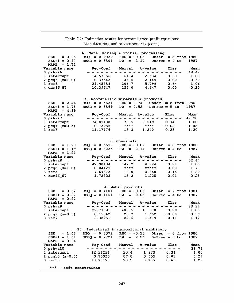
Table 7.2: Estimation results for sectoral gross profit equations:Manufacturing and private services (cont.).
6. Metal mining & initial processingSEE = 0.98 RSQ = 0.9029 RHO = -0.08 Obser = 8 from 1980SEE+1 = 0.97 RBSQ = 0.8301 DW = 2.17 DoFree = 4 to 1987MAPE = 1.72
Variable name Reg-Coef Mexval t-value Elas Mean0 pshva6 - - - - - - - - - - - - - - - - - - - - - 48.421 intercept 14.53856 61.4 2.534 0.30 1.002 pcq6 (s=1.0) 0.37642 46.6 2.145 0.00 0.303 rer6 29.45589 206.7 5.799 0.64 1.064 dum86_87 10.39647 153.0 4.647 0.05 0.25
7. Nonmetallic minerals & productsSEE = 2.46 RSQ = 0.5621 RHO = 0.74 Obser = 8 from 1980SEE+1 = 1.78 RBSQ = 0.3869 DW = 0.52 DoFree = 5 to 1987MAPE = 4.99
Variable name Reg-Coef Mexval t-value Elas Mean0 pshva7 - - - - - - - - - - - - - - - - - - - - - 47.201 intercept 34.85188 70.5 3.219 0.74 1.002 pcq7 (s=0.5) 0.72936 **** **** -0.02 -1.483 rer7 11.17776 13.3 1.240 0.28 1.20
8. ChemicalsSEE = 1.20 RSQ = 0.5558 RHO = -0.07 Obser = 8 from 1980SEE+1 = 1.19 RBSQ = 0.2226 DW = 2.14 DoFree = 4 to 1987MAPE = 1.81
Variable name Reg-Coef Mexval t-value Elas Mean0 pshva8 - - - - - - - - - - - - - - - - - - - - - 52.671 intercept 42.90134 142.2 4.724 0.81 1.002 pcq8 (s=1.0) 0.04125 **** ***** 0.00 1.773 rer8 7.69272 10.0 0.980 0.18 1.204 dum86_87 1.72323 15.2 1.225 0.01 0.25
9. Metal productsSEE = 0.32 RSQ = 0.4101 RHO = -0.03 Obser = 7 from 1981SEE+1 = 0.32 RBSQ = 0.1151 DW = 2.05 DoFree = 4 to 1987MAPE = 0.82
Variable name Reg-Coef Mexval t-value Elas Mean0 pshva9 - - - - - - - - - - - - - - - - - - - - - 33.321 intercept 29.73391 487.5 11.578 0.89 1.002 pcq9 (s=0.5) 0.15842 29.7 1.652 -0.00 -0.993 rer9 3.32951 22.6 1.419 0.11 1.12
10. Industrial & agricultural machinerySEE = 1.68 RSQ = 0.8372 RHO = -0.13 Obser = 8 from 1980SEE+1 = 1.61 RBSQ = 0.7721 DW = 2.26 DoFree = 5 to 1987MAPE = 3.66
Variable name Reg-Coef Mexval t-value Elas Mean0 pshva10 - - - - - - - - - - - - - - - - - - - - - 36.751 intercept 12.31251 30.4 1.870 0.34 1.002 pcq10 (s=0.5) 0.73323 87.8 3.555 0.01 0.293 rer10 18.73155 93.5 3.705 0.66 1.29
*** - soft constraints
243

Table 7.2: Estimation results for sectoral gross profit equations:Manufacturing and private services (cont.).
11. Office machines, computers and precision instrumentsSEE = 5.49 RSQ = 0.8974 RHO = 0.28 Obser = 8 from 1980SEE+1 = 5.58 RBSQ = 0.8803 DW = 1.45 DoFree = 6 to 1987MAPE = 9.86
Variable name Reg-Coef Mexval t-value Elas Mean0 pshva11 - - - - - - - - - - - - - - - - - - - - - 50.811 intercept -1.08028 0.2 -0.144 -0.02 1.002 rer11 32.34795 212.2 7.244 1.02 1.60
12. Electrical & electronic equip.SEE = 1.85 RSQ = 0.6395 RHO = 0.27 Obser = 8 from 1980SEE+1 = 1.79 RBSQ = 0.4952 DW = 1.47 DoFree = 5 to 1987MAPE = 4.28
Variable name Reg-Coef Mexval t-value Elas Mean0 pshva12 - - - - - - - - - - - - - - - - - - - - - 34.021 intercept 28.94247 56.5 2.692 0.85 1.002 pcq12 (s=1.0) 0.39576 64.9 2.932 0.04 3.373 rer12 3.36551 1.2 0.349 0.11 1.11
13. Motor vehicles & enginesSEE = 1.20 RSQ = 0.9844 RHO = -0.25 Obser = 8 from 1980SEE+1 = 1.13 RBSQ = 0.9727 DW = 2.49 DoFree = 4 to 1987MAPE = 3.56
Variable name Reg-Coef Mexval t-value Elas Mean0 pshva13 - - - - - - - - - - - - - - - - - - - - - 31.691 intercept 15.02306 69.6 2.739 0.47 1.002 pcq13 (s=1.0) 0.34312 101.3 3.494 0.05 5.043 rer13 7.07049 25.3 1.510 0.28 1.284 dum85_87 15.76600 451.6 10.849 0.19 0.37
14. Other transport equipmentSEE = 3.76 RSQ = 0.9205 RHO = 0.32 Obser = 8 from 1980SEE+1 = 3.83 RBSQ = 0.9072 DW = 1.35 DoFree = 6 to 1987MAPE =13.43
Variable name Reg-Coef Mexval t-value Elas Mean0 pshva14 - - - - - - - - - - - - - - - - - - - - - 33.411 intercept -11.68143 31.1 -2.077 -0.35 1.002 rer14 22.10257 254.6 8.334 1.35 2.04
15. Meat & other animal productsSEE = 0.45 RSQ = 0.9782 RHO = 0.06 Obser = 8 from 1980SEE+1 = 0.45 RBSQ = 0.9619 DW = 1.87 DoFree = 4 to 1987MAPE = 0.67
Variable name Reg-Coef Mexval t-value Elas Mean0 pshva15 - - - - - - - - - - - - - - - - - - - - - 57.551 intercept 106.42729 328.7 8.337 1.85 1.002 pcq15 (s=1.0) 0.33648 37.6 1.890 0.01 1.243 rlc15 -48.14732 115.4 -3.816 -0.83 -1.004 dum80_81 -4.98239 377.9 -9.346 -0.02 0.25
244
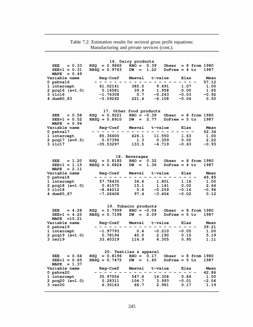
Table 7.2: Estimation results for sectoral gross profit equations:Manufacturing and private services (cont.).
16. Dairy productsSEE = 0.33 RSQ = 0.9865 RHO = 0.39 Obser = 8 from 1980SEE+1 = 0.31 RBSQ = 0.9763 DW = 1.22 DoFree = 4 to 1987MAPE = 0.49
Variable name Reg-Coef Mexval t-value Elas Mean0 pshva16 - - - - - - - - - - - - - - - - - - - - - 57.121 intercept 61.02141 385.0 9.491 1.07 1.002 pcq16 (s=1.0) 0.16581 39.9 1.958 0.00 1.653 rlc16 -1.76308 0.7 -0.243 -0.03 -0.924 dum80_83 -5.09292 221.4 -6.108 -0.04 0.50
17. Other food productsSEE = 0.58 RSQ = 0.9221 RHO = -0.39 Obser = 8 from 1980SEE+1 = 0.52 RBSQ = 0.8910 DW = 2.77 DoFree = 5 to 1987MAPE = 0.94
Variable name Reg-Coef Mexval t-value Elas Mean0 pshva17 - - - - - - - - - - - - - - - - - - - - - 52.341 intercept 85.36600 426.1 11.550 1.63 1.002 pcq17 (s=0.5) 0.07396 1.3 0.359 0.00 2.223 rlc17 -35.53297 133.5 -4.719 -0.63 -0.93
18. BeveragesSEE = 1.20 RSQ = 0.8185 RHO = 0.32 Obser = 8 from 1980SEE+1 = 1.15 RBSQ = 0.6824 DW = 1.36 DoFree = 4 to 1987MAPE = 2.11
Variable name Reg-Coef Mexval t-value Elas Mean0 pshva18 - - - - - - - - - - - - - - - - - - - - - 49.851 intercept 57.78435 34.6 1.801 1.16 1.002 pcq18 (s=1.0) 0.41575 15.1 1.141 0.02 2.643 rlc18 -8.44212 0.8 -0.259 -0.16 -0.964 dum85_87 -7.26408 97.4 -3.404 -0.02 0.12
19. Tobacco productsSEE = 4.28 RSQ = 0.7999 RHO = -0.04 Obser = 8 from 1980SEE+1 = 4.25 RBSQ = 0.7198 DW = 2.09 DoFree = 5 to 1987MAPE =10.21
Variable name Reg-Coef Mexval t-value Elas Mean0 pshva19 - - - - - - - - - - - - - - - - - - - - - 39.211 intercept -1.97793 0.4 -0.210 -0.05 1.002 pcq19 (s=1.0) 0.78194 40.0 2.190 0.10 5.193 rer19 33.40319 116.9 4.305 0.95 1.11
20. Textiles & apparelSEE = 0.64 RSQ = 0.8196 RHO = 0.17 Obser = 8 from 1980SEE+1 = 0.65 RBSQ = 0.7475 DW = 1.65 DoFree = 5 to 1987MAPE = 1.37
Variable name Reg-Coef Mexval t-value Elas Mean0 pshva20 - - - - - - - - - - - - - - - - - - - - - 42.861 intercept 35.97056 547.6 14.308 0.84 1.002 pcq20 (s=1.0) 0.28311 104.7 3.993 -0.01 -2.063 rer20 6.30163 66.7 2.981 0.17 1.19
245
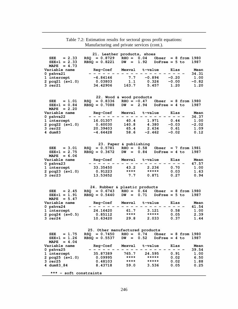
Table 7.2: Estimation results for sectoral gross profit equations:Manufacturing and private services (cont.).
21. Leather products, shoesSEE = 2.33 RSQ = 0.8729 RHO = 0.04 Obser = 8 from 1980SEE+1 = 2.33 RBSQ = 0.8221 DW = 1.92 DoFree = 5 to 1987MAPE = 4.73
Variable name Reg-Coef Mexval t-value Elas Mean0 pshva21 - - - - - - - - - - - - - - - - - - - - - 34.311 intercept -6.84146 7.7 -0.894 -0.20 1.002 pcq21 (s=1.0) 0.03803 1.1 0.326 -0.00 -0.823 rer21 34.42906 163.7 5.457 1.20 1.20
22. Wood & wood productsSEE = 1.01 RSQ = 0.8336 RHO = -0.47 Obser = 8 from 1980SEE+1 = 0.84 RBSQ = 0.7088 DW = 2.94 DoFree = 4 to 1987MAPE = 2.20
Variable name Reg-Coef Mexval t-value Elas Mean0 pshva22 - - - - - - - - - - - - - - - - - - - - - 36.371 intercept 16.01307 40.4 1.971 0.44 1.002 pcq22 (s=1.0) 0.60030 140.8 4.380 -0.03 -2.023 rer22 20.39403 65.4 2.634 0.61 1.094 dum83 -4.64428 58.6 -2.462 -0.02 0.12
23. Paper & publishingSEE = 3.01 RSQ = 0.5781 RHO = 0.58 Obser = 7 from 1981SEE+1 = 2.75 RBSQ = 0.3672 DW = 0.84 DoFree = 4 to 1987MAPE = 6.06
Variable name Reg-Coef Mexval t-value Elas Mean0 pshva23 - - - - - - - - - - - - - - - - - - - - - 47.571 intercept 33.35450 43.2 2.236 0.70 1.002 pcq23 (s=1.0) 0.91223 **** ***** 0.03 1.633 rer23 13.53652 7.7 0.871 0.27 0.94
24. Rubber & plastic productsSEE = 2.45 RSQ = 0.6743 RHO = 0.64 Obser = 8 from 1980SEE+1 = 1.91 RBSQ = 0.5440 DW = 0.71 DoFree = 5 to 1987MAPE = 5.47
Variable name Reg-Coef Mexval t-value Elas Mean0 pshva24 - - - - - - - - - - - - - - - - - - - - - 41.541 intercept 24.16420 61.7 3.121 0.58 1.002 pcq24 (s=0.5) 0.85112 **** ***** 0.05 2.393 rer24 10.63420 29.8 2.033 0.37 1.44
25. Other manufactured productsSEE = 1.75 RSQ = 0.7450 RHO = 0.74 Obser = 8 from 1980SEE+1 = 1.26 RBSQ = 0.5537 DW = 0.52 DoFree = 4 to 1987MAPE = 4.04
Variable name Reg-Coef Mexval t-value Elas Mean0 pshva25 - - - - - - - - - - - - - - - - - - - - - 39.541 intercept 35.87389 765.7 24.595 0.91 1.002 pcq25 (s=1.0) 0.09995 **** ***** 0.02 6.503 rer25 0.48103 **** ***** 0.02 1.884 dum83_84 8.43718 59.0 3.536 0.05 0.25
*** - soft constraints
246

Table 7.2: Estimation results for sectoral gross profit equations:Manufacturing and private services (cont.).
26. ConstructionSEE = 1.11 RSQ = 0.9508 RHO = -0.12 Obser = 8 from 1980SEE+1 = 1.09 RBSQ = 0.9311 DW = 2.23 DoFree = 5 to 1987MAPE = 2.61
Variable name Reg-Coef Mexval t-value Elas Mean0 pshva26 - - - - - - - - - - - - - - - - - - - - - 33.501 intercept 70.00210 531.0 13.932 2.09 1.002 pcq26 (s=1.0) 0.00180 0.0 0.016 0.00 1.203 rlc26 -42.93546 247.1 -7.431 -1.09 -0.85
27. Repairs & reconstructionSEE = 0.88 RSQ = 0.9052 RHO = 0.32 Obser = 8 from 1980SEE+1 = 0.89 RBSQ = 0.8894 DW = 1.35 DoFree = 6 to 1987MAPE = 1.33
Variable name Reg-Coef Mexval t-value Elas Mean0 pshva27 - - - - - - - - - - - - - - - - - - - - - 58.881 intercept 86.53998 867.2 23.566 1.47 1.002 rlc27 -31.41135 224.7 -7.568 -0.47 0.88
28. Wholesale & retail tradeSEE = 0.48 RSQ = 0.9519 RHO = -0.27 Obser = 8 from 1980SEE+1 = 0.43 RBSQ = 0.9327 DW = 2.54 DoFree = 5 to 1987MAPE = 0.58
Variable name Reg-Coef Mexval t-value Elas Mean0 pshva28 - - - - - - - - - - - - - - - - - - - - - 67.391 intercept 99.40415 774.7 19.430 1.48 1.002 pcq28 (s=0.5) 0.15751 4.2 0.652 0.00 1.133 rlc28 -35.37196 209.5 -6.551 -0.48 -0.91
29. Restaurants, cafes & hotelsSEE = 0.26 RSQ = 0.9527 RHO = 0.03 Obser = 5 from 1983SEE+1 = 0.26 RBSQ = 0.8107 DW = 1.95 DoFree = 1 to 1987MAPE = 0.27
Variable name Reg-Coef Mexval t-value Elas Mean0 pshva29 - - - - - - - - - - - - - - - - - - - - - 73.371 intercept 95.54283 12176.3 122.760 1.30 1.002 pcq29 (s=0.5) 0.66185 259.0 3.448 0.03 3.593 rlc29 -25.00043 **** ***** -0.34 0.994 dum86 1.48798 143.9 2.225 0.00 0.20
30. Interior transportSEE = 1.47 RSQ = 0.4503 RHO = 0.32 Obser = 8 from 1980SEE+1 = 1.40 RBSQ = 0.2305 DW = 1.35 DoFree = 5 to 1987MAPE = 2.19
Variable name Reg-Coef Mexval t-value Elas Mean0 pshva30 - - - - - - - - - - - - - - - - - - - - - 53.791 intercept 53.31562 47.4 2.422 0.99 1.002 pcq30 (s=1.0) 0.65658 6.0 0.783 0.04 3.553 rlc30 -1.94788 0.1 -0.096 -0.03 -0.95
*** - soft constraints
247

Table 7.2: Estimation results for sectoral gross profit equations:Manufacturing and private services (cont.).
31. Maritime & air transportSEE = 2.74 RSQ = 0.8980 RHO = 0.23 Obser = 8 from 1980SEE+1 = 2.73 RBSQ = 0.8572 DW = 1.55 DoFree = 5 to 1987MAPE = 6.62
Variable name Reg-Coef Mexval t-value Elas Mean0 pshva31 - - - - - - - - - - - - - - - - - - - - - 40.381 intercept 106.71412 177.0 5.777 2.64 1.002 pcq31 (s=0.5) 0.66414 1.9 0.440 0.03 1.603 rlc31 -73.64387 107.7 -4.069 -1.67 -0.92
32. Transport related servicesSEE = 2.66 RSQ = 0.1543 RHO = 0.63 Obser = 8 from 1980SEE+1 = 2.28 RBSQ =-0.1839 DW = 0.74 DoFree = 5 to 1987MAPE = 3.58
Variable name Reg-Coef Mexval t-value Elas Mean0 pshva32 - - - - - - - - - - - - - - - - - - - - - 60.911 intercept 60.22619 35.6 2.047 0.99 1.002 pcq32 (s=1.0) 0.95988 2.5 0.501 0.03 1.813 rlc32 -1.05110 0.0 -0.040 -0.02 -1.00
33. CommunicationsSEE = 1.12 RSQ = 0.8513 RHO = -0.14 Obser = 8 from 1980SEE+1 = 1.10 RBSQ = 0.7918 DW = 2.29 DoFree = 5 to 1987MAPE = 2.11
Variable name Reg-Coef Mexval t-value Elas Mean0 pshva33 - - - - - - - - - - - - - - - - - - - - - 45.751 intercept 78.40181 395.5 10.851 1.71 1.002 pcq33 (s=1.0) 0.05902 0.9 0.301 0.01 6.033 rlc33 -35.86864 141.5 -4.915 -0.72 -0.92
34. Banking & insuranceSEE = 4.81 RSQ = 0.0802 RHO = -0.14 Obser = 8 from 1980SEE+1 = 4.76 RBSQ =-0.2877 DW = 2.28 DoFree = 5 to 1987MAPE = 8.99
Variable name Reg-Coef Mexval t-value Elas Mean0 pshva34 - - - - - - - - - - - - - - - - - - - - - 45.491 intercept 45.55954 34.4 2.006 1.00 1.002 pcq34 (s=0.5) 0.74164 4.2 0.657 0.05 3.133 rlc -2.09293 0.1 -0.106 -0.05 1.14
35. Business servicesSEE = 0.24 RSQ = 0.9426 RHO = 0.07 Obser = 8 from 1980SEE+1 = 0.24 RBSQ = 0.9196 DW = 1.86 DoFree = 5 to 1987MAPE = 0.26
Variable name Reg-Coef Mexval t-value Elas Mean0 pshva35 - - - - - - - - - - - - - - - - - - - - - 70.131 intercept 90.88642 1605.2 38.063 1.30 1.002 pcq35 (s=0.5) 0.13420 84.9 3.479 0.01 3.233 rlc35 -19.70422 306.9 -8.820 -0.30 1.08
248
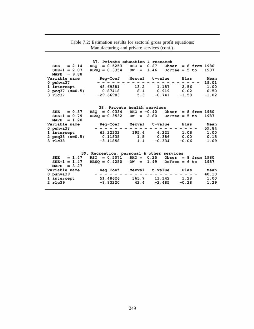
Table 7.2: Estimation results for sectoral gross profit equations:Manufacturing and private services (cont.).
37. Private education & researchSEE = 2.14 RSQ = 0.5253 RHO = 0.27 Obser = 8 from 1980SEE+1 = 2.07 RBSQ = 0.3354 DW = 1.46 DoFree = 5 to 1987MAPE = 9.88
Variable name Reg-Coef Mexval t-value Elas Mean0 pshva37 - - - - - - - - - - - - - - - - - - - - - 19.011 intercept 48.69381 13.2 1.187 2.56 1.002 pcq37 (s=0.5) 0.87418 8.1 0.919 0.02 0.503 rlc37 -29.66983 5.3 -0.741 -1.58 -1.02
38. Private health servicesSEE = 0.87 RSQ = 0.0334 RHO = -0.40 Obser = 8 from 1980SEE+1 = 0.79 RBSQ =-0.3532 DW = 2.80 DoFree = 5 to 1987MAPE = 1.20
Variable name Reg-Coef Mexval t-value Elas Mean0 pshva38 - - - - - - - - - - - - - - - - - - - - - 59.841 intercept 63.22332 195.6 6.221 1.06 1.002 pcq38 (s=0.5) 0.11835 1.5 0.386 0.00 0.153 rlc38 -3.11858 1.1 -0.334 -0.06 1.09
39. Recreation, personal & other servicesSEE = 1.47 RSQ = 0.5071 RHO = 0.25 Obser = 8 from 1980SEE+1 = 1.47 RBSQ = 0.4250 DW = 1.49 DoFree = 6 to 1987MAPE = 3.27
Variable name Reg-Coef Mexval t-value Elas Mean0 pshva39 - - - - - - - - - - - - - - - - - - - - - 40.101 intercept 51.48626 365.7 11.142 1.28 1.002 rlc39 -8.83220 42.4 -2.485 -0.28 1.29
249

Profits for Commercial and housing rents (Sector 36) and public services (sectors 40,
41 and 42) are of a different nature than the profits of manufacturing and private services.
Therefore, the above specification proved unsatisfactory for explaining profits in these
sectors. I adopted a very simple approach by regressing the nominal level of profits on
output of the respective sector inflated with the current period GDP deflator. The GDP
deflator was used to avoid the simultaneity problem of using the sector’s own price. The
results for these regressions are illustrated by Table 7.3. Finally, the national accounts data
indicate that for Domestic services (sector 43) the profits are a constant, and small (1.3
percent), proportion of value added at factor cost. Therefore, the MIDE model determines
sectoral profits with this ratio for each year.
It would be preferable to apply a more eclectic approach to estimating sectoral profits.
In particular, we would like to incorporate different explanatory factors that could reflect
market structure in different sectors or varying lags of labor and other intermediate costs.
The poor results displayed by several of the profit equations presented here attest to this fact.
However, given the limited availability of data on sectoral profits in the Spanish economy
this is not possible. Instead, I have taken an approach designed around a generic
specification in order to account for the most determinants of profit behavior: the level of
production, labor costs and international prices.
250

Table 7.3: Estimation results for sectoral gross profit equations:Commercial and residential rents and Public services.
36. Commercial and residential rentsSEE = 27.72 RSQ = 0.9928 RHO = 0.42 Obser = 8 from 1980SEE+1 = 27.41 RBSQ = 0.9916 DW = 1.15 DoFree = 6 to 1987MAPE = 1.66
Variable name Reg-Coef Mexval t-value Elas Mean0 ebe36 - - - - - - - - - - - - - - - - - - - - - 1600.091 intercept 344.15093 227.3 7.635 0.22 1.002 q36 x pgdp 0.53027 1079.4 28.784 0.78 2368.51
40. Public administrationSEE = 3.69 RSQ = 0.9831 RHO = 0.43 Obser = 8 from 1980SEE+1 = 3.65 RBSQ = 0.9803 DW = 1.15 DoFree = 6 to 1987MAPE = 3.54
Variable name Reg-Coef Mexval t-value Elas Mean0 ebe40 - - - - - - - - - - - - - - - - - - - - - 92.851 intercept 5.25947 9.1 1.068 0.06 1.002 q40 x pgdp 0.03648 668.9 18.674 0.94 2401.30
41. Public education servicesSEE = 1.44 RSQ = 0.9890 RHO = 0.15 Obser = 8 from 1980SEE+1 = 1.44 RBSQ = 0.9872 DW = 1.69 DoFree = 6 to 1987MAPE = 4.45
Variable name Reg-Coef Mexval t-value Elas Mean0 ebe41 - - - - - - - - - - - - - - - - - - - - - 33.021 intercept -6.60095 80.0 -3.665 -0.20 1.002 q41 x pgdp 0.06621 855.2 23.268 1.20 598.42
42. Public health servicesSEE = 0.39 RSQ = 0.9909 RHO = 0.34 Obser = 8 from 1980SEE+1 = 0.37 RBSQ = 0.9894 DW = 1.31 DoFree = 6 to 1987MAPE = 2.36
Variable name Reg-Coef Mexval t-value Elas Mean0 ebe42 - - - - - - - - - - - - - - - - - - - - - 14.331 intercept 2.72925 152.5 5.679 0.19 1.002 q42 x pgdp 0.01736 951.1 25.629 0.81 668.58
251

CHAPTER 8:
A FORECAST FOR THE SPANISH ECONOMY TO THE YEAR 2000:
THE IMPACT OF EUROPEAN COMMUNITY INTEGRATION
The previous chapters described the structure and equations of the MIDE model. A
principle use of the model is to provide medium to long term forecasts for up to ten years.
In this chapter, I develop an illustrative forecast of the model to the year 2000. To a large
extent, the results of a MIDE forecast depend on the values assumed for the exogenous
variables of the model. Therefore, the first section of the chapter presents and explains
several exogenous assumptions used for the forecast.
The most important influence on the Spanish economy for the next decade will be the
economic integration of the European Community. As described previously, the
specification of the MIDE model considers several factors related to the 1986 Spanish
admission to the EC. However, the greatest impacts of EC integration are yet to come. The
Europe 1992 program (beginning on January 1, 1993) will eliminate all barriers to trade,
capital and labor movements among EC countries. In order to formulate forecasts, the
model must incorporate various policy and behavioral changes implied by the European
single market program and appraise their impacts on economy. This exercise is the subject
of the second section of the chapter.
The third part of the chapter presents an outlook for the Spanish economy to the year
2000. A current debate surrounding the Spanish economy concerns whether the economy
will attain nominal convergence within the EC by the end of 1996. Under the Maastricht
treaty, convergence is necessary to allow Spain to join the common currency in 1997. It is
hoped that the forecast presented here can shed some light on the prospects for convergence.
252

8.1 Exogenous Assumptions for the Forecast to 2000
Table 8.1 displays several key assumptions used for the current forecast of the MIDE
model. For population and labor force, MIDE uses projections formulated by the Instituto
Nacional de Estadística (INE 1987). The population projection contains a steady slowdown
of growth through 2000. The labor force figures for 1992 through 1996 are based on a
recent projection supplied by the Ministry of Economics which accompanied the
"Convergence Plan" (Plan de Convergencia)1 (Cinco Dias, April 6, 1992). This forecast
corrects the original INE projection for the sharp, unexpected decline of participation rates
which occurred in 1991. By 1993 the Ministry of Economics’ figure reverts to the trend of
the INE 1987 projection. The 1997 to 2000 MIDE assumptions use the INE trend to extend
the Ministry’s 1996 projection. Table 8.1 shows a gradual decrease in labor force growth
from 1.0 percent in 1994 to 0.8 percent in 2000. This decrease is due to the ageing of the
general population and a deceleration in the growth of the female participation rate (Instituto
Nacional de Estadística 1987).
The second group of assumptions shown in Table 8.1 concerns the growth of monetary
aggregates. The forecasts for M2 and M4 assume that the authorities will target a
corresponding growth of nominal GDP. Implicit in the projections is an assumption of
progressively declining inflation from current levels. Government consumption spending,
in real terms, is borrowed from the Convergence Plan objective to keep growth to 2.0
percent per year starting in 1993. Also, the Plan projects that the government will stabilize
1 The Plan de Convergencia, put forward by the government in early April 1992, is apackage of economic policies intended to accommodate the requirements for nominalconvergence as outlined in the Maastricht treaty. Requirements for convergence and theConvergence Plan are outlined in Chapter 2. Accompanying the plan, the Ministry ofEconomics provided a forecast of macroeconomic aggregates through the year 1996. Theprojection demonstrated that nominal convergence was possible if the plan was adopted.
253

Table 8.1: Assumptions for Exogenous Variables of the MIDE Model, 1990-2000. (a)
1990 1991 1992 1993 1994 1995 1996 1997 1998 1999 2000
Demographic Projections (millions of persons):Population 38.96 39.03 39.08 39.14 39.19 39.24 39.28 39.32 39.35 39.37 39.39
percent change 0.18 0.17 0.15 0.14 0.13 0.12 0.11 0.09 0.08 0.06 0.04
Labor Force 15.02 15.07 15.16 15.32 15.47 15.61 15.75 15.89 16.02 16.15 16.28percent change 1.36 0.35 0.60 1.00 1.00 0.90 0.90 0.90 0.85 0.80 0.80
Money Supply (current prices, trillions of pesetas):M2 22.27 24.94 27.68 30.45 33.04 35.68 38.36 41.14 44.02 46.99 50.04
percent change 17.77 12.00 11.00 10.00 8.50 8.00 7.50 7.25 7.00 6.75 6.50
M4 46.38 52.41 58.17 63.99 69.43 74.98 80.60 86.45 92.50 98.74 105.16percent change 11.85 13.00 11.00 10.00 8.50 8.00 7.50 7.25 7.00 6.75 6.50
Government Spending (trillions of pesetas, 1980 prices):Consumption 3.12 3.26 3.39 3.46 3.53 3.60 3.67 3.74 3.82 3.89 3.97
percent change 4.24 4.53 4.00 2.00 2.00 2.00 2.00 2.00 2.00 2.00 2.00
Investment 1.09 1.18 1.23 1.28 1.32 1.36 1.40 1.44 1.49 1.53 1.58percent change 14.51 8.00 4.00 4.00 3.50 3.00 3.00 3.00 3.00 3.00 3.00
Exchange Rates:Pesetas/German Mark 63.09 62.56 63.00 64.00 64.50 65.00 65.00 65.00 65.00 65.00 65.00
percent change -1.43 -0.83 0.70 1.59 0.78 0.78 0.00 0.00 0.00 0.00 0.00
Pesetas/U.S. Dollar 101.93 104.30 101.43 101.76 101.26 100.75 100.75 100.75 102.70 104.00 105.30percent change -13.91 2.33 -2.75 0.33 -0.49 -0.50 0.00 0.00 1.94 1.27 1.25
Foreign Demand and Prices (1980 = 100):Foreign Demand 151.77 154.45 159.65 168.88 175.62 181.98 188.16 193.73 201.27 208.01 214.42
percent change 5.56 1.77 3.37 5.78 3.99 3.62 3.39 2.96 3.90 3.35 3.08
Foreign Prices 178.09 179.30 180.48 184.51 189.18 194.91 198.99 203.60 209.81 218.34 227.05percent change -1.16 0.68 0.66 2.23 2.53 3.03 2.09 2.32 3.05 4.06 3.99
(a) - Values for demographic, money supply, government spending, and exchange rate variables are actual for 1990-91.

investment at the current level of five percent of nominal GDP. The growth figures
displayed on Table 8.1, 4.0 percent for 1992 and 1993, 3.5 percent for 1994, and 3.0 percent
thereafter, roughly accommodate this wish in the forecast.
The exchange rates projections assume a slight depreciation of the peseta relative to
the German Mark and the other European currencies between 1992 and 1995. Presumably,
the peseta will enter the narrow band of the EC exchange rate mechanism sometime during
this period, and the government will take that opportunity to depreciate. After 1995, the
peseta should stabilize with the Mark. The peseta appreciates modestly against the U.S.
dollar through 1995, is steady in 1996 and 1997, then depreciates from 1998 to 2000.
The exogenous foreign price and demand variables for the forecast are based on an
INFORUM international modeling system scenario which simulates the effects of the
European single market (Christou and Nyhus 1992). While the following section will
describe the specific circumstances of this study, Table 8.1 summarizes its implications on
the foreign environment which will be faced by Spanish importers and exporters. The
aggregate price and demand indices shown in Table 8.1 are not strictly exogenous. They
are a weighted average of the exogenous sectoral indices, where the weights depend on the
forecasted outcomes of sectoral exports (for the demand index) and imports (for the price
index). The foreign price index is the weighted price for imports, adjusted for exchange
rates. (The projected growth rates for the competing price of exports are very similar and
their addition to the table would have added little information.) The foreign price outlook
anticipates a competitive environment brought about by the European single market. Prices
grow in the two to four percent range through 2000. Similarly, once the world economy
recovers from the doldrums of 1991 and 1992, European integration stimulates demand
increases at a brisk rate of three to four percent for the rest of the decade.
255

8.2 The Impact of the European Single Market on the Spanish Economy
Europeans have discussed the idea of creating a fully integrated European market since
the formation of the original common market of six nations in 1957.2 Integration and
expansion of the Community proceeded gradually, with fits and starts, through the following
twenty years. However, widespread economic problems caused by the oil price shocks and
high inflation of the 1970’s slowed attempts to deepen European integration. Plagued by
domestic problems of economic stagnation and high unemployment, European nations were
unable and unwilling to focus on EC issues such as trade liberalization. By the mid-80’s,
market unification was far from being realized. Eventually, however, the miserable
economic conditions and fear of Japanese and American competition prompted the EC
members to move dramatically forward.
In 1985, the European heads of state (the European Council) signed the Single European
Act. Among other items, the Act committed the EC members to the goal of "progressively
establishing the internal market over a period expiring on 31 December 1992," where "the
internal market shall comprise an area without internal frontiers in which the free movement
of goods, persons, services and capital is ensured."
The detailed measures intended to achieve the single market were outlined in a
European Commission White Paper entitled Completing the Internal Market (EC
Commission 1985). This paper identified existing barriers to the free movement of goods,
services, capital and labor between EC nations. The barriers were classified under three
categories: physical, technical and fiscal. To remove these barriers, the White Paper listed
2 The original six signatories to the initial document of the EC, the Treaty of Rome,were the Federal Republic of Germany, France, Italy, Belgium, the Netherlands andLuxembourg. Denmark, Ireland and the United Kingdom joined the EC in 1973, Greece in1981, Spain and Portugal in 1986.
256

a legislative agenda of 300 directives. The Commission’s legislative directives, often
summarized by the terms "Europe without borders", involve a large number of changes in
national law pertaining the way European economies are going to operate after 1992. In
summary, the directives mandated:
1) The removal of border controls to the physical movement of goods andpeople.
2) The removal of non-tariff barriers, especially technical standards, to themovement of goods. To accomplish this objective, the principle of"mutual recognition" will apply. This principle requires that eachmember state must accept the goods which meet the standards of anyother member.
3) The opening up of all public procurement contracts to any EC firm.
4) The deregulation of financial, business and transport services to eliminateextensive licensing and rate-setting practices which impede foreigncompetition in the domestic markets for these services.
5) The extension of the mutual recognition approach to the professions. Inother words, doctors, lawyers and other professionals who meet thelicensing requirements in any one member state can practice in anymember state.
6) Approximate harmonization of value-added and excise tax rates.
7) The elimination of all controls over capital movements within the EC.
The Europe 1992 program, as it has become known, will result in unambiguous benefits
for European consumers. The removal of barriers and regulations will result in a decrease
in consumer prices and an increase in product variety and quality. On the other hand,
producers, traditionally operating in smaller, often protected, markets, will face stiff new
competition. Many firms will suffer short-run profit losses and others will find their
viability threatened. Successful firms will take advantage of new market opportunities and
benefit from expansion of real incomes brought about by the program. Increased
257

competition will induce firms to adjust their behavior and exploit economies of scale in
production, reduce X-inefficiencies3 and internalize externalities in learning and innovation.
At the macroeconomic level, reductions in production costs and increases in productivity
growth will result in greater price stability. Therefore, the long-run competiveness of
European firms, vis-á-vis the rest of the world, will increase. Greater export activity, the
expansion in consumer real income and price stability will stimulate investment. This
virtuous circle should eventually reduce Europe’s long-standing unemployment problems.
Since the Single European Act, the pending completion of the internal market has
dominated economic discussion in Europe. A large number of studies estimate the potential
effects of the integration. The best known study was undertaken by the Commission of the
European Communities, the so-called Cecchini Report (Cecchini et al. 1988). This report
was the summary of a large research effort, occupying two volumes of EC Commission
studies, which investigated and quantified both the potential microeconomic and
macroeconomic consequences of European market integration. Table 8.2 displays a
summary of the benefits of the single market estimated by this research. The table illustrates
the Cecchini Report’s conclusion that the benefits of removing trade barriers in the EC are
enormous, estimating potential gains from the single market to be as high as Ecu 216 billion
($270 billion) (Cecchini et al. 1988, Table 9.2).
Alternative estimates reach more subdued appraisals of the benefits of the integrated
market. While the Cecchini Report projects a gain of 3.2 to 5.7 percent for total Community
GDP, other studies report a gain of only 1.5 to 2.5 percent (Peck 1989). On the other hand,
3 One often encounters the term "X-inefficiencies" in discussions concerning ECintegration. This term refers to management inefficiencies promoted by a non-competitiveenvironment which lead, for example, to excessive administrative overhead costs, over-manning at all levels, or the inefficient management of inventories.
258
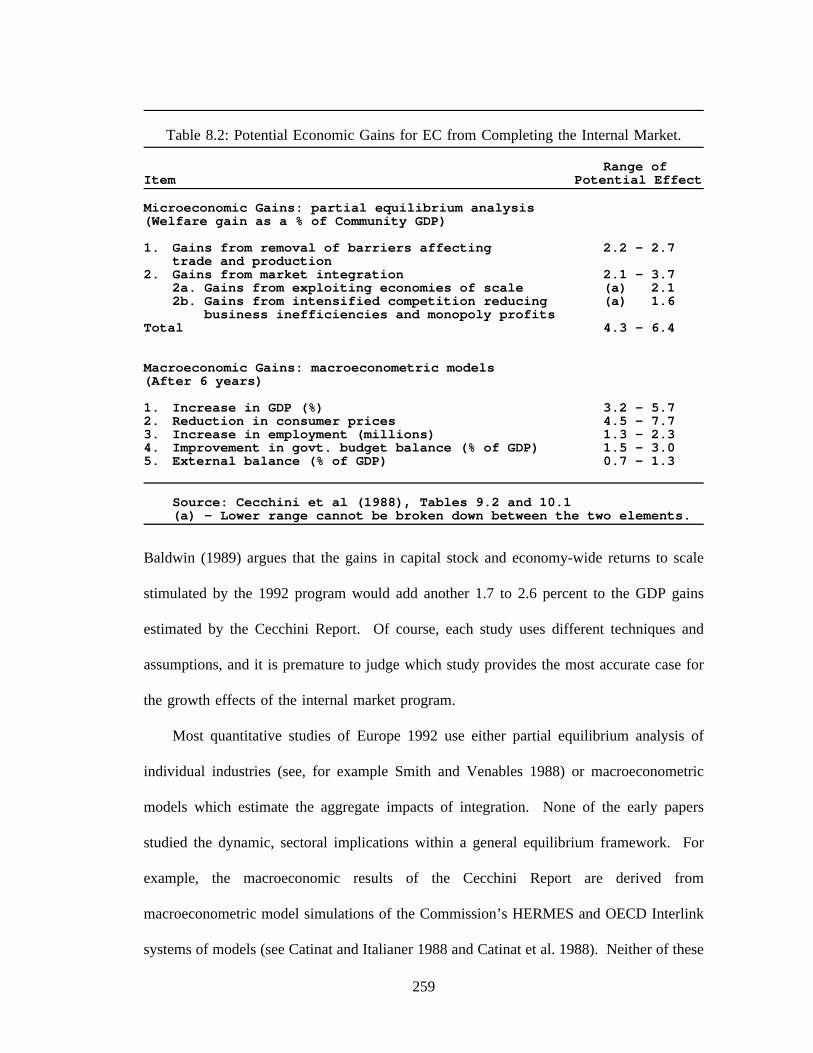
Table 8.2: Potential Economic Gains for EC from Completing the Internal Market.
Range ofItem Potential Effect
Microeconomic Gains: partial equilibrium analysis(Welfare gain as a % of Community GDP)
1. Gains from removal of barriers affecting 2.2 - 2.7trade and production
2. Gains from market integration 2.1 - 3.72a. Gains from exploiting economies of scale (a) 2.12b. Gains from intensified competition reducing (a) 1.6
business inefficiencies and monopoly profitsTotal 4.3 - 6.4
Macroeconomic Gains: macroeconometric models(After 6 years)
1. Increase in GDP (%) 3.2 - 5.72. Reduction in consumer prices 4.5 - 7.73. Increase in employment (millions) 1.3 - 2.34. Improvement in govt. budget balance (% of GDP) 1.5 - 3.05. External balance (% of GDP) 0.7 - 1.3
Source: Cecchini et al (1988), Tables 9.2 and 10.1(a) - Lower range cannot be broken down between the two elements.
Baldwin (1989) argues that the gains in capital stock and economy-wide returns to scale
stimulated by the 1992 program would add another 1.7 to 2.6 percent to the GDP gains
estimated by the Cecchini Report. Of course, each study uses different techniques and
assumptions, and it is premature to judge which study provides the most accurate case for
the growth effects of the internal market program.
Most quantitative studies of Europe 1992 use either partial equilibrium analysis of
individual industries (see, for example Smith and Venables 1988) or macroeconometric
models which estimate the aggregate impacts of integration. None of the early papers
studied the dynamic, sectoral implications within a general equilibrium framework. For
example, the macroeconomic results of the Cecchini Report are derived from
macroeconometric model simulations of the Commission’s HERMES and OECD Interlink
systems of models (see Catinat and Italianer 1988 and Catinat et al. 1988). Neither of these
259

systems contain models with substantial disaggregation. This deficiency has been remedied
by the work of Christou and Nyhus (1992 - also referred to below as CN). Their objective
was to shed some additional light to the potential effects of Europe 1992 by means of a the
INFORUM trade-linked system of macroeconomic, multisectoral models.
The CN study of the Europe 1992 program applied to only four of the twelve European
Community countries: Germany, France, Italy and Belgium.4 Therefore, the results of the
study exhibit a relative downward bias. The lack of feed-back effects from the other
European economies limits the favorable results expected by the integration. Nevertheless,
according to the CN results, the integration process will boost the European economies
substantially. CN conclude that, by 1998, the Europe 1992 program will increase GDP by
5.35 percent in Belgium, 4.84 percent in France, 4.99 percent in Germany and 3.47 percent
in Italy (pp. 17-20).5 The corresponding percentage increases in exports will be 9.46, 8.68,
6.28 and 4.27. Also by 1998, the integration programs boosts employment by 0.81 percent
in Belgium, .60 percent in France, and 0.23 percent in Germany. For Italy, however, the
number of jobs eliminated by higher rates of productivity growth is greater than those
created by demand expansion. Therefore, employment is lower by 1.28 percent.
Beyond Germany, France, Italy and the United Kingdom, all the studies, including that
of Catinat et al. (1988 - referred to below as simply Catinat), have very little to say about
4 At the time of the CN study, the MIDE model was part of the system, but not fullyoperational. While it was included in the inter-linked projections of the system, the modeldid not incorporate the Europe 1992 shocks. Also, the model of Belgium does not have aprice side, and, thus, it does not produce forecasts for prices.
5 CN present figures up to the year 2010. I chose the year 1998 in this case, becauseit corresponds to the six year horizon used by Catinat et al. (1988). The increases in GDPcomputed in that study were 4.20 percent for Germany, 5.05 percent for France and 5.46percent for Italy and 4.00 percent for the United Kingdom (pp. 621-22). Complete resultsfor Belgium were not available.
260

the impact of integration on the Spanish economy. For instance, Spain is included in only
one of the four macroeconomic simulations (financial liberalization) used by Catinat for
estimating the impacts of various single market measures. Only Polo and Sancho (1989)
have attempted a specific study of the integration effects of 1992 for the Spanish economy,
and their study is a strictly comparative static exercise.
This section provides a dynamic assessment, both at the macroeconomic and industry
level, of the impacts of the single market program on the Spanish economy. The initial
stage of the work consisted of the development of a base forecast of the MIDE model that
assumes that Spain does not implement the EC directives for the 1993-2000 period. This
base scenario, which is labelled Spain with Borders, does assume that the Spain fulfills its
original EC agreements with respect to the reduction to zero of all intra-EC tariff rates.
Also, in order to eliminate the need to run full INFORUM system simulations, the
exogenous foreign demand and competing price of export variables used for the base case
are derived from the CN simulation of Europe without Borders. In other words, the base
scenario assumes that the rest of the EC goes happily along with the internal market
program, but that Spain does not.
The next stage of the analysis formulates various modifications to the base scenario
which correspond to the implementation of the various Europe 1992 directives. Drawing
upon the work of Catinat and Christou and Nyhus, a number of assumptions were made,
quantified and introduced into the MIDE model. The changes to the model can be regarded
as a sequence of major exogenous price and supply-side shocks which simulate the effects
of market integration. There are five scenarios; each one corresponds to a different,
separable aspect of the single market program. The scenarios address:
261

1) The elimination of customs controls over flows of goods.
2) The opening of domestic public procurement to all EC firms.
3) The liberalization of financial services.
4) The supply effects of firm’s strategic reactions when faced with thechange in competitive environment as a result of the internal market.
5) The harmonization of value added and excise taxes.
The first four alternatives are the same as those distinguished in the Catinat and CN
studies. A fifth scenario for fiscal harmonization is added because present Spanish value
added and excise tax rates for certain goods are substantially different than the EC average.
While the fiscal harmonization aspect of the single market program has been pushed ahead
by two to three years, presumably the Spanish government will have to revise several tax
rates by 1995 or 1996. Finally, a sixth scenario is presented where all of the shocks are
loaded into the model to quantify the impact of the entire single market program on the
Spanish economy. This scenario, called Spain in the Single Market, is also the forecast for
the Spanish economy presented in the next section of this chapter.
The application of each of the shocks in the model is conservative in that the full effects
are spread over eight years (1993-2000). This is done for two reasons. First, the
simulations describe the impacts of phenomena identified in various studies as logical
outcomes of market integration. However, it is difficult to know how long it will require
for these phenomena, such as a greater exploitation of economies of scale, to manifest
themselves fully. Therefore, a conservative approach is warranted. Second, the insertion
of the shocks into the model assumes that the EC member governments, and especially the
Spanish government, adopt all of the directives mandated by the program. However, it is
262

probable that foot-dragging among member governments will delay the full implementation
of various measures.
The scenarios do not consider other implications of the single market which are difficult
to quantify. Most important are the dynamic effects identified by Baldwin (1989), among
others, which could substantially increase the potential growth of the EC economies.
Examples include the competition effects on innovation and a change in the long-run
productivity growth rate generated by a more favorable savings and investment climate. For
example, since sectoral productivity growth is essentially exogenous in the MIDE model,
it cannot endogenously predict enhancements to the potential output of the economy which
may be brought about by greater levels of investment stimulated by EC integration. Thus,
the model does not provide a solution to Dornbusch’s recent lament that:
"The margin of error (of studies assessing the quantitative impacts of ECintegration) is large simply because there are no available models with which toevaluate multicountry, multisectoral supply-side economics both in terms of long-run growth and short-run macroeconomics (1989, p. 348-9).
Nevertheless, the scenarios do contribute a useful estimation for predicting the relative
impacts of the various aspects of the Europe 1992 program on the Spanish economy.
Moreover, despite the identified shortcomings, the model does provide practical information
for evaluating the prospects waiting, and for identifying possible problems confronting, the
Spanish economy.
263

The Elimination of Customs Controls
Imagine a truck driver hauling a consignment of goods from Chicago to Washington,
D.C., a distance of approximately 600 miles, or 12 hours. Suppose that for each of the five
state border crossings required by this journey, the driver had to stop and satisfy customs
formalities for each individual state. Moreover, each crossing requires a different set of
paperwork and could entail a delay of anywhere from 20 minutes to 2 hours. It is easy for
one to imagine that such a situation would add substantially to the transport cost of the
consignment. This is precisely the situation in the EC today.
Despite the fact that there is no tariffs or quota restrictions on trade between the fully-
integrated EC nations, the costs associated with border controls and customs formalities
continues to hamper trade among the members. A number of the single market directives
mandate the elimination of all border controls and the reduction and standardization of
administrative formalities by the end of 1992. Implementation of the measures will reduce
two types of costs. First, government employment will be reduced by the number of
customs officers made redundant by the measures. This cost reduction was implemented in
the MIDE model by reducing public employment by 8000 jobs at the beginning of 1993.
The second cost reduction will be in the price of the intra-Community trade, since the
costs of border delays and administrative formalities are paid either directly or indirectly by
importing firms. Catinat and Italianer (1988) estimated the proportion of the cost of the
administrative formalities in the total value of the bilateral trade flows for several EC
countries. The shares, displayed in Table 8.3, are based on estimates of the administrative
costs for per consignment, for both exporters and importers, and for different products. The
entries the Table 8.3 represent the proportion of the prices which can be attributed to
customs delays and formalities, for exports from the row country to the column country.
264

Table 8.3: Share of the Cost of the Administrative Formalities Borne by Firmsin the Value of Bilateral Trade Flows - All Products Taken Together (percent).
Importer: Belgium Germany France Italy Nethlnds UK Oth. ECExporter
Belgium . 0.84 1.21 1.42 0.94 0.84 1.01Germany 1.45 . 2.10 2.17 1.82 1.67 1.85France 1.64 1.72 . 2.25 1.84 1.72 1.69Italy 1.76 2.25 2.30 . 1.95 1.83 1.80Netherlands 1.05 1.22 1.40 1.59 . 1.27 1.35UK 1.87 1.20 1.55 1.91 1.33 . 1.76Oth. EC 1.49 2.02 2.10 2.14 1.73 1.79 1.82
Source: Catinat and Italianer (1988).
To simulate the elimination of these costs in bilateral trade, Christou and Nyhus
assumed that the elimination of customs controls would result in a reduction of each
country’s sectoral export prices. To compute the appropriate sectoral export price reductions
for each country, they combined the destination shares of each country’s exports with the
information of Table 8.3. For any given exporting country, define si,k as the share of that
country’s exports of sector i to country k in the total value of the country’s exports to
country k. Then, define the price reduction factors for exports to country k, RFk, to be the
appropriate values across the row of Table 8.3 for the exporting country. The sectoral
export prices are then reduced with weighted-average reduction factors (WARFi) calculated
according to the formula:
WARFik
(si,k ×RFk )
where Σi si,k = 1 for all k. Sectoral export prices for each exporting country are reduced by
the weighted reduction factors starting in 1993.
The Spain with Borders base case assumes that since Spain did not adopt the single
market program, border controls to Spanish exports in the rest of Europe remained. To
265
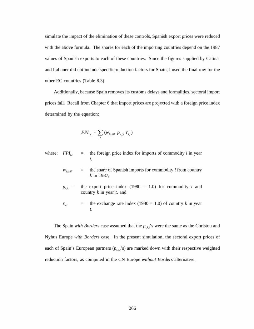
simulate the impact of the elimination of these controls, Spanish export prices were reduced
with the above formula. The shares for each of the importing countries depend on the 1987
values of Spanish exports to each of these countries. Since the figures supplied by Catinat
and Italianer did not include specific reduction factors for Spain, I used the final row for the
other EC countries (Table 8.3).
Additionally, because Spain removes its customs delays and formalities, sectoral import
prices fall. Recall from Chapter 6 that import prices are projected with a foreign price index
determined by the equation:
FPIi,tk
(wi,k,87 pk,i,t rk,t )
where: FPIi,t = the foreign price index for imports of commodity i in yeart,
wi,k,87 = the share of Spanish imports for commodity i from countryk in 1987,
pi,k,t = the export price index (1980 = 1.0) for commodity i andcountry k in year t, and
rk,t = the exchange rate index (1980 = 1.0) of country k in yeart.
The Spain with Borders case assumed that the pi,k,t’s were the same as the Christou and
Nyhus Europe with Borders case. In the present simulation, the sectoral export prices of
each of Spain’s European partners (pi,k,t’s) are marked down with their respective weighted
reduction factors, as computed in the CN Europe without Borders alternative.
266

Table 8.4: Elimination of Border Controls - Comparison to Spain With Borders Case.(1980 prices, except where otherwise indicated.)
1993 1994 1995 1996 1997 1998 1999 2000Percentage deviations
Gross domestic product 0.06 0.22 0.26 0.23 0.24 0.26 0.29 0.32Private national consumption 0.15 0.48 0.47 0.34 0.56 0.76 0.85 0.82Fixed capital investment 0.12 0.46 0.52 0.41 0.41 0.41 0.52 0.53Exports 0.45 1.03 1.21 1.27 1.40 1.60 1.83 1.77Imports 0.53 1.38 1.41 1.28 1.74 2.14 2.41 2.20
GDP deflator -0.47 -0.32 -0.12 -0.40 -0.41 -0.45 -0.52 -0.35Private consumption deflator -0.52 -0.50 -0.42 -0.65 -0.74 -0.94 -1.06 -0.81Fixed investment deflator -0.63 -0.56 -0.50 -0.69 -0.73 -1.14 -1.18 -0.90Export deflator -1.27 -1.25 -1.21 -1.34 -1.45 -1.79 -1.85 -1.54Import deflator -1.48 -1.83 -1.64 -1.62 -2.37 -3.28 -3.28 -2.41
Real disp. income per capita 0.16 0.45 0.57 0.49 0.65 0.82 0.92 0.84Aggregate labor productivity 0.06 0.06 0.06 0.11 0.06 0.06 0.11 0.11Real wage rate 0.20 -0.05 -0.05 0.21 0.19 0.14 0.16 0.15Employment 0.00 0.16 0.18 0.14 0.18 0.19 0.20 0.20
Absolute deviations
Current account deficit -0.03 -0.06 -0.05 -0.05 -0.13 -0.20 -0.19 -0.08(% of GDP, current prices)Government deficit -0.05 -0.17 -0.22 -0.20 -0.27 -0.35 -0.41 -0.43(% of GDP, current prices)Employment (thousands) 0.09 20.34 23.76 17.99 23.86 25.69 27.02 27.83Unemployment rate (%) -0.00 -0.13 -0.15 -0.11 -0.15 -0.16 -0.17 -0.17Long term interest rate (%) -0.38 -0.24 0.09 -0.18 -0.33 -0.35 -0.38 -0.09
The results of removing the border restrictions, as simulated by the MIDE model, are
shown in Table 8.4. The first part of the table presents the deviations for macroeconomic
variables as a percent of the figure generated under the Spain with Borders alternative. The
second part of the table displays the absolute deviations for various indicators. All of the
macroeconomic variables are improved in the scenario. By 1998, the GDP expands by .26
percent, the GDP deflator decreases by .45 percent, and the consumption price declines by
.94 percent.6 Employment increases by more than 25 thousand jobs. The combination of
lower relative import prices and increases in real income lead to real import growth that
6 While projections in the tables extend to the year 2000, in general, figures quoted inthe text will be for 1998 to facilitate comparisons with the Cecchini report. It defines a six-year "medium-term" horizon (Catinat et al. 1988). Another consideration is that deviationsfrom the base run tend to grow sharply in 1999 and 2000. Therefore, the 1998 figurespresent a preferable summary, since they better reflect the tendencies in the earlier years.
267

exceeds export growth. Despite this deterioration of the real trade balance, a more favorable
terms of trade position (export prices over import prices) improves the nominal current
account deficit by .20 percent of GDP in 1998. Stronger growth also bodes well for the
government deficit, which declines by .35 percent of GDP by 1998. The conclusion one
could make from this story is that a good dose of free trade will be beneficial to the Spanish
economy.
Opening of Public Procurement to Foreign Suppliers
In 1986, public-sector contractual procurement was estimated to be 7 to 10 percent of
European Community GDP (Cecchini 1988, p.16). Currently, only a tiny fraction of these
purchases are awarded to non-national suppliers. This entrenched protectionism is rarely
codified by law, but it is sustained by official and un-official policy. Not only does the
protection extend to goods bought by the public administration, health and defense sectors,
but also to the telecommunications, transportation and energy industries dominated by
government enterprises.
The costs produced by sealed procurement markets are major and various. The most
obvious cost is that government agencies and public enterprises pay more for equipment
goods and infrastructure projects than they would under open competition. Additionally,
private market prices are inflated because of the dominant market positions held by national
champions, positions which might be unsustainable without guaranteed public procurement
contracts. Finally, the non-competitive environment stifles incentives for attaining greater
efficiency and innovation in the protected industries.
268

The single market program aims to end these practices by mandating that national
procurement rules be applied equally to all firms located in EC member countries. The
Cecchini Report identifies three effects of these measures (p. 17):
1) A "static trade effect" where public authorities will be buying from thecheapest supplier. This will lead to import penetration for the relevant supplysectors and a reduction in the price inflation of publically supplied services.
2) A dynamic "competition effect" leading to a downward pressure on prices asthe domestic firms in the previously protected industries attempt to competewith the foreign entrants.
3) A dynamic "restructuring effect," where domestic firms in the affectedindustries reorganize under the competitive conditions. Cost savings will berealized from the exploitation of economies of scale and the reduction of X-inefficiencies and monopoly profits.
In order to simulate these effects in the HERMES national models, Catinat et al. (1988,
p. 379) used quantitative information supplied by WS Atkins Management Consultants
(1988). This study was sponsored by the EC Commission to assess the microeconomic
implications of open public procurement. With this information, Catinat estimated import
penetration and price shocks for insertion into each of the country models (Table 8.5). The
shocks were applied to the investment goods industries according to the proportion of public
sector purchases from the industry. The scenario assumed that all enterprises in the
transport, telecommunications and energy sectors were public enterprises.
The figures of Table 8.5 were used to introduce similar shocks into the MIDE model.7
Specific shocks were not available for Spain. One option was to use the average value of
7 Open public procurement will also apply to public sector purchases of intermediategoods. However, examinations of the import coefficients of several Spanish input-outputtables did not reveal any marked pattern of discrimination against imports for intermediateconsumption. Therefore, the current scenario concerns public procurement for investmentonly.
269

Table 8.5: Shocks Introduced into the HERMES Model forOpening up of Public Procurement.
Belgium Germany France Italy UK
Static Effects 8.2 8.5 5.5 4.1 3.6Increase in level ofimport penetration inpublic markets (%)
Competition & Restructuring EffectsFall in prices of equipmentgoods on public markets (%)- public administration 0.03 0.13 0.03 0.07 0.12- public enterprises
* energy 1.6 1.5 1.7 1.1 1.1* transport and telecom 8.5 7.8 7.6 11.4 7.2
- public health and education (a)
Source: Catinat et al. (1988).(a) - Price reductions for these sectors were not identified by Catinat et
al. A 10 percent reduction was assumed.
the shocks provided in Table 8.5. However, since closed government procurement is
especially pervasive in Spain, I chose, instead to use the largest shock from each row of
Table 8.5 (underlined values). Also, I assumed a competition and restructuring price
reduction factor of 10 percent for the investment purchases of the public education and
health sectors (not distinguished by Catinat). To facilitate the following explanation of the
implementation of the shocks, the capital goods industries and the public sectors of the
MIDE model effected by the direct impacts of the shocks are displayed in Table 8.6.
The import penetration shock increases the imports for the capital goods industries
(there are no construction imports) which are otherwise estimated in the model. The amount
of the increase is computed in the model by the formula:
δIMPi,tj
(bi,j × INVi,t × PFt )
where: δIMPi,t = increase in the imports which were predicted by theequations of the model for capital goods industry i (seeTable 8.6) for time t,
bi,j = the share of investment purchases from industry i boughtby public sector j (see Table 8.6),
270

Table 8.6: MIDE Model Sectors Effected by the Direct Impactsof the Open Public Procurement Simulation.
Capital goods suppliers (i sectors):9. Metal products, except machinery and transport10. Industrial and agricultural machinery11. Office machinery, computers, prec. instruments12. Electrical and electronic material and accessories13. Motor vehicles and engines14. Other transport material26. Construction and civil engineering
Public Administration and Enterprises (j sectors):
Energy2. Coal, lignite, and radioactive material3. Coke products4. Crude petroleum, natural gas and refining5. Electrical, gas, steam and water utilities
Transport and Communications30. Interior transport (not including highway transportation)31. Maritime and air transport (not including air transport)32. Transport services33. Communications
Public Services40. Public administration41. Public education services42. Public health services
INVi,t = total investment sales of capital goods industry i, and
PFt = the import penetration factor.
The bi,j coefficients, which are constant through time, come from Antón and Escribano
(1988) and are identical to those used for the computation of the investment demand indices
of the investment equations (see Chapter 5). The import penetration factor increases linearly
from .011 in 1993 until it reaches its maximum value of .085 (the German figure from Table
8.5) in 2000. This lagged realization of the shock reflects an assumption that foreign firms
will only gradually attain market share in public procurement.
The dynamic competitive and restructuring price reductions for the capital goods
industries result from the elimination of monopoly rents and improvements in labor
productivity. The price decreases are implemented in the model through gradual reductions
271

in gross profits and improvements in productivity. To insure that the reductions in labor
requirements implied by the productivity shocks result in equivalent decreases in labor costs,
the exogenous productivity shocks are not permitted to feed back into the wage rate.8 The
profit and wage decreases are computed with the formula:
δVAi,tj
(bi,j × PRFj,t )
where: δVAi,t = decrease in the profits and wages which were predicted bythe equations of the model for capital goods industry i fortime t,
bi,j = the share of investment purchases from industry i boughtby public sector j, and
PRFj,t = the price reduction factor for public procurement sector j.
The price reduction coefficients increase linearly from one eighth of their total value
indicated in Table 8.5 to the full impact in 2000.
Reductions in procurement supply prices are complemented with direct reductions in
the prices of public enterprise production and public services. Since, investment purchases
are paid from gross profits, through retained earnings and interest payments, expenditure
savings for public procurement are deducted from the gross profits of the purchasing sectors.
The expenditure savings are realized in the MIDE model by the formula:
8 Recall from Chapter 7 that sectoral level wage rates depend on labor productivity.Allowing the exogenous productivity shocks to feed back into the wage rate through thewage equations would result in much of the productivity gain accruing to labor. Since theobject of this exercise is to decrease the costs of production, a compensating negative shockis applied to total wages so that the employment reducing effects of productivity increasestranslates into an equal decrease in wages. This assumption does not mean that the sectoralwage rate is the same as in the base scenario. Endogenous increases in the wage rates arepermitted. For example, cyclical increases in productivity will increase the rate through thewage equations in the normal way.
272

δPROFj,ti
(bi,j × INVi,t × PVi,t × PRFj,t)
where: δPROFj,t = decrease in gross profits otherwise predicted by theequations of the model for public sector j,
bi,j = the share of investment purchases from industry ibought by public sector j,
INVi,t = total investment sales of capital goods industry i,
PVi,t = the price of capital goods sold by industry i.
PRFj,t = the price reduction factor for public procurementsector j.
Reductions in gross profits, in turn, lead to reductions in producer prices for the public
sectors through the input-output price equation.
The scenario results appear in Table 8.7. The general price level is down significantly,
registering decreases of 1.7 percent for the GDP deflator and 1.4 percent for the
consumption deflator by 1998. The lower prices stimulate domestic demand and exports,
but the higher growth is not significant until 1995-96. In fact, the initial impact of
restructuring results in a net loss of jobs in 1993. Throughout the forecast horizon, jobs are
lost in the capital goods industries and, until 1996, in construction. Since these are relatively
high paid positions, the short-run loss in tax revenues offsets the government savings in
purchasing, resulting in a larger budget deficit through 1994. The most notable effects occur
in the production prices of the public enterprise sectors. Table 8.7 reports significant price
reductions for energy and transport, and especially, communications. These price decreases
account for the large decline in the consumption price deflator. Ironically, the opening of
public procurement may bring the greatest benefit to Spanish consumers.
273

Table 8.7: Opening of Public Procurement - Comparison to Spain With Borders Case.(1980 prices, except where otherwise indicated.)
1993 1994 1995 1996 1997 1998 1999 2000
Percentage deviations
Gross domestic product 0.01 0.08 0.20 0.33 0.48 0.65 0.83 1.02Private national consumption 0.01 0.11 0.23 0.33 0.48 0.62 0.75 0.93Fixed capital investment 0.02 0.16 0.35 0.55 0.76 0.94 1.10 1.28Exports 0.07 0.21 0.36 0.54 0.76 0.96 1.20 1.45Imports 0.06 0.24 0.41 0.54 0.71 0.77 0.83 0.99
GDP deflator -0.27 -0.45 -0.70 -1.01 -1.35 -1.70 -2.09 -2.59Private consumption deflator -0.17 -0.37 -0.55 -0.80 -1.10 -1.37 -1.69 -2.04Govt. consumption deflator -0.15 -0.34 -0.53 -0.75 -0.95 -1.22 -1.47 -1.82Fixed investment deflator -0.24 -0.38 -0.58 -0.83 -1.06 -1.37 -1.64 -1.97Export deflator -0.24 -0.39 -0.56 -0.77 -1.01 -1.27 -1.54 -1.84Import deflator 0.01 0.04 0.06 0.08 0.10 0.12 0.13 0.14
Real disp. income per capita -0.07 -0.03 0.04 0.13 0.23 0.29 0.38 0.48Aggregate labor productivity 0.06 0.12 0.11 0.17 0.17 0.22 0.27 0.27Real wage rate 0.14 0.12 0.20 0.31 0.42 0.52 0.66 0.90Employment -0.03 0.01 0.09 0.18 0.31 0.44 0.58 0.73
Absolute deviations
Current account deficit 0.07 0.11 0.16 0.21 0.26 0.32 0.36 0.38(% of GDP, current prices)Government deficit 0.02 0.02 -0.01 -0.04 -0.08 -0.12 -0.16 -0.22(% of GDP, current prices)Employment (thousands) -3.52 1.15 11.54 24.46 41.03 59.99 79.73 102.28Unemployment rate (%) 0.02 -0.01 -0.07 -0.15 -0.26 -0.38 -0.49 -0.63Long term interest rate (%) -0.13 -0.23 -0.22 -0.28 -0.35 -0.40 -0.50 -0.64
Employment in the capital goods industries:Absolute deviation in thousands
9. Metal products -1.12 -2.10 -2.93 -3.70 -4.45 -5.16 -5.86 -6.5110. Industrial machinery -0.56 -1.24 -1.90 -2.59 -3.25 -3.93 -4.63 -5.3411. Office mach. & computers -0.06 -0.13 -0.16 -0.16 -0.15 -0.15 -0.15 -0.1412. Elect. mach. & material -1.11 -1.57 -2.02 -2.51 -2.94 -2.82 -1.80 -1.3513. Motor vehicles & engines -0.42 -0.56 -0.73 -1.00 -1.12 -1.24 -1.39 -1.4414. Other transport equip. -0.38 -0.76 -1.07 -1.31 -1.41 -1.61 -1.80 -1.9726. Construction -1.09 -1.74 -1.44 -0.47 0.73 1.81 2.76 3.69
Public administration and enterprise production pricesPercentage deviation
2. Coal and lignite -0.19 -0.49 -0.84 -1.22 -1.56 -1.95 -2.36 -2.913. Coke products -0.31 -0.58 -0.90 -1.32 -1.69 -2.08 -2.53 -3.094. Petrol. products -0.19 -0.30 -0.40 -0.55 -0.79 -1.00 -1.14 -1.325. Electric & water util. -0.46 -0.64 -0.97 -1.41 -1.95 -2.47 -3.11 -3.8130. Interior transport -0.17 -0.28 -0.45 -0.72 -0.93 -1.22 -1.54 -1.7631. Maritime & air transport -0.32 -0.57 -0.88 -1.24 -1.60 -1.96 -2.37 -2.8032. Oth. transport services -0.34 -0.58 -0.89 -1.25 -1.68 -2.09 -2.47 -2.7933. Communications -0.82 -1.63 -2.46 -3.30 -4.11 -5.02 -5.92 -6.8040. Public administration -0.11 -0.29 -0.45 -0.63 -0.82 -1.02 -1.25 -1.5441. Public education -0.22 -0.50 -0.76 -1.06 -1.40 -1.71 -2.06 -2.5242. Public health services -0.18 -0.38 -0.59 -0.81 -1.06 -1.32 -1.60 -1.96
274

Deregulation of Financial Services
Financial market regulation is pervasive in EC countries. Standards and controls have
restricted market entry in many financial sectors, abolishing free competition. As a result,
there are large differences in the prices of standard financial products across the EC. Price
differentials between nations range from 46 percent for obtaining travellers cheques to 254
percent for insurance against commercial fire and theft (Cecchini 1988, Table 6.1).
Commission directives for the deregulation of financial services envisions the elimination
of regulations discriminating against foreign entities in the domestic market and a gradual
harmonization of regulations. Most of the EC nations, Spain included, have started to move
toward this ideal. By 1993 the large majority of regulations restricting foreign entry into
the Spanish financial markets should be swept away.
The increased competition in financial services brought about by deregulation will result
in lower profit margins and increased productivity for the domestic industries. Gradually,
domestic prices for these services will converge with the EC average. The Cecchini
Report’s (Table 6.2) mid-range estimates of potential price reductions in financial services
are 11 percent for Belgium, 12 percent for France, 10 percent for Germany, 14 percent for
Italy and 7 percent for the United Kingdom. The corresponding figure for Spain is a
whopping 21 percent. For the MIDE model simulation, I gradually introduce this 21 percent
price reduction over the course of 1993-2000 (Table 8.8). Half of the decrease in the price
is administrated through an increase in labor productivity compensated, as discussed for the
public procurement scenario, with an equivalent wage shock. The other half of the price
reduction comes through a reduction in profits. Table 8.8 reports that the impact on the
economy is dramatic.
275

Table 8.8: Financial Liberalization - Comparison to Spain With Borders Case.(1980 prices, except where otherwise indicated.)
1993 1994 1995 1996 1997 1998 1999 2000
Percentage deviations
Price of financial services -2.09 -4.32 -6.75 -9.21 -11.89 -14.56 -17.42 -20.44
Gross domestic product 0.04 0.15 0.38 0.73 1.17 1.73 2.38 3.20Private national consumption 0.04 0.14 0.36 0.66 1.02 1.54 2.06 2.75Fixed capital investment 0.03 0.16 0.44 0.86 1.37 1.99 2.63 3.38Exports 0.04 0.18 0.40 0.71 1.17 1.72 2.39 3.16Imports 0.01 0.08 0.23 0.48 0.68 0.98 1.17 1.42
GDP deflator -0.13 -0.45 -0.91 -1.53 -2.45 -3.43 -4.73 -6.36Private consumption deflator -0.14 -0.44 -0.80 -1.30 -2.05 -2.79 -3.88 -5.14Fixed investment deflator -0.16 -0.41 -0.76 -1.25 -1.86 -2.57 -3.46 -4.60Export deflator -0.17 -0.44 -0.79 -1.22 -1.83 -2.47 -3.35 -4.46Import deflator 0.00 0.01 0.03 0.04 0.06 0.09 0.11 0.13
Real disp. income per capita 0.06 0.14 0.27 0.49 0.77 1.08 1.46 1.78Aggregate labor productivity 0.06 0.12 0.17 0.28 0.34 0.33 0.44 0.54Real wage rate -0.06 -0.16 -0.28 -0.40 -0.41 -0.50 -0.46 -0.38Employment -0.01 0.04 0.20 0.47 0.85 1.35 1.93 2.65
Absolute deviations
Current account deficit 0.03 0.08 0.15 0.24 0.35 0.48 0.61 0.73(% of GDP, current prices)Government deficit -0.00 -0.01 -0.06 -0.15 -0.27 -0.43 -0.61 -0.80(% of GDP, current prices)Employment (thousands) -1.74 5.06 26.15 62.73 113.80 184.09 265.75 369.29Unemployment rate (%) 0.01 -0.03 -0.17 -0.40 -0.72 -1.15 -1.64 -2.27Long term interest rate (%) -0.05 -0.21 -0.36 -0.50 -0.78 -0.98 -1.33 -1.91
In 1988, the value added of financial services accounted for approximately 6.5 percent
of the GDP in the Spanish economy. The consumer budget share for financial services
hovers around .5 percent. A large reduction in the costs of these services, then, would have
an important direct impact on price inflation in the economy. More important, however, is
that virtually every industry of the economy purchases a non-trivial amount of intermediate
financial services (margins on loans, for instance). Therefore, a 20 percent price reduction
in financial services stimulates a huge indirect reduction of price inflation for all other goods
and services. This indirect price effect contributes to a 3.4 percent reduction in the GDP
deflator by the year 1998. The reduction in prices stimulates increase in exports and real
incomes which translate into a 1.7 percent increase in real GDP. Also notably, is the that
276

fixed investment is up 2.0 percent by 1998. The only bad news is on the foreign account.
Greater domestic growth and a deterioration in the terms of trade causes the current account
deficit to increase by .43 percent of GDP. The results leave little doubt that, of all the
Europe 1992 measures, the deregulation of financial services will have the greatest impact
of on the Spanish economy.
Supply Effects
The generic term "supply effects" refers to changes in producer behavior which will be
prompted by the integration of the single European market. The single market will boost
competition, reducing monopoly rents and management inefficiencies (X-inefficiencies).
Moreover, the abolition of technical standards and other non-tariff barriers places EC firms
in a market the size of the entire community. A larger, homogeneous market will provide
the opportunity to exploit economies of scale in production, marketing and distribution.
Whatever the nature of the supply effects, they will be manifested by falling costs of
production.
Much of the impact of competition-induced improvements in management efficiency
and the reduction of monopoly rents will occur as a reduction of profits, the rest as
decreases in wage costs. Reductions in wage costs are implemented in the model as labor
productivity increases, where, once again, the exogenous productivity shock is not permitted
to feed back into the wage rate. Therefore, reductions in labor requirements result in equal
reductions in labor costs. The magnitude of the shocks are displayed in Table 8.9. The
figures were adapted from Catinat et al. (1988), who derived them by using the differences
in prices now observed between member states as an indicator of future competitive
pressures. The magnitude of the cost reductions vary according to the type of industry. The
277
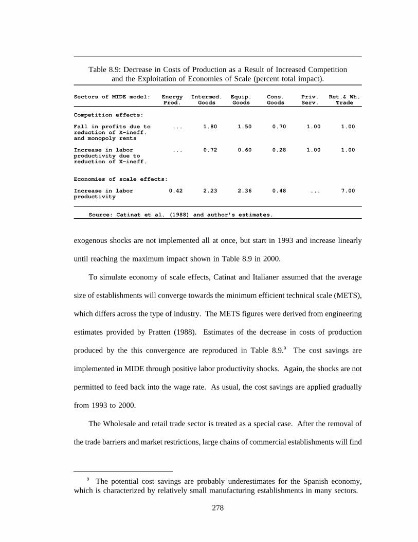
Table 8.9: Decrease in Costs of Production as a Result of Increased Competitionand the Exploitation of Economies of Scale (percent total impact).
Sectors of MIDE model: Energy Intermed. Equip. Cons. Priv. Ret.& Wh.Prod. Goods Goods Goods Serv. Trade
Competition effects:
Fall in profits due to ... 1.80 1.50 0.70 1.00 1.00reduction of X-ineff.and monopoly rents
Increase in labor ... 0.72 0.60 0.28 1.00 1.00productivity due toreduction of X-ineff.
Economies of scale effects:
Increase in labor 0.42 2.23 2.36 0.48 ... 7.00productivity
Source: Catinat et al. (1988) and author’s estimates.
exogenous shocks are not implemented all at once, but start in 1993 and increase linearly
until reaching the maximum impact shown in Table 8.9 in 2000.
To simulate economy of scale effects, Catinat and Italianer assumed that the average
size of establishments will converge towards the minimum efficient technical scale (METS),
which differs across the type of industry. The METS figures were derived from engineering
estimates provided by Pratten (1988). Estimates of the decrease in costs of production
produced by the this convergence are reproduced in Table 8.9.9 The cost savings are
implemented in MIDE through positive labor productivity shocks. Again, the shocks are not
permitted to feed back into the wage rate. As usual, the cost savings are applied gradually
from 1993 to 2000.
The Wholesale and retail trade sector is treated as a special case. After the removal of
the trade barriers and market restrictions, large chains of commercial establishments will find
9 The potential cost savings are probably underestimates for the Spanish economy,which is characterized by relatively small manufacturing establishments in many sectors.
278

Table 8.10: Supply Effects - Comparison to Spain With Borders Case.(1980 prices, except where otherwise indicated.)
1993 1994 1995 1996 1997 1998 1999 2000Percentage deviations
Gross domestic product 0.07 0.29 0.58 0.93 1.28 1.64 1.98 2.31Private national consumption 0.03 0.25 0.48 0.72 0.99 1.28 1.52 1.77Fixed capital investment 0.05 0.36 0.75 1.18 1.56 1.83 2.07 2.26Exports 0.12 0.36 0.67 1.01 1.43 1.83 2.25 2.60Imports -0.03 0.18 0.31 0.49 0.61 0.68 0.67 0.68
GDP deflator -0.44 -0.83 -1.28 -1.82 -2.40 -2.93 -3.51 -3.98Private consumption deflator -0.35 -0.67 -1.06 -1.48 -1.96 -2.42 -2.95 -3.32Fixed investment deflator -0.31 -0.56 -0.83 -1.18 -1.50 -1.91 -2.28 -2.55Export deflator -0.36 -0.64 -0.99 -1.37 -1.76 -2.15 -2.60 -2.95Import deflator 0.01 0.04 0.06 0.07 0.09 0.10 0.11 0.11
Real disp. income per capita -0.03 0.11 0.36 0.58 0.84 1.08 1.34 1.58Aggregate labor productivity 0.29 0.58 0.86 1.19 1.40 1.66 1.91 2.16Real wage rate 0.24 0.33 0.51 0.76 1.07 1.35 1.71 2.02Employment -0.22 -0.29 -0.28 -0.21 -0.11 -0.01 0.06 0.12
Absolute deviations
Current account deficit 0.05 0.12 0.17 0.23 0.28 0.32 0.33 0.37(% of GDP, current prices)Government deficit 0.05 0.02 -0.04 -0.12 -0.21 -0.30 -0.40 -0.50(% of GDP, current prices)Employment (thousands) -28.89 -38.18 -37.05 -28.13 -15.06 -1.73 8.05 16.75Unemployment rate (%) 0.19 0.25 0.24 0.18 0.09 0.01 -0.05 -0.10Long term interest rate (%) -0.27 -0.42 -0.44 -0.52 -0.63 -0.70 -0.83 -0.81
it easier to enter each domestic market. The average size of the establishments and the
efficiency in which they are operated will increase dramatically, especially in Spain. Indeed,
as I mentioned in Chapter 2, the phenomena is already noticeable. Commercial margins in
Spain have a long way to go toward convergence with those of partner nations with large
established chains. Therefore, the expected reduction in costs is projected to be much larger
than in the other sectors, reaching 7.0 percent by the year 2000.
Table 8.10 presents the results of introducing these shocks into the MIDE model. The
effect on domestic prices is major, the GDP deflator is down almost 3.0 percent by 1998.
The productivity shocks produce a predictable decrease in employment by 37 thousand jobs
by 1995. After that, increased growth in the economy creates enough jobs so that by 1999
the net effect is positive. Again, the bad news is in the foreign account. Real exports
expand at a much higher rate than imports, implying a marked improvement in the real trade
279

balance. However, the large reduction in prices received for exports creates the net effect
of increasing the nominal current account balance by .32 percent of GDP by 1998.
Fiscal Harmonization
The Value Added Tax is the major consumption tax for each of the European
Community nations. At the present time, however, the applicable tax rates vary significantly
from country to country. Large variations are also present for excise taxes on alcoholic
beverages and tobacco products. The disparity among tax rates has created fears that the
elimination of borders will entice consumers to make extensive purchases in other EC states.
In high-tax countries, the fiscal authorities would lose revenue and the producers would be
placed at a significant disadvantage. To address this problem, the Europe 1992 program
calls for approximate harmonization of VAT and excise tax rates. The present plan is for
the establishment of two bands of VAT rates, one from 4 to 9 percent for necessities and
the other from 14 to 20 percent for other goods. The deadline for fiscal harmonization has
been allowed to slip by a year or two.
Spanish VAT rates on several products are currently outside the bands, and
harmonization will have to occur eventually. There are three basic VAT rates in Spain. The
lowest rate of 6 percent covers food and other necessities. After a 1 percent increase,
effective January 1, 1992,10 the majority of other products are taxed at 13 percent. This
rate is one point below the 14 percent threshold of the proposed European upper band.
Another rate of 28 percent is applied to luxury goods, conspicuously including automobiles.
10 All of the model alternatives include the changes in the VAT rates which becameeffective in 1992. In the case of luxury goods, the rate was lowered from 33 percent to 28percent. When the final forecast is presented in the next section, it will be seen that the neteffect of these VAT rate changes is that inflation continues at a stubbornly high rate of 5.7percent. This is down only half a percentage point from 1991.
280

This rate will have to come down to at least 20 percent. Also, Spanish excise taxes on
alcoholic beverages and tobacco products are well below the EC norm, and it appears that
these will be raised eventually.
To simulate the expected harmonization, I changed the VAT rates, starting in 1995, to
conform with the current EC proposals. The rate on the middle band of products is
increased from 13 to 14 percent in 1995. The present 28 percent rate on luxuries is adjusted
downward to the 20 percent threshold, by 4 percentage points in 1995 and 4 points in 1996.
Additionally, to simulate increases in excise taxes on alcoholic beverages and tobacco
products, the indirect tax rates on these sectors were raised. For the beverage sector the
indirect tax rate was increased by a total of 10 percent (that is, 10 percent of the original tax
rate, not in percentage points), 5 percent in 1995 and 5 percent in 1996. The indirect tax
rate increase in the tobacco sector was 20 percent of the original rate, 10 percent in 1995
and 10 percent in 1996.
The results for fiscal harmonization appear in Table 8.11. The increased tax rates push
up prices and have a detrimental effect on growth. The most interesting long-run result is
that the government deficit, again as a percentage of GDP, increases slightly starting in
1997. This is because the employment loss, which totals almost 57 thousands jobs by 1998,
reduces both consumption, the base of the VAT tax, and income tax receipts. The results
call into question the use of VAT rate increases for the purposes of balancing the public
accounts.
281

Table 8.11: Fiscal Harmonization - Comparison to Spain With Borders Case.(1980 prices, except where otherwise indicated.)
1993 1994 1995 1996 1997 1998 1999 2000
Percentage deviations
Gross domestic product 0.00 0.00 -0.11 -0.31 -0.38 -0.40 -0.41 -0.37Private national consumption 0.00 0.00 -0.17 -0.43 -0.41 -0.43 -0.49 -0.43Fixed capital investment 0.00 0.00 -0.10 -0.42 -0.50 -0.50 -0.41 -0.26Exports 0.00 0.00 -0.07 -0.16 -0.23 -0.33 -0.34 -0.34Imports 0.00 0.00 -0.14 -0.43 -0.25 -0.31 -0.35 -0.24
GDP deflator 0.00 0.00 0.49 0.46 0.52 0.65 0.62 0.64Private consumption deflator 0.00 0.00 0.42 0.40 0.54 0.63 0.55 0.60Fixed investment deflator 0.00 0.00 0.43 0.42 0.53 0.48 0.49 0.52Export deflator 0.00 0.00 0.20 0.14 0.26 0.26 0.24 0.30Import deflator 0.00 0.00 -0.00 -0.01 0.01 0.01 0.01 0.02
Real disp. income per capita 0.00 0.00 -0.04 -0.30 -0.37 -0.39 -0.37 -0.36Aggregate labor productivity 0.00 0.00 0.00 0.00 0.00 0.00 0.00 0.00Real wage rate 0.00 0.00 -0.32 -0.19 -0.24 -0.34 -0.34 -0.38Employment 0.00 0.00 -0.10 -0.29 -0.36 -0.42 -0.44 -0.40VAT yield (current prices) 0.00 0.00 3.24 1.56 1.74 1.88 1.86 1.96
Absolute deviations
Average VAT rate (%) (a) 0.00 0.00 0.26 0.14 0.15 0.15 0.17 0.17
Current account deficit 0.00 0.00 -0.07 -0.11 -0.08 -0.06 -0.07 -0.05(% of GDP, current prices)Government deficit 0.00 0.00 -0.13 -0.01 0.01 0.02 0.03 0.02(% of GDP, current prices)Employment (thousands) 0.00 0.00 -12.57 -38.18 -48.64 -56.83 -60.21 -55.06Unemployment rate (%) 0.00 0.00 0.08 0.24 0.31 0.35 0.37 0.34Long term interest rate (%) 0.00 0.00 0.26 0.08 0.02 0.12 0.04 0.05
(a) - Nominal VAT taxes divided by nominal Private interior consumption.
Spain in the Single Market - The Total Impact
Table 8.12 illustrates the total effects of loading all of the above-described shocks into
the MIDE model. The macroeconomic impact is certainly significant. By 1998 the
difference in GDP is 4.0 percent, consumption is up 3.9 percent, and investment expands
by 4.8 percent. A favorable impact on the real trade balance is also evident: exports are
increased by 5.8 percent by 1998 while imports are higher by only 4.4 percent. The
difference in employment is 217 thousand jobs (1.6 percent) knocking 1.4 percentage points
from the unemployment rate.
Greater impacts are evident on the price side of the ledger. By 1998, the GDP deflator
is down by 7.6 percent and consumption prices by 6.7 percent. Lower prices contribute to
282

Table 8.12: Spain in the European Single Market:The Total Impact of Europe 1992 - Comparison to Spain With Borders Case. (1980
prices, except where otherwise indicated).
1993 1994 1995 1996 1997 1998 1999 2000Percentage deviations
Gross domestic product 0.15 0.68 1.28 1.93 2.86 3.97 5.21 6.65Private national consumption 0.22 0.92 1.37 1.69 2.73 3.90 4.93 6.15Fixed capital investment 0.20 1.04 1.89 2.61 3.68 4.78 6.03 7.34Exports 0.66 1.72 2.56 3.40 4.51 5.84 7.39 8.68Imports 0.61 1.83 2.24 2.49 3.48 4.39 4.99 5.35
GDP deflator -1.05 -1.95 -2.55 -4.27 -5.87 -7.65 -9.88 -11.95Private consumption deflator -1.08 -1.84 -2.41 -3.80 -5.15 -6.72 -8.68 -10.18Fixed investment deflator -1.18 -1.88 -2.30 -3.49 -4.69 -6.29 -7.86 -9.15Export deflator -1.89 -2.65 -3.34 -4.47 -5.70 -7.22 -8.82 -10.09Import deflator -1.46 -1.75 -1.51 -1.44 -2.13 -3.00 -2.98 -2.06
Real disp. income per capita 0.19 0.61 1.15 1.47 2.12 2.99 3.83 4.56Aggregate labor productivity 0.41 0.87 1.20 1.65 1.96 2.32 2.73 3.13Real wage rate 0.39 0.29 0.12 0.72 0.90 1.17 1.72 2.15Employment -0.28 -0.15 0.04 0.31 0.88 1.60 2.39 3.38
Absolute deviations
Current account deficit 0.09 0.23 0.38 0.56 0.72 0.87 1.13 1.54(% of GDP, current prices)Government deficit 0.02 -0.12 -0.42 -0.51 -0.79 -1.16 -1.52 -1.93(% of GDP, current prices)Employment (thousands) -35.58 -18.88 5.49 40.66 118.40 217.40 329.62 470.30Unemployment rate (%) 0.23 0.12 -0.04 -0.26 -0.75 -1.36 -2.04 -2.89Long term interest rate (%) -0.72 -1.05 -0.76 -1.39 -1.96 -2.27 -2.87 -2.97
a 2.2 point reduction in the interest rate. Stronger growth and lower interest rates have a
positive effect on the government balance, decreasing the nominal deficit by 1.52 percent
of the GDP. As in several of the individual scenarios, a deterioration of the terms of trade
occurs, with export prices declining by 7.2 percent but import prices decreasing by only 3.0
percent. This is a reasonable expectation. If one believes that present price rigidities in the
Spanish economy are stronger than those in its EC partners, then market integration will
produce greater price reductions on domestic prices than imported prices. Moreover, Spain
will still be importing significant quantities of goods, especially crude oil, from third
countries. EC integration will have little impact on the export prices from these countries.
This development causes a deterioration of the current account deficit of .87 percent of the
GDP by 1998.
283

Table 8.13: Europe 1992: Comparison Among MIDE and Other Studies.
Cons. Govt. External RealGDP Defl. Employ. Surp.(a) Bal.(b) Income(c)
Spain-MIDE (1998) 3.97 -6.72 1.60 1.16 -0.87 2.99
Catinat (6th yr.):EC Tot 4.52 -6.16 1.47 2.22 -0.35 2.94Germany 4.20 -6.16 1.68 1.52 0.15 3.27France 5.05 -4.89 1.57 2.64 -0.03 2.41Italy 3.79 -7.07 1.40 3.65 -1.89 3.50UK 2.91 -7.43 1.39 1.80 -0.21 2.80
Christou & Nyhus (1998):Germany 4.99 -8.19 0.23 ... ... 6.30France 4.84 -4.22 0.60 ... ... 4.20Italy 3.47 -5.52 -1.28 ... ... 3.94Belgium 5.66 ... 0.81 ... ... 4.06
Sources: Catinat et al. (1988, pp.617-623), Christou and Nyhus (1992).
Notes: Percentage deviations of total impact with respect to No-1992cases for GDP, consumption deflator, employment and real income.Government deficit and external balance are in absolutedeviations as percent of GDP.
(a) For MIDE, Govt. surplus is expressed in nominal terms, forCatinat et al., it is in real terms. Results not available forChristou and Nyhus.
(b) Nominal gross operating surplus over nominal GDP. Results notavailable for Christou and Nyhus.
(c) For Catinat, real household income; for others, real nationalincome per capita.
To place the macroeconomic results in perspective, Table 8.13 presents a comparison
of the MIDE generated results for the total impact of the scenarios with comparable figures
from Catinat et al. (1988) and Christou and Nyhus (1992). The countries included for each
study are the ones for which full results are available. The figures from CN and the present
study refer to 1998, and were computed by running the respective models with all of the
Europe 1992 shocks incorporated. The Catinat figures refer to the sixth year. Presuming
the EC-1992 program begins on time in 1993, this would also be 1998. Also for Catinat,
the total impact results represent the summation of the individual scenario results. The row
of Catinat corresponding to the total EC-12 effects is their extrapolation of the country
284

results to the entire community (p. 598). The results from this study seem to coincide with
the other two.
Tables 8.14 through 8.16 show the sectoral-level, percentage impacts for output, output
prices, employment, exports and imports for the total impact of the single market. Each
table ranks the sectors according to the magnitude of the effects in 1998. Figure 8.1 contrasts
graphs of domestic demand and output for twelve selected sectors. Virtually every sector
enjoys a positive impact of the single market program by 1998. The exceptions are
Agricultural and industrial machinery (Sector 10), which suffers significant import
penetration, and Tobacco products (19), which is hit with tax increases. Several sectors,
however, end up lower employment because of the productivity shocks. In general, the
industries experiencing the largest positive gains in production tend to be ones that have a
large component of consumer durables consumption. The greater levels of real disposable
incomes generated in the single market scenario touches of a consumer splurge in durable
goods such as electric appliances (affecting Sector 12), furniture (22) and automobiles (13).
The Electric and electronic materials industry (12) also benefits from significant
productivity and price shocks in both the Public procurement and Supply effects scenarios.
Therefore, its production price falls steeply, further stimulating demand for its products.
However, this performance should be set against a negative output growth in both 1990 and
1991 and a pessimistic projection in the Spain with Borders scenario. Even in the more
optimistic case of the Single Market alternative the output of the industry does not again
reach its 1989 peak level of production until 1995 (Figure 8.1). Moreover, it is clear from
the graph that the domestic industry continues to suffer from import penetration through the
mid-90’s. Another sector which experiences a reversal of fortune is the Textile and apparel
285

Table 8.14: Sectoral Real Outputs and the European Single Market -Comparison to Spain With Borders Case.
Percentage deviations of Single Market to Spain with Borders.Ranked according to figure for 1998.
Rank No. Sector 1994 1996 1998 2000
1. (12) Elect.& electronic prod. 0.99 4.62 11.00 19.452. (22) Wood & furniture 1.20 5.11 10.29 19.153. (20) Textiles & apparel 0.62 3.38 8.27 17.124. (23) Paper & publishing 0.60 3.71 7.28 13.695. (13) Automotive vehicles 2.74 3.83 7.21 9.69
6. ( 2) Coal & lignite 0.90 3.53 7.05 11.837. (25) Other mfg. products 1.73 3.08 6.95 10.658. (11) Off mach, comput, instr. 0.34 3.63 6.77 11.599. ( 6) Metal mining & proc. 1.03 3.47 6.72 11.74
10. (14) Other transport equip. 0.73 3.63 6.49 10.31
11. (27) Repairs & reconstruct. 1.73 2.97 6.42 9.5012. (38) Priv. health services 1.30 2.79 6.09 9.9113. ( 1) Agriculture, forest. & fish 1.27 3.02 5.81 9.3414. ( 3) Coke products 0.75 2.89 5.79 10.1415. (21) Shoes & leather prod. 0.47 2.76 5.76 9.88
16. (31) Maritime & air transp. 1.39 3.00 5.61 8.7717. (43) Domest. & oth. services 1.01 2.37 5.60 9.4718. (37) Priv. educ. & research 1.11 2.45 5.46 8.9719. (35) Business services 1.06 2.63 5.40 8.9220. (34) Banking & insurance 0.85 2.74 5.24 8.69
21. (33) Communications 1.17 2.38 5.08 8.0422. (28) Wholesale & ret. trade 1.19 2.23 4.95 7.8223. (39) Cult. & oth. services 0.84 2.18 4.75 8.0024. (30) Interior transport 1.00 2.25 4.71 7.5625. (17) Other food products 0.60 2.45 4.63 7.92
Average 0.72 2.16 4.59 7.92
26. ( 9) Metal products 0.76 2.04 4.25 7.1027. ( 5) Electric & oth. util. 0.70 1.97 4.14 7.2128. (18) Beverages 0.31 2.03 4.12 7.3329. (24) Rubber & plastic prod. 0.51 1.81 4.02 7.3230. (29) Rest., cafes & hotels 1.13 1.73 3.94 6.02
31. (26) Construction 0.57 1.91 3.47 5.6232. ( 7) Nonmetal mining & prod. 0.31 1.75 3.46 6.1633. (32) Oth. transport serv. 0.80 1.86 3.41 5.5234. ( 8) Chemicals 0.30 1.37 2.88 4.9535. (15) Meat & oth. animal prod. 0.06 1.39 2.80 5.21
36. ( 4) Petroleum products 0.11 1.29 2.56 4.0637. (16) Dairy Products -0.07 0.64 1.50 2.8138. (36) Commerc. & resid. rents -0.78 0.53 0.63 2.4339. (41) Pub. education 0.02 0.05 0.11 0.1940. (40) Pub. administration 0.01 0.03 0.07 0.12
41. (42) Pub. health services 0.00 0.01 0.02 0.0342. (10) Agric. & indust. mach. -0.38 -0.44 -0.07 0.4943. (19) Tobacco products 0.04 -4.14 -3.44 -0.02
286
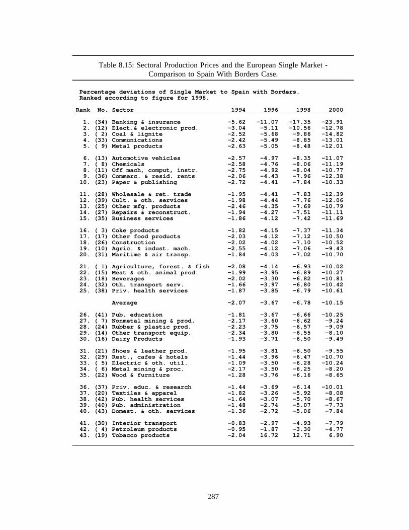
Table 8.15: Sectoral Production Prices and the European Single Market -Comparison to Spain With Borders Case.
Percentage deviations of Single Market to Spain with Borders.Ranked according to figure for 1998.
Rank No. Sector 1994 1996 1998 2000
1. (34) Banking & insurance -5.62 -11.07 -17.35 -23.912. (12) Elect.& electronic prod. -3.04 -5.11 -10.56 -12.783. ( 2) Coal & lignite -2.52 -5.68 -9.86 -14.824. (33) Communications -2.42 -5.49 -8.85 -13.015. ( 9) Metal products -2.63 -5.05 -8.48 -12.01
6. (13) Automotive vehicles -2.57 -4.97 -8.35 -11.077. ( 8) Chemicals -2.58 -4.76 -8.06 -11.198. (11) Off mach, comput, instr. -2.75 -4.92 -8.04 -10.779. (36) Commerc. & resid. rents -2.06 -4.43 -7.96 -12.38
10. (23) Paper & publishing -2.72 -4.41 -7.84 -10.33
11. (28) Wholesale & ret. trade -1.95 -4.41 -7.83 -12.3912. (39) Cult. & oth. services -1.98 -4.44 -7.76 -12.0613. (25) Other mfg. products -2.46 -4.35 -7.69 -10.7914. (27) Repairs & reconstruct. -1.94 -4.27 -7.51 -11.1115. (35) Business services -1.86 -4.12 -7.42 -11.69
16. ( 3) Coke products -1.82 -4.15 -7.37 -11.3417. (17) Other food products -2.03 -4.12 -7.12 -10.5018. (26) Construction -2.02 -4.02 -7.10 -10.5219. (10) Agric. & indust. mach. -2.55 -4.12 -7.06 -9.4320. (31) Maritime & air transp. -1.84 -4.03 -7.02 -10.70
21. ( 1) Agriculture, forest. & fish -2.08 -4.14 -6.93 -10.0222. (15) Meat & oth. animal prod. -1.99 -3.95 -6.89 -10.2723. (18) Beverages -2.02 -3.30 -6.82 -10.8124. (32) Oth. transport serv. -1.66 -3.97 -6.80 -10.4225. (38) Priv. health services -1.87 -3.85 -6.79 -10.61
Average -2.07 -3.67 -6.78 -10.15
26. (41) Pub. education -1.81 -3.67 -6.66 -10.2527. ( 7) Nonmetal mining & prod. -2.17 -3.60 -6.62 -9.2428. (24) Rubber & plastic prod. -2.23 -3.75 -6.57 -9.0929. (14) Other transport equip. -2.34 -3.80 -6.55 -8.1030. (16) Dairy Products -1.93 -3.71 -6.50 -9.49
31. (21) Shoes & leather prod. -1.95 -3.81 -6.50 -9.5532. (29) Rest., cafes & hotels -1.44 -3.96 -6.47 -10.7033. ( 5) Electric & oth. util. -1.09 -3.50 -6.28 -10.2434. ( 6) Metal mining & proc. -2.17 -3.50 -6.25 -8.2035. (22) Wood & furniture -1.28 -3.76 -6.16 -8.65
36. (37) Priv. educ. & research -1.44 -3.69 -6.14 -10.0137. (20) Textiles & apparel -1.82 -3.26 -5.92 -8.0838. (42) Pub. health services -1.64 -3.07 -5.70 -8.6739. (40) Pub. administration -1.48 -2.74 -5.07 -7.7340. (43) Domest. & oth. services -1.36 -2.72 -5.06 -7.84
41. (30) Interior transport -0.83 -2.97 -4.93 -7.7942. ( 4) Petroleum products -0.95 -1.87 -3.30 -4.7743. (19) Tobacco products -2.04 16.72 12.71 6.90
287
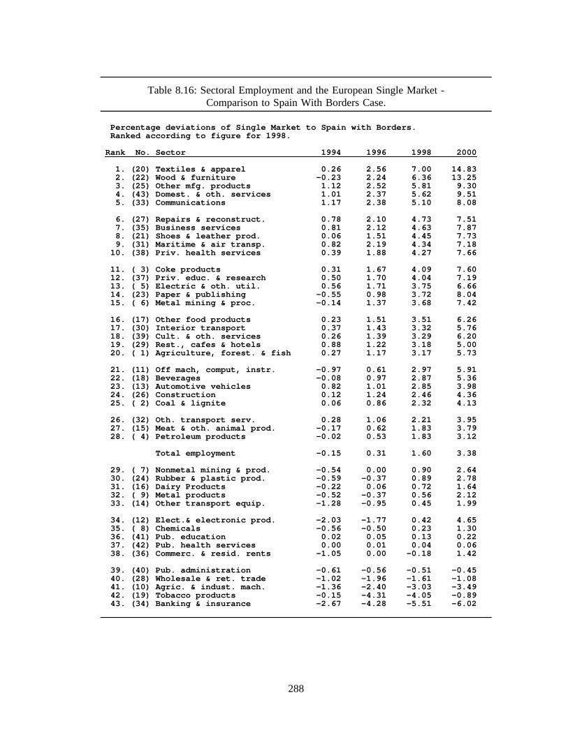
Table 8.16: Sectoral Employment and the European Single Market -Comparison to Spain With Borders Case.
Percentage deviations of Single Market to Spain with Borders.Ranked according to figure for 1998.
Rank No. Sector 1994 1996 1998 2000
1. (20) Textiles & apparel 0.26 2.56 7.00 14.832. (22) Wood & furniture -0.23 2.24 6.36 13.253. (25) Other mfg. products 1.12 2.52 5.81 9.304. (43) Domest. & oth. services 1.01 2.37 5.62 9.515. (33) Communications 1.17 2.38 5.10 8.08
6. (27) Repairs & reconstruct. 0.78 2.10 4.73 7.517. (35) Business services 0.81 2.12 4.63 7.878. (21) Shoes & leather prod. 0.06 1.51 4.45 7.739. (31) Maritime & air transp. 0.82 2.19 4.34 7.18
10. (38) Priv. health services 0.39 1.88 4.27 7.66
11. ( 3) Coke products 0.31 1.67 4.09 7.6012. (37) Priv. educ. & research 0.50 1.70 4.04 7.1913. ( 5) Electric & oth. util. 0.56 1.71 3.75 6.6614. (23) Paper & publishing -0.55 0.98 3.72 8.0415. ( 6) Metal mining & proc. -0.14 1.37 3.68 7.42
16. (17) Other food products 0.23 1.51 3.51 6.2617. (30) Interior transport 0.37 1.43 3.32 5.7618. (39) Cult. & oth. services 0.26 1.39 3.29 6.2019. (29) Rest., cafes & hotels 0.88 1.22 3.18 5.0020. ( 1) Agriculture, forest. & fish 0.27 1.17 3.17 5.73
21. (11) Off mach, comput, instr. -0.97 0.61 2.97 5.9122. (18) Beverages -0.08 0.97 2.87 5.3623. (13) Automotive vehicles 0.82 1.01 2.85 3.9824. (26) Construction 0.12 1.24 2.46 4.3625. ( 2) Coal & lignite 0.06 0.86 2.32 4.13
26. (32) Oth. transport serv. 0.28 1.06 2.21 3.9527. (15) Meat & oth. animal prod. -0.17 0.62 1.83 3.7928. ( 4) Petroleum products -0.02 0.53 1.83 3.12
Total employment -0.15 0.31 1.60 3.38
29. ( 7) Nonmetal mining & prod. -0.54 0.00 0.90 2.6430. (24) Rubber & plastic prod. -0.59 -0.37 0.89 2.7831. (16) Dairy Products -0.22 0.06 0.72 1.6432. ( 9) Metal products -0.52 -0.37 0.56 2.1233. (14) Other transport equip. -1.28 -0.95 0.45 1.99
34. (12) Elect.& electronic prod. -2.03 -1.77 0.42 4.6535. ( 8) Chemicals -0.56 -0.50 0.23 1.3036. (41) Pub. education 0.02 0.05 0.13 0.2237. (42) Pub. health services 0.00 0.01 0.04 0.0638. (36) Commerc. & resid. rents -1.05 0.00 -0.18 1.42
39. (40) Pub. administration -0.61 -0.56 -0.51 -0.4540. (28) Wholesale & ret. trade -1.02 -1.96 -1.61 -1.0841. (10) Agric. & indust. mach. -1.36 -2.40 -3.03 -3.4942. (19) Tobacco products -0.15 -4.31 -4.05 -0.8943. (34) Banking & insurance -2.67 -4.28 -5.51 -6.02
288

Table 8.17: Real Sectoral Exports and the European Single Market -Comparison to Spain With Borders Case.
Percentage deviations of Single Market to Spain with Borders.Ranked according to figure for 1998.
Rank No. Sector 1994 1996 1998 2000
1. ( 9) Metal products 4.37 10.46 18.78 29.642. (20) Textiles & apparel 2.66 6.20 10.20 15.423. ( 1) Agriculture, forest. & fish 3.58 5.49 8.32 11.714. ( 6) Metal mining & proc. 2.59 5.04 7.93 11.795. (17) Other food products 1.90 4.10 7.19 11.18
6. (18) Beverages 1.76 3.43 7.17 13.047. (22) Wood & furniture 1.13 3.99 6.99 11.368. (23) Paper & publishing 2.02 3.61 6.34 9.019. (13) Automotive vehicles 2.34 4.33 6.34 8.88
10. (10) Agric. & indust. mach. 2.02 3.89 6.25 9.18
Total exports 1.72 3.40 5.84 8.68
11. (28) Wholesale & ret. trade 1.54 2.97 4.84 7.2412. (14) Other transport equip. 0.98 2.49 4.41 6.2613. (32) Oth. transport serv. 1.32 2.56 4.21 6.3614. (12) Elect.& electronic prod. 1.10 2.20 3.69 5.4615. (30) Interior transport 1.11 2.17 3.61 5.51
16. (31) Maritime & air transp. 1.05 2.06 3.43 5.2517. ( 8) Chemicals 0.92 1.79 2.87 4.1618. (25) Other mfg. products 0.38 0.86 1.63 2.5919. (21) Shoes & leather prod. 0.38 0.76 1.24 1.8120. (11) Off mach, comput, instr. 0.20 0.47 0.74 1.02
21. ( 3) Coke products 0.00 0.00 0.14 0.2722. ( 2) Coal & lignite 0.00 0.00 0.06 0.1223. (41) Pub. education 0.00 0.00 0.00 0.0024. (24) Rubber & plastic prod. 0.00 -0.04 -0.09 -0.1825. ( 5) Electric & oth. util. -0.04 -0.10 -0.12 -0.17
26. (15) Meat & oth. animal prod. -0.04 -0.12 -0.22 -0.3627. (16) Dairy Products -0.05 -0.14 -0.26 -0.4228. (35) Business services -0.10 -0.23 -0.41 -0.6629. (34) Banking & insurance -0.10 -0.23 -0.41 -0.6630. (33) Communications -0.10 -0.23 -0.41 -0.66
31. (39) Cult. & oth. services -0.11 -0.23 -0.42 -0.6532. ( 4) Petroleum products -0.21 -0.59 -0.67 -0.9333. ( 7) Nonmetal mining & prod. -0.67 -0.95 -1.41 -1.8334. (19) Tobacco products 0.92 -6.93 -9.79 -6.70
289

Table 8.18: Real Sectoral Imports and the European Single Market -Comparison to Spain With Borders Case.
Percentage deviations of Single Market to Spain with Borders.Ranked according to figure for 1998.
Rank No. Sector 1994 1996 1998 2000
1. (14) Other transport equip. 7.45 16.14 24.82 35.972. (10) Agric. & indust. mach. 3.05 6.41 11.20 16.133. ( 3) Coke products 2.08 6.02 11.19 18.234. ( 9) Metal products 3.13 6.64 11.17 16.295. (13) Automotive vehicles 4.12 6.21 10.88 14.12
6. (19) Tobacco products -0.48 3.59 8.12 9.127. ( 8) Chemicals 1.88 3.39 6.75 10.418. (20) Textiles & apparel 4.14 3.30 6.17 4.809. (18) Beverages 4.39 4.36 6.05 4.17
10. (32) Oth. transport serv. 1.66 3.03 6.04 9.00
11. ( 6) Metal mining & proc. 2.14 3.45 5.86 7.6712. (30) Interior transport 1.22 2.82 5.73 8.9613. (39) Cult. & oth. services 1.04 2.59 5.55 9.2614. (33) Communications 1.13 2.20 4.81 7.6615. (12) Elect.& electronic prod. 3.06 2.87 4.44 3.6916. ( 5) Electric & oth. util. 0.92 2.14 4.41 7.60
Total imports 1.83 2.49 4.78 7.34
17. (17) Other food products 2.36 2.30 4.18 4.0918. ( 4) Petroleum products 0.67 1.68 3.31 5.1319. (16) Dairy Products 1.04 1.24 3.11 3.2820. (24) Rubber & plastic prod. 1.51 1.73 2.95 2.5821. (28) Wholesale & ret. trade 1.38 0.71 1.57 0.38
22. ( 7) Nonmetal mining & prod. 0.86 0.90 1.17 0.1923. (25) Other mfg. products 0.46 -0.08 0.39 -0.0924. ( 2) Coal & lignite -0.04 -0.09 0.01 0.2625. (41) Pub. education 0.00 0.00 0.00 0.0026. (23) Paper & publishing 1.12 -0.28 0.00 -2.20
27. (15) Meat & oth. animal prod. 1.25 0.34 -0.09 -2.8028. ( 1) Agriculture, forest. & fish 0.35 -0.24 -0.71 -1.2929. (11) Off mach, comput, instr. 0.47 -0.47 -0.88 -2.0530. (22) Wood & furniture 2.56 -1.27 -2.17 -7.5231. (35) Business services -0.53 -1.52 -2.99 -5.26
32. (21) Shoes & leather prod. -0.06 -1.71 -3.48 -7.6533. (31) Maritime & air transp. -2.04 -4.78 -7.87 -12.0334. (34) Banking & insurance -3.25 -6.08 -9.22 -12.18
industry (20), because of both stronger consumption and export growth. Whether the
Europe-1992 program turns out to be such a large boon to the Spanish economy is yet to
be seen. Assuming this story is realistic, let us now turn to examining the economic
projection which it produces.
290
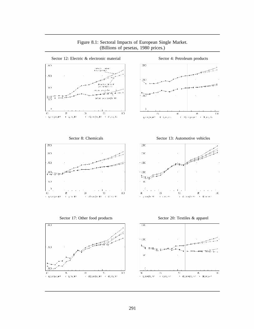
Figure 8.1: Sectoral Impacts of European Single Market.(Billions of pesetas, 1980 prices.)
Sector 12: Electric & electronic material Sector 4: Petroleum products
Sector 8: Chemicals Sector 13: Automotive vehicles
Sector 17: Other food products Sector 20: Textiles & apparel
291

Figure 8.1: Sectoral Impacts of European Single Market (continued).(Billions of pesetas, 1980 prices.)
Sector 22: Wood & furniture Sector 23: Paper & publishing
Sector 26: Construction Sector 28: Wholesale & retail trade
Sector 30: Interior transport Sector 34: Banks & insurance
292

8.3 A MIDE Forecast to the Year 2000
Table 8.19 displays the macroeconomic results from the total impact scenario. The
alternative is entitled Spain in the Single Market. The figures are shown in annual growth
rates. The table begins in the year 1990 to give the reader the opportunity to compare the
recent history with the forecast. This projection was made in April of 1992 and incorporates
all information available at that time. The macroeconomic results include the 1991
provisional estimates for GDP and its components made by the Instituto Nacional
Estadística. Also, consumer price, industrial production, industrial price and various other
indices available for 1991 are used in various ways to guide the projections for that year.
From 1992 through 1996, growth is very stable. The growth rate of GDP, which varies
between 2.5 and 3.0 percent in this period, is low compared to recent growth. (Although, it
is up from 1991, a recession year in other parts of the world.) The 1992-96 period is also
characterized by gradual a reduction in price inflation. The unemployment rate (second page
of Table 8.19) continues to decline through the period, albeit at an excruciatingly slow pace.
The slower growth, steady decreases in inflation and low rate of job formation are all
consequences, at least partly, of integration of the European market. Because of the removal
of tariff and non-tariff barriers, import price increases will be moderate and imports will
continue to displace domestic production, constraining overall growth. Stiffer competition
from abroad will force domestic firms to hold the line on price increases and enhance
productivity, moderating both price and employment growth. Finally, while export growth
promises to be healthy, it will not compensate for reduced capital formation, as investors take
a breather from the recent vigorous activity. The nominal current account deficit as a
percentage of GDP increases modestly.
293

Table 8.19: Spain in the Single Market, MIDE Forecast to 2000.
Gross Domestic Product and ComponentsAnnual percentage rate of growth, constant 1980 prices.
1990 1991 1992 1993 1994 1995 1996 1997 1998 1999 2000
Gross Domestic Product 3.62 2.37 2.76 2.86 2.96 2.84 2.60 3.49 3.70 3.69 3.85
Private National Consumption 3.76 3.13 3.66 4.13 3.98 3.41 3.51 3.94 3.94 3.50 3.63
Government Consumption * 4.24 4.53 3.98 1.98 1.98 1.98 1.98 1.98 1.98 1.98 1.98
Gross Fixed Investment 6.91 1.71 3.61 3.16 4.72 4.57 4.31 4.55 4.75 4.55 4.50Equipment 1.40 -2.40 5.03 3.21 4.86 4.32 4.05 4.71 4.65 4.21 4.53Residential Construction 7.01 -7.08 -0.30 3.32 4.23 3.05 4.38 4.80 4.71 4.14 3.60Non-residential Construction 12.72 9.64 3.90 3.06 4.79 5.34 4.50 4.31 4.84 4.99 4.81
Inventory Change (a) 0.16 0.06 -0.60 -0.35 -0.16 -0.24 -0.18 0.08 0.07 -0.00 0.08
Exports 3.23 8.53 7.08 7.00 5.03 5.27 4.90 4.90 5.81 6.03 6.51Merchandise Exports (fob) 5.44 8.99 7.11 7.37 6.10 6.00 5.41 5.19 6.08 6.03 6.08Service Exports 8.31 10.16 5.66 8.03 5.20 4.14 4.43 4.34 5.13 5.10 4.71Interior Cons. by Non-resid. -8.86 5.00 8.47 4.43 0.29 3.23 3.09 4.18 5.36 7.12 10.59
(Imports) 7.76 9.26 7.08 7.09 6.95 5.93 6.47 5.69 5.86 4.93 5.28(Merchandise Imports (cif)) 7.43 9.51 7.06 6.85 6.78 5.69 6.32 5.48 5.65 4.83 5.30(Service Imports) 9.85 9.16 6.84 11.44 9.95 9.38 9.28 8.90 8.87 6.27 5.47(Exterior Cons. of Residents) 13.17 3.10 8.02 6.12 6.10 5.87 5.10 5.00 5.21 4.96 4.28
GDP Deflator 7.30 6.89 6.37 5.73 4.84 4.36 3.40 2.92 3.28 2.64 3.23Private Consumption Deflator 6.44 6.21 5.73 4.28 3.75 3.44 2.64 2.38 2.70 2.14 2.87Fixed Investment Deflator 6.08 5.14 4.58 3.93 3.98 3.83 2.84 2.65 3.04 2.91 3.29Export Deflator 1.67 2.04 3.53 1.91 1.66 1.81 1.34 0.98 1.76 1.66 2.47Import Deflator -1.16 0.68 0.66 2.24 2.54 3.03 2.09 2.32 3.04 4.08 4.01
Real Trade Balance -7.99 -8.68 -9.04 -9.43 -10.24 -10.70 -11.48 -11.92 -12.18 -12.05 -11.90(const. prices, % of GDP)
Current Account Surplus -3.46 -3.08 -2.39 -2.40 -2.85 -3.18 -3.62 -4.05 -4.36 -4.70 -4.89(current prices, % of GDP)
Government Budget Surplus -3.87 -4.07 -3.65 -3.09 -2.59 -2.05 -1.80 -1.25 -0.55 0.06 0.78(current prices, % of GDP)
* - exogenous(a) - percentage change as a proportion of GDP

Table 8.19: Spain in the Single Market, MIDE Forecast to 2000 (continued).
Other macroeconomic variablesAnnual percentage rate of growth unless otherwise noted.
1990 1991 1992 1993 1994 1995 1996 1997 1998 1999 2000
Income and savings:Net National Disposable Income 10.93 9.31 9.64 8.94 8.08 7.33 6.12 6.53 7.19 6.40 7.25(current prices)
Household Net Disposable Income 12.65 8.93 8.55 8.06 7.46 6.82 6.00 6.13 6.71 6.11 6.85(current prices)
Household Savings Rate (%) 6.60 6.10 5.20 4.70 4.30 4.20 4.00 3.70 3.70 4.10 4.30Net National Disp. Income per cap 4.03 2.74 3.54 4.32 4.03 3.64 3.28 3.96 4.30 4.12 4.21(thous. of pts., constant prices)
Labor Market:Labor force 1.36 0.35 0.60 1.00 1.00 0.90 0.90 0.90 0.85 0.80 0.80Employment 2.61 0.24 0.68 1.12 1.28 1.29 1.24 1.65 1.99 2.01 2.16Unemployment rate (%) 16.25 16.34 16.28 16.18 15.95 15.63 15.34 14.71 13.75 12.71 11.53Nominal wages per worker 9.44 9.59 8.58 6.97 6.11 5.87 5.41 5.28 5.69 5.83 6.07Aggregate labor productivity 0.94 2.11 2.07 1.73 1.70 1.50 1.36 1.79 1.70 1.62 1.65Real wages per worker 1.99 2.52 2.09 1.17 1.20 1.45 1.94 2.31 2.33 3.11 2.75
Monetary Sector:ALP Broad Money Supply * 11.85 13.00 11.00 10.00 8.50 8.00 7.50 7.25 7.00 6.75 6.50M2 Narrow Money Supply * 17.77 12.00 11.00 10.00 8.50 8.00 7.50 7.25 7.00 6.75 6.50Long run interest rate (%) * 14.90 12.80 10.67 9.51 9.12 8.59 7.84 7.38 7.66 7.71 8.18
Exterior Sector:Avg. Foreign Dem. for Merch. 5.29 1.39 3.63 5.77 3.90 3.98 3.46 2.98 3.97 3.38 3.37Avg. Relat. Price of Merch. Exp. 3.86 0.27 -1.72 -1.56 -0.75 -0.85 -1.14 -1.34 -1.56 -2.08 -2.32Pesetas/German Mark * -1.43 -0.83 0.70 1.59 0.78 0.78 0.00 0.00 0.00 0.00 0.00Pesetas/Pounds Sterling * -6.64 3.79 -0.39 0.09 -0.69 -0.66 -1.40 0.00 -0.00 0.00 -0.00Pesetas/US Dollar * -13.91 2.33 -2.75 0.33 -0.49 -0.50 0.00 0.00 1.94 1.27 1.25
* - exogenous
Notes: Values for 1990 are advanced estimates of Instituto Nacional Estadística or actual. For 1991, majorcomponents of GDP, price deflators and wages are first estimations of INE; employment, money supply,interest and exchange rates are actual; all other variables are estimated or projected by the model.

Such an economic performance for the Spanish economy should qualify it for
membership in the European Economic and Monetary Union (EMU). The 1996 figures for
consumer inflation (2.64 percent), interest rates, (7.84 percent) and the government deficit
as a proportion of GDP (1.80 percent) would have easily qualified at the beginning of 1992.
However, this favorable results must be judged against several factors which underlie the
forecast.
First of all, the exogenous growth of government consumption is held to 2 percent per
year as proposed in the Convergence Plan. The government has missed its targets before,
often by a large margin. The regional governments have been especially profligate lately,
and neither the central government, nor the voters, have much control over this spending
(see Chapter 2). If spending were to grow by 3 percent of more, there would likely be
problems with the deficit target.
Second, the wage growth illustrated by this forecast is moderate, reflecting trend
established in the 1980’s. (Recall from Chapter 7 that the aggregate wage equation is
estimated from 1980-1990.) Real wages move generally in line with productivity and,
therefore, inflation is suppressed. However, ominous signs of labor unrest in early 1992
may mark a break with this behavior. If wages were to rise significantly faster than
projected here, inflation would reignite, extinguishing the prospects for nominal convergence.
A third outstanding question would be the course of currency movements. The
deterioration in the current account is shown as moderate here. If it were to be much worse,
downward pressure on the peseta could require a depreciation that would, technically,
eliminate EMU membership possibilities. One circumstance that could create such an
outcome would be sluggish overall growth in Europe that prevents Spanish exports from
expanding as indicated in the Table 3.19. Indeed, this forecast is based on a rosy scenario
296
of European harmony that stimulates European growth. However, if this assumption were
not realized, I expect that Spain would be one among a number of EC nations with
convergence problems.
The forecast displays a second tendency beginning in 1997. Growth increases sharply
to 3.5 to 4.0 percent from 1997 through 2000. One of the developments driving this
scenario is a sharp decrease in unemployment resulting from a slower growth rate of the
labor force. Also by this time, much of the job-destroying restructuring stimulated by the
Europe-1992 program will have been completed. The decreases in the unemployment rate
stimulate consumption. Despite the higher rates of growth, price inflation remains moderate.
The current account, however, begins to deteriorate sharply.
This final point raises and interesting question related to monetary union: If Spain does
join the monetary union, which involves a single currency for all of the EC, will the current
account be anything to worry about? At the national level the financing problem would
disappear. Indebtedness would then become an issue settled in a unified capital market by
individual parties. In the long-run, the increase in Spanish deficits may portend a problem
for the individual parties who have incurred the debts, be they consumers, corporations, or
government. If liquidity problems of this type were to occur, the optimistic growth forecast
presented here would probably not be realized.
The advantage of the MIDE model is its level of disaggregation. Therefore, the final
aspect of the forecast which deserves attention is its results for the various sectors and
industries of the economy. From these projections, we can gain an appreciation of how the
structure of the economy will change. Figure 8.2 shows the percentage shares of value
added and employment for the six major sectors of the economy for the years 1986, 1990,
1994 and 1998. The MIDE model does not project anything novel here, just a continuation
297

of established trends. The Spanish economy is expected to display the familiar pattern of
a maturing economy, an increasing share of production and employment in services at the
expense of agriculture and manufacturing. The construction industry appears to do well in
the forecast. It is spurred on by a high level of government investment in infrastructure and
strong residential construction growth.
Figure 8.3 displays the imports shares of domestic demand and export shares of
domestic production for 18 selected manufacturing industries. Again, we see a continuation
of many recent trends. Most sectors demonstrate increases in both ratios. The story told
by these graphs is of a nation steadily opening to world trade. Other results presented in
this chapter illustrate that the opening will be overwhelmingly beneficial for the economic
welfare of the people of Spain.
As a final parting shot, I leave the reader with Tables 8.20 through 8.30. These present
detailed sectoral level results of the forecast for various variables. These tables are a portion
of the standard output of the MIDE model, which can be perused, or not, at the readers
leisure.
298

Figure 8.2: Value Added and Employment Shares by Major Sectors,1986, 1990, 1994, 1998. (Percent)
Sector 1: Agriculture, forest & fish Sectors 2-5: Energy products
Sectors 6-25: Manufacturing Sector 26: Construction
Sectors 27-39: Market Services Sector 40-43: Government & Non-mkt serv.
Note: For 1994 and 98, bar with diagonal lines represents Spain with Borders alternative.Solid bar is Spain in Single Market forecast.
299
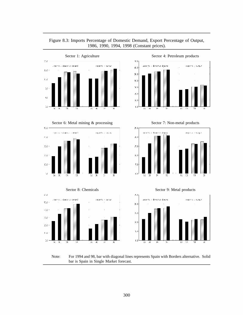
Figure 8.3: Imports Percentage of Domestic Demand, Export Percentage of Output,1986, 1990, 1994, 1998 (Constant prices).
Sector 1: Agriculture Sector 4: Petroleum products
Sector 6: Metal mining & processing Sector 7: Non-metal products
Sector 8: Chemicals Sector 9: Metal products
Note: For 1994 and 98, bar with diagonal lines represents Spain with Borders alternative. Solidbar is Spain in Single Market forecast.
300

Figure 8.3: Imports Percentage of Domestic Demand, Export Percentage of Output,1986, 1990, 1994, 1998 (Constant prices) (continued).
Sector 10: Agricultural & industrial machinery Sector 11: Off. mach., computers & instruments
Sector 12: Electric & electronic material Sector 13: Automotive vehicles
Sector 14: Other transport equipment Sector 17: Other food products
Note: For 1994 and 98, bar with diagonal lines represents Spain with Borders case. Solid baris Single Market forecast.
301
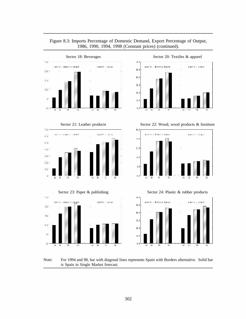
Figure 8.3: Imports Percentage of Domestic Demand, Export Percentage of Output,1986, 1990, 1994, 1998 (Constant prices) (continued).
Sector 18: Beverages Sector 20: Textiles & apparel
Sector 21: Leather products Sector 22: Wood, wood products & furniture
Sector 23: Paper & publishing Sector 24: Plastic & rubber products
Note: For 1994 and 98, bar with diagonal lines represents Spain with Borders alternative. Solid baris Spain in Single Market forecast.
302

Table 8.20: MIDE Model Projections - Constant Price Output by Production Sector.(Average annual percentage growth rates.)
88-90 90-92 92-94 94-96 96-98 98-100
AGRICULTURE, FOREST. & FISH -1.89 0.30 1.54 1.53 3.89 3.87
ENERGY PRODUCTS 5.73 1.75 1.32 2.15 3.36 3.832. Coal and lignite 5.58 -9.07 0.08 1.57 5.93 6.473. Coke products 3.93 -3.45 1.20 1.18 2.84 4.094. Petroleum products 7.10 2.61 0.88 1.60 2.43 2.935. Electric & oth. util. 3.84 2.35 2.14 3.10 4.44 4.78
MANUFACTURING 2.74 0.53 3.03 2.72 4.45 4.726. Metal mining & proc. 1.04 0.96 5.10 5.13 6.00 7.507. Nonmetal mining & prod. 4.21 -0.81 2.04 2.94 3.37 3.808. Chemicals 2.19 1.90 3.32 1.99 3.83 4.109. Metal products 5.60 -0.03 3.08 2.78 3.61 3.92
10. Agric. & indust. mach. 3.34 -5.04 0.86 1.57 2.01 2.2211. Off mach, comput, instr. 18.69 -1.21 5.06 7.24 8.26 8.6312. Elect.& electronic prod. -0.40 -1.86 2.84 3.88 4.76 5.4413. Automotive vehicles 2.76 2.43 6.65 4.81 6.14 5.5314. Other transport equip. 14.96 -0.22 1.42 0.93 1.92 2.3115. Meat & oth. animal prod. 1.76 0.88 1.27 0.94 3.35 2.9316. Dairy Products 5.20 -1.55 1.48 1.00 2.81 2.3817. Other food products 0.87 2.20 1.15 0.96 3.68 3.4718. Beverages 3.18 3.48 0.32 2.71 3.46 3.5319. Tobacco products -6.94 -0.65 3.04 -8.24 1.61 6.6120. Textiles & apparel 1.31 -3.95 0.19 0.66 1.92 3.2421. Shoes & leather prod. -1.69 0.54 4.51 -6.34 11.36 5.6122. Wood & furniture -0.92 -1.63 1.83 4.04 5.25 5.3623. Paper & publishing 3.06 2.31 3.50 3.72 5.23 6.2824. Rubber & plastic prod. -0.63 2.09 3.72 2.97 4.12 4.1325. Other mfg. products 9.44 6.36 6.49 5.25 5.84 5.38
CONSTRUCTION 14.84 3.48 3.39 4.05 4.10 4.25
MARKET SERVICES 5.18 3.51 4.32 3.79 4.49 4.6127. Repairs & reconstruct. 4.23 3.70 4.89 4.22 4.98 4.6728. Wholesale & ret. trade 4.19 3.53 3.80 3.24 4.12 4.1529. Rest., cafes & hotels 3.47 3.27 3.64 3.45 4.24 4.2130. Interior transport 5.91 3.39 4.32 3.90 4.88 4.8531. Maritime & air transp. 4.61 3.93 4.82 3.75 4.21 5.0432. Oth. transport serv. 3.23 3.04 2.45 1.84 2.31 3.0133. Communications 9.44 3.57 6.13 4.88 5.72 5.4934. Banking & insurance 11.65 4.75 5.82 5.13 6.00 6.0735. Business services 3.95 3.24 4.32 3.53 4.57 4.8536. Commerc. & resid. rents 2.92 2.53 3.69 3.51 3.17 3.6237. Priv. educ. & research 3.24 3.74 3.99 3.24 3.92 3.8138. Priv. health services 6.51 3.36 4.56 3.88 4.65 4.4539. Cult. & oth. services 4.18 3.95 5.36 4.42 5.03 4.88
NON-MARKET SERVICES 5.74 4.45 2.06 2.03 2.08 2.0840. Pub. administration 5.90 4.46 2.06 2.05 2.06 2.0541. Pub. education 6.65 4.73 1.97 1.96 1.98 1.9842. Pub. health services 5.89 4.93 1.91 1.91 1.92 1.9243. Domest. & oth. services 0.17 1.22 3.06 2.54 3.38 3.44
303

Table 8.21: MIDE Model Projections - Output Prices by Production Sector.(Average annual percentage growth rates.)
88-90 90-92 92-94 94-96 96-98 98-100
AGRICULTURE, FOREST. & FISH 4.64 1.19 3.45 2.38 2.03 1.88
ENERGY PRODUCTS 3.89 6.02 5.69 3.28 4.12 3.022. Coal and lignite 0.00 7.68 3.90 5.07 2.22 2.843. Coke products -0.51 3.42 6.78 3.97 3.57 3.404. Petroleum products 4.80 2.89 4.70 3.55 4.18 4.225. Electric & oth. util. 4.61 8.82 6.21 2.47 3.70 1.65
MANUFACTURING 3.31 2.93 3.36 2.75 2.27 2.656. Metal mining & proc. 0.73 -1.47 3.44 2.75 2.50 2.987. Nonmetal mining & prod. 3.59 1.91 4.10 3.16 2.58 3.028. Chemicals 2.07 1.91 3.08 2.42 1.75 2.279. Metal products 5.02 4.83 4.04 3.28 2.90 3.28
10. Agric. & indust. mach. 4.84 3.75 2.81 1.93 2.07 2.5511. Off mach, comput, instr. 3.56 3.07 0.68 0.93 0.54 1.2612. Elect.& electronic prod. 3.74 2.32 2.14 2.31 1.21 2.8013. Automotive vehicles 3.62 4.35 1.31 1.67 0.92 1.6214. Other transport equip. 3.11 3.78 3.46 2.91 2.91 3.6915. Meat & oth. animal prod. 3.43 1.97 4.21 2.89 2.59 2.2916. Dairy Products 6.63 2.67 4.39 3.03 2.89 2.6117. Other food products 3.36 3.31 4.15 3.00 2.43 2.4418. Beverages 3.49 3.11 4.00 4.18 2.45 2.2019. Tobacco products 1.24 4.43 6.87 14.42 6.77 5.4820. Textiles & apparel 2.58 4.08 3.02 3.00 2.65 3.1121. Shoes & leather prod. 3.09 3.18 3.52 3.57 1.96 2.9922. Wood & furniture 5.18 4.27 4.20 2.41 3.27 2.8723. Paper & publishing 3.62 2.43 3.37 3.41 2.92 3.7124. Rubber & plastic prod. 2.50 4.95 4.91 2.63 3.64 3.4625. Other mfg. products 4.80 4.75 5.20 3.14 3.76 4.24
CONSTRUCTION 8.42 5.58 4.39 3.41 2.88 3.03
MARKET SERVICES 7.32 7.54 4.73 3.44 2.84 2.6627. Repairs & reconstruct. 8.84 7.89 4.25 3.43 2.34 2.3328. Wholesale & ret. trade 8.85 7.48 4.69 3.31 2.28 1.9229. Rest., cafes & hotels 9.59 8.65 4.68 3.21 2.80 2.0930. Interior transport 2.11 5.22 4.55 3.51 3.94 3.4631. Maritime & air transp. 3.61 5.95 4.41 2.84 2.49 2.7232. Oth. transport serv. 1.54 6.44 5.28 3.73 4.16 4.1733. Communications 3.10 7.09 2.28 1.85 1.35 1.3434. Banking & insurance 5.63 7.52 4.59 3.42 2.57 3.0435. Business services 7.76 7.91 5.80 3.99 3.55 3.3436. Commerc. & resid. rents 7.84 5.27 3.00 2.23 1.03 0.9237. Priv. educ. & research 7.27 8.96 6.89 5.15 5.06 4.8638. Priv. health services 9.42 10.83 6.19 4.77 4.12 4.2539. Cult. & oth. services 7.76 9.51 8.08 6.23 5.78 6.08
NON-MARKET SERVICES 7.04 6.52 5.02 4.30 3.83 4.2440. Pub. administration 6.39 6.12 4.83 4.07 3.65 4.0041. Pub. education 7.92 7.22 6.09 5.01 4.54 5.0342. Pub. health services 7.22 6.44 4.60 4.29 3.64 4.1343. Domest. & oth. services 11.23 9.53 4.75 4.20 3.90 4.43
304

Table 8.22: MIDE Model Projections - Employment by Production Sector.(Average annual percentage growth rates.)
88-90 90-92 92-94 94-96 96-98 98-100
AGRICULTURE, FOREST. & FISH -6.15 -6.02 -4.62 -4.83 -3.05 -2.98
ENERGY PRODUCTS 2.37 -5.52 -1.92 -0.61 0.17 0.652. Coal and lignite -1.86 -12.43 -5.44 -1.63 -1.78 -0.943. Coke products -1.82 -12.25 -2.00 -2.55 -1.21 0.114. Petroleum products -14.04 13.75 1.03 -1.61 -0.91 -0.575. Electric & oth. util. 7.42 -4.56 -1.14 -0.11 0.95 1.30
MANUFACTURING 3.15 -2.10 -1.05 -0.15 0.63 1.526. Metal mining & proc. -4.86 -3.06 -1.11 0.64 1.42 2.627. Nonmetal mining & prod. 6.09 -3.33 -0.37 0.97 1.30 1.738. Chemicals 7.70 -4.75 -1.64 -2.59 -2.27 -1.439. Metal products 2.05 0.37 2.14 1.38 2.37 2.68
10. Agric. & indust. mach. 7.59 -3.76 -4.94 -1.11 -1.32 -0.8911. Off mach, comput, instr. 11.09 -4.74 -2.74 1.13 1.72 2.3512. Elect.& electronic prod. 8.83 -3.32 -4.59 -1.21 -0.58 0.2013. Automotive vehicles 6.59 -0.53 -0.70 -1.15 -1.78 -1.9614. Other transport equip. -4.74 -6.58 4.92 0.26 -0.60 -0.2815. Meat & oth. animal prod. 1.92 -2.40 0.84 0.34 1.38 1.4716. Dairy Products 1.92 -1.80 3.74 1.91 2.40 2.7617. Other food products 1.92 -2.00 -1.48 -2.07 -0.33 0.0018. Beverages 1.92 -1.68 1.09 0.59 2.22 1.7819. Tobacco products 1.92 -4.97 2.11 -8.21 0.03 5.3720. Textiles & apparel -0.56 -3.09 -2.73 -1.04 0.15 1.5921. Shoes & leather prod. -1.66 -1.79 -2.33 -4.43 -1.85 3.1722. Wood & furniture 2.76 -2.75 -1.95 2.29 2.74 3.8623. Paper & publishing 8.66 3.82 -0.89 2.50 2.99 4.6724. Rubber & plastic prod. 5.89 -0.68 -3.03 -1.24 -2.81 -1.8725. Other mfg. products -3.51 -4.64 7.17 0.75 5.19 4.35
CONSTRUCTION 9.81 1.19 3.56 4.38 4.49 4.59
MARKET SERVICES 4.63 2.51 2.20 1.85 2.27 2.3927. Repairs & reconstruct. 0.82 0.10 3.53 2.62 3.10 2.8428. Wholesale & ret. trade 3.83 1.39 0.96 0.72 1.50 1.6329. Rest., cafes & hotels 3.42 3.73 3.22 3.29 2.95 2.9330. Interior transport 4.32 1.14 1.83 1.04 1.52 1.6931. Maritime & air transp. 9.73 -1.13 -0.07 -1.12 -1.16 -0.3532. Oth. transport serv. 3.17 -1.97 1.93 0.36 0.47 1.1233. Communications 12.85 3.32 0.04 0.47 0.70 0.6234. Banking & insurance 1.04 5.50 4.95 2.94 2.60 2.5335. Business services 12.18 5.51 4.43 3.59 4.60 4.8636. Commerc. & resid. rents 99.83 -15.35 -12.13 -5.61 -5.76 -4.9437. Priv. educ. & research 4.10 2.99 3.71 3.07 3.45 3.4738. Priv. health services 6.24 5.61 1.67 1.97 1.42 1.5239. Cult. & oth. services 6.41 4.11 2.28 3.04 3.15 3.33
NON-MARKET SERVICES 6.12 3.72 3.85 2.87 2.74 2.5740. Pub. administration 8.83 7.91 6.33 4.11 3.76 3.4041. Pub. education 8.31 3.16 1.67 1.49 1.47 1.4442. Pub. health services 8.75 5.11 -1.01 0.23 -0.57 -0.5143. Domest. & oth. services -2.99 -7.19 3.80 2.96 3.80 3.66
TOTAL EMPLOYMENT 3.42 0.46 1.21 1.27 1.84 2.11
305

Table 8.23: MIDE Model Projections - Exports by Production Sector.(Average annual percentage growth rates.)
88-90 90-92 92-94 94-96 96-98 98-100
AGRICULTURE, FOREST. & FISH -0.55 8.92 5.95 3.66 4.93 5.14
ENERGY PRODUCTS 4.34 5.74 4.40 2.93 4.19 3.182. Coal and lignite -6.50 -0.71 0.25 0.50 0.53 0.463. Coke products -24.49 2.15 1.25 0.86 0.78 0.694. Petroleum products 4.67 5.84 4.41 2.92 4.21 3.185. Electric & oth. util. -6.88 -0.05 5.80 4.88 4.36 3.98
MANUFACTURING 7.25 8.77 7.53 6.63 6.14 6.826. Metal mining & proc. 4.80 19.65 12.72 10.37 9.48 10.847. Nonmetal mining & prod. 6.27 5.91 4.39 4.34 3.51 3.898. Chemicals 7.89 8.28 9.48 6.98 6.65 6.519. Metal products 4.00 1.62 8.33 5.62 6.29 9.11
10. Agric. & indust. mach. 9.95 6.86 6.61 6.59 5.74 6.4011. Off mach, comput, instr. 10.30 9.29 6.45 7.37 5.34 5.2812. Elect.& electronic prod. 8.86 7.79 5.00 6.34 5.85 5.8113. Automotive vehicles 10.46 10.54 8.41 7.22 7.01 7.5014. Other transport equip. 22.22 2.48 0.07 3.87 4.86 4.8715. Meat & oth. animal prod. 37.85 5.38 7.80 9.06 1.51 1.2416. Dairy Products 33.24 6.59 13.88 6.19 1.21 1.1017. Other food products -0.27 11.25 5.40 4.49 5.12 5.8718. Beverages 10.15 23.83 0.94 0.52 2.04 3.9519. Tobacco products -0.81 7.57 2.29 -1.64 -0.52 2.3820. Textiles & apparel -0.33 -1.25 10.64 7.74 7.38 7.8321. Shoes & leather prod. 2.95 5.42 2.70 3.38 4.00 3.7222. Wood & furniture -1.72 6.27 2.41 6.56 5.17 7.1123. Paper & publishing 3.19 3.63 4.95 5.83 3.68 5.0824. Rubber & plastic prod. 13.41 7.77 8.30 5.54 4.59 4.6525. Other mfg. products 11.75 9.90 8.08 5.84 4.30 4.14
MARKET SERVICES 6.83 8.20 6.82 4.38 4.84 5.0328. Wholesale & ret. trade 6.49 8.48 7.20 5.39 5.48 6.0130. Interior transport 6.08 7.55 5.64 4.24 4.29 4.7231. Maritime & air transp. 5.74 7.21 5.36 4.05 4.11 4.5332. Oth. transport serv. 6.09 8.08 6.50 4.85 4.90 5.3633. Communications 12.97 13.52 13.35 4.83 7.07 5.9034. Banking & insurance 6.36 7.16 6.96 2.91 4.33 3.7635. Business services 13.14 11.63 10.53 3.99 5.97 5.0839. Cult. & oth. services 4.92 5.66 5.00 2.23 3.24 2.84
EXPORTS OF GOODS & SERVICES 6.12 8.33 6.93 5.57 5.61 6.00INTERIOR CONSUM. BY NONRES. -7.71 6.95 2.37 3.21 4.88 9.23
TOTAL EXPORTS 3.25 8.10 6.19 5.21 5.50 6.46
306

Table 8.24: MIDE Model Projections - Imports by Production Sector.(Average annual percentage growth rates.)
88-90 90-92 92-94 94-96 96-98 98-100
AGRICULTURE, FOREST. & FISH 9.14 7.26 2.42 1.16 1.31 0.49
ENERGY PRODUCTS 4.15 2.93 3.98 5.15 3.33 3.882. Coal and lignite 10.90 5.21 1.03 1.45 1.23 1.403. Coke products 18.51 4.00 4.48 4.42 5.13 6.834. Petroleum products 3.87 2.83 4.11 5.31 3.41 3.965. Electric & oth. util. 7.57 1.04 2.90 4.04 4.49 4.84
MANUFACTURING 16.34 10.38 8.17 6.76 6.53 5.736. Metal mining & proc. 20.88 7.15 6.90 5.64 5.74 5.597. Nonmetal mining & prod. 39.69 10.48 4.09 3.74 3.17 2.708. Chemicals 11.72 9.77 9.21 7.68 7.94 7.449. Metal products 19.10 8.07 4.60 4.38 4.73 4.92
10. Agric. & indust. mach. 9.19 6.70 4.50 7.20 6.82 6.9611. Off mach, comput, instr. 12.94 8.39 7.24 5.03 4.71 3.6712. Elect.& electronic prod. 19.87 13.18 8.53 7.68 4.17 4.8013. Automotive vehicles 13.68 11.81 9.93 7.79 8.38 7.2314. Other transport equip. -4.19 8.50 10.82 14.77 9.59 9.0815. Meat & oth. animal prod. 13.64 16.98 8.18 6.04 7.08 3.2516. Dairy Products 21.88 29.52 6.93 5.13 7.50 4.8017. Other food products 9.06 8.95 7.80 7.53 7.99 4.8118. Beverages 17.14 8.51 19.63 17.09 10.76 7.1919. Tobacco products -4.97 0.99 9.73 -2.97 8.76 12.9220. Textiles & apparel 25.47 15.02 12.13 7.64 8.82 6.2021. Shoes & leather prod. 35.88 15.39 5.68 -1.71 7.55 3.7222. Wood & furniture 26.82 14.08 12.19 3.81 3.68 0.5123. Paper & publishing 25.99 14.42 7.81 5.39 5.90 4.8724. Rubber & plastic prod. 32.87 8.99 12.85 7.36 7.88 7.0225. Other mfg. products 11.00 9.43 4.40 2.99 3.18 2.82
MARKET SERVICES 11.30 8.32 11.26 9.76 9.28 6.0428. Wholesale & ret. trade 16.92 17.58 16.68 13.41 12.49 7.5330. Interior transport 8.18 -2.97 5.15 4.97 5.62 5.4231. Maritime & air transp. 7.92 4.54 9.04 8.03 7.10 1.8232. Oth. transport serv. 12.64 8.62 8.85 7.39 7.89 6.9333. Communications 10.03 -2.61 5.40 4.91 5.43 5.1134. Banking & insurance 7.62 3.33 8.10 7.19 6.23 4.2335. Business services 10.51 7.71 12.18 10.90 9.86 5.9539. Cult. & oth. services 5.03 -2.94 6.38 5.31 5.78 5.54
IMPORTS OF GOODS & SERVICES 12.80 8.60 7.30 6.42 5.96 5.25INTERIOR CONS. BY RESIDENTS 21.13 5.69 6.29 5.64 5.23 4.73
TOTAL IMPORTS 13.07 8.50 7.27 6.39 5.94 5.24
307

Table 8.25: MIDE Model Projections - Nominal Labor Compensationby Production Sector.
(Average annual percentage growth rates.)
88-90 90-92 92-94 94-96 96-98 98-100
AGRICULTURE, FOREST. & FISH 4.44 4.69 3.58 2.75 4.75 5.24
ENERGY PRODUCTS 8.71 2.92 5.38 5.96 6.62 7.842. Coal and lignite 2.81 -5.21 1.33 4.46 4.52 6.123. Coke products 4.51 -1.78 6.01 4.62 5.92 7.964. Petroleum products -5.92 17.45 6.19 3.90 4.43 5.245. Electric & oth. util. 13.66 5.01 6.64 6.67 7.48 8.58
MANUFACTURING 11.81 6.09 6.02 5.26 6.34 7.516. Metal mining & proc. 6.55 6.39 7.77 7.75 8.52 10.387. Nonmetal mining & prod. 12.70 4.74 5.47 5.98 6.18 7.108. Chemicals 15.27 5.41 5.43 3.46 4.11 5.379. Metal products 13.74 7.38 7.65 6.52 7.18 8.05
10. Agric. & indust. mach. 10.75 0.30 3.46 4.18 4.34 5.0111. Off mach, comput, instr. 22.02 2.00 3.33 6.36 6.89 7.9712. Elect.& electronic prod. 10.55 5.06 4.38 5.67 5.35 7.8813. Automotive vehicles 13.47 7.52 6.13 4.48 4.29 4.4014. Other transport equip. 11.82 0.35 3.58 1.53 1.80 2.3615. Meat & oth. animal prod. 10.56 6.17 6.39 5.13 6.44 6.9216. Dairy Products 13.67 5.20 6.24 5.10 6.84 6.8517. Other food products 11.68 7.22 4.86 3.37 5.11 6.0318. Beverages 13.18 8.34 8.41 6.74 8.20 8.4319. Tobacco products 16.72 7.59 12.19 -1.42 7.67 14.9120. Textiles & apparel 8.69 3.15 4.01 4.37 5.38 7.2421. Shoes & leather prod. 5.93 7.03 7.33 -1.97 11.26 9.7222. Wood & furniture 7.48 4.28 4.46 6.73 8.01 8.6123. Paper & publishing 16.94 12.67 6.71 8.16 8.82 11.0624. Rubber & plastic prod. 8.22 9.60 7.98 6.79 7.34 8.0725. Other mfg. products 10.20 7.92 15.37 8.23 11.78 11.80
CONSTRUCTION 24.07 7.70 8.02 8.29 8.23 8.89
MARKET SERVICES 10.77 12.73 10.46 8.83 9.40 10.1427. Repairs & reconstruct. 5.75 10.67 10.15 8.45 8.89 9.0228. Wholesale & ret. trade 7.32 7.24 5.71 4.95 5.97 6.6029. Rest., cafes & hotels 7.94 9.87 9.87 9.18 9.29 9.9330. Interior transport 7.44 10.29 8.98 7.82 8.62 8.9631. Maritime & air transp. 7.52 8.76 7.58 5.79 5.89 7.0932. Oth. transport serv. 6.66 9.68 8.34 6.32 6.35 7.5733. Communications 13.65 11.45 8.89 7.54 7.88 8.1334. Banking & insurance 17.05 17.04 12.33 10.01 10.31 11.0335. Business services 14.20 16.71 12.93 10.60 11.32 12.3836. Commerc. & resid. rents 6.21 13.06 11.09 9.60 8.83 9.9537. Priv. educ. & research 7.27 12.94 10.44 8.59 8.88 9.3638. Priv. health services 12.58 15.77 12.33 10.41 10.59 11.1139. Cult. & oth. services 10.89 17.65 16.05 12.81 13.18 13.74
NON-MARKET SERVICES 14.84 12.38 7.36 6.55 6.27 6.7840. Pub. administration 13.54 11.72 7.17 6.33 6.08 6.5141. Pub. education 18.57 13.12 8.44 7.30 6.95 7.5842. Pub. health services 15.77 13.44 6.48 6.18 5.60 6.1743. Domest. & oth. services 10.24 11.67 8.13 6.96 7.66 8.27
TOTAL LABOR COMPENSATION 13.02 10.04 8.12 7.22 7.69 8.49
308

Table 8.26: MIDE Model Projections - Nominal Gross Profitsby Production Sector.
(Average annual percentage growth rates.)
88-90 90-92 92-94 94-96 96-98 98-100
AGRICULTURE, FOREST. & FISH 4.14 5.29 3.28 2.26 4.43 3.80
ENERGY PRODUCTS -1.40 21.14 9.93 4.84 8.63 5.202. Coal and lignite -4.21 -3.18 4.42 4.40 4.69 4.553. Coke products -7.06 1.88 14.41 4.43 7.37 7.734. Petroleum products -10.23 26.64 2.82 2.96 2.17 2.285. Electric & oth. util. -0.54 22.75 10.33 4.94 9.03 5.26
MANUFACTURING 2.21 4.60 5.41 4.49 5.83 6.336. Metal mining & proc. -4.78 7.68 8.49 7.78 7.84 10.857. Nonmetal mining & prod. 3.97 -7.94 6.30 5.83 4.36 6.078. Chemicals 8.52 5.59 4.58 3.10 3.37 4.539. Metal products 11.19 8.44 6.96 5.71 5.61 6.21
10. Agric. & indust. mach. 9.89 -9.17 3.62 -0.20 3.49 4.0311. Off mach, comput, instr. 19.24 2.42 3.25 6.30 6.09 7.2412. Elect.& electronic prod. -18.12 -7.38 0.16 6.72 -2.66 15.1713. Automotive vehicles -4.25 13.44 3.71 5.11 4.41 4.6014. Other transport equip. 10.62 -3.59 3.10 3.83 6.88 9.6415. Meat & oth. animal prod. 7.68 7.12 7.29 3.94 6.76 4.1616. Dairy Products 14.43 3.88 6.86 3.81 6.11 3.9817. Other food products 5.79 11.40 6.40 4.86 6.43 5.1418. Beverages 8.44 14.98 0.32 8.06 4.33 2.9219. Tobacco products -7.58 -18.14 54.48 -87.00 -107.10 69.6120. Textiles & apparel 8.45 1.08 1.67 3.96 4.58 6.2521. Shoes & leather prod. 2.72 7.37 7.52 -4.41 13.86 7.0222. Wood & furniture -8.26 11.34 9.78 3.18 11.32 6.1623. Paper & publishing -0.81 4.12 6.55 6.06 7.35 9.4524. Rubber & plastic prod. -20.19 10.03 11.55 -1.82 10.46 5.3725. Other mfg. products 8.86 9.07 14.64 7.82 10.31 10.19
CONSTRUCTION 29.43 9.60 8.76 7.35 5.64 4.99
MARKET SERVICES 16.60 11.05 8.83 6.55 6.20 5.4427. Repairs & reconstruct. 21.37 12.77 9.41 7.42 6.42 5.1728. Wholesale & ret. trade 20.45 12.35 9.56 7.05 6.29 5.4729. Rest., cafes & hotels 10.52 10.49 8.58 5.99 6.63 4.5930. Interior transport 5.96 3.43 7.95 6.32 9.67 7.2131. Maritime & air transp. 22.42 12.08 10.66 6.16 6.07 6.5332. Oth. transport serv. 8.51 3.71 7.87 5.17 7.28 7.5933. Communications 17.91 10.35 7.23 5.22 5.33 4.2334. Banking & insurance 22.77 17.31 8.87 7.00 6.27 6.8135. Business services 17.05 8.04 8.47 4.77 5.10 3.6036. Commerc. & resid. rents 14.74 8.74 7.02 6.01 4.07 4.2837. Priv. educ. & research 26.48 10.35 8.22 3.60 4.75 1.4238. Priv. health services 20.52 11.89 11.15 8.09 8.30 7.6239. Cult. & oth. services 16.40 16.11 13.23 9.89 9.69 9.12
NON-MARKET SERVICES 15.48 12.75 6.13 4.75 2.93 2.3740. Pub. administration 14.42 12.45 6.75 5.50 3.80 3.4341. Pub. education 17.88 14.39 5.79 4.15 2.07 1.2042. Pub. health services 13.17 12.09 3.16 1.59 -0.76 -2.3243. Domest. & oth. services 28.61 -1.80 7.57 6.54 6.27 6.74
TOTAL GROSS PROFITS 11.68 9.26 9.09 6.28 6.18 5.33
309
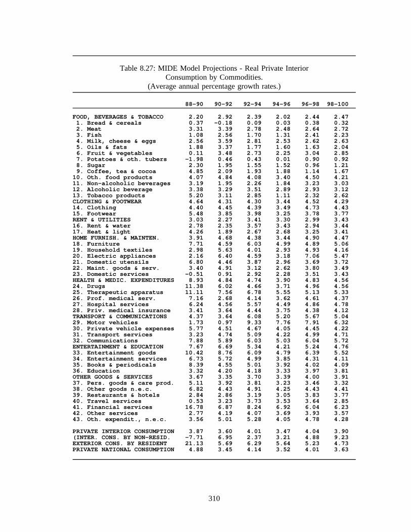
Table 8.27: MIDE Model Projections - Real Private InteriorConsumption by Commodities.
(Average annual percentage growth rates.)
88-90 90-92 92-94 94-96 96-98 98-100
FOOD, BEVERAGES & TOBACCO 2.20 2.92 2.39 2.02 2.44 2.471. Bread & cereals 0.37 -0.18 0.09 0.03 0.38 0.322. Meat 3.31 3.39 2.78 2.48 2.64 2.723. Fish 1.08 2.56 1.70 1.31 2.41 2.234. Milk, cheese & eggs 2.56 3.59 2.81 2.53 2.62 2.635. Oils & fats 1.88 3.37 1.77 1.60 1.63 2.046. Fruit & vegetables 0.11 3.48 2.73 2.25 3.04 2.857. Potatoes & oth. tubers -1.98 0.46 0.43 0.01 0.90 0.928. Sugar 2.30 1.95 1.55 1.52 0.96 1.219. Coffee, tea & cocoa 4.85 2.09 1.93 1.88 1.14 1.67
10. Oth. food products 4.07 4.84 4.08 3.40 4.50 4.2111. Non-alcoholic beverages 3.19 1.95 2.26 1.84 3.23 3.0312. Alcoholic beverage 3.38 3.29 3.51 2.89 2.93 3.1213. Tobacco products 5.20 3.11 2.85 1.11 2.32 2.62CLOTHING & FOOTWEAR 4.64 4.31 4.30 3.44 4.52 4.2914. Clothing 4.40 4.45 4.39 3.49 4.73 4.4315. Footwear 5.48 3.85 3.98 3.25 3.78 3.77RENT & UTILITIES 3.03 2.27 3.41 3.30 2.99 3.4316. Rent & water 2.78 2.35 3.57 3.43 2.94 3.4417. Heat & light 4.26 1.89 2.67 2.68 3.25 3.41HOME FURNISH. & MAINTEN. 3.91 4.68 4.38 3.44 4.90 4.4718. Furniture 7.71 4.59 6.03 4.99 4.89 5.0619. Household textiles 2.98 5.63 4.01 2.93 4.93 4.1620. Electric appliances 2.16 6.40 4.59 3.18 7.06 5.4721. Domestic utensils 6.80 4.46 3.87 2.96 3.69 3.7222. Maint. goods & serv. 3.40 4.91 3.12 2.62 3.80 3.4923. Domestic services -0.51 0.91 2.92 2.28 3.51 3.43HEALTH & MEDIC. EXPENDITURES 8.93 4.84 4.74 3.90 4.83 4.5624. Drugs 11.38 6.02 4.66 3.71 4.96 4.5625. Therapeutic apparatus 11.11 7.56 6.78 5.55 5.13 5.3326. Prof. medical serv. 7.16 2.68 4.14 3.62 4.61 4.3727. Hospital services 6.24 4.56 5.57 4.49 4.86 4.7828. Priv. medical insurance 3.41 3.64 4.44 3.75 4.38 4.12TRANSPORT & COMMUNICATIONS 4.37 3.64 6.08 5.20 5.67 5.0429. Motor vehicles 1.73 0.97 9.33 7.76 7.91 6.3230. Private vehicle expenses 5.77 4.51 4.67 4.05 4.45 4.2231. Transport services 3.23 4.74 5.09 4.22 4.99 4.7132. Communications 7.88 5.89 6.03 5.03 6.04 5.72ENTERTAINMENT & EDUCATION 7.67 6.69 5.34 4.21 5.24 4.7633. Entertainment goods 10.42 8.76 6.09 4.79 6.39 5.5234. Entertainment services 6.73 5.72 4.99 3.85 4.31 4.1135. Books & periodicals 8.39 4.55 5.01 3.92 4.02 4.0936. Education 3.32 4.20 4.18 3.33 3.97 3.81OTHER GOODS & SERVICES 3.67 3.35 3.70 3.39 4.00 3.9137. Pers. goods & care prod. 5.11 3.92 3.81 3.23 3.46 3.3238. Other goods n.e.c. 6.82 4.43 4.91 4.25 4.43 4.4139. Restaurants & hotels 2.84 2.86 3.19 3.05 3.83 3.7740. Travel services 0.53 3.23 3.73 3.53 3.64 2.8541. Financial services 16.78 6.87 8.24 6.92 6.04 6.2342. Other services 2.77 4.19 4.07 3.69 3.93 3.5743. Oth. expendit., n.e.c. 3.56 5.01 5.28 4.05 4.78 4.28
PRIVATE INTERIOR CONSUMPTION 3.87 3.60 4.01 3.47 4.04 3.90(INTER. CONS. BY NON-RESID. -7.71 6.95 2.37 3.21 4.88 9.23EXTERIOR CONS. BY RESIDENT 21.13 5.69 6.29 5.64 5.23 4.73PRIVATE NATIONAL CONSUMPTION 4.88 3.45 4.14 3.52 4.01 3.63
310

Table 8.28: MIDE Model Projections - Consumption Prices by Commodity.(Average annual percentage growth rates.)
88-90 90-92 92-94 94-96 96-98 98-100
FOOD, BEVERAGES & TOBACCO 7.06 4.10 4.08 3.36 2.51 2.391. Bread & cereals 8.10 7.52 4.16 2.96 2.29 2.332. Meat 4.74 3.21 4.15 2.94 2.41 2.293. Fish 6.56 4.72 4.15 2.97 2.29 2.324. Milk, cheese & eggs 6.66 2.80 4.19 3.04 2.43 2.405. Oils & fats 10.08 -1.70 4.16 2.96 2.29 2.346. Fruit & vegetables 11.01 4.35 3.68 2.61 2.22 2.137. Potatoes & oth. tubers 15.72 5.89 3.69 2.61 2.22 2.128. Sugar 1.66 3.17 4.13 2.98 2.31 2.319. Coffee, tea & cocoa -1.03 2.22 4.14 2.99 2.29 2.31
10. Oth. food products 3.75 4.56 4.16 2.97 2.30 2.3211. Non-alcoholic beverages 7.59 7.22 3.44 3.34 1.97 1.9412. Alcoholic beverage 12.18 5.57 3.45 3.34 1.96 1.9413. Tobacco products 5.26 6.48 5.98 12.40 5.46 4.47CLOTHING AND FOOTWEAR 5.04 5.17 3.52 3.14 2.25 2.5414. Clothing 5.22 5.15 3.37 3.06 2.21 2.5315. Footwear 4.47 5.20 4.13 3.45 2.31 2.57RENT & UTILITIES 7.37 6.45 3.84 2.53 1.95 1.4616. Rent and water 7.84 5.45 3.26 2.47 1.34 1.3017. Heat & light 5.36 9.97 5.84 3.01 3.61 1.90HOME FURNISH. & MAINTEN. 5.36 5.33 3.77 3.26 2.44 2.8618. Furniture 5.98 6.05 3.87 3.27 2.85 3.0019. Household textiles 3.98 4.57 3.42 3.02 2.17 2.4420. Electric appliances 3.17 4.05 3.36 2.93 2.01 2.5521. Domestic utensils 3.90 4.92 3.99 3.43 2.56 2.8622. Maint. goods & serv. 3.85 3.97 3.70 3.14 2.18 2.5223. Domestic services 11.23 9.53 4.75 4.20 3.90 4.43HEALTH & MEDIC. EXPENDITURES 4.53 7.00 4.95 3.99 3.19 3.4624. Drugs 0.51 3.10 3.50 3.02 2.05 2.4325. Therapeutic apparatus 1.00 2.87 3.37 2.77 2.33 2.5126. Prof. medical serv. 8.20 10.81 6.20 4.78 4.12 4.2427. Hospital services 9.17 10.84 6.19 4.78 4.11 4.2428. Priv. medical insurance 10.65 10.90 5.93 4.56 3.90 4.07TRANSPORT & COMMUNICATIONS 6.79 6.63 3.49 2.10 2.39 2.5829. Motor vehicles 5.79 4.87 1.89 -0.56 1.41 2.1430. Private vehicle expenses 8.81 7.00 4.27 3.34 2.97 2.9831. Transport services 5.47 8.45 4.43 3.26 3.24 3.0932. Communications 1.82 7.49 2.27 2.29 1.38 1.38ENTERTAINMENT & EDUCATION 4.36 5.65 4.88 4.06 3.31 3.6833. Entertainment goods 0.52 2.79 3.69 3.06 2.48 2.9734. Entertainment services 6.77 8.44 6.53 5.22 4.55 4.5035. Books & periodicals 8.41 5.72 2.67 3.62 2.69 3.9336. Education 7.27 8.78 6.55 5.06 4.62 4.58OTHER GOODS & SERVICES 8.64 9.15 5.98 4.74 4.10 4.0837. Pers. goods & care prod. 5.66 8.10 5.96 5.11 4.18 4.5838. Other goods n.e.c. 5.38 5.56 4.28 3.33 2.75 3.0539. Restaurants & hotels 9.59 8.65 4.68 3.21 2.80 2.0940. Travel services 10.43 8.48 4.15 2.71 2.93 3.6241. Financial services 7.11 7.69 4.52 3.38 2.53 3.0842. Other services 7.11 7.30 5.20 3.87 3.06 3.3643. Oth. expendit., n.e.c. 8.51 10.17 7.50 6.30 5.38 5.73
PRIVATE INTERIOR CONSUMPTION 6.65 6.26 4.12 3.08 2.59 2.54(INTER. CONS. BY NON-RESID.) 7.12 6.34 3.96 2.87 2.32 2.26EXTERIOR CONS. BY RESIDENTS 2.19 0.82 1.04 1.42 1.16 4.06PRIVATE NATIONAL CONSUMPTION 6.67 6.15 4.09 3.09 2.57 2.54
311

Table 8.29: MIDE Model Projections - Fixed Capital Investment.(Average annual percentage growth rates.)
88-90 90-92 92-94 94-96 96-98 98-100
AGRICULTURAL PRODUCTS -0.43 1.85 0.34 0.84 -0.82 -0.20
METAL PRODUCTS & MACHINERY 7.02 1.11 3.93 4.21 5.13 4.722. Metal products 5.52 1.37 2.52 2.88 3.29 2.973. Agricultural machinery -0.94 -1.21 2.60 10.59 11.76 8.044. Industrial machinery 9.27 0.44 2.57 5.58 5.07 5.415. Office mach. & computers 7.58 1.65 5.31 4.28 5.31 4.506. Elect. & electronic mach. 6.06 1.73 5.78 2.78 5.41 4.58
TRANSPORT EQUIPMENT 8.55 1.90 4.18 4.40 4.40 4.707. Automotive vehicles 8.01 2.25 2.75 3.35 4.56 4.228. Other Transport equipment 12.20 -0.24 13.61 10.16 3.61 7.10
RESIDENTIAL CONSTRUCTION 5.35 -3.68 3.85 3.79 4.87 3.94
NON-RESIDENTIAL CONSTRUCTION 18.78 6.96 4.00 5.04 4.68 5.02
OTHER PRODUCTS 2.80 0.57 5.59 4.66 4.03 2.50
FIXED CAPITAL INVESTMENT 10.93 2.69 4.02 4.54 4.75 4.63
Table 8.30: MIDE Model Projections - Prices of Fixed Capital Investment.(Average annual percentage growth rates.)
88-90 90-92 92-94 94-96 96-98 98-100
AGRICULTURAL PRODUCTS -3.20 1.02 3.45 2.46 2.21 2.14
METAL PRODUCTS & MACHINERY 3.50 2.40 2.22 2.63 1.84 2.802. Metal products 3.08 4.71 3.75 3.55 2.66 3.133. Agricultural machinery 6.30 2.07 2.15 2.21 1.68 2.544. Industrial machinery 3.24 2.07 2.14 2.23 1.68 2.565. Office mach. & computers 3.97 2.40 1.63 2.27 1.72 2.446. Elect. & electronic mach. 3.22 1.63 2.01 2.60 1.70 3.13
TRANSPORT EQUIPMENT 2.93 1.60 2.17 1.82 1.63 2.617. Automotive vehicles 2.33 1.49 1.55 1.65 1.25 2.088. Other Transport equipment 6.12 2.67 3.64 1.40 3.25 4.01
RESIDENTIAL CONSTRUCTION 6.75 6.25 4.63 3.54 2.94 3.13
NON-RESIDENTIAL CONSTRUCTION 6.76 5.64 4.36 3.42 2.87 3.04
OTHER PRODUCTS 5.36 3.19 3.27 2.98 3.01 3.32
FIXED CAPITAL INVESTMENT 5.70 4.98 4.03 3.39 2.89 3.15
312

CHAPTER 9:
CONCLUSIONS AND DIRECTIONS FOR FURTHER WORK
The purpose of this dissertation was to develop and apply a dynamic, macroeconomic,
multisectoral model of the Spanish economy. Combining the classical input-output
formulation with extensive use of regression analysis, the Modelo Macroeconómico
Intersectorial de España (MIDE) employs a "bottom-up" approach to modeling. In this
approach the macroeconomic quantities are determined by summing up individually modeled
sectoral and commodity level results. The bottom-up, disaggregated characteristic of the
MIDE model enables it to provide a much richer description of the economy than other
existing models of Spain. Other characteristics of the model include:
1) An aggregate consumption function which smoothes the effects of changes inincome. It also integrates a wealth effect designed to stifle demand duringperiods of high inflation. Increases in unemployment also dampen demand.A system of consumption functions allocate total private consumption among43 categories of goods.
2) Investment accelerator functions which respond to activity in the investingindustries, relative investment to production prices, and monetary conditions.
3) Export equations which depend on demand conditions in Spain’s tradingpartner countries, relative prices and exchange rates. Similarly, the importfunctions depend on domestic demand and the relative price of imports todomestic production.
4) Sectoral potential output which is modeled with essentially exogenousproductivity trends.
5) A wage function which responds to recent inflation and the gap betweenunemployment and the "natural rate of unemployment".
6) Sectoral profit functions which respond to wage costs and, for tradeablegoods industries, international prices and tariff rates.
313
The addition of the MIDE model to the small inventory of empirical models of Spain is
particularly timely. The MIDE model is the only multisectoral, dynamic, macroeconomic
model of the Spanish economy with significant (i.e., over twelve sectors) disaggregation.
Therefore, it can be used for applications where other, existing models are inadequate.
The most important influence on the course of the Spanish economy for the next decade
will be the continuing integration of the EC. The Europe 1992 program will eliminate all
barriers to trade, capital and labor movements between the Community countries. Many
people feel that Spain will not be capable of competing in this market and unemployment,
the most serious problem in Spain, will increase with the arrival of the single market.
Another EC issue troubling to Spaniards is the prospect of meeting the convergence criteria
in preparation for European monetary union. The recent Convergence Plan outlined by the
government makes it clear that substantial labor market and government budgetary reforms
will have to be made.
The MIDE model, as a comprehensive and detailed representation of the Spanish
economy, is a convenient tool for investigating the impact of EC integration. In this work,
the MIDE model provided individual assessments of the effects of the elimination of border
controls, the opening of public procurement contracts, financial liberalization, changes in
producer behavior and fiscal harmonization. It also provided an evaluation of the total
impact of the single market integrating all of the above aspects of integration. The results
demonstrate that with successful adaptation to the single market, governmental budgetary
restraint, wage moderation and some luck in export markets, the Spanish economy can
approach "monetary convergence" with the rest of the EC. Moreover, convergence can be
accomplished without suffering significant decreases in the growth of income and
314

employment. Finally, the model’s detailed industry-level projections illustrate a maturing
economy becoming even more integrated in the international economy.
MIDE, as any large scale empirical model, is in a continuous state of development.
Moreover, the data base is constantly being improved as new information becomes available.
One direction for future work involves the installation of the 1986 input-output table as the
base of the model. In addition to the advantages of integrating more recent economic
structure of the economy into the model, basing the model on the 1986 table will simplify
the data compilation tasks required to maintain the model, because the current version of the
national accounts are use this table as a benchmark. Moreover, the table is more
disaggregated, consisting of 56 sectors, as opposed to the current 43 of the MIDE model.
Another interesting project is the separation of the sectoral import functions of the
model by source between the EC and the Rest of the world. The same will be done for
sectoral exports, according to destination. Since the price relationships of the two
geographic areas will be very different in the future, I expect that this will enhance the
model’s foreign trade predictive capabilities.
Finally, the most important direction for future work should address what I consider to
be the weakest aspect of the present MIDE model. That is, the relationship between
investment, capital stock, potential output and prices. While it is relatively easy to specify
a relationship between conditions in the labor market and prices (the unemployment rate has
a negative relationship with wages, and wages feed into prices), due to the lack of data on
investment purchases by sector, capital capacity constraints cannot be directly modeled on
the sectoral level. The current formulation posits that rapid increases in sectoral output
signal high capacity utilization which translate into higher sectoral profits. Higher profits
lead to higher prices, mitigating demand increases and stabilizing the economy. This
315

"proxy" variable approach can clearly be improved on. Moreover, industry capital stocks
can be made to depend on investment in order to make the determination of potential output
endogenous.
There are several different possibilities for accomplishing this task. One scheme could
make the profits depend positively on the capital-output ratio. Another would be to
construct full-blown production functions to project labor and capital requirements. This
would add an endogenous component to the determination of labor productivity. It would
also change the way MIDE determines investment. However, any satisfactory solution
depends on the acquisition of data on disaggregated investment purchases. The recent
appearance of this type of data in the Bank of Spain’s central balances could make the
project feasible.
The Spanish economy will continue to grow and change in the years to come. This
growth and change will be different across sectors of the economy. Macroeconomic,
multisectoral models are designed to describe the impacts on individual sectors of the
economy in the midst of macroeconomic change. Since MIDE provides long term forecasts
in a comprehensive and integrated framework, it can play an important role in analyzing
questions confronting economists, government and business planners.
316

APPENDIX: THE DATA BASE OF THE MIDE MODEL
The foundation of the MIDE model is the 1980 Input-Output table with 43 sectors
(TIO80), constructed by the Instituto Nacional de Estadística (INE). The national accounts
(Contabilidad Nacional de España or CNE), also compiled by the INE, provide the
macroeconomic quantities of the model (with the exception of money supply, interest rates
and exchange rates which come from the Banco de España, and employment, which comes
form a separate survey.) To construct the model as outlined in this work, times series on
output, investment sales, inventory change, exports, imports, prices, income (value added)
and employment for each of the input-output (IO) sectors are required. In addition, I needed
private consumption expenditures in as much product detail as possible. The national
accounts provides sectoral-level, times series data for outputs, value added, consumption and
investment. Although the availability of this data varies, the national accounts served as the
initial source and benchmark for the compilation of data for these variables. Sectoral data
for inventory change, imports, exports, employment and output prices had to be constructed
from other sources.
Since 1954, disruptions in the homogeneity of the national accounts have occurred five
times. These revisions were made by INE so the national accounts would conform more
fully to the European System of Integrated Economic Accounts (SEC). Consequently, I had
three different sets of national accounts data covering three different periods. The first set
of accounts, labelled CN70 since its constant-price quantities appear in 1970 prices, covers
the period of 1954 through 1982.11 The second set, the CN80 accounts, presents data for
11 The 1964-69 data of this set of national accounts was itself compiled from the earliernational accounts based in 1964 (CN64). However, since INE published all the data of theseyears according to the CN70 definitions, we need not be concerned with this technicality.
317

1980 through 1988. Its constant-price quantities are expressed in 1980 prices. Finally, a
third set of national accounts, CN86, provides data for the period of 1985 through 1991.
The MIDE model is based on the CN80 accounts since they are benchmarked to the 1980
input-output table.
The national account revisions involved modifications in both the coverage and
definitions of the data. The "coverage" of a data series changes when the magnitude of a
variable with the same definition would be different in the same period when it is measured
by the different accounting schemes. For instance, the current value GDP reported by the
CN70 accounts for 1980 differs from the 1980 figure in the CN80 accounts. Such
differences between overlapping data points occurs from changes in data collection or
accounts reconciliation methodology. A more serious heterogeneity occurs when the
variable definitions change between the accounting schemes. For example, virtually all of
the sectoral classifications for disaggregated variables changed between the CN70 and CN80
accounts.
Often, the revisions presented severe compatibility problems between the data of
different accounts. In order to construct times series of data covering any reasonable
interval for regression purposes, it was necessary to homogenize the other two sets of data
to the CN80 based accounts. The homogenization between the CN80 and CN86 data was
particularly important. Without linking the most current data, historical simulations of the
MIDE model could not be verified adequately, and forecasts could not use all the
information currently available. The Ministerio de Economía y Hacienda partly solved the
linkage problem by constructing homogeneous CN80 series from the CN70 data for 1954
The original source of the 1954-63 data was the CN58 based national accounts. This washomogenized with the CN70 accounts by Uriel (1986).
318

through 1979 for the principal aggregates (Corrales and Taguas, 1989). Not only did the
provision of this data reduce my data revision workload, it provided a general technique for
linking the remaining CN70 data and the CN86 data with the CN80 accounts.12
This technique takes a "top-down" approach to homogenization, starting with the Gross
domestic product. Nominal GDP from different accounts is linked with the following
transformation:
X 80t X 70
t
X 8080
X 7080
where is GDP in current prices for year t in the CN80, and is GDP in currentX 80t X 70
t
prices for year t in the CN70 accounts. (For the CN86 to CN80 linkage, the 70 would be
replace by 86.) The equation simply multiplies the series of the linked accounts (CN70) by
the ratio between the two values in the base year (1980) of the base account (CN80).
Identically, GDP in constant prices is linked using:
KX 80t KX 70
t
KX 8080
KX 7080
where the "K" preceding the variable signifies constant prices. This technique has the
advantage of preserving the rate of growth of GDP, for both the current and constant price
values, as stated in the original published data. Transforming the components of GDP
(consumption, investment, imports, etc.) in the identical manner, however, produces series
which will not sum to the new GDP figure. Therefore, some type of scaling must be used
12 There are several technical considerations, and some subjectivity, involved inperforming this type of data homogenization. Rather than detail these here, I refer the readerto Corrales and Taguas (pp. 21-28).
319

to guarantee that the sum of the computed components add up to GDP. The best way is to
apportion the difference between the sum of the new components and the new value of GDP
using the relative weight of each component. While this technique will not guarantee that
the growth rate of each component in the new base will be equal to its growth rate in the
old base, their differences will be minimized. The linkage and scaling is accomplished
simultaneously by the equation:
X 80i,t X 70
i,t
X 80i,80
X 70i,80
X 80t
n
i
X 70i,t
X 80i,80
X 70i,80
where are the n components of GDP in year t and CN base b.X bi,t ;i 1,n
The process was repeated for constant price values of the GDP components. The
components of each GDP component were homogenized similarly. For example, fixed
investment in equipment, transport machinery, residential construction and non-residential
construction are linked using the total fixed investment calculated above as the control.
This technique was satisfactory when the definitions and the degree of aggregation for
each data series is equivalent between the bases, as is normally the case for macroeconomic
quantities and between the CN80 and CN86 sectoral data. The homogenization problem was
particularly troublesome with the CN70 to CN80 sectoral linkages because: 1) the level of
aggregation and sectoral definitions had changed between the two accounts, and 2) there was
no overlapping data for several items which did not appear in the published CN70 accounts
after 1977 or 1978.
The general approach for homogenizing the CN70 and CN80 accounts for any given
set of variables, say private consumption by commodities, was to apply the proportional
320

scaling technique when sectoral definitions were equivalent. Where sectoral definitions were
changed, I used special techniques and simplifying assumptions for an individual or group
of sectors, and often used other data from outside the national accounts. The resulting
sectoral time series follow the definitions and disaggregation provided by the CN80 and sum
to the homogeneous macroeconomic data provided by Corrales and Taguas. Since the major
purpose of these pre-1980 data is the estimation of the behavioral equations of the model,
I ultimately judged their quality and consistency by their usefulness in these equations. If
the data yield sensible estimates of parameters for the model, without evidence of
heterogeneity in the sample, they are considered usable.
Furthermore, the data was extensively evaluated against other available data, such as
raw production, consumption or foreign trade statistics. For example, constant price
production of the coal industry is compared to tons of coal produced, or tons of meat
produced is compared against the constant price value of meat consumed (foreign trade
being negligible). Generally, these comparisons were favorable. Sometimes, unfavorable
comparisons of this type led to revisions of the data. More often than not, however, there
was little alternative to the calculated series. While conserving the computed series, a note
was made indicating that it was unreliable. The text of this dissertation is sprinkled with
examples where known data problems for a particular variable resulted in the modification
of the regression intervals or standard estimation methods. With these opening comments
out of the way, I now move to discuss the compilation of the data base by each type of
sectoral series.13
13 Further details of the problems presented by, and the techniques used for the linkageof the sectoral level variables between the CN70 and the CN80 are presented in Sanz (1990).The most specific information is contained in various internal documents and programmingcode of the Fundación Tomillo, which can be provided by request.
321

Real private interior consumption and prices by commodity (43 commodities)
Real Consumption: 1964-89Prices: 1964-89Original data sources:- INE (1991b) CN86.- INE (1988) CN80.- INE (1982a) CN70.- INE (various years) Indices de Precios de Consumo (IPC).
Three serious compatibility problems existed between the CN70 data with the CN80
data. First, the commodity level data from 1964 through 1979 is compiled by Private
national consumption (i.e. inclusive of resident consumption outside the country and
exclusive of nonresident consumption inside the country.) Second, the commodity
definitions were different and the level of disaggregation was lower for the CN70 data.
From 1964 through 1977, consumption in the CN70 was published in constant and current
prices for nine major product categories and 30 sub-categories (not 43 as in CN80). There
is little or no detail under major functions 3 (Rents and utilities), 4 (Furniture and articles
for the home) and 5 (Drugs, medical services and health goods). Finally, for the years 1978
and 1979, data covering only the nine major product categories were published.
The first step was to convert the CN70 nine major product categories to interior
consumption. This conversion was done with the aid of unpublished data provided by the
INE which indicated the content of the tourism consumption in each of the nine categories.
The series were then homogenized, using the proportional scaling technique explained above,
to the CN80 data for both the real and nominal values. These major categories formed two
groups. For one group, there was no further detail available in the CN70. The second
group contained further detail more or less compatible with the CN80 defined commodities.
For the first group, the detailed real commodity consumption data was simply
apportioned to the CN80 definitions using the 1980 share of the major category. Where
322

possible, a new deflator for each of these commodities was computed using the published
private consumption index (IPC). For the second group, the missing constant price
consumption detail for 1978 and 79 was determined by allocating the total for their major
group according to their 1980 proportions. The deflators for these years were determined
for each good using the published consumption price indices. The pre-1978 CN70 detailed
commodity data was then linked to the resulting 1978 figure and scaled to the major
category total, for both current and constant price amounts. Dividing the results yielded the
deflator. Each of these detailed commodities either corresponded directly to a CN80
commodity or required further disaggregation. These final disaggregations were conducted
using the 1980 proportions.
The linkage of the CN86 data, for the years 1987 through 1989 did not require such
manipulations since, mercifully, the commodity definitions are the same. In fact there was
little difference between data points in overlapping years. The standard homogenization
procedure worked fine.
323

Constant price consumption by IO sector (43 IO sectors)
Real Consumption: 1964-89Original data sources:- INE (1983a) Encuesta de Presupuestos Familiares, 1980-1981.- INE (1986) TIO80.
To compute these series, I simply multiplied the base year bridge matrix by the
consumption series by commodity for each year. The bridge matrix displays the proportion
of consumption sold by input-output (IO) category (listed in the rows) to each of the private
interior consumption categories (listed in the columns). It was computed by using the 1980-
81 budget survey which contained private consumption at a very detailed level of
aggregation. By using the correspondence (listed in the national accounts) between these
products and the IO sectors, the 43 level commodity consumption was allocated to the IO
sectors using the IO table total consumption by sector and the 1980 commodity consumption
as row and column controls, respectively. Dividing the flows in each of the cells by the
sum of the column produces the consumption coefficients applicable for each year.
Constant price output and output deflators (43 IO sectors)
Constant price output and price deflators by sector are the two most important series
of any multisectoral model. Current price production for each of the input-output (IO)
sectors is available from the national accounts from 1980 through 1985 (CN80). As
presented in the national accounts, this figure is the sum of inputs (i.e., the sum down the
column of the IO table). To arrive at this figure, INE uses either a direct measure of sales
for a given industry or a measure of total value added and intermediate purchases of the
industry. In general, value added for each industry is known through various annual
324

surveys. For agriculture and industry, surveys are conducted which provide estimates for
all three figures: production, value added and intermediate purchases. As we shall see,
however, annual data for service sectors is often incomplete and some simple assumptions
must be made to complete the national accounts.
CN86 data, though available for 1986 and 1987, was not compatible with the CN80
data because of complications arising from the introduction of the Value Added Tax in that
year. Therefore, it was often not used. Because of the absence, in the national accounts,
of any current price production series previous to 1980 and after 1985, and of any constant
price production or price series, the availability of this data was a serious problem. It was
necessary to seek out data from other sources. This necessitated a heterogeneous approach
to the output data across sectors.
Sector 1: Agriculture, forestry and fisheries
Real Output: 1964-90Prices: 1964-90Original data sources:- Ministerio de Agricultura (various years) Cuentas del sector agrario.- INE (various years) Anuario Estadístico.- INE (1991b) CN86.- INE (1988) CN80.- INE (1986) TIO80.
Gross current price production for the agriculture, forestry and fishery industries are
published by the Ministry of Agriculture and Fishing (MAPA). The sum of these production
figures forms the basis of the national account (CN) and input-output table current price
output published by INE for 1980 to 1985. By linking the MAPA figures from 1964 and
through 1990 with the CN data, I obtained current price production for all the years. MAPA
also publishes a producer’s price for the combined agricultural and forestry industries and
325

a figure for the tons of fish landed by the fisheries industry. From the latter, a crude price
index for the fisheries industry was constructed and combined with the former, using 1980
output weights, to yield the sectoral deflator. Finally, 1980 constant price production was
obtained by dividing the current price production by the deflator.
Sectors 2-25: Industry (Energy, Mining and Manufacturing)
Output: 1964(70)-91Prices: 1970-91Original data sources:- INE (various years) Anuario Estadístico.- INE (1991b) CN86.- INE (1988) CN80.- INE (1986) TIO80.- INE (various years) Indices de Precios Industriales, 1974-91.- INE (various years) Indices de Produción Industriales, 1972-91.
Official industrial price indexes for the years 1974 through 1990 are available in the
CNAE sectoring scheme (the Spanish equivalent of the U.S. Standard Industrial
Classification or SIC) at a high level of disaggregation (four digit). This enabled the
construction of appropriate output deflators for each of the industrial sectors. These
deflators were "backcasted" to 1970 with regressions of the deflators on the CN70 value-
added deflators for each of the sectors. The CN80 current price outputs were then deflated
by these indices to obtain constant price outputs for 1980-1985.
Official industrial production indexes are available from 1972 to 1990 at the four digit
level of disaggregation and back to 1964 at the two digit level. The annual rates of growth
of the appropriate production indices for each sector were then used to extend series
backward from 1980 and forward to 1991. Since most of the MIDE industries correspond
directly to two digit CNAE categories, the new series extend backward to 1964. For the
326

few industries where this was not the case, the appropriate production indices were
backcasted to 1970 by regressing the detailed index on its corresponding two digit index.
Sector 26: Construction
Real Output: 1964-91Prices: 1970-91Original data sources:- SEOPAN (various) Informe Anual Sobre la Construcción.- INE (1991b) CN86.- INE (1988) CN80.- INE, (1986) TIO80.
A construction price index compiled by the National Association of Construction Firms
(SEOPAN) extends back to 1970. The current price production figures of the national
accounts for 1980 through 1987 were deflated with this index. Since the resulting output
series was highly correlated (.996) with the national accounts constant price construction
investment total, output for 1964-1979 and 1988-91 was moved with this series.
Sectors 27: Reconstruction and RepairSector 28: Wholesale and Retail Trade
Real Output: 1964-89Prices: 1964-89Original data sources:- INE (1991b) CN86.- INE (1988) CN80.- INE (1986) TIO80.
The first item to note concerning these two sectors is that even though the TIO80
published them as two distinct sectors, the CN80 accounts reported their production and
value added data together. Therefore, it was convenient to treat any extrapolation of its
production data together, and then separate it with some criteria. A second matter of interest
is that in the CN80, the ratio of total value added to production is constant. I cannot be sure
327

why this is, but I assume that the only data available to INE was the value added data. In
the absence of total revenue or intermediate input data, INE was forced to make this
simplification. For the extrapolation of current price production I adopted this assumption.
Therefore, current price value added for the combined sector was extrapolated backward
to 1964 (CN70) and forward to 1988 (CN86) using the general homogenization technique
outlined above. The current price production was then imputed at the constant ratio implied
by the TIO80. In order to deflate this quantity, I constructed a homogenous value added
deflator from the three sets of national accounts. To split the resulting output between the
two sectors, I used the proportions implied by the consumption by IO sector. I used the IO
consumption values as independent variables in regressions to extend real output through
1989. The prices are extended through 1989 with regression using the aggregate services
value added deflator.
Sector 29: Hotels, restaurants and barsSector 36: Commercial and residential rentsSector 38: Private health ServicesSector 39: Recreation, cultural, other personal servicesSector 37: Private educationSector 43: Domestic and other non-market services
Real Output: 1964-89Prices: 1964-89Original data sources:- INE (1991b) CN86.- INE (1988) CN80.- INE (1986) TIO80.- INE (various years) Indices de Precios de Consumo (IPC).
The large majority of demand for each of these sectors is private consumption and
foreign trade is either nonexistent or trivial. In addition, each of these production sectors
have close correspondences to individual private consumption categories. Therefore, the
328

single best deflator to use in each case is the corresponding private consumption deflator.
The current price production figures of the national accounts for 1980 through 1987 are
deflated with this index. Since the resulting production is highly correlated with the private
interior consumption for each of the sectors output for 1964-1979 and 1988-90 is moved
with these series.
Sector 30: Interior transportation services (railroads, busses, subways, highway transport)Sector 31: Maritime and air transportSector 32: Other transport services (ports, airports, shipping)Sector 33: Communication
Real Output: 1964-91Prices: 1964-91Original data sources:- Ministerio de Transportes, Turismo y Comunicaciones (1989).- INE (various) Boletín Trimestral de Coyuntura.- INE (1991b) CN86.- INE (1988) CN80.- INE (1986) TIO80.- INE (various years) Anuario Estadístico.
For Interior transport, Maritime and Air transport and Communications, output and price
indices were constructed with various revenue and raw production statistics. For example,
the sum of the revenues of the government telephone and post corporations tracked very
satisfactorily with the national accounts version of nominal production of the
communications sector. I linked this revenue series to the CN data. A price deflator was
formed by dividing the specific revenue series with corresponding output statistics. For
example, a telephone price is computed by dividing the revenue of the telephone monopoly
with the number of telephone calls, telegrams, etc. for each year. The constant-price output
series is determined by moving the IO table output with weighted output indices of
telephone calls, letters, etc. The resulting series were check against various value added data
329

from the national accounts, and adjustments were made when large discrepancies were
evident.
Transport output indices were constructed with the help of similar indices compiled by
the INE using data from the Ministry of Transport. Prices for the same sectors were either
compiled from raw output and revenue data or using indices published by the Ministry of
Transport.
The current price production for Other transport services, sector 32, relied primarily on
value added data. The price index for the sector was constructed from the indices of the
other transport sectors with a regression equation.
Sector 34: Banking and InsuranceSector 40: Public AdministrationSector 42: Public educationSector 43: Public health services
Real Output: 1964-91Prices: 1964-91Original data sources:- INE (1991b) CN86.- INE (1988) CN80.- INE (1986) TIO80.
Production and value added data for these sectors is very complete for all versions of
the national accounts. Therefore, the determination current price production was an easy
affair. Also, since value added is such a large proportion of output for each of these sectors,
the value added deflators from the national accounts provide reasonable production price
indices.
330

Real fixed investment expenditures and prices by commodity (11 commodities)
Real Investment 1954-90Prices: 1964-90Original data sources:- INE (1991b) CN86.- INE (1988) CN80.- INE (1986) TIO80.- Corrales and Taguas (1988).
The investment classification corresponds to the CN80 definitions. The accounts
provide current price series from 1980 through 1990 for each of the products, and constant
price series for six categories: Agricultural products (Commodity 1), Machinery and metal
products (Commodities 2-6), Transport material (7-8), Non-residential construction (9), Other
products (10) and Residential construction (11). Data previous to 1980 exists in constant
and current prices for only four categories: Machinery and other products (1-6 and 10),
Transport material (7-8), Non-residential construction (9) and Residential construction (11).
These series have been homogenized and extended back to 1954 by Corrales and Taguas
(1989). No further compilation was required for the two construction categories.
Eight of the nine remaining commodities have a close correspondence with production
sectors of the input-output table. With the exception of category 10, Other products, each
commodity is manufactured by only one industry. This direct correspondence simplifies the
construction of a matrix which allocates the quantities demanded to the production sector
(referred to in Chapter 4 as the B matrix). However, since the investment series are in
purchaser prices, they include commercial margins, transportation costs and services
provided by five other input-output industries. To create the B matrix, these mark-ups were
allocated to the respective service sectors using information on the construction of the 1980
IO table provided by INE (see Sanz 1989).
331

The information provided by the share matrix allowed the construction of purchaser
prices for each the products using the production and import prices, weighted for the
proportion of imports in domestic demand, from the corresponding input-output sectors. The
purchaser prices were then scaled to be consistent with the available aggregate investment
deflators. Series in constant prices for each of the products were estimated for the years
previous to 1980 by using the more aggregated investment quantities and the respective
production sector domestic demand as indicators. In order to construct an estimate of the
capital stock for each of the products, it was necessary to have investment series extending
back to 1954. These were constructed by "backcasting" each series with regression
equations using the relevant aggregate constant-price series as the independent variable.
Imports and Exports (33 IO sectors)
Real Quantities: 1970-89Prices: 1970-89Original data sources:- INE (1991b) CN86, TIO87.- INE (1991c) CN86, TIO86.- INE (1988) CN80.- INE (1986) TIO80.- Dirección General de Aduanas (various) Estadística del
Comercio Exterior de España.- Banco de España (various) Boletín Estadístico.- Cañada and Carmena (1989).- Bajo and Torres (1989).
Imports and exports each have 25 merchandise categories and 8 service categories.
Current price import and export data was provided by the INE for the 56 sectors of the 1985
IO data for the years 1981 through 1987, while the 1980 data comes from the IO table. For
1970 through 1979, and 1988 through 1989, Fundación Tomillo aggregated six digit
(Brussels’ Nomenclature) merchandise trade data taken directly from the Dirección General
332

de Aduanas (Customs). Merchandise prices for the entire period and for each sector are unit
value indices also computed by Tomillo using the detailed customs data. For the same
years, current price service imports and exports were compiled from the balance of payments
accounts of the Bank of Spain and adjusted to conform with the national accounts data.
They are then deflated by their respective domestic production deflators.
Constant price values are scaled to the merchandise and service totals supplied by the
national accounts. For service imports, this scaling procedure provides new deflators which
drive a wedge between the sectoral domestic prices and the import prices in proportion to
the difference between the aggregate service domestic prices and the aggregate service
import prices. Finally, the trade and transport margins contained in merchandise exports are
allocated to the respective service sectors according to the margins indicated in the 1980
input-output table. In general, while the merchandise data is of high quality, that of services
(excluding tourism which comes directly from the national accounts) has some problems.
Fortunately, service trade comprises small shares of both aggregate trade and sectoral
outputs. A detailed description of the entire process in contained in Fierros (1990).
Industry import tax rates have been constructed by extrapolating and homogenizing the
tariff rates computed by Cañada and Carmena (1989), Bajo and Torres (1989) and the INE
in the construction of the 1980, 1986 and 1987 IO tables.
333

Inventory Change (25 merchandise IO sectors)
Real Quantities: 1970-89Original data sources:- Ministerio de Agricultura (various) Cuentas del sector agrario.- Ministerio de Industria y Energía (various) Encuesta de Opiniones Empresariales.- INE, (various) Encuesta Industrial.- INE, (1991b) CN86, TIO87.- INE, (1991c) CN86, TIO86.- INE, (1988). CN80.- INE, (1986). TIO80.
Employment (43 IO sectors)
Persons employed
Thousands of persons: 1972(76)-91Original data sources:- INE (various years) Encuesta de Población Activa.- Treadway, A. (1990b).
The Employment Survey (Encuesta de Población Activa) provides homogenous
employment series at a disaggregated level from 1976. These were used directly. The
Survey suffered a rupture in methodology before 1976. Treadway homogenized the data
from the previous Survey with the later Survey at a relatively high aggregation. For 1972-
76, employment for most of the industrial sectors was obtained using disaggregated data
from the earlier Employment Survey to disaggregated Treadway’s data. This disaggregation
was not possible for service sectors.
Hours Worked per Year
Hours: 1972-1989Original data sources:- INE (various years) Encuesta de Salarios.- Carbajo and Perea (1987).
334

The Wage Survey (Encuesta de Salarios) publishes a quarterly figure of the average
monthly hours worked for that quarter. In 1989, the Wage Survey began to publish hours
worked data at a sufficient disaggregation for MIDE’s sectoral scheme. Previous to then,
published data enumerated only 17 sectors. The collection of the data suffered several
methodological breaks, which made it difficult to compare data from different periods.
Carbajo and Perea (1987) homogenized the series to provide continuous time series from
1963 for each of the 17 sectors. In order to reach hours worked per year for each of the
MIDE sectors, I assumed that the annualized Carbajo and Perea data is the same for the
MIDE sectors covered by a single Wage Survey sector. For example, the Wage Survey
published one figure for the food processing, beverage and tobacco industries. Therefore,
the corresponding MIDE sectors (15-19) have identical series for annual hours worked per
worker.
Value Added (43 IO sectors)
Wages and SalariesGross ProfitsNet Indirect TaxesValue Added Taxes
Nominal Quantities: 1980-88Original data sources:- INE (1991b) CN86, TIO87.- INE (1991c) CN86, TIO86.- INE (1988) CN80.- INE (1986) TIO80.
These values were all taken directly from the national accounts. The homogenization
between the CN80 and CN86 accounts was straightforward because only nominal quantities
were involved.
335

Sector and Commodity Classifications of the MIDE Model
Production sectors of the Input-Output Table
1. Agriculture, forestry and fisheries2. Coal, lignite, and radioactive material3. Coke4. Crude petroleum, natural gas and refining5. Electrical, gas, steam and water utilities6. Ferrous and nonferrous minerals and metals7. Nonmetallic minerals and products8. Chemicals9. Metal products, except machinery and transport
10. Industrial and agricultural machinery11. Office machinery, computers, precision and optical instruments12. Electrical and electronic material and accessories13. Motor vehicles and engines14. Other transport material15. Meat, prepared and preserved, other animal products16. Dairy products17. Other food products18. Beverages19. Tobacco products20. Textiles and apparel21. Leather products, shoes22. Wood and wood products23. Paper and publishing24. Rubber and plastic products25. Other manufactured products26. Construction and civil engineering27. Repairs and reconstruction28. Wholesale and retail trade29. Restaurants, cafes and hotels30. Interior transport31. Maritime and air transport32. Transport services33. Communications34. Banking and insurance35. Business services36. Commercial and residential rents37. Private education and research services38. Private health services39. Recreation, cultural, personal and other services40. Public administration41. Public education services42. Public health services43. Domestic and other services n.e.c.
336

Private Interior Consumption Commodities
1. Bread and cereals2. Meat3. Fish4. Milk, cheese and eggs5. Oils and fats6. Fruits and vegetables7. Potatoes and other tubers8. Sugar9. Coffee, tea and cocoa
10. Other food products11. Nonalcoholic beverages12. Alcoholic beverages13. Tobacco products14. Clothing15. Shoes16. Rent and expenditures on water17. Heat and electricity18. Furniture and fixed
accessories, carpets19. Household textiles and
other accessories20. Household appliances21. Tableware and other
domestic utensils22. Goods and services for
household maintenance
23. Domestic services24. Drugs and other pharmaceutical
products25. Therapeutic equipment and
apparatus26. Medical services of doctors and
other professionals27. Hospital attention28. Private medical insurance premiums29. Motor vehicles30. Expenditures on motor vehicles31. Transport services32. Communication services33. Entertainment goods34. Entertainment and cultural services35. Books, newspapers and magazines36. Education37. Personal care and other
personal products38. Other products n.e.c.39. Restaurants, cafes and hotels40. Travel services41. Financial services n.e.c.42. Other financial services43. Other expenditures n.e.c.
Investment Products
1. Agricultural, forestry and fishery products2. Metal products3. Agricultural machinery and tractors4. Industrial machinery5. Office machinery, computers, precision and optical instruments6. Electrical and electronic machinery and material7. Motor vehicles8. Other transport material, including ships, planes, and railroad9. Residential construction
10. Nonresidential construction11. Other products
337

REFERENCES
Abadía, Antonio (1984). Un sistema completo de demanda para la economía española.Working Paper 8402, Fundación Empresa Pública and Universidad Complutense,Madrid.
Abadía, Antonio; Jose Borrell and Oscar Fanjul (1981). Un modelo dinámico multisectorialde crecimiento económico, empleo y redistribución del la renta (Madrid: Fundación delInstituto Nacional de Industria).
Alcaide, Carmen and T. Martínez Aguado (1990). Predicciones de la economía española1989-1992. Situación, 1990/2, pp. 105-122 (Madrid: Banco Bilbao Vizcaya).
d’Alcantara, G and A. Italianer (1982). European project for a multinational macrosectoralmodel. Report MS 11 to the Commission of the European Communities. (Brussels:Directorate-General for Science, Research and Development).
Almon, Clopper (1991). The INFORUM Approach to Interindustry Modeling. EconomicSystems Research, 3 (1), pp. 1-7.
Almon, Clopper (1989). The Craft of Economic Modeling, 2nd ed. (Needham Heights, MA:Ginn Press).
Almon, Clopper (1986). Principles and Practices of the INFORUM Interindustry MacroModel. Vierteljahrshefte zur Wirtschaftsforschung, 3, pp. 167-178 (Deutsches Institutfur Wirtschaftsforschung).
Almon, Clopper (1984). The INFORUM-IIASA International System of IO Models. InProceeding of the Seventh International Conference of Input-Output Techniques (NewYork: United Nations)
Almon, Clopper (1983). The Price-Income Block of the U.S. Inforum Model. In M. Grassiniand A. Smyshlyaev, eds. Input-Output Modelling: Proceedings of the Third IIASA TaskForce Meeting, pp. 219-236 (Laxenburg, Austria: International Institute of AppliedSystems Analysis, CP-83-S2).
Almon, Clopper (1979). A System of Consumption Functions and its Estimation forBelgium. Southern Economic Journal, 46 (July 7), pp. 85-106.
Almon, Clopper; Margaret Buckler, L.M. Horwitz and T.C. Reimbold (1974). 1985:Interindustry Forecasts of the American Economy (Lexington, MA: Lexington Books).
Almon, Clopper (1966). The American Economy to 1975 (New York: Harper and Row).
338

Andres, Javier; César Molinas and David Taguas (1990). Una función de consumo privadopara economía española: Aplicación del análisis de cointegración. Working PaperSGPE-D-90002, Ministerio de Economía y Hacienda, Dirección General dePlanificación, Madrid.
Andres, Javier; Alvaro Escribano; César Molinas and David Taguas (1989). La Inversión enEspaña: Un Enfoque Macroeconómico. Moneda y Crédito, 188, pp. 67-98.
Andres, Javier; Juan José Dolado; César Molinas; Miguel Sebastián and Antonio Zabalza(1988a). The Influence of Demand and Capital Constraints on Spanish Unemployment(Revised Version). Working Paper SGPE-D-88005, Ministerio de Economía y Hacienda,Dirección General de Planificación, Madrid.
Andres, Javier; Alvaro Escribano; César Molinas and David Taguas (1988b). Una FunciónAgregada de Inversión Productiva Para la Economía Española. Working Paper SGPE-D-88006, Ministerio de Economía y Hacienda, Dirección General de Planificación,Madrid.
Antón, Vincente and Fatima Escribano (1988). La Desagregación de la Formación BrutaCapital Fijo por Rama Propietaria: Los Coeficientes de Capital. Working Paper dt-88-04, Instituto Nacional de Estadística, Madrid.
Baiges, Josep; Cesar Molinas and Miguel Sebastián (1987). La Economía Española 1964-1985: Datos, Fuentes y Análisis (Madrid: Ministerio de Economía y Hacienda, Institutode Estudios Fiscales).
Ballabriga, F.C.; César Molinas; Miguel Sebastián and Antonio Zabalza (1990). DemandRationing and Capital Constraints in the Spanish Economy. Paper presented to the SixthWorld Congress of the Econometric Society, Barcelona.
Bajo, Oscar and Angel Torres (1989). The Determinants of Import Protection in SpanishManufacturing Industry. Mimeo. Ministerio de Economía y Hacienda, Madrid.
Baldwin, Richard (1989). The Growth Effects of 1992. Economic Policy, October.
Banco Bilbao Vizcaya (1990). Situación, 2 (Madrid: Banco Bilbao Vizcaya).
Banco de España (1991a). Cuentas Financieras de la Economía Española (1981-1990)(Madrid: GraphicasReunidas, S.A.).
Banco de España (1991b). Boletín Estadístico, (June).
Banco de España (1990). Cuentas Financieras de la Economía Española (1980-1989)(Madrid: GraphicasReunidas, S.A.).
339

Barbera, Anthony (1982). A Model of Net Investment, Replacement Investment, and LaborRequirements. IIASA Task Force Meeting on I-O Modeling, September 1982, andPh.D. dissertation, University of Maryland.
Bardazzi, Rossella; Maurizio Grassini and Ernesto Longobardi (1991) Value-Added Taxesand Other Indirect Taxes in an EEC Country Model: The Italian Case. EconomicSystems Research, 3 (1), pp. 37-47.
Barker, Terry and William Peterson, eds. (1987). The Cambridge Multisectoral DynamicModel of the British Economy (Cambridge: Cambridge University Press).
Barten, A.P. (1967). Evidence on the Slutsky Condition for Demand Operations. Review ofEconomics and Statistics, 49, pp. 77-84.
Bel i Queralt (1991). La financiación de las Comunidades Autónomas. Notebooks ofEconomics and Finance, Number 4 (Madrid: Fundación de Estudios EconomíaAplicada).
Blanchard, Olivier; Rudiger Dornbusch; Jacques Drèze; Herbert Giersch; Richard Layard andMario Monti (1985). Employment and Growth in Europe: A Two Handed Approach.Center for European Policy Studies Papers, 21.
Buigues, P.; F. Ilzkovitz and J-F. Lebrun, editors (1990). The Impact of the Internal Marketby Industrial Sector: The Challenge for the Member States. European Economy, SocialEurope, Special Edition (Brussels: Commission of the European Communities).
Cañada, Agustín and Ana Carmena (1991). Los cambios en el sistema fiscal-arancelario:repercusiones sobre la competividad española (1986-1989). Información ComercialEspañola: Boletín Económico (January 14), pp. 11-27.
Cañada, Agustín and Ana Carmena (1989). Protección de la Economía Española: UnAnálisis de la Evolución en el Periodo 1980-1986. Información Comercial Española:Boletín Económico, 2195 (August 7), pp. 3177-3189.
Carbajo, Ramón and Pilar Perea (1987) Series Históricas Homogéneas de Horas Trabajadas.Document 87-09, Fundación de Estudios Economía Aplicada, Madrid.
Carreras, Albert, editor (1989). Estadísticas históricas de España: Siglos XIX-XX (Madrid:Fundación Banco Exterior).
Casares, Javier; Pablo Muñoz and Alfonso Rebollo (1990). La distribución comercial enEspaña. Papeles de Economía Española, 42, pp. 251-61 (Madrid: Fundación Fondo parala Investigación Económica y Social).
340
Catinat, Michel and Alexander Italianer (1988). Completing the Internal Market. PrimaryMicroeconomic Effects and Their Complementation in Macro-econometric Models.Report II/140/88. Commission of the European Communities (Brussels: Directorate-General for Economic and Financial Affairs).
Catinat, Michel; Eric Donni and Alexander Italianer (1988). The Completion of the InternalMarket: Results of Macroeconomic Model Simulations. In Commission of theEuropean Communities, Research on the "Cost of Non-Europe" Studies on theEconomics of Integration, Volume 2 (Brussels).
Cecchini, Paolo and others (1988). The European Challenge 1992: The Benefits of a SingleMarket (Aldershot, England: Wildwood House for the EE Commission).
Christou, Costas and Douglas Nyhus (1992). Industrial Effects of European CommunityIntegration. Mimeo, INFORUM, University of Maryland.
Cinco Dias (1992). El programa muestra la necesidad de un pacto de rentas. April 6, p. 12.
Coe, David T. and Francesco Gagliardi (1985). Nominal Wage Determination in Ten OECDCountries. OECD Department of Economics and Statistics Working Paper, No. 19(Paris: OECD).
Commission of the European Communities (1985). Completing the Internal Market: WhitePaper from the Commission to the European Council (Luxembourg).
Corrales, Adolfo and David Taguas (1989). Series Macroeconómicas para el Periodo 1954-88: Un Intento de Homogeneización (Madrid: Ministerio de Economía y HaciendaInstituto de Estudios Fiscales).
Cowhey, Peter F. (1990). Telecommunications. In Gary Hufbauer, ed. Europe 1992: AnAmerican Perspective (Washington D.C.: Brookings Institution).
Deaton, Angus (1974). A Reconsideration of the Empirical Implications of AdditivePreferences. Economic Journal (June), pp. 338-49.
Deaton, Angus and John Muellbauer (1980). Economics and Consumer Behavior(Cambridge: Cambridge University Press).
Dervis, Kemal; Jaime de Melo and Sherman Robinson (1982). General Equilibrium Modelsfor Development Policy (Cambridge: Cambridge University Press).
Dehesa, Guillermo de la; Jose Ruiz and Angel Torres (1988). The Timing and Sequencingof a Trade Liberalization Policy: The Case of Spain. Country Manuscript (Washington:World Bank).
Diaz, Antonio (1990). Cambio Técnico de la Economía Española en el Modelo MIDE.Información Comercial Española: Revista de Economía, 683 (Julio), pp. 55-66.
341

Dirección General de Aduanas. Estadística del Comercio Exterior de España, 1970-1990.Magnetic media.
Dirección General de Planificación (1990). MOISEES: Un Modelo de Investigación ySimulación de la Economía Española. Working Paper SGPE-D-90003, Ministerio deEconomía y Hacienda, Dirección General de Planificación, Madrid.
Dones Tacero, Milagros; Fco. Javier García Sanchez and Bernardo Pena Trapero (1990). Elmodelo HERMES-España. Situación, 1990/2, pp. 79-103 (Madrid: Banco BilbaoVizcaya).
Dornbush, Rudiger (1989). Europe 1992: Macroeconomic Implications Brookings Paperson Economic Activity, 2, pp. 341-362.
The Economist (1991a). How to get good marks, or ecus. December 14, p. 30.
The Economist (1991b). Geography and geometry. In Survey of Asias’s EmergingEconomies. November 16, pp. 17-18.
The Economist (1991c). The Aid Plague. In Survey of Business in Europe. June 8, pp. 16-18.
The Economist (1991d). Pulling up the Drawbridge. In Survey of Business in Europe. June8, pp. 20-25.
The Economist (1991e). Spanish Banks: Best of the Bunch. April 26, p. 79.
El Pais (1991). Anuario El Pais 1991 (Altamira, Spain: Progresa).
Engle, R.F. and C.W.J. Granger (1987). Co-integration and Error Correction: Representation,Estimation, and Testing. Econométrica, 55, No. 2, pp. 251-276.
Eurostat (1983). European System of Integrated Economic Accounts (ESA) Second edition.
Fernández, Ismael and Miguel Sebastián (1990a). Análisis del déficit exterior. 3conomi4, 5,pp. 45-53.
Fernández, Ismael and Miguel Sebastián (1990b). Análisis del déficit exterior: el deteriorode la exportaciones en 1986 y la estabilidad de las exportaciones. Working PaperSGPE-D-90008, Ministerio de Economía y Hacienda, Dirección General dePlanificación, Madrid.
Fernández, Ismael and Miguel Sebastián (1989). El Sector Exterior y la incorporación deEspaña a la CEE: Análisis a partir de funciones de Exportaciones y Importaciones.Working Paper SGPE-D-89005, Ministerio de Economía y Hacienda, Dirección Generalde Planificación, Madrid.
342

Fernandez, P. and A. Pulido (1990). Experiencias en predicción de la economía española conel modelo Wharton-UAM. Situación, 1990/2, pp. 37-54 (Madrid: Banco BilbaoVizcaya).
Fierros, José (1990). Un análisis del sector exterior por ramas de actividad con las seriestemporales del modelo MIDE. Información Comercial Española: Revista de Economía,683 (Julio), pp. 67-91.
Ford, Robert and Pierre Poret (1991). Business Investment: Recent Performance and SomeImplications for Policy. OECD Economic Studies, 16 (Spring) pp. 79-132.
Fuentes Quintana, E. (1991). España depende en exceso de la entrada de capital. Cinco Días,12 August, p. 5.
Fuentes Quintana, E. (1989). Tres decenios de la economía española en perspectiva. In J.Garcia Delgado, ed. España: Economía, pp. 1-75 (Madrid: Espasa-Calpe SA).
Fundación Tomillo (1990). Descripción y Aplicaciones del Modelo MacroeconómicoIntersectorial de España (MIDE). Situación, 1990/2, pp. 55-77 (Madrid: Banco BilbaoVizcaya).
Gauyacq, Daniel (1985). Les Systemes Interdependants de Fonctions de Consommation.Prevision et Analyse Economique, Cahiers du Gama, 6 (June), pp 7-129.
Gonzalez-Romero, Arturo and Rafael Myro (1989). La Recuperación de la InversiónIndustrial en España (1985-1988): Sus Objetivos y Factores Determinantes. Moneda yCrédito, 188, pp. 17-55.
Grassini, Mauricio (1983). Structural Change in Italian Foreign Trade. In A. Smyshlyaev,ed. Proceedings of the Fourth IIASA Task Force Meeting on Input-Output Modeling.(Laxenburg, Austria: International Institute of Applied Systems Analysis, CP-83-5).
Holtham, G.H. and H. Kato (1986). Wealth and Inflation Effects in the AggregateConsumption Function. OECD Department of Economics and Statistics Working Paper,No. 35 (Paris: OECD).
Hooper, John (1987). The Spaniards (London: Penguin Books).
Hufbauer, Gary (1990). An Overview. In Gary Hufbauer, ed. Europe 1992: An AmericanPerspective (Washington D.C.: Brookings Institution).
Instituto Nacional de Estadística. Indices de Precios de Consumo, 1964-91. Magnetic Media.
Instituto Nacional de Estadística. Indices de Precios Industriales, 1974-91. Magnetic Media.
Instituto Nacional de Estadística. Indices de Producción Industriales, 1972-91. MagneticMedia.
343
Instituto Nacional de Estadística (various quarters). Boletín Trimestral de Coyuntura(Madrid: I.N.E. Artes Gráficas).
Instituto Nacional de Estadística (various years). Encuesta Industrial (Madrid: I.N.E. ArtesGráficas).
Instituto Nacional de Estadística (1992). Evolución de las Pricipales MagnitudesMacroeconómicas, Primeras estimación del año 1991 (Madrid: I.N.E. Artes Gráficas).
Instituto Nacional de Estadística (1991a). Anuario Estadístico 1990 (Madrid: I.N.E. ArtesGráficas).
Instituto Nacional de Estadística (1991b). Contabilidad Nacional de España, Base 1985.Serie Contable 1985-1990, Tabla Input-Output 1987 (Madrid: I.N.E. Artes Gráficas).
Instituto Nacional de Estadística (1991c). Contabilidad Nacional de España, Base 1985.Serie Contable 1985-1989, Tabla Input-Output 1986 (Madrid: I.N.E. Artes Gráficas).
Instituto Nacional de Estadística (1990a). Anuario Estadístico 1989 (Madrid: I.N.E. ArtesGráficas).
Instituto Nacional de Estadística (1990b). Encuesta de Población Activa (Madrid: I.N.E.Artes Gráficas).
Instituto Nacional de Estadística (1988). Contabilidad Nacional de España, Base 1980(Madrid: I.N.E. Artes Gráficas).
Instituto Nacional de Estadística (1987). Proyecciones de Población 1980-2010: Resultadosdel Conjunto Nacional (Madrid: I.N.E. Artes Gráficas).
Instituto Nacional de Estadística (1986). Tabla Input-Output de la Economía Española de1980 (Madrid:I.N.E. Artes Gráficas).
Instituto Nacional de Estadística (1983a). Encuesta de Presupuestos Familiares, 1980-1981(Madrid:I.N.E. Artes Gráficas).
Instituto Nacional de Estadística (1983b). Números Indices de Precios Industriales:Monografía Técnica (Madrid:I.N.E. Artes Gráficas).
Instituto Nacional de Estadística (1982a). Contabilidad Nacional de España, Base 1970(Madrid: Rivadeneyra, S.A.).
Instituto Nacional de Estadística (1982b). Números Indices de Producción Industrial:Monografía Técnica (Madrid: I.N.E. Artes Gráficas).
Instituto Nacional de Estadística (1980). Anuario Estadístico 1979 (Madrid: I.N.E. ArtesGráficas).
344

Instituto Nacional de Estadística (1977). Indices de Precios de Consumo: Estructuras de losIndices Oficiales (Madrid: I.N.E. Artes Gráficas).
Italianer, Alexander (1986). Theory and Practice of International Trade Linkage Models(Boston: Martinus Nijhoff Publishers).
Jimeno, Juan and Alberto Meixide (1991). Collective Bargaining and Wage Dynamics inSpain. Paper prepared for the ASAP Annual Conference on Earnings, Rome,November.
Kehoe, Timothy J.; Antonio Manresa; Pedro J. Noyola; Clemente Polo and Ferran Sancho(1988). A General Equilibrium Analysis of the 1986 Tax Reform in Spain. EuropeanEconomic Review, 32, pp. 1-9.
Kennedy, Peter (1985). A Guide to Econometrics, Second Edition (Cambridge: The MITPress).
Krugman, Paul (1990). The Age of Diminished Expectations (Cambridge: The MIT Press).
Lambert, P (1987). Disequilibrium Macroeconomic Models (Cambridge: CambridgeUniversity Press).
Lantero, Javier y Jeffrey F. Werling (1991). The Initial Stages of Building an INFORUMModel: the Example of Spain. Economic Systems Research, 3 (1), pp. 9-14.
Larre, Bénédicte and Raymond Torres (1991). Is Convergence a Spontaneous Process? TheExperience of Spain, Portugal and Greece. OECD Economic Studies, 16 (Spring) pp.169-198.
Lasheras, Miguel A.; Antonio de Lecea and María Antonia Monés (1989). Modelo IINDIO.Methodologia y aplicaciones. Hacienda Pública Española, pp. 19-39.
Leontief, Wassily (1986). Input-Output Economics, 2nd ed (Oxford: Oxford UniversityPress).
López Blanco, Elías and David Taguas (1990). Una visión general del modelo deinvestigación y simulación de la economía española (MOISEES). Situación, 1990/2, pp.7-35. (Madrid: Banco Bilbao Vizcaya).
Lorenzo, María José (1988). Sistemas completos de demanda para la economía española.Investigaciones Económicas (Segunda época), 12 (1), pp. 82-130.
Lorenzo, María José (1987). Sistemas completos de demanda para la economía española:Una aplicación a la imposición óptima. Working Paper 8705, Fundación EmpresaPública and Universidad Complutense, Madrid.
Malinvaud, E. (1966). Statistical Methods of Econometrics (Amsterdam: North Holland).
345

YMalo de Molina, José (1990). Mercado de trabajo: empleo y salarios. Distorsiones y ajustes.In J. Garcia Delgado, ed. España: Economía, pp. 927-51 (Madrid: Espasa-Calpe SA).
Manzanedo, Luis and Miguel Sebastián (1989). Simulaciones de un modelo estructural delsector exterior de la economía española. Working Paper SGPE-D-89006, Ministerio deEconomía y Hacienda, Dirección General de Planificación, Madrid.
Martín, Carmela (1990a). National Report: Spain. In Buigues, P., F. Ilzkovitz and J.-F.Lebrun, editors, The Impact of the Internal Market by Industrial Sector: The Challengefor the Member States. European Economy, Social Europe, Special Edition (Brussels:Commission of the European Communities).
Martín, Carmela (1990b). La competividad en los sectores sensibles al Mercado Unico.3conomi4, 5, pp. 41-44.
Martín, Carmela and Lourdes Moreno (1990). Spain’s Industrial Exports to the EC: A PanelData Approach. Working Paper 9010, Fundación Empresa Pública and UniversidadComplutense, Madrid.
Martín, Carmela; Fernando Restoy and Luis R. Romero (1987). An Inter-RegionalMultisectoral Model Approach to the Study of Customs Union Effects: Spain-EEC.Working Paper 8702, Fundación Empresa Pública and Universidad Complutense,Madrid.
Martinez, Carlos and Antonio Montañes (1991). Paseos aleatorios, tendencias deterministicasy cambio estructural en los flujos exteriores de manufacturas en España, 1964-1990.Mimeo, Universidad de Zaragoza, Zaragoza.
Martinez, Carlos; M. Sanso and F. Sanz (1991). Las importaciones españolas y laintegración en la CEE. Investigaciones Económicas, XV, pp. 121-141.
Martín Marcos, Ana (1990). La contribución de los cambios en la estructura industrial alcrecimiento de la productividad por trabajador: 1964-1986. Working Paper 9003,Fundación Empresa Pública and Universidad Complutense, Madrid.
McCallum, Bennett T. (1976). Rational Expectations and the Natural Rate Hypothesis: SomeConsistent Estimates. Econométrica, 44 (1), January.
Meade, Douglas (1990). Investment Functions in an I-O Framework. Ph.D. dissertation,University of Maryland.
Melo, Francesc and Maria Antonia Monés (1982). La integración de España en el MercadoComún. Un estudio de protección arancelaria defectiva. (Madrid: Instituto de EstudiosEconómicos).
McCarthy, Margaret (1991). LIFT: INFORUM’s Model of the U.S. Economy. EconomicSystems Research, 3, 1, pp. 15-36.
346

Ministerio de Agricultura (various years). Cuentas del sector agrario.
Ministerio de Industria y Energía (various years). Encuesta de Opiniones Empresariales.
Ministerio de Industria y Energía (1990). Informe sobre la Industria Española 1989(Madrid: Artes Gráficas Guemo, S.L.).
Ministerio de Transportes, Turismo y Comunicaciones (1989). Informe Anual sobre losTransportes, el Turismo y las Comunicaciones 1988 (Madrid: Raycar, S.A.).
Monaco, Ralph (1984). Interindustry and Macroeconomic Effects of Monetary Policy: ALong Term Monetary Perspective. Ph.D. dissertation, University of Maryland.
Monaco, Loraine S. (1991). Capital Income in an Intersectoral Macroeconomic Model.Ph.D. dissertation, University of Maryland.
Molto M., Luisa; Ernest Reig and Ezequiel Uriel (1989). Análisis de la Demanda en laComunidad Valenciana en Base a la Encuesta Presupuestos Familiares. Papeles deTreball, 7 (Valencia: Institut Valencia d’Economia).
Nyhus, Douglas (1991). The INFORUM International System. Economic Systems Research,3, 1, pp. 55-64.
Nyhus, Douglas (1986). The INFORUM-ERI International System of Macroeconomic Input-Output Models. Paper to the Eighth International Conference on Input-OutputTechniques, Sapporo.
Nyhus, Douglas (1982). An Econometric Input-Output Model of the West GermanEconomy. IIASA Working Paper WP-82-41, International Institute for Applied SystemsAnalysis, Laxenburg, Austria.
Nyhus, Douglas (1975). The Trade Model of a Dynamic Input-Output Forecasting System.Ph.D. Thesis, University of Maryland.
Olson, Mancur (1982). The Rise and Decline of Nations: Economic Growth, Stagflation, andSocial Rigidities (New Haven: Yale University Press).
Orcutt, Guy H. (1950). Measurement of Price Elasticities in International Trade. The Reviewof Economics and Statistics, XXXII, 2 (May), pp. 117-132.
Organization for Economic Cooperation and Development (1991). OECD Economic Outlook,49 (July).
Organization for Economic Cooperation and Development (1989). Informe de la OCDESobre la Economía Española (Madrid: Ministerio de Economía y Hacienda).
347
Peck, Merton (1989). Industrial Organization and the Gains from Europe 1992. BrookingsPapers on Economic Activity, 2, pp. 277-299.
Polo, Clemente and Ferran Sancho (1989). An Analysis of Spain’s Integration in the EEC.Mimeo, Departamento de Economía e Historia Económica, Universidad Autónoma deBarcelona.
Poret, Pierre (1990). The "Puzzle" of Wage Moderation in the 1980’s. OECD Departmentof Economics and Statistics Working Paper, No. 87 (Paris: OECD).
Pratten, Cliff (1988). A Survey of Economies of Scale. In Commission of the EuropeanCommunities, Research on the "Cost of Non-Europe" Studies on the Economics ofIntegration, Volume 2 (Brussels).
Reig, Ernest (1889). La adhesión española al Mercado Común Agrícola. In J. GarciaDelgado, ed. España: Economía, pp. 153-176 (Madrid: Espasa-Calpe SA).
Salmon, Keith (1991). The Modern Spanish Economy: Transformation and Integration intoEurope (London: Pinters Publishers).
Sanz, Teresa (1989). Sectorización de Series Estadísticas: Adaptación Para España delModelo de INFORUM. Información Comercial Española: Revista de Economía, 672-673 (August-September), pp. 73-92.
Schultze, Charles L. (1986). Real Wages, Real Wage Aspirations and Unemployment inEurope. Paper prepared for the Conference on Impediments to European EconomicGrowth held at the Brookings Institution, Washington D.C., October 9-10.
Segura, Julio et al. (1990). La industria española en la crisis: 1978-1984 (Madrid: AlianzaEditorial, S.A.)
SEOPAN (various years). Informe Anual Sobre la Construcción (Madrid:Asociación deEmpresas Constructoras de Ambito Nacional).
Shackleton, Robert (1992). A Dynamic, Macroeconometric, Interindustry Forecasting Modelof the British Economy. Ph.D. Thesis, University of Maryland (Forthcoming).
Smith, Alasdair and Anthony Venables (1988). The Costs of Non-Europe: An assessmentbased on a formal Model of Imperfect Competition and Economies of Scale. InCommission of the European Communities, Research on the "Cost of Non-Europe"Studies on the Economics of Integration, Volume 2 (Brussels).
Steenge, Albert E. (1990). On the Complete Instability of Empirically Implemented DynamicLeontief Models. Economic Systems Research, 2 (1), pp. 3-16.
Swann, Dennis (1988). The Economics of the Common Market (London: Penguin Books).
348
Taylor, John B. (1988). The Treatment of Expectations in Large Multicountry EconometricModels. In Bryant et al., eds. Empirical Macroeconomics for Interdependent Economies(Washington, D.C.: Brookings Institution).
Theil, H. (1967). Economics and Information Theory (Amsterdam: North Holland).
Toharia, Luis (1988). Partial Fordism: Spain between Political Transition and EconomicCrisis. In Robert Boyer, ed., The Search for Labour Market Flexibility: The EuropeanEconomies in Transition, pp. 119-139 (Oxford: Clarendon Press).
Treadway, Arthur (1990a). Análisis sectoriales de la relación empleo-producto: 1964-1986.In M.F. Garcia et al., Estudios sobre participación activa, empleo y paro en España(Madrid: Fundación de Estudios de Economía Aplicada).
Treadway, Arthur (1990b). El empleo por sectores productivos en 1964-1986: análisis yhomogeneización de las series EPA y GTE. In M.F. Garcia et al., Estudios sobreparticipación activa, empleo y paro en España (Madrid: Fundación de Estudios deEconomía Aplicada).
Uriel, Eziquiel (1986). Enlace entre los sistemas Contabilidad Nacional CNE-58 y CNE-70.Monografia 47, Instituto de Estudios Fiscales.
Valavanis, S. (1959) Econometrics (New York: Mcgraw-Hill)
Vinals, José (1989). The EEC cum 1992 Shock: the case of Spain. In C. Bliss and J. Bragade Macedo, eds., Unity with Diversity in the European Community (Cambridge:Cambridge University Press).
Whalley, John (1986). What Have We Learned From General Equilibrium Tax PolicyModels? Unpublished paper presented at the Tax Policy Conference at the BrookingsInstitution, Washington, D.C., October 30-31.
Werling, Jeffrey (1990). Consumo en el Modelo MIDE. Información Comercial Española:Revista de Economía, 683 (Julio), pp. 40-54.
Werling, Jeffrey (1989). Productivity and Employment in the INFORUM Model of the U.S.Economy: Historical Trends and Forecasts. Masters Thesis, University of Maryland.
WS Atkins Management Consultants (1988). The "Cost of Non-Europe" in Public Sector inPublic Sector Procurement. In Commission of the European Communities, Research onthe "Cost of Non-Europe" Studies on the Economics of Integration, Volume 1(Brussels).
Zarnowitz, Victor (1991). Has Macro-forecasting failed? Working Paper #3867, NationalBureau of Economic Research.
349