mid-ir hyperspectral imaging of laminar ﬂames for … · 1department of engineering physics, air...

Mid-IR hyperspectral imaging oflaminar flames for 2-D scalar values

Michael R. Rhoby,1,2 David L. Blunck,3,4 and Kevin C. Gross1,∗

1Department of Engineering Physics, Air Force Institute of Technology, WPAFB, Ohio, USA2 AFIT PhD student affiliated with the Southwestern Ohio Council for Higher Education, USA

3Air Force Research Laboratory, Aerospace Systems Directorate, WPAFB, Ohio, USA4Now an Assistant Professor of Mechanical Engineering at Oregon State University,

Corvallis, Oregon, USA∗[email protected]

Abstract: This work presents a new emission-based measurement whichpermits quantification of two-dimensional scalar distributions in laminarflames. A Michelson-based Fourier-transform spectrometer coupled toa mid-infrared camera (1.5 µm to 5.5 µm) obtained 256× 128pixel hy-perspectral flame images at high spectral (δ ν̃ = 0.75cm−1) and spatial(0.52 mm) resolutions. The measurements revealed line and band emissionfrom H2O, CO2, and CO. Measurements were collected from a well-characterized partially-premixed ethylene (C2H4) flame produced on aHencken burner at equivalence ratios, Φ, of 0.8, 0.9, 1.1, and 1.3. Afterdescribing the instrument and novel calibration methodology, analysisof the flames is presented. A single-layer, line-by-line radiative transfermodel is used to retrieve path-averaged temperature, H2O, CO2 and COcolumn densities from emission spectra between 2.3 µm to 5.1 µm. Theradiative transfer model uses line intensities from the latest HITEMPand CDSD-4000 spectroscopic databases. For the Φ = 1.1 flame, thespectrally estimated temperature for a single pixel 10 mm above burnercenter was T = (2318±19)K, and agrees favorably with recently reportedlaser absorption measurements, T = (2348±115)K, and a NASA CEAequilibrium calculation, T = 2389K. Near the base of the flame, absoluteconcentrations can be estimated, and H2O, CO2, and CO concentrationsof (12.5±1.7)%, (10.1±1.0)%, and (3.8±0.3)%, respectively, com-pared favorably with the corresponding CEA values of 12.8%, 9.9% and4.1%. Spectrally-estimated temperatures and concentrations at the otherequivalence ratios were in similar agreement with measurements andequilibrium calculations. 2-D temperature and species column densitymaps underscore the Φ-dependent chemical composition of the flames.The reported uncertainties are 95% confidence intervals and include bothstatistical fit errors and the propagation of systematic calibration errorsusing a Monte Carlo approach. Systematic errors could warrant a factor oftwo increase in reported uncertainties. This work helps to establish IFTS asa valuable combustion diagnostic tool.

© 2014 Optical Society of America

OCIS codes: (120.1740) Combustion diagnostics; (280.2470) Flames; (110.4234) Multispec-tral and hyperspectral imaging; (110.3080) Infrared imaging; (300.2140) Emission; (300.6300)Spectroscopy, Fourier transforms.

#216591 - $15.00 USD Received 9 Jul 2014; revised 15 Aug 2014; accepted 15 Aug 2014; published 29 Aug 2014(C) 2014 OSA 8 September 2014 | Vol. 22, No. 18 | DOI:10.1364/OE.22.021600 | OPTICS EXPRESS 21600

References and links1. K. Kohse-Hoinghaus, J. B. Jeffries (Eds.), Applied Combustion Diagnostics (Taylor and Francis, 2002).2. P. E. Best, P. L. Chien, R. M. Carangelo, P. R. Solomon, M. Danchak, and I. Ilovici, “Tomographic reconstruction

of FT-IR emission and transmission spectra in a sooting laminar diffusion flame: species concentrations andtemperatures,” Combust. Flame 85, 309–318 (1991).

3. P. R. Solomon, P. E. Best, R. M. Carangelo, J. R. Markham, and P.-L. Chien, “FT-IR emission/transmissionspectroscopy for in situ combustion diagnostics,” Proc. Combust. Instit. 21, 1763–1771 (1988).

4. D. Blunck, S. Basu, Y. Zheng, V. Katta, and J. Gore, “Simultaneous water vapor concentration and temperaturemeasurements in unsteady hydrogen flames,” Proc. Combust. Instit. 32, 2527–2534 (2009).

5. B. A. Rankin, D. L. Blunck, and J. P. Gore, “Infrared imaging and spatiotemporal radiation properties of aturbulent nonpremixed jet flame and plume,” J. Heat Transfer 135(2), paper 021201 (2013).

6. K. Biswas, Y. Zheng, C. H. Kim, and J. Gore, “Stochastic time series analysis of pulsating buoyant pool fires,”Proc. Combust. Instit. 31, 2581–2588 (2007).

7. L. Ma, W. Cai, A. W. Caswell, T. Kraetschmer, S. T. Sanders, S. Roy, and J. R. Gord, “Tomographic imaging oftemperature and chemical species based on hyperspectral absorption spectroscopy,” Opt. Express 17(10), 8602–8613 (2009).

8. K. C. Gross, K. C. Bradley, and G. P. Perram, “Remote identification and quantification of industrial smokestackeffluents via imaging Fourier-transform spectroscopy,” Environ. Sci. Technol. 44, 9390–9397 (2010).

9. J. L. Harley, B. A. Rankin, D. L. Blunck, J. P. Gore, and K. C. Gross, “Imaging Fourier-transform spectrometermeasurements of a turbulent nonpremixed jet flame,” Opt. Lett. 39(8), 2350–2353 (2014).

10. R. I. Acosta, K. C. Gross, G. P. Perram, S. Johnson, L. Dao, D. Medina, R. Roybal, and P. Black, “Gas phaseplume from laser irradiated fiberglass reinforced polymers via imaging Fourier-transform spectroscopy,” Appl.Spectrosc. 68(7), 723–732 (2014).

11. M. S. Wooldridge, P. V. Torek, M. T. Donovan, D. L. Hall, T. A. Miller, T. R. Palmer, M. S. Wooldridge, P. V.Torek, M. T. Donovan, D. L. Hall, T. A. Miller, T. R. Palmer, and C. R. Schrock, “An experimental investigation ofgas-phase combustion synthesis of SiO2 nanoparticles using a multi-element diffusion flame burner,” Combust.Flame 131, 98–109 (2002).

12. T. R. Meyer, S. Roy, T. N. Anderson, J. D. Miller, V. R. Katta, R. P. Lucht, and J. R. Gord, “Measurements ofOH mole fraction and temperature up to 20 kHz by using a diode-laser based UV absorption sensor,” App. Opt.44, 6729–6740 (2005).

13. K. C. Gross, P. Tremblay, K. C. Bradley, M. Chamberland, V. Farley, and G. P. Perram, “Instrument calibrationand lineshape modeling for ultraspectral imagery measurements of industrial smokestack emissions,” Proc. SPIE7695, paper 769516 (2010).

14. V. Farley, A. Vallières, M. Chamberland, A. Villemaire, and J. F. Legault, “Performance of the FIRST, a longwaveinfrared hyperspectral imaging sensor,” Proc. SPIE 6398, 6398T (2006).

15. H. E. Revercomb, H. Buijs, H. B. Howell, D. D. Laporte, W. L. Smith, and L. A. Sromovsky, “Radiometriccalibration of IR Fourier transform spectrometers: solution to a problem with the high-resolution interferometersounder,” App. Opt. 27, 3210–3218 (1988).

16. P. Tremblay, K. C. Gross, V. Farley, M. Chamberland, A. Villemaire, G. P. Perram, “Understanding and over-coming scene-change artifacts in imaging Fourier-transform spectroscopy of turbulent jet engine exhaust,” Proc.SPIE 7457, paper 74570F (2009).

17. L. Mertz, Transformations in Optics (Wiley-Interscience, 1965).18. D. B. Chase, “Phase correction in FT-IR,” Appl. Spectrosc. 36(3), 240–244 (1982).19. S. P. Davis, M. C. Abrams, and J. W. Brault, Fourier Transform Spectrometry (Academic Press, 2001).20. L. S. Rothman, I. E. Gordon, R. J. Barber, H. Dothe, R. R. Gamache, A. Goldman, V. I. Perevalov, S. A. Tashkun,

and J. Tennyson, “HITEMP, the high-temperature molecular spectroscopic database,” J. Quant. Spectrosc. Ra-diat. Transfer 111, 2139–2150 (2010).

21. S. A. Tashkun and V. I. Perevalov, “CDSD-4000: high-resolution, high-temperature carbon dioxide spectroscopicdatabank,” J. Quant. Spectrosc. Radiat. Transfer 112, 1403–1410 (2011).

22. L. S. Rothman, C. P. Rinsland, A. Goldman, S. T. Massie, D. P. Edwards, J.-M. Flaud, A. Perrin, C. Camy-Peyret, V. Dana, J.-Y. Mandin, J. Schroeder, A. Mccann, R. R. Gamache, R. B. Wattson, K. Yoshino, K. V.Chance, K. W. Jucks, L. R. Brown, V. Nemtchinov, and P. Varanasi, “The HITRAN molecular spectroscopicdatabase and HAWKS (HITRAN atmospheric workstation): 1996 edition,” J. Quant. Spectrosc. Radiat. Transfer60(5), 665–710 (1998).

23. S. Gordon and B. J. McBride, “Computer program for calculation of complex chemical equilibrium compositionsand applications,” RP-1311, NASA (1996).

24. S. Depraz, M. Y. Perrin, P. Riviere, and A. Soufiani, “Infrared emission spectroscopy of CO2 at high temperature.Part I: Experimental setup and source characterization,” J. Quant. Spectrosc. Radiat. Transfer 113, 1–13 (2012).

25. S. Depraz, M. Y. Perrin, P. Riviere, and A. Soufiani, “Infrared emission spectroscopy of CO2 at high tempera-ture. Part II: Experimental results and comparisons with spectroscopic databases,” J. Quant. Spectrosc. Radiat.Transfer 113, 14–25 (2012).

26. R. I. Acosta, “Imaging Fourier transform spectroscopy of the boundary layer plume from laser irradiated poly-


mers and carbon materials,” Ph.D. dissertation, AFIT-ENP-DS-14-J-8, Air Force Institute of Technology (2014).

1. Introduction

Scalar measurements in flames are needed for understanding combustion phenomenon, vali-dating chemical kinetic models, and verifying numerical simulations. Intrusive measurements,such as temperature sensing via thermocouples or gas sampling, are straightforward to imple-ment at discrete locations. Measurements at multiple locations or simultaneous determinationof temperature and species (at a location) are more challenging and further disturb the flowfield. Laser-based methods provide highly effective, non-intrusive means to interrogate bothlaminar and turbulent flow fields, and are the cornerstone of combustion diagnostics [1]. Thesetechniques often require sophisticated experimental arrangements with multiple optical accesspoints. Simultaneous measurement of multiple scalar quantities (i.e., temperature and molefractions of various flame species) typically requires multiple laser sources, and mapping thesewith high spatial resolution can be arduous.

Flame emission measurements are another class of nonintrusive diagnostics that complementlaser-based techniques. Multiple line-of-sight Fourier-transform spectrometer (FTS) measure-ments, when paired with appropriate tomographic deconvolution algorithms, can be used tosimultaneously determine temperature and mole fractions of major flame species [2, 3]. High-speed infrared cameras with various band-pass filters have been used to map spatial and tem-poral variations in radiant intensity and relate these to the spatial distribution of scalar values[4] and to various measures of turbulence (e.g. integral length and time scales) [5, 6].

A new flame emission technique using an imaging Fourier-transform spectrometer (IFTS)can provide spatially resolved, detailed (e.g. δ ν̃ = 0.25cm−1) wide-band (e.g. the mid-IR,1.5 µm to 5.5 µm) spectra in a single measurement. Such highly resolved spectral measure-ments across the mid-IR can be used to monitor rotation-vibration emissions from fuels, inter-mediates, and major combustion products. High-resolution spectra are valuable for tomographyalgorithms (e.g. [7]) since variations in different scalar values (i.e., temperature and species con-centrations) produce distinct and nearly unambiguous changes in the observed spectral emis-sions. Previously, IFTS has been used to identify pollutants and quantify species concentrationsin the non-reacting turbulent exhaust plume from a coal-fired power plant smokestack [8]. Morerecently, IFTS has been employed in the measurement and qualitative assessment of a turbulentjet flame [9] and to study plumes arising from laser-material interactions [10]. Tomographytechniques have not yet been adapted to IFTS flame measurements. This is significant becausethe high-resolution spectra, collected simultaneously at multiple lines-of-sight, have the poten-tial to allow significantly improved accuracy in determining scalar values compared to otherinfrared emission based techniques.

Considering the value of nonintrusive emission-based measurement techniques, and the po-tential for using an IFTS to determine multiple scalar values in three-dimensions, this paperlays the groundwork for such efforts through the study and analysis of a laminar flame. Morespecifically, the objectives of this work are as follows: (1) collect spectral information from alaminar flame produced by a canonical burner; (2) develop a novel calibration technique neededfor mid-IR flame measurements; (3) pair the latest high-temperature spectroscopic databaseswith a line-by-line radiative transfer model to estimate two-dimensional scalar values from thespatially-resolved spectra; (4) apply Monte Carlo techniques to understand systematic calibra-tion errors on spectrally-retrieved scalars; (5) compare scalar estimates to those reported inthe literature to assess capabilities and limitations of this new technique. This work is a keystep in the development of IFTS for three-dimensional scalar estimation and should serve as abenchmark for future applications of IFTS to the study of reacting flows.


Fig. 1. Schematic of the experimental arrangement. Important relative distances are pro-vided as the image is not to scale. The Telops camera was placed on a rotation platform forfast and accurate transitions between the flame and calibration sources. An expanded viewof the burner surface is provided to show the fuel tube and honeycomb mesh arrangement.

2. Experimental

In this work, a well-characterized, partially-premixed ethylene (C2H4) flame was studied toallow comparisons with scalar values reported in the literature. The flame was produced by aHencken burner, which has a 25.4mm×25.4mm square burner with an array of fuel tubes ar-ranged within a honeycomb mesh through which the oxidizer flows. Immediately surroundingthis is a similar honeycomb arrangement 6.4 mm wide consisting of tubes which carry an inertco-flow gas (N2) to improve flame stability. The fuel and oxidizer mix shortly above the burner,resulting in a partially premixed flame. Additional details regarding the burner can be found inthe literature [11, 12]. The Hencken burner was placed in a three-sided enclosure to minimizeroom disturbances. To minimize reflections, the enclosure was coated in a textured diffuse blackpaint. A schematic of the experimental set-up and detailed view of the Hencken burner is pro-vided in Fig. 1. The flame was produced by flowing 12.21 standard liters per minute (SLPM)of air and 0.69 SLPM to 1.11 SLPM of ethylene (C2H4) through the burner. This producedequivalence ratios between 0.8 and 1.3. Temperature and OH mole fractions from a similarlyconfigured Hencken burner were previously measured via laser absorption measurements [12].12.0 SLPM of N2 co-flow was used to minimize entrainment of lab air and matched the condi-tions reported in the literature. Flow rates were controlled using MKS 1480A ALTA mass flowcontrollers which have an accuracy of ±1% of the set point flow rate. Laboratory conditionswere steady with a temperature of 297 K, pressure of 976 hPa, and an 18.5% relative humidity.

A Telops Hyper-Cam MW-E imaging Fourier-transform spectrometer (IFTS) was used tocapture mid-infrared (MWIR, 1.5 µm to 5.5 µm) hyperspectral radiation emitted by the Henckenburner flame. The IFTS features a traditional Michelson interferometer coupled to a high-speed320× 256 Indium Antimonide staring focal-plane array (FPA) via f/2.5 imaging optics. Thepixel pitch is 30 µm and the optics produce a mean RMS spot size of 14 µm across the array. In-strument details can be found in the literature [9, 13, 14]. An external 0.25× telescope expandedthe field-of-view and provided an effective focal length of 21.5 mm. The IFTS was located adistance d = 373mm from the center of the flame with its optical center located approximatelyu0 = 60mm above the burner. The spatial resolution of each pixel was 0.52mm× 0.52mm atthe flame (the image plane). Under the paraxial, thin-lens approximation, the depth of focus is43 mm. This exceeds the detectable flame width, and due to its symmetry, indicates that eachpixel’s signal corresponds to photons emitted along the full line-of-sight through the flame.For this experiment, the FPA captured the two-dimensional data with a 40 µs integration timeon a 256× 128 pixel sub-window. The spectral resolution was set to δ ν̃ = 0.75cm−1 whereδ ν̃ is the full-width at half-maximum of the instrument line shape (ILS). Symmetric interfero-grams were obtained by continuously scanning the Michelson interferometer at a uniform speed


(0.21 cm s−1) to a maximum optical path difference (OPD) of xm = 0.8cm, with images cap-tured every 632.8 nm. This corresponds to a camera frame rate of 3.4 kHz. Each interferometric“cube” consisting of 25,278 images was acquired in 7.5 s, and corresponds to an interferometriccube rate of 0.13 Hz. Each cube requires more than 1.5 GB of storage. To balance the needs ofcapturing a statistically sufficient sampling of the flame and efficiently storing and processinga large data set, 50 interferometric cubes of each flame were acquired and averaged.

Data for radiometric calibration was collected using 2 in and 6 in square CI Systems black-body sources placed at distances of 5 cm and 22 cm, respectively, from the camera. This ensuredeach over-filled the instrument’s field-of-view (FOV). A standard [15] two-point calibration—modified for noise suppression (see Sec. 3.2)—was performed to remove both system responseand instrument self-emission from the raw signal by measuring the 2 in and 6 in blackbod-ies at 200 °C and 580 °C, respectively. Correction of the spectral axis due to dispersion in theimaging system was performed as previously described [13]. Temperatures for the 2 in and 6 inare accurate to within ±0.3% and ±1.0%, respectively, of the set-point temperatures. Spectralemissivities for the 2 in and 6 in blackbodies are reported to be 0.980±0.004 and 0.96±0.02,respectively. The manufacturer-reported blackbody uncertainties were taken to represent 95%confidence intervals (CIs), and were used to perform a Monte Carlo error analysis of boththe calibrated radiances and spectrally-retrieved scalar values. This analysis is presented ina later section. Calibrated radiance spectra Li(ν̃) are reported at each pixel (i) with unitsµW/(cm2 sr cm−1). The spectral variable ν̃ = λ−1 is expressed in wavenumbers (reciprocalwavelength, cm−1).

3. Radiation model

3.1. Interferogram formation

Here, great care is taken in describing the modeling, approach, and calibration of data since thiswork develops a new technique that will serve as a benchmark for future studies. A Michelsonimaging interferometer splits the incident radiation into two beams and then recombines themso that an interference pattern is produced at the focal plane array (FPA). The measured signalat each pixel (i) of the FPA, Ii(x), varies with the optical path difference, x = vt, as the inter-ferometer scans in time, t, at a constant speed, v. For a static scene with a radiance spectrumLi(ν̃), the measured signal after passing through an ideal interferometer is given by

Ii(x) =∫

∞

0(1+ cos(2πν̃x))Gi(ν̃)

(Li(ν̃)+LI

i (ν̃))

dν̃ (1)

= IDCi + IAC

i (x). (2)

Gi(ν̃) accounts for the spectrally-dependent response of the instrument, and includes factorssuch as the quantum efficiency of the detector, as well as transmission and reflection losseswithin the optics. Note that Gi(ν̃) rapidly approaches 0 as ν̃ approaches the band-gap of thephotodetector material (InSb, ν̃b.g. ' 1855cm−1). The at-detector radiance is a combination ofboth the source radiation and the thermally-generated photons within the instrument, LI

i (ν̃),and thus requires at least two unique calibration measurements to determine the scene radi-ance spectra, Li(ν̃). The total scene intensity is comprised of a constant offset IDC

i — the un-modulated, spectrally-integrated signal — and a modulated component, IAC

i (x), which encodesthe spectral information via the cosine transform. The raw spectrum is obtained by Fourier-transformation of the AC term, and application of standard calibration techniques [15] pro-duces Li(ν̃). An important modification to the standard calibration approach is required forhigh-temperature flames and is described in the next section.

In the present work, the flame becomes unsteady about 20 mm above the burner due to buoy-ancy effects. This caused substantial, systematic variation in scene radiance so that Li = Li(ν̃ , t)


with a fluctuation timescale much shorter than the interferometric measurement time scale. TheDC term is no longer a constant, but captures the broadband radiance fluctuations caused bybuoyancy effects in the flame. Furthermore, the AC term is no longer the cosine transform ofa static spectrum, and its Fourier-transformation is difficult to interpret quantitatively. If thedynamic source is ergodic and a statistically sufficient number of data cubes are acquired, thenthe mean interferogram corresponds to the mean source radiance. The Fourier-transform is alinear transform mapping the interferogram to the spectrum and thereby preserves this asso-ciation. However, the radiance spectrum is a nonlinear function of the flame scalar values, sointerpretation of the flame radiance must be performed carefully.

There is significant information content about the unsteady fluctuations encoded in a sin-gle interferogram. To appreciate this, note that the Michelson encodes spectral information bymodulating the intensity at frequencies above fb.g. = v ν̃b.g.. In these measurements, the mir-ror velocity was v = 0.21cm s−1 yielding fb.g. ' 390Hz. Thus, at frequencies below fb.g., theintensity fluctuations can be attributed to radiance fluctuations. Application of an appropriatelow-pass filter removes the intensity modulations caused by the action of the Michelson, therebyyielding a high-speed infrared intensity images (i.e., a movie) of the unsteady flow. This willfacilitate interpretation of the spectra presented in this work, and more generally enables flowfield analysis similar to what is currently performed by infrared cameras [4, 5]. It is also possi-ble to take advantage of the DC fluctuations and produce “quantile interferograms” which mapto spectra associated with the flame at various integrated intensity quantiles [16]. We plan toadapt this approach to the study of this and other unsteady flames in a follow-on effort.

3.2. Instrument calibration

Radiometric calibration of FTS is well established for low temperature participating media[8, 13, 15]. However, high flame temperatures required the development of a new calibrationapproach. We first review the standard FTS calibration methodology, which starts by assum-ing the instrument responds linearly to incident radiation. Observation of a blackbody sourceat two distinct temperatures affords the pixel-wise (i) determination of the system response(Gi(ν̃), gain) and self-emission (LI

i (ν̃), offset) which define the linear transform mapping sceneradiance Li(ν̃) to instrument response Yi(ν̃):

Yi(ν̃) = Gi(ν̃)(Li(ν̃)+LI

i (ν̃)). (3)

Since Yi(ν̃) is in general a complex quantity, complex calibration coefficients are determined,thereby ensuring the signal is contained in the real part and noise is equitably distributed amongboth the real and imaginary parts.

This calibration approach has practical limitations for this work. The flame of interest has anominal temperature of ~2400 K and exhibits strong, selective emission between 2100 cm−1 to2400 cm−1 and between 3100 cm−1 to 4200 cm−1. Elsewhere, the flame emission is negligible,and the integrated radiance across the IFTS’s bandpass produces a signal comparable to thatproduced by a 550 °C blackbody. Thus, to ensure the flame integrated radiance is bracketedby the calibration integrated radiances, the higher-temperature blackbody should exceed thistemperature. However, the integrated radiance corresponding to this blackbody temperature isconstrained by the upper limit of the camera’s dynamic range. In the present work, a wide-area blackbody set to 580 °C was used, and filled ~90% of the FPA dynamic range at the zeropath difference (ZPD, x = 0). For comparison, the brightest part of the flame used ~85% of thedynamic range at ZPD. Between 3250cm−1 and 4250cm−1, the signal-to-noise ratio (SNR) ofa typical flame measurement can exceeded the SNR of the high-temperature blackbody by afactor of three. The blackbody curve at this temperature monotonically decreases with ν̃ acrossthe IFTS bandpass. Moreover, the number of photons per unit energy emitted by the blackbody


Residual H2O

H2O

CO2

2000-2

0

2

4

StandardSmooth

2500 3000 3500 4000

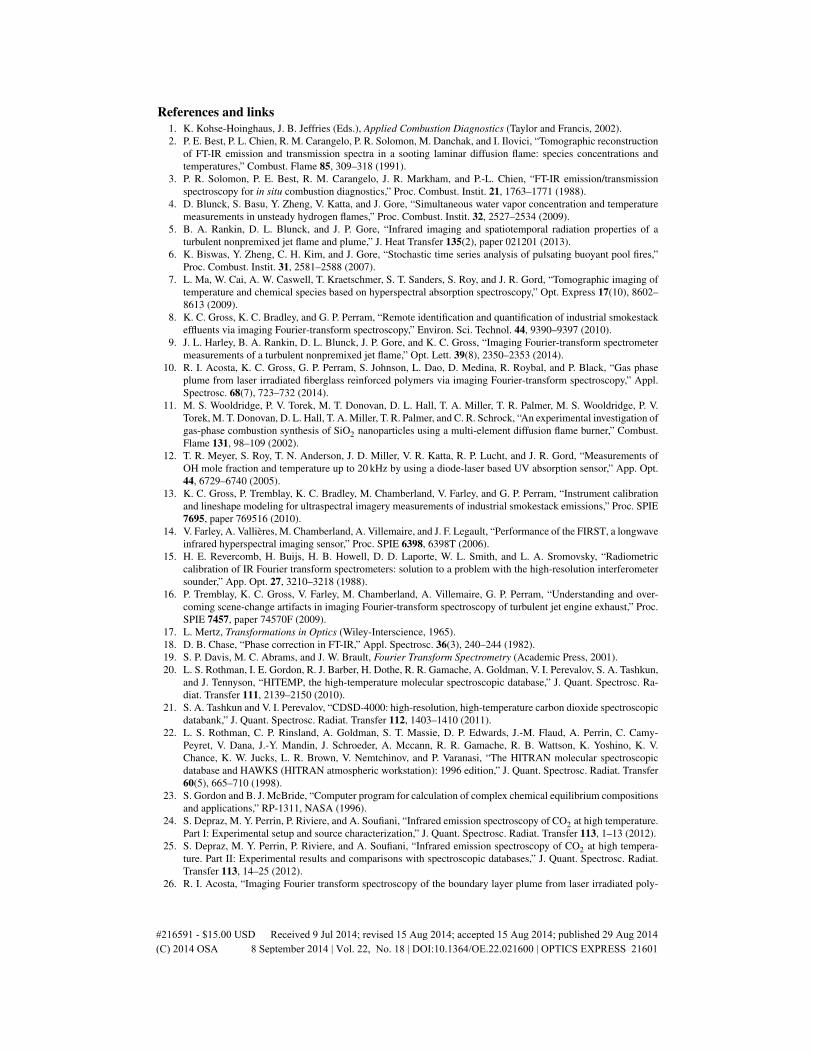
Fig. 2. Representative single-pixel gain curve magnitude computed from standard calibra-tion method (grey) compared with the gain curve magnitude obtained after atmosphericcorrection and spline smoothing (black). Residual difference between standard gain curveand the product of the smooth gain curve with atmospheric transmittance function is pro-vided, offset by −1 a.u./r.u.. Atmospheric absorption features are annotated. Here, a.u. rep-resents arbitrary units and r.u. represents radiometric units.

decreases as 1/ν̃ across the detector bandpass. These effects reasonably limit the achievableSNR of the gain term at higher wavenumbers. Since the calibrated scene radiance is obtainedvia division by Gi(ν̃), a low-SNR gain can introduce errors in Li(ν̃) that are non-normallydistributed, complicating quantitative interpretation of flame spectra.

The InSb quantum efficiency, optics transmittances, and other factors affecting system re-sponse are such that the gain magnitude, |Gi(ν̃)|, exhibits a smooth, slow variation with ν̃ . Apossible exception to this is the effect that the atmospheric transmittance profile would have on|Gi(ν̃)|, if it is not accounted for when modeling the at-sensor radiance from a distant black-body source. Our calibration methodology accounts for atmospheric absorption, and leveragesthe expectation of smoothness of the resulting gain term. First, Mertz phase correction [17, 18]is performed when converting calibration (and flame) interferograms to raw spectra. Then aleast-squares smoothing spline is applied to each pixel’s gain magnitude and the gain phase isset to zero. (Phase correction ensured the gain phase was zero-mean noise.) It was determinedvia graphical inspection that fifteen spline points adequately captured the variation in |Gi(ν̃)|without fitting to the noise. The imaginary component of the calibrated flame radiance is notdiscarded as it can be used to assess calibration quality and estimate SNR.

Single-pixel gain curves obtained via the standard calibration method and our modified ap-proach are compared in Fig. 2. The gain determined from the standard calibration withoutatmospheric compensation is shown in grey. Overlaid with this curve is the modified gain ob-tained using atmospheric compensation and a spline fit. The residual difference between thestandard gain and the smooth gain, multiplied by the atmospheric transmittance profile, is alsoshown. The largely unstructured residuals are dominated by noise, indicating the effectivenessof the atmospheric compensation and spline smoothing.

3.3. Spectral radiation model for determining scalar values

A simple model describing the apparent line-of-sight flame radiance was used to estimate tem-perature and relative species concentrations from the measured spectra. The spectral radianceLi(ν̃) from a non-scattering source in local thermodynamic equilibrium (LTE) can be approxi-


mated byLi(ν̃) = τ(ν̃)ε(ν̃ ,T,~ξ )B(ν̃ ,T )∗ ILS(ν̃) (4)

where ε(ν̃ ,T,~ξ ) is the gas emissivity, which is a function of gas mole fractions~ξ , and B(ν̃ ,T ) isPlanck’s blackbody radiance distribution at temperature T . Here, τ(ν̃) represents the transmit-tance of the atmosphere between the flame and instrument. Measured meteorological conditionswere used to estimate τ(ν̃). ILS(ν̃) represents the instrument line shape of a Fourier-transformspectrometer with which the “monochromatic” flame spectrum is convolved. No apodizationof the interferograms was performed, thus ILS(ν̃) = 2πxmsinc(2πxmν̃) [13, 19]. In a non-scattering medium, the spectral emissivity is related to the scalar values via

ε(ν̃ ,T,~ξ ) = 1− exp

(−lN ∑

iξiσi(ν̃ ,T )

)= 1− exp

(− l

lMFP

)(5)

where the number density N = P/(kBT ), l is the path length through the flame, ξi is the ith

species mole fraction, and σi(ν̃ ,T ) is its corresponding absorption cross-section. The product~q = ~ξ l is denoted the fractional column density. The reciprocal of the number density andsum over mole-fraction weighted cross-sections defines the photon mean-free-path, lMFP, inthe model flame.

The phenomenological absorption cross-section σi for the ith species represents a sum overdiscrete spectral emission lines, each with its own line intensity, Si j, and line shape, φi j(ν̃), via:

σi(ν̃ ,T ) = ∑j

Si j(T )φi j(ν̃− ν̃ j,T ). (6)

The line shape term is dependent on the partial pressures of the various species. In this work, theVoigt profile is used and a constant pressure of P = 976hPa is assumed throughout the flame.In computing the Voigt profile, species are assumed dilute so that only broadening rates for dryair are used. Line mixing and continuum effects on the line shape were not included. Parame-ters to compute absorption cross-sections for H2O and CO were computed using the HITEMPspectroscopic database [20], and cross-sections for CO2 were computed using the CDSD-4000spectroscopic database [21]. The phenomenological cross section includes the weighting ofinternal state populations via Boltzmann statistics (assuming LTE), and the temperature de-pendence is computed (see the appendix in [22]) using the appropriate partition function dataaccompanying the HITEMP and CDSD-4000 databases. Cross-sections for each species werepre-computed at temperatures between 300 K to 3000 K every 50 K, and quadratic interpolationwas used to compute cross-sections at arbitrary temperatures.

Spectral estimates of the flame temperature and fractional column densities were determinedat each pixel by fitting Eq. (4) to the corresponding measured spectrum. This was accomplishedby minimizing the sum of squared differences between the data and model parameters, T and~q = (qH2O,qCO2

,qCO), using a Nelder-Mead direct search followed by a Levenberg-Marquardtgradient-based error minimization. Atmospheric H2O and CO2 concentrations were also modelparameters to ensure the best possible estimate of τ . In the Φ = 0.8 and Φ = 0.9 flames, asmall baseline oscillation was observed in spectral regions absent of line emission from thecombustion gases. As discussed later, this only occurred in certain flame locations and is likelythe result of insufficient temporal averaging over the flame unsteadiness. To mitigate the im-pact of the baseline oscillation on the spectral fit results, a 4th-order polynomial was added tothe model for the Φ = 0.8 and Φ = 0.9 measurements. The spectrum at each pixel contains3000 unique radiance values, ensuring the six-parameter or eleven-parameter nonlinear modelis highly over-determined.


This model makes a few notable simplifications to the actual radiative transfer problem, themost significant being the assumption of flame homogeneity along each pixel’s line-of-sight.This is a reasonable approximation near the base of the Hencken burner where—as supportedby flame images presented in the next section—the mixing layer is a small fraction of the totalline-of-sight. This assumption is also made in the analysis of OH laser absorption measurementsof the similarly configured Hencken flame against which the present results will be compared[12]. The width of the mixing layer steadily increases with height above the flame, and the ho-mogeneity approximation above ~20 mm breaks down. As the mixing layer grows, temperatureand density gradients become non-negligible and will systematically bias the fit parametersdue to the variation in T and ξi along the line-of-sight. Given these limitations, this modelcan only be used to estimate core flame temperature and concentrations near the base of theburner and along lines-of-sight that are not dominated by the mixing layer, i.e., u < 20mm and|v| < 10mm. Here u and v represent the flame coordinate system, and are defined in Fig. 3.A multi-layer deconvolution approach can be developed for flames or regions where mixing issignificant, as discussed previously. Within this region, absolute concentrations are determinedvia ξi = qi/l where l = 25.4mm/cos(θ(u)) and θ(u) = tan−1 ((u0−u)/d) is a small angle whichaccounts for the line-of-sight through the flame for rays a distance y0−y from the optical centerof the camera. Elsewhere in the flame, the biased estimates, due to mixing, of T and~q are to beinterpreted as path-averaged quantities. Note that they are not true path-averaged quantities dueto the nonlinear dependence T and ξi have on measured radiance. A multilayer deconvolutionmethod is being developed to estimate 3-D distributions of temperature and concentrations.

Other model simplifications include neglecting the transport of background radiation throughthe plume and atmospheric path radiance generated between the flame and sensor. However,these quantities are negligible compared to the flame radiance. The impact of ignoring colli-sional self-broadening in the Voigt profile has not been assessed, however its impact is expectedto be small as typical line widths are narrower than the width of ILS(ν̃).

4. Results

4.1. Data overview

Figure 3 compares the broadband imagery captured by the IFTS in a single interferometricmeasurement at each equivalence ratio. The imagery was obtained by applying a low-pass filteralong the OPD dimension with a cut-off frequency below fb.g.. The left half of each image cor-responds to the time-averaged intensity in raw camera counts. Near the base of each burner, theintensity rapidly increases with height, peaking at about 10 mm, and then decaying more grad-ually with increasing distance from the burner. The most fuel lean trial with Φ = 0.8 exhibitsthe swiftest decay in intensity with height and the fuel rich trial with Φ = 1.1 shows the slowestintensity decay with height. Traversing each flame axially, the transition from flame emissionsto background occurs near v =±13mm near the base of the burner. This mixing layer remainssmall up to about u = 10mm. Due to the symmetry of the burner, it follows that the mixinglayer represents a small contribution to the measured line-of-sight radiance near the burner.The mixing layer increases in size with additional height above the burner due to entrainmentof the N2 co-flow.

The right half of each image shows the intensity coefficient of variation (CoV), which is thestandard deviation of intensity normalized by the mean intensity. Near the base of the burner,each flame is steady, yielding intensity values on the order of 25,000 to 30,000 counts withminimal variations (CoV < 2%). Around 20 mm above the burner, buoyancy effects produceunsteady flow, causing intensity variations which increase with height and are more than 15% ofthe mean intensity by 40 mm. Unsteady intensity fluctuations were largest for the Φ = 0.9 trialwith CoV values exceeding 22% in the mixing layer near 60 mm above the burner. Interestingly,


Fig. 3. Split imagery of the symmetric flame for each of the four Φ values tested. Meancamera intensity values are on the left and coefficient of variation (CoV) values are on theright. The top and bottom of the color bar correspond to the mean intensity in 1,000’s ofcounts and CoV values, respectively.

13579111315 P71

0

500

2080 2100 2120 2140

Fig. 4. Three center-flame spectra corresponding to heights 10 mm, 60 mm and 100 mmabove the base of the Φ= 1.1 flame. The inset plots presents a detailed view of the P-branchcorresponding to the fundamental 1→ 0 emission from CO. Odd numbered rotational levelsare marked.

CoV values between 40mm≤ u≤ 90mm and v = 0 were substantially larger for the fuel lean-flames compared with the fuel-rich flames.

Center-flame spectra at 10 mm, 60 mm and 100 mm above the burner are presented in Fig. 4.The largest emission feature near 2250cm−1 is from the asymmetric stretching mode of CO2,as well as combination bands at nearly resonant frequencies. Careful inspection of the regionbetween 2000 cm−1 to 2150 cm−1 reveals the P-branch of CO (see inset plot). The R-branchoverlaps with the strong CO2 emission and becomes difficult to discern. The line emissionbetween 3000 cm−1 to 4200 cm−1 is primarily due to H2O rotational fine structure associatedwith transitions between several vibrational states. Also within this region is weaker broadbandemission from CO2, and very weak spectral emission from OH. The spectral radiance decreases


DataModel

Residuals Noise

= 1.1

0

0.2

0.4

0

500

1000

1500

2000 2500 3000 3500 4000

100

200

300

2040 2050 2060 2070 2080 2090 2100

0

200

400

005305430043

Fig. 5. Top: Ethylene Φ = 1.1 center-flame spectrum 10 mm above burner (· black) is com-pared with a model fit (– gray). Fit residuals, offset by −150µW/(cm2 sr cm−1), and in-strument noise level, offset by −350µW/(cm2 sr cm−1), are provided. Bottom: Ratio of theflame path length, l, to the calculated mean free path of a photon, lMFP, under the conditionsestimated by the model fit.

with height due to cooling brought on by mixing with the N2 co-flow and surrounding air. Theentrainment of air enables oxidation of CO to occur with increasing distance from the burner,and by 100 mm CO emission lines are substantially diminished.

4.2. 2-D spectral estimates of scalar values

4.2.1. Single pixel results

Fitting Eq. (4) enables simultaneous retrieval of T and mole fractions ξH2O, ξCO2and ξCO.

In the top panel of Fig. 5, the emission spectrum between 1975 cm−1 to 4225 cm−1 is shownfor a single pixel at location (u,v) = (10mm,0mm) for the Φ = 1.1 trial. Also provided isthe model prediction corresponding to the best-fit parameters of T = (2318±19)K, ξH2O =(12.5±1.7)%, ξCO2

= (10.1±1.0)% and ξCO = (3.8±0.3)%. The measured temperaturecompares favorably with recent laser diagnostics results [12], (2348±115)K, as well as withNASA CEA [23] equilibrium flame temperature of 2389 K. H2O, CO2 and CO mole fractionsare in good agreement with the CEA equilibrium values of 12.8%, 9.9% and 4.1% respectively.We are not aware of other experimental determinations of these same species mole fractions fora similarly configured Hencken burner to compare against.

Reported fit parameter errors are the 95% CIs due to measurement noise and the propagationof calibration uncertainties. They do not account for systematic errors in the model. Details onthe computation of parameter uncertainties is postponed until Sec. 4.3. The difference betweenthe data and model are also presented in Fig. 5, denoted Residuals, and compared with theimaginary part of the spectrum, denoted Noise. The fit residuals are mostly unstructured with aroot-mean-square (RMS) value of 10.1 µW/(cm2 sr cm−1). The RMS value of the fit residualsis only 1.5 times larger than the RMS value of instrument noise, indicating that the model


describes the flame spectrum well overall. However, some systematic errors are present. Thisis most evident from the observed structure in the residuals between 2150 cm−1 to 2400 cm−1.Within this range, the fit residual RMS value is 5.9 times larger than the instrument noise RMSvalue. However, the noise in this region is small, and the RMS fit residual in this band is only3.5% of the RMS signal. The quality of this single pixel spectral fit is representative of the fitquality across the hyperspectral image.

Mixing layer effects may contribute to the systematic fitting errors observed between2150 cm−1 to 2400 cm−1. The bottom panel of Fig. 5 shows the ratio of the flame path length,l, and the calculated mean free path of a photon, lMFP (Eq. (5)), under the conditions estimatedby the model fit. This ratio is less than 3% across most of the spectrum, but approaches 40%within the strong CO2 asymmetric-stretch emission band. This suggests that while the plumeis optically thin across most of the spectrum, some optical trapping occurs within this CO2band. It follows that emission from the mixing layer will have a larger effect within this bandin comparison with the optically thin spectral regions. This interpretation is consistent with theobservation that fit residual magnitudes relative to the signal increase with height (i.e. mixinglayer width). While the homogeneous assumption is adequate across most of the spectrum andyields spectral retrievals in good agreement with experimental and theoretical predictions, thehigh fidelity measurements may contain information about small mixing layer effects.

A second contributing factor for systematic fit errors may be associated with limitations of thespectroscopic databases used in this work. Recent measurements [24, 25] of high-temperature(2000 K to 5000 K) CO2 produced via microwave discharge suggests that systematic errorsin the spectral radiance between 2100 cm−1 to 2450 cm−1 can be up to 10–30%. Similarly,in a recent study involving laser irradiation of graphite targets [26], an empirical emissivitycorrection factor was needed to adequately reproduce the observed spectral emissions from thehot, CO2-rich plume above the target within this same spectral region. However, in both of theserecent experiments, CO2 temperatures were much larger than the flame temperatures observedin this work and, in some cases, exceeded the useful temperature range of the CDSD-4000database. Moreover, the radiative transfer models required to accurately describe the data wereconsiderably more complicated than what is needed to model the Hencken burner flame. Thus,while limitations of the spectroscopic databases cannot be ruled out, their effect on the scalarestimates is likely small given both the good fit quality and the excellent agreement betweenspectrally-retrieved scalar values with Meyer’s results and CEA thermodynamic calculations.

Finally, the point-spread function of the instrument causes subtle mixing of spectral emis-sions from nearby pixels, and our instrument model does not yet account for these effects.As our future efforts will focus on three-dimensional scalar field reconstruction, these smalleffects will need to be properly modeled. Given the possible systematic errors due to instru-mentation, model simplifications, and limitations of high-temperature spectroscopy databases,actual scalar value uncertainties may exceed those presented here by an additional factor oftwo. Despite this important caveat, the small fit uncertainties exemplify the benefit of a highly-resolved emission spectrum across a wide band pass for temperature estimation. 3000 uniquedata points between 1975cm−1 ≤ ν̃ ≤ 4225cm−1 sample myriad H2O, CO2 and CO emissionlines, each representing a transition between pairs of internal energy levels. When local ther-modynamic equilibrium prevails, the population of each internal energy level is governed bythe same temperature via the Boltzmann distribution.

4.2.2. Radial and axial fit results

Spectrally-estimated scalars were uniform across the flame near the base of the burner. Fig-ure 6 shows the results for the Φ = 1.1 trial at u = 10mm. The mean temperature obtainedfor all pixels within 5mm of flame center was T = 2317K with a standard deviation of 2 K.


0

5

10

15

0

2

4

15 10 5 0 5 10 150

5

10

15

15 10 5 0 5 10 15

NASA CEAOH-LA

IFTS1800

2000

2200

2400

Burner width Burner width

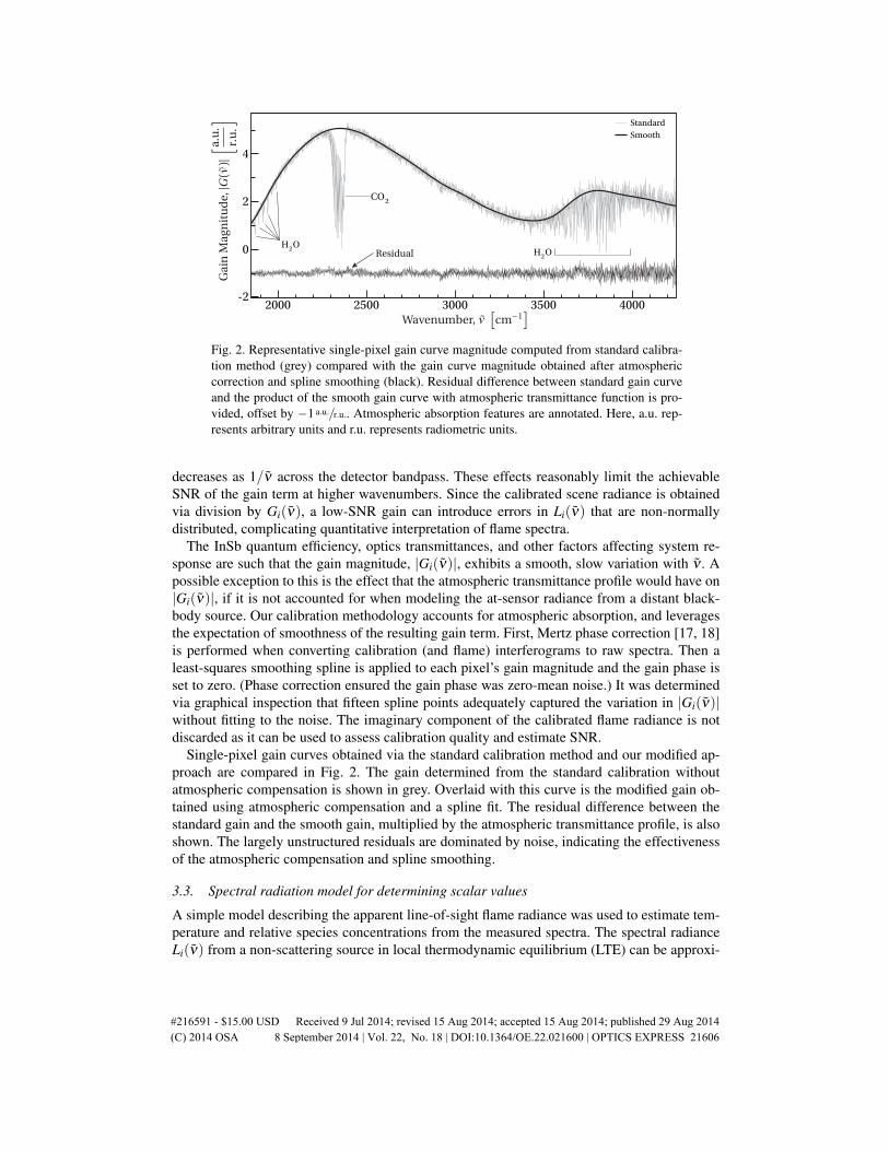
Fig. 6. Spectrally-retrieved scalar values of ethylene flame 10 mm above the burner forthe Φ = 1.1 condition. Error bars indicate the 95% confidence interval and only everyother bar is shown for clarity. For comparison, the temperature value obtained by OH-laserabsorption measurements (•) and NASA CEA values (— ,— ,— ) are provided.

EquilibriumAbsorptionIFTS

2000

2100

2200

2300

2400

2500

0.8 0.9 1.0 1.1 1.2 1.3

Fig. 7. Variation of spectrally-retrieved average temperature with equivalence ratio in ethy-lene flame at a height of 10 mm above the burner. Comparison values of temperature meas-ured with OH-laser absorption and chemical equilibrium are from Meyer et al. [12].

Note that the pixel-to-pixel temperature variance is approximately ten times smaller than the fiterrors associated with the individual spectral estimates (nominally 20 K). For comparison, thecorresponding laser-based temperature measurement is also provided. The transition to lines-of-sight dominated by radiance from the mixing layer occurs around ±10mm from the centerof the burner; beyond this, the retrieved temperature rapidly decays with distance. While theH2O and CO2 mole fraction profiles are qualitatively similar in shape to that of temperature, theCO profile is less flat across the center of the flame. Mean values within 5mm of flame centerfor H2O, CO2, and CO were 12.5% and 10.1%, and 3.8%, respectively. Pixel-to-pixel standarddeviations (0.1%, 0.08%, and 0.08%, respectively) were much smaller than measurement un-certainties. The reduction in both temperature and mole fraction in the mixing layer result inSNRs too low to support spectral retrievals beyond v =±15mm.

Temperatures estimated at u = 10mm for each equivalence ratio are compared with the laserabsorption measurements [12] and equilibrium calculations in Fig. 7. The results are in verygood agreement. IFTS temperature estimates are well within the error bars of the laser-basedmeasurements, and don’t differ by more than 30K. (The error bars provided by Meyer et al. are


5 mm 10 mm 20 mm 40 mm

1600

1800

2000

2200

15 10 5 0 5 10 15

OH-LA

IFTS

2000

2100

2200

2300

2400

0 10 20 30 40

Burner Width

Fig. 8. Left panel: Spectrally-retrieved temperature of ethylene flame at heights of 5 mm,10 mm, 20 mm and 40 mm above the burner for the Φ = 0.9 condition. Error bars are notshown for clarity but have nominal half-widths of approximately 20 K. Right panel: Com-parison of the spectrally-estimated temperatures (IFTS) with laser absorption measure-ments (OH-LA) at various heights along the centerline of the Φ = 0.9 flame. Error barsare omitted at every other point for clarity.

not clearly defined and may not represent 95% CIs.) However, with the exception of the Φ= 1.3case, spectrally-estimated temperatures are lower than those reported by Meyer.

The left panel of Fig. 8 presents the spectrally-estimated temperature profiles for all pixelswith a sufficient signal-to-noise ratio at heights of 5 mm, 10 mm, 20 mm and 40 mm abovethe burner for the Φ = 0.9 flame. Error bars are not displayed to improve visualization, buterrors are nominally ±1%. The temperature profiles at heights of 5 mm and 10 mm are flatand rapidly decay within the thin mixing layer near v =±12.5mm. This nearly top-hat profileis consistent with the approximation of the flame as a single, homogeneous layer. However, atu = 20mm, the mixing layer has widened slightly, and by u = 40mm, the flame core only spans|v| ≤ 4mm. The right panel of Fig. 8 compares spectrally-retrieved temperature of the Φ = 0.9flame traversing vertically through the centerline (v = 0) with Meyer’s OH absorption results[12]. Temperature increases rapidly above the base of the flame and peaks near 10 mm. Thespectrally-estimated results are in good agreement with the laser measurements at each heightinvestigated in Meyer’s work.

The variation in scalar values with distance from the burner is presented for all equivalenceratios in Fig. 9. The results should be interpreted as path-averaged scalar values to recognize thesignificance of temperature and concentration gradients along the line-of-sight which becomemore prominent with increasing height. The cooler, outer edge of the flame contributes less tothe path-integrated signal, so path-averaged temperatures will be lower than the center flametemperature. Additionally, the increasing size of the mixing layer makes it difficult to estimateabsolute concentrations, so column densities are reported instead. The current two-dimensionalpath-averaged results are valuable for qualitative understanding of the flame. However, quanti-tative interpretation at heights u > 10mm is not recommended since the impact of the mixinglayer—which widens with height—is not accounted for. Retrieving three-dimensional scalarfields using a deconvolution technique is the ultimate goal of this effort.

Of particular interest is the variation in scalar values with equivalence ratio. All scalar valuesimmediately increase with u. At each equivalence ratio, temperature, qH2O(u), and qCO2

(u)rapidly increase and peak between 9mm≤ u≤ 12mm. The initial behavior of qCO(u) is similar,but it reaches a maximum between 2mm ≤ u ≤ 4mm. After reaching their peak values, thescalar quantities exhibit a gradual decay with u in a manner that is highly dependent on Φ.In the fuel lean flames (Φ = 0.8,0.9), the oxygen rich environment enables quick conversion


= 1.1

= 1.3

= 0.9

= 0.8

= 0.8

= 0.9

= 1.1

= 1.3

10

15

20

25

1600

1800

2000

2200

2400

0 20 40 60 80 100 120

= 0.8

= 0.9 = 1.1

= 1.3

5

10

15

20

25

30

350 20 40 60 80 100 120

= 0.8

= 0.9

= 1.1

= 1.3

0

5

10

15

0 20 40 60 80 100 120

0 20 40 60 80 100 120

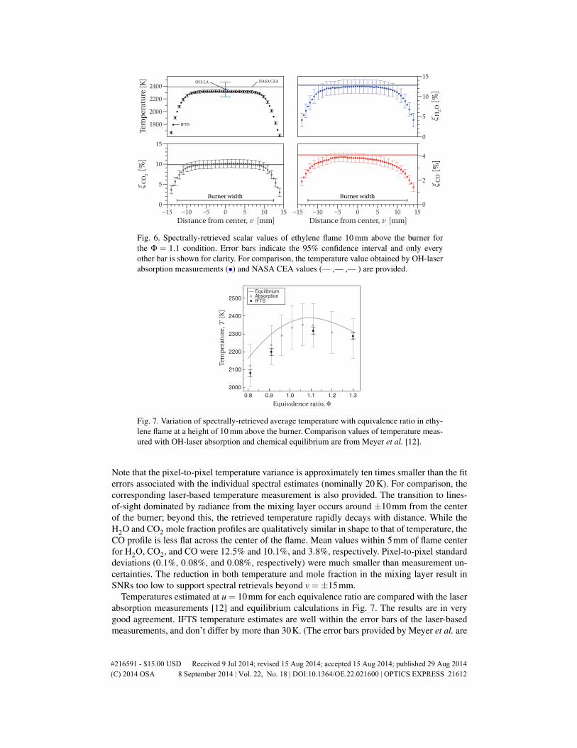
Fig. 9. Spectrally-retrieved scalar values of the C2H2/air flame, along the centerline (v= 0),for Φ = 0.8 (• red), Φ = 0.9 (• blue), Φ = 1.1 (• black), and Φ = 1.3 (• green). Error barsare omitted for clarity. Fit results obtained without the polynomial baseline correction forΦ = 0.8 (— red) and Φ = 0.9 (— blue) are annotated.

of CO to CO2, and the CO2 profiles follow an axial profile similar to H2O. In the fuel richflames (Φ = 1.1,1.3), the oxygen lean environment results in much larger CO concentrationsnear the burner and a more gradual conversion of CO to CO2. While the N2 co-flow limitsdiffusion of surrounding air into the flame, above u = 30mm, the buoyancy forces lead to flameunsteadiness, and the entrainment of atmospheric O2 is likely. (Recall the CoV map in Fig. 3.)It is reasonable that this increases the rate of CO→ CO2 conversion, as evidenced by a slightincrease in slope of the qCO2

(u) curve for Φ = 1.1 and a substantial increase in slope for Φ =1.3. The enhanced oxidation of CO at this height may be responsible for the observable changein the corresponding T (u) curve. Between 10mm≤ u≤ 30mm, the T (u) slope is −3.9 K/mmand −5.5 K/mm for Φ = 1.1 and Φ = 1.3, respectively. Between 40mm ≤ u ≤ 70mm, theslopes increase to −3.4 K/mm and −3.3 K/mm for Φ = 1.1 and Φ = 1.3, respectively.

As mentioned briefly before, spectra between 40mm ≤ u ≤ 90mm for Φ = 0.8, and to alesser extent for Φ = 0.9, exhibit a subtle, low-frequency baseline oscillation. This oscillationproduced a small bias in the T and qCO fit parameters, and prompted the pragmatic additionof the 4th-order polynomial to the model for the fuel-lean flames. This was the minimum orderneeded to visually account for the baseline oscillation; however, polynomials up to 7th-orderdid not significantly affect the fit results. The baseline oscillation is a small fraction of the totalsignal and the polynomial never represented more than 1.5% of the peak spectral radiance. Thebaseline oscillation is likely a result of insufficient averaging over the intensity fluctuations aris-ing from unsteady behavior in this flame region. It was not perceptible in the fuel-rich cases,and this is consistent with the smaller CoV values at v = 0 observed in Fig. 3. For compari-son, the fit results obtained without using the 4th-order polynomial to model the baseline areprovided in Fig. 9 for context. The difference in qCO2

(u) is imperceptible. While the baseline


2200210020001900180017001600150014001300 2300

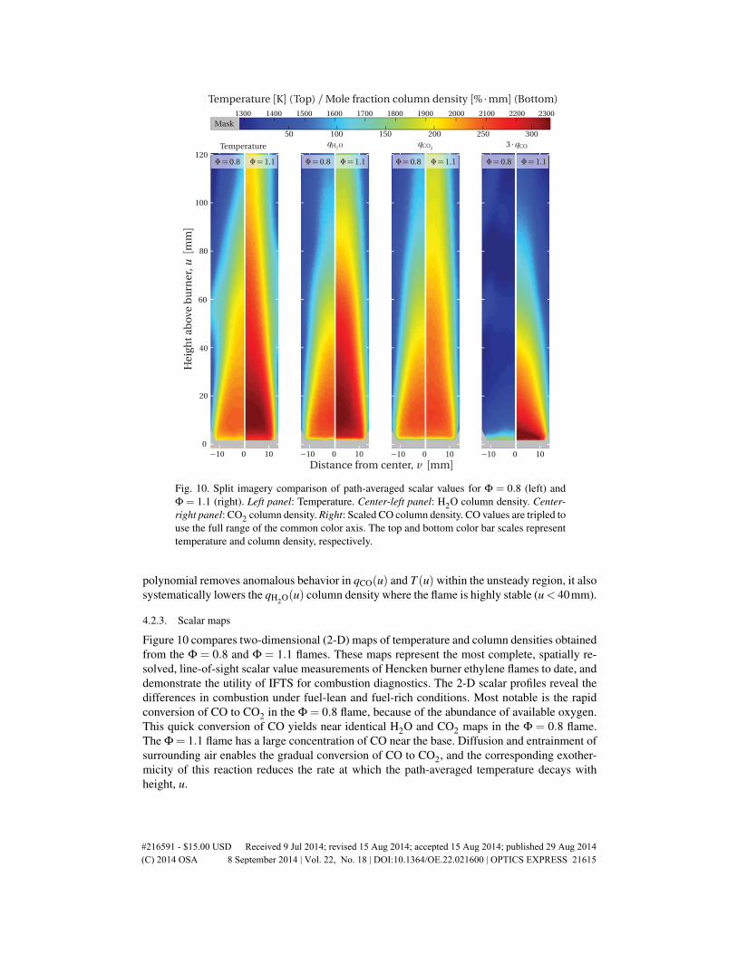
Fig. 10. Split imagery comparison of path-averaged scalar values for Φ = 0.8 (left) andΦ = 1.1 (right). Left panel: Temperature. Center-left panel: H2O column density. Center-right panel: CO2 column density. Right: Scaled CO column density. CO values are tripled touse the full range of the common color axis. The top and bottom color bar scales representtemperature and column density, respectively.

polynomial removes anomalous behavior in qCO(u) and T (u) within the unsteady region, it alsosystematically lowers the qH2O(u) column density where the flame is highly stable (u< 40mm).

4.2.3. Scalar maps

Figure 10 compares two-dimensional (2-D) maps of temperature and column densities obtainedfrom the Φ = 0.8 and Φ = 1.1 flames. These maps represent the most complete, spatially re-solved, line-of-sight scalar value measurements of Hencken burner ethylene flames to date, anddemonstrate the utility of IFTS for combustion diagnostics. The 2-D scalar profiles reveal thedifferences in combustion under fuel-lean and fuel-rich conditions. Most notable is the rapidconversion of CO to CO2 in the Φ = 0.8 flame, because of the abundance of available oxygen.This quick conversion of CO yields near identical H2O and CO2 maps in the Φ = 0.8 flame.The Φ = 1.1 flame has a large concentration of CO near the base. Diffusion and entrainment ofsurrounding air enables the gradual conversion of CO to CO2, and the corresponding exother-micity of this reaction reduces the rate at which the path-averaged temperature decays withheight, u.


NASA CEA

95% CI Range = 0.011

0

50

100

150

0.090 0.095 0.100 0.105 0.110 0.115

NASA CEA

95% CI Range = 0.018

0.11 0.12 0.13 0.14 0.15

NASA CEA

Laser Absorption

95% CI Range = 19.1 K

0

0.02

0.04

0.06

0.08

2300 23500

20

40

60

80

NASA CEA

95% CI Range = 0.0036

0.036 0.038 0.040 0.0420

100

200

300

400

Fig. 11. Uncertainty distributions estimated from a 2,000 iteration Monte Carlo analysisto propagate calibration source uncertainties to the spectrally-retrieved scalar values. Theshaded areas are centered at the mean value and correspond to the 95% confidence interval.Previous experimental and equilibrium results are provided for context.

4.3. Uncertainty estimation

An important source of systematic error in the spectrum, and consequently the estimation inscalar values, arises from imperfections in the calibration blackbody sources. High-temperature,wide-area blackbodies are necessary for calibrating flame measurements, but these are not asaccurate as smaller blackbodies designed for calibrating lower temperature scenes. To assess theimpact of absolute temperature and spectral emissivity uncertainty on the spectrally-retrievedscalar values, a Monte Carlo error analysis was performed. The manufacturer-specified 95%CIs for set-point temperatures and emissivities defined normal distributions from which ran-dom values were drawn. 2,000 iterations were performed, each time calibrating using black-body temperatures and emissivities drawn from their respective uncertainty distributions. Witheach iteration, the spectral fits were performed leading to a distribution of scalar values whichcapture the uncertainty due to calibration. In general, these systematic calibration errors (δcal)were larger than the statistical uncertainty determined from the non-linear regression (δnlr). Inthis work, scalar value uncertainties represent the root quadrature sum of these two sources,

i.e. δtotal =√

δ 2nlr +δ 2

cal.The uncertainty distributions of T , ξH2O, ξCO2

and ξCO obtained from the Monte Carlo erroranalysis of the Φ = 1.1 flame spectrum at (u,v) = (10mm,0mm) are presented in Fig. 11. Con-tinuous probability distribution functions were estimated via kernel density estimation using theEpanechnikov kernel. The 95% CI for temperature spans 2307 K to 2326 K, which is more than5 times larger than the regression uncertainty of 3.5 K. Adding in quadrature both the statis-tical fit error and the calibration systematic error yields a spectrally-estimated temperature ofT = (2318±19)K. Calibration errors had a much larger impact on the uncertainty of concen-


trations. For example, the H2O mole fraction 95% CI (11.85 % to 13.64 %) is 15 times largerthan the statistical fit uncertainty (0.12 %). Quadrature addition yields ξH2O = (12.6±0.8)%.The impact on the other flame species was similar and is reported in Fig. 11. Uncertainties ofa few percent in blackbody temperature and emissivity affect the absolute radiometric accu-racy much more than the relative spectral shape. Since the spectrally-retrieved temperature isstrongly influenced by the relative line heights, whereas the column densities are dominated bythe absolute line heights, the relative errors in temperature are much smaller than relative errorsin column density.

5. Conclusions

This investigation of an ethylene flame (Φ = 0.8− 1.3) sought to establish IFTS as a usefulcombustion diagnostic. Spectrally-determined temperatures at all Φ values agree with previouslaser absorption flame measurements of a similarly-configured Hencken burner. The large num-ber of ro-vibrational emission lines and band structures arising from multiple species lead tostatistical temperature uncertainties less than 50K in the homogeneous flame region. Addition-ally, the retrieved H2O, CO2 and CO mole fractions are in excellent agreement with equilibriumpredictions. The 2-D scalar fields obtained enable both the visualization and quantitative com-parison of the Φ-dependent chemistry throughout the flame.

IFTS offers several unique advantages for combustion diagnostics. First, it is portable andcan be set up and collecting calibrated spectral imagery in about an hour. Second, it enablesthe measurement of a moderate resolution spectrum (up to 0.25cm−1) across a wide band pass(1.5 µm to 5.5 µm). This represents highly constraining data which can be used to benchmarkcomputational fluid dynamics simulations. As demonstrated, the spectra are readily interpretedin terms of 2-D path-averaged temperature and column density maps. Moreover, the adaptationof existing deconvolution algorithms to the high-fidelity hyperspectral flame images may enablethe retrieval of the 3-D scalar fields. The high-speed imagery existing within the interferometricmeasurement enables visualization of flame dynamics, and this enhances interpretation of 2-Dscalar fields derived from the time-averaged spectra. Additionally, existing flow field analysescurrently performed by infrared cameras can be readily adapted to the broadband imagery cap-tured within the IFTS measurement. However, as a passive measurement, IFTS does not havethe same sensitivity to trace species that lasers enjoy, and homonuclear diatomic molecules(e.g. H2) cannot be observed. Additionally, the slow speed (0.1 Hz to 10 Hz) at which typi-cal IFTS measurements are captured requires statistically significant numbers of observations(100–1000) to properly average over temporal fluctuations in the scalar fields.


mid-ir hyperspectral imaging of laminar ﬂames for … · 1department of engineering physics, air...

Documents