Microwave Imaging of Biological Tissues: the

current status in the research area

Tommy Gunnarsson ∗

December 18, 2006

∗Department of Computer Science and Electronics, Malardalen University

Abstract

Microwave imaging is a non-ionizing method promising an ability of depth-scanning different biological bodies. The research in this area started in thelate 70s and many contributions has been achieved by different groups untilpresent, which have influenced and open up new possibilities of the technique.This document will review the historical work by the different groups to settleobjectives of the research in microwave imaging at the Department of Com-puter Science and Electronics at Malardalen University and the plan of theauthor’s Ph. D. studies. The planar 2.45 GHz microwave camera located atSupelec, France, may be a very useful platform in early studies of the three-dimensional properties of microwave imaging for breast tumor detection. Byapplying the developed Newton-Kantorovich algorithm to the planar cameraa solid state of the art platform for quantitative reconstruction of inhomoge-neous objects may be established.

Contents

1 Introduction 1

2 Developed Hardware Setups 22.1 Microwave Tomography Systems Performing in Frequency-Domain . 2

2.1.1 The Planar Microwave Camera . . . . . . . . . . . . . . . . . 22.1.2 The 64 Antenna Circular Microwave Camera . . . . . . . . . 32.1.3 The 32/32 Antenna Circular Microwave Scanner . . . . . . . 42.1.4 The Clinical Circular Prototype Scanner for Biological Imaging 52.1.5 The 434 MHz Circular Microwave Scanner . . . . . . . . . . . 92.1.6 Fully 3-D Microwave Scanners . . . . . . . . . . . . . . . . . 10

2.2 Microwave Tomography Systems Using a Time-Domain Approach . 132.2.1 The Chirp Pulse Microwave Computed Tomography, CP-MCT 132.2.2 Time-Domain Microwave Tomography . . . . . . . . . . . . . 16

2.3 Microwave Microwave Imaging Using a Radar Technique Approach . 172.3.1 The Space-Time Beamforming Radar approach . . . . . . . . 17

3 The Tomographic Algorithm Development 193.1 The Diffraction Tomography . . . . . . . . . . . . . . . . . . . . . . 193.2 Non-Linear Iterative Algorithms . . . . . . . . . . . . . . . . . . . . 23

3.2.1 The Physical Description . . . . . . . . . . . . . . . . . . . . 243.2.2 The Forward Solution . . . . . . . . . . . . . . . . . . . . . . 253.2.3 The Inverse Optimization Process . . . . . . . . . . . . . . . 263.2.4 The Development of the Non-Linear Inverse Scattering in Mi-

crowave Imaging . . . . . . . . . . . . . . . . . . . . . . . . . 28

4 The Phantom Model Development 31

5 Discussion and Future Work 33

6 Conclusions 33

1 Introduction

Microwave imaging is a non-ionizing method which promises the ability of depth-scanning different dielectric bodies for biomedical applications. This method hasbeen proved able to detect malignant tumors as the dielectric properties of thesediffer from other human tissues. The contrast in permittivity for different in-vivotissues (bone, fat, malign tumor, vascular tissue etc.) is much higher compared tothe density contrast X-Ray Computed Tomography (CT) can yield [1]. For thisreason, microwave imaging has been developed as a complementary modality tomammography[2, 3]. However, microwave imaging needs a improvements in bothhardware platforms and imaging algorithms to be considered as a reliable and quan-titative modality for biomedical application. The complexity of biomedical tissuesmakes the wave propagation complicated and demanding high sensitivity in thehardware. The scattering phenomenon in microwave imaging is highly non-linearand demands a great amount of calculation capabilities to reconstruct an imagewith reasonable quality. Impressive results in inverse scattering algorithms for two-dimensional scenarios have been obtained by [1, 4, 5, 6], resulting in tomographicimaging of bodies with complex dielectric permittivity[1, 5, 7, 68, 69]. The tomo-graphic algorithms must be further developed to improve the convergence of theinverse problem and a more stable platform must be established before the tech-nique can be considered as a useful complementary technique in the biomedicalarea.

In this document earlier research in the area of microwave imaging of biologi-cal tissues will be reviewed and summarized, from the beginning of the 80s untilpresent. First the hardware development will be discussed, followed by the algo-rithm development. In the end, the specific phantom model developing for thebreast tumor detection application is discussed. The last section points out somepossible future directions in this area.

1

2 Developed Hardware Setups

Several hardware setups have been developed during the last three decades. Thefirst successful experiments where performed by Larsen and Jacobi in the late 70s,resulting in images showing the internal structures of canine kidneys. These experi-ments where made, using two antennas and measuring the transmission coefficientsbetween them with a mechanical rotation around the object [10]. These resultsconstructed a major foundation opening up the future of microwave imaging ofbiological tissues.

2.1 Microwave Tomography Systems Performing in Frequency-Domain

2.1.1 The Planar Microwave Camera

One of the first imaging systems developed was the planar microwave camera byBolomey et al. during the 80s. This planar microwave camera includes two largehorn-antennas, one transmitter and one receiver, with a water tank in between. Thetransmitting antenna is designed to produce an approximately plane wave which isreceived in the receiving antenna, depicted in Figure 1. The object is immersed ofwater into the water tank and the scattered field due to the object is measured alonga plane behind the object. The camera using 1024 dipole antennas on a plane matrixplaced on the water tank in front of the receiving horn antenna, also named thecollector. The antenna matrix forms a syntectic retina where the antenna elementsdistributing the plane-wave passing it. The retina is not considered as a receiverwhile it disturbs the field before the receiving collector in a Modulated ScatteringTechnique(MST) fashion[11]. Using this technique one antenna element is activeat the time by a modulation of 200 kHz, the received signal in the collector givesinformation of the field properties at the antenna element position. By scanningthrough all elements of the retina quick data acquisition is archived using a relativelysimple hardware[12]. This because the retina elements is modulated by a frequencyof 200 kHz, which modulates the planar carrier wave frequency of 2.45 GHz, onlytwo high frequency channels is needed for 1024 measurements points.

Using lower frequency the multiplexer controlling the sensor matrix may besimplified. This camera was developed with the main goal to produce qualitativeimages of the temperature distribution of biological tissues to control the effectduring hyperthermia treatment [13, 14]. The camera has been further developedsince then to produce quantitative results [15] as well as qualitative results in a quasireal-time manner [16]. Ann Franchois was able to produce quantitative results ofa homogenous cylinder, with the conclusion that the calibration of the incidentfield was one of the main issues to improve the quantitative result [15]. While aquasi real-time acquisition time of the image is a useful issue in many biologicalapplications Alain Joisel have further developed the real-time functionality of the

2

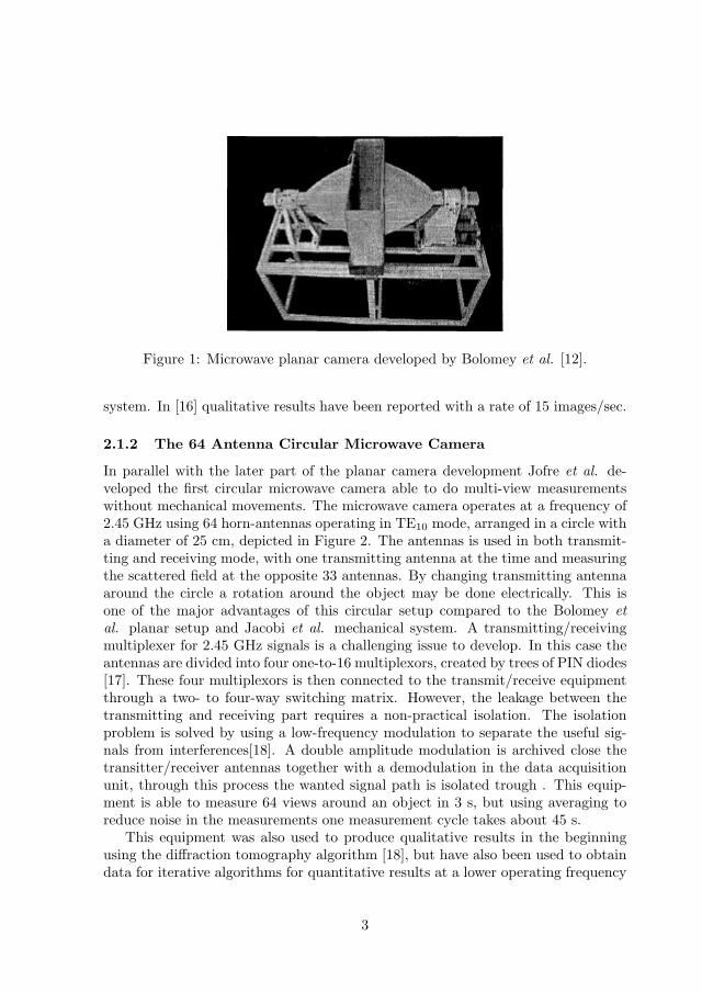
Figure 1: Microwave planar camera developed by Bolomey et al. [12].

system. In [16] qualitative results have been reported with a rate of 15 images/sec.

2.1.2 The 64 Antenna Circular Microwave Camera

In parallel with the later part of the planar camera development Jofre et al. de-veloped the first circular microwave camera able to do multi-view measurementswithout mechanical movements. The microwave camera operates at a frequency of2.45 GHz using 64 horn-antennas operating in TE10 mode, arranged in a circle witha diameter of 25 cm, depicted in Figure 2. The antennas is used in both transmit-ting and receiving mode, with one transmitting antenna at the time and measuringthe scattered field at the opposite 33 antennas. By changing transmitting antennaaround the circle a rotation around the object may be done electrically. This isone of the major advantages of this circular setup compared to the Bolomey etal. planar setup and Jacobi et al. mechanical system. A transmitting/receivingmultiplexer for 2.45 GHz signals is a challenging issue to develop. In this case theantennas are divided into four one-to-16 multiplexors, created by trees of PIN diodes[17]. These four multiplexors is then connected to the transmit/receive equipmentthrough a two- to four-way switching matrix. However, the leakage between thetransmitting and receiving part requires a non-practical isolation. The isolationproblem is solved by using a low-frequency modulation to separate the useful sig-nals from interferences[18]. A double amplitude modulation is archived close thetransitter/receiver antennas together with a demodulation in the data acquisitionunit, through this process the wanted signal path is isolated trough . This equip-ment is able to measure 64 views around an object in 3 s, but using averaging toreduce noise in the measurements one measurement cycle takes about 45 s.

This equipment was also used to produce qualitative results in the beginningusing the diffraction tomography algorithm [18], but have also been used to obtaindata for iterative algorithms for quantitative results at a lower operating frequency

3

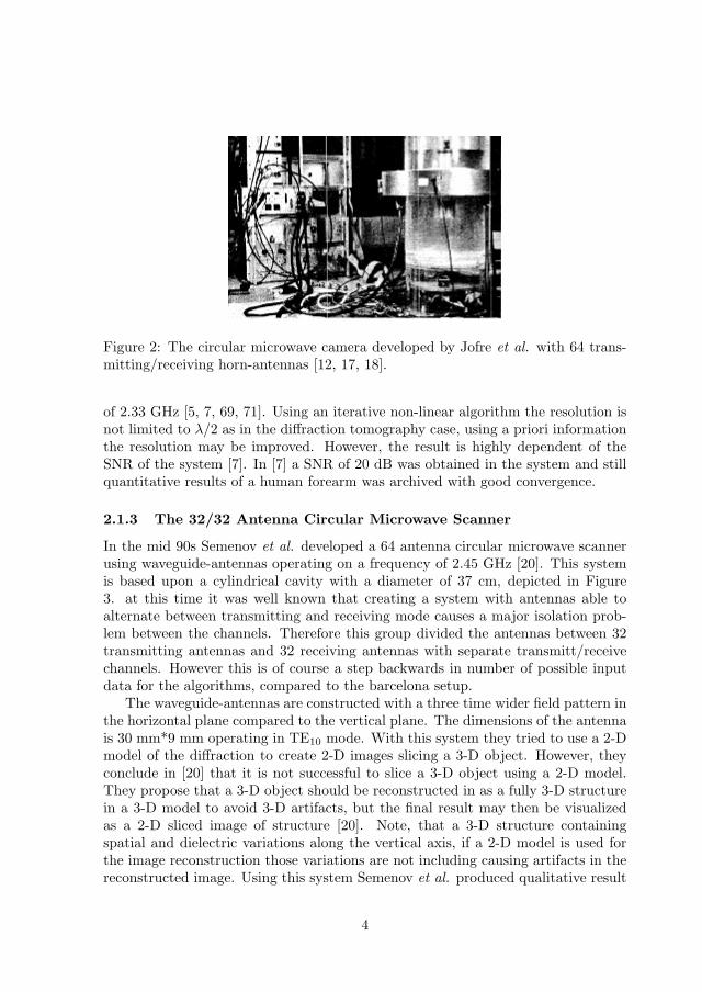
Figure 2: The circular microwave camera developed by Jofre et al. with 64 trans-mitting/receiving horn-antennas [12, 17, 18].

of 2.33 GHz [5, 7, 69, 71]. Using an iterative non-linear algorithm the resolution isnot limited to λ/2 as in the diffraction tomography case, using a priori informationthe resolution may be improved. However, the result is highly dependent of theSNR of the system [7]. In [7] a SNR of 20 dB was obtained in the system and stillquantitative results of a human forearm was archived with good convergence.

2.1.3 The 32/32 Antenna Circular Microwave Scanner

In the mid 90s Semenov et al. developed a 64 antenna circular microwave scannerusing waveguide-antennas operating on a frequency of 2.45 GHz [20]. This systemis based upon a cylindrical cavity with a diameter of 37 cm, depicted in Figure3. at this time it was well known that creating a system with antennas able toalternate between transmitting and receiving mode causes a major isolation prob-lem between the channels. Therefore this group divided the antennas between 32transmitting antennas and 32 receiving antennas with separate transmitt/receivechannels. However this is of course a step backwards in number of possible inputdata for the algorithms, compared to the barcelona setup.

The waveguide-antennas are constructed with a three time wider field pattern inthe horizontal plane compared to the vertical plane. The dimensions of the antennais 30 mm*9 mm operating in TE10 mode. With this system they tried to use a 2-Dmodel of the diffraction to create 2-D images slicing a 3-D object. However, theyconclude in [20] that it is not successful to slice a 3-D object using a 2-D model.They propose that a 3-D object should be reconstructed in as a fully 3-D structurein a 3-D model to avoid 3-D artifacts, but the final result may then be visualizedas a 2-D sliced image of structure [20]. Note, that a 3-D structure containingspatial and dielectric variations along the vertical axis, if a 2-D model is used forthe image reconstruction those variations are not including causing artifacts in thereconstructed image. Using this system Semenov et al. produced qualitative result

4

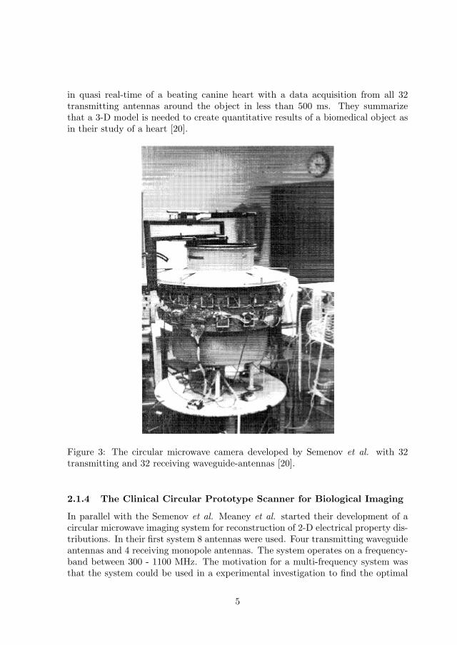
in quasi real-time of a beating canine heart with a data acquisition from all 32transmitting antennas around the object in less than 500 ms. They summarizethat a 3-D model is needed to create quantitative results of a biomedical object asin their study of a heart [20].

Figure 3: The circular microwave camera developed by Semenov et al. with 32transmitting and 32 receiving waveguide-antennas [20].

2.1.4 The Clinical Circular Prototype Scanner for Biological Imaging

In parallel with the Semenov et al. Meaney et al. started their development of acircular microwave imaging system for reconstruction of 2-D electrical property dis-tributions. In their first system 8 antennas were used. Four transmitting waveguideantennas and 4 receiving monopole antennas. The system operates on a frequency-band between 300 - 1100 MHz. The motivation for a multi-frequency system wasthat the system could be used in a experimental investigation to find the optimal

5

frequency for the imaging process as well using different frequencies to improve im-age quality and the system’s usability[21]. The antenna system operates in the TMmode, where the most of the E-field is assumed to be vertical polarized. This dataacquisition system also use amplitude modulation to increase the isolation betweenthe transmitting and receiving channel.

The long term objective of this system is also the thermal imaging during hy-perthermia treatment, like Bolomey and Jofre et al.. At this time no group hadbeen able to produce experimental quantitative results of the temperature insidelarger objects with high dielectric contrast, using the quasi real-time diffractiontomography methods. Only the differential issue of temperature differences with-out quantitative information had been obtained [17]. The approach for Meany etal. was to develop a system able produce static quantitative images of biologicaltissues. For this reason they started with an iterative inverse scattering methodwhich is more time-consuming than the earlier spectral diffraction methods [6]. Thealgorithm used was developed from the Newton-based method using a hybrid of theFinite Element and the Boundary Element method to compute the electric field ateach iteration [22, 23]. This to lower the number of unknowns and lowering thecalculation effort in the forward solver. In this step the quasi real-time function-ality is lost but what is gained is the ability to handle more complex objects withmany scatterers and high electrical property variations. In [21] the first experi-mental results are presented together with a calibration technique. In this earlystep quantitative results where produced for objects with an approximate size ofone-half wavelength.

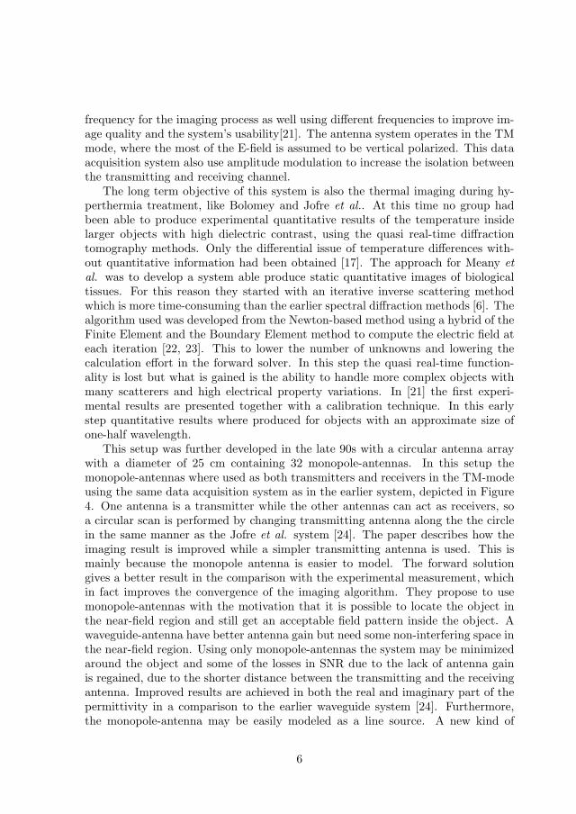
This setup was further developed in the late 90s with a circular antenna arraywith a diameter of 25 cm containing 32 monopole-antennas. In this setup themonopole-antennas where used as both transmitters and receivers in the TM-modeusing the same data acquisition system as in the earlier system, depicted in Figure4. One antenna is a transmitter while the other antennas can act as receivers, soa circular scan is performed by changing transmitting antenna along the the circlein the same manner as the Jofre et al. system [24]. The paper describes how theimaging result is improved while a simpler transmitting antenna is used. This ismainly because the monopole antenna is easier to model. The forward solutiongives a better result in the comparison with the experimental measurement, whichin fact improves the convergence of the imaging algorithm. They propose to usemonopole-antennas with the motivation that it is possible to locate the object inthe near-field region and still get an acceptable field pattern inside the object. Awaveguide-antenna have better antenna gain but need some non-interfering space inthe near-field region. Using only monopole-antennas the system may be minimizedaround the object and some of the losses in SNR due to the lack of antenna gainis regained, due to the shorter distance between the transmitting and the receivingantenna. Improved results are achieved in both the real and imaginary part of thepermittivity in a comparison to the earlier waveguide system [24]. Furthermore,the monopole-antenna may be easily modeled as a line source. A new kind of

6

calibration is also proposed which is useful for all antenna types. This calibrationtechnique improved the result even more[24].

Figure 4: The active microwave circular camera for imaging of biological materials,developed by Meaney et al. [21, 24]. (a) The tank with the 32-channel dataacquisition system in laboratory operation. (b) View of the 32 monopole-antennaarray. (c) A view of the data acquisition system mounted on a transportable chart.

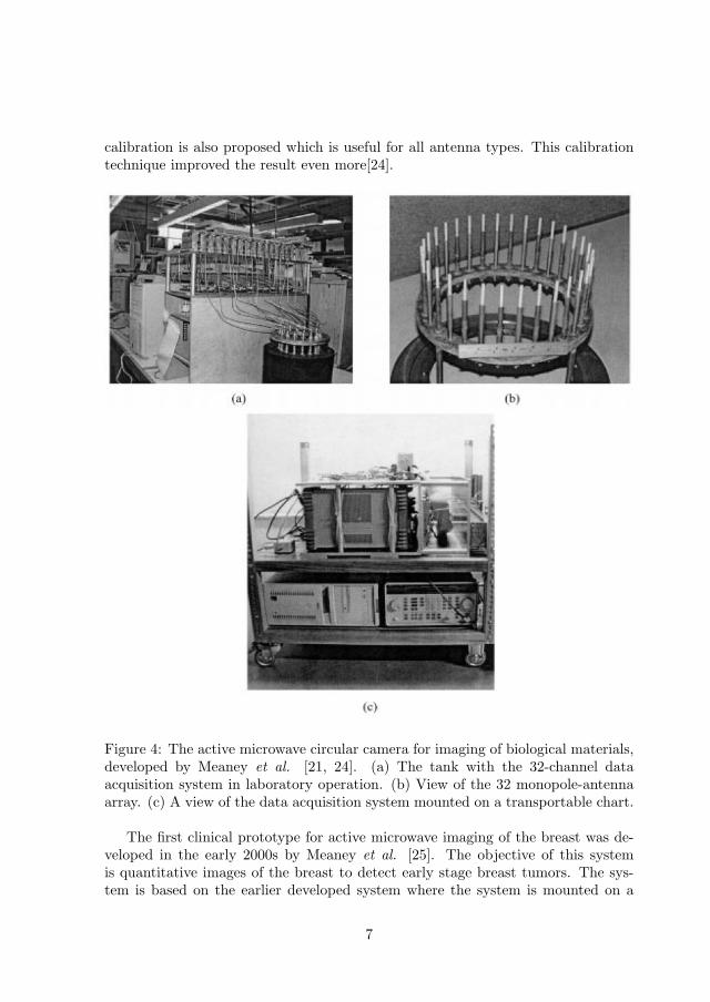
The first clinical prototype for active microwave imaging of the breast was de-veloped in the early 2000s by Meaney et al. [25]. The objective of this systemis quantitative images of the breast to detect early stage breast tumors. The sys-tem is based on the earlier developed system where the system is mounted on a

7

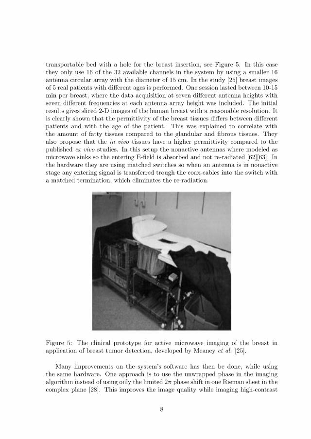
transportable bed with a hole for the breast insertion, see Figure 5. In this casethey only use 16 of the 32 available channels in the system by using a smaller 16antenna circular array with the diameter of 15 cm. In the study [25] breast imagesof 5 real patients with different ages is performed. One session lasted between 10-15min per breast, where the data acquisition at seven different antenna heights withseven different frequencies at each antenna array height was included. The initialresults gives sliced 2-D images of the human breast with a reasonable resolution. Itis clearly shown that the permittivity of the breast tissues differs between differentpatients and with the age of the patient. This was explained to correlate withthe amount of fatty tissues compared to the glandular and fibrous tissues. Theyalso propose that the in vivo tissues have a higher permittivity compared to thepublished ex vivo studies. In this setup the nonactive antennas where modeled asmicrowave sinks so the entering E-field is absorbed and not re-radiated [62][63]. Inthe hardware they are using matched switches so when an antenna is in nonactivestage any entering signal is transferred trough the coax-cables into the switch witha matched termination, which eliminates the re-radiation.

Figure 5: The clinical prototype for active microwave imaging of the breast inapplication of breast tumor detection, developed by Meaney et al. [25].

Many improvements on the system’s software has then be done, while usingthe same hardware. One approach is to use the unwrapped phase in the imagingalgorithm instead of using only the limited 2π phase shift in one Rieman sheet in thecomplex plane [28]. This improves the image quality while imaging high-contrast

8

objects without the same demands of the a priori information about object sizeand permittivity. Further, the measured log magnitude is used directly in theiralgorithms, which improves the error-rate in the measured data [3]. Using thissystem studies has been done of the 3-D artifacts caused while using a 2-D model ofa 3-D object [29], while the iterative algorithm is a fully 2-D algorithm. With theexperience from these studies a scalar 3-D/2-D algorithm has been implemented[1] to lower the 3-D artifacts in the 2-D imaging. Furthermore, improved imagequality has also been accomplished by finding the boundary of the object. If theexact boundary is found it is then possible to model the boundary properties as astep function, while the surrounding medium is known [2]. In this method, first,the object boundary must be fond to adjust the size of the FE-region to fit theobject with heterogenous medium. Outside this region the homogeneous mediumis modeled using the boundary element method. In [2] it is shown that this methodimproves the images, especially if the inhomogeneities is located near the boundaryof the object. Finally, Meaney et al. have done some effort to produce a newprototype system with a frequency band of 0.5 – 3 GHz [30]. Using this system thegroup has been able to produce images of a breast using a frequency band between600 MHz – 2.1 GHz. The bandwidth is limited by the dynamic degradation of thedata acquisition system and by the high attenuation of the lossy medium at higherfrequencies. One important point of their contribution is the fact that a simpleantenna, as a monopole antenna, can be used with success in this context with afairly wide band and simple models.

2.1.5 The 434 MHz Circular Microwave Scanner

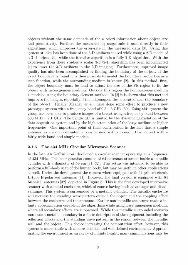
In the late 90s Geffrin et al. developed a circular scanner operating at a frequencyof 434 MHz. This configuration consists of 64 antennas attached inside a metalliccylinder with a diameter of 59 cm [31, 32]. This setup was intended to be able toperform a full-body scan of the human body, but may be useful in other applicationsas well. Under the development the camera where equipped with 64 printed circuitH-type E-polarized antennas [31]. However, the final version is equipped with 64biconical antennas [32], depicted in Figure 6. This is the first developed microwavescanner with a metal enclosure, which of course having both advantages and disad-vantages. This system is surrounded by a metallic cylinder. The metallic enclosurewill increase the standing wave pattern outside the object and the coupling affectbetween the enclosure and the antennas. Earlier non-metallic enclosures made a in-finity approximation useable in the algorithms while using lossy immersion medium,where all secondary effects are suppressed. While this metallic surrounded scenariomust use a metallic boundary in a finite description of the equipment including thereflection effects and the standing wave pattern in the region between the metallicwall and the object. This choice increasing the computation effort, however, thissystem is more stable with a more shielded and well defined environment. Approxi-mating the environment as an cavity of infinite height, many simplifications may be

9

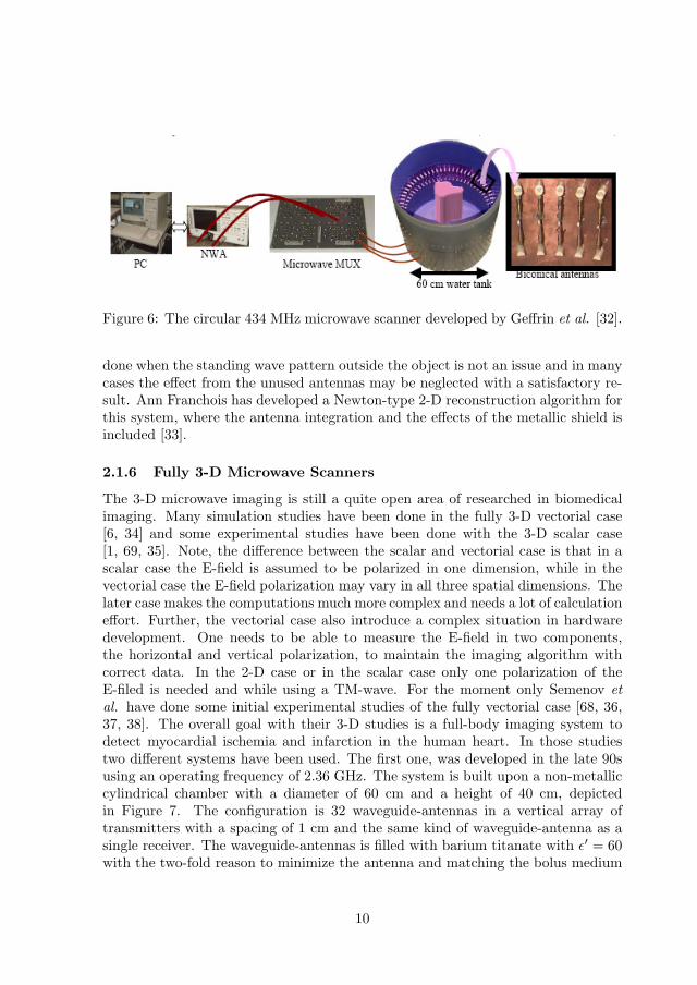
Figure 6: The circular 434 MHz microwave scanner developed by Geffrin et al. [32].

done when the standing wave pattern outside the object is not an issue and in manycases the effect from the unused antennas may be neglected with a satisfactory re-sult. Ann Franchois has developed a Newton-type 2-D reconstruction algorithm forthis system, where the antenna integration and the effects of the metallic shield isincluded [33].

2.1.6 Fully 3-D Microwave Scanners

The 3-D microwave imaging is still a quite open area of researched in biomedicalimaging. Many simulation studies have been done in the fully 3-D vectorial case[6, 34] and some experimental studies have been done with the 3-D scalar case[1, 69, 35]. Note, the difference between the scalar and vectorial case is that in ascalar case the E-field is assumed to be polarized in one dimension, while in thevectorial case the E-field polarization may vary in all three spatial dimensions. Thelater case makes the computations much more complex and needs a lot of calculationeffort. Further, the vectorial case also introduce a complex situation in hardwaredevelopment. One needs to be able to measure the E-field in two components,the horizontal and vertical polarization, to maintain the imaging algorithm withcorrect data. In the 2-D case or in the scalar case only one polarization of theE-filed is needed and while using a TM-wave. For the moment only Semenov etal. have done some initial experimental studies of the fully vectorial case [68, 36,37, 38]. The overall goal with their 3-D studies is a full-body imaging system todetect myocardial ischemia and infarction in the human heart. In those studiestwo different systems have been used. The first one, was developed in the late 90susing an operating frequency of 2.36 GHz. The system is built upon a non-metalliccylindrical chamber with a diameter of 60 cm and a height of 40 cm, depictedin Figure 7. The configuration is 32 waveguide-antennas in a vertical array oftransmitters with a spacing of 1 cm and the same kind of waveguide-antenna as asingle receiver. The waveguide-antennas is filled with barium titanate with ε′ = 60with the two-fold reason to minimize the antenna and matching the bolus medium

10

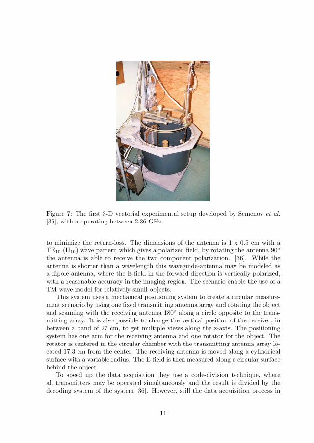
Figure 7: The first 3-D vectorial experimental setup developed by Semenov et al.[36], with a operating between 2.36 GHz.

to minimize the return-loss. The dimensions of the antenna is 1 x 0.5 cm with aTE10 (H10) wave pattern which gives a polarized field, by rotating the antenna 90o

the antenna is able to receive the two component polarization. [36]. While theantenna is shorter than a wavelength this waveguide-antenna may be modeled asa dipole-antenna, where the E-field in the forward direction is vertically polarized,with a reasonable accuracy in the imaging region. The scenario enable the use of aTM-wave model for relatively small objects.

This system uses a mechanical positioning system to create a circular measure-ment scenario by using one fixed transmitting antenna array and rotating the objectand scanning with the receiving antenna 180o along a circle opposite to the trans-mitting array. It is also possible to change the vertical position of the receiver, inbetween a band of 27 cm, to get multiple views along the z-axis. The positioningsystem has one arm for the receiving antenna and one rotator for the object. Therotator is centered in the circular chamber with the transmitting antenna array lo-cated 17.3 cm from the center. The receiving antenna is moved along a cylindricalsurface with a variable radius. The E-field is then measured along a circular surfacebehind the object.

To speed up the data acquisition they use a code-division technique, whereall transmitters may be operated simultaneously and the result is divided by thedecoding system of the system [36]. However, still the data acquisition process in

11

this system is time consuming while the receiving antenna must measure all pointson the surface at each angular position of the object, one measurement with 32directions of a 3-D object takes about 8 h to accomplish. Another problem withthe setup is that the reflection from the bottom of the chamber and the watersurface must be taken into account. This occurs while calculating the result fromthe transmitters on the outer skirt of the antenna array, while the distance is only4 cm between the array and the bottom and the water surface respectively.

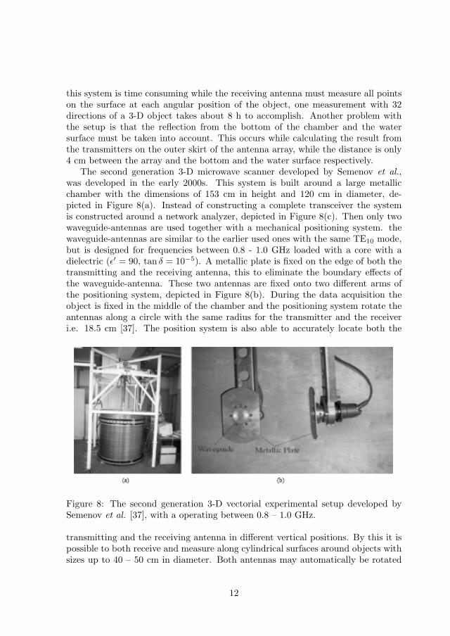
The second generation 3-D microwave scanner developed by Semenov et al.,was developed in the early 2000s. This system is built around a large metallicchamber with the dimensions of 153 cm in height and 120 cm in diameter, de-picted in Figure 8(a). Instead of constructing a complete transceiver the systemis constructed around a network analyzer, depicted in Figure 8(c). Then only twowaveguide-antennas are used together with a mechanical positioning system. thewaveguide-antennas are similar to the earlier used ones with the same TE10 mode,but is designed for frequencies between 0.8 - 1.0 GHz loaded with a core with adielectric (ε′ = 90, tan δ = 10−5). A metallic plate is fixed on the edge of both thetransmitting and the receiving antenna, this to eliminate the boundary effects ofthe waveguide-antenna. These two antennas are fixed onto two different arms ofthe positioning system, depicted in Figure 8(b). During the data acquisition theobject is fixed in the middle of the chamber and the positioning system rotate theantennas along a circle with the same radius for the transmitter and the receiveri.e. 18.5 cm [37]. The position system is also able to accurately locate both the

Figure 8: The second generation 3-D vectorial experimental setup developed bySemenov et al. [37], with a operating between 0.8 – 1.0 GHz.

transmitting and the receiving antenna in different vertical positions. By this it ispossible to both receive and measure along cylindrical surfaces around objects withsizes up to 40 – 50 cm in diameter. Both antennas may automatically be rotated

12

during the measurements to be able to measure the two-component E-field. Thesystem is able to measure attenuations as high as 120 dB with a signal-to-noiseratio of 40 dB. The usage of a large metallic chamber with a lossy medium makesit possible to ignore the boundary reflections and a free space boundary conditionmay successfully be used in the calculations.

The data acquisition may be done in three different modes. First, the simplest2-D slice where the transmitter is located at different locations along the circle andthe receiver is measuring a number of measuring points on the circle behind theobject, for each transmitter position. This is the same procedure as Jofre et al. andMeaney et al. are using but in a mechanical way. Second, for each transmittingposition along the circle, the receiving antenna is located along a 3-D cylindricalsurface behind the object and measures the 3-D distribution of the field. In thelast mode, also the transmitting antenna is located along a 3-D cylindrical surfacearound the object. At each transmitter location a 3-D surface measurement is donewith the receiver. This measurement technique is very time consuming, while thesecond method with 32 transmitting positions and 18 measuring points along thecircle in 16 different vertical positions of the receiver takes about 4.5 h [37]. Ifthen also the transmitter would be located in different vertical position the numberof data and the acquisition time may be multiplied with the number of verticalpositions, Ntv. Using this setup this group was able to improve the image qualityof fully 3-D objects, such as a full size canine [37].

2.2 Microwave Tomography Systems Using a Time-DomainApproach

A major part of the developed Microwave Tomography systems are designed to useone or several fixed frequencies in frequency domain. Another approach is, how-ever, to use a multi-frequency signal in time-domain. There is mainly two groupscontributing experimental results in this domain Miyakawa et al. and the Swedishgroup Persson et al. There solutions are completely different while Miyakawa et al.tries to linearize the problem to a straight line propagation problem using a chirppulse. Persson et al. using a non-linear algorithm working in the time-domain.

2.2.1 The Chirp Pulse Microwave Computed Tomography, CP-MCT

This modality was developed by Miyakawa et al. This group tries only to findthe straight-line projection of the traveling wave through the object, neglecting thediffraction behavior of the field. The used algorithm using the amplitude responsebehind the object similar to the already well-developed X-ray CT-algorithm. Filterout different traveling pathes using a static solution from an applied sinusoidal waveis impossible. Therefore, a chirp pulse with a specific sweep time is used, like achirp radar[40, 41]. The fastest way between the transmitter and the receiver is the

13

straight line so the system is able to pick up the straight-line chirp pulse componentfrom the received signal, in a spectral analysis in an FFT-analyzer [42].

The first system using this technique was developed by Miyakawa et al. inthe early 90s. This system used two different antennas inside a saline bath and amechanical positioning system similar to the one used in the first CT-prototype.The two antennas were moved through 128 equidistant points along two parallellines on opposite side of the object, to measure the parallel pathes through theobject. As in traditional CT this procedure was carried out at several projectionsalong a half-circle, 180o. In this system they used 50 projections with 3.6o intervals.Using a chirp pulse with a frequency between 1 – 2 GHz and a sweep time of 200ms, in each measuring point the total data acquisition takes about 100 minutes.This is far too long for a clinical application, but in the initial experiment theyreported approximately spatial resolution was 1 cm with the possibility to measuretemperature changes as low as 0.7oC [40].

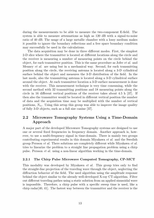
The data acquisition may be speed up by using simultaneous measurements withmodulation scattering [40], similar to the planar microwave camera of Bolomey etal.. The receiver part where exchanged to one large horn-antenna with severalmodulated PIN diode feed dipole-antennas with multiple modulation frequencies.Using multiple modulation frequencies enables parallel measurements in severaldipole positions and the system is able to accomplish faster data acquisition, theoverall principle is depicted in Figure 9. However, the conclusion was that thedata acquisition still was too long for a clinical application of in-vivo temperaturemeasurements, while it needed 4.5 minutes to complete all projections.

Figure 9: The hardware principle using modulated scattering and a chirp pulse,developed by Miyakawa et al. [40].

In the early 2000s Miyakawa et al. further developed their system with an

14

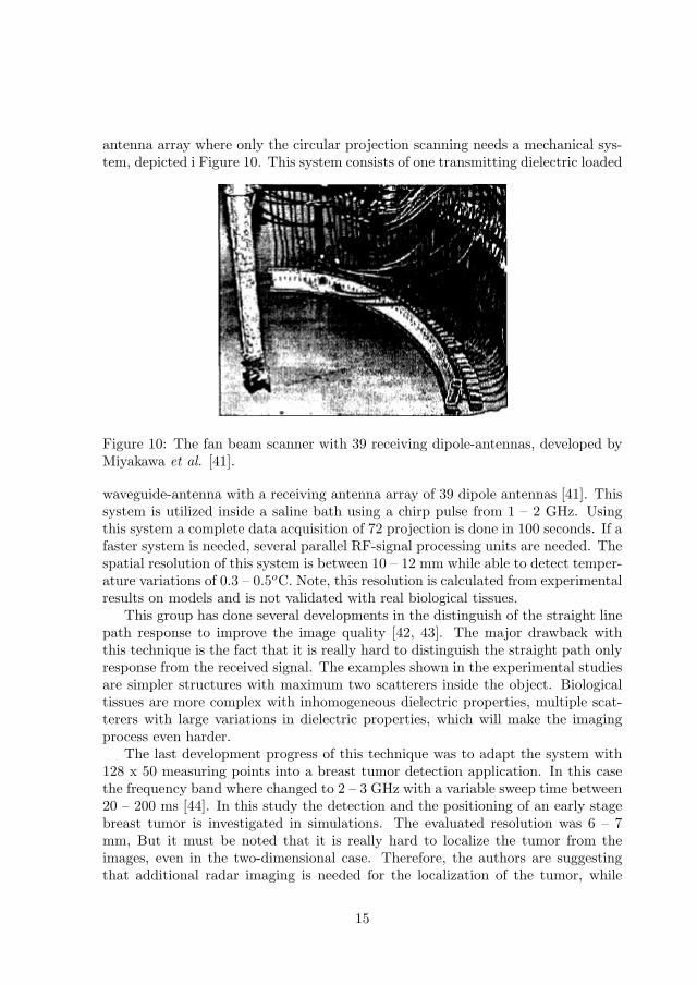
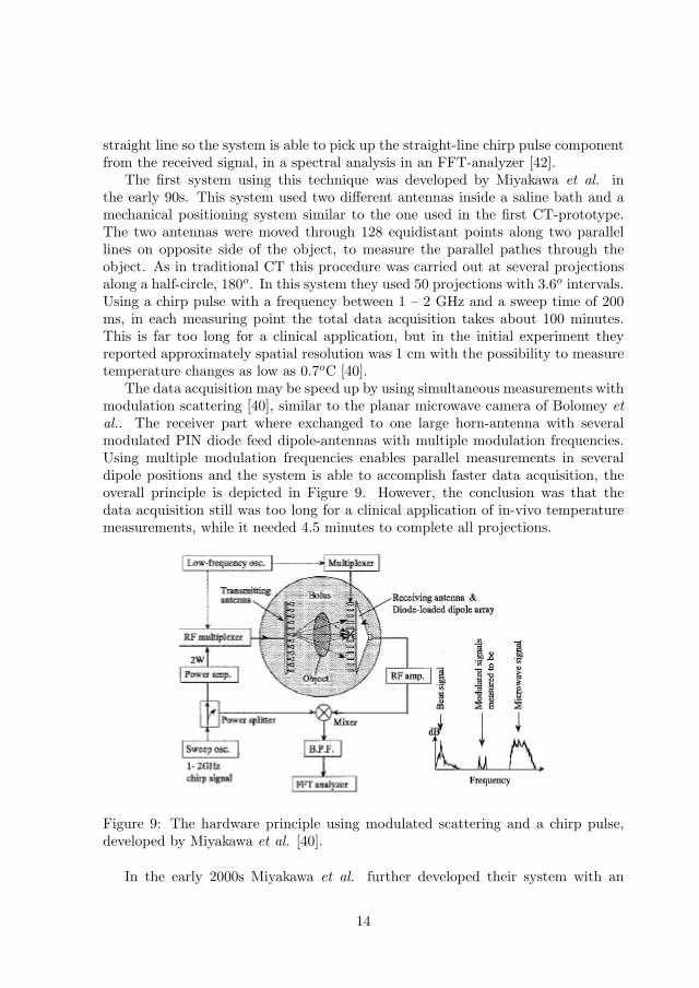
antenna array where only the circular projection scanning needs a mechanical sys-tem, depicted i Figure 10. This system consists of one transmitting dielectric loaded

Figure 10: The fan beam scanner with 39 receiving dipole-antennas, developed byMiyakawa et al. [41].

waveguide-antenna with a receiving antenna array of 39 dipole antennas [41]. Thissystem is utilized inside a saline bath using a chirp pulse from 1 – 2 GHz. Usingthis system a complete data acquisition of 72 projection is done in 100 seconds. If afaster system is needed, several parallel RF-signal processing units are needed. Thespatial resolution of this system is between 10 – 12 mm while able to detect temper-ature variations of 0.3 – 0.5oC. Note, this resolution is calculated from experimentalresults on models and is not validated with real biological tissues.

This group has done several developments in the distinguish of the straight linepath response to improve the image quality [42, 43]. The major drawback withthis technique is the fact that it is really hard to distinguish the straight path onlyresponse from the received signal. The examples shown in the experimental studiesare simpler structures with maximum two scatterers inside the object. Biologicaltissues are more complex with inhomogeneous dielectric properties, multiple scat-terers with large variations in dielectric properties, which will make the imagingprocess even harder.

The last development progress of this technique was to adapt the system with128 x 50 measuring points into a breast tumor detection application. In this casethe frequency band where changed to 2 – 3 GHz with a variable sweep time between20 – 200 ms [44]. In this study the detection and the positioning of an early stagebreast tumor is investigated in simulations. The evaluated resolution was 6 – 7mm, But it must be noted that it is really hard to localize the tumor from theimages, even in the two-dimensional case. Therefore, the authors are suggestingthat additional radar imaging is needed for the localization of the tumor, while

15

the chirp pulse microwave imaging technique may just be useful as a detectiontechnique[44]. Perhaps the chirp technique is not suitable in situations where thedielectric contrast is too large, which increases the diffraction behavior of the E-field.

2.2.2 Time-Domain Microwave Tomography

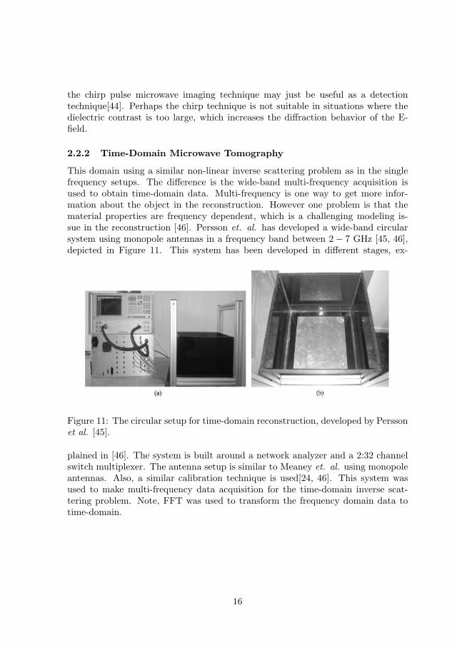
This domain using a similar non-linear inverse scattering problem as in the singlefrequency setups. The difference is the wide-band multi-frequency acquisition isused to obtain time-domain data. Multi-frequency is one way to get more infor-mation about the object in the reconstruction. However one problem is that thematerial properties are frequency dependent, which is a challenging modeling is-sue in the reconstruction [46]. Persson et. al. has developed a wide-band circularsystem using monopole antennas in a frequency band between 2− 7 GHz [45, 46],depicted in Figure 11. This system has been developed in different stages, ex-

Figure 11: The circular setup for time-domain reconstruction, developed by Perssonet al. [45].

plained in [46]. The system is built around a network analyzer and a 2:32 channelswitch multiplexer. The antenna setup is similar to Meaney et. al. using monopoleantennas. Also, a similar calibration technique is used[24, 46]. This system wasused to make multi-frequency data acquisition for the time-domain inverse scat-tering problem. Note, FFT was used to transform the frequency domain data totime-domain.

16

2.3 Microwave Microwave Imaging Using a Radar TechniqueApproach

An another microwave imaging modality is developed from the already high devel-oped microwave radar techniques. Today, a radar system may not use a rotationalantenna. By using an planar array of antenna elements with variable phase-shifts(time-shift) a electronically rotation of a beam is possible. Similar techniques maybe developed in the small-scale scenario of microwave imaging to detect inhomo-geneities inside objects. In this area Hagness et al. has developed a technique todetect early breast tumors using a a Space-Time Beamforming radar.

2.3.1 The Space-Time Beamforming Radar approach

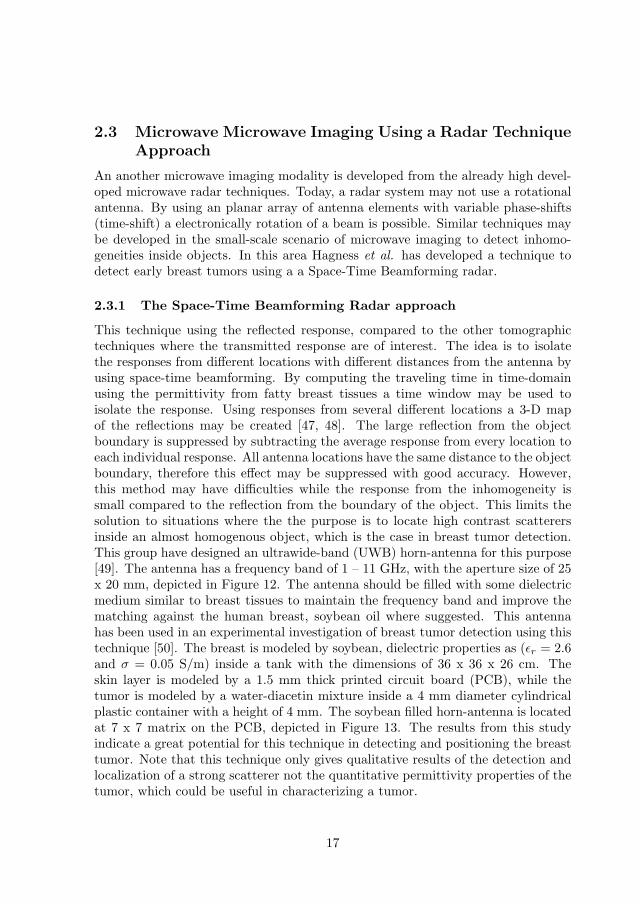
This technique using the reflected response, compared to the other tomographictechniques where the transmitted response are of interest. The idea is to isolatethe responses from different locations with different distances from the antenna byusing space-time beamforming. By computing the traveling time in time-domainusing the permittivity from fatty breast tissues a time window may be used toisolate the response. Using responses from several different locations a 3-D mapof the reflections may be created [47, 48]. The large reflection from the objectboundary is suppressed by subtracting the average response from every location toeach individual response. All antenna locations have the same distance to the objectboundary, therefore this effect may be suppressed with good accuracy. However,this method may have difficulties while the response from the inhomogeneity issmall compared to the reflection from the boundary of the object. This limits thesolution to situations where the the purpose is to locate high contrast scatterersinside an almost homogenous object, which is the case in breast tumor detection.This group have designed an ultrawide-band (UWB) horn-antenna for this purpose[49]. The antenna has a frequency band of 1 – 11 GHz, with the aperture size of 25x 20 mm, depicted in Figure 12. The antenna should be filled with some dielectricmedium similar to breast tissues to maintain the frequency band and improve thematching against the human breast, soybean oil where suggested. This antennahas been used in an experimental investigation of breast tumor detection using thistechnique [50]. The breast is modeled by soybean, dielectric properties as (εr = 2.6and σ = 0.05 S/m) inside a tank with the dimensions of 36 x 36 x 26 cm. Theskin layer is modeled by a 1.5 mm thick printed circuit board (PCB), while thetumor is modeled by a water-diacetin mixture inside a 4 mm diameter cylindricalplastic container with a height of 4 mm. The soybean filled horn-antenna is locatedat 7 x 7 matrix on the PCB, depicted in Figure 13. The results from this studyindicate a great potential for this technique in detecting and positioning the breasttumor. Note that this technique only gives qualitative results of the detection andlocalization of a strong scatterer not the quantitative permittivity properties of thetumor, which could be useful in characterizing a tumor.

17

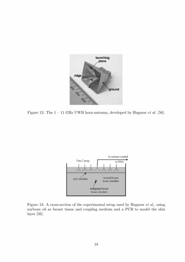
Figure 12: The 1 – 11 GHz UWB horn-antenna, developed by Hagness et al. [50].

Figure 13: A cross-section of the experimental setup used by Hagness et al., usingsoybean oil as breast tissue and coupling medium and a PCB to model the skinlayer [50].

18

3 The Tomographic Algorithm Development

In the very first experimental efforts of microwave imaging a method related toX-ray formalization based on a linear path between the transmitting and receivingantenna were used [53]. However, the physical properties of microwaves makes theimaging process using microwaves more complicated compared to X-ray ComputedTomography (CT). An X-ray travels through media with a ray pattern, while thewavelength is small compared to the object size. A microwave have a wavelengthsimilar to the object size, which makes the ray description improper describingthe spread of a traveling microwave through a biomedical object. In this case thetraveling wave will be highly affected by diffraction. Therefore, the diffraction effectmust be involved in the imaging algorithm to obtain a quantitative result of theobject.

3.1 The Diffraction Tomography

In the early 80s the first microwave tomography algorithms where developed, is-suing the diffraction phenomenon. This was in parallel during the development ofultrasonic algorithms to obtain quantitative results of soft tissues. The main ideawas to make a linear approximation of the non-linear correlation between an inho-mogeneity inside the object and the received field. One approximation is to assumethe electric field inside the object to be effected by the inhomogeneous object itself,called the Born approximation. In this case the solution is quite simple and thealgorithms obtained with a quasi real-time performance. However, this approxi-mation is shown valid only for smaller objects with small changes of the refractiveindex, e.g. weakly scattering objects [52].

In Figure 14 (left) a two-dimensional case is depicted, where a vertically polar-ized plane wave is illuminating a cylindrical object with an inhomogeneous crosssection S with the permittivity εS(x, y) and the conductivity σS(x, y). The formal-ization of a scenario like this may be as follows, assuming the total field Etot to bethe sum of the incident field Einc and the scattered field Escatt according to

Etot(x, y) = Einc(x, y) + Escatt(x, y). (1)

One may also assume that the object is located in origo of the x-y plane with aplane-wave incidence along the y-axis with a wavenumber (spatial frequency) of k0.The field is measured along a line parallel with the x-axis located at y = l, in Figure14. If the surrounding medium is homogeneous the scattered field is generated bythe equivalent currents inside the object caused by the variation of the dielectricproperties. This equivalent current may be defined as

JS(x, y) = (k2S(x, y)− k2)Etot(x, y), (x, y) ∈ S. (2)

Here kS is the wavenumber inside the object and k is the wavenumber of the

19

homogeneous surrounding medium. Note, that the wavenumbers contains the per-mittivity and conductivity of the object and the surrounding medium [53].

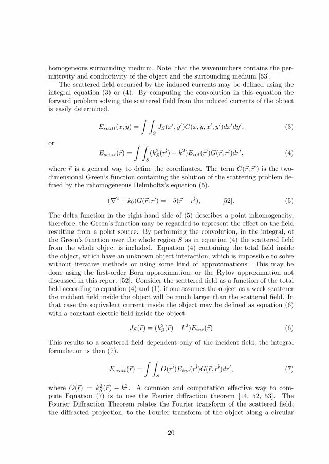
The scattered field occurred by the induced currents may be defined using theintegral equation (3) or (4). By computing the convolution in this equation theforward problem solving the scattered field from the induced currents of the objectis easily determined.

Escatt(x, y) =∫ ∫

S

JS(x′, y′)G(x, y, x′, y′)dx′dy′, (3)

orEscatt(~r) =

∫ ∫S

(k2S(~r′)− k2)Etot(~r′)G(~r, ~r′)dr′, (4)

where ~r is a general way to define the coordinates. The term G(~r, ~r′) is the two-dimensional Green’s function containing the solution of the scattering problem de-fined by the inhomogeneous Helmholtz’s equation (5).

(∇2 + k0)G(~r, ~r′) = −δ(~r − ~r′), [52]. (5)

The delta function in the right-hand side of (5) describes a point inhomogeneity,therefore, the Green’s function may be regarded to represent the effect on the fieldresulting from a point source. By performing the convolution, in the integral, ofthe Green’s function over the whole region S as in equation (4) the scattered fieldfrom the whole object is included. Equation (4) containing the total field insidethe object, which have an unknown object interaction, which is impossible to solvewithout iterative methods or using some kind of approximations. This may bedone using the first-order Born approximation, or the Rytov approximation notdiscussed in this report [52]. Consider the scattered field as a function of the totalfield according to equation (4) and (1), if one assumes the object as a week scattererthe incident field inside the object will be much larger than the scattered field. Inthat case the equivalent current inside the object may be defined as equation (6)with a constant electric field inside the object.

JS(~r) = (k2S(~r)− k2)Einc(~r) (6)

This results to a scattered field dependent only of the incident field, the integralformulation is then (7).

Escatt(~r) =∫ ∫

S

O(~r′)Einc(~r′)G(~r, ~r′)dr′, (7)

where O(~r) = k2S(~r) − k2. A common and computation effective way to com-

pute Equation (7) is to use the Fourier diffraction theorem [14, 52, 53]. TheFourier Diffraction Theorem relates the Fourier transform of the scattered field,the diffracted projection, to the Fourier transform of the object along a circular

20

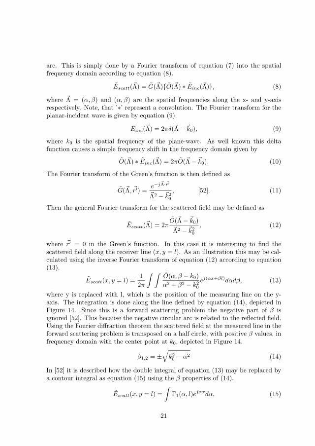
arc. This is simply done by a Fourier transform of equation (7) into the spatialfrequency domain according to equation (8).

Escatt(~Λ) = G(~Λ){O(~Λ) ∗ Einc(~Λ)}, (8)

where ~Λ = (α, β) and (α, β) are the spatial frequencies along the x- and y-axisrespectively. Note, that ’∗’ represent a convolution. The Fourier transform for theplanar-incident wave is given by equation (9).

Einc(~Λ) = 2πδ(~Λ− ~k0), (9)

where k0 is the spatial frequency of the plane-wave. As well known this deltafunction causes a simple frequency shift in the frequency domain given by

O(~Λ) ∗ Einc(~Λ) = 2πO(~Λ− ~k0). (10)

The Fourier transform of the Green’s function is then defined as

G(~Λ, ~r′) =e−j~Λ·~r′

~Λ2 − ~k20

, [52]. (11)

Then the general Fourier transform for the scattered field may be defined as

Escatt(~Λ) = 2πO(~Λ− ~k0)~Λ2 − ~k2

0

, (12)

where ~r′ = 0 in the Green’s function. In this case it is interesting to find thescattered field along the receiver line (x, y = l). As an illustration this may be cal-culated using the inverse Fourier transform of equation (12) according to equation(13).

Escatt(x, y = l) =12π

∫ ∫O(α, β − k0)α2 + β2 − k2

0

ej(αx+βl)dαdβ, (13)

where y is replaced with l, which is the position of the measuring line on the y-axis. The integration is done along the line defined by equation (14), depicted inFigure 14. Since this is a forward scattering problem the negative part of β isignored [52]. This because the negative circular arc is related to the reflected field.Using the Fourier diffraction theorem the scattered field at the measured line in theforward scattering problem is transposed on a half circle, with positive β values, infrequency domain with the center point at k0, depicted in Figure 14.

β1,2 = ±√

k20 − α2 (14)

In [52] it is described how the double integral of equation (13) may be replaced bya contour integral as equation (15) using the β properties of (14).

Escatt(x, y = l) =∫

Γ1(α, l)ejαxdα, (15)

21

where l must be larger than the object size and Γ1(α; l) is defined as

Γ1(α; l) =O(α,

√k20 − α2 − k0)

j2√

k20 − α2

ej√

k20−α2l. (16)

By taking the Fourier transform of both sides of equation (15) it results in equation(17). ∫

Escatt(x, y = l)ejαxdx = Γ1(α, l), (17)

where the Γ1(α, l) may be seen as a phase-shifted version of the object function O.Therefore, the Fourier transform of the scattered field along the measuring line aty = l is related to the Fourier transform of the object function along a circular arc.This technique is called Fourier Diffraction Projection Theorem [54]. For simplicity

Figure 14: The Fourier diffraction theorem, [52].

only one incidence angle is issued in this document, but for further informationabout multiple incidence see [53]. This theorem proves the validity of the relationbetween weakly scattering objects and the field measured at a line. Furthermore, In[54] two different types of algorithms are presented to solve the inverse problem toestimate the object, the filtered-backpropagation algorithm and using interpolationin both frequency and spatial domain. To the author’s knowledge the filtered-backproagation technique is the most commonly used, e.g. the planar microwavecamera by Bolomey et al. [16]. This algorithm is not given in detail here but theoverall principle with the filtered-backpropagation is described shortly. The filtered-backpropagation algorithm is very similar to the backpropagation algorithm for X-rays with the difference of an extra depth dependent filtering function. This filteringfunction is a transfer function corresponding to the depth depending attenuation

22

of the microwave. By using proper filter coefficients the received field may bebackpropagated to illustrate the object in slices parallel to the measuring line [54].

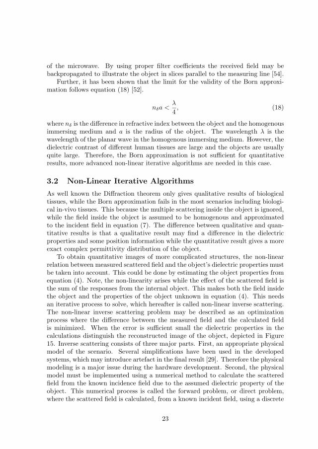
Further, it has been shown that the limit for the validity of the Born approxi-mation follows equation (18) [52].

nδa <λ

4, (18)

where nδ is the difference in refractive index between the object and the homogenousimmersing medium and a is the radius of the object. The wavelength λ is thewavelength of the planar wave in the homogenous immersing medium. However, thedielectric contrast of different human tissues are large and the objects are usuallyquite large. Therefore, the Born approximation is not sufficient for quantitativeresults, more advanced non-linear iterative algorithms are needed in this case.

3.2 Non-Linear Iterative Algorithms

As well known the Diffraction theorem only gives qualitative results of biologicaltissues, while the Born approximation fails in the most scenarios including biologi-cal in-vivo tissues. This because the multiple scattering inside the object is ignored,while the field inside the object is assumed to be homogenous and approximatedto the incident field in equation (7). The difference between qualitative and quan-titative results is that a qualitative result may find a difference in the dielectricproperties and some position information while the quantitative result gives a moreexact complex permittivity distribution of the object.

To obtain quantitative images of more complicated structures, the non-linearrelation between measured scattered field and the object’s dielectric properties mustbe taken into account. This could be done by estimating the object properties fromequation (4). Note, the non-linearity arises while the effect of the scattered field isthe sum of the responses from the internal object. This makes both the field insidethe object and the properties of the object unknown in equation (4). This needsan iterative process to solve, which hereafter is called non-linear inverse scattering.The non-linear inverse scattering problem may be described as an optimizationprocess where the difference between the measured field and the calculated fieldis minimized. When the error is sufficient small the dielectric properties in thecalculations distinguish the reconstructed image of the object, depicted in Figure15. Inverse scattering consists of three major parts. First, an appropriate physicalmodel of the scenario. Several simplifications have been used in the developedsystems, which may introduce artefact in the final result [29]. Therefore the physicalmodeling is a major issue during the hardware development. Second, the physicalmodel must be implemented using a numerical method to calculate the scatteredfield from the known incidence field due to the assumed dielectric property of theobject. This numerical process is called the forward problem, or direct problem,where the scattered field is calculated, from a known incident field, using a discrete

23

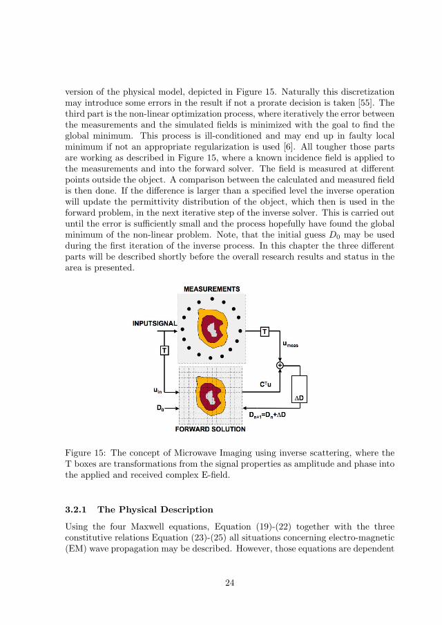
version of the physical model, depicted in Figure 15. Naturally this discretizationmay introduce some errors in the result if not a prorate decision is taken [55]. Thethird part is the non-linear optimization process, where iteratively the error betweenthe measurements and the simulated fields is minimized with the goal to find theglobal minimum. This process is ill-conditioned and may end up in faulty localminimum if not an appropriate regularization is used [6]. All tougher those partsare working as described in Figure 15, where a known incidence field is applied tothe measurements and into the forward solver. The field is measured at differentpoints outside the object. A comparison between the calculated and measured fieldis then done. If the difference is larger than a specified level the inverse operationwill update the permittivity distribution of the object, which then is used in theforward problem, in the next iterative step of the inverse solver. This is carried outuntil the error is sufficiently small and the process hopefully have found the globalminimum of the non-linear problem. Note, that the initial guess D0 may be usedduring the first iteration of the inverse process. In this chapter the three differentparts will be described shortly before the overall research results and status in thearea is presented.

Figure 15: The concept of Microwave Imaging using inverse scattering, where theT boxes are transformations from the signal properties as amplitude and phase intothe applied and received complex E-field.

3.2.1 The Physical Description

Using the four Maxwell equations, Equation (19)-(22) together with the threeconstitutive relations Equation (23)-(25) all situations concerning electro-magnetic(EM) wave propagation may be described. However, those equations are dependent

24

of both the E- and H- field. By taking the curl of both sides of Equation (19) or(20) and the using suitable constitutive relations it is possible to calculate the waveequation dependent on only one field component, the E- or H-field [56, 57].

∇×H = J +∂D

∂t(19)

∇× E = −∂B

∂t(20)

∇ ·D = ρ (21)∇ ·B = 0 (22)

J = σE (23)D = εE (24)B = µH (25)

The Maxwell’s equations describe the field properties in all three dimensions, whichresults in a calculation heavy vectorial problem in 3-D. By knowing the scenariomany simplification may be done to the final wave equation, e.g. if the incidencefield is vertically polarized and the object is homogenous along the z-axis. In thiscase the Maxwell’s equations may be simplified to the scalar Helmholtz equation(26), which is used in most of the developed systems [4, 5, 6, 15, 20, 23, 58].

(∇2 − k2(r))E(r) = 0, (26)

where k is called the wave number containing the material properties of the mediumthe EM-wave is propagating trough. E(x, y) is the total electric field. Other sim-plifications may be done by concerning the scenario as an infinite container with ahomogenous immersing medium. In this case the infinite boundary conditions ofthe Maxwell’s equation dramatically simplifies the solution of the wave equation[33].

3.2.2 The Forward Solution

The usual methods for the forward solver is the integral equation using Methodof Moments (MoM) [4, 5, 6, 15, 58], Finite Element Method (FEM) [22, 23, 25]orin some cases Finite Difference Method (FDM) [35, 59, 45]. This document willfocus on the may be most commonly used method in the literature, the integralformalization using MoM. This method were successfully used by several groups inparallel [4, 6, 58]. Those solutions are similar where the scenario where consideredto accomplish the scalar Helmholtz equation (26). The solution may be expressedby the integral equation (4). The discretization of the integral equation (4) is doneusing MoM [56, 6, 5], which results in equation (27), defining the relation between

25

the total field in the object and the measured scattered field.

Evscatt(rm) =

N∑j=1

(k2S(rj)− k2)Ev

tot(rj)G(rm, rj), m = 1, 2, · · ·,M, (27)

where M is the number of measurement points around the object and N is thenumber of discrete cells in the solution. The term v indicates the projection of thetransmitting antenna [6]. The total electric field inside the object ,from the N cells,is the solution of the linear system in

Evinc(rn) =

N∑j=1

[δnj − (k2S(rj)− k2)G(rm, rj)]Ev

tot(rj). n = 1, 2, · · ·, N, (28)

These two equations may be written in matrix form as equation (29) and (30).

[Evscatt] = [K][D][Ev

tot], (29)

[Evinc] = [I −GD][Ev

tot], (30)

where [Evscatt] is a vector with length M while [Ev

tot] and [Evinc] are vectors with

length N . The [D] matrix is an N x N diagonal matrix containing the permittiv-ity contrast of the N cells. The [K] and [G] matrix contains the Green’s operatorand have the sizes of M x N and N x N respectively. This technique works withthe discrete version of the exact integral equation, which is normally is a accuratemethod if the boundary conditions are selected properly. The FEM and FDM so-lutions are sometimes called differential methods, which builds on approximationswith local support while the integral formalization have global support [56]. Theproblem with integral formulations may be to define exact boundary conditions insome conditions, but in the case of microwave imaging often a infinity approxima-tion is used in the Green function. In this case the MoM solution is simple and havethe big advantage that only the object region has to be discretizised. However, thedifference between the methods will not be issued in detail in this document, theinterested reader may found it in literature such as [56].

3.2.3 The Inverse Optimization Process

The optimization process of the non-linear inverse scattering problem is a ill-posedproblem without only one simple solution. The key point is to minimize the errorbetween the measured and calculated field at the receiving antennas using a non-linear least square method, depicted in Figure 15. One may specify an objectfunction F as equation (31), which is the square norm of the difference between themeasured and calculated field shown in Figure 15.

F (D) =||Escatt(D)− Emeas||2

2= min, (31)

26

where the residual Escatt(D) − Emeas may be defined as ∆Escatt(D). The termD is the permittivity distribution matrix used in the forward solver as depictedin Figure 15. The goal is then to find the global minimum of this object functionusing the non-linear least-mean-square method. In the a general non-linear least-mean-square method,the Newton method, where both the gradient and the Hessianmatrix of the object function needs to be defined [60].The gradient of the objectfunction may be calculated as Equation (32) and the Hessian matrix as Equation(33).

∇DF (D) = JTF (D)∆Escatt(D) (32)

HF (D) = JTF (D)JF (D) +

M∑i=0

∆Eiscatt(D)H∆Ei

scatt(D), (33)

where M is the number of observation points. The optimization is located at theminimum point when the statement in Equation (34) is approved [60].

HF (D)∆s = −∇DF (D), (34)

where ∆s is the optimization step of the material property matrix D. The Hessianmatrix defined in Equation (33) is computation heavy and it is not efficient to cal-culate M H∆Ei

scatt(D) hessian matrixes in practical problems. Therefore equation

(34) is often simplified by using a Gauss-Newton method as

JTF (D)JF (D)∆s = −JT

F (D)∆Escatt(D). (35)

This solution is very limited while the implementation does not support regulariza-tion to avoid local minima of the object function. While this non-linear problem isill-posed the optimization needs to be controlled by regularization to suppress un-wanted results in local minima with non-realistic permittivity distribution. There-fore the Levenberg-Marquardt method [1, 5, 6], (this technique is also named theNewton-Kantorovich method [5, 7]), is often used in the literature . In these tech-niques the Hessian approximation is extended from the Gauss-Newton , defined asEquation (36). (

JTF (D)JF (D) + µI

)∆s = −JT

F (D)∆Escatt(D), (36)

where µ is often called the regularization-term used to improve the convergence ofthe ill-possed problem. This term is selected to improve the condition number of theJacobian matrix JT J , which stabilizes the convergence of the minimization of theobject function. Large regularization-term will filter out and suppress solutions withtoo rapid spatial variations in the material properties. Too large regularization-termwill of course limit the resolution around a high permittivity gradient inside theobject. Therefore, the regularization of the optimization is a major issue duringthe non-linear inverse scattering in microwave imaging.

27

3.2.4 The Development of the Non-Linear Inverse Scattering in Mi-crowave Imaging

The first non-linear inverse scattering solution where developed by different groupsin parallel in the beginning of the 90s. [4, 6, 58]. All these solutions use similarintegral formalization to express the scattered field in a infinite chamber. MoMis used in all cases to discretizise the investigation area of the forward problem.One slight difference between the solutions is that Chew et al. and Carosi et al.used the equivalent current formalization inside the object in the integral equa-tion of the scattered field similar to equation (3), while Joachimowicz et al. andFranchois et al. separated the E-field and the permittivity distribution to highlightthe permittivity distribution according to equation (4) and (27). All these solutionsused a Levenberg-Marquardt formulation of the inverse optimization problem, whileChew et al. and Carosi et al. call the solution Distorted Born and Nadine et al. calltheir solution for Newton-Kantorovich. In [5] it is shown that both Distorted Bornand Newton-Kantorovich is similar to the Levenberg-Marquardt solution. Differentkinds of regularization have been proposed but it is shown that the empiricallyTikkonov regularization offers the best results during high contrast objects wherethe initial guess differs a lot from the final unknown distribution. Further, thesesolutions are working with the scattered field, according to equation (37).

Escatt = Etot − Einc (37)

In practical measurements this means that first the field without the object ismeasured before the object is introduced int the scenario. Then the total field ismeasured including the object. Using equation (37) the measured scattered fieldfrom the object is calculated. Note, this is a differential measurement, which hasthe advantages to suppress offsets in the system and high-levels of incident field atantenna locations where the incidence field is much larger then the scattered field.Both those advantages will increase the sensitivity of the system.

In the middle of the 90s Meaney et al. proposed a Newton-type algorithmquite different to the earlier contributions. They were using the same Levenberg-Marquardt type of optimization with a Tikkonov regularization, but using a hybridelement forward solver instead of the earlier MoM contributions. The hybrid ele-ment (HE) solution contains of an FE mesh of the investigation area and a boundaryelement solution of the homogenous region outside the object. The FE method isknown to be an efficient way to model inhomogeneous dielectric objects with highspatial resolution, while sparse matrixes are used in the calculations. The processorload and memory usage are reduced compared to the integral formalization withMoM in many cases. The drawback is then that the whole scenario has to be dis-cretetisized compared to MoM where only the object region may be included. Oneeffective way to solve this is to use the Hybrid Element (HE) method, depicted inFigure 16. The idea is to use the FE method inside the object region and use aBE integral solution of the surrounding external medium [22][23]. However, in this

28

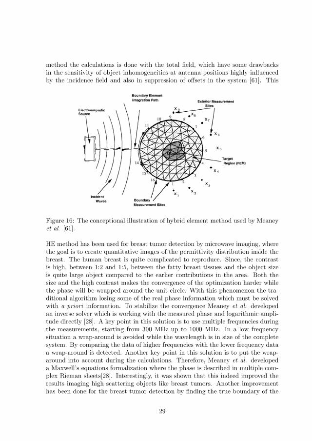
method the calculations is done with the total field, which have some drawbacksin the sensitivity of object inhomogeneities at antenna positions highly influencedby the incidence field and also in suppression of offsets in the system [61]. This

Figure 16: The conceptional illustration of hybrid element method used by Meaneyet al. [61].

HE method has been used for breast tumor detection by microwave imaging, wherethe goal is to create quantitative images of the permittivity distribution inside thebreast. The human breast is quite complicated to reproduce. Since, the contrastis high, between 1:2 and 1:5, between the fatty breast tissues and the object sizeis quite large object compared to the earlier contributions in the area. Both thesize and the high contrast makes the convergence of the optimization harder whilethe phase will be wrapped around the unit circle. With this phenomenon the tra-ditional algorithm losing some of the real phase information which must be solvedwith a priori information. To stabilize the convergence Meaney et al. developedan inverse solver which is working with the measured phase and logarithmic ampli-tude directly [28]. A key point in this solution is to use multiple frequencies duringthe measurements, starting from 300 MHz up to 1000 MHz. In a low frequencysituation a wrap-around is avoided while the wavelength is in size of the completesystem. By comparing the data of higher frequencies with the lower frequency dataa wrap-around is detected. Another key point in this solution is to put the wrap-around into account during the calculations. Therefore, Meaney et al. developeda Maxwell’s equations formalization where the phase is described in multiple com-plex Rieman sheets[28]. Interestingly, it was shown that this indeed improved theresults imaging high scattering objects like breast tumors. Another improvementhas been done for the breast tumor detection by finding the true boundary of the

29

breast before setting the hybrid element solution of the scenario. This is done byconformal microwave imaging [2]. The boundary between the FE method and theBoundary Element region is located to the boundary of the breast. In this moveit is possible to set a step function at the boundary with the permittivity of thesurrounding water. When the permittivity of the background medium is knownthe inverse problem includes only to find the permittivity of the object itself. Thisimproved the quantitative result a lot, especially when the tumor was located nearthe boundary of the breast [2]. The first HE algorithm did not integrate the in-teraction of the antennas and the surrounding system, as the first MoM solutionsbut some effort has been done to take the nonactive antennas into account [62, 63].The resulting model of the nonactive antenna is a microwave-sinc, which suppressesthe wave without any reflections. Also, the MoM solvers like Newton-Kantorovitchhave been improved with the interaction of the antenna coupling [64]. With thissolution it is possible to use a non lossy medium and create images without theinfinite approximation of the scenario.

Alternative optimizing schemes have also been investigated, the MultiplicativeRegularization Contrast Source inversion by Abubakar et. al.[67, 69, 71], global op-timization methods using neural networks, genetic algorithms and nondestructiveevaluation by Caorsi et. al. [72, 73, 74, 75]. Those methods will not be issued inthis report, but in shortly those methods avoiding local minima though the globaloptimization with the cost of a slower convergence and higher computation load.Until now single frequency solutions is most widely used, but different groups work-ing on multi-frequency solutions [45, 46, 76]. It is known that the low frequencieslower the affect of non-linearities and stabilizes the algorithm, while the higher fre-quencies increasing the resolution, the idea is that a combination will improve thereconstruction. However, there is a frequency dependence of biological tissues andmany future research efforts could focus in this area.

30

4 The Phantom Model Development

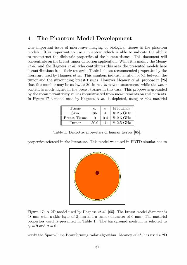
One important issue of microwave imaging of biological tissues is the phantommodels. It is important to use a phantom which is able to indicate the abilityto reconstruct the dielectric properties of the human tissues. This document willconcentrate on the breast tumor detection application. While it is mainly the Meanyet al. and the Hagness et al. who contributes this area the presented models hereis contributions from their research. Table 1 shows recommended properties by theliterature used by Hagness et al.. This numbers indicate a ration of 5:1 between thetumor and the surrounding breast tissues. However Meaney et al. propose in [25]that this number may be as low as 2:1 in real in vivo measurements while the watercontent is much higher in the breast tissues in this case. This propose is groundedby the mean permittivity values reconstructed from measurements on real patients.In Figure 17 a model used by Hagness et al. is depicted, using ex-vivo material

Tissue εr σ FrequencySkin 36 4 @ 2.5 GHz

Breast Tissue 9 0.4 @ 2.5 GHzTumor 50.0 4 @ 2.5 GHz

Table 1: Dielectric properties of human tissues [65].

properties refereed in the literature. This model was used in FDTD simulations to

Figure 17: A 2D model used by Hagness et al. [65]. The breast model diameter is68 mm wich a skin layer of 2 mm and a tumor diameter of 6 mm. The materialproperties used is presented in Table 1. The background medium is selected toεr = 9 and σ = 0.

verify the Space-Time Beamforming radar algorithm. Meaney et al. has used a 2D

31

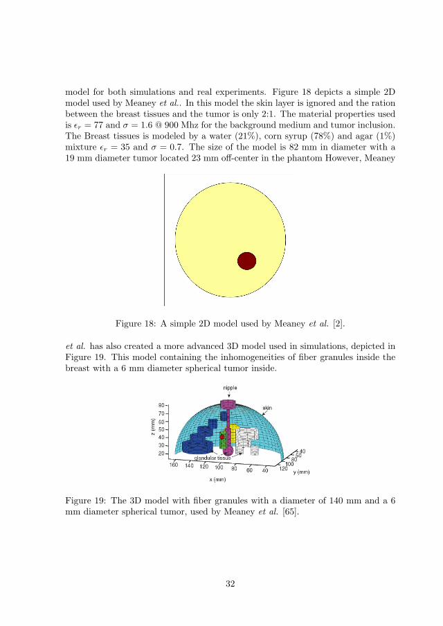
model for both simulations and real experiments. Figure 18 depicts a simple 2Dmodel used by Meaney et al.. In this model the skin layer is ignored and the rationbetween the breast tissues and the tumor is only 2:1. The material properties usedis εr = 77 and σ = 1.6 @ 900 Mhz for the background medium and tumor inclusion.The Breast tissues is modeled by a water (21%), corn syrup (78%) and agar (1%)mixture εr = 35 and σ = 0.7. The size of the model is 82 mm in diameter with a19 mm diameter tumor located 23 mm off-center in the phantom However, Meaney

Figure 18: A simple 2D model used by Meaney et al. [2].

et al. has also created a more advanced 3D model used in simulations, depicted inFigure 19. This model containing the inhomogeneities of fiber granules inside thebreast with a 6 mm diameter spherical tumor inside.

Figure 19: The 3D model with fiber granules with a diameter of 140 mm and a 6mm diameter spherical tumor, used by Meaney et al. [65].

32

Those examples are the mainly contributions in the phantom area of breasttumor detection. The exact in-vivo complex permittivity seems to be not settledyet while the properties variate between different patients with different blood flow,different age and rate of fatty tissue inside the breast. However a expected contrastbetween 1.5-5:1 seems to be settled [50].

5 Discussion and Future Work

Imaging of biological tissues is one of the most challenging application area ofmicrowave imaging. This is mostly because of the high permittivity contrast ofbiological tissues and the complex geometrical structure. In many industrial appli-cation the diffraction tomography using the Born approximation is well suited withits computational effectiveness. However, in the most cases of biological imagingthe non-linear multiple scattering inside the object must be taken into account.Because, the size and contrast are to big to appropriately use the Born approx-imation. Several groups have put a lot of effort to solve the ill-posed non-linearinverse problem. The other approach, using radar techniques the detection andlocalization of strong scatters are possible. However, while the author believe thatthe quantitative complex permittivity reconstruction may be useful in the decisione.g. if the tumor is malign, the iterative non-linear inverse scattering solution ispreferred.

At the moment mostly 2D slices in the TM-case have been investigated. Someapproaches have been done to use a scalar 3D algorithm in a TM-wave system,by Meaney et al. Also Semenov et al. have tried to produce 3D solutions using avectorial 3D algorithm with promising results. In the authors opinion, it could beinteresting to use the Newton-Kantorovich based on MoM in the breast tumor case,to se the usability of these algorithms in this area. By transform the algorithm tothe 2.45 GHz planar microwave camera located at Supelec as Ann Franchois, furtherquantitative investigations may be done of inhomogeneous objects. While the retinaof the planar camera measures the vertical electric field, it may be useful in the3D case by rotating the retina 90 degrees measuring both vertical and horizontalpolarized E-field. The earlier 2D system developed by Meaney textitet al. suffersfrom several 3D/2D artifacts. By using the planar camera in 3D configurationfurther 3D investigation may be done.

6 Conclusions

In this document the historical development of the biomedical imaging using mi-crowaves is issued. Several hardware systems have been developed with differentaims some more successful than others. However, the main issue of this documentis the application of breast tumor detection using microwave imaging. In this areait is mainly two groups with active research, Meaney et al. and Hagness et al..

33

They have complectly different approach around the problem where Meaney et al.using nonlinear microwave tomography to create quantitative permittivity images,while Hagness et al. tries to find the tumor using radar techniques. The radarapproach may be useful while it may be easier to realize as a clinical system fordetection and positioning of the tumor more easily, but it may not be able to createpermittivity information about the scatterer it self, i.e. if the tumor is malign ornot. Therefore, the author indicates the interest to further develop the microwavetomography for this purpose. The system today uses 2-D models for the imagingpurpose. The more calculation loaded 3-D case is therefore of interest. By applyingthe non-linear inverse scattering to a modified planar microwave camera, locatedat Supelec, fully 3-D investigation may be performed.

34

References

[1] Q. Fang, P. M. Meaney, S. D. Geimer and A. V. Streltsov, “Microwave ImageReconstruction From 3-D Fields Coupled to 2-D Parameter Estimation,” IEEETransactions on Medical Imaging, Vol-23, No. 4, pp. 475–484, April 2004.

[2] D. Li, P. MMeaney and K. D. Paulsen, “Conformal Microwave Imaging forBreast Cancer Detection,” IEEE Transactions on Mircorwave Theory andTechniques, Vol-51, No. 4, pp. 1179–1186, April 2003.

[3] P. M. Meaney, Q. Fang, E. Demidenko and K. D. Paulsen, “Error Analysis inMicrowave Breast Imaging: Variance Stabilizing Transformations,” Procedingcof ICONIC 2005, UPC Barcelona, Spain, pp. 67–71, June 2005.

[4] W. C. Chew and Y. M. Wang,”Reconstruction of Two-Dimensional Permittiv-ity Distribution Using the Distorted Born Iterative Method,” IEEE Transac-tions on Medical Imaging, Vol-9, No. 2, pp. 218–225, April 2004.

[5] A. Franchois, C. Pichot”Microwave Imaging–Complex Permittivity Recon-struction with a Levenberg-Marquardt Method,” IEEE Transactions on An-tennas and Propagation, Vol-45, No. 2, pp. 203–215, February 1997.

[6] N. Joachimowicz, C. Pichot and J. -P. Hugonin, “Inverse Scattering: An Itera-tive Numerical Method for Electromagnetic Imaging,” IEEE Transactions onAntennas and Propagation, Vol-395, No. 12, pp. 1742–1752, December 1991.

[7] N. Joachimowicz, J. J. Mallorqui, J. -C. Bolomey and A. Broquetas, “Conver-gence and Stability Assessment of Newton–Kantorovich Reconstruction Algo-rithms for Microwave Tomography,” IEEE Transactions on Medical Imaging,Vol-17, No. 4, pp. 562–570, August 1998.

[8] A. E. Bulyshev, A. E. Souvorov, S. Y. Semenov, V. G. Posukh and Y. E. Sizov,“Three-dimensional vector microwave tomography theory and computationalexperiments,” Institute of Physics Publishing, Inverse Problems, No. 20, PII:S0266-5611(04)72896-8, pp. 1239–1259, 2004.

[9] A. Abubakar, P. M. van den Berg and S. Y. Semenov, “Two- and Three-Dimensional Algorithms for Microwave Imaging and Inverse Scattering,” Jour-nal of Electromagnetism Waves and Applications, Vol-17, No. 2, pp. 209–231,2003.

[10] L. E. Larsen and J. H. Jacobi, “Mcrowave Scattering Parameter Imaging odan Isolated Canine Kidney,” Medical Physics, Vol-6, pp. 394–403, 1979.

[11] Bolomey J. C. Gardiol Fred E. “Engineering Applications of the ModulatedScatterer Technique”, [Series: Artech House Antennar and Propagation Li-brary], ISBN: 1580531474.

35

[12] A. Joisel, J. Mallorqui, A. Broquetas, J. M. Geffrin, N. Joachimowicz, M.V. Iossera, L. Jofre and J. -C. Bolomey, “Microwave Imaging Techniques forBiomedical Applications,” Instrumentation and Measurement Technology Con-ference, 1999.

[13] J. -C. Bolomey, L. Jofre and G. Peronnet “On the Possible Use of Microwave-Active Imaging for Remote Thermal Sensing,” IEEE Transactions on Mircor-wave Theory and Techniques, Vol-31, No. 9, pp. 777–781, September 1983.

[14] C. Rius, C. Pichot, L. Jofre, J. -C. Bolomey, N. Joachimowicz, A. Broque-tas and M. Ferrando, “Planar and Cylindrical Active Microwave TemperatureImaging: Numerical Simulations,” IEEE Transactions on Medical Imaging,Vol-11, No. 4, pp. 457–469, December 1992.

[15] A. Franchois, A. Joisel, C. Pichot and J. -C. Bolomey, “Quantitative MicrowaveImaging with a 2.45-GHz Planar Microwave Camera,” IEEE Transactions onMedical Imaging, Vol-17, No. 4, pp. 550–561, August 1998.

[16] A. Joisel and J. -C. Bolomey, “Rapid Microwave Imaging of Living Tissues,”SPIE Symposium on Medical Imaging San Diego, CA, USA, February 12-18,2000.

[17] L. Jofre, M. S. Hawley, A. Broquetas, E. De Los Reyes, M. Ferrando and A.R. Elias-Fuste, “Medical Imaging with a Microwave Tomographic Scanner,”IEEE Transactions on Biomedical Engineering, Vol-37, No. 3, pp. 303–311,March 1990.

[18] A. Broquetas, J. Romeu, J. M. Rius, A. R. Elias-Fuste, A. Cardama and L.Jofre, “Cylindrical Geometry: A Further Step in Active Microwave Tomogra-phy,” IEEE Transactions on Mircorwave Theory and Techniques, Vol-39, No.5, pp. 836–844, May 1991.

[19] A. Abubakar, P. M. van den Berg and J. J. Mallorqui, “Imaging of BiomedicalData Using a Multiplicative Regularized Contrast Source Inversion Method,”IEEE Transactions on Mircorwave Theory and Techniques, Vol-50, No. 7, pp.1761–1771, July 2002.

[20] S. Y. Semenov, R. H. Svenson, A. E. Boulyshev, A. E. Souvorov, V. Y. Borisov,Y. Sizov, A. N. Starostin, K. R. Dezern, G. P. Tatsis and V. Y. Baranov,“Microwave Tomography: Two-Dimensional System for Biomedical Imaging,”IEEE Transactions on Biomedical Engineering, Vol-43, No. 9, pp. 869–877,September 1996.

[21] P. M. Meaney, K. D. Paulsen, A. Hartov and R. K. Crane, “An Actice Mi-crowave Imaging System for Reconstruction of 2-D Electrical Property Distri-butions,” IEEE Transactions on Biomedical Engineering, Vol-42, No. 10, pp.1017–1025, October 1995.

36

[22] P. M. Meaney, K. D. Paulsen and T. P. Ryan, “Two-Dimensional HybridElement Image reconstruction for TM Illumination,” IEEE Transactions onAntennas and Propagation, Vol-43, pp. 239–247, 1995.

[23] K. D. Paulsen, P. M. Meaney, M. J. Moskowitz and J. M. Sullivan, “A DualMesh Scheme for Finite Element Based Reconstruction Algorithms,” IEEETransactions on Medical Imaging, Vol-14, No. 3, pp. 504–514, Mars 1995.

[24] P. M. Meaney, K. D. Paulsen and J. T. Chang, “Near-Field Microwave Imagingof Biologically-Based Materials Using a Monopole Trenceiver System,” IEEETransactions on Mircorwave Theory and Techniques, Vol-46, No. 1, pp. 31–43,January 1998.

[25] P. M. Meaney, M. W. Fanning, D. Li, S. P. Poplack and K. D. Paulsen, “AClinical Prototype for Active Microwave Imaging of the Breast,” IEEE Trans-actions on Mircorwave Theory and Techniques, Vol-48, No. 11, pp. 1841–1853,November 2000.

[26] K. D. Paulsen, P. M. Meaney, “Nonactive Antenna Compensation for Fixed-Array Microwave Imaging–Part I: Model Development”, IEEE Transactionson Medical Imaging, Vol. 18, pp. 496–507, June 1999.

[27] P. M. Meaney, K. D. Paulsen, J. T. Chang, M. W. Fanning, and A. Hartov,“Nonactive Antenna Compensation for Fixed-Array Microwave Imaging PartII:–Imaging Results”, IEEE Transactions on Medical Imaging, Vol. 18, pp.508–518, June 1999.

[28] P. M. Meaney, K. D. Paulsen, B. W. Pogue and M. I. Miga, “Microwave ImageReconstruction Utilizing Log-Magnitude and Unwrapped Phase to ImproveHigh-Contrast Object Recovery,” IEEE Transactions on Medical Imaging, Vol-20, No. 2, pp. 104–116, February 2001.

[29] P. M. Meaney, K. D. Paulsen, S. D. Geimer, S. A. Haider and M. W. Fanning,“Quantification of 3-D Field Effects During 2-D Microwave Imaging,” IEEETransactions on Biomedical Engineering, Vol-49, No. 7, pp. 708–720, July2002.

[30] D. Li, P. M. Meaney, T. Raynolds, S. A. Pendergrass, M. W. Fanning and K. D.Paulsen, “A BROADBAND MICROWAVE BREAST IMAGING SYSTEM,”2003 IEEE 29th Annual Biomedical Conference, Proceeding of, pp. 83–84, Mars2003.

[31] J. M. Geffrin J. J. Mallorqui, N. Joachimowicz R. Redondo, M. Vall-Ilossera,O. Franza, A. Joisel and J. -C. Bolomey, “REDUCTION OF THE MODELNOISE IN NON-LINEAR RECONSTRUCTION VIA AN EFFICIENT CAL-CULATION OF THE INCIDENT FELD : APPLICATION TO A 434 MHz

37

SCANNER,” Antennas and Propagation Society 1999 IEEE InternationalSymposium, Vol-2, pp. 996–999, July 1999.

[32] J. M. Geffrin and A. Joisel, “Comparison of Measured and Simulated Incidentand Scattered Fields in a 434 Mhz Scanner,” Procedingc of the 22th URSIGeneral Asambly 2002, Maastricht, The Netherlands, 17-24 August 2002.

[33] A. Franchois and A. G. Tijhuis, “A Newton-Type Reconstruction Algorithmfor a 434 Mhz Microwave Imaging Scanner,” Procedingc of the 22th URSIGeneral Asambly 2002, Maastricht, The Netherlands, 17-24 August 2002.

[34] S. Caorsi, A. Massa and M. Pastorino, “A Numerical Solution to Full-VectorElectromagnetic Scattering by Three-Dimensional Nonlinear Bounded Di-electrics,” IEEE Transactions on Mircorwave Theory and Techniques, Vol-43,No. 2, pp. 1841–1853, February 1995.

[35] P. M. Meaney, Q. Fang, S. D. Geimer, A. V. Streltsov and K. D. Paulsen, “3DScalar Microwave Image Reconstruction Algorithm,” Microwave SymposiumDigest, 2002 IEEE MTT-S International, Vol-3, pp. 2269–2272, 2-7 June 2002.

[36] S. Y. Semenov, R. H. Svenson, A. E. Boulyshev, A. E. Souvorov, A. G.Nazarov, Y. E. Sizov, A. Pavlovsky, V. Y. Borisov, B. A. Voinov, G. I. Si-monova, A. N. Starostin, V. G. Posukh, M. Taran, G. P. Tatsis, and V. Y.Baranov, “Three-Dimensional Microwave Tomography: Experimental Proto-type of the System and Vector Born Reconstruction Method,” IEEE Transac-tions on Biomedical Engineering, Vol-46, No. 8, pp. 937–946, August 1999.

[37] S. Y. Semenov, R. H. Svenson, A. E. Boulyshev, A. E. Souvorov, V. Y. Borisov,A. G. Nazarov, Y. E. Sizov, V. G. Posukh, A. Pavlovsky, P. N. Repin, A. N.Starostin, B. A. Voinov, M. Taran, G. P. Tatsis, and V. Y. Baranov, “Three-Dimensional Microwave Tomography: Initial Experimental Imaging of Ani-mals,” IEEE Transactions on Biomedical Engineering, Vol-49, No. 1, pp. 55–63, January 2002.

[38] S. Y. Semenov, A. E. Boulyshev, A. E. Souvorov, A. G. Nazarov, Y. E. Sizov,R. H. Svenson, V. G. Posukh, A. Pavlovsky, P. N. Repin and G. P. Tatsis,“Three-Dimensional Microwave Tomography: Experimental Imaging of Phan-toms and Biologocal Objects,” IEEE Transactions on Microwave Theory andThechniques, Vol-48, No. 6, pp. 1071–1074, June 2000.

[39] S. Y. Semenov, R. H. Svenson, A. E. Boulyshev, A. E. Souvorov, A. G.Nazarov, Y. E. Sizov, V. G. Posukh, A. Pavlovsky, P. N. Repin and G. P.Tatsis, “Spatial Resolution of Microwave Tomography for Detection of Myocar-dial Ischemia and InfarctionExperimental Study on Two-Dimensional Models,”IEEE Transactions on Microwave Theory and Thechniques, Vol-48, No. 4, pp.538–544, April 2000.

38

[40] M. Miyakawa and T. Hayashi, ”An Atemt of High-Speed Imaging of the ChirpRadar-Type Microwave Computed Tomography,” Microwave Symposium Di-gest, 1997., IEEE MTT-S International, Vol-1, pp. 115–118, June 8-13, 1997.

[41] M. Miyakawa, E. Harada and W. Jing,”Chirip Pulse Microwave ComputedTomography(CP-MCT) Equipped with a Fan Beam Scanner for High-speedImaging of a Biological Target,” Proceedings of the 25 Annual lntemationalConference of the IEEE EMBS, Caneun, Mexico, September 17-21, 2003.

[42] M. Bertero, M. Miyakawa, P. Boccacci, F. Conte, K. Orikasa and M. Furutani,“Three-Dimensional Microwave Tomography: Initial Experimental Imaging ofAnimals,” IEEE Transactions on Biomedical Engineering, Vol-47, No. 5, pp.690–699, May 2000.

[43] M. Miyakawa, K. Orikasa, M. Bertero, P. Boccacci, F. Conte and M. Piana,“Experimental Validation of a Linear Model for Data Reduction in Chirp-PulseMicrowave CT,” IEEE Transactions on Medical Imaging, Vol-21, No. 4, pp.385–395, April 2002.

[44] M. Miyakawa, T. Ishida and M. Watanabe,”Imaging Capability of an EarlyStage Breast Tumor by CP-MCT,” Procedingc of the 26th Annual InternationalConference of the IEEE EMBS San Francisco, CA, USA, September 1-5, 2004.

[45] A. Fhager, P. Hashemzadeh, and M. Persson, ”Reconstruction Quality andSpectral Content of an Electromagnetic Time-Domain Inversion Algorithm”,IEEE Transactions on Biomedical Engineering, Vol-53, No. 8, pp. 1594–1604,August 2006.

[46] A. Fhager, “ Microwave Tomography,” Ph.D. Thesis, Department of Signalsand Systems, Chalmers Univerity of Technology, 2006.

[47] E. C. Fear, X. Li and S. C. Hagness, ”Confocal Microwave Imaging for BreastCancer Detection: Localization of Tumors in Three Dimensions,” IEEE Trans-actions on Biomedical Engineering, Vol-49, No. 8, pp. 812–822, August 2002.

[48] J. Bond, X. Li and S. C. Hagness ”Microwave Imaging via Space-Time Beam-forming for Early Detection of Breast Cancer,” IEEE Transactions on Anten-nas and Propagation, Vol-51, No. 8, pp. 1690–1705, August 2003.

[49] J. Bond, X. Li and S. C. Hagness ”Numerical and Experimental Investigationof an Ultrawideband Ridged Pyramidal Horn AntennaWith Curved LaunchingPlane for Pulse Radiation,” IEEE Antennas and Wireless Propagation Letters,Vol-2, pp. 259–262, 2003.

[50] X. Li, S. K. Davis, S. C. Hagness, D. W. van der Weide and B. D. Van Veen,”Microwave Imaging via SpaceTime Beamforming: Experimental Investigation

39

of Tumor Detection in Multilayer Breast Phantoms,” IEEE Transactions onMircorwave Theory and Techniques, Vol-52, No. 8, pp. 1856–1865, August2004.

[51] J. -C. Bolomey, A. Izadnegahdar, L. Jofre, C. Pichot, G. Peronnet and M.Solaimani, “Microwave Diffraction Tomography for Biomedical Applications,”IEEE Transactions on Mircorwave Theory and Techniques, Vol-30, No. 11, pp.1998–1982, November 1982.

[52] M. Slaney, A. C. Kak, and L. E. Larsen, “Limitations of Imaging with First-Order Diffraction Tomography,” IEEE Transactions on Mircorwave Theoryand Techniques, Vol-32, No. 8, pp. 860–874, August 1984.

[53] C. Pichot, L. Jofre, G. Peronnet and J. -C. Bolomey, “Active Microwave Imag-ing of Inhomogeneous Bodies,” IEEE Transactions on Antennas and Propaga-tion, Vol-33, No. 4, pp. 416–423, April 1985.

[54] S. X. Pan and A. C. Kak, “A Computational Study of Reconstruction Algo-rithms for Diffraction Tomography: Interpolation Versus Filtered Backpropa-gation,” IEEE Transactions on Acoustics, Speech and Signal Processing, Vol-31, No. 5, pp. 1262–1275, October 1983.

[55] N. Joachimowicz and C. Pichot, “Comparison of Three Integral Formulationsfor the 2-D TE scattering Problem,” IEEE Transactions on Mircorwave Theoryand Techniques, Vol-38, No. 2, pp. 178–184, February 1990.

[56] M. V. K. Chari, S. J. Salon, ”Numerical Methods in Electromagnetism, ”Academic Press, ISBN: 0-12-615760-X, 2000.

[57] R. F. Harrington, ”Time-Harmonic Electromagnetic Fields, ” IEEE Press,ISBN: 0-471-20806-X.

[58] S. Caorosi, G. L. Gragnani and M. Pastorino, “Two-Dimensional MicrowaveImaging by a Numerical Inverse Scattering Solution,” IEEE Transactions onMircorwave Theory and Techniques, Vol-38, No. 8, pp. 981–989, August 1990.

[59] W. C. Chew G. P. Otto, W. H. Weedon, J. H. Lin, Y. M. Wang and M. Moghad-dam, “Nonlinear Diffraction Tomography—The Use of Inverse Scattering forImaging,” Conference Record of The Twenty-Seventh Asilomar Conference onSignals, Systems and Computers, 1993., Vol-1, pp. 120–129, 1-3 November1993.

[60] M. T. Heath, ”Scientific Computing, ” Second Edition, Mc Graw Hill, ISBN:0-07-112229-X, 2002.

40

[61] P. M. Meaney, K. D. Paulsen, A. Hartov and R. K. Crane, “Microwave Imagngfr Tissue Assessment: Initial Evaluation in Multitarget Tissue-EquivalentPhantoms,” IEEE Transactions on Biomedical Engineering, Vol-43, No. 9, pp.878–890, September 1996.

[62] K. D. Paulsen and P. M. Meaney, “Nonactive Antenna Compensation forFixed-Array Microwave Imaging—Part I: Model Development,” IEEE Trans-actions on Medical Imaging, Vol-18, No. 6, pp. 496–506, June 1999.

[63] P. M. Meaney, K. D. Paulsen, J. T. Chang, M. W. Fanning and A. Hartov,“Nonactive Antenna Compensation for Fixed-Array Microwave Imaging: PartII—Imagng Results,” IEEE Transactions on Medical Imaging, Vol-18, No. 6,pp. 508–518, June 1999.

[64] O. Franza, N. Joachimowicz and J. -C. Bolomey, “SICS: A Sencor Interac-tion Compensation Scheme for Microwave Imaging,” IEEE Transactions onAntennas and Propagation, Vol-50, No. 2, pp. 211–216, February 2002.

[65] E. C. Fear, P. M. Meaney and M. A. Stuchly, “Microwaves for Breast CancerDetection,” IEEE Potentials, pp. 12–18, February 2003.

[66] A. E. Souvorov, A. E. Bulyshev, S. Y. Semenov, R. H. Svenson, A. G. Nazarov,Y. E. Sizov, and G. P. Tatsis, “Microwave Tomography: A Two-DimensionalNewton Iterative Scheme,” IEEE Trans. Microwave Theory and Tech., vol. 46,pp. 1654–1659 , Nov. 1998.

[67] S. Y. Semenov, A. E. Bulyshev, A. Abubakar, V. G. Posukh, Y. E. Sizov,A. E. Souvorov, P. M. van den Berg, and T. C. Williams, “Microwave-Tomographic Imaging of the High Dielectric-Contrast Objects Using Differ-ent Image-Reconstruction Approaches,” IEEE Trans. Microwave Theory andTech., vol. 53, pp. 2284–2294 , July 2005.

[68] A. E. Bulyshev, A. E. Souvorov, S. Y. Semenov, V. G. Posukh and Y. E. Sizov,“Three-dimensional vector microwave tomography: theory and computationalexperiments,” Inverse Problems, vol. 20, pp. 1239-1259, 2004.

[69] A. Abubakar P. M. van den Berg and S. Y. Semenov “TWO- AND THREE-DIMENSIONAL ALGORITHMS FOR MICROWAVE IMAGING AND IN-VERSE SCATTERING,” J. of Electromagn. Waves and Appl., Vol. 17, pp.209–231, 2003.

[70] S. Caorsi, A. Massa, and M. Pastorino “A Numerical Solution to Full-VectorElectromagnetic Scattering by Three-Dimensional Nonlinear Bounded Di-electrics,” IEEE Trans. Microwave Theory and Tech. , vol. 43, pp. 428–436, Feb. 2005.

41

[71] A. Abubakar, P. M. van den Berg, and J. J. Mallorqui “Imaging of BiomedicalData Using a Multiplicative Regularized Contrast Source Inversion Method,”IEEE Trans. Microwave Theory and Tech., vol. 50, pp. 1761–177 , Jul. 2005.

[72] S. Caorsi and P. Gamba, “Electromagnetic Detection of Dielectric Cylindersby a Neural Network Approach,” IEEE Trans. Geoscience Remote Sens., vol.37, pp. 820–827, Mar. 1999.

[73] M. Pastorino, A. Massa, and S. Caorsi, “A Microwave Inverse Scattering Tech-nique for Image Reconstruction Based on a Genetic Algorithm,” IEEE Trans.Instrumen. Measure., vol. 49, pp. 573–578, June 2000.

[74] M. Pastorino, S. Caorsi, A. Massa, and A. Randazzo, “Reconstruction Algo-rithms for Electromagnetic Imaging,” IEEE Trans. Instrumen. Measure., vol.53, pp. 692–699, June 2004.

[75] M. Pastorino, S. Caorsi, and A. Massa, “A Global Optimization Technique forMicrowave Nondestructive Evaluation,” IEEE Trans. Instrumen. Measure.,vol. 51, pp. 666–673, Aug. 2002.

[76] Q. Fang, P. M. Meaney, and K. D. Paulsen, “Microwave Image Reconstructionof Tissue Property Dispersion Characteristics Utilizing Multiple-Frequency In-formation,” IEEE Trans. Microwave Theory and Tech., vol. 52, pp. 1866–1875,Aug. 2004.

42