MICROWAVE COMMUNICATION“God chose the weak things of the world to shame the strong.”

1 Cor. 1:27

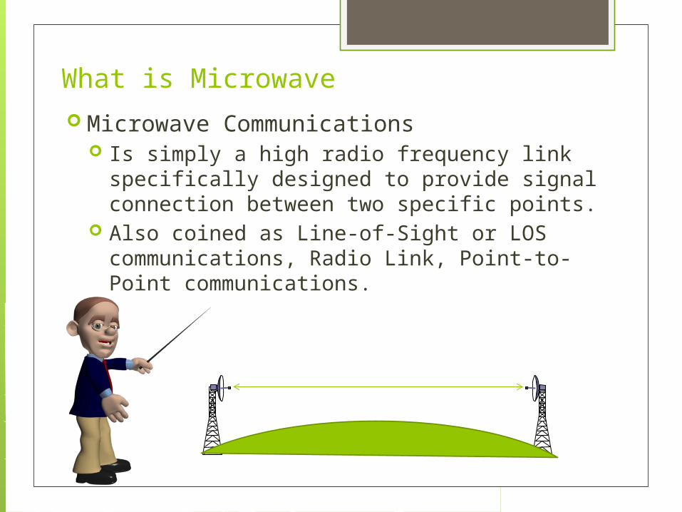
What is Microwave Microwave Communications

Is simply a high radio frequency link specifically designed to provide signal connection between two specific points.

Also coined as Line-of-Sight or LOS communications, Radio Link, Point-to-Point communications.

2

What is Microwave Communication A communication system that utilizes the

radio frequency band spanning 2 to 60 GHz. As per IEEE, electromagnetic waves between 30 and 300 GHz are called millimeter waves (MMW) instead of microwaves as their wavelengths are about 1 to 10mm.

Small capacity systems generally employ the frequencies less than 3 GHz while medium and large capacity systems utilize frequencies ranging from 3 to 15 GHz. Frequencies > 15 GHz are essentially used for short-haul transmission.

Microwave Communication3

3

Classification of Microwave Nature

Analog Digital

Distance / Frequency Short Haul

used for short distance microwave transmission usually at lower capacity ranging from 64 kbps up to 2Mbps

Medium Haul Long Haul

used for long distance/multi-hop microwave transmission. Used for backbone route applications at 34 Mbps to 620 Mbps capacity

Capacity / Bandwidth Light (Narrow Band) Medium (Narrow Band) Large (Wide Band)

4

Advantages of Microwave System The gain of an antenna is proportional to its

electrical size. A 1% bandwidth provides more frequency range

at microwave frequencies than that of HF. Microwave signals travel predominantly by LOS. There is much less background noise at

microwave frequencies than at RF. Microwave systems do not require a right-of-way

acquisition between stations. Fewer repeaters are necessary for amplification. Underground facilities are minimized. Increased reliability and less maintenance.

5

Disadvantage of Microwave System More difficult to analyze electronic circuits Conventional components (resistors, inductors, and capacitors)

cannot be used at microwave frequencies. There are physical limitations in creating resonant circuits at

microwave frequencies. Conventional semi-conductor devices do not work properly at

microwave frequencies because of Inherent inductances and capacitances of the terminal leads and Transit time

For amplification, vacuum tubes are used such as klystrons, magnetrons and traveling wave tubes (TWT).

Distance of operation is limited by line of sight (LOS). Microwave signals are easily reflected and/or diverted because of

the very short wavelength. Atmospheric conditions such as rain/fog can attenuate and absorb

the microwave signal especially at 20 GHz and up.6

Terrestrial Microwave Types Of Microwave Stations

Terminals – are points in the system where the baseband signals either originate or terminate

Repeaters – are points in the system where the baseband signals maybe reconfigured or simply repeated or amplified. Passive Microwave repeaters – a device that re-

radiates microwave energy without additional electronic power. back to back billboard type

Active Microwave repeater – a receiver and a transmitter placed back to back or in tandem with the system. It receives the signal, amplifies and reshapes it, then retransmits the signal to the next station. 7

The K-Curve A numerical figure that considers the non-ideal condition of

the atmosphere refraction that causes the ray beam to be bent toward the earth or away from the earth.

o

e

r

rk

RadiusEarth True

RadiusEarth Effective

where: ro = 6370 km

1k

k

3

4k

1k

K-Curve Conditions

Sub-standard Condition The microwave beam is bent away from

the Earth Standard Condition

The fictitious earth radius appears to the microwave beams to be longer than the true earth radius.

Super-standard Condition. This condition results in an effective

flattening of the equivalent earth’s curvature.

Infinity Condition (Flat Earth Condition) This condition results to zero curvature

(as if the earth is flat) and the microwave beam follows the curvature of the earth.

9

1k

3

4k

k

3

4k

Effective Earth Radius

10

SNo

e e

rr 005577.004665.01

where: re = effective earth radius ro = true earth radius (6370 km) NS = Surface Refractivity (300)

SHoS eNN 1057.0

where: NS = Surface Refractivity (300) NO = Mean Sea Level Refractivity HS = Elevation of Link Above Sea Level

Earth Bulge and Curvature The number of feet or meters an obstacle is raised

higher in elevation (into the path) owing to earth curvature or earth bulge.

K

ddh

5.121

where: h = distance in feet from horizontal reference line d1 = distance in statute miles from one end d2 = distance from the other end of the path

K

ddh

75.1221

where: h = distance in meters from horizontal reference line d1 = distance in kilometers from one end d2 = distance from the other end of the path

d1 d2

Duplex Transmission

12

TX = 17.880RX = 19.440

RX = 17.880TX = 19.440

High Band Transmitter

Low Band Transmitter

Frequency Planning

8 GHz

10.5 GHz18 GHz

23 GHz

10 mi

15 mi

25 mi 30 mi

Frequency Path Length

23 GHz 10 miles

18 GHz 15 miles

10.5 GHz 25 miles

8 GHz 30 miles

Data Sheets

14

Frequency of Operation

12700 – 13250 MHz

Nominal Output Power

15

Fresnel Zone

Microwave Communication16

Fresnel Zone - Areas of constructive and destructive interference created when electromagnetic wave propagation in free space is reflected (multipath) or diffracted as the wave intersects obstacles. Fresnel zones are specified employing ordinal numbers that correspond to the number of half wavelength multiples that represent the difference in radio wave propagation path from the direct path

The Fresnel Zone must be clear of all obstructions.

Fresnel Zone

Microwave Communication17

Typically the first Fresnel zone (N=1) is used to determine obstruction loss

The direct path between the transmitter and the receiver needs a clearance above ground of at least 60% of the radius of the first Fresnel zone to achieve free space propagation conditions

Earth-radius factor k compensates the refraction in the atmosphere

Clearance is described as any criterion to ensure sufficient antenna heights so that, in the worst case of refraction (for which k is minimum) the receiver antenna is not placed in the diffraction region

Fresnel Zone

GHzDF

ddF 21

1 1.72where: F1 = radius of the first Fresnel zone in feet d1 = distance in statute miles from one end d2 = distance from the other end of the path D = total distance in statute miles

GHzDF

ddF 21

1 3.17where: F1 = radius of the first Fresnel zone in meters d1 = distance in kilometers from one end d2 = distance from the other end of the path D = total distance in kilometers

1st Fresnel Zone

Line-of-Sight

0.6 of 1st Fresnel Zone

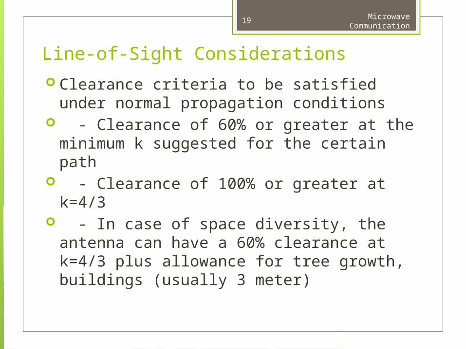
Line-of-Sight Considerations Clearance criteria to be satisfied under normal

propagation conditions - Clearance of 60% or greater at the

minimum k suggested for the certain path - Clearance of 100% or greater at k=4/3 - In case of space diversity, the antenna can

have a 60% clearance at k=4/3 plus allowance for tree growth, buildings (usually 3 meter)

Microwave Communication19

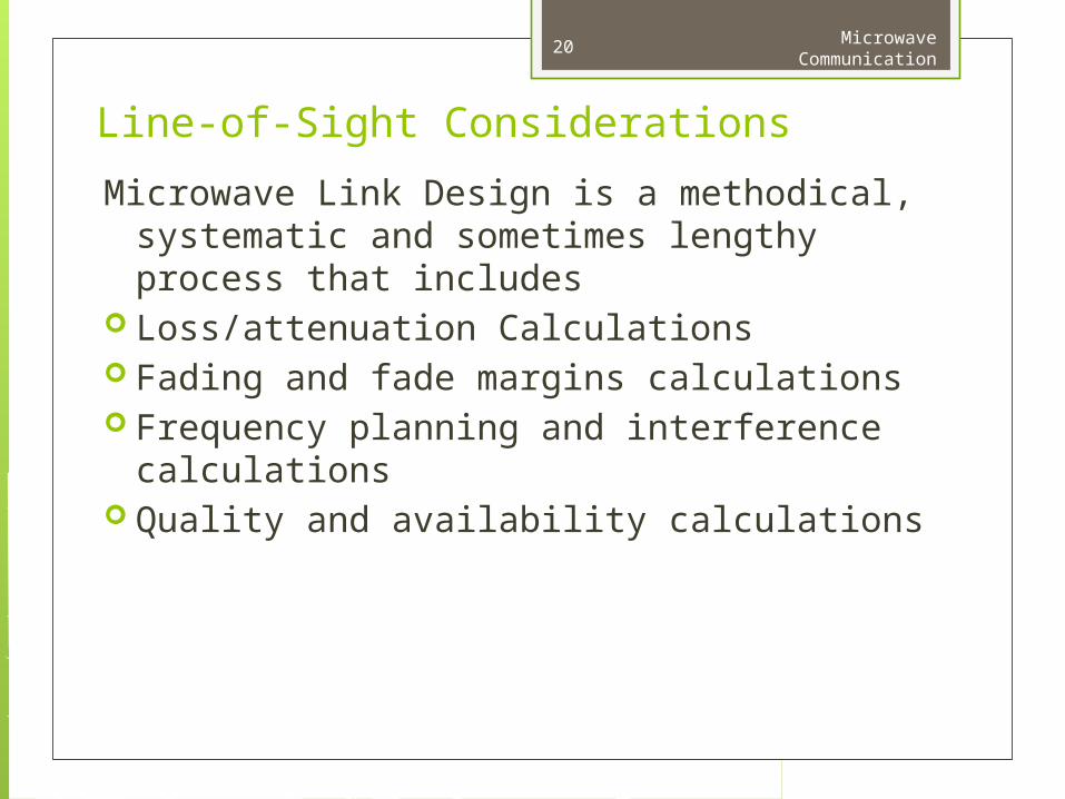
Line-of-Sight Considerations

Microwave Link Design is a methodical, systematic and sometimes lengthy process that includes

Loss/attenuation Calculations Fading and fade margins calculations Frequency planning and interference

calculations Quality and availability calculations

Microwave Communication20

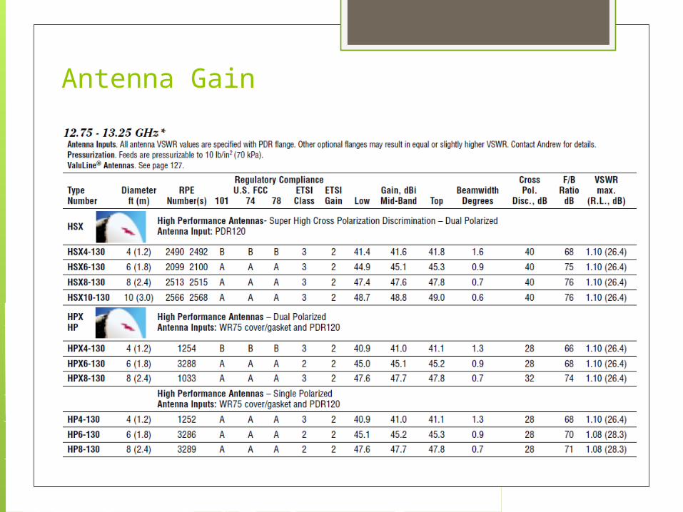
Antenna Gain

2472.10 fDG

2

D

Gwhere: η = Aperture Efficiency(between 0.5 and 0.8) D = Antenna Diameter in meters λ = Wavelength

where: η = Aperture Efficiency(between 0.5 and 0.8) D = Antenna Diameter in meters f = frequency in GHz

fDG log208.17

Antenna Architecture

2 GHz

5 GHz

10.5 GHz

25 GHz0.3 m

0.6 m

1.2 m

3.7m

FIXED GAIN APPROX. 35 dB

Link Analysis FormulasMicrowave Communication

1. Effective Isotropically Radiated Power (EIRP)

the amount of power that would have to be emitted by an isotropic antenna to produce the peak power density observed in the direction of maximum antenna gain.

EIRP = Pt + Gant – TLL

where:

Pt = RF power output (dBm)

Gant = transmit antenna gain (dB)

TLL = total transmission line loss at transmitter (taken from specs, in dB)

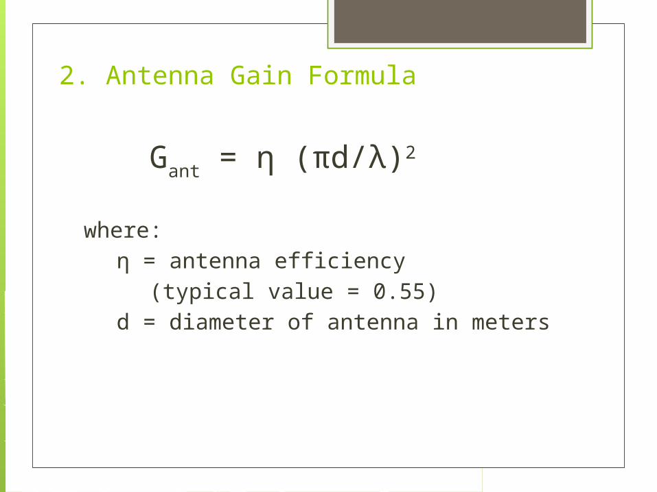
2. Antenna Gain Formula

Gant = η (πd/λ)2

where:η = antenna efficiency

(typical value = 0.55)d = diameter of antenna in meters

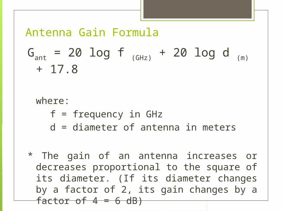
Antenna Gain Formula

Gant = 20 log f (GHz) + 20 log d (m) + 17.8

where:f = frequency in GHzd = diameter of antenna in meters

* The gain of an antenna increases or decreases proportional to the square of its diameter. (If its diameter changes by a factor of 2, its gain changes by a factor of 4 = 6 dB)

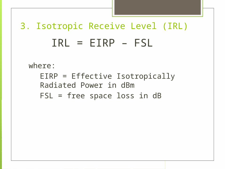
3. Isotropic Receive Level (IRL)

IRL = EIRP – FSL

where:EIRP = Effective Isotropically Radiated Power in dBmFSL = free space loss in dB

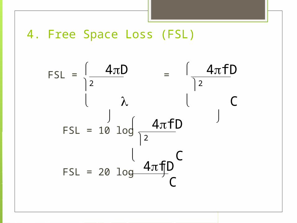
4. Free Space Loss (FSL)

FSL = =

FSL = 10 log

FSL = 20 log

4D 2

4fD 2

C

4fD 2

C

4fD C

Free Space Loss (FSL)

FSL = 20 log (4/C) + 20 log f + 20 log D

When the frequency is given in MHz and distance in km, FSL = 32.4 + 20 log f (MHz) + 20 log D (km)

When the frequency is given in MHz and distance in miles, FSL =36.6 + 20 log f (MHz) + 20 log D (mi)

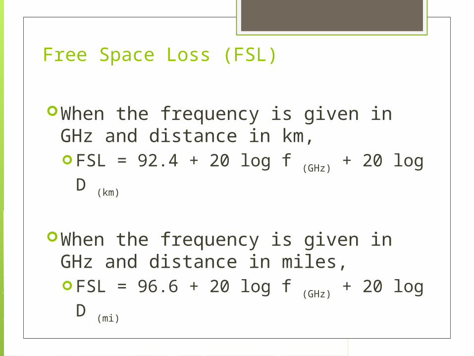
Free Space Loss (FSL)

When the frequency is given in GHz and distance in km, FSL = 92.4 + 20 log f (GHz) + 20 log D (km)

When the frequency is given in GHz and distance in miles, FSL = 96.6 + 20 log f (GHz) + 20 log D (mi)

5. Received Signal Level (RSL) – unfaded

RSL = IRL + Gant – TLL

RSL = Pt + Gant(Tx) – TLL(Tx) – FSL + Gant(Rx) – TLL(Rx)

where:IRL = in dBmGant(Rx) = receive antenna gain (dB)

TLL(Rx) = transmission line loss at receiver

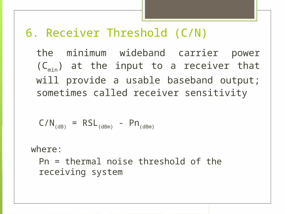
6. Receiver Threshold (C/N)

the minimum wideband carrier power (Cmin) at

the input to a receiver that will provide a usable baseband output; sometimes called receiver sensitivity

C/N(dB) = RSL(dBm) - Pn(dBm)

where:Pn = thermal noise threshold of the

receiving system

7. Thermal Noise Threshold (Pn)

Pn(db) = 174 + 10 log B + NF

where:NF = receiver noise figureB = Bandwidth (hertz)

8. Fade Margin (FM)

equation considers the non-ideal and less predictable characteristics of radio wave propagation such as multi-path loss and terrain sensitivity

Using Barnett-Vignant Equation:

FM = RSL – Receiver Threshold Power Level

FM = 30 log D + 10 log (6ABf) – 10 log (1 –R) – 70

where:30 log D = multi-path effect10 log (6ABf) = terrain sensitivity10 log (1 –R) = reliability objectiveness

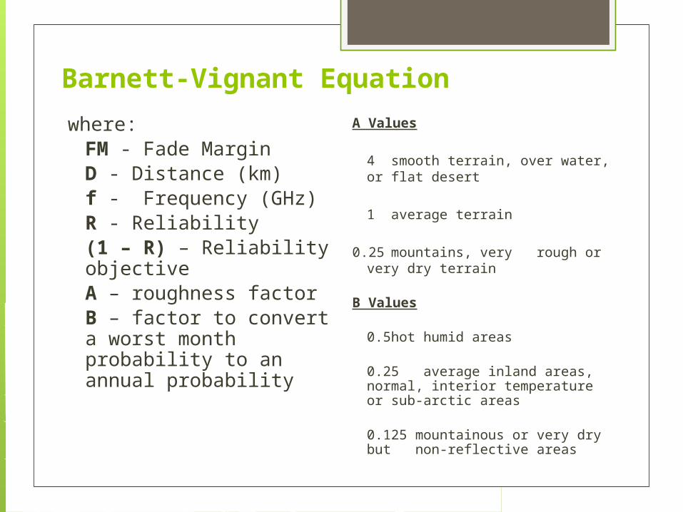
Barnett-Vignant Equation

where:FM - Fade MarginD - Distance (km)f - Frequency (GHz)R - Reliability (1 – R) – Reliability

objectiveA – roughness factorB – factor to convert

a worst month probability to

an annual probability

A Values

4 smooth terrain, over water, or flat desert

1 average terrain

0.25 mountains, very rough or very dry terrain

B Values

0.5 hot humid areas

0.25   average inland areas, normal, interior temperature or sub-arctic areas

0.125 mountainous or very dry but non-reflective areas

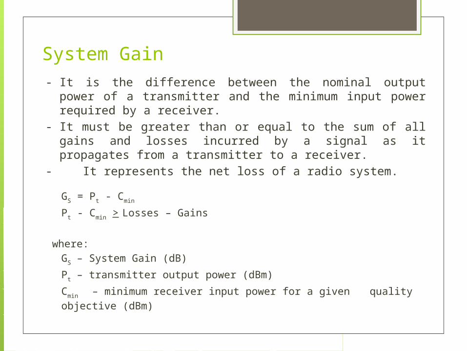
System Gain - It is the difference between the nominal output power of a

transmitter and the minimum input power required by a receiver.

- It must be greater than or equal to the sum of all gains and losses incurred by a signal as it propagates from a transmitter to a receiver.

- It represents the net loss of a radio system.

GS = Pt - Cmin

Pt - Cmin > Losses – Gains

where:GS – System Gain (dB)

Pt – transmitter output power (dBm)

Cmin – minimum receiver input power for a given quality objective (dBm)

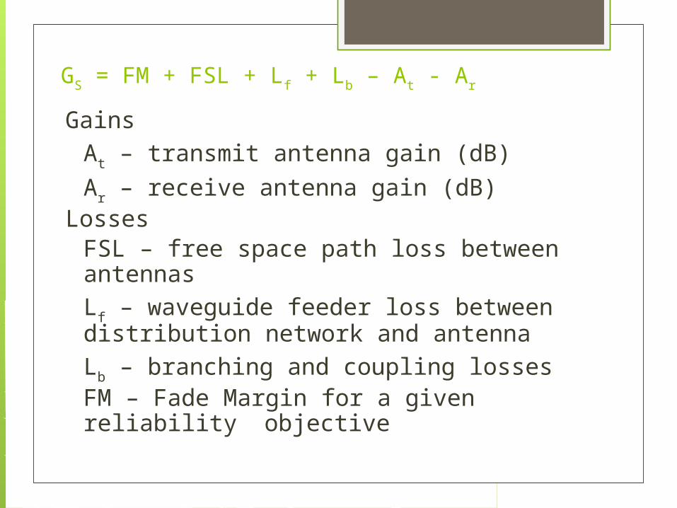
GS = FM + FSL + Lf + Lb – At - Ar

GainsAt – transmit antenna gain (dB)

Ar – receive antenna gain (dB)Losses

FSL – free space path loss between antennasLf – waveguide feeder loss between distribution network and antennaLb – branching and coupling lossesFM – Fade Margin for a given reliability objective

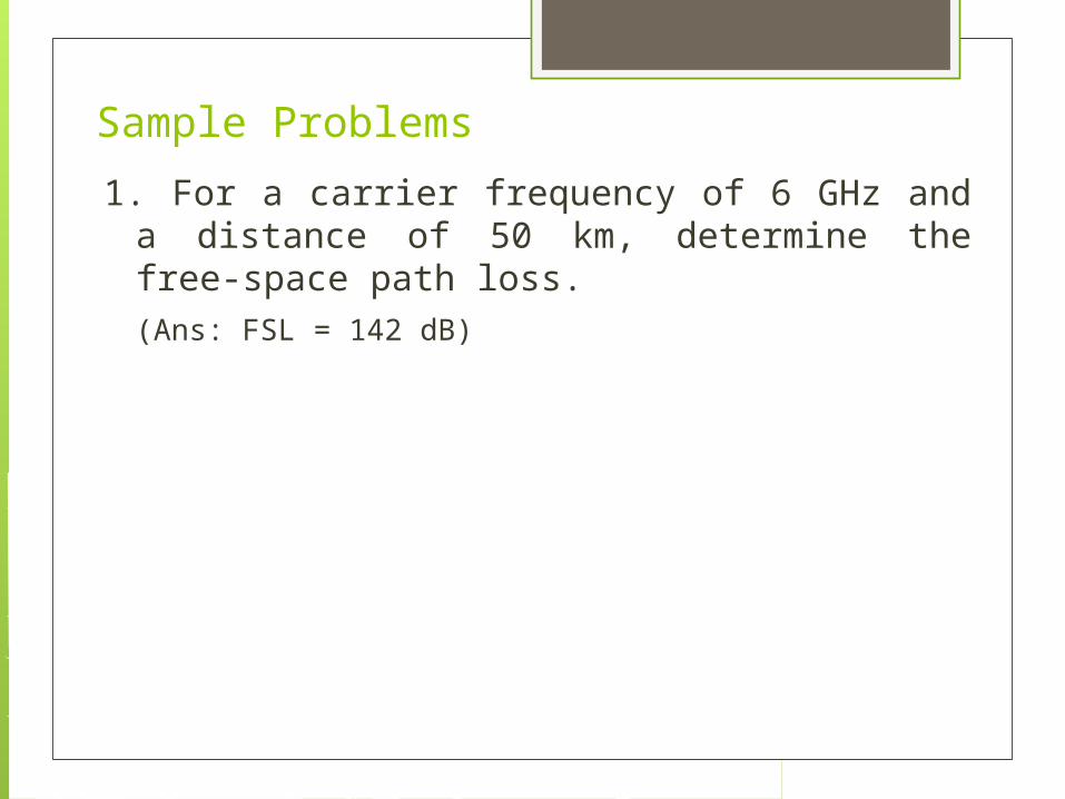
Sample Problems

1. For a carrier frequency of 6 GHz and a distance of 50 km, determine the free-space path loss.(Ans: FSL = 142 dB)

Solution:

Given: f = 6 GHzD = 50 km

Req’d: FSLSol’n:

FSL = 20 log

= 20 log

FSL = 142 dB

4fD C

4(6 x 109)(50 x 103) 3 x 108

2. An FM LOS microwave link operates at 6.15 GHz. The transmitter output power is 1 watt. The path length is 34 km; the antennas at each end have a 35-dB gain and the transmission line losses at each end are 3 dB. Find the received signal level (RSL).(Ans: RSL = -44.85 dBm)

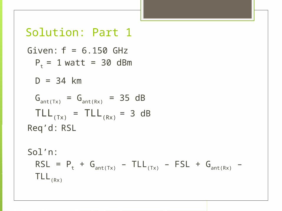
Solution: Part 1

Given: f = 6.150 GHzPt = 1 watt = 30 dBm

D = 34 km

Gant(Tx) = Gant(Rx) = 35 dB

TLL(Tx) = TLL(Rx) = 3 dB

Req’d: RSL

Sol’n:RSL = Pt + Gant(Tx) – TLL(Tx) – FSL + Gant(Rx) – TLL(Rx)

Solution: Part 2

Solving for FSL: FSL = 20 log

= 20 log

FSL = 138. 85 dB

RSL = 30 dBm + 35 dB – 3 dB – 138.85 dB + 35 dB – 3 dB

RSL = - 44.84 dBm

4fD C 4(6.15 x 109)(34 x 103) 3 x 108

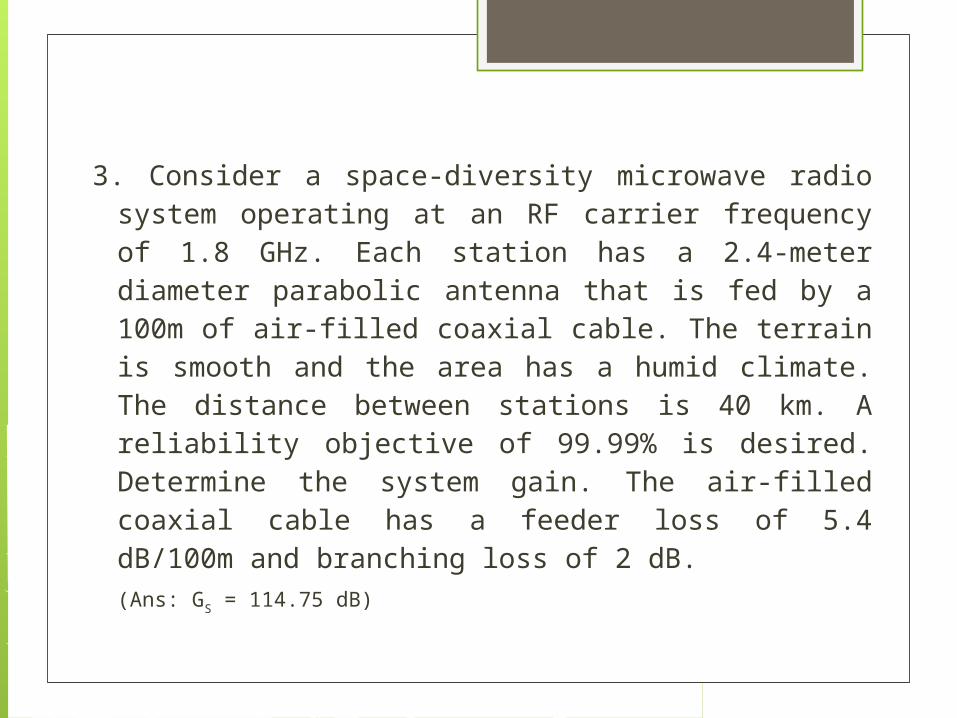
3. Consider a space-diversity microwave radio system operating at an RF carrier frequency of 1.8 GHz. Each station has a 2.4-meter diameter parabolic antenna that is fed by a 100m of air-filled coaxial cable. The terrain is smooth and the area has a humid climate. The distance between stations is 40 km. A reliability objective of 99.99% is desired. Determine the system gain. The air-filled coaxial cable has a feeder loss of 5.4 dB/100m and branching loss of 2 dB.(Ans: GS = 114.75 dB)

Solution: Part 1:

Given: f = 1.8 GHzd = 2.4 m (antenna diameter)

D = 40 kmR = 99.99%Lf = 5.4 dB/100m (each station)

Lb = 2 dB (each station)

Req’d: GS

Sol’n:GS = Pt – Cmin

GS = FM + FSL + Lf + Lb – At - Ar

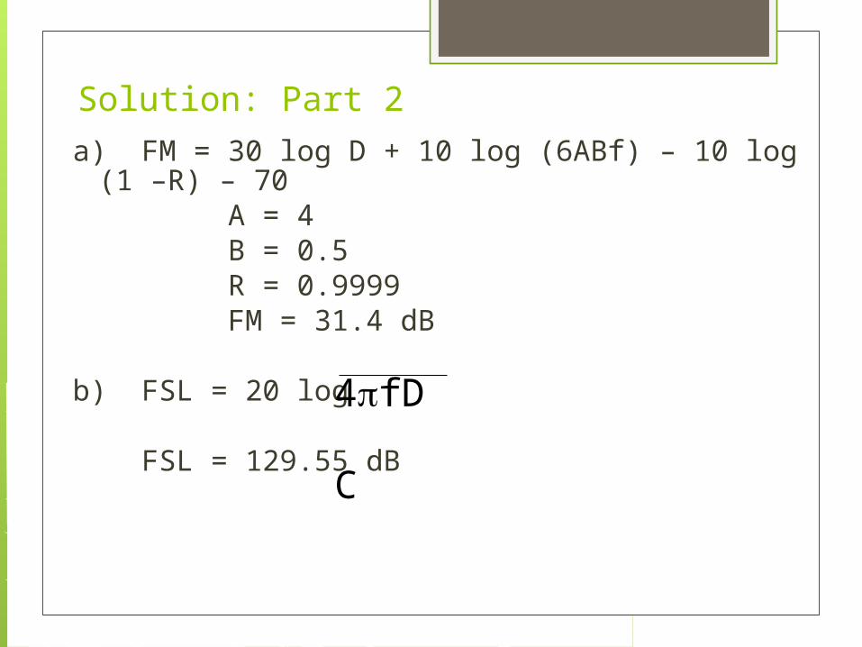
Solution: Part 2a) FM = 30 log D + 10 log (6ABf) – 10 log (1 –

R) – 70A = 4B = 0.5R = 0.9999FM = 31.4 dB

b) FSL = 20 log

FSL = 129.55 dB

4fD C

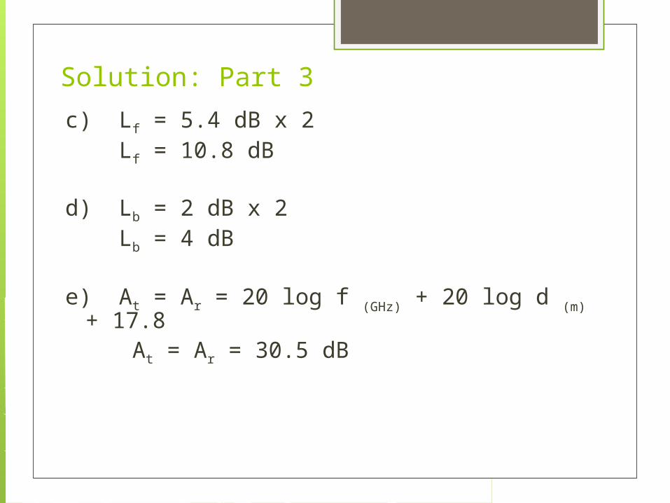
Solution: Part 3

c) Lf = 5.4 dB x 2Lf = 10.8 dB

d) Lb = 2 dB x 2Lb = 4 dB

e) At = Ar = 20 log f (GHz) + 20 log d (m) + 17.8

At = Ar = 30.5 dB

Solution: Part 4

GS = FM + FSL + Lf + Lb – At – Ar

= 31.4 dB + 129.55 dB + 10.8 dB+ 4 dB – 30.5 dB – 30.5 dB

GS = 114.75 dB

* The result indicates that for this system to perform at 99.99% reliability with the given terrain, distribution networks, transmission lines and antennas, the transmitter output power must be at least 114.75 dB more than the minimum receive signal level.

Link BudgetMICROWAVE COMMUNICATION

LINK BUDGET Is basically the summary of all possible

losses and gains that a signal may encounter along a microwave path.

Once the path for a microwave link has been determined, it is necessary to ensure that the received signal power is sufficient for the required signal-to noise ratio.

Transmitter Output Power taken from the data sheet (specifications) of the microwave radio equipment. This is the amount of microwave carrier output power, usually expressed in dBm.

Antenna Gain

Tx Antenna Gain taken from the specifications of the parabolic dish. The amount of increase in the signal density when it

undergoes the process of being focused into a pencil beam.

This amount of gain, usually expressed in dB (over isotropic)

Rx Antenna Gain taken from the specifications of the parabolic dish. This amount of gain, usually expressed in dB (over

isotropic) The amount of increase in the signal density when it

undergoes the process of being focused back into the waveguide.

Antenna Gain

Types of Gain

Received Signal Level (RSL) computed from a formula. This is the amount of input signal into the

receiver from the waveguide. It is the sum of all losses and gains on the

transmitter output.

Receiver Threshold Power taken from specs of radio equipment. This is the minimum amount of microwave

carrier input power, usually expressed in dBm which the receiver can still accurately detect and discriminate information carried. (C/N)

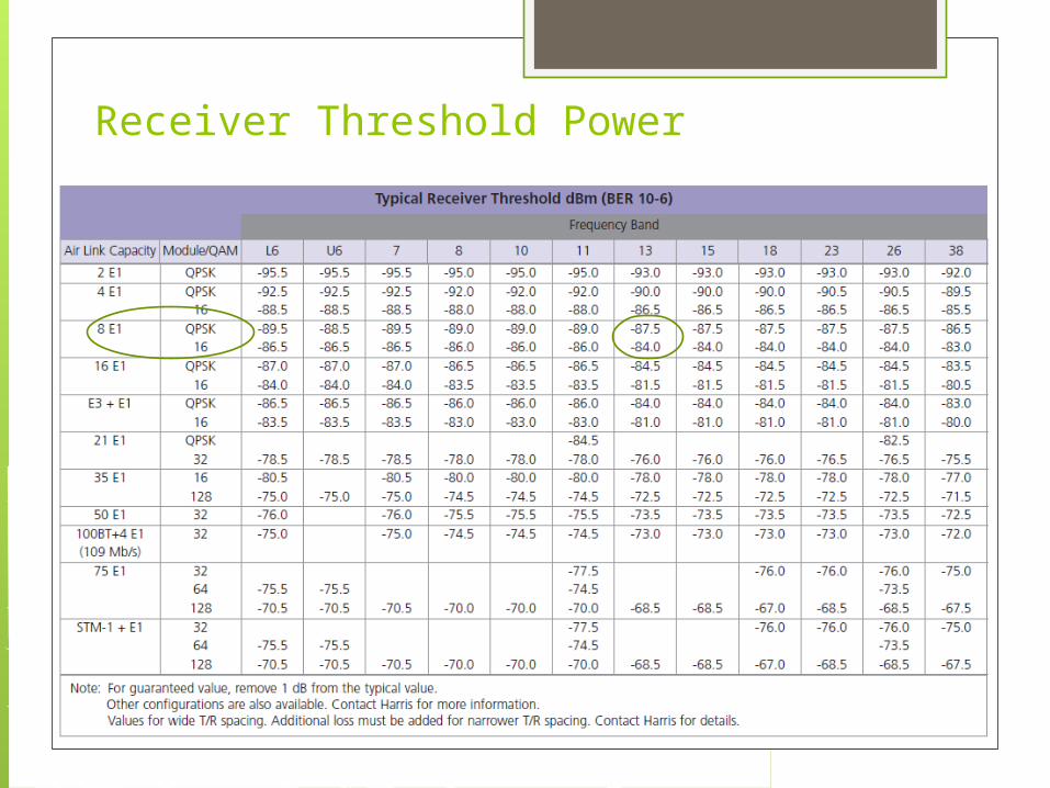
Receiver Threshold Power

Types of LossesLink Budget Analysis

TYPES OF LOSSES

Free Space Loss / Path Attenuation (FSL / PA)

Computed from a formula. This amount of loss, expressed in dB, is how much the signal density reduces as it travels in free space.

Total Transmission Loss losses due to the transmission medium used in

connecting radio equipment to antenna.

Free-Space Loss (FSL)

where D is measured in kilometers;

where D is measured in statute miles;

where D is measured in nautical miles;

MHzkmdB FDFSL log20log2045.32

MHzsmdB FDFSL log20log2058.36

MHznmdB FDFSL log20log2080.37

Note: If F is stated in gigahertz, add 60 to the value of the constant term.

Transmission Losses WAVEGUIDE LOSS

Taken from the specs of the waveguide used. This is the amount of loss, usually expressed in dB per unit length (dB/ft or dB/m) of signal as it travels in the waveguide.

CONNECTOR LOSS taken from specs (0.5 dB)

COUPLING LOSS taken form specs (coax to waveguide to air)

HYBRID LOSS taken from specs, a.k.a circulator loss (1dB)

RADOME LOSS taken from the specs (0.5 dB)

Waveguide Loss

Transmission Losses

CONNECTOR LOSS

COUPLING LOSS

HYBRID LOSS

RADOME LOSS

Fade MarginsParameter Function Value Unit Type Description

Microwave Radio Output Power

Given dB Variable Taken from Radio Specification

Connector Loss Subtracted dB Typical Taken from Waveguide Specifications

Waveguide Loss Subtracted dB Variable Taken from Waveguide Specifications

Connector Loss Subtracted dB Typical Taken from Waveguide Specifications

Antenna Gain Added dB Variable Taken from Antenna Specifications

Free Space Loss Subtracted dB Variable Computed from Formula

Antenna Gain Added dB Variable Taken from Antenna Specifications

Connector Loss Subtracted dB Typical Taken from Waveguide Specifications

Waveguide Loss Subtracted dB Variable Taken from Waveguide Specifications

Connector Loss Subtracted dB Typical Taken from Waveguide Specifications

Power Input to Receiver (RSL)

Computed dB Variable Computed from Formula

Minimum Receiver Threshold

Given dB Variable Taken from Radio Specification

Thermal Fade Margin

Computed dB Variable Computed from Formula

Atmospheric Absorption Loss (AAL)

a. OXYGEN ABSORPTION LOSS- attenuation due to the absorption

of radio frequency energy by oxygen molecules in the atmosphere.

b. WATER VAPOR LOSS- attenuation due to the absorption

of radio frequency energy by water vapor in the atmosphere.

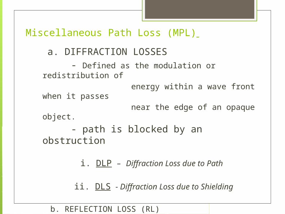
Miscellaneous Path Loss (MPL)

a. DIFFRACTION LOSSES - Defined as the modulation or

redistribution of energy within a wave front when it passes near the edge of an opaque object.

- path is blocked by an obstruction

i. DLP – Diffraction Loss due to Path

ii. DLS - Diffraction Loss due to Shielding

b. REFLECTION LOSS (RL)

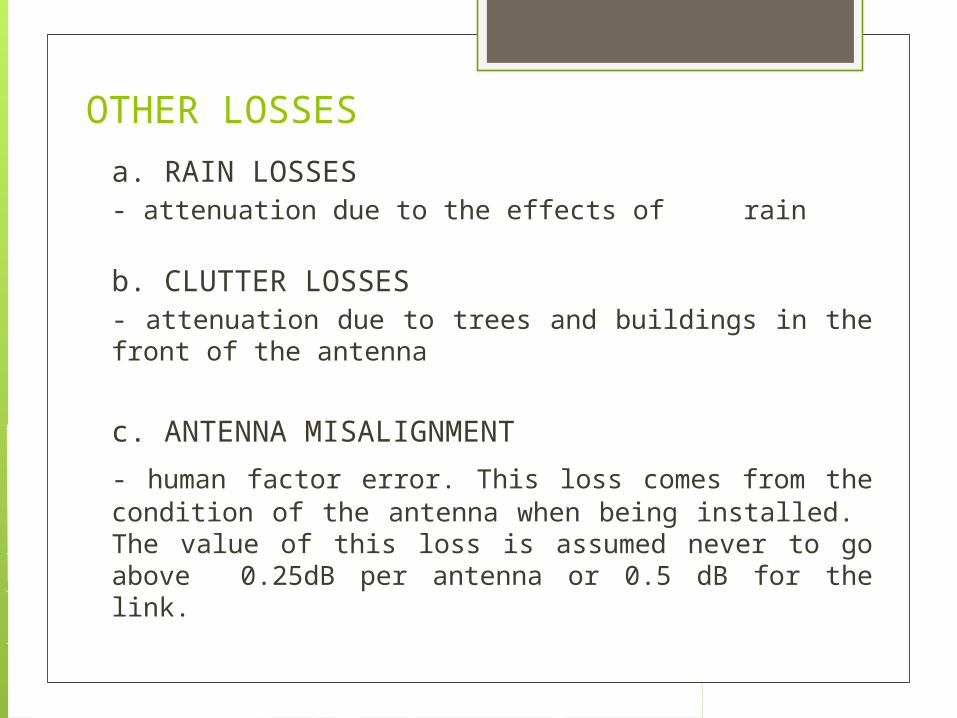
OTHER LOSSES

a. RAIN LOSSES - attenuation due to the effects of rain

b. CLUTTER LOSSES

- attenuation due to trees and buildings in the front of the antenna

c. ANTENNA MISALIGNMENT

- human factor error. This loss comes from the condition of the antenna when being installed. The value of this loss is assumed never to go above 0.25dB per antenna or 0.5 dB for the link.

NET PATH LOSS Difference between the transmitter output

power and the RSL.

Fading and Fade Margin

FadingVariations in signal loss which can be

caused by natural weather disturbances, such as rainfall, snowfall, fog, hail and extremely cold air over a warm earth.

Can also be caused by man-made disturbances, such as irrigation, or from multiple transmission paths, irregular Earth surfaces, and varying terrains.

Fade Margin is the difference between the RSL and the

receiver threshold or sensitivity.

is the additional loss added to the normal path loss to accommodate the effects of temporary fading, that considers the non-ideal and less predictable characteristics of radio-wave propagation

CATEGORIES OF FADING

FLAT FADING non-frequency dependent fading occurring

during atmospheric variations like heavy rain and ducting and aging or partial failure of equipment.

FREQUENCY SELECTIVE FADING due to multipaths formed by atmosphere,

terrain reflection, and diffraction.

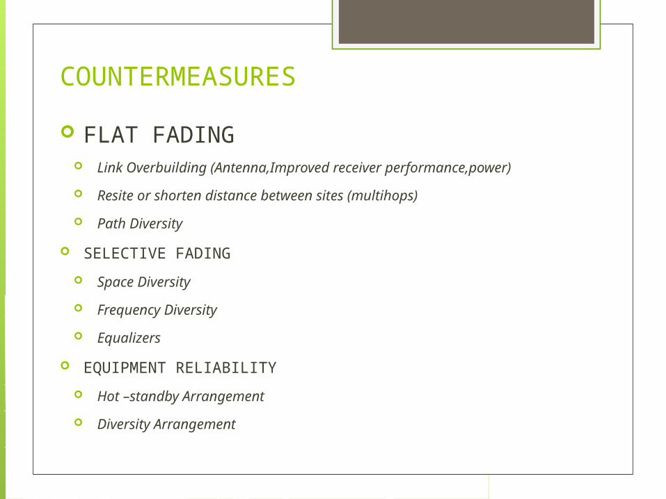
COUNTERMEASURES

FLAT FADING Link Overbuilding (Antenna,Improved receiver performance,power)

Resite or shorten distance between sites (multihops)

Path Diversity

SELECTIVE FADING

Space Diversity

Frequency Diversity

Equalizers

EQUIPMENT RELIABILITY

Hot –standby Arrangement

Diversity Arrangement

Diversity Providing separate path to transmit redundant

information Frequency diversity

Uses two different frequencies to transmit the same information.

Space diversity Same frequency is used, but two receive antennas

separated vertically on the same tower receive the information over two different physical paths separated in space.

The method of transmission may be due to:

a. FREQUENCY

b. SPACE (including angle of arrival and

polarization)

c. PATH (signals arrive on geographically

separate paths)

d. TIME (a time delay of two identical signals

on parallel paths)

PATH DIVERSITY Method of signal rerouting or simultaneous

transmission of same information on different paths. Paths should be at least 10 kms apart.

SPACE DIVERSITY The receiver accepts signals from 2 or

more antennas that are vertically spaced apart by many wavelength (200λ or more)

Depending upon the design, the diversity combiner either selects or adds the signal. If signals are to be added, then they should be brought in phase.

The lower of the two antennas must be high enough for reliable LOS communication.

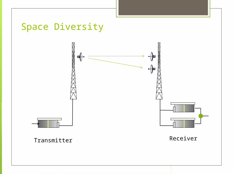
Space Diversity

Transmitter Receiver

Space Diversity Main Features No additional frequency assignment is

required.

Provides path redundancy but not equipment redundancy.

More expensive than frequency diversity due to additional antennas and waveguides.

SPACE DIVERSITY FORMULAAntenna Separation

Formula Improvement Factor

where: S = separation (m)

R = effective earth radius (m)

λ = wavelength (m)

L = path length (m)

Usdp

= Undp lSD

Where: lSD= space diversity improvement factor (Ratio) S = vertical separation bet 2

antennas (m) F = frequency (GHz) D = Path length (m) FM = fade margin, smaller vase (dB)

L

RS

3

D

SfSD

FM10223 101023.1

FREQUENCY DIVERSITY

modulates 2 different RF carrier frequencies with the same IF intelligence, then transmits both RF signals to a given destination.

the carrier frequencies are 2-3% separated, since the frequency band allocations are limited.

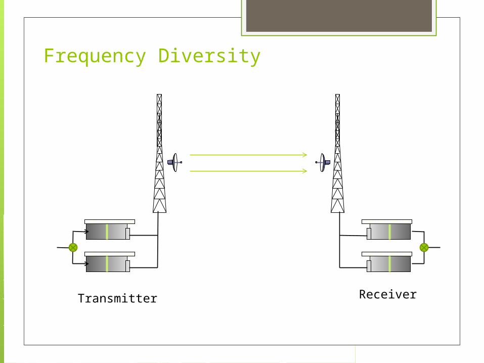
Frequency Diversity

Transmitter Receiver

Improvement Factor of Frequency Diversity

0.8 Dfx 10(FM/10) Undp

lFD = f2D ; UFDP = lFD

Where:

lFD = improvement factor (ratio) Df = Frequency Separation (Mhz)FM = Fade MarginF = frequency (Ghz); (2≤ f ≤ 11)D = Path length (km); (30≤ D ≤ 70)

Time Unavailability Time availability (Av) is commonly in the range

from 0.99 to 0.99999 or 99% to 99.999% of the time.

Unavailability (Unav)is just contrary to the above definition.

vnav AU 1

Fade Margin for Rayleigh Fading

Time Availability (%) Fade Margin (dB)

90 8

99 18

99.9 28

99.99 38

99.999 48

Example:A link with a minimum unfaded C/N specified as 20 dB. What will be the C/N requirements to meet the objective of 99.95% time availability? What is the total time in a year when the C/N would be less than 20 dB?

References Radio System Design for Telecommunication,

Third Edition Roger L. Freeman Copyright © 2007 John Wiley & Sons, Inc.

Microwave Transmission Networks Harvey Lehpamer Copyright © 2004 McGraw-Hill Companies, Inc.

Fundamentals of Microwave Communication Manny T. Rule

Microwave Engineering Design Consideration Lenkurt

THANK YOU…