2

Dedication

To my wife and my children Reem and Mohab,

and

my company ANSDK

ACKNOWLEDGEMENT

I would like to express my deep thanks to my supervisor Dr Syed Hassan for his great

support and guidance throughout the project. I would like also to thank Dr Rachel

Clington for her assistance especially with the preparation of the machine for the test.

I am also grateful to Mr. Wilknson, the technical manager of the school, for his always

support. I’d like to express my thanks to Brain (workshop) for his efforts to solve the

problems I had with the creep-testing machine.

3

Table of Contents

Preface 5

1. Introduction 6

2. Characteristics of High Temperature Applications 10

3. Creep Curve 13

4. Creep Characteristics

4.1 Time 17

4.2 Temperature 17

4.3 Stress 18

4.4 Microstructure 18

5. Fundamentals Mechanisms Responsible for Creep 19

5.1 Diffusion Creep Process 21

5.1.1 Lattice Diffusion Creep 24

5.1.2 Grain Boundary Diffusion Creep 26

5.2 Dislocation Creep 28

5.3 Grain Boundary Sliding and Supperplasticity 30

6. Micro-Mechanical Deformation Mechanisms During Creep 33

6.1 Intragranular Creep Deformation

6.1.1 Crystallographic Slip 33

6.1.2 Sub grain Formation 34

6.2 Intergranular Creep Deformation

6.2.1 Grain Boundary Sliding 35

6.2.2 Creep Cavity Nucleation 36

6.2.3 Fold Formation and Grain Boundary Migration 37

7. Creep Life Assessment

7.1 Current Approaches of Creep Life Assessment 39

7.1.a Operational Condition Monitoring Approach 40

7.1.b Methods Based on Post-Service Examination Sampling and

Calculation 40

7.1.1 Creep Rupture Testing 41

7.1.1.1 Larson Miller Method 41

4

7.1.1.2 Manson and Hafered Method 42

7.1.1.3 Orr-Shery-Dorn Method 43

7.1.2 Strain Measurement Methods 44

7.2 Mechanistic Models of Creep Damage Process

7.2.1 Reduction in Load Bearing Section 44

7.2.2 Micro structural Degradation 45

7.2.3 Cavitation Damage 45

7.2.4 Effect of Environment 46

7.3 Phenomenological Models 46

8. Material Specifications

8.1 Chemical Composition 49

8.2 Mechanical Properties at Room Temperature 49

8.3 Physical Properties 50

9. Experimental Procedures

9.1 Test Pieces 51

9.2 Impact Test 52

9.3 Hardness Test 54

9.4 Tensile Test 56

9.5 Accelerated Creep Rupture Test 58

9.5.1 Test Technique 58

9.5.2 Test Procedure 59

9.6 Microstructure Examination 75

10. Analysis of The Tests Result 78

11. Conclusion 85

12. Future Plan and Recommendation 86

13. References

14. Appendixes

14.1 List of Figures 89

14.2 List of Tables 93

14.3 Recorded Test Results 94

5

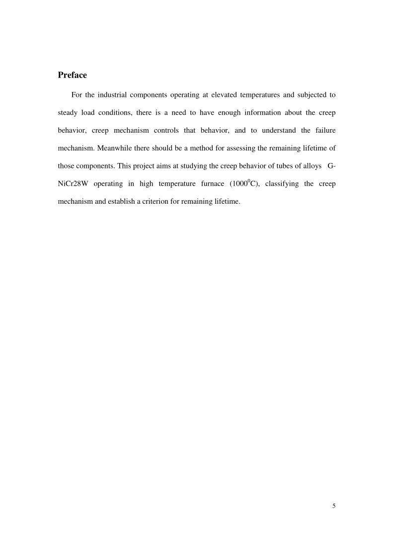
Preface

For the industrial components operating at elevated temperatures and subjected to

steady load conditions, there is a need to have enough information about the creep

behavior, creep mechanism controls that behavior, and to understand the failure

mechanism. Meanwhile there should be a method for assessing the remaining lifetime of

those components. This project aims at studying the creep behavior of tubes of alloys G-

NiCr28W operating in high temperature furnace (10000C), classifying the creep

mechanism and establish a criterion for remaining lifetime.

6

1. Introduction

Alexandria National Iron and Steel Co. (ANSDK) is one of the leading companies in

the Middle East for producing reinforced steel. The company consists of four main plants

• Direct reduction plant,

• Steel making plant,

• Continuous casting plant, and

• Rolling plant.

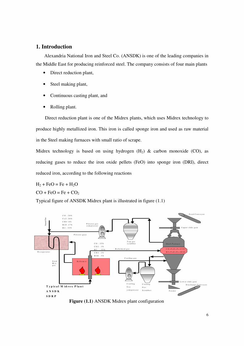
Direct reduction plant is one of the Midrex plants, which uses Midrex technology to

produce highly metallized iron. This iron is called sponge iron and used as raw material

in the Steel making furnaces with small ratio of scrape.

Midrex technology is based on using hydrogen (H2) & carbon monoxide (CO), as

reducing gases to reduce the iron oxide pellets (FeO) into sponge iron (DRI), direct

reduced iron, according to the following reactions

H2 + FeO = Fe + H2O

CO + FeO = Fe + CO2

Typical figure of ANSDK Midrex plant is illustrated in figure (1.1)

Nat

ura

l G

as

C O : 2 0 %

C o 2 : 2 0 %

C H 4 : 8 %

H 2 0 : 1 7 %

H 2 : 3 5 %

R e c u p e r a t o r

R e f o r m e r

C O : 3 5 %

C O 2 : 3 %

H 2 : 5 5 %

C H 4 : 2 %

H 2 O : 5 %

C o o l i n g

G a s

S c r u b b e r

C o o l i n g

G a s

c o m p r e s s o r

T o p g a s

s c r u b b e r

P r o c e s s g a s

c o m p r e s s o r

S h a f t F u r n a c e

T y p i c a l M i d r e x P l a n t

A N S D K

S D R P

R e f o r m e d g a s

P r o c e s s g a a s

C o o l i n g g a s

C O + F e O = F e + C O 2

H 2 + F e O = F e + H 2 O

F e e d C o n v e y o r

D i s c h a r g e C o n v e y o r

F e e d e r

U p p e r s l i d e g a t e

L o w e r s l i d e g a t e

F e e d

M i x

g a s

Figure (1.1) ANSDK Midrex plant configuration

7

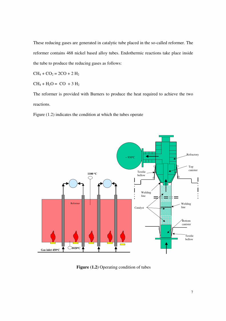
These reducing gases are generated in catalytic tube placed in the so-called reformer. The

reformer contains 468 nickel based alloy tubes. Endothermic reactions take place inside

the tube to produce the reducing gases as follows:

CH4 + CO2 = 2CO + 2 H2

CH4 + H2O = CO + 3 H2

The reformer is provided with Burners to produce the heat required to achieve the two

reactions.

Figure (1.2) indicates the condition at which the tubes operate

Reformer

1100 oC

1020oCGas inlet 450oC

Catalyst

~ 930oC

Welding

line

Welding

line

Refractory

Top

canister

Bottom

canister

Textile

bellow

Textile

bellow

Figure (1.2) Operating condition of tubes

8

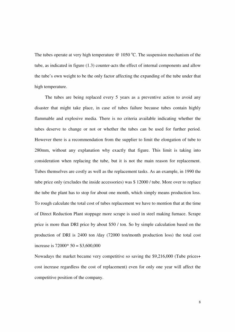
The tubes operate at very high temperature @ 1050 oC. The suspension mechanism of the

tube, as indicated in figure (1.3) counter-acts the effect of internal components and allow

the tube’s own weight to be the only factor affecting the expanding of the tube under that

high temperature.

The tubes are being replaced every 5 years as a preventive action to avoid any

disaster that might take place, in case of tubes failure because tubes contain highly

flammable and explosive media. There is no criteria available indicating whether the

tubes deserve to change or not or whether the tubes can be used for further period.

However there is a recommendation from the supplier to limit the elongation of tube to

280mm, without any explanation why exactly that figure. This limit is taking into

consideration when replacing the tube, but it is not the main reason for replacement.

Tubes themselves are costly as well as the replacement tasks. As an example, in 1990 the

tube price only (excludes the inside accessories) was $ 12000 / tube. More over to replace

the tube the plant has to stop for about one month, which simply means production loss.

To rough calculate the total cost of tubes replacement we have to mention that at the time

of Direct Reduction Plant stoppage more scrape is used in steel making furnace. Scrape

price is more than DRI price by about $50 / ton. So by simple calculation based on the

production of DRI is 2400 ton /day (72000 ton/month production loss) the total cost

increase is 72000* 50 = $3,600,000

Nowadays the market became very competitive so saving the $9,216,000 (Tube prices+

cost increase regardless the cost of replacement) even for only one year will affect the

competitive position of the company.

9

This study aims at investigating the creep behavior of the tube under the used

temperatures and its own weight. This investigation will be through conducting

accelerated creep rupture. Establishing of criteria for tubes replacement will be obtaining

from the resulted creep behavior curve from the test. The purpose of this is to save money

spending without actually need for that spending and consequently increasing the

profitability of the company and strengthened its competitive position. In addition to that

other tests such as tensile test impact test, hardness test will also be conducted to have

some properties of the tube alloy at room and elevated temperatures.

Counter weight~600 Kg

Tension

W ire

Suspension mechanism

Reformer structure

Pulley

Figure (1.3) Suspension mechanism of tube

10

2. Characteristics of High Temperature Applications

The technological developments since the early 20th century has required materials

that resist very high temperatures. Applications of these developments lie mainly in the

following areas:1

1. Gas turbine (stationary and on craft), whose blades operate at temperatures

of 800- 900 K. The burner and after burner sections operate at higher

temperatures, 1300 – 1400 K.

2. Nuclear reactors where pressure vessels and piping operate at 560 – 750 K.

Reactor skirts operate at 850- 950 K.

3. Chemical and petrochemical industries where some steam reformers

operate at 1250- 1350 K.

Materials used in these applications are subjected to a working temperatures

range (0.4~0.65) Tm, where Tm is the melting point of the material. Of course these

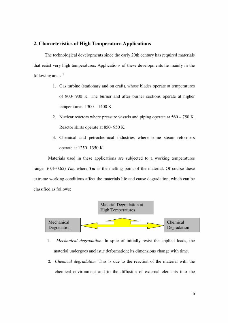
extreme working conditions affect the materials life and cause degradation, which can be

classified as follows:

1. Mechanical degradation. In spite of initially resist the applied loads, the

material undergoes anelastic deformation; its dimensions change with time.

2. Chemical degradation. This is due to the reaction of the material with the

chemical environment and to the diffusion of external elements into the

Mechanical Degradation

Chemical Degradation

Material Degradation at High Temperatures

11

materials. Chlorination (which affects the properties of super alloys used in

jet turbines) and internal oxidation are examples of chemical degradation.

Our concern here is the mechanical degradation. The thermo-mechanical

degradation or time dependant deformation of a material is known as creep.

Micro-structural changes take place at elevated temperatures; lead to materials failure at a

stress that is much lower than its ultimate tensile strength measured at ambient

temperature. A great number of failures can be attributed either to creep or to a

combination of creep and fatigue. Creep is characterized by a slow flow of the material,

which behaves as if it were viscous. If a component of a structure is subjected to a

constant tensile load, the decrease in cross-sectional area (due to the increase in length

resulting from creep) generates an increase in stress; when the stress reaches the value at

which failure occurs statically (ultimate tensile stress), failure occurs. Elastic, plastic,

visco-elastic, and visco-plastic deformations can all be included in the creep process,

depending on the material and the characteristic time of the deformation. However, creep

deformation is always treated as plastic deformation because the failures associated with

creep are similar to those due to yield in plastic deformation of the materials. There are

various mechanisms of creep in materials at elevated temperatures and thus there are

different creep models.

The temperature range, in Kelvin, for which creep is important in metals and

ceramics, is 0.4 Tm <T<Tm, where Tm is the melting temperature of the material and T is

the operating temperature.

The critical temperature for creep varies from material to another; lead material

creeps at ambient temperature, whereas creep becomes important in iron above 6000C. In

12

general, the phenomenon of creep is important at high temperatures. Some nickel-based

super alloys can withstand temperatures as high as 1,500 K, and ceramics have

temperature capabilities that are considerably higher (up to 2,000 K).1

13

3. Creep curve

A creep curve measures the resistance of the material to time dependence

deformation under load. When a constant load is applied to a tensile specimen at a

constant temperature (usually greater than 0.4 ~0.5 of the absolute melting temperature of

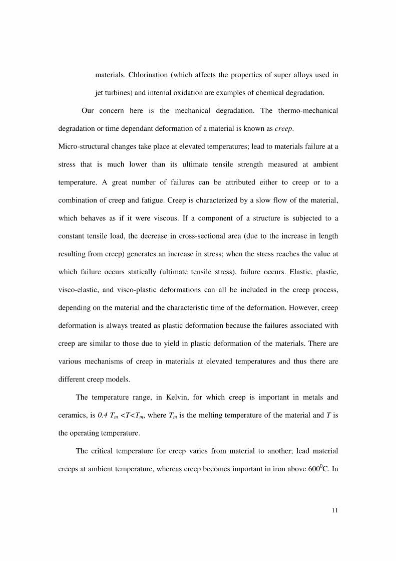
the specimen) the strain of the specimen is determined as a function of time. A typical

variation of creep strain with time in a specimen is shown in figure (3.1). The slope of

this curve is the creep rate.3

Creep is characterized as having three distinct stages,

Stage 1 of curve (A), which represents the creep test at constant load, follows after an

initial instantaneous strain �o, which includes both elastic and plastic deformations. This

stage is termed as primary stage within which the creep rate decreases with time.

Stage 2 or secondary creep stage during this stage the creep rate approaches stable

minimum value and relatively constant over the time. Creep rate is termed as steady state

Figure (3.1) Typical Creep Curve Showing the 3 Stages of Creep. Reference IEEE Transaction on Reliability Vol.42, NO.3, 1993

14

creep rate. It is also known as the minimum creep rate, because it corresponds to the

inflection point of the curve. The steady state creep rate is an important engineering

property, because most deformations involve this stage.

Stage 3 termed as tertiary creep, in which the creep rate accelerates with time and leads

to failure by creep rupture.

Although the three stages represent the creep behavior in most materials, the primary

creep stage can be absent for some materials. The extension during the tertiary creep

stage can be limited in brittle materials and very extensive in ductile materials.

Curve (B) in figure is different from curve (A) and indicates a creep test with a constant

stress.

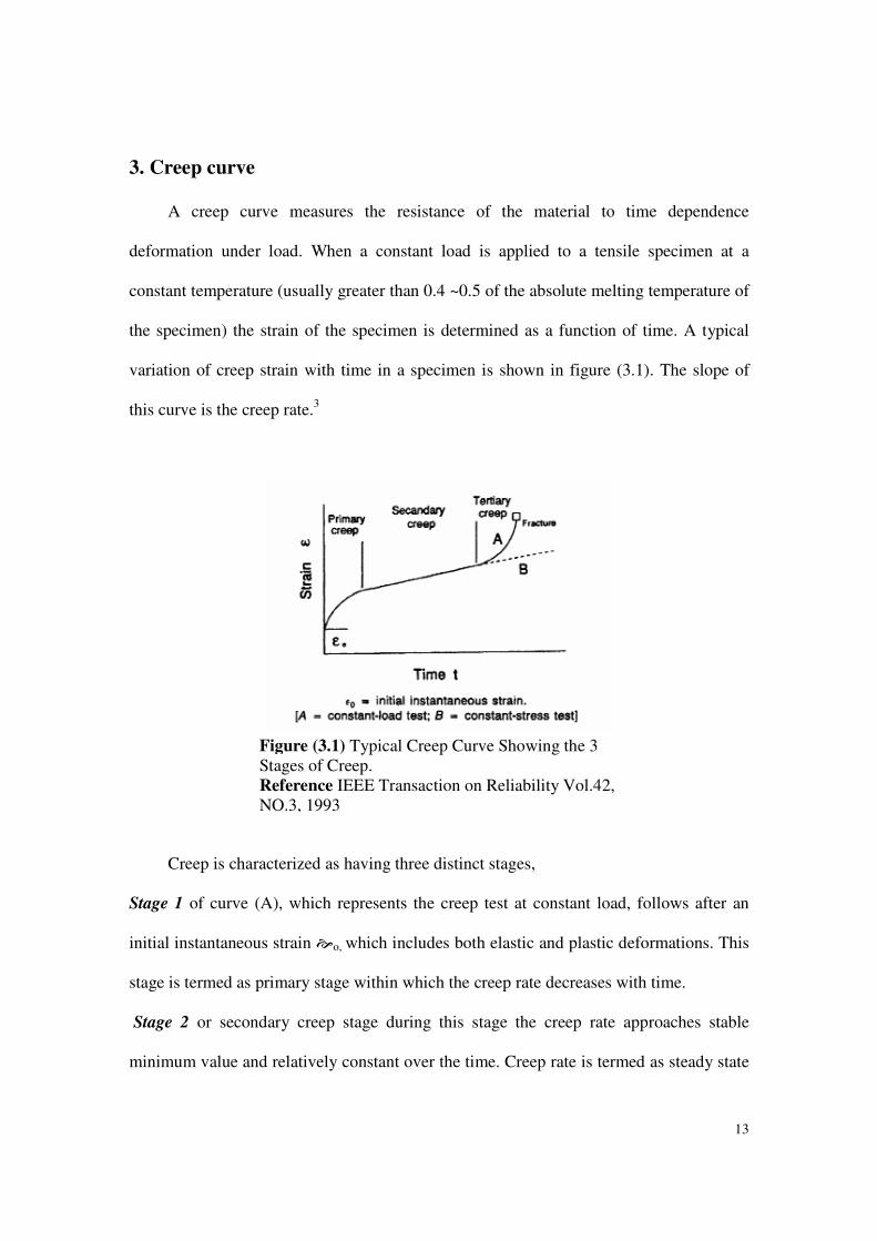
The creep test is rather simple and consists of subjecting a specimen to a constant

load (or stress) and measuring its length as a function of time, at a constant temperature.

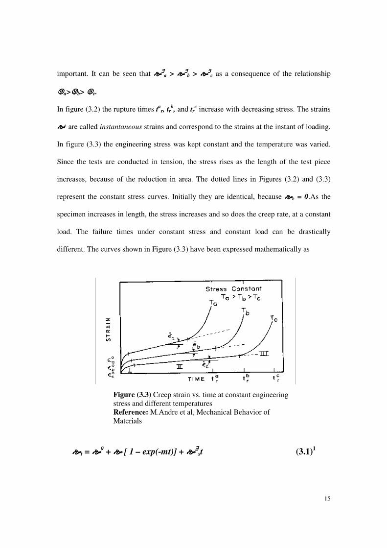
Figure (3.2) shows the characteristic curve under different stresses; the ordinate shows

the strain and the abscissa shows time. Three tests are represented in the figure; three

constant loads corresponding to three engineering stresses, 9a, 9b, and 9c, were used.

Stage II, as mentioned above, in which the creep rate �∃∃∃∃ is constant, is the most

Figure (3.2) Creep strain vs. time at difference constant

stress levels and temperatures

15

important. It can be seen that ��∃∃∃∃

a > ��∃∃∃∃

b > ��∃∃∃∃

c as a consequence of the relationship

9999a>9999b> 9999c.

In figure (3.2) the rupture times tar, tr

b, and tr

c increase with decreasing stress. The strains

��0 are called instantaneous strains and correspond to the strains at the instant of loading.

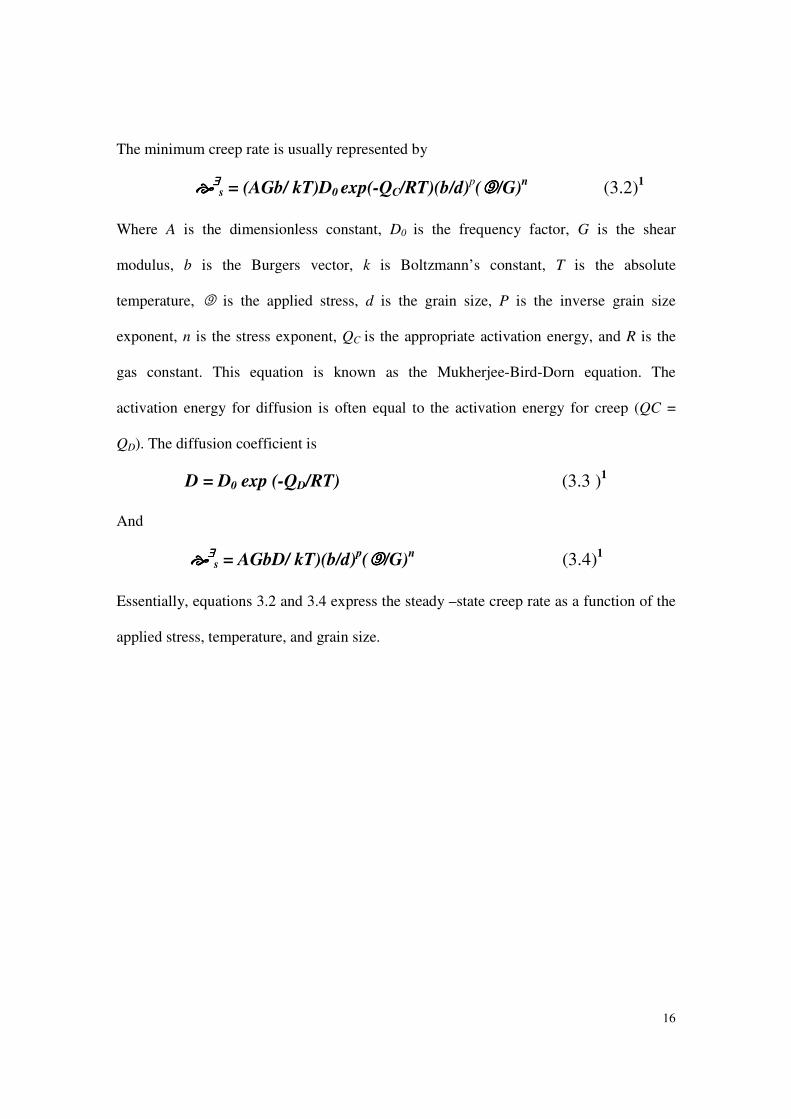
In figure (3.3) the engineering stress was kept constant and the temperature was varied.

Since the tests are conducted in tension, the stress rises as the length of the test piece

increases, because of the reduction in area. The dotted lines in Figures (3.2) and (3.3)

represent the constant stress curves. Initially they are identical, because ��e = 0.As the

specimen increases in length, the stress increases and so does the creep rate, at a constant

load. The failure times under constant stress and constant load can be drastically

different. The curves shown in Figure (3.3) have been expressed mathematically as

��t = ��0 + �� [ 1 – exp(-mt)] + ��

∃∃∃∃st (3.1)

1

Figure (3.3) Creep strain vs. time at constant engineering stress and different temperatures Reference: M.Andre et al, Mechanical Behavior of Materials

16

The minimum creep rate is usually represented by

��∃∃∃∃

s = (AGb/ kT)D0 exp(-QC/RT)(b/d)p(9999/G)

n (3.2)1

Where A is the dimensionless constant, D0 is the frequency factor, G is the shear

modulus, b is the Burgers vector, k is Boltzmann’s constant, T is the absolute

temperature, 9 is the applied stress, d is the grain size, P is the inverse grain size

exponent, n is the stress exponent, QC is the appropriate activation energy, and R is the

gas constant. This equation is known as the Mukherjee-Bird-Dorn equation. The

activation energy for diffusion is often equal to the activation energy for creep (QC =

QD). The diffusion coefficient is

D = D0 exp (-QD/RT) (3.3 )1

And

��∃∃∃∃

s = AGbD/ kT)(b/d)p(9999/G)

n (3.4)1

Essentially, equations 3.2 and 3.4 express the steady –state creep rate as a function of the

applied stress, temperature, and grain size.

17

4. Creep Characteristics

Creep characteristics depend on several factors such as time, temperature, Stress, and the

microstructure.

4.1 Time.

A time scale is always involved in a creep test. As a comparison, for most

engineering materials tested at low temperatures, measured tensile properties are

relatively dependent of the test time, regardless of whether it is 5 minutes or 5 hour. The

main reason of that is the involvement of the thermally activated time dependent

processes. A single dominant thermally activated process usually controls the overall

creep rate during creep deformation. For example, if the controlling process is

diffusional, the creep rate is called diffusion controlled.1

4.2 Temperature

Normally the creep processes involve mechanisms at the atomic scale. The mobility

of atoms and vacancies increases rapidly with temperature so they can diffuse through the

lattice of the material along the direction of the hydrostatic stress gradient, which is

called self-diffusion. The self-diffusion of atoms can or vacancies helps dislocations (line

crystal defect) climb (a motion of dislocation toward the direction perpendicular to its

slip plane). At low temperatures, becomes less diffusion- controlled. Diffusion can occur,

but is limited in local porous areas, like grain boundaries and phase interfaces, which is

called grin boundary diffusion.3 Generally creep becomes of engineering importance at

T>0.5Tm. This is just empirical guideline based on the observations that above 0.5 Tm,

creep is most likely to be governed by mechanisms that depend on self-diffusion.

18

4.3 Stress

Stress level and stress state greatly affect the creep rate. As explained in figure (3.2)

shows the effect of different stress at constant temperature.

Measurements of creep property are classified into creep test and creep rupture test

according to the stress level.

• Creep test

Normally the test is carried out at low stresses to determine the steady state creep

rate. The total strain is often less than 0.5%

• Creep rupture test

It is similar to creep test except that high load is applied to precipitate failure of

the material. The total strain can be as high as 50%.

4.4 Micro-structure

Microstructure of the material plays an important part of determining the creep

behavior of the material. Grain size affects the creep rate in all the three stages.

Precipitations and impurity particles initiate creep cavities. Porosity due to sintering,

particularly in ceramics, is another microstructure effect.10

19

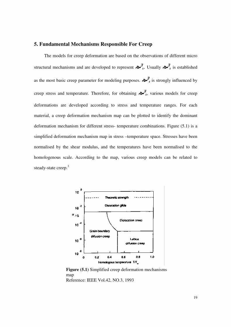
5. Fundamental Mechanisms Responsible For Creep

The models for creep deformation are based on the observations of different micro

structural mechanisms and are developed to represent ��∃∃∃∃

s. Usually ��∃∃∃∃

s is established

as the most basic creep parameter for modeling purposes. ��∃∃∃∃

s is strongly influenced by

creep stress and temperature. Therefore, for obtaining ��∃∃∃∃

s, various models for creep

deformations are developed according to stress and temperature ranges. For each

material, a creep deformation mechanism map can be plotted to identify the dominant

deformation mechanism for different stress- temperature combinations. Figure (5.1) is a

simplified deformation mechanism map in stress –temperature space. Stresses have been

normalised by the shear modulus, and the temperatures have been normalised to the

homologenous scale. According to the map, various creep models can be related to

steady-state creep.3

Figure (5.1) Simplified creep deformation mechanisms map Reference: IEEE Vol.42, NO.3, 1993

20

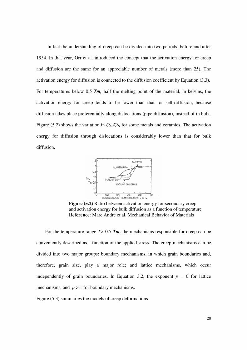
In fact the understanding of creep can be divided into two periods: before and after

1954. In that year, Orr et al. introduced the concept that the activation energy for creep

and diffusion are the same for an appreciable number of metals (more than 25). The

activation energy for diffusion is connected to the diffusion coefficient by Equation (3.3).

For temperatures below 0.5 Tm, half the melting point of the material, in kelvins, the

activation energy for creep tends to be lower than that for self-diffusion, because

diffusion takes place preferentially along dislocations (pipe diffusion), instead of in bulk.

Figure (5.2) shows the variation in QC /QD for some metals and ceramics. The activation

energy for diffusion through dislocations is considerably lower than that for bulk

diffusion.

For the temperature range T> 0.5 Tm, the mechanisms responsible for creep can be

conveniently described as a function of the applied stress. The creep mechanisms can be

divided into two major groups: boundary mechanisms, in which grain boundaries and,

therefore, grain size, play a major role; and lattice mechanisms, which occur

independently of grain boundaries. In Equation 3.2, the exponent p = 0 for lattice

mechanisms, and p > 1 for boundary mechanisms.

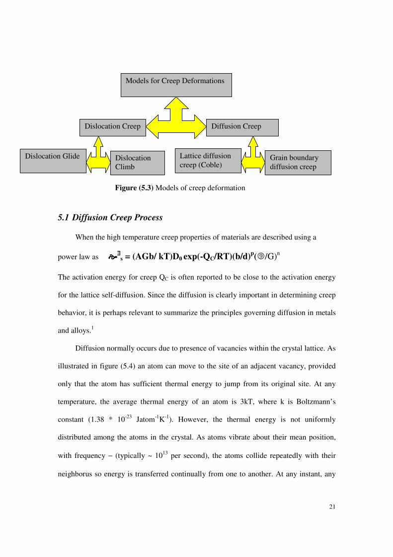
Figure (5.3) summaries the models of creep deformations

Figure (5.2) Ratio between activation energy for secondary creep and activation energy for bulk diffusion as a function of temperature

Reference: Marc Andre et al, Mechanical Behavior of Materials

21

5.1 Diffusion Creep Process

When the high temperature creep properties of materials are described using a

power law as ��∃∃∃∃

s = (AGb/ kT)D0 exp(-QC/RT)(b/d)p(9/G)n

The activation energy for creep QC is often reported to be close to the activation energy

for the lattice self-diffusion. Since the diffusion is clearly important in determining creep

behavior, it is perhaps relevant to summarize the principles governing diffusion in metals

and alloys.1

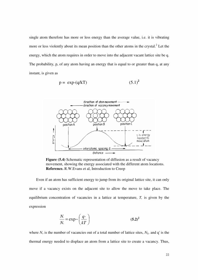
Diffusion normally occurs due to presence of vacancies within the crystal lattice. As

illustrated in figure (5.4) an atom can move to the site of an adjacent vacancy, provided

only that the atom has sufficient thermal energy to jump from its original site. At any

temperature, the average thermal energy of an atom is 3kT, where k is Boltzmann’s

constant (1.38 * 10-23 Jatom-1K-1). However, the thermal energy is not uniformly

distributed among the atoms in the crystal. As atoms vibrate about their mean position,

with frequency − (typically ~ 1013 per second), the atoms collide repeatedly with their

neighborus so energy is transferred continually from one to another. At any instant, any

Models for Creep Deformations

Diffusion Creep

Dislocation Creep

Lattice diffusion creep (Coble)

Dislocation Glide

Figure (5.3) Models of creep deformation

Grain boundary diffusion creep

Dislocation Climb

22

single atom therefore has more or less energy than the average value, i.e. it is vibrating

more or less violently about its mean position than the other atoms in the crystal.2 Let the

energy, which the atom requires in order to move into the adjacent vacant lattice site be q.

The probability, p, of any atom having an energy that is equal to or greater than q, at any

instant, is given as

p = exp-(q/kT) (5.1)2

Even if an atom has sufficient energy to jump from its original lattice site, it can only

move if a vacancy exists on the adjacent site to allow the move to take place. The

equilibrium concentration of vacancies in a lattice at temperature, T, is given by the

expression

−=

kT

q

N

N

L

v ^

exp (5.2)2

where Nv is the number of vacancies out of a total number of lattice sites, NL, and q' is the

thermal energy needed to displace an atom from a lattice site to create a vacancy. Thus,

Figure (5.4) Schematic representation of diffusion as a result of vacancy movement, showing the energy associated with the different atom locations.

Reference. R.W.Evans et al, Introduction to Creep

23

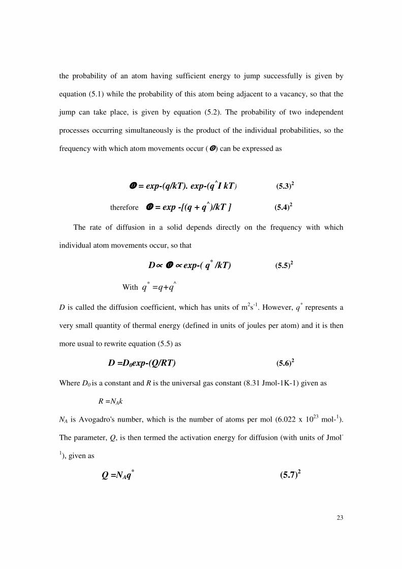
the probability of an atom having sufficient energy to jump successfully is given by

equation (5.1) while the probability of this atom being adjacent to a vacancy, so that the

jump can take place, is given by equation (5.2). The probability of two independent

processes occurring simultaneously is the product of the individual probabilities, so the

frequency with which atom movements occur (�) can be expressed as

�� = exp-(q/kT). exp-(q^I kT) (5.3)2

therefore �� = exp -[(q + q^)/kT ] (5.4)

2

The rate of diffusion in a solid depends directly on the frequency with which

individual atom movements occur, so that

D∝∝∝∝ �� ∝∝∝∝ exp-( q* /kT) (5.5)

2

With q* =q+q

^

D is called the diffusion coefficient, which has units of m2s-1. However, q* represents a

very small quantity of thermal energy (defined in units of joules per atom) and it is then

more usual to rewrite equation (5.5) as

D =D0exp-(Q/RT) (5.6)2

Where D0 is a constant and R is the universal gas constant (8.31 Jmol-1K-1) given as

R =NAk

NA is Avogadro's number, which is the number of atoms per mol (6.022 x 1023 mol-1).

The parameter, Q, is then termed the activation energy for diffusion (with units of Jmol-

1), given as

Q =NAq*

(5.7)2

24

Vacancy movement is the dominant diffusion mechanism in most metals and alloys,

and the movement of vacancies in a pure metal, say copper, is called self-diffusion, i.e.

the movement of copper atoms in the copper lattice. The activation energy for this

process is called the activation energy for self-diffusion, QSD. Yet while the activation

energy for creep is frequently found to be equal to that for self-diffusion at high creep

temperatures, QC values significantly less than QSD are often reported at creep

temperatures of around 0.4 to 0.6 Tm,

Diffusion creep tends to occur for 9/G [10-4. (This value depends, to a certain extent, on

the metal.) Two mechanisms are considered important in the region of diffusion creep.

5.1.1 Lattice Diffusion Creep

Lattice diffusion creep represents the creep process controlled by the diffusion of

atoms or vacancies under low applied stress and is often called Nabbaro- Herring creep.

Usually at 9/G <10-5. This normalized stress is not enough to move dislocations but

enough to cause atomic diffusion in preferential directions if T>0.5Tm

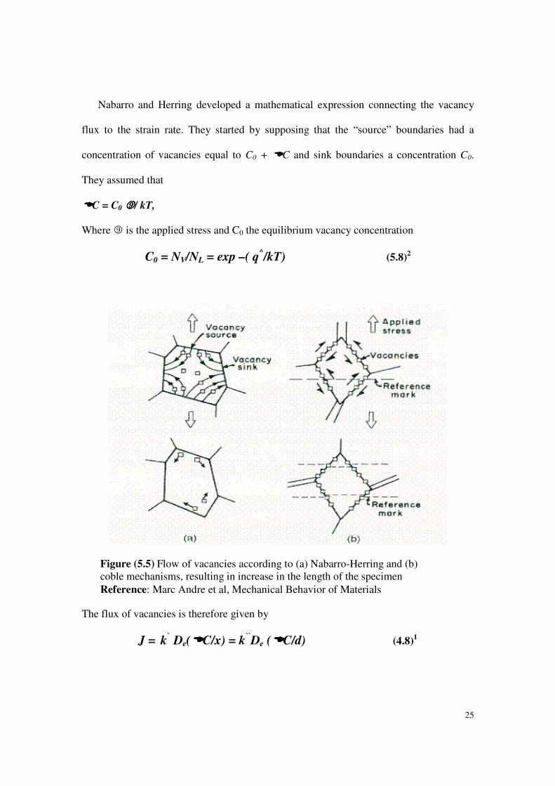
Nabarro and Herring proposed the mechanism shown schematically in Figure (5.5).

It involves the flux of vacancies inside the grain. The vacancies move in such a way as to

produce an increase in length of the grain along the direction of applied (tensile) stress.

Hence, the vacancies move from the top and bottom region in the figure to the lateral

regions of the grain. The boundaries perpendicular (or close to perpendicular) to the

loading direction are distended and are sources of vacancies. The boundaries close to

parallel to the loading direction act as sinks.1

25

Nabarro and Herring developed a mathematical expression connecting the vacancy

flux to the strain rate. They started by supposing that the “source” boundaries had a

concentration of vacancies equal to C0 + ��C and sink boundaries a concentration C0.

They assumed that

��C = C0 9999/ kT,

Where 9 is the applied stress and C0 the equilibrium vacancy concentration

C0 = NV/NL = exp –( q^/kT) (5.8)2

The flux of vacancies is therefore given by

J = k

` De(��C/x) = k

``De (��C/d) (4.8)

1

Figure (5.5) Flow of vacancies according to (a) Nabarro-Herring and (b) coble mechanisms, resulting in increase in the length of the specimen


26

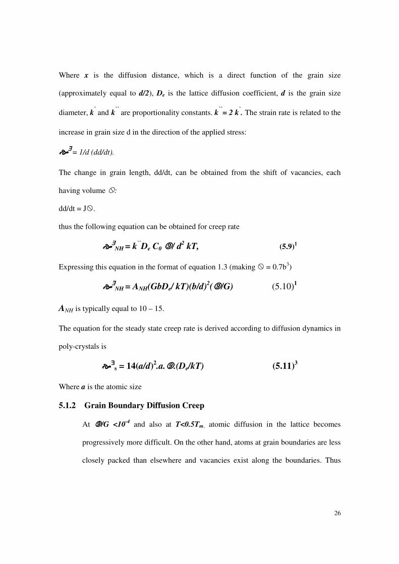
Where x is the diffusion distance, which is a direct function of the grain size

(approximately equal to d/2), De is the lattice diffusion coefficient, d is the grain size

diameter, k` and k

`` are proportionality constants. k

``= 2 k

`. The strain rate is related to the

increase in grain size d in the direction of the applied stress:

��∃∃∃∃

= 1/d (dd/dt).

The change in grain length, dd/dt, can be obtained from the shift of vacancies, each

having volume �:

dd/dt = J�.

thus the following equation can be obtained for creep rate

��∃∃∃∃

NH = k``De C0 9999/ d

2 kT, (5.9)

1

Expressing this equation in the format of equation 1.3 (making � = 0.7b3)

��∃∃∃∃

NH = ANH(GbDe/ kT)(b/d)2(9999/G) (5.10)1

ANH is typically equal to 10 – 15.

The equation for the steady state creep rate is derived according to diffusion dynamics in

poly-crystals is

��∃∃∃∃

s = 14(a/d)2.a.9999.(De/kT) (5.11)

3

Where a is the atomic size

5.1.2 Grain Boundary Diffusion Creep

At 9999/G <10-4 and also at T<0.5Tm, atomic diffusion in the lattice becomes

progressively more difficult. On the other hand, atoms at grain boundaries are less

closely packed than elsewhere and vacancies exist along the boundaries. Thus

27

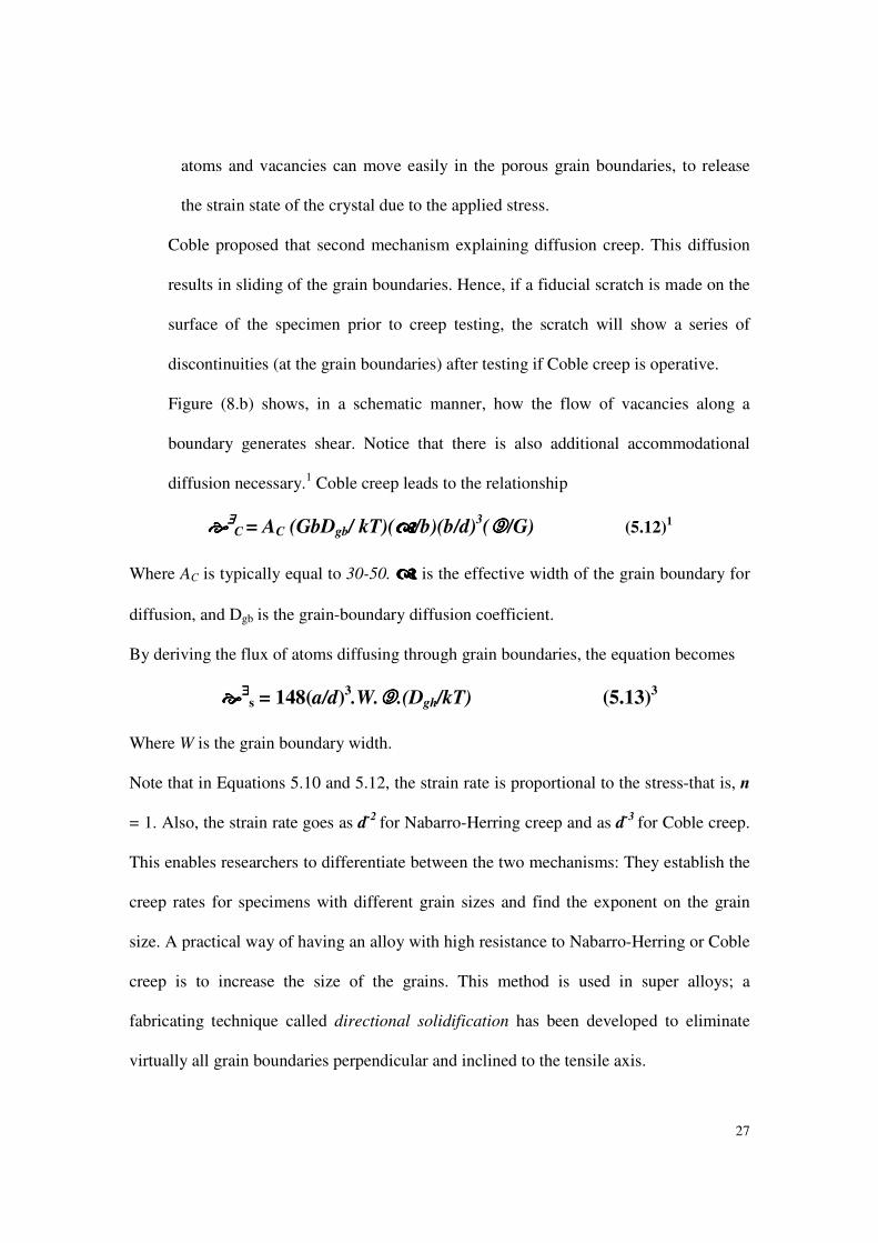
atoms and vacancies can move easily in the porous grain boundaries, to release

the strain state of the crystal due to the applied stress.

Coble proposed that second mechanism explaining diffusion creep. This diffusion

results in sliding of the grain boundaries. Hence, if a fiducial scratch is made on the

surface of the specimen prior to creep testing, the scratch will show a series of

discontinuities (at the grain boundaries) after testing if Coble creep is operative.

Figure (8.b) shows, in a schematic manner, how the flow of vacancies along a

boundary generates shear. Notice that there is also additional accommodational

diffusion necessary.1 Coble creep leads to the relationship

��∃∃∃∃

C = AC (GbDgb/ kT)(��/b)(b/d)3(9999/G) (5.12)

1

Where AC is typically equal to 30-50. �� is the effective width of the grain boundary for

diffusion, and Dgb is the grain-boundary diffusion coefficient.

By deriving the flux of atoms diffusing through grain boundaries, the equation becomes

��∃∃∃∃

s = 148(a/d)3.W.9999.(Dgh/kT) (5.13)

3

Where W is the grain boundary width.

Note that in Equations 5.10 and 5.12, the strain rate is proportional to the stress-that is, n

= 1. Also, the strain rate goes as d-2 for Nabarro-Herring creep and as d-3 for Coble creep.

This enables researchers to differentiate between the two mechanisms: They establish the

creep rates for specimens with different grain sizes and find the exponent on the grain

size. A practical way of having an alloy with high resistance to Nabarro-Herring or Coble

creep is to increase the size of the grains. This method is used in super alloys; a

fabricating technique called directional solidification has been developed to eliminate

virtually all grain boundaries perpendicular and inclined to the tensile axis.

28

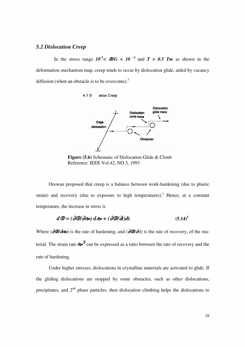
5.2 Dislocation Creep

In the stress range 10-5< 9999/G < 10 -3 and T > 0.5 Tm as shown in the

deformation mechanism map, creep tends to occur by dislocation glide, aided by vacancy

diffusion (when an obstacle is to be overcome).3

Orowan proposed that creep is a balance between work-hardening (due to plastic

strain) and recovery (due to exposure to high temperatures).1 Hence, at a constant

temperature, the increase in stress is

d9999 = (∂∂∂∂9999/∂∂∂∂��) d�� + (∂∂∂∂9999/∂∂∂∂t)dt, (5.14)1

Where (∂∂∂∂9999/∂∂∂∂��) is the rate of hardening, and (∂∂∂∂9999/∂∂∂∂ t) is the rate of recovery, of the ma-

terial. The strain rate ��∃∃∃∃ can be expressed as a ratio between the rate of recovery and the

rate of hardening.

Under higher stresses, dislocations in crystalline materials are activated to glide. If

the gliding dislocations are stopped by some obstacles, such as other dislocations,

precipitates, and 2nd phase particles, then dislocation climbing helps the dislocations to

Figure (5.6) Schematic of Dislocation Glide & Climb Reference: IEEE Vol.42, NO.3, 1993

29

overcome the obstacles and continue their gliding as shown in figure (5.6). Therefore

dislocation motion controlled creep deformation occurs by both dislocations gliding and

climbing. Dislocation gliding, viz, crystallographic slip deformation, produces almost all

the creep strain, while dislocation climbing controls the creep rate, because the

dislocation gliding rate is much faster than atomic diffusion rate which controls

dislocation climbing.

A creep model based on the mechanisms of dislocation climbing and atomic

diffusion predicts the steady state creep rate to be proportional to the third power of

stress. However creep experiments show that the exponent of stress ranges from 1 to 8.

Therefore the steady state creep is generally presented by power –low equation:

��∃∃∃∃

s=A(DeGb/kT)(9999/G)n

= B9999n.exp(-Q/kT) (5.15)

3

The term A incorporates the various parameters and proportionality coefficients

B is determined by the slip magnitude & direction of a dislocation in crystal.

Equation (5.15) shows the power- low relation between steady state creep and stress for

creep controlled by dislocation gliding and climbing. This model can be more generally

used for both dislocation creep (n µµµµ 2) and diffusion creep (n =1).

When 9/G>10-3, dislocation gliding dominates over atomic diffusion effect

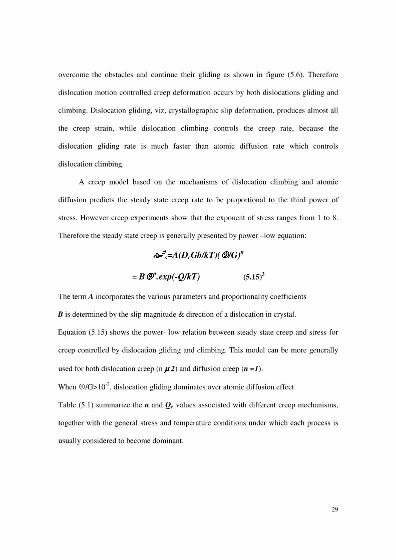
Table (5.1) summarize the n and Qc values associated with different creep mechanisms,

together with the general stress and temperature conditions under which each process is

usually considered to become dominant.

30

Creep Process Temp. Stress n value Qc value

High temperature dislocation >~0.7Tm Intermediate/high >3 ~QSD

Low temperature dislocation ~0.4 to~0.7Tm Intermediate/high >3 Qcore***

High temp. diffusional creep

(Nabarro-Herring)

>~0.7Tm Low ~1 QSD

Low temp. diffusional creep

(Coble creep)

~0.4 to

~0.7Tm

Low ~1 QGB

*** Qcore is the activation energy for self-diffusion along dislocation cores (Qcore=QGB)

5.3 Grain-Boundary Sliding And Supperplasticity

Grain-boundary sliding usually does not play an important role during primary or

secondary creep. However, in tertiary creep it does contribute to the initiation and

propagation of intercrystalline cracks. in fact it has some contribution to creep in primary.

Because of that this creep mechanism is not shown in figure (5.1), though temperature

and stress conditions are similar to that of diffusion creep. There is a good relation

between the activation energy of creep deformation ( mainly due to grain boundary

sliding ) and of the lattice self-diffusion. Therefore, the sliding is considered as diffusion

controlled process, even though the creep deformation is caused by grain boundary

sliding.

Another deformation process to which it contributes significantly is super

plasticity; it is thought that most of the deformation in super plastic forming takes place

Table (5.1) Values of n and QC associated with dislocation and diffusional creep (pure metal)

Reference: R.W.Evans et al, Introduction to Creep

31

by grain-boundary sliding.

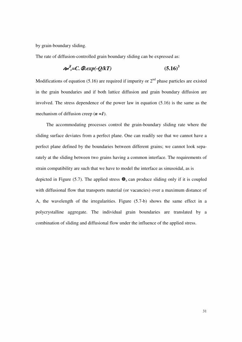
The rate of diffusion-controlled grain boundary sliding can be expressed as:

��∃∃∃∃

s=C.9999.exp(-Q/kT) (5.16)3

Modifications of equation (5.16) are required if impurity or 2nd phase particles are existed

in the grain boundaries and if both lattice diffusion and grain boundary diffusion are

involved. The stress dependence of the power law in equation (5.16) is the same as the

mechanism of diffusion creep (n =1).

The accommodating processes control the grain-boundary sliding rate where the

sliding surface deviates from a perfect plane. One can readily see that we cannot have a

perfect plane defined by the boundaries between different grains; we cannot look sepa-

rately at the sliding between two grains having a common interface. The requirements of

strain compatibility are such that we have to model the interface as sinusoidal, as is

depicted in Figure (5.7). The applied stress �a can produce sliding only if it is coupled

with diffusional flow that transports material (or vacancies) over a maximum distance of

A, the wavelength of the irregularities. Figure (5.7-b) shows the same effect in a

polycrystalline aggregate. The individual grain boundaries are translated by a

combination of sliding and diffusional flow under the influence of the applied stress.

32

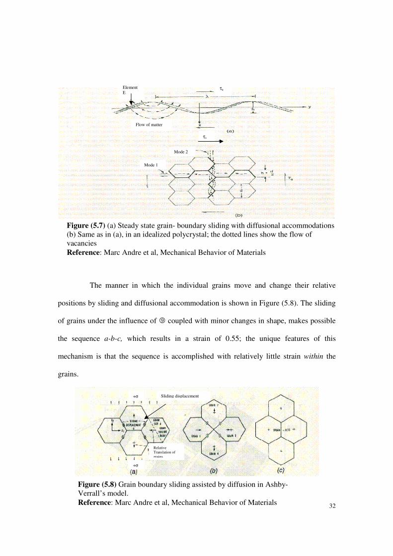
The manner in which the individual grains move and change their relative

positions by sliding and diffusional accommodation is shown in Figure (5.8). The sliding

of grains under the influence of 9 coupled with minor changes in shape, makes possible

the sequence a-b-c, which results in a strain of 0.55; the unique features of this

mechanism is that the sequence is accomplished with relatively little strain within the

grains.

Figure (5.8) Grain boundary sliding assisted by diffusion in Ashby-Verrall’s model.


Figure (5.7) (a) Steady state grain- boundary sliding with diffusional accommodations (b) Same as in (a), in an idealized polycrystal; the dotted lines show the flow of vacancies


Element E

Flow of matter

τa

τa

Mode 2

Mode 1

+σ

+σ

Relative Translation of grains

Sliding displacement

33

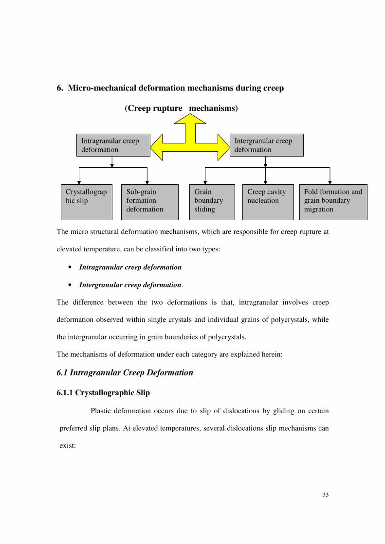
6. Micro-mechanical deformation mechanisms during creep

(Creep rupture mechanisms)

The micro structural deformation mechanisms, which are responsible for creep rupture at

elevated temperature, can be classified into two types:

• Intragranular creep deformation

• Intergranular creep deformation.

The difference between the two deformations is that, intragranular involves creep

deformation observed within single crystals and individual grains of polycrystals, while

the intergranular occurring in grain boundaries of polycrystals.

The mechanisms of deformation under each category are explained herein:

6.1 Intragranular Creep Deformation

6.1.1 Crystallographic Slip

Plastic deformation occurs due to slip of dislocations by gliding on certain

preferred slip plans. At elevated temperatures, several dislocations slip mechanisms can

exist:

Intragranular creep deformation

Intergranular creep deformation

Fold formation and grain boundary migration

Creep cavity nucleation

Grain boundary sliding

Sub-grain formation deformation

Crystallographic slip

34

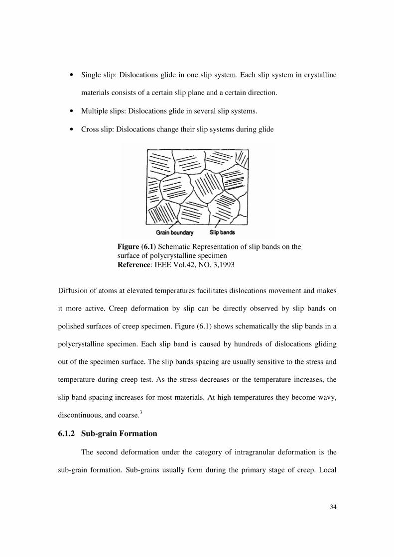
• Single slip: Dislocations glide in one slip system. Each slip system in crystalline

materials consists of a certain slip plane and a certain direction.

• Multiple slips: Dislocations glide in several slip systems.

• Cross slip: Dislocations change their slip systems during glide

Diffusion of atoms at elevated temperatures facilitates dislocations movement and makes

it more active. Creep deformation by slip can be directly observed by slip bands on

polished surfaces of creep specimen. Figure (6.1) shows schematically the slip bands in a

polycrystalline specimen. Each slip band is caused by hundreds of dislocations gliding

out of the specimen surface. The slip bands spacing are usually sensitive to the stress and

temperature during creep test. As the stress decreases or the temperature increases, the

slip band spacing increases for most materials. At high temperatures they become wavy,

discontinuous, and coarse.3

6.1.2 Sub-grain Formation

The second deformation under the category of intragranular deformation is the

sub-grain formation. Sub-grains usually form during the primary stage of creep. Local

Figure (6.1) Schematic Representation of slip bands on the surface of polycrystalline specimen

Reference: IEEE Vol.42, NO. 3,1993

35

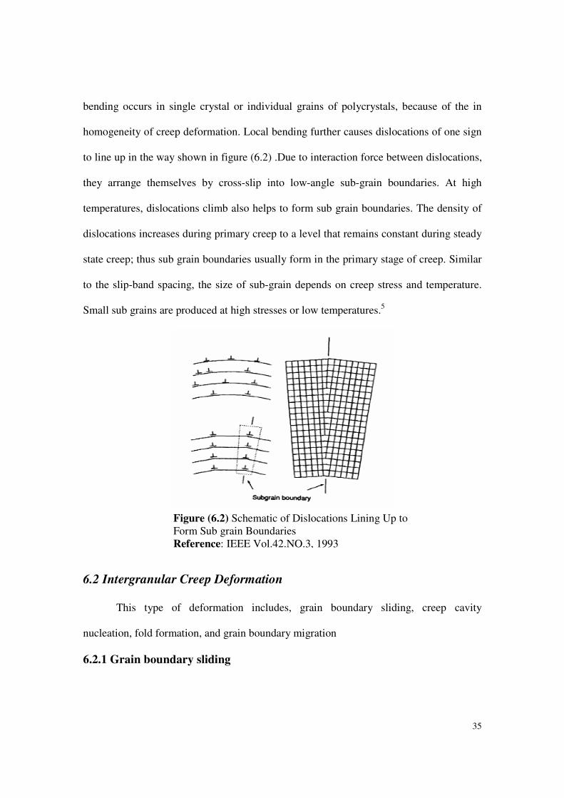
bending occurs in single crystal or individual grains of polycrystals, because of the in

homogeneity of creep deformation. Local bending further causes dislocations of one sign

to line up in the way shown in figure (6.2) .Due to interaction force between dislocations,

they arrange themselves by cross-slip into low-angle sub-grain boundaries. At high

temperatures, dislocations climb also helps to form sub grain boundaries. The density of

dislocations increases during primary creep to a level that remains constant during steady

state creep; thus sub grain boundaries usually form in the primary stage of creep. Similar

to the slip-band spacing, the size of sub-grain depends on creep stress and temperature.

Small sub grains are produced at high stresses or low temperatures.5

6.2 Intergranular Creep Deformation

This type of deformation includes, grain boundary sliding, creep cavity

nucleation, fold formation, and grain boundary migration

6.2.1 Grain boundary sliding

Figure (6.2) Schematic of Dislocations Lining Up to Form Sub grain Boundaries Reference: IEEE Vol.42.NO.3, 1993

36

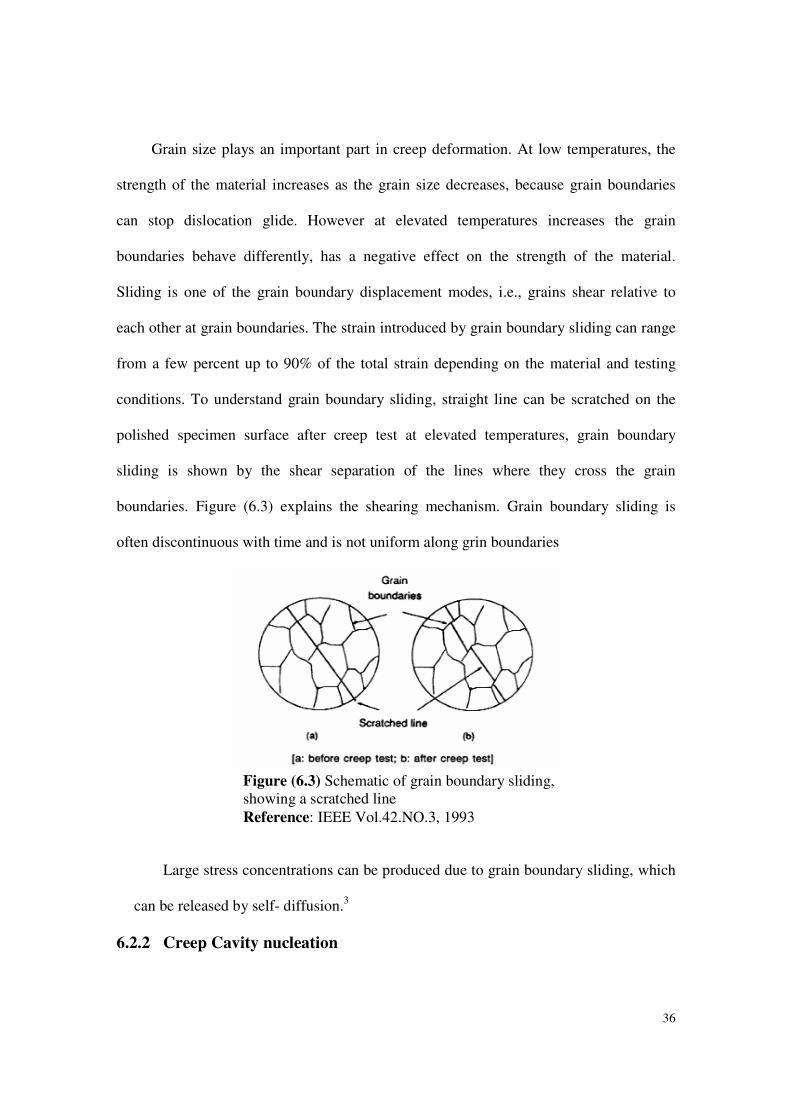
Grain size plays an important part in creep deformation. At low temperatures, the

strength of the material increases as the grain size decreases, because grain boundaries

can stop dislocation glide. However at elevated temperatures increases the grain

boundaries behave differently, has a negative effect on the strength of the material.

Sliding is one of the grain boundary displacement modes, i.e., grains shear relative to

each other at grain boundaries. The strain introduced by grain boundary sliding can range

from a few percent up to 90% of the total strain depending on the material and testing

conditions. To understand grain boundary sliding, straight line can be scratched on the

polished specimen surface after creep test at elevated temperatures, grain boundary

sliding is shown by the shear separation of the lines where they cross the grain

boundaries. Figure (6.3) explains the shearing mechanism. Grain boundary sliding is

often discontinuous with time and is not uniform along grin boundaries

Large stress concentrations can be produced due to grain boundary sliding, which

can be released by self- diffusion.3

6.2.2 Creep Cavity nucleation

Figure (6.3) Schematic of grain boundary sliding, showing a scratched line

Reference: IEEE Vol.42.NO.3, 1993

37

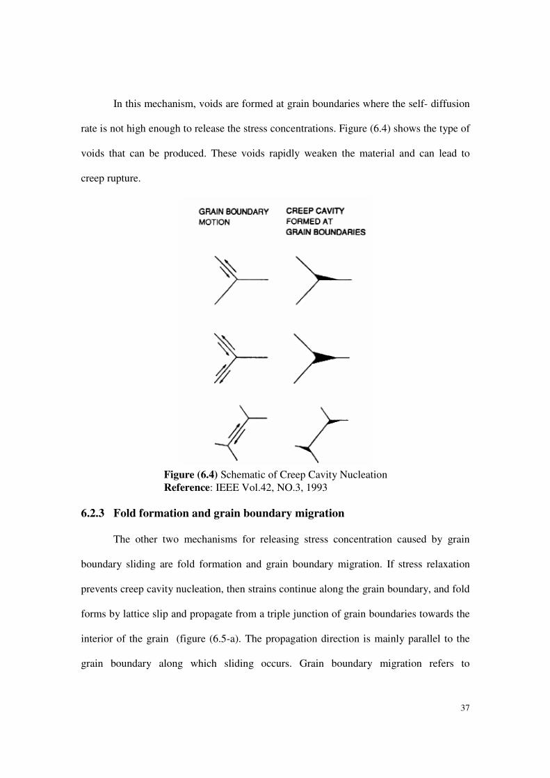
In this mechanism, voids are formed at grain boundaries where the self- diffusion

rate is not high enough to release the stress concentrations. Figure (6.4) shows the type of

voids that can be produced. These voids rapidly weaken the material and can lead to

creep rupture.

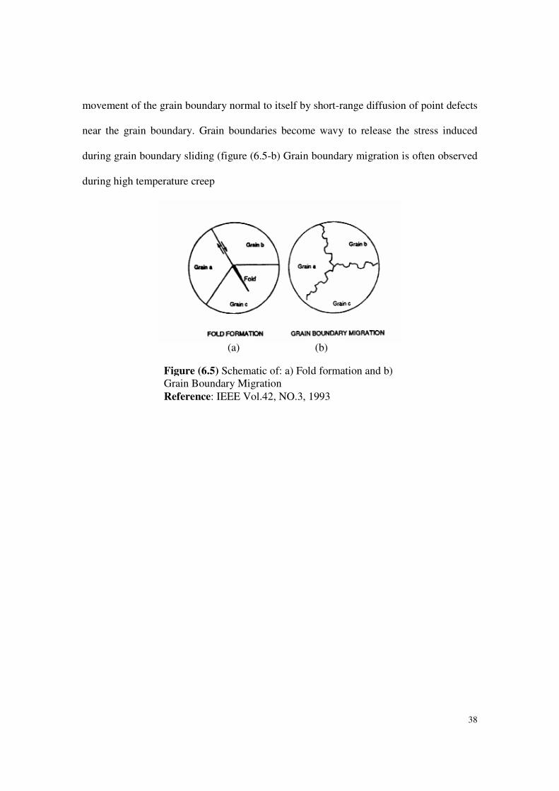
6.2.3 Fold formation and grain boundary migration

The other two mechanisms for releasing stress concentration caused by grain

boundary sliding are fold formation and grain boundary migration. If stress relaxation

prevents creep cavity nucleation, then strains continue along the grain boundary, and fold

forms by lattice slip and propagate from a triple junction of grain boundaries towards the

interior of the grain (figure (6.5-a). The propagation direction is mainly parallel to the

grain boundary along which sliding occurs. Grain boundary migration refers to

Figure (6.4) Schematic of Creep Cavity Nucleation

Reference: IEEE Vol.42, NO.3, 1993

38

movement of the grain boundary normal to itself by short-range diffusion of point defects

near the grain boundary. Grain boundaries become wavy to release the stress induced

during grain boundary sliding (figure (6.5-b) Grain boundary migration is often observed

during high temperature creep

Figure (6.5) Schematic of: a) Fold formation and b) Grain Boundary Migration

Reference: IEEE Vol.42, NO.3, 1993

(a) (b)

39

7. Creep Life Assessment

There is a need to assess the remaining life of industrial components, which are

subjected to steady load and high temperatures environment. Particularly when the

components have been in service for long time. Lifetime of a component is a function of

stress and temperature. The design stress is generally the relevant rupture stress factored

to allow for material variability, some variation in plant operating conditions, corrosion,

and weldments in structure. Many plants operate safely beyond their design life. Thus

two distinct parts of service life can be defined.4

a) The original design life which can typically be 100000hr (11.4 years);

b) the safe economic life.

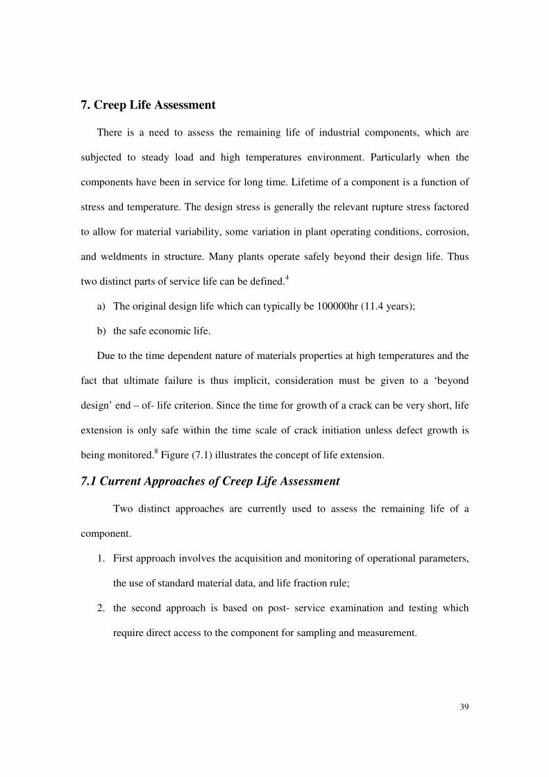
Due to the time dependent nature of materials properties at high temperatures and the

fact that ultimate failure is thus implicit, consideration must be given to a ‘beyond

design’ end – of- life criterion. Since the time for growth of a crack can be very short, life

extension is only safe within the time scale of crack initiation unless defect growth is

being monitored.8 Figure (7.1) illustrates the concept of life extension.

7.1 Current Approaches of Creep Life Assessment

Two distinct approaches are currently used to assess the remaining life of a

component.

1. First approach involves the acquisition and monitoring of operational parameters,

the use of standard material data, and life fraction rule;

2. the second approach is based on post- service examination and testing which

require direct access to the component for sampling and measurement.

40

7.1 Approach (a); operational condition monitoring

Operating temperatures and pressures are monitored and recorded. A combination

of the operational parameters, standard creep rupture data and inverse design stress

calculations which, in association with simple damage summation rules, produce a

preliminary estimate of the remaining life. Some assumptions are included in the

estimation of remaining life, which lead to uncertainties of the results. Therefore this

approach does not provide a realistic basis on which to base life extension or planning for

component replacement.4

7.1 Approach (b); methods base on post-service examination sampling and

calculation

These techniques are more accurate than the operational monitoring approach

since they don not rely on standard materials data. These methods position the component

materials within the standard data scattered either:

Figure (7.1) Life extension of high temperature equipment Reference: Journal of strain analysis Vol.29 NO 3, 1994

41

• by measuring its properties and hence providing a refined prediction based on

stress and temperature records and damage summation rules, or

• Direct assessment of the extend of damage experienced by the component as a

result of actual service exposure.

Both destructive and non-destructive methods can be used. Component type, location of

critical area, and economic factors control the method used, either destructive or non-

destructive. The main methods of the second approach are:

1. Creep and rupture testing;

2. Methods based on assessment of micro structural degradation and cavitations

damage;

3. Methods based on component strain measurement

7.1.1 Creep and rupture testing

Several extrapolation methods have been developed to predict creep life based on

tests conducted over a shorter period. There are more than 30 methods can be used in this

concern. However, three most common methods are the Larson –Milller, Manson-

Haferd, and Sherby- Dorn.1

7.1.1.1 Larson- Miller Method:

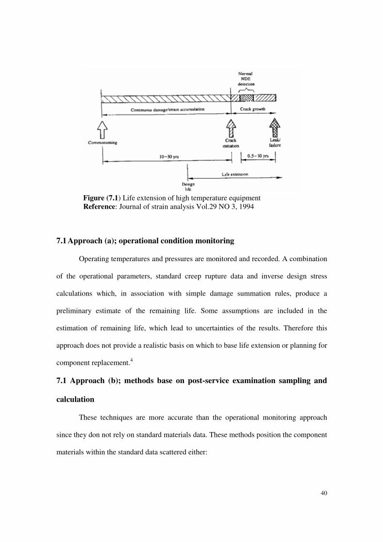
This method simply correlates the temperature T (in kelvins) with the time

to failure tr, at a constant engineering stress 9999. The Larson – Miller equation has the

form

mCtr =+Τ )(log (7.1 )1

Where C is a constant that depends on the alloy, m is a parameter that depends on the

stress, and rupture time. According to that equation, if C is known for a particular alloy,

42

m can be easily found in a single test. So one can find the rupture time at any

temperature, as long as the same engineering stress is applied. Figure (7.2) graphically

represents the equation

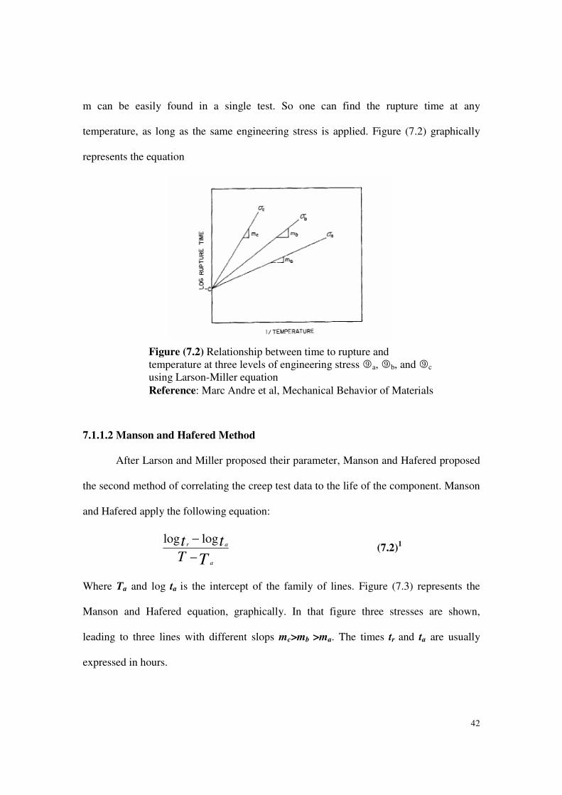
7.1.1.2 Manson and Hafered Method

After Larson and Miller proposed their parameter, Manson and Hafered proposed

the second method of correlating the creep test data to the life of the component. Manson

and Hafered apply the following equation:

T

tt

a

ar

T −

− loglog (7.2)

1

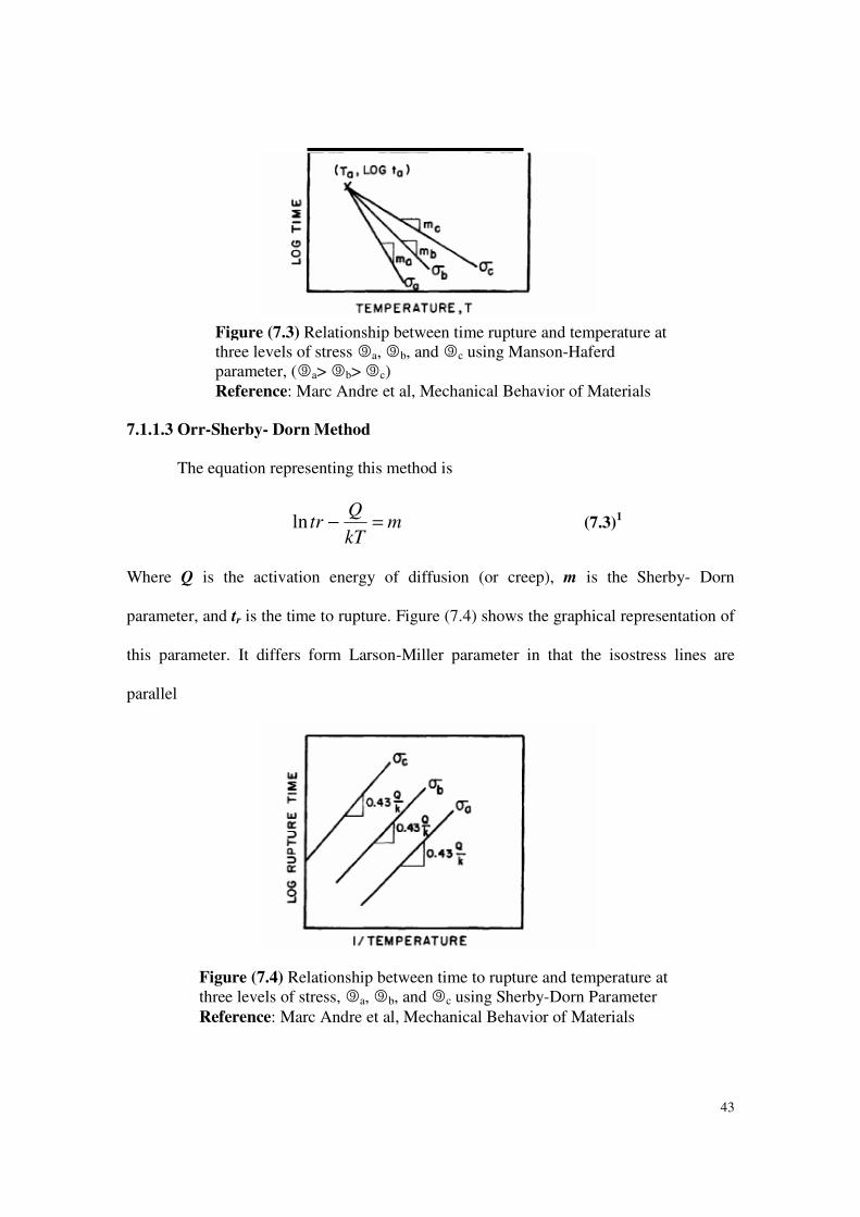
Where Ta and log ta is the intercept of the family of lines. Figure (7.3) represents the

Manson and Hafered equation, graphically. In that figure three stresses are shown,

leading to three lines with different slops mc>mb >ma. The times tr and ta are usually

expressed in hours.

Figure (7.2) Relationship between time to rupture and temperature at three levels of engineering stress 9a, 9b, and 9c using Larson-Miller equation


43

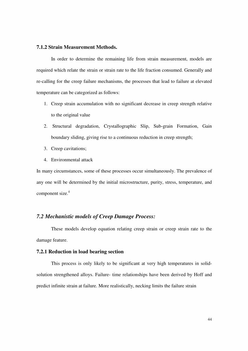
7.1.1.3 Orr-Sherby- Dorn Method

The equation representing this method is

mkT

Qtr =−ln (7.3)

1

Where Q is the activation energy of diffusion (or creep), m is the Sherby- Dorn

parameter, and tr is the time to rupture. Figure (7.4) shows the graphical representation of

this parameter. It differs form Larson-Miller parameter in that the isostress lines are

parallel

Figure (7.3) Relationship between time rupture and temperature at three levels of stress 9a, 9b, and 9c using Manson-Haferd parameter, (9a> 9b> 9c)


Figure (7.4) Relationship between time to rupture and temperature at three levels of stress, 9a, 9b, and 9c using Sherby-Dorn Parameter


44

7.1.2 Strain Measurement Methods.

In order to determine the remaining life from strain measurement, models are

required which relate the strain or strain rate to the life fraction consumed. Generally and

re-calling for the creep failure mechanisms, the processes that lead to failure at elevated

temperature can be categorized as follows:

1. Creep strain accumulation with no significant decrease in creep strength relative

to the original value

2. Structural degradation, Crystallographic Slip, Sub-grain Formation, Gain

boundary sliding, giving rise to a continuous reduction in creep strength;

3. Creep cavitations;

4. Environmental attack

In many circumstances, some of these processes occur simultaneously. The prevalence of

any one will be determined by the initial microstructure, purity, stress, temperature, and

component size.4

7.2 Mechanistic models of Creep Damage Process:

These models develop equation relating creep strain or creep strain rate to the

damage feature.

7.2.1 Reduction in load bearing section

This process is only likely to be significant at very high temperatures in solid-

solution strengthened alloys. Failure- time relationships have been derived by Hoff and

predict infinite strain at failure. More realistically, necking limits the failure strain

45

7.2.2 Micro structural degradation

High temperature creep resistance arises from the finely dispersed precipitates.

Creep rate is primarily dependent on the interparticle spacing and the associated

mechanisms by which dislocations overcome the particles. Under these conditions, it is

possible to relate the creep rate,�., to the structural state via a modified Norton low

��. =A1(9999-99990)

n f (T) (7.4 )4

Where A1 and n are material parameters, and T is temperature. 99990 is regarded as a

threshold stress having a value close to the Orwan stress, i.e.

99990 ~ λαµ /b

Where µ is the shear modulus, b is the burgers vector, and α is a particle – dislocation

interaction coefficient. By specifying a failure criteria e.g. critical level of strain, equation

(7.4) provides a means of relating strain or strain rate measured to component lifetime.

7.2.3 Cavitation damage

Creep cavities nucleate and grow predominantly on grain boundaries oriented

normal to the maximum principle stress. Numerous controlling mechanisms have been

suggested to creep cavitation- namely vacancy flow, power –law growth, and constrained

cavity growth. Power- law growth and diffusion control are most likely at high strain rate

or low cavity spacing. Creep rate is described as

��.= B9999

n/(1-Ac)

n (7.5)

4

Where Ac is the fraction of cavitating grain boundaries and B and n are material

constants. Same here, a failure criterion must be specified

46

7.2.4 Effect of Environment

Creep in aggressive environments, including air, normally leads to changes in

rupture life and ductility. The low alloy ferritic steel, for example, form oxides, which

spell during exposure, reducing the load bearing section and accelerating, creep. The

kinetics of creep and oxidation in these materials and such that metal loss measured after

creep fracture increases with decreasing temperature in iso-stress test. Consequently if the

oxide is non-load bearing it is relatively simple task to predict the creep curve as a

function of stress and temperature using the appropriate oxidation data. At service

temperatures the oxide is often strongly adherent and is likely to bear some of the load

because its inherent creep resistance is grater generally than the metal. In this case, the

rate of attack is controlled no longer by inward diffusion of oxygen but by the frequency

of surface cracking. The extent of oxidation is thus dependent on strain rate as well as

time. Under these circumstances the rate of oxidation becomes linear with time, even

though the oxidation kinetics are parabolic, and the specimen size is important in

determining life expectancy.

7.3 Phenomenological models

From an engineering viewpoint, the mechanics of creep damage, tertiary creep,

and fracture have developed as a continuum mechanical approach. Damage is described

by a generalized scalar parameter,ω , which varies from zero at the start of life to unity at

failure. Both damage and strain are assumed to increase as functions of stress,σ ,

temperature, T, and the current state of the damage, so that for uniaxial tension the creep

rate and damage rate are expressed as

�� = A9999n/(1 - ω )

n (7.6)

4

47

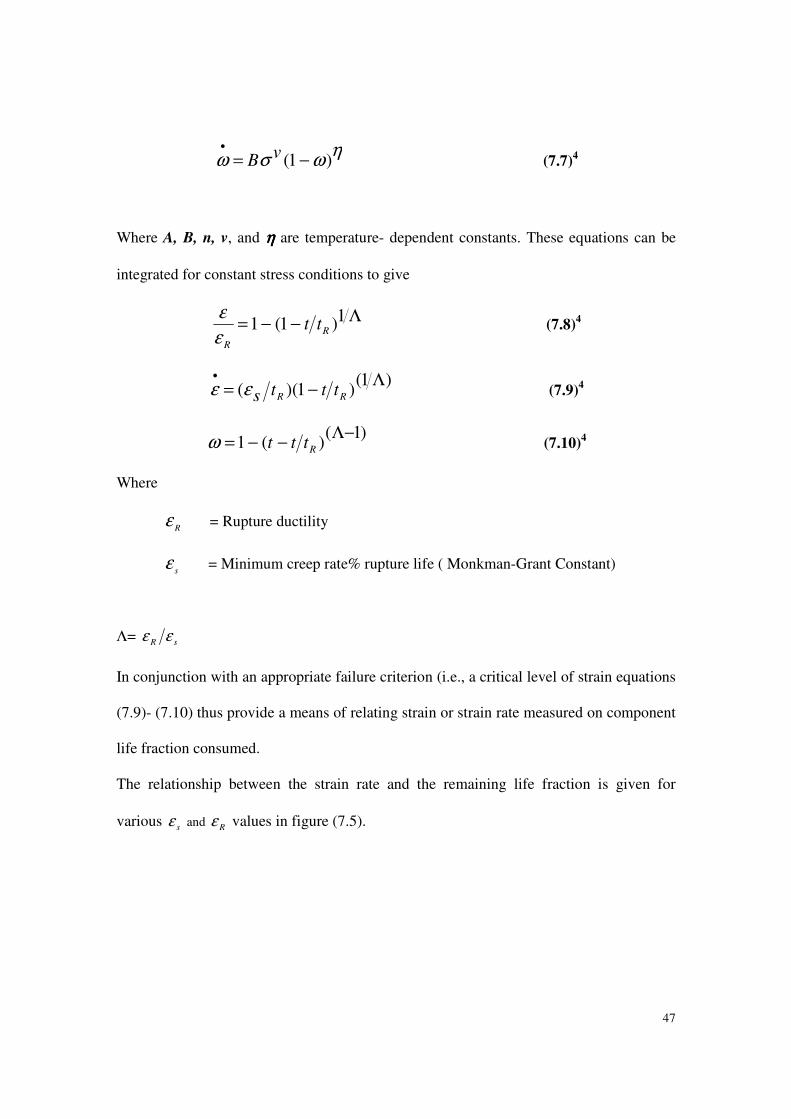
ηωσω )1( −=

• vB (7.7)

4

Where A, B, n, v, and ηηηη are temperature- dependent constants. These equations can be

integrated for constant stress conditions to give

Λ−−= 1)1(1R

R

ttε

ε (7.8)

4

)1()1)((

Λ−=

•

RRtttsεε (7.9)

4

)1()(1

−Λ−−=

Rtttω (7.10)

4

Where

R

ε = Rupture ductility

s

ε = Minimum creep rate% rupture life ( Monkman-Grant Constant)

Λ= sR εε

In conjunction with an appropriate failure criterion (i.e., a critical level of strain equations

(7.9)- (7.10) thus provide a means of relating strain or strain rate measured on component

life fraction consumed.

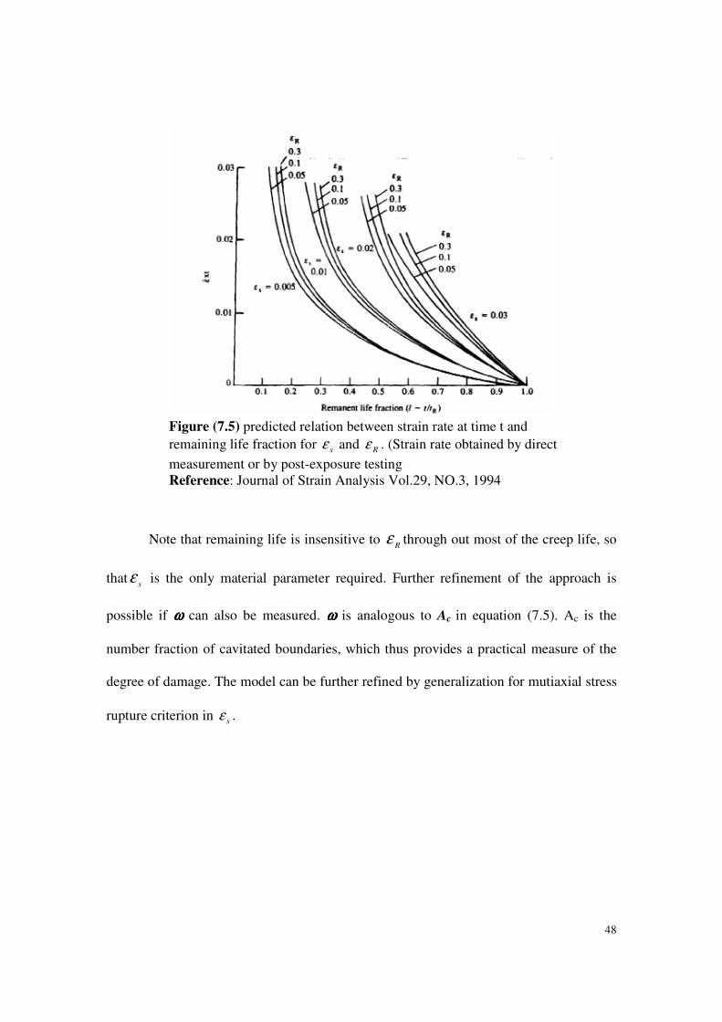
The relationship between the strain rate and the remaining life fraction is given for

various sε and

Rε values in figure (7.5).

48

Note that remaining life is insensitive to R

ε through out most of the creep life, so

thats

ε is the only material parameter required. Further refinement of the approach is

possible if ωωωω can also be measured. ωωωω is analogous to Ac in equation (7.5). Ac is the

number fraction of cavitated boundaries, which thus provides a practical measure of the

degree of damage. The model can be further refined by generalization for mutiaxial stress

rupture criterion in sε .

Figure (7.5) predicted relation between strain rate at time t and

remaining life fraction for sε and Rε . (Strain rate obtained by direct

measurement or by post-exposure testing Reference: Journal of Strain Analysis Vol.29, NO.3, 1994

49

8. Material Specifications

As mentioned in the introduction part the tubes are used in very high temperature

applications, so the material should resist high temperature oxidation as well as

mechanical degradation. The typical specifications are summarized below.

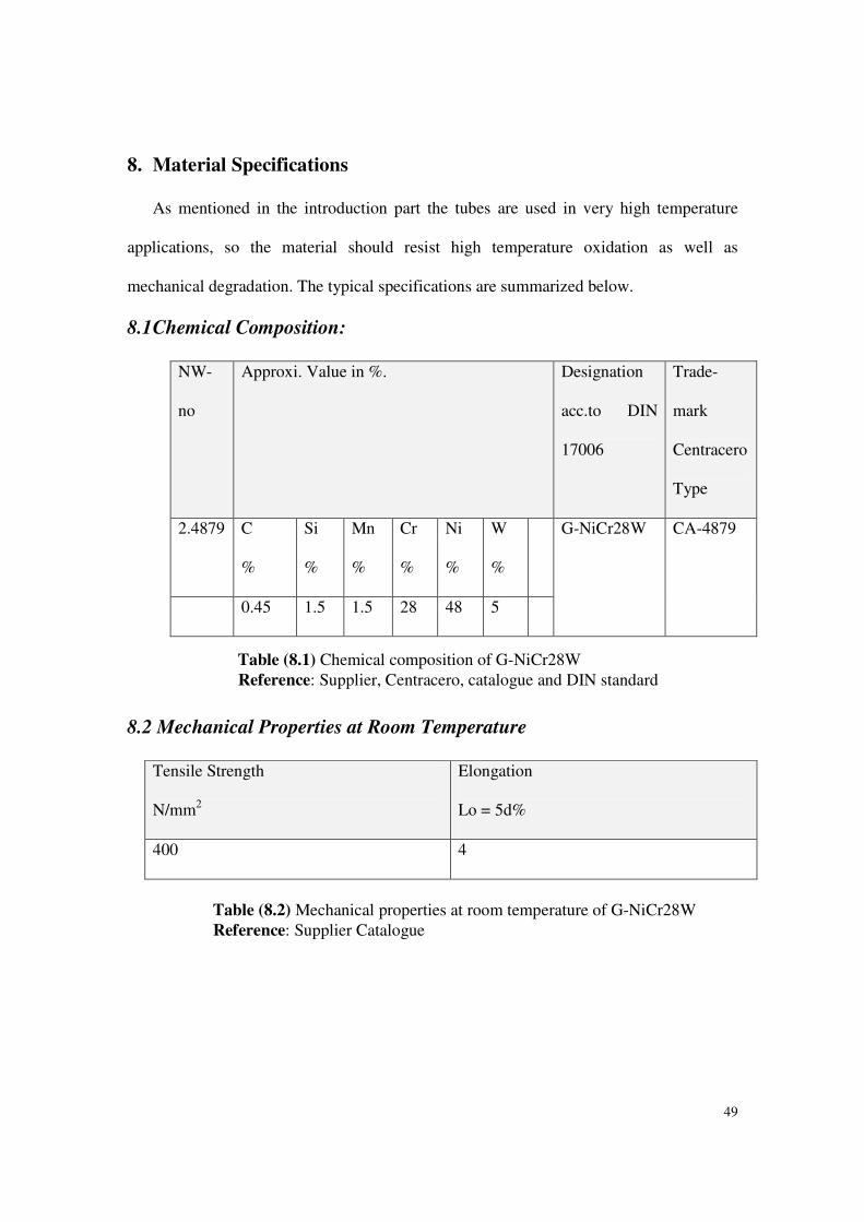
8.1 Chemical Composition:

NW-

no

Approxi. Value in %. Designation

acc.to DIN

17006

Trade-

mark

Centracero

Type

2.4879 C

%

Si

%

Mn

%

Cr

%

Ni

%

W

%

G-NiCr28W CA-4879

0.45 1.5 1.5 28 48 5

8.2 Mechanical Properties at Room Temperature

Tensile Strength

N/mm2

Elongation

Lo = 5d%

400 4

Table (8.1) Chemical composition of G-NiCr28W

Reference: Supplier, Centracero, catalogue and DIN standard

Table (8.2) Mechanical properties at room temperature of G-NiCr28W

Reference: Supplier Catalogue

50

8.3 Physical Properties

Density

g/cm3

Shrinkage

%

Thermal

Conductivity

W/moC

Specific

heat

20oCJ/goC

Thermal expansion

between 20oC

10-6m/mmoC

Highest

application

temp. in air

400oC 800oC 1000oC

8.2 2.5 11.0 0.502 14.5 16 17 1150

Table (8.3) Physical properties of G-NiCr28W Reference: Supplier Catalogue

51

9. Experimental procedure

Because of the alloy in question is a special one there was no enough data

available on reference books or papers. So in addition to the accelerated creep test other

tests such as impact test, tensile test, hardness test and micro-structural examination have

been conducted to get the properties of that alloy at room temperature as well as at

elevated temperature

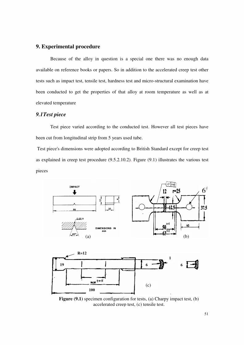
9.1 Test piece

Test piece varied according to the conducted test. However all test pieces have

been cut from longitudinal strip from 5 years used tube.

Test piece's dimensions were adopted according to British Standard except for creep test

as explained in creep test procedure (9.5.2.10.2). Figure (9.1) illustrates the various test

pieces

100

1

6 6

R=12

19

(c)

(a) (b)

Figure (9.1) specimen configuration for tests, (a) Charpy impact test, (b) accelerated creep test, (c) tensile test.

6�

52

It is worth mentioning that it was not easy to manufacture the required specimen as

special tools were used to machine them.

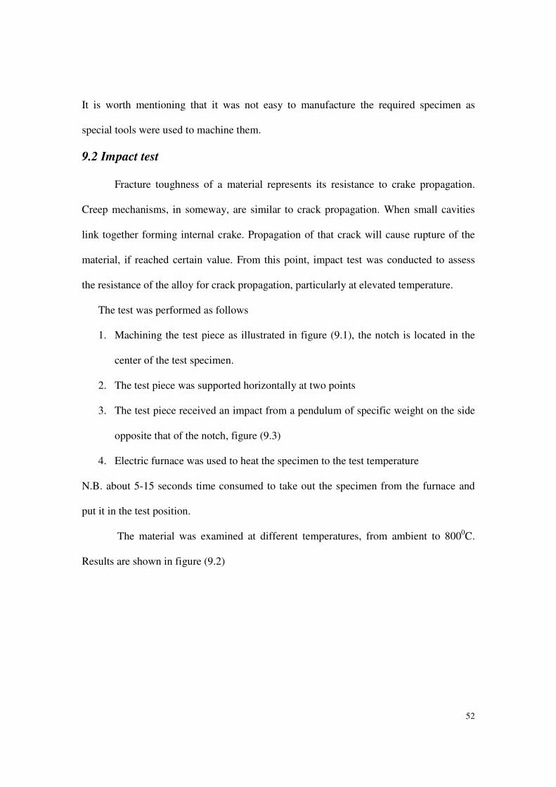
9.2 Impact test

Fracture toughness of a material represents its resistance to crake propagation.

Creep mechanisms, in someway, are similar to crack propagation. When small cavities

link together forming internal crake. Propagation of that crack will cause rupture of the

material, if reached certain value. From this point, impact test was conducted to assess

the resistance of the alloy for crack propagation, particularly at elevated temperature.

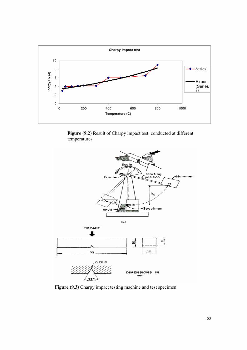
The test was performed as follows

1. Machining the test piece as illustrated in figure (9.1), the notch is located in the

center of the test specimen.

2. The test piece was supported horizontally at two points

3. The test piece received an impact from a pendulum of specific weight on the side

opposite that of the notch, figure (9.3)

4. Electric furnace was used to heat the specimen to the test temperature

N.B. about 5-15 seconds time consumed to take out the specimen from the furnace and

put it in the test position.

The material was examined at different temperatures, from ambient to 8000C.

Results are shown in figure (9.2)

53

Charpy Impact test

0

2

4

6

8

10

0 200 400 600 800 1000

Temperature (C)

En

erg

y C

v (

J)

Series1

Expon.(Series1)

Figure (9.2) Result of Charpy impact test, conducted at different temperatures

Figure (9.3) Charpy impact testing machine and test specimen

54

9.3 Hardness test

Hardness is one of the most important properties of metals. The reason is because

it relates to several other properties of metal, such as strength, brittleness, and ductility.

Therefore by measuring the hardness we are indirectly measuring the strength, the

brittleness, and the ductility of that metal.

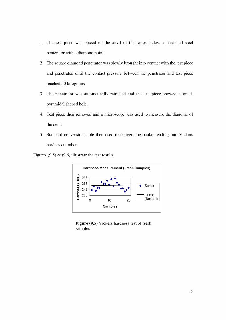
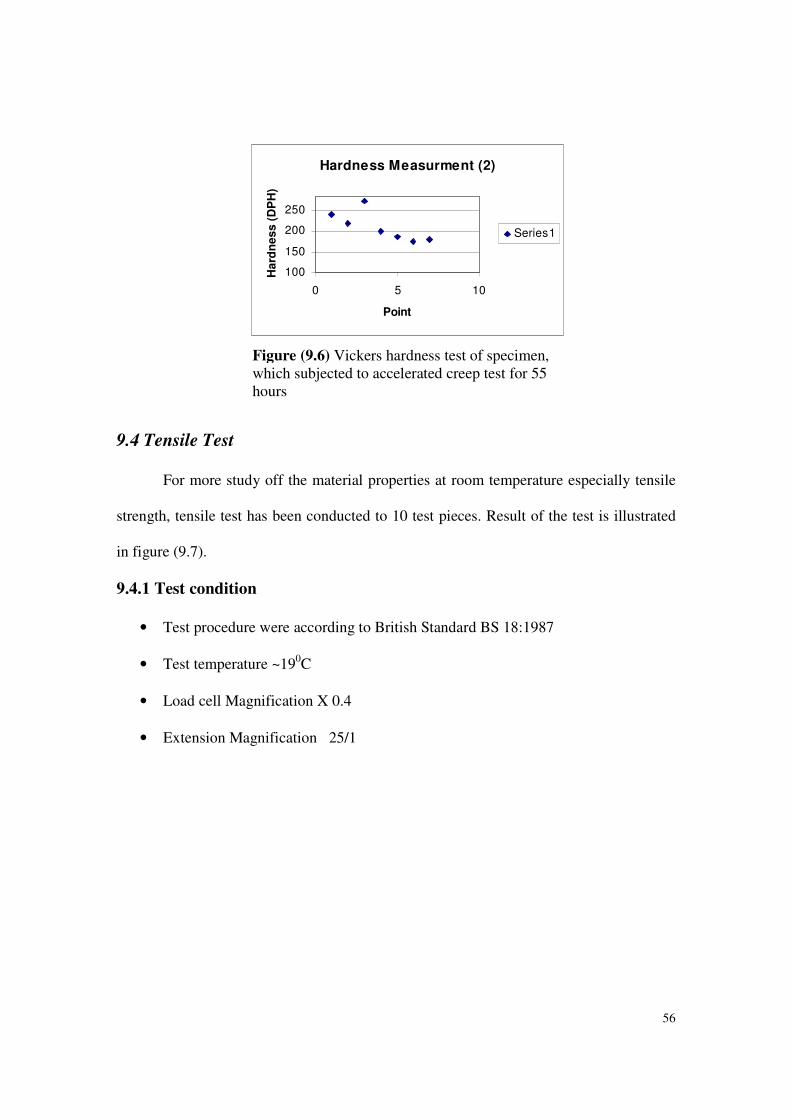
Vickers hardness test has been conducted on two different samples. First sample

was fresh samples and the second was unbroken specimen in accelerated creep test,

which lasted for 55 hours, as will be explained later.

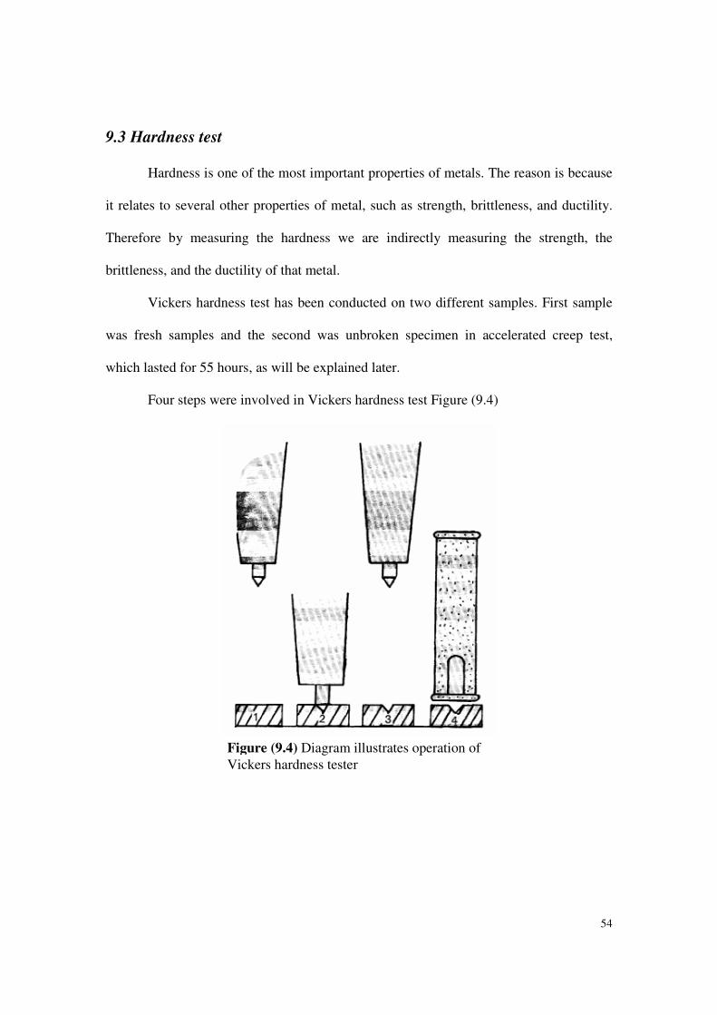
Four steps were involved in Vickers hardness test Figure (9.4)

Figure (9.4) Diagram illustrates operation of

Vickers hardness tester

55

1. The test piece was placed on the anvil of the tester, below a hardened steel

penterator with a diamond point

2. The square diamond penetrator was slowly brought into contact with the test piece

and penetrated until the contact pressure between the penetrator and test piece

reached 50 kilograms

3. The penetrator was automatically retracted and the test piece showed a small,

pyramidal shaped hole.

4. Test piece then removed and a microscope was used to measure the diagonal of

the dent.

5. Standard conversion table then used to convert the ocular reading into Vickers

hardness number.

Figures (9.5) & (9.6) illustrate the test results

Hardness Measurement (Fresh Samples)

225

245

265

285

0 10 20

Samples

Hard

ness (

DP

H)

Series1

Linear(Series1)

Figure (9.5) Vickers hardness test of fresh samples

56

Hardness Measurment (2)

100

150

200

250

0 5 10

Point

Ha

rdn

es

s (

DP

H)

Series1

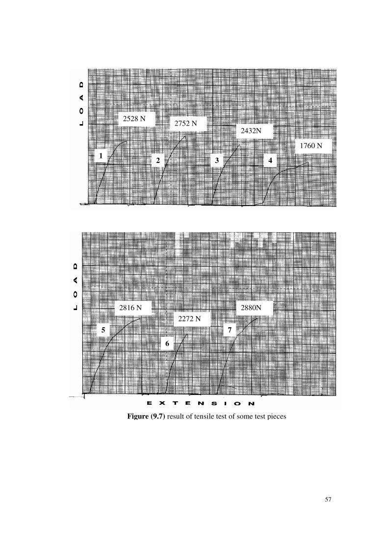
9.4 Tensile Test

For more study off the material properties at room temperature especially tensile

strength, tensile test has been conducted to 10 test pieces. Result of the test is illustrated

in figure (9.7).

9.4.1 Test condition

• Test procedure were according to British Standard BS 18:1987

• Test temperature ~190C

• Load cell Magnification X 0.4

• Extension Magnification 25/1

Figure (9.6) Vickers hardness test of specimen, which subjected to accelerated creep test for 55 hours

57

Figure (9.7) result of tensile test of some test pieces

2528 N 2752 N

2432N

1760 N

2880N

2272 N

2816 N

1 2 3 4

5

6

7

58

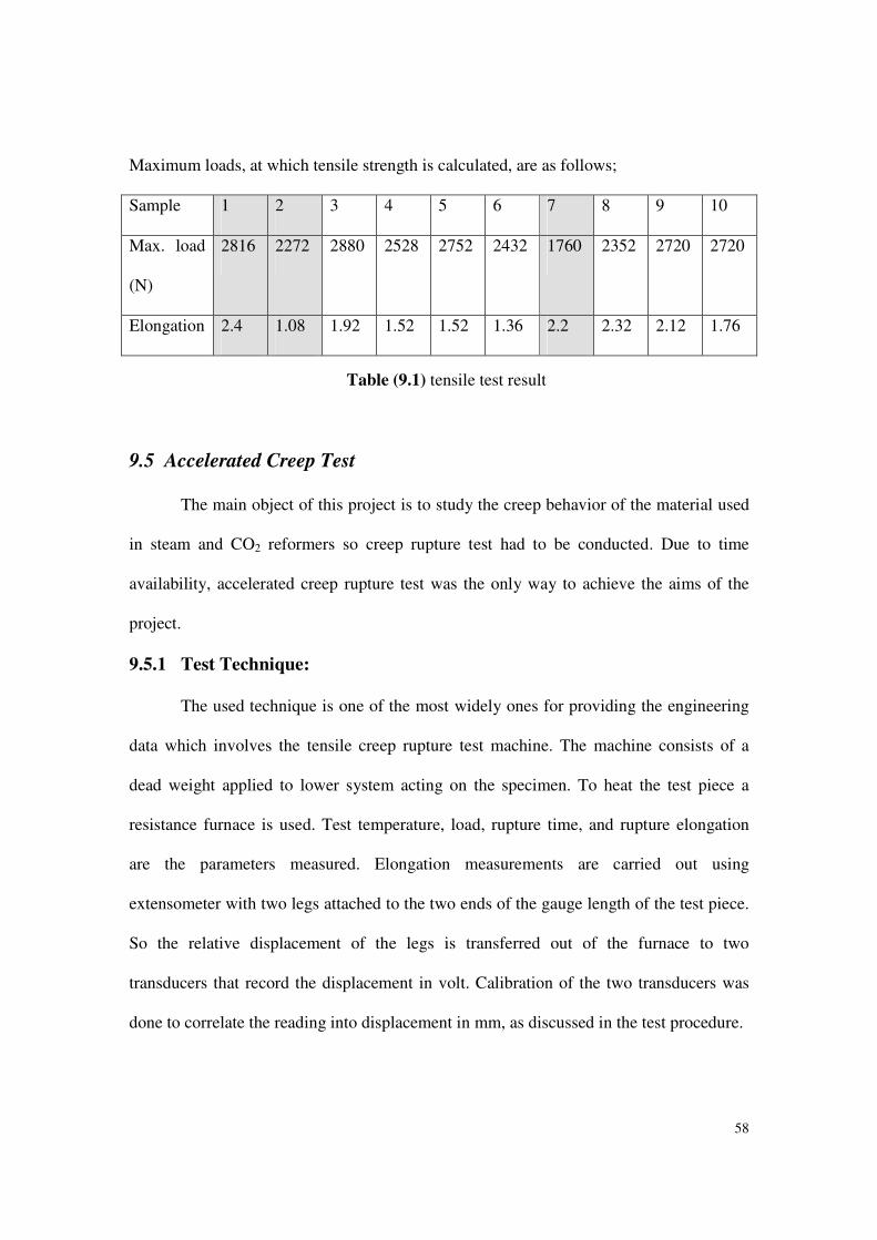
Maximum loads, at which tensile strength is calculated, are as follows;

Sample 1 2 3 4 5 6 7 8 9 10

Max. load

(N)

2816 2272 2880 2528 2752 2432 1760 2352 2720 2720

Elongation 2.4 1.08 1.92 1.52 1.52 1.36 2.2 2.32 2.12 1.76

9.5 Accelerated Creep Test

The main object of this project is to study the creep behavior of the material used

in steam and CO2 reformers so creep rupture test had to be conducted. Due to time

availability, accelerated creep rupture test was the only way to achieve the aims of the

project.

9.5.1 Test Technique:

The used technique is one of the most widely ones for providing the engineering

data which involves the tensile creep rupture test machine. The machine consists of a

dead weight applied to lower system acting on the specimen. To heat the test piece a

resistance furnace is used. Test temperature, load, rupture time, and rupture elongation

are the parameters measured. Elongation measurements are carried out using

extensometer with two legs attached to the two ends of the gauge length of the test piece.

So the relative displacement of the legs is transferred out of the furnace to two

transducers that record the displacement in volt. Calibration of the two transducers was

done to correlate the reading into displacement in mm, as discussed in the test procedure.

Table (9.1) tensile test result

59

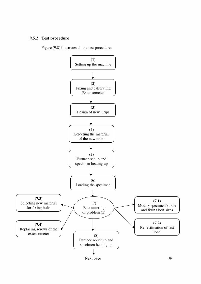
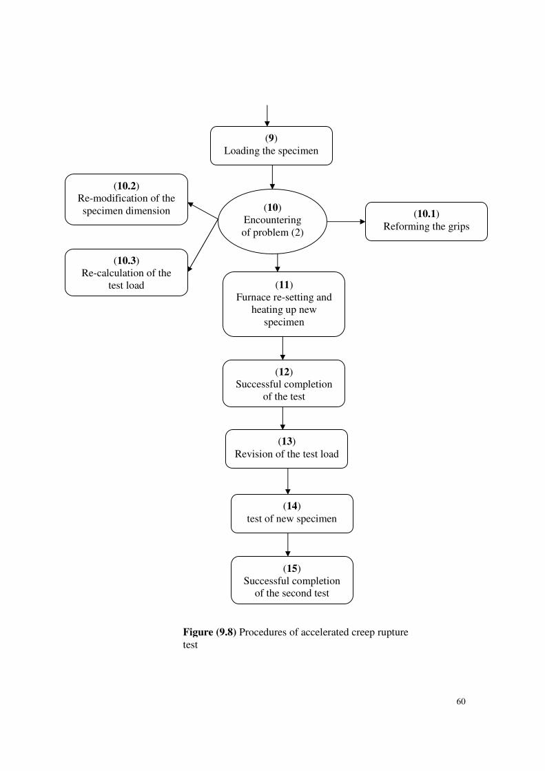
9.5.2 Test procedure

Figure (9.8) illustrates all the test procedures

(1) Setting up the machine

(2) Fixing and calibrating

Extensometer

(3) Design of new Grips

(4) Selecting the material

of the new grips

(5) Furnace set up and

specimen heating up

(7) Encountering

of problem (1)

(7.1) Modify specimen’s hole

and fixing bolt sizes

(7.3) Selecting new material

for fixing bolts

(7.4) Replacing screws of the

extensometer

(6) Loading the specimen

(8) Furnace re-set up and specimen heating up

(7.2) Re- estimation of test

load

Next page

60

(9) Loading the specimen

(10) Encountering of problem (2)

(10.1) Reforming the grips

(10.2) Re-modification of the specimen dimension

(10.3) Re-calculation of the

test load (11) Furnace re-setting and

heating up new specimen

(12) Successful completion

of the test

(13)

Revision of the test load

(14)

test of new specimen

(15) Successful completion

of the second test

Figure (9.8) Procedures of accelerated creep rupture test

61

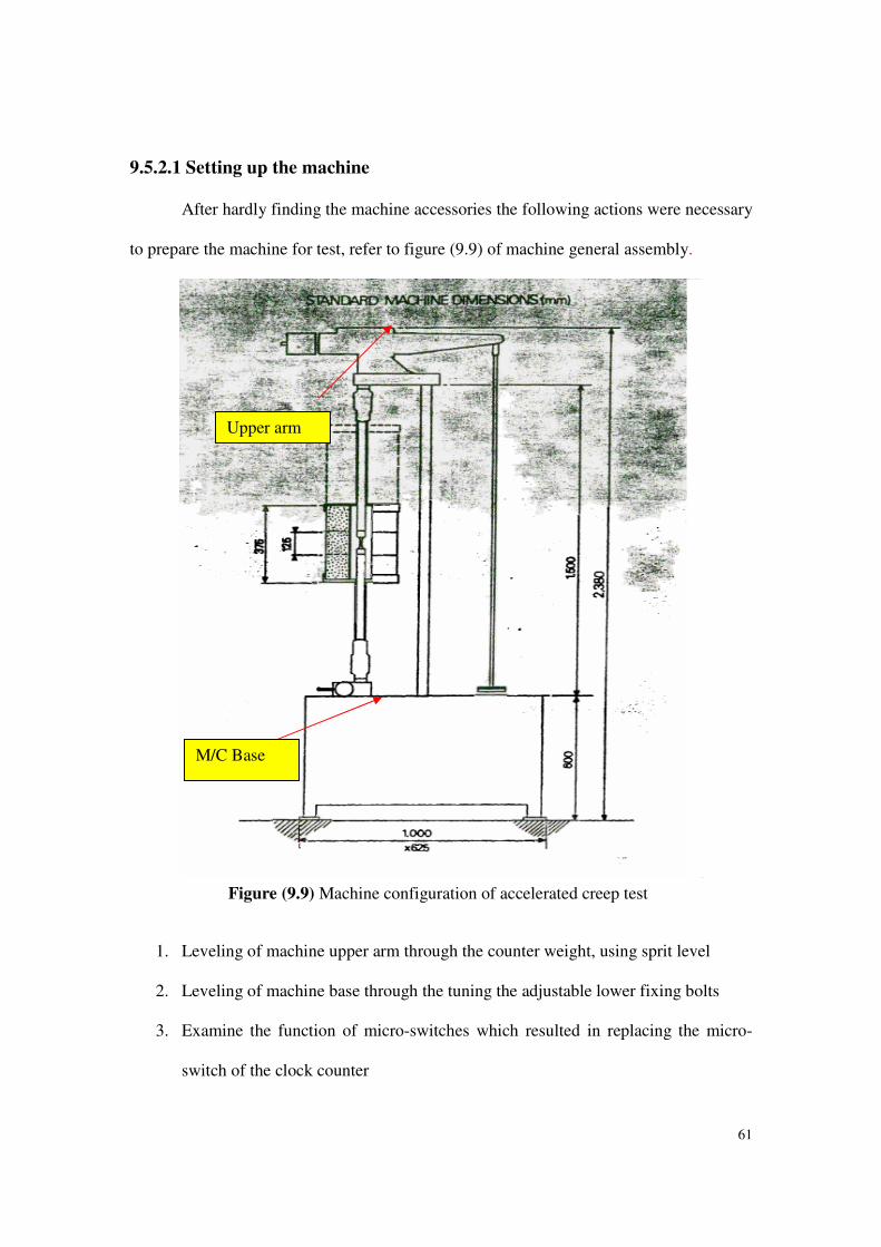
9.5.2.1 Setting up the machine

After hardly finding the machine accessories the following actions were necessary

to prepare the machine for test, refer to figure (9.9) of machine general assembly.

1. Leveling of machine upper arm through the counter weight, using sprit level

2. Leveling of machine base through the tuning the adjustable lower fixing bolts

3. Examine the function of micro-switches which resulted in replacing the micro-

switch of the clock counter

Upper arm

M/C Base

Figure (9.9) Machine configuration of accelerated creep test

62

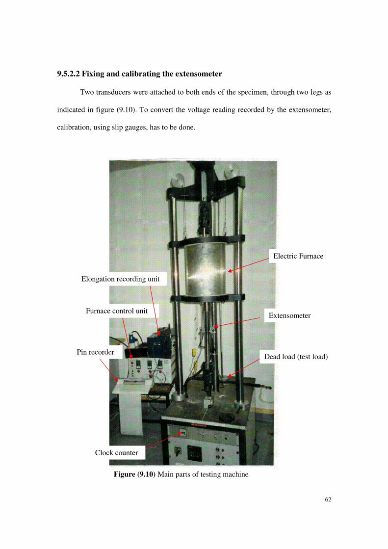
9.5.2.2 Fixing and calibrating the extensometer

Two transducers were attached to both ends of the specimen, through two legs as

indicated in figure (9.10). To convert the voltage reading recorded by the extensometer,

calibration, using slip gauges, has to be done.

Electric Furnace

Extensometer

Pin recorder

Furnace control unit

Clock counter

Elongation recording unit

Dead load (test load)

Figure (9.10) Main parts of testing machine

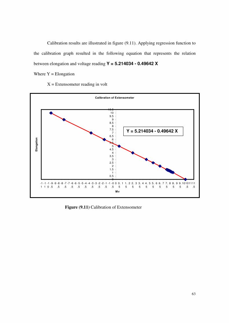
63

Calibration results are illustrated in figure (9.11). Applying regression function to

the calibration graph resulted in the following equation that represents the relation

between elongation and voltage reading Y = 5.214034 - 0.49642 X

Where Y = Elongation

X = Extensometer reading in volt

Calibration of Extensometer

0

0.5

1

1.5

2

2.5

3

3.5

4

4.5

5

5.5

6

6.5

7

7.5

8

8.5

9

9.5

10

10.5

-1

1

-1

1

-1

0

-9

.5

-9 -8

.5

-8 -7

.5

-7 -6

.5

-6 -5

.5

-5 -4

.5

-4 -3

.5

-3 -2

.5

-2 -1

.5

-1 -0

.5

0 0.

5

1 1.

5

2 2.

5

3 3.

5

4 4.

5

5 5.

5

6 6.

5

7 7.

5

8 8.

5

9 9.

5

1010

.5

1111

.5

Mv

Elo

ng

ati

on

Figure (9.11) Calibration of Extensometer

Y = 5.214034 - 0.49642 X

64

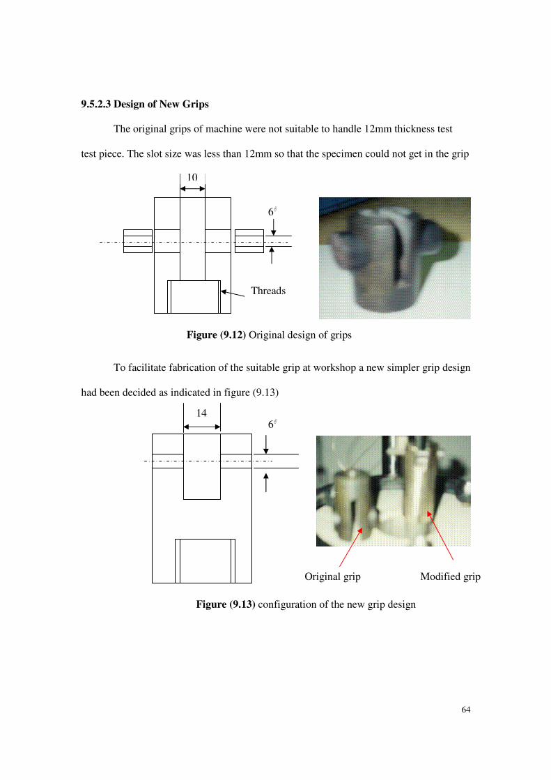
9.5.2.3 Design of New Grips

The original grips of machine were not suitable to handle 12mm thickness test

test piece. The slot size was less than 12mm so that the specimen could not get in the grip

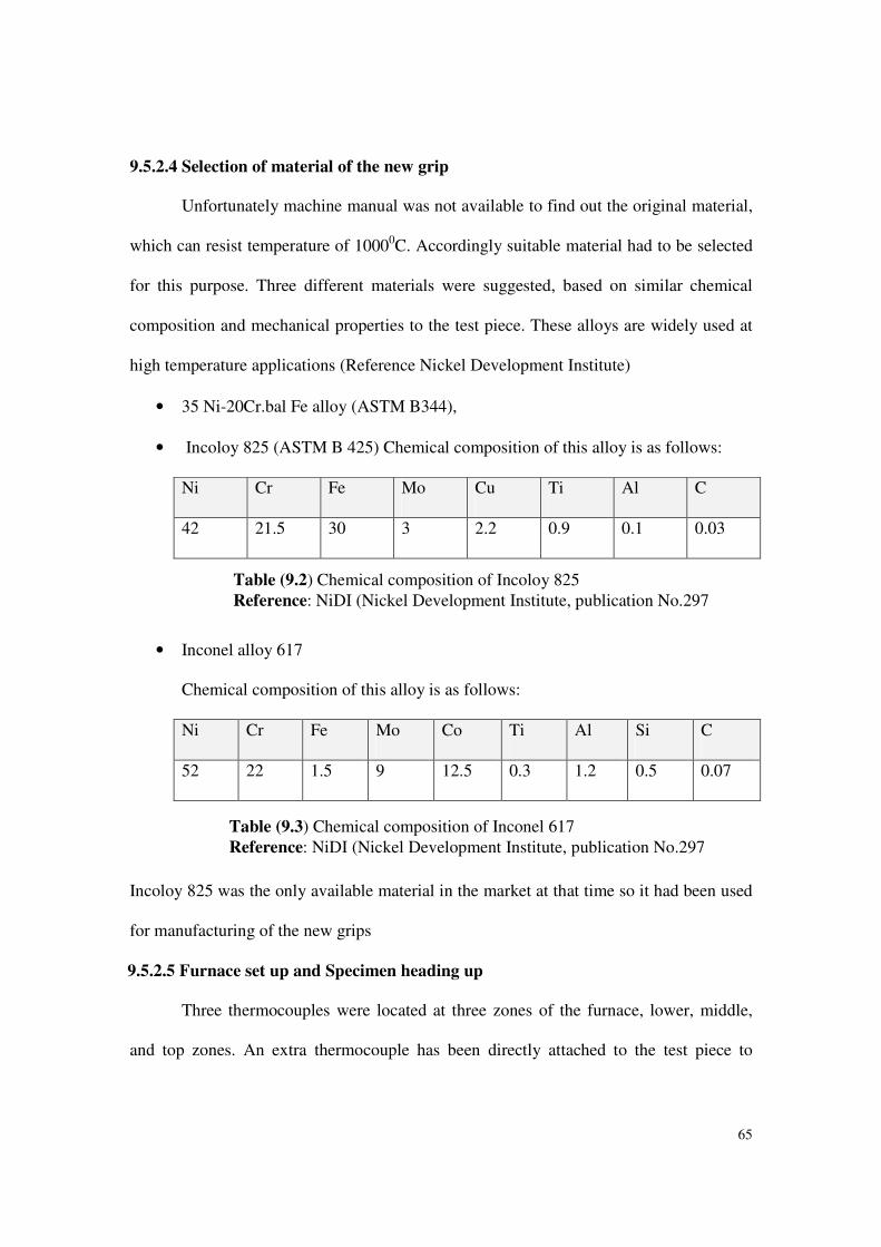
To facilitate fabrication of the suitable grip at workshop a new simpler grip design

had been decided as indicated in figure (9.13)

10

6�

Figure (9.12) Original design of grips

Threads

14 6�

Figure (9.13) configuration of the new grip design

Original grip Modified grip

65

9.5.2.4 Selection of material of the new grip

Unfortunately machine manual was not available to find out the original material,

which can resist temperature of 10000C. Accordingly suitable material had to be selected

for this purpose. Three different materials were suggested, based on similar chemical

composition and mechanical properties to the test piece. These alloys are widely used at

high temperature applications (Reference Nickel Development Institute)

• 35 Ni-20Cr.bal Fe alloy (ASTM B344),

• Incoloy 825 (ASTM B 425) Chemical composition of this alloy is as follows:

Ni Cr Fe Mo Cu Ti Al C

42 21.5 30 3 2.2 0.9 0.1 0.03

• Inconel alloy 617

Chemical composition of this alloy is as follows:

Ni Cr Fe Mo Co Ti Al Si C

52 22 1.5 9 12.5 0.3 1.2 0.5 0.07

Incoloy 825 was the only available material in the market at that time so it had been used

for manufacturing of the new grips

9.5.2.5 Furnace set up and Specimen heading up

Three thermocouples were located at three zones of the furnace, lower, middle,

and top zones. An extra thermocouple has been directly attached to the test piece to

Table (9.2) Chemical composition of Incoloy 825

Reference: NiDI (Nickel Development Institute, publication No.297

Table (9.3) Chemical composition of Inconel 617

Reference: NiDI (Nickel Development Institute, publication No.297

66

measure its actual temperature. The attached thermocouple to the test piece was

connected to pin recorder and the temperature was continuously plotted on chart. Heating

the test piece usually took 24 hours to reach the test temperature (1000 0C) in addition to

one hour at least at the test temperature.

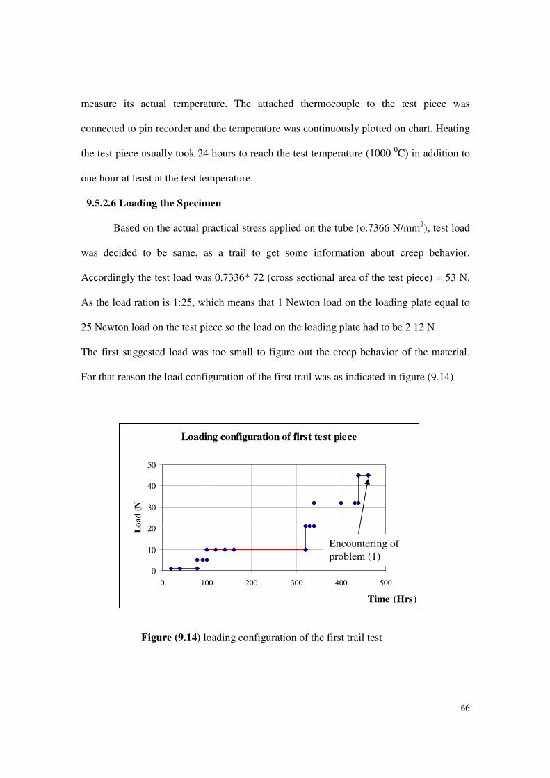
9.5.2.6 Loading the Specimen

Based on the actual practical stress applied on the tube (o.7366 N/mm2), test load

was decided to be same, as a trail to get some information about creep behavior.

Accordingly the test load was 0.7336* 72 (cross sectional area of the test piece) = 53 N.

As the load ration is 1:25, which means that 1 Newton load on the loading plate equal to

25 Newton load on the test piece so the load on the loading plate had to be 2.12 N

The first suggested load was too small to figure out the creep behavior of the material.

For that reason the load configuration of the first trail was as indicated in figure (9.14)

Loading configuration of first test piece

0

10

20

30

40

50

0 100 200 300 400 500

Time (Hrs)

Lo

ad

(N

)

Figure (9.14) loading configuration of the first trail test

Encountering of

problem (1)

67

9.5.2.7 Encountering of problem (1)

After increasing the load to (45) the loading plate touched the machine base and

hence the clock counter stopped. By checking the test piece condition after cooling down

the furnace the following have been observed.

1. Rupture of the test piece fixing bolts upper and lower ones

2. Fusion of the ruptured part of fixing bolts with the test piece holes (welded in the

holes)

3. Fusion of extensometer screws

4. No effect on the test piece

By analyzing this problem we can conclude the following

1. Rupture of the fixing bolts is due to the cross sectional area of the bolts was less than

that of the test piece, cross sectional area of test piece was 72mm2 while the bolt’s

was 28.26 mm2

2. Fusion of bolts and screws can be explained ad the material was not suitable for

10000C applications

• Action Taken

1. Dismantle the test piece with grips

2. Drilling the fused bolts, as hammering and knocking did not succeeded to take

out the bolts from the test piece.

Drilling operation led to distortion in holes size the matter, which led to increasing

the hole size of extensometer screws.

68

Counter measures of Problem (1)

9.5.2.7.1. Modify Specimen’s hole and fixing bolt sizes

To avoid repetition of bolt rupture due to smaller cross sectional area than that of

test piece fixing hole of test piece and fixing bolt sizes were increased from 6mm to

10mm. Taking into consideration that this increasing will not affect the fixing area of the

test piece as the cress sectional area at the point of fixation was still bigger than the cross

sectional area of the test piece itself.

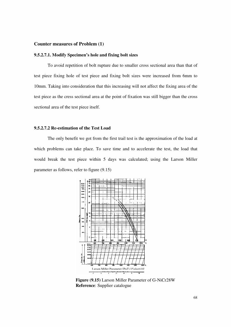
9.5.2.7.2 Re-estimation of the Test Load

The only benefit we got from the first trail test is the approximation of the load at

which problems can take place. To save time and to accelerate the test, the load that

would break the test piece within 5 days was calculated; using the Larson Miller

parameter as follows, refer to figure (9.15)

Larson Miller Parameter [P=T (15+logt)10-

Figure (9.15) Larson Miller Parameter of G-NiCr28W

Reference: Supplier catalogue

69

P= T (K) (15 + log t)10-3

P =1273 (15 + 2.079) 10-3

P = 21.74

From the graph the stress would be approximately 27 N/mm2 so the load would be 1944

N and according to the machine ratio 77.76 N would be loaded on the loading plate.

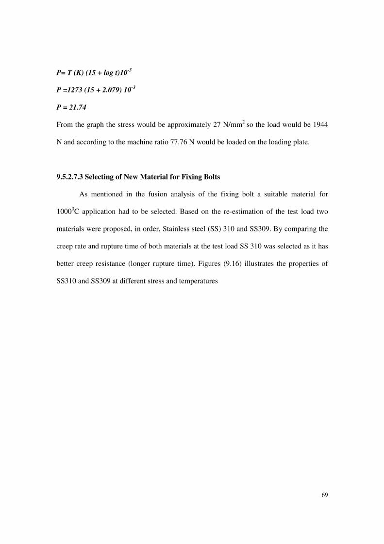
9.5.2.7.3 Selecting of New Material for Fixing Bolts

As mentioned in the fusion analysis of the fixing bolt a suitable material for

10000C application had to be selected. Based on the re-estimation of the test load two

materials were proposed, in order, Stainless steel (SS) 310 and SS309. By comparing the

creep rate and rupture time of both materials at the test load SS 310 was selected as it has

better creep resistance (longer rupture time). Figures (9.16) illustrates the properties of

SS310 and SS309 at different stress and temperatures

70

For further simplification and facilitate machining, fixation was changed from bolts to

pins

9.5.2.7.4 Replacing screws of the extensometer

Screws of the extensometer had to be replaced by another ones that can resist high

temperature applications. There was no stock of stainless steel screws at machine shop

and only SS316 screws were only available in the market. SS316 has inferior properties

at elevated temperature compared with SS310. However it has been used because the

Figure (9.16) Properties of SS309 and 310 at elevated temperatures.

Reference: NiDI Publication No.2980

71

screws were no subjected to any stress, their main functions are to hold the extensometer

legs at its position.

9.5.2.8 Furnace Re-set up and Test piece Heating up

Light up the furnace re-started after taking all the counter measures related to

problem (1). Heating up regime was the same as the first trial test.

9.5.2.9 Loading the Test piece

During heating up of the test piece just only 7 Newton load (10% of the test load)

was loaded on the loading plate for keeping the machine parts straight. 77.76 Newton was

loaded after heating up and socking of the test piece

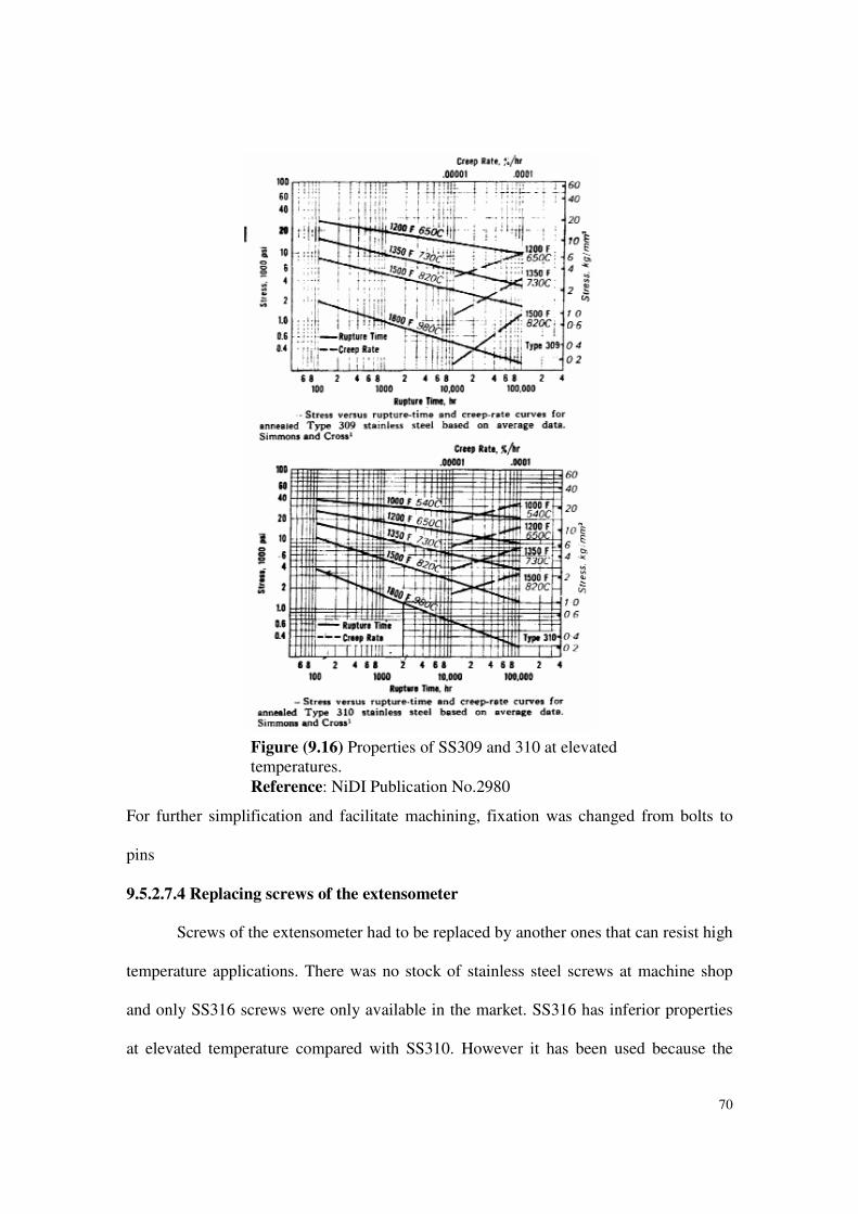
9.5.2.10 Encountering of Problem (2)

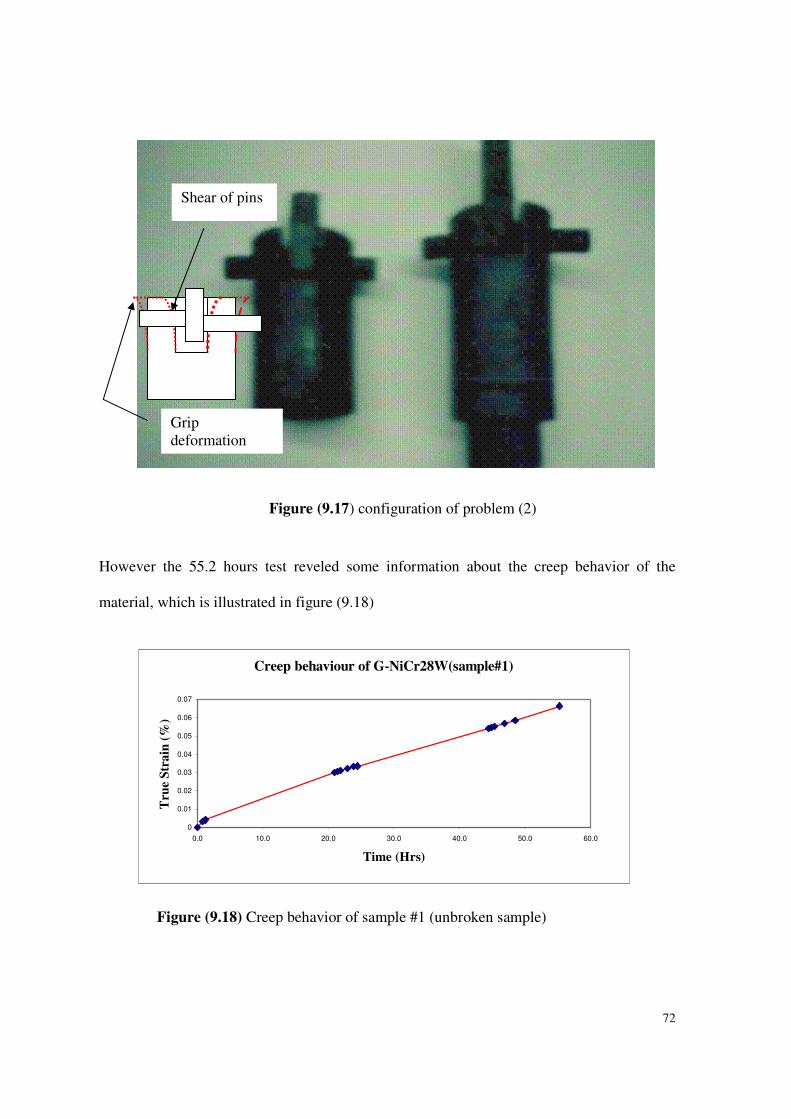
After 55.2 hours problem No (2) was encountered which is illustrated in figure

(9.17) and summarized as follows:

1. Shearing of the new fixing pins

2. Deformation of the grips

72

However the 55.2 hours test reveled some information about the creep behavior of the

material, which is illustrated in figure (9.18)

Grip deformation

Shear of pins

Figure (9.17) configuration of problem (2)

Creep behaviour of G-NiCr28W(sample#1)

0

0.01

0.02

0.03

0.04

0.05

0.06

0.07

0.0 10.0 20.0 30.0 40.0 50.0 60.0

Time (Hrs)

Tru

e S

tra

in (

%)

Figure (9.18) Creep behavior of sample #1 (unbroken sample)

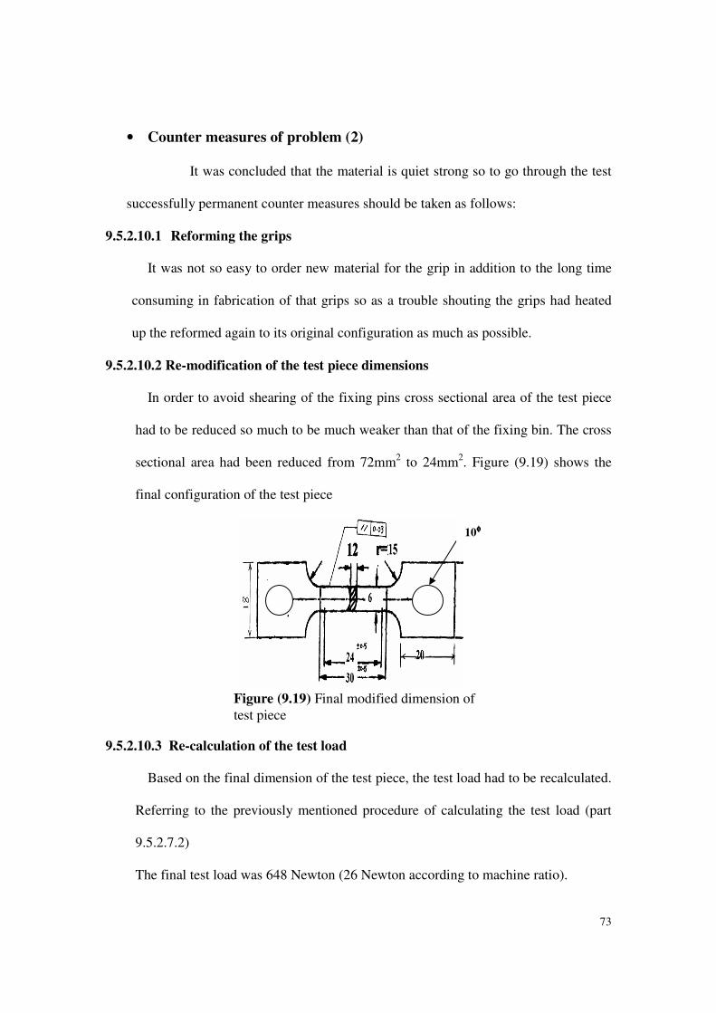
73

• Counter measures of problem (2)

It was concluded that the material is quiet strong so to go through the test

successfully permanent counter measures should be taken as follows:

9.5.2.10.1 Reforming the grips

It was not so easy to order new material for the grip in addition to the long time

consuming in fabrication of that grips so as a trouble shouting the grips had heated

up the reformed again to its original configuration as much as possible.

9.5.2.10.2 Re-modification of the test piece dimensions

In order to avoid shearing of the fixing pins cross sectional area of the test piece

had to be reduced so much to be much weaker than that of the fixing bin. The cross

sectional area had been reduced from 72mm2 to 24mm2. Figure (9.19) shows the

final configuration of the test piece

9.5.2.10.3 Re-calculation of the test load

Based on the final dimension of the test piece, the test load had to be recalculated.

Referring to the previously mentioned procedure of calculating the test load (part

9.5.2.7.2)

The final test load was 648 Newton (26 Newton according to machine ratio).

Figure (9.19) Final modified dimension of test piece

10φφφφ

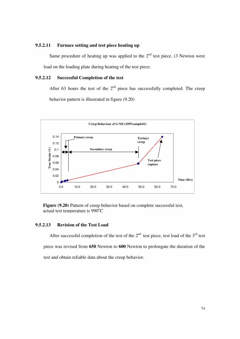
74

9.5.2.11 Furnace setting and test piece heating up

Same procedure of heating up was applied to the 2nd test piece. (3 Newton were

load on the loading plate during heating of the test piece.

9.5.2.12 Successful Completion of the test

After 63 hours the test of the 2nd piece has successfully completed. The creep

behavior pattern is illustrated in figure (9.20)

Creep Behaviour of G-NiCr28W(sample#2)

0

0.02

0.04

0.06

0.08

0.1

0.12

0.14

0.0 10.0 20.0 30.0 40.0 50.0 60.0 70.0

Time (Hrs)

Tru

e S

train

(%

)

Secondary creep

Primary creep

Test piece

rupture

9.5.2.13 Revision of the Test Load

After successful completion of the test of the 2nd test piece, test load of the 3rd test

piece was revised from 650 Newton to 600 Newton to prolongate the duration of the

test and obtain reliable data about the creep behavior.

Figure (9.20) Pattern of creep behavior based on complete successful test, actual test temperature is 990oC

Tertiary

creep

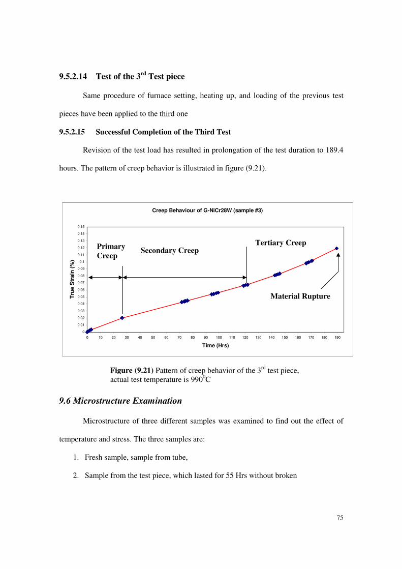
75

9.5.2.14 Test of the 3rd

Test piece

Same procedure of furnace setting, heating up, and loading of the previous test

pieces have been applied to the third one

9.5.2.15 Successful Completion of the Third Test

Revision of the test load has resulted in prolongation of the test duration to 189.4

hours. The pattern of creep behavior is illustrated in figure (9.21).

Creep Behaviour of G-NiCr28W (sample #3)

0

0.01

0.02

0.03

0.04

0.05

0.06

0.07

0.08

0.09

0.1

0.11

0.12

0.13

0.14

0.15

0 10 20 30 40 50 60 70 80 90 100 110 120 130 140 150 160 170 180 190

Time (Hrs)

Tru

e S

train

(%

)

9.6 Microstructure Examination

Microstructure of three different samples was examined to find out the effect of

temperature and stress. The three samples are:

1. Fresh sample, sample from tube,

2. Sample from the test piece, which lasted for 55 Hrs without broken

Secondary Creep Primary

Creep

Material Rupture

Figure (9.21) Pattern of creep behavior of the 3rd test piece, actual test temperature is 9900C

Tertiary Creep

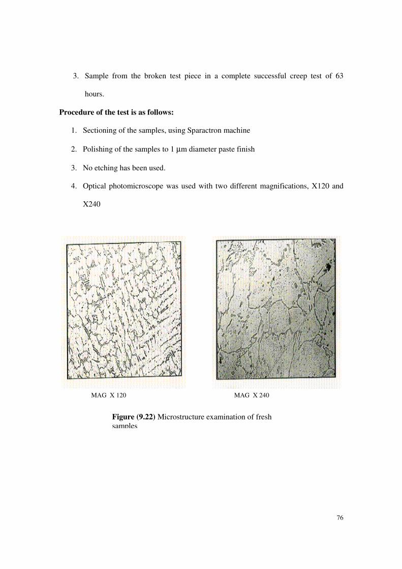
76

3. Sample from the broken test piece in a complete successful creep test of 63

hours.

Procedure of the test is as follows:

1. Sectioning of the samples, using Sparactron machine

2. Polishing of the samples to 1 µm diameter paste finish

3. No etching has been used.

4. Optical photomicroscope was used with two different magnifications, X120 and

X240

Figure (9.22) Microstructure examination of fresh samples

MAG X 120 MAG X 240

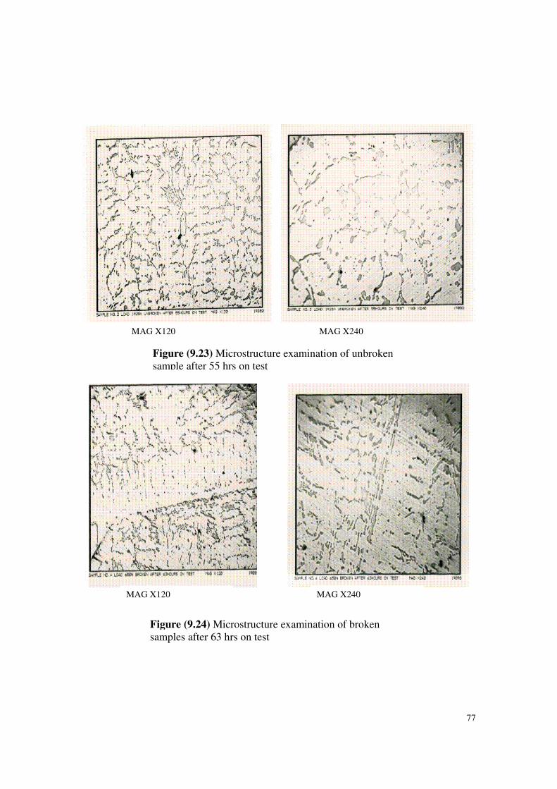
77

Figure (9.23) Microstructure examination of unbroken sample after 55 hrs on test

Figure (9.24) Microstructure examination of broken samples after 63 hrs on test

MAG X120 MAG X240

MAG X120 MAG X240

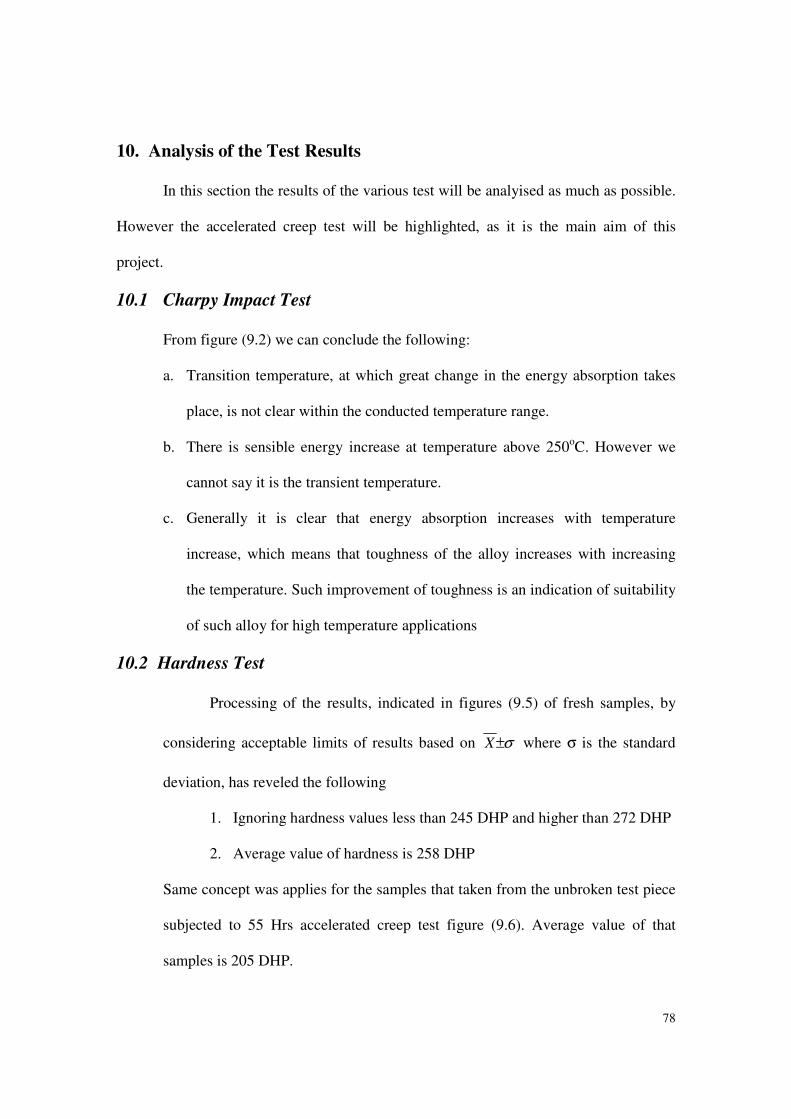
78

10. Analysis of the Test Results

In this section the results of the various test will be analyised as much as possible.

However the accelerated creep test will be highlighted, as it is the main aim of this

project.

10.1 Charpy Impact Test

From figure (9.2) we can conclude the following:

a. Transition temperature, at which great change in the energy absorption takes

place, is not clear within the conducted temperature range.

b. There is sensible energy increase at temperature above 250oC. However we

cannot say it is the transient temperature.

c. Generally it is clear that energy absorption increases with temperature

increase, which means that toughness of the alloy increases with increasing

the temperature. Such improvement of toughness is an indication of suitability

of such alloy for high temperature applications

10.2 Hardness Test

Processing of the results, indicated in figures (9.5) of fresh samples, by

considering acceptable limits of results based on σ±X where σ is the standard

deviation, has reveled the following

1. Ignoring hardness values less than 245 DHP and higher than 272 DHP

2. Average value of hardness is 258 DHP

Same concept was applies for the samples that taken from the unbroken test piece

subjected to 55 Hrs accelerated creep test figure (9.6). Average value of that

samples is 205 DHP.

79

It is clear that hardness decreases after subjecting the test piece to heat for

sometimes. Decreasing the hardness increases the toughness of the alloy and

hence the resistance of the alloy fore crack propagation. This is another prove of

the suitability of such alloy for high temperature applications and underlines the

result of charpy impact test, in the way that when the alloy subjects to high

temperature its hardness decreases and accordingly the strength. Decreasing the

strength improve the toughness.

10.3 Tensile Test

The only property needed from that test was the tensile strength of the alloy in

question. Results of the test as indicated in table (9.1) shows some variation of maximum

load to break the test piece. By ignoring the shaded values, which are the lowest and

highest values of either load or extension we obtain an average value of max. Load as

2628 Newton.

Thus

Tensile strength = Max Load/ original cross sectional area

= 2628/6 = 438 N/mm2

This figure is around the specification of that alloy which mentioned in table (8.2)

10.4 Accelerated Creep Test;

The result of the accelerated creep test will be analyised from the following

viewpoints:

• Creep Curve Pattern

• Creep rate

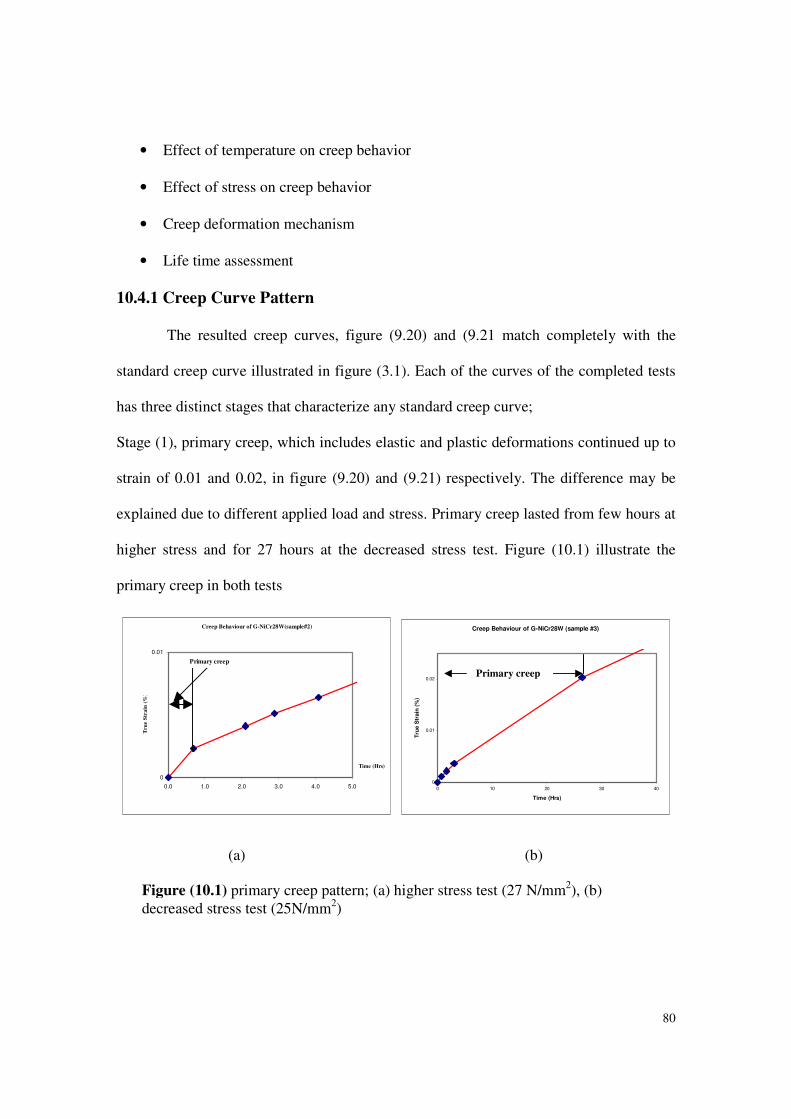
80

• Effect of temperature on creep behavior

• Effect of stress on creep behavior

• Creep deformation mechanism

• Life time assessment

10.4.1 Creep Curve Pattern

The resulted creep curves, figure (9.20) and (9.21 match completely with the

standard creep curve illustrated in figure (3.1). Each of the curves of the completed tests

has three distinct stages that characterize any standard creep curve;

Stage (1), primary creep, which includes elastic and plastic deformations continued up to

strain of 0.01 and 0.02, in figure (9.20) and (9.21) respectively. The difference may be

explained due to different applied load and stress. Primary creep lasted from few hours at

higher stress and for 27 hours at the decreased stress test. Figure (10.1) illustrate the

primary creep in both tests

Creep Behaviour of G-NiCr28W(sample#2)

0

0.01

0.0 1.0 2.0 3.0 4.0 5.0

Time (Hrs)

Tru

e S

tra

in (

%)

Primary creep

Creep Behaviour of G-NiCr28W (sample #3)

0

0.01

0.02

0 10 20 30 40

Time (Hrs)

Tru

e S

tra

in (

%)

Primary creep

(a) (b)

Figure (10.1) primary creep pattern; (a) higher stress test (27 N/mm2), (b) decreased stress test (25N/mm2)

81

10.4.2 Creep rate

Stage (2) in both curves of figure (9.20) and (9.21) lasted for 44.3 and 95.5 hours

respectively. The slop of the secondary creep represents the creep rate, which is as

follows:

��∃∃∃∃

s = 0.0012% /Hr for the higher stress test (27 N/mm2), figure (9.20)

��∃∃∃∃

s = 0.000494% /Hr for the decreased stress test (25 N/mm2), figure (9.21)

This result matches with the equation (3.2) and (3.4) in which ��∃∃∃∃

s α σσσσn

10.4.3 Effect of Temperature on creep behavior

In fact there was no chance to examine the effect of different temperature on the

pattern of creep behavior. The test has been conduct at only one temperature 980 0C

deg10± .

10.4.4 Effect of stress on creep behavior

By comparing the curves of figures (9.20) and (9.21) we can see clearly that when

the load decreased from 650 Newton (27 N/mm2) to 600 Newton (25 N/mm2) the creep

rate of secondary creep decreased to more than a half of its value and hence the

secondary creep duration increased to more than a double. Meanwhile the fracture time

was three times of the higher stress test.

10.4.5 Creep mechanism

To classify the creep mechanism according to the simplified creep deformation

map, figure (5.1) we have to determine the shear modulus of the alloy.

Shear modulus of the main components is illustrated in table (10.1)

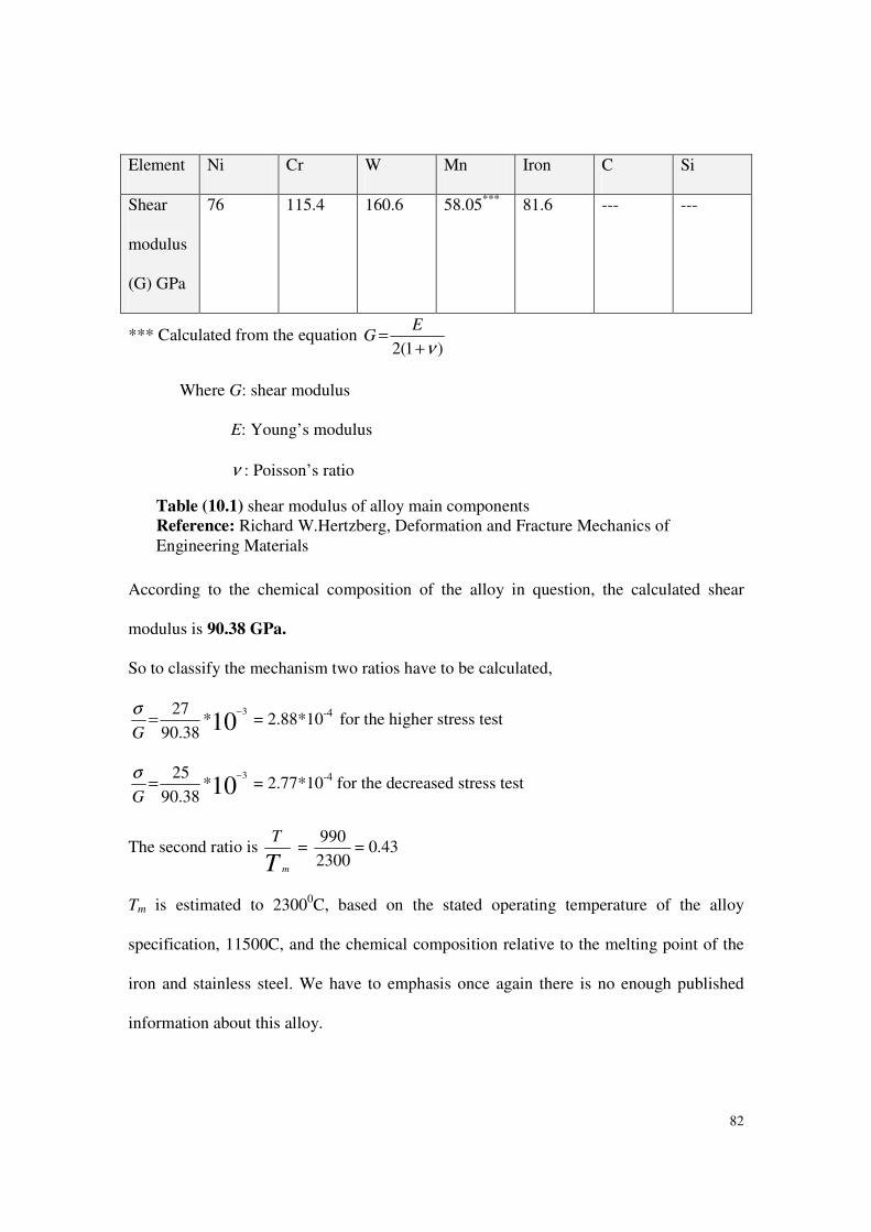
82

Element Ni Cr W Mn Iron C Si

Shear

modulus

(G) GPa

76 115.4 160.6 58.05*** 81.6 --- ---

*** Calculated from the equation )1(2 ν+

=E

G

Where G: shear modulus

E: Young’s modulus

ν : Poisson’s ratio

According to the chemical composition of the alloy in question, the calculated shear

modulus is 90.38 GPa.

So to classify the mechanism two ratios have to be calculated,

103

*38.90

27 −=

G

σ = 2.88*10-4 for the higher stress test

103

*38.90

25 −=

G

σ = 2.77*10-4 for the decreased stress test

The second ratio is T m

T =

2300

990= 0.43

Tm is estimated to 23000C, based on the stated operating temperature of the alloy

specification, 11500C, and the chemical composition relative to the melting point of the

iron and stainless steel. We have to emphasis once again there is no enough published

information about this alloy.

Table (10.1) shear modulus of alloy main components Reference: Richard W.Hertzberg, Deformation and Fracture Mechanics of Engineering Materials

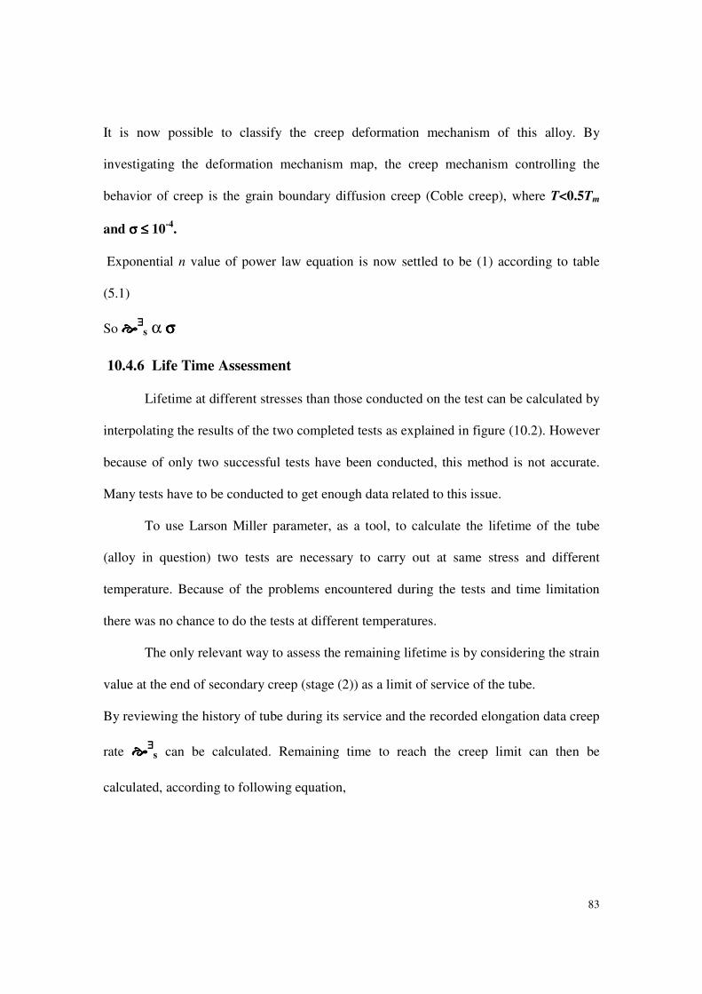
83

It is now possible to classify the creep deformation mechanism of this alloy. By

investigating the deformation mechanism map, the creep mechanism controlling the

behavior of creep is the grain boundary diffusion creep (Coble creep), where T<0.5Tm

and σσσσ ≤≤≤≤ 10-4

.

Exponential n value of power law equation is now settled to be (1) according to table

(5.1)

So ��∃∃∃∃

s α σσσσ

10.4.6 Life Time Assessment

Lifetime at different stresses than those conducted on the test can be calculated by

interpolating the results of the two completed tests as explained in figure (10.2). However

because of only two successful tests have been conducted, this method is not accurate.

Many tests have to be conducted to get enough data related to this issue.

To use Larson Miller parameter, as a tool, to calculate the lifetime of the tube

(alloy in question) two tests are necessary to carry out at same stress and different

temperature. Because of the problems encountered during the tests and time limitation

there was no chance to do the tests at different temperatures.

The only relevant way to assess the remaining lifetime is by considering the strain

value at the end of secondary creep (stage (2)) as a limit of service of the tube.

By reviewing the history of tube during its service and the recorded elongation data creep

rate ��∃∃∃∃

s can be calculated. Remaining time to reach the creep limit can then be

calculated, according to following equation,

84

Remaining lifetime (t) = )(

)(0675.0.

ε

ε

sratecreepactual

valuestrainpresent−

Stress Vs Life time

24

25

26

27

28

0 50 100 150 200

Time (Hrs)

Str

ess

(N/m

m2)

10.5 Microstructure Test

By reviewing the microstructure photos, figure (9.22) we observe the following,

1. The network is dendritic structure.

2. Grain and grain boundaries are seen

3. Some traces of carbide are exist

Comparing the structure of the fresh sample and the other samples we can conclude

the following

1. When the alloy subjected to creep test, grain boundaries started disappearing,

due to deformation as indicated in figure (9.23)

2. Complete part of grain boundary disappeared as indicated in figure (9.24)

3. Disappearing of grain boundary may be regarded as the initiation of

component fracture.

Figure (10.2) Relation between stress and lifetime of the two accelerated creep tests.

X= 1768.05-63.15 Y

85

11. Conclusion

From the previous sections, test results and analysis, we can conclude the

following points

1. Creep behavior of G-NiCr28W is a standard pattern of creep curve

2. The Creep rate depends on the applied stress typical rate according to the test

stress is 0.0012 %/Hr and 0.000494 %/Hr at 27 N/mm2 and 25 N/mm2

respectively.

3. Strain of 0.0675% is limit determines the lifetime of the tube

4. Lifetime regression equation X = 1768.05 – 63.15 Y can be used to calculate the

lifetime in the stress range of 25 to 27 N/mm2.

5. Based on strain limit of 0.0675%, remaining lifetime of the tubes is calculated

using the equation (t) = )(

)(0675.0.

ε

ε

sratecreepactual

valuestrainpresent−.

6. Grain boundary diffusion creep, Coble creep, controls the creep behavior of G-

NiCr28W alloy, in the operating temperature and stress regime.

7. Tube toughness resistance to crack propagation, increases with increasing the

operating temperature.

8. Tube hardness decreases with temperature increases.

86

12. Future Plan and Recommendations

For deep investigation of the creep behavior of G-NiCr28W tube the following

are will consider as a future plan and recommendation for the company as well,

1. Study the effect of temperature on the creep behavior pattern, at constant

stress.

2. Conduct accelerated creep test at different temperature to calculated Larson

Miller parameter, for the purpose of establishing general equation for

remaining lifetime.

3. Study the creep failure mechanism to find put a way to improve the lifetime.

4. Study the recorded data about the elongation tube during its service life to

determine the strain rate and estimation of the remaining lifetime.

5. Due to possibility of changing the operating condition accelerated creep test is

recommended to carry out at certain times, during the entire service of the

tube, to confirm the remaining lifetime.

87

13. References

1. Marc Andre and Krishan Kumar Chawla, “Mechanical Behavior of Materials”

2. R.W.Evans and B.Wilshire, “Introduction to Creep”

3. Junhui Li, “Failure Mechanism Models for Creep and Creep Rupture”, IEEE

Transactions on Reliability, Vol.42, NO.3, 1993 Septemper

4. B.J. Cane et al, “Creep Life assessment Methods”, Journal of Strain Analysis, Vol.

29, NO. 3,1994

5. Shiqiang Deng, “High Temperature Creep Behavior of Single Crystal Oxides”,

Journal of Materials Science 31 (1996) 6077-6083

6. G.A.Webster, “Fracture Mechanics in the Creep Range”, Journal of Strain Analysis

Vol. 29, No.3, 1994

7. David M. Owen et al, “Low Stress Creep Behavior an Examination of Nabarro-

Herring and Happer- Dorn Creep”, Material Science and Engineering A216(1996)

20-29

8. Y.Kaizumi et al, “Creep Life Extension of a Single Crystal Superalloy”,

http://www/nrim.go.jp:8080/open/usr/harada/documents/990225m.html

9. Richard W.Hertzberg, “ Deformation and Fracture Mechanics of Engineering

Materials”

10. Sixth International Confernece, 15-17 April,1996, “ Creep and Fatigue”

11. J.Bresser, “ Creep and Fatigue in High Temperature Alloys”

88

12. Iain Finnie and William R.Heller, “ Creep of Engineering Materials”

13. A.J.Fenner, “ Mechanical Testing of Material

14. Nickel Development Institute (NiDI), “Austenitic Chromium- Nickel, Stainless Steel

Engineering Properties at Elevated Temperature”, Publication No. 2980

15. Nickel Development Institute (NiDI), “ Properties of Some Metals and Alloys”,

Publication No. 297

16. Supplier Catalogue

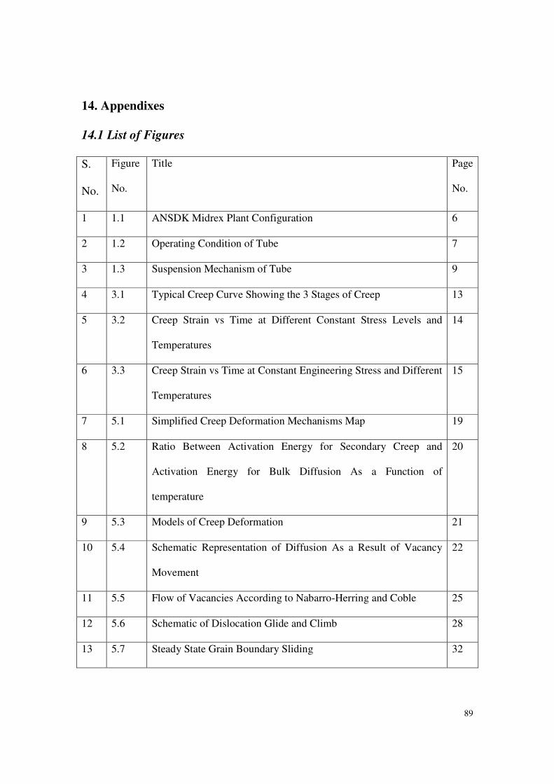
89

14. Appendixes

14.1 List of Figures

S.

No.

Figure

No.

Title Page

No.

1 1.1 ANSDK Midrex Plant Configuration 6

2 1.2 Operating Condition of Tube 7

3 1.3 Suspension Mechanism of Tube 9

4 3.1 Typical Creep Curve Showing the 3 Stages of Creep 13

5 3.2 Creep Strain vs Time at Different Constant Stress Levels and

Temperatures

14

6 3.3 Creep Strain vs Time at Constant Engineering Stress and Different

Temperatures

15

7 5.1 Simplified Creep Deformation Mechanisms Map 19

8 5.2 Ratio Between Activation Energy for Secondary Creep and

Activation Energy for Bulk Diffusion As a Function of

temperature

20

9 5.3 Models of Creep Deformation 21

10 5.4 Schematic Representation of Diffusion As a Result of Vacancy

Movement

22

11 5.5 Flow of Vacancies According to Nabarro-Herring and Coble 25

12 5.6 Schematic of Dislocation Glide and Climb 28

13 5.7 Steady State Grain Boundary Sliding 32

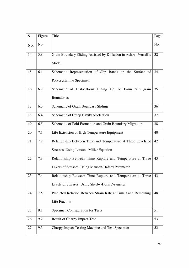
90

S.

No.

Figure

No.

Title Page

No.

14 5.8 Grain Boundary Sliding Assisted by Diffusion in Ashby- Verrall’s

Model

32

15 6.1 Schematic Representation of Slip Bands on the Surface of

Polycrystalline Specimen

34

16 6.2 Schematic of Dislocations Lining Up To Form Sub grain

Boundaries

35

17 6.3 Schematic of Grain Boundary Sliding 36

18 6.4 Schematic of Creep Cavity Nucleation 37

19 6.5 Schematic of Fold Formation and Grain Boundary Migration 38

20 7.1 Life Extension of High Temperature Equipment 40

21 7.2 Relationship Between Time and Temperature at Three Levels of

Stresses, Using Larson –Miller Equation

42

22 7.3 Relationship Between Time Rupture and Temperature at Three

Levels of Stresses, Using Manson-Haferd Parameter

43

23 7.4 Relationship Between Time Rupture and Temperature at Three

Levels of Stresses, Using Sherby-Dorn Parameter

43

24 7.5 Predicted Relation Between Strain Rate at Time t and Remaining

Life Fraction

48

25 9.1 Specimen Configuration for Tests 51

26 9.2 Result of Charpy Impact Test 53

27 9.3 Charpy Impact Testing Machine and Test Specimen 53

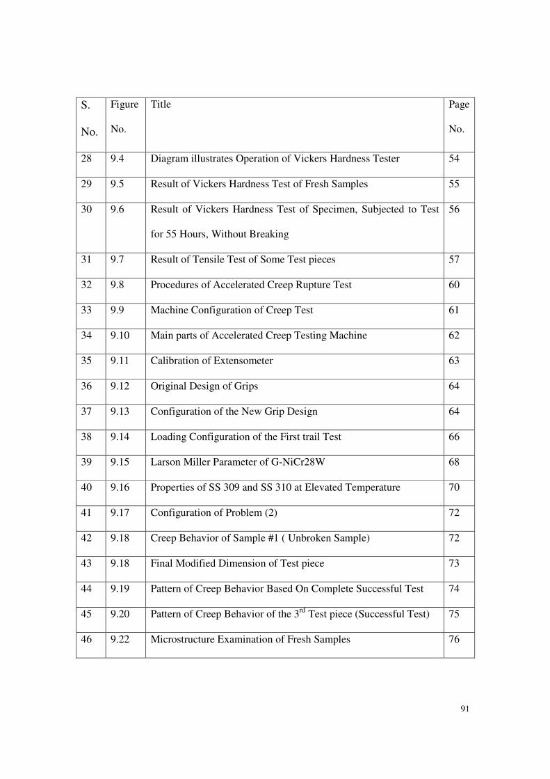
91

S.

No.

Figure

No.

Title Page

No.

28 9.4 Diagram illustrates Operation of Vickers Hardness Tester 54

29 9.5 Result of Vickers Hardness Test of Fresh Samples 55

30 9.6 Result of Vickers Hardness Test of Specimen, Subjected to Test

for 55 Hours, Without Breaking

56

31 9.7 Result of Tensile Test of Some Test pieces 57

32 9.8 Procedures of Accelerated Creep Rupture Test 60

33 9.9 Machine Configuration of Creep Test 61

34 9.10 Main parts of Accelerated Creep Testing Machine 62

35 9.11 Calibration of Extensometer 63

36 9.12 Original Design of Grips 64

37 9.13 Configuration of the New Grip Design 64

38 9.14 Loading Configuration of the First trail Test 66

39 9.15 Larson Miller Parameter of G-NiCr28W 68

40 9.16 Properties of SS 309 and SS 310 at Elevated Temperature 70

41 9.17 Configuration of Problem (2) 72

42 9.18 Creep Behavior of Sample #1 ( Unbroken Sample) 72

43 9.18 Final Modified Dimension of Test piece 73

44 9.19 Pattern of Creep Behavior Based On Complete Successful Test 74

45 9.20 Pattern of Creep Behavior of the 3rd Test piece (Successful Test) 75

46 9.22 Microstructure Examination of Fresh Samples 76

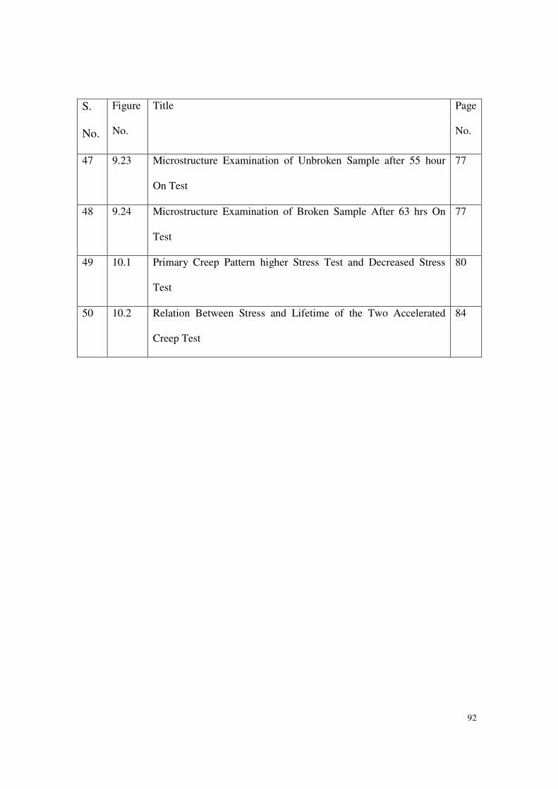
92

S.

No.

Figure

No.

Title Page

No.

47 9.23 Microstructure Examination of Unbroken Sample after 55 hour

On Test

77

48 9.24 Microstructure Examination of Broken Sample After 63 hrs On

Test

77

49 10.1 Primary Creep Pattern higher Stress Test and Decreased Stress

Test

80

50 10.2 Relation Between Stress and Lifetime of the Two Accelerated

Creep Test

84

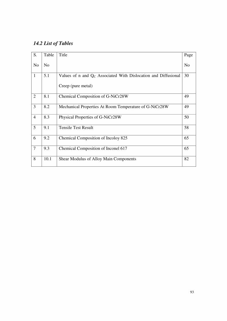
93

14.2 List of Tables

S.

No

Table

No

Title Page

No

1 5.1 Values of n and QC Associated With Dislocation and Diffusional

Creep (pure metal)

30

2 8.1 Chemical Composition of G-NiCr28W 49

3 8.2 Mechanical Properties At Room Temperature of G-NiCr28W 49

4 8.3 Physical Properties of G-NiCr28W 50

5 9.1 Tensile Test Result 58

6 9.2 Chemical Composition of Incoloy 825 65

7 9.3 Chemical Composition of Inconel 617 65

8 10.1 Shear Modulus of Alloy Main Components 82

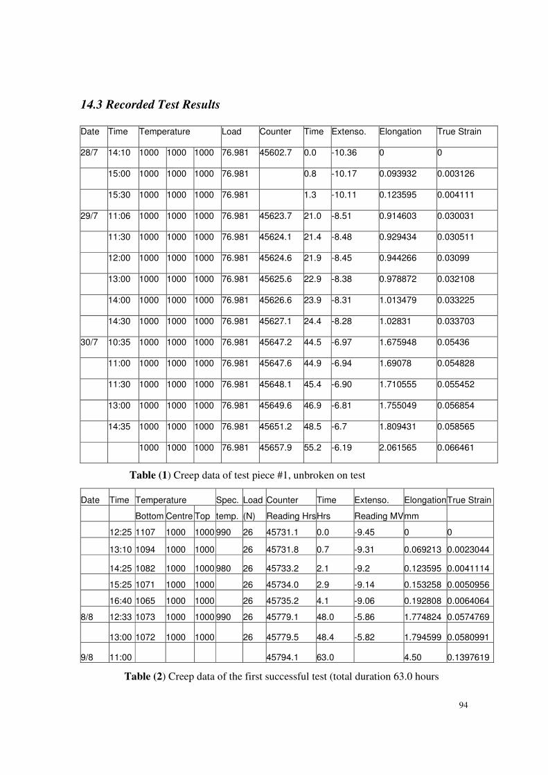
94

14.3 Recorded Test Results

Date Time Temperature Load Counter Time Extenso. Elongation True Strain

28/7 14:10 1000 1000 1000 76.981 45602.7 0.0 -10.36 0 0

15:00 1000 1000 1000 76.981 0.8 -10.17 0.093932 0.003126

15:30 1000 1000 1000 76.981 1.3 -10.11 0.123595 0.004111

29/7 11:06 1000 1000 1000 76.981 45623.7 21.0 -8.51 0.914603 0.030031

11:30 1000 1000 1000 76.981 45624.1 21.4 -8.48 0.929434 0.030511

12:00 1000 1000 1000 76.981 45624.6 21.9 -8.45 0.944266 0.03099

13:00 1000 1000 1000 76.981 45625.6 22.9 -8.38 0.978872 0.032108

14:00 1000 1000 1000 76.981 45626.6 23.9 -8.31 1.013479 0.033225

14:30 1000 1000 1000 76.981 45627.1 24.4 -8.28 1.02831 0.033703

30/7 10:35 1000 1000 1000 76.981 45647.2 44.5 -6.97 1.675948 0.05436

11:00 1000 1000 1000 76.981 45647.6 44.9 -6.94 1.69078 0.054828

11:30 1000 1000 1000 76.981 45648.1 45.4 -6.90 1.710555 0.055452

13:00 1000 1000 1000 76.981 45649.6 46.9 -6.81 1.755049 0.056854

14:35 1000 1000 1000 76.981 45651.2 48.5 -6.7 1.809431 0.058565

1000 1000 1000 76.981 45657.9 55.2 -6.19 2.061565 0.066461

Date Time Temperature Spec. Load Counter Time Extenso. Elongation True Strain

Bottom Centre Top temp. (N) Reading HrsHrs Reading MV mm

12:25 1107 1000 1000 990 26 45731.1 0.0 -9.45 0 0

13:10 1094 1000 1000 26 45731.8 0.7 -9.31 0.069213 0.0023044

14:25 1082 1000 1000 980 26 45733.2 2.1 -9.2 0.123595 0.0041114

15:25 1071 1000 1000 26 45734.0 2.9 -9.14 0.153258 0.0050956

16:40 1065 1000 1000 26 45735.2 4.1 -9.06 0.192808 0.0064064

8/8 12:33 1073 1000 1000 990 26 45779.1 48.0 -5.86 1.774824 0.0574769

13:00 1072 1000 1000 26 45779.5 48.4 -5.82 1.794599 0.0580991

9/8 11:00 45794.1 63.0 4.50 0.1397619

Table (1) Creep data of test piece #1, unbroken on test

Table (2) Creep data of the first successful test (total duration 63.0 hours

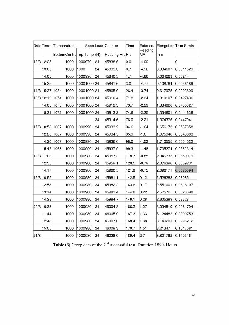
95

Date Time Temperature Spec.Load Counter Time Extenso. Elongation True Strain

Bottom CentreTop temp. (N) Reading HrsHrs Reading MV mm

13/8 12:25 1000 1000 970 24 45838.6 0.0 -4.99 0 0

13:05 1000 1000 24 45839.3 0.7 -4.92 0.034607 0.0011529

14:05 1000 1000 990 24 45840.3 1.7 -4.86 0.064269 0.00214

15:25 1000 1000 1000 24 45841.6 3.0 -4.77 0.108764 0.0036189

14/8 15:37 1084 1000 1000 1000 24 45865.0 26.4 -3.74 0.617975 0.0203899

16/8 12:10 1074 1000 1000 1000 24 45910.4 71.8 -2.34 1.310107 0.0427436

14:05 1075 1000 1000 1000 24 45912.3 73.7 -2.29 1.334826 0.0435327

15:21 1072 1000 1000 1000 24 45913.2 74.6 -2.25 1.354601 0.0441636

24 45914.6 76.0 -2.21 1.374376 0.0447941

17/8 10:58 1067 1000 1000 990 24 45933.2 94.6 -1.64 1.656173 0.0537358

12:20 1067 1000 1000 990 24 45934.5 95.9 -1.6 1.675948 0.0543603

14:20 1069 1000 1000 990 24 45936.6 98.0 -1.53 1.710555 0.0554522

15:42 1068 1000 1000 990 24 45937.9 99.3 -1.48 1.735274 0.0562314

18/8 11:03 1000 1000 980 24 45957.3 118.7 -0.85 2.046733 0.0659979

12:55 1000 1000 980 24 45959.1 120.5 -0.79 2.076396 0.0669231

14:17 1000 1000 980 24 45960.5 121.9 -0.75 2.096171 0.0675394

19/8 10:55 1000 1000 980 24 45981.1 142.5 0.12 2.526282 0.0808511

12:58 1000 1000 980 24 45982.2 143.6 0.17 2.551001 0.0816107

13:14 1000 1000 980 24 45983.4 144.8 0.22 2.57572 0.0823698

14:28 1000 1000 980 24 45984.7 146.1 0.28 2.605383 0.08328

20/8 10:35 1000 1000 980 24 46004.8 166.2 1.27 3.094819 0.0981794

11:44 1000 1000 980 24 46005.9 167.3 1.33 3.124482 0.0990753

12:48 1000 1000 980 24 46007.0 168.4 1.38 3.149201 0.0998212

15:05 1000 1000 980 24 46009.3 170.7 1.51 3.21347 0.1017581

21/8 1000 1000 980 24 46028.0 189.4 2.7 3.801782 0.1193161

Table (3) Creep data of the 2nd successful test. Duration 189.4 Hours

microsoft word - creep behaviour of reformer tubes

Documents