microphone suppression of air-noise … suppression of air-noise on geophones----- a thesis...

MICROPHONE SUPPRESSION OF AIR-NOISE ON GEOPHONES

----------------------------------------------------

A Thesis

Presented to

the Faculty of the Department of Earth and Atmospheric Sciences

University of Houston

----------------------------------------------------

In Partial Fulfillment

of the Requirements for the Degree

Master of Science

----------------------------------------------------

By

Nathanael Mark Babcock

August 2012

ii


__________________________________________


APPROVED:

__________________________________________

Dr. Robert Stewart, Chairman

__________________________________________

Dr. Christopher Liner

__________________________________________

Dr. Stephen Danbom

__________________________________________

Dean, College of Natural Sciences and Mathematics

iii

ACKNOWLEDGEMENTS

I would like to thank Ady Geda, who helped me acquire all of my seismic data, and Li

Chang, for assistance and expertise in the field and helping me with software. None

of my 350 data sets would be possible without their assistance. I greatly appreciate

Dr. Stewart, for the idea and foundation of my project, as well as everyone at the

University of Calgary who previously worked on this topic. Last, but not least, I

would like to thank my family for their overwhelming moral support and guidance.

iv


----------------------------------------------------

An Abstract of a Thesis

Presented to

the Faculty of the Department of Earth and Atmospheric Sciences

University of Houston

----------------------------------------------------

In Partial Fulfillment

of the Requirements for the Degree

Master of Science

----------------------------------------------------

By


August 2012

v

ABSTRACT

Air-noise in seismic records creates a loss in signal quality, reducing seismic image

clarity. A microphone may be used to estimate and remove air-noise in seismic

records. This thesis covers the characterization of air-noise on a prototype 4-

Component geophone (3-C geophone plus microphone), as well as the development

of two air-noise removal filters. Vibration-isolated, noise characterization

experiments were performed to determine the 4-C geophone’s directional and

frequency dependent response to air-noise. Sensor placement within the geophone

appeared to affect each geophone component’s directional response; showing

increased sensitivity to sounds from the same side the sensor was mounted. In

addition, a walk-away seismic survey was performed to determine the effect of

distance on geophone air-noise. Peak amplitude decay rates differed from the

theoretical 1/R, R representing total distance. The microphone and inline geophone

decayed at 1/R1.4, the crossline component at 1/R1.15, and the vertical component at

1/R1.81. These results indicate a loss of energy to heat through air-ground

interactions. Results from the noise characterization tests were used to develop two

air-noise filters; a real-time filter, which could remove air-noise from geophone

signals before they are recorded; and a post-acquisition filter, which could be used

to more precisely remove air-noise. Both filters were effective at reducing air-noise,

up to 21 dB reduction for near offsets. However, the real-time filter affected seismic

data due to microphone recorded seismic events.

vi

CONTENTS

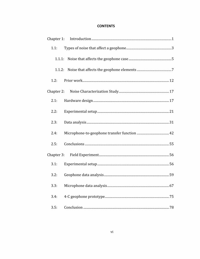
Chapter 1: Introduction ................................................................................................. 1

1.1: Types of noise that affect a geophone ....................................................... 3

1.1.1: Noise that affects the geophone case .................................................... 5

1.1.2: Noise that affects the geophone elements .......................................... 7

1.2: Prior work......................................................................................................... 12

Chapter 2: Noise Characterization Study ............................................................. 17

2.1: Hardware design ............................................................................................ 17

2.2: Experimental setup ....................................................................................... 21

2.3: Data analysis .................................................................................................... 31

2.4: Microphone-to-geophone transfer function ....................................... 42

2.5: Conclusions ...................................................................................................... 55

Chapter 3: Field Experiment ..................................................................................... 56

3.1: Experimental setup ....................................................................................... 56

3.2: Geophone data analysis ............................................................................... 59

3.3: Microphone data analysis ........................................................................... 67

3.4: 4-C geophone prototype.............................................................................. 75

3.5: Conclusion ........................................................................................................ 78

vii

Chapter 4: Noise-Cancelling Filter .......................................................................... 79

4.1: Filter design ..................................................................................................... 79

4.2: Filter results ..................................................................................................... 87

4.2.1: Vertical component ................................................................................... 88

4.2.2: Crossline component ................................................................................ 92

4.2.3: Inline component ....................................................................................... 95

4.3: Conclusion ........................................................................................................ 98

Chapter 5: Discussion and Conclusions ............................................................. 100

Appendix A: Real-time Air-noise Filter ................................................................. 105

Appendix B: Patents ..................................................................................................... 113

References ................................................................................................................................... 116

viii

LIST OF FIGURES

Figure 1.1: Left: Diagram of a MEMS accelerometer (Hons and Stewart,

2007). As ground accelerations displace the seismic mass there is a

capacitance change at the top and bottom electrodes. Right: A cutout

analog geophone. The geophone case moves about the seismic mass

(copper coils) when subjected to ground motion. The voltage created

by the coil is proportional to ground velocity. ........................................................... 4

Figure 1.2: Left: Power spectral density (PSD) comparison of wind noise

(lower line) and M1.6 seismic event (upper line) at varying wind

speeds for a geophone located on the surface and at depth. Right:

Superimposed M1.6 event on time records of wind noise at varying

wind speeds for a geophone located at the surface and at depth.

(Withers et al., 1996) ........................................................................................................... 8

Figure 1.3: Synthetic seismic traces showing a vertical geophone's response

to a theoretical impulse source, according to Press and Ewing (1951).

The top trace shows the source generated ground motion only. The

bottom trace shows the air-wave induced ground motion. The true

geophone response will be the combination of these two traces. Time

is to scale, however the amplitude response is not. .............................................. 11

Figure 1.4: Schematic of noise cancelling geophones. Left: A multi-channel

system, which would record geophone and microphone data

separately to be processed after acquisition. Right: A single channel

ix

system, which would record and filter air-noise at the geophone. The

data acquisition system would record “clean” data. (Stewart, 1998) ............ 13

Figure 1.5: (A) Time record from vertical geophones. The air-wave is easily

visible. (B) Time record from microphones. (C) FK spectrum of

geophone data. (D) FK spectrum of microphone data. The low

frequency seismic data is highlighted. (Dey et al., 2000) ................................... 14

Figure 1.6: Top: cross correlation of the vertical geophone and microphone

components, with lag in milliseconds. Bottom: Time record

comparison of the geophone record and microphone record with

phase rotations of plus and minus 90⁰ (Dey et al., 2000) ................................... 15

Figure 1.7: (A) Geophone trace showing air-blast at 0.35 seconds. (B)

Microphone record showing the air-blast at the geophone location.

(C) Gabor spectrum (frequency-time) of microphone record, showing

air-blast at 0.35 seconds. (D) Gabor spectrum of microphone record.

(E) Filtered geophone record after removing the air-blast using a null

mask from the microphone record. (Alcudia, 2009) ........................................... 16

Figure 2.1: Final piezoelectric microphone. A brass disc contains a

piezoelectric ceramic on one side. This is glued, facing inward, to a

steel ring. A similar element is glued on the opposite side of the ring.

The two pairs of wires coming from the microphone are from each

piezo-element. They are wired in series to double the voltage

produced by pressure changes on the microphone. ............................................. 21

x

Figure 2.2: Picture of the noise isolation system. Inset shows a close-up of

the isolating spring system. ............................................................................................ 23

Figure 2.3: Time domain signal comparison of the isolation system used to

decouple the test apparatus from background noise vibrations. The

isolation system decreases background noise levels to less than half,

compared to no isolation system. ................................................................................ 24

Figure 2.4: Frequency domain spectra comparison of the isolation system

used to decouple the test apparatus from background noise

vibrations. The isolation system significantly reduces background

noise levels below 40 Hz. The remaining noise is in the 15 Hz, 30 Hz,

and 60 Hz bands. ................................................................................................................. 25

Figure 2.5: Time-frequency domain spectral comparison of the isolation

system used to decouple the test apparatus from background noise

vibrations. A large portion of the background noise below 40 Hz is

reduced. Remaining noise occurs at 15 Hz, 30 Hz, and 60 Hz. ........................ 26

Figure 2.6: Apparent shot points, relative to the microphone/geophone

setup. Subwoofer sweeps were performed three times at each

position, which were 30° apart. Due to space constraints, it was

actually the microphone/geophone pair that rotated, while the

subwoofer remained in one position. The subwoofer was located

eight meters from the test apparatus. ........................................................................ 29

xi

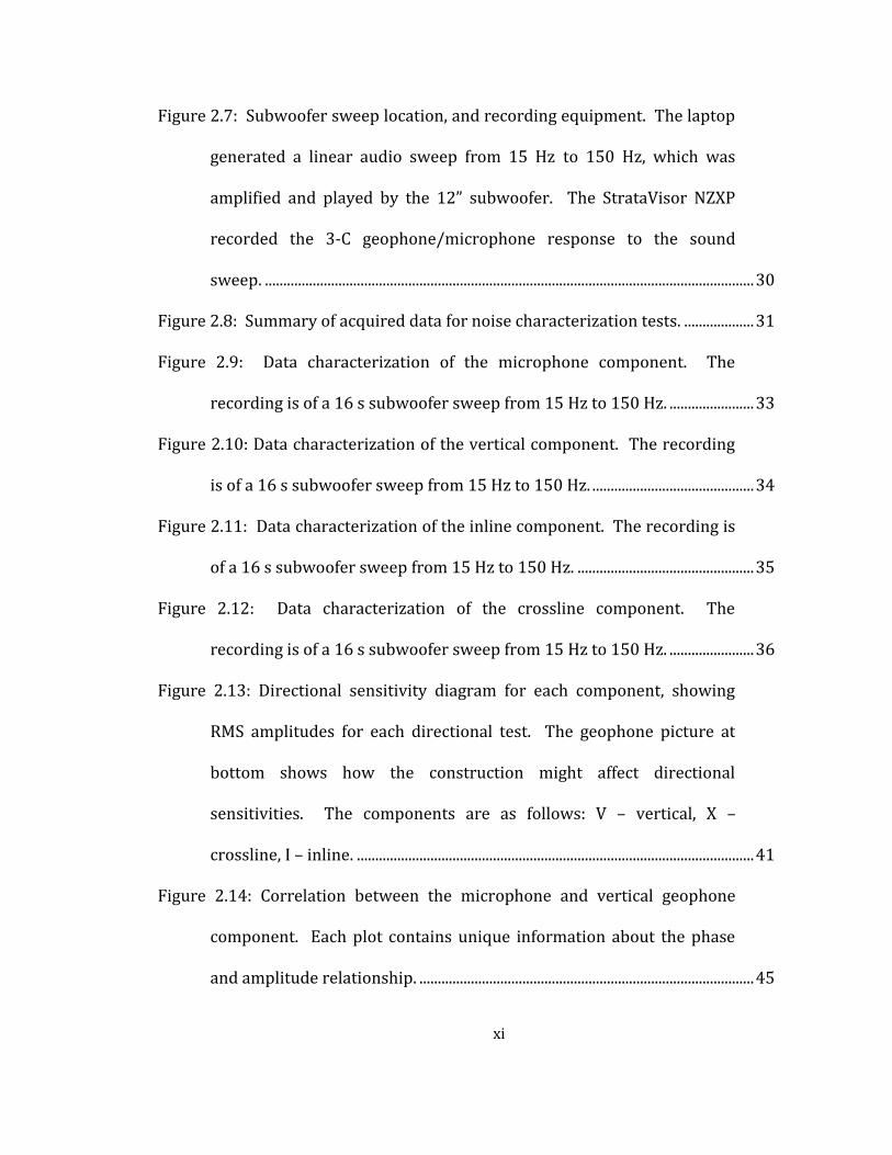
Figure 2.7: Subwoofer sweep location, and recording equipment. The laptop

generated a linear audio sweep from 15 Hz to 150 Hz, which was

amplified and played by the 12” subwoofer. The StrataVisor NZXP

recorded the 3-C geophone/microphone response to the sound

sweep. ..................................................................................................................................... 30

Figure 2.8: Summary of acquired data for noise characterization tests. ................... 31

Figure 2.9: Data characterization of the microphone component. The

recording is of a 16 s subwoofer sweep from 15 Hz to 150 Hz. ....................... 33

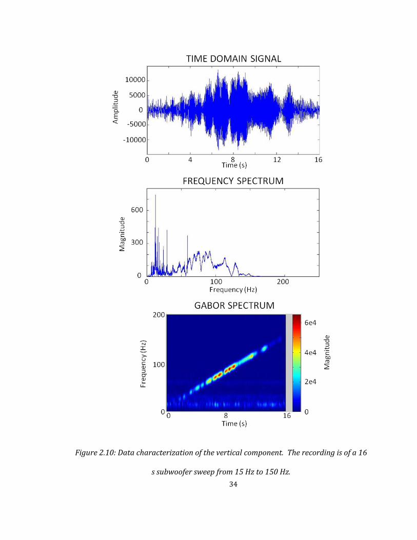
Figure 2.10: Data characterization of the vertical component. The recording

is of a 16 s subwoofer sweep from 15 Hz to 150 Hz. ............................................ 34

Figure 2.11: Data characterization of the inline component. The recording is

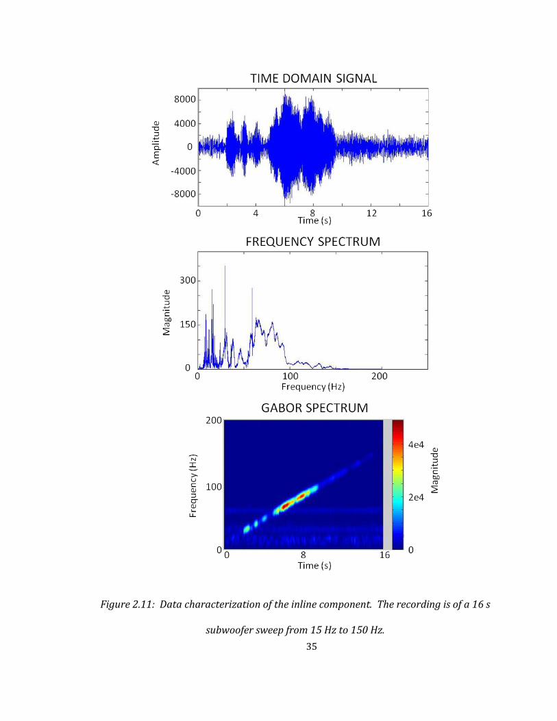
of a 16 s subwoofer sweep from 15 Hz to 150 Hz. ................................................ 35

Figure 2.12: Data characterization of the crossline component. The

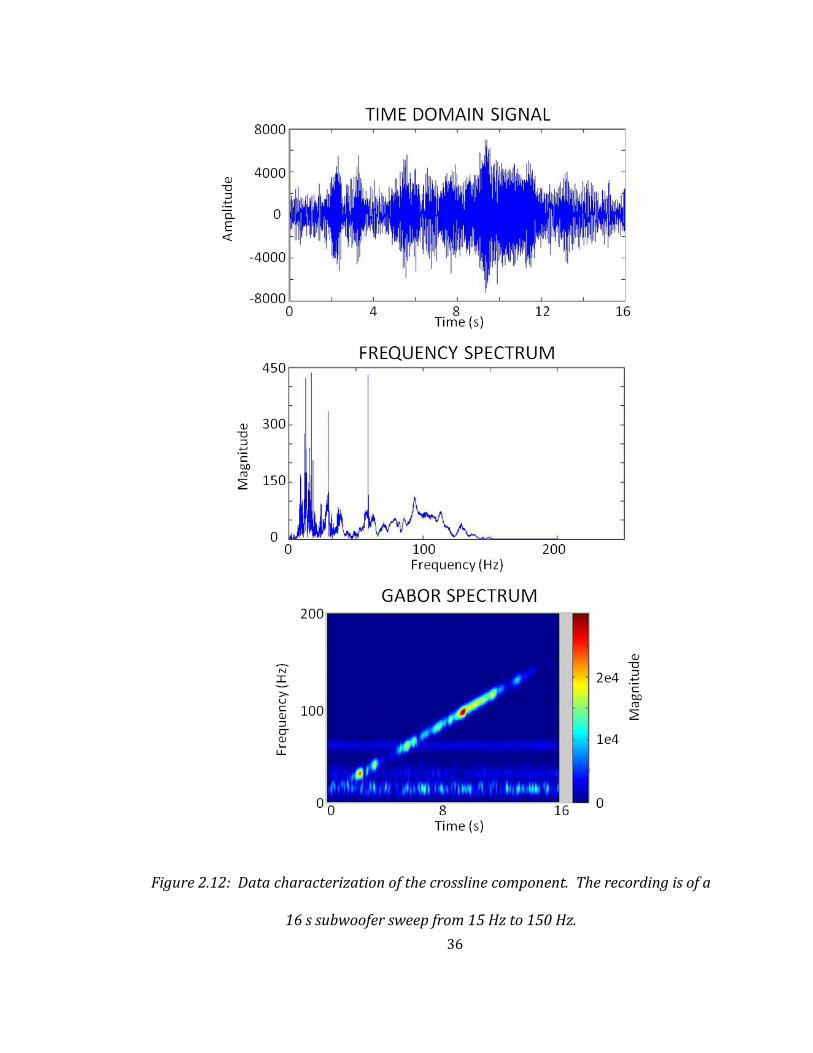
recording is of a 16 s subwoofer sweep from 15 Hz to 150 Hz. ....................... 36

Figure 2.13: Directional sensitivity diagram for each component, showing

RMS amplitudes for each directional test. The geophone picture at

bottom shows how the construction might affect directional

sensitivities. The components are as follows: V – vertical, X –

crossline, I – inline. ............................................................................................................ 41

Figure 2.14: Correlation between the microphone and vertical geophone

component. Each plot contains unique information about the phase

and amplitude relationship. ........................................................................................... 45

xii

Figure 2.15: Cartoon process showing frequency-band correlation.

Frequency slices are taken from the Gabor domain (a) and (b), then

cross-correlated. The result is placed in the appropriate frequency

slot in (c). ............................................................................................................................... 46

Figure 2.16: Correlation between the microphone and inline geophone

component. ........................................................................................................................... 48

Figure 2.17: Correlation between the microphone and crossline geophone

component. ........................................................................................................................... 49

Figure 2.18: Maximum cross-correlation value of each geophone record and

the microphone record. Values further from the center indicate

higher correlations, and higher similarities. ............................................................ 51

Figure 2.19: Maximum correlation lag offset for each geophone component,

after cross-correlation with the microphone. Values further from the

first ring indicate positive lag offsets, and values lower than the first

ring indicate negative lag offsets. A bigger lag offset indicates larger

phase mismatch between that component and microphone. ........................... 52

Figure 2.20: Gabor spectra multiplication of each geophone component with

the microphone. The results show where both geophone and

microphone responses are strong. The vertical component has the

largest response. The inline response is stronger than the crossline

response due to the incoming direction of the sound sweep. ........................... 54

xiii

Figure 3.1: The "pillow-top" vibration isolation system. The piezo

microphone is placed inside a felt pocket, surrounded by polyester

fibers. These springy fibers dampen vibrations that affect the

microphone. Shown attached atop a 3-C geophone. ............................................ 57

Figure 3.2: Survey location and schematic. Satellite imagery of the northern

portion of the UH Coastal Center, near La Marque, Texas. The blue

circle shows the approximate 4-C prototype geophone position,

defined as 0 m. The red line indicates the shot line, from -2.5 m to

702.5 m shot at a 5 m interval. Imagery source (Google Maps, 2012) .......... 58

Figure 3.3: Vertical component correlated shot gather. Displayed using 500

ms AGC, showing the first 2.5 s of the record. Note the very weak air-

wave. ........................................................................................................................................ 61

Figure 3.4: Crossline component correlated shot gather. Displayed using

500 ms AGC, showing the first 2.5 s of the record. ................................................ 62

Figure 3.5: Inline component correlated shot gather. Displayed using 500

ms AGC, showing the first 2.5 s of the record. Note the strong air-

wave. There is also shear-wave refractions located beneath the air-

wave. ........................................................................................................................................ 63

Figure 3.6: Geophone amplitude decay comparison for the air-wave arrival.

The vertical component amplitude decays much faster than the

horizontal components. ................................................................................................... 66

xiv

Figure 3.7: Microphone component correlated shot gather. Displayed using

500 ms AGC, showing the first 2.5 s of the record. Note the head-wave

and reflections present in the record. ........................................................................ 68

Figure 3.8: Microphone recorded air-wave amplitude decay. The

microphone decay rate is similar to the horizontal geophone

components. ......................................................................................................................... 69

Figure 3.9: A simplified diagram of the microphone case. The diagram shows

a cross-section running through the middle of the microphone and

case. .......................................................................................................................................... 76

Figure 3.10: The finished microphone case. The steel plates on top allow the

microphone to be stomped on, while the blue nylon keeps the

microphone dry. .................................................................................................................. 77

Figure 3.11: The finished prototype 4-C geophone, sitting atop a 3-C

geophone in the field. ........................................................................................................ 77

Figure 4.1: Amplitude kernels for each geophone component. The crossline

and inline kernels are almost identical. This is the result of averaging

kernels from multiple directions, removing directional dependency

from kernel response. ....................................................................................................... 82

Figure 4.2: Filter process diagram. Data inputs are amplitude modulated for

distance, then transformed to the frequency-domain. Three

amplitude kernels are applied to the microphone spectrum to

estimate the magnitude of noise for each geophone component. These

xv

noise-magnitude estimates are combined with the corresponding

geophone phase to create noise-spectra estimates. Each noise

spectrum is converted back to the time-domain, where the newly

created noise signal is subtracted from the geophone signal. The post-

acquisition filter includes an additional step; it applies a windowing

function to the noise signal to isolate the air-noise for improved

precision during air-noise removal. ............................................................................ 86

Figure 4.3: Vertical component: comparison of the real-time and windowed

post-processing filters, to the original vertical seismogram and the

filter-produced noise estimate. ..................................................................................... 90

Figure 4.4: Vertical component: comparison of the high-cut and FK-domain

velocity filters, to the original vertical seismogram and the windowed

post-processing filter. ....................................................................................................... 91

Figure 4.5: Crossline component: comparison of the real-time and windowed

post-processing filters, to the original crossline seismogram and the


Figure 4.6: Crossline component: comparison of the high-cut and FK-domain

velocity filters, to the original crossline seismogram and the

windowed post-processing filter. ................................................................................ 94

Figure 4.7: Inline component: comparison of the real-time and windowed

post-processing filters, to the original inline seismogram and the


xvi

Figure 4.8: Inline component: comparison of the high-cut and FK-domain

velocity filters, to the original inline seismogram and the windowed

post-processing filter. ....................................................................................................... 97

Figure 5.1: Microphone raw shot gather compared to the vertical raw shot

gather, both with 500 ms AGC. The presence of reflectors and head-

wave are seen in the microphone record. .............................................................. 101

Figure 5.2: Inline component windowed post-processing filter results, both

with 500 ms AGC. The filter removes most of the air-wave, without

affecting any seismic arrivals...................................................................................... 104

Figure B-1: Receiver-based noise cancellation system. Horizontal geophones

(22) are used to record and cancel surface waves (20) from the

vertical geophones (18). Microphones (24) are used to cancel wind

noise. A strong motion geophone (28) is located near a mechanical

noise source (26) to record and cancel ground noise on nearby

geophones. (Crews and Martinez, 1989) .............................................................. 114

Figure B-2: Source-based noise cancellation system. A speaker (16) located

at a seismic source (12) plays a tone or series of tones during a

seismic shot. This tone is received by a microphone (28) and is used

to cancel source based air-noise from recorded geophone signal (26).

(Sallas and Moerig, 2002) ............................................................................................ 115

1

CHAPTER 1: INTRODUCTION

Noise in seismic records can obscure desirable signals, cause a loss of detail,

and even create spurious events; thus degrading the seismic image. Fortunately,

some noises are removed relatively easily by stacking data or using filters (FK,

frequency, etc.). However, not all noise is so easily removed. Air-noise is a

significant source of noise in seismograms. The most obvious source of air-noise is

from the seismic shot. Whether it is dynamite or vibroseis, all seismic sources

generate air-pressure waves that travel past the geophones. As this noise travels

across the geophone spread, it vibrates the geophones, creating noise in the seismic

records. There are other ways for air-noise to affect a geophone. Since the near

surface is porous, pressure waves from sound can more easily penetrate into the

subsurface. This creates additional vibrations, which can be recorded by the

geophone.

To remove air-noise from seismic records, its character and strength in the

geophone signal must be estimated. A microphone can be used for this purpose. It

will record the air-wave, and other air-noise that affects the geophone. There will

not necessarily be a direct correlation between the microphone and geophone

recorded air-noise. The purpose of this thesis was to characterize the relationship

between microphone-recorded air-noise and geophone-recorded air-noise. The

knowledge obtained in this process was used to create a real-time filter, which can

2

be applied in the field to remove air-noise from the geophone signal before it is

recorded by the seismograph.

A series of experiments were undertaken to understand the microphone-

geophone relationship. Controlled experiments were performed to determine the

geophone’s response to sound coming from different angles, as well as for sounds of

varying frequencies. By recording these sounds using the microphone at the same

time, a microphone-geophone transfer function was calculated, which was used in

the development of the filter. An experiment was also performed to determine how

the geophone-microphone pair reacts to sounds coming from different distances.

This experiment was performed in the field because large source-receiver offsets

are required to fully characterize the relationship.

After the relationship between microphone and geophone was well

characterized, a filter was designed to work in real-time. The filter was tested on

field data, in real-time and post-acquisition settings, to determine its effectiveness.

This filter could be programmed to a digital signal processor, and built into a special

4-C geophone, to create a geophone that automatically removes air-noise before

outputting clean signal. However, this implementation was not tested here, and is

reserved for future work. Before analyzing the microphone-geophone relationship,

an overview of the many ways air-noise can affect the geophone is presented.

3

1.1: Types of noise that affect a geophone

The operational portion of any geophone contains two main parts, a

reference frame and oscillating proof mass. Analog geophones contain a coil that

surrounds a moveable magnet (or a metal case surrounding moveable coils), while

MEMS accelerometers contain two electrodes that sandwich a moveable mass acting

as a capacitor. The reference frame being stationary is only relative. In reality, the

reference frame moves about the mass, while the “moving” mass stays still. For

geophones, it is this relative movement of the mass compared to the reference

frame that creates the desired signal. In the analog geophone, the velocity of the

moving magnet creates a voltage in the surrounding coil. In the MEMS

accelerometer, accelerations displace the mass (capacitor) changing the voltage

detected in the reference frame (Hons and Stewart, 2007). The reference frame

(referred to as the geophone element) attaches to a housing structure (the

geophone case) that contains a spike for planting in the ground. Visual diagrams for

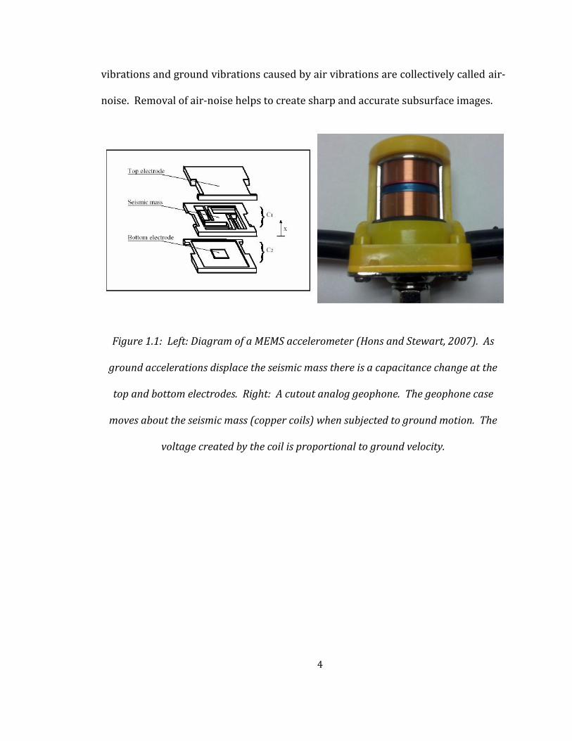
analog and MEMS geophones can be seen in Figure 1.1.

In a seismic experiment, vibrations from seismic waves will move the spike

and thus the entire geophone (except for the proof mass). These movements are

recorded and analyzed later to create seismic images. Other, undesirable, vibrations

can affect the geophone in two ways; spurious ground vibrations cause movement

in the geophone through the spike embedded in the ground, or air vibrations

directly move the geophone case without transferring through the spike first. All of

these excess movements of the geophone create noise in the seismic record. Air

4

vibrations and ground vibrations caused by air vibrations are collectively called air-

noise. Removal of air-noise helps to create sharp and accurate subsurface images.

Figure 1.1: Left: Diagram of a MEMS accelerometer (Hons and Stewart, 2007). As

ground accelerations displace the seismic mass there is a capacitance change at the

top and bottom electrodes. Right: A cutout analog geophone. The geophone case

moves about the seismic mass (copper coils) when subjected to ground motion. The

voltage created by the coil is proportional to ground velocity.

5

1.1.1: Noise that affects the geophone case

The most common source of air-noise for any seismic survey is the air-blast

or air-wave. This acoustic wave is produced, and defined, by the source used in the

seismic experiment; air-wave is created by a seismic vibrator and air-blast by an

impulsive source. These waves travel through the air at the speed of sound (346

m/s at 25° C) and strike the geophone case, causing it to shake. This creates noise in

the seismic record.

Wind is another common phenomenon that creates noise in seismic records.

This disturbance, which directly affects the geophone case, is created by turbulent

eddies and vortices, referred to as turbules. These turbules, carried by the wind,

vibrate the geophone case as they move past (Hedlin and Raspet, 2003). This type

of wind noise is generally spatially coherent and can be followed across geophone

traces. The correlation coefficient, for wind-induced noise, between seismic traces

is estimated by

,

where x and y are the downwind and crosswind geophone spacing, respectively

(Shields, 2005). is the spatial wavenumber of the turbulent wind flow and is

given by

6

where is the wind velocity and is the frequency of the pressure fluctuations

produced, i.e. the frequency of the noise present on the geophone. The remaining

coefficients are given by

(

)

Identification and reduction of wind noise is very important for infrasonic

monitoring stations. These stations are used to detect sub-audible signal (<20 Hz),

which can be used to identify nuclear blasts, battlefield noise, meteors entering the

earth’s atmosphere, even large storms and tornados. Infrasonic monitoring stations

use either microbarometers or specially designed microphones capable of detecting

sound down to, and below, 1 Hz (Kromer, 2000; Shields, 2005). These infrasonic

microphones would be suitable for air-noise cancellation from seismic records.

The final sources of air-induced noise are transient sources. These sources of

noise are finite in time and may or may not affect multiple geophones at a time.

Examples of transient noises include vehicles, helicopter and other aircraft, oilfield

equipment, and human/animal movement near geophones. Essentially, transient

sources are any noise source not previously categorized.

7

1.1.2: Noise that affects the geophone elements

Air-noise does not solely affect geophones by directly striking their case. Air-

noise may couple to the ground and directly vibrate the geophone elements to

produce unwanted noise. This can happen in three separate ways. One of the more

obvious is wind-noise coupling. Wind not only directly vibrates the geophone case

but every structure that impedes its movement: trees, buildings, even grass become

secondary sources of noise (Stewart, 1998). Wind may also directly couple to the

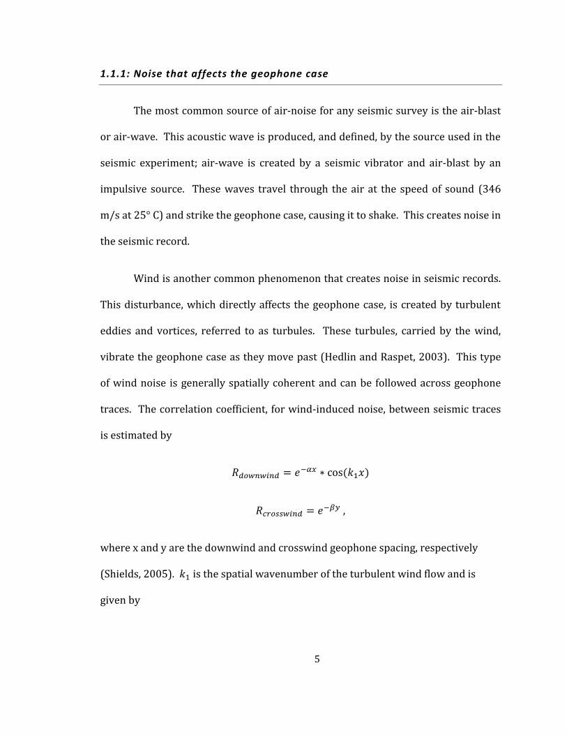
ground without shaking any intermediary structure. Withers et al. (1996)

performed wind noise experiments in a remote area in New Mexico, which had

gentle topography and little surface vegetation. Even with the favorable conditions,

there was still significant ground-coupled wind noise. A covered seismometer near

the surface (30 cm burial) detected wind noise at speeds as low as 3 m/s (10.8

km/hr). Furthermore, a magnitude 1.6 event was barely detectable at a wind speed

of 8 m/s (28.8 km/hr), as seen in Figure 1.2.

It has been recommended to bury geophones to decrease wind effects. Bland

and Gallant (2001) measured a 3 dB increase in signal-to-noise ratio for every 10 cm

of burial depth. The total depth to bury the geophone depends on desired noise

reduction, but Withers et al. (1996) generally recommend a minimum burial depth

of 43 m.

8

Figure 1.2: Left: Power spectral density (PSD) comparison of wind noise (lower line)

and M1.6 seismic event (upper line) at varying wind speeds for a geophone located on

the surface and at depth. Right: Superimposed M1.6 event on time records of wind

noise at varying wind speeds for a geophone located at the surface and at depth.

(Withers et al., 1996)

Since the acoustic impedance of air is not zero, there will be some transfer of

energy from any compressional wave in the air, to the ground. However, the

coupling of acoustic-to-seismic waves is 1000 times larger than would be calculated

from direct transmission (Sabatier et al., 1986a). This increase in energy transfer

occurs because the air-to-ground interface is not sharp. The upper few decimeters

(or in some cases meters) of the earth are highly porous and permeable. Any sound

that propagates in air will easily penetrate into this region. A Biot-Stall medium is a

good model for this near-surface layer. A Biot-Stall medium is poroelestic, with fully

interconnected pores saturated by fluid. Both the matrix and pore fluid are

considered isotropic, homogeneous, and elastic. In the near-surface case, the matrix

9

is the unconsolidated sediments, and the pore fluid is air. A peculiar feature of a

Biot-Stall medium is its ability to support the propagation of two compressional

waves, one fast and one slow. The fast compressional wave is analogous to a P-wave

and travels mainly through the matrix. The slow compressional wave, on the other

hand, travels mostly through the pore fluid. This slow wave is rarely detected in

seismic records because it is extremely attenuative. In the air-noise case, acoustic

waves propagating in the air refract more easily to the slow wave than the fast wave

in the poroelestic, near-surface layer. Energy is then transferred from the air-filled

pores to the matrix creating seismic motion (Sabatier et al., 1986b). Because the

slow wave in the ground is highly attenuative, the ground motion will only occur

directly beneath the current location of the acoustic wave in the air (Sabatier et al.,

1986a). In other words, an air-wave will not spawn a leading or lagging

compressional seismic wave.

Lastly, air-waves may also couple to the ground through Rayleigh waves.

This occurs when the air-wave velocity is similar to the phase velocity of the

Rayleigh wave. Since surface waves are dispersive, only one frequency of the

Rayleigh-wave’s fundamental mode will have a phase velocity matching the air-

wave. Thus, the ground roll created by the air-wave will oscillate at a singular

frequency. Furthermore, the group velocity is typically one half that of the air-wave

velocity (Press and Ewing, 1951). This means that the induced ground roll will lag

behind the air-wave that created it. For any given point in the subsurface, the wave

train that follows the air-wave arrival will last for the same duration as the original

10

travel time of the air-wave. An example for clarification, for an air-wave velocity of

345 m/s, the Rayleigh-wave with a matching phase velocity will have a group

velocity of approximately 173 m/s. The air-wave will constantly couple to this

Rayleigh-wave. However, due to the Rayleigh-wave’s lower group velocity, all

induced ground roll will lag behind. After one second, the air-wave will have

travelled 345 m, but the first-coupled Rayleigh-wave will have only travelled 173 m.

If a geophone were place at this point, it would detect the air-wave arrival at one

second, which would be immediately followed by the monofrequency Rayleigh-

wave. Due to the lagging velocity, the Rayleigh-wave train continues for one second

after the air-wave arrival. An example cartoon of the expected geophone response

to air-noise and seismic signal is shown in Figure 1.3. This air-to-ground roll

coupling will occur for any air-wave, adding noise to seismic recordings.

Ground roll coupling is not a one-way transfer from air-to-ground, Rayleigh

waves can also produce motion in the air. Ground-to-air coupling is the inverse of

the air-to-ground process. The ground roll at the correct phase velocity will couple

to the air and create a train of constant frequency air-waves that trail behind (Press

and Ewing, 1951). Air-waves created by ground roll are an additional source of

noise that affects the geophone case, and may be detectable by microphone. While

the air-noise effects of ground roll can be actively cancelled, the concept cannot be

extended to the cancellation of all ground roll from geophone records. This is due to

the differing frequency content of the microphone-recorded ground-to-air-wave

signal and the seismic ground roll recorded by the geophone. For every seismic

11

event (hammer shot, Vibroseis) there is a concurrent air event. Any receiving

geophone will record signal from both events. To extract the seismic data, the air-

noise signature must be determined and removed from the geophone record.

Figure 1.3: Synthetic seismic traces showing a vertical geophone's response to a

theoretical impulse source, according to Press and Ewing (1951). The top trace shows

the source generated ground motion only. The bottom trace shows the air-wave

induced ground motion. The true geophone response will be the combination of these

two traces. Time is to scale, however the amplitude response is not.

12

1.2: Prior work

The CREWES project, at the University of Calgary, has worked extensively in

the area of geophone noise cancellation using microphones. The work performed

here is the continuation and advancement of that performed by CREWES. The first

experiment performed was during a hospital implosion in Calgary, Alberta in 1998.

It was found that the microphone and geophone recordings of the blast showed

distinct similarities. In fact, the air-blast recorded by the microphone appeared to

be 180° out of phase with the blast recorded by the geophone. Thus, the sum of the

microphone and geophone traces showed a reasonable reduction of air-blast.

Stewart (1998) proposed two noise-reducing multi-sensors that could be used

during seismic data acquisition to reduce the noise present in geophone records.

One of the sensors was a multi-channel setup consisting of microphone data

recorded simultaneously with geophone data. The microphone data could later be

used to filter noise as necessary. The other sensor consisted of an integrated

filtering circuit that would use the signal from a collocated microphone to suppress

noise in the geophone signal. Noise cancellation was performed at geophone level

and the resulting signal was output to the data acquisition system as an unfiltered

geophone would. A comparison of these sensor types can be seen in Figure 1.4.

13

Figure 1.4: Schematic of noise cancelling geophones. Left: A multi-channel system,

which would record geophone and microphone data separately to be processed after

acquisition. Right: A single channel system, which would record and filter air-noise at

the geophone. The data acquisition system would record “clean” data.

(Stewart, 1998)

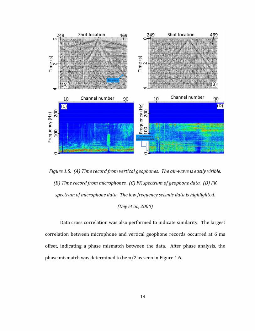
Dey et al. (2000) used a multiline survey to analyze the capability of air-blast

attenuation using microphones. A 3.8 km seismic survey was performed with

microphones and vertical geophones placed every 20 m, 3-C geophones every 10 m,

and vibroseis shot points every 20m. The data from each sensor type were

compared for similarities in time and FK domains, which are shown in Figure 1.5.

The microphone record contained not only the air-blast but also significant low

frequency data, although it was spatially aliased.

14

Figure 1.5: (A) Time record from vertical geophones. The air-wave is easily visible.

(B) Time record from microphones. (C) FK spectrum of geophone data. (D) FK

spectrum of microphone data. The low frequency seismic data is highlighted.

(Dey et al., 2000)

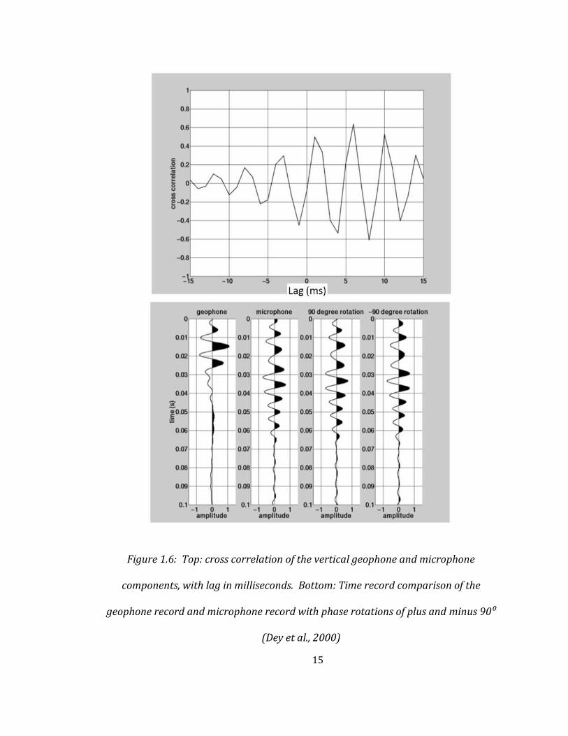
Data cross correlation was also performed to indicate similarity. The largest

correlation between microphone and vertical geophone records occurred at 6 ms

offset, indicating a phase mismatch between the data. After phase analysis, the

phase mismatch was determined to be π/2 as seen in Figure 1.6.

15

Figure 1.6: Top: cross correlation of the vertical geophone and microphone

components, with lag in milliseconds. Bottom: Time record comparison of the

geophone record and microphone record with phase rotations of plus and minus 90⁰

(Dey et al., 2000)

16

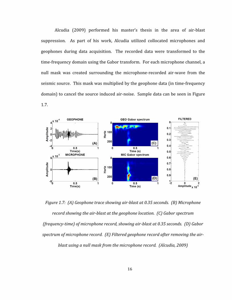
Alcudia (2009) performed his master’s thesis in the area of air-blast

suppression. As part of his work, Alcudia utilized collocated microphones and

geophones during data acquisition. The recorded data were transformed to the

time-frequency domain using the Gabor transform. For each microphone channel, a

null mask was created surrounding the microphone-recorded air-wave from the

seismic source. This mask was multiplied by the geophone data (in time-frequency

domain) to cancel the source induced air-noise. Sample data can be seen in Figure

1.7.

Figure 1.7: (A) Geophone trace showing air-blast at 0.35 seconds. (B) Microphone

record showing the air-blast at the geophone location. (C) Gabor spectrum

(frequency-time) of microphone record, showing air-blast at 0.35 seconds. (D) Gabor

spectrum of microphone record. (E) Filtered geophone record after removing the air-

blast using a null mask from the microphone record. (Alcudia, 2009)

17

CHAPTER 2: NOISE CHARACTERIZATION STUDY

The basis of any noise-cancellation filter is the estimation and removal of

noise present in an incoming signal. There are various classes of noise cancellation

filters, including static and active. Static filters are ones that do not change over

time; however, this does not mean they are simple. Active filters, on the other hand,

change over time using input from any number of sources. Each class of filter has

particular strengths and weaknesses. Static filters are typically smaller than active

filters, in terms of resources used. They are also less flexible, requiring an accurate

characterization of the noise present in the signal. Active filters are much more

flexible since their parameters change over time. This means that the noise does not

need to be perfectly characterized, as any discrepancies are updated in real-time.

The goal of the noise characterization test is to determine how sound affects a 3C

geophone, which will help determine which filtering method is best suited for

removing air-noise.

2.1: Hardware design

A significant portion of the work presented here revolves around the design

and use of a prototype 4-C geophone. The prototype consists of a 3-C geophone

with an attached microphone. The overall design of the prototype has evolved

through multiple iterations throughout the course of this thesis.

18

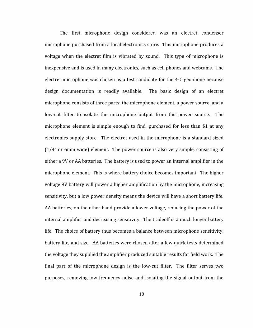
The first microphone design considered was an electret condenser

microphone purchased from a local electronics store. This microphone produces a

voltage when the electret film is vibrated by sound. This type of microphone is

inexpensive and is used in many electronics, such as cell phones and webcams. The

electret microphone was chosen as a test candidate for the 4-C geophone because

design documentation is readily available. The basic design of an electret

microphone consists of three parts: the microphone element, a power source, and a

low-cut filter to isolate the microphone output from the power source. The

microphone element is simple enough to find, purchased for less than $1 at any

electronics supply store. The electret used in the microphone is a standard sized

(1/4” or 6mm wide) element. The power source is also very simple, consisting of

either a 9V or AA batteries. The battery is used to power an internal amplifier in the

microphone element. This is where battery choice becomes important. The higher

voltage 9V battery will power a higher amplification by the microphone, increasing

sensitivity, but a low power density means the device will have a short battery life.

AA batteries, on the other hand provide a lower voltage, reducing the power of the

internal amplifier and decreasing sensitivity. The tradeoff is a much longer battery

life. The choice of battery thus becomes a balance between microphone sensitivity,

battery life, and size. AA batteries were chosen after a few quick tests determined

the voltage they supplied the amplifier produced suitable results for field work. The

final part of the microphone design is the low-cut filter. The filter serves two

purposes, removing low frequency noise and isolating the signal output from the

19

battery. Typical low-cut filters could be 60 Hz or higher, depending on use. The

desired microphone for the 4-C geophone cannot use a standard design; it requires

lower frequency content to pass through to the recording system. A corner

frequency of about 1 Hz was chosen to keep the signal output isolated while still

allowing sound in the seismic band to pass.

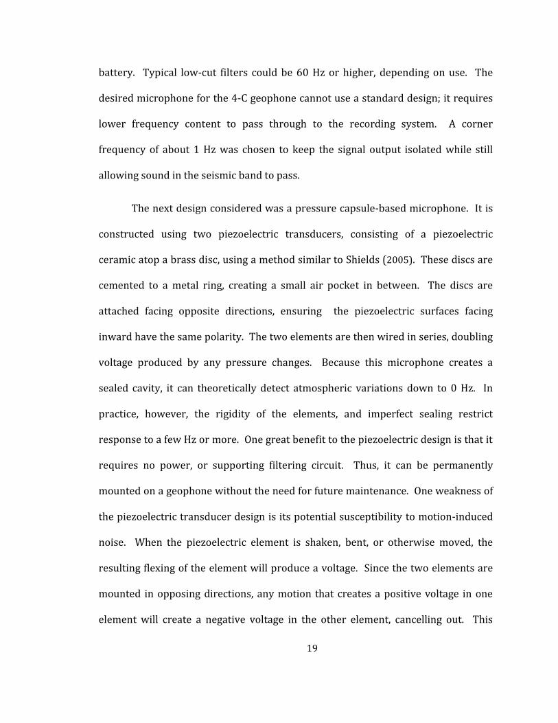
The next design considered was a pressure capsule-based microphone. It is

constructed using two piezoelectric transducers, consisting of a piezoelectric

ceramic atop a brass disc, using a method similar to Shields (2005). These discs are

cemented to a metal ring, creating a small air pocket in between. The discs are

attached facing opposite directions, ensuring the piezoelectric surfaces facing

inward have the same polarity. The two elements are then wired in series, doubling

voltage produced by any pressure changes. Because this microphone creates a

sealed cavity, it can theoretically detect atmospheric variations down to 0 Hz. In

practice, however, the rigidity of the elements, and imperfect sealing restrict

response to a few Hz or more. One great benefit to the piezoelectric design is that it

requires no power, or supporting filtering circuit. Thus, it can be permanently

mounted on a geophone without the need for future maintenance. One weakness of

the piezoelectric transducer design is its potential susceptibility to motion-induced

noise. When the piezoelectric element is shaken, bent, or otherwise moved, the

resulting flexing of the element will produce a voltage. Since the two elements are

mounted in opposing directions, any motion that creates a positive voltage in one

element will create a negative voltage in the other element, cancelling out. This

20

process is not perfect, so small left-over charges can remain to be detected by the

recording system. To prevent motion-induced noise, the piezoelectric pressure

capsule can be mounted in a vibration-damping housing.

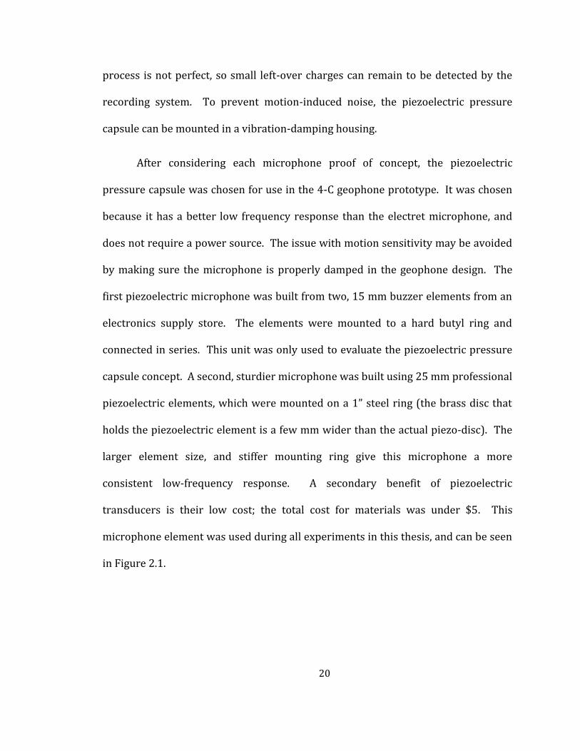
After considering each microphone proof of concept, the piezoelectric

pressure capsule was chosen for use in the 4-C geophone prototype. It was chosen

because it has a better low frequency response than the electret microphone, and

does not require a power source. The issue with motion sensitivity may be avoided

by making sure the microphone is properly damped in the geophone design. The

first piezoelectric microphone was built from two, 15 mm buzzer elements from an

electronics supply store. The elements were mounted to a hard butyl ring and

connected in series. This unit was only used to evaluate the piezoelectric pressure

capsule concept. A second, sturdier microphone was built using 25 mm professional

piezoelectric elements, which were mounted on a 1” steel ring (the brass disc that

holds the piezoelectric element is a few mm wider than the actual piezo-disc). The

larger element size, and stiffer mounting ring give this microphone a more

consistent low-frequency response. A secondary benefit of piezoelectric

transducers is their low cost; the total cost for materials was under $5. This

microphone element was used during all experiments in this thesis, and can be seen

in Figure 2.1.

21

Figure 2.1: Final piezoelectric microphone. A brass disc contains a piezoelectric

ceramic on one side. This is glued, facing inward, to a steel ring. A similar element is

glued on the opposite side of the ring. The two pairs of wires coming from the

microphone are from each piezo-element. They are wired in series to double the

voltage produced by pressure changes on the microphone.

2.2: Experimental setup

The noise characterization tests consist of playing a sound and recording the

geophone’s response, while in a controlled environment. A microphone is

collocated with the geophone during the test to create a microphone-to-geophone

transfer function. This function describes how a sound recorded by a microphone

relates to the same sound recorded by a geophone. To conduct the test, all

unnecessary sources of noise, both mechanical and air vibrations, need to be

reduced or accounted for. This ensures the transfer function created by the

22

characterization tests only applies to sounds picked up by both microphone and

geophone, and nothing else.

The chosen test site was a large room, in Science and Research Building 1 on

the University of Houston campus, which has thick cinder-block walls. To ensure

lower levels of background noise the characterization tests were run at night. The

only significant source of noise was an industrial air conditioning system, located

outside the test room approximately 20 m away. This system created noise from 10

Hz to 30 Hz, mostly within narrow bands at 15 Hz and 30 Hz. To isolate the test

setup a vibration isolation platform was built (see Figure 2.2). The isolation system

consists of a series of springs connected to a wooden frame, suspended from the

ceiling. The springs slightly stretch and compress when subjected to vibration,

damping motion for the suspended platform. Air-noise created by the air

conditioner still affects the test setup, but this is an unexpected benefit, as it allows

for the analysis of low-frequency sound.

There is also a small amount of 60 Hz noise from electrical interference. To

reduce this noise, all lights were turned off during testing and ancillary electronic

devices were unplugged from their outlets. Any record stored by the StrataVisor

seismic recording system can be converted from amplitude to true voltage using a

scaling factor, determined by the system recording gain. For the noise

characterization tests, this scaling factor is 1.6985e-4 mV. To determine the

23

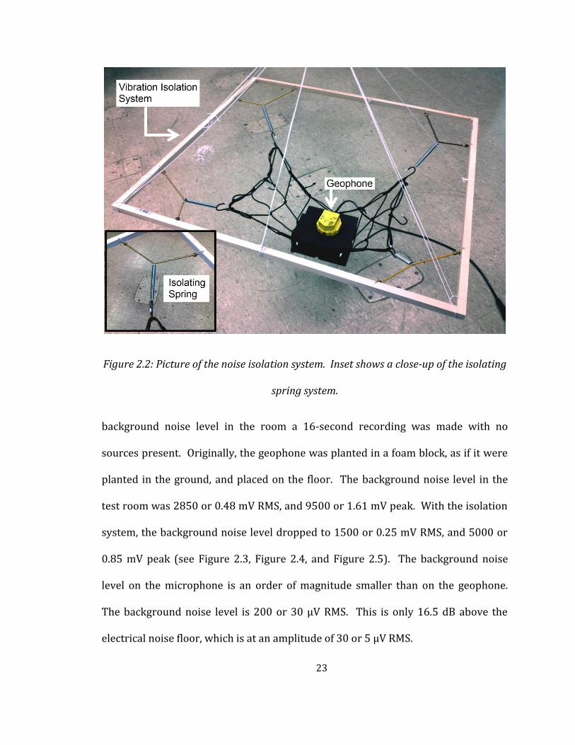
Figure 2.2: Picture of the noise isolation system. Inset shows a close-up of the isolating

spring system.

background noise level in the room a 16-second recording was made with no

sources present. Originally, the geophone was planted in a foam block, as if it were

planted in the ground, and placed on the floor. The background noise level in the

test room was 2850 or 0.48 mV RMS, and 9500 or 1.61 mV peak. With the isolation

system, the background noise level dropped to 1500 or 0.25 mV RMS, and 5000 or

0.85 mV peak (see Figure 2.3, Figure 2.4, and Figure 2.5). The background noise

level on the microphone is an order of magnitude smaller than on the geophone.

The background noise level is 200 or 30 μV RMS. This is only 16.5 dB above the

electrical noise floor, which is at an amplitude of 30 or 5 μV RMS.

24

Figure 2.3: Time domain signal comparison of the isolation system used to decouple

the test apparatus from background noise vibrations. The isolation system decreases

background noise levels to less than half, compared to no isolation system.

25

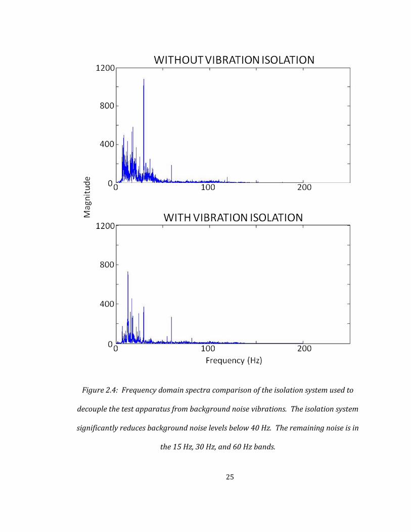
Figure 2.4: Frequency domain spectra comparison of the isolation system used to

decouple the test apparatus from background noise vibrations. The isolation system

significantly reduces background noise levels below 40 Hz. The remaining noise is in

the 15 Hz, 30 Hz, and 60 Hz bands.

26

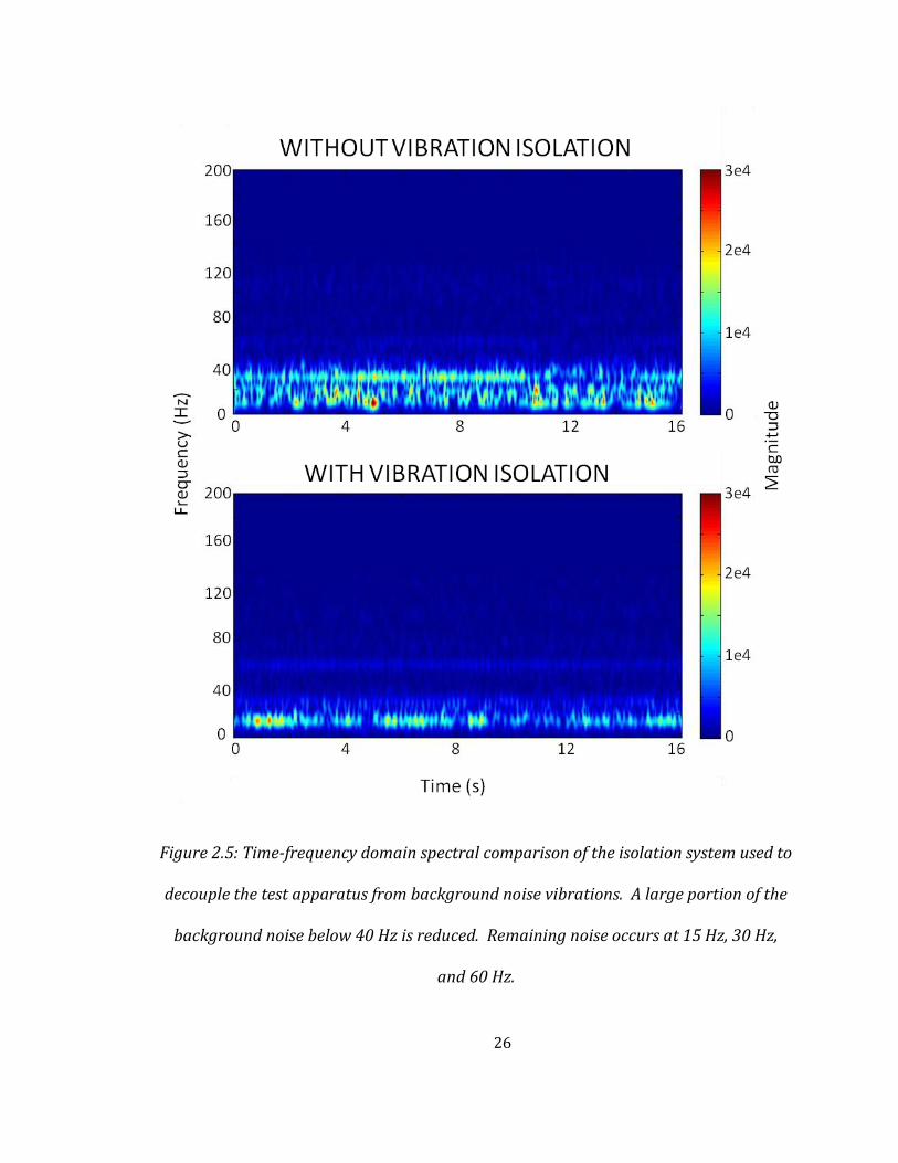
Figure 2.5: Time-frequency domain spectral comparison of the isolation system used to

decouple the test apparatus from background noise vibrations. A large portion of the

background noise below 40 Hz is reduced. Remaining noise occurs at 15 Hz, 30 Hz,

and 60 Hz.

27

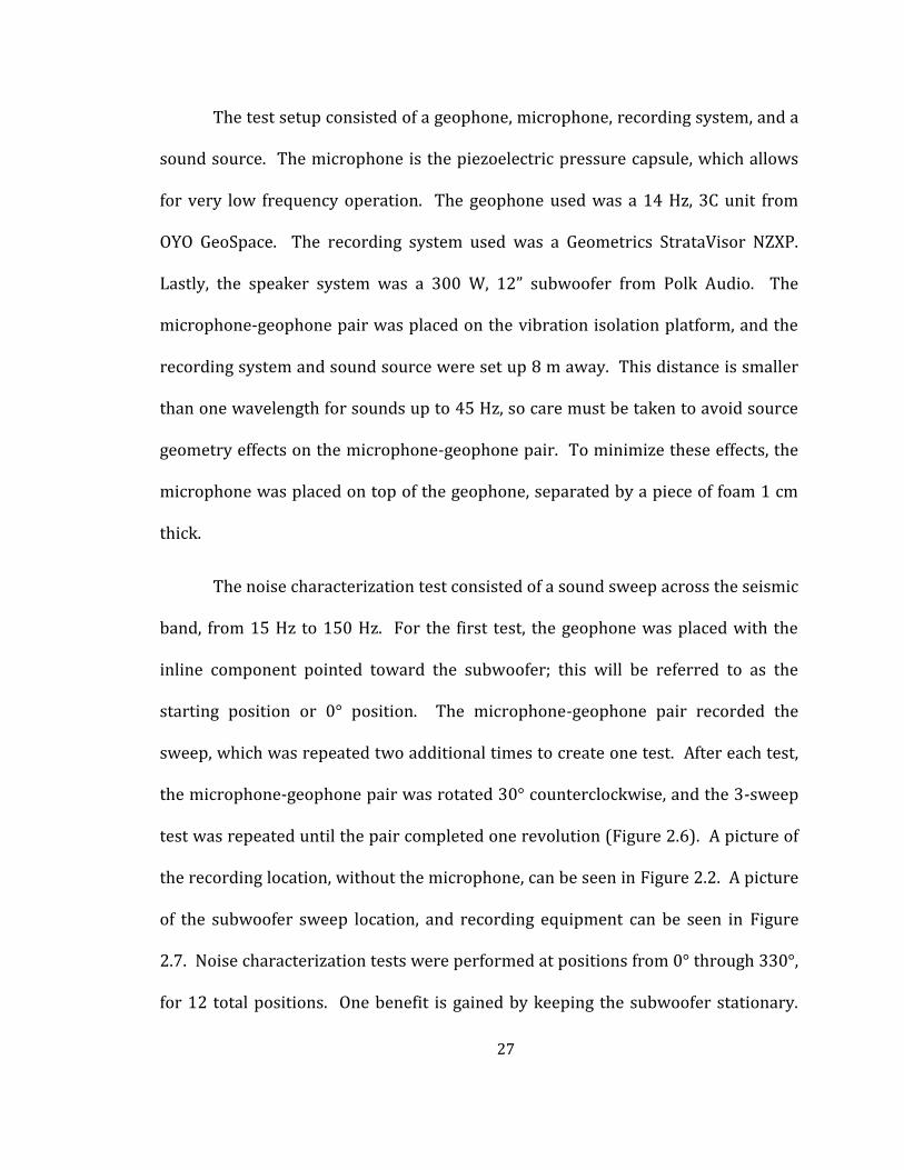
The test setup consisted of a geophone, microphone, recording system, and a

sound source. The microphone is the piezoelectric pressure capsule, which allows

for very low frequency operation. The geophone used was a 14 Hz, 3C unit from

OYO GeoSpace. The recording system used was a Geometrics StrataVisor NZXP.

Lastly, the speaker system was a 300 W, 12” subwoofer from Polk Audio. The

microphone-geophone pair was placed on the vibration isolation platform, and the

recording system and sound source were set up 8 m away. This distance is smaller

than one wavelength for sounds up to 45 Hz, so care must be taken to avoid source

geometry effects on the microphone-geophone pair. To minimize these effects, the

microphone was placed on top of the geophone, separated by a piece of foam 1 cm

thick.

The noise characterization test consisted of a sound sweep across the seismic

band, from 15 Hz to 150 Hz. For the first test, the geophone was placed with the

inline component pointed toward the subwoofer; this will be referred to as the

starting position or 0° position. The microphone-geophone pair recorded the

sweep, which was repeated two additional times to create one test. After each test,

the microphone-geophone pair was rotated 30° counterclockwise, and the 3-sweep

test was repeated until the pair completed one revolution (Figure 2.6). A picture of

the recording location, without the microphone, can be seen in Figure 2.2. A picture

of the subwoofer sweep location, and recording equipment can be seen in Figure

2.7. Noise characterization tests were performed at positions from 0° through 330°,

for 12 total positions. One benefit is gained by keeping the subwoofer stationary.

28

Sound propagates from the subwoofer in all directions. These sounds may bounce

off walls constructively or destructively interfering with the main wave. By keeping

the subwoofer in one position, these interferences remain constant, and can be

identified in the seismogram as frequencies with a consistently weak, or strong,

response.

There are a few positions of note: at 90° the crossline component points at

the source, at 180° the inline component points away from the source, and at 270°

the crossline component points away from the source. The positions at 0°, 90°, 180°

and 270° had additional 3-sweep tests performed, in which the microphone was

aligned with the other two geophone components, inline and crossline. These tests

were used to confirm the omnidirectional response of the microphone. After all

noise characterization tests were acquired, a final test was conducted at the 0°

position to determine test repeatability. A table describing each test position is seen

in Figure 2.8.

29

Figure 2.6: Apparent shot points, relative to the microphone/geophone setup.

Subwoofer sweeps were performed three times at each position, which were 30° apart.

Due to space constraints, it was actually the microphone/geophone pair that rotated,

while the subwoofer remained in one position. The subwoofer was located eight

meters from the test apparatus.

30

Figure 2.7: Subwoofer sweep location, and recording equipment. The laptop

generated a linear audio sweep from 15 Hz to 150 Hz, which was amplified and played

by the 12” subwoofer. The StrataVisor NZXP recorded the 3-C geophone/microphone

response to the sound sweep.

31

Position name

Geophone orientation

Microphone orientation

Number of tests at position

Type of test

1V 0° Vertical 2 Background noise 1V 0° Vertical 3 Sound sweep 1X 0° Crossline 3 Sound sweep 1I 0° Inline 3 Sound sweep 2V 30° Vertical 3 Sound sweep 3V 60° Vertical 3 Sound sweep 4V 90° Vertical 3 Sound sweep 4X 90° Crossline 3 Sound sweep 4I 90° Inline 3 Sound sweep 5V 120° Vertical 3 Sound sweep 6V 150° Vertical 3 Sound sweep 7V 180° Vertical 3 Sound sweep 7X 180° Crossline 3 Sound sweep 7I 180° Inline 3 Sound sweep 8V 210° Vertical 3 Sound sweep 9V 240° Vertical 3 Sound sweep 10V 270° Vertical 3 Sound sweep 10X 270° Crossline 3 Sound sweep 10I 270° Inline 3 Sound sweep 11V 300° Vertical 3 Sound sweep 12V 330° Vertical 3 Sound sweep 1V 0° Vertical 3 Sound sweep

Figure 2.8: Summary of acquired data for noise characterization tests.

2.3: Data analysis

The noise characterization study produced 65 data files from 22 tests. Given

the amount of data, a standardized method was conceived to summarize and

analyze the results. Before fully analyzing the noise characterization tests the data

should be looked over, to become familiar with the sound sweep and expected

response. Summaries of data from the first noise characterization test (geophone at

0°) are shown below for each component: microphone, vertical, inline, and crossline

32

(Figure 2.9, Figure 2.10, Figure 2.11, and Figure 2.12 respectively). The subplots

within help characterize the sound recorded by each component. The time domain

signal shows exactly what was recorded. The FFT chart displays the overall

frequency content of the signal. The FFT cannot distinguish short sounds, of high

amplitude from long sounds, of low amplitude. This means that the sound sweep

cannot be distinguished from background noise from the nearby air conditioners.

The only way to distinguish between these sounds is by converting to the time-

frequency domain using the Gabor transform. The Gabor transform is a type of

STFT that applies a Gaussian window. This type of window strikes a good balance

between time localization and frequency localization, which is usually a trade off

when converting to the time-frequency domain. The window length used for this

analysis was 10 ms. In essence, this gives a windowed Fourier transform every 10

ms across the entire signal, showing exactly which signals are present at each point

in time.

33

Figure 2.9: Data characterization of the microphone component. The recording is of a

16 s subwoofer sweep from 15 Hz to 150 Hz.

34

Figure 2.10: Data characterization of the vertical component. The recording is of a 16

s subwoofer sweep from 15 Hz to 150 Hz.

35

Figure 2.11: Data characterization of the inline component. The recording is of a 16 s

subwoofer sweep from 15 Hz to 150 Hz.

36

Figure 2.12: Data characterization of the crossline component. The recording is of a

16 s subwoofer sweep from 15 Hz to 150 Hz.

37

The noise characterization test was of a sound sweep from 15 Hz to 150 Hz

over 15 s, with a total recording time of 16 s. This simulates an uncorrelated

seismic trace from a field survey using a vibroseis source. The upper limit of the

sweep is seen by the microphone FFT, but the range from 130 Hz to 150 Hz is much

weaker. Because the subwoofer has an integrated high-cut filter of 120 Hz, any

sound above this frequency is played at a reduced volume. The lower frequency

limit is also unclear due to the subwoofer’s resonant frequency, which is 23 Hz.

Again, if any sound is below this frequency it will be played at a significantly

reduced volume. While the true sound sweep was from 15 Hz to 150 Hz, the

operational response is closer to 25 Hz to 130 Hz. From the time-domain signal of

the microphone, the mid frequencies appear to be stronger (70 Hz to 100 Hz),

compared to frequencies on the edges of the range (similarly indicated by the FFT).

This means that the subwoofers output is not flat across the frequency range of the

sound sweep. While the signal response of the subwoofer is important to keep in

mind, it should not affect the characterization of sound between geophone and

microphone. The important thing is that the microphone-geophone pair records the

same sound, whatever it may be. Looking at the Gabor transform of a signal is a

quick way to determine the presence of background noise. The Gabor transform for

the microphone clearly shows the sweep, and shows very little background noise in

the seismic band. This is confirmed by the time domain signal, which shows

background noise levels of 500. The RMS amplitude for this trace is 2250 and the

peak amplitude is 8400. This gives a RMS signal-to-noise ratio of 4.5:1, and a peak

38

signal-to-noise ratio of 16.8:1. Having a low background noise level on the

microphone is important, because any noise present may be combined into the

geophone record during noise cancellation.

The vertical geophone component has a similar story, compared to the

microphone. From the FFT, the high frequency data weakens past 130 Hz and cuts

off at 150 Hz, but the low frequency data are different. Below 30 Hz, the sound

sweep entangles with background noise from nearby air conditioning units. This

noise is low in amplitude, but constant throughout the entire test, creating a large

response on the FFT. There is also 60 Hz power line noise, which manifests as a

spike on the FFT. The Gabor transform shows the sweep down to near 20 Hz or 25

Hz. The spectrum does help separate the sweep from the air conditioning and

power line noise. Since these noise sources are constant, they show up as lines of

constant frequency in the Gabor transform. The air conditioning noise is contained

below 30 Hz, with two distinct sources of noise at 15 Hz and 30 Hz. The power line

noise is seen at 60 Hz. The RMS background noise is around 1000 with peak

amplitudes of 2000, and the RMS of the signal is 3750 with peak amplitude near

14000. This gives a RMS signal-to-noise ratio of 3.75:1 and peak signal-to-noise

ratio of 7:1.

The inline geophone component is quite different from the vertical

component. The FFT of the inline component mostly recorded signal from 50 Hz to

100 Hz, with small additions at lower frequencies. The background seems stronger

on this component, due to the sweep signal being weaker. There is general

39

background hum below 25 Hz; large noise spikes at 15 Hz and 30 Hz, from the air

conditioner; and 60 Hz power-line noise. The Gabor transform confirms the signal

bandwidth from the FFT, although it is able to separate the 30 Hz signal from the 30

Hz background noise. The background noise is clearer on the Gabor transform,

compared to the vertical component. The background noise level remains the same

as the vertical component, RMS amplitude of 1000 and peak amplitude of 2000.

However, the signal is weaker, with a RMS amplitude of 2350 and a peak amplitude

of 9500. This gives a RMS signal-to-noise ratio of 2.4:1 and peak signal-to-noise

ratio of 4.8:1.

The crossline component is even weaker than the inline component because

it is orthogonal to the sound source. The FFT shows a weak response across the

entire frequency band. The background noise from the air conditioner and power

line appear even stronger, dictating the scale of the FFT diagram. Even with the

relatively stronger response of the noise, the Gabor transform is still able to

distinguish the sweep. Again, the background noise has a RMS amplitude of 1000

and a peak amplitude of 2000, with a RMS signal level of 1700 and a peak amplitude

of 8000. This gives a RMS signal-to-noise ratio of 1.7:1 and peak signal-to-noise

ratio of 4:1.

Now that a general description of each component has been determined, full

analysis of the geophone’s response to noise coming from different angles can be

performed. To determine the strength of each geophone component’s response to

sound, RMS and peak amplitude values are calculated. When plotted as a function of

40

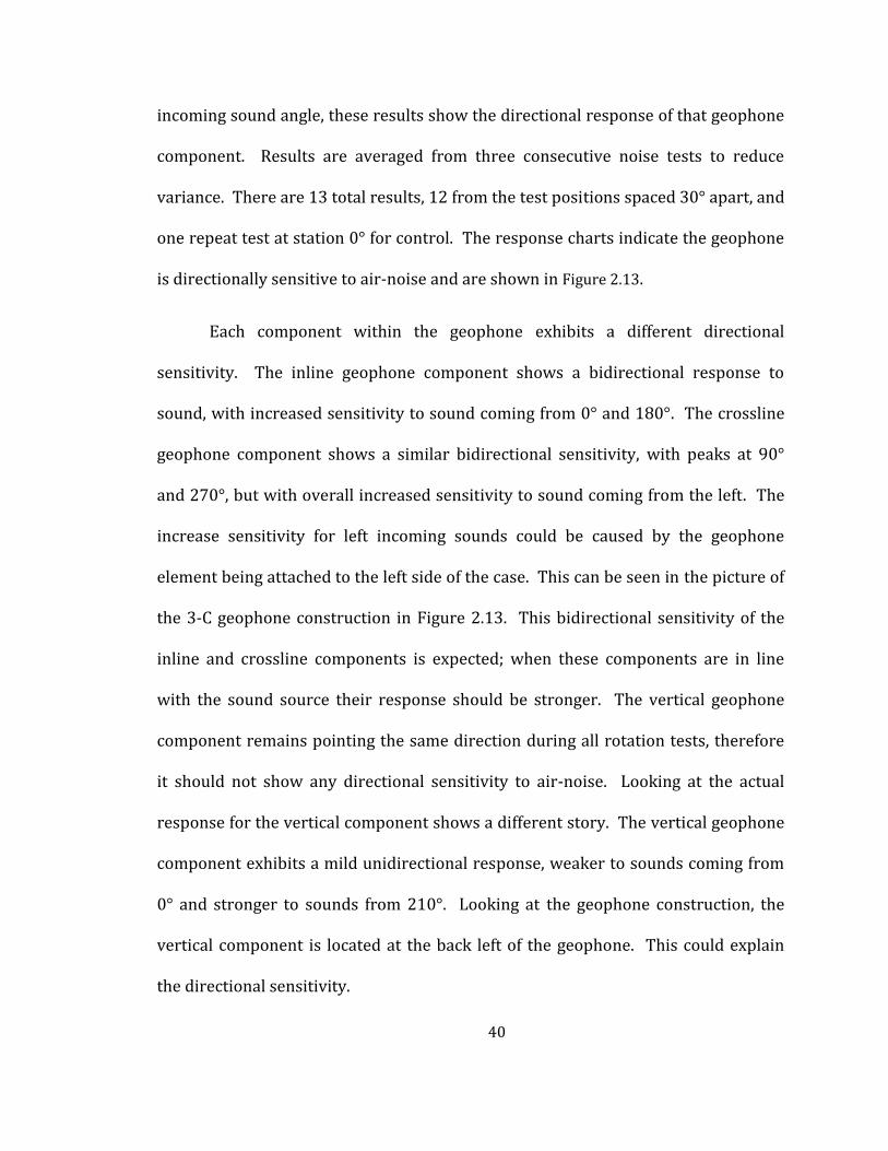
incoming sound angle, these results show the directional response of that geophone

component. Results are averaged from three consecutive noise tests to reduce

variance. There are 13 total results, 12 from the test positions spaced 30° apart, and

one repeat test at station 0° for control. The response charts indicate the geophone

is directionally sensitive to air-noise and are shown in Figure 2.13.

Each component within the geophone exhibits a different directional

sensitivity. The inline geophone component shows a bidirectional response to

sound, with increased sensitivity to sound coming from 0° and 180°. The crossline

geophone component shows a similar bidirectional sensitivity, with peaks at 90°

and 270°, but with overall increased sensitivity to sound coming from the left. The

increase sensitivity for left incoming sounds could be caused by the geophone

element being attached to the left side of the case. This can be seen in the picture of

the 3-C geophone construction in Figure 2.13. This bidirectional sensitivity of the

inline and crossline components is expected; when these components are in line

with the sound source their response should be stronger. The vertical geophone

component remains pointing the same direction during all rotation tests, therefore

it should not show any directional sensitivity to air-noise. Looking at the actual

response for the vertical component shows a different story. The vertical geophone

component exhibits a mild unidirectional response, weaker to sounds coming from

0° and stronger to sounds from 210°. Looking at the geophone construction, the

vertical component is located at the back left of the geophone. This could explain

the directional sensitivity.

41

Figure 2.13: Directional sensitivity diagram for each component, showing RMS

amplitudes for each directional test. The geophone picture at bottom shows how the

construction might affect directional sensitivities. The components are as follows: V –

vertical, X – crossline, I – inline.

42

The microphone used in these experiments was built to be omnidirectional.

To confirm this, the microphone was tested at the same time, and in the same way,

as the geophone. The directional response diagram is also in Figure 2.13. The

diagram shows the microphone to be very nearly omnidirectional, producing an

equal response to sounds from all directions.

2.4: Microphone-to-geophone transfer function

To determine the microphone-to-geophone transfer function we must find

how they relate in two ways, amplitude and phase. The amplitude comparison

sounds simple enough; it is the difference in amplitude between the microphone

and geophone records, but stopping here would be a gross approximation. In the

characterization study, the geophone and microphone responded differently to

sounds of different frequencies. Typically, the microphone has a stronger response

to high frequency sounds while the geophone has a stronger response to lower

frequency sounds. Thus, the amplitude relation must be determined at each

frequency of interest. Phase shows similar frequency dependent response, so its

transfer function will need to be determined for each frequency. Each geophone

component has a different response to sound, so each component will have its own

unique transfer function. A useful, first-order comparison between two signals is

the cross-correlation. This operation calculates the similarity between two signals

at various offsets. The higher the correlation value, the more similar the two signals

43

are to each other. If the correlation value is one, the two signals contain the same

signal, but might still have differing amplitudes.

Figure 2.14 shows the comparison between the microphone and vertical

geophone component for the first noise characterization test at 0° (position 1V).

The cross-correlation shows a strong positive correlation, 0.58, but this value does

not occur at the expected 0 ms offset. It instead occurs at -5 ms, indicating an

overall phase mismatch between the microphone and geophone signals. Looking at

the phase chart confirms this, the microphone record remains close to 180° out of

phase with the geophone record, for the entire band of the sound sweep. One issue

with using a simple correlation to determine signal similarity is that it does not

consider these phase differences. A more effective correlation method would occur

in the frequency domain, where phase differences arise as offsets in a cross-

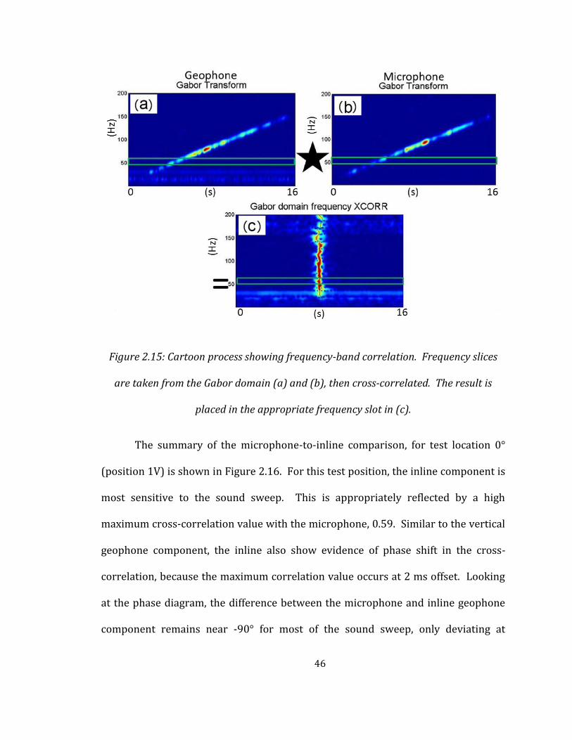
correlation. I call this type of correlation “frequency-band correlation,” and it is

done in the Gabor domain. The process is as follows. After performing the Gabor

transform of the microphone and geophone data, the resulting spectra are divided

into frequency slices. These are, essentially, spectrally decomposed signals. These

spectrally decomposed signals can then cross-correlated in much the same manner

as normal signal cross-correlation. Each frequency band from the microphone

spectrum is cross-correlated with the corresponding frequency band from the

geophone spectrum. After every frequency band correlation is calculated, they are

all stacked atop each other to produce a frequency dependent similarity chart

between the two signals. A cartoon of the process is shown in Figure 2.15, with the

44

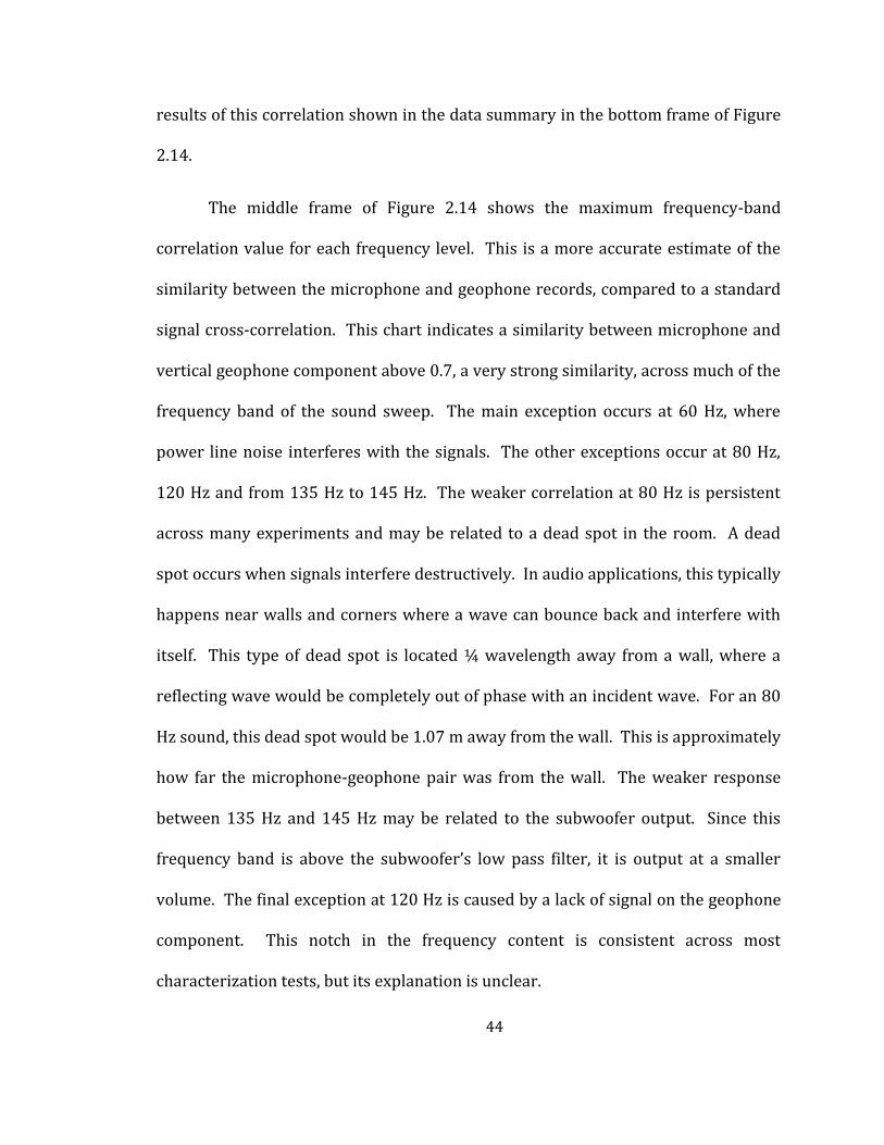
results of this correlation shown in the data summary in the bottom frame of Figure

2.14.

The middle frame of Figure 2.14 shows the maximum frequency-band

correlation value for each frequency level. This is a more accurate estimate of the

similarity between the microphone and geophone records, compared to a standard

signal cross-correlation. This chart indicates a similarity between microphone and

vertical geophone component above 0.7, a very strong similarity, across much of the

frequency band of the sound sweep. The main exception occurs at 60 Hz, where

power line noise interferes with the signals. The other exceptions occur at 80 Hz,

120 Hz and from 135 Hz to 145 Hz. The weaker correlation at 80 Hz is persistent

across many experiments and may be related to a dead spot in the room. A dead

spot occurs when signals interfere destructively. In audio applications, this typically

happens near walls and corners where a wave can bounce back and interfere with

itself. This type of dead spot is located ¼ wavelength away from a wall, where a

reflecting wave would be completely out of phase with an incident wave. For an 80

Hz sound, this dead spot would be 1.07 m away from the wall. This is approximately

how far the microphone-geophone pair was from the wall. The weaker response

between 135 Hz and 145 Hz may be related to the subwoofer output. Since this

frequency band is above the subwoofer’s low pass filter, it is output at a smaller

volume. The final exception at 120 Hz is caused by a lack of signal on the geophone

component. This notch in the frequency content is consistent across most

characterization tests, but its explanation is unclear.

45

Figure 2.14: Correlation between the microphone and vertical geophone component.

Each plot contains unique information about the phase and amplitude relationship.

46

Figure 2.15: Cartoon process showing frequency-band correlation. Frequency slices

are taken from the Gabor domain (a) and (b), then cross-correlated. The result is

placed in the appropriate frequency slot in (c).

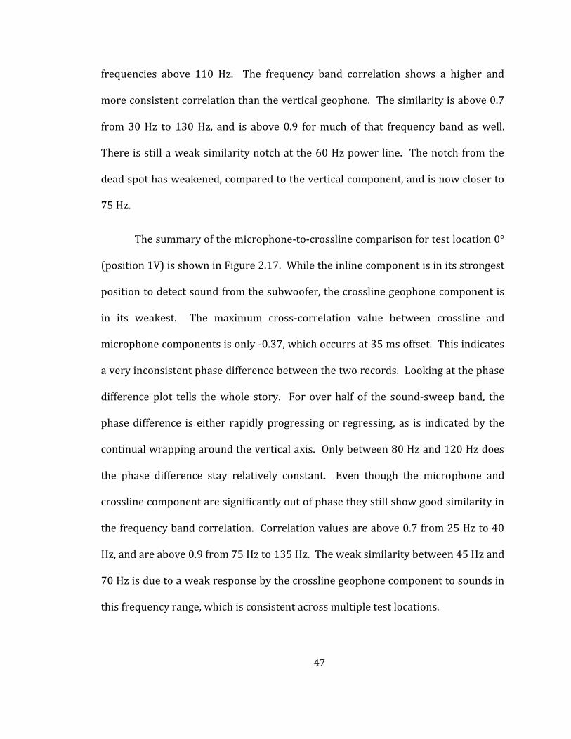
The summary of the microphone-to-inline comparison, for test location 0°

(position 1V) is shown in Figure 2.16. For this test position, the inline component is

most sensitive to the sound sweep. This is appropriately reflected by a high

maximum cross-correlation value with the microphone, 0.59. Similar to the vertical

geophone component, the inline also show evidence of phase shift in the cross-

correlation, because the maximum correlation value occurs at 2 ms offset. Looking

at the phase diagram, the difference between the microphone and inline geophone

component remains near -90° for most of the sound sweep, only deviating at

47

frequencies above 110 Hz. The frequency band correlation shows a higher and

more consistent correlation than the vertical geophone. The similarity is above 0.7

from 30 Hz to 130 Hz, and is above 0.9 for much of that frequency band as well.

There is still a weak similarity notch at the 60 Hz power line. The notch from the

dead spot has weakened, compared to the vertical component, and is now closer to

75 Hz.

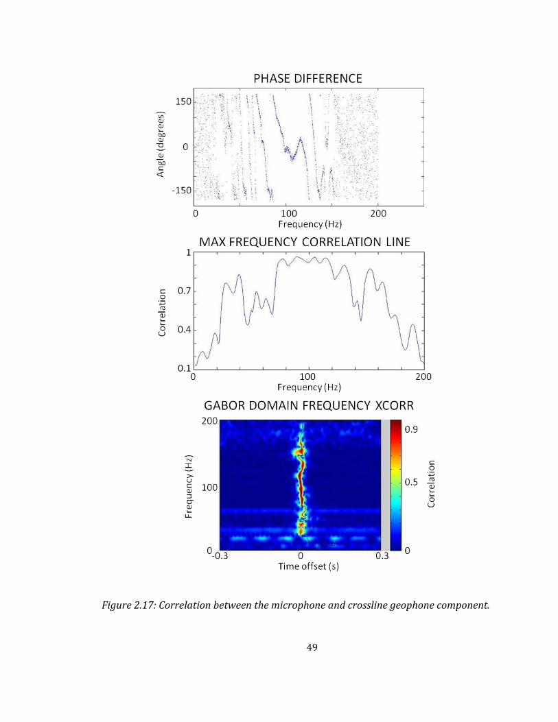
The summary of the microphone-to-crossline comparison for test location 0°

(position 1V) is shown in Figure 2.17. While the inline component is in its strongest

position to detect sound from the subwoofer, the crossline geophone component is

in its weakest. The maximum cross-correlation value between crossline and

microphone components is only -0.37, which occurrs at 35 ms offset. This indicates

a very inconsistent phase difference between the two records. Looking at the phase

difference plot tells the whole story. For over half of the sound-sweep band, the

phase difference is either rapidly progressing or regressing, as is indicated by the

continual wrapping around the vertical axis. Only between 80 Hz and 120 Hz does

the phase difference stay relatively constant. Even though the microphone and

crossline component are significantly out of phase they still show good similarity in

the frequency band correlation. Correlation values are above 0.7 from 25 Hz to 40

Hz, and are above 0.9 from 75 Hz to 135 Hz. The weak similarity between 45 Hz and

70 Hz is due to a weak response by the crossline geophone component to sounds in

this frequency range, which is consistent across multiple test locations.

48

Figure 2.16: Correlation between the microphone and inline geophone component.

49

Figure 2.17: Correlation between the microphone and crossline geophone component.

50

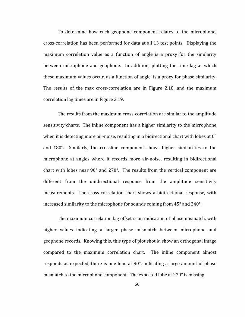
To determine how each geophone component relates to the microphone,

cross-correlation has been performed for data at all 13 test points. Displaying the

maximum correlation value as a function of angle is a proxy for the similarity

between microphone and geophone. In addition, plotting the time lag at which

these maximum values occur, as a function of angle, is a proxy for phase similarity.

The results of the max cross-correlation are in Figure 2.18, and the maximum

correlation lag times are in Figure 2.19.

The results from the maximum cross-correlation are similar to the amplitude

sensitivity charts. The inline component has a higher similarity to the microphone

when it is detecting more air-noise, resulting in a bidirectional chart with lobes at 0°

and 180°. Similarly, the crossline component shows higher similarities to the

microphone at angles where it records more air-noise, resulting in bidirectional

chart with lobes near 90° and 270°. The results from the vertical component are

different from the unidirectional response from the amplitude sensitivity

measurements. The cross-correlation chart shows a bidirectional response, with

increased similarity to the microphone for sounds coming from 45° and 240°.

The maximum correlation lag offset is an indication of phase mismatch, with

higher values indicating a larger phase mismatch between microphone and

geophone records. Knowing this, this type of plot should show an orthogonal image

compared to the maximum correlation chart. The inline component almost

responds as expected, there is one lobe at 90°, indicating a large amount of phase

mismatch to the microphone component. The expected lobe at 270° is missing

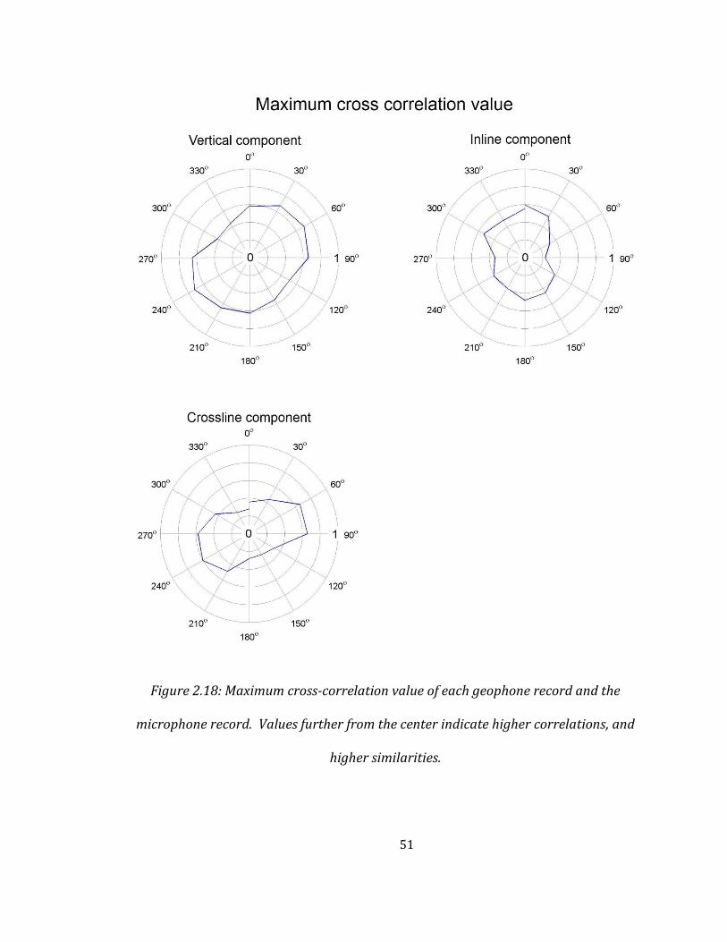
51

Figure 2.18: Maximum cross-correlation value of each geophone record and the

microphone record. Values further from the center indicate higher correlations, and

higher similarities.

52

Figure 2.19: Maximum correlation lag offset for each geophone component, after

cross-correlation with the microphone. Values further from the first ring indicate

positive lag offsets, and values lower than the first ring indicate negative lag offsets. A

bigger lag offset indicates larger phase mismatch between that component and

microphone.

53

however. The crossline component responds as expected, with lobes at 0° and 180°,

indicating high phase mismatch to sounds coming from those angles. The vertical

component continues to show results contrasting with its earlier unidirectional

sensitivity. There are lobes at 120° and 330°, indicating increased phase mismatch

to sounds coming from those directions.

The final piece of information to come from the microphone-geophone

transfer function is the amplitude relationship. The frequency-band correlation is

an indication of similarity between two signals in the time-frequency domain, but it

does not give any information about amplitude. A quick way to compare amplitudes

in the time-frequency domain is to multiply two Gabor spectra together. This has

been performed for the first test at 0°, position 1V (Figure 2.20). Stronger values

indicate frequencies where both the geophone and microphone are strong, but not

necessarily how strong the geophone is compared to the microphone. All charts

show relatively strong responses between 70 Hz and 100 Hz, with the inline

component being the strongest. This could be caused by an increase in

geophone/microphone response to the sound sweep, or by an increase in

subwoofer output. What is important is the comparison between geophone

channels. The inline component shows a stronger response than the crossline

component. For this test position, the inline component is pointing toward the

subwoofer, thus it should have a stronger response.

54

Figure 2.20: Gabor spectra multiplication of each geophone component with the

microphone. The results show where both geophone and microphone responses are

strong. The vertical component has the largest response. The inline response is

stronger than the crossline response due to the incoming direction of the sound sweep.

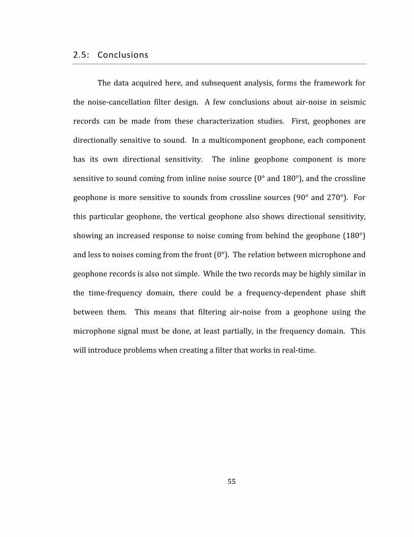
55

2.5: Conclusions

The data acquired here, and subsequent analysis, forms the framework for

the noise-cancellation filter design. A few conclusions about air-noise in seismic

records can be made from these characterization studies. First, geophones are

directionally sensitive to sound. In a multicomponent geophone, each component

has its own directional sensitivity. The inline geophone component is more

sensitive to sound coming from inline noise source (0° and 180°), and the crossline

geophone is more sensitive to sounds from crossline sources (90° and 270°). For

this particular geophone, the vertical geophone also shows directional sensitivity,

showing an increased response to noise coming from behind the geophone (180°)

and less to noises coming from the front (0°). The relation between microphone and

geophone records is also not simple. While the two records may be highly similar in

the time-frequency domain, there could be a frequency-dependent phase shift

between them. This means that filtering air-noise from a geophone using the

microphone signal must be done, at least partially, in the frequency domain. This

will introduce problems when creating a filter that works in real-time.

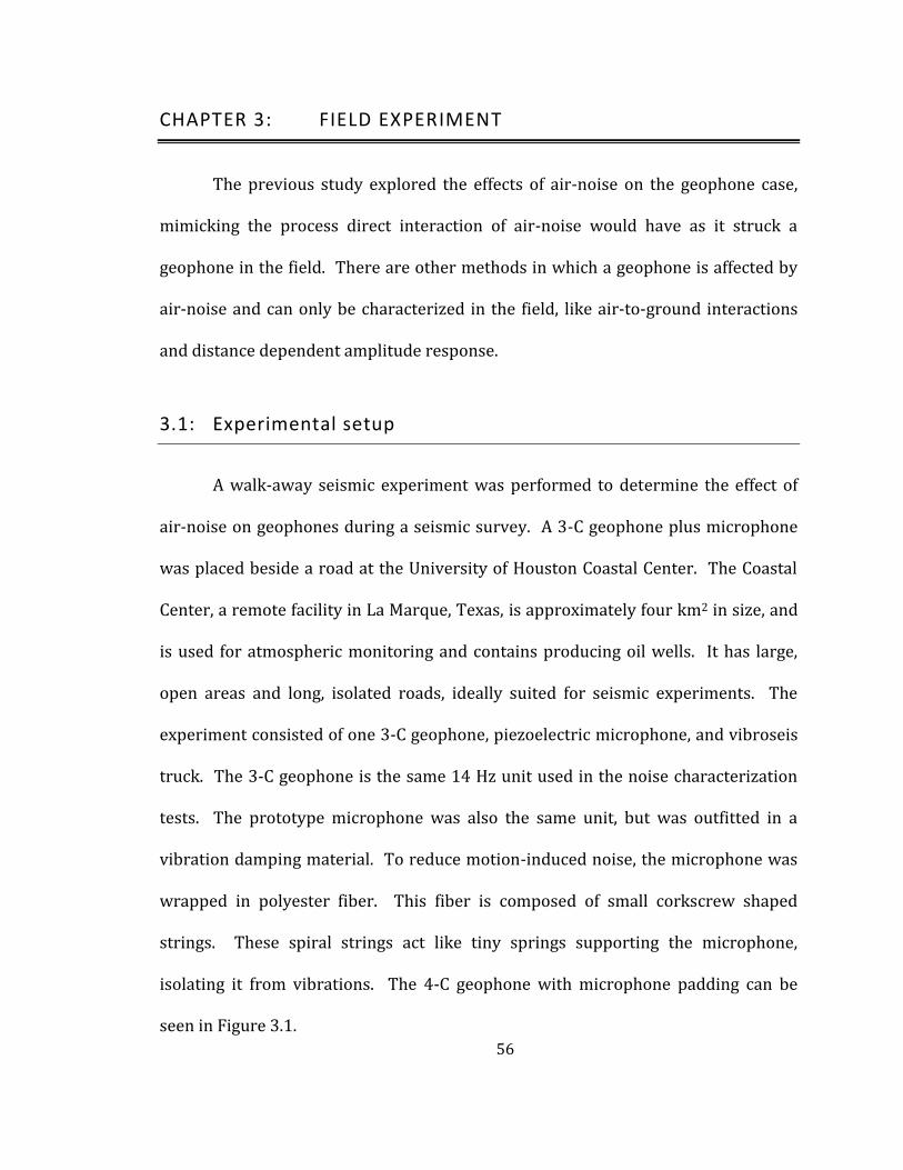
56

CHAPTER 3: FIELD EXPERIMENT

The previous study explored the effects of air-noise on the geophone case,

mimicking the process direct interaction of air-noise would have as it struck a

geophone in the field. There are other methods in which a geophone is affected by

air-noise and can only be characterized in the field, like air-to-ground interactions

and distance dependent amplitude response.

3.1: Experimental setup

A walk-away seismic experiment was performed to determine the effect of

air-noise on geophones during a seismic survey. A 3-C geophone plus microphone

was placed beside a road at the University of Houston Coastal Center. The Coastal

Center, a remote facility in La Marque, Texas, is approximately four km2 in size, and

is used for atmospheric monitoring and contains producing oil wells. It has large,

open areas and long, isolated roads, ideally suited for seismic experiments. The

experiment consisted of one 3-C geophone, piezoelectric microphone, and vibroseis

truck. The 3-C geophone is the same 14 Hz unit used in the noise characterization

tests. The prototype microphone was also the same unit, but was outfitted in a

vibration damping material. To reduce motion-induced noise, the microphone was

wrapped in polyester fiber. This fiber is composed of small corkscrew shaped

strings. These spiral strings act like tiny springs supporting the microphone,

isolating it from vibrations. The 4-C geophone with microphone padding can be

seen in Figure 3.1.

57

The geophone and microphone (4-C geophone) were placed along a dirt road

inside the facility, and the shot line continued down the road. The first shot point

was 2.5 m behind the 4-C geophone and shots were taken every 5 m, to 702.5 m in

front of the 4-C geophone (Figure 3.2). Each shot consisted of a single sweep from

the vibroseis truck, from 15 to 150 Hz over 12 s. Sixteen seconds of uncorrelated

data were recorded for each shot, so that analysis could take place on the raw data.

Figure 3.1: The "pillow-top" vibration isolation system. The piezo microphone is

placed inside a felt pocket, surrounded by polyester fibers. These springy fibers

dampen vibrations that affect the microphone. Shown attached atop a 3-C geophone.

58

Figure 3.2: Survey location and schematic. Satellite imagery of the northern portion

of the UH Coastal Center, near La Marque, Texas. The blue circle shows the

approximate 4-C prototype geophone position, defined as 0 m. The red line indicates

the shot line, from -2.5 m to 702.5 m shot at a 5 m interval.

Imagery source (Google Maps, 2012)

The test site had little cultural noise; i.e. noise created from non-natural

sources such as traffic, construction or other human activities. There was, however,

a large amount of environmental noise, or natural background noise, mostly from

wind. The nearest roads were located approximately 400 and 1000 meters away,

behind a large stand of trees. Audible noise from the roads was occasionally

discernible, but any vehicle-induced ground vibrations were undetectable. The dirt

road on which the experiment took place carried sparse traffic. Shooting was halted

when traffic passed to ensure clean data were acquired. Winds on the day of the

survey ranged from 15 to 25 km/hr. This caused discernible noise in both the

seismic and acoustic records.

59

After the survey, all shot records were combined in a common receiver

gather, to simulate a 700 m, 4-C geophone line. This process allows the

experimentation of noise cancellation along a full seismic record without needing to

make 140 4-C geophones.

3.2: Geophone data analysis

Before analyzing the air-noise data, it is best to define from theory what to

expect. While expectations about transient air-noise response cannot be

determined beforehand, vibrator-induced air-wave is easily characterized. The

majority of the air-wave energy transmits directly through the air. When travelling

across a spread of geophones, this is seen as a linear event, originating at the shot

location, travelling around 345 m/s (dependent on temperature and pressure). The

air-wave will interact with the ground, creating ground-roll and compressional

waves. The conversion to compressional waves occurs across a wide range of

frequencies, and depends on many factors, such as the acoustic impedance of the

weathering layer. The ground-roll conversion only occurs at a single frequency,

which depends on the weathering layer thickness. Any air-wave-induced ground-

roll will be seen as a monofrequency wave-train following any air-noise arrival. The

reverse of these processes occur as well, ground motion will convert to air motion.

Ground roll will couple to monofrequency air-wave, and compressional waves will

convert to air-wave as well. In short, in the seismic record, the linear air-wave

should be easily seen, which should be followed by a monofrequency wave-train.

60

The acoustic record will also show the direct air-wave arrival, and the

monofrequency wave train following it. Microphones may also record the energy

from other compressional seismic-wave arrivals, but recorded evidence of this

process has yet to be published for seismic experiments.

The raw data were correlated in MATLAB for initial analysis. The correlated

geophone gathers can be seen in Figure 3.3, Figure 3.4, and Figure 3.5. Even with

the high levels of wind noise, and only single vertical fold, the geophone collected

good data. Using only 500 ms AGC, reflectors can be seen deeper than 1000 ms on

the vertical component. The crossline component detected reflectors down to 650

ms, but the inline component only detected the shallowest reflectors, below 400 ms.

The head-wave response is very strong on the vertical and crossline components,

but weaker on the inline component. There appears to be only a single visible

refracting layer with a velocity of 1750 m/s. This refracting layer is also very

shallow, evidenced by the lack of a visible direct arrival at near offsets. The weaker

recordings by the inline component, compared to the crossline component, are of

interest. Typically, the inline component should see a strong head-wave response

while the crossline component is weaker. The nearby road could cause this. The

high-velocity, well-compacted roadbed may bend incoming arrivals toward the

crossline direction.

The air-wave response from the geophone is much more atypical. According

to the sensitivity diagrams for the 3-C geophone, the vertical and inline components

should show a strong response to air-wave, while the crossline component response

61

Figure 3.3: Vertical component correlated shot gather. Displayed using 500 ms AGC,

showing the first 2.5 s of the record. Note the very weak air-wave.

62

Figure 3.4: Crossline component correlated shot gather. Displayed using 500 ms AGC,

showing the first 2.5 s of the record.

63

Figure 3.5: Inline component correlated shot gather. Displayed using 500 ms AGC,

showing the first 2.5 s of the record. Note the strong air-wave. There is also shear-

wave refractions located beneath the air-wave.

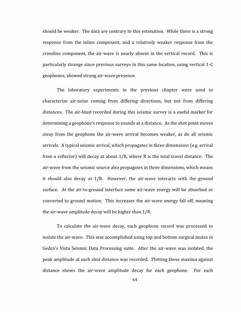
64

should be weaker. The data are contrary to this estimation. While there is a strong

response from the inline component, and a relatively weaker response from the

crossline component, the air-wave is nearly absent in the vertical record. This is

particularly strange since previous surveys in this same location, using vertical 1-C

geophones, showed strong air-wave presence.

The laboratory experiments in the previous chapter were used to

characterize air-noise coming from differing directions, but not from differing

distances. The air-blast recorded during this seismic survey is a useful marker for

determining a geophone’s response to sounds at a distance. As the shot point moves

away from the geophone the air-wave arrival becomes weaker, as do all seismic

arrivals. A typical seismic arrival, which propagates in three dimensions (e.g. arrival

from a reflector) will decay at about 1/R, where R is the total travel distance. The

air-wave from the seismic source also propagates in three dimensions, which means

it should also decay at 1/R. However, the air-wave interacts with the ground

surface. At the air-to-ground interface some air-wave energy will be absorbed or

converted to ground motion. This increases the air-wave energy fall off, meaning

the air-wave amplitude decay will be higher than 1/R.

To calculate the air-wave decay, each geophone record was processed to

isolate the air-wave. This was accomplished using top and bottom surgical mutes in

Gedco’s Vista Seismic Data Processing suite. After the air-wave was isolated, the

peak amplitude at each shot distance was recorded. Plotting these maxima against

distance shows the air-wave amplitude decay for each geophone. For each

65

geophone component, the amplitudes from the first 50 m were discarded because

they are affected by near offset effects. All data past 500 m was also discarded

because the air-wave response was obscured by background noise. A power trend

line was fit to the data from each geophone component to determine the amplitude

decay. The data for each component, with trend lines, are in Figure 3.6. None of the

air-wave arrivals had a decay rate of 1/R. The vertical component decayed at

1/R^1.8, while the inline components decayed at 1/R^1.4, and the crossline

component decayed at 1/R^1.1. This indicated that each geophone element

behaves differently to the same air-wave that passes the geophone.

66

Figure 3.6: Geophone amplitude decay comparison for the air-wave arrival. The

vertical component amplitude decays much faster than the horizontal components.

67

3.3: Microphone data analysis

The microphone, as it should, shows a large air-wave presence across the

entire spread (Figure 3.7). In its entirety the air-wave lasts for 200 ms in the near

field and 150 ms in the far field. The record shows the constant presence of

electrical cross-talk with the pilot channel. This is evidenced by the persistent high

amplitude event between 0 and 75 ms. This crosstalk occurs because the

microphone was not specifically designed to connect with this recording system. An

optimized design would eliminate this effect. The peak crosstalk magnitude on the

microphone is 1.3*1011, compared to 2.5*1015 for the auto-correlated pilot trace,

giving a crosstalk ratio of 19000:1 or -86dB from pilot to microphone.

The air-wave amplitude decay was analyzed in the same manner as the

geophone. The air-wave was isolated in the microphone record using surgical

mutes, and the maximum amplitude at each shot point was recorded. The first 50 m

of data were discarded to ignore near-field effects, but the rest of the data (out to

702.5 m) were used for analysis because the air-wave remained strong across the

entire shot spread. A plot of the data with a power trend line is shown in Figure 3.8.

Like the geophone, the microphone amplitude does not decay at 1/R; it decays at

1/R^1.4. The difference in amplitude decay between the microphone and each

geophone component is important and must be taken into consideration when

designing an air-wave filter.

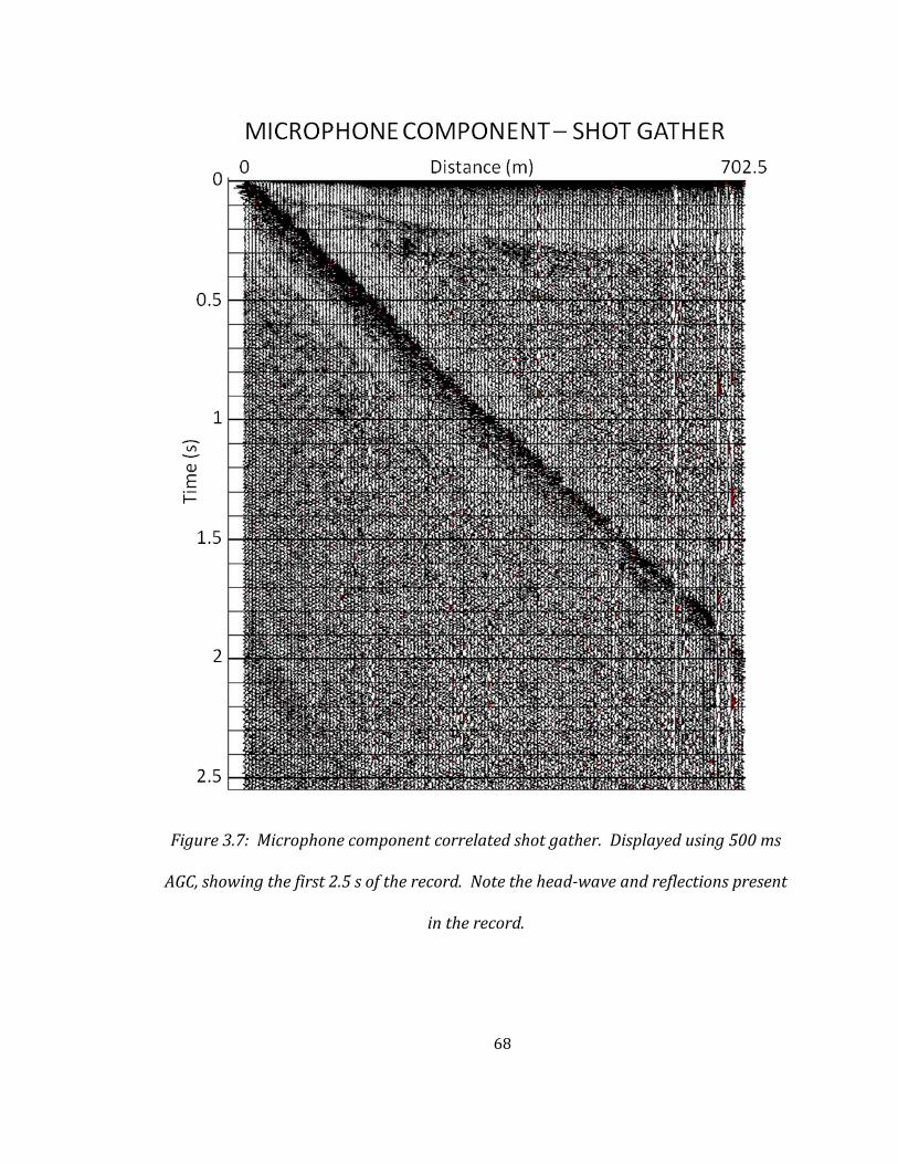
68

Figure 3.7: Microphone component correlated shot gather. Displayed using 500 ms

AGC, showing the first 2.5 s of the record. Note the head-wave and reflections present

in the record.

69

Figure 3.8: Microphone recorded air-wave amplitude decay. The microphone decay

rate is similar to the horizontal geophone components.

There are other visible events in the microphone record, consisting of a

series of monofrequency arrivals, which coincide with the head wave, and

uppermost reflections. One of three things could cause these peculiar events:

electrical crosstalk with the adjacent inline geophone component, physical motion

of the microphone converting to spurious recorded voltage, or it could be the record

of ground-to-air converted seismic energy. If these events were caused by electrical

crosstalk, it should have a similar crosstalk ratio when compared to the pilot-

channel crosstalk. The peak microphone head-wave response is 2.2*1010 whereas

the inline geophone component only has a peak magnitude of 1.1*1010. This gives

70

an inline-to-microphone crosstalk ratio of 1:2 or +6 dB. This is much too large for

electrical crosstalk. In fact, it would suggest microphone-to-inline crosstalk since

the microphone magnitude is greater. Even the vertical geophone component, with

the strongest head wave response, has a peak magnitude of 1.6*1011. This gives a

vertical-to-microphone crosstalk ratio of 1.45:1 or -3 dB. Therefore, these events

are most likely not caused by crosstalk.

The microphone is constructed of two piezoelectric discs glued on opposite

sides of a ring. Each piezo-element is inherently susceptible to noise induced by

motion of the element. However, the elements are mounted in opposing directions.

This means, a motion that induces a positive voltage on one element produces a

negative voltage on the other element. When wired in series these voltages

effectively cancel out. This process is not perfect, so small voltage anomalies may

arise when the microphone is moved, shaken, or vibrated. To reduce excess motion

of the microphone, it was decoupled from the geophone. This was achieved by

wrapping the microphone loosely with polyester fiber called poly-fill. When used in

small amounts, it is acoustically transparent. The poly-fill fibers consist of small

spirals of polyester, which act as a spring, absorbing vibration. If, after decoupling,

the microphone were still moved by vibrations of the geophone, a visible response

should be seen in the microphone record for each seismic event in the geophone

record. The only events that correlate between microphone and geophone are the

head-wave and uppermost reflections. Furthermore, any mechanical coupling

recorded by the microphone should have similar frequency content when compared

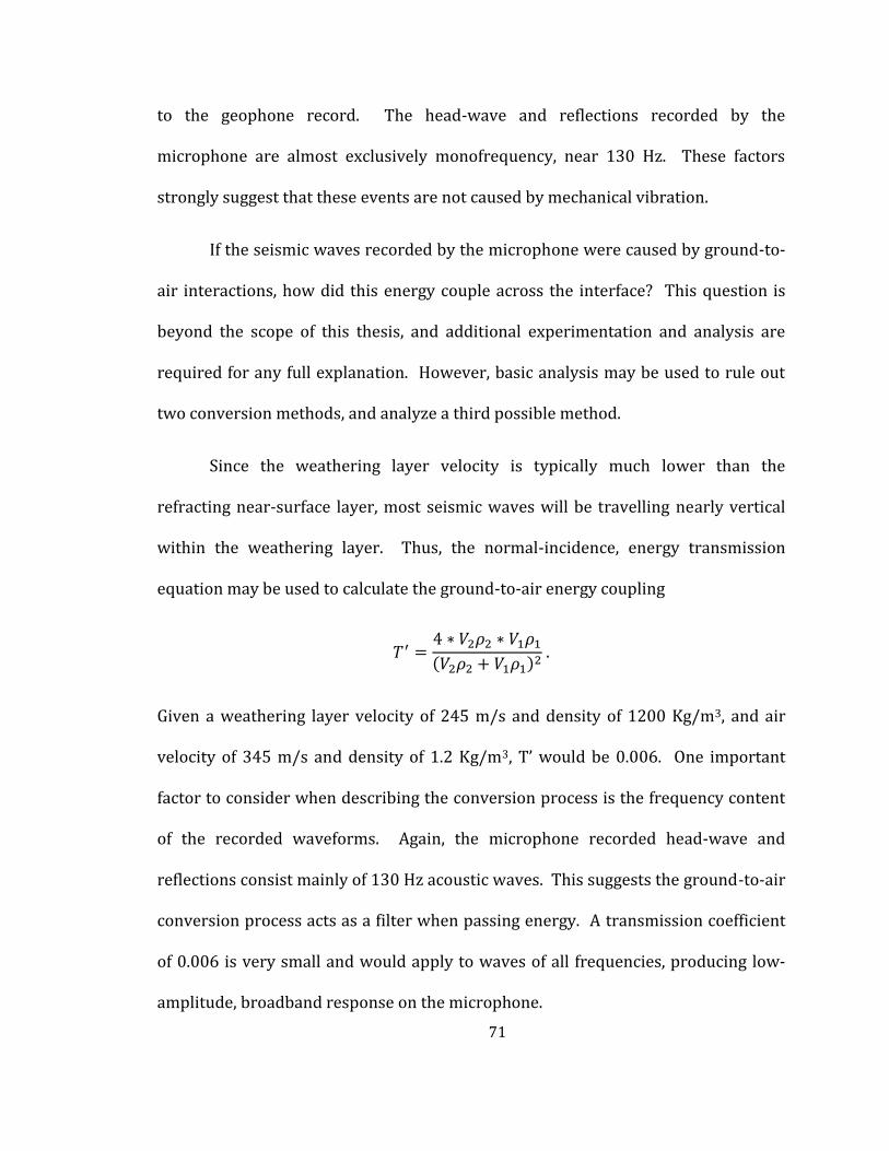
71

to the geophone record. The head-wave and reflections recorded by the

microphone are almost exclusively monofrequency, near 130 Hz. These factors

strongly suggest that these events are not caused by mechanical vibration.

If the seismic waves recorded by the microphone were caused by ground-to-

air interactions, how did this energy couple across the interface? This question is

beyond the scope of this thesis, and additional experimentation and analysis are

required for any full explanation. However, basic analysis may be used to rule out

two conversion methods, and analyze a third possible method.

Since the weathering layer velocity is typically much lower than the

refracting near-surface layer, most seismic waves will be travelling nearly vertical

within the weathering layer. Thus, the normal-incidence, energy transmission

equation may be used to calculate the ground-to-air energy coupling

Given a weathering layer velocity of 245 m/s and density of 1200 Kg/m3, and air

velocity of 345 m/s and density of 1.2 Kg/m3, T’ would be 0.006. One important

factor to consider when describing the conversion process is the frequency content

of the recorded waveforms. Again, the microphone recorded head-wave and

reflections consist mainly of 130 Hz acoustic waves. This suggests the ground-to-air

conversion process acts as a filter when passing energy. A transmission coefficient

of 0.006 is very small and would apply to waves of all frequencies, producing low-

amplitude, broadband response on the microphone.

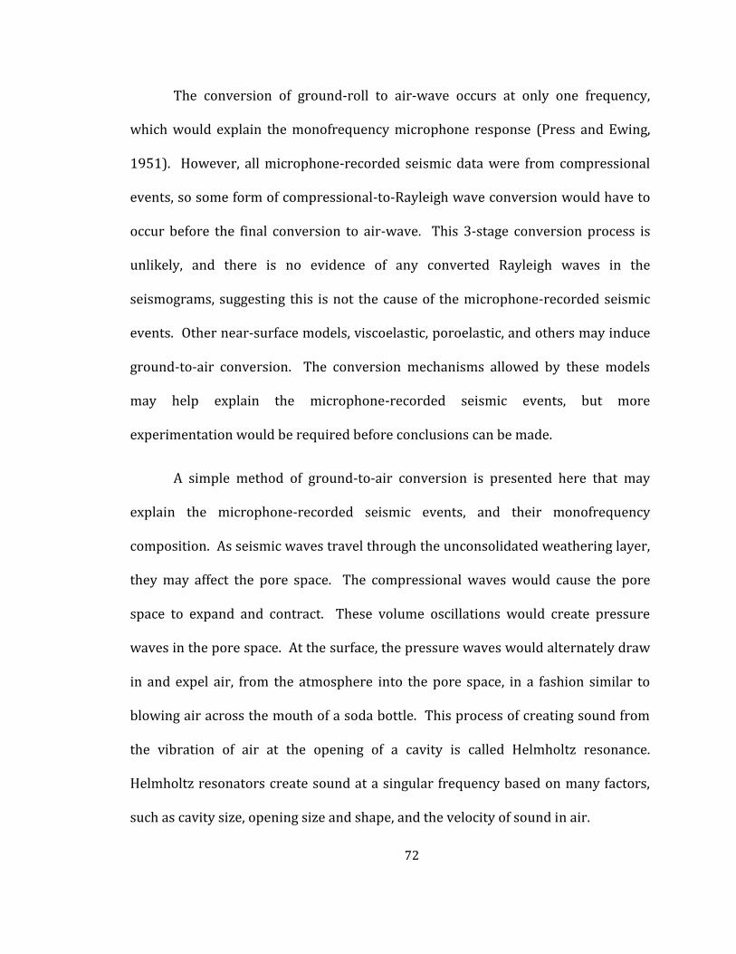
72

The conversion of ground-roll to air-wave occurs at only one frequency,

which would explain the monofrequency microphone response (Press and Ewing,

1951). However, all microphone-recorded seismic data were from compressional

events, so some form of compressional-to-Rayleigh wave conversion would have to

occur before the final conversion to air-wave. This 3-stage conversion process is

unlikely, and there is no evidence of any converted Rayleigh waves in the

seismograms, suggesting this is not the cause of the microphone-recorded seismic

events. Other near-surface models, viscoelastic, poroelastic, and others may induce

ground-to-air conversion. The conversion mechanisms allowed by these models

may help explain the microphone-recorded seismic events, but more

experimentation would be required before conclusions can be made.

A simple method of ground-to-air conversion is presented here that may

explain the microphone-recorded seismic events, and their monofrequency

composition. As seismic waves travel through the unconsolidated weathering layer,

they may affect the pore space. The compressional waves would cause the pore

space to expand and contract. These volume oscillations would create pressure

waves in the pore space. At the surface, the pressure waves would alternately draw

in and expel air, from the atmosphere into the pore space, in a fashion similar to

blowing air across the mouth of a soda bottle. This process of creating sound from

the vibration of air at the opening of a cavity is called Helmholtz resonance.

Helmholtz resonators create sound at a singular frequency based on many factors,

such as cavity size, opening size and shape, and the velocity of sound in air.

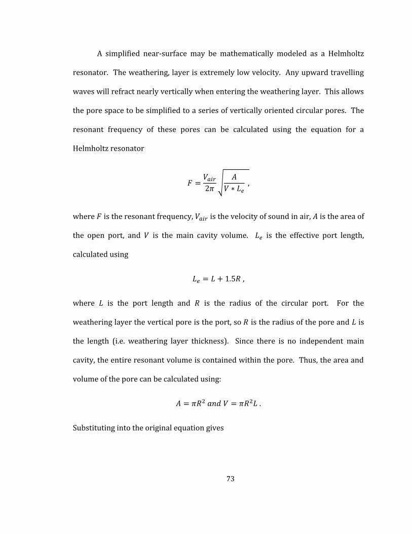
73

A simplified near-surface may be mathematically modeled as a Helmholtz

resonator. The weathering, layer is extremely low velocity. Any upward travelling

waves will refract nearly vertically when entering the weathering layer. This allows

the pore space to be simplified to a series of vertically oriented circular pores. The

resonant frequency of these pores can be calculated using the equation for a

Helmholtz resonator

√

where is the resonant frequency, is the velocity of sound in air, is the area of

the open port, and is the main cavity volume. is the effective port length,

calculated using

where is the port length and is the radius of the circular port. For the

weathering layer the vertical pore is the port, so is the radius of the pore and is

the length (i.e. weathering layer thickness). Since there is no independent main

cavity, the entire resonant volume is contained within the pore. Thus, the area and

volume of the pore can be calculated using:

Substituting into the original equation gives

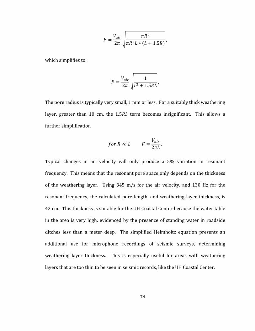
74

√

which simplifies to:

√

The pore radius is typically very small, 1 mm or less. For a suitably thick weathering

layer, greater than 10 cm, the term becomes insignificant. This allows a

further simplification

Typical changes in air velocity will only produce a 5% variation in resonant

frequency. This means that the resonant pore space only depends on the thickness

of the weathering layer. Using 345 m/s for the air velocity, and 130 Hz for the

resonant frequency, the calculated pore length, and weathering layer thickness, is

42 cm. This thickness is suitable for the UH Coastal Center because the water table

in the area is very high, evidenced by the presence of standing water in roadside

ditches less than a meter deep. The simplified Helmholtz equation presents an

additional use for microphone recordings of seismic surveys, determining

weathering layer thickness. This is especially useful for areas with weathering

layers that are too thin to be seen in seismic records, like the UH Coastal Center.

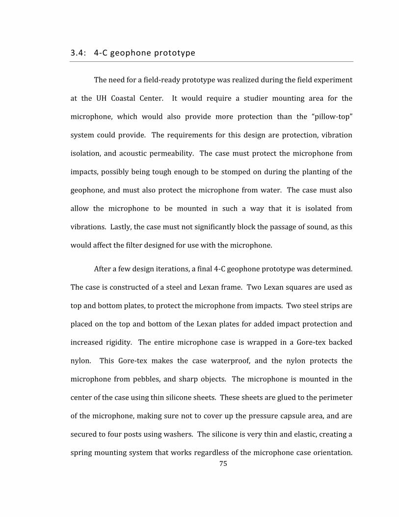
75

3.4: 4-C geophone prototype

The need for a field-ready prototype was realized during the field experiment

at the UH Coastal Center. It would require a studier mounting area for the

microphone, which would also provide more protection than the “pillow-top”

system could provide. The requirements for this design are protection, vibration

isolation, and acoustic permeability. The case must protect the microphone from

impacts, possibly being tough enough to be stomped on during the planting of the

geophone, and must also protect the microphone from water. The case must also

allow the microphone to be mounted in such a way that it is isolated from

vibrations. Lastly, the case must not significantly block the passage of sound, as this

would affect the filter designed for use with the microphone.

After a few design iterations, a final 4-C geophone prototype was determined.

The case is constructed of a steel and Lexan frame. Two Lexan squares are used as

top and bottom plates, to protect the microphone from impacts. Two steel strips are

placed on the top and bottom of the Lexan plates for added impact protection and

increased rigidity. The entire microphone case is wrapped in a Gore-tex backed

nylon. This Gore-tex makes the case waterproof, and the nylon protects the

microphone from pebbles, and sharp objects. The microphone is mounted in the

center of the case using thin silicone sheets. These sheets are glued to the perimeter

of the microphone, making sure not to cover up the pressure capsule area, and are

secured to four posts using washers. The silicone is very thin and elastic, creating a

spring mounting system that works regardless of the microphone case orientation.

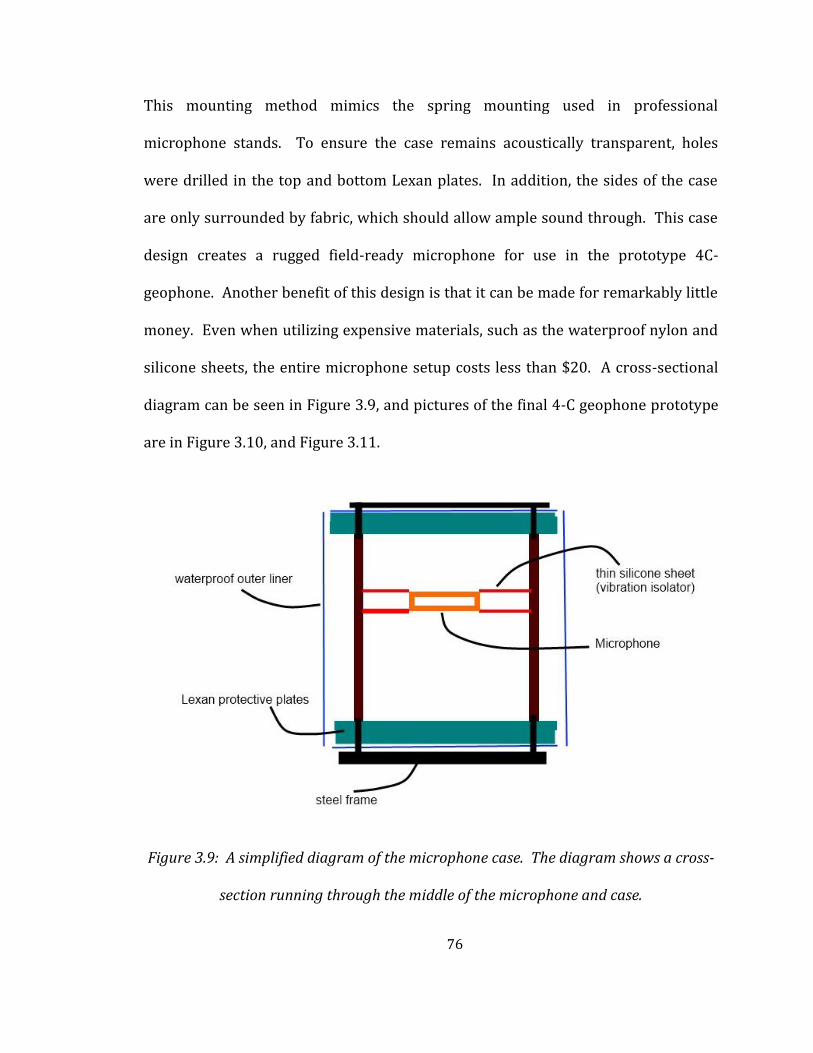
76

This mounting method mimics the spring mounting used in professional

microphone stands. To ensure the case remains acoustically transparent, holes

were drilled in the top and bottom Lexan plates. In addition, the sides of the case

are only surrounded by fabric, which should allow ample sound through. This case

design creates a rugged field-ready microphone for use in the prototype 4C-

geophone. Another benefit of this design is that it can be made for remarkably little

money. Even when utilizing expensive materials, such as the waterproof nylon and

silicone sheets, the entire microphone setup costs less than $20. A cross-sectional

diagram can be seen in Figure 3.9, and pictures of the final 4-C geophone prototype

are in Figure 3.10, and Figure 3.11.

Figure 3.9: A simplified diagram of the microphone case. The diagram shows a cross-

section running through the middle of the microphone and case.

77

Figure 3.10: The finished microphone case. The steel plates on top allow the

microphone to be stomped on, while the blue nylon keeps the microphone dry.

Figure 3.11: The finished prototype 4-C geophone, sitting atop a 3-C geophone in the

field.

78

3.5: Conclusion

The presence of head-waves and reflections in the microphone record is

quite surprising. This phenomenon, thus far, has been unseen in published

research. That is why extreme care was taken to consider other possible factors

before suggesting these seismic events were recorded from ground-to-air converted

energy. Electrical crosstalk was ruled out, due to the large amplitude of the events,

relative to geophone records. Mechanical coupling is also very unlikely, due to the

narrowband response of the events and care taken to decouple the microphone

from ground motion. This leaves ground-to-air conversion as the explanation for

these events. Helmholtz resonance of the near surface pores effectively explains the

ground-to-air conversion causing the microphone-recorded seismic events. This

resonance depends mainly on weathering-layer depth, which for the UH Coastal

Center is defined by the water table. Calculating this depth from Helmholtz

resonance agrees with field observations of a shallow water table, supporting this

simplified conversion method. However, there are many other ways to convert

seismic waves to atmospheric waves, and full testing of each method needs to be

made before a full conclusion may be drawn.

79

CHAPTER 4: NOISE-CANCELLING FILTER

The previous chapters covered the characterization of how noise affects

geophones, and how microphones behave in the field. They are:

1. The geophone is directionally sensitive to noise

2. Each geophone component has a different directional sensitivity

3. The geophone-microphone amplitude transfer function is dependent on

frequency and incident sound angle

4. The geophone-microphone phase transfer function is dependent on

frequency and incident sound angle.

5. Each geophone component’s amplitude decay curve differs from each

other and the microphone.

The information gained from these characterizations helps define the structure and

process of the air-noise filter.

4.1: Filter design

A geophone responds differently to sounds coming from differing directions.

This means that the air-noise filter must be able to detect an incoming sound’s

direction. Furthermore, each geophone component responds differently to sounds

coming from the same direction, so individual filters must be used for each

geophone component. The geophone’s noise response not only varies with

direction but distance as well. Thus, the filter must also determine the distance the

80

sound has travelled before hitting the geophone. Fortunately, a few behaviors of the

geophone-microphone system may be exploited to greatly simplify the filtering

process.

Because the sound phase varies between the microphone and geophone,

their phases must be rectified before filtering. This solves the problem of

determining any particular sound’s direction. The filter can use the amplitude from

the microphone with the phase from the geophone to create an effectively phase

shifted microphone signal. This step not only accounts for the differing incoming

sound directions, but the geophone-microphone phase transfer function as well.

One weakness of this solution is that it will phase shift all data from the microphone,

including background noise. For example, in windy environments, the wind noise

will be phase shifted to match the geophone, possibly affecting geophone data. This

factor can be controlled by housing the microphone in a protective case, which could

block wind yet still pass sound.

The amplitude kernel is the relative air-noise response strength of the

geophone compared to the microphone. It cannot be calculated during the filtering

process because the filter cannot separate air-noise from seismic signal on the

geophone component. Thus, it must be hard coded in the filter. An amplitude

kernel is calculated by dividing the maximum Gabor amplitude from the geophone

by the maximum from the microphone, for every frequency. This is performed

using the equation,

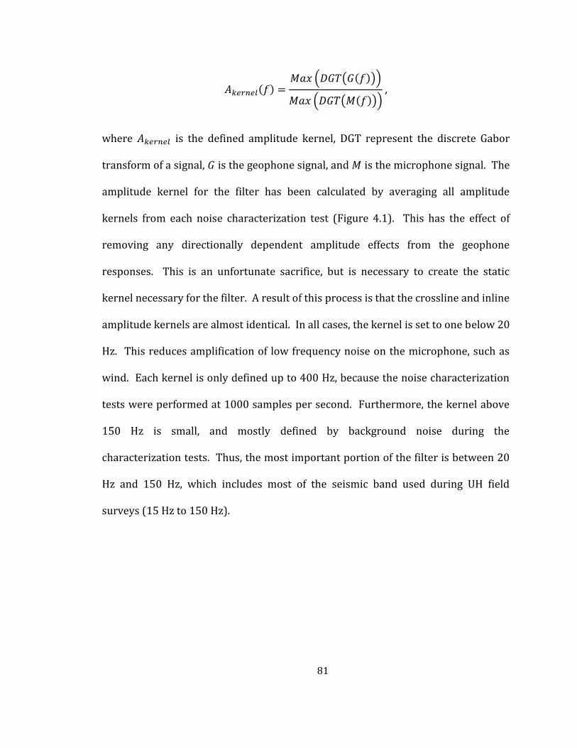
81

( ( ))

( ( ))

where is the defined amplitude kernel, DGT represent the discrete Gabor

transform of a signal, is the geophone signal, and is the microphone signal. The

amplitude kernel for the filter has been calculated by averaging all amplitude

kernels from each noise characterization test (Figure 4.1). This has the effect of

removing any directionally dependent amplitude effects from the geophone

responses. This is an unfortunate sacrifice, but is necessary to create the static

kernel necessary for the filter. A result of this process is that the crossline and inline

amplitude kernels are almost identical. In all cases, the kernel is set to one below 20

Hz. This reduces amplification of low frequency noise on the microphone, such as

wind. Each kernel is only defined up to 400 Hz, because the noise characterization

tests were performed at 1000 samples per second. Furthermore, the kernel above

150 Hz is small, and mostly defined by background noise during the

characterization tests. Thus, the most important portion of the filter is between 20

Hz and 150 Hz, which includes most of the seismic band used during UH field

surveys (15 Hz to 150 Hz).

82

Figure 4.1: Amplitude kernels for each geophone component. The crossline and inline

kernels are almost identical. This is the result of averaging kernels from multiple

directions, removing directional dependency from kernel response.

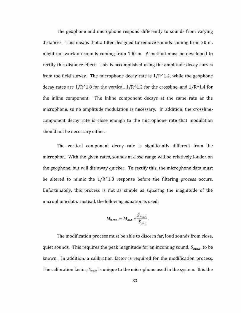
83

The geophone and microphone respond differently to sounds from varying

distances. This means that a filter designed to remove sounds coming from 20 m,

might not work on sounds coming from 100 m. A method must be developed to

rectify this distance effect. This is accomplished using the amplitude decay curves

from the field survey. The microphone decay rate is 1/R^1.4, while the geophone

decay rates are 1/R^1.8 for the vertical, 1/R^1.2 for the crossline, and 1/R^1.4 for

the inline component. The Inline component decays at the same rate as the

microphone, so no amplitude modulation is necessary. In addition, the crossline-

component decay rate is close enough to the microphone rate that modulation

should not be necessary either.

The vertical component decay rate is significantly different from the

microphon. With the given rates, sounds at close range will be relatively louder on

the geophone, but will die away quicker. To rectify this, the microphone data must

be altered to mimic the 1/R^1.8 response before the filtering process occurs.

Unfortunately, this process is not as simple as squaring the magnitude of the

microphone data. Instead, the following equation is used:

The modification process must be able to discern far, loud sounds from close,

quiet sounds. This requires the peak magnitude for an incoming sound, , to be

known. In addition, a calibration factor is required for the modification process.

The calibration factor, , is unique to the microphone used in the system. It is the

84

peak amplitude, recorded by the microphone, of a vibroseis sweep 8 m away. Eight

meters, was chosen as the calibration distance because it is the “crossover point” for

the microphone-geophone amplitude relation. Sounds closer than 8 m away are

relatively louder on the geophone, and sounds further than 8 m are relatively louder

on the microphone. Thus, sounds closer than this distance must be magnified in

microphone records while sounds further than this must be diminished. The peak

incoming sound magnitude, divided by the calibration factor, effectively performs

this transformation. When multiplied by the original microphone signal, a

new microphone signal, is created with appropriately magnified or

diminished sounds, based on the perceived sound’s distance. This gives the

microphone a pseudo 1/R^2 response, which is suitably matched to the geophone

decay rate for the filter process to work effectively.

Each of the previous pieces fit together to make the complete air-noise filter.

From start to finish, the filter works in the following way. An incoming sound is

detected by the microphone and geophone, and is digitally sampled. The sample is

triplicated for use on each geophone component. The sample bound for the vertical

component is modified using a scaling factor determined by the maximum previous

amplitude recorded by the microphone. Using the current time sample and the

previous 127 samples, a frequency spectrum is calculated for the microphone,

vertical, crossline, and inline components. The magnitude of the microphone

spectrum, and the phase for each geophone component, are calculated. Using

microphone magnitude and the three geophone phases, a new spectrum is created

85

called the noise estimate spectrum. These spectra mimic what the geophone air-

noise response should be. The spectra are transformed back to the time domain,

creating the noise estimate signal. The data point that corresponds to the current

time sample is then subtracted from the corresponding geophone component. This

removes the expected air-noise effect from the geophone creating “clean” geophone

outputs. A diagram summarizing this process is in Figure 4.2, and the complete

filtering program is located in Appendix A.

This program has been run on uncorrelated seismic data from the UH Coastal

Center survey, to test its effectiveness and ability to run in real-time. The filter’s

effectiveness will be discussed in the next section, but a few statements can be made

about its speed. It can process 16 s of uncorrelated data in 18 s. This is not true

real-time processing, but the original program has not been optimized for speed and

had significant overhead. The program runs on data already acquired, so it is

merely simulating the real-time process of data acquisition. Each shot point is run

separately in the program, and must be loaded from SEG Y files. Time samples are

passed to the real-time filter, one at a time, simulating the live filtering process.

After removing this overhead, and with minimal optimizations, this program should

be able to run in real-time.

86

Figure 4.2: Filter process diagram. Data inputs are amplitude modulated for distance,

then transformed to the frequency-domain. Three amplitude kernels are applied to

the microphone spectrum to estimate the magnitude of noise for each geophone

component. These noise-magnitude estimates are combined with the corresponding

geophone phase to create noise-spectra estimates. Each noise spectrum is converted

back to the time-domain, where the newly created noise signal is subtracted from the

geophone signal. The post-acquisition filter includes an additional step; it applies a

windowing function to the noise signal to isolate the air-noise for improved precision

during air-noise removal.

87

4.2: Filter results

The data acquired at the UH Coastal Center has been processed through the

real-time filter. Before discussing the results, a rubric should be created to evaluate

the effectiveness of the filter. Primarily, the filter should remove a significant

portion of the air-wave from the data. The filter should also not affect seismic

information, such as the head-wave or reflections. Ground roll could possibly be

affected, depending on how much ground-roll-coupled air-wave is present. The

largest source of air-noise in the seismic records is the air-wave from the vibroseis

truck. The filtering of this event will serve as the benchmark for the filter. The real-

time filter results will be compared to other basic filtering methods, including a

high-cut Ormsby filter, and FK-domain velocity filter. The high-cut Ormsby filter is a

simple method of removing noise from seismograms, typically used for quality

control checking in the field. The least restrictive filter that was able to remove the

air-noise had high-cut corners at 90 Hz and 100 Hz. The next filter, a FK-domain

velocity filter is typically used as a first attempt to remove noise during processing.

To remove air-wave, a rejection zone is highlighted in the FK spectrum around

events traveling 345 m/s. This method is only partially effective because air-wave is

usually spatially aliased. Lastly, a post-processing version of the real-time filter will

be shown. For each component, the air-wave in the noise-estimate signal is isolated,

and the result is subtracted from the raw data. This filter shows how microphone

data may be used to remove noise post-acquisition, and in the time domain.

88

4.2.1: Vertical component

The vertical component will be the first result shown, mostly because it is the

most common in seismic data. This dataset has the weakest air-wave response, so

any effect the filter has will be subtle. Comparison diagrams of the varying filter

methods are shown in Figure 4.3 and Figure 4.4

Air-wave noise in the original vertical seismogram is very small, so filter

comparison is fairly limited. The most visible presence of air-wave occurs between

1 s and 1.5 s, in the middle of the spread. This is the area of focus for the

comparative discussion. The noise estimate shows a small amount of air-wave, but

there is also seismic data included in the noise estimate. This is partly from the

presence of seismic data in the microphone record, which is the result of ground-to-

air conversion. While this is good for the prospect of seismic exploration using

microphones, it is not beneficial for air-noise filtering. It can be argued that since

there is a true air response to seismic events, the air pressure created is affecting

the geophone as well, and that it should be removed to retrieve true ground

response to the seismic events. The filtering process, however, is not perfect and

seismic event amplitudes may be affected more than just the intended removal of air

effects. Thus, it is best to leave the seismic arrival amplitudes as close to their

original form as possible. There is also the presence of ground-roll in the noise

estimate. This is an error on the part of the filter. The survey site had a large

amount of background noise, mostly from wind, which was picked up by the

89

microphone. This noise has been phase shifted to match the geophone, creating a

false noise estimate by the filter. Fortunately, this false noise is an order of

magnitude smaller than their corresponding signals in the original seismogram.

The real-time filter removes what little air-wave is present in the original

seismogram. Ground-roll, and other seismic effects, are only minimally affected by

the noise removal process. The windowed post-processing filter produces results

very similar to the real-time filter. The air-wave is effectively removed, but any

effects the false noise estimates had in the real-time filter are gone due to the

windowing process. The high-cut filter is also effective at removing air-wave. It has

the added benefit of removing other high-frequency noise making the reflections at

0.5 s and 0.6 s more visible. However, the filter not only removes high-frequency

noise, but data as well. A loss of detail can be seen in the head wave between 0.1 s

and 0.2 s. The FK-domain filter is the only filter that is unsuccessful in removing the

air-wave. The minor presence of air-wave is present between 1 s and 1.5 s. This

filter also affects a linear event, most likely an S-wave refraction, that is present

between 1 s and 1.6 s on the left side of the seismogram. Because there is so little

air-wave present in the seismogram, a definitive best filter cannot be chosen.

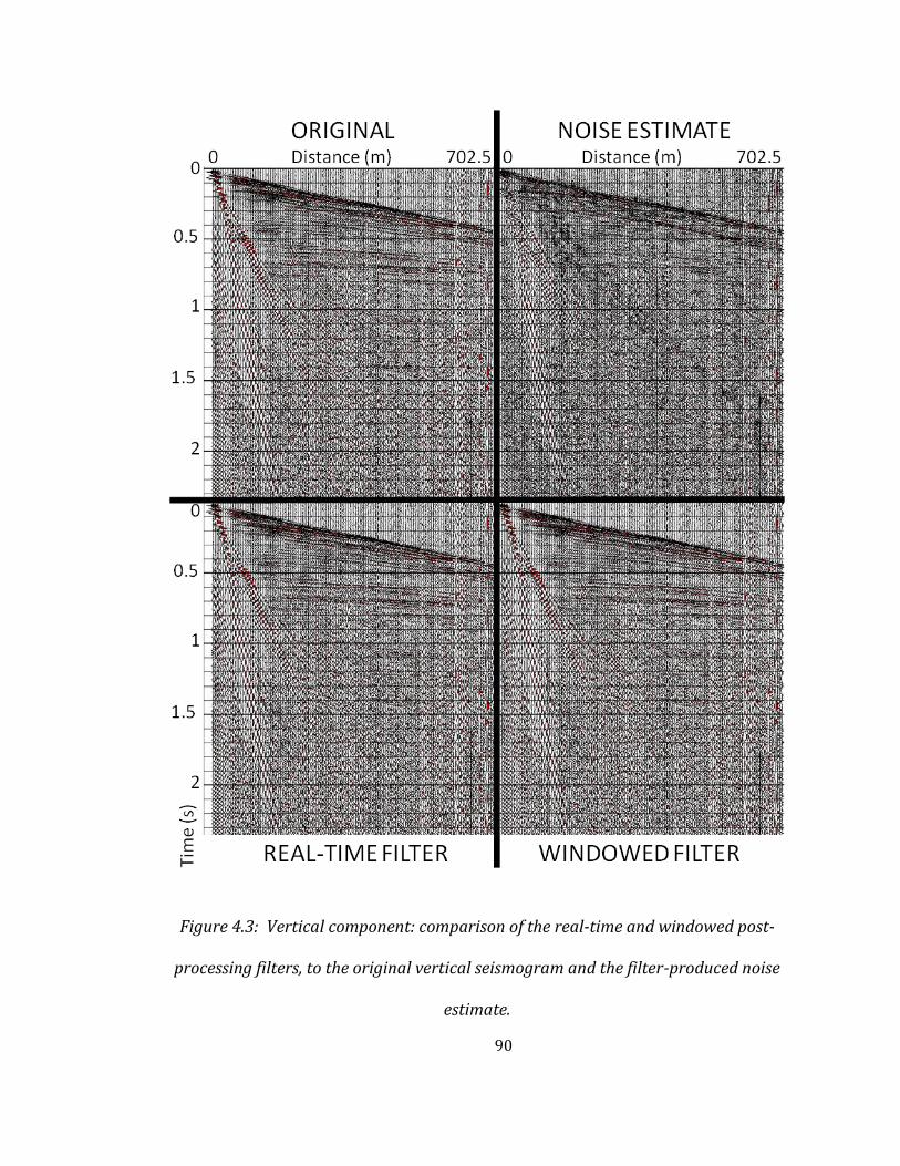
90

Figure 4.3: Vertical component: comparison of the real-time and windowed post-

processing filters, to the original vertical seismogram and the filter-produced noise

estimate.

91

Figure 4.4: Vertical component: comparison of the high-cut and FK-domain velocity

filters, to the original vertical seismogram and the windowed post-processing filter.

92

4.2.2: Crossline component

The crossline component (Figure 4.5 and Figure 4.6) shows a stronger

response to air-wave, which is easily visible from 0.3 s to 1.2 s. After 1.2 s, the air-

wave is still visible, but at diminished amplitudes. The noise estimate from the real-

time filter mirrors the response of the crossline component, visible air-wave out to

1.2 s, with diminished response after. The side effects explored in the vertical

component are also at work here. The presence of seismic arrivals in the

microphone record creates corresponding noise estimates, and ground-roll phase

matching by the wind noise is also visible. The real-time filter removes most of the

air-wave from the crossline component seismogram. The air-wave is now barely

visible before 1.5 s, and completely removed after that. The real-time filter does not

affect the ground-roll very much, but it does affect the head-wave and reflections.

The real-time filter appears to be creating a ghost head-wave 120 ms after the

original arrival. This could be due to artifacts created in the filter. These artifacts

would need to be removed before a field ready filter can be produced. The

windowed filter enjoys the benefits of the real-time filter without the spurious

artifacts. The windowed post-processing filter removes most of the air-wave, to

barely visible levels. This filter is much more accurate than the real-time filter; the

head-wave, reflections, and ground roll are all unaffected due to the windowing

process. The high-cut filter is also effective at removing the air-wave. It does,

however, greatly affect the head wave and near-surface reflections. This is most

prevalent between 0.1 s and 0.3 s. For a near-surface, engineering-scale seismic

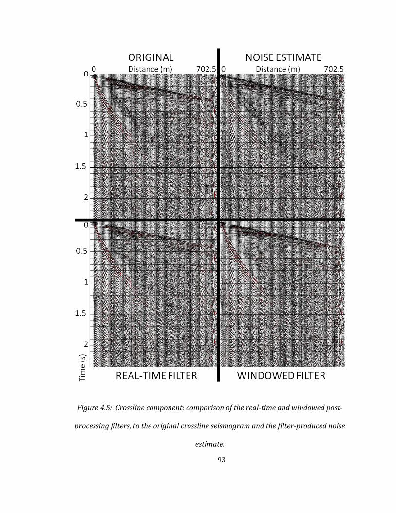
93

Figure 4.5: Crossline component: comparison of the real-time and windowed post-

processing filters, to the original crossline seismogram and the filter-produced noise

estimate.

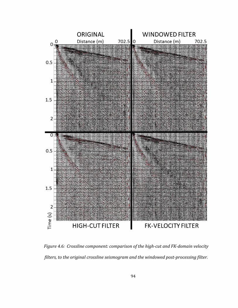
94

Figure 4.6: Crossline component: comparison of the high-cut and FK-domain velocity

filters, to the original crossline seismogram and the windowed post-processing filter.

95

survey this could result in less accurate imaging of subsurface layers. The FK filter

is again unsuccessful at removing air-wave. It only removes a minor portion of the

air-wave. It also removes the S-wave refraction between 0.7 s and 1.2 s. The most

effective filters for this geophone component are the windowed post-processing

filter and the high-cut filter. The windowed filter, does not affect other seismic

arrivals, like the high-cut filter does, making it the more precise filter.

4.2.3: Inline component

The inline geophone component (Figure 4.7 and Figure 4.8) has the strongest

response to air-wave. This is to be expected. As sound travels, the air particles

vibrate radially from their source. At the geophone location, this means the air-

wave is vibrating along the inline direction of the geophone, which is easily visible

across the entire spread. The air-wave noise estimate created by the real-time filter

successfully mimics the inline component. The false ground-roll noise estimate is

present, as well as the microphone-recorded seismic arrivals. The real-time filter

removes most of the air-wave, but at the expense of the reflections and head-wave,

which have been significantly reduced. The ground-roll remains largely unaffected

in the filtering process. The windowed post-processing filter again shows the

benefits of the real-time filter without the side effects. The air-wave is significantly

reduced, and no other seismic information has been seemingly affected. The high-

cut filter is also very effective at removing the air-wave, but again alters the

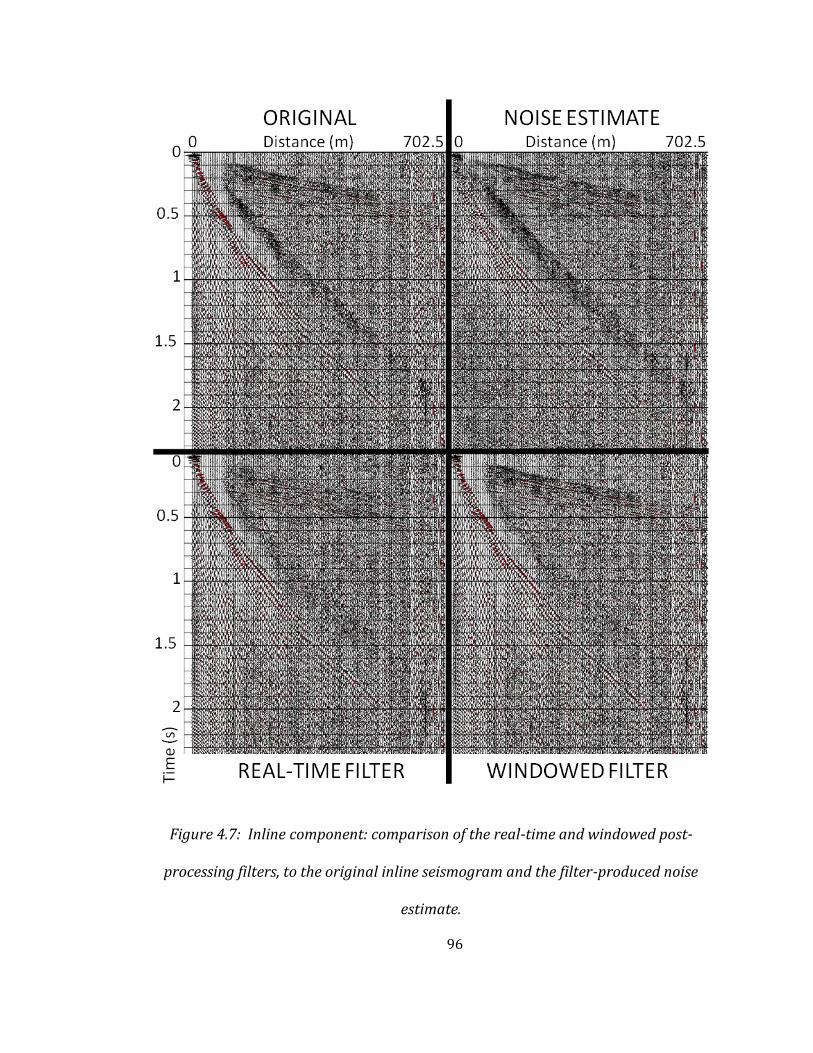
96

Figure 4.7: Inline component: comparison of the real-time and windowed post-

processing filters, to the original inline seismogram and the filter-produced noise

estimate.

97

Figure 4.8: Inline component: comparison of the high-cut and FK-domain velocity

filters, to the original inline seismogram and the windowed post-processing filter.

98

head-wave and reflections. A loss of high frequency content is seen across the entire

head-wave, particularly between 0.15 s and 0.35 s on the left half of the seismogram.

Lastly, the FK-domain filter remains largely ineffective at removing the air-wave.

This filter also removes the S-wave refractions, seen between 0.8 s and 2.0 s. The

conclusions for the inline geophone component are similar to those from the

crossline component. The windowed post-processing filter and the high-cut filter

remain the most effective at removing air-wave, but the windowed filter is more

precise because it does not affect the surrounding seismic events.

4.3: Conclusion

A brief summary of each filter’s effectiveness can be made. The real-time

filter is an interesting prospect; it has the ability to remove air-noise before the

seismograph records it. However, due to the complex relationship between

microphone and geophone the filtering process is not always smooth. Overall, the

real-time filter is effective at removing air-wave, but it also affects other seismic

events. This is partly because these events are also recorded by the microphone,

but also due to an inherent vulnerability in the design. This vulnerability, and the

microphone recorded seismic events can be removed from any noise estimates

using a windowing process around the air-wave. This can only happen as a post-

processing step, removing the live-filtering abilities offered by the original design.

The windowed, post-processing filter was very effective at removing air-wave from

all geophone components, while keeping the remaining seismic events intact. The

99

high-cut filter is the simplest filter in use, and it remains a powerful tool for noise

reduction. It also effectively removes air-wave, but it may not be appropriate for all

seismic experiments. In near-surface studies, high-frequency data are important,

and their removal by a high-cut filter reduces the precision of later measurements.

The last filter used, the FK-domain velocity filter, was the only ineffective filter

tested. It only marginally removed air-wave from the seismograms, yet had

significant effects on other linear events with similar velocities to the air-wave.

In the absence of any microphones, the high-cut filter is recommended for

removing the air-wave, but care should be taken in its application. The windowed

post-processing filter is the best overall option as a filter. Not only is it effective, but

it is very precise, removing only air-wave and not affecting seismic events.

100

CHAPTER 5: DISCUSSION AND CONCLUSIONS

The original intent of this project was to create an air-noise filtering, 4-C

geophone prototype. Initial results from the noise characterization study indicated

a high degree of similarity between microphone and geophone recorded air-noise.

The results from this experiment, combined with some observations from the field

study, led to the development of a real-time air-noise filter. This filter is effective at

removing air-wave from seismic records on all three components. However, the

real-time filter cannot be recommended for field use, at this stage. Another result

from the field survey shows a major flaw in the real-time filtering model, but at the

same time opens great opportunities for microphones in seismic surveys. Real-time,

air-wave filters are ineffective in some cases due to ground-to-air energy

conversion. This conclusion was made because of the presence of head-waves and

reflections in the microphone record, Figure 5.1.

The conversion of seismic-waves to air-waves, as seen in the microphone

record, is not fully understood. One distinguishing trait of these seismic wave

arrivals is they are dominated by a single frequency, near 130 Hz. A few conversion

methods offer partial explanations, only covering the conversion process or the

monofrequency nature of the conversion. Modeling the near surface as a Helmholtz

resonator is the most complete explanation of the microphone-recorded seismic

events. It offers a simplified, albeit incomplete, explanation of the conversion

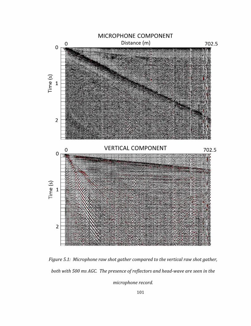
101

Figure 5.1: Microphone raw shot gather compared to the vertical raw shot gather,

both with 500 ms AGC. The presence of reflectors and head-wave are seen in the

microphone record.

102

process, but fully explains the bandpass filtering effect. Furthermore, using the near

surface as a resonator allows for the calculation of the weathering layer depth.

Simplifying the Helmholtz equation, for use with the simplified model, results in the

following conversion from resonant-frequency to weathering-layer depth:

,

where is the speed of sound in air, which is fairly constant, is the depth of the

weathering layer, and is the resonant frequency of the weathering glayer. Using

m/s, , and solving for the weathering layer gives a depth of

42 cm. This is in general agreement with field observations. At the UH Coastal

Center the water table is very shallow, and defines the bottom of the weathering

layer. Standing water was seen in roadside ditches near the survey site indicating a

very shallow weathering layer.

This effect does not happen everywhere, as the weathering layer deepens the

resonant frequency drops. When the weathering layer is 3 m thick the resonant

frequency drops to 18 Hz, and a weathering layer 5 m thick would resonate at 11 Hz.

This means that regions with relatively deep weathering layers might not

necessarily couple to the atmosphere. In places like this, the real-time filter will

work very well, and would be highly recommended for the removal of air-wave.

Areas with shallow weathering layers are still able to utilize microphone records to

remove air-noise, the process only need happen in a different manner. If

microphone data are recorded during a seismic survey, they may easily be used to

103

remove air-wave from seismic records during processing. If the microphone

records contain seismic information, the air-wave can be isolated using surgical

mutes. After this point, the real-time filtering method can be applied using the

modified microphone records to remove air-wave without affecting seismic arrivals.

This is the process which is recommended for the UH Coastal Center, the results of

which can be seen in Figure 5.2.

In conclusion, while this study may not have been a straightforward process

in creating a real-time filter, it has been nonetheless educational. The recordings of

seismic events by the microphone are unique and offer insight into air-ground

interactions. In addition, the filter developed here could be used in real-time (near-

surface conditions permitting), or as a processing step in any conditions.

104

Figure 5.2: Inline component windowed post-processing filter results, both with 500

ms AGC. The filter removes most of the air-wave, without affecting any seismic

arrivals.

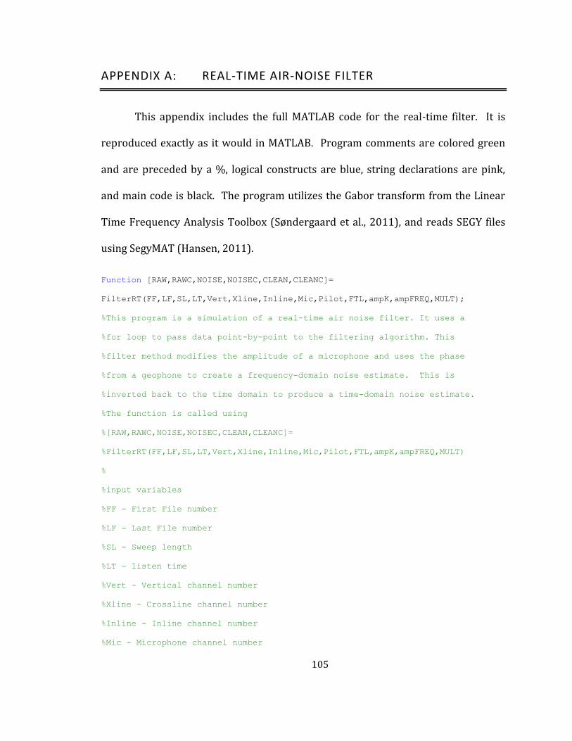
105

APPENDIX A: REAL-TIME AIR-NOISE FILTER

This appendix includes the full MATLAB code for the real-time filter. It is

reproduced exactly as it would in MATLAB. Program comments are colored green

and are preceded by a %, logical constructs are blue, string declarations are pink,

and main code is black. The program utilizes the Gabor transform from the Linear

Time Frequency Analysis Toolbox (Søndergaard et al., 2011), and reads SEGY files

using SegyMAT (Hansen, 2011).

Function [RAW,RAWC,NOISE,NOISEC,CLEAN,CLEANC]=

FilterRT(FF,LF,SL,LT,Vert,Xline,Inline,Mic,Pilot,FTL,ampK,ampFREQ,MULT);

%This program is a simulation of a real-time air noise filter. It uses a

%for loop to pass data point-by-point to the filtering algorithm. This

%filter method modifies the amplitude of a microphone and uses the phase

%from a geophone to create a frequency-domain noise estimate. This is

%inverted back to the time domain to produce a time-domain noise estimate.

%The function is called using

%[RAW,RAWC,NOISE,NOISEC,CLEAN,CLEANC]=

%FilterRT(FF,LF,SL,LT,Vert,Xline,Inline,Mic,Pilot,FTL,ampK,ampFREQ,MULT)

%

%input variables

%FF - First File number

%LF - Last File number

%SL - Sweep length

%LT - listen time

%Vert - Vertical channel number

%Xline - Crossline channel number

%Inline - Inline channel number

%Mic - Microphone channel number

106

%Pilot - pilot channel number

%FTL - Fourier transform length

%ampK - amplitude filter kernel

%ampFREQ – amplitude kernel frequency axis locations

%MULT - final signal adjustment

%

%output variables

%RAW - uncorrelated data from the seismic record

%RAWC - correlated data from the seismic record

%NOISE – uncorrelated noise estimate for each geophone component

%NOISEC – correlated noise estimate for each geophone component

%CLEAN – uncorrelated noise free geophone record

%CLEANC - correlated noise free geophone record

%

%NOTES

%This program works for a single 3-C geophone and microphone combo. The

%input data (released as Data) can be attached to any channel. The output

%data (NOISE and CLEAN)is organized as such: Vertical-CH1, Crossline-CH2,

%Inline-CH3, Microphone-CH4.

%ABOUT THE FILTER

%The filter works by storing the most recent data samples in a buffer. This

%buffer is mirrored and a gaussian window is applied. This action allows

%for th filter to work in real-time. If the buffer was not mirrored the

%filter would work on the central sample, creating a delay of 1/2 the

%Fourier transform length. The microphone data is modified to mimic the

%geophone's amplitude decay (with respect to sound distance). an overview

%of this operation is available within the code. After the symmetric data

%buffer is created a FFT is performed, to convert to the frequency domain.

%In this domain the Microphone is multiplied by each geophones Filter

%Amplitude Kernel. The magnitude of the filtered microphone is used, along

107

%with the phase from the geophone FFT's to create a frequency-domain noise

%estimate. After conversion back to the time-domain, the central sample of

%the noise estimate (which corresponds to the current time) is subtracted

%from the original data. This produces a single geophone signal-sample

%which should be free of air noise. After this the circular data buffers

%are rotated and the filter process is repeated for the next data sample.

%pre allocate variables

NOISE=zeros(16000,3);

CLEAN=zeros(16000,3);

MAXr=zeros(LF-FF+1,1);

Mres=zeros(10,1);

TMPA=FF;

for n=1:LF-FF+1

TMPB=sprintf('%i.sgy',TMPA);

[Data,SegyTraceHeaders,SegyHeader]=ReadSegy(TMPB);

RAW(:,n,:)=Data(:,[Vert Xline Inline Mic Pilot]);

TMPA=TMPA+1;

dt=SegyHeader.time(2)-SegyHeader.time(1);

ts=length(RAW(:,1,1));

xaxisff=(1/dt)*linspace(0,1,2*FTL-1);

Akern=interp1(ampFREQ,ampK,xaxisff,'spline');

%create circular data buffer for FFT

PastV=zeros(FTL,1);

PastX=zeros(FTL,1);

PastI=zeros(FTL,1);

108

PastM=zeros(FTL,1);

%for loop simulates real-time filtering of recorded data

for m=1:length(RAW(:,1,1));

%pass stored data to live variable to mimic real-time filtering.

CdataV=RAW(m,n,1);

CdataX=RAW(m,n,2);

CdataI=RAW(m,n,3);

CdataM=RAW(m,n,4);

%fill new value in data buffer

PastV(FTL)=CdataV;

PastX(FTL)=CdataX;

PastI(FTL)=CdataI;

PastM(FTL)=CdataM;

%Store local peak amplitudes for distance estimation

%local peak amplitudes are picked for each 1000 samples

%they are stored in a buffer for 10000 samples

%the maximum of the local peaks is used in a distance scaling factor

%this factor adjusts the microphone's 1/r response to sound to mimic

%the 1/r^2 response of the geophone. This is calibrated so that sounds

%coming from 8 meters appear as the same ampltude on both Mic and Geop

M(2)=max(abs(PastM));

if rem(m,1000)==0

Mres=circshift(Mres,[-1 0]);

109

Mres(10)=0;

end

if M(2)>=Mres(10)

Mres(10)=M(2);

if M(2)>=max(Mres)

M(1)=M(2);

end

end

if M(2)<max(Mres)

M(1)=max(Mres);

end

if M(2)>MAXr(n)

MAXr(n)=M(2);

end

%creation of symmetric signal for real-time FFT

SymV=PastV;

SymX=PastX;

SymI=PastI;

%microphone amplitudes are scaled by M(1)/8.5362e3 which is

%[max(recent peak amplitudes)]/[peak amplitude of sound from 8m]

%This adjusts the microphone to have a psuedo 1/r^2 response

%This is only used on the Vertical geophone component

SymMV=PastM*(M(1)/8.5362e3);

%The Inline and Xline components don't need affected mic inputs

SymM=PastM;

110

%fill out symmetric signal

SymV(FTL+1:2*FTL-1)=fliplr(SymV(1:FTL-1));

SymX(FTL+1:2*FTL-1)=fliplr(SymX(1:FTL-1));

SymI(FTL+1:2*FTL-1)=fliplr(SymI(1:FTL-1));

SymM(FTL+1:2*FTL-1)=fliplr(SymM(1:FTL-1));

SymMV(FTL+1:2*FTL-1)=fliplr(SymMV(1:FTL-1));

%calculate fft of current data buffer

VftS=fft(gausswin(2*FTL-1).*SymV);

XftS=fft(gausswin(2*FTL-1).*SymX);

IftS=fft(gausswin(2*FTL-1).*SymI);

MftS=fft(gausswin(2*FTL-1).*SymM);

MftSV=fft(gausswin(2*FTL-1).*SymMV);

%calculate phase for each geophone FFT

VphS=angle(VftS);

XphS=angle(XftS);

IphS=angle(IftS);

%apply amplitude filter kernel to microphone FFT

filtV=(abs(MftSV)).*(Akern(:,1));

filtX=(abs(MftS)).*(Akern(:,2));

filtI=(abs(MftS)).*(Akern(:,3));

%filter Vertical geophone trace:

%apply geophone phase to filtered microphone amplitude

%to create Noise estimate FFT

RR=abs(filtV).*cos(VphS);

II=abs(filtV).*sin(VphS);

VftNEWS=complex(RR,II);

111

%IFFT to create local-noise estimate time signal

TMP4=real(ifft(VftNEWS));

TMP6=TMP4(1:2*FTL-1);

NOISE(m,n,1)=TMP6(FTL);

%subtract current-time noise estimate from geophone signal

CLEAN(m,n,1)=RAW(m,n,1)-MULT(1)*NOISE(m,n,1);

%filter Crossline geophone trace

RR=abs(filtX).*cos(XphS);

II=abs(filtX).*sin(XphS);

XftNEWS=complex(RR,II);

TMP4=real(ifft(XftNEWS));




%filter Inline geophone trace

RR=abs(filtI).*cos(IphS);

II=abs(filtI).*sin(IphS);

IftNEWS=complex(RR,II);

TMP4=real(ifft(IftNEWS));




if rem(m,1000)==0

TMP8=sprintf('finished loop #%i',m);

disp(TMP8)

end

%advance data buffer 1 time sample

112

PastV=circshift(PastV,[-1 0]);

PastX=circshift(PastX,[-1 0]);

PastI=circshift(PastI,[-1 0]);

PastM=circshift(PastM,[-1 0]);

end

%correlate data

%Raw data

TMP2=xcorr(RAW(:,n,1),RAW(:,n,5),SL*(1/dt));

RAWC(:,n,1)=TMP2(SL*(1/dt)+1:SL*(1/dt)+1+LT*(1/dt));







for o=1:3

%Noise estimate

TMP2=xcorr(NOISE(:,n,o),RAW(:,n,5),SL*(1/dt));

NOISEC(:,n,o)=TMP2(SL*(1/dt)+1:SL*(1/dt)+1+LT*(1/dt));

%Clean signal

TMP2=xcorr(CLEAN(:,n,o),RAW(:,n,5),SL*(1/dt));

CLEANC(:,n,o)=TMP2(SL*(1/dt)+1:SL*(1/dt)+1+LT*(1/dt));

end

TMP=sprintf('Completed file %i',TMPA-1);

disp(TMP)

fclose('all');

end

113

APPENDIX B: PATENTS

There are a few applicable patents relating to noise cancellation in seismic

surveys. One such patent, U.S. Patent #4890264, granted in 1989 is now expired

(Crews and Martinez, 1989). It describes a method of cancelling “non-uniformly

distributed noise signals generated by wind, machinery, or surface wave

propagation.” Multiple sensors are used to detect wind, surface waves, and

mechanical noise (e.g. pump jacks). The signal from these sensors is used in an

adaptive filter to suppress noise contained in the geophone signal. While the

sensors described are not specific, the authors recommend a horizontal geophone

for surface wave detection and a microphone for wind detection, each collocated

with a geophone. For mechanical vibration, the authors suggest a strong motion

geophone be placed nearby, which would provide data for all geophones. A

schematic diagram is shown in Figure B-1.

The benefits of this apparatus are its ability to suppress different types of

noise including ground roll, spurious vibrations (that are well located), and wind.

However, it greatly increases acquisition complexity, requiring two extra sensors

per geophone and additional sensors located near noise sources. In addition, as

described in the patent, the apparatus only suppresses wind noise; its ability to

suppress other types of air-noise (e.g. air-blast/wave) is unknown.

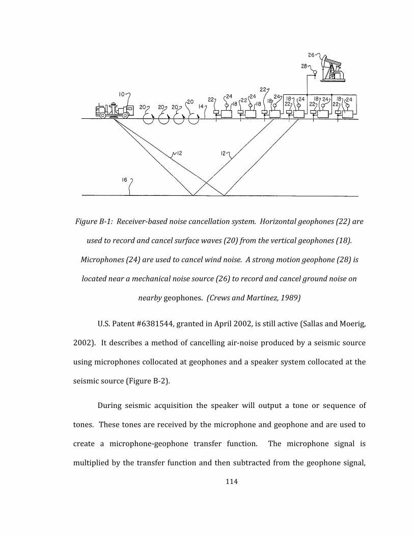
114

Figure B-1: Receiver-based noise cancellation system. Horizontal geophones (22) are

used to record and cancel surface waves (20) from the vertical geophones (18).

Microphones (24) are used to cancel wind noise. A strong motion geophone (28) is

located near a mechanical noise source (26) to record and cancel ground noise on

nearby geophones. (Crews and Martinez, 1989)

U.S. Patent #6381544, granted in April 2002, is still active (Sallas and Moerig,

2002). It describes a method of cancelling air-noise produced by a seismic source

using microphones collocated at geophones and a speaker system collocated at the

seismic source (Figure B-2).

During seismic acquisition the speaker will output a tone or sequence of

tones. These tones are received by the microphone and geophone and are used to

create a microphone-geophone transfer function. The microphone signal is

multiplied by the transfer function and then subtracted from the geophone signal,

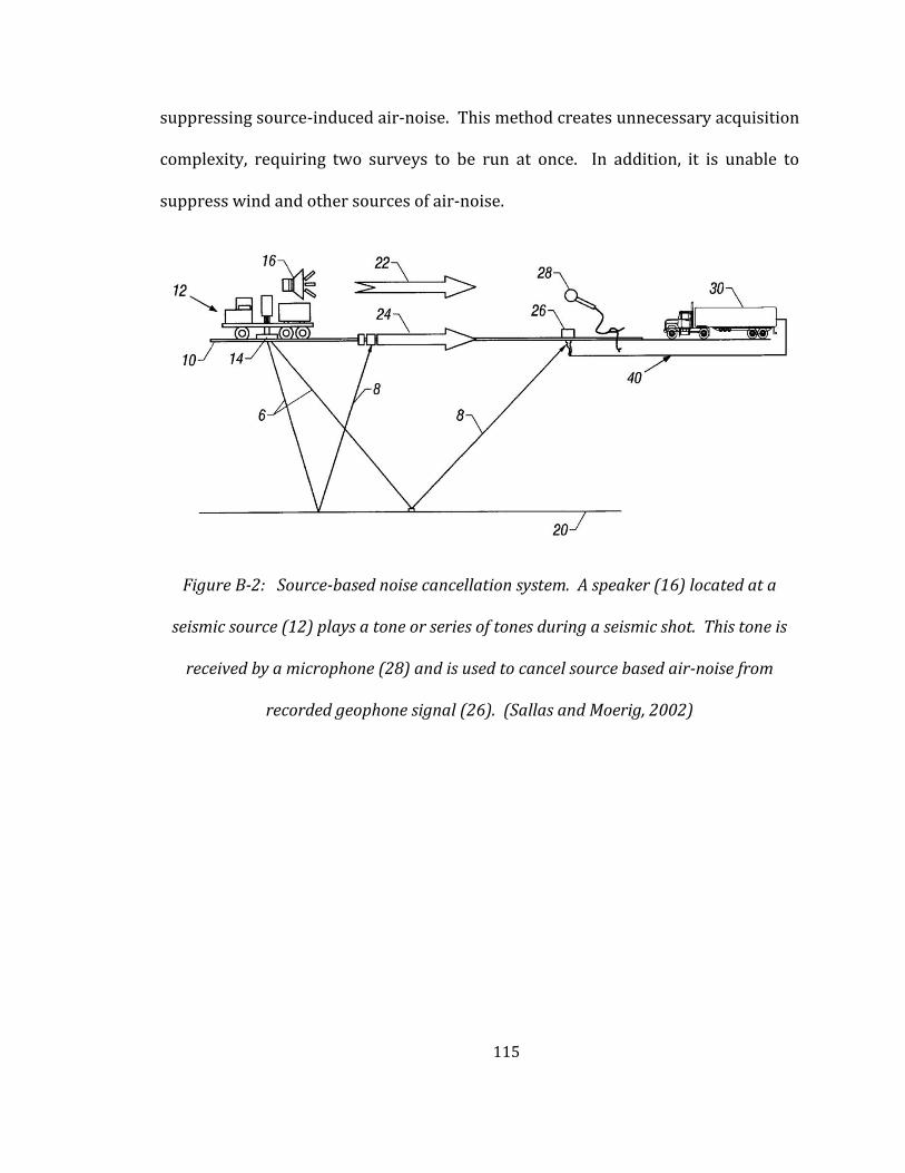
115

suppressing source-induced air-noise. This method creates unnecessary acquisition

complexity, requiring two surveys to be run at once. In addition, it is unable to

suppress wind and other sources of air-noise.

Figure B-2: Source-based noise cancellation system. A speaker (16) located at a

seismic source (12) plays a tone or series of tones during a seismic shot. This tone is

received by a microphone (28) and is used to cancel source based air-noise from

recorded geophone signal (26). (Sallas and Moerig, 2002)

116

REFERENCES

Alcudia, A. D., 2009, Microphone and geophone data analysis for noise

characterization and seismic signal enhancement: M.Sc thesis, University of

Calgary.

Bland, H. C., and E. V. Gallant, 2001, Wind noise abatement for 3-C geophones:

CREWES Research Report, 13.

Crews, G. A., and D. R. Martinez, 1989, Seismic exploration method and apparatus for

cancelling non-uniformly distributed noise: United States Patent 4890264.

Dey, A. K., R. R. Stewart, L. R. Lines, and H. C. Bland, 2000, Noise suppression on

geophone data using microphone measurements: CREWES Research Report,

12.

Google, DigitalGlobe, Houston-Galveston Area Council, Texas General Land Office,

Texas Orthoimagery Program, U.S. Geologic Survey, and USDA Farm Service

Agency, 2012, UH Coastal Center: La Marque, Texas, accessed 06/15/2012,

satellite imagery.

Hansen, T., 2011, SegyMAT: Revision 1.5, website: segymat.sourcefourge.net.

Hedlin, Michael A. H., and Richard Raspet, 2003, Infrasonic wind-noise reduction by

barriers and spatial filters: The Journal of the Acoustical Society of America,

114, 1379.

Hons, M. S., and R. R. Stewart, 2007, MEMS for the masses part 1: comparison to

geophones in theory: CREWES Research Report, 19.

117

Kromer, R. P, 2000, Infrasound sensor models and evaluation: Defense Center

Information Center document.

Press, F., and M. Ewing, 1951, Ground roll coupling to atmospheric compressional

waves: Geophysics, 16, 416.

Sabatier, J. M., H. E. Bass, and L. N. Bolen, 1986a, Acoustically induced seismic waves:

The Journal of the Acoustical Society of America, 80, 646.

Sabatier, J. M., H. E. Bass, and L. N. Bolen, 1986b, The interaction of airborne sound

with the porous ground: the theoretical formulation: The Journal of the

Acoustical Society of America, 79, 1345.

Sallas, J. J., and R. Moerig, 2002, Deterministic cancellation of air-coupled noise

produced by surface seimic sources: United States Patent 6381544.

Shields, D. F., 2005, Low-frequency wind noise correlation in microphone arrays:

The Journal of the Acoustical Society of America, 117, 3489.

Søndergaard, P. L., B. Torrésani, and P. Balazs, 2011, The linear time frequency

analysis toolbox: International Journal of Wavelets, Multiresolution and

Information Processing, 10, website: ltfat.sourceforge.net.

Stewart, R. R., 1998, Air-noise reduction on geophone data using microphone

records: CREWES Research Report, 10.

Withers, M. M., R. C. Aster, C. J. Young, and E. P. Chael, 1996, High-frequency analysis

of seismic background noise as a function of wind speed and shallow depth:

Bulletin of the Seismological Society of America, 86, 1507.

microphone suppression of air-noise … suppression of air-noise on geophones----- a thesis...

Documents