microgravimetric and gravity gradient techniques for

GEOPHYSICS. VOL. 49, NO. 7 (JULY 1984); P. 1084-1096, 23 FIGS.

Microgravimetric and gravity gradient techniques for detection of subsurface cavities

Dwain K. Butler*

-_ __ -- _- __ .._

.ABSTRACT

Microgravimetric and gravity gradient surveying techniques are applicable to the detection and delineation of shallow subsurface cavities and tunnels. Two case histories of the use of these techniques to site investigations in karst regions are presented. In the first case history, the delineation of a shallow (_ 10 m deep), air- filled cavity system by a microgravimetric survey is demonstrated. Also, application of familiar ring and center point techniques produces derivative maps which demonstrate (1) the use of second derivative techniques to produce a “residual” gravity map, and (2) the ability of first derivative techniques to resolve closely spaced or complex subsurface features. In the second case history, a deeper (-30 m deep), water-filled cavity system is adequately detected by a microgravity survey. Results of an interval (tower) vertical gradient survey along a profile line are presented in the second case history; this vertical gradient survey successfully detected shallow (< 6 m) anomalous features such as limestone pinnacles and clay pockets, but the data are too “noisy” to permit detection of the vertical gradient anomaly caused by the cavity system. Interval horizontal gradients were determined along the same profile line at the second site, and a vertical gradient profile is determined from the horizontal gradient profile by a Hilbert transform technique. The measured horizontal gradient profile and the computed vertical gradient profile compare quite well with corresponding profiles calculated for a two-dimensional model of the cavity system.

~~-- __ -- -----

BACKGROUND

Detection and delineation of subsurface cavities is one of the most frequently cited applications of microgravimetry. Cavities may be natural, such as solution cavities in limestones, dolo- mites, and evaporites; or man-made, such as tunnels or mines; and may be air-filled, water-filled, or filled with some secondary geologic material. A potential field method, such as gravimetry or magnetic methods (in the latter instance only if the cavities

represent a magnetic polarization contrast), is well suited for the detection and delineation of cavities; whereas cavities present a very difficult objective for detection by other geophysical methods (Franklin et al., 1980; Butler, 1977). Solution cavities are just part of the geologic complexity to be expected in karst regions, and microgravimetry is an invaluable complement to other geophysical, geologic, and direct methods for site investigations in such areas.

Butler (1980) reviewed case histories of subsurface cavity detection investigations by Arzi (1975) Neumann (1977), and Fajklewicz (1976). The work by Arzi and Neumann involved microgravimetric surveys which delineated karstic cavities and abandoned mines, respectively; while the work by Fajklewicz involved the use of a tower structure to measure interval vertical gradients for the detection of shallow (< 15 m) abandoned mines. Although Fajklewicz reported an impressive anomaly verification record, his paper generated considerable dis- cussion. Much of the negative reaction to the work of Fajkle- wicz came from accuracy and precision claims for his data which seemed to be inconsistent with the accepted accuracy (f 20 uGa1) of the Sharpe gravimeter which he used.

A research program was initiated in 1976 at the U. S. Army Engineer Waterways Experiment Station to investigate geophysical methodologies for detection and delineation of subsurface cavities. The work was conducted in three phases:

(1) assessment of geophysical methods for cavity detection at a man-made cavity test ‘site (Butler and Murphy, 1980);

(2) assessment of geophysical methods for cavity detection at a shallow (5 10 m), air-filled, natural cavity test site, Medford Cave, Marion County, Florida (Butler, 1980, 1983; Ballard, 1983; Curro, 1983; Cooper, 1983); and

(3) assessment of the most promising geophysical methods, identified in phase 2, at a deeper (- 30 m), water- filled cavity test site, Manatee Springs, Levy County, Florida (Butler et al., 1983).

One of the conclusions of this work is that, for investigations requiring detection and delineation of shallow cavities ( 6 4 to 6 effective cavity diameters in depth), microgravimetry is the most promising surface method in most cases.

Manuscript received by the Editor January 11, 1983; revised manuscript received January 16, 1984. *US. Army Engineer Waterways Experiment Station, P.O. Box 631, Vicksburg, MS 39180. This paper was prepared by an agency of the U.S. government.

1084

1085 Gravity Detection, Subsurface Cavities

FIG. 1. Cavity map, survey grid, and borehole locations at the Medford Cave site.

In this paper, results of microgravimetric surveys at the Medford Cave and Manatee Springs test sites are presented. Details of site characteristics, topographic survey procedures, microgravimetric field procedures, data collection procedures, etc., are presented in the references given under the phase 2 and 3 descriptions of the research program. The presentation here will concentrate on the aspects of work at the two sites related to gravity-gradient measurements and/or determinations. Med- ford Cave is a complex, three-dimensional (3-D) system; thus gravity gradient methods were restricted to analytical determination by the familiar ring and center point techniques, albeit on a very dense grid of stations. In the vicinity of the microgravimetric survey, the Manatee Springs cave system can be considered an approximately two-dimensional (2-D) feature. Thus at Manatee Springs, interval vertical and horizontal gradients were determined along a profile line approximately perpendicular to the axis of the main cavity system, and procedures for

calculating vertical gradient profiles from horizontal gradient profiles by application of a discrete Hilbert transform, valid for 2-D cases, are investigated.

MEDFORD CAVE SITE INVESTIGATIONS

Scope of microgravimetric survey

The microgravity survey at Medford Cave site consisted of 420 stations over a 260 by 260 ft’ (approximately 80 by 80 m) area. A basic grid dimension of 20 ft (6.1 m) was used, with a IO-ft (3-m) grid used in the central portion of the area over the known cavity system. A LaCoste and Romberg model D-4

‘Grid and profile dimensions for the two test sites are in feet. Gradi- ents are converted to mGal/m.

1088 Butler

FIG. 2. Cross-section cavity maps of the Medford Cave site.

gravity meter’ was used for the survey. Figures 1 and 2 present plan and cross-section views of the known cavity system, and Figure 3 is the site topographic map.

Grid point (0, 0) was selected as the base station and was reoccupied at least once per hour. The gravity meter was oper- ated at night in a tidal recording mode to produce a tidal record for comparison with the field base station “drift” curve. Figure 4 shows the comparison between the measured tidal curve and the base station drift data. The long-term, cumulative drift (nontidal) of the gravity meter appears to be about 2 uGal/hr, although there are nontidal meter drifts larger than this that are not cumulative.

selective drilling of small negative anomalies in areas away from the known cavity system intercepted air- or clay-filled cavities or clay pockets in the top of the limestone. Eleven boreholes were located in positive anomaly areas, and only three of these boreholes intercepted cavities (Z2 ft in vertical dimension). Figure 7, for example, compares a gravity profile

Residual gravity anomaly maps

The data were processed and corrected using the procedures outlined in Butler (1980) and Butler et al. (1983). A density of 1.9 g/cm” was used for the Bouguer and terrain corrections based on density measurements on near-surface soil and rock samples from the site. A total of 61 stations near the three sinkholes required terrain corrections > 10 uGa1. Figures 5 and 6 are resulting residual gravity anomaly maps for the basic 20 ft grid data set and for all the data (including 10 ft grid data), respectively, after removal of a planar regional field determined by inspection. Correlation of gravity anomalies with features of the known cavity system as shown in Figure 3 is excellent, and

‘The model-D gravimeter has a sensitivity to gravity change or variation of approximately 1 PGal and an accuracy of k4 pGal in the determination of a single relative gravity value using exacting field procedures. FIG. 3. Topographic map of the Medford Cave site.

Gravity Detectfon, Subaurffme Cavltles

FIG. 4. Drift curve and measured earth tide curve for the Medford Cave site microgravimetric survey.

along a north-south line (the 8OW line) with a geologic cross- section along the line determined by closely spaced exploratory drilling. The correlation of gravity lows and highs with clay pockets and limestone pinnacles, respectively, in the 110 to 260 ft profile range is quite good.

Gravity gradient maps

Two types of gravity-gradient maps were generated from the Medford Cave site microgravity survey data. The familiar ring

and center point (spatial filtering) techniques were utilized to compute first (vertical gradient) and second derivative maps from the gravity data. These techniques were used for this site for two reasons: (1) to investigate the application of the techniques to small-scale surveys for improved resolution and the de’termmatron of residual gravity maps; and (2) because the known cavity system is clearly threedimensional. Since the techniques are familiar and standard, details about their formu- lation and use will not be given.

The second derivative map in Figure 8 was produced using

FIG. 5. Residual gravity anomaly map, 20 ft data spacing, FIG. 6. Residual gravity anomaly map, 10 ft data spacing, Medford Cave site microgravimetric survey. Medford Cave site microgravimetric survey.

1088 Butler

FIG. 7. Comparison of the 80W north-south residual gravity profile with the known geologic cross-section.

an equation due to Elkins (1951). This technique is sometimes referred to as the Elkins residual method, since it is designed to produce a map closely resembling a residual gravity map. Use of a ring at rr = a = 20 ft (6.1 m) introduces a second derivative filtering with coefficients chosen to smooth high spatial fre-

FIG. 8. Second derivative map (Elkins’ residual) produced from the Bouguer anomaly data from the Medford Cave site survey.

FIG. 9. First derivative map produced from the Bouguer anom-

Contour interval = 1 (arbitrary units). aly data from the Medford Cave site survey. Contour interval = 1 (arbitrary units).

quencies; while a second ring at r4 = & a = 44.7 ft (13.6 m) is

used to approximate a local regional field for the center point. The contour values in Figure 8 should be considered in a relative sense with arbitrary units.3 Comparing the second derivative map in Figure 8 with the residual gravity map in Figure 5, the similarity is evident. All of the primary features of the residual gravity map can be found in the second derivative map. The second derivative technique is a more objective procedure than the inspection or graphical techniques, and it can be advantageously applied to microgravity survey results when it is difficult to recognize the proper scale regional field.

Figure 9, the vertical gradient or first derivative map, was produced using an equation due to Baranov (1975). The equation does not have coefficients chosen to produce smoothing as in the second derivative equation. Thus, in principle, the first derivative map should have greater resolution than the second derivative and residual gravity map. The contour values in Figure 9 should be considered in a relative sense with arbitrary units.4 All of the anomaly features identified on the residual gravity map can be seen on the first derivative map; however, the spatial extent of given anomalies is generally less on the first derivative map than on the residual gravity map. Also, some anomalies observed as single features on the residual gravity map seem to be resolved into two or more features on the first derivative map, such as the negative anomaly between 80N and 180N in Figure 5 along the eastern boundary of the survey area.

3As emphasized by one reviewer, this procedure produces only a very poor approximation to the true second vertical derivative due to the strong smoothing involved in the filter operator. Thus the second derivative map should be used only for the location of anomalies in plan and not for any type of quantitative interpretation. ‘Strictly speaking,, first derivative units, the Eotvos (E), can be obtained by multiplymg contour values by 18.31365.

Gravity Detection, Subsurface Cavities 1089

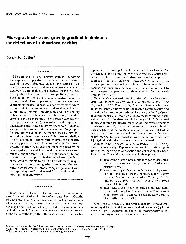
FIG. 10. Comparison of residual gravity (g,), first derivative (g:), and second derivative (9:) profiles along the 0 north-south line.

In order to compare and evaluate the features of the derivative and residual gravity maps, two north-south profile lines were selected for study. The 0 north-south profile line was chosen due to the interesting negative anomaly centered at (110, 0) and because it is representative of areas at the site about which nothing was known prior to verification drilling. The residual gravity, first derivative, and second derivative profiles along the C north-south line are shown in Figure 10. All three profiles show.the negative anomaly feature between profile locations 80 and 180. The gravity profile suggests that there might be two closely spaced subsurface features causing the anomaly (or at least a significant change in shape, size, or density contrast of the feature). The second derivative profile shows essentially the same information as the residual gravity profile. The first derivative profile, however, clearly resolves the anomaly into two negative anomalies centered at the 1 lo- and 160-ft profile locations. Verification drilling was not extensive

FIG. 11. Comparison of residual gravity (g,), first derivative (gi), and second derivative (gi) profiles along the 8OW north-south line.

enough to confirm in detail the predictions of multiple subsurface features causing the negative anomaly, but two boreholes placed at (110, 0) and (117, - 5) confirmed the presence of a significant cavity feature at this location which varied in dimension and depth laterally.

The 80W north-south profile line was discussed previously in connection with the residual gravity profile; the gravity profile is compared with the gravity-gradient profiles for this line in Figure 11. Qualitatively, all three profiles in Figure 11 are similar. The smoothing inherent in the second derivative procedure is evident in the subdued nature of the highs and lows corresponding to the limestone pinnacles and clay pockets. The first derivative profile in this case, however, is nearly identical to residual gravity profile in delineating the top of limestone topography and detecting the known cavity (see Figure 7).

MANATEE SPRINGS SITE INVESTIGATIONS

Scope of microgravimetric

and gravity-gradient surveys

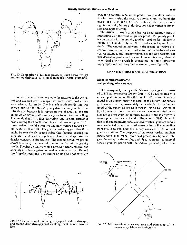
The microgravity survey at the Manatee Springs site consisted of 186 stations over a 100 by 400 ft (- 30 by 122 m) area with a basic grid interval of 20 ft (6.1 m). A LaCoste and Romberg model D-25 gravity meter was used for the survey. The survey grid was oriented approximately perpendicular to the known trend of the cavity system as shown in Figure 12. Grid point (0, 200) was used as a base station and was reoccupied on an average of once every 30 minutes. Details of the microgravity survey procedure can be found in Butler et al. (1983). In addi- tion to the microgravity survey, a tower vertical gradient survey was conducted along the southwest-northeast line extending from (40, 0) to (40, 400); this survey consisted of 21 vertical gradient stations. The purposes of the tower vertical gradient survey were (1) to refine tower field procedures, (2) to investigate the utility of the results, and (3) to compare the interval vertical gradient profile with the vertical gradient profile com-

FIG. 12. Microgravimetric survey area and plan map of the main cavity, Manatee Springs site.

FIG. 13. Bouguer gravity anomaly map, Manatee Springs site.

A

. . . . * ,oo J . . . .

. . / . i100.400)

I ,L 20p0.1

puted as the discrete Hilbert transform of an interval horizontal gradient profile.

Residual gravity anomaly maps

Part of the research effort at the Manatee Springs site was dedicated to a comparison of the results of selecting a local regional field by inspection and by a more objective procedure such as polynomial surface fitting. Figure 13 is the Bouguer anomaly map (1.8 g/cm3 used for Bouguer and terrain corrections) for the survey area; the maximum gravity difference between any two points in the grid is only - 80 uGa1. A careful inspection of gravity values and means along the grid lines led

to the selection of a planar regional field dipping from southeast (SE) to northwest (NW) with a gradient of 0.22 uGal/ft (0.72 @al/m). Subtracting this “inspection regional” gives the residual map shown in Figure 14; the plan view of the cavity system, determined by cave divers during the course of the field work, is also shown (the plan map shown in Figure 12 is the detail known prior to the field work).

The broad negative anomaly over the known cavity system in Figure 14 is consistent in magnitude and width with the known size and depth of the cavity system. However, there are complexities or smaller anomalous features in the residual map which cannot be attributed to the main cavity; some of these smaller anomalies may be due to smaller and shallower solution features or other density anomalies. The basic concept of

FIG. 14. Residual gravity anomaly map, Manatee Springs site.


. . . . . .

2. 0

/.’

/

P’

/ &+‘

/ / . s?

(O*O’SECOND ORDER

. . . . . x(

L i \L

FIG. 15. First- through fourth-order polynomial surface fits to the Bouguer gravity data (see Figure 13); contour interval = 10 PGal.

the polynomial surface-fitting technique for determining regional fields is that successively higher order surface fits to the Bouguer anomaly data account for the gravity effects of successively smaller and shallower subsurface features (Coons et al., 1967; Nettletoli, 1971). Figure 15 contains contoured polynomial surface fits.to the Bouguer data through fourth order. It is noteworthy that, although the first-order (planar) surface dip through the grid is on a different azimuth than the plane determined by inspection, the southeast-northwest gradient is the same, i.e., -0.22 uGal/ft. The residual anomaly map, obtained by subtracting the first-order surface fit, is shown in Figure 16. Further details of the surface-fitting procedure and

features of higher order residual maps are given in Butler et al. (1983). The map of second-order residual, for example, displays a small closed negative anomaly feature at location (100, 220) which was verified when a wheel of a drill rig collapsed a soil bridge revealing a vertical solution pipe about 80 ft deep.

Vertical gradient survey results

Using a specially adapted tripod, the five measurement elevations illustrated in Figure 17 were utilized during the vertical gradient survey along the (40, 0) to (40, 400) survey line. Only

FIG. 16. First-order residual gravity anomaly map, Manatee Springs site.

Butler

--h,

FIG. 17. Illustration of the tower or tripod measurement concept for vertical gradient determination; for the Manatee Springs survey, nominal values for he, h,, h, , h, , and h, are 0, 0.60,0.78, 1.38, and 1.63 m, respectively.

0.27

five gravity values at the upper elevation h, were obtained along the profile line. The measurement sequence at each profile location required 1.5 to 25 minutes; thus the ground station h, was reoccupied at the end of each sequence and the data were drift-corrected in the usual manner.

Considering elevations h,, h,, h, , and h, , six interval gradients can be determined as well as differential gradients at any point within the interval h, to h, using a parabolic fitting procedure. Results of three of the determinations of vertical gradients along the (40, 0) to (40, 400) survey line are shown in Figure 18; Agb,/Az,,, and AgbJAze3, where AgbI = go - gr, A”,,, = h, - h,, etc., and (Cg/iiz),, which is the differential gradient at h, determined from a parabolic fit to the data at h,, h,, and h,. The five values of Agb,/Az,,, are also shown. All three profiles exhibit considerable variation, with several gradient anomalies as large as 10 percent of the normal vertical gradient. The Agb3/Azo3 p refile is smoother than the other profiles, since it is less affected by very shallow density anomalies (Butler, 1984). All three profiles behave qualitatively the same except at profile positions 0,40 to 60,200, and 360 where the Agb3/Azo3 profile behavior is clearly at variance with the other two profiles. In many locations the three values are nearly identical; and at the 100 and 300 ft profile positions all four values are nearly equal and also nearly equal to the normal gravity gradient, which implies a linear variation of gravity with elevation at these locations. There are, however, no obvi- ous indications of an anomaly which could be caused by the main subsurface cavity system.

Horizontal gradient determinations

Using the gravity data along the selected profile line, horizontal gradient profiles can be determined using various values

0 50 100 150 200 250 300 350 400

X, FT

(DISTANCE ALONG SURVEY GRID PROFILE LINE FROM 40.0 TO 40.4001

FIG. 18. Profile of interval vertical gradient determinations, Manatee Springs site.

0.02

0.01

E

2

2

0 2 >

B

z

-0.01

-0.02


EXTENT OF CAVITY

(FIG. 14)

50 100 150 200 250 3”U 3!xl 400

X. FT

FIG. 19. Profiles of interval horizontal gradient determinations, Manatee Springs site.

of AX. Horizontal gradient profiles for Ax equal to 20, 40, and 80 ft (6.1, 12.2, and 24.4 m) are shown in Figure 19, where the residual gravity values from Figure 15 (planar least-squares regional) were used. The profiles in Figure 19 clearly become smoother with increasing Ax, and all three profiles show “average behavior” consistent with the known cavity system with center at profile position 200 ft. The Ax = 20-ft profile, however, is so erratic that the “cavity gradient signature” is effectiveiy masked. The gradient “signature” of rhe cavity is enhanced by Ax values which are larger than the effective depths of the shallow anomalous features causing the erratic behavior of the AX = 20-ft profile (Butler, 1984). Accordingly, the AX = SO-ft profile data will be used for the considerations which follow.

Comparison of results with 2-D model calculations

The cavity system was modeled as a 2-D prism with rec- tangular cross-section as shown in Figure 20 (based on cavity details known prior to the field work), and interval horizontal and vertical gravity gradients were computed. In Figure 21, the computed horizontal gradient profile is compared with the measured horizontal gradient profile for Ax = 80 ft. The average behavior of the measured profile approximates the calculated profile quite well in amplitude and spatial wavelength, with the amplitude of the measured profile slightly larger on the right-hand side. The vertical gravity gradient g_(x, z) on the surface z = 0, due to a 2-D subsurface structure, is related to the horizontal gravity gradient g_(x, z) on the surface by a Hilbert transform (Sneddon, 1972, Bracewell, 1965),

where x is the profile point at which CJ,, z is to be determined. An algorithm for computing the vertical gradient of a discrete horizontal gradient profile data set is presented in Butler et al. (1982) using a procedure suggested by Shuey (1972). A vertical

FIG. 20. Two-dimensional model of the main cavity at the Manatee Springs site and the calculated gravity anomaly.

Butler

0.002 -

- MEASURED HORIZONTAL

$ 0.001 - GRADIENT, Ag,/AX. AX=80 FT m

: ---- CALCULATED HORIZONTAL

GRADIENT. 2-D MODEL, K

6

AX=80 FT

E

2 0 u

<

z N

6 1 -0.001 -

EXTENT OFYODEL CAVITY

~,EXT.NT OF MAPPED CAVITY

-0 002 1 I I I I I I I

0 100 200 300 400

X, FT

FIG. 21. Comparison of measured and calculated horizontal gravity gradient profiles, Manatee Springs site.

gradient profile, computed by the Hilbert transform procedure Using the profiles in Figures 21 and 22, gradient space plots from the measured horizontal gradient profile for Ax = 80 ft, is are shown in Figure 23 for the 2-D model and for data from the compared to the vertical gradient profile computed from the field measurements. In the gradient space plot, each point 2-D model in Figure 22. Again, the agreement between the two represents the interval horizontal and vertical gradients of a profiles in Figure 22 is good with respect to amplitude and given profile position x, and the arrows indicate traversing the spatial wavelength. However, the Hilbert transform profile has profile line in the positive x-direction. The somewhat subtle maximum amplitude at position 240 ft rather than 200 ft and differences noted in the profile data plots are more apparent in has a prominent positive peak at 320 ft. Clearly, no meaningful the gradient space plot; to profile position 200 ft (lower half of comparison can be made between the profiles in Figure 22 and plots in Figure 23), the agreement between the two plots is the measured interval vertical gradient profiles in Figure 18. good, but from profile positions 200 to 400 ft (upper half of The amplitude of the vertical gradient anomaly due to the plots in Figure 23), the two plots differ significantly in mag- cavity is much too small to be detected with a short tower in the nitude. The results in Figure 23 suggest that the simple 2-D presence of the “noise” evident in Figure 18. model which was selected does not approximate the cavity

0 002

1 - HD1~g,/~X). AX = 80 FT

-_- ~g’,,AZ. FROM 2-D MODEL E 0001 -

L m

E

i \ --_ 0

2 0 0

2 r E >

-0.001 -

EXTENT OF MODEL CAVITY

EXTENT OF MAPPED CAVITY

-0 002 I

0 100 200 300 400

X. FT

FIG. 22. Comparison of a vertical gravity gradient profile computed as the discrete Hilbert transform HD of the measured horizontal gradient profile (Figure 21) with a vertical gradient profile computed for the 2-D model (Figure 20).


mGal/m

0 002 T - 2-D MODEL

- * - FROM FIELD DATA

1 Ag’JAz -0.002 0.002 mGal/m

-0.002 A-

FIG. 23. Comparison of gradient space plots from field data and from 2-D model calculations, Manatee Springs site.

system very well. Indeed, both reports of the cave diving team and a very limited verification drilling effort confirm that the cavity system is extremely complex. The cavity varies errati- cally in cross-sectional shape and size; a vaulted ceiling is common and numerous smaller branching cavities are present. Also, drilling and detailed mapping indicates more extensive solutioning to the northeast of the (0, 200) to (100, 200) line than southwest of it, which is consistent with both the residual gravity map and the gravity-gradient results.

Verification of drilling results

Only a limited number of verification borings were possible, and the borings were located to investigate various gravity anomalies as well as anomalies indicated by other geophysical surveys and not specifically to investigate anomalies along the gravity-gradient profile line. Likewise, borings placed to ac- c~ommodate crosshoie geophysicai surveys of various types were placed to the northeast of the gradient profile line for the most part. Two of the borings, however, allow direct confir- mation of vertical gradient anomalies shown in Figure 18. The borings indicate that, typically, limestone is encountered at depths of 13 to 17 ft, although limestone pinnacles are within 5 ft of the surface in places and clay-filled pockets in the top of the limestone extend to depths of 27 ft in places. A boring near gradient profile position 120 ft encountered a clay pocket which extended to the 27-ft depth (limestone is typically encountered at the 17-ft depth in this area); the vertical gradient profiles show a prominent negative anomaly at this location. Another boring near gradient profile position 280 ft encountered a clay pocket extending to the 16-ft depth (limestone is typically encountered at the 13-ft depth in this area); the vertical gradient profiles show a~negativeanomaly at~tbis location.

The microgravity survey of the Manatee Springs site successfully detected the main water-filled cavity system. Results of drilling at the Manatee Springs site confirm that the large magnitude, short spatial wavelength anomalies which appear in the measured interval vertical gradient profiles are due primarily to relatively shallow ( < 20 ft) density anomalies such as clay pockets and limestone pinnacles. The lower amplitude, longer spatial wavelength anomalies which appear in the measured horizontal gradient and Hilbert transform vertical gradient profiles are due to the deeper (> 80 ft) main cavity system. The large amplitudes of the vertical gradients due to shallow features at the Manatee Springs site completely mask any possible expression in the measured interval vertical gradient profile of the low amplitude anomaly due to the deeper cavity system. A much taller tower (>20 ft in height) with lower measurement stations several feet above the ground would be required to have any chance of detecting the small vertical gradient anomaly caused by the cavity system.

The considerable flexibility in the selection of horizontal intervals from the Manatee Springs survey for determining interval horizontal gradient profiles allowed a profile to be selected which (1) appears to be free from significant pertur- bation due to shallow anomaious features, (2) is consistent with the known location and general features of the main cavity system, and (3) compares quite well with an interval horizontal gradient profile computed from an approximate 2-D model of the cavity. Using the horizontal gradient profile with an interval selected to attenuate gradient anomalies caused by shallow density variation, a vertical gradient profile was computed by a discrete Hilbert transform which compares satisfactorily with the vertical gradient profile of the approximate 2-D model. While these results are demonstrated for a specific case study, the procedures are general and can be applied to any feature which is approximately two-dimensional. The gradient profiles produced by this procedure can then be utilized in combined gradient interpretive procedures such as discussed by Nabi- ghian (1972), Stanley and Green (1976), Hammer and Anzol- eaga (I 975), and &tier et al. (198j.

The boring near gradient profile position 280 ft encountered The usefulness of interval vertical gradient surveys, using a significant clay-filled cavity in the 90- to 105-ft depth range; towers of manageable height (l-4 m), is primarily limited to this is the same depth range as the known water-filled cavity to exploration for shallow targets (< 10-15 m), such as solution

the southwest. The discovery of this clay-filled cavity feature suggests that solution features extend considerably northeast of the known cavity system under the gradient profile line, which is completely consistent with the gradient profile data in Fig- ures 21-23.

CONCLUSIONS

The microgravity survey at the Medford Cave site demon- strates the capability of microgravimetry to detect and delin- eate shallow, complex cavity systems. Familiar spatial filtering techniques were applied to the dense grid of gravity stations to produce first and second vertical derivative maps. Suitable selection of ring radii and coefficients in a second derivative equation successfully produced a map which compares quite well with residual gravity maps produced by the usual regional- residual separation procedure. Examination of a selected profile line from the first derivative (vertical gradient) map demon- strates the greater resolving power of the first derivative profile compared to the gravity profile.

1096 Butler

cavities and abandoned mines (Fajklewicz, 1976; Butler, 1980). There is no flexibility to select large vertical intervals in order to attenuate large gradient anomalies caused by shallow density variations. Also, since terrain variations produce large vertical gradient effects on short tripod measurements (Fajkle- wicz, 1976; Ager and Liard, 1982), interval vertical gradient surveys will be most successful in areas with flat terrain. Thus, interval vertical gradient surveys are not useful, in general, for combined gradient interpretive procedures.

REFERENCES

Ager, C. A., and Liard, J. O., 1982, Vertical gravity gradient surveys: Field results and interpretations in British Columbia. Canada: Geo- physics, v. 47, p. 919-925.

Arzi, A. A., 1975, Microgravimetry for engineering applications: Geo- phys. Prosp., v. 23, p. 408425.

Ballard, R. F., 1983, Cavity detection and delineation research, Report 5, Electromagnetic (radar) techniques applied to cavity detection: Tech. Rept. CL-83-1, U. S. Army Engineer Waterways Experiment Station, CE, Vicksburg, MS.

Baranov, W., 1975. Potential fields and their transformations in au- plied geophysics: Geoexpl. Monographs, Series 1, no. 6, Berlin, Geopublication Associates.

Bracewell, R. N., 1965, The Fourier transform and its applications: New York, McGraw-Hill Book Co. Inc., 352 p.

Butler, D. K., Ed., 1977, Proc. of the symposium on detection of subsurface cavities: U. S. Army Engineer Waterways Experiment Station, CE, Vicksburg, MS.

~ 1980, Microgravimetric techniques for geotechnical applications: Miscellaneous Paper CL-80-13, U. S. Army Engineer Waterways Experiment Station, CE, Vicksburg, MS.

~ 1983, Cavity detection research, Report 1, Microgravimetric and magnetic surveys, Medford Cave Site, Florida: Tech. Rep. GL- 83-1, U. S. Army Engineer Waterways Experiment Station, CE, Vicksburg, MS

__ 1984, Gravity gradient determination concepts: Geophysics, v. 49, p. 8288832.

Butler, D. K., and Murphy, W. L., 1980, Evaluation of geophysical methods for cavity detection at the WES cavity test facility: Tech. Rep. CL-80-4, U. S. Army Engineer Waterways Experiment Station, CE, Vicksburg, MS.

Butler, D. K., Gangi, A. F., Wahl, R. E., Yule, D. E., and Barnes, D. E., 1982, Analytical and data processing techniques for interpretation of geophysical survey data with special application to cavity detection: Misc. paper CL-82-16, U. S. Army Engineer Waterways Experiment Station, CE, Vicksburg, MS.

Elkins, T. A., 1951, The second derivative method of gravity interpretation: Geophysics, v. 16, p. 29950.

Butler, D. K., Whitten, C. B., and Smith, F. L., 1983, Cavity detection research, Report 4, Microgravimetric survey, Manatee Springs Site, Florida: Tech. Rep. CL-83-1, U. S. Army Engineer Waterways Ex- periment Station, CE, Vicksburg, MS.

Cooper, S. S., 1983, Cavity detection and delineation research, Report 3, Acoustic resonance and self-potential applications_Medford Cave and Manatee Springs Sites, Florida: Tech. Rep. CL-83-1, U. S. Army Engineer Waterways Experiment Station, CE, Vicksburg, MS.

Coons, R. L., Woollard, G. P., and Hershey, G., 1967, Structural significance and analysis of Mid-Continent gravity high: Bull., Am. Assoc. Petr. Geol., v. 51, p. 2381-2409.

Curro, J. R., 1983, Cavity detection and delineation research, Report 2, Seismic Methodology-Medford Cave Site, Florida: Tech. Rep. GL- 83-1, U. S. Army Engineer Waterways Experiment Station, CE, Vicksburg, MS.

Fajklewicz, Z. J., 1976, Gravity vertical gradient measurements for the detection of small geologic and anthropomorphic forms: Geophys- ics, v. 41, p. 10161030.

Franklin, A. G., Patrick, D. M., Butler, D. K.? Strohm, W. E., and Hvnes-Griffin. M. E.. 1980. Foundation constderations in siting of nuclear facilities in karst terrains and other areas susceptibl; to ground collapse: NUREGCR-2062, U. S. Nucl. Reg. Commission, Washington, D. C.

Hammer, S.: and Anzoleaga, R., 1975, Exploring for stratigraphic traps with gravtty gradients: Geophysics, v. 40, p. 256268.

Nabighian, M. N.. 1972. The analytic sianal of two-dimensional magnetic bodies with polygonal cross-secti&-Its properties and use for automated anomaly interpretation: Geophysics, v. 37, p. 507-517.

Neumann, R., 1977, Microgravity method applied to the detection of cavities: Symposium on Detection of Subsurface Cavities, D. K. Butler, Ed: U. S. Army Engineer Waterways Experiment Station, CE, Vicksburg, MS.

Nettleton, L. L., 1971, Elementary gravity and magnetics for geologists and seismologists: Monograph No. 1, Tulsa, Sot. of Expl. Geophys.

Shuey, R. T., 1972, Applications of Hilbert transforms to magnetic profiles: Geophysics, v. 37, p. 1043-1045.

Sneddon, I. N., 1972, The use of integral transforms: New York, McGraw-Hill Book Co. Inc., 539 p.

Stanley, J. M., and Green, R., 1976, Gravity gradients and the interpretation of the truncated plate: Geophysics, v. 41, p. 137&1376.

microgravimetric and gravity gradient techniques for

Documents