microéconomie de la finance -...
TRANSCRIPT
Chapitre 47e édition
La théorie Moyenne-Variance du choix de portefeuille
2
Microéconomie de la finance –Christophe BOUCHER – 2014/2015
Part 4. Mean-Variance Portfolio Theory
3
4.1 Measuring Risk and Return
4.2 Asset Allocation with 2 Risky Assets
4.3 Introducing a Risk Free Asset and the Tobin’s Separation Theorem
4.4 Asset Allocation with N risky Assets
4.5 Portfolio Diversification
Microéconomie de la finance –Christophe BOUCHER – 2014/2015
Preamble:
Mean/Variance Analysis Assumptions
4
Microéconomie de la finance –Christophe BOUCHER – 2014/2015
Mean-variance is simpler
5
• Early researchers in finance, such as Markowitz and Sharpe, used just the mean and the variance of the return rate of an asset to describe it.
• Characterizing the prospects of a gamble with its mean and variance is often easier than using an NM utility function, so it is popular.
• But is it compatible with VNM theory?
• The answer is yes … approximately … under some conditions.
Microéconomie de la finance –Christophe BOUCHER – 2014/2015
Mean-variance assumptions
6
• Investors maximise expected utility of end-of-perio d wealth
• Can be shown that above implies maximise a function of expected portfolio returns and portfolio variance p roviding
- Either utility is quadratic, or
- Portfolio returns are normally distributed (and utility is concave),
- Consider only small risks (then approximately true)
Microéconomie de la finance –Christophe BOUCHER – 2014/2015
Mean-variance: quadratic utility
7
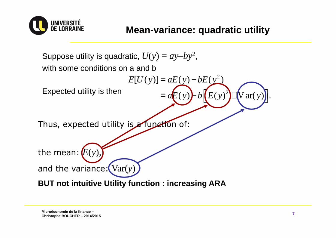
Suppose utility is quadratic, U(y) = ay–by2,
with some conditions on a and b
Expected utility is then
2
2
[ ( )] ( ) ( )
( ) ( ) V ar( ) .
E U y aE y bE y
aE y b E y y
= −
= − +
Thus, expected utility is a function of:
the mean: E(y),
and the variance: Var(y)
BUT not intuitive Utility function : increasing ARA
Microéconomie de la finance –Christophe BOUCHER – 2014/2015
Mean-variance: joint normals
8
• Suppose all lotteries in the domain have normally distributed prized. (They need not be independent of each other).
• Any combination of such lotteries will also be normally distributed.
• The normal distribution is completely described by its first two moments.
• Therefore, the distribution of any combination of lotteries is also completely described by just the mean and the variance.
• As a result, expected utility can be expressed as a function of just these two numbers as well.
Microéconomie de la finance –Christophe BOUCHER – 2014/2015
Mean-variance: small risks
9
• The most relevant justification for mean-variance is probably the case of small risks.
• If we consider only small risks, we may use a second order Taylor approximation of the NM utility function.
• A second order Taylor approximation of a concave function is a quadratic function with a negative coefficient on the quadratic term.
• In other words, any risk-averse NM utility function can locally be approximated with a quadratic function.
• But the expectation of a quadratic utility function can be evaluated with the mean and variance. Thus, to evaluate small risks, mean and variance are enough.
Microéconomie de la finance –Christophe BOUCHER – 2014/2015
Mean-variance: small risks
10
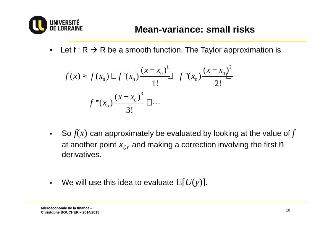
• Let f : R R be a smooth function. The Taylor approximation is
• So f(x) can approximately be evaluated by looking at the value of fat another point x0, and making a correction involving the first nderivatives.
• We will use this idea to evaluate E[U(y)].
1 2
0 00 0 0
3
00
( ) ( )( ) ( ) '( ) ''( )
1! 2!
( )'''( )
3!
x x x xf x f x f x f x
x xf x
− −≈ + + +
−+⋯
Microéconomie de la finance –Christophe BOUCHER – 2014/2015
Mean-variance: small risks
11
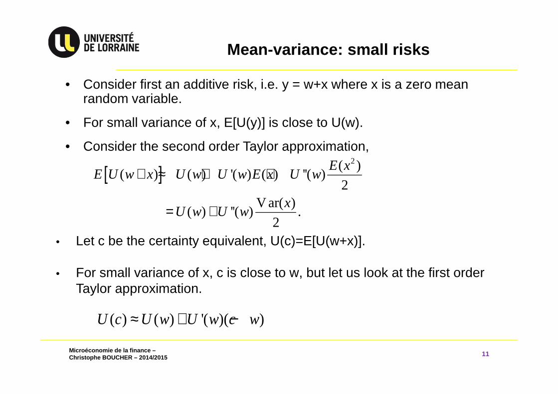
• Consider first an additive risk, i.e. y = w+x where x is a zero mean random variable.
• For small variance of x, E[U(y)] is close to U(w).
• Consider the second order Taylor approximation,
• Let c be the certainty equivalent, U(c)=E[U(w+x)].
• For small variance of x, c is close to w, but let us look at the first order Taylor approximation.
[ ]2( )
( ) ( ) '( ) ( ) ''( )2
V ar( )( ) ''( ) .
2
E xE U w x U w U w E x U w
xU w U w
+ ≈ + +
= +
( ) ( ) '( )( )U c U w U w c w≈ + −
Microéconomie de la finance –Christophe BOUCHER – 2014/2015
Mean-variance: small risks
12
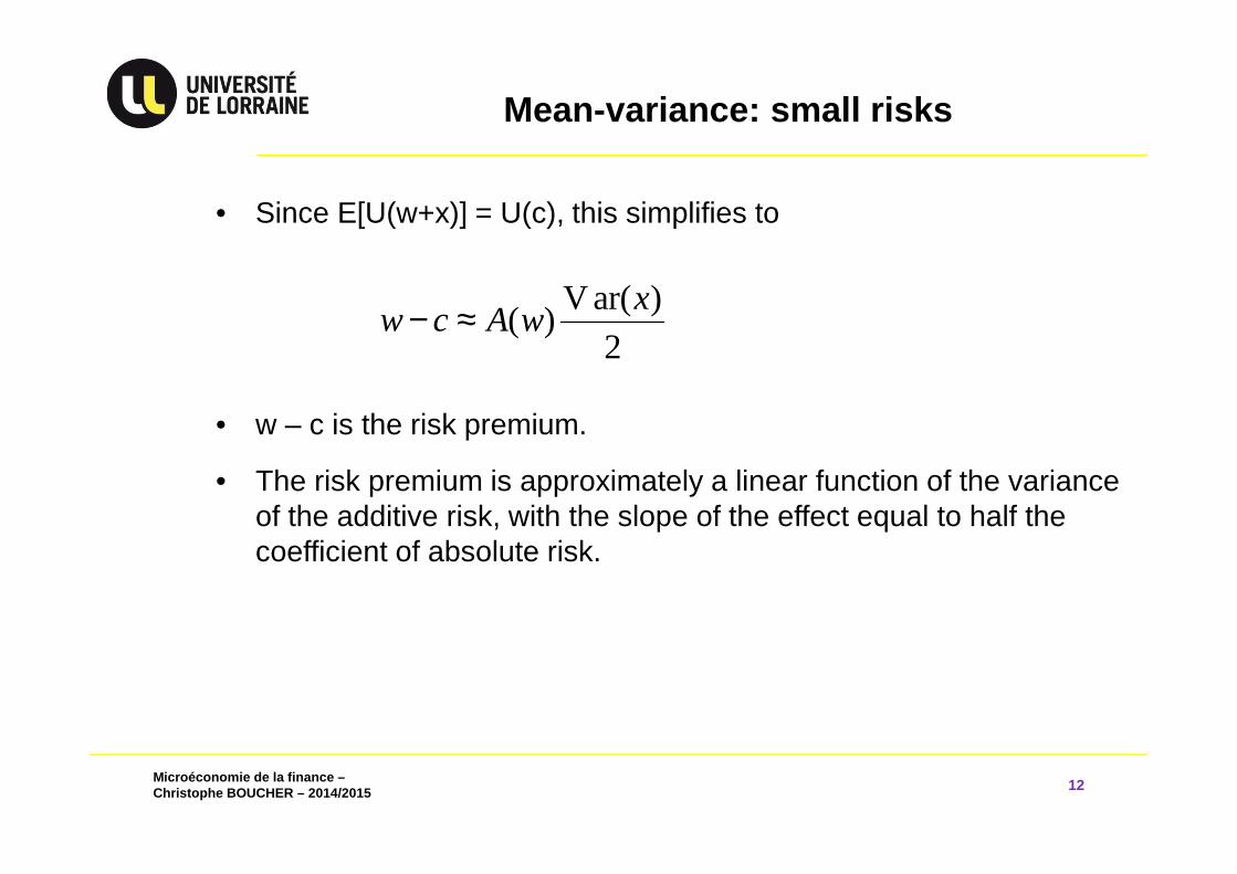
• Since E[U(w+x)] = U(c), this simplifies to
• w – c is the risk premium.
• The risk premium is approximately a linear function of the variance of the additive risk, with the slope of the effect equal to half the coefficient of absolute risk.
V ar( )( )
2
xw c A w− ≈
Microéconomie de la finance –Christophe BOUCHER – 2014/2015
Example: Simple mean-variance utility function
13
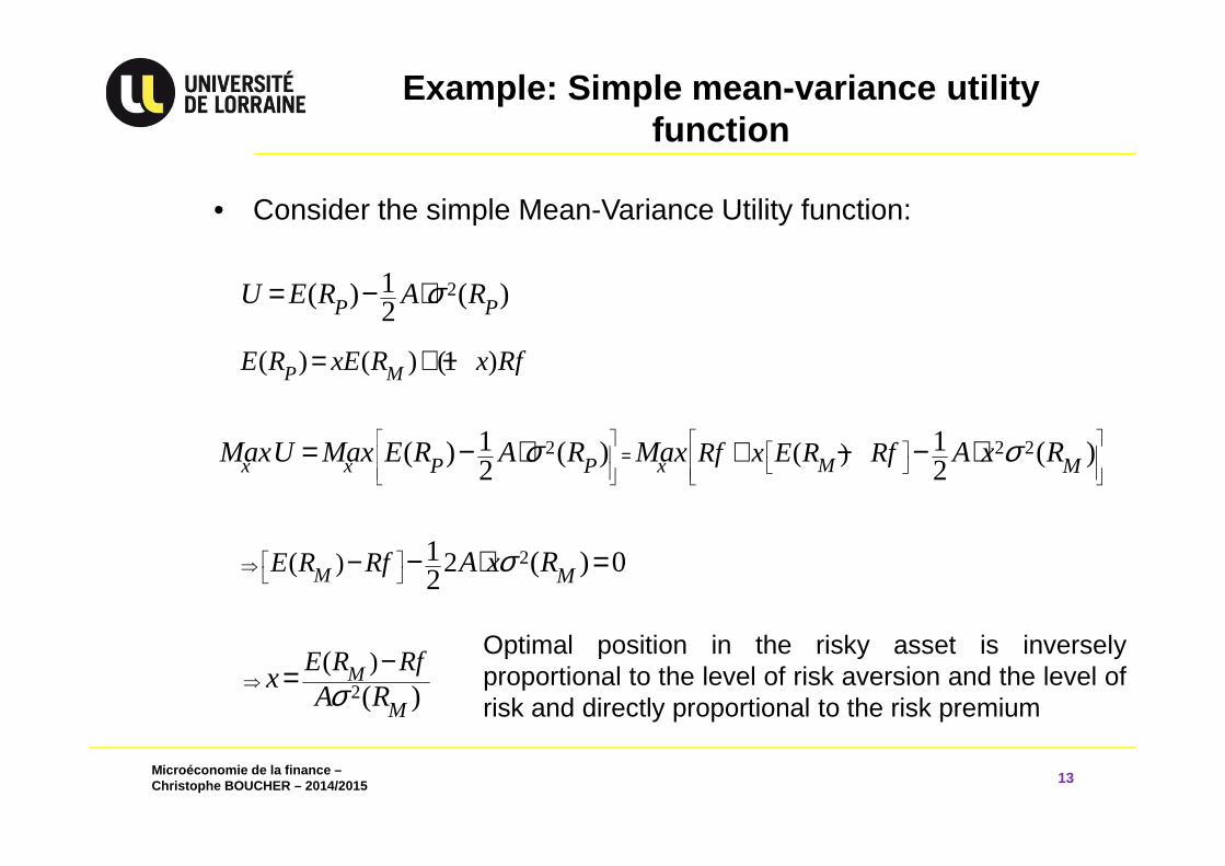
• Consider the simple Mean-Variance Utility function:
21( ) ( )2P PU E R A Rσ= − ⋅
2 2 2)(1 1( ) ( ) ( )2 2Mx x xP P MRf x E R RfMaxU Max E R A R Max A x Rσ σ
=
+ −= − ⋅ − ⋅
( ) ( ) (1 )P ME R xE R x Rf= + −
2)( 21 ( ) 02M ME R Rf A x Rσ ⇒
− − ⋅ =
2
)(( )
M
M
E R Rfx
A Rσ⇒−=
Optimal position in the risky asset is inverselyproportional to the level of risk aversion and the level ofrisk and directly proportional to the risk premium
Microéconomie de la finance –Christophe BOUCHER – 2014/2015
4.1 Measuring Risk and Return
14
Microéconomie de la finance –Christophe BOUCHER – 2014/2015
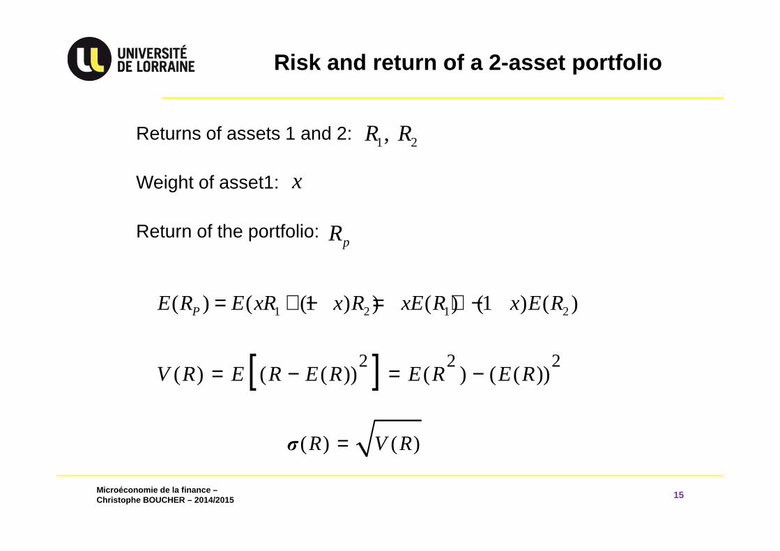
Returns of assets 1 and 2:
Weight of asset1:
Return of the portfolio:
Risk and return of a 2-asset portfolio
15
1 2, R R
x
pR
1 2 1 2( ) ( (1 ) ) ( ) (1 ) ( )PE R E xR x R xE R x E R= + − = + −
[ ]2 2 2( ) ( ( )) ( ) ( ( ))V R E R E R E R E R= − = −
( ) ( )R V Rσ =
Microéconomie de la finance –Christophe BOUCHER – 2014/2015
Risk and return of a 2-asset portfolio
16
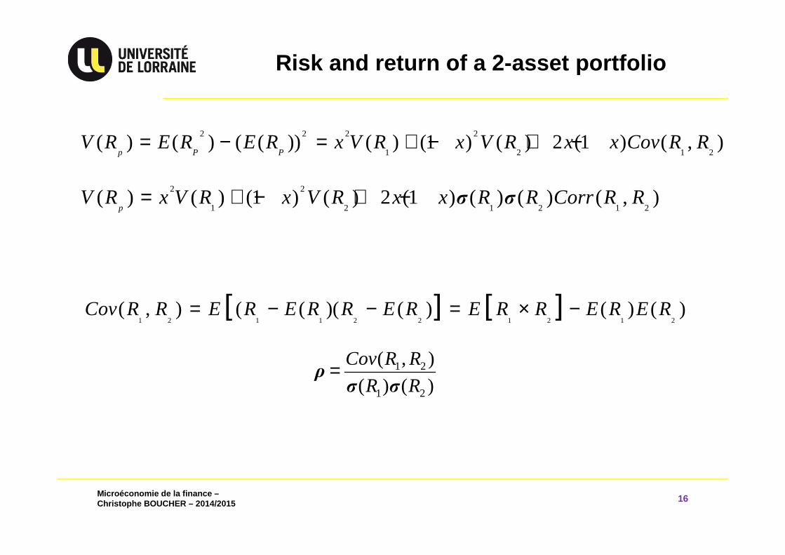
2 2 2 2
1 2 1 2( ) ( ) ( ( )) ( ) (1 ) ( ) 2 (1 ) ( , )
p P PV R E R E R x V R x V R x x Cov R R= − = + − + −
2 2
1 2 1 2 1 2( ) ( ) (1 ) ( ) 2 (1 ) ( ) ( ) ( , )
pV R x V R x V R x x R R Corr R Rσ σ= + − + −
[ ] [ ]1 2 1 1 2 2 1 2 1 2
( , ) ( ( )( ( ) ( ) ( )Cov R R E R E R R E R E R R E R E R= − − = × −
1 2
1 2
( , )
( ) ( )
Cov R R
R R=ρσ σ
Microéconomie de la finance –Christophe BOUCHER – 2014/2015
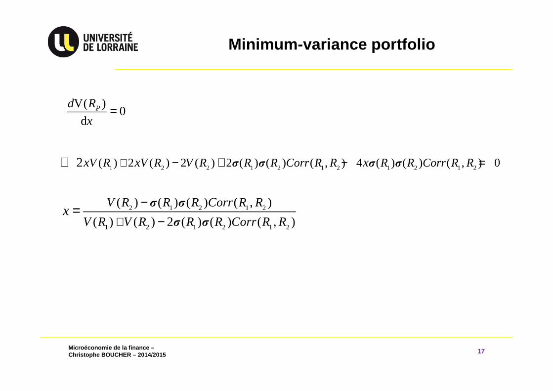
Minimum -variance portfolio
17
V( )0
dPd R
x=
1 2 2 1 2 1 2 1 2 1 2( ) 2 ( ) 2 ( ) 2 ( ) ( ) ( , ) 4 ( ) ( ) ( , ) 02 V R V R V R R R Corr R R R R Corr R Rx x xσ σ σ σ+ − + − =⇔
2 1 2 1 2
1 2 1 2 1 2
( ) ( ) ( ) ( , )
( ) ( ) 2 ( ) ( ) ( , )
V R R R Corr R R
V R V R R R Corr R Rx
σ σ
σ σ+
−−
=
Microéconomie de la finance –Christophe BOUCHER – 2014/2015
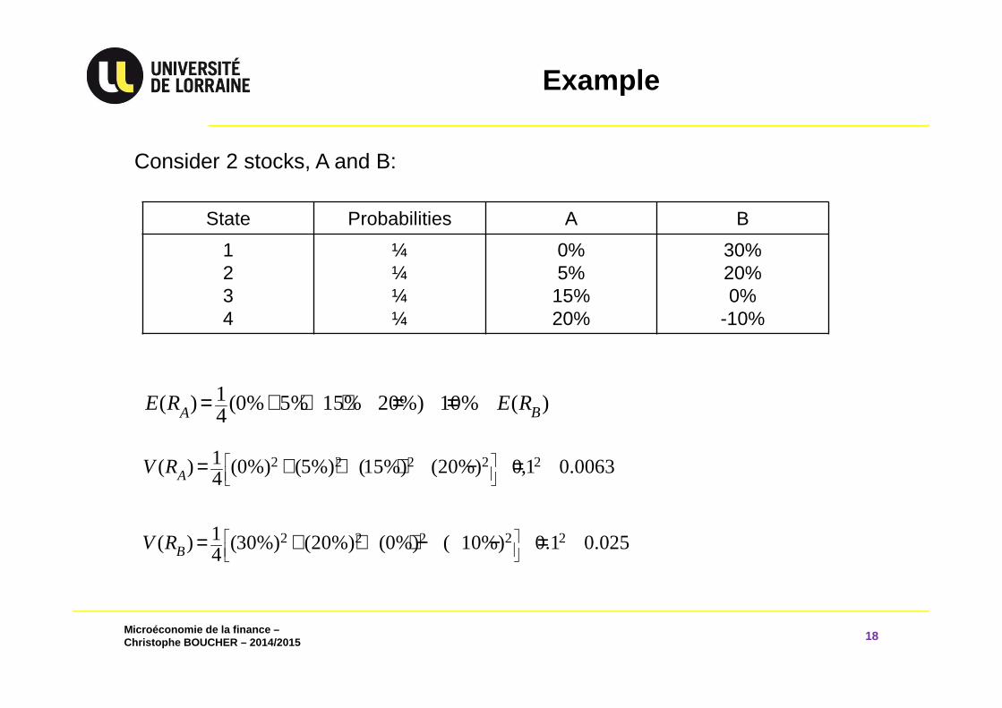
Example
18
Consider 2 stocks, A and B:
State Probabilities A B
1234
¼¼¼¼
0%5%
15%20%
30%20%0%
-10%
1( ) (0% 5% 15% 20%) 10% ( )4 BAE R E R= + + + = =
2 2 2 2 21( ) (0%) (5%) (15%) (20%) 0,1 0.00634AV R
= + + + − =
2 2 2 2 21( ) (30%) (20%) (0%) ( 10%) 0.1 0.0254BV R
= + + + − − =
Microéconomie de la finance –Christophe BOUCHER – 2014/2015
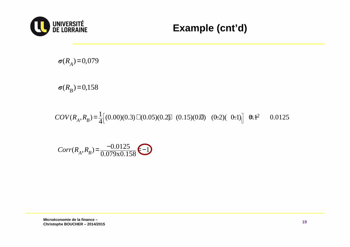
Example (cnt’d)
19
( ) 0,079AR =σ
( ) 0,158BR =σ
21( , ) (0.00)(0.3) (0.05)(0.2) (0.15)(0.0) (0.2)( 0.1) 0.1 0.01254BACOV R R
= + + + − − = −
0.0125( , ) 10.079x0.158BACorr R R −= = −
Microéconomie de la finance –Christophe BOUCHER – 2014/2015
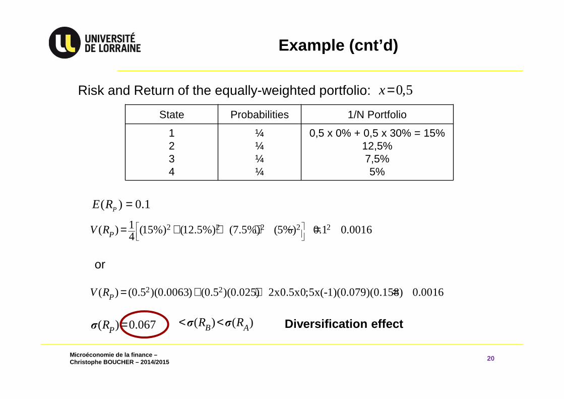
Example (cnt’d)
20
Risk and Return of the equally-weighted portfolio: 0,5x=
State Probabilities 1/N Portfolio
1234
¼¼¼¼
0,5 x 0% + 0,5 x 30% = 15%12,5%7,5%5%
( ) 0.1PE R =
2 2 2 2 21( ) (15%) (12.5%) (7.5%) (5%) 0.1 0.00164PV R
= + + + − =
or
2 2( ) (0.5 )(0.0063) (0.5 )(0.025) 2x0.5x0;5x(-1)(0.079)(0.158) 0.0016PV R = + + =
( ) 0.067PR =σ ( ) ( )B AR R< <σ σ Diversification effect
Microéconomie de la finance –Christophe BOUCHER – 2014/2015
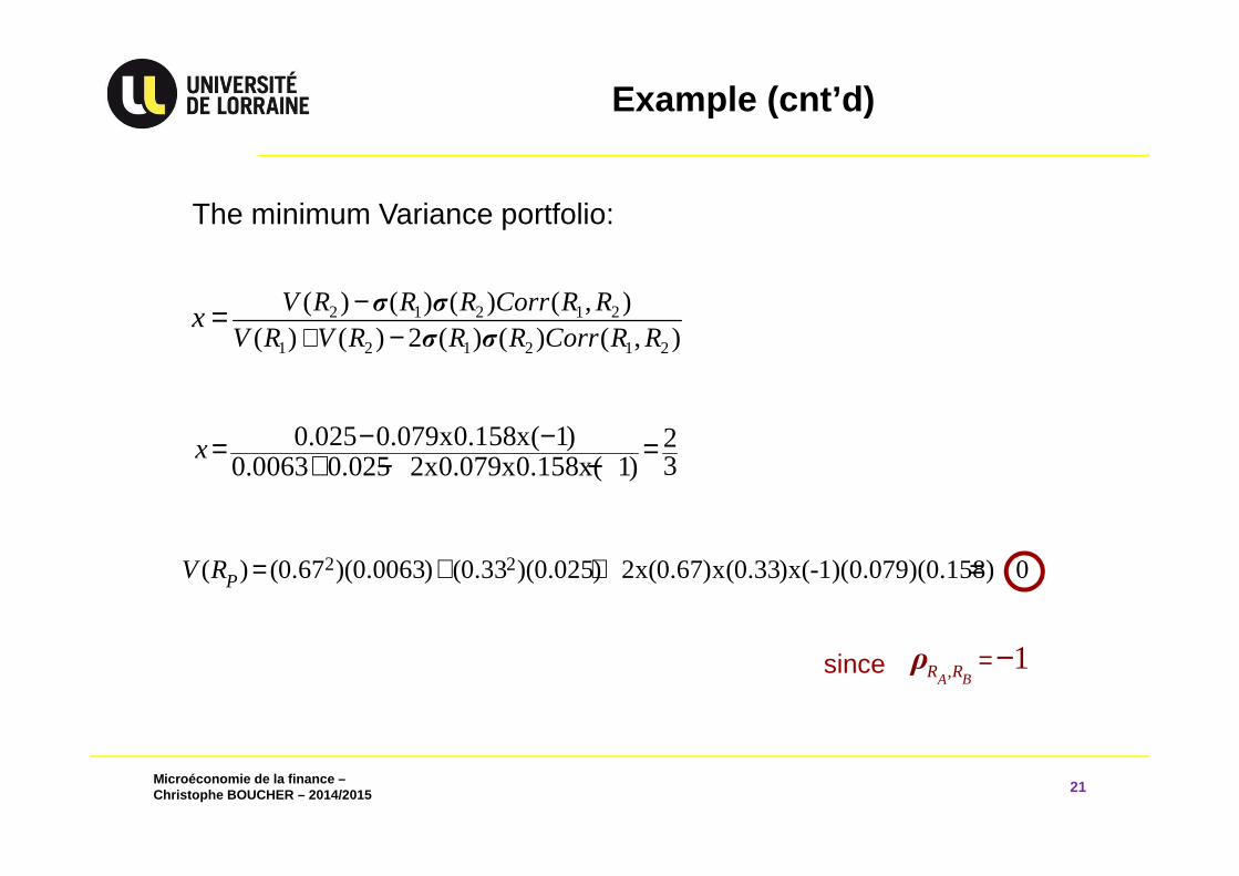
Example (cnt’d)
21
The minimum Variance portfolio:
2 1 2 1 2
1 2 1 2 1 2
( ) ( ) ( ) ( , )( ) ( ) 2 ( ) ( ) ( , )
V R R R Corr R RV R V R R R Corr R R
x+
−−
= σ σ
σ σ
0.025 0.079x0.158x( 1) 230.0063 0.025 2x0.079x0.158x( 1)
x − −= =+ − −
2 2( ) (0.67 )(0.0063) (0.33 )(0.025) 2x(0.67)x(0.33)x(-1)(0.079)(0.158) 0PV R = + + =
since , 1BAR R =−ρ
Microéconomie de la finance –Christophe BOUCHER – 2014/2015
4.2 Asset Allocation with 2 Risky Assets
22
Microéconomie de la finance –Christophe BOUCHER – 2014/2015
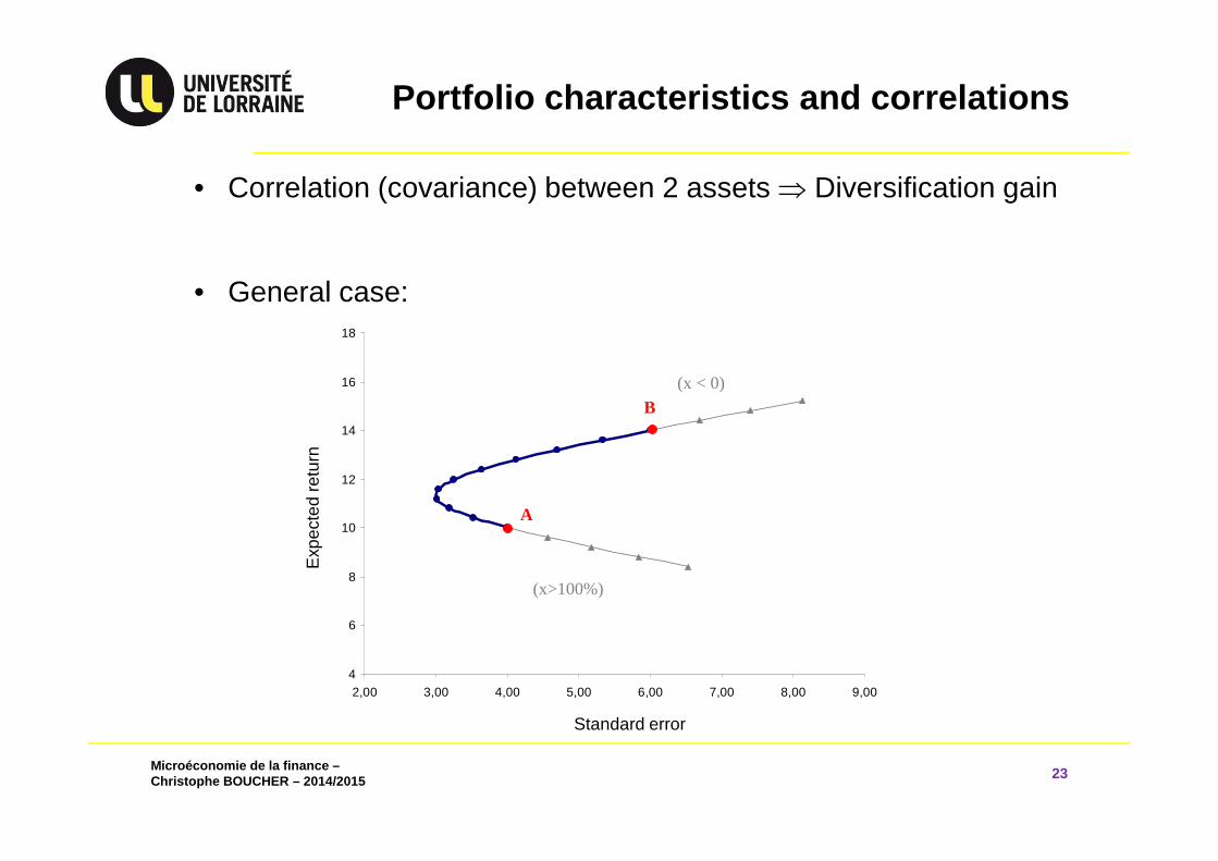
Portfolio characteristics and correlations
23
• Correlation (covariance) between 2 assets ⇒ Diversification gain
• General case:
4
6
8
10
12
14
16
18
2,00 3,00 4,00 5,00 6,00 7,00 8,00 9,00
A
B
(x>100%)
(x < 0)
4
6
8
10
12
14
16
18
2,00 3,00 4,00 5,00 6,00 7,00 8,00 9,004
6
8
10
12
14
16
18
2,00 3,00 4,00 5,00 6,00 7,00 8,00 9,00
A
B
(x>100%)
(x < 0)
Exp
ecte
d re
turn
Standard error
Microéconomie de la finance –Christophe BOUCHER – 2014/2015
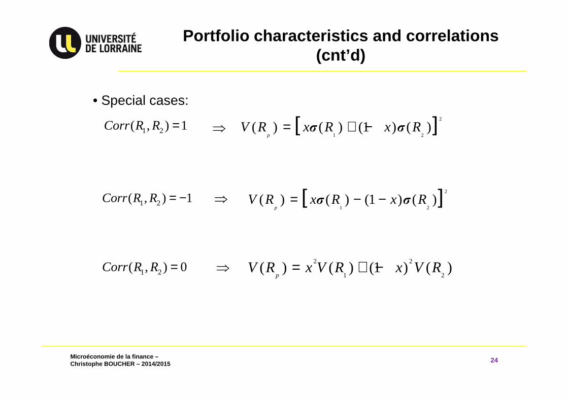
Portfolio characteristics and correlations (cnt’d)
24
• Special cases:
1 2( , ) 1Corr R R =
1 2( , ) 1Corr R R = −
1 2( , ) 0Corr R R =
[ ]2
1 2( ) ( ) (1 ) ( )
pV R x R x R= + −σ σ⇒
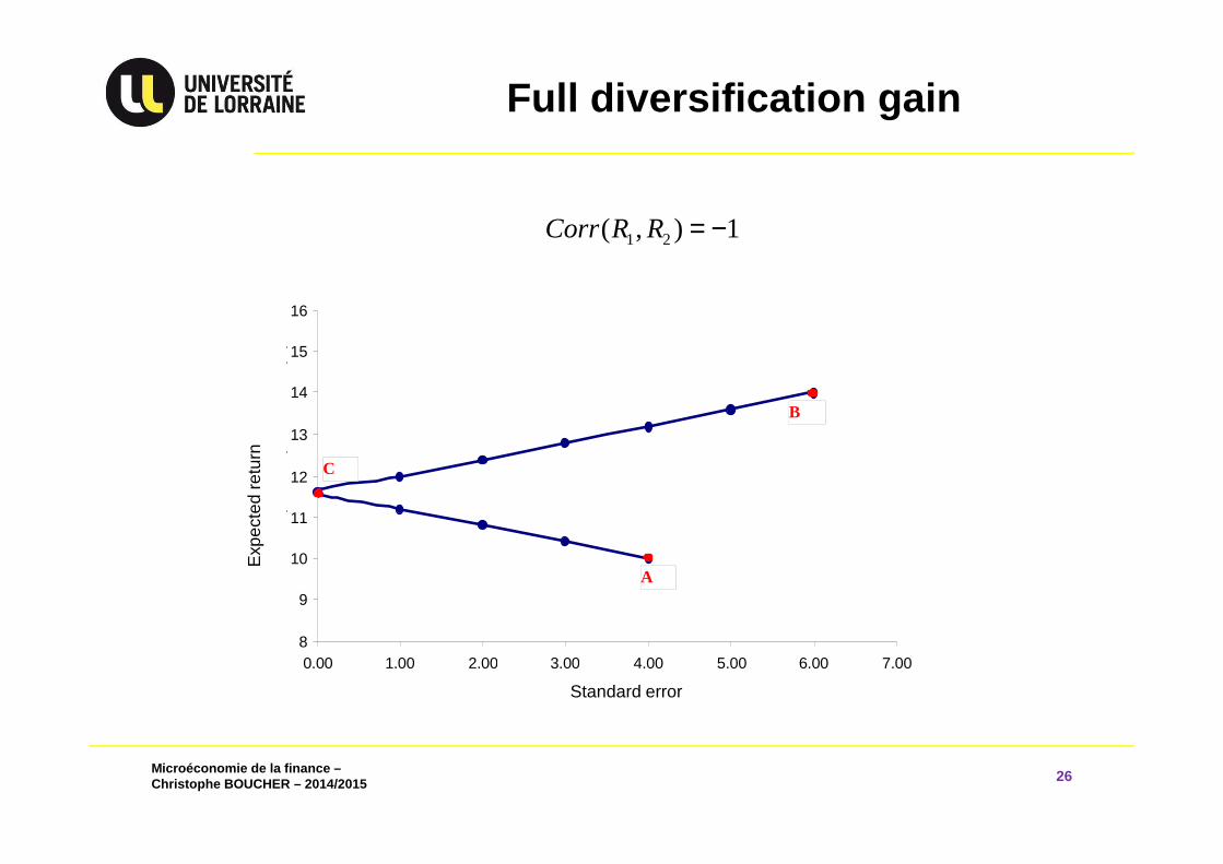
[ ]2
1 2( ) ( ) (1 ) ( )
pV R x R x Rσ σ= − −⇒
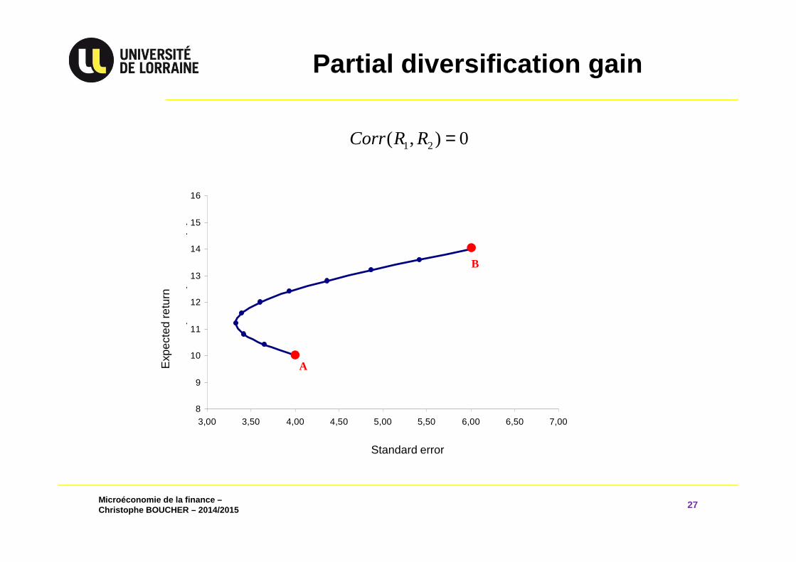
2 2
1 2( ) ( ) (1 ) ( )
pV R x V R x V R= + −⇒
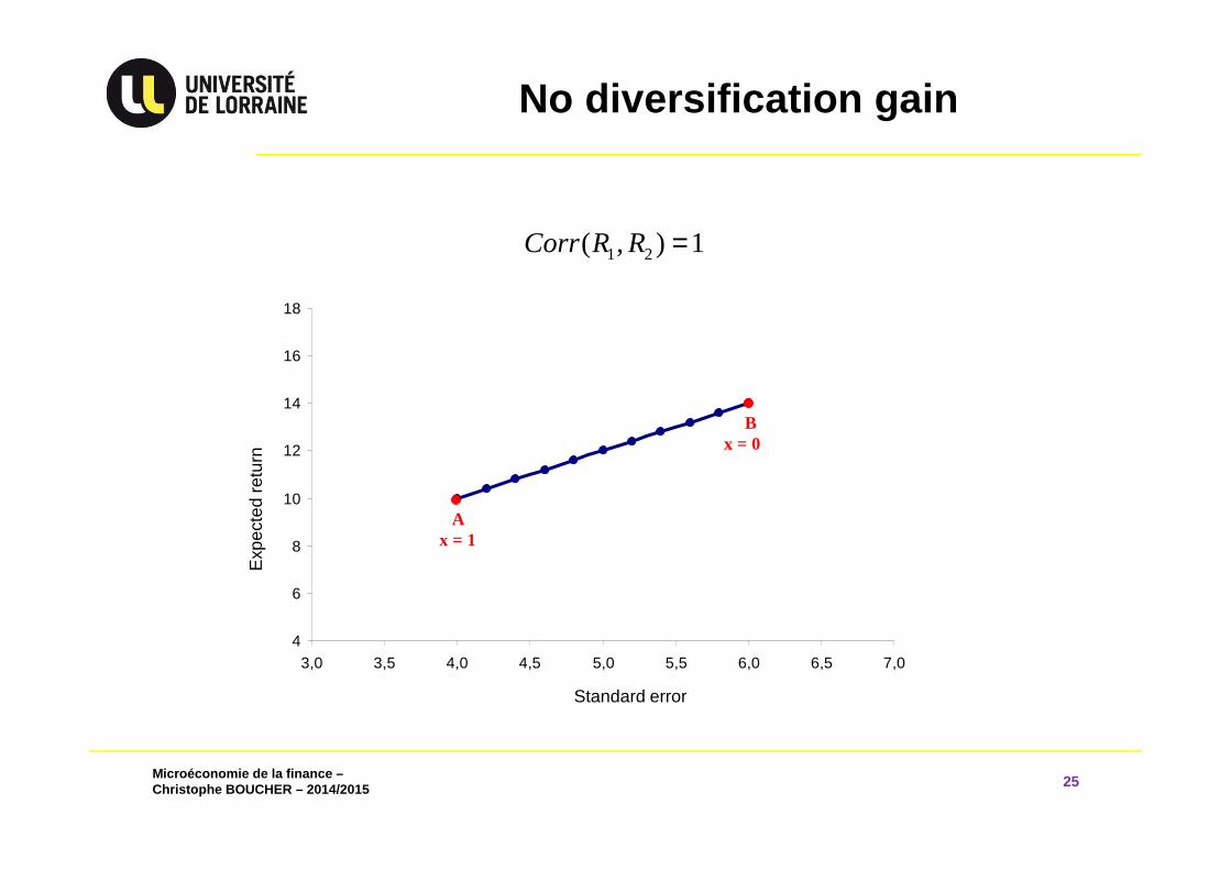
Microéconomie de la finance –Christophe BOUCHER – 2014/2015
No diversification gain
25
1 2( , ) 1Corr R R =
4
6
8
10
12
14
16
18
3,0 3,5 4,0 4,5 5,0 5,5 6,0 6,5 7,0
Ren
dem
ent e
spér
é du
por
tefe
uille
(%
)
A
B
x = 1
x = 0
Exp
ecte
d re
turn
Standard error
Microéconomie de la finance –Christophe BOUCHER – 2014/2015
Full diversification gain
26
1 2( , ) 1Corr R R = −E
xpec
ted
retu
rn
Standard error
8
9
10
11
12
13
14
15
16
0,00 1,00 2,00 3,00 4,00 5,00 6,00 7,00Ecart type du portefeuille (%)
Ren
dem
ent e
spér
é du
por
tefe
uille
(%
)
A
B
C
Microéconomie de la finance –Christophe BOUCHER – 2014/2015
Partial diversification gain
27
1 2( , ) 0Corr R R =E
xpec
ted
retu
rn
Standard error
8
9
10
11
12
13
14
15
16
3,00 3,50 4,00 4,50 5,00 5,50 6,00 6,50 7,00
Ren
dem
ent e
spér
é du
por
tefe
uille
(%
)
A
B
Microéconomie de la finance –Christophe BOUCHER – 2014/2015
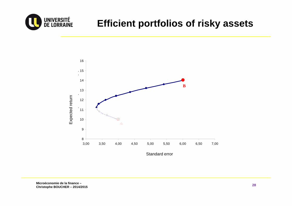
Efficient portfolios of risky assets
28
Exp
ecte
d re
turn
Standard error
8
9
10
11
12
13
14
15
16
3,00 3,50 4,00 4,50 5,00 5,50 6,00 6,50 7,00
Ren
dem
ent e
spér
é du
por
tefe
uille
(%
)
A
B
Microéconomie de la finance –Christophe BOUCHER – 2014/2015
4.3 Introducing a Risk Free Asset and the Tobin’s Separation Theorem
29
Microéconomie de la finance –Christophe BOUCHER – 2014/2015
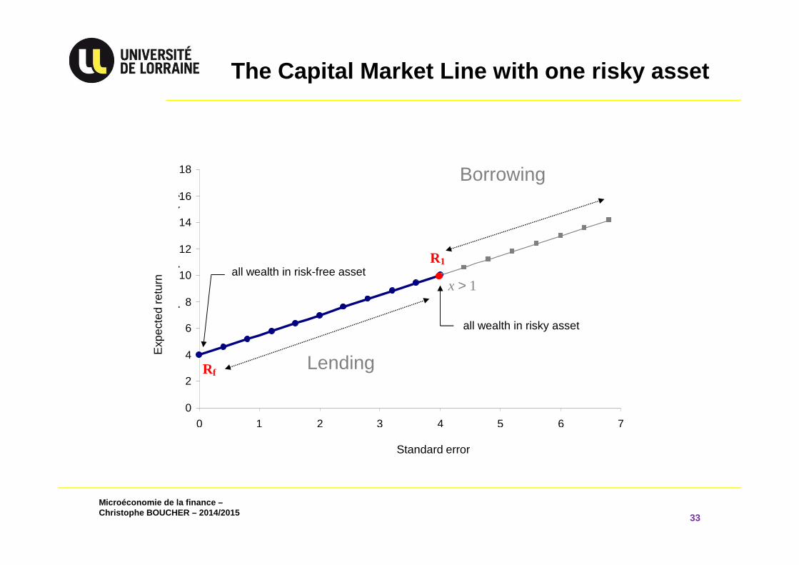
Introducing borrowing and lending:Risk free asset
30
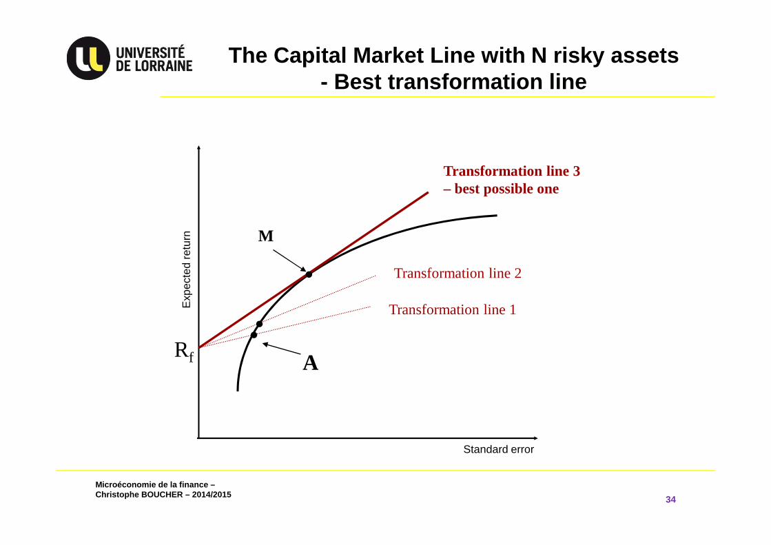
• You are now allowed to borrow and lend at the risk free rate Rf while still investing in any SINGLE ‘risky bundle’ on the efficient frontier.
• For each SINGLE risky bundle, this gives a new set of risk return combination known as the ‘transformation line’.
• The risk-return combination is a straight line (for each single risky bundle) - transformation line.
• You can be anywhere you like on this line.
Microéconomie de la finance –Christophe BOUCHER – 2014/2015
The risk free asset
31
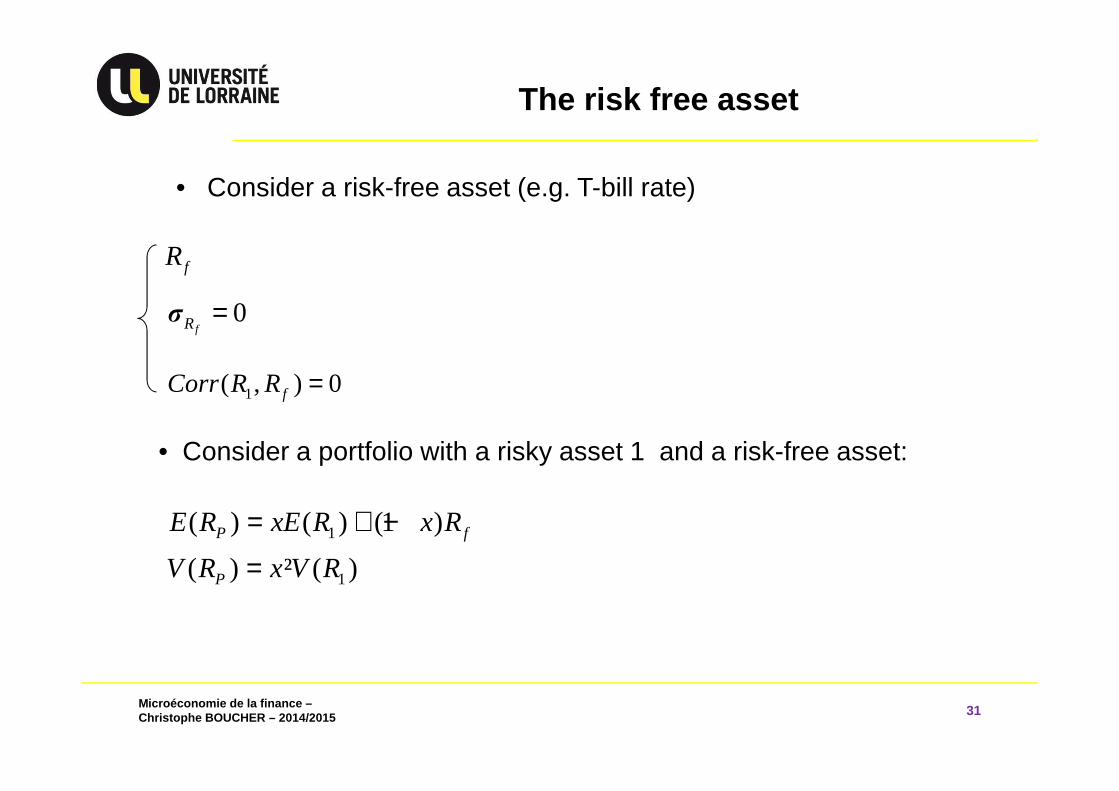
• Consider a risk-free asset (e.g. T-bill rate)
fR
0fRσ =
1( , ) 0fCorr R R =
• Consider a portfolio with a risky asset 1 and a risk-free asset:
1
1
( ) ( ) (1 )
( ) ² ( )P f
P
E R xE R x R
V R x V R
= + −
=
Microéconomie de la finance –Christophe BOUCHER – 2014/2015
The Capital Market Line
32
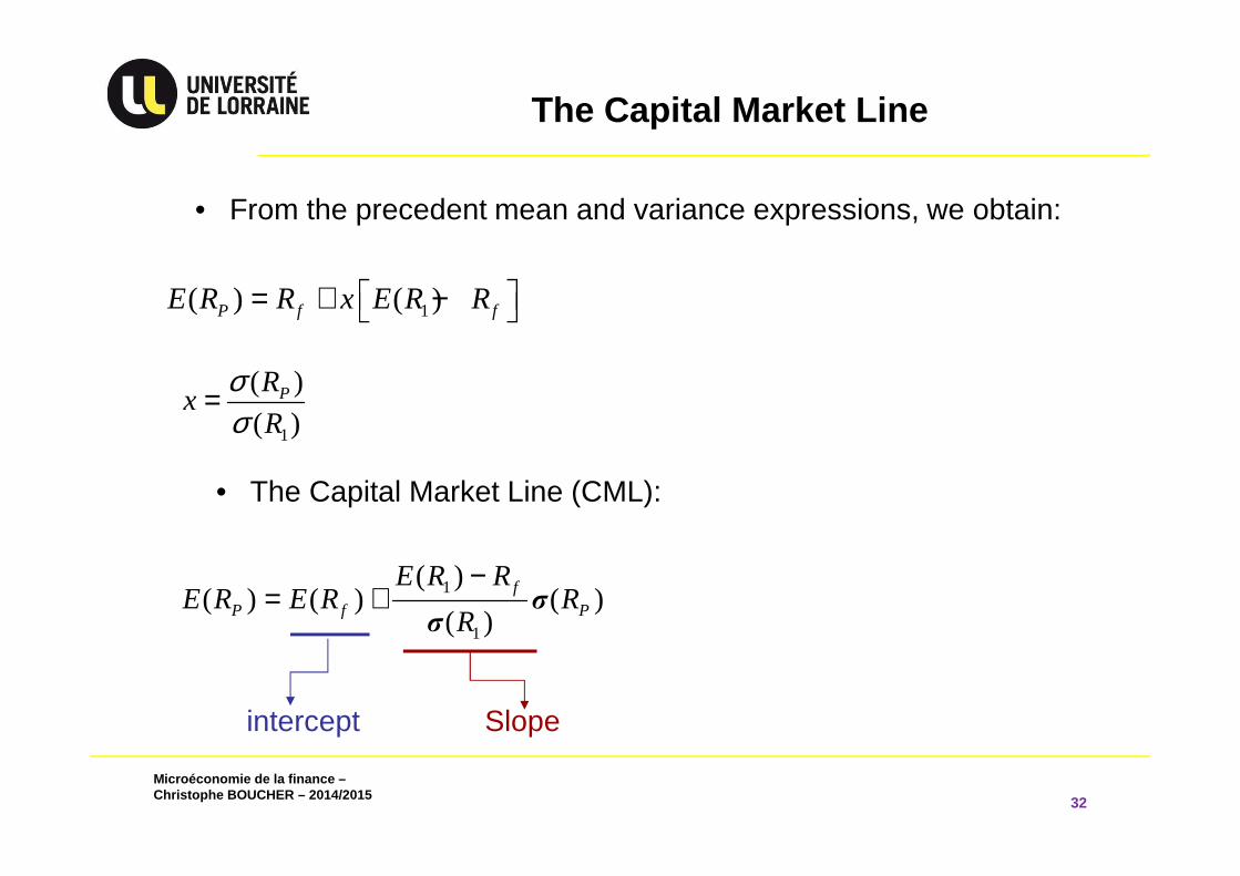
• From the precedent mean and variance expressions, we obtain:
1( ) ( )P f fE R R x E R R = + −
1
( )
( )PR
xR
σσ
=
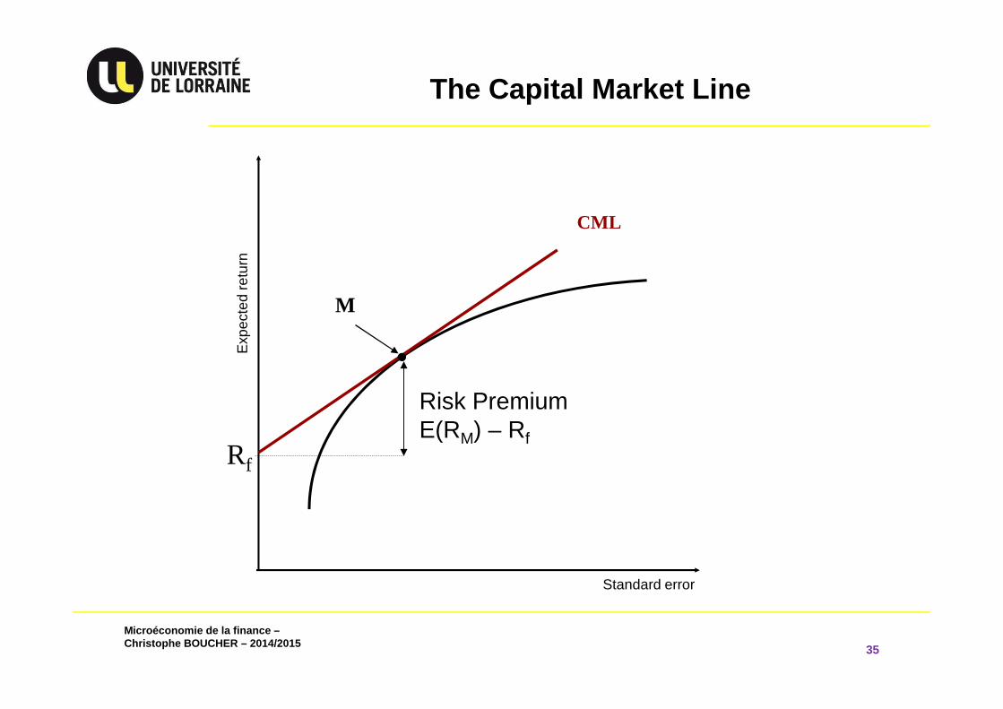
• The Capital Market Line (CML):
1
1
( )( ) ( ) ( )
( )f
P f P
E R RE R E R R
R
−= + σ
σ
Slopeintercept
Microéconomie de la finance –Christophe BOUCHER – 2014/2015
The Capital Market Line with one risky asset
33
0
2
4
6
8
10
12
14
16
18
0 1 2 3 4 5 6 7
Ren
dem
ent e
spér
é du
por
tefe
uille
(%
)
R1
Rf
x > 1
all wealth in risky asset
Exp
ecte
d re
turn
Standard error
all wealth in risk-free asset
Lending
Borrowing
Microéconomie de la finance –Christophe BOUCHER – 2014/2015
The Capital Market Line with N risky assets- Best transformation line
34
Exp
ecte
d re
turn
Standard error
Transformation line 1
Transformation line 2
Transformation line 3 – best possible one
Rf A
M
Microéconomie de la finance –Christophe BOUCHER – 2014/2015
The Capital Market Line
35
Exp
ecte
d re
turn
Standard error
CML
Rf
M
Risk PremiumE(RM) – Rf
Microéconomie de la finance –Christophe BOUCHER – 2014/2015
The CML and the separation theorem
36
• The CML dominates all other possible portfolios
• An agent invests along the CML (where ? ⇒ risk preferences)
• James Tobin’s separation theorem:
- Invest in a risky portfolio (optimal combination of risky securities)
- Borrow-lend at the risk-free rate
• Depending on your attitude toward risk: how much lend or borrow
Microéconomie de la finance –Christophe BOUCHER – 2014/2015
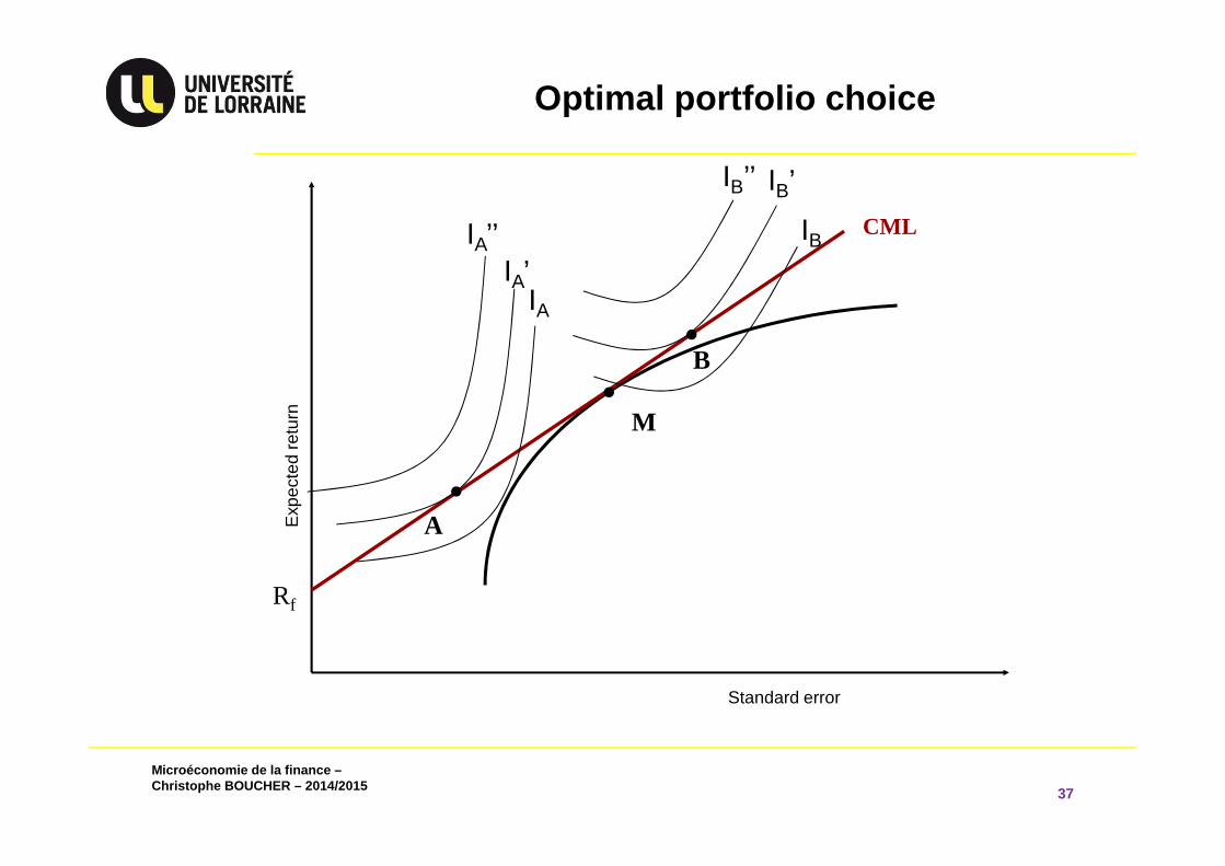
Optimal portfolio choice
37
Exp
ecte
d re
turn
CML
Rf
M
Standard error
A
B
IA’IA’’ IB
IA
IB’’ IB’
Microéconomie de la finance –Christophe BOUCHER – 2014/2015
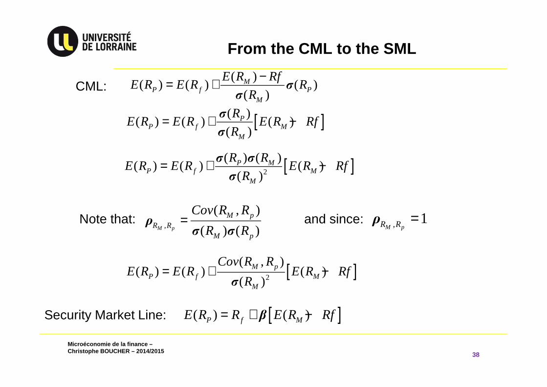
From the CML to the SML
38
( )( ) ( ) ( )
( )M
P f PM
E R RfE R E R R
R
−= + σσ
CML:
[ ]( )( ) ( ) ( )
( )P
P f MM
RE R E R E R Rf
R= + −σ
σ
Note that:,
( , )
( ) ( )M p
M pR R
M p
Cov R R
R R=ρσ σ
and since: , 1M pR R =ρ
[ ]2
( ) ( )( ) ( ) ( )
( )P M
P f MM
R RE R E R E R Rf
R= + −σ σ
σ
[ ]2
( , )( ) ( ) ( )
( )M p
P f MM
Cov R RE R E R E R Rf
R= + −
σ
Security Market Line: [ ]( ) ( )P f ME R R E R Rf= + −β
Microéconomie de la finance –Christophe BOUCHER – 2014/2015
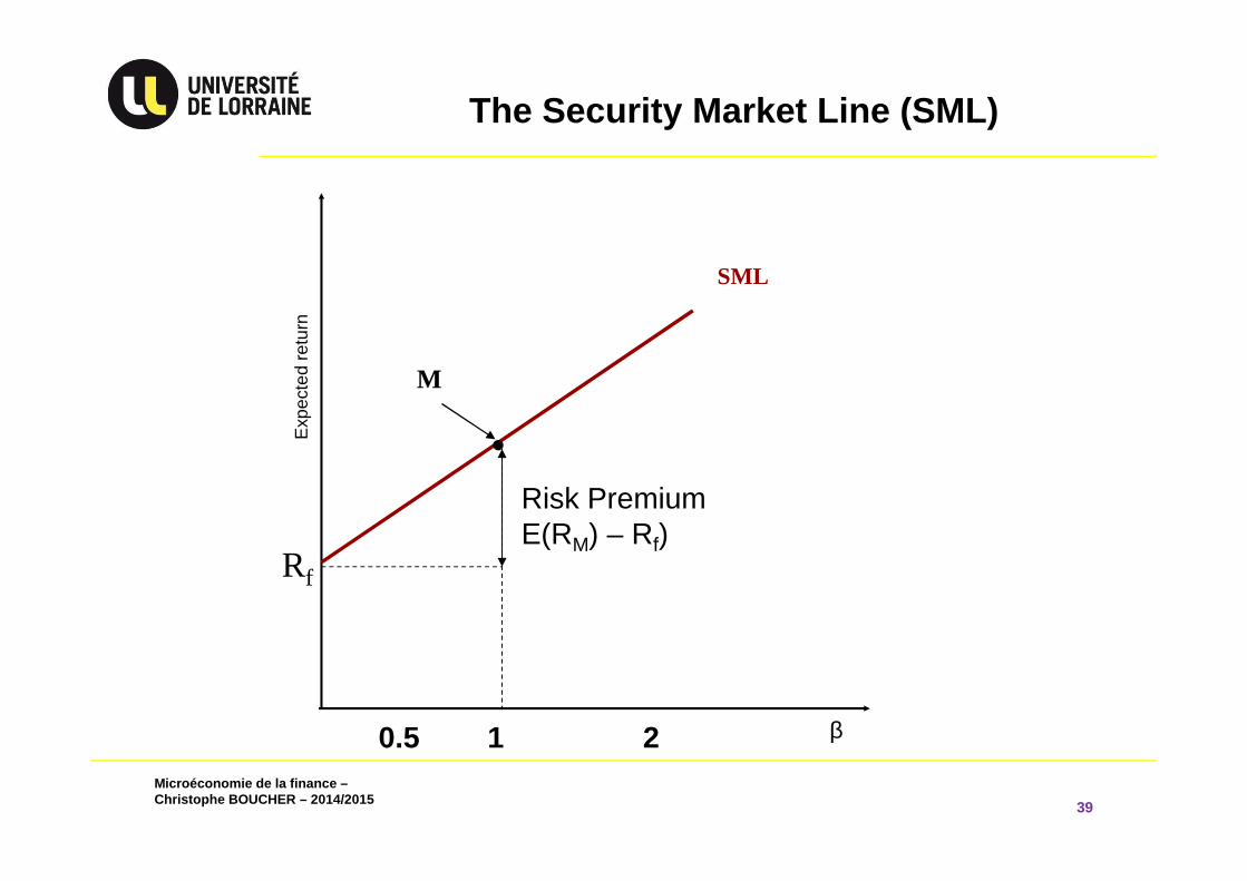
The Security Market Line (SML)
39
Exp
ecte
d re
turn
SML
Rf
M
β10.5 2
Risk PremiumE(RM) – Rf)
Microéconomie de la finance –Christophe BOUCHER – 2014/2015
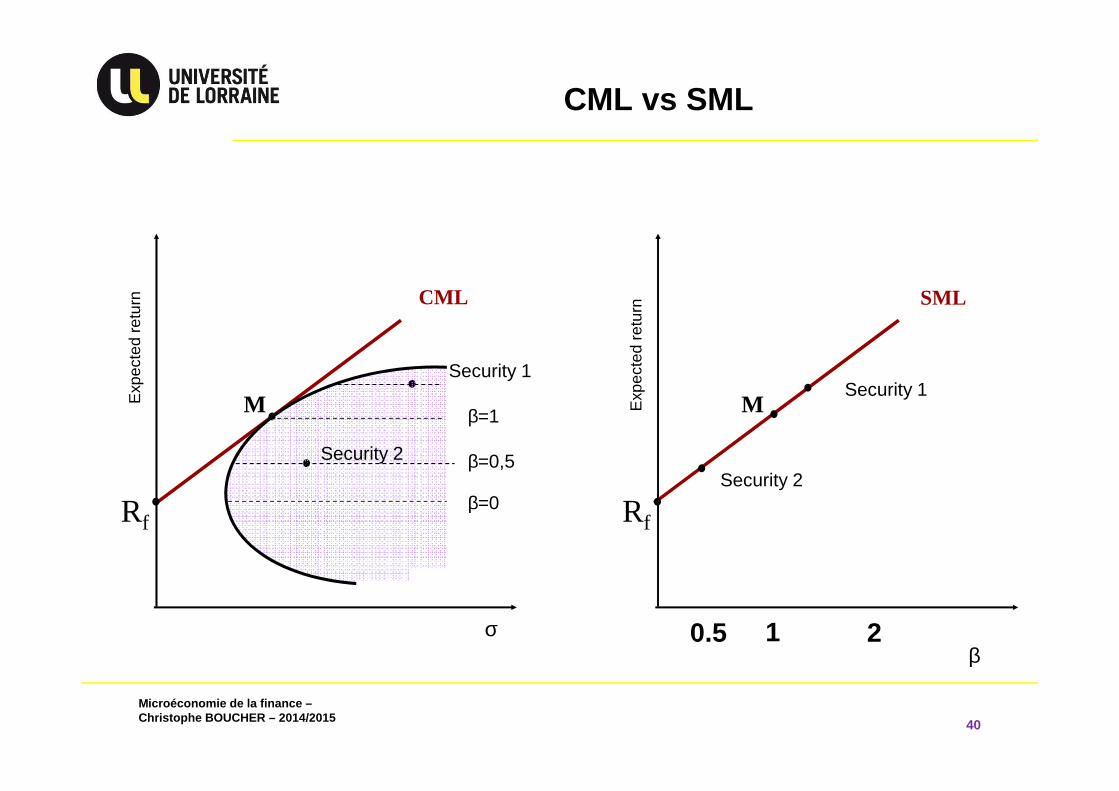
CML vs SML
40
βE
xpec
ted
retu
rn SML
Rf
M
10.5 2
Security 1
Security 2
σ
Exp
ecte
d re
turn CML
Rf
M
Security 2
Security 1
β=0
β=0,5
β=1
Microéconomie de la finance –Christophe BOUCHER – 2014/2015
CML vs SML
41
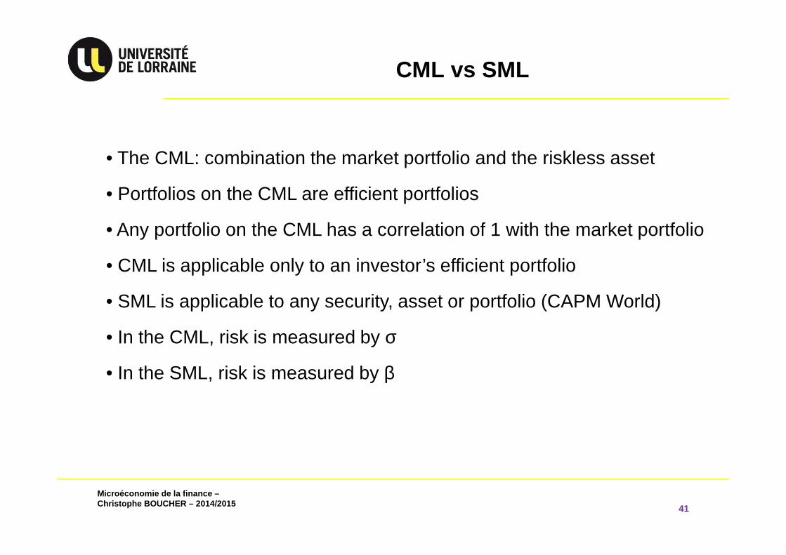
• The CML: combination the market portfolio and the riskless asset
• Portfolios on the CML are efficient portfolios
• Any portfolio on the CML has a correlation of 1 with the market portfolio
• CML is applicable only to an investor’s efficient portfolio
• SML is applicable to any security, asset or portfolio (CAPM World)
• In the CML, risk is measured by σ
• In the SML, risk is measured by β

Microéconomie de la finance –Christophe BOUCHER – 2014/2015
4.4 Asset Allocation with N risky Assets
42
Microéconomie de la finance –Christophe BOUCHER – 2014/2015
Efficient portfolios
43
• Efficient portfolios are those that maximize the ex pected return for a given level of expected risk
• or minimize the risk for a given level of expected return
• Two kinds of efficient portfolios:
- only risky assets
- both risky assets and a riskless-asset (separation theorem)
• Suppose stable expected-returns and VCV matrix
Microéconomie de la finance –Christophe BOUCHER – 2014/2015
Some notations
44
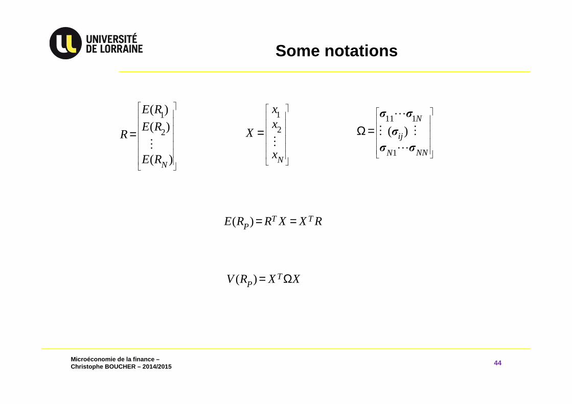
1
2
( )
( )
( )N
E R
E RR
E R
=⋮
1
2
N
xx
X
x
=⋮
11 1
1
( )N
ij
NNN
Ω =⋯
⋮ ⋮
⋯
σ σ
σ
σ σ
( ) T TPE R R X X R= =
( ) TPV R X X= Ω
Microéconomie de la finance –Christophe BOUCHER – 2014/2015
Efficient frontier with a riskless asset
45
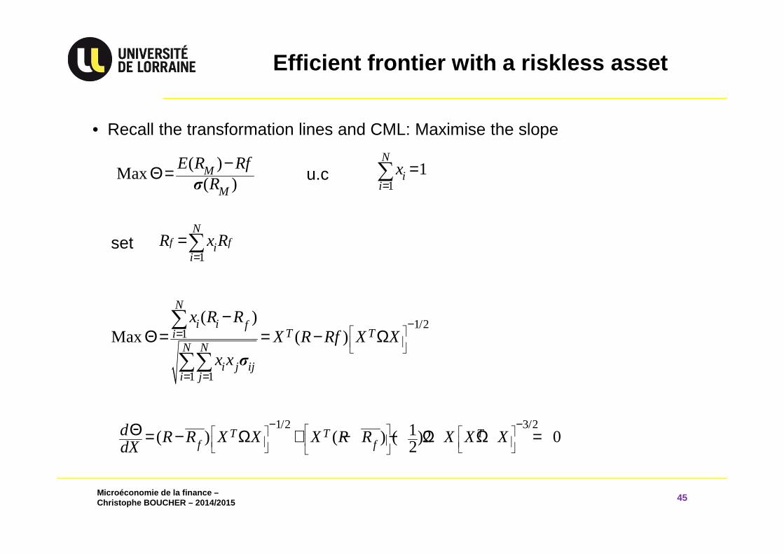
( )Max
( )M
M
E R RfR
−Θ =σ
• Recall the transformation lines and CML: Maximise the slope
11
N
ii
x=
=∑u.c
1f f
N
ii
R x R=
=∑set
1/21
1 1
( )Max ( )
N
i i fT Ti
N N
i j iji j
x R RX R Rf X X
x x
−=
= =
−Θ = = − Ω
∑
∑∑ σ
1/2 3/21( ) ( ) ( )2 02
T T Tf f
d R R X X X R R X X XdX
− −Θ = − Ω + − − Ω Ω =
Microéconomie de la finance –Christophe BOUCHER – 2014/2015
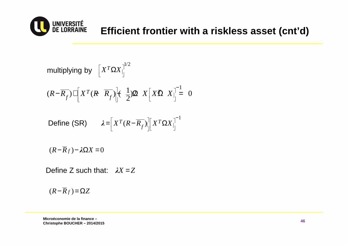
Efficient frontier with a riskless asset (cnt’d)
46
multiplying by1/2
TX X
Ω
11( ) ( ) ( )2 02
T Tf fR R X R R X X X
−− + − − Ω Ω =
1( )T T
fX R R X X
−= − ΩλDefine (SR)
( ) 0fR R X− − Ω =λ
X Z=λ
( )fR R Z− = Ω
Define Z such that:
Microéconomie de la finance –Christophe BOUCHER – 2014/2015
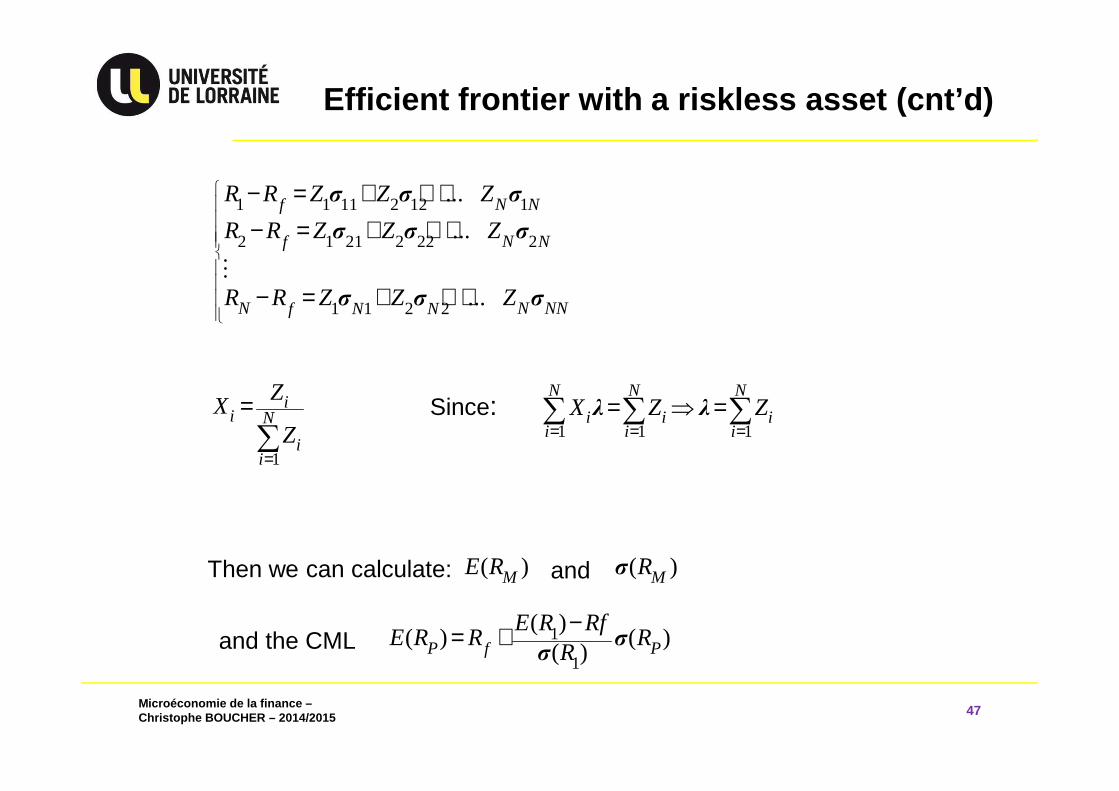
Efficient frontier with a riskless asset (cnt’d)
47
1 1 11 2 12 1
2 1 21 2 22 2
1 1 2 2
...
...
...
N Nf
N Nf
N N NNN Nf
R R Z Z Z
R R Z Z Z
R R Z Z Z
− = + + +− = + + +
− = + + +⋮
σ σ σ
σ σ σ
σ σ σ
1
ii N
ii
ZX
Z=
=∑
Since: 1 1 1
N N N
i i ii i i
X Z Z= = =
= ⇒ =∑ ∑ ∑λ λ
Then we can calculate: ( )ME R ( )MRσand
1
1
( )( ) ( )
( )P Pf
E R RfE R R R
R−= + σ
σand the CML
Microéconomie de la finance –Christophe BOUCHER – 2014/2015
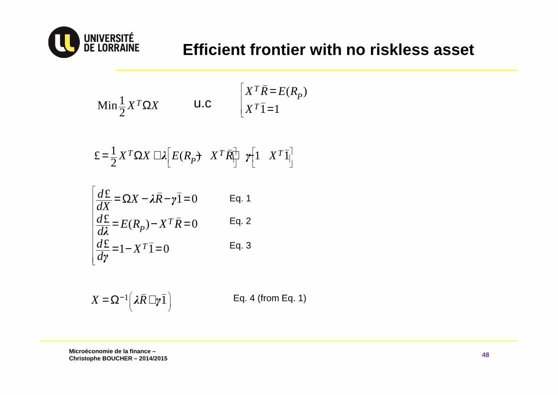
Efficient frontier with no riskless asset
48
1Min2
TX XΩ( )
1 1
TP
T
X R E R
X
==u.c
1£ ( ) 1 12
T T TPX X E R X R X
= Ω + − + −λ γ
£ 1 0
£ ( ) 0
£ 1 1 0
TP
T
d X RdXd E R X Rdd Xd
=Ω − − =
= − =
= − =
λ γ
λ
γ
1 1X R
−= Ω +λ γ
Eq. 1
Eq. 2
Eq. 3
Eq. 4 (from Eq. 1)
Microéconomie de la finance –Christophe BOUCHER – 2014/2015
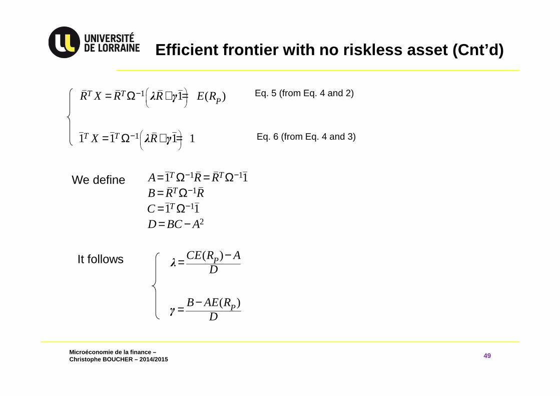
Efficient frontier with no riskless asset (Cnt’d)
49
1 1 ( )T TPR X R R E R
−= Ω + =λ γ
11 1 1 1T TX R
−= Ω + =λ γ
1 1
1
1
2
1 1
1 1
T T
T
T
A R RB R RCD BC A
− −
−
−
= Ω = Ω= Ω= Ω= −
We define
( )PCE R AD
−=λ
( )PB AE RD
−=γ
Eq. 5 (from Eq. 4 and 2)
Eq. 6 (from Eq. 4 and 3)
It follows
Microéconomie de la finance –Christophe BOUCHER – 2014/2015
Efficient frontier with no riskless asset (Cnt’d)
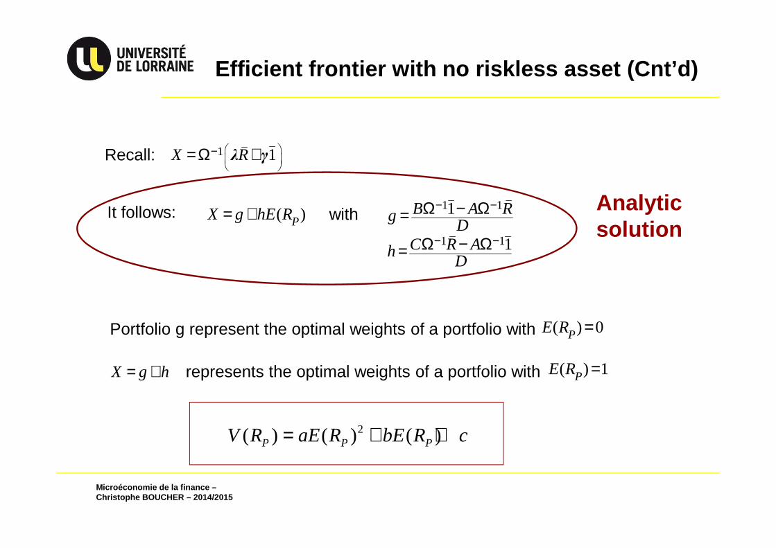
Recall: 1 1X R
−= Ω +λ γ
( )PX g hE R= + 1 1
1 1
1
1
B A RgD
C R AhD
− −
− −
Ω − Ω=
Ω − Ω=
with
Portfolio g represent the optimal weights of a portfolio with ( ) 0PE R =
X g h= + represents the optimal weights of a portfolio with ( ) 1PE R =
2( ) ( ) ( )P P PV R aE R bE R c= + +
It follows: Analytic solution
Microéconomie de la finance –Christophe BOUCHER – 2014/2015
Characterization of frontier portfolios
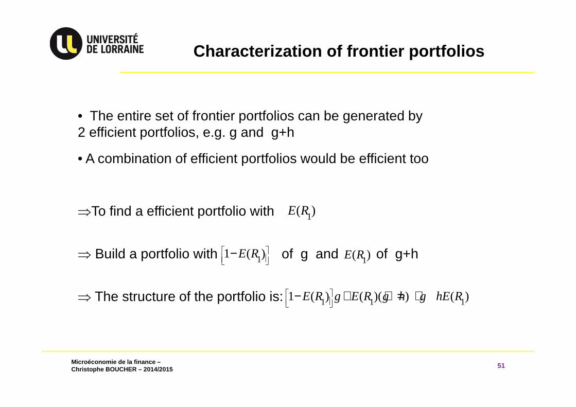
51
• The entire set of frontier portfolios can be generated by 2 efficient portfolios, e.g. g and g+h
• A combination of efficient portfolios would be efficient too
⇒To find a efficient portfolio with
⇒ Build a portfolio with of g and of g+h
⇒ The structure of the portfolio is:
1( )E R
11 ( )E R
−1( )E R
1 1 11 ( ) ( )( ) ( )E R g E R g h g hE R
− + + = +

Microéconomie de la finance –Christophe BOUCHER – 2014/2015
3.5 Portfolio Diversification
52
Microéconomie de la finance –Christophe BOUCHER – 2014/2015
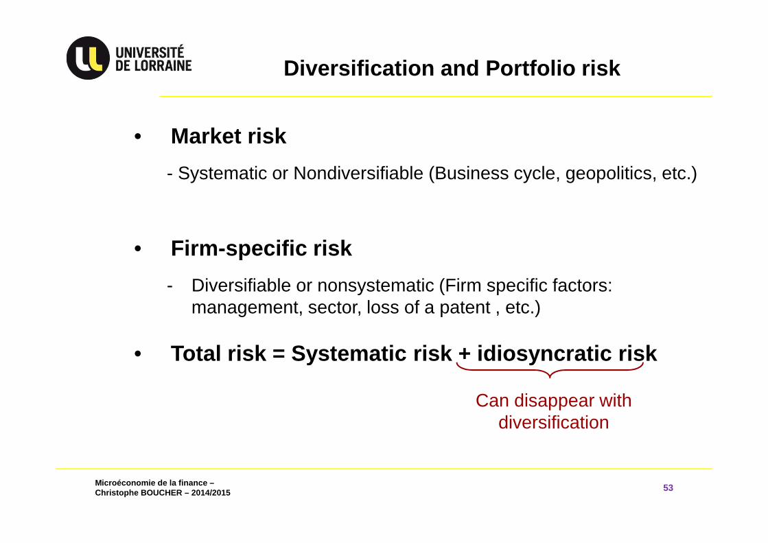
Diversification and Portfolio risk
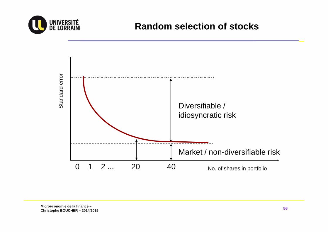
53
• Market risk
- Systematic or Nondiversifiable (Business cycle, geopolitics, etc.)
• Firm -specific risk
- Diversifiable or nonsystematic (Firm specific factors: management, sector, loss of a patent , etc.)
• Total risk = Systematic risk + idiosyncratic risk
Can disappear with diversification
Microéconomie de la finance –Christophe BOUCHER – 2014/2015
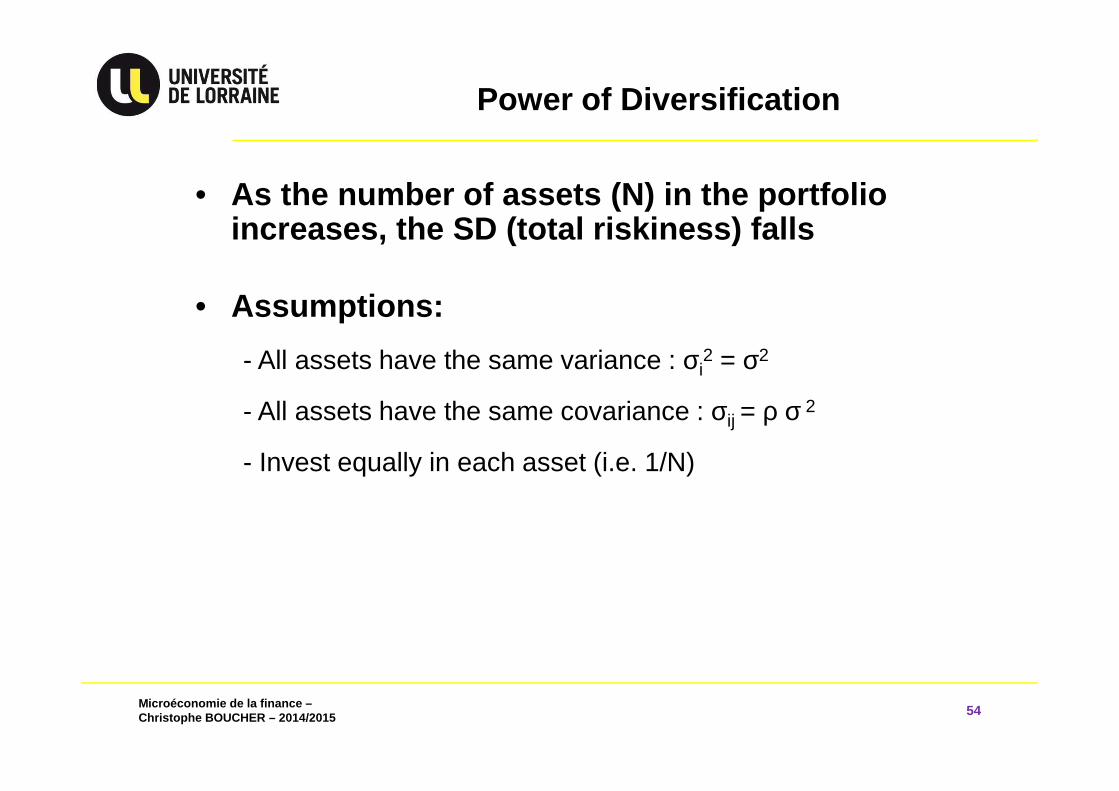
Power of Diversification
54
• As the number of assets (N) in the portfolio increases, the SD (total riskiness) falls
• Assumptions:
- All assets have the same variance : σi2 = σ2
- All assets have the same covariance : σij = ρ σ 2
- Invest equally in each asset (i.e. 1/N)
Microéconomie de la finance –Christophe BOUCHER – 2014/2015
Power of Diversification
55
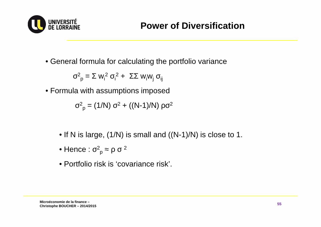
• General formula for calculating the portfolio variance
σ2p = Σ wi
2 σi2 + ΣΣ wiwj σij
• Formula with assumptions imposed
σ2p = (1/N) σ2 + ((N-1)/N) ρσ2
• If N is large, (1/N) is small and ((N-1)/N) is close to 1.
• Hence : σ2p ≈ ρ σ 2
• Portfolio risk is ‘covariance risk’.
Microéconomie de la finance –Christophe BOUCHER – 2014/2015 56
Sta
ndar
d er
ror
No. of shares in portfolio
Diversifiable / idiosyncratic risk
Market / non-diversifiable risk
20 400 1 2 ...
Random selection of stocks
Microéconomie de la finance –Christophe BOUCHER – 2014/2015 57
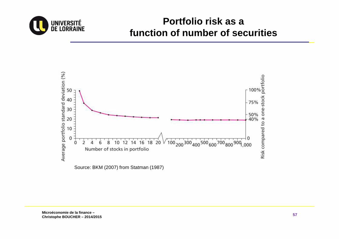
Portfolio risk as a function of number of securities
Source: BKM (2007) from Statman (1987)

Microéconomie de la finance –Christophe BOUCHER – 2014/2015 58
Thank you for your attention…
See you next week