microeconomics -1 - consumers · microeconomics -1 - consumers © john riley october 23, 2018
TRANSCRIPT

Microeconomics -1 - Consumers
© John Riley October 23, 2018
A1. The simple mathematics of elasticity 2
A2. The Envelope Theorem 7
B. Income and substitution effects 15
C. Application: Labor supply 24
D. Determinants of demand 28
E. Measuring consumer gains and losses 38
Technical Notes* 46
1. Equivalent Variation
2. Mathematics of income and substitution effects
3. Superlevel sets of the aggregated utility function
58 slides
*Not examinable. Will be omitted from the lectures.

Microeconomics -2 - Consumers
© John Riley October 23, 2018
A1. Elasticity
Consider the figure opposite. A very useful measure
of the sensitivity of y with respect to z is the
proportional rate of change of y with respect to z .
This is called the “arc elasticity”
Arc elasticity =
y
z yyz y zz
*
Arc elasticity

Microeconomics -3 - Consumers
© John Riley October 23, 2018
A1. Elasticity
Consider the figure opposite. A very useful measure
of the sensitivity of y with respect to z is the
proportional rate of change of y with respect to z .
This is called the “arc elasticity”
Arc elasticity =
y
z yyz y zz
Consider two countries that measure both y
and z in different units.
Y ay and Z bz . Then Y a y and Z b z
It follows that the arc elasticity is the
same.
( ) ( )
( ) ( )
Z Y bz a y z y
Y Z ay b z y z
Arc elasticity

Microeconomics -4 - Consumers
© John Riley October 23, 2018
(Point) Elasticity
In theoretical analysis it is helpful to take the limit
and define the (point) elasticity
Elasticity = ( , ) limz y z dy
y zy z y dz
( )
( )
zf z
f z
*
Point elasticity

Microeconomics -5 - Consumers
© John Riley October 23, 2018
(Point) Elasticity
In theoretical analysis it is helpful to take the limit
and define the (point) elasticity
Elasticity = ( , ) limz y z dy
y zy z y dz
( )
( )
zf z
f z
Note that 1
lnd dy
ydz y dz
. Therefore
( , ) lnz dy d
y z z yy dz dz
.
Using this formula we can derive the following proposition
Elasticity of products and ratios
The elasticity of a product is the sum of the elasticities. ( , ) ( , ) ( , )xy z x z y z
The elasticity of a ratio is the difference in elasticities ( , ) ( , ) ( , )x
z x z y zy
Point elasticity

Microeconomics -6 - Consumers
© John Riley October 23, 2018
Derivation of the sum rule
( , ) lnz dy d
y z z yy dz dz
Consider the elasticity of a product.
( , ) lnd
xy z z xydz
[ln ln ]d
z x ydz
ln lnd d
z x ydz dz
( , ) ( , )x z y z
Group exercises: Group O: Linear demand ,a p
p a bq qb
Group E: Log linear demand , ln ln lnbq ap q a b p

Microeconomics -7 - Consumers
© John Riley October 23, 2018
A2. The Envelope Theorem
Consider the following constrained maximization problem with a parameter p in the function to be
maximized. Let x̂ be the solution when the parameter is p̂ . Let ( )x p be the solution for all p . Let
( )F p be the maximized value.
( ) { ( , ) | ( ) }x
F p Max f x p g x b .
Simple Example: Profit maximization ( ) { ( )}q
F p Max pq C q
To determine the rate at which ( ) ( ( ), )F p f x p p varies with p is appears that it is necessary to first
solve for the maximizer ( )x p and then substitute this into ( , )f x p .
However this intuition is incorrect. The answer is much simpler. On the margin only the direct effect
is a non-zero effect.

Microeconomics -8 - Consumers
© John Riley October 23, 2018
Envelope theorem
0( ) { ( , ) | ( ) }
xF p Max f x p g x b
.
( ( ), )dF f
x p pdp p
Informal proof: Let ˆ ˆ( )x x p be the solution when the price is p̂ .
Suppose that the decision-maker is naïve and does not change output as the parameter changes.
The naïve payoff is ˆ ˆ ˆ( , ) ( ( ), )f x p f x p p .
We compare ( )F p and ˆ( , )f x p .
*

Microeconomics -9 - Consumers
© John Riley October 23, 2018
Envelope theorem
0( ) { ( , ) | ( ) }
xF p Max f x p g x b
.
( ( ), )dF f
x p pdp p
Informal proof: Let ˆ ˆ( )x x p be the solution when the price is p̂ .
Suppose that the decision-maker is naïve and does not change output as the parameter changes.
The naïve payoff is ˆ ˆ ˆ( , ) ( ( ), )f x p f x p p .
Note that
(i) ˆ ˆ ˆ( ) ( ( ), )F p f x p p
Since ( )x p is optimal, for all p
(ii) ˆ( ) ( ( ), ) ( ( ), )F p f x p p f x p p .
Assuming that the functions are differentiable,
the graphs of the two functions must be as
depicted. It follows that the graphs must
be tangential at p̂ . i.e. ˆ( ) ( , )f
F p x pp

Microeconomics -10 - Consumers
© John Riley October 23, 2018
Intuition for the simplest case with no constraint
( ) { ( , )}x
F p Max f x p
There are two effects
1. Direct effect
Parameter change p
ˆ ˆ( , )f x p rises to ˆ( , )f x p p
*

Microeconomics -11 - Consumers
© John Riley October 23, 2018
Intuition for the simplest case with no constraint
( ) { ( , )}x
F p Max f x p
There are two effects
1. Direct effect
Parameter change p
ˆ ˆ( , )f x p rises to ˆ( , )f x p p
2. Indirect effect
Decision variable change x .
For small change in price the
The graph of ( , )f x p has a slope
which is close to zero.
This effect disappears in the limit. Only the direct effect is a “first order effect”.

Microeconomics -12 - Consumers
© John Riley October 23, 2018
A more general result (Not examinable)
( ) { ( , )}x X
F p Max f x p
. Note that x is constrained to belong to some unspecified set.
Proposition: If ( )x p is a continuous function then ( ) ( ( ), )f
F p x p pp
(i) Since 0( )x p is the optimizer when 0p p , it follows that 0 1 00 0 ( ( ), )( ( ), )( ) f x p p f x pF p p .
Therefore 1 0 101 11 00 1 ( ( ), )( ) ( ) ( ( ), ) ( )( ,( (), ) )F p F p f x p p f x pf x p p f xp p p
**

Microeconomics -13 - Consumers
© John Riley October 23, 2018
A more general result (Not examinable)
( ) { ( , )}x X
F p Max f x p
. Note that x is constrained to belong to some unspecified set.
Proposition: If ( )x p is a continuous function then ( ) ( ( ), )f
F p x p pp
.
(i) Since 0( )x p is the optimizer when 0p p , it follows that 0 0 0 1 0( ) ( ( ), ) ( ( ), )F p f x p p f x p p .
Therefore 1 0 1 1 0 0 1 1 1 0( ) ( ) ( ( ), ) ( ( ), ) ( ( ), ) ( ( ), )F p F p f x p p f x p p f x p p f x p p
(ii) Since 1( )x p is the optimizer when 1p p , it follows that 1 0 11 1 ( ( ), )( ( ), )( ) f x p p f x pF p p .
Therefore 01 0 0 11 1 0 0 0( ) ( ) ( ( ), ) ( ( ), )(( ( ), ,) ( ) )f xF p F p f x p p ff x px p p pp p
*

Microeconomics -14 - Consumers
© John Riley October 23, 2018
A more general result (Not examinable)
( ) { ( , )}x X
F p Max f x p
. Note that x is constrained to belong to some unspecified set.
Proposition: If ( )x p is a continuous function then ( ) ( ( ), )f
F p x p pp
.
(i) Since 0( )x p is the optimizer when 0p p , it follows that 0 0 0 1 0( ) ( ( ), ) ( ( ), )F p f x p p f x p p .
Therefore 1 0 1 1 0 0 1 1 1 0( ) ( ) ( ( ), ) ( ( ), ) ( ( ), ) ( ( ), )F p F p f x p p f x p p f x p p f x p p
(ii) Since 1( )x p is the optimizer when 1p p , it follows that 1 1 1 0 1( ) ( ( ), ) ( ( ), )F p f x p p f x p p .
Therefore 1 0 1 1 0 0 0 1 0 0( ) ( ) ( ( ), ) ( ( ), ) ( ( ), ) ( ( ), )F p F p f x p p f x p p f x p p f x p p
Together, these inequalities imply that
0 1 0 0 1 0 1 1 1 0
1 0 1 0 1 0
( ( ), ) ( ( ), ) ( ) ( ) ( ( ), ) ( ( ), )f x p p f x p p F p F p f x p p f x p p
p p p p p p
.
Note that as 1 0p p , the lower and upper bounds both approach 0 0( ( ), )f
x p pp
. Thus the
derivative
0 0 0( ) ( ( ), )f
F p x p pp
. QED

Microeconomics -15 - Consumers
© John Riley October 23, 2018
B. Income and substitution effects on demand
Decomposition of the effects of a price increase
with fixed income
A consumer with income I facing price vector p
chooses x that solves
0
{ ( ) | }x
Max U x p x I
Utility maximization

Microeconomics -16 - Consumers
© John Riley October 23, 2018
B. Income and substitution effects on demand
Decomposition of the effects of a price increase
A consumer with income I , facing price vector p
chooses x that solves
0
{ ( ) | }x
Max U x p x p
The price of commodity 1 rises from 1p to 1p
so the consumer is worse off.
Consider the following thought experiment.
Step 1: Give the consumer enough income compensation
so that she is no worse off, i.e. she ends up on the initial
level set.
Step 2: Take away the compensation
Price increase lowers utility

Microeconomics -17 - Consumers
© John Riley October 23, 2018
Step 1: Compensated demand
The “substitution effect”
Suppose that the consumer is taxed just enough
that her utility is unchanged.
This is called the compensated price effect.
The new optimum is cx .
Since the relative price of commodity 1 has
risen, demand for commodity 1 falls and
demand for commodity 2 rises.
The consumer has substituted away from
the commodity that has become relatively
more expensive.
Compensated effect of the price increase

Microeconomics -18 - Consumers
© John Riley October 23, 2018
Step 2: The compensation is taken away
The “income effect”
A commodity is called “normal” if more of it
Is consumed as income rises.
When the consumer pays back his compensation
Demand for both goods falls if both are normal.
The total effect on demand for commodity 1.
The substitution effect and the income effect
are reinforcing. Both lead to lower demand
for commodity 1.
Income effect

Microeconomics -19 - Consumers
© John Riley October 23, 2018
Income and substitution effects on demand when the consumer has an endowment of
commodities.
Decomposition of the effects of a price increase
A consumer with endowment facing price vector p
chooses x that solves
0
{ ( ) | }x
Max U x p x p
*
Price increase raises utility

Microeconomics -20 - Consumers
© John Riley October 23, 2018
Income and substitution effects on demand
Decomposition of the effects of a price increase
A consumer with endowment facing price vector p
chooses x that solves
0
{ ( ) | }x
Max U x p x p
We consider an increase in the price of commodity 1
As depicted, the consumer’s endowment of
commodity 1 is so high that she is a net seller of
this commodity. Therefore the price increase
raises her utility.
Price increase raises utility

Microeconomics -21 - Consumers
© John Riley October 23, 2018
Substitution effect
Suppose that the consumer is taxed just enough
that her utility is unchanged.
Note that the compensation is now negative.
The new optimum is cx .
Since the relative price of commodity 1 has
risen, demand for commodity 1 falls and
demand for commodity 2 rises.
Compensated effect of the price increase

Microeconomics -22 - Consumers
© John Riley October 23, 2018
Income effect
Now give the tax back to the consumer.
A “normal good” is a commodity for which
consumption rises with income. As depicted
both commodities are normal goods so the
income effect on the consumption of both
commodities is positive.
*
Compensated and income effects

Microeconomics -23 - Consumers
© John Riley October 23, 2018
Income effect
Now give the tax back to the consumer.
A “normal” commodity is a commodity for which
consumption rises with income. As depicted
both commodities are normal goods so the
income effect on the consumption of both
commodities is positive.
Total effect
Thus with normal commodities, the two effects
Are opposing on the commodity for which the
price has increased.
The two effects are reinforcing for the other
commodity.
Compensated and income effects

Microeconomics -24 - Consumers
© John Riley October 23, 2018
C. Application: Labor supply
We now interpret commodity 1
as a consumer’s leisure time. The
price of commodity 1 becomes the wage rate
If he does not work he has 1 units of leisure.
If he supplies 1z units of labor, his income is
1 1p z and so his budget constraint is
2 2 1 1 1p x wz p z . (*)
*
Labor supply
wage
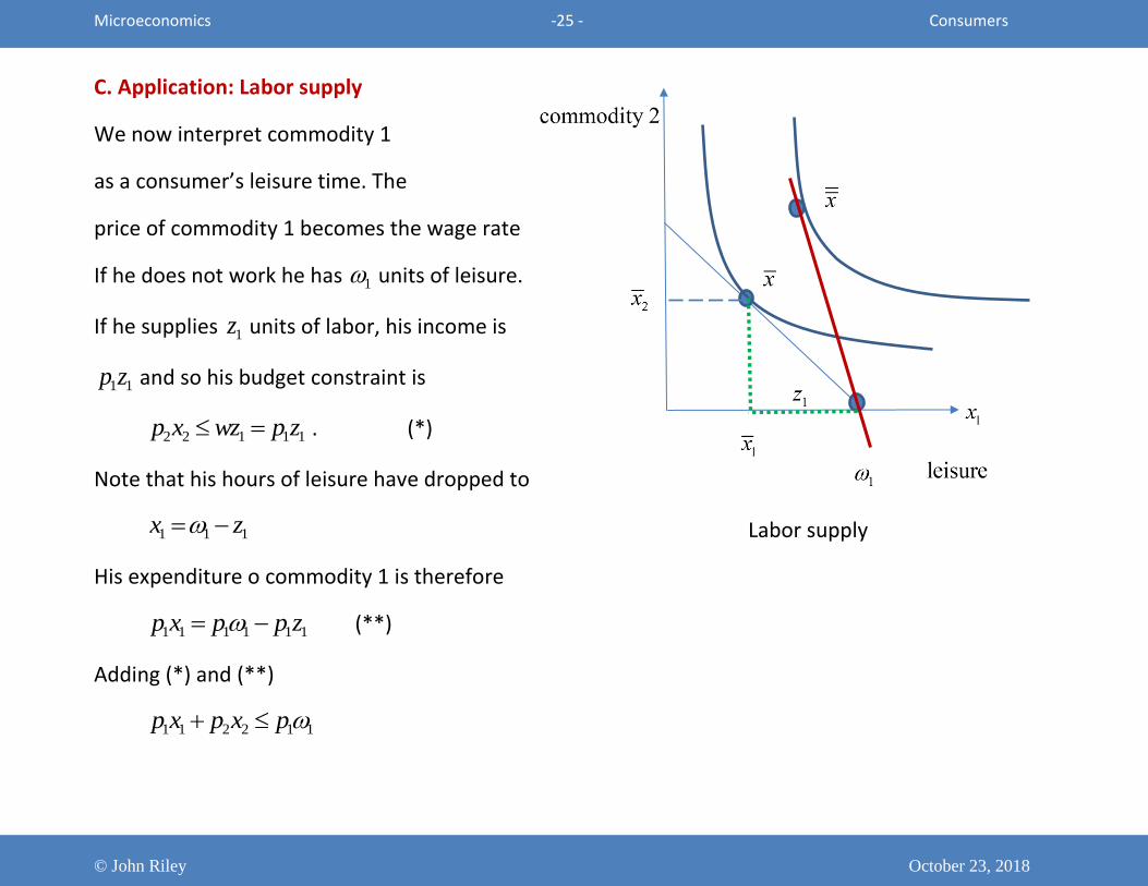
Microeconomics -25 - Consumers
© John Riley October 23, 2018
C. Application: Labor supply
We now interpret commodity 1
as a consumer’s leisure time. The
price of commodity 1 becomes the wage rate
If he does not work he has 1 units of leisure.
If he supplies 1z units of labor, his income is
1 1p z and so his budget constraint is
2 2 1 1 1p x wz p z . (*)
Note that his hours of leisure have dropped to
1 1 1x z
His expenditure o commodity 1 is therefore
1 1 1 1 1 1p x p p z (**)
Adding (*) and (**)
1 1 2 2 1 1p x p x p
Labor supply

Microeconomics -26 - Consumers
© John Riley October 23, 2018
Budget constraint:
1 1 2 2 1 1p x p x p
The value of his consumption of leisure and the
other commodity cannot exceed the value of his
endowment.
**
Compensated effect of the price increase

Microeconomics -27 - Consumers
© John Riley October 23, 2018
Budget constraint:
1 1 2 2 1 1p x p x p
The value of his consumption of leisure and the
other commodity cannot exceed the value of his
endowment.
Substitution effect
The substitution effect of a wage increase (increase in 1p )
is a reduction in demand for commodity 1 and thus an
increase in the labor supply if leisure is a normal commodity.
*
Compensated effect of the price increase

Microeconomics -28 - Consumers
© John Riley October 23, 2018
Budget constraint:
1 1 2 2 1 1p x p x p
The value of his consumption of leisure and the
other commodity cannot exceed the value of his
endowment.
Substitution effect
The substitution effect of a wage increase (increase in 1p )
is a reduction in demand for commodity 1 and thus an
increase in the labor supply if leisure is a normal commodity.
Income effect (normal commodities)
The income effect is to increase demand for leisure
and thus reduce the supply of labor.
Thus the two effects are offsetting.
It is therefore not surprising that data analysis shows that wage effects on the aggregate supply of
labor are small.
Compensated effect of the price increase

Microeconomics -29 - Consumers
© John Riley October 23, 2018
D. Determinants of demand with n commodities
Consider the standard consumer problem
0{ ( ) | }
xMax U x p x I
To better understand the determinants of demand for a commodity (we label it commodity 1) it is
helpful to think of the consumer as solving this problem in two steps.
**

Microeconomics -30 - Consumers
© John Riley October 23, 2018
D. Determinants of demand with n commodities
Consider the standard consumer problem
0{ ( ) | }
xMax U x p x I
where 1 2( , ,..., )nx x x x
To better understand the determinants of demand for a commodity (we label it commodity 1) it is
helpful to think of the consumer as solving this problem in two steps.
Step 1:
Suppose that the consumer must consume 1x units of commodity 1 and is given y to spend on the
other 1n commodities. We write the vector of all the other commodities as 2( ,..., )nz x x and
define the price vector 2( ,..., )nr p p .
Then the consumer solves the following problem.
10
{ ( , ) | }z
Max U x z r z y
.
*

Microeconomics -31 - Consumers
© John Riley October 23, 2018
D. Determinants of demand with n commodities
Consider the standard consumer problem
0{ ( ) | }
xMax U x p x I
where 1 2( , ,..., )nx x x x
To better understand the determinants of demand for a commodity (we label it commodity 1) it is
helpful to think of the consumer as solving this problem in two steps.
Step 1:
Suppose that the consumer must consume 1x units of commodity 1 and is given y to spend on the
other 1n commodities. We write the vector of all the other commodities as 2( ,..., )nz x x and
define the price vector 2( ,..., )nr p p .
Then the consumer solves the following problem.
10
{ ( , ) | }z
Max U x z r z y
.
Let ( )z y be a solution of this maximization problem. Then the maximized utility is
1 1( , ) ( , ( ))u x y U x z y

Microeconomics -32 - Consumers
© John Riley October 23, 2018
Group Exercise:
1/2 1/4 141 2 3( )U x x bx x ,
Budget constraint 1 1 2 2 3 3p x p x p x I .
Step 1:
Fix 1x and allocate y dollars to be spent on 2x and 3x .
So maximize 1/4 142 3bx x (a problem that we have seen a lot)

Microeconomics -33 - Consumers
© John Riley October 23, 2018
Step 2:
Choose 1,x y that solves
1
1 1 1,
{ ( , ) | }x y
Max u x y p x y I .
It is this second step that we now consider.*
*In the figure the superlevel sets of the aggregated utility function are convex. As long as the
superlevel set of ( )U x are strictly convex, then so are the super level sets of 1( , )u x y . If you are
interested in the proof, see the Technical Note at the end.
Aggregated utility function

Microeconomics -34 - Consumers
© John Riley October 23, 2018
1( , )x y solves
1
1 1 1,
{ ( , ) | }x y
Max u x y p x y I .
It is this second step that we now consider.
Decomposition of the effects of a price increase
A consumer with income I facing a price vector p
chooses 1( , )x y that solves
1
1 1,
{ ( , ) | }x y
Max u x y p x y I
We consider an increase in the price of 1x .
In the figure B is the maximizer at the initial
price 1p and B is the maximizer after the price increase.
Price increase raises utility

Microeconomics -35 - Consumers
© John Riley October 23, 2018
Substitution effect
Suppose that the consumer is subsidized just enough
that her utility is unchanged.
This is called the compensated price effect.
The new optimum is the point C .
Since the relative price of commodity 1 has
risen, demand for commodity 1 falls and spending
on other commodities rises .
Compensated price effect

Microeconomics -36 - Consumers
© John Riley October 23, 2018
Income effect (normal goods)
Now give the tax back to the consumer.
A “normal” commodity is a commodity for which
consumption rises with income. As depicted
commodity 1 is a normal commodity so the
income effect is positive, offsetting the
substitution effect.
*
Price increase lowers utility

Microeconomics -37 - Consumers
© John Riley October 23, 2018
Income effect (normal commodity)
Now give the tax back to the consumer.
A “normal good” is a commodity for which
consumption rises with income. As depicted
commodity 1 is a normal commodity so the
income effect is positive, offsetting the
substitution effect.
Theoretical possibility:
Giffen Good: demand increases with price
An example? The price of fuel oil rises sharply in New England. Enough people who were planning to
winter in Florida can no longer afford to do so. They stay home and demand for fuel oil rises.
Price increase lowers utility

Microeconomics -38 - Consumers
© John Riley October 23, 2018
E. Income compensation and consumer surplus
Consider a consumer with income I . At the
initial price 1p her choice is 1( , )x y .
Let ( , )M p u be the income that the consumer
requires to remain on her original indifference
curve as 1p rises. i.e.
1 1 1 10
( , ) { | ( , ) )}x
M p u Min p x y u x y u
.
**
Compensated effect of the price increase

Microeconomics -39 - Consumers
© John Riley October 23, 2018
E. Income compensation and consumer surplus
Consider a consumer with income I . At the
initial price 1p her choice is 1( , )x y .
Let ( , )M p u be the income that the consumer
requires to remain on her original indifference
curve as 1p rises. i.e.
1 1 1 10
( , ) { | ( , ) )}x
M p u Min p x y u x y u
.
1 1 1 10
( , ) { | ( , ) )}x
M p u Max p x y u x y u
*
Compensated effect of the price increase

Microeconomics -40 - Consumers
© John Riley October 23, 2018
E. Income compensation and consumer surplus
Consider a consumer with income I . At the
initial price 1p her choice is 1( , )x y .
Let ( , )M p u be the income that the consumer
requires to remain on her original indifference
curve as 1p rises. i.e.
1 1 1 10
( , ) { | ( , ) )}x
M p u Min p x y u x y u
.
1 1 1 10
( , ) { | ( , ) )}x
M p u Max p x y u x y u
Appealing to the Envelope Theorem
1
1
Mx
p
Then the rate at which this income rises with 1p is
1
1
( , )cMx p u
p
Compensated effect of the price increase

Microeconomics -41 - Consumers
© John Riley October 23, 2018
E. Income compensation and consumer surplus
In the Figure, with the additional income
her consumption choice is C . In the absence of
the compensation her income is I and her
consumption choice is B . Thus to be fully
compensated for the price increase the consumer
must be paid
1( , )M p u I .
Compensated effect of the price increase

Microeconomics -42 - Consumers
© John Riley October 23, 2018
Compensating Variation in income
At the initial price vector no compensation is
necessary so 1( , )M p u I . Then the compensating
income change (called the compensating variation
in income) is
1 1 1( , ) ( , ) ( , )CV M p u I M p u M p u .
*
Compensated demand price function.

Microeconomics -43 - Consumers
© John Riley October 23, 2018
Compensating Variation in income
At the initial price vector no compensation is
necessary so 1( , )M p u I . Then the compensating
income change (called the compensating variation
in income) is
1 1 1( , ) ( , ) ( , )CV M p u I M p u M p u .
Note that the definite integral ( ) ( ) ( )x
x
F x F x F x dx
Therefore
1 1( , ) ( , )CV M p u M p u 1
1
1
1
p
p
Mdp
p
By the Envelope Theorem, 1 1
1
( )cMx p
p
. Therefore
1
1
1 1 1( )p
c
p
CV x p dp
In the figure the compensating variation is the shaded area to the left of the compensated demand
price function.
Compensated demand price function.

Microeconomics -44 - Consumers
© John Riley October 23, 2018
The dotted green ordinary demand function is 1 1( , )x p I
is also depicted. Assuming that commodity 1 is a
normal commodity, income compensation raises
demand when the price rises and lowers demand
when the price falls.
Thus the compensated demand price
function is steeper.

Microeconomics -45 - Consumers
© John Riley October 23, 2018
Estimating the compensating variation
Note that the area to the left of the
compensated demand curve is greater than the area
to the left of the green ordinary
demand price function for a normal good.
However, as Robert Willig showed, for most
such calculations, the difference between
the two areas is small.
In practice economists typically approximate the
compensating variation by measuring the area to the left of the ordinary demand price function.
Remark on the use of survey data

Microeconomics -46 - Consumers
© John Riley October 23, 2018
Technical Notes (not examinable)
1. Equivalent variation in income (EV)
At the new higher price the consumer is worse off.
How much would he be willing to pay to have the initial
price restored?
*

Microeconomics -47 - Consumers
© John Riley October 23, 2018
Equivalent variation in income (EV)
At the new higher price the consumer is worse off.
How much would he be willing to pay to have the initial
price restored?
Arguing as above, he would be willing to pay.
( , )iEV I M p u where ( , )iu u x y
( , ) ( , ))i iM p u M p u
( , ))i i
i i
p p
ci i
p p
Mdp x p u dp
p
This differs from the compensating variation.
However, as noted above, in practice economists
compute the area to the left of the green
“ordinary” demand curve.

Microeconomics -48 - Consumers
© John Riley October 23, 2018
2. The mathematics of substitution and income effects
Definition: The elasticity of substitution for commodity i is the compensated elasticity of the
ratio c
ci
y
x with respect to ip .
( , )i i
i
yp
x
Around the level set as ip increases
c ci
i i i i
x ydu u u
dp x p y p
1
( ) ( ) 0c ci
i
i i i i
x yu up
p x p y p
.
The consumer equates the marginal utility per
dollar. It follows that
0c ci
i
i i
x yp
p p
.
Elasticity of substitution

Microeconomics -49 - Consumers
© John Riley October 23, 2018
In the last slide we showed that
0c ci
i
i i
x yp
p p
We convert this equation into elasticities,
( ) ( ) ( , ) ( , ) 0c c
c ci i ii i i i i
i i i i i
p x p yy yx x x p y p
x p p y p p
.
**

Microeconomics -50 - Consumers
© John Riley October 23, 2018
In the last slide we showed that
0c ci
i
i i
x yp
p p
We convert this equation into elasticities,
( ) ( ) ( , ) ( , ) 0c c
c ci i ii i i i i
i i i i i
p x p yy yx x x p y p
x p p y p p
.
Multiply both terms by ip
I .
( , ) ( , ) 0c ci ii i i
p x yx p y p
I I
*

Microeconomics -51 - Consumers
© John Riley October 23, 2018
In the last slide we showed that
0c ci
i
i i
x yp
p p
We convert this equation into elasticities,
( ) ( ) ( , ) ( , ) 0c c
c ci i ii i i i i
i i i i i
p x p yy yx x x p y p
x p p y p p
.
Multiply both terms by ip
I .
( , ) ( , ) 0c ci ii i i
p x yx p y p
I I
Define the expenditure share i ii
p xk
p x
. Then 1 1 i i
i
p x yk
I I
Therefore
( , ) (1 ) ( , ) 0c ci i i i ik x p k y p

Microeconomics -52 - Consumers
© John Riley October 23, 2018
In the last slide we showed that
( , ) (1 ) ( , ) 0c ci i i i ik x p k y p .
Add (1 ) ( , )ci i ik x p to the first term and subtract it from the second.
Then
( , ) (1 )[ ( , ) ( , )] 0c ci i i i i ix p k y p x p .

Microeconomics -53 - Consumers
© John Riley October 23, 2018
In the last slide we showed that
( , ) (1 ) ( , ) 0c ci i i i ik x p k y p .
Add (1 ) ( , )ci i ik x p to the first term and subtract it from the second.
Then
( , ) (1 )[ ( , ) ( , )] 0c ci i i i i ix p k y p x p .
The term in brackets is the elasticity of substitution, ( , ) ( , ) ( , )c
c ci i i i ic
i
yp y p x p
x .
Therefore
( , ) (1 ) 0ci i i ix p k
Proposition: Price elasticity of compensated demand
The own price elasticity of compensated demand is
( , ) (1 )ci i i ix p k .

Microeconomics -54 - Consumers
© John Riley October 23, 2018
Decomposition of the own price elasticity of demand
Let ( , )i ix p I he the consumer’s uncompensated demand for commodity i . In section E we defined
( , ))iM p u to be the income the consumer would need to maintain a constant utility.
Then the consumer’s compensated demand for commodity i is
( , ( , ))ci i i ix x p M p u .
Differentiating by ip
ci i i
i i i
x x x M
p p I p
.
*

Microeconomics -55 - Consumers
© John Riley October 23, 2018
Decomposition of the own price elasticity of demand
Let ( , )i ix p I he the consumer’s uncompensated demand for commodity i . In section E we defined
( , ))iM p u to be the income the consumer would need to maintain a constant utility.
Then the consumer’s compensated demand for commodity i is
( , ( , ))ci i i ix x p M p u .
Differentiating by ip
ci i i
i i i
x x x M
p p I p
.
Appealing to the Envelope Theorem, i
i
Mx
p
.
We therefore have the following result
Slutsky equation
ci i i
i
i i
x x xx
p p I
.

Microeconomics -56 - Consumers
© John Riley October 23, 2018
Rewrite the Slutsky equation as follows:
c
i i ii
i i
x x xx
p p I
Converting into elasticities,
1ci i i i i
i i
i i i i i
p x p x xp x
x p x p p I
1 1 1 1 1
1 1 1
( )cp x p x xI
x p I p I
.
Therefore
( , ) ( , ) ( , )ci i i i i ix p x p k x I
Appealing to our earlier result, we have the following proposition.
Proposition: Decomposition of the own price elasticity of demand
( , ) ((1 ) ( , ))i i i i i ix p k k x I
The own price elasticity of demand is a convex combination of the elasticity of substitution and the
income elasticity of demand.
Remark: If the fraction spent on commodity 1 is small, then the own price elasticity is approximately
equal to i .

Microeconomics -57 - Consumers
© John Riley October 23, 2018
3. Derived utility function and convex superlevel sets
Proposition: Convexity of the derived utility function
Define 2( ,..., )nr p p and 2( ,..., )nz x x . If ( )U x is strictly increasing and the superlevel sets of ( )U x
are convex then the superlevel sets of
1 1( , ) { ( , ) | }z
u x y Max U x z r z y
are also convex.
Proof:
Suppose that 0 0( , )ix y and 1 1( , )ix y
are, as depicted, in the superlevel set
{( , ) | ( , ) }i iS x y u x y u .
i.e.
0 0( , )iu x y u and 1 1( , )iu x y u (*)
We need to show that for any convex combination,
( , )ix y , ( , )iu x y u .

Microeconomics -58 - Consumers
© John Riley October 23, 2018
From (*)
(i) for some 0z costing 0y , 0 01( , )U x z u and (ii) for some 1z costing 1y , 1 1
1( , )U x z u
Define the convex combinations 0 11 1 1(1 )x x x and 0 1(1 )z z z
By hypothesis the superlevel sets of U are convex so 1( , )U x z u .
It remain to show that z is feasible with income 0 1(1 )y y y .
0z costs 0y so 0(1 )z costs 0(1 )y
1z costs 1y so 1z costs 1y
Then 0 1(1 )z z z costs 0 1(1 )y y y .
So z is feasible.
QED