Micro-abrasion-corrosion maps of

316L stainless steel in artificial saliva A. Hayes, S. Sharifi and M.M. Stack*

Department of Mechanical and Aerospace Engineering, University of Strathclyde,

Glasgow, UK.

*Corresponding author. E-mail address: Margaret.stack@strath.ac.uk

Keywords: 316L stainless steel, artificial saliva, oral cavity, abrasion, corrosion, tribo-corrosion

mechanisms

Abstract

The role of salivary media is essential during mastication and ingestion processes; yet it can hinder the

performance of foreign materials in the oral cavity. The aim of this study was to examine the effects of

applied load and applied electrical potential on the tribo-corrosion mechanisms of 316L stainless steel in

an environment similar to oral cavity conditions. 316L stainless steel is a material commonly used in

dentistry for orthodontic braces, wires and in some cases as dental crowns. This is due to its favourable

corrosion resistance. Relatively few studies have examined the materials performance in an oral

environment. The results of this work were used to generate polarisation curves and wastage and

mechanism maps to describe the material's tribo-corrosion behaviour. A significant difference in

corrosion current densities was observed in the presence of abrasive particles suggesting the removal of

the protective chromium oxide passive film. It was found that the corrosion resistant nature of 316L

stainless steel made its wear mechanism micro-abrasion dominated for all test conditions.

Nomenclature

A

a

b

b0

D

E

F

H

H’

Icorr

Icorr 0

k

Ka

Kao

Surface area of wear scar (m2)

Radius of wear scar (m)

Scar diameter (m)

Pure abrasion scar diameter (m)

Abrasive particle diameter (m)

Applied electrical potential (mV)

Faraday’s constant, 96500 (C mol-1)

Hardness (Pa)

Combined hardness (of surface 1 & 2) (Pa)

Corrosion current density (mA cm-2)

Pure corrosion current density (mA/cm2)

Wear coefficient

Abrasion weight loss (g)

Pure abrasion weight loss (g)

Kac

Kc

Kco

L

M

R

Ra

ρ

S

t

V

v

W

Z

Total weight loss (g)

Corrosion weight loss (g)

Pure corrosion weight loss (g)

Total sliding distance (m)

Atomic mass

Cratering ball radius (m)

Surface roughness (arithmetic average) (µm)

Sample density (kgm-3)

Coefficient of Severity

Experiment duration (sec)

Volume loss (m3)

Volume fraction

Applied load (N)

Number of valence electrons in corrosion

Pag

e2

1. Introduction

The oral cavity represents a significantly challenging environment in materials science. One of

the main existing elements in the oral cavity, which can sometimes be overlooked by the

material scientists, is saliva and its important roles. During the mastication and ingestion

processes, the role of salivary media is multi-faceted i.e. saliva functions as a taste compound

diffuser, a lubricant for oral surfaces, a biochemical agent for food structure and an essential

ingredient for bolus formation and safe ingestion [1]. The surfaces in the oral cavity can

compromise of foreign materials, such as dental replacement and orthodontic materials, which

are constantly surrounded by the salivary media. The interactions between saliva and these

foreign materials can affect the tribo-corrosion performance.

There are various types of advanced ceramics, metals and polymers that have been employed

in modern dentistry, all of which possess many different physical, chemical and aesthetic

properties. 316L stainless steel (AISI classification) is one of the longest serving materials in

dentistry. The corrosion resistance and mechanical properties of 316L stainless steel make it a

desirable option for short to medium term use in the human body. The most common dental

implementation of 316L is in orthodontics where it is used to make wires, brackets and bands

for braces [2]. The low cost and low toxicity of 316L also make it a favourable choice for longer

term implants in developing countries where it is commonly used to make dental crowns.

In recent years, there has been a significant increase in the number of studies examining the

tribo-corrosion properties of materials with medical/dental applications. In some recent

studies, micro-abrasion and corrosion mechanisms of 316L stainless steel in various solutions,

including artificial saliva, have been examined. No studies have however explicitly focused on

the synergistic effects of micro-abrasion and corrosion mechanisms which take place on 316L

stainless steel in an artificial saliva solution [2]–[6].

The purpose of this study is to identify the occurring tribo-corrosion mechanisms where 316L

stainless steel is exposed to an environment which is similar to the oral cavity. This has been

achieved through conducting micro-abrasion-corrosion tests in an artificial saliva solution. The

research results were then analysed and interpreted through tribo-corrosion maps.

2. Experiment Details

2.1 Test Samples

The dimensions of the 316L stainless steel samples were chosen to be 30 mm in length and

breadth, with a thickness of 5 mm to fit the test apparatus platform. The samples were ground

Pag

e3

prior to the tests in order to provide a good quality of surface finish. The flatness was confirmed

by taking Ra measurements using a Surftest SV-2000 (Mitutoyo, Japan). The density of the

samples was confirmed experimentally to be 7.99e6 g/cm3. The chemical composition (Table 1)

of the samples was confirmed using energy dispersive X-ray spectroscopy analysis (EDX).

Table 1 – Chemical composition of 316L stainless steel Table 2 – Chemical composition of artificial saliva [7]

2.2 Test Slurry

The original artificial saliva solution was introduced by Takao Fusayama; however, the

composition of the solution has evolved over the years. The composition used for this study is

reported in Table 2 [7]. It contained electrolytes that can react with metal alloys in a similar

manner to natural saliva and had an approximate pH of 5.5 [6]. Saliva is a complex organic

solution made up of 99% water; the remaining composition is composed of many inorganic ions

(electrolytes), organic compounds (enzymes, antivirals, antibacterials etc.) and proteins which

provide a large range of essential functions. Although saliva has a neutral acidity (pH of 7), due

to the acidity of the modern western diet, saliva usually becomes acidic during mastication (pH

5 to 6). It is not uncommon for proteins, antibacterial agents and enzymes to be added to

artificial organic solutions [8]. Yet these components are unlikely to play a major role in the

micro-abrasion-corrosion mechanisms of stainless steel during mastication. They have

therefore not been included in the solution used in this study.

The artificial saliva solution was mixed with alumina particles (calcined aluminium oxide

powder, Logitech, UK) to form the abrasive slurry. This combination simulates the bolus

formation during mastication. Alumina particles were chosen due to the hardness of the

Element Weight %

Carbon, C 0.03 (max)

Manganese, Mn 2.00 (max)

Phosphorus, P 0.03 (max)

Sulphur, S 0.03 (max)

Silicone, Si 0.75 (max)

Nitrogen, N 0.1 (max)

Chromium, Cr 17 - 20

Nickel, Ni 12 - 14

Molybdenum, Mo 2 - 4

Iron, Fe Bal.

Compound Concentration (gl-1

)

NaCl, Sodium Chloride

0.4

KCl, Potassium Chloride

0.4

CaCl22H2O, Calcium Chloride Dihydrate

0.795

NaH2PO42H2O, Sodium Dihydrogen Phosphate Dihydrate

0.78

Na2S9H2O, Sodium Sulfide Nonahydrate

0.005

CH4N2O, Urea

1

Deionised Water Bal.

Pag

e4

particles. The hardness of the particles can increase the severity of the tests, and high hardness

values have been reported for some foods such as nuts [9], [10]. Previous works examined the

effects of particle size and concentration [11]–[13]. For these tests, a concentration of 30 gl-1 of

particles with the average size of 9 µm was used to maintain the consistency with the previous

studies [3], [6], [14]. The abrasive particles were kept suspended using a mechanical stirrer

during the testing and the solution was replaced after a maximum of one hour testing. Table 3

contains the mechanical properties of the test materials.

Material Test Function Density

(kgm-3

)

Hardness (Vickers)

[GPa]

Young’s Modulus

(GPa)

Fracture

Toughness

(MPa m-1/2

)

AISI 316L

SS

Test Sample 7990 (195) [1.912] 192 100

Alumina Abrasive Particles 3800 (2035) [1.912] 351 3.5 - 6

UHMWPE Cratering Ball

(counter surface)

931 - 935 (541) [5.306] 0.689 3.5

Table 3 – Test material mechanical properties [10], [15], [16]

2.3 Experiment Apparatus

For this testing a TE-66 Micro-Scale Abrasion Tester (Phoenix Tribology, Reading, UK) was used

which operates in accordance with British Standards EN 1071-6: 2007 (Figure 1). This tester

generates round wear scars on the samples using a rotating cratering-ball. The test slurry is fed

over the contact interface between the sample and the cratering-ball using a peristaltic pump

connected to an axel that holds the cratering-ball in place. This axel is driven by a variable

speed DC motor. The test slurry is collected in a solution bath below the contact surface. The

load between the sample and the counter-body was applied using a stack of dead weights.

Here, the load can be finely adjusted using an adjustable counter-weight.

UHMWPE (ultra-high-molecular-weight-polyethylene) balls (K-mac Plastics, Michigan, USA) with

the diameter of 25.4 mm (1 inch) were used for these tests. UHMWPE possesses a very low

friction coefficient and high wear resistance which significantly reduces the interference of the

ball in the wear process [15]. UHMWPE is a non-conductive material and therefore has no

effects on the corrosion currents. The sliding velocity of the tests was kept constant. Three balls

were used during the tests. After each test the balls were measured for deformation, visually

inspected for contamination, cleaned with deionised water. In addition, the balls were

incrementally turned in their fixings after each test to prevent any deformation of the spherical

Pag

e5

shape of the balls. The careful and measured reuse of UHMWPE balls is an economic

compromise that has been adopted in other micro-abrasion studies [6], [17].

Figure 1 – TE-66 Micro-Scale Abrasion Tester

A potentiostat (ACM Instruments, UK) was used to apply electrical potentials to the samples

and measure the corrosion currents. The working electrode (WE) was fixed to the back of the

test samples and the auxiliary (AE) and reference electrodes (RE) were placed in the solution

bath. The test samples were insulated using non-conductive tape with a 1 cm2 square section

left uncovered. It should be noted that these tests were not conducted in a de-aerated

condition.

2.4 Test Methodology

These tests were conducted to examine the effects of applied load and applied electrical

potential on tribo-corrosion mechanisms of 316L stainless steel. As shown in Table 4, the test

matrix consisted of 5 different applied loads and 5 electrical potentials. Several recent studies

have been conducted to examine the particle size and distribution properties of food bolus of

varying hardness [11], [18]. Chen et al and Jalabert-Malbos et al have reported that the forces

Pag

e6

required to break the food into bolus, ranges from 0.06 N for egg whites to 24 N for roasted

peanuts with the majority of common foods requiring less than 5N. Hence, a load range of 0.5

to 4 N has been chosen for the tests.

Also, the highest and the lowest reported intraoral potentials in the literature are -431 and

+300 mV [19]. As a result, the selected range of the electrical potentials for these set of

experiments were from -600 mV to 200 mV to reflect the earlier findings and the condition

changes from cathodic to anodic [6].

The performance of 316L in pure abrasion conditions for each applied load was also

investigated. For this purpose, an applied potential of -960mV was used to provide a cathodic

protection condition for the samples [20]. To study the effects of the presence of the particles

in the solution, cyclic sweep tests were also conducted for each load, with and without

particles, which produced the polarisation curves. The cyclic sweep polarisation tests lasted 30

minutes and applied an electrical potential from -1000mV to 500mV with the sweep rate of

50mVs-1.

The cratering-ball was rotating at the speed of 150 rpm for the duration of 30 minutes. The

combination of the rotational speed and test length resulted in a total sliding distance of 359 m

per test. Previous studies have shown that the average sliding distance per tooth each day is

approximately 1 meter. Thus, each test approximates 1 year of material use as a crown [14].

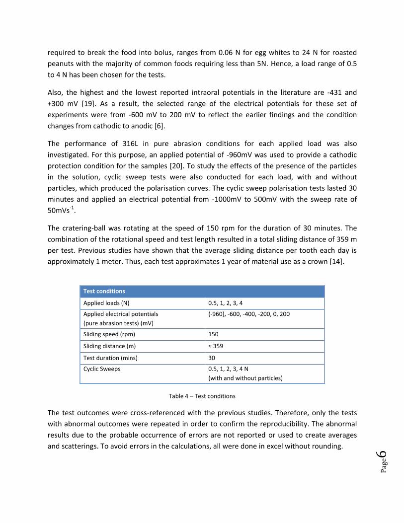
Test conditions

Applied loads (N) 0.5, 1, 2, 3, 4

Applied electrical potentials

(pure abrasion tests) (mV)

(-960), -600, -400, -200, 0, 200

Sliding speed (rpm) 150

Sliding distance (m) ≈ 359

Test duration (mins) 30

Cyclic Sweeps 0.5, 1, 2, 3, 4 N

(with and without particles)

Table 4 – Test conditions

The test outcomes were cross-referenced with the previous studies. Therefore, only the tests

with abnormal outcomes were repeated in order to confirm the reproducibility. The abnormal

results due to the probable occurrence of errors are not reported or used to create averages

and scatterings. To avoid errors in the calculations, all were done in excel without rounding.

Pag

e7

(a)

(b)

3. Results

3.1 Polarisation Curves

Figures 2(a) and 2(b) are the polarisation curves generated from the cyclic sweep tests for all

applied loads, both without and with particles. Figure 2(a) displays more uniformity in corrosion

current densities for all loads in the absence of abrasive particles. This is in comparison with

Figure 2(b) where the abrasive particles are present. It can be seen that the corrosion current

densities for the tests with particles are higher than the tests without particles. With the

exception of 0.5N during cathodic conditions, all the corrosion currents densities are almost ten

times greater with particles than without particles.

Figure 2(a) – Polarisation tests

without particles

Figure 2(b) – Polarisation tests with

particles

Pag

e8

3.2 Alumina particles

In order to have a better understanding of the function of the alumina particles in the tests, a

small amount of the fresh particles was compared with the used particles collected from the

solution bath. The images were taken using a S3700 (Hitachi, Japan) Tungsten Filament

Scanning Electron Microscope (SEM). As shown in Figure 3, the size of the particles did not

seem to be altered after the test. This confirmed the validity of the particles material selection

to avoid degradation. If the hardness of the abrasive particles and the target surface are

relatively close, the wear rate can vary due to the occurrence of a phenomenon known as ‘soft

abrasion’. This takes place when the hardness of the abrasive particles alters during the

interaction [21]. It should be noted that the size values in the two images are there to facilitate

the comparison.

Figure 3 – Particle distribution (a) before and (b) after testing

Figure 4 – Particle embedment on the cratering ball surface after testing (a) SEM image (b) EDX analysis

(a) (b)

Al

(a) (b)

Pag

e9

The cratering ball was also inspected, after a test and before cleaning, for the occurrence of

particle embedment on the ball surface. As depicted in Figure 4, the embedment was observed

on the surface and this was confirmed using EDX analysis. The embedment of particles on the

cratering surface increases the tendency of transition of the abrasion mechanism from 3-body

rolling towards 2-body-grooving [22].

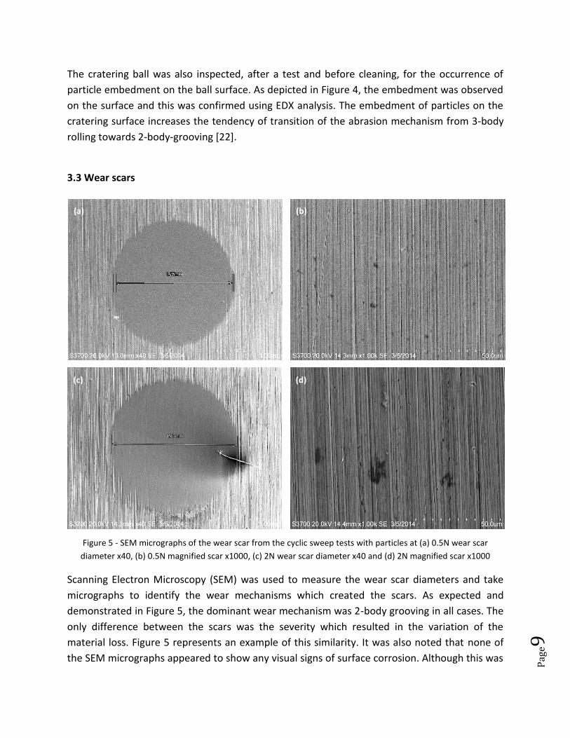
3.3 Wear scars

Figure 5 - SEM micrographs of the wear scar from the cyclic sweep tests with particles at (a) 0.5N wear scar

diameter x40, (b) 0.5N magnified scar x1000, (c) 2N wear scar diameter x40 and (d) 2N magnified scar x1000

Scanning Electron Microscopy (SEM) was used to measure the wear scar diameters and take

micrographs to identify the wear mechanisms which created the scars. As expected and

demonstrated in Figure 5, the dominant wear mechanism was 2-body grooving in all cases. The

only difference between the scars was the severity which resulted in the variation of the

material loss. Figure 5 represents an example of this similarity. It was also noted that none of

the SEM micrographs appeared to show any visual signs of surface corrosion. Although this was

(a) (b)

(c) (d)

Pag

e10

consistent with the previous studies findings [3], [6], after completing the SEM, a number of

samples were cut through the scars and mounted to investigate the cross-section of the scars.

This provided an opportunity for the inspection of the cross-sectional shape of the scars,

existence of corroded layers on the. Figure 6 exhibits the images that were taken from the scars

cross-sections using an optical microscope (Olympus GX51, Japan). Figure 6(a) confirms the

hemispherical shape of the scars. By increasing the magnification and focusing in the middle

area of the scars, it was still not possible to identify any clear corrosion layers. This can be due

to the lower mass of corrosion wear recorded comparing to the mechanical wear. This is

discussed in detail in the next section. From the microscopy results, it was also noted that the

substrate material did not exhibit any form of uninform corrosion or pitting. Figure 6(c) shows

the difference between the sample surface and the scar surface and Figure 6(d) is a cross-

section of the grooves on a scar surface.

Figure 6 – Optical microscopy images from the scars cross-sections (a) 0.5N -600mV - full scar, (b) 2N cyclic sweep

test with particles- full scar, (c) 2N -400mV - scar edge and (d) 0.5N -600mV middle area

(a) (b)

(c) (d)

Wear scar

Pag

e11

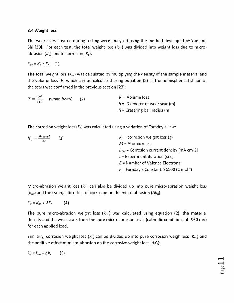
3.4 Weight loss

The wear scars created during testing were analysed using the method developed by Yue and

Shi [20]. For each test, the total weight loss (Kac) was divided into weight loss due to micro-

abrasion (Ka) and to corrosion (Kc).

Kac = Ka + Kc (1)

The total weight loss (Kac) was calculated by multiplying the density of the sample material and

the volume loss (V) which can be calculated using equation (2) as the hemispherical shape of

the scars was confirmed in the previous section [23]:

𝑉 =𝜋𝑏4

64𝑅 (when b<<R) (2) V = Volume loss

b = Diameter of wear scar (m)

R = Cratering ball radius (m)

The corrosion weight loss (Kc) was calculated using a variation of Faraday’s Law:

𝐾𝑐 =𝑀𝐼𝑐𝑜𝑟𝑟𝑡

𝑍𝐹 (3) Kc = corrosion weight loss (g)

M = Atomic mass

Icorr = Corrosion current density [mA cm-2]

t = Experiment duration (sec)

Z = Number of Valence Electrons

F = Faraday’s Constant, 96500 (C mol-1)

Micro-abrasion weight loss (Ka) can also be divided up into pure micro-abrasion weight loss

(Kao) and the synergistic effect of corrosion on the micro-abrasion (∆Ka):

Ka = Kao + ∆Ka (4)

The pure micro-abrasion weight loss (Kao) was calculated using equation (2), the material

density and the wear scars from the pure micro-abrasion tests (cathodic conditions at -960 mV)

for each applied load.

Similarly, corrosion weight loss (Kc) can be divided up into pure corrosion weigh loss (Kco) and

the additive effect of micro-abrasion on the corrosive weight loss (∆Kc):

Kc = Kco + ∆Kc (5)

Pag

e12

Approximate values of pure-corrosion weight loss (Kco) were calculated using equation (3) and

the ‘Icorr’ values from the polarisation curves without particles (Icorr0) for every applied load and

each electrical potential.

(a) (b)

(c) (d)

(e)

Figure 7 – Weight loss graphs of 316L stainless steel for

the load range of 0.5 - 4 N at (a) -600 mV, (b) -400 mV,

(c) -200 mV, (d) 0 mV, and (e) +200 mV.

Pag

e13

Figure 7 presents the calculated total weight loss (Kac), the micro-abrasion weight loss (Ka) (LHS

axes), and the corrosion weight loss (Kc) (RHS axis) results. It should be noted that the scales of

the LHS axes are much higher than the RHS ones. The results show that for every test condition

the total and micro-abrasion weight loss values are very close in magnitude, whilst the

corrosion weight loss is much less. There is also very little variation in total/micro-abrasion

weight loss for each load over a range of applied potentials. For each applied load the corrosion

weight loss increases with increasing applied potential. There is only a very small increase in

abrasion weight loss when corrosion is included (Kao >> ∆Ka). Yet the corrosion is roughly ten

times greater when abrasion is included (Kc ≈ 10Kco).

4. Discussion

The ability to predict wear of materials is a universal challenge crucial to successful application

of new materials into different technologies. There are numerous methods to describe wear

data such as tabulated wear rates or elucidation of the dominant wear mechanisms using

micro-graphs [24]. Of all these methods, a more comprehensive method is to link the wear

rates and wear mechanisms in a much wider range of sliding conditions known as ‘wear maps’.

There are a limited number of standardised wear testing methods and often the variables of a

study are incomparable with one another. Hence, wear (mechanism) maps can be an extra-

ordinary informative tool to link mechanisms to operating parameters [25].

4.1 Tribo-corrosion maps

Wastage and mechanism maps were generated for 316L stainless steel using the test results

(with particles) and mapping techniques have been developed in previous studies [26], [27].

The maps were drawn by plotting the results of the 25 tests on a chart and interpolating

between the points to determine the boundary lines. It had to be assumed that the wear

results varied linearly between each condition.

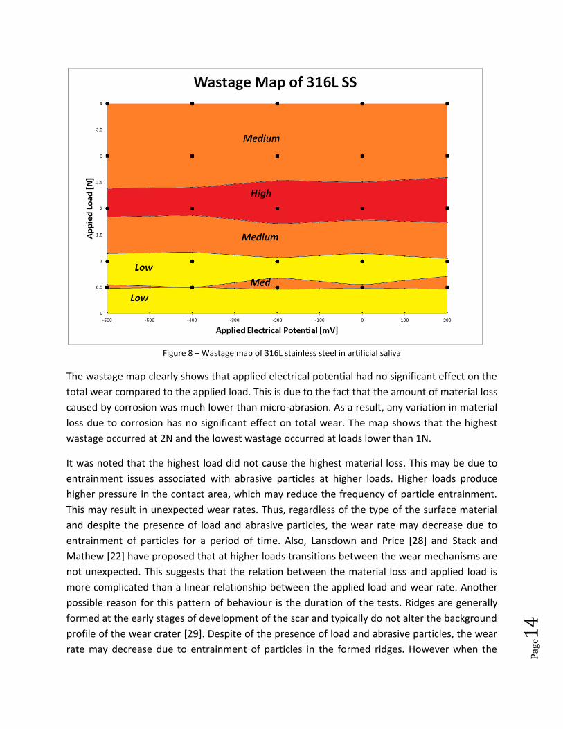
For the wastage map (Figure 8) the categories of wear were taken from previous studies [3],

[6], [14], [20] and adapted as follows:

Very Low: Kac ≤ 0.15 * Kac max

Low: 0.15 * Kac max < Kac ≤ 0.35 * Kac max

Medium: 0.35 * Kac max < Kac ≤ 0.80 * Kac max

High: 0.80 * Kac max < Kac

Pag

e14

Figure 8 – Wastage map of 316L stainless steel in artificial saliva

The wastage map clearly shows that applied electrical potential had no significant effect on the

total wear compared to the applied load. This is due to the fact that the amount of material loss

caused by corrosion was much lower than micro-abrasion. As a result, any variation in material

loss due to corrosion has no significant effect on total wear. The map shows that the highest

wastage occurred at 2N and the lowest wastage occurred at loads lower than 1N.

It was noted that the highest load did not cause the highest material loss. This may be due to

entrainment issues associated with abrasive particles at higher loads. Higher loads produce

higher pressure in the contact area, which may reduce the frequency of particle entrainment.

This may result in unexpected wear rates. Thus, regardless of the type of the surface material

and despite the presence of load and abrasive particles, the wear rate may decrease due to

entrainment of particles for a period of time. Also, Lansdown and Price [28] and Stack and

Mathew [22] have proposed that at higher loads transitions between the wear mechanisms are

not unexpected. This suggests that the relation between the material loss and applied load is

more complicated than a linear relationship between the applied load and wear rate. Another

possible reason for this pattern of behaviour is the duration of the tests. Ridges are generally

formed at the early stages of development of the scar and typically do not alter the background

profile of the wear crater [29]. Despite of the presence of load and abrasive particles, the wear

rate may decrease due to entrainment of particles in the formed ridges. However when the

Pag

e15

ridge is eventually removed, a sudden increase is observed in the wear rate. Previous work by

the current authors [6] for a similar load range showed the highest wear rate was found to be

at 4N load, but this was after 3 hours of testing.

For the mechanism map (Figure 9) the categories of the mechanisms were adopted from the

previous work of the group [20]. An additional ‘pure micro-abrasion’ category was added since

the map was micro-abrasion dominated. The categories were as follows:

Pure micro-abrasion: Kc/Ka ≤ 0

Micro-abrasion: 0 < Kc/Ka < 0.1

Micro-abrasion–corrosion: 0.1 ≤ Kc/Ka < 1

Corrosion–micro-abrasion: 1 ≤ Kc/Ka < 10

Corrosion: 10 ≤ Kc/Ka

Figure 9 – Mechanism map of 316L stainless steel in artificial saliva

The mechanism map of 316L SS stainless steel shows that the wear mechanism is heavily micro-

abrasion dominated. For example, from the results showed that at the highest ratio of

corrosion to micro abrasion (0.5N at 200mV), micro-abrasion is still thirty times greater than

the corrosion. The mechanism map also highlights that under pure micro-abrasion (cathodic),

the highest electrical potential was observed for 2N load and at the lowest for 0.5 and 1N. The

Pag

e16

Pourbaix Diagrams for iron and chromium [30] indicated that the corrosion of iron begins at a

higher electrical potential than chromium. This suggests that more of the chromium oxide

passive film has been removed for loads of 2N compared to 0.5 and 1N. This is consistent with

the results displayed in the wastage map that display the highest wastage at 2N and the lowest

wastage at load bellow 1N.

4.2 Corrosion and Passive Film Removal

For all applied loads, the corrosion current densities were greater for the cyclic sweeps

(polarisation curves) with the presence of abrasive particles than that in their absence (Figure

2). This is an indication that the chromium oxide passive film, which protects the iron from

oxidising, had been removed by the abrasion of the alumina particles. This could mean that the

corrosion in tests without particles is largely from the chromium reacting with the chloride in

the saliva solution, whilst the corrosion in tests with particles is mostly from iron oxidation on

the samples’ un-protected surface [31].

This can be confirmed by the electrical potential at which passivation occurs and by the

presence of repassivation phenomenon observed in the polarisation curves for 2, 3 and 4N with

particles (Figure 2(b)). According to the Pourbaix diagram for chromium [30], pure chromium

will not passivate in a chloride solution with a pH of 5.5, but in other solutions chromium will

passivate at potentials above -500 mV. Since the artificial saliva solution contains a low chloride

concentration and non-chloride electrolytes, it can be assumed that the passivation at

approximately -500mV in all polarisation curves (Figures 2 (a) and (b)) is a result of the

corrosion of the chromium oxide passive film. For iron, the Pourbaix diagram for iron indicates

passivation in a solution of pH of 5.5 at applied electrical potentials greater than 300mV. This is

a likely explanation for the repassivation phenomena observed in the polarisation curves for 2,

3 and 4N with particles.

The weight loss results (Figure 3) indicate a relationship between the rate of micro-abrasion

and corrosion. For applied electrical potentials greater than -200mV (anodic) the rate of

corrosion increases when the rate of micro-abrasion increases;conversely the rate of corrosion

decreases when the rate of micro-abrasion decreases (Figure 10). This would appear to suggest,

that for anodic conditions, when the rate of micro-abrasion increases, the rate at which the

chromium oxide passive film is removed also increases resulting in more iron oxidation. If this is

correct then there should also be a relationship between the rate of micro-abrasion and

presence of repassivation phenomena. Repassivation phenomena can be observed in the

polarisation curves of 2, 3 and 4N which are the three loads with the highest micro-abrasion.

The loads resulting in the lowest micro-abrasion, 0.5 and 1N, display no repassivation. 2N is the

Pag

e17

load with the highest micro-abrasion and it has a greater frequency of repassivation. Of the

loads displaying repassivation, 3N has the lowest micro-abrasion and this also has the lowest

frequency of repassivation. This suggests that higher rates of micro-abrasion also remove the

repassivation film at a higher rate.

Figure 10 – Graph of corrosion of 316L

stainless steel

Figure 11 – Mean total wear for all loads

with standard error for all applied

electrical potentials

4.3 Total Wear

The non-linear relationship between applied load and micro-abrasion observed in this study’s

results is consistent with a previous study of 316L stainless steel in artificial saliva [6]. Other

recent studies of different materials and solutions suggest that applied electrical potential has

no observable effect on the rate of micro-abrasion [20]. This conclusion appears to be

consistent with the results of this study since the total wear of each applied load is constant for

all applied electrical potentials. This can be further confirmed by the graph above (Figure 11)

Pag

e18

which displays the mean total micro-abrasion mass change for each applied load with a

standard error showing the wear variation over all applied electrical potentials. The ‘error’

shows a very low variation between the 5 applied electrical potentials. A standard error for

every electrical potential cannot be generated because only abnormal (unreportable) test

results were repeated.

4.4 Wear Severity Coefficients

In recent literature two different methods have been used to express the severity of total wear.

The first is based on the work of J. F. Archard who established an equation to predict the

volume loss of a material [32]:

𝑉 =𝐾𝑊𝐿

𝐻 (6)

Where ‘V’ is the predicted volume loss, ‘K’ is a constant dimensionless coefficient of wear, ‘W’

is the applied load, ‘L’ is the total sliding distance and ‘H’ is the hardness of the softer of the

two surfaces (in Vickers). If the measured volume loss is used for ‘V’, then ‘K’ can be calculated

for each test condition. Archard’s prediction assumes that total wear will increase linearly as

load and sliding distance increases. This is has been proven true for adhesive sliding wear and

to some extent for hard particle abrasive wear [33], [34]. For non-linear wear ‘K’ can then be

classed as a measure of severity (Figure 12).

Figure 12 – Archard’s coefficient of

wear for 316L stainless steel

The results for Archard’s wear coefficients show that the coefficients are constant for all

applied electrical potentials for each applied load. The results also show a decreasing severity

with increasing applied load with the highest severity occurring at 0.5N and the lowest at 4N.

Pag

e19

This is likely due to the fact that Archard’s prediction assumes that the greatest wear will be

observed at higher loads.

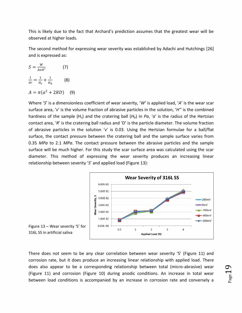
The second method for expressing wear severity was established by Adachi and Hutchings [26]

and is expressed as:

𝑆 =𝑊

𝐴𝑣𝐻′ (7)

1

𝐻′=

1

𝐻𝑠+

1

𝐻𝑏 (8)

𝐴 = 𝜋(𝑎2 + 2𝑅𝐷) (9)

Where ‘S’ is a dimensionless coefficient of wear severity, ‘W’ is applied load, ‘A’ is the wear scar

surface area, ‘v’ is the volume fraction of abrasive particles in the solution, ‘H’’ is the combined

hardness of the sample (Hs) and the cratering ball (Hb) in Pa, ‘a’ is the radius of the Hertzian

contact area, ‘R’ is the cratering ball radius and ‘D’ is the particle diameter. The volume fraction

of abrasive particles in the solution ‘v’ is 0.03. Using the Hertzian formulae for a ball/flat

surface, the contact pressure between the cratering ball and the sample surface varies from

0.35 MPa to 2.1 MPa. The contact pressure between the abrasive particles and the sample

surface will be much higher. For this study the scar surface area was calculated using the scar

diameter. This method of expressing the wear severity produces an increasing linear

relationship between severity ‘S’ and applied load (Figure 13):

Figure 13 – Wear severity ‘S’ for

316L SS in artificial saliva

There does not seem to be any clear correlation between wear severity ‘S’ (Figure 11) and

corrosion rate, but it does produce an increasing linear relationship with applied load. There

does also appear to be a corresponding relationship between total (micro-abrasive) wear

(Figure 11) and corrosion (Figure 10) during anodic conditions. An increase in total wear

between load conditions is accompanied by an increase in corrosion rate and conversely a

Pag

e20

decrease in total wear is accompanied by a decrease in corrosion rate. Also, by comparing the

two methods of evaluating the wear rate (Figures 12 and 13), an existing correlation can be

suggested between the Archard wear coefficient and inverse of wear severity:

𝐾 ∝1

𝑆 (10).

4.5 Wear Regimes

As mentioned earlier, the non-linear relationship between applied load and micro-abrasion is

largely due to the transitions between different wear regimes. The two simplified classifications

of hard particle abrasive wear regimes are two and three-body abrasive wear [21]. More recent

studies in abrasion wear regime transitions have established that there are more regimes

including mixtures of these wear regimes but the fundamental concepts and classifications of

these two modes still hold [17], [22]. It was originally thought that three-body rolling wear

occurs at lower loads and this transitions to two-body grooving at higher loads [21]. More

recent studies have established that as applied load is increased the wear regime transitions

from a mixture of three and two body wear to two body wear and then back to a mixture of

three and two body wear [22], [35].

In addition to establishing the calculation for wear severity ‘S’, Adachi and Hutchings [26] were

also able to quantify the wear severity at which regime transitions occur for a given surface to

cratering ball hardness ratio. Based on multiple micro-abrasion test studies of different

materials using various abrasive particles and solutions, they proposed that three-body abrasive

wear will transition to two-body abrasive wear when:

𝑆 =𝑊

𝐴𝑣𝐻′ > 𝛼 (𝐻𝑠

𝐻𝑏)

𝛽

(10)

Dimensionless constants: α = 0.0076 β = -0.49

where the notation is the same as for the severity of wear ‘S’ (Equations 7-9). The surface to

cratering ball hardness ratio for 316L SS and UHMWPE is 0.36 (see Table 3). This means, that

according to Adachi and Hutchings’ prediction, the wear regime is expected to transition from

three to two-body wear at a wear severity value of 0.01254. The mean wear severity values for

each applied load and the transition conditions are plotted in the Figure 14. According to this

prediction three-body wear should be present at 0.5N, two-body wear at loads of 1N and

higher and the possibility of a mixed wear regime at 0.5, 1 and 2N. Some of these wear regimes

can be confirmed by the SEM micrographs of the wear scars (Figure 15).

Pag

e21

Figure 14 - Predicted wear regimes for 316L SS at different loads

(a) (b) (c)

Figure 15 – SEM micrographs of

wear scars from the cyclic sweep

tests (x1000 magnification) for (a)

0.5N, (b) 1N, (c) 2N, (d) 3N and (e)

4N.

(d) (e)

Two-Body Wear

Three-Body Wear

Pag

e22

The SEM micrographs for 0.5N samples show signs of non-directional wear suggesting three-

body rolling wear (Figure 5(a)). If the magnification of the 0.5N micrographs is increased, the

signs of directional wear can be observed (Figure 15(a)). This is potentially caused by two-body

grooving wear indicating a mixed wear regime at 0.5N. The SEM micrographs for 1N samples

show a slight increase in two-body grooving wear, but it appeared to still be displaying a mixed

regime (Figure 15(b)). For samples of 2N and higher very clear two-body grooving can be

observed suggesting that by 2N the wear regime has fully transitioned to two-body wear

(Figures 15(c) to (e)). These micrograph results appear to be consistent with the Adachi and

Hutchings prediction for wear regime transition.

5. Conclusions

A study of the effects of applied load and electrical potential on the micro-abrasion-

corrosion mechanisms of 316L stainless steel in artificial saliva has been carried out.

The results from the micro-abrasion-corrosion tests were used to generate polarisation

curves, wastage and mechanism maps and to describe the material’s tribo-corrosion

behaviour in a simulated oral environment.

It was found that the corrosion resistant nature of 316L stainless steel made its wear

mechanism micro-abrasion dominated for all test conditions.

The superior corrosion resistance of 316L stainless steel has resulted in a micro-abrasion

rate to be significantly higher than corrosion rate. This was confirmed by the microscopy

inspection as any visual signs of surface corrosion had been removed by the micro-

abrasion mechanisms which predominate.

The polarisation curve results displayed a significant increase in corrosion current

density in the presence of abrasive particles suggesting the removal of the protective

chromium oxide passive film.

The micro-abrasion and corrosion weight loss results suggest that the rate of corrosion

in anodic conditions increases with the increase of micro-abrasion.

Repassivation phenomena were observed in the polarisation curves with higher micro-

abrasion. A higher frequency of repassivation was observed for higher rates of micro-

abrasion.

Pag

e23

References

[1] J. Chen, “Food oral processing: Some important underpinning principles of eating and sensory perception,” Food Struct., vol. 1, no. 2, pp. 91–105, Apr. 2014.

[2] M. Mirjalili, M. Momeni, N. Ebrahimi, and M. H. Moayed, “Comparative study on corrosion behaviour of Nitinol and stainless steel orthodontic wires in simulated saliva solution in presence of fluoride ions.,” Mater. Sci. Eng. C. Mater. Biol. Appl., vol. 33, no. 4, pp. 2084–93, May 2013.

[3] C. Hodge and M. M. Stack, “Tribo-corrosion mechanisms of stainless steel in soft drinks,” Wear, vol. 270, no. 1, pp. 104–114, 2010.

[4] A. Kocijan, D. K. Merl, and M. Jenko, “The corrosion behaviour of austenitic and duplex stainless steels in artificial saliva with the addition of fluoride,” Corros. Sci., vol. 53, no. 2, pp. 776–783, Feb. 2011.

[5] R. A. Antunes, A. C. D. Rodas, N. B. Lima, O. Z. Higa, and I. Costa, “Study of the corrosion resistance and in vitro biocompatibility of PVD TiCN-coated AISI 316L austenitic stainless steel for orthopedic applications,” Surf. Coatings Technol., vol. 205, no. 7, pp. 2074–2081, Dec. 2010.

[6] D. Holmes, S. Sharifi, and M. M. Stack, “Tribo-corrosion of steel in artificial saliva,” Tribol. Int., vol. 75, pp. 80–86, Jul. 2014.

[7] J. Z. Shen, A. Tampieri, J. Chevalier, H. Engqvist, J. Ferreira, E. Sánchez Vilches, P. Bowen, A. Krell, Z. Zhe, L. Wang, Y. Liu, W. Si, H. Feng, Y. Tao, and Z. Ma, “Friction and wear behaviors of dental ceramics against natural tooth enamel,” J. Eur. Ceram. Soc., vol. 32, no. 11, pp. 2599–2606, 2012.

[8] D. Sun, J. A. Wharton, and R. J. K. Wood, “Micro-abrasion mechanisms of cast CoCrMo in simulated body fluids,” Wear, vol. 267, no. 11, pp. 1845–1855, Oct. 2009.

[9] H. Gocmez, M. Tuncer, I. Uzulmez, and O. Sahin, “Particle formation and agglomeration of an alumina–zirconia powder synthesized an supercritical CO2 method,” Ceram. Int., vol. 38, no. 2, pp. 1215–1219, 2012.

[10] V. Muthukumaran, V. Selladurai, S. Nandhakumar, and M. Senthilkumar, “Experimental investigation on corrosion and hardness of ion implanted AISI 316L stainless steel,” Mater. Des., vol. 31, no. 6, pp. 2813–2817, 2010.

[11] J. Chen, N. Khandelwal, Z. Liu, and T. Funami, “Influences of food hardness on the particle size distribution of food boluses,” Arch. Oral Biol., vol. 58, no. 3, pp. 293–298, 2013.

[12] C. G. Telfer, M. M. Stack, and B. D. Jana, “Particle concentration and size effects on the erosion-corrosion of pure metals in aqueous slurries,” Tribol. Int., vol. 53, pp. 35–44, 2012.

[13] M. M. Stack, W. Huang, G. Wang, and C. Hodge, “Some views on the construction of bio-tribo-corrosion maps for Titanium alloys in Hank’s solution: Particle concentration and applied loads effects,” Tribol. Int., vol. 44, no. 12, pp. 1827–1837, 2011.

[14] S. Sharifi and M. M. Stack, “A comparison of the tribological behaviour of Y-TZP in tea and coffee under micro-abrasion conditions,” J. Phys. D. Appl. Phys., vol. 46, no. 40, p. 404008, Oct. 2013.

[15] K. Marcus and C. Allen, “The sliding wear of ultrahigh molecular weight polyethylene in an aqueous environment,” Wear, vol. 178, no. 1–2, pp. 17–28, Nov. 1994.

Pag

e24

[16] J. Y. Wong and J. D. Bronzino, Biomaterials. CRC Press, 2007, p. 296.

[17] R. I. Trezona, D. N. Allsopp, and I. M. Hutchings, “Transitions between two-body and three-body abrasive wear: influence of test conditions in the microscale abrasive wear test,” Wear, vol. 225–229, no. null, pp. 205–214, Apr. 1999.

[18] M.-L. Jalabert-Malbos, A. Mishellany-Dutour, A. Woda, and M.-A. Peyron, “Particle size distribution in the food bolus after mastication of natural foods,” Food Qual. Prefer., vol. 18, no. 5, pp. 803–812, 2007.

[19] Y. Oshida, Bioscience and Bioengineering of Titanium Materials. Elsevier, 2013, pp. 35–85.

[20] M. M. Stack, J. Rodling, M. T. Mathew, H. Jawan, W. Huang, G. Park, and C. Hodge, “Micro-abrasion–corrosion of a Co–Cr/UHMWPE couple in Ringer’s solution: An approach to construction of mechanism and synergism maps for application to bio-implants,” Wear, vol. 269, no. 5, pp. 376–382, 2010.

[21] I. Hutchings, Tribology, Friction and Wear of Engineering Materials. Elsevier Limited, 1992, p. 284.

[22] M. . Stack and M. Mathew, “Micro-abrasion transitions of metallic materials,” Wear, vol. 255, no. 1–6, pp. 14–22, Aug. 2003.

[23] M. G. Gee, A. Gant, I. Hutchings, R. Bethke, K. Schiffman, K. Van Acker, S. Poulat, Y. Gachon, and J. von Stebut, “Progress towards standardisation of ball cratering,” Wear, vol. 255, no. 1, pp. 1–13, 2003.

[24] S. . Lim, “Recent developments in wear-mechanism maps,” Tribol. Int., vol. 31, no. 1, pp. 87–97, 1998.

[25] S. Amini and A. Miserez, “Wear and abrasion resistance selection maps of biological materials,” Acta Biomater., vol. 9, no. 8, pp. 7895–7907, 2013.

[26] K. Adachi and I. M. Hutchings, “Wear-mode mapping for the micro-scale abrasion test,” Wear, vol. 255, no. 1, pp. 23–29, 2003.

[27] M. M. Stack, N. Corlett, and S. Zhou, “A methodology for the construction of the erosion-corrosion map in aqueous environments,” Wear, vol. 203–204, pp. 474–488, Mar. 1997.

[28] A. R. Lansdown and A. L. Price, Materials to Resist Wear (Materials Engineering Practice). Pergamon, 1986, p. 200.

[29] P. . Shipway and C. J. . Hodge, “Microabrasion of glass – the critical role of ridge formation,” Wear, vol. 237, no. 1, pp. 90–97, 2000.

[30] M. Pourbaix, Atlas of electrochemical equilibria in aqueous solutions. National Association of Corrosion Engineers, 1974, p. 644.

[31] S. L. Johnson, “Surface studies of potentially corrosion resistant thin film coatings on chromium and type 316L stainless steel,” Kansas State University, 2006.

[32] J. F. Archard, “Contact and Rubbing of Flat Surfaces,” J. Appl. Phys., vol. 24, no. 8, p. 981, Aug. 1953.

[33] B. Bera, “Adhesive Wear Theory of Micromechanical Surface Contact,” Int. J. Comput. Eng. Res., vol. 3, no. 3, pp. 73–78, 2013.

[34] R. V. Camerini, R. B. de Souza, F. de Carli, A. S. Pereira, and N. M. Balzaretti, “Ball cratering test on ductile materials,” Wear, vol. 271, no. 5, pp. 770–774, 2011.

Pag

e25

[35] R. . Trezona and I. . Hutchings, “Three-body abrasive wear testing of soft materials,” Wear, vol. 233, pp. 209–221, 1999.