micomechanical modeling of porous shape memory alloys

MICROMECHANICAL MODELING OF

POROUS SHAPE MEMORY ALLOYS

A Dissertation

by

PAVLIN BORISSOV ENTCHEV

Submitted to the Office of Graduate Studies ofTexas A&M University

in partial fulfillment of the requirements for the degree of

DOCTOR OF PHILOSOPHY

May 2002

Major Subject: Aerospace Engineering

MICROMECHANICAL MODELING OF

POROUS SHAPE MEMORY ALLOYS

A Dissertation

by

PAVLIN BORISSOV ENTCHEV

Submitted to Texas A&M Universityin partial fulfillment of the requirements

for the degree of

DOCTOR OF PHILOSOPHY

Approved as to style and content by:

Dimitris C. Lagoudas(Chair of Committee)

John. C. Slattery(Member)

Jay R. Walton(Member)

Junuthula N. Reddy(Member)

Ramesh Talreja(Head of Department)

May 2002

Major Subject: Aerospace Engineering

iii

ABSTRACT

Micromechanical Modeling of

Porous Shape Memory Alloys. (May 2002)

Pavlin Borissov Entchev, M.S., Belorussian State Polytechnic Academy

Chair of Advisory Committee: Dr. Dimitris C. Lagoudas

A thermomechanical constitutive model for fully dense shape memory alloys

(SMAs) is developed in this work. The model accounts for development of trans-

formation and plastic strains during martensitic phase transformation, as well as for

the evolution of the transformation cycle. The developed model is used in a mi-

cromechanical averaging scheme to establish a micromechanics-based model for the

macroscopic mechanical behavior of porous shape memory alloys. The derivation

of the micromechanical model is presented for the general case of a composite with

phases undergoing rate-independent inelastic deformations. Micromechanical averag-

ing techniques are used to establish the effective elastic and inelastic behavior based

on information about the mechanical response of the individual phases and shape

and volume fraction of the inhomogeneities. An explicit expression for the effective

tangent stiffness and an evolution equation for the effective inelastic strain are de-

rived. A detailed study on the choice of the pore shape is performed for a random

distribution of pores. The material parameters used by the model are estimated for

the case of porous NiTi SMA processed from elemental powders and the results of

the model simulations are compared with the experimental data. The numerical im-

plementation of the model is also presented in this work. Various loading cases for

porous SMA bars have been simulated using the implementation of the model.

iv

To My Wife,

Natasha

My Son,

Bogdan

and My Parents,

Stoyanka and Boris

v

ACKNOWLEDGMENTS

Above all I would like to express my gratitude to my committee chairman and

advisor, Dr. Dimitris C. Lagoudas. His tremendous support and guidance during the

course of my graduate studies helped me mature as a researcher and a person. The

realization of his professional success gave me motivation and a great example to

follow.

I want to thank Dr. John C. Slattery, Dr. Jay R. Walton and Dr. J. N. Reddy for

being on my committee. They have had a tremendous influence on me through their

classes and discussions. I want to thank Dr. Raymond W. Loan for agreeing to serve

as Graduate Council Representative on my committee. His remarks and suggested

readings gave me a more global view on the art of scientific investigation. I also would

like to acknowledge the guidance of Dr. Oleg P. Iliev.

I would also want to acknowledge the help and support of Dr. Muhammad A. Qid-

wai, whose footsteps I follow. He’s been always available for discussions on various

research issues as well as on the latest world happenings. Mr. Eric L. Vandygriff

provided invaluable help with his experimental work.

I would like to express my sincere gratitude to my parents, Mr. Boris E. Borissov

and Ms. Stoyanka P. Borissova. They taught me to work hard and never quit. Their

support and sacrifice throughout the course of my studies are the reason for my

achievements. The love and support of my wife, Ms. Natasha Verkhusha and my son,

Bogdan bring me joy and happiness and help me overcome difficult times.

Finally, the financial support during my graduate studies provided by the Air

Force Office of Scientific Research (AFOSR), the Office of Naval Research (ONR) and

the Texas Higher Education Coordinating Board through research grants is gratefully

acknowledged.

vi

TABLE OF CONTENTS

CHAPTER Page

I INTRODUCTION . . . . . . . . . . . . . . . . . . . . . . . . . . 1

1.1. General Aspects of Shape Memory Alloys . . . . . . . . 1

1.2. Characteristics of the Martensitic Transformation in

Polycrystalline Shape Memory Alloys . . . . . . . . . . 3

1.2.1. Shape Memory Effect . . . . . . . . . . . . . . . . 6

1.2.2. Pseudoelasticity . . . . . . . . . . . . . . . . . . . 8

1.2.3. Behavior of SMAs Undergoing Cyclic Loading . . 12

1.3. Porous Shape Memory Alloys — Characteristics and

Applications . . . . . . . . . . . . . . . . . . . . . . . . 14

1.4. Review of the Models for Dense and Porous SMAs . . . 17

1.4.1. Modeling of Fully Dense SMAs . . . . . . . . . . 17

1.4.2. Modeling of Porous SMAs . . . . . . . . . . . . . 20

1.5. Outline of the Present Research . . . . . . . . . . . . . 24

II THERMOMECHANICAL CONSTITUTIVE MODELING

OF FULLY DENSE POLYCRYSTALLINE SHAPE MEM-

ORY ALLOYS . . . . . . . . . . . . . . . . . . . . . . . . . . . . 29

2.1. Experimental Observations for Polycrystalline SMAs

Undergoing Cyclic Loading . . . . . . . . . . . . . . . . 31

2.2. Gibbs Free Energy of a Polycrystalline SMA . . . . . . 33

2.3. Evolution of Internal State Variables . . . . . . . . . . 36

2.3.1. Martensitic Volume Fraction . . . . . . . . . . . . 36

2.3.2. Transformation Strain . . . . . . . . . . . . . . . 38

2.3.3. Plastic Strain . . . . . . . . . . . . . . . . . . . . 40

2.3.4. Back and Drag Stress . . . . . . . . . . . . . . . . 43

2.4. Continuum Tangent Moduli Tensors . . . . . . . . . . . 44

2.5. SMA Material Response under Cycling Loading . . . . 45

2.6. Modeling of Minor Hysteresis Loops . . . . . . . . . . . 49

2.7. Estimation of Material Parameters . . . . . . . . . . . 54

2.7.1. One-Dimensional Reduction of the Model . . . . . 55

2.7.2. Material Parameters for a Stable Transforma-

tion Cycle . . . . . . . . . . . . . . . . . . . . . . 59

2.7.3. Material Parameters for Cyclic Loading . . . . . . 66

vii

CHAPTER Page

2.7.4. Material Parameters for Minor Loop Modeling . . 69

III NUMERICAL IMPLEMENTATION AND CORRELATION

WITH EXPERIMENTAL DATA FOR DENSE SMAS . . . . . . 71

3.1. Summary of the Dense SMA Constitutive Model Equations 71

3.2. Closest Point Projection Return Mapping Algorithm

for SMA Constitutive Model . . . . . . . . . . . . . . . 73

3.2.1. Thermoelastic Prediction . . . . . . . . . . . . . . 74

3.2.2. Transformation Correction . . . . . . . . . . . . . 75

3.2.3. Consistent Tangent Stiffness and Thermal Mod-

uli Tensors . . . . . . . . . . . . . . . . . . . . . . 80

3.2.4. Update of the Material Parameters . . . . . . . . 82

3.2.5. Summary of the Numerical Algorithm for Dense

SMA Constitutive Model . . . . . . . . . . . . . . 82

3.3. Test Cases for Numerical Implementation . . . . . . . . 85

3.3.1. Uniaxial Isothermal Pseudoelastic Loading . . . . 85

3.3.2. Uniaxial Isobaric Thermally-Induced Transformation 87

3.3.3. Torsion-Compression Loading . . . . . . . . . . . 88

3.4. Correlation with Experimental Data . . . . . . . . . . . 94

3.4.1. Response of NiTi SMA to Constant Maximum

Stress Cycling . . . . . . . . . . . . . . . . . . . . 97

3.4.2. Response of NiTi SMA to Constant Maximum

Strain Cycling . . . . . . . . . . . . . . . . . . . . 98

3.4.3. Response of an SMA Torque Tube . . . . . . . . . 100

IV MODELING OF POROUS SHAPE MEMORY ALLOYS

USING MICROMECHANICAL AVERAGING TECHNIQUES . 106

4.1. Modeling of a Composite with Inelastic Matrix and

Inelastic Inhomogeneities . . . . . . . . . . . . . . . . . 106

4.1.1. Constitutive Models for the Matrix and the

Inhomogeneities . . . . . . . . . . . . . . . . . . . 107

4.1.2. Macroscopic Composite Behavior . . . . . . . . . 110

4.1.3. Evaluation of the Strain Concentration Factors . 118

4.2. Application to Porous Shape Memory Alloys . . . . . . 119

4.2.1. Pore Shape Selection . . . . . . . . . . . . . . . . 121

4.2.2. Transformation Response . . . . . . . . . . . . . . 127

viii

CHAPTER Page

V NUMERICAL IMPLEMENTATION OF THE MODEL FOR

POROUS SMAS AND COMPARISON WITH EXPERIMEN-

TAL RESULTS . . . . . . . . . . . . . . . . . . . . . . . . . . . 137

5.1. Numerical Implementation of the Micromechanical

Model for Porous SMAs . . . . . . . . . . . . . . . . . 137

5.2. Uniaxial Porous NiTi Bars under Compression . . . . . 139

5.2.1. Estimation of the Material Properties for Porous

NiTi . . . . . . . . . . . . . . . . . . . . . . . . . 143

5.2.2. Comparison of the Experimental Results with

Model Simulation . . . . . . . . . . . . . . . . . . 151

5.3. Porous NiTi Bars under Multiaxial Loading . . . . . . 161

5.3.1. Compression-Torsion Loading of Porous SMA Bars 161

5.3.2. Three-Dimensional Effects during Compressive

Loading of Porous SMA Bars . . . . . . . . . . . 167

VI CONCLUSIONS AND FUTURE WORK . . . . . . . . . . . . . 172

6.1. Summary and Conclusions . . . . . . . . . . . . . . . . 172

6.2. Future Work . . . . . . . . . . . . . . . . . . . . . . . . 175

REFERENCES . . . . . . . . . . . . . . . . . . . . . . . . . . . . . . . . . . . 177

VITA . . . . . . . . . . . . . . . . . . . . . . . . . . . . . . . . . . . . . . . . 192

ix

LIST OF TABLES

TABLE Page

I Material parameters for NiTi SMA characterizing a stable trans-

formation cycle (Bo et al., 1999). . . . . . . . . . . . . . . . . . . . . 58

II Summary of the closest point projection numerical algorithm for

dense SMA constitutive model. . . . . . . . . . . . . . . . . . . . . . 83

III Material parameters for NiTi alloy “A”. . . . . . . . . . . . . . . . . 96

IV Implementation of the incremental micromechanical averaging method

for porous SMAs. . . . . . . . . . . . . . . . . . . . . . . . . . . . . . 138

V Material parameters for small pore porous NiTi SMA. . . . . . . . . 150

VI Material parameters for large pore porous NiTi SMA. . . . . . . . . . 152

x

LIST OF FIGURES

FIGURE Page

1 SMA stress-temperature phase diagram. . . . . . . . . . . . . . . . . 5

2 Schematic representation of the thermomechanical loading path

demonstrating the shape memory effect in an SMA. . . . . . . . . . . 8

3 Schematic of a stress-strain-temperature curve showing the shape

memory effect. . . . . . . . . . . . . . . . . . . . . . . . . . . . . . . 9

4 Schematic of a thermomechanical loading path demonstrating pseu-

doelastic behavior of SMAs. . . . . . . . . . . . . . . . . . . . . . . . 10

5 Schematic of the superelastic behavior of SMAs. . . . . . . . . . . . . 11

6 Schematic of isobaric thermally induced transformation behavior

of SMAs. . . . . . . . . . . . . . . . . . . . . . . . . . . . . . . . . . 13

7 Micrographs of porous NiTi specimens. . . . . . . . . . . . . . . . . . 17

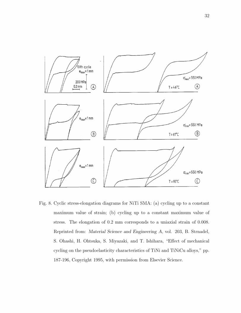
8 Cyclic stress-elongation diagrams for NiTi SMA: (a) cycling up to

a constant maximum value of strain; (b) cycling up to a constant

maximum value of stress. The elongation of 0.2 mm corresponds

to a uniaxial strain of 0.008. . . . . . . . . . . . . . . . . . . . . . . . 32

9 Schematic of minor hysteresis loops predicted by the current model

and experimentally observed. . . . . . . . . . . . . . . . . . . . . . . 50

10 Definition of the order of minor loop branches. . . . . . . . . . . . . . 51

11 Schematic of a uniaxial pseudoelastic test. . . . . . . . . . . . . . . . 60

12 Effect of the parameter ρ∆s0 on the stress-strain response during

forward phase transformation. . . . . . . . . . . . . . . . . . . . . . . 62

13 Effect of the parameter Y on the size of the hysteresis loop. . . . . . 63

xi

FIGURE Page

14 Normalized maximum transformation strain for thermally induced

phase transformation versus the applied stress: experimental data

for NiTi SMA (Lagoudas and Bo, 1999) and a polynomial least-

square fit. A polynomial of degree 5 is used. . . . . . . . . . . . . . . 65

15 Effect of the parameter Dd1 on the stress-strain response during


16 Effect of the parameter Dd2 on the stress-strain response during


17 Effect of the parameter γ on the minor loop curvature. The minor

loops occur due to incomplete forward phase transformation. . . . . . 70

18 Schematic of the BVP for uniaxial pseudoelastic SMA response;

(a) geometry and boundary conditions; (b) loading history. . . . . . . 86

19 Pseudoelastic uniaxial SMA response. . . . . . . . . . . . . . . . . . 87

20 Schematic of the BVP for uniaxial isobaric thermally-induced

transformation; (a) geometry and boundary conditions; (b) load-

ing history. . . . . . . . . . . . . . . . . . . . . . . . . . . . . . . . . 88

21 Strain versus temperature for different values of the applied stress. . 89

22 Schematic of the BVP for multiaxial loading of an SMA bar; (a)

geometry; (b) loading history; (c) finite element mesh and bound-

ary conditions. . . . . . . . . . . . . . . . . . . . . . . . . . . . . . . 90

23 Contour plot of the martensitic volume fraction in the SMA bar

at the end of the torsional loading. . . . . . . . . . . . . . . . . . . . 91

24 History of the axial and shear stress components during sequential

torsion-compression loading. . . . . . . . . . . . . . . . . . . . . . . . 92

25 History of the axial and shear transformation strain components

during sequential torsion-compression loading. . . . . . . . . . . . . . 93

26 History of the axial and shear stress components during simulta-

neous torsion-compression loading. . . . . . . . . . . . . . . . . . . . 94

xii

FIGURE Page

27 Stress-strain response of NiTi SMA to constant maximum stress

cycling: curves for the first and 50th cycles. . . . . . . . . . . . . . . 98

28 Plastic strain evolution during constant maximum stress cycling. . . 99

29 Stress-strain response of NiTi SMA to cycling up to a constant

maximum value of strain: curves for the first and 10th cycles. . . . . 100

30 Plastic strain evolution during constant maximum strain cycling. . . 101

31 Maximum value of the martensitic phase transformation ξmax dur-

ing constant maximum strain cycling. . . . . . . . . . . . . . . . . . 102

32 NiTi SMA torque tube: (a) geometry and finite element mesh;

(b) boundary conditions; (c) loading history for the first loading cycle. 103

33 Stress-strain response of NiTi SMA tube subjected to cycling tor-

sional loading: average shear stress over average shear strain. . . . . 104

34 Plastic strain evolution in NiTi SMA tube during cycling torsional

loading. . . . . . . . . . . . . . . . . . . . . . . . . . . . . . . . . . . 105

35 Change of the elastic stiffness during loading. . . . . . . . . . . . . . 109

36 Micrographs of a porous NiTi specimen (Tangaraj et al., 2000). . . . 122

37 (a) Global and local coordinate system; (b) principal axes of the

ellipsoidal inhomogeneity in the local coordinate system. . . . . . . . 124

38 Normalized effective elastic Young’s modulus for porous SMA. . . . . 125

39 Normalized effective elastic bulk modulus for porous SMA. . . . . . . 126

40 Normalized effective Young’s modulus calculated using the present

approach [equation (4.60)] compared with the Young’s modulus

calculated using the approach by Christensen (1991) [equation (4.63)]. 127

41 Schematic of the boundary-value problem for uniaxial loading of

a prismatic porous SMA bar. . . . . . . . . . . . . . . . . . . . . . . 129

42 Effective stress-strain response of a porous NiTi SMA bar. . . . . . . 130

xiii

FIGURE Page

43 Loading history for uniaxial porous SMA bar. . . . . . . . . . . . . . 131

44 Components of the macroscopic transformation strain as a func-

tion of the loading. . . . . . . . . . . . . . . . . . . . . . . . . . . . . 132

45 Components of the macroscopic transformation strain for the case

of equal stiffness of the austenite and martensite. . . . . . . . . . . . 134

46 Components of the macroscopic inelastic strain as a function of

the loading (both plastic and transformation strains are present). . . 135

47 Effective stress-strain response of a porous NiTi SMA bar (both

plastic and transformation strains are present). . . . . . . . . . . . . 136

48 Microphotograph of a small pore porous NiTi specimen. . . . . . . . 141

49 Microphotograph of a large pore porous NiTi specimen. . . . . . . . 142

50 DSC results for small pore porous NiTi alloy. . . . . . . . . . . . . . 143

51 DSC results for large pore porous NiTi alloy. . . . . . . . . . . . . . . 144

52 Stress-strain response of small pore porous NiTi alloy tested at 60�C. 145

53 Stress-strain response of large pore porous NiTi alloy tested at 60�C. 146

54 Elastic/phase transformation stress-strain response of small pore

porous NiTi alloy. . . . . . . . . . . . . . . . . . . . . . . . . . . . . 147

55 Comparison of the experimental elastic/phase transformation stress-

strain response of small pore porous NiTi alloy with the model

simulations. . . . . . . . . . . . . . . . . . . . . . . . . . . . . . . . . 149

56 Compressive loading of a porous NiTi SMA bar: (a) geometry;

(b) loading history; (c) boundary conditions. . . . . . . . . . . . . . . 153

57 Stress-strain response of a small pore porous NiTi SMA bar —

comparison between the experimental results and the model simulation.154

58 Plastic strain Ep versus accumulated detwinned martensitic vol-

ume fraction ζd for the small pore porous NiTi. . . . . . . . . . . . . 155

xiv

FIGURE Page

59 Stress-strain response of a large pore porous NiTi SMA bar —

comparison between the experimental results and the model simulation.156


ume fraction ζd for the large pore porous NiTi. . . . . . . . . . . . . 157

61 Stress-strain response of a large pore porous NiTi SMA bar —

last three loading cycles. . . . . . . . . . . . . . . . . . . . . . . . . . 158

62 Microcracking of the large pore porous NiTi SMA bar during me-

chanical loading. . . . . . . . . . . . . . . . . . . . . . . . . . . . . . 158


ume fraction ζd for the large pore porous NiTi using the modified

plastic strain evolution constants. . . . . . . . . . . . . . . . . . . . . 159

64 Stress-strain response of a large pore porous NiTi SMA bar using

the modified plastic strain evolution constants. . . . . . . . . . . . . 160

65 Schematic of the BVP for compression-torsion multiaxial loading

of a porous SMA bar: (a) boundary conditions; (b) loading histories. 162

66 History of the axial stress, shear stress and the martensitic volume

fraction during torsion-compression loading. . . . . . . . . . . . . . . 163

67 Contour plot of the martensitic volume fraction in the porous NiTi

SMA bar at the end of the torsional loading. . . . . . . . . . . . . . . 164

68 History of the axial stress, shear stress and the martensitic volume

fraction during torsion-compression loading. . . . . . . . . . . . . . . 166

69 Schematic of the BVP for compressive loading of a porous SMA

bar with constrained surfaces. . . . . . . . . . . . . . . . . . . . . . . 167

70 Stress-strain response of a small pore porous NiTi SMA bar show-

ing the three-dimensional effect during compressive loading. . . . . . 169

71 Contour plot of von Mises effective stress in the porous SMA bar

at the end of the compressive loading. . . . . . . . . . . . . . . . . . 170

72 Contour plot of the martensitic volume fraction in the porous

SMA bar at the end of the compressive loading. . . . . . . . . . . . . 171

1

CHAPTER I

INTRODUCTION

This chapter will cover some general aspects of Shape Memory Alloys (SMAs), in-

cluding a brief description of the martensitic phase transformation, some commonly

used SMAs, their thermomechanical characteristics and commercial applications. An

overview of the latest developments in the area of porous SMAs will be given. The

available constitutive models for fully dense SMAs as well as for porous SMAs will

also be reviewed. Finally, the objectives of the current research effort will be outlined.

1.1. General Aspects of Shape Memory Alloys

SMAs are metallic alloys which can recover permanent strains when they are heated

above a certain temperature. The key characteristic of all SMAs is the occurrence

of a martensitic phase transformation. The martensitic transformation is a shear-

dominant diffusionless solid-state phase transformation occurring by nucleation and

growth of the martensitic phase from a parent austenitic phase (Olson and Cohen,

1982). When an SMA undergoes a martensitic phase transformation, it transforms

from its high-symmetry, usually cubic, austenitic phase to a low-symmetry martensitic

phase, such as the monoclinic variants of the martensitic phase in a NiTi SMA.

The martensitic transformation possesses well-defined characteristics that distin-

guish it among other solid state transformations:

1. It is associated with an inelastic deformation of the crystal lattice with no

diffusive process involved. The phase transformation results from a cooperative

and collective motion of atoms on distances smaller than the lattice parameters.

The journal model is Mechanics of Materials.

2

The absence of diffusion makes the martensitic phase transformation almost

instantaneous (Nishiyama, 1978).

2. Parent and product phases coexist during the phase transformation, since it is

a first order transition, and as a result there exists an invariant plane, which

separates the parent and product phases. The lattice vectors of the two phases

possess well defined mutual orientation relationships (the Bain correspondences,

see Bowles and Wayman, 1972), which depend on the nature of the alloy.

3. Transformation of a unit cell element produces a volumetric and a shear strain

along well-defined planes. The shear strain can be many times larger than the

elastic distortion of the unit cell. This transformation is crystallographically

reversible (Kaufman and Cohen, 1958).

4. Since the crystal lattice of the martensitic phase has lower symmetry than that

of the parent austenitic phase, several variants of martensite can be formed from

the same parent phase crystal (De Vos et al., 1978).

5. Stress and temperature have a large influence on the martensitic transformation.

Transformation takes place when the free energy difference between the two

phases reaches a critical value (Delaey, 1990).

Due to their unique properties, SMAs have attracted great interest in various

fields of applications ranging from aerospace (Jardine et al., 1996; Liang et al., 1996)

and naval (Garner et al., 2000) to surgical instruments (Ilyin et al., 1995) and medical

implants and fixtures (Brailovski and Trochu, 1996; Gyunter et al., 1995). The SMAs

have been used in coupling devices (Melton, 1999), as actuators in a wide range of ap-

plications (Ohkata and Suzuki, 1999) as well as in medicine and dentistry (Miyazaki,

1999).

3

These applications have mostly benefited from the ability of the inherent shape

recovery characteristics of SMAs. In addition to the shape memory and pseudoelas-

ticity effects that SMAs possess, there is also the promise of using SMAs in making

high-efficiency damping devices that are superior to those made of conventional ma-

terials, partially due to their hysteretic response.

A relatively new area of applications utilizing the properties of SMAs is the area

of active composites (Lagoudas et al., 1994). The design of these composites involves

embedding SMA elements in the form of wires, short fibers, strips or particles into a

matrix material. Controlling the phase transformation of the SMA inclusions through

heating or cooling allows to control the overall behavior of the composite and change

its macroscopic properties (Birman, 1997).

1.2. Characteristics of the Martensitic Transformation in Polycrystalline Shape Mem-

ory Alloys

The martensitic transformation (austenite-to-martensite) occurs when the free energy

of martensite becomes less than the free energy of austenite at a temperature below

a critical temperature T0 at which the free energies of the two phases are equal.

However, the transformation does not begin exactly at T0 but, in the absence of

stress, at a temperature M0s (martensite start), which is less than T0. The free energy

necessary for nucleation and growth is responsible for this shift (Delaey, 1990). The

transformation continues to evolve as the temperature is lowered until a temperature

denoted M0f is reached. For SMAs, the temperature difference M0s −M0f is small

compared to that for the martensitic transformation in ferrous alloys (∼ 40�C for

SMAs versus ∼ 200�C for ferrous alloys). This temperature difference M0s −M0f is

an important factor in characterizing shape memory behavior.

4

When the SMA is heated from the martensitic phase in the absence of stress,

the reverse transformation (martensite-to-austenite) begins at the temperature A0s

(austenite start), and at the temperature A0f (austenite finish) the material is fully

austenite. The equilibrium temperature T0 is in the neighborhood of (M0s +A0f)/2.

The spreading of the cycle (A0f – A0s) is due to stored elastic energy, whereas the

hysteresis (A0s – M0f ) is associated with the energy dissipated during the transfor-

mation.

Due to the displacive character of the martensitic transformation, applied stress

plays a very important role. During cooling of the SMA material below tempera-

ture M0s in absence of applied stresses, the variants of the martensitic phase arrange

themselves in a self-accommodating manner through twinning, resulting in no ob-

servable macroscopic shape change (see the stress-temperature diagram shown in

Figure 1). By applying mechanical loading to force martensitic variants to reorient

(detwin) into a single variant, large macroscopic inelastic strain is obtained. Af-

ter heating to a higher temperature, the low-symmetry martensitic phase returns to

its high-symmetry austenitic phase, and the inelastic strain is thus recovered. The

martensitic phase transformation can also be induced by pure mechanical loading

while the material is in the austenitic phase, in which case detwinned martensite is

directly produced from austenite by the applied stress (Stress Induced Martensite,

SIM) at temperatures above M0s (Wayman, 1983).

As a result of the martensitic phase transformation, the stress-strain response

of SMAs is strongly non-linear, hysteretic, and a very large reversible strain is ex-

hibited. This behavior is strongly temperature-dependent and very sensitive to the

number and sequence of thermomechanical loading cycles. In addition, microstruc-

tural aspects have considerable influence on the stress-strain curve and on the strain-

temperature curves. In polycrystals, the differences in crystallographical orientation

5

T

�

0 fM

0sA

0sM

0 fA

0 ,s tM

0 ,f tM

Detwinned

martensite

Austenite

Twinned

martensite

Plastic deformation

Fig. 1. SMA stress-temperature phase diagram.

among grains produce different transformation conditions in each grain. The polycrys-

talline structure also requires the satisfaction of geometric compatibility conditions

at grain boundaries, in addition to compatibility between austenite and the different

martensitic variants. Thus, the martensitic transformation is progressively induced

in the different grains and, as opposed to the single crystal case, no well-defined onset

of the transformation is observed. In addition, the hysteresis size increases, and the

macroscopic transformation strain decreases.

The austenite-to-martensite transformation is accompanied by the release of heat

corresponding to the transformation enthalpy (exothermic phase transformation).

The martensite-to-austenite (reverse) transformation is an endothermic phase trans-

6

formation accompanied by absorption of thermal energy. For a given temperature,

the amount of heat is proportional to the volume fraction of the transformed material.

This heat release (heat absorption) is utilized by the Differential Scanning Calorime-

try (DSC) method to measure the transformation temperatures. Other methods, as

the measurement of the electrical resistivity, internal friction, thermoelectric power

and the velocity of sound are also used in establishing the values of the transformation

temperatures (Jackson et al., 1972).

The key effects of SMAs associated with the martensitic transformation, which

are observed according to the loading path and the thermomechanical history of

the material are: pseudoelasticity, one-way shape memory effect and two-way shape

memory effect. In this section, the characteristics associated with these classes of

behavior are presented, and the various strain mechanisms behind these effects are

described.

1.2.1. Shape Memory Effect

An SMA exhibits the Shape Memory Effect (SME) when it is deformed while in the

martensitic phase and then unloaded while still at a temperature below M0f . If it is

subsequently heated above A0f it will regain its original shape by transforming back

into the parent austenitic phase. The nature of the SME can be better understood by

following the process described above in a stress-temperature phase diagram schemat-

ically shown in Figure 2. The parent austenitic phase (indicated by A in Figure 2)

in the absence of applied stress will transform upon cooling to multiple martensitic

variants (up to 24 variants for the cubic-to-monoclinic transformation) in a random

orientation and in a twinned configuration (indicated by B). As the multivariant

martensitic phase is deformed, a detwinning process takes place, as well as growth of

certain favorably oriented martensitic variants at the expense of other variants. At

7

the end of the deformation (indicated by C) and after unloading it is possible that

only one martensitic variant remains (indicated by D). Upon heating, when tempera-

ture reaches A0s, the reverse transformation begins to take place, and it is completed

at temperature A0f . The highly symmetric parent austenitic phase (usually with

a cubic symmetry) forms only one variant, and thus the original shape (before de-

formation) is regained (indicated by E). Note that subsequent cooling will result in

multiple martensitic variants with no substantial shape change (self-accommodated

martensite). Also, note in Figure 2 that, in going from A to B many variants will

start nucleating from the parent phase, while in going from D to E there is only

one variant of the parent phase that nucleates from the single remaining martensitic

variant indicated by D.

The stress-free cooling of austenite produces a complex arrangement of several

variants of martensite. Self-accommodating growth is obtained such that the average

macroscopic transformation strain equals zero (Otsuka and Wayman, 1999b; Saburi,

1999; Saburi et al., 1980), but the multiple interfaces present in the material (bound-

aries between the martensite variants and twinning interfaces) are very mobile. This

great mobility is at the heart of the SME. Movement of these interfaces accompanied

by detwinning is obtained at stress levels far lower than the plastic yield limit of

martensite. This mode of deformation, called reorientation of variants, dominates at

temperatures lower than M0f .

The above described phenomenon is called one-way shape memory effect (or

simply, shape memory effect) because the shape recovery is achieved only during

heating. The first step in the loading sequence induces the development of the self-

accommodated martensitic structure, and no macroscopic shape change is observed.

During the second stage, the mechanical loading in the martensitic phase induces

reorientation of the variants and results in a large inelastic strain, which is not recov-

8

T

�

0 fM

0sA

0sM

0 fA AB

C

ED

Fig. 2. Schematic representation of the thermomechanical loading path demonstrating

the shape memory effect in an SMA.

ered upon unloading (Figure 3). Only during the last step the reverse transformation

induced by heating recovers the inelastic strain. Since martensite variants have been

reoriented by stress, the reversion to austenite produces a large transformation strain

having the same amplitude but the opposite direction with the inelastic strain, and

the SMA returns to its original shape of the austenitic phase.

1.2.2. Pseudoelasticity

The pseudoelastic behavior of SMAs is associated with recovery of the transformation

strain upon unloading and encompasses both superelastic and rubberlike behavior (Ot-

suka et al., 1976; Otsuka and Wayman, 1999a). The superelastic behavior is observed

9

�

�

T

Cooling

Detwinning

Heating/Recovery

Fig. 3. Schematic of a stress-strain-temperature curve showing the shape memory

effect.

during loading and unloading above A0s and is associated with stress-induced marten-

site and reversal to austenite upon unloading. When the loading and unloading of

the SMA occurs at a temperature above A0s, partial transformation strain recovery

takes place. When the loading and unloading occurs above A0f , full recovery upon

unloading takes place. Such loading path in the stress-temperature space is schemat-

ically shown in Figure 4. Initially, the material is in the austenitic phase (point A).

The simultaneous transformation and detwinning of the martensitic variants starts at

point B and results in fully transformed and detwinned martensite (point C). Upon

10

T

�

0 fM

0sA

0sM

0 fA

A

C

D

B

E

Fig. 4. Schematic of a thermomechanical loading path demonstrating pseudoelastic

behavior of SMAs.

unloading, the reverse transformation starts when point D is reached. Finally, at the

end of the loading path (point E) the material is again in the austenitic phase.

If the material is in the martensitic state and detwinning and twinning of the

martensitic variants occur upon loading and unloading, respectively, by reversible

movement of twin boundaries, this phenomenon is called rubberlike effect (Otsuka

and Wayman, 1999a). The rubberlike effect is less common, while the superelastic

effect is very common in almost all SMAs.

Three distinct stages are observed on the uniaxial stress-strain curve representing

the superelastic behavior of an SMA, schematically shown in Figure 5. For stresses

11

below σMs, the material behaves in a purely elastic way. As soon as the critical stress is

reached, forward transformation (austenite-to-martensite) initiates and stress-induced

martensite starts forming. During the formation of SIM large transformation strains

are generated (upper plateau of stress-strain curve in Figure 5). When the applied

stress reaches the value σMf the forward transformation is completed and the SMA

is in the martensitic phase. For further loading above σMf the elastic behavior of

martensite is observed. Upon unloading, the reverse transformation initiates at a

stress σAs and completes at a stress σAf . Due to the difference between σMf and

σAs and between σMs and σAf a hysteretic loop is obtained in the loading/unloading

stress-strain diagram. Increasing the test temperature results in an increase of the

values of critical transformation stresses, while the general shape of the hysteresis

loop remains the same.

��Mf

��Ms

��Af

��As

�

�

Fig. 5. Schematic of the superelastic behavior of SMAs.

12

Upon cooling under a constant applied stress from a fully austenitic state, it is

observed that the transformation is characterized by a martensite start temperature

Mσs and a martensite finish temperature Mσf , which are functions of the applied

stress. Macroscopic transformation strain obtained in that way (Figure 6) is a result

of martensite formation and detwinning of the martensitic variants due to the applied

load. The transformation strain is several orders of magnitude greater than the

thermal strain corresponding to the same temperature difference required for the

phase transformation. A hysteresis loop is observed for the cooling/heating cycle as

shown in Figure 6 due to the fact that the reverse transformation begins and ends at

different temperatures than the forward transformation does.

1.2.3. Behavior of SMAs Undergoing Cyclic Loading

The superelastic behavior described in Section 1.2.2 constitutes an approximation to

the actual behavior of SMAs under applied stress. In fact, only a partial recovery of

the transformation strain induced by the applied stress is observed. A small residual

strain remains after each unloading. Further cooling of the material, in the absence of

applied stress, is now related to the occurrence of a macroscopic transformation strain

contrary to what is observed in the SMA material before cycling. Experimental results

on the behavior of SMAs undergoing cyclic loading have been presented by Bo and

Lagoudas (1999a); Kato et al. (1999); Lim and McDowell (1999, 1994); McCormick

and Liu (1994); Strnadel et al. (1995a,b) and Sehitoglu et al. (2001), among others.

The thermomechanical cycling of the SMA material results in training process as

first observed by Perkins (1974). Different training sequences can be used (Contardo

and Guenin, 1990; Miller and Lagoudas, 2001), i.e., by inducing a non-homogeneous

plastic strain (torsion, flexion) at a martensitic or austenitic phase; by aging under

applied stress, in the austenitic phase, in order to stabilize the parent phase, or

13

fM

� s

M� s

A� f

A�

T

�

Fig. 6. Schematic of isobaric thermally induced transformation behavior of SMAs.

in the martensitic phase, in order to create a precipitant phase (Ni-Ti alloys); by

thermomechanical, either superelastic or thermal cycles.

The main result of the training process is the development of Two-Way Shape

Memory Effect (TWSME). In the case of TWSME, a shape change is obtained both

during heating and cooling. The solid exhibits two stable shapes: a high-temperature

shape in austenite and a low-temperature shape in martensite. Transition from the

high-temperature shape to the low-temperature shape (and reverse) is obtained with-

out any applied stress assistance.

14

In contrast with the previously discussed properties of SMAs (superelasticity,

one-way shape memory) that are intrinsic, the TWSME is an acquired characteristic.

In the heart of the TWSME is the generation of internal stresses and creation of

permanent defects during training. The process of training leads to the preferential

formation and reversal of a particular martensitic variant under the applied load.

Generation of permanent defects eventually creates a permanent internal stress state,

which allows for the formation of the preferred martensitic variant in the absence of

the external load.

Another effect of the training cycle is the development of macroscopically ob-

servable plastic strain. The magnitude of this strain is comparable to the magnitude

of the recoverable transformation strain. The training also leads to secondary effects,

like change in the transformation temperatures, change in the hysteresis size and de-

crease in the macroscopic transformation strain. These effects are similar to those

observed during thermomechanical fatigue tests (Rong et al., 2001). It is important

to define optimal conditions of training, because an insufficient number of training

cycles produces a non-stabilized two-way memory effect and over-training generates

unwanted effects that reduce the efficiency of training (Stalmans et al., 1992).

1.3. Porous Shape Memory Alloys — Characteristics and Applications

Driven by biomedical applications, recent emphasis has been given to porous SMAs.

The possibility of producing SMAs in porous form opens new fields of application,

including reduced weight and increased biocompatibility. Perhaps the most successful

application of porous SMAs to this date is their use as bone implants (Ayers et al.,

1999; Shabalovskaya et al., 1994; Simske et al., 1997). One of the main reasons for

such a success is the biocompatibility of the NiTi alloys used in the above cited works.

15

In addition, the porous structure of the alloys allows ingrowth of the tissue into the

implant.

In the last several years since the fabrication techniques for porous SMAs have

been established, additional applications have also been considered. The potential

applications of porous SMAs utilize their ability to carry significant loads. Beyond

the energy absorption capability of dense SMA materials, porous SMAs offer the

possibility of higher specific damping capacity under dynamic loading conditions.

One of the applications, which utilizes the energy absorption capabilities of the porous

SMAs, is the development of effective dampers and shock absorbing devices. It has

been demonstrated that a significant part of the impact energy is absorbed (Lagoudas

et al., 2000a). The reason for such high energy absorption is the sequence of forward

and reverse phase transformations in the SMA matrix. In addition to the inherent

energy dissipation capabilities of the SMA matrix, it is envisioned that the pores will

facilitate additional absorption of the impact energy due to wave scattering. This

phenomenon has been studied in great detail by Sabina et al. (1993); Sabina and

Willis (1988) and Smyshlyaev et al. (1993a,b). However, the effect of wave scattering

in porous SMAs has not been investigated yet.

Another advantage of the porous SMAs over their fully dense counterparts is

the possibility to fabricate them with gradient porosity. This porosity gradient of-

fers enormous advantage in applications involving impedance matching at connecting

joints and across interfaces between materials with dissimilar mechanical properties.

The use of such porous SMA connecting elements will prevent failure due to wave

reflections at the interfaces, while at the same time providing the connecting joint

with energy absorption capabilities. Also currently of great interest is the use of

porous SMAs in various vibration isolation devices. It is envisioned that such devices

will find applications in various fields ranging from isolation of machines and equip-

16

ment to isolation of payloads during launch of space vehicles. To increase the energy

absorption capabilities a second phase, which would fill the pores can be added. It

should be noted that these latest developments are still being actively researched and

have not yet been used in commercial applications.

Different fabrication techniques for producing porous SMAs have been estab-

lished. While some of the works focus on fabrication of porous SMAs by injecting a

gas into a melt (Hey and Jardine, 1994), most of the research work on fabrication of

porous SMAs has focused on using powder metallurgy techniques (Goncharuk et al.,

1992; Itin et al., 1994; Li et al., 1998; Martynova et al., 1991; Shevchenko et al., 1997;

Tangaraj et al., 2000; Vandygriff et al., 2000; Yi and Moore, 1990). Different fabrica-

tion techniques for producing porous SMAs from elemental powders have been used.

Some of the difficulties that may be encountered with the use of elemental powders

include contamination from oxides and the formation of other intermetallic phases.

On the other hand, producing pre-alloyed NiTi powder requires processing techniques

which are both difficult and expensive due to the hardness of the alloy.

Techniques that are currently being used to produce porous NiTi from elemental

powders include self-propagating high-temperature synthesis, conventional sintering,

and sintering at elevated pressures via a Hot Isostatic Press (HIP). Some advantages of

sintering at elevated pressure include shorter heating times than conventional sintering

and the ability to produce near net shape objects that require less time to machine.

The current work uses porous NiTi fabricated using the HIPping technique. The

process is presented in detail by Vandygriff et al. (2000) and is not discussed here.

Two different porous NiTi alloys were obtained: at lower fabrication temperature

(≈ 940�C) a porous material with smaller pore sizes is obtained, while for higher

temperature (≈ 1000�C) the sizes of the pores are significantly larger. Micrographs

of both large and small pore specimens are shown in Figure 7.

17

Pores

NiTi

1 mm1 mm

50 �m250 �m

Fig. 7. Micrographs of porous NiTi specimens.

1.4. Review of the Models for Dense and Porous SMAs

During the last two decades significant advancements in the area of constitutive mod-

eling of SMAs have been reported. In addition to the models developed for fully dense

SMAs, models for porous SMAs have started to appear during recent years. Achieve-

ments in both of these areas are summarized in the following subsections.

1.4.1. Modeling of Fully Dense SMAs

The area of constitutive modeling of fully dense SMAs has been a topic of many

research publications in recent years. The majority of the constitutive models re-

18

ported in the literature can be formally classified to belong to one of the two groups:

micromechanics-based models and phenomenological models. Representative works

from both of these groups are reviewed in a sequel.

The essence of the micromechanics-based models is in the crystallographic mod-

eling of a single crystal or grain and further averaging of the results over a represen-

tative volume element (RVE) to obtain a polycrystalline response of the SMA. Such

models have been presented in the literature by different researchers. As an exam-

ple, the micromechanics-based model based on the analysis of phase transformation

in single crystals of copper-based SMAs has been presented by Patoor et al. (1988,

1994, 1996). The behavior of a polycrystalline SMA is modeled by utilizing the model

for single crystals and using the self-consistent averaging method to account for the

interactions between the grains. A micromechanical model for SMAs which is able

to capture different effects of SMA behavior such as superelasticity, shape memory

effect and rubber-like effect has been presented by Sun and Hwang (1993a,b). In

their work, the evolution of the martensitic volume fraction is obtained by balanc-

ing the internal dissipation during the phase transformation with the external energy

output. One of the recent micromechanical models for SMA has been presented by

Gao et al. (2000a,b). The advantage of the crystallographical models is their ability

to predict the material response using only the crystallographical parameters (e.g.,

crystal lattice parameters). Thus, their use provides valuable insight on the phase

transformation process on the crystal level. Their disadvantage, however, is in the

large number of numerical computations required to be performed. Thus the use of

such models for modeling structural response is not feasible.

Contrary to the crystallographical models, in the case of the phenomenological

models a macroscopic energy function is proposed and used in conjunction with the

second law of thermodynamics to derive constraints on the constitutive behavior of

19

the material. Thus the resulting model does not directly predict the behavior of the

material on microscopic level, but the effective behavior of the polycrystalline SMA.

These models have the advantage of being easily integrated into an existing structural

modeling system, e.g., using the finite element method.

Some of the early three-dimensional models from this group were derived by

generalizing the one-dimensional results, such as the models by Boyd and Lagoudas

(1994); Liang and Rogers (1992) and Tanaka et al. (1995). In a publication by

Lagoudas et al. (1996) it has been shown that various phenomenological models can

be unified under common thermodynamical formulation. The differences between the

models arise due to the specific choice of transformation hardening function. More

recent phenomenological models have also been presented by Auricchio et al. (1997);

Leclercq and Lexcellent (1996); Levitas (1998); Reisner et al. (1998); Rengarajan et al.

(1998) and Rajagopal and Srinivasa (1999). In a recent work Qidwai and Lagoudas

(2000b) presented a general thermodynamic framework for phenomenological SMA

constitutive models, which for different choice of the transformation function can be

tuned to capture different effects of the martensitic phase transformation, such as

pressure dependance and volumetric transformation strain.

In addition to modeling of the development of transformation strain during

martensitic phase transformation, several other modeling issues have also been topics

of intensive research. One of the most important problems recently addressed by

the researchers is the behavior of SMAs under cycling loading. During cycling phase

transformation a substantial amount of plastic strains is accumulated. In addition,

the transformation loop evolves with the number of cycles and TWSME is developed.

Based on the experimental observations researchers have attempted to create models

able to capture the effects of cycling loading. One-dimensional models for the be-

havior of SMA wires under cycling loading have been presented by Lexcellent and

20

Bourbon (1996); Lexcellent et al. (2000); Tanaka et al. (1995) and Abeyaratne and

Kim (1997), among others. A three-dimensional formulation is given by Fischer et al.

(1998). Their model defines a transformation function to account for the development

of the martensitic phase transformation and a separate yield function to account for

the development of plasticity. However, neither the identification of the material pa-

rameters nor implementation of the model is presented in that work. One of the most

recent works on the cyclic behavior of SMA wires has been presented in a series of

papers by Bo and Lagoudas (1999a,b,c) and Lagoudas and Bo (1999). In that work

most of the issues regarding behavior of SMA wires under cycling loading, including

the development of TWSME, have been addressed and the results compared with the

experimental data.

While most of the constitutive models for dense SMAs assume that the mate-

rial exhibits rate-independent behavior, a notable exception from this is the model

developed by Abeyaratne and Knowles (1993) and Abeyaratne et al. (1993, 1994).

Abeyaratne and Knowles (1994a,b, 1997) have applied their model to model the prop-

agation of phase boundaries in an SMA rod.

1.4.2. Modeling of Porous SMAs

In this subsection the models potentially applicable to modeling of porous SMAs

are reviewed. Since the porous SMA can be viewed as a composite with an SMA

matrix and the pores as the second phase, the models presented for active SMA-

based composites are also reviewed.

A great number of research papers have appeared in the literature devoted to

modeling of porous materials. While some of them deal with the elastic response of

the materials, the inelastic and more specifically, plastic behavior has also been a topic

of research investigations. Different aspects of modeling of porous and cellular solids

21

are presented by Green (1972); Gurson (1977); Jeong and Pan (1995) and Gibson

and Ashby (1997), among others. The idea behind the works of Green (1972) and

Gurson (1977) is to derive a macroscopic constitutive model with an effective yield

function for the onset of plasticity. In addition, the work of Gurson (1977) deals with

the nucleation and evolution of porosity during loading. A comprehensive study on

porous and cellular materials is presented in the book by Gibson and Ashby (1997).

However, most of the modeling in that work is presented in the context of a single cell

modeling for high-porosity materials. The cells are modeled using the beam theory

to account for the ligaments between the pores. In addition, the walls of the pores in

the case of closed cell porosity are modeled as membranes. Both the elastic properties

as well as the initiation of plasticity are modeled.

Since the emerging of the SMA-based active composites their modeling has been

the subject of a number of research papers. One approach to modeling of these

composites is to extend the theories for linear composites, which is well developed

(e.g., see the review papers by Willis, 1883, 1981 and the monograph by Christensen,

1991).

Some of the modeling work on SMA composites has been performed using the

approximation of an existence of a periodic unit cell (Achenbach and Zhu, 1990;

Lagoudas et al., 1996; Nemat-Nasser and Hori, 1993). One of the recent works on

porous SMAs also used the unit cell approximation to evaluate the properties of

porous SMAs (Qidwai et al., 2001). Even though the existence of periodic arrange-

ment of pores in a real porous SMA material is an approximation, this assumption

provides insight into global material behavior in the form of useful limiting values for

the overall properties. Additionally, an approximate local variation of different field

variables like stress and strain indicating areas of concentration due to porosity can be

obtained. These results may provide design limitations in order to minimize or even

22

avoid micro-buckling, plastic yielding and consequently loss of phase transformation

capacity over number of loading cycles. The assumption of periodicity and symmetry

boundary conditions reduce the analysis of the porous SMA material to the analysis

of a unit cell. In addition, appropriate loading conditions need to be applied, which

do not violate the symmetry of the problem (Qidwai et al., 2001). In a recent work

DeGiorgi and Qidwai (2001) have investigated the behavior of porous SMA using a

mesoscale representation of the porous structure. In addition, DeGiorgi and Qidwai

(2001) have studied the effect of filling the pores with a second polymeric phase.

The variational techniques have initially been used to establish bounds on the

properties of linear composites. Various bounds have been presented in the literature,

ranging from the simplest Reuss and Voigt bounds (Christensen, 1991; Paul, 1960)

to Hashin–Shtrikman bounds (Hashin and Shtrikman, 1963; Walpole, 1966). The

variational techniques have also been extended to obtain estimates for the behavior

of non-linear composites. Most notably, in the works of Talbot and Willis (1985) and

Ponte Castaneda (1996) bounds for the properties of non-linear composites have been

reported.

Micromechanical averaging techniques have also been used to determine the av-

eraged macroscopic composite response. Among the micromechanics averaging meth-

ods, the two most widely used are the self-consistent method and the Mori–Tanaka

method. Both approaches are based on the presumption that the effective response of

the composite can be obtained by considering a single inhomogeneity embedded in an

infinite matrix. According to the self-consistent method (Budiansky, 1965; Hershey,

1954; Hill, 1965; Kroner, 1958) the interactions between the inhomogeneities are taken

into account by associating the properties of the matrix with the effective properties

of the composite, i.e., embedding the inhomogeneity in an effective medium. Some

self-consistent results for spherical pores in an incompressible material are presented

23

by Budiansky (1965). Contrary to this approach, the Mori–Tanaka method initially

suggested by Mori and Tanaka (1973) and further developed by Weng (1984) and

Benveniste (1987) takes into account the interactions between the inhomogeneities

by appropriately modifying the average stress in the matrix from the applied stress,

while the properties of the matrix are associated with the real matrix phase. These

averaging techniques can also be used to determine the averaged macroscopic response

of the porous material with random distribution of pores. In this case the material is

treated as a composite with two phases: dense matrix and pores.

Recently, both averaging approaches have been applied to obtain effective proper-

ties of composites with inelastic phases. For example, a variant of the self-consistent

method using incremental formulation (Hutchinson, 1970) has been used to model

composites undergoing elastoplastic deformations. Lagoudas et al. (1991) have used

an incremental formulation of the Mori–Tanaka method to obtain the effective proper-

ties of a composite with an elastoplastic matrix and elastic fibers. Boyd and Lagoudas

(1994) have applied the Mori–Tanaka micromechanical method to model the effective

behavior of a composite with elastomeric matrix and SMA fibers and have obtained

the effective transformation temperatures for the composite. In a different work,

Lagoudas et al. (1994) have applied the incremental Mori–Tanaka method to model

the behavior of a composite with elastic matrix and SMA fibers. Another group of

researchers (Cherkaoui et al., 2000) has applied the self-consistent technique to ob-

tain the effective properties of a composite with elastoplastic matrix and SMA fibers.

A two-level micromechanical method has been presented by Lu and Weng (2000),

where the SMA constitutive behavior has been derived at the microscopic level and

the overall composite behavior has been modeled at the mesoscale level using the

Mori–Tanaka method.

In summary, it should be mentioned that all of the methods have their advantages

24

as well as disadvantages. The approach offered by Gibson and Ashby (1997) requires

the existence of a very regular pore structure and is applicable only for high-porosity

materials (porosity on the order of 90%). Similarly, the unit cell methods are accurate

for regular pore structure. The advantage of these methods is that they can accurately

model the stress distribution in the vicinity of the pore boundaries and are not limited

by the shape of the pores. The difficulty associated with these methods is their

computational intensity which makes them not feasible for structural calculations. On

the other hand, the phenomenological approach, presented by Green (1972); Gurson

(1977) and Jeong and Pan (1995) can easily be adapted to model large structural

systems. Its disadvantage is the fact that the effect of pore shapes and orientations

on the properties of the porous SMA cannot easily be taken into account.

The micromechanical averaging techniques combine some of the advantages of

both of the approaches. While the pore shape choices are limited to ellipsoids, pores

with any orientations can easily be taken into account. By varying the ratio of the

axes of the ellipsoid, different shapes (e.g., cylinders, prolate and oblate spheroids,

cracks) can be represented. The micromechanical averaging schemes can also easily

be implemented numerically to model structural response of complex systems.

1.5. Outline of the Present Research

The research effort presented in this work is divided into two major parts. The

first part is devoted to the constitutive modeling of fully dense SMAs using a phe-

nomenological constitutive model. The second part describes the modeling of porous

SMAs using micromechanical averaging techniques. Thus, the research objectives are

summarized as follows:

25

1. Develop a three-dimensional constitutive model for fully dense SMAs

which is able to account for non-linear transformation hardening, si-

multaneous development of transformation and plastic strains during

phase transformation and evolution of the material behavior during

cyclic loading. The experimental observations for the mechanical behavior of

porous SMAs in the pseudoelastic regime have shown that a significant part of

the developed strain is not recovered upon unloading. Even upon heating the

specimen in a furnace with no load applied this unrecoverable strain remains

unchanged. Thus, the development of this strain has been attributed to plas-

ticity (Lagoudas and Vandygriff, 2002). As described in the literature review,

similar observations are presented in the literature for fully dense SMAs. There-

fore, to be able to successfully model the behavior of porous SMAs, a model

for the dense SMA matrix which is able to capture the development of plastic

strains is needed. However, the majority of such models found in the litera-

ture have one-dimensional formulation. Due to the three-dimensional effects

existing in a porous SMA, its successful modeling requires a three-dimensional

model. A three-dimensional model for sequential transformation and plasticity

is presented by Fischer et al. (1998). However, the current work will focus on

modeling of simultaneous phase transformation and plasticity, i.e., development

of plastic strains during the phase transformation. The three-dimensional model

development will follow the methodology presented for the one-dimensional

case by Bo and Lagoudas (1999a,b,c) and Lagoudas and Bo (1999). Since the

above-mentioned works describe the behavior of SMAs undergoing temperature-

induced transformation, the necessary modifications to adapt the formulation

for the case of stress-induced martensitic transformation will be made.

26

2. Develop a macroscopic thermomechanical constitutive model for the

porous SMA material using micromechanical averaging techniques.

The current work will extend micromechanical averaging techniques for inelas-

tic composites to establish a macroscopic constitutive model for the porous

SMA material. The micromechanical methods based on Eshelby’s solution will

be used in incremental formulation. The response of the porous SMA will be

deducted using the properties of the dense SMA and information about pore

shape, orientation and volume fraction. Analytical expressions for the overall

elastic and tangent stiffness of the porous SMA material will be derived and

an evolution equation for the overall transformation strain will also be derived.

The derivations will first be given for the more general case of a two-phase com-

posite with rate-independent constituents. After the derivation of the general

expressions, the properties of the porous SMA material will be obtained by us-

ing the constitutive model for dense SMA developed in this work to model the

matrix, and treating the inhomogeneities as elastic phases with stiffness equal

to zero.

3. Provide a detailed procedure for the estimation of the material pa-

rameters for the model using experimental data and demonstrate the

capabilities of the model by comparing the model simulations to the

results from the available experiments. The material parameters used

by the model in characterizing the porous SMA material will be identified and

their values will be estimated using the experimental results for porous NiTi

SMA. Porous NiTi alloys fabricated from elemental powders will be used in this

research effort. Two different porous SMAs will be tested under compressive

loading. The complete set of material parameters for both alloys will be pre-

27

sented. Various loading paths will be simulated using the obtained parameters.

4. Develop a numerical implementation of the thermodynamical consti-

tutive model for both dense and porous SMAs. The numerical imple-

mentation of the model for dense SMAs using return mapping algorithms will

be presented. The numerical implementation of the model for porous SMAs will

be accomplished using the implementation of the model for dense SMAs and the

direct iteration method. The derivations of the numerical implementation will

be given in a sufficiently general form suitable for any displacement-based nu-

merical code. The approach presented by Qidwai and Lagoudas (2000a) for the

fully dense SMA model with a polynomial hardening function will be followed.

The model will be implemented as a user-material constitutive subroutine for

the finite element package ABAQUS.

The content of each chapter of this work is as follows: in Chapter II the deriva-

tions of the fully dense SMA constitutive model are given. The chapter contains

sections on the identification of the internal state variables, their evolution and on

the estimation of the material parameters. The numerical implementation of the

model is presented in Chapter III, which also contains a section on the comparison

of the model simulations with the experimental results. Chapter IV proceeds with

the derivation of the micromechanical averaging model for porous SMAs. Detailed

derivations of the effective elastic stiffness, effective tangent stiffness and the evolu-

tion of the effective inelastic strain is presented. The numerical implementation of

the model for porous SMAs is discussed in Chapter V. The estimation of the material

parameters for the porous NiTi SMA and results for numerical simulation of various

boundary value problems for porous SMA bars are also presented in Chapter V. A

summary of the research effort presented in this work as well as recommendations for

28

future work on the subject are presented in Chapter VI.

The direct notation is adopted in this work. Capital bold Latin letters represent

fourth-order tensors (effective stiffness L, compliance M, etc.) while bold Greek

letters are used to denote second-order tensors — lower case for the local quantities

(stress σ, strain ε) and capital for the macroscopic quantities (effective stress Σ,

strain E). Regular font is used to denote scalar quantities as well as the components

of the tensors. Multiplication of two fourth-order tensors A and B is denoted by

AB = (AB)ijkl ≡ AijpqBpqkl, while the operation “:” defines contraction of two

indices when a fourth-order tensor acts on a second-order one, A : E ≡ Aijk�Ek�.

29

CHAPTER II

THERMOMECHANICAL CONSTITUTIVE MODELING

OF FULLY DENSE POLYCRYSTALLINE SHAPE MEMORY ALLOYS

In this chapter the derivation of a three-dimensional thermomechanical constitutive

model for SMAs undergoing cyclic loading which results in simultaneous development

of transformation and plastic strains will be presented. The model is an extension of

the one-dimensional model presented by Bo and Lagoudas (1999a,b,c) and Lagoudas

and Bo (1999) to three dimensions. Of most interest in this model is the evolution of

plastic strains during stress-induced martensitic phase transformation as well as the

non-linear transformation hardening.

While the basic ideas for the formulation of the current model have been pre-

sented by many authors in the literature and specifically by Lagoudas and Bo (1999)

and Bo and Lagoudas (1999a,b,c) there are several important distinctions between

the model presented here and the one reported by Bo and Lagoudas (1999b) which

must be pointed out. The major difference between the two models is that the current

model is capable of simulating three-dimensional behavior of SMAs while the model by

Bo and Lagoudas (1999b) has only been implemented for the case of one-dimensional

SMA wires. While some of the applications of SMAs can utilize the one-dimensional

model, an increasing number of applications requires three-dimensional modeling.

As an example, smart wing design, presented by Jardine et al. (1996) utilizes SMA

torque tubes and their successful modeling requires three-dimensional formulation.

The three-dimensional capabilities of the model are demonstrated in Section 3.4.1

where a model is used to simulate the behavior of an SMA torque tube. The three-

dimensional formulation is essential for the further application of micromechanical

averaging techniques for porous SMAs, which is the ultimate goal of the current

30

study.

Another difference between the current model and the model by Bo and Lagoudas

(1999b) is the way of calibrating the model parameters. While the previous publi-

cations (Bo and Lagoudas, 1999a,b,c; Lagoudas and Bo, 1999) have been devoted

exclusively to characterizing the behavior of SMA wires undergoing temperature-

induced phase transformation, the current work is aimed at characterizing the SMAs

undergoing stress-induced phase transformation. Thus, the procedure for estimation

of the material parameters, presented in Section 2.7 utilizes data for SMAs undergo-

ing stress-induced phase transformation. While the present model can still be used

to model temperature-induced phase transformation, to obtain accurate results some

of the material parameters may need to be re-calibrated. The evolution equation

for the plastic strain used here also differs from the expression presented by Bo and

Lagoudas (1999a). The use of the current expression is motivated by the experi-

mental observations for the evolution of plastic strains during stress-induced phase

transformation.

Finally, the functional form of the back stress different from the one used by Bo

and Lagoudas (1999b) is used in the current work. As explained earlier, the current

functional form of the back stress simplifies the estimation of the material parameter

and it is simpler to numerically implement, than the one used by Bo and Lagoudas

(1999b). In addition, evolution equations for the back stress material parameters used

here are also different from the ones presented by Bo and Lagoudas (1999a). While the

evolution of these parameters in the work of Bo and Lagoudas (1999a) depends on the

effective accumulated plastic strain, in this work it is connected to the accumulated

detwinned martensitic volume fraction. Such a modification significantly simplifies

the calibration of the model.

31

2.1. Experimental Observations for Polycrystalline SMAs Undergoing Cyclic Load-

ing

As shown in the introduction, the behavior of SMAs under cyclic loading has been

studied by a number of researchers. Experimental results have been reported for both

thermally-induced transformation and for stress-induced transformation. Since the

focus of the current work is on modeling the SMA constitutive behavior undergoing

stress-induced phase transformation, the experimental observation for stress-induced

transformation will be discussed here.

A set of experimental results presented by Strnadel et al. (1995b) showing the

SMA response undergoing cycling stress-induced transformation is shown in Figure 8.

The results shown on the figure are for three different NiTi alloys and the tests have

been performed above the austenitic finish temperature. Two different tests were

performed: cyclic loading with a constant maximum value of strain and cyclic loading

with a constant maximum value of stress. Both sets of the results are shown in the

figure.

Several observations can be made from Figure 8. First, it can be seen that during

the cycling loading a substantial amount of unrecoverable plastic strain accumulates.

The rate of accumulation of plastic strain is high during the initial cycles and asymp-

totically decreases with the increase of the number of cycles, as the plastic strain

reaches a saturation value. The second observation is that the value of critical stress

for onset of the transformation lowers with the number of cycles. The third obser-

vation is the substantial increase of the transformation hardening. In addition, in

some cases it is also observed that the value of the maximum transformation strain

decreases with the number of cycles. Finally, it can also be seen that the width of

the transformation loop decreases.

32

Fig. 8. Cyclic stress-elongation diagrams for NiTi SMA: (a) cycling up to a constant

maximum value of strain; (b) cycling up to a constant maximum value of

stress. The elongation of 0.2 mm corresponds to a uniaxial strain of 0.008.

Reprinted from: Material Science and Engineering A, vol. 203, B. Strnadel,

S. Ohashi, H. Ohtsuka, S. Miyazaki, and T. Ishihara, “Effect of mechanical

cycling on the pseudoelasticity characteristics of TiNi and TiNiCu alloys,” pp.

187-196, Copyright 1995, with permission from Elsevier Science.

33

Similar observations have also been reported by other researchers (see, for exam-

ple, the works of Kato et al., 1999; Lim and McDowell, 1994; McCormick and Liu,

1994; Sehitoglu et al., 2001; Strnadel et al., 1995a). Thus, the constitutive model

presented in this work will address the effects described above.

2.2. Gibbs Free Energy of a Polycrystalline SMA

The formulation of the model starts with the definition of Gibbs free energy. The

total Gibbs free energy of a polycrystalline SMA (Bo and Lagoudas, 1999b) is given

by

G(σ, T, ξ, εt, εp,α, η) = − 1

2ρσ : S : σ − 1

ρσ :

[α(T − T0) + εt + εp

]

− 1

ρ

ξ∫0

(α :

∂εt

∂τ+ η

)dτ + c

[T − T0 − T ln

(T

T0

)]

− s0(T − T0) +Gch0 +Gp. (2.1)

In the above equation σ, εt, εp, ξ, T and T0 are the Cauchy stress tensor, transfor-

mation strain tensor, plastic strain tensor, martensitic volume fraction, temperature

and reference temperature, respectively. S, α, ρ, c and s0 are the compliance tensor,

thermal expansion coefficient tensor, density, specific heat and specific entropy at the

reference state, respectively. The above effective material properties are calculated in

terms of the martensitic volume fraction ξ using the rule of mixtures1 as

1Different expressions for the elastic properties of the SMA based on the propertiesof the martensitic and austenitic phases have appeared in the literature. Boyd andLagoudas (1994) have used the rule of mixtures for the elastic stiffness tensor, whilein a later publication Lagoudas et al. (1996) have used the rule of mixtures for theelastic compliance tensor. Yet another method could be used based on the Mori–Tanaka averaging scheme for random orientation of martensitic inclusions in austeniticmatrix for the forward transformation and random orientation of austenitic inclusionsin martensitic matrix for the reverse transformation as presented by Auricchio andSacco (1997) and Entchev and Lagoudas (2002).

34

S = SA + ξ(SM − SA) = SA + ξ∆S, (2.2a)

α = αA + ξ(αM − αA) = αA + ξ∆α, (2.2b)

c = cA + ξ(cM − cA) = cA + ξ∆c, (2.2c)

s0 = sA0 + ξ(sM

0 − sA0 ) = sA

0 + ξ∆s0. (2.2d)

Gch0 and Gp are the specific Gibbs chemical free energy at the reference state and

the interaction energy induced by plastic strains in the austenitic phase, respectively.

Finally, α and η are the back and drag stresses, which are introduced to describe the

influence of local stresses induced by the transformation and plastic strains on the

phase transformation.

The Gibbs free energy G and the internal energy U are related by the following

Legendre transformation:

G = U − sT − 1

ρσ : ε. (2.3)

In the equation above ε is the total strain tensor. Next, the laws of thermodynamics

are used to obtain constraints on the material response. The procedure used in this

work is outlined by Coleman and Noll (1963). The first law of thermodynamics is

formulated as

ρU = σ : ε + ρr − div q, (2.4)

where q is the heat flux and r is the heat source density. Next, the Clausius-Duhem

inequality is formulated in the following form (Malvern, 1969):

γ ≡ s− r

T+

1

ρTdivq − q

ρT 2· gradT ≥ 0, (2.5)

where γ is the internal entropy production rate per unit mass. A stronger assumption

35

is proposed by Truesdell and Noll (1965) requiring separately

γloc = s− r

T+

1

ρTdiv q ≥ 0, (2.6)

γcon = − q

ρT 2· gradT ≥ 0, (2.7)

where γloc is the local entropy production rate and γcon is the rate of entropy production

by heat conduction. Using equations (2.3), (2.4) and (2.6) the local entropy production

rate γloc is expressed as

γloc = −(

ε + ρ∂G

∂σ

): σ − ρ

(s+

∂G

∂T

)T − ρ

∂G

∂ξξ. (2.8)

In the present formulation ξ is selected as an “intrinsic time” of the system, i.e.,

the change of the current state of the system is represented by the change of ξ. The

other internal state variables, i.e., εt, εp, α and η are assumed to evolve with ξ only.

Therefore, in the above equation the derivative of G is taken only with respect to the

independent variables σ, T and the martensitic volume fraction ξ. Thus the following

constitutive equations are obtained from equation (2.8):

ε = −ρ∂G∂σ

= S : σ + α(T − T0) + εt + εp, (2.9)

s = −∂G∂T

=1

ρσ : α + c ln

(T

T0

)+ s0. (2.10)

The local dissipation rate is given by

−ρ∂G∂ξ

ξ = πξ ≥ 0. (2.11)

In the above equation π is the thermodynamic force conjugate to ξ and is given by

π =1

2σ : ∆S : σ + σ : ∆α(T − T0) + σ :

∂εt

∂ξ+ α :

∂εt

∂ξ+ η

− ρ∆c

[T − T0 − T ln

(T

T0

)]+ ρ∆s0(T −M0s) + Y. (2.12)

36

The material parameter M0s is introduced in equation (2.12) as a combination of

other parameters as

M0s = T0 +1

ρ∆s0

(Y + ρ∆Gch), (2.13)

and Y is a material constant representing a measure of the internal dissipation during

phase transformation. The effective stress σeff is defined as a sum of the applied stress

σ and the back stress α is the thermodynamic force conjugate to εt:

σeff = −ρ∂G∂εt

= σ + α. (2.14)

2.3. Evolution of Internal State Variables

The evolution equations of internal state variables ξ, εt, εp, α and η are presented

here. As stated earlier, the transformation strain, plastic strain and back and drag

stresses evolve with the martensitic volume fraction ξ. Therefore, the evolution of ξ

is discussed first.

2.3.1. Martensitic Volume Fraction

To obtain an evolution equation for ξ, Edelen’s formalism of thermodynamic dis-

sipation potentials (Edelen, 1974) is utilized. Introducing a dissipation potential

φ(π; σ, T, ξ) the evolution equation for the internal state variable ξ is given by

ξ = λ∂φ(π; σ, T, ξ)

∂π, (2.15)

and λ satisfies the following Kuhn-Tucker conditions:

λ ≥ 0, φ ≤ Y ∗, λ(φ− Y ∗) = 0. (2.16)

The quantity Y ∗ related to the dissipation rate of the system is assumed to be constant

during phase transformation. Assuming a convex quadratic functional representation

37

of the dissipation potential

φ =1

2π2, (2.17)

and using the Kuhn–Tucker conditions (2.16) for the case of λ > 0 the phase trans-

formation condition is given by

π = ±√

2Y ∗ ≡ ±Y. (2.18)

The application of the thermodynamical constraint (2.11) leads to the following choice

of the transformation function Φ:

Φ =

π − Y, ξ > 0,

−π − Y, ξ < 0.(2.19)

Constraints on the evolution of ξ are expressed in terms of the Kuhn-Tucker conditions

as

ξ ≥ 0, Φ ≤ 0, Φξ = 0,

ξ ≤ 0, Φ ≤ 0, Φξ = 0.(2.20)

The role of the transformation function Φ defined by equation (2.19) is similar to the

role of the yield function in theory of rate-independent plasticity. It defines the elastic

domain where no phase transformation occurs. The inequality conditions on Φ are

usually called the consistency conditions and act as a constraint on the admissibility

of the state variables. Conditions expressed by equation (2.20) should be satisfied

along any loading path. When Φ < 0 equation (2.20) enforces the condition ξ = 0

and the material response is elastic. When Φ = 0 the material transforms: forward

phase transformation is obtained for ξ > 0 and reverse for ξ < 0.

38

2.3.2. Transformation Strain

During the martensitic phase transformation the high-symmetry austenitic parent

phase transforms into lower-symmetry martensitic phase. Thus, during forward trans-

formation the parent phase can deform into many possible variants. It has been

generally assumed that the direction of transformation is determined by the effective

stress at each material point. During reverse phase transformation the high-symmetry

austenitic phase, consisting of only one variant is recovered. Thus the final config-

uration is unique, but the sequence of reverse transformation can still be biased by

the applied stress. In addition to the direction of the transformation a second factor,

representing the magnitude must be taken into account. Differences exist between

stress- and temperature-induced phase transformation, which have an effect on the

magnitude of the transformation strain.

During the stress-induced phase transformation, simultaneous transformation

and reorientation (detwinning) occur in the material. Due to the constraints between

different grains in a polycrystalline SMA, different grains transform in a different

way. As a result not all martensitic variants are created equally and the maximum

transformation strain observed for single-crystal SMA can not be fully achieved. It

can be approximately assumed, however, that the martensitic variants are equally de-

twinned through the stress-induced phase transformation. Therefore, the magnitude

of the transformation strain can be characterized by a single material parameter, the

maximum transformation strain.

During temperature-induced phase transformation at a constant applied load the

achieved transformation strain strongly depends on the value of the load. In addition,

the transformation strain depends on the conditioning of the material. It has been

experimentally observed that the training achieved by cycling of the SMA material

39

has a very strong effect on the relationship between the value of the transformation

strain and the applied load. For a trained SMA it is possible to achieve non-zero

transformation strain even when the applied load is zero. In fact, to fully suppress

the transformation strain a load in the direction opposite to the training load must be

applied, as shown by Stalmans et al. (1992). Therefore, the magnitude of the trans-

formation strain for the case of temperature-induced phase transformation depends

on the applied load as well as on the previous thermomechanical loading.

During the reverse phase transformation it is assumed that the transformation

strain will decrease with the decrease of ξ from its maximum value to zero. Based on

the above discussion the following evolution equation for the transformation strain εt

is adopted in this work:

εt = Λξ, (2.21)

where Λ is the transformation direction tensor and is given by

Λ =

32Hcur �eff′

σeff , ξ > 0,

εtmax

ξmax, ξ < 0.

(2.22)

The quantity Hcur appearing in the above equation is defined to be the maximum

current transformation strain and is a function of the applied stress. It is a measure

of the degree of “detwinning” of the martensitic variants. εtmax and ξmax are defined

to be the transformation strain and the martensitic volume fraction at the beginning

of the reverse phase transformation, respectively. The deviatoric part of the effective

stress σeff′ and the effective von Mises stress σeff are defined as

σeff′ = σeff − 1

3(trσeff)1, σeff =

√3

2‖σeff′‖, (2.23)

where 1 is the rank two identity tensor. Its components in indicial notation are

given by δij . The condition for evaluation of Hcur used here is the one suggested by

40

Lagoudas and Bo (1999), i.e., Hcur is evaluated from the condition that the effective

applied stress σ is equal to the effective back stress α at the value of the martensitic

volume fraction ξ = 1:

σ = α|ξ=1 . (2.24)

As shown in Section 2.3.4, the back stress α is a function of both ξ and Hcur.

Thus, for ξ = 1 (2.24) becomes an equation of one variable only, Hcur and it can be

solved to determine its value. This also implies that when the value of stress changes,

a new value of the current maximum transformation strain should be calculated. The

latter case arises not only during stress-induced phase transformation, but also during

temperature-induced phase transformation when the material is constrained, e.g., in

applications where SMA acts as an actuator.

It should be mentioned here that the current three-dimensional formulation of

the model will not properly take into account the development of two-way shape

memory effect. The one-dimensional reduced model, however, will be able to account

for the TWSME. This limitation of the model is caused by the fact that the current

choice for calculating Hcur cannot take into account the direction of the developed

TWSME. To be able to properly model the training and development of TWSME a

tensorial quantity must be introduced which will replace Hcur. Note, however, that for

the case of stress-induced martensitic phase transformation the current formulation

is still suitable. This is due to the fact that the transformation strain during stress-

induced phase transformation will develop in the direction of the applied stress.

2.3.3. Plastic Strain

The plastic strain considered here is different from conventional plasticity in metals.

The observable macroscopic plastic strain is developed simultaneously with the trans-

41

formation strain during martensitic phase transformation. It is a collective result of

the accommodation of different martensitic variants during the phase transformation.

Due to the misfit between the austenite-martensite interfaces significant distortion is

created. In addition, in a polycrystalline SMA different grains transform in a differ-

ent manner. This causes additional distortion and movement of the grain boundaries.

These two phenomena act in concert and the final result is an observable macroscopic

plastic strain.

Similar to the evolution of transformation strain, the direction of plastic strain

is determined by the direction of the applied stress. In addition to the applied stress

another factor must be taken into account. Lim and McDowell (1994) have suggested

that the plastic strain rate depends on the magnitude of ξ. However, in this work

the assumption by Bo and Lagoudas (1999a) that the evolution of the plastic strain

depends on the magnitude of detwinned martensitic volume fraction rate, ξd ≡ Hcur

Hξ,

where H is the maximum value of Hcur for large values of the applied stress, is used.

This assumption implies that self-accommodating martensitic phase transformation

does not result in a change in the plastic strain. Thus, following the latter assumption,

the evolution equation for εp is proposed as

εp = Λpζd, (2.25)

where ζd is defined as

ζd =

t∫0

|ξd(τ)|dτ. (2.26)

It is seen from its definition that ζd may be viewed as the accumulated detwinned

martensitic volume fraction and that ζd = |ξd|. The quantity Λp is the plastic direc-

tion tensor and its functional form is discussed next.

One form of Λp is suggested by Bo and Lagoudas (1999a) for the one-dimensional

42

case. It depends on the the value of the applied stress, the accumulated detwinned

martensitic volume fraction and on the value of the plastic strain itself. As explained

by Bo and Lagoudas (1999a) the plastic strain predicted by their model never reaches

a saturation value. While this is observed during temperature-induced phase trans-

formation, for the case of stress-induced transformation the experimental results re-

ported by Strnadel et al. (1995b) indicate that the plastic strain reaches a saturation

value. Thus, to be able to accurately model stress-induced phase transformation the

following form of Λp is used:

Λp =

32Cp

1 exp[− ζd

Cp2

]�

eff′

σeff , ξ > 0,

Cp1 exp

[− ζd

Cp2

]εt

max

εtmax

, ξ < 0.(2.27)

Equation (2.27) suggests that the rates of the transformation strain and the

plastic strain during phase transformation are proportional. An evolution equation

for the plastic strain during stress-induced phase transformation, similar to equa-

tion (2.27) has also been proposed by Lim and McDowell (1994). However, in their

equation the governing parameter is the accumulated martensitic volume fraction,

while in the equation proposed in this work the governing parameters is the accu-

mulated detwinned martensitic volume fraction. In addition, the equation proposed

here is valid for three-dimensional case, while the equation presented by Lim and

McDowell (1994) is given only for the one-dimensional case. This form of the plastic

direction tensor enables a saturation of the plastic strain after a certain number of

cycles. The material parameters Cp1 and Cp

2 govern the saturation value as well as

the number of cycles necessary for the plastic strain to saturate. The quantity εtmax

is the effective transformation strain and is defined as

εtmax =

√2

3‖εt

max‖. (2.28)

43

2.3.4. Back and Drag Stress

The back stress α and the drag stress η control the transformation hardening during

the martensitic phase transformation. They are physically related to the local residual

stresses which are developed in the material due to material heterogeneity. As ex-

plained by Bo and Lagoudas (1999a) α and η take into account the effects of both the

initial material imperfections and heterogeneities, e.g., grain boundaries, crystal lat-

tice imperfections, precipitates, as well as the transformation-induced heterogeneities,

e.g., transformation eigenstrains and misfit between martensite-austenite interfaces.

In this work the back stress is assumed to have the following polynomial func-

tional representation:

α = −εt

εt

Nb∑i=1

Dbi (H

curξ)(i), (2.29)

where N b is the degree of the polynomial and Dbi are the coefficients associated with

the back stress. Note that the form of the back stress used here differs from the

expression used by Bo and Lagoudas (1999a), where a logarithmic function has been

used. The use of a polynomial expression significantly simplifies the estimation of the

material parameters and the calibration of the model. Using equation (2.29) the back

stress parameters can be calibrated using a least square fit of the experimental data,

while the logarithmic expression used by Bo and Lagoudas (1999a) would result in a

non-linear optimization problem.

The expression for η used in this work is similar to the one used by Bo and

Lagoudas (1999a):

η = −Dd1 [− ln(1 − ξ)]

1m1 +Dd

2ξ, (2.30)

where Dd1, D

d2 and m1 are parameters governing the evolution of the drag stress.

44

2.4. Continuum Tangent Moduli Tensors

Due to the non-linear nature and history dependance of the model its implementation

requires an incremental formulation, where the increment of stress is updated for

given increments of strain and temperature. Such an implementation utilizes the

tangent stiffness tensor L and the tangent thermal moduli tensor Θ, which appear in

the following incremental form of the SMA constitutive model Qidwai and Lagoudas

(2000a):

dσ = L : dε + ΘdT. (2.31)

In this section expressions for L and Θ for the SMA constitutive model are derived.

First, the stress-strain relation (2.9) is differentiated to give

dσ = S−1 :

[dε − αdT −

[∆α(T − T0) + ∆S : σ + Λ + sign

(ξ) Hcur

HΛp

]dξ

]= S−1 : [dε − αdT − χdξ] , (2.32)

where χ is introduced as

χ ≡ ∆α(T − T0) + ∆S : σ + Λ + sign(ξ) Hcur

HΛp. (2.33)

Taking the differential of the transformation condition (2.19) gives the following ex-

pression

dΦ = ∂�Φ : dσ + ∂T ΦdT + ∂ξΦdξ = 0, (2.34)

which combined with equation (2.32) results in

dξ =∂�Φ : S−1 : dε + [∂T Φ − ∂�Φ : S−1 : α] dT

∂�Φ : S−1 : χ − ∂ξΦ. (2.35)

Finally, substituting the above expression for dξ into equation (2.32) the following

expressions for the tangent stiffness tensor L and the tangent thermal moduli tensor

45

Θ are obtained:

L = S−1 − S−1 : χ ⊗ ∂�Φ : S−1

∂�Φ : S−1 : χ − ∂ξΦ, (2.36)

Θ = S−1 :

[χ∂�Φ : S−1 : α − ∂T Φ

∂�Φ : S−1 : χ − ∂ξΦ− α

]. (2.37)

2.5. SMA Material Response under Cycling Loading

During cycling loading there are several characteristic changes of the thermomechan-

ical response of SMAs. Along with the accumulation of non-recoverable plastic strain

the change of the hysteresis loop has also been experimentally observed (Lim and

McDowell, 1994; Strnadel et al., 1995b). The hysteresis loop progressively evolves

with the number of cycles, until a stabilization point is reached. Some of the char-

acteristic changes of the hysteresis loop are: (i) decrease of the stress level necessary

for the onset of the transformation; (ii) increase of the transformation hardening; (iii)

decrease of the width of the hysteresis loop; (iv) decrease of the maximum trans-

formation strain. In addition, as noted in the literature (Bo and Lagoudas, 1999a;

McCormick and Liu, 1994) the martensitic start temperature M0s can also change

during the transformation cycling.

The accumulation of the plastic strain has been addressed in the previous section,

where an evolution equation for εp has been proposed. This section addresses the

evolution of the hysteresis loop. The approach taken here is to identify two sets

of parameters — the first set for annealed material which has not undergone any

thermodynamic loading and the second set for the material which has undergone

transformation cycling and the hysteresis loop has stabilized. Then, having identified

these two sets of material parameters, evolution equations are proposed such that

during the cycling the material parameters evolve from the first set to the second set.

The procedure is described in detail in the following paragraphs.

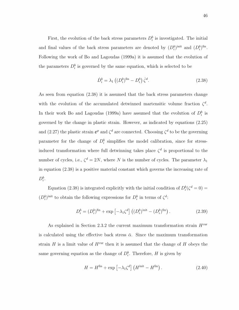
46

First, the evolution of the back stress parameters Dbi is investigated. The initial

and final values of the back stress parameters are denoted by (Dbi )

init and (Dbi )

fin.

Following the work of Bo and Lagoudas (1999a) it is assumed that the evolution of

the parameters Dbi is governed by the same equation, which is selected to be

Dbi = λ1

((Db

i )fin −Db

i

)ζd. (2.38)

As seen from equation (2.38) it is assumed that the back stress parameters change

with the evolution of the accumulated detwinned martensitic volume fraction ζd.

In their work Bo and Lagoudas (1999a) have assumed that the evolution of Dbi is

governed by the change in plastic strain. However, as indicated by equations (2.25)

and (2.27) the plastic strain εp and ζd are connected. Choosing ζd to be the governing

parameter for the change of Dbi simplifies the model calibration, since for stress-

induced transformation where full detwinning takes place ζd is proportional to the

number of cycles, i.e., ζd = 2N , where N is the number of cycles. The parameter λ1

in equation (2.38) is a positive material constant which governs the increasing rate of

Dbi .

Equation (2.38) is integrated explicitly with the initial condition of Dbi (ζ

d = 0) =

(Dbi )

init to obtain the following expressions for Dbi in terms of ζd:

Dbi = (Db

i )fin + exp

[−λ1ζd] (

(Dbi )

init − (Dbi )

fin). (2.39)

As explained in Section 2.3.2 the current maximum transformation strain Hcur

is calculated using the effective back stress α. Since the maximum transformation

strain H is a limit value of Hcur then it is assumed that the change of H obeys the

same governing equation as the change of Dbi . Therefore, H is given by

H = Hfin + exp[−λ1ζ

d] (H init −Hfin

). (2.40)

47

Similar evolution equations are proposed for the drag stress parameters Ddi . The

evolution of Ddi is described by

Ddi = (Dd

i )fin + exp [−λ2ζ ]

((Dd

i )init − (Dd

i )fin). (2.41)

where λ2 is a material parameter governing the evolution of Ddi . As seen from equa-

tion (2.41) the evolution of the drag stress parameters is governed by the total ac-

cumulated martensitic volume fraction ζ and not it’s detwinned portion ζd. This

is related to the fact that microstructural changes can be induced by cyclic self-

accommodating phase transformation (Bo and Lagoudas, 1999a). It should be noted

that for stress-induced phase transformation with large values of the applied stress

equations (2.38) and (2.41) are identical (if, of course, λ1 = λ2), since in this case

ζ = ζd.

Finally, the evolution of the material parameters Y , M0s and ρ∆s0 is considered.

The equations governing the change of these parameters are similar to equation (2.41):

Y = Y fin + exp [−λ3ζ ](Y init − Y fin

), (2.42)

M0s = (M0s)fin + exp [−λ4ζ ]((M0s)init − (M0s)fin

), (2.43)

ρ∆s0 = (ρ∆s0)fin + exp [−λ4ζ ]

((ρ∆s0)

init − (ρ∆s0)fin), (2.44)

where λ3, λ4 and λ5 are material parameters.

It should be noted that it may be very difficult to determine unique values for the

parameters λ1–λ5, because it is difficult to determine different values for the number

of cycles for each of the parameters to reach its final value. A reasonable argument

can be made that two unique values of the parameters λ1–λ5 can be determined. The

first value is for the parameter λ1 and it can be obtained by performing cyclic loading

during which the material undergoes stress-induced transformation. The second value

48

can be determined for the parameters λ2–λ5 by performing thermal cycling with no

applied stress. This separation of the parameters is explained by the different forms

of the evolution equations, in which λ1–λ5 enter. While the evolution equation for

the back stress parameters involves the accumulated detwinned martensitic volume

fraction ζd, the other evolution equations involve the accumulated total martensitic

volume fraction ζ . Therefore, in the case of self-accommodated thermally induced

transformation cycling the value of ζd is zero. Then, any change of the parameters

will be caused by the change in ζ , which will allow to determine the value of λ2–λ5.

Note, however, that in the case that only stress-induced transformation cycling results

are available, the above described approach is not applicable. One possible approach

in this case is to assume that the values of λ1–λ5 are all equal.

As discussed above, two sets of the material parameters need to be identified —

the initial set, characterizing the initial response of the annealed material and the

final set, characterizing the stable material response. Then, having identified these

two sets, the material parameters continuously change according to the evolution

equations. However, this situation poses a problem in identifying the initial and final

values of the parameters. Indeed, if the material parameters change continuously

during the identification of the first set, it is impossible to take into account the

change during the first cycle due to the nonlinearity introduced by that change.

This problem is addressed by keeping the value of the material parameters con-

stant during forward or reverse phase transformation. The parameters will be recalcu-

lated according to the evolution equations when a reversal of the phase transformation

occurs. Thus, the change in sign of the martensitic volume fraction rate ξ triggers the

change of the material parameters. Note, however, that the above procedure is valid

only for the material parameters. The plastic strain during cyclic loading is continu-

ously calculated during both forward and reverse phase transformation, according to

49

the evolution equation (2.25).

2.6. Modeling of Minor Hysteresis Loops

An important part of the thermomechanical constitutive modeling of SMAs is the

accounting for the minor hysteresis loops. In the context of the presented model a

major loop is characterized by a full transformation cycle with the martensitic volume

fraction ξ monotonically increasing from 0 to 1 and then monotonically decreasing

from 1 to 0. On the other hand, during a minor loop the martensitic volume frac-

tion ξ initial value is strictly greater than 0 and less than 1. To express the above

conditions in term of measurable physical quantities, consider a stress-induced phase

transformation. A major hysteresis loop occurs when the applied stress cycle has a

range greater than (σAf −σMf). For a stress path strictly inside (σAf −σMf ) a minor

loop occurs.2

The above described model in its current form indicates that the transformation

criterion is identical for both major and minor loops. This assumption has also been

made in the derivation of the majority of the models presented in the literature (Bo

and Lagoudas, 1999b; Boyd and Lagoudas, 1996; Tanaka, 1986). The ramification

of the above assumption is the prediction that a minor hysteresis loop is a part of a

major loop and, therefore, the incorrect prediction of the SMA response during minor

hysteresis loops. To illustrate the above discussion, minor hysteresis loops predicted

by the model are schematically shown inside a major loop in Figure 9. As seen from

Figure 9 during the minor loop the stress initially increases leading to partial forward

phase transformation. When unloading occurs the reverse phase transformation does

not start until the major hysteresis loop is reached. However, experimental results

2The definition of σAf and σMf is given in Section 1.2.2

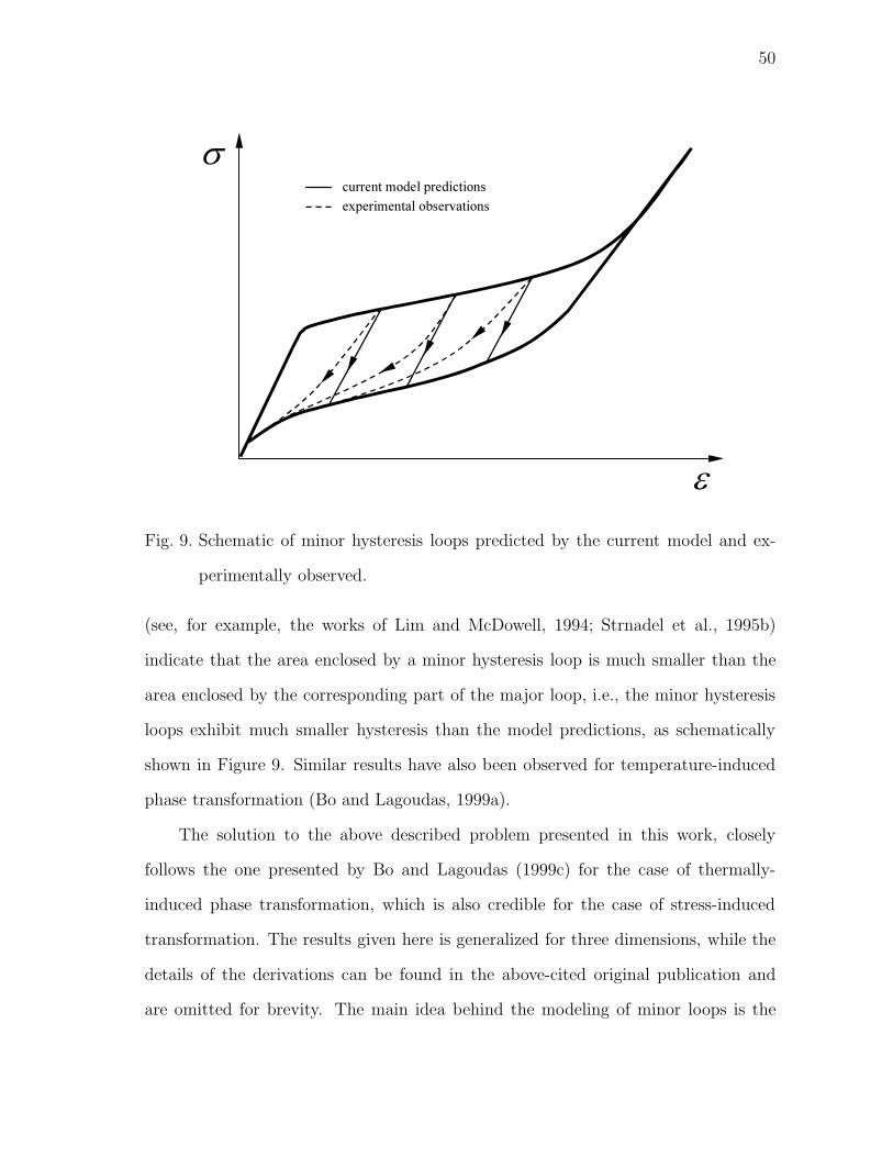
50

�

�

current model predictions

experimental observations

Fig. 9. Schematic of minor hysteresis loops predicted by the current model and ex-

perimentally observed.

(see, for example, the works of Lim and McDowell, 1994; Strnadel et al., 1995b)

indicate that the area enclosed by a minor hysteresis loop is much smaller than the

area enclosed by the corresponding part of the major loop, i.e., the minor hysteresis

loops exhibit much smaller hysteresis than the model predictions, as schematically

shown in Figure 9. Similar results have also been observed for temperature-induced

phase transformation (Bo and Lagoudas, 1999a).

The solution to the above described problem presented in this work, closely

follows the one presented by Bo and Lagoudas (1999c) for the case of thermally-

induced phase transformation, which is also credible for the case of stress-induced

transformation. The results given here is generalized for three dimensions, while the

details of the derivations can be found in the above-cited original publication and

are omitted for brevity. The main idea behind the modeling of minor loops is the

51

�

�

0132

0

Fig. 10. Definition of the order of minor loop branches.

modification of the transformation function, depending on whether the loading path

follows a major or a minor loop.

First, an order of each branch of the hysteresis curve is defined as follows: the

two branches of the major hysteresis loop are defined to be of order 0. The order of

a minor loop branch is defined to be the number of times the hysteresis curve has

reversed from a branch of the major loop (see Figure 10). For example, all first-order

branches are attached to the major loop, all second order are attached to a first-order

branch, etc.

Next, the thermodynamic driving force π conjugate to ξ for the nth order branch

of the hysteresis curve is introduced as πn. The transformation condition [cf. equa-

52

tion (2.18)] is modified as

Φ =

πn − Yn = 0, ξ > 0,

−πn − Yn = 0, ξ < 0,(2.45)

where Yn(ξ) is now the local energy dissipation per unit volume for the nth order

branch and is a function of ξ. πn is given by

πn =1

2σ : ∆S : σ + σ : ∆α(T − T0) + (σ + αn) : Λ + ηn

− ρ∆c

[T − T0 − T ln

(T

T0

)]+ ρ∆s0(T −M0s), (2.46)

where αn and ηn are the back and drag stresses for the nth order branch of the

hysteresis loop. The effect of the difference between αn and ηn and the corresponding

quantities for the major hysteresis loop is taken into account by introducing the

following function ∆ψn(ξ):

∆ψn(ξ) = [αn(ξ) − α0(ξ)] : Λ + ηn(ξ) − η0(ξ). (2.47)

Using equations (2.46) and (2.47) the following expression relating the thermody-

namic force for the nth branch πn and the corresponding one for the major hysteresis

curve π0 is derived:

πn = π0 + ∆ψn. (2.48)

Note that for a major loop Y0 is constant and ∆ψ0 = 0.

The evolution of the local energy dissipation Yn during a minor loop is proposed

as

Yn(ξ) = An

(1 − exp

[− γ

Cn|ξ − ξn

r |])

. (2.49)

In the above equation γ is a material constant, ξnr is the value of the martensitic

53

volume fraction at the reversal point and the parameter Cn is defined as

Cn = min {ξnr , 1 − ξn

r } . (2.50)

The choice of Cn as introduced by the above equation (2.50) is made to account

for the different rate of ξ at different transformation stages. The parameter An is

calculated from the following equation:

An =Yn−1(ξ

nr )

1 − exp[− γ

Cn|ξn−1

r − ξnr |] . (2.51)

Finally, it is assumed that the evolution of ∆ψn is similar to the evolution of Yn:

∆ψn(ξ) =

∆ψn(ξnr ) − Yn(ξ), ξ > 0,

∆ψn(ξnr ) + Yn(ξ), ξ < 0.

(2.52)

The initial condition for ∆ψn at ξ = ξnr is derived assuming that the phase transfor-

mation starts immediately at the point of reversal. It is given by

∆ψn(ξnr ) =

∆ψn−1(ξnr ) − Yn−1(ξ

nr ), ξ > 0,

∆ψn−1(ξnr ) + Yn−1(ξ

nr ), ξ < 0.

(2.53)

Finally, a few remarks on the implementation of the algorithm for minor loop

modeling are made. As indicated by Bo and Lagoudas (1999c), proper transforma-

tion history must be kept. The values of ξ and Yn for each reversal point must be

stored, as well as the value of the parameter Cn. However, some of the memory for

transformation history is wiped out by subsequent transformation. The wiping out

algorithm (Bo and Lagoudas, 1999c) is as follows:

• For the forward phase transformation if the values of ξ at previous forward-to-

reverse transformation reversal points are smaller than the current value of ξ

then the transformation history memory corresponding to those minor loops is

54

wiped out;

• For the reverse phase transformation if the values of ξ at previous reverse-to-

forward transformation reversal points are greater than the current value of ξ

then the transformation history memory corresponding to those minor loops is

wiped out;

This wiping out algorithm enforces the property that if the current nth order branch

goes beyond the previous reversal point ξn−1r of the (n − 1)st branch then the nth

order branch is reduced to (n− 2)nd order branch.

2.7. Estimation of Material Parameters

As a final step to characterizing the thermomechanical behavior in this section the de-

termination of the material parameters entering the model is discussed. Three groups

of material parameters are identified. First, the parameters which are necessary to

describe a stable transformation cycle are determined. In the context of the current

model the stable transformation cycle is defined as a thermomechanical loading cycle

during which no plastic strains are developed and the material parameters remain

constant. It should be mentioned that the above definition is realistic for the stable

material response. However, during the first cycles there is measurable plastic strain.

The effect of this plastic strain on the determination of the material parameters will

be discussed in a sequel. The second group includes the material parameters which

describe the behavior of SMA under cycling loading. These are the material parame-

ters governing the evolution of plastic strains as well as the evolution of the material

parameters from the first group. Finally, the third group encompasses the parameters

governing the SMA behavior during minor hysteresis loops. The material parameters

will be determined using uniaxial tests. Therefore, the one-dimensional reduction of

55

the model is given next.

2.7.1. One-Dimensional Reduction of the Model

During uniaxial loading the stress tensor has one non-zero component. Thus, the

components of the stress tensor are given by:

σ11 = σ = 0, σij = 0 for all other i, j. (2.54)

In the equation above σ is the applied uniaxial stress. The transformation and plastic

strain components are given by

εt11 = εt, εt

22 = εt33 = −1

2εt, εt

ij = 0 for all other i, j, (2.55)

εp11 = εp, εp

22 = εp33 = −1

2εp, εp

ij = 0 for all other i, j, (2.56)

where εt and εp are the uniaxial transformation and plastic strains. Assuming isotropic

elastic properties, the constitutive equations (2.9) in the one-dimensional form become

ε11 = ε = Sσ + α(T − T0) + εt + εp, (2.57)

where ε is the uniaxial total strain, α is the thermal expansion coefficient and S is

the elastic compliance given by

S =1

E, (2.58)

where E is the Young’s elastic modulus.

The evolution equations for the transformation and plastic strain become

εt = Λξ, (2.59)

εp = Λpζd. (2.60)

The uniaxial components of the transformation and plastic direction tensors are given

56

by

Λ = Λ11 =

Hcur σeff

|σeff| , ξ > 0,

εtmax

ξmax, ξ < 0,

(2.61)

Λp = Λp11 =

Cp1 exp

[− ζd

Cp2

]σeff

|σeff| , ξ > 0,

Cp1 exp

[− ζd

Cp2

]εtmax

ξmax, ξ < 0.

(2.62)

The uniaxial effective stress σeff is defined as

σeff = σ + α, (2.63)

where the back stress α is given by

α = −3

2

εt

|εt|Nb∑i=1

Dbi (H

curξ)(i). (2.64)

The expression for the drag stress η is the same as given by equation (2.30)

η = −Dd1 [− ln(1 − ξ)]

1m1 +Dd

2ξ. (2.65)

The transformation function is given by

Φ =

π − Y = 0, ξ > 0,

−π − Y = 0, ξ < 0,(2.66)

where the thermodynamic driving force π is given by

π =1

2σ2∆S + σ∆α(T − T0) + σeffΛ + η

− ρ∆c

[T − T0 − T ln

(t

T0

)]+ ρ∆s0(T −M0s) + Y. (2.67)

The quantity ∆S is the difference between the elastic compliances of the austenitic

and martensitic phases and is given by

∆S =1

EM− 1

EA(2.68)

57

and ∆α is the difference between the thermal expansion coefficients of the austenite

and martensite.

The uniaxial tangent stiffness and tangent thermal modulus are given by

L = E − χE2∂σΦ

χE∂σΦ − ∂ξΦ, (2.69)

Θ = E

[−χ Eα∂σΦ

χE∂σΦ − ∂ξΦ− α

], (2.70)

where the quantity χ is given by

χ = σ∆S + ∆α(T − T0) + Λ + sign(ξ)Hcur

HΛp. (2.71)

The derivatives of the transformation function with respect to stress, temperature

and the martensitic volume fraction are given by

∂σΦ = σ∆S + ∆α(T − T0) + Λ, (2.72)

∂T Φ = σ∆α + ρ∆c ln

(T

T0

), (2.73)

∂ξΦ = − 3

2

εt

|εt|ΛNb∑i=1

iHcurDbi (H

curξ)(i−1)

− 1

m1(1 − ξ)Dd

1 [− ln(1 − ξ)]1−m1

m1 +Dd2. (2.74)

The determination of the material parameters of all of the three groups is de-

scribed in detail in the following subsections. The tests which are necessary to be

performed will be discussed and a parametric study for selected material parameters

will be performed. The material parameters for NiTi reported by Bo et al. (1999)

and shown in Table I will be used during the parametric study.

58

Table I. Material parameters for NiTi SMA characterizing a stable transformation

cycle (Bo et al., 1999).

Physical constants

EA = 70.0 GPa αA = 11.0 × 10−6 K−1

EM = 30.0 GPa αM = 6.6 × 10−6 K−1

ρcA = 2.12 MJ/(m3K) ν = 0.33

ρcM = 2.12 MJ/(m3K)

Parameters characterizing the phase transformation

M0s = 311.0 K ρ∆s0 = −0.422 MJ/(m3K)

H = 0.069 Y = 6.0 MJ/m3

Db1 = 3.40 × 103 MPa Dd

1 = 8.0 MPa

Db2 = −2.23 × 105 MPa Dd

2 = 1.7 MPa

Db3 = 8.32 × 106 MPa m1 = 3.5

Db4 = −1.50 × 108 MPa

Db5 = 1.03 × 109 MPa

Minor loop parameter

γ = 3.0

59

2.7.2. Material Parameters for a Stable Transformation Cycle

This group of material parameters include the elastic compliance tensors of both

austenite martensite phases SA and SM , their thermal expansion coefficient tensors

αA and αM and specific heat cA and cM . The martensitic start temperature M0s,

maximum transformation strain H , the difference between the specific entropy per

unit volume ρ∆s0, the material parameter Y which provides a measure of the internal

dissipation during phase transformation and the parameters associated with the back

and drag stresses are also included in this group of parameters.

To determine the elastic compliance tensors SA and SM it is assumed that the

SMA material behaves isotropically at macroscale. This assumption is reasonable

because of the random orientation of the grains in a polycrystalline SMA. Therefore,

it is only necessary to find the Young’s elastic moduli and Poisson’s ratios EA, EM , νA

and νM of both phases. To determine the elastic constants a uniaxial pseudoelastic

test must be performed. The elastic stiffness EA is determined by calculating the

initial slope of the stress-strain curve for a uniaxial pseudoelastic test as shown in

Figure 11. The elastic stiffness of the martensite phase EM is given by the slope

of the stress-strain curve at the point of initial unloading (see Figure 11). It has

been generally assumed in the literature that the Poisson’s ratios of austenite and

martensite are equal and a typical value of νA = νM = 0.33 has been reported

(Lagoudas and Bo, 1999; Lagoudas et al., 1996).

The thermal expansion coefficient tensors αA and αM are fully represented by

two scalar constants αA and αM . These constants can be estimated by measuring the

slope of strain-temperature curve under constant stress at high temperature for the

austenitic phase and low temperature for the martensitic phase. The specific heat

constants cA and cM can be obtained from a calorimetric test. Note that these con-

60

�

�

AE

ME

Ms�

Area A

H

Fig. 11. Schematic of a uniaxial pseudoelastic test.

stants (αA, αM , cA, cM) are not needed to model stress-induced phase transformation

under constant temperature, but they become important when temperature changes.

The martensitic start temperature M0s can be obtained from a DSC test. De-

tailed description of the DSC setup and test is given by Bo et al. (1999). The maxi-

mum transformation strain H is obtained by performing a pseudoelastic uniaxial test.

Its value is estimated by extending the unloading part of the stress-strain curve using

the elastic stiffness of the martensitic phase EM , as shown in Figure 11.

As mentioned above, during the initial loading cycles observable plastic strain

can develop. One proposed way to separate the plastic strain from the transformation

strain is to subtract a portion of the residual plastic strain from the measured value of

the transformation strain. Since the plastic strain develops during both forward and

61

reverse transformation, the subtracted value must be adjusted to take into account the

plastic strain developed during the reverse phase transformation. As experimentally

observed and reflected in the evolution equation for the plastic strain, initially the

rate of accumulation of the plastic strain can be approximated by a linear function.

Therefore, it is reasonable to assume that the amount of the plastic strain developed

during the forward phase transformation is equal to one-half of the total residual

plastic strain after one cycle. Thus, in presence of plastic strains, the value of the

maximum transformation strain H is obtained by extending the unloading part of

the stress-strain curve and subtracting one-half of the total residual strain from the

obtained number.

The material parameter ρ∆s0 can also be obtained from the pseudoelastic stress-

strain curve, schematically shown in Figure 11. Using equations (2.66) and (2.67) for

the uniaxial isothermal stress loading the transformation function Φ at the onset of

phase transformation (ξ = 0) is given by

Φ =1

2(σMs)2∆S + σMsHcur + ρ∆s0(T −M0s). (2.75)

Then, using the transformation condition Φ = 0 the following expression for ρ∆s0 is

obtained

ρ∆s0 = −12(σMs)2∆S + σMsHcur

T −M0s. (2.76)

Note that the value of Hcur used in equation (2.76) should be calculated for the

corresponding value of stress, which in this case is equal to σMs. A slightly different

procedure for determination of M0s and ρ∆s0 is reported by Bo et al. (1999). In their

work, the quantity ρ∆s0 is calculated from the DSC test and is related to the latent

heat released during forward phase transformation and absorbed during reverse phase

transformation. The martensitic start temperature M0s is calculated in their work

62

0.00 0.01 0.02 0.03 0.04 0.05 0.06 0.07 0.08 0.09

Strain

0

100

200

300

400

500

600

Str

ess

, M

Pa

Value of ��s0

-0.6 MJ/m3K

-0.5 MJ/m3K

-0.4 MJ/m3K

-0.3 MJ/m3K

-0.2 MJ/m3K

Fig. 12. Effect of the parameter ρ∆s0 on the stress-strain response during forward

phase transformation.

using strain-temperature curve obtained during an isobaric experiment.

To demonstrate the effect of the value of ρ∆s0 on the stress-strain response,

loading cases with different numerical values of ρ∆s0 are simulated. The results of

the parametric study are shown in Figure 12 where only the loading part is shown. It

can be seen that with increasing magnitude of ρ∆s0 the value of stress for the onset

of the transformation also increases. Therefore, it can be seen that the parameter

ρ∆s0 is connected to the slope of the transformation line on the stress-temperature

phase diagram (see Figure 1).

The material parameter Y can also be calculated using a pseudoelastic stress-

strain curve. The value of Y is related to the total area A enclosed by the hysteresis

63

0.00 0.01 0.02 0.03 0.04 0.05 0.06 0.07 0.08 0.09

Strain

0

100

200

300

400

500

600

Str

ess

, M

Pa

Value of Y

2.0 MJ/m3

4.0 MJ/m3

6.0 MJ/m3

8.0 MJ/m3

Fig. 13. Effect of the parameter Y on the size of the hysteresis loop.

curve during a complete phase transformation as

A = 2Y. (2.77)

The effect of the parameter Y on the stress-strain response is shown in Figure 13.

The unloading parts of the stress-strain curves for different values of Y are shown in

the figure while the loading parts are the same for all values of Y . It can be seen

that with the increase of the value of Y the reverse phase transformation starts at

lower values of the applied stress. This, in effect, causes the increase of the area of

the hysteresis loop, as seen in Figure 13.

As mentioned earlier in Section 2.3.2 [cf. equation (2.24)] the effective back

stress is used to calculate the value of the current transformation strain Hcur. Thus,

64

an experimental result showing the dependance of Hcur on the value of the applied

stress σ is utilized to obtain the back stress parameters Dbi . To obtain this dependance

several isobaric tests with thermally-induced phase transformation must be performed

for different values of the applied stress. Each test gives one value of the current

maximum transformation strain Hcur corresponding to the value of the applied stress

(see Figure 14). Then, the back stress parameters Dbi are obtained using the condition

that the effective stress σeff at ξ = 1.0 vanishes. Therefore, a least-square fit of the

following equation is performed

σ =3

2

εt

|εt|Nb∑i=1

Dbi (H

cur)(i). (2.78)

After the value of Hcur reaches the value of the maximum transformation strain H it

is assumed that further increase of the stress does not yield further increase of Hcur.

After that point the value of Hcur is considered to be constant and equal to H .

Note that sometimes it is difficult to obtain experimental curves for σ vs. Hcur. In

case that this data is unavailable, a typical curve, similar to the one shown in Figure 14

can be used. The results shown in Figure 14 have been reported by Lagoudas and

Bo (1999) and similar results have also been observed by other researchers. Since for

a stress-induced martensite the values of stress are expected to be high enough to

induce complete detwinning of the martensitic variants, the errors introduced by this

approximation are expected to be relatively small. For temperature-induced phase

transformation, however, this experimental data is critical for the accuracy of the

model, since small variations in stress may cause large variations of Hcur.

To estimate the material parameters entering the expression for the drag stress

η the tangent stiffness during an isothermal uniaxial pseudoelastic test is used. As-

suming that all of the material parameters, except the drag stress parameters, are

known, the tangent stiffness L given by equation (2.69) becomes a function of the

65

0

20

40

60

80

100

120

140

160

180

200

0 0.1 0.2 0.3 0.4 0.5 0.6 0.7 0.8 0.9 1

App

lied

str

ess

, M

Pa

cur

H

H

Fig. 14. Normalized maximum transformation strain for thermally induced phase

transformation versus the applied stress: experimental data for NiTi

SMA (Lagoudas and Bo, 1999) and a polynomial least-square fit. A polyno-

mial of degree 5 is used.

drag stress parameters Dd1, D

d2 and m1 and the martensitic volume fraction ξ:

L(ξ;Dd1, D

d2, m1) = E − E2(σ∆S +Hcur)2

DEN,

(2.79)

where the denominator is given by

DEN = E(σ∆S +Hcur)2 +3

2(Hcur)2

Nb∑i=1

iDbi (H

curξ)(i−1)

+1

m1(1 − ξ)Dd

1 [− ln(1 − ξ)]1−m1

m1 −Dd2. (2.80)

The experimental values of the uniaxial tangent stiffness are obtained by per-

66

forming a pseudoelastic test. Thus, having obtained the experimental values of the

tangent stiffness, a least-square fit of equation (2.79) is performed to obtain the drag

stress parameters Dd1, D

d2 and m1. Note, that the internal parameter ξ cannot be

directly measured. Based on numerous numerical experiments performed using the

current model it has been found that it is reasonable to assume a linear relationship

between the rate of total strain and the rate of the martensitic volume fraction during

transformation.

To illustrate the effect of the drag stress parameters on the stress-strain results, a

parametric study for different values of Dd1 and Dd

2 has been performed. The loading

part of the pseudoelastic stress-strain curve for different values of Dd1 is shown in

Figure 15. It can be seen from the figure that the transformation hardening increases

with the increase of the value of Dd1. In addition, the value of Dd

1 has a very strong

effect on the initial transformation hardening. The effect of the parameter Dd2 on

the stress-strain results is shown in Figure 16. It can be seen that higher value of

the parameter Dd2 leads to smaller slope of the stress-strain curve. This parameter,

however, has very little effect on the initial transformation hardening. The effect of

Dd2 can be explained by comparing the expression for the drag stress in the current

model to the one given by Lagoudas et al. (1996) for a model with a polynomial

hardening function. If the parameter Dd1 is taken to be zero, then the parameter

Dd2 corresponds to the linear hardening parameter in the model by Lagoudas et al.

(1996). Therefore, it has the same effect for all values of ξ and its value equally affects

the slope of the stress-strain curve during the phase transformation.

2.7.3. Material Parameters for Cyclic Loading

This group of parameters includes the parameters Cp1 and Cp

2 , entering the expression

for Λp (2.62) and constants λ1–λ5, which determine the evolution of the material pa-

67

0.00 0.01 0.02 0.03 0.04 0.05 0.06 0.07 0.08 0.09

Strain

0

100

200

300

400

500

600

Str

ess

, M

Pa

Value of Dd 1

12.0 MPa

10.0 MPa

8.0 MPa

6.0 MPa

4.0 MPa

Fig. 15. Effect of the parameter Dd1 on the stress-strain response during forward phase

transformation.

rameters during cyclic loading. To understand the physical meaning of the constants

Cp1 and Cp

2 equation (2.60) can be integrated to find the following expression for εp

as a function of ζd:

εp = Cp1C

p2

(1 − exp

[− ζd

Cp2

]). (2.81)

As seen from equation (2.81) the product of Cp1 and Cp

2 gives the maximum (satu-

ration) value of the plastic strain. Further, recall that for stress-induced martensite

ζd = 2N . Therefore, Cp2 can be estimated by enforcing the condition that after a

given number of cycles the plastic strain approaches its maximum value, or more

68

0.00 0.01 0.02 0.03 0.04 0.05 0.06 0.07 0.08 0.09

Strain

0

100

200

300

400

500

600

Str

ess

, M

Pa

Value of Dd 2

1.0 MPa

3.0 MPa

5.0 MPa

Fig. 16. Effect of the parameter Dd2 on the stress-strain response during forward phase

transformation.

precisely, Cp2 can be found from the condition

exp

[−2Np

sat

Cp2

]= δ, (2.82)

where Npsat is the number of cycles to reach the saturation value of plastic strain and

δ is a small number.3

Next, parameters λ1, λ2 are considered. Only the estimation of λ1 is explained in

detail, due to the similarity between the equations containing this set of parameters.

It can be seen from equation (2.39) that λ1 determines the number of cycles N bsat

until Dbi reach their final values. Thus, it can be found using the following equation,

3Reasonable values for δ are in the range from 0.01 to 0.1

69

similar to equation (2.82):

exp[−2N b

satλ1

]= δ. (2.83)

The same procedure is used to find the parameter λ2.

2.7.4. Material Parameters for Minor Loop Modeling

Only one material parameter enters this last group. This is the constant γ, appearing

in equation (2.49) and dictating the size of the minor hysteresis loop. A smaller value

of γ leads to smaller area occupied by the minor loop, while larger value increases

the area. An experimental stress-strain curve with one minor loop is sufficient to

estimate the value of γ. A typical value of γ is in the range of 1 to 4. To illustrate

the effect of this parameter on the shape of the minor loop branches, the results for

different values of γ are shown in Figure 17.

70

0.00 0.01 0.02 0.03 0.04 0.05 0.06 0.07 0.08 0.09

Strain

0

100

200

300

400

500

600

Str

ess

, M

Pa

Value of �

1.0

2.0

4.0

Fig. 17. Effect of the parameter γ on the minor loop curvature. The minor loops

occur due to incomplete forward phase transformation.

71

CHAPTER III

NUMERICAL IMPLEMENTATION AND CORRELATION WITH

EXPERIMENTAL DATA FOR DENSE SMAS

In this chapter the numerical implementation of the thermomechanical constitutive

model for dense SMAs will be presented. The structure of the governing equations

of the SMA constitutive model is very similar to the structure of the equations char-

acterizing rate-independent plasticity in metals. Therefore, as shown by Qidwai and

Lagoudas (2000a) the numerical algorithms developed for integrating constitutive

equations characterizing plasticity can be successfully applied to integrate the equa-

tions for the SMAs. The approach taken in this work is to implement a return-

mapping for the dense SMA constitutive model, presented in Chapter II. The devel-

opment of the algorithm is based on the work of Qidwai and Lagoudas (2000a) with

special care taken to account for the development of plastic strains. The algorithm

used in the current work is an implementation of the closest point projection return

mapping algorithm.

The comparison of the model simulations with the available experimental re-

sults for dense SMAs undergoing cycling loading is also presented in this chapter.

The material parameters for the SMA are estimated using the data presented in the

literature.

3.1. Summary of the Dense SMA Constitutive Model Equations

For convenience the SMA constitutive equations presented in Chapter II are summa-

rized here. The strain ε is given by

ε = S : σ + α(T − T0) + εt + εp. (3.1)

72

The evolution equations for the transformation strain εt and the plastic strain εp are

given by

εt = Λξ, (3.2)

εp = Λpζd, (3.3)

where Λ and Λp are defined as

Λ =

32Hcur �eff′

σeff ξ > 0,

εtmax

ξmaxξ < 0,

(3.4)

Λp =

32Cp

1 exp[− ζd

Cp2

]�

eff′

σeff , ξ > 0,

Cp1 exp

[− ζd

Cp2

]εt

max

εtmax

, ξ < 0,(3.5)

and ζd is given by

ζd =

t∫0

|ξd(τ)|dτ. (3.6)

The effective stress σeff is defined in terms of the applied stress σ and the back stress

α as

σeff = σ + α. (3.7)

The transformation function Φ is defined as

Φ =

π − Y, ξ > 0,

−π − Y, ξ < 0.(3.8)

In the above equation π is the thermodynamic force conjugate to ξ and is given by

π =1

2σ : ∆S : σ + σ : ∆α(T − T0) + σ :

∂εt

∂ξ+ α :

∂εt

∂ξ+ η

− ρ∆c

[T − T0 − T ln

(T

T0

)]+ ρ∆s0(T −M0s) + Y. (3.9)

73

Expressions for the back stress α and the drag stress η are given in Section 2.3.4.

The evolution of the martensitic volume fraction ξ is constrained by the Kuhn–Tucker

conditions

ξ ≥ 0, Φ ≤ 0, Φξ = 0,

ξ ≤ 0, Φ ≤ 0, Φξ = 0.(3.10)

Thus the final system of algebraic and differential equations consists of equations (3.1)–

(3.3) which is constrained by equation (3.10).

3.2. Closest Point Projection Return Mapping Algorithm for SMA Constitutive

Model

To proceed with the solution of the above posed problem it is first assumed that

the strain and temperature histories ε(t) and T (t) are given. In addition, the initial

conditions for ξ, εt and εp are also known. The main idea of the return mapping

algorithms is to divide the problem into two parts. The first step is to obtain a

thermoelastic prediction, assuming that the transformation and plastic strains do

not change. During the second step, if the predicted thermoelastic state violates the

transformation condition, a transformation correction problem is solved to restore

consistency (Qidwai and Lagoudas, 2000a). During the transformation correction the

evolution equations for the transformation and plastic strains are discretized as

εtn+1 = εt

n + (ξn+1 − ξn) [βΛn+1 + (1 − β)Λn] , (3.11)

εpn+1 = εp

n + (ζdn+1 − ζd

n)[βΛp

n+1 + (1 − β)Λpn

], (3.12)

where β ∈ [0, 1] and subscript n indicates functional evaluation at time tn. Different

values of β will result in different integration algorithms. In this work β is chosen to be

equal to 1 which results in backward Euler integration rule. The resulting algorithm

74

is referred to as the closest point projection return mapping algorithm (Qidwai and

Lagoudas, 2000a). The stress-strain relation (3.1) for the case of β = 1 is also written

as

σn+1 = S−1n+1 :

(εn+1 − εt

n+1 − εpn+1 − αn+1(Tn+1 − T0)

). (3.13)

The main steps of the algorithm are described in detail in a sequel.

3.2.1. Thermoelastic Prediction

During the thermoelastic prediction step the following operations are performed:

εn+1 = εn + ∆εn+1, (3.14a)

Tn+1 = Tn + ∆Tn+1, (3.14b)

εt(0)n+1 = εt

n, (3.14c)

εp(0)n+1 = εp

n, (3.14d)

ξ(0)n+1 = ξn, (3.14e)

where ∆εn+1 and ∆Tn+1 are the (known) total strain and temperature increments

for the (n + 1)st time step. The superscript is introduced to indicate the current

iteration number, which for the case of (0) means evaluation of the quantities from

the previous time step. The value of the stress is obtained as

σ(0)n+1 = S−1

n :[εn+1 − ε

t(0)n+1 − ε

p(0)n+1 − αn(Tn+1 − T0)

]. (3.15)

The corresponding value of the transformation function Φ is evaluated as

Φ(0)n+1 = Φ(σ

(0)n+1, Tn+1, ξ

(0)n+1). (3.16)

At this point if the value of the transformation function satisfies the transfor-

mation criterion Φ(0)n+1 ≤ 0 than the thermoelastic trial state is the final, that is, no

75

phase transformation occurs at this time increment. However, if the transformation

criterion is violated, i.e., Φ(0)n+1 > 0 then a transformation correction is performed.

The transformation correction is performed by solving equations (3.11)–(3.13) with

initial guess given by equations (3.14), (3.15) and constrained by the Kuhn–Tucker

conditions (3.10). During the transformation correction the values of total strain εn+1

and temperature Tn+1 do not change. Only the values of the internal state variables

and the stress are updated.

3.2.2. Transformation Correction

To proceed with the transformation correction step, the following transformation and

plastic residuals are defined for the kth iteration as

Rt(k)n+1 = −ε

t(k)n+1 + εt

n + Λ(k)n+1(ξ

(k)n+1 − ξn) = 0, (3.17)

Rp(k)n+1 = −ε

p(k)n+1 + εp

n + Λp(k)n+1

∣∣∣ξd(k)n+1 − ξd

n

∣∣∣ = 0. (3.18)

The transformation (consistency) condition is given by

Φ(k)n+1 = Φ(σ

(k)n+1, Tn+1, ξ

(k)n+1) = 0. (3.19)

Equations (3.17)–(3.19) are solved using Newton–Raphson method. Keeping in

mind that during the transformation correction the total strain and temperature are

constant, the linearized forms of equations (3.17)–(3.19) using Taylor series expansion

become

Rt(k)n+1 − ∆ε

t(k)n+1 + ∆Λ

(k)n+1(ξ

(k)n+1 − ξn) + Λn+1∆ξ

(k)n+1 = 0, (3.20)

Rp(k)n+1 − ∆ε

p(k)n+1 + ∆Λ

p(k)n+1

∣∣∣ξd(k)n+1 − ξd

n

∣∣∣ + Λpn+1∆

∣∣∣ξd(k)n+1 − ξd

n

∣∣∣ = 0, (3.21)

Φ(k)n+1 + ∂�Φ

(k)n+1 : ∆σ

(k)n+1 + ∂ξΦ

(k)n+1∆ξ

(k)n+1 = 0. (3.22)

Next, the increment of the stress-strain constitutive relation (3.13) is taken which

76

yields

∆Sn+1 : σ(k)n+1 + Sn+1 : ∆σ

(k)n+1 = −∆αn+1(Tn+1 − T0) − ∆ε

t(k)n+1 − ∆ε

p(k)n+1. (3.23)

The increments of the elastic compliance tensor ∆Sn+1 and the thermal expansion

coefficient tensor ∆αn+1 are expressed using their evaluations [cf. equation (2.2)] in

terms of the increment of the martensitic volume fraction ξ as

∆Sn+1 = ∆S∆ξ(k)n+1, ∆αn+1 = ∆α∆ξ

(k)n+1. (3.24)

Using equations (3.24) and (3.23) the following expression for the increment of the

transformation strain ∆εt(k)n+1 is obtained:

∆εt(k)n+1 = −Sn+1 : ∆σ

(k)n+1 − ∆ε

p(k)n+1 −

[∆α(Tn+1 − T0) + ∆S : σ

(k)n+1

]∆ξ

(k)n+1. (3.25)

The increment of the transformation direction tensor ∆Λ(k)n+1 is given by

∆Λ(k)n+1 = ∂�Λ

(k)n+1 : ∆σ

(k)n+1. (3.26)

Equations (3.25) and (3.26) are substituted into equation (3.20) to obtain

[S

(k)n+1 + ∂�Λ

(k)n+1(ξ

(k)n+1 − ξn)

]: ∆σ

(k)n+1 =

−(R

t(k)n+1 + ∆ε

p(k)n+1 +

[∆α(Tn+1 − T0) + ∆S : σ

(k)n+1 + Λ

(k)n+1

]∆ξ

(k)n+1

). (3.27)

The increment of the plastic direction tensor ∆Λp(k)n+1 which enters equation (3.21)

is given by

∆Λp(k)n+1 = ∂�Λ

p(k)n+1 : ∆σ

(k)n+1 + ∂ξΛ

p(k)n+1 : ∆ξ

(k)n+1, (3.28)

77

while the quantity ∆∣∣∣ξd(k)

n+1 − ξdn

∣∣∣ is given by

∆∣∣∣ξd(k)

n+1 − ξdn

∣∣∣ = ∆

∣∣∣∣∣(Hcurξ

H

)(k)

n+1

−(Hcurξ

H

)n

∣∣∣∣∣= sign

((Hcurξ

H

)(k)

n+1

−(Hcurξ

H

)n

)Hcur

H∆ξ

(k)n+1. (3.29)

Thus, using equations (3.28), (3.29) expression (3.21) becomes

Rp(k)n+1 − ∆ε

p(k)n+1 + ∂�R

p(k)n+1 : ∆σ

(k)n+1 + ∂ξR

p(k)n+1 : ∆ξ

(k)n+1 = 0, (3.30)

where the quantities ∂�Rp(k)n+1 and ∂ξR

p(k)n+1 are defined as

∂�Rp(k)n+1 ≡

∣∣∣ξd(k)n+1 − ξd

n

∣∣∣ ∂�Λp(k)n+1, (3.31)

∂ξRp(k)n+1 ≡

∣∣∣ξd(k)n+1 − ξd

n

∣∣∣ ∂ξΛp(k)n+1 +

Hcur

Hsign

(ξ

d(k)n+1 − ξd

n

)Λ

p(k)n+1. (3.32)

The increment of the plastic strain ∆εp(k)n+1 is expressed using equation (3.30) and

substituted into equation (3.27) to obtain

[S

(k)n+1 + ∂�Λ

(k)n+1(ξ

(k)n+1 − ξn) + ∂�R

p(k)n+1

]: ∆σ

(k)n+1 =

−(R

t(k)n+1 + R

p(k)n+1 +

[∆α(Tn+1 − T0) + ∆S : σ

(k)n+1 + Λ

(k)n+1 + ∂ξR

p(k)n+1

]∆ξ

(k)n+1

).

(3.33)

To simplify further derivations the following tensorial quantities are defined

Ξ(k)n+1 ≡

[S

(k)n+1 + ∂�Λ

(k)n+1(ξ

(k)n+1 − ξn) + ∂�R

p(k)n+1

]−1

, (3.34)

χ(k)n+1 ≡ ∆α(Tn+1 − T0) + ∆S : σ

(k)n+1 + Λ

(k)n+1 + ∂ξR

p(k)n+1, (3.35)

which leads to the following expression for the increment of stress ∆σ(k)n+1:

∆σ(k)n+1 = −Ξ

(k)n+1 :

[R

t(k)n+1 + R

p(k)n+1 + χ

(k)n+1∆ξ

(k)n+1

]. (3.36)

78

Thus, the only unknown is the increment of the martensitic volume fraction

∆ξ(k)n+1. The consistency condition (3.22) together with equation (3.36) is used to find

∆ξ(k)n+1 =

∂�Φ(k)n+1 : Ξ

(k)n+1 :

[R

t(k)n+1 + R

p(k)n+1

]− Φ

(k)n+1

∂ξΦ(k)n+1 − ∂�Φ

(k)n+1 : Ξ

(k)n+1 : χ

(k)n+1

. (3.37)

Once ∆ξ(k)n+1 is found from equation (3.37) it is used to calculate the increment

of stress using equation (3.36). Then the increments of plastic and transformation

strain are found using equations (3.30) and (3.25).

Finally the expressions for ∂�Φ(k)n+1, ∂ξΦ

(k)n+1, ∂�Λ

(k)n+1, ∂�Λ

p(k)n+1 and ∂ξΛ

p(k)n+1 which

are used in the algorithm are derived. The derivative of the transformation function

with respect to stress can be obtained by differentiating equation (3.8). It follows

that

∂�Φ(k)n+1 =

∂�π(k)n+1, ξ > 0,

−∂�π(k)n+1, ξ < 0.

(3.38)

Using equation (3.9) the derivative of the thermodynamic driving force π with respect

to stress is given by

∂�π(k)n+1 = ∆α(Tn+1 − T0) + ∆S : σ

(k)n+1 + Λ

(k)n+1. (3.39)

Similarly the derivative of the transformation function with respect to the martensitic

volume fraction is

∂ξΦ(k)n+1 =

∂ξα(k)n+1 : Λ

(k)n+1 + ∂ξη

(k)n+1, ξ > 0,

−∂ξα(k)n+1 : Λ

(k)n+1 − ∂ξη

(k)n+1, ξ < 0.

(3.40)

The quantities ∂ξα(k)n+1 and ∂ξη

(k)n+1 are calculated using the expressions for α and η

[cf. equations (2.29), (2.30)].

Using equation (3.4) the derivative of the transformation direction tensor with

respect to stress ∂�Λ(k)n+1 is evaluated for the case of forward phase transformation

79

(ξ > 0) as

∂�Λ(k)n+1 =

3

2∂�H

cur ⊗ σeff′

σeff+

3

2Hcur∂�

[σeff′

σeff

], (3.41)

where the iteration counter k and the time step number (n+1) have been omitted for

perspicuity. The corresponding derivative for the case of reverse phase transformation

is equal to zero. To calculate the derivative of the current maximum transformation

strain with respect to stress ∂�Hcur recall equation (2.24). Differentiating both sides

of equation (2.24) result in

∂�σ = ∂� α|ξ=1 = ∂Hcurα|ξ=1 ∂�Hcur. (3.42)

Therefore, ∂�Hcur is given by

∂�Hcur =

∂�σ

∂Hcurα|ξ=1

. (3.43)

After performing standard calculations the expression for ∂�σ is found to be

∂�σ =3

2

σ′

σ. (3.44)

To calculate the second term of equation (3.41) the quantity ∂�

[�

eff′

σeff

]must be found.

Again, performing standard operations the following expression is derived:

∂�

[σeff′

σeff

]=

1

σeff

[I − 1

31 ⊗ 1 − 3

2

σeff′

σeff⊗ σeff′

σeff

]. (3.45)

The quantity I is the most general rank four symmetric identity tensor whose com-

ponents are given by

Iijk� =1

2(δikδj� + δi�δjk) . (3.46)

Similarly, the derivative of the plastic direction tensor with respect to stress

80

∂�Λp(k)n+1 for the case of forward phase transformation is calculated as

∂�Λp(k)n+1 =

3

2Cp

1 exp

[− ζd

Cp2

]∂�

[σeff′

σeff

], (3.47)

while the corresponding derivative for the case of reverse phase transformation is

again equal to zero. The derivative of Λp(k)n+1 with respect to ξ is given by

∂ξΛp(k)n+1 =

−32

Cp1

Cp2

exp[− ζd

Cp2

]Hcur

H�

eff′

σeff , ξ > 0,

Cp1

Cp2

exp[− ζd

Cp2

]Hcur

Hεt

max

εtmax

, ξ < 0.(3.48)

3.2.3. Consistent Tangent Stiffness and Thermal Moduli Tensors

The solution of the constitutive equations for the SMA involves calculating the stress

increment for a given strain and temperature increment at each time step. This

procedure makes use of the tangent stiffness tensor and the thermal tangent moduli

tensor, appearing in the linearized problem. An example of such a situation is a

displacement-based finite element method formulation which uses Newton’s method

to solve the resulting non-linear equations. As mentioned by Qidwai and Lagoudas

(2000a) the tangent tensors used by the global Newton’s method must be obtained in

a manner consistent with the integration algorithm. The use of the continuum tan-

gent tensors, derived in Section 2.4 would lead to a loss of the quadratic convergence

of Newton’s iterative method (Simo and Taylor, 1985). Therefore, in this section the

consistent tangent moduli tensors which are calculated at the end of the transforma-

tion correction iterative procedure and are passed to the global Newton’s method are

derived.

81

The total differential of the stress-strain relation (3.13) result in

∆S : σn+1dξn+1 + Sn+1 : dσn+1 = dεn+1 − dεtn+1 − dεp

n+1

− αn+1dTn+1 − ∆α(Tn+1 − T0)dξn+1. (3.49)

The differential of the flow rules for the transformation and plastic strains [cf. equa-

tions (3.11), (3.12)] result in

dεtn+1 = Λn+1dξn+1 + (ξn+1 − ξn)∂�Λn+1 : dσn+1, (3.50)

dεpn+1 = ∂�R

pn+1 : dσn+1 + ∂ξR

pn+1dξn+1, (3.51)

where the quantities ∂�Rpn+1 and ∂ξR

pn+1 are defined by equations (3.31), (3.32). The

substitution of equations (3.50) and (3.51) into equation (3.49) eventually leads to

dσ = Ξn+1 :[dε − αn+1dTn+1 − χn+1dξn+1

], (3.52)

where Ξn+1 and χn+1 are defined by equations (3.34), (3.35). Next, the consistency

condition is written in the following form:

dΦn+1 = ∂�Φn+1 : dσn+1 + ∂ξΦn+1dξn+1 + ∂T Φn+1dTn+1 = 0. (3.53)

Equation (3.52) together with equation (3.53) give the following expression for dξn+1:

dξn+1 =∂�Φn+1 : Ξn+1 : [dε − αn+1dTn+1] + ∂T Φn+1dTn+1

∂�Φ : Ξn+1 : χn+1 − ∂ξΦ. (3.54)

Upon substituting equation (3.54) into equation (3.52) the following expression for

dσn+1 is obtained:

dσn+1 =

[Ξn+1 − Ξn+1 : χn+1 ⊗ ∂�Φ : Ξn+1

∂�Φ : Ξn+1 : χn+1 − ∂ξΦ

]: dεn+1

+ Ξn+1 :

[χn+1

∂�Φ : Ξn+1 : αn+1 − ∂T Φn+1

∂�Φ : Ξn+1 : χn+1 − ∂ξΦ− αn+1

]dTn+1. (3.55)

82

The consistent tangent stiffness tensor Ln+1 and the consistent tangent thermal

moduli tensor Θn+1 are defined as

Ln+1 ≡ dσn+1

dεn+1= Ξn+1 − Ξn+1 : χn+1 ⊗ ∂�Φ : Ξn+1

∂�Φ : Ξn+1 : χn+1 − ∂ξΦ, (3.56)

Θn+1 ≡ dσn+1

dTn+1

= Ξn+1 :

[χn+1

∂�Φ : Ξn+1 : αn+1 − ∂T Φn+1

∂�Φ : Ξn+1 : χn+1 − ∂ξΦ− αn+1

]. (3.57)

3.2.4. Update of the Material Parameters

As explained in Section 2.5 the material parameters are updated only at the points of

reversal of the phase transformation. To update them, the evolution equations (2.41)–

(2.44) are utilized. These equations require knowledge of two parameters, which are

the accumulated martensitic volume fraction ζ and accumulated detwinned marten-

sitic volume fraction ζd. Therefore, these variables must be made available and must

be updated at each increment. To accomplish this, after the convergence of the return

mapping iterative procedure, the values of ζ and ζd are calculated using their val-

ues from the previous increment and the newly found values of the increment of the

martensitic volume fraction ∆ξn+1 and the current maximum transformation strain

Hcurn+1.

3.2.5. Summary of the Numerical Algorithm for Dense SMA Constitutive Model

A summary of all steps of the numerical algorithm for the fully dense SMA are

presented in Table II. The notation used in the summary is the same as the one used

throughout this section, i.e., the current step number is n + 1 and all the quantities

from the previous nth step are known.

83

Table II. Summary of the closest point projection numerical algorithm for dense SMA

constitutive model.

1. Let k = 0, εn+1 = εn + ∆εn+1, Tn+1 = Tn + ∆Tn+1, εt(0)n+1 = εt

n, εp(0)n+1 = εp

n,

ξ(0)n+1 = ξn, S

(0)n+1 = Sn, α

(0)n+1 = αn.

2. Calculate σ(k)n+1, Φ

(k)n+1, R

t(k)n+1, R

p(k)n+1:

σ(k)n+1 = S

(k)−1n+1 :

[εn+1 − ε

t(k)n+1 − ε

p(k)n+1 − α

(k)n+1(Tn+1 − T0)

]Φ

(k)n+1 = Φ(σ

(k)n+1, Tn+1, ξ

(k)n+1)

Rt(k)n+1 = −ε

t(k)n+1 + εt

n + Λ(k)n+1(ξ

(k)n+1 − ξn)

Rp(k)n+1 = −ε

p(k)n+1 + εp

n + Λp(k)n+1

∣∣∣ξd(k)n+1 − ξd

n

∣∣∣If Φ

(k)n+1 < 0 OR

∣∣∣∆ξ(k)n+1

∣∣∣ < TOL1 then go to 8.

3. Check for reversal of the loading direction.

If the loading direction is reversed update the material parameters.

4. Calculate Ξ(k)n+1 and χ

(k)n+1:

Ξ(k)n+1 =

[S

(k)n+1 + ∂�Λ

(k)n+1(ξ

(k)n+1 − ξn) + ∂�R

p(k)n+1

]−1

χ(k)n+1 = ∆α(Tn+1 − T0) + ∆S : σ

(k)n+1 + Λ

(k)n+1 + ∂ξR

p(k)n+1

5. Calculate the increments of the martensitic volume fraction ∆ξ(k)n+1,

stress ∆σ(k)n+1, transformation strain ∆ε

t(k)n+1 and plastic strain ∆ε

p(k)n+1:

∆ξ(k)n+1 =

∂�Φ(k)n+1 : Ξ

(k)n+1 :

[R

t(k)n+1 + R

p(k)n+1

]− Φ

(k)n+1

∂ξΦ(k)n+1 − ∂�Φ

(k)n+1 : Ξ

(k)n+1 : χ

(k)n+1

∆σ(k)n+1 = −Ξ

(k)n+1 :

[R

t(k)n+1 + R

p(k)n+1 + χ

(k)n+1∆ξ

(k)n+1

]∆ε

p(k)n+1 = −R

p(k)n+1 − ∂�R

p(k)n+1 : ∆σ

(k)n+1 − ∂ξR

p(k)n+1 : ∆ξ

(k)n+1

∆εt(k)n+1 = −Sn+1 : ∆σ

(k)n+1 − ∆ε

p(k)n+1 −

[∆α(Tn+1 − T0) + ∆S : σ

(k)n+1

]∆ξ

(k)n+1

84

Table II. Continued.

6. Update martensitic volume fraction, transformation and plastic strains,

elastic compliance tensor and thermal expansion coefficient tensor:

ξ(k+1)n+1 = ξ

(k)n+1 + ∆ξ

(k)n+1

εt(k+1)n+1 = ε

t(k)n+1 + ∆ε

t(k)n+1

εp(k+1)n+1 = ε

p(k)n+1 + ∆ε

p(k)n+1

S(k+1)n+1 = SA + ξ

(k+1)n+1 ∆S

α(k+1)n+1 = αA + ξ

(k+1)n+1 ∆α

7. Set iteration counter k = k + 1. Go to 2.

8. Calculate consistent tangent stiffness tensor Ln+1 and

thermal moduli tensor Θn+1:

Ln+1 = Ξn+1 − Ξn+1 : χn+1 ⊗ ∂�Φ : Ξn+1

∂�Φ : Ξn+1 : χn+1 − ∂ξΦ

Θn+1 = Ξn+1 :

[χn+1

∂�Φ : Ξn+1 : αn+1 − ∂T Φn+1

∂�Φ : Ξn+1 : χn+1 − ∂ξΦ− αn+1

]9. Update ζn+1 and ζd

n+1:

ζn+1 = ζn + |∆ξn+1|ζdn+1 = ζd

n +Hcur

n+1

H|∆ξn+1|

The numerical algorithm presented in this chapter is implemented as a user ma-

terial subroutine (UMAT) which is used by the FEM package ABAQUS (HKS, 1997).

All of the essential steps of finite element analysis — mesh generation, assembly of the

equations and their solution, the global Newton’s method to resolve the nonlinearity,

etc. — are handled by ABAQUS. When the analyses involve an SMA material, the

UMAT is called by ABAQUS. The internal state variables (ξ, εt, εp, etc.) for each

integration point are stored in a designated array and updated after each call to the

subroutine.

85

3.3. Test Cases for Numerical Implementation

To test the numerical implementation of the model for dense SMAs and to demon-

strate the capabilities of the model, different boundary-value problems (BVPs) are

presented in this section. First, a uniaxial isothermal pseudoelastic case is presented.

The second BVP represents a uniaxial thermally-induced transformation under con-

stant stress. Finally, the third BVP involves a torsion-compression loading of a cylin-

drical SMA specimen. The material parameters for all of the three cases are the ones

given by Bo et al. (1999) and are presented in Table I.

3.3.1. Uniaxial Isothermal Pseudoelastic Loading

The schematic of the BVP for this loading case is shown in Figure 18. The domain is

chosen to be a unit cube (1×1×1 m). Since the stress is constant in the whole domain

during the loading, a finite element mesh of only one linear element is chosen. Initially,

the material is in stress-free state. During the first step of the loading, the stress is

increased to 600 MPa which results in stress-induced phase transformation. During

the unloading step a reverse phase transformation occurs. The stress-strain response

of the material for this case is shown in Figure 19 for two different temperatures:

70�C and 80�C.

In the case of loading at T = 70�C it can be seen that the forward phase transfor-

mation starts at the value of applied stress approximately equal to 210 MPA and the

transformation is completed at 510 MPA. At the point of completion of the forward

transformation the value of the transformation strain is equal to the value of the maxi-

mum transformation strain H = 0.069. The onset of the reverse phase transformation

is at 350 MPa and the transformation is completed at 40 MPa. During the reverse

phase transformation, the transformation strain changes from its maximum value to

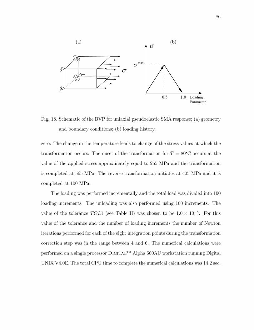
86

(a)

Loading

Parameter

1.0

max

�

0.5

(b)

�

�

Fig. 18. Schematic of the BVP for uniaxial pseudoelastic SMA response; (a) geometry

and boundary conditions; (b) loading history.

zero. The change in the temperature leads to change of the stress values at which the

transformation occurs. The onset of the transformation for T = 80�C occurs at the

value of the applied stress approximately equal to 265 MPa and the transformation

is completed at 565 MPa. The reverse transformation initiates at 405 MPa and it is

completed at 100 MPa.

The loading was performed incrementally and the total load was divided into 100

loading increments. The unloading was also performed using 100 increments. The

value of the tolerance TOL1 (see Table II) was chosen to be 1.0 × 10−8. For this

value of the tolerance and the number of loading increments the number of Newton

iterations performed for each of the eight integration points during the transformation

correction step was in the range between 4 and 6. The numerical calculations were

performed on a single processor Digitaltm Alpha 600AU workstation running Digital

UNIX V4.0E. The total CPU time to complete the numerical calculations was 14.2 sec.

87

0.00 0.01 0.02 0.03 0.04 0.05 0.06 0.07 0.08 0.09

Strain

0

100

200

300

400

500

600

Str

ess

, M

Pa

Temperature

70ºC

80ºC

Fig. 19. Pseudoelastic uniaxial SMA response.

3.3.2. Uniaxial Isobaric Thermally-Induced Transformation

Thus BVP describes a thermal cycle of a uniaxial SMA specimen under constant

applied stress. The schematic of the BVP and the loading history are shown in Fig-

ure 20. Initially the material is isothermally loaded to a given stress level which is

then kept constant. The first loading step involves cooling of the SMA from the

initial temperature of 100�C to the final temperature of 0�C. During this loading

step a forward phase transformation occurs and the transformation strain develops.

The final value of the transformation strain after the completion of the phase trans-

formation is dictated by the level of the applied stress and is equal to the current

maximum transformation strain Hcur. To illustrate the dependance of Hcur on the

applied stress, cases with different values of the applied stress are performed. During

88

the second loading step the material is heated back to 100�C and the transformation

strain is recovered.

(a)

Loading

Parameter

T

1.0

max

T

0.5

(b)

const� �

minT

Fig. 20. Schematic of the BVP for uniaxial isobaric thermally-induced transformation;

(a) geometry and boundary conditions; (b) loading history.

The results for the loading cases are shown in Figure 21. Two different effects of

the level of the applied stress on the results are observed. First, as mentioned above,

the maximum transformation strain during the phase transformation increases with

the increase of the value of the applied stress. The second effect is the shift of the

initial transformation temperature: the transformation starts at higher temperature

for higher value of the applied stress. This shift of the transformation temperatures

can be explained by recalling the expression for the transformation function, given

by equations (3.8) and (3.9). As seen from equation (3.9) with higher value of the

applied stress the transformation criterion will be satisfied for higher temperature.

3.3.3. Torsion-Compression Loading

While both of the previous loading cases were uniaxial, the model is also capable

of handling three-dimensional loading cases. To demonstrate such loading cases, the

89

270 280 290 300 310 320 330 340 350 360 370 380

Temperature, K

0.00

0.01

0.02

0.03

0.04

0.05

0.06

0.07

0.08

Strain

Applied Stress

200 MPa

120 MPa

80 MPa

30 MPa

Fig. 21. Strain versus temperature for different values of the applied stress.

response of a cylindrical SMA bar subjected to combined torion-compression and

torsion followed by compressive loading is modeled. The schematic of the BVPs is

shown in Figure 22. The specimen is chosen to have a diameter of 13 mm and length of

35 mm.1 The domain is discretized using eight-node quadratic axisymmetric elements

with a twist degree of freedom (elements CGAX8, for details see HKS, 1997). Since

there is no stress variation in the axial direction, only one layer of elements is used

in that direction with a length of 1.75 mm, while 5 elements are used in the radial

direction, as shown in Figure 22c. The maximum value of the applied rotation (see

Figure 22) is taken to be θmax = 0.02 rad (≈ 1.15�), which corresponds to 11.4 rad/m

1The dimensions are chosen to correspond to the dimensions of a porous SMA barwhich will be presented in Section 5.2.2

90

rotation (≈ 1.8 full revolutions per meter length), while the maximum value of the

displacement in the axial direction is taken to be umaxz = −0.125 mm, corresponding

to axial compressive strain of εzz = 0.071. Both compression and rotation boundary

conditions are applied on the top surface of the specimen, while the bottom surface

is held fixed in the z− and θ− directions. Traction-free boundary condition in the

radial direction is applied. The numerical simulations are performed at a temperature

of 60�C.

35 mm

13 mm

(a)

Loading

Parameter

�

zu

1

max

zu

max

�

(b)

0z

u u�

� �

0r

u �

Applied rotation

and compression

(c)

axis of

symmetry

0.5

simultaneous

sequential

z

r

Fig. 22. Schematic of the BVP for multiaxial loading of an SMA bar; (a) geometry;

(b) loading history; (c) finite element mesh and boundary conditions.

First the results for the sequential torsion-compression loading are presented.

During the first loading step when the bar is subjected to torsion a nonhomogeneous

stress state is created. As the stress increases the critical stress for the onset of

the phase transformation is first reached at the outer surface of the bar. The phase

transformation front then propagates towards the center of the bar. To illustrate this,

the contour plot of the martensitic volume fraction for the cross-section of the bar at

the end of the torsional loading (when the value of the loading parameter is equal to

91

Axis of symmetry

Element used to plot stresses

� VALUE

+7.20E-03

+6.93E-02

+1.31E-01

+1.94E-01

+2.56E-01

+3.18E-01

+3.80E-01

+4.42E-01

+5.04E-01

+5.66E-01

+6.28E-01

+6.90E-01

+7.52E-01

+8.15E-01

Fig. 23. Contour plot of the martensitic volume fraction in the SMA bar at the end

of the torsional loading.

0.5) is shown in Figure 23. It can be seen that the lines of constant value of ξ form

concentric circles.

The history of the axial and shear stress components during both loading steps is

shown in Figure 24. The average values of these quantities are shown for the element

indicated in Figure 24. During the initial torsional loading the shear stress linearly

increases until a critical value is reached. At this point (at the value of the loading

parameter of ≈ 0.1) the phase transformation initiates. During the first loading

92

0.00 0.25 0.50 0.75 1.00

Loading parameter

-900

-750

-600

-450

-300

-150

0

Str

ess

, M

Pa

�z�

�zz

Fig. 24. History of the axial and shear stress components during sequential torsion-

compression loading.

step the axial stress component remains zero. During the second loading step the

phase transformation continues until it is fully completed (at the value of the loading

parameter of ≈ 0.9). The axial stress increases while the shear stress is partially

relaxed. After the completion of the phase transformation the material is fully in the

martensitic phase and behaves linearly.

To explain the partial relaxation of the shear stress during the compressive axial

loading, consider the shear and axial components of the transformation strain, shown

in Figure 25. It is seen that during the second loading step, when a compressive

loading is applied, the shear component of the transformation strain continues to

increase. This is caused by the choice of the functional form of the transformation

direction tensor Λ, given by equation (2.22). Since the shear component of the

stress is non-zero, the shear component of the transformation strain keeps developing

during the second loading step, albeit with a smaller rate. On the other hand, since

the applied rotation and, therefore, the total strain, is kept constant during the

93

0.00 0.25 0.50 0.75 1.00

Loading parameter

-0.05

-0.04

-0.03

-0.02

-0.01

0.00

Tra

nsfo

rmati

on

str

ain

�t

z�

�t

zz

Fig. 25. History of the axial and shear transformation strain components during se-

quential torsion-compression loading.

compressive loading, the shear component of the stress decreases according to the

constitutive equation (2.9).

The history of the axial and shear stress components for the simultaneous torsion-

compression loading case are presented in Figure 26. The results for this loading

case resemble superposition of the results under compression and torsion applied

independently. The stresses increase linearly until a critical value is reached and

transformation initiates (the value of the loading parameter approximately equal to

0.05). Then the transformation proceeds until the material is fully transformed at the

value of the loading parameter approximately equal to 0.9. After the transformation

is completed, the response of the material is again linear with the elastic properties

of the martensite.

94

0.00 0.25 0.50 0.75 1.00

Loading parameter

-400

-300

-200

-100

0

Str

ess

, M

Pa

�z�

�zz

Fig. 26. History of the axial and shear stress components during simultaneous torsion-

compression loading.

3.4. Correlation with Experimental Data

The experimental results for NiTi undergoing cyclic loading will be simulated in

this section. The experimental data for one of the NiTi alloys reported by Strnadel

et al. (1995b) and presented in Section 2.1 will be used. Two types of tests were

performed by Strnadel et al. (1995b): the first type involved cycling, during which

the material is loaded to the same value of strain during each cycle and the second

type involved cycling performed to a given constant value of stress. Both types of tests

have been performed at a temperature higher than the austenitic finish temperature

A0f . The data for alloy “A”, which refers to one of the six tested alloys in the

original publication (Strnadel et al., 1995b) and has the composition Ti-50.9at%Ni.

The experimental results for alloys “A” for loading cases are shown on the top of

Figure 8. Based on the dimensions of the specimen and the reported elongation the

maximum value of strain during the first cycling test is estimated to be equal to

εmax = 0.04. The maximum value of the stress during the second test is reported to

95

be σmax = 550MPa. Twenty loading-unloading cycles with a constant maximum value

of strain have been performed, while the number of cycles with a constant maximum

value of strain is 50.

First the material parameters for the alloy are determined based on the exper-

imental graphs and reported data. The procedure described in Section 2.6 is used.

The obtained parameters are given in Table III. It should be mentioned that there

is no data on the dependance of the current maximum transformation strain Hcur on

the value of the applied stress. Therefore, the data shown in Figure 14 is used to

obtain the back stress coefficients Dbi . The coefficients are obtained for the value of

the maximum transformation strain for high values of stress H = 0.038) as reported

by Strnadel et al. (1995b). A polynomial of degree 5 is used in the expression for

the back stress. Based on the experimental results the back stress parameters are

assumed to be the same for both the initial and the final state of the material and

are given by Db1 = 6.18 × 103 MPa, Db

2 = −7.37 × 105 MPa, Db3 = 4.98 × 107 MPa,

Db4 = −1.63 × 109 MPa and Db

5 = 2.03 × 1010 MPa.

The initial set of material parameters has been determined using the initial trans-

formation cycle for the case of loading to a maximum value of stress, while the final

set has been determined from the stress-strain response after 50 cycles (see Figure 8).

In addition, as seen from Table III the parameters λ1 and λ2 have been selected to

be the same. Their value has been determined such that the material parameters

reach their saturation values after 50 cycles. As seen from Table III, not all of the

parameters change their values during the transformation cycling. Based on the ex-

perimental results the maximum transformation strain is assumed to be constant.

Only the initial value of the martensitic start temperature is reported in the work

by Strnadel et al. (1995b) and thus here it is also assumed to remain constant. Four

of the parameters — αA, αM , cA, cM — are taken from the work of Lagoudas and

96

Table III. Material parameters for NiTi alloy “A”.

Parameters remaining constant during cyclic loading

EA = 46.0 GPa αA = 11.0 × 10−6 K−1

EM = 25.0 GPa αM = 6.0 × 10−6 K−1

ν = 0.33 ρcA = 2.12 MJ/(m3K)

m1 = 3.5 ρcM = 2.12 MJ/(m3K)

γ = 3.5

Parameters changing during transformation cycling

Initial set Final set

M0s = 242.3 K M0s = 242.3 K

H = 0.038 H = 0.038

ρ∆s0 = −0.24 MJ/(m3K) ρ∆s0 = −0.17 MJ/(m3K)

Y = 5.0 MJ/m3 Y = 3.0 MJ/m3

Dd1 = 5.0 MPa Dd

1 = 6.0 MPa

Dd2 = 5.22 MPa Dd

2 = 4.0 MPa

Parameters characterizing the response during cyclic loading

Cp1 = 3.6 × 10−3 λ1 = 0.25

Cp2 = 18.0 λ2 = 0.25

97

Bo (1999). Since both works (Lagoudas and Bo, 1999; Strnadel et al., 1995b) deal

with NiTi alloys it is expected that these physical constants will be close for alloys

with only slight change in the composition. As explained earlier in Section 2.7.2, the

values of these constants have no effect on the results when the temperature during

the loading-unloading cycle remains constant.

3.4.1. Response of NiTi SMA to Constant Maximum Stress Cycling

The response of the material for the constant maximum stress cycling loading is

presented in Figure 27. Only the stress-strain curves for the first and 50th (last)

loading cycle are shown. It can be seen that the transformation response after 50

cycles has stabilized and the plastic strain developed during the last cycle is negligible.

The transformation loop has significantly evolved during the cyclic loading. First, the

value of stress for the onset of phase transformation is much lower for the last loading

cycle compared to the one for the first cycle. Also, the transformation hardening

during the last cycle is significantly higher than the hardening during the first cycle.

The area enclosed by the transformation hysteresis loop is smaller for the last cycle

than the area enclosed by the initial loop.

The plastic strain for this loading case has saturated after 50 cycles. The graph

showing its evolution during the cycling is shown in Figure 28. Further transformation

cycling will result in a negligible change of the plastic strain and the shape of the

transformation loop. As seen from Figure 27, the modeling results are in very good

agreement with the experimental observations. It must be pointed out that the

modeling results are not predictions but simulations of the experiment, since the

experimental data has been used to estimate the material parameters.

98

0.00 0.01 0.02 0.03 0.04 0.05 0.06 0.07 0.08 0.09 0.10 0.11 0.12 0.13

Strain

0

100

200

300

400

500

600

Str

ess

, M

Pa

Model

Experiment

Fig. 27. Stress-strain response of NiTi SMA to constant maximum stress cycling:

curves for the first and 50th cycles.

3.4.2. Response of NiTi SMA to Constant Maximum Strain Cycling

The response of the material during constant maximum strain cycling is shown in

Figure 29. Three stress-strain curves are presented: the initial stress-strain curve

(first cycle) as well as the stress-strain curves for the 10th cycle. It is observed from

the figure that as the number of cycles increases, the value of stress at the maximum

value of strain εmax decreases. In addition, the area enclosed by the hysteresis loop

also decreases. Two factors acting in concert are responsible for these effects. First,

the accumulation of the residual strain contributes for the smaller hysteresis area as

well as for the lower value of stress. The second factor is the evolution of the material

parameters with the number of cycles. Since the value of stress for the onset of the

phase transformation decreases, then the same value of strain for a later cycle will

correspond to a lower value of stress than that for an earlier cycle.

The evolution of the residual plastic strain for this loading case is shown in

99

0 10 20 30 40 50

Cycle

0.00

0.01

0.02

0.03

0.04

0.05

0.06

0.07

Pla

sti

c s

train

Model

Experiment

Fig. 28. Plastic strain evolution during constant maximum stress cycling.

Figure 30. It is observed that the plastic strain has not reached a saturation value

and continues to increase. This can be explained by the fact that this type of cycling

results in incomplete phase transformation, and, therefore, it would take much more

cycles for the plastic strain to saturate than complete transformation cycles. As shown

in Figure 31 the maximum value of the martensitic volume fraction achieved during

each subsequent loading cycle ξmax significantly decreases (ξmax = 0.56 for the first

cycle, while ξmax = 0.28 for the 10th cycle). This incomplete phase transformation

results in minor hysteresis loop branches during unloading.

In contrast to the previous case, the modeling results presented for constant

maximum strain cyclic loading are predictions, since the experimental data for this

loading case has not been used to calibrate the model. The comparison of the model-

100

0.00 0.01 0.02 0.03 0.04 0.05

Strain

0

100

200

300

400

500

600

Str

ess

, M

Pa

Model

Experiment

Fig. 29. Stress-strain response of NiTi SMA to cycling up to a constant maximum

value of strain: curves for the first and 10th cycles.

ing results with the experimental curves, presented in Figures 29 and 30 shows that

the results for constant maximum strain cycling are in relatively good agreement.

Both the stress-strain responses as well as the plastic strain evolution are predicted

with good accuracy. Also, the shape of the minor hysteresis loops predicted by the

model is very close to the shape of the experimental loops.

3.4.3. Response of an SMA Torque Tube

In this section the capabilities of the model to handle loading cases beyond uniaxial

loading are tested by simulating an SMA torque tube. The material parameters for

NiTi SMA presented in Table III are used in the numerical calculations. The following

101

0 5 10 15 20

Cycle

0.00

0.01

0.02

0.03

Pla

sti

c s

train

Model

Experiment

Fig. 30. Plastic strain evolution during constant maximum strain cycling.

dimensions of the tube are used: outer diameter do = 6.34 mm and inner diameter

din = 5.0 mm. The reason for selecting these dimensions is to model a tube which

geometrically resembles tubes available commercially.2

Based on the small thickness of the tube wall only one quadratic element in

radial direction is used. In addition, since the stress is constant in the axial direction,

one element in the axial direction is sufficient to obtain accurate results. To obtain

appropriate aspect ratio, the length in the axial direction has been chosen to be

0.67 mm, equal to the wall thickness. An axisymmetric finite element with a rotational

degree of freedom (element CGAX8 from the ABAQUS element library, see HKS,

2The diameters used here have also been used by Qidwai (1999) and are based onthe specifications of torque tubes manufactured by Memry Corp.

102

0 2 4 6 8 10

Cycle

0.20

0.30

0.40

0.50

0.60

�max

Fig. 31. Maximum value of the martensitic phase transformation ξmax during constant

maximum strain cycling.

1997) was used. The schematic of the mesh and the boundary conditions is shown

in Figure 32. The bottom part of the tube is fixed and rotation is applied to the top

part. The maximum value of the applied rotation is 1.4 × 10−2 rad. The rotation

is applied cyclically in both direction. The loading history for one full cycle is also

shown in Figure 32. Ten full rotational loading/unloading cycles in both directions

have been applied.

The stress-strain response of the tube is shown in Figure 33 where the average

shear stress in the finite element is plotted versus the average shear strain. The

results shown in the figure indicate the evolution of the transformation loop with the

number of loading cycles. One significant difference, observed between these results

103

Axis of

symmetry

r

z

�

0z

u u�

� �

Applied

rotation

(a) (b)

Loading

Parameter

u�

max

u�

max

u�

�

(c)

Fig. 32. NiTi SMA torque tube: (a) geometry and finite element mesh; (b) boundary

conditions; (c) loading history for the first loading cycle.

and the uniaxial results presented in Sections 3.4.2 and 3.4.1 is the value of the plastic

strain at the end of the cycling test. While the final value of the plastic strain in the

uniaxial test is equal to the value of the accumulated plastic strain, the final value

in the case of torsional loading is significantly smaller. The explanation for this fact

is in the nature of the cycling loading. The loading for the uniaxial results is not

reversed, therefore, the plastic strain accumulates only in one direction (direction of

the loading). In the case of torsional cycling loading with the loading history shown

in Figure 32c the direction of the loading is reversed during each cycle. Therefore,

during each half of the loading cycle the direction of the plastic strain accumulation is

104

also reversed. The result of this effect, as shown in Figure 34 is the almost complete

cancellation of the resulting total plastic strain. It should be noted, however, that

even in the absence of observable plastic strain the material still changes during the

cycling. As seen from Figure 33 the hysteresis loop evolves during the cycling loading.

Thus, the microstructural changes caused by the cyclic loading are taken into account

by evolving the material parameters and updating the internal state variables.

-0.03 -0.02 -0.01 0.00 0.01 0.02 0.03

Shear strain

-500

-400

-300

-200

-100

0

100

200

300

400

Shear

stre

ss, M

Pa

Fig. 33. Stress-strain response of NiTi SMA tube subjected to cycling torsional load-

ing: average shear stress over average shear strain.

105

0 1 2 3 4 5 6 7 8 9 10

Cycle

0.0E+0

4.0E-4

8.0E-4

1.2E-3

1.6E-3

2.0E-3

Pla

sti

c s

train

Fig. 34. Plastic strain evolution in NiTi SMA tube during cycling torsional loading.

106

CHAPTER IV

MODELING OF POROUS SHAPE MEMORY ALLOYS

USING MICROMECHANICAL AVERAGING TECHNIQUES

In this chapter1 a thermomechanical constitutive model for porous SMAs is developed.

The current work uses micromechanical averaging methods in incremental formula-

tion to establish a macroscopic constitutive model for the porous SMA material using

the properties of the dense SMA and information about pore shape, orientation and

volume fraction. Analytical expressions for the overall elastic and tangent stiffness of

the porous SMA material are derived as well as an evolution equation for the overall

inelastic strain. The derivations are first given for the more general case of a two-

phase composite with rate-independent constituents. After the general expressions

are derived, the properties of the porous SMA material are obtained by using the con-

stitutive model for dense SMA to model the matrix, and treating the inhomogeneities

as elastic phases with stiffness equal to zero.

4.1. Modeling of a Composite with Inelastic Matrix and Inelastic Inhomogeneities

The development of the model starts by considering a two-phase composite mate-

rial with both matrix and inhomogeneities undergoing inelastic deformations. Let

the Cauchy stress in the matrix be denoted by σm, the linearized strain be εm and

the inelastic strain be εin,m. The matrix is characterized by its elastic stiffness Lm

(compliance Mm = (Lm)−1) and tangent stiffness Tm. Similarly, let the stress in the

inhomogeneities be σi, the strain be εi and the inelastic strain be εin,i. The inho-

1Reprinted from: Mechanics of Materials, vol. 34, no. 1, P. B. Entchev and D. C.Lagoudas, “Modeling porous shape memory alloys using micromechanical averagingtechniques,” pp. 1–24, Copyright 2002, with permission from Elsevier Science.

107

mogeneities are characterized by the elastic stiffness Li (compliance Mi = (Li)−1),

and tangent stiffness Tm. Let the volume fraction of the matrix phase be cm and the

volume fraction of the inhomogeneities be ci = 1−cm. The composite is characterized

by its effective elastic stiffness L, tangent stiffness T and effective stress, strain and

inelastic strain Σ, E and Ein.

The approach taken in this work follows the standard micromechanical techniques

for composites undergoing inelastic deformations found in the literature (Hill, 1965;

Hutchinson, 1970; Tandon and Weng, 1988). However, the current work takes into

account not only the development of inelastic strains in the phases but also the change

in the stiffness of the phases during loading/unloading, as well as their transformation

characteristics.

4.1.1. Constitutive Models for the Matrix and the Inhomogeneities

In this work the matrix will be the SMA, which will be modelled by a rate-independent

inelastic constitutive model with internal state variables. The model developed earlier

in Chapter II will be utilized here. Note that any other SMA constitutive model can

also be applied. One of the characteristics of SMAs is the change in the elastic

stiffness with phase transformation, in addition to the inelastic strain induced by the

martensitic phase transformation. Starting from the Hooke’s law for the elastic strain

σm = Lm : εel,m = Lm : (εm − εin,m), (4.1)

the rate of the stress in the matrix is given by

σm = Lm : εel,m + Lm : εel,m = Lm : (εm − ε∗m), (4.2)

where ε∗m is defined by

ε∗m ≡ εin,m + Mm : σm. (4.3)

108

The second term on the right-hand-side of equation (4.3) above reflects the change

of the elastic stiffness of the matrix during the loading. To better understand its

physical meaning consider the one-dimensional case schematically shown in Figure 35.

As shown on the figure, initially the material is at state ©1 and is characterized by

stress σm, total strain εm and elastic compliance Mm. The total strain is decomposed

into the elastic strain εel,m and inelastic strain εin,m. An increment of load brings

the material to state ©2 where it is characterized by stress σm + ∆σm, total strain

εm+∆εm and elastic compliance Mm+∆Mm (see Figure 35). The value of the elastic

strain at state ©2 is

εel,m + ∆εel,m = (Mm + ∆Mm)(σm + ∆σm), (4.4)

and the following expression for ∆σm is obtained:

∆σm = Lm(∆εel,m − ∆Mmσm − ∆Mm∆σm), (4.5)

which in the limit of the loading increment approaching zero reduces to the 1-D

version of equation (4.2).

The stress increment in the matrix can also be obtained using the tangent stiffness

of the matrix as

σm = Tm : εm. (4.6)

A specific expression for the tangent stiffness Tm will not be given in the current

derivation. Suffices it to say that Tm will be calculated according to the given con-

stitutive model for the SMA matrix.

The constitutive equations for the inhomogeneities are given by

σi = Li : (εi − εin,i). (4.7)

109

m

σ

� �m m

σ σ� �

mel ,� � �, ,el m el m

� ��

m

M�m

M

�

σ

� �m m m

M σ σ� �� m m m

M σ σ� � �

m

M

1

2

Fig. 35. Change of the elastic stiffness during loading.

The rate form of equation (4.7) is very similar to equation (4.2):

σi = Li : (εi − ε∗i), (4.8)

where ε∗i reflects both the change in the inelastic strain and a possible change of the

elastic stiffness during the loading/unloading of the inhomogeneities and is defined as

ε∗i ≡ εin,i + Miσi. (4.9)

Similarly as in the case of the matrix, the stress increment in the inhomogeneities

can be calculated using the tangent stiffness of the inhomogeneities Ti:

σi = Ti : εi. (4.10)

Note, that in certain special cases one or both of terms Mm and Mi can be equal

to zero. One example would be plastic deformation of the corresponding phase with

no change in the elastic stiffness. Another example would be an SMA phase with

110

equal elastic stiffness for both austenite and martensite.

To simplify further derivations the rate form of the constitutive equations for

both phases can be written in a generic form as

σ = L : (ε − ε∗), (4.11)

where ε∗ is equal to ε∗m in the matrix and ε∗i in the inhomogeneities and L is equal

to Lm in the matrix and Li in the inhomogeneities.

4.1.2. Macroscopic Composite Behavior

The macroscopic constitutive law for the composite is proposed as

Σ = L : (E− Ein), (4.12)

where Σ and E are the overall stress and strain tensors defined as

Σ = 〈σ〉 =1

V

∫V

σdV, (4.13)

E = 〈ε〉 =1

V

∫V

εdV, (4.14)

Ein is the macroscopic inelastic strain tensor and L is the overall elastic stiffness

tensor.

The rate form of equation (4.12) is given by

Σ = L : (E − E∗), (4.15)

where E∗ is defined as

E∗ ≡ Ein + M : Σ. (4.16)

An alternative formulation which involves stress and strain rates and the macro-

111

scopic tangent stiffness of the composite T is

Σ = T : E. (4.17)

To fully characterize the macroscopic composite response, expressions for L, T and

the evolution of Ein must be derived. In the following, these expressions will be

derived using micromechanical averaging techniques.

To connect the macroscopic stress and strain rates to the respective microscopic

ones the following instantaneous strain and stress concentration factors A(x) and

B(x) are defined as (assuming that the local strain is driven by the macroscopic

strain):

ε = A(x) : E, (4.18)

σ = B(x) : Σ. (4.19)

Tensors A(x) and B(x) are generic and take different values in different phases such

that

A(x) =

Am(x), x ∈ V m;

Ai(x), x ∈ V i;

(4.20)

B(x) =

Bm(x), x ∈ V m;

Bi(x), x ∈ V i.

(4.21)

To proceed with the derivations, first an expression for the macroscopic elastic

stiffness L will be obtained. For the case of elastic response there is no change in the

stiffness of neither phase and there is no change in the values of the inelastic strain

in neither of the phases. Then, equation (4.15) is written as

Σ =1

V

∫V

σdV =1

V

∫V m

Lm : εmdV +1

V

∫V i

Li : εidV. (4.22)

112

Assuming that the elastic stiffness in each of the phases depends only on the average

value of the stress in each phase, equation (4.22) becomes

Σ = (cmLmAel,m + ciLiAel,i) : E. (4.23)

Note that equation (4.23) is derived for the elastic loading (unloading) case and Ael,m

and Ael,i, appearing in this equation are the average elastic strain concentration

factors:

Ael,m =1

V m

∫V m

Ael(x)dV, (4.24)

Ael,i =1

V i

∫V i

Ael(x)dV. (4.25)

They differ from the instantaneous strain concentration factors defined by equa-

tion (4.18) and must be calculated assuming elastic behavior of the composite phases.

The overall elastic stiffness L is expressed from equation (4.23) as

L = cmLmAel,m + ciLiAel,i. (4.26)

The expression for the elastic stiffness (4.26) is well-known and presented in the

literature (see, for example the works of Benveniste, 1987; Hill, 1963; Weng, 1984).

Next, an expression for the overall tangent stiffness T is derived. The derivation

follows the same procedure as in the previous case of the elastic stiffness L. Using

equation (4.17) and equations (4.18) and (4.19) results in:

Σ =1

V

∫V m

Tm : εmdV +1

V

∫V i

Ti : εidV

= (cmTmAm + ciTiAi) : E, (4.27)

where Am and Ai are the average instantaneous strain concentration factors for the

matrix and the inhomogeneities, respectively. Note, that in the derivation of the

113

above equation it has been assumed that the tangent stiffness of each phase is a

function of the average value of stress in that phase only. Therefore, the macroscopic

tangent stiffness of the composite is given in terms of the tangent stiffness of the two

phases and the average instantaneous strain concentration factors as

T = cmTmAm + ciTiAi. (4.28)

In the case of elastic behavior of both of the phases the above expression for the macro-

scopic tangent stiffness will take the same form as the expression for the macroscopic

elastic stiffness [cf. equation (4.26)].

The next step in establishing the macroscopic constitutive behavior of the com-

posite is the derivation of an evolution equation for the macroscopic inelastic strain

Ein. To derive the evolution equation, first equations (4.18) and (4.19) are substituted

into equation (4.11), which results in

B(x) : Σ = L : (A(x) : E − ε∗). (4.29)

Multiplying equation (4.15) by B(x) gives

B(x) : Σ = B(x)L : (E − E∗). (4.30)

Combining equations (4.29) and (4.30) leads to

B(x)L : (E− E∗) = L : (A(x) : E − ε∗). (4.31)

Taking the volume average of equation (4.31) over the whole volume V and taking

into account the fact that the average of B(x) over V is equal to the identity tensor

yields

L : (E − E∗) = 〈LA(x)〉 : E− 〈L : ε∗〉. (4.32)

114

Consider the two volume averaged terms on the right-hand-side in equation (4.32).

The first term is evaluated as

〈LA(x)〉 =1

V

∫V

LA(x)dV

= cmLmAm + ciLiAi. (4.33)

The evaluation of the second term leads to

〈L : ε∗〉 =1

V

∫V

L : ε∗dV

=1

V

∫V m

Lm : ε∗mdV +1

V

∫V i

Li : ε∗idV

= cmLm : 〈ε∗m〉m + ciLi : 〈ε∗i〉i. (4.34)

The subscripts m and i indicate that the volume averages are taken over the ma-

trix and inhomogeneities phases V m and V i, respectively. Using equations (4.33)

and (4.34), equation (4.32) is rewritten as

L : (E− E∗) = cmLm : (Am : E − 〈ε∗m〉m) + ciLi : (Ai : E− 〈ε∗i〉i), (4.35)

which leads to the following expression for E∗

E∗ = E − cmMLm : (Am : E − 〈ε∗m〉m)

− ciMLi : (Ai : E − 〈ε∗i〉i). (4.36)

and finally from (4.16) to an expression for Ein:

115

Ein = E − cmMLm : (Am : E − 〈ε∗m〉m)

− ciMLi : (Ai : E − 〈ε∗i〉i)

− ML : (E − Ein). (4.37)

The above equation is a first order ODE for Ein. Since the coefficients of this equation

(overall elastic compliance, elastic stiffness of the phases as well as the concentration

factors) change during the phase transformation, they ultimately depend on Ein.

Thus this equation is non-linear and cannot be integrated directly for given history

of the overall strain E.

Thus, expressions for the overall elastic stiffness L, overall tangent stiffness T

and the evolution of the overall inelastic strain Ein are derived using the constitutive

behavior of the phases. Equations (4.26), (4.28) and (4.37) are general in nature and

can be used for any composite with rate-independent inelastic phase behavior.

The above derived equations are generalized for the case of a composite with any

number of phases in the sequel. The number of phases will be characterized by a finite

set of volume fractions {cij} or by a distribution function related to the orientation,

shape and material parameters. The derivation is straightforward and is omitted here

for brevity; only the final expressions are shown. Thus, the expressions for the elastic

stiffness, the tangent stiffness and the inelastic strain increment become

L = cmLmAel,m + {{LiAel,i}}, (4.38)

T = cmTmAm + {{TiAi}}, (4.39)

116

Ein = E − cmMLm : (Am : E − 〈ε∗m〉m)

− M{{LiAi}} : E + M : {{Li : ε∗i}} − M : Σ. (4.40)

The double curly brackets in the above equations (4.38)–(4.40) indicate the appro-

priate average with respect to variables, identifying the phases. For a finite number

of distinct phases (shape, orientation, material properties) N the averages become

{{LiAel,i}} =N∑

j=1

cijLijA

el,ij (4.41a)

{{TiAi}} =N∑

j=1

cijTijA

ij (4.41b)

{{Li : ε∗i}} =

N∑j=1

cijLij : 〈ε∗i

j 〉j (4.41c)

For a parameterization of the phases accounting for different orientation the following

evaluation results

{{LiAel,i}} = ci

π∫0

2π∫0

ρ(ϕ, θ)Li(ϕ, θ)Ael,i(ϕ, θ) sin θdϕdθ

π∫0

2π∫0

ρ(ϕ, θ) sin θdϕdθ

, (4.42)

and similarly for {{TiAi}} and {{Li : ε∗i}}. In the first set of equations above cij

is the volume fraction of jth phase and Lij and Ael,i

j are the corresponding elastic

stiffness tensor and elastic strain concentration factor. For the case of distribution of

phases ρ(ϕ, θ) is the orientation distribution function and the integration is performed

over a unit sphere. In the most general case the function ρ may indicate not only

the distribution of phase orientations but also of shapes and, possibly, of material

properties. In this general case the integration must be performed over the whole

space of possible orientations, shapes and material properties. While interesting from

117

an academic point of view, this case is beyond the scope of the current work. However,

the averaging over the inhomogeneity orientations for randomly distributed phases

(i.e., ρ(ϕ, θ) = 1) will be reconsidered later in Section 4.2.1.

The derivation of the macroscopic constitutive equations presented here can be

compared to the results presented by Cherkaoui et al. (2000) for a composite with

elasto-plastic matrix and SMA fibers. However, there are two distinctions which must

be pointed out. First, in their work the inelastic behavior introduced by plasticity in

the matrix is separated from the inelasticity due to phase transformation. Thus, the

composite is characterized by the overall elasto-plastic tangent stiffness that excludes

the transformation strains, while in this work the tangent stiffness incorporates both

plasticity and phase transformation. The second difference is in the way of connecting

the local increments of stress and strain to the global ones. Their concentration factors

are defined as (see equations (15) and (16) in the paper by Cherkaoui et al., 2000):

ε = A(x) : E + a(x), (4.43)

σ = B(x) : Σ + b(x), (4.44)

where A(x) and B(x) are instantaneous elasto-plastic strain concentration factors.

Thus, the effect of the transformation strain is taken into account by introducing

tensors a(x) and b(x). In practice, however, it would be difficult to separate the

nonlinearity due to plasticity from the one due to the phase transformation. In

addition, mechanically induced phase transformation will result in a(x) and b(x)

being proportional to the increment of the effective strain and stress, E and Σ,

respectively, as introduced by equations (4.18) and (4.19).

118

4.1.3. Evaluation of the Strain Concentration Factors

The Mori–Tanaka method will be used in this work to calculate the concentration

factors. One of the reasons for choosing the Mori–Tanaka method is the fact that in

porous SMAs the matrix is readily identified. Another reason is its relative simplicity,

compared to the self-consistent method, which is implicit. For the case of ellipsoidal

inhomogeneities the Mori–Tanaka estimate of Ai (see Lagoudas et al., 1991) is given

by

Ai = [I + cmSE(Tm)−1(Li −Tm)]−1. (4.45)

where Tm is the matrix tangent stiffness and SE is the Eshelby tensor, which is

defined for the shape of inhomogeneities and the matrix tangent stiffness. Using the

well-known identity cmAm + ciAi = I the average strain concentration factor for the

matrix is given by

Am =1

cm(I − ciAi). (4.46)

The estimates of the average elastic strain concentration factors Ael,m and Ael,i used

in the evaluation of the macroscopic elastic stiffness L are obtained by using the

matrix elastic stiffness Lm, i.e.,

Ael,i = [I + cmSE,elMm(Li − Lm)]−1, (4.47)

Ael,m =1

cm(I − ciAel,i). (4.48)

SE,el in the equation above us the Eshelby tensor evaluated using the elastic stiffness

of the matrix.

119

4.2. Application to Porous Shape Memory Alloys

The above developed theory will be applied in modeling the constitutive response

of porous SMAs. To apply the theory for this case, it is first assumed that the

inhomogeneities behave elastically and their constant elastic stiffness in the limit

approaches zero, i.e., Li = 0. It should be noted that even though in the case of

Li = 0 the elastic compliance of the inhomogeneities Mi is not defined, but it is still

possible to formally follow all derivations presented in Section 4.1.

For porous SMAs the inelastic strain in the inhomogeneities εin,i vanishes and

the inelastic strain in the SMA matrix consists of the transformation strain and the

plastic strain, i.e., εin,m = εt,m + εp,m. The macroscopic inelastic strain Ein reduces

to the sum of the macroscopic transformation strain Et and the macroscopic plastic

strain Ep.

Equation (4.26) for the macroscopic elastic stiffness L for porous SMAs has the

form

L = cmLmAel,m, (4.49)

where Lm = (Mm)−1 with its evaluation given in Chapter II as

Mm = MA + ξ(MM − MA), (4.50)

where MA and MM are the elastic compliance tensors for the austenitic and the

martensitic phases, respectively.

The equation for the macroscopic tangent stiffness T becomes

T = cmTmAm. (4.51)

Am and Ael,m are evaluated from equations (4.46), (4.48) and the strain concentration

120

factors for the pores are given by

Ai = [I − cmSE ]−1, Ael,i = [I − cmSE,el]−1. (4.52)

The tangent stiffness tensor for the SMA matrix Tm appearing in equation (4.49) has

been derived using the SMA constitutive model in Section 2.4. For the isothermal

case considered here the tangent stiffness Tm becomes

Tm ≡ dσm

dεm= Lm − Lm : χ ⊗ Lm : ∂�Φ

∂�Φ : Lm : χ − ∂ξΦ. (4.53)

The quantity χ has been introduced in Section 2.4 and in this particular case it is

given by

χ = Λ + sign(ξ)Hcur

HΛp + ∆Mm : σm. (4.54)

The evolution equation for the macroscopic inelastic strain (4.37) is simplified

after substituting the expression for the elastic stiffness (4.49) and becomes

Ein = (I − (Ael,m)−1Am) : E + (Ael,m)−1 : 〈ε∗m〉m − M : Σ. (4.55)

Using the SMA constitutive model the local rate of inelastic strain ε∗m is written as

ε∗m = εtm + εtp + Mm : σm = χξ, (4.56)

with χ defined by equation (4.54). The rate of the martensitic volume fraction ξ is

expressed using equation (2.35) and substituting the expression for the strain incre-

ment in the matrix in terms of the overall strain increment E and the instantaneous

strain concentration factor AM as

ξ =∂�Φ : LmAm : E

∂�Φ : Lm : χ − ∂ξΦ. (4.57)

121

4.2.1. Pore Shape Selection

Porous SMAs have been produced by different fabrication techniques as mentioned

in the introduction, resulting in different pore sizes, shapes and orientations. As an

example, consider micrographs of a porous NiTi SMA sintered from elemental powders

(Vandygriff et al., 2000), shown in Figure 36. It can be seen from Figure 36 that

the pores have a random distribution and irregular shapes. Similar observations in

terms of microstructure have been reported for porous SMAs produced from elemental

powders using different techniques (Lagoudas et al., 2000b; Li et al., 1998; Tangaraj

et al., 2000). To be able to utilize the Eshelby solution for ellipsoidal inhomogeneities,

one should try to approximate the pores by ellipsoids of different sizes, shapes and

orientations. However, this will result in many different orientations, as well as shapes

and sizes. To incorporate such a large number of pores will be computationally

very demanding and not practically feasible, since the constitutive model for the

SMA requires an incremental implementation and the averaging process needs to be

performed at each load increment for all phases.

In seeking a simplification to the above problem, the possibility of replacing the

different shapes, sizes and orientations by only one representative pore geometry is

investigated. Noting that the absolute size does not enter in the Eshelby solution

and by assuming that all pores can be represented by a single ellipsoidal shape, the

remaining parameter, i.e., the orientation of the pores is investigated. Based on

microscopic evaluations of porous SMAs fabricated using elemental powders under

isostatic conditions, the distribution of pore orientations is approximated by a random

distribution function.

Based on the above assumptions the effective properties of a composite with

randomly orientated ellipsoidal inhomogeneities will be obtained. As a starting point

122

NiTiPores

Fig. 36. Micrographs of a porous NiTi specimen (Tangaraj et al., 2000).

the effective elastic properties are studied first. Equation (4.38) is used to find the

elastic stiffness L of a composite with an elastic matrix with stiffness Lm and a

distribution of elastic ellipsoidal inhomogeneities with stiffness Li, which for the case

of porous SMAs will eventually be taken to be zero. The Mori–Tanaka estimate of

the elastic strain concentration factor Ael,i, which now depends on the orientation of

the inhomogeneities is given by the following equation (for details see (Benveniste,

1987)):

Ael,i(ϕ, θ) = A(ϕ, θ)[cmI + {{A}}

]−1

, (4.58)

123

where A is defined as:

A(ϕ, θ) =[I + SE,el(Lm)−1(Li − Lm)

]−1(4.59)

and SE,el is the Eshelby tensor evaluated using the matrix stiffness Lm and the shape

of inhomogeneities. Equations (4.58)–(4.59) are substituted into equation (4.38) and

the expression cmAel,m + {{Ael,i}} = I [analogical to equation (4.48)] is used to elim-

inate the matrix strain concentration factor. Thus, assuming isotropic elastic prop-

erties for the matrix and inhomogeneities, the following expression for the effective

elastic stiffness is obtained:

L = Lm + (Li − Lm){{A}}[cmI + {{A}}

]−1

. (4.60)

For random distribution of ellipsoids {{A}} is given by equation (4.42)

{{A}} =ci

4π

π∫0

2π∫0

A(ϕ, θ) sin θdϕdθ. (4.61)

Thus, the averaging indicated by the double curly brackets is performed over all

possible orientations of the ellipsoid. Initially, the tensor A is found in the local

coordinate system of the inhomogeneity and is then expressed in the global coordinate

system (see Figure 37). The two coordinate systems are related to each other by the

rotation Q.2 For the case shown in Figure 37a the local coordinate system can be

obtained by Body-1-2-3 rotation (for details see Kane et al., 1983) and the matrix

representation of Q is given by

2The components of A(ϕ, θ) are explicitly given byAijk�(ϕ, θ) = QmiQnjAmnpqQpkQq�.

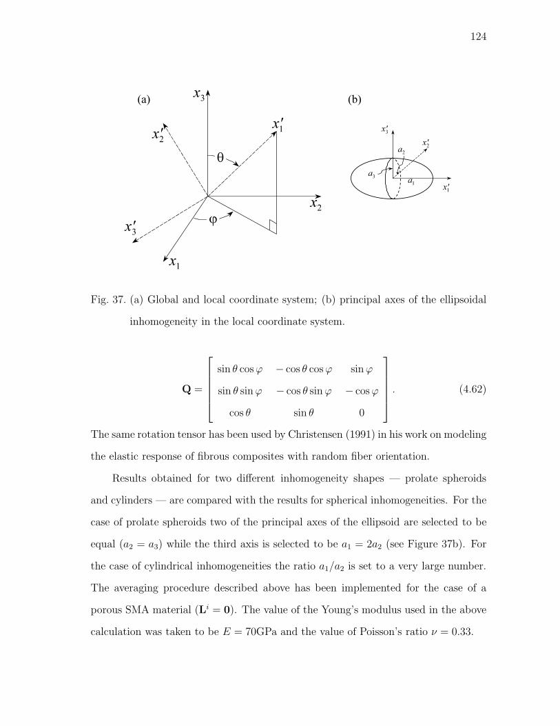
124

�

�

x1

x2

x3

�x1

�x2

�x3

�x1

�x2

�x3

a1

a3

a2

(a) (b)

Fig. 37. (a) Global and local coordinate system; (b) principal axes of the ellipsoidal

inhomogeneity in the local coordinate system.

Q =

sin θ cosϕ − cos θ cosϕ sinϕ

sin θ sinϕ − cos θ sinϕ − cosϕ

cos θ sin θ 0

. (4.62)

The same rotation tensor has been used by Christensen (1991) in his work on modeling

the elastic response of fibrous composites with random fiber orientation.

Results obtained for two different inhomogeneity shapes — prolate spheroids

and cylinders — are compared with the results for spherical inhomogeneities. For the

case of prolate spheroids two of the principal axes of the ellipsoid are selected to be

equal (a2 = a3) while the third axis is selected to be a1 = 2a2 (see Figure 37b). For

the case of cylindrical inhomogeneities the ratio a1/a2 is set to a very large number.

The averaging procedure described above has been implemented for the case of a

porous SMA material (Li = 0). The value of the Young’s modulus used in the above

calculation was taken to be E = 70GPa and the value of Poisson’s ratio ν = 0.33.

125

Young's Modulus

0.00

0.20

0.40

0.60

0.80

1.00

0 0.2 0.4 0.6 0.8 1

Pore volume fraction

No

rm

alize

d m

od

ulu

s

Spheres

Prolate Spheroids

Cylinders

Fig. 38. Normalized effective elastic Young’s modulus for porous SMA.

The averaging procedure results in isotropic effective material properties due to

the randomness of the orientation of the inhomogeneities. Results for the effective

Young’s modulus and effective bulk modulus are presented here. The values of these

material parameters are normalized by the corresponding matrix properties. The

values of the normalized effective Young’s modulus for different pore volume fractions

are plotted in Figure 38 and the normalized effective bulk modulus is plotted in

Figure 39. It is observed from these figures that there is a very slight difference

between the results for different pore shapes and there is a very good agreement,

especially between the results for the case of spherical pores and prolate spheroids.

A different approach for obtaining the effective properties of a composite with

random orientation of fibers has been presented by Christensen (1991). In his work

the averaging over all the possible fiber orientations is performed after obtaining the

effective properties of the composite with single fiber orientation. Using the present

notation, Christensen’s approach would be equivalent to calculating the effective stiff-

126

Bulk Modulus

0.00

0.20

0.40

0.60

0.80

1.00

0 0.2 0.4 0.6 0.8 1


No

rm

alize

d m

od

ulu

s

Spheres

Prolate Spheroids

Cylinders

Fig. 39. Normalized effective elastic bulk modulus for porous SMA.

ness as

L = Lm + (Li − Lm)

{{A[cmI + ciA

]−1}}

. (4.63)

The effective elastic stiffness calculated using equation (4.63) is also isotropic. How-

ever, it is noted that this method does not take into account the interactions among

inhomogeneities with different orientations. To compare the differences between the

two approaches the Young’s modulus of elasticity is calculated using equation (4.63)

and equation (4.60) for the case of random distribution of prolate spheroids and the

results are plotted in Figure 40. The same set of parameters as in Figures 38 and 39

is used. It can be seen from Figure 40 that for the current choice of parameters the

results of both methods are very close. This may be a reason why one would choose

to use equation (4.63), which is somewhat simpler, since it requires only one averag-

ing. However, equation (4.60) does not carry a significant additional computational

overhead and accounts for the interactions among inhomogeneities with different ori-

entations.

127

Young's Modulus

0.00

0.20

0.40

0.60

0.80

1.00

0 0.2 0.4 0.6 0.8 1


No

rmali

ze

d m

od

ulu

s

Present approach

Christensen (1991)

Fig. 40. Normalized effective Young’s modulus calculated using the present approach

[equation (4.60)] compared with the Young’s modulus calculated using the

approach by Christensen (1991) [equation (4.63)].

The results presented here are normalized and, therefore, are valid for all possible

values of the matrix stiffness. Thus, it is expected that the same result will hold if one

uses the tangent stiffness of the phases to obtain the effective properties of a porous

SMA undergoing a phase transformation.

Therefore, based on the above discussion, a spherical pore shape will be used to

represent the porosity in an SMA with a random distribution of pores. This shape

gives adequate representation of porosity and at the same time its use will greatly

reduce computational costs. Thus, a spherical pore shape will be used in all further

numerical calculations in this work.

4.2.2. Transformation Response

The determination of the transformation response of porous SMAs involves the so-

lution of equations (4.51) and (4.55) to obtain the values of the macroscopic stress

128

Σ and inelastic strain Ein for a given history of the overall strain E. To achieve

this, the tangent stiffness of the SMA matrix needs to be evaluated at every strain

increment. Due to the non-linearity of the problem, a numerical algorithm is utilized

in this work. A two-level numerical implementation is necessary: on the macroscopic

level the non-linearity is associated with the dependence of the strain concentration

factor Ai (and, therefore, Am) on the value of tangent stiffness of the SMA matrix;3

on the microscopic level the non-linearity is due to the non-linear constitutive SMA

model. The numerical implementation is described in detail in Chapter V.

To demonstrate the capabilities of the model numerical calculations for porous

SMA undergoing phase transformation have been performed. As a starting point

first the response during stable transformation cycle is modeled. To accomplish this

task, the material parameters for the SMA matrix are selected to correspond to NiTi

characterized in the work of Bo et al. (1999). These material parameters are presented

in Table I. Note that these parameters are for stable transformation cycle.

As a representative example numerical evaluations for the isothermal pseudoe-

lastic response of porous NiTi SMA were performed. The temperature was set to be

343 K. The numerical calculations were performed for an SMA prismatic bar under

uniaxial loading (see Figure 41). The numerical results were produced using a mesh

of two 3-D eight node solid elements, while identical results were obtained for a mesh

of eight 3-D elements, since both stress and strain are uniform. The axial effective

stress-strain response of the bar for various levels of porosity cp = 1− cm is shown in

Figure 42.

The results of Figure 42 indicate that the response of the material during trans-

3The Eshelby tensor SE entering the expression for the strain concentration factorAi is evaluated numerically, since in the case of general loading the tangent stiffnessof the SMA matrix is anisotropic. The method used for the evaluation of the Eshelbytensor is the one presented by Lagoudas et al. (1991).

129

�

Fig. 41. Schematic of the boundary-value problem for uniaxial loading of a prismatic

porous SMA bar.

formation strongly deviates from linearity which indicates that the tangent stiffness

tensor T continuously changes. This effect is caused by the change in the tangent

stiffness of the SMA matrix Tm. Since the Eshelby tensor used to evaluate the in-

stantaneous matrix strain concentration factor Am is calculated using the tangent

stiffness of the matrix, it is expected that the instantaneous strain concentration fac-

tor will vary significantly during the transformation. Thus it should be updated at

each loading increment.

Next the solution of equation (4.55), shown below for convenience is investigated.

Ein = (I− (Ael,m)−1Am) : E + (Ael,m)−1 : 〈ε∗m〉m − M : Σ︸︷︷︸︸︷︷︸︸︷︷︸term 1 term 2 term 3

(4.64)

It can be seen from equation (4.64) that there are three terms contributing to

the macroscopic inelastic strain. The first term is due to the difference between the

elastic and instantaneous strain concentration factors. In the case that Ael,m and

Am are the same this term will vanish. The second term represents the effect of the

130

0.00 0.02 0.04 0.06 0.08 0.10

Overall strain

0.00

100.00

200.00

300.00

400.00

500.00

600.00O

vera

ll s

tress

, M

PA


cp = 0.0 (Dense SMA)

cp = 0.1

cp = 0.2

cp = 0.3

cp = 0.4

cp = 0.5

Fig. 42. Effective stress-strain response of a porous NiTi SMA bar.

inelastic strain rate 〈ε∗m〉m in the matrix, which has three contributions, one from

the transformation strain, the second from the plastic strain and the third from the

stiffness change in the matrix [see equation (4.3)]. Note that the inelastic strain rate

is multiplied by the inverse of the elastic strain concentration factor (Ael,m)−1. The

third term is due to the change in the effective elastic compliance during the phase

transformation. Its physical meaning could be explained using the same arguments

made for the local stiffness change (see discussion in Section 4.1.1, Figure 35).

The contribution of each of the three terms to the macroscopic inelastic strain

Ein is examined for three different cases. The calculations for all of the three cases

are performed on a uniaxial SMA bar with 50% porosity for the loading path shown

in Figure 43. The difference between the three test cases is in the properties of the

SMA matrix.

131

Loading

Parameter

Ov

era

ll s

tress

0 0.5 1

max

�

Fig. 43. Loading history for uniaxial porous SMA bar.

In the first case it is assumed that the SMA matrix undergoes phase transforma-

tion and no plastic strains are accumulated. This case describes the situation where

the SMA matrix undergoes a stable transformation cycle. Therefore, the overall in-

elastic strain Ein becomes simply the overall transformation strain Et. The material

properties for this test case are the same used to obtain the results shown in Figure 42

and are summarized in Table I. The temperature for this case was set to be 343 K.

The normal components in the direction of the loading for each of the three terms

contributing to the effective transformation strain are plotted in Figure 44. It can be

seen that the contribution of the second term due to the local transformation strain is

dominant for the current choice of the material parameters. The contribution of the

first term is negative and lowers the value of the effective macroscopic transformation

strain. It can thus be seen from the figure that the effect of the difference between

the elastic and instantaneous strain concentration factors is not negligible. The third

term, which reflects the effect of the effective elastic compliance change has the small-

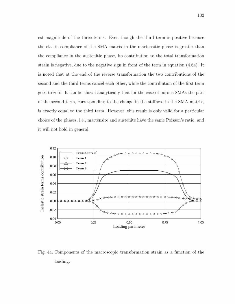
132

est magnitude of the three terms. Even though the third term is positive because

the elastic compliance of the SMA matrix in the martensitic phase is greater than

the compliance in the austenitic phase, its contribution to the total transformation

strain is negative, due to the negative sign in front of the term in equation (4.64). It

is noted that at the end of the reverse transformation the two contributions of the

second and the third terms cancel each other, while the contribution of the first term

goes to zero. It can be shown analytically that for the case of porous SMAs the part

of the second term, corresponding to the change in the stiffness in the SMA matrix,

is exactly equal to the third term. However, this result is only valid for a particular

choice of the phases, i.e., martensite and austenite have the same Poisson’s ratio, and

it will not hold in general.

0.00 0.25 0.50 0.75 1.00

Loading parameter

-0.04

-0.02

0.00

0.02

0.04

0.06

0.08

0.10

0.12

Inela

sti

c s

train

term

s c

ontr

ibu

tion

Transf. Strain

Term 1

Term 2

Term 3

Fig. 44. Components of the macroscopic transformation strain as a function of the

loading.

133

In the second test case it is assumed that the elastic properties of the martensite

and the austenite are the same, i.e., MM = MA. Then, the rate of inelastic strain in

the SMA matrix 〈ε∗m〉m becomes simply the rate of the transformation strain 〈εt,m〉min the second term, and the third term vanishes. To illustrate this special case, the

results of numerical calculations are show in Figure 45 for the same porous SMA

uniaxial bar with porosity of 50% as in the previous case. The material parameters

for this case are the ones shown in Table III for NiTi SMA tested by Strnadel et al.

(1995b). The temperature of the test was set to be 300 K. The values after the

stabilization of the transformation cycle (final values) of the material parameters are

used. The resulting normal strain components are shown in Figure 45. The same

general trend as in the previous case is observed (see Figure 44). However, in this

case the third term in equation (4.64) is zero.

The third test case is an extension of the second case and considers the situation

where both transformation and plastic strain are present. Thus, the inelastic strain

rate term in the SMA matrix contains both the rate of transformation strain and the

rate of plastic strain. To perform the numerical calculations for this test case the

same material properties as in the previous case are used (see Table III). However,

to be able to model the development of plastic strains both the initial and final sets

of parameters are used. Numerical simulations of one full transformation cycle are

performed at a temperature of 300 K.

The results showing the contribution of the different term on the overall inelastic

strain Ein are shown in Figure 46. Two effects manifesting the influence of the plastic

strain on the development of the overall inelastic strain are observed. First, since the

rate of the plastic strain in the matrix εp,m enters the second term in equation (4.64)

it is seen that its contribution at the end of the loading-unloading cycle does not

vanish. The second effect is due to the different tangent stiffness during loading and

134

0.00 0.25 0.50 0.75 1.00

Loading parameter

-0.02

0.00

0.02

0.04

0.06

Inela

sti

c s

train

term

s c

on

trib

uti

on

Transf. Strain

Term 1

Term 2

Term 3

Fig. 45. Components of the macroscopic transformation strain for the case of equal

stiffness of the austenite and martensite.

unloading. The difference in the tangent stiffness is caused by the development of

the plastic strain and it results in different evaluations of the instantaneous matrix

strain concentration factor Am during loading and unloading. Therefore, it is seen

that the total contribution of the first term [cf. equation (4.64)] at the end of the

transformation cycle does not vanish. These two effects result in the development

of non-zero total inelastic strain Ein at the end of the loading-unloading cycle. To

better illustrate the situation, the stress-strain curve for this test case is shown in

Figure 47. The residual macroscopic strain at the end of the cycle (at zero applied

stress) seen in the figure is caused by the two effects discussed here.

135

0.00 0.25 0.50 0.75 1.00

Loading parameter

-0.02

0.00

0.02

0.04

0.06

Inela

sti

c s

train

term

s c

ontr

ibuti

on

Inelastic Strain

Term 1

Term 2

Term 3

Fig. 46. Components of the macroscopic inelastic strain as a function of the loading

(both plastic and transformation strains are present).

136

0.00 0.01 0.02 0.03 0.04 0.05 0.06 0.07

Overall strain

0.00

50.00

100.00

150.00

200.00

250.00

300.00

Overa

ll s

tress

, M

PA

Fig. 47. Effective stress-strain response of a porous NiTi SMA bar (both plastic and

transformation strains are present).

137

CHAPTER V

NUMERICAL IMPLEMENTATION OF THE MODEL FOR POROUS SMAS

AND COMPARISON WITH EXPERIMENTAL RESULTS

In this chapter the micromechanical model presented in Chapter IV will be numeri-

cally implemented and used to simulate the experimental results for mechanical load-

ing of porous NiTi. First the material parameters of the porous NiTi will be estimated.

As a next step the test results will be simulated using the model. Finally different

loading cases will be performed to test the capabilities of the model.

5.1. Numerical Implementation of the Micromechanical Model for Porous SMAs

This section addresses the implementation of the micromechanical model for porous

SMAs. This implementation utilizes the earlier established procedure for numeri-

cal integration of the constitutive equations for the fully dense SMA, presented in

Chapter III. The implementation presented here is valid for a displacement-based

formulation (e.g., a finite element formulation) where the history of the overall strain

E(t) is given. Note that an additional non-linearity is introduced due to the depen-

dance of the strain concentration factors on the current tangent stiffness in the SMA

matrix. This additional difficulty is resolved by employing a direct iteration (Picard

iteration) method, as described in a sequel.

The numerical implementation involves the following iterative procedure: first,

the elastic stiffness of the SMA matrix is used to calculate the Eshelby tensor and

the strain concentration factor Am; once the current value of the strain concentration

factor Am is known, it is used to obtain the strain increment in the SMA matrix

∆εm from the given increment of the overall strain ∆E; if the phase transformation

condition in the matrix is satisfied, then the return mapping algorithm presented in

138

Section 3.1 is then used to update the values of the stress, transformation strain,

plastic strain, martensitic volume fraction and tangent stiffness in the matrix; finally,

a new value of the strain concentration factor is obtained using these updated results.

The direct iteration procedure terminates after the difference between two suc-

cessive values of the strain concentration factor is less than a given tolerance. At

this point the obtained final values of the stress, transformation strain, plastic strain,

martensitic volume fraction and the strain concentration factor are used to obtain

the effective tangent stiffness and the increment of the effective inelastic strain using

equations (4.51) and (4.55). The steps of the iterative procedure are summarized in

Table IV.

Table IV. Implementation of the incremental micromechanical averaging method for

porous SMAs.

1. Set k = 0, Tm(0) = Lm.

2. Calculate Eshelby tensor SE(k) using Tm(k), calculate average instantaneous

strain concentration factor Am(k):

Am(k) =1

cm

(I − (1 − cm)

[I + cmSE(k)

]−1)

3. Calculate the increment of strain in the matrix ∆εm(k):

∆εm(k) = Am(k) : ∆E

4. The return mapping algorithm for dense SMAs (Table II) is called with

∆εm(k) as its input. The output of the algorithm are the updated value

of the stress in the matrix σm(k+1), martensitic volume fraction ξ(k+1),

transformation and plastic strain εtm(k+1), εpm(k+1) and the tangent stiffness

tensor of the SMA matrix Tm(k+1).

139

Table IV. Continued.

5. Calculate Eshelby tensor SE(k+1) using Tm(k+1), calculate average

instantaneous strain concentration factor Am(k+1).

6. If∣∣Am(k+1) − Am(k)

∣∣ > TOL2 then

set k = k + 1;

go to 3.

7. Calculate the overall tangent stiffness tensor T and the increment of the

inelastic strain ∆Ein:

T = cmTmAm

∆Ein = (I − (Ael,m)−1Am) : ∆E + (Ael,m)−1 : 〈∆ε∗m〉m − ∆M : Σ

Note that in the implementation of the micromechanical averaging method the

strain in the SMA matrix becomes another internal state variable. It must be updated

and stored at each load increment. The number of Picard iterations depends on the

value of tolerance TOL2 and on the number of the load increments. For tolerance

TOL2 = 1.0 × 10−9 and 100 load increments 5–8 iterations are performed before a

convergence is achieved.

5.2. Uniaxial Porous NiTi Bars under Compression

Porous NiTi specimens were fabricated from elemental Ni and Ti powders using HIP-

ping techniques in the Active Materials Laboratory at Texas A&M University (Vandy-

griff et al., 2000). Using two slightly different processing cycles two different porous

NiTi alloys were produced. The first alloy was fabricated at a temperature of ≈ 940�C

and is characterized by its small pore size (on the order of 25 µm). The fabrication

temperature for the second alloy was ≈ 1000�C and the sizes of its pores are sig-

140

nificantly larger (pores as large as 1 mm are observed). A detailed analysis of the

composition of the two alloys was performed by Lagoudas and Vandygriff (2002) using

Energy-Dispersive X-ray Spectrometry (EDS) and further using Wave-Dispersive X-

ray Spectrometry (WDS). The analysis has revealed evidence of multiple intermetallic

phases present in both large and small pore alloys. The greater part of the mate-

rial for large pore alloys was identified as equiatomic NiTi. However, the material

contains numerous needle-like structures having a width of approximately one-half

micron. These needle-like structures were too small to be analyzed without interfer-

ence from the surrounding medium. By analyzing some of the larger intersections of

needle-like phases however, it is presumed by a slight increase in the percentage of

Ni that the needle phases are Ni rich phases. For the small pore alloy five different

phases, i.e., NiTi, Ni2Ti, NiTi3 and elemental Ni and Ti were identified. The appar-

ent reason for the presence of relatively large intermetallic phase regions in the small

pore alloy is the lower fabrication temperature, which leads to incomplete diffusion

of the elemental powders.

The porosity of the specimens was measured by taking micrographs and esti-

mating the ratio of the area occupied by the pores to the total area at different

cross-sections. The estimate of the porosity was also verified by comparing the den-

sity of the porous NiTi material with the theoretical density of fully dense NiTi. The

porosity of the small pore alloy is estimated to be equal to 50% while the porosity

of the large pore alloy is equal to 42%. Micrographs of typical specimens for both

small and large pore alloys are shown in Figures 48 and 49. The dark areas on the

micrographs, shown in Figures 48 and 49 represent the pores, while the lighter areas

are occupied by NiTi.

The porous NiTi specimens were further analyzed using differential calorimetry

techniques. The DSC test curves for both small and large pore alloys are shown

141

50 �m

Fig. 48. Microphotograph of a small pore porous NiTi specimen.

in Figures 50 and 51, respectively. The upper curves seen in Figures 50 and 51

represent the normalized heat flow into the specimen during heating and the lower

curves represent the heat flow out of the specimen upon cooling. The tests indicate

solid-solid phase transformation at approximately 44�C and 42�C for the small and

large pore alloys during heating (martensite-to-austenite) and −12�C and 20�C during

cooling (austenite-to-martensite) for the small and large pore specimens, respectively.

Therefore, depending on whether the specimen was previously heated or cooled, either

martensite or austenite crystalline structure can be present at room temperature

(22�C). The cooling curves for both alloys show evidence of a dual peak that is

indicative of an R-phase.

The fabricated porous NiTi specimens have a cylindrical shape with a nominal

diameter of 13 mm and a length of 35 mm. The specimens were mechanically tested

under compressive load. Load from a hydraulic MTS load frame was applied through

two compression plates. An extensometer was used to take the strain measurements

during testing. The specimens were tested using a cyclic loading-unloading pattern

142

1 mm

Fig. 49. Microphotograph of a large pore porous NiTi specimen.

by loading quasi-statically up to a stress and strain level and then unloading to

zero stress. For each subsequent cycle, the stress and/or strain were increased with

respect to the previous level. The resulting stress-strain response for a typical small

pore specimen, tested at a temperature of 60�C is shown in Figure 52 and shows

evidence of pseudoelastic behavior upon unloading. However, full strain recovery is

not observed, which is due to plastic strain development in the SMA matrix. The

typical stress-strain response for a large pore specimen also tested at 60�C is shown

in Figure 53. The results for the second specimen are qualitatively similar to the

result for the small pore specimen. However, certain distinctions are observed from

Figures 52 and 53. The initial tangent stiffness of the austenite and martensite are

different in the two specimens. The approximate stiffness of the austenite phase in

the large pore specimen is approximately 15 GPa, about twice that of the small pore

austenite phase stiffness of 7 GPa. This difference in the stiffness may be partially due

to incomplete diffusion of the powders in the small pore specimen and the resulting

partial adherence of the powder particles. The difference in the pore volume fraction

143

Fig. 50. DSC results for small pore porous NiTi alloy.

of the two types of specimens also contributes to the difference in the stiffness. Thus,

while the maximum reached strain level for the two specimens is similar, the stress

levels differ significantly.

When a large pore specimen is loaded to strain levels beyond 5% it starts to

fail by forming microcracks, which was evident by the cracking and popping noises

during loading. This failure is identified on the stress-strain curve by the decrease of

the stress as the strain is increased (Figure 53). On the other hand the small pore

specimens failed catastrophically, forming large cracks that propagated throughout

the entire specimen, causing the specimen to break into multiple fragments.

5.2.1. Estimation of the Material Properties for Porous NiTi

Using the experimental data presented in Figures 50–53 the material parameters for

both types of porous NiTi alloy are estimated in this section. First, the estimation of

the parameters for the small pore NiTi alloy is presented. The procedure presented

here is outlined in Section 2.7. Care must be exercised when taking into account the

144

Fig. 51. DSC results for large pore porous NiTi alloy.

porosity. The values of the stress appearing during the estimation of the parameters

in Section 2.7 must be calculated for the SMA matrix. Therefore, to connect the stress

in the matrix with the applied stress, the Mori–Tanaka method is used. Only one

set of material parameters is obtained, since the experimental data is not sufficient

to obtain complete two sets (initial and final, see Sections 2.5, 2.7).

First the material parameters for a transformation cycle without plastic strains

are estimated. To accomplish this, the residual plastic strain after each increment

is subtracted from the total strain. Thus, only the elastic/phase transformation

response is obtained (see Figure 54). The material parameters are estimated for

a transformation loop which is the envelope of the experimental results shown in

Figure 54.

To proceed with the estimation of the material properties, it is assumed that the

SMA matrix is isotropic with Poisson’s ratio νA = νM = 0.33. Next, the Young’s

elastic moduli of austenite and martensite are evaluated by solving the inverse Mori–

Tanaka problem for the porous material and using the experimental data. The value

145

0.000 0.005 0.010 0.015 0.020 0.025 0.030 0.035 0.040 0.045

Macroscopic Strain

0.0

20.0

40.0

60.0

80.0

100.0

120.0M

acro

scopic

Str

ess

, M

Pa

Fig. 52. Stress-strain response of small pore porous NiTi alloy tested at 60�C.

of the effective Young’s modulus of the porous austenite is measured using the slope

at the beginning of the loading (see Figure 54) and the corresponding value of the

Young’s modulus for the austenitic matrix is evaluated from the inverse Mori–Tanaka

method to be EA = 19.7 GPa. Similarly, the value of the effective Young’s modulus of

the porous martensite is obtained using the unloading slope of the last loading cycle

(see Figure 54), which results in EM = 19.0GPa. The values of the thermal expansion

coefficient for martensite and austenite are taken from the work of Lagoudas and Bo

(1999) and are equal to αA = 11.0×10−6 K−1 and αM = 6.0×10−6 K−1. Similarly, the

values of the specific heat constants cA and cM are obtained from the literature (Bo

146

0.00 0.01 0.02 0.03 0.04 0.05 0.06

Macroscopic Strain

0.0

50.0

100.0

150.0

200.0

250.0M

acro

scopic

Str

ess

, M

Pa

Fig. 53. Stress-strain response of large pore porous NiTi alloy tested at 60�C.

and Lagoudas, 1999a). Since the loading cases considered in this work are isothermal,

the last four constants will not have any effect on the numerical results, but they are

still necessary for successful runs of the numerical code.

The martensitic start temperature M0s is determined from the calorimetric test

data, shown in Figure 50. As explained earlier, the cooling curve in Figure 50 shows

evidence of a dual peak that is indicative of an R-phase. The second peak was used

to obtain the value of the martensitic start temperatures M0s = 269.5 K.

The experimental stress-strain curves shown in Figure 52 differ from the stress-

strain response expected for NiTi. Namely, it is expected that after initial hardening

147

0.000 0.005 0.010 0.015 0.020 0.025 0.030 0.035

Macroscopic Strain

0.0

20.0

40.0

60.0

80.0

100.0

120.0

Macro

scopic

Str

ess

, M

Pa

Fig. 54. Elastic/phase transformation stress-strain response of small pore porous NiTi

alloy.

the pseudoelastic stress-strain curve reaches a plateau with subsequent hardening af-

ter the phase transformation is complete. However, the results shown in Figure 52

reach a plateau without exhibiting the second hardening. In addition, the value of the

recovered transformation strain is smaller than expected for a NiTi alloy. Therefore,

these results suggest that the material does not undergo full austenite-to-martensite

phase transformation. Thus, the value of the maximum transformation strain can-

not be accurately obtained using the available experimental data. To overcome this

148

difficulty a value of the maximum transformation strain H = 3% which is typical

for NiTi has been used in this work. Then, it follows that the maximum value of

the martensitic volume fraction ξ reached during the stress loading is approximately

equal to 0.5. The value of the material parameter ρ∆s0 is estimated to be equal to

−0.03 MJ/(m3K) where equation (2.76) has been utilized by calculating the value of

the stress in the matrix using the Mori–Tanaka method. The value of the material

parameter Y is estimated to be equal to Y = 1.3 MJ/m3.

There is no available data on the dependance of the current maximum trans-

formation strain Hcur on the value of the applied stress for this alloy. Therefore, to

evaluate the drag stress parameters the data for a dense NiTi alloy shown in Figure 14

is used with an appropriate scaling such that the maximum transformation strain for

high values of stress is equal to the maximum transformation strain H = 0.03. The

back stress parameters Dd1, D

d2 and m1 are evaluated by curve-fitting of the transfor-

mation stress-strain curve during forward transformation. The parameter governing

the curvature of the minor transformation loops is estimated to be γ = 4.0. The

comparison of the model simulations for one loop using the estimated parameters

with the experimental stress-strain data is shown in Figure 55. It can be seen that

the simulation results closely match the experimental curve.

Once the parameters for a single transformation cycle are determined, the only

unknowns are the parameters connected with the development of the plastic strains.

To obtain the values of the parameters Cp1 and Cp

2 one must have data on the evolution

of plastic strain with the number of cycles. Since the loading cycles performed during

the experiments are not complete, to establish the values of the parameters, a slightly

different procedure than the one described in Section 2.7 is used. First the model is

used to establish the values of the internal parameter ζd at the end of each loading

cycle. Next, the value of the plastic strain at the end of each loading cycle is found

149

0.000 0.005 0.010 0.015 0.020 0.025 0.030 0.035

Macroscopic Strain

0.0

20.0

40.0

60.0

80.0

100.0

120.0

Macro

scopic

Str

ess

, M

Pa

Experiment

Model

Fig. 55. Comparison of the experimental elastic/phase transformation stress-strain

response of small pore porous NiTi alloy with the model simulations.

from the experimental results. Thus, the relationship between the plastic strain and

the accumulated detwinned martensitic volume fraction is found. Using this data

and equation (2.81) the values of the parameters Cp1 and Cp

2 are estimated. Note that

the procedure presented in Section 2.7 can still be utilized if complete transformation

cycles were performed. The complete set of material parameters for the small pore

NiTi alloy is summarized in Table V.

The material parameters for the large pore porous NiTi alloys are estimated

150

Table V. Material parameters for small pore porous NiTi SMA.

Physical constants

EA = 19.7 GPa αA = 11.0 × 10−6 K−1

EM = 19.0 GPa αM = 6.6 × 10−6 K−1

ρcA = 2.12 MJ/(m3K) ν = 0.33

ρcM = 2.12 MJ/(m3K)


M0s = 269.5 K ρ∆s0 = −0.03 MJ/(m3K)

H = 0.03 Y = 1.3 MJ/m3

Db1 = 7.83 × 103 MPa Dd

1 = 2.0 MPa

Db2 = −1.18 × 106 MPa Dd

2 = −2.5 MPa

Db3 = 1.01 × 108 MPa m1 = 3.5

Db4 = −4.19 × 109 MPa

Db5 = 6.61 × 1010 MPa


γ = 4.0

Parameters characterizing the accumulation of plastic strain

Cp1 = 6.0 × 10−3

Cp2 = 1.66

151

following the same procedure and using the data shown in Figures 51 and 53. Only

the data before the occurring of the microcracking is used to estimate the material

parameters. They are summarized in Table VI.

It is noted that the obtained material parameters for both small and large pore

porous NiTi are different from the ones used earlier in Chapter II. This difference

can be explained by the different processing parameters of the material. The material

parameters in Chapter II are obtained for NiTi wires, which have a substantial amount

of cold work, as well as different heat treatments from the porous SMA material, which

has not been cold worked.

5.2.2. Comparison of the Experimental Results with Model Simulation

A finite element model reflecting the geometry of a typical specimen (diameter of

13 mm and length of 35 mm) is constructed. The domain is discretized using eight-

node quadratic axisymmetric elements. In order to allow for both compression and

combined compression-torsion loading, results of which are presented in a sequel,

elements with a twist degree of freedom were used. Since the axial stress does not

vary for both loading cases, only one layer of elements in the axial direction is used.

The length of the elements in the axial direction is chosen to be 1.75 mm. To capture

the stress variation in the radial direction, 5 elements are used. The finite element

mesh and the loading history are shown in Figure 56.

The comparison of the compressive stress-strain response for the small pore NiTi

alloy simulated by the model with the experimental data is shown in Figure 57.

The material properties presented in Table V have been used during the numerical

calculations. Overall, very good agreement between the results is obtained. Several

observations are made from Figure 57. First, the effective Young’s moduli for both

austenite and martensite are correctly reproduced by the model, since their values

152

Table VI. Material parameters for large pore porous NiTi SMA.

Physical constants

EA = 42.0 GPa αA = 11.0 × 10−6 K−1

EM = 32.0 GPa αM = 6.6 × 10−6 K−1

ρcA = 2.12 MJ/(m3K) ν = 0.33

ρcM = 2.12 MJ/(m3K)


M0s = 293.0 K ρ∆s0 = −0.05 MJ/(m3K)

H = 0.03 Y = 3.0 MJ/m3

Db1 = 7.83 × 103 MPa Dd

1 = 12.0 MPa

Db2 = −1.18 × 106 MPa Dd

2 = 1.0 MPa

Db3 = 1.01 × 108 MPa m1 = 3.5

Db4 = −4.19 × 109 MPa

Db5 = 6.61 × 1010 MPa


γ = 1.0

Parameters characterizing the accumulation of plastic strain

Cp1 = 1.99 × 10−2

Cp2 = 1.51

153

35 mm

13 mm

(a)

0z

u u�

� �

0r

u �

Applied compression

(c)

axis of

symmetry

z

r

Loading

Parameter

zu�

1.0

max

zu

0.5

(b)

Fig. 56. Compressive loading of a porous NiTi SMA bar: (a) geometry; (b) loading

history; (c) boundary conditions.

have been used for the model calibration. The slope of the stress-strain curve during

the transformation is in good agreement with the experimental data. The behavior

of the material during minor loops is also correctly reproduced.

Next, the comparison of the plastic strain predicted by the model with the plastic

strain developed during the testing of the material is presented. As explained earlier,

the evolution of plastic strain in the direction of the loading Ep is presented as a func-

tion of the accumulated detwinned martensitic volume fraction ζd. The comparison

of the model simulation with the experimental data is shown in Figure 58. It can be

seen that the model simulation closely follows the experimental results.

Similar results have been calculated for the large pore porous NiTi alloy using the

material parameter shown in Table VI. The comparison of the numerical results with

the experimental stress-strain data is shown in Figure 59. It can be seen that despite

some discrepancies, the results of the numerical simulations are in good agreement

with the experimental data. The plot of the plastic strain versus the accumulated

detwinned martensitic volume fraction is shown in Figure 60.

154

0.000 0.005 0.010 0.015 0.020 0.025 0.030 0.035 0.040 0.045

Macroscopic Strain

0.0

20.0

40.0

60.0

80.0

100.0

120.0

Macro

scopic

Str

ess

, M

Pa

Experiment

Model

Fig. 57. Stress-strain response of a small pore porous NiTi SMA bar — comparison

between the experimental results and the model simulation.

One reason for the observed discrepancies may be due to the development of

microcracks in the specimen during testing. As mentioned earlier, the large pore

NiTi alloy under compressive testing started failing by developing microcracks. Even

though attempts were made to eliminate the effect of the microcracking by considering

only the results before it occurred some failure may have occurred earlier. The stress-

strain response during the last three loading cycles is shown in Figure 61. It can be

seen that starting with the 7th loading cycle the results of the model substantially

deviate from the experimental results. It is evident from the change in the slope of the

experimental stress-strain curve that there are some changes in the properties of the

alloy. A micrograph of the large pore specimen after testing is shown in Figure 62. The

155

0.0 1.0 2.0 3.0 4.0

�d

0.0

0.0

0.0

0.0

0.0

0.0

E p

Model

Experiment

Fig. 58. Plastic strain Ep versus accumulated detwinned martensitic volume fraction

ζd for the small pore porous NiTi.

figure shows that microcracks propagate through the pore walls. Thus, the change in

the stiffness of the specimen after the loading can be attributed to the development

of these microcracks.

One can attempt to improve the model simulations by eliminating the last two

loading cycles and modifying the plastic strain evolution constants Cp1 and Cp

2 such

that a better simulation of the plastic strain is obtained. Thus, if the new values

for the constants are selected to be Cp1 = 0.052 and Cp

2 = 0.25 the resulting plastic

strain evolution as predicted by the model is shown in Figure 63. The corresponding

stress-strain response is shown in Figure 64. It can be seen from these figures that

the results of the model simulations are in good agreement with the experimental

observations.

156

0.000 0.005 0.010 0.015 0.020 0.025 0.030 0.035 0.040 0.045 0.050 0.055

Macroscopic Strain

0.0

25.0

50.0

75.0

100.0

125.0

150.0

175.0

200.0

225.0

250.0

Macro

scopic

Str

ess

, M

Pa

Experiment

Model

Fig. 59. Stress-strain response of a large pore porous NiTi SMA bar — comparison

between the experimental results and the model simulation.

157

0.0 0.5 1.0 1.5 2.0 2.5

�d

0.000

0.005

0.010

0.015

0.020

0.025

E p

Experiment

Model


ζd for the large pore porous NiTi.

158

0.010 0.015 0.020 0.025 0.030 0.035 0.040 0.045 0.050 0.055

Macroscopic Strain

0.0

25.0

50.0

75.0

100.0

125.0

150.0

175.0

200.0

225.0

250.0

Macro

scopic

Str

ess

, M

Pa

Experiment

Model

6th loading cycle

7th loading cycle

8th loading cycle

Fig. 61. Stress-strain response of a large pore porous NiTi SMA bar — last three

loading cycles.

cracks

Fig. 62. Microcracking of the large pore porous NiTi SMA bar during mechanical

loading.

159

0.0 0.5 1.0 1.5

�d

0.000

0.004

0.008

0.012

0.016

E p

Experiment

Modified model


ζd for the large pore porous NiTi using the modified plastic strain evolution

constants.

160

0.000 0.005 0.010 0.015 0.020 0.025 0.030 0.035 0.040

Macroscopic Strain

0.0

25.0

50.0

75.0

100.0

125.0

150.0

175.0

200.0

225.0

Macro

scopic

Str

ess

, M

Pa

Experiment

Corrected model

Fig. 64. Stress-strain response of a large pore porous NiTi SMA bar using the modified

plastic strain evolution constants.

161

5.3. Porous NiTi Bars under Multiaxial Loading

The loading cases described above represent uniaxial loading of porous SMA bars.

However, most engineering applications require the capability to handle more complex

loading paths, involving multiaxial non-proportional loading. It is envisioned that the

capability to model such loading cases will become increasingly important as porous

SMAs are used in various new applications, such as vibration isolation of multiple

degrees of freedom and biomedical applications. In addition, the modeling of complex

loading paths will facilitate experimental work, which will provide results necessary

for the calibration of the model, which is three dimensional.

5.3.1. Compression-Torsion Loading of Porous SMA Bars

To test the capabilities of the model, the response of the small pore NiTi porous

SMA bar with 50% porosity, described in Section 5.2, is modeled under combined

compression-torsion loading. Different loading cases were tested: compression-torsion,

torsion-compression as well as simultaneous compression-torsion. The boundary con-

ditions and the loading histories for these cases are shown in Figure 65 while the

finite element mesh is the same as shown in Figure 56a. The maximum value of the

applied rotation (see Figure 65) was taken to be θmax = 0.02 rad (≈ 1.15�), which

corresponds to ≈ 11.4 rad/m (≈ 1.8 full revolutions per meter) rotation, while the

maximum value of the displacement in the axial direction during the second loading

step was taken to be umaxz = −0.125 mm, corresponding to macroscopic axial com-

pressive strain of Ezz = 0.071. Both compression and rotation boundary conditions

were applied on the top surface of the specimen, while the bottom surface was held

fixed in the z− and θ− directions. Traction-free boundary condition in the radial

direction was applied. The numerical simulations were performed at temperature of

162

60�C. The analyses were performed on a single processor Digitaltm Alpha 600AU

workstation. Forty eight loading increments were performed to complete both load-

ing and unloading steps and the CPU time required to perform the computations

varied between 32.0 sec for the case of combined loading to 48.7 sec for the case of

torsion-compression loading.

(a) (b)

Torsion-compression

Loading

Parameter

u�

zu

1max

zu

max

u�

Compression-torsion

Combined

0z

u u�

� �

0r

u �

Applied rotation

and compression

axis of

symmetry

z

r

0.5

Fig. 65. Schematic of the BVP for compression-torsion multiaxial loading of a porous

SMA bar: (a) boundary conditions; (b) loading histories.

The history of the stresses and the martensitic volume fraction for the three cases

are shown in Figure 66 for an element positioned at the outer surface of the bar. It

is seen that the results for the combined compression-torsion loading case resemble

superposition of the results under compression and torsion applied independently,

while for the case of compression-torsion the material fully transforms during the

compressive loading (depending on the value of the imposed axial strain) and the

response under torsion is elastic. Thus only the results for the torsion-compression

loading are presented in greater detail.

The contour plot of the martensitic volume fraction in the SMA matrix at the

163

0.00 0.25 0.50 0.75 1.00

Loading parameter

0.0

0.2

0.4

0.6

0.8

1.0

��

Compression-torsion

Combined loading

Torsion-compression

0.00 0.25 0.50 0.75 1.00

Loading parameter

-200

-150

-100

-50

0

Sh

ear

stre

ss �� z

��(M

Pa)

0.00 0.25 0.50 0.75 1.00

Loading parameter

-400

-300

-200

-100

0

Axia

l st

ress

�� z

z (

MP

a)

Fig. 66. History of the axial stress, shear stress and the martensitic volume fraction

during torsion-compression loading.

164

VALUE+0.00E-00

+5.06E-02

+1.02E-01

+1.54E-01

+2.06E-01

+2.58E-01

+3.10E-01

+3.61E-01

+4.13E-01

+4.65E-01

+5.17E-01

+5.69E-01

+6.21E-01

+6.72E-01

�

Axis of symmetry

Element used to plot stresses

Fig. 67. Contour plot of the martensitic volume fraction in the porous NiTi SMA bar

at the end of the torsional loading.

end of the torsional loading (the value of loading parameter equals to 0.5) for the

porous bar is shown in Figure 67. It is observed from the figure that the contours

corresponding to the same value of ξ are concentric circles. The maximum value of

the martensitic volume fraction is ξ = 0.67 at the external boundary of the bar, where

the shear stress is maximum, while its minimum value is ξ = 0.0 close to the center

of the bar.

Next, the history of the stresses and the martensitic volume fraction are shown

165

for an element positioned at the outer surface of the bar (the element is indicated

in Figure 67). For comparison purposes, the same loading case was tested on a fully

dense NiTi SMA bar with the same geometry and the same material properties. The

same finite element mesh of 100 quadratic axisymmetric elements as in the case of

compressive loading was used. The average values of the axial and shear stress and

the average value of the martensitic volume fraction versus the loading parameter

for both the porous and the fully dense SMA bar are plotted on Figure 68. It can

be seen from the results that initially the porous SMA material behaves elastically,

with the onset of the phase transformation near the value for the loading parameter

of about 0.15. The partial phase transformation continues to the end of the torsional

loading (the value of the loading parameter is 0.5). Next, with the application of

compressive loading, the phase transformation continues and it is fully completed

close to the value of the loading parameter of 0.85. Due to the phase transformation

during the compressive loading the shear stress Σzθ is partially relaxed, as indicated

in Figure 68. Upon further loading the material behaves elastically with the elastic

properties of martensite.

Similar trends are observed for the case of the dense SMA bar, but the stress

values are much higher than the ones in the case of the porous bar. The results

shown in Figure 68 are also compatible with the results for thin fully dense SMA

tubes presented in Chapter II.

166

Fully dense NiTi SMA

Porous NiTi SMA - 50% porosity

0.00 0.25 0.50 0.75 1.00

Loading parameter

-300

-250

-200

-150

-100

-50

0

Shear

stre

ss �� z

��(M

Pa)

0.00 0.25 0.50 0.75 1.00

Loading parameter

0.0

0.2

0.4

0.6

0.8

1.0

��

0.00 0.25 0.50 0.75 1.00

Loading parameter

-1000

-800

-600

-400

-200

0

Axia

l st

ress

�� z

z (

MP

a)

Fig. 68. History of the axial stress, shear stress and the martensitic volume fraction

during torsion-compression loading.

167

5.3.2. Three-Dimensional Effects during Compressive

Loading of Porous SMA Bars

As mentioned before, the tested porous SMA bars have nominal diameter of 13 mm

and length of 35 mm. Since the length/diameter ratio is not very large, the compres-

sive loading may result in three-dimensional stress state, due to the traction between

the specimen and the compressive plates. To examine the three-dimensional effects,

a boundary-value problem using the geometry of the whole bar and the appropriate

boundary conditions is analyzed. The computational domain is discretized using 100

axisymmetric quadratic elements, as shown in Figure 69.

0z r

u u u�

� � �

0r

u �

Applied compressionz

r

axis of

symmetry

0,r z

u u u const�

� � �

Fig. 69. Schematic of the BVP for compressive loading of a porous SMA bar with

constrained surfaces.

To account for the traction between the specimen and the compressive plates, the

168

top and bottom surfaces are constrained in the radial direction, as shown in Figure 69.

In addition, the top surface if constrained in the axial direction using a multi-point

constraint such that it remains planar. The compressive loading is applied on the

top surface. The applied force is selected to be the same as in the case of uniaxial

loading, presented in Section 5.2.1.

The material parameters for the small pore NiTi alloy are used (see Table V).

For simplicity, it is assumed that no plastic strains develop. The effective stress is

obtained by calculating the ratio of the applied force to the area of the bar and the

effective strain is calculated as the ratio of the displacement of the top surface to the

initial length of the bar. The effective stress-strain response of the porous SMA bar is

shown in Figure 70, where it is also compared with the uniaxial response, presented

in Section 5.2.1. It can be seen that the effective response of the bar, calculated by

taking into account the three-dimensional effects, deviates from the uniaxial response.

To further examine the three-dimensional effects, the von Mises effective stress

in the bar is analyzed. The contour plot of the von Mises stress at the end of the

loading is plotted in Figure 71. It can be seen, that near the top and bottom surfaces

the stress is very non-uniform, while it is uniform in the middle part of the bar. The

non-uniformity is due to the applied constraints on the surfaces. The constraint in the

radial direction results in compressive stresses being developed in the radial direction

as well as in stress concentrations near the outer surface of the bar. The compressive

stresses decrease the value of the von Mises effective stress near the center of the bar,

as seen in Figure 71. As a result of the decrease in the effective stress, the phase

transformation in these regions takes place slower than in the middle of the bar. This

effect can be observed by analyzing the contour plot of the martensitic volume fraction

in the porous SMA bar, shown in Figure 72. As seen from Figure 72, the values of the

martensitic volume fraction are significantly lower near the top and bottom surfaces

169

0.000 0.005 0.010 0.015 0.020 0.025 0.030 0.035

Macroscopic Strain

0.0

20.0

40.0

60.0

80.0

100.0

120.0

Macro

scopic

Str

ess

, M

Pa

Uniaxial

Three-dimensional

Fig. 70. Stress-strain response of a small pore porous NiTi SMA bar showing the

three-dimensional effect during compressive loading.

of the bar. The net effect of the lower value of the martensitic volume fraction in

these regions is the apparent stiffer effective response, as seen in Figure 70.

170

V. MISES VALUE

+4.89E+07

+5.67E+07

+6.45E+07

+7.23E+07

+8.01E+07

+8.79E+07

+9.57E+07

+1.04E+08

+1.11E+08

+1.19E+08

+1.27E+08

+1.35E+08

+1.43E+08

+1.50E+08

Axis of symmetry

Fig. 71. Contour plot of von Mises effective stress in the porous SMA bar at the end

of the compressive loading.

171

� VALUE

+2.65E-02

+7.19E-02

+1.17E-01

+1.63E-01

+2.08E-01

+2.54E-01

+2.99E-01

+3.44E-01

+3.90E-01

+4.35E-01

+4.81E-01

+5.26E-01

+5.71E-01

+6.17E-01

Axis of symmetry

Fig. 72. Contour plot of the martensitic volume fraction in the porous SMA bar at

the end of the compressive loading.

172

CHAPTER VI

CONCLUSIONS AND FUTURE WORK

6.1. Summary and Conclusions

The development of a macroscopic constitutive model for porous SMAs has been

presented in this work. The model is derived using micromechanical averaging tech-

niques. The porous SMA material is modeled as a two-phase composite with an

SMA matrix and a second phase which represents the pores. The behavior of the

dense SMA matrix is modeled using a rate-independent thermomechanical constitu-

tive model with internal variables. The evaluation of the material parameters for

the porous SMA material has been presented for two NiTi alloys fabricated from

elemental powder sintering. The major findings and contributions of this work are

summarized below.

In the first part of the current work the derivation of a three-dimensional ther-

momechanical constitutive model for fully dense SMAs has been presented. In the

current formulation of the model the following quantities are chosen as internal state

variables: martensitic volume fraction, transformation strain, plastic strain, back

stress and drag stress. The evolution equations for these parameters for the case of

a three-dimensional loading have been presented. It should be noted that the plastic

strain adopted in this work differs from the plastic strain in regular metal plasticity.

The plastic strain defined in this work is induced by the martensitic phase transfor-

mation at relatively low values of the applied stress. The evolution equations for the

plastic strain have been chosen to accurately represent the case of a material under-

going stress-induced martensitic phase transformation and differ from the ones given

by Bo and Lagoudas (1999a).

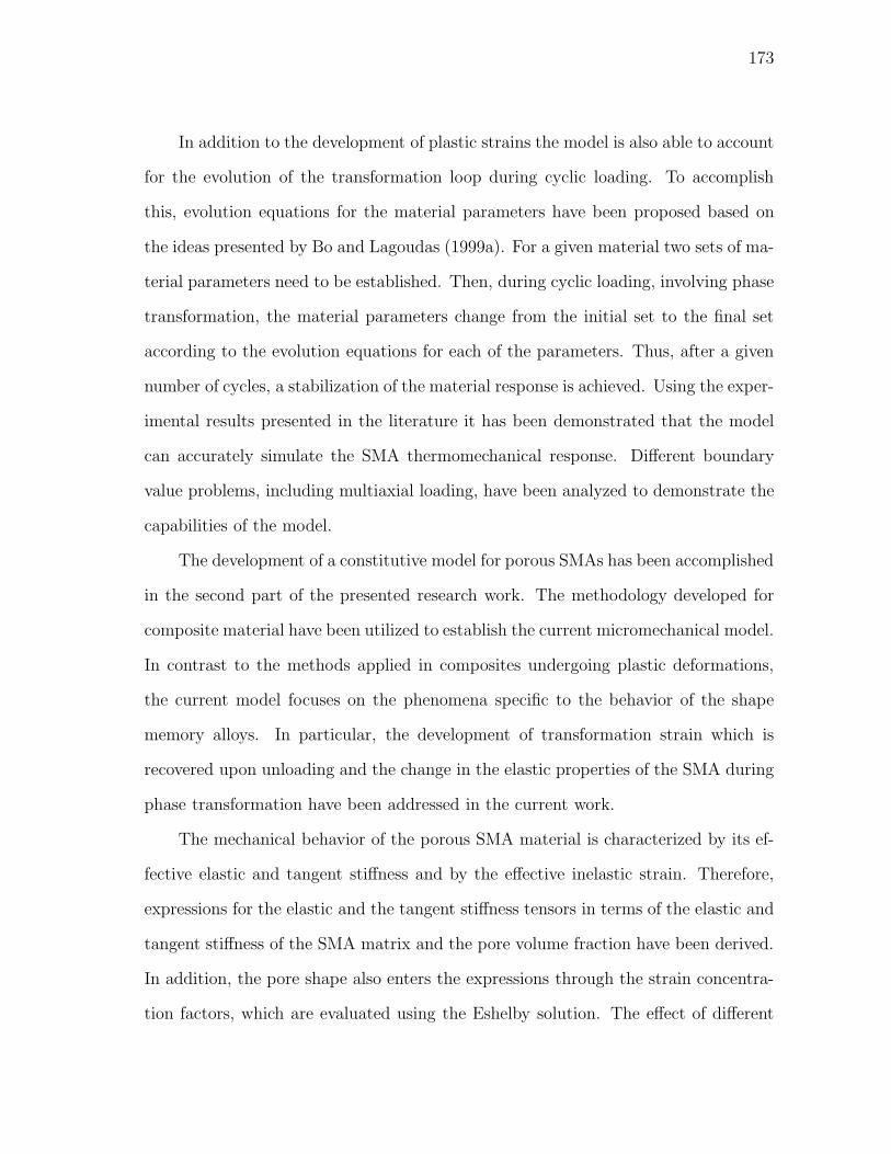
173

In addition to the development of plastic strains the model is also able to account

for the evolution of the transformation loop during cyclic loading. To accomplish

this, evolution equations for the material parameters have been proposed based on

the ideas presented by Bo and Lagoudas (1999a). For a given material two sets of ma-

terial parameters need to be established. Then, during cyclic loading, involving phase

transformation, the material parameters change from the initial set to the final set

according to the evolution equations for each of the parameters. Thus, after a given

number of cycles, a stabilization of the material response is achieved. Using the exper-

imental results presented in the literature it has been demonstrated that the model

can accurately simulate the SMA thermomechanical response. Different boundary

value problems, including multiaxial loading, have been analyzed to demonstrate the

capabilities of the model.

The development of a constitutive model for porous SMAs has been accomplished

in the second part of the presented research work. The methodology developed for

composite material have been utilized to establish the current micromechanical model.

In contrast to the methods applied in composites undergoing plastic deformations,

the current model focuses on the phenomena specific to the behavior of the shape

memory alloys. In particular, the development of transformation strain which is

recovered upon unloading and the change in the elastic properties of the SMA during

phase transformation have been addressed in the current work.

The mechanical behavior of the porous SMA material is characterized by its ef-

fective elastic and tangent stiffness and by the effective inelastic strain. Therefore,

expressions for the elastic and the tangent stiffness tensors in terms of the elastic and

tangent stiffness of the SMA matrix and the pore volume fraction have been derived.

In addition, the pore shape also enters the expressions through the strain concentra-

tion factors, which are evaluated using the Eshelby solution. The effect of different

174

pore shapes on the elastic properties of the material has been investigated. It has

been found that for the case of random orientation of ellipsoidal pores the mechanical

behavior of the material can be modeled using a spherical pore shape. However, if

a different processing technique is established which is capable of fabricating porous

SMAs with oriented porosity, the model can still be used. In the case of oriented

porosity the distribution function for the pore orientations must be given. An evolu-

tion equation for the macroscopic inelastic strain has also been derived. The effects

of different components entering the expression for the macroscopic inelastic strain

rate have been investigated and their contributions have been evaluated.

A detailed procedure for the estimation of the material parameters for both fully

dense and porous SMAs has been presented. The evaluation of the material param-

eters is given for the case of an SMA material undergoing stress-induced martensitic

phase transformation. The experimental data for two different porous NiTi alloys

has been used to estimate the material parameters used by the model. The results

of the numerical simulations have been compared with the experimental stress-strain

response of the material and it has been concluded that the model simulations are in

good agreement with the experimental observations. To demonstrate the capabilities

of the model, different boundary value problems involving multiaxial loading have

been simulated. The results for sequential torsion-compression loading of a porous

SMA bar, which is of particular interest for potential future applications, have been

presented in detail and discussed.

The numerical implementation of the constitutive model has been presented

where the methods reported by Qidwai and Lagoudas (2000a) have been utilized.

Particular attention was given to implementing the evolution of the plastic strain as

well as the evolution of the material parameters during cyclic loading. As a part of

integrating the constitutive model in a computer code with capabilities of structural

175

modeling, it has been numerically implemented in a user-supplied material subroutine

for ABAQUS.

6.2. Future Work

Based on the results of the current research effort, several topics for future research

activity can be recommended. One issue which could be addressed in future research

is the different behavior of SMAs under tension and compression. To accomplish this,

a different form of the transformation function must be specified, as shown by Qidwai

and Lagoudas (2000b). Another issue which should be addressed is the incorporation

of two-way shape memory effect into the constitutive model for the fully dense SMA.

The choice of proper tensorial variable to replace the current maximum transforma-

tion strain Hcur used in this formulation will require additional experiments. These

experiments should reveal the multiaxial effects of training and facilitate the further

development of the model. The development of plastic strain for material undergoing

incomplete transformation cycles must also be revisited. In the current model the

evolution equations for the plastic strain do not distinguish between the complete

and incomplete transformation cycles, while the experimental results suggest that

the development of plastic strain may differ for incomplete transformation cycles.

Different issues can also be addressed in the model for porous SMAs. The first

problem that should be further researched is the development of microcracks in the

porous alloys. As seen from the experimental results this is a serious problem in porous

SMAs fabricated from elemental powders. It has been observed that when subjected

to compressive loading the porous SMA specimens develop cracks and eventually

fail. Therefore, the incorporation of a damage mechanism into the constitutive model

should be considered. Another issue that may become important is the investiga-

176

tion of different orientation distribution functions for oriented porosity. Finally, the

dynamic loading of porous SMAs must also be addressed. The experiments and mod-

eling of the behavior of porous SMAs under impact loading will become important

as these materials find their applications in various energy absorption devices.

177

REFERENCES

Abeyaratne, R., Kim, S.-J., 1997. Cyclic effects in shape-memory alloys: a one-

dimensional continuum model. Int. J. Solids Struct. 34 (25), 3273–3289.

Abeyaratne, R., Kim, S.-J., Knowles, J. K., 1993. One-dimensional continuum model

for shape memory alloys. Int. J. Solids Struct. 41, 541–571.

Abeyaratne, R., Kim, S.-J., Knowles, J. K., 1994. Continuum modeling of shape

memory alloys. In: Brinson, L. C., Moran, B. (Eds.), Mechanics of Phase Trans-

formations and Shape Memory Alloys. ASME, New York, pp. 59–69.

Abeyaratne, R., Knowles, J. K., 1993. Continuum model of a thermoelastic solid

capable of undergoing phase transformation. J. Mech. Phys. Solids 41, 541–571.

Abeyaratne, R., Knowles, J. K., 1994a. Dynamics of propagating phase boundaries:

adiabatic theory for thermoelastic solids. Physica D 79, 269–288.

Abeyaratne, R., Knowles, J. K., 1994b. Dynamics of propagating phase boundaries:

Thermoelastic solids with heat conduction. Arch. Ration. Mech. Anal. 126 (3),

203–230.

Abeyaratne, R., Knowles, J. K., 1997. Impact-induced phase transitions in thermoe-

lastic solids. Phil. Trans. R. Soc. Lond. A 355, 843–867.

Achenbach, J. D., Zhu, H., 1990. Effect of interphases on micro and macromechanical

behavior of hexagonal-array fiber composites. Trans. ASME 57, 956–963.

Auricchio, F., Sacco, E., 1997. A one-dimensional model for superleastic shape-

178

memory alloys with different elastic properties between austenite and martensite.

Int. J. Non-Linear Mech. 32 (6), 1101–1114.

Auricchio, F., Taylor, R. L., Lubliner, J., 1997. Shape-memory alloys: Macromod-

elling and numerical simulations of the superelastic behavior. Computer Methods

in Applied Mechanics and Engineering 146, 281–312.

Ayers, R. A., Simske, S. J., Bateman, T. A., Petkus, A., Sachdeva, R. L. C., Gyunter,

V. E., 1999. Effects of Nitinol implant porosity on cranial bone ingrowth and ap-

position after 6 weeks. J. Biomed. Mater. Res. 45 (1), 42–47.

Benveniste, Y., 1987. A new approach to the application of Mori-Tanaka’s theory in

composite material. Mech. Mater. 6, 147–157.

Birman, V., 1997. Review of mechanics of shape memory alloy structures. Appl. Mech.

Rev. 50 (11), 629–645.

Bo, Z., Lagoudas, D. C., 1999a. Thermomechanical modeling of polycrystalline SMAs

under cyclic loading, Part III: Evolution of plastic strains and two-way memory

effect. Int. J. Eng. Sci. 37, 1141–1173.

Bo, Z., Lagoudas, D. C., 1999b. Thermomechanical modeling of polycrystalline SMAs

under cyclic loading, Part I: Theoretical derivations. Int. J. Eng. Sci. 37, 1089–1140.

Bo, Z., Lagoudas, D. C., 1999c. Thermomechanical modeling of polycrystalline SMAs

under cyclic loading, Part IV: Modeling of minor hysteresis loops. Int. J. Eng. Sci.

37, 1174–1204.

Bo, Z., Lagoudas, D. C., Miller, D., 1999. Material characterization of SMA actuators

under nonproportional thermomechanical loading. Journal of Engineering Materials

and Technology 121, 75–85.

179

Bowles, J. S., Wayman, C. M., 1972. The Bain strain, lattice correspondances and

deformations related to martensitic transformations. Metall. Trans. 3, 1113–1121.

Boyd, J. G., Lagoudas, D. C., 1994. Thermomechanical response of shape memory

composites. J. Intell. Mater. Systems Struct. 5, 333–346.

Boyd, J. G., Lagoudas, D. C., 1996. A thermodynamic constitutive model for the

shape memory materials. Part I. The monolithic shape memory alloys. Int. J. Plas-

ticity 12 (6), 805–842.

Brailovski, V., Trochu, F., 1996. Review of shape memory alloys medical applications

in Russia. Bio-Med. Mater. Eng. 6 (4), 291–298.

Budiansky, B., 1965. On the elastic moduli of some heterogeneous materials. J. Mech.

Phys. Solids 13, 223–227.

Cherkaoui, M., Sun, Q. P., Song, G. Q., 2000. Micromechanics modeling of composite

with ductile matrix and shape memory alloy reinforcement. Int. J. Solids Struct.

37, 1577–1594.

Christensen, R. M., 1991. Mechanics of Composite Materials. Krieger Publishing

Company, Malabar, FL.

Coleman, B. D., Noll, W., 1963. The thermodynamics of elastic materials with heat

conduction. Arch. Ration. Mech. Anal. 13.

Contardo, L., Guenin, G., 1990. Training and two way memory effect in Cu-Zn-Al

alloy. Acta Metall. Mater. 38 (7), 1267–1272.

De Vos, J., Aernoudt, E., Delaey, L., 1978. The crystallography of the martensitic

transformation of BCC into 9R: A generalized mathematical model. Z. Metallkde

69 (H7), 438–444.

180

DeGiorgi, V. G., Qidwai, M. A., 2001. Initial investigations into a polymer-porous

sma composite — a computational study. In: Proceedings of ASC 16th Annual

Technical Conference.

Delaey, L., 1990. Diffusionless transformations. In: Cahn, R. W., Haasen, P., Kramen,

E. J. (Eds.), Phase Transformations in Materials. Vol. 5 of Material Science and

Technologies. VCH Publishers, New York, Ch. 6, pp. 339–404.

Edelen, D. G. B., 1974. On the characterization of fluxes in nonlinear irreversible

thermodynamics. Int. J. Eng. Sci. 12, 397–411.

Entchev, P. B., Lagoudas, D. C., 2002. Modeling porous shape memory alloys using

micromechanical averaging techniques. Mech. Mater. 34 (1), 1–24.

Fischer, F. D., Oberaigner, E. R., Tanaka, K., Nishimura, F., 1998. Transformation

induced plasticity revised, an updated formulation. Int. J. Solids Struct. 35 (18),

2209–2227.

Gao, X., Huang, M., Brinson, L. C., 2000a. A multivariant micromechanical model

for SMAs. Part 1. Crystallographic issues for single crystal model. Int. J. Plasticity

16, 1345–1369.

Gao, X., Huang, M., Brinson, L. C., 2000b. A multivariant micromechanical model

for SMAs. Part 2. Polycrystal model. Int. J. Plasticity 16, 1371–1390.

Garner, L. J. Wilson, L. N., Lagoudas, D. C., Rediniotis, O. K., 2000. Development

of a shape memory alloy actuated biomimetic vehicle. Smart Mater. Struct. 9 (5),

673–683.

Gibson, L., Ashby, M., 1997. Cellular Solids, 2nd Edition. Cambridge Solid State

Science Series. Cambridge University Press, Cambridge.

181

Goncharuk, N. V., Martynova, I. F., Naidenova, O. R., Skorokhod, V. V., Solonin,

S. M., Fridman, G. R., 1992. Superelasticity and shape memory of sintered porous

titanium nickelide. Poroshk. Metall. 4, 56–60.

Green, R. J., 1972. A plasticity theory for porous solids. Int. J. Mech. Sci. 14, 215–224.

Gurson, A. L., 1977. Continuum theory of ductile rupture by void nucleation and

growth: Part I — Yield criteria and flow rules for porous ductile media. Journal of

Engineering Materials and Technology 99, 2–15.

Gyunter, V. E., Sysoliatin, P., Temerkhamor, T., 1995. Superelastic Shape Memory

Implants in Maxillofacial Surgery, Traumatology, Orthopedics, and Neurosurgery.

Tomsk University Publishing House, Tomsk, Russia.

Hashin, Z., Shtrikman, S., 1963. A variational approach to the theory of the elastic

behavior of multiphase materials. J. Mech. Phys. Solids 11, 127.

Hershey, A. V., 1954. The elasticity of an isotropic aggregate of anisotropic cubic

crystals. J. App. Mech. 21, 236–240.

Hey, J. C., Jardine, A. P., 1994. Shape memory TiNi synthesis from elemental pow-

ders. Material Science and Engineering A 188 (1-2), 291–300.

Hill, R., 1963. Elastic properties of reinforced solids: Some theoretical principles. J.

Mech. Phys. Solids 11, 357–372.

Hill, R., 1965. Continuum micromechanics of elastoplastic polycrystals. J. Mech. Phys.

Solids 13, 89–101.

HKS, 1997. ABAQUS/Standard User’s Manual. Hibbit, Karlsson & Sorensen, Inc.,

Pawtucket, RI.

182

Hutchinson, J. W., 1970. Elastic-plastic behaviour of polycrystalline metals and com-

posites. Proc. Roy. Soc. Lond. A 319, 247–272.

Ilyin, A., Dudin, M., Makarova, I., 1995. NiTi instruments for TMJ surgeries. In:

Conf. Proc. Superelastic Shape Memory Implants in Medicine. Tomsk, Russia.

Itin, V. I., Gyunter, V. E., Shabalovskaya, S. A., Sachdeva, R. L. C., 1994. Mechanical

properties and shape memory of porous Nitinol. Mater. Characterization 32, 179–

187.

Jackson, C. M., Wagner, H. J., Wasilewski, R. J., 1972. 55-nitinol—The alloy with

a memory: Its physical metallurgy, properties and applications. Tech. Rep. NASA

SP-5110, NASA, Technology Utilization Office, Washington, D.C.

Jardine, A. P., Kudva, J. M., Martin, C., Appa, K., 1996. Shape memory alloy

Ti-Ni actuators for twist control of smart wing designs. In: SPIE Proceedings of

Mathematics and Controls in Smart Structures. Vol. 2717. SPIE.

Jeong, H.-Y., Pan, J., 1995. A macroscopic constitutive law for porous solids with

pressure-sensitive matrices and its implications to plastic flow localization. Int. J.

Solids Struct. 32 (24), 3669–3691.

Kane, T. R., Likins, P. W., Levinson, D. A., 1983. Spacecraft Dynamics. McGraw-Hill

Book Company, New York.

Kato, H., Ozu, T., Hashimoto, S., Miura, S., 1999. Cyclic stress-strain response of

superelastic Cu-Al-Mn alloy single crystals. Material Science and Engineering A

264, 245–253.

Kaufman, L., Cohen, M., 1958. Martensitic transformations. In: Chalmers, B., King,

R. (Eds.), Progress in Metal Physics. Vol. 7. Pergamon Press, Oxford, pp. 165–246.

183

Kroner, E., 1958. Berechnung der elastischen konstanten des vielkristalls aus den

konstanten des einkristalls. Z. Phys. 151, 504–518.

Lagoudas, D. C., Bo, Z., 1999. Thermomechanical modeling of polycrystalline SMAs

under cyclic loading, Part II: Material characterization and experimental results

for a stable transformation cycle. Int. J. Eng. Sci. 37, 1205–1249.

Lagoudas, D. C., Bo, Z., Qidwai, M. A., 1996. A unified thermodynamic constitutive

model for SMA and finite element analysis of active metal matrix composites. Mech.

Composite Mater. Struct. 3, 153–179.

Lagoudas, D. C., Boyd, J. G., Bo, Z., 1994. Micromechanics of active composites with

SMA fibers. ASME Journal of Material Science and Technology 5, 337–347.

Lagoudas, D. C., Entchev, P. B., Qidwai, M. A., DeGiorgi, V. G., 2000a. Microme-

chanics of porous shape memory alloys. In: Redmont, J., Main, J. (Eds.), Proceed-

ings of 2000 ASME International Mechanical Engineering Congress & Exposition.

Lagoudas, D. C., Entchev, P. B., Vandygriff, E. L., Qidwai, M. A., DeGiorgi, V. G.,

2000b. Modeling of thermomechanical response of porous shape memory alloys. In:

Lynch, C. S. (Ed.), Proceedings of SPIE, Smart Structures and Materials 2000.

Active Materials: Behavior and Mechanics. Vol. 3992. SPIE.

Lagoudas, D. C., Gavazzi, A. C., Nigam, H., 1991. Elastoplastic behavior of metal

matrix composites based on incremental plasticity and the Mori-Tanaka averaging

scheme. Computational Mechanics 8, 193–203.

Lagoudas, D. C., Vandygriff, E. L., January 2002. Processing and characterization of

NiTi porous SMA by elevated pressure sintering, submitted to: J. Intell. Mater.

Systems Struct.

184

Leclercq, S., Lexcellent, C., 1996. A general macroscopic description of the thermo-

mechanical behavior of shape memory alloys. J. Mech. Phys. Solids 44 (6), 953–980.

Levitas, V. I., 1998. Thermomechanical theory of martensitic phase transformations

in inelastic materials. Int. J. Solids Struct. 35, 889–940.

Lexcellent, C., Bourbon, G., 1996. Thermodynamical model for cyclic behaviour of

Ti-Ni and Cu-Zn-Al shape memory alloys under isothermal undulated tensile tests.

Mech. Mater. 24, 59–73.

Lexcellent, C., Leclerq, S., Gabry, B., Bourbon, G., 2000. The two way shape memory

effect of shape memory alloys: an experimental study and a phenomenological

model. Int. J. Plasticity 16, 1155–1168.

Li, B.-Y., Rong, L.-J., Li, Y.-Y., 1998. Porous NiTi alloy prepared from elemental

powder sintering. J. Mater. Res. 13, 2847–2851.

Liang, C., Davidson, F., Schetky, L. M., Straub, F. K., 1996. Applications of torsional

shape memory alloy actuators for active rotor blade control — opportunities and

limitations. In: SPIE Proceedings of Mathematics and Controls in Smart Struc-

tures. Vol. 2717. SPIE.

Liang, C., Rogers, C. A., 1992. A multi-dimensional constitutive model for shape

memory alloys. Journal of Engineering Mathematics 26, 429–443.

Lim, J. T., McDowell, D. L., 1999. Mechanical behavior of a Ni-Ti shape memory

alloy under axial-torsional proportional and nonproportional loading. Journal of

Engineering Materials and Technology 121, 9–18.

Lim, T. J., McDowell, D. L., 1994. Degradation of an NiTi alloy during cyclic loading.

185

In: Proceedings of the 1994 North American Conference on Smart Structures and

Materials. SPIE.

Lu, Z. K., Weng, G. J., 2000. A two-level micromechanical theory for a shape-memory

alloy reinforced composite. Int. J. Plasticity 16, 1289–1307.

Malvern, L. E., 1969. Introduction to the Mechanics of a Continuous Medium.

Prentice-Hall, Inc., Englewood Cliffs, NJ.

Martynova, I., Skorohod, V., Solonin, S., Goncharuk, S., 1991. Shape memory and

superelasticity behaviour of porous Ti-Ni material. Journal de Physique IV , C4–

421–426.

McCormick, P. G., Liu, Y., 1994. Thermodynamic analysis of the martensitic trans-

formation in TiNi—II. Effect of transformation cycling. Acta Metall. Mater. 42 (7),

2407–2413.

Melton, K. N., 1999. General applications of SMA’s and smart materials. In: Otsuka,

K., Wayman, C. M. (Eds.), Shape Memory Alloys. Cambridge University Press,

Cambridge, Ch. 10, pp. 220–239.

Miller, D. A., Lagoudas, D. C., 2001. Influence of cold work and heat on the shape

memory effect and plastic strain development of NiTi wire actuators. Material

Science and Engineering A 308 (1–2), 161–175.

Miyazaki, S., 1999. Medical and dental applications of shape memory alloys. In: Ot-

suka, K., Wayman, C. M. (Eds.), Shape Memory Alloys. Cambridge University

Press, Cambridge, Ch. 12, pp. 267–281.

Mori, T., Tanaka, K., 1973. Average stress in matrix and average energy of materials

with misfitting inclusions. Acta Metallurgica 21, 571–574.

186

Nemat-Nasser, S., Hori, M., 1993. Micromechanics: Overall Properties of Heteroge-

neous Materials. North-Holland Series in Applied Mathematics and Mechanics, vol

37. North-Holland, Amsterdam.

Nishiyama, Z., 1978. Martensitic Transformations. Academic Press, San Diego.

Ohkata, I., Suzuki, Y., 1999. The design of shape memory alloy actuators and their

applications. In: Otsuka, K., Wayman, C. M. (Eds.), Shape Memory Alloys. Cam-

bridge University Press, Cambridge, Ch. 11, pp. 240–266.

Olson, G. B., Cohen, M., 1982. Stress assisted isothermal martensitic transformation:

Application to TRIP steels. Metall. Trans. A 13A, 1907–1914.

Otsuka, K., Wayman, C., Nakai, K., Sakamoto, H., Shimizu, K., 1976. Superelastic-

ity effects and stress-induced martensitic transformations in Cu-Al-Ni alloy. Acta

Metallurgica 24, 207–226.

Otsuka, K., Wayman, C. M., 1999a. Introduction. In: Otsuka, K., Wayman, C. M.

(Eds.), Shape Memory Alloys. Cambridge University Press, Cambridge, Ch. 1, pp.

1–26.

Otsuka, K., Wayman, C. M., 1999b. Mechanism of shape memory effect and supere-

lasticity. In: Otsuka, K., Wayman, C. M. (Eds.), Shape Memory Alloys. Cambridge

University Press, Cambridge, Ch. 2, pp. 27–48.

Patoor, E., Eberhard, A., Berveiller, M., 1988. Thermomechanical behaviour of shape

memory alloys. Arch. of Mech. 40 (5-6), 775–794.

Patoor, E., Eberhardt, A., Berveiller, M., 1994. Micromechanical modelling of the

shape memory behavior. In: Brinson, L. C., Moran, B. (Eds.), Proc. ASME

187

WAM’94: Mechanics of Phase Transformation and Shape Memory Alloys. Vol.

AMD189/PVD292. ASME.

Patoor, E., Eberhardt, A., Berveiller, M., 1996. Micromechanical modelling of su-

perelasticity in shape memory alloys. Journal de Physique IV 6, C1–277–292.

Paul, B., 1960. Prediction of elastic constants of multiphase materials. Trans. ASME

218, 36.

Perkins, J., 1974. Residual stresses and the origin of reversible (two-way) shape mem-

ory effect. Scripta Met. 8, 1469–1476.

Ponte Castaneda, P., 1996. Exact second-order estimates for the effective mechanical

properties of nonlinear composite materials. J. Mech. Phys. Solids 44 (827–862).

Qidwai, M. A., 1999. Thermomechanical constitutive modeling and numerical im-

plementation of polycrystalline shape memory alloy materials. Ph.D. thesis, Texas

A&M University.

Qidwai, M. A., Entchev, P. B., Lagoudas, D. C., DeGiorgi, V. G., 2001. Modeling

of the thermomechanical behavior of porous shape memory alloys. Int. J. Solids

Struct. 38, 8653–8671.

Qidwai, M. A., Lagoudas, D. C., 2000a. Numerical implementation of a shape memory

alloy thermomechanical constitutive model using return mapping algorithms. Int.

J. Numer. Meth. Eng. 47, 1123–1168.

Qidwai, M. A., Lagoudas, D. C., 2000b. On thermomechanics and transformation

surfaces of polycrystalline NiTi shape memory alloy material. Int. J. Plasticity 16,

1309–1343.

188

Rajagopal, K. R., Srinivasa, A. R., 1999. On the thermomechanics of shape memory

wires. Z. Agnew. Math. Phys. 50, 1–38.

Reisner, G., Werner, E. A., Fischer, F. D., 1998. Micromechanical modeling of marten-

sitic transformation in random microstructures. Int. J. Solids Struct. 35 (19), 2457–

2473.

Rengarajan, G., Kumar, R. K., Reddy, J. N., 1998. Numerical modeling of stress

induced martensitic phase transformations in shape memory alloys. Int. J. Solids

Struct. 35 (14), 1489–1513.

Rong, L., Miller, D. A., Lagoudas, D. C., 2001. Transformation behavior in a ther-

momechanically cycled Ti-Ni-Cu alloy. Metallurgical and Materials Transactions A

32 (11), 2689–2693.

Sabina, F. J., Smyshlyaev, V. P., Willis, J. R., 1993. Self-consistent analysts of waves

in a matrix-inclusion composite I. Alligned spheroidal inclusions. J. Mech. Phys.

Solids 41 (10), 1573–1588.

Sabina, F. J., Willis, J. R., 1988. A simple self-consistent analysis of wave-propagation

in particulate composites. Wave Motion 10 (2), 127–142.

Saburi, T., 1999. Ti–Ni shape memory alloys. In: Otsuka, K., Wayman, C. M. (Eds.),

Shape Memory Alloys. Cambridge University Press, Cambridge, Ch. 3, pp. 49–96.

Saburi, T., Wayman, C. M., Takata, K., Nenno, S., 1980. The shape memory mech-

anism in 18R martensitic alloys. Acta Metallurgica 28, 15–32.

Sehitoglu, H., Anderson, R., Karaman, I., Gall, K., Chumlyakov, Y., 2001. Cyclic

deformation behavior of single crystal NiTi. Material Science and Engineering A

314, 67–74.

189

Shabalovskaya, S. A., Itin, V. I., Gyunter, V. E., 1994. Porous Ni-Ti — a new material

for implants and prostheses. In: Pelton, A. R., Hodgson, D. E., Duerig, T. W.

(Eds.), Proceedings of the First International Conference on Shape Memory and

Superelastic Technologies. SMST International Committee.

Shevchenko, O. M., Gavrilyuk, G. V., Kokorin, V. V., Chernenko, V. A., 1997. Ob-

taining Fe-Ni-Co-Ti alloys having a thermoelastic martensite transformation. Pow-

der Metallurgy and Metal Ceramics 36 (1-2), 71–76.

Simo, J. C., Taylor, R. L., 1985. Consistent tangent operators for rate-independent

elastoplasticity. Computer Methods in Applied Mechanics and Engineering 48, 101–

118.

Simske, S. J., Ayers, R. A., Bateman, T. A., 1997. Porous materials for bone engi-

neering. In: Liu, D.-M., Dixit, V. (Eds.), Porous Materials for Tissue Engineering.

Vol. 250 of Materials Science Forum. Trans Tech, Uetikon-Zurich, pp. 151–182.

Smyshlyaev, V. P., Willis, J. R., Sabina, F. J., 1993a. Self-consistent analysts of

waves in a matrix-inclusion composite II. Randomly oriented spheroidal inclusions.

J. Mech. Phys. Solids 41 (10), 1589–1598.

Smyshlyaev, V. P., Willis, J. R., Sabina, F. J., 1993b. Self-consistent analysts of

waves in a matrix-inclusion composite III. A matrix containing cracks. J. Mech.

Phys. Solids 41 (12), 1809–1824.

Stalmans, R., Humbeeck, J. V., Delaey, L., 1992. The two way memory effect in

copper-based shape memory alloys—Thermodynamics and mechanisms. Acta Met-

all. Mater. 40 (11), 2921–2931.

190

Strnadel, B., Ohashi, S., Ohtsuka, H., Ishihara, T., Miyazaki, S., 1995a. Cyclic stress-

strain characteristics of Ti-Ni and Ti-Ni-Cu shape memory alloys. Material Science

and Engineering A 202, 148–156.

Strnadel, B., Ohashi, S., Ohtsuka, H., Miyazaki, S., Ishihara, T., 1995b. Effect of

mechanical cycling on the pseudoelasticity characteristics of Ti-Ni and Ti-Ni-Cu

alloys. Material Science and Engineering A 203, 187–196.

Sun, Q. P., Hwang, K. C., 1993a. Micromechanics modeling for the constitutive be-

havior of polycrystalline shape memory alloys — I. Derivation of general relations.

J. Mech. Phys. Solids 41 (1), 1–17.

Sun, Q. P., Hwang, K. C., 1993b. Micromechanics modelling for the constitutive

behavior of polycrystalline shape memory alloys — II. Study of the individual

phenomena. J. Mech. Phys. Solids 41 (1), 19–33.

Talbot, D. R. S., Willis, J. R., 1985. Variational principles for nonlinear inhomoge-

neous media. IMA J. Appl. Math. 35, 39–54.

Tanaka, K., 1986. A thermomechanical sketch of shape memory effect: One-

dimensional tensile behavior. Res Mechanica 18, 251–263.

Tanaka, K., Nishimura, F., Hayashi, T., Tobushi, H., Lexcellent, C., 1995. Phe-

nomenological analysis on subloops and cyclic behavior in shape memory alloys

under mechanical and/or thermal loads. Mechanics of Materials 19, 281–292.

Tandon, G. P., Weng, G. J., 1988. A theory of particle-reinforced plasticity. J. App.

Mech. 55, 126–135.

Tangaraj, K., Chen, Y.-C., Salama, K., 2000. Fabrication of porous NiTi shape mem-

191

ory alloy by elemental powder sintering. In: Redmont, J., Main, J. (Eds.), Proceed-

ings of 2000 ASME International Mechanical Engineering Congress & Exposition.

Truesdell, C., Noll, W., 1965. The Non-Linear Field Theories of Mechanics. Springer-

Verlag, Berlin.

Vandygriff, E. L., Lagoudas, D. C., Thangaraj, K., Chen, Y.-C., 2000. Porous shape

memory alloys, Part I: Fabrication and characterization. In: Proceedings of ASC

15th Annual Technical Conference.

Walpole, L. J., 1966. On bounds for the overall elastic moduli of inhomogeneous

systems—I. J. Mech. Phys. Solids 14, 151.

Wayman, C. M., 1983. Phase transformations, nondiffusive. In: Cahn, R. W., Haasen,

P. (Eds.), Physical Metallurgy. North-Holland Physics Publishing, New York, pp.

1031–1075.

Weng, G. J., 1984. Some elastic properties of reinforced solids, with special reference

to isotropic ones, containing spherical inclusions. Int. J. Eng. Sci. 22, 845–856.

Willis, J. R., 1883. The overall elastic response of composite-materials. J. App. Mech.

50, 1202–1209.

Willis, J. R., 1981. Variational and related methods for the overall properties of

composites. In: Yih, C. Y. (Ed.), Advances in Applied Mechanics. Academic Press,

New York, pp. 1–78.

Yi, H. C., Moore, J. J., 1990. The combustion synthesis of Ni-Ti shape memory alloys.

JOM 42, 31–35.

192

VITA

Pavlin Borissov Entchev, son of Boris E. Borissov and Stoyanka P. Borissova, was

born on September 3, 1972 in Elhovo, Bulgaria. He graduated with a silver medal from

high school in 1989 and immediately entered Belorussian State Polytechnic Academy

(BSPA) in Minsk, Belarus. Pavlin graduated from BSPA with honors and received

his M.S. degree in applied mathematics in 1994. In 1995 he accepted a position in the

Institute of Mathematics, Bulgarian Academy of Sciences. In January of 1997 Pavlin

entered the graduate program at Texas A&M University to pursue his Ph.D. degree

in Aerospace Engineering. He completed his degree in May, 2002.

Pavlin is married to Natalya A. Verkhusha and they have a son, Bogdan P. Entchev.

They can be reached at the following address:

c/o Dr. Dimitris C. Lagoudas

Department of Aerospace Engineering

Texas A&M University

College Station, TX 77843-3141

The typist for this dissertation was Pavlin Borissov Entchev.

micomechanical modeling of porous shape memory alloys

Documents