MICHPAVEUser’s Manual(Version 1.2 for DOS)

Ronald S. Harichandran Gilbert Y. Baladi

Asphalt

Base

Roadbed

1995 Michigan State University Board of Trustees

January 2000

Department of Civil and Environmental EngineeringMichigan State University

East Lansing, MI 48824-1226

MICHPAVE USER’S MANUAL

(Version 1.2 for DOS)

by

Ronald S. HarichandranAssociate Professor

and

Gilbert Y. BaladiProfessor

ii

........

.......1......1......1.......1......2.......4.....4......4.........4.......5.......5......5.....5......5...6......6.......6......6.......7......7......9....16.....18.....20......20.......20

Table of Contents1. Introduction.........................................................................................................12. Summary of Modeling and Analysis ...................................................................

2.1 Modeling of the Pavement ..................................................................2.2 Granular and Cohesive Material Models ............................................2.3 Gravity and Lateral Stresses ..............................................................2.4 Finite Element Analysis......................................................................2.5 Computation of Stresses and Strains at Layer Interfaces...................2.6 Estimated Equivalent Resilient Moduli ...............................................2.7 Fatigue and Rut Depth Prediction.......................................................

3. System Requirements.........................................................................................4. Configuring the Computer ...................................................................................

4.1 Installation Procedure ........................................................................4.2 The CONFIG.SYS File.......................................................................4.3 Required Amount of Free Memory......................................................4.4 Printing Graphics ................................................................................4.5 Running MICHPAVE for the First Time...............................................

5. Using MICHPAVE ...............................................................................................5.1 Filenames ...........................................................................................5.2 Cursor Movement and Editing Keys...................................................5.3 Title Screen ........................................................................................5.4 Main Menu..........................................................................................5.5 Data File Menus and Associated Data-Entry Forms...........................5.6 Performing Analysis ...........................................................................5.7 Plotting the Results ............................................................................5.8 Printing the Results ............................................................................

6. Problem Reporting..............................................................................................6. References..........................................................................................................

iii

.......2.......2.......3........8.........8........9....9......10....10....11.....12....12....13....13

.......14

....14

....15

......16

.....16

....17......17......18.....19.....19

......7

List of FiguresFigure 1. Resilient modulus model for granular soils .........................................................Figure 2. Resilient modulus model for cohesive soils.........................................................Figure 3. Typical finite element mesh.................................................................................Figure 4. Title screen..........................................................................................................Figure 5. Credits screen.....................................................................................................Figure 6. Main menu ..........................................................................................................Figure 7. Overview flowchart of the MICHPAVE program..................................................Figure 8. New data file menu .............................................................................................Figure 9. Data-entry form for initial data .............................................................................Figure 10. Data-entry form for fatigue life and rut depth ......................................................Figure 11. Data-entry form for layer type .............................................................................Figure 12. Data-entry form for linear elastic (type 1) material properties ............................Figure 13. Data-entry form for granular (type 2) material properties ....................................Figure 14. Data-entry form for cohesive (type 3) material properties ..................................Figure 15. Data-entry form for specifying the number of cross sections along which

results are computed ..........................................................................................Figure 16. Data-entry form for specifying the location of horizontal cross sections.............Figure 17. Data-entry form for specifying the location of vertical cross sections .................Figure 18. Data-entry form for modifying the number of elements in the vertical

direction ..............................................................................................................Figure 19. Data-entry form for modifying the number of elements in the

horizontal direction ..............................................................................................Figure 20. Typical display during computation .....................................................................Figure 21. Typical design summary.....................................................................................Figure 22. Plot menu for selecting sections .........................................................................Figure 23. Menu for plots along vertical cross sections........................................................Figure 24. Menu for plots along horizontal cross sections...................................................

List of TablesTable 1. Keypad functions within data-entry forms ...........................................................

iv

blent due to

also

arem-

of theanddran,

direc-d to bedue to

uced to

ma-

ough

the

ights.

1. Introduction

MICHPAVE is a user-friendly, non-linear finite element program for the analysis of flexipavements. The program computes displacements, stresses and strains within the pavemea single circular wheel load. Useful design information such as fatigue life and rut depth areestimated through empirical equations.

Most of MICHPAVE is written in FORTRAN 77. Graphics and screen manipulationsperformed using the FORTRAN callable GRAFMATIC graphics library, marketed by Microcopatibles Inc., 301 Prelude Drive, Silver Spring, MD 20901.

2. Summary of Modeling and Analysis

This section gives a summary of the modeling and analysis so that the user is awarecapabilities and limitations of the MICHPAVE program. Further details about the modelinganalysis, and various sensitivity studies, are given in the works by Yeh (1989), and Harichanet. al. (1989, 1990).

2.1 Modeling of the Pavement

Each layer in a pavement cross section is assumed to extend infinitely in the horizontaltions, and the last layer is assumed to be infinitely deep. All the pavement layers are assumefully bonded so that no slip occurs due to applied load. Displacements, stresses and strainsa single circular wheel load are computed. Due to the assumptions used, the problem is redan axisymmetric one.

2.2 Granular and Cohesive Material Models

The so-calledK-θ model is used to characterize the resilient moduli of granular (type 2)terials. This model is of the form

in which θ = σ1 + σ2 + σ3 = bulk stress andMR = resilient modulus, andK1 andK2 are materialproperties. For this model, log MR varies linearly with log θ as shown in Fig. 1.

The resilient modulus for cohesive soils is specified in terms of the deviatoric stress thrthe bilinear model:

This model is illustrated in Fig. 2.

2.3 Gravity and Lateral Stresses

The MICHPAVE program includes the effect of gravity and lateral stresses arising fromweight of the materials. At any location within the pavements, the vertical gravity stress (σg) iscomputed as the accumulation of the layer thicknesses multiplied by the appropriate unit weThe lateral stress is taken as

MR K1θK2=

MR

K2 K3 K1 σ1 σ3–( )–[ ], when σ1 σ3–( ) K1≤+

K2 K4 σ1 σ3–( ) K1–[ ], when σ1 σ3–( ) K1>+

=

1

input

aredbed).rey the

σh = K0σg

whereK0 = coefficient of earth pressure at rest. For granular soilsK0 = 1 − sin φ and for cohesivesoilsK0 = 1− 0.95 sinφ, whereφ = angle of internal friction.

To approximately account for “locked-in” stresses caused by compaction, the user cana value forK0 higher than the coefficient of earth pressure at rest.

2.4 Finite Element Analysis

Rectangular four-noded axisymmetric finite elements with linear interpolation functionsused in all upper layers and through the depth specified by the user for the last layer (the roaA lateral boundary is placed at a radial distance of 10a from the center of the loaded area, whea = radius of the loaded area. A default mesh is initially generated, but this may be modified buser. The default mesh has the following characteristics:

log θ

log MR

K2

1

log K1

Figure 1 Resilient modulus model for granular soils

σ1 − σ3

MR

K41K2

Figure 2 Resilient modulus model for cohesive soils

K1

K3

1

2

nyand 13 ra-

ii, isdii, is

entst fourer lay-

finitequireddaryhomo-f the fi-

eachf theprin-

inedsilient

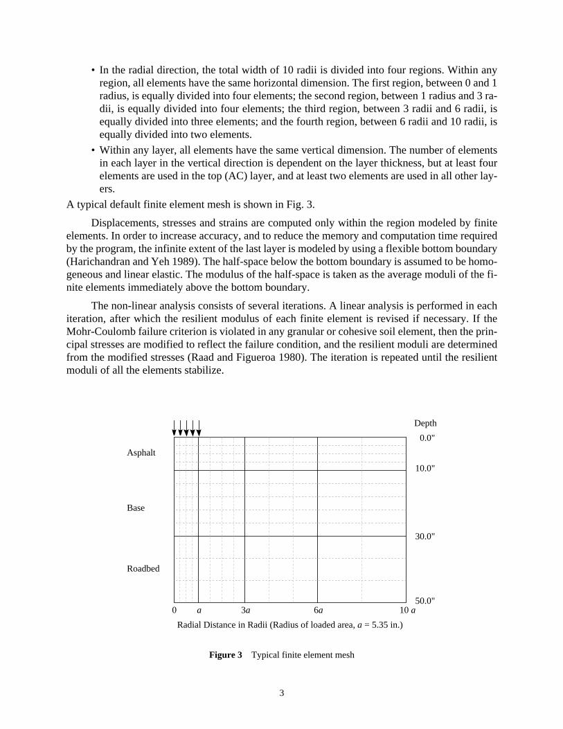
• In the radial direction, the total width of 10 radii is divided into four regions. Within aregion, all elements have the same horizontal dimension. The first region, between 0radius, is equally divided into four elements; the second region, between 1 radius anddii, is equally divided into four elements; the third region, between 3 radii and 6 radequally divided into three elements; and the fourth region, between 6 radii and 10 raequally divided into two elements.

• Within any layer, all elements have the same vertical dimension. The number of elemin each layer in the vertical direction is dependent on the layer thickness, but at leaselements are used in the top (AC) layer, and at least two elements are used in all others.

A typical default finite element mesh is shown in Fig. 3.

Displacements, stresses and strains are computed only within the region modeled byelements. In order to increase accuracy, and to reduce the memory and computation time reby the program, the infinite extent of the last layer is modeled by using a flexible bottom boun(Harichandran and Yeh 1989). The half-space below the bottom boundary is assumed to begeneous and linear elastic. The modulus of the half-space is taken as the average moduli onite elements immediately above the bottom boundary.

The non-linear analysis consists of several iterations. A linear analysis is performed initeration, after which the resilient modulus of each finite element is revised if necessary. IMohr-Coulomb failure criterion is violated in any granular or cohesive soil element, then thecipal stresses are modified to reflect the failure condition, and the resilient moduli are determfrom the modified stresses (Raad and Figueroa 1980). The iteration is repeated until the remoduli of all the elements stabilize.

0 a 3a 6a 10a

Depth

0.0"

10.0"

30.0"

50.0"

Asphalt

Base

Roadbed

Radial Distance in Radii (Radius of loaded area,a = 5.35 in.)

Figure 3 Typical finite element mesh

3

ns areed es-

ments

olationce. Ifts arethen

achusingcom-

ed 2:1

sed ast thepave-ts withypes ofber of, per-essivemper-

rss run-

gly

2.5 Computation of Stresses and Strains at Layer Interfaces

For the interpolation functions used in the finite element approach, stresses and straimost accurate at the center of elements. The following techniques are used to obtain improvtimates of some stresses and strains at layer interfaces:

• The vertical stress is obtained from the vertical stresses at the center of the two eleabove and the two elements below the interface by using cubic interpolation.

• The radial, tangential and shear stresses and vertical strain are obtained using extrapof the corresponding quantity at the center of the elements on one side of the interfaat least four elements are available then cubic extrapolation is used, if three elemenavailable then quadratic extrapolation is used, and if only two elements are availablelinear extrapolation is used.

2.6 Estimated Equivalent Resilient Moduli

At the end of the analysis, MICHPAVE outputs an equivalent resilient modulus for epavement layer. These equivalent moduli may be useful if further analyses is to be performedother programs that assume linear elastic materials. The equivalent moduli for each layer isputed as the average of the moduli of the finite elements in that layer that lie within an assumload distribution zone (Harichandran et. al. 1990).

2.7 Fatigue and Rut Depth Prediction

Results from the non-linear mechanistic analysis, together with other parameters, are uinput to two performance models derived on the basis of field data (Baladi 1989), to predicfatigue life and rut depth. These performance models are currently restricted to three-layerments with asphalt concrete (AC) surface, base and roadbed soil, and four-layer pavemenAC surface, base, subbase and roadbed soil. Fatigue life and rut depth estimates for other tsections may be meaningless. The models relate the fatigue life and rut depth to the numequivalent 18-kip single-axle loads, surface deflection, moduli and thicknesses of the layerscent air voids in the asphalt, tensile strain at the bottom of the asphalt layer, average comprstrain in the asphalt layer, kinematic viscosity of the asphalt binder, and average annual air teature.

3. System Requirements

The MICHPAVE program was originally written for IBM compatible personal computerunning under DOS. Presently it is also available for Sun and Hewlett-Packard workstationning under UNIX. For DOS systems, the following hardware and software are required:

• PC-DOS or MS-DOS version 3.0 or higher

• 640 KB of random access memory (RAM)

• A hard disk

• A color graphics adapter (CGA, EGA or VGA) and compatible monitor

Although not strictly required for the use of the program, the following hardware is stronrecommended:

4

d if a

ard.

andnt will

lledvers the

press-St elim-

oryr pro-mande re-

yed:

mes-

if theICH-that

• A math co-processor (8087, 80287 or 80387). Running time will be greatly increasemath co-processor is not installed.

• A printer for obtaining hardcopies of plots and output.

4. Configuring the Computer

4.1 Installation Procedure

The MICHPAVE program is initially supplied a diskettes. To install the program on a hdisk, first make a subdirectory to hold the program (e.g.,MD \MPAVE), change to this directory (e.gCD \MPAVE), insert the diskette in drive A:, and typeCOPY A:*.* .

4.2 The CONFIG.SYS File

In the root directory, there is a file named CONFIG.SYS which configures the PC systemloads any requested device drivers when the computer is turned on. The following statemeneed to be added to the CONFIG.SYS file, if it does not already exist:FILES=20

The MICHPAVE program uses a FORTRAN callable graphics package caGRAFMATIC. Unfortunately, this package is not compatible with the ANSI.SYS device driused by some other programs for screen manipulations. Thus, if the CONFIG.SYS file hastatementDEVICE=ANSI.SYS

then this statement will need to be removed and the computer re-booted (by simultaneouslying theCTRL, ALT andDEL keys) before running MICHPAVE. If available, use of an ANSI.SYcompatible device driver that can be unloaded from memory on demand is convenient since iinates the need to re-boot the computer.

4.3 Required Amount of Free Memory

The MICHPAVE program requires about 515 KB of free memory to run. DOS and memresident programs (such as SIDEKICK) reduce the amount of free memory for use by othegrams. The amount of free memory available can be checked by using the DOS comCHKDSK. If there is insufficient free memory, then memory resident programs will need to bmoved before running MICHPAVE.

If there is insufficient memory to load the program, the following message will be displaProgram too big to fit in memory.

Sometimes the program may load into memory without any problem, but the following errorsage may be displayed during computations:Run-time error F6700:-heap space limit exceeded.

This also indicates that there is insufficient free memory.

4.4 Printing Graphics

Graphic screens produced by MICHPAVE can be dumped onto an attached printerDOS command GRAPHICS.COM is issued after the computer is turned on and before MPAVE is used. It may be convenient to include the command in the AUTOEXEC.BAT file so

5

een to

nningade

er isE so

ems.

theally

BM-entry

nsedprop-

be-132

ps inof in-h data-

neces-tofault

cur-t and

it is issued every time the computer is turned on. To download graphics that are on the scrthe printer simply press theSHIFT andPrScr keys simultaneously.

4.5 Running MICHPAVE for the First Time

To run MICHPAVE simply type:MICHPAVE. When running for the first time, the programwill request the following information about the computer system:Which graphics adapter and monitor do you have (MONO/CGA/EGA)?Is your computer strictly IBM compatible (Y/N)?Is your printer EPSON or EPSON compatible (Y/N)?

The response to the above prompts are stored in a file named SYSTEM.DAT. When ruMICHPAVE subsequently, the system information is read from this file. In case a mistake is mwhen specifying this information, or if the graphics adapter in the computer or the printchanged at a later time, the file SYSTEM.DAT should be deleted before running MICHPAVthat it will prompt again for a description of the new hardware.

The graphics resolution for EGA systems will be substantially higher than for CGA systFor VGA systems, specify EGA.

If the computer is not strictly IBM compatible, then problems may be encountered withdata-entry forms due to incompatibility with the graphics software, if the computer had originbeen specified as being fully IBM compatible. By defining the computer to be not strictly Icompatible MICHPAVE can still be used, but some of the color used to enhance the dataforms will be lost.

For EPSON compatible printers MICHPAVE automatically sets the print mode to condewhen printing the output after an analysis, so that the 132-column wide output file is printederly. If the printer is not EPSON compatible, then its print mode will need to be set externallyfore printing the output. For an EPSON printer with a wide carriage capable of printingcharacters per line in normal mode, specify the printer to be non-EPSON compatible.

5. Using MICHPAVE

MICHPAVE is designed to be user-friendly. Menus are used to perform the required stepavement analysis, and data-entry forms facilitate data input. In addition, extensive checkingput data is performed and appropriate error messages are displayed upon completion of eacentry form.

5.1 Filenames

The names of files in which the data and results are saved may include a pathname ifsary (e.g., A:I-96.DAT to save the file I-96.DAT on the diskette in drive A:, \JOB1\I-96.DATsave the file in subdirectory JOB1, etc.). If no path is specified, the file will be saved in the desubdirectory.

5.2 Cursor Movement and Editing Keys

The data-entry forms have several fields into which data is typed. The field in which thesor resides is highlighted on IBM compatible systems. The functions of the cursor movemenediting keys within a data-entry form are described in Table 1.

6

menu.

y be

7.

ec-.

beenese

sign.

verticalefore.PLT

5.3 Title Screen

When MICHPAVE is loaded the title screen shown in Fig. 4 is displayed. Pressing theF1keydisplays the credits screen shown in Fig. 5, while pressing any other key displays the main

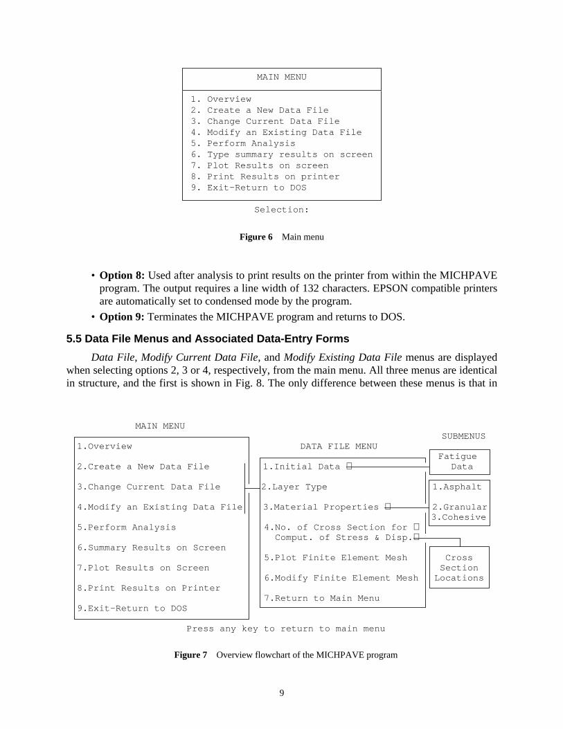
5.4 Main Menu

The main menu is shown in Fig. 6. Any one of the nine options shown on the menu maselected by typing a number from 1 to 9. These options are described below:

• Option 1: Displays the overview flowchart of the MICHPAVE program shown in Fig.

• Option 2: Used to input data relating to a new pavement analysis problem.

• Option 3: Used to change data for the problem currently being worked on.

• Option 4: Used to read the data from a previously defined problem, and modify it if nessary. The name of the file in which the previous data was saved will be requested

• Option 5: Performs non-linear finite element analysis after all the required data hasspecified. MICHPAVE creates two files named V.PLT and R.PLT after an analysis. Thfiles contain results used in subsequent plots.

• Option 6: Displays a summary screen containing the results commonly used in deThis option can only be used following an analysis.

• Option 7: Plots displacements, stresses and strains on the screen along requestedand horizontal sections. This option is normally selected after an analysis. If chosen ban analysis, the results from the previous analysis are plotted if the files V.PLT and Rhave not been erased.

TABLE 1 KEYPAD FUNCTIONS WITHIN DATA-ENTRY FORMS

KEY Function

Return/Enter Move cursor to next field

Tab Move cursor to next field on the right

Shift Tab Move cursor to previous field on the left

Home Move cursor to first field in the form

End Move cursor to last field in the form

↑ or PgUp Move cursor to field above current one

↓ or PgDn Move cursor to field below current one

Backspace Delete character before cursor

Del Delete character at cursor

Ins Insert space at cursor

→ Move cursor one space to the right

← Move cursor one space to the left

F1Check validity of entries in each field and save data. If someof the data is invalid prompts will be issued for corrections.

EscDiscards any changes made on the current screen and returnto previous screen.

7

Version 1.2MICHPAVE

Nonlinear Finite Element Programfor Analysis of Flexible Pavements

Developed forMichigan Department of Transportation

by

Dept. of Civil & Environmental EngineeringMichigan State University

East Lansing, MI 48824-1226

For further information, call:(517) 355-5107

F1 to list credits Press any key to start

Figure 4 Title screen

MICHPAVE Version 1.2April 1994

Conceptual Development by:Ronald S. Harichandran, Gilbert Y. Baladi,

and Ming-Shan Yeh

Ported to UNIX by:Ronald S. Harichandran and Baoyan Wu

Development of Version 1.0 for DOS Funded by:Michigan Department of Transportation

Acknowledgement:Various State Highway Agencies provided the data

used to develop the rut and fatigue models

Press any key to start

Figure 5 Credits screen

8

Enters

nticalhat in

• Option 8: Used after analysis to print results on the printer from within the MICHPAVprogram. The output requires a line width of 132 characters. EPSON compatible priare automatically set to condensed mode by the program.

• Option 9: Terminates the MICHPAVE program and returns to DOS.

5.5 Data File Menus and Associated Data-Entry Forms

Data File, Modify Current Data File, andModify Existing Data Filemenus are displayedwhen selecting options 2, 3 or 4, respectively, from the main menu. All three menus are idein structure, and the first is shown in Fig. 8. The only difference between these menus is t

MAIN MENU

1. Overview2. Create a New Data File3. Change Current Data File4. Modify an Existing Data File5. Perform Analysis6. Type summary results on screen7. Plot Results on screen8. Print Results on printer9. Exit-Return to DOS

Selection:

Figure 6 Main menu

MAIN MENU SUBMENUS1.Overview DATA FILE MENU

Fatigue2.Create a New Data File 1.Initial Data Data

3.Change Current Data File 2.Layer Type 1.Asphalt

4.Modify an Existing Data File 3.Material Properties 2.Granular3.Cohesive

5.Perform Analysis 4.No. of Cross Section for Comput. of Stress & Disp.

6.Summary Results on Screen5.Plot Finite Element Mesh Cross

7.Plot Results on Screen Section6.Modify Finite Element Mesh Locations

8.Print Results on Printer7.Return to Main Menu

9.Exit-Return to DOS

Press any key to return to main menu

Figure 7 Overview flowchart of the MICHPAVE program

9

. It is

mesover-

bold

those used for modifying data files, existing data is modified instead of specifying new datarecommended that the options in the data file menu be followed in sequence.

When modifying an existing file it is mandatory to first use option 1 and specify new nafor the required filenames, or to indicate that the input and output files used earlier should bewritten. The other options may be performed in any sequence.

5.5.1 Option 1: Initial, fatigue life and rut depth data

This option displays the data-entry form shown in Fig. 9 (typical data is also shown intypeface).

DATA FILE MENU

1. Initial Data (Load, No. of Layers, Output Filename, etc.)

2. Specify Layer Type

3. Specify Material Properties

4. Specify Cross Sections for Computation of Stresses & Displacements

5. Plot Finite Element Mesh

6. Modify Finite Element Mesh

7. Return to Main Menu

Selection:

Figure 8 New data file menu

INITIAL DATA

1. Filename to Save Data to: I-96.dat

2. Filename to Output Results to: I-96.out

3. Title: Section of I-96 at Williamston

4. Number of Layers: 3 (max. 6)

5. Wheel Load: 9000.0 (lb.)

6. Tire Pressure: 100.00 (psi)

7. Fatigue Life & Rut Depth Computation Required (Y/N)? Y

Figure 9 Data-entry form for initial data

10

is

.or. It

ay-

s arehese

d soil(Bal-

ot betigue

ions.es.

below:

ave-

The data that should be entered into the fields are described below:

1. Filename to Save Data to:All data that is entered in this and other forms is stored in thfile. The data may be recovered at a later time and modified if necessary.

2. Filename to Output Results to:The output from the analysis will be directed to this fileThe output is in standard ASCII form and may be viewed or edited using any text editshould be noted however that a line width of 132 characters is used for the output.

3. Title: This is a description of the current job for identification purposes.

4. Number of Layers: The number of layers in the pavement section. A maximum of six lers are permitted. Note that the roadbed soil (subgrade) is counted as one layer.

5. Wheel Load: Equal to half the axle load in pounds.

6. Tire Pressure:The pressure in the truck tire in psi.

7. Fatigue Life & Rut Depth Computation Required (Y/N)? The user should respond witha Y if fatigue life and rut depth in the section are to be estimated. Empirical expressionused to relate the fatigue life and rut depth to results from the mechanistic analysis. Trelations are currently valid only for three-layer pavements with AC, base and roadbelayers, and for four-layer pavements with AC, base, subbase and roadbed soil layersadi 1989). Fatigue life and rut depth estimates for other pavement sections may nmeaningful. The rut depth is estimated for the number of load repetitions causing fafailure of the pavement.

Answering in the affirmative to question 7 in theInitial Data form displays the data-entryform shown in Fig. 10, which is used to enter data for the fatigue life and rut depth calculatThe data table below the form shows typical kinematic viscosities for different asphalt grad

The data that should be entered into the fatigue life and rut depth form are described

1. Average Annual Temperature:The average annual air temperature expected at the pment location.

FATIGUE LIFE & RUT DEPTH DATA

1. Average Annual Temperature: 77.00 (Fahrenheit)

2. Percent Air Voids in Asphalt Mix (1,3.5, etc.): 3.00

3. Kinematic Viscosity: 270.00 (centistoke)

Asphalt Grade Typical Kinematic Viscosity (centistokes)

AC 2.5 159 AC 5.0 212 AC 10 270

Figure 10 Data-entry form for fatigue life and rut depth

11

ed

1, 2. As-terials

cify all

and 3.

yers,essureeral

2. Percent Air Voids in Asphalt Mix: The percent air voids in the asphalt mix as expectin the field.

3. Kinematic Viscosity: The kinematic viscosity of the asphalt binder.

5.5.2 Option 2: Layer type

The type of material used for each layer in the pavement section is identified by typingor 3 for asphalt, granular or cohesive soil layers, respectively, into the form shown in Fig. 11phalt is treated as a linear elastic material in the analysis. Lime asphalt or cement treated mamay be specified as type 3. To perform a linear analysis of the entire pavement section spelayers to be of type 1. Specifying types 2 or 3 implies non-linear analysis.

5.5.3 Option 3: Material properties

Three different sets of material properties are required for the three material types 1, 2

Properties for layers with asphalt or linear elastic materials, including the names of the lathicknesses, resilient moduli, Poisson's ratios, densities, and coefficients of lateral earth pr(K0), are specified in the form shown in Fig. 12. For compacted layers, the “locked-in” latstresses can be approximately accounted for by specifying a relatively large value forK0 (e.g., larg-er than 0.4).

LAYER TYPE

1 Asphalt or Linear; 2 Granular; 3 Cohesive

Layer number (from top) Type (1,2, or 3)

1 1

2 2

3 3

Figure 11 Data-entry form for layer type

ASPHALT MATERIAL PROPERTIES

Layer Name of Layer Thickness Modulus Poisson's Density Ko (inches) (psi) Ratio (lb/cu.ft)

1 Asphalt 10.0 500000.0 .35 150.0 .40

Note: Typical values for Ko are .4 (undisturbed) to 3 (heavily compacted layer)

Figure 12 Data-entry form for linear elastic (type 1) material properties

12

nts of

rs

nts of

ame-

Properties for granular layers, including the names of the layers, thicknesses, coefficielateral earth pressure (K0), K1 andK2 parameters, Poisson's ratios (µ), cohesions, friction angles(φ), and densities are specified in the form shown in Fig. 13. Typical values of the parameteK1andK2 for a variety of granular soils are displayed in the table below the form.

Properties for cohesive layers, including the names of the layers, thicknesses, coefficielateral earth pressure (K0), K1, K2, K3 andK4 parameters, Poisson’s ratios (µ), cohesions, frictionangles (φ), and densities are specified in the form shown in Fig. 14. Typical values of the par

GRANULAR MATERIAL PROPERTIES

Layer Name of Layer Thick. Ko K1 K2 µ Cohesion φ Density (in.) (psi) (psf) (degree) (pcf)

2 Base 20.0 .40 9000.0 .35 .40 .0 30.0 120.0

Resilient Modulus = K1 * ( σ1 + σ2 + σ3)**K2

Material Type K1 K2 Material Type K1 K2

Silty Sand 1620 .62 Sand/Aggregate 4350 .59 Sand Gravel 4480 .53 Partially Crushed Gravel 5967 .52 Crushed Gravel 7210 .45 Limerock 14030 .40 Slag 24250 .37

Warning: Values of K1 are dependent on the degree of saturation

Figure 13 Data-entry form for granular (type 2) material properties

COHESIVE MATERIAL PROPERTIES

Layer Name of Thick. Ko K1 K2 K3 K4 µ Coh. φ Dens. Layer (in.) (psi) (psi) (psf) (deg) (pcf)

3 Roadbed 20.0 .40 6.0 3020.0 1110.0 178. .45 800.0 .0 120.0

Note:- 1. Typical values for K1, K2, K3, K4: K1 = 6 psi, K2 = 3020 psi, K3 = 1110, K4 = 178 2. Resilient Modulus = K2 + K3 * [K1 - ( σ1 - σ3)]; K1 > ( σ1 - σ3) Resilient Modulus = K2 + K4 * [( σ1 - σ3) - k1]; K1 < ( σ1 - σ3) 3. µ = Poisson's Ratio 0 < µ < .5 4. Layer 3 actually semi-infinite, but thickness controls depth to which displacements/stresses are computed.

Figure 14 Data-entry form for cohesive (type 3) material properties

13

lished

ls theo 12" is

ections-entry

formectionied atost ac-

ons ofeach

r table

d

tersK1, K2, K3 andK4 are given in the notes. These parameters have currently not been estabwidely for different cohesive soils.

It should be noted that the thickness specified for the last layer (roadbed soil) controdepth to which displacements, stresses, and strains are computed. A thickness of about 6" trecommended. For analysis, the last layer is actually considered to be semi-infinite.

5.5.4 Option 4: Cross sections for computation of results

Displacements, stresses and strains are computed along horizontal and vertical cross sspecified by the user. The number of horizontal and vertical sections are specified in the dataform shown in Fig. 15. At least one vertical section must be used.

The depths at which the horizontal sections are located are specified in the data-entryshown in Fig. 16. To aid in these specifications the thickness of each layer in the pavement sis displayed in the upper table on the right. Although the horizontal sections may be specifany depth within the pavement, in the finite element method some stresses and strains are mcurately computed at the center of elements. Thus, best results will be obtained if the locatithe horizontal sections correspond to the mid-depths of elements. Optimal locations withinlayer, corresponding to the mid-depths of the elements in that layer, are shown in the lowe

CROSS SECTION SPECIFICATION MENU

Number of Horizontal Sections: 4

Number of Vertical Sections: 2

Figure 15 Data-entry form for specifying the number of cross sections along which results are compute

HORIZONTAL SECTION SPECIFICATIONS Layer Name Thick (in.)

1. Asphalt 10.0 Section No. Depth (inches) 2. Base 20.0

3. Subgrade 20.0 1 .00

2 10.00Optimal Locations for stress & strain

3 28.00 Layer Depths(in.)

4 33.30 1. 1.3, 3.8, 6.3, 8.8

2. 12.0, 16.0, 20.0, 24.0, 28.0

3. 33.3, 40.0, 46.7

Figure 16 Data-entry form for specifying the location of horizontal cross sections

14

t eachthe bot-

-entry

mentre mostationsts are

ents,nded

a

d thethe

allyccura-

tionsin Fig.num-e ver-mum

on the right. Nevertheless, it is strongly recommended that horizontal sections be specified alayer interface. Note that the most critical stresses are compression at the top and tension attom of the AC surface, and compression at the top of the roadbed soil.

The radial distances at which the vertical sections are located are specified in the dataform shown in Fig. 17. The first section must be located at the center of the loaded area (r = 0").Although the other vertical sections may be specified at any radial distance within the pavemodeled by finite elements (0 to 10 radii of the loaded area), some stresses and strains aaccurately computed at the center of elements. Thus, best results will be obtained if the locof the vertical sections correspond to the middle of an element. In MICHPAVE, the elemengrouped into three regions in the radial direction, from 0 toa, a to 3a, 3a to 6a, and 6a to 10a, wherea = radius of loaded area. Optimal radial locations, corresponding to the middle of the elemare shown in the table on the right. Due to edge effects of the right boundary, it is recommethat vertical section not be specified in the last region from 6a to 10a. The radius of the loaded areis shown in the note below the tables.

5.5.5 Option 5: Plot finite element mesh

This option plots the current finite element mesh on the screen. The loaded region anradius of the loaded area,a, are also shown. (Fig. 3 shows a typical finite element mesh formesh parameters given in bold typeface in Figs. 18 and 19.)

5.5.6 Option 6: Modify finite element mesh

This option is used to modify the current finite element mesh. MICHPAVE automaticgenerates a default mesh that should be sufficient for most purposes. However, for greater acy, or for unusual situations, the user may wish to modify the default mesh. Memory limitamay, however, preclude the use of a very fine (large) mesh. First, the data-entry form shown18 is displayed for modifying the number of elements in the vertical direction, and the currentber of elements within each layer are shown. All elements within a given layer have the samtical dimension. For the default number of elements in the horizontal direction (13), the maxinumber of elements in the vertical direction are currently limited to 24.

VERTICAL SECTION SPECIFICATIONS Optimal Locations for stress & strain Region Radial Distance(in.)

Section Rad. Dist.(in.) 0 - a .7, 2.0, 3.3, 4.7

1 .00 a - 3a 6.7, 9.4, 12.0, 14.7

2 4.7 3a - 6a 18.7, 24.1, 29.4

Note: 1. Radius of Loaded area a = 5.35 inches 2. Optimal points for current finite element mesh

Figure 17 Data-entry form for specifying the location of vertical cross sections

15

d forents.

(force ofand onitera-uiringnd theal dis-

After the required changes are made, the data-entry form shown in Fig. 19 is displayemodifying the number of elements in the horizontal direction, and the current number of elemin the ranges 0 toa, a to 3a, 3a to 6a, and 6a to 10a, wherea = radius of loaded area, are shownAll elements within a given range have the same horizontal dimension.

5.6 Performing Analysis

The analysis portion of MICHPAVE consists of an initialization part, several iterationsnon-linear material), and a concluding part. The number of iterations required for convergenthe non-linear solution depends on the properties of the pavement section being analyzed,the magnitude of the wheel load. Weaker sections will in general require a larger number oftions for convergence. The maximum number of iterations allowed is 25. Pavements reqmore iterations than this will probably be too weak to be practicable. The stage of analysis atime required for the previous stages are displayed on the screen during computation. A typic

MODIFY NUMBER OF ELEMENTS IN VERTICAL DIRECTION

Layer Thickness Number of Elements

1. Asphalt 10.0 4

2. Base 20.0 5

3. Subgrade 20.0 3

Total vertical elements ≤ 24; when total hori. elements = 13 (default value).

Figure 18 Data-entry form for modifying the number of elements in the vertical direction

MODIFY NUMBER OF ELEMENTS IN HORIZONTAL DIRECTION

Range (a: contact radius) Number of Elements

1. R = 0 - a 4

2. R = a - 3a 4

3. R = 3a - 6a 3

4. R = 6a - 10a 2

Note: Radius of loaded area a = 5.35 inches

Figure 19 Data-entry form for modifying the number of elements in the horizontal direction

16

oces-

rma-ressivenum-

the fa-tableilures thatg and

play is shown in Fig. 20 (the times shown were obtained on a PC with 80286 and 80287 prsors).

After the analysis is completed a design summary is displayed, showing key design infotion such as the maximum tensile strain at the bottom of the asphalt layer, the average compstrain in the asphalt layer, the maximum compressive strain at the top of the roadbed soil, theber of equivalent standard axle loads required to cause fatigue failure, and the rut depth attigue life. A typical summary is shown in Fig. 21. The caution statement at the bottom of theis a warning that if the estimated fatigue life is greater than 20 million load repetitions, then fawould most probably occur due to thermal cracking rather than fatigue. The implication here i20 million ESAL will span a period of greater than 15 to 20 years. Hence asphalt hardeninblock cracking should be considered.

CALCULATION IN PROGRESS - PLEASE WAIT

Initialization (Completion time = 0 min 24 sec)

Iteration 1 (Completion time = 0 min 50 sec)

Iteration 2 (Completion time = 1 min 2 sec)

Conclusion (Completion time = 0 min 24 sec)

Total computation time = 2 min 40 sec

Press any key to continue

Figure 20 Typical display during computation

DESIGN SUMMARY

1. Max. Tensile strain in the asphalt layer = 1.116e-04

2. Average compressive strain in the asphalt layer = 8.947e-05

3. Max. compressive strain at top of subgrade = 1.112e-04

4. Fatigue life of asphalt pavement = 1.204e+08 ESAL

5. Total expected rut depth of the pavement = 1.885e-01 (in)

6. Expected rut depth in the asphalt course = 6.966e-02 (in)

7. Expected rut depth in the base and/or subbase course = 9.097e-02 (in)

8. Expected rut depth in the roadbed soil = 2.791e-02 (in)

Caution: Thermal cracking of the pavement needs to be evaluated

Figure 21 Typical design summary

17

te newic vis-e Fa-nged.usingt whichform-esiredagain.

hso thathori-2.

tions.antitiesplotted

l sec-re com-rouped

Following the summary results the following questions will be asked:Output fatigue life and summary results to printer (Y/N)?Recompute fatigue life and rut depth with different data (Y/N)?

These questions allow the user to output the summary results to the printer, and to recompufatigue life and rut depth estimates for different values of annual temperature, and kinematcosity of the asphalt binder. Answering in the affirmative to the second question displays thtigue Life and Rut Depth data-entry form (see Fig. 10) on which these input data may be chaNote that the re-estimation of the fatigue life and rut depth for changes in this data is doneempirical equations, and does not require a re-analysis. Also note that this is the only stage afatigue life and rut depth may be estimated for the pavement for new input data, without pering a re-analysis. If the fatigue life and rut depth are not recomputed at this stage, but are dat a later time for the same pavement section, then the analysis will need to be performedAll calculations of the fatigue life and rut depth will be saved in the output file.

5.7 Plotting the Results

After an analysis, the results may be plotted. When this option is chosenbeforean analysis,the results from thepreviousanalysis will be plotted provided the files V.PLT and R.PLT whiccontain the data for plots have not been deleted. Every analysis overwrites these plot files,only one set is maintained at any given time. Results may be plotted along the vertical andzontal sections previously specified by the user by selecting from the menu shown in Fig. 2

The menu in Fig. 23 is used to select the quantities that may be plotted along vertical secThe vertical compressive and radial tensile stresses and the radial tensile strains are the quthat are commonly plotted. These are grouped together, and other quantities that may beare grouped below them.

The menu in Fig. 24 is used to select the quantities that may be plotted along horizontations. The vertical compressive stresses and the vertical deflections are the quantities that amonly plotted. These are grouped together, and other quantities that may be plotted are gbelow them.

PLOT RESULTS MENU

1. Plot results at vertical sections

2. Plot results at horizontal sections

3. Return to main menu

Selection:

Figure 22 Plot menu for selecting sections

18

PLOT RESULTS AT VERTICAL SECTIONS MENU

1. Compressive (Vertical) stresses

2. Tensile (Radial) stresses

3. Tensile (Radial) strains

4. Compressive (Vertical) strains

5. Vertical deflections

6. Radial displacements

7. Shear stresses

8. Tangential stresses

9. Return to plot results menu

Selection:

Figure 23 Menu for plots along vertical cross sections

PLOT RESULTS AT HORIZONTAL SECTIONS MENU

1. Compressive (Vertical) stresses

2. Vertical deflections

3. Tensile (Radial) stresses

4. Tensile (Radial) strains

5. Compressive (Vertical) strains

6. Radial displacements

7. Shear stresses

8. Tangential stresses

9. Return to plot results menu

Selection:

Figure 24 Menu for plots along horizontal cross sections

19

with-hine 132ensedy the

hey time

mply

g theions is

termi-

du.

pave-

r the

lfill-

5.8 Printing the Results

The output from the analysis stored in the file specified by the user may be printed fromin MICHPAVE, or from the DOS environment. When the printing option is chosen from witMICHPAVE, EPSON compatible printers are automatically set to condensed mode so that thcharacter wide lines in the output file can be printed. For printers whose code for setting condmode differs from that used for EPSON printers, the print mode should be set externally buser. The DOS commandMODE, LPT1:132 can be used to set the line width of the printer on tparallel port LPT1 to 132 characters. It may be desirable to create a batch file to do this everbefore running MICHPAVE, and to reset the printer upon exit from MICHPAVE.

To print from the DOS environment, set the printer width as outlined above, and then siuse the PRINT command.

Any text editor can also be used to view the ASCII output files.

6. Problem Reporting

Although MICHPAVE has been tested quite extensively, it is possible that errors causinprogram to terminate abnormally may still be encountered if a haphazard sequence of optused. To report a problem, note down the number and message displayed when the programnates abnormally, and send it along with a diskette containing the input data file to:

Dr. Ronald Harichandran or Dr. Gilbert BaladiDepartment of Civil & Environmental EngineeringMichigan State UniversityEast Lansing, MI 48824-1226

Alternatively, report the problem by e-mail to harichan@egr.msu.edu or baladi@egr.msu.e

References

Baladi, G.Y. (1989). “Fatigue life and permanent deformation characteristics of asphalt concrete mixes,”Transporta-tion Research Record, 1227, 75–86.

Harichandran, R.S., Baladi, G. Y., and Yeh, M-S. (1989). “Development of a computer program for design ofment systems consisting of layers of bound and unbound materials,”Report No. FHWA-MI-RD-89-02, Michi-gan Department of Transportation, Lansing, Michigan.

Harichandran, R.S. and Yeh, M-S. (1989). “Flexible boundary in finite element analysis of pavements,”Transporta-tion Research Record, 1207, 50–60.

Harichandran, R. S., Yeh, M-S., and Baladi, G. Y. (1990). “MICH-PAVE: A nonlinear finite element program foanalysis of flexible pavements.”Transportation Research Record, 1286, 123–131.

Raad, L., and Figueroa, J. L. (1980). “Load response of transportation support system,”Journal of Transportation En-gineering, ASCE, 106, 111–128.

Yeh, M-S. (1989). “Nonlinear finite element analysis of flexible pavements,” dissertation submitted in partial fument of the degree of Doctor of Philosophy, Michigan State University, East Lansing, Michigan.

20