michael j. alexander constraint management of reduced...

Michael J. AlexanderPropulsion Systems Research Lab,

General Motors Technical Center,

330500 Mound Road,

Warren, MI 48090

e-mail: [email protected]

James T. AllisonDepartment of Industrial and Enterprise Systems

Engineering,

University of Illinois at Urbana-Champaign,

117 Transportation Building MC-238,

104 S. Mathews Avenue,

Urbana, IL 61801


Panos Y. PapalambrosDepartment of Mechanical Engineering,

University of Michigan,

3200 EECS c=o 2250 G.G. Brown,

2350 Hayward Street,

Ann Arbor, MI 48104


David J. GorsichChief Scientist for Ground Vehicle Systems,

U.S. Army TARDEC,

6501 E. 11 Mile Road,

Warren, MI 48397


Constraint Management ofReduced RepresentationVariables in Decomposition-Based Design OptimizationIn decomposition-based design optimization strategies such as analytical target cascad-ing (ATC), it is sometimes necessary to use reduced representations of highly discretizedfunctional data exchanged among subproblems to enable efficient design optimization.However, the variables used by such reduced representation methods are often abstract,making it difficult to constrain them directly beyond simple bounds. This problem is usu-ally addressed by implementing a penalty value-based heuristic that indirectly constrainsthe reduced representation variables. Although this approach is effective, it leads tomany ATC iterations, which in turn yields an ill-conditioned optimization problem andan extensive runtime. To address these issues, this paper introduces a direct constraintmanagement technique that augments the penalty value-based heuristic with constraintsgenerated by support vector domain description (SVDD). A comparative ATC studybetween the existing and proposed constraint management methods involving electricvehicle design indicates that the SVDD augmentation is the most appropriate withindecomposition-based design optimization. [DOI: 10.1115/1.4004976]

Keywords: decomposition-based design optimization, reduced representation, constraintmanagement, support vector domain description

1 Introduction

Complex design problems are often addressed through adecomposition and collaboration process. In the development ofan electric vehicle (EV) powertrain, for example, engineers maybe interested in key components such as the battery, electric trac-tion motors, and belt-drive transmission system. Since the designand integration of each component can be challenging to addresssimultaneously in an optimization framework, this problem maybe split into two subproblems: a system-level problem that dealswith the design of the battery and belt-drive transmission alongwith the selection of motor performance curves such that maxi-mum energy efficiency is achieved (while balancing other per-formance requirements), and a subsystem-level problem thatensures that the motor designs meet the performance prescribed atthe system level. Hence, although such division of labor mayexpedite the design process, collaboration is still required in orderto provide a single, realizable design solution that satisfies all ofthe criteria in these decomposition-based optimization strategies.

One technique that captures this process effectively is analyticaltarget cascading (ATC) [1,2]. In ATC, coupled quantities exchangedbetween subproblems are treated as decision variables. Sometimesthese coupling variables may consist of highly discretized functionaldata from a “blackbox” simulation, such as the motor performancecurves in the EV powertrain design problem. The discretized func-tional data can be nominally represented through a q-dimensionalvector z that consists of prescribed, dependent functional data val-ues. In turn, this vector can be conceptualized as part of an interpo-lation function for the continuous function

z ¼ f ðyÞ � Fð½z1; z2;…; zq�T ; ½y1; y2;…; yq�T ; yÞ (1)

where y denotes the independent variable, z denotes the dependentvariable, y denotes the prescribed, independent functional datavalues, and F is an interpolation function or lookup table (as com-monly seen in MATLAB

VR

, for example). Because each element withinz is a decision variable in ATC, the design problem can becomeprohibitively large for optimization. Therefore, it becomes neces-sary to use reduced representations of the functional data thatimprove optimization efficiency and maintain reasonable accuracy[3,4]. However, many times the variables used by reduced repre-sentations are abstract, thus leading to difficulties in constrainingtheir decision space appropriately. Clearly, this can cause ill-behaved and=or failed analysis and optimization as the optimizermay select decision vectors outside of the feasible space. This con-straint management issue is usually addressed by using a penaltyvalue-based heuristic to indirectly constrain the reduced representa-tion variables. While this approach is effective, it is not efficient; itoften requires many ATC iterations, leading to an ill-conditionedoptimization problem and an extensive runtime.

This work resolves the issues with the current constraint man-agement method by introducing a new, more direct approach inwhich the penalty value-based heuristic is augmented with con-straints generated by support vector domain description (SVDD).The paper is organized as follows: Section 2 provides some back-ground on reduced representations as well as the issue of con-straint management for abstract reduced representation variables,Sec. 3 presents a reduced representation method known as properorthogonal decomposition (POD), Sec. 4 briefly reviews ATC,Sec. 5 discusses the two constraint management methods and howthey are implemented in an optimization framework, Sec. 6applies the constraint management methods in an EV powertraindesign study, and Sec. 7 offers some conclusions.

2 Background

Reduced representations are broadly defined as techniques thatminimize the dimensionality of the vector representation of highly

Contributed by the Design Automation Committee Division of ASME for publi-cation in the JOURNAL OF MECHANICAL DESIGN. Manuscript received February 2, 2011;final manuscript received August 24, 2011; published online October 28, 2011.Assoc. Editor: Timothy W. Simpson.

Journal of Mechanical Design OCTOBER 2011, Vol. 133 / 101014-1Copyright VC 2011 by ASME

Downloaded 02 Jan 2012 to 141.212.127.103. Redistribution subject to ASME license or copyright; see http://www.asme.org/terms/Terms_Use.cfm

discretized functional data such that optimization efficiency is signifi-cantly improved while sufficient accuracy is preserved [3,4].These methods include metamodels that use low-dimensional inputs[5] as well as curve-fitting models that use coefficients of basis func-tions [4] as reduced representation variables, respectively. In general,curve-fitting approaches are more appropriate for reduced representa-tion since they are unlikely to use variables that violate the necessarycondition of additive-separability [6] for decomposition-based optimi-zation strategies. POD [7,8] is among the most attractive curve-fittingapproaches as it uses data samples (rather than assumptions) to deter-mine its basis functions, requires limited assumptions regarding thenumber of coefficients to use, and needs only a relatively small num-ber of such coefficients for approximation [4].

Because these coefficients are not physically meaningful decisionvariables in an optimization framework, it is extremely challengingto constrain them beyond simple bound constraints. Of course, fail-ure to properly constrain these variables may cause the optimizer toselect decision vectors that are outside of the validity region (andhence decision space) of the reduced representation model, thusleading to errant and=or failed analysis and optimization as in Ref.[9]. A penalty value-based heuristic [4] is therefore typically used toconstrain the reduced representation variables. This involves assign-ing large penalty values to objective and constraint function outputsthat depend on the reduced representation variables when the opti-mizer selects a decision vector outside their model validity region(often observed when the related analysis functions=simulationsfail). Such an approach effectively forces the selection of reducedrepresentation decision vectors that are within the model validityregion. However, this frequently occurs at the expense of additionalATC iterations, leading to an ill-conditioned optimization problemand an extensive runtime. It is therefore preferable to implement aconstraint management technique that could resolve these issues.

Although methods such as probability-based density models [10],convex hulling algorithms [11], and support vector machines [12,13]are reasonable candidates for a new constraint management tech-nique, SVDD [14,15] is preferable as it can generate boundary con-straints for high-dimensional, nonconvex datasets consisting of asingle class using a moderate number of samples. This is certainlythe case with reduced representations using curve-fitting models sim-ilar to POD, where the number of representation variables may stillbe large on an absolute basis (i.e., not relative to the original vectorrepresentation of the functional data), their decision space is rarelyconvex, and only a single class of data containing a moderate num-ber of samples is known. Furthermore, SVDD has been successfullyimplemented in very similar applications for predictive modeling[16,17] but with physically meaningful, observational input data var-iables. One caveat that still exists is that many optimizers periodi-cally violate constraints during the solution process, which in thisstudy could lead to the failure of underlying analysis=simulationmodels dependent on the reduced representation variables. There-fore, in this case, it is still useful and necessary to use the penaltyvalue-based heuristic with SVDD (since SVDD alone cannot detectand circumvent model failures). It is expected, however, that theinclusion of the SVDD-related constraints would minimize thispossibility of failure as well as improve the problem condition andruntime. This is because the optimizer would have to satisfy suchconstraints for all feasible decision vectors and hence spend moretime (i.e., more function evaluations) within the feasible domain.

3 Proper Orthogonal Decomposition

POD [7,8] is a model reduction technique that is often used inthe engineering applications to facilitate the analysis, the design,and the optimization of systems with extremely large data repre-sentations. In broader applications, POD is also referred to asKarhunen–Loeve expansion [18,19] or principal component anal-ysis [20]. Mathematically, all of these terms refer to the same lin-ear transformation method, but with a specific meaning in variousfields. For systems with discrete data representations, PODreduces the original data representations according to

z � Upzr þ z (2)

where z is the original data representation of dimension q, zr is thereduced data representation of dimension p� q, and Up is a ma-trix of the p most energetic basis vectors u used to construct theapproximation of the original data representation. The final term zis the sample mean vector of dimension q and is used to center thedata for the approximation. Note that in this study, z consists offunctional data, and so the basis vectors can be conceptualized asbasis functions. These are in turn scaled by each element withinzr, which are referred to as POD coefficients. POD ultimatelyinvolves the construction of the (q� q) or (q�m) full basis matrixU (where its dimensionality depends on the solution method) basedon m samples zi¼ [z1, z2,…, zq]T (where m is sufficiently large) andits reduction by examining each basis vector’s contribution towardrepresenting the original sample set. This is accomplished by usingeither the direct method or the method of snapshots [7].

The most efficient approach when q�m is the direct method,which begins by forming the covariance matrix R

R ¼Z� Z� �

Z� Z� �T

m(3)

In the above, Z is a (q�m) matrix containing all the samples ofthe original data representation and �Z is a (q�m) matrix of thesample mean vector repeated m times. Next, a (q� q) eigenvalueproblem on R is used to construct U

RU ¼ UK (4)

where K is the diagonal matrix of eigenvalues. Assuming that thebasis vectors in U are arranged according to the magnitude oftheir associated eigenvalues

U ¼ u1 u2 � � � uq

� �T; k1 k1 � � � kq (5)

this matrix is reduced to Up based on the cumulative percentagevariation (CPV). The CPV is a measure of the relative importanceof each basis vector in U [21]

Ppi¼1

ki

Pqi¼1

ki

� 100 CPVgoal (6)

Observe that CPVgoal is assigned based on the desired amount ofinformation to be captured through POD, which is usually 99% orhigher [22].

When q>m, the most efficient solution technique is the methodof snapshots [7]. This time, a correlation matrix R is generated

R ¼Z� Z� �T

Z� Z� �

m(7)

From here, the associated (m�m) eigenvalue problem is solved

RV ¼ VK (8)

where V represents the matrix of eigenvectors. The (q�m) or-thogonal basis matrix is constructed from

U ¼ ZVn; vn;ij ¼ 1=ffiffiffiffiffiffiffiffiffimkii

p� �vij (9)

The above equations demonstrate why this procedure is referredto as the method of snapshots: each basis vector is a linear combi-nation of the m sample vectors, or “snapshots,” of original data[7]. Finally, Up is determined using the same procedure outlinedin Eqs. (5) and (6) with q replaced by m.

101014-2 / Vol. 133, OCTOBER 2011 Transactions of the ASME


4 Analytical Target Cascading

ATC [1,2] is a decomposition-based optimization strategy that simul-taneously minimizes performance-related objectives and deviationsbetween design targets cascaded from upper levels and their realizableresponses at lower levels. Optimality is achieved when the targets andresponses are within an acceptable tolerance of one another.

The strategy begins by decomposing the system into designsubproblems, where the top level is referred to as the system leveland lower levels are referred to as subsystem levels. Note that asubproblem linked above a given element of interest is called aparent, and subproblems linked below a given element of interestare called children. The general ATC subproblem Pij for the ithlevel and the jth element is defined as [23]

minxij

fijðxijÞþpðcðx11;…;xNMÞÞ

subject to gijðxijÞ�0; hijðxijÞ¼0

where xij¼½xij; rij; tðiþ1Þk1;…; tðiþ1Þkcij

�;c¼½c22;…; cNM�

(10)

In the above, xij is the vector of local design variables, tij is thevector of target linking variables received from the element’sparent at level (i� 1), rij is the vector of response linking varia-bles sent to the element’s parent at level (i� 1), cij¼ tij� rij isthe vector of consistency constraints between target andresponse linking variables, fij is the local objective function, p isa penalty function, gij is the vector of inequality constraints, hij

is the vector of equality constraints, N is the number of levels,and M is the total number of elements in the hierarchy. Althoughtij and rij can include both coupling (outputs required as inputsfor other functions) and shared (subset of inputs repeated in dis-tinct functions) variables, only coupling variables are present inthis work. Also, observe that the consistency constraints, whichshould be zero for an exact system solution, are relaxed throughp(c) such that jjc(K) – c

(K�1)jj1 is within some small tolerancebefore the algorithm is terminated, where K denotes the iterationnumber.

In this work, an augmented-Lagrangian (AL) penalty functionwas chosen, which resulted in the following general ATC-AL sub-problem formulation for the ith level and the jth element [23]

minxij

fijðxijÞ � vTijrij þ

Xk2Cij

vTðiþ1Þktðiþ1Þk þ wij ðtij � rijÞ

22þXk2Cij

wij ðtðiþ1Þk � rðiþ1ÞkÞ 2

2

subject to gijðxijÞ � 0; hijðxijÞ ¼ 0

where xij ¼ ½xij; rij; tðiþ1Þk1;…; tðiþ1Þkcij

�

(11)

Note that the linear and quadratic terms in the AL penalty functionare weighted by the vectors v and w, respectively. These decom-posed problems are solved in an inner loop strategy where theweights remain constant. After inner loop convergence, termina-tion conditions are evaluated in the outer loop, and if anotherinner loop execution is required the penalty weights are updatedaccording to the following scheme:

vðKþ1Þ ¼ vðKÞ þ 2wðKÞ wðKÞ cðKÞ

wðKþ1Þ ¼ bwðKÞ; where b 1(12)

The information flow for the general ATC-AL subproblem isillustrated in Fig. 1.

5 Constraint Management of Reduced Representation

Variables

As mentioned in Sec. 2, the penalty value-based heuristic forconstraining abstract reduced representation variables yielded rea-sonably accurate design solutions but was not efficient. Indeed, asimilar EV powertrain design study using this approach required83 ATC iterations, leading to an ill-conditioned ATC problem

(excessively large AL penalty function weights) and a much lon-ger runtime (59 h) than what is commonly accepted in practice[4]. It is therefore preferable to consider an alternative constraintmanagement approach in which the penalty value-based heuristicis augmented by explicit constraints generated by SVDD. Thissection presents the details of both constraint management meth-ods for the abstract reduced representation variables.

5.1 Penalty Value-Based Heuristic. The penalty value-based heuristic assigns large penalty values to objective functionand constraint function outputs that depend on reduced representa-tion variables when the optimizer selects a decision vector that isoutside their model validity region. Such a condition is usuallyindicated when the associated analysis=simulation models fail orproduced significantly errant values. Theoretically, the penalty val-ues would indirectly force the selection of reduced representationvariables that lie within the model validity region. A key assump-tion for the successful implementation of this method is that anongradient-based optimizer will be used instead of a gradient-based optimizer. This is because penalizing outputs such as theobjective function with large values in gradient-based optimizerscan result in ill-conditioned problems due to large gradients.

When programming in MATLABVR

, a reasonable way to imple-ment this technique would be to use a “try-catch” statement [24].For example, MATLAB

VR

could attempt to run the analy-sis=simulation models that are dependent on the reduced represen-tation variables between the keywords “try” and “catch” andreturn the results if the models ran successfully. However, if thisis not the case, then MATLAB

VR

could penalize the relevant outputsbetween the keywords “catch” and “end”.

5.2 Support Vector Domain Description. SVDD [14,15] isa classification method that uses a machine learning algorithm toapproximate the boundary of a set of data points and to identifywhether new data points lie inside the boundary description. InFig. 1 ATC information flow [23]

Journal of Mechanical Design OCTOBER 2011, Vol. 133 / 101014-3


particular, SVDD can be used to represent data set boundaries thatare nonlinear, nonconvex, and even disconnected without addingmuch complexity or computational burden. It is also distinct fromother machine learning algorithms in that it requires only oneclass of data for classification since it aims to identify the mini-mum radius hypersphere enclosing the data. This feature is advan-tageous for classification problems in which a second class of datais either unknown or difficult to generate, as is the case for thereduced representation variables.

SVDD begins with assumption that the data space (or reducedrepresentation model validity region, in our case) can be effec-tively characterized by a hypersphere [14,15]. Since the associatedprimal optimization problem (see Appendix A) for SVDD is neversolved for reasons given in Ref. [25], the dual optimization prob-lem formulation is used

maxBi

Xi

BiðzTr;izr;iÞ �

Xi

Xj

BiBjðzTr;izr;jÞ

subject to 0 � Bi � Cp; i ¼ 1;…;mXi

Bi ¼ 1

(13)

where Bi denotes the dual variable, Cp denotes the slack vari-able penalty constant (from the primal formulation), zr,i denotesa data sample (which is a p-dimensional vector of reduced rep-resentation variables in this application), and m denotes thenumber of samples. The solutions are categorized according tothree conditions: Bi¼ 0, 0<Bi<Cp, and Bi¼Cp. The first con-dition (Bi¼ 0) is satisfied by the majority of the dual variablesfor sufficiently large m [16] and implies that the associatedsample zr,i lies within the hypersphere. The second condition(0<Bi<Cp) implies that the associated sample zr,i lies at theboundary of hypersphere and is essential to its description;these samples are termed support vectors [14–17]. The thirdcondition (Bi¼Cp) implies that the associated sample zr,i liesoutside the hypersphere and is an outlier.

Using the dual variables along with the following constraint onthe hypersphere center a

a ¼P

i Bizr;iPi Bi

¼X

iBizr;i (14)

the squared distance R2dist from a to any arbitrary data point zr,a is

calculated as

R2distðzr;aÞ ¼ zr;a � a

2

2

¼ zr;aTzr;a � 2

Xi

Biðzr;aTzr;iÞ þ

Xi

Xj

BiBjðzr;iTzr;jÞ

(15)

where the indices i and j run over the support vectors and theirassociated dual variables. With this definition, Rhyp can be calcu-lated by setting zr,a¼ zr,i for any sample that is a support vector,and in turn this information can be used to determine whether anarbitrary data point lies inside the boundary description

R2distðzr;aÞ � R2

hyp (16)

Such a condition can be added to a design optimization problemto constrain the abstract reduced representation variables directly.

Although SVDD assumes a hyperspherical data space, it canstill be used in the more likely situation of nonhyperspherical dataspaces. This simply requires the data to be mapped into somehigher-dimensional “feature space” through a nonlinear transfor-mation where the hyperspherical domain assumption is moreappropriate [16,17]. Because these transformations can be difficultto develop explicitly, Mercer kernel functions [26] are used to rep-

resent the dot product between any two nonlinear transformations.The most preferred in the literature is the Gaussian kernel function

KGðzr;i; zr;jÞ ¼ e�q0 zr;i�zr;jk k2

2 (17)

where q0 is the kernel width parameter. Equation (17) can then besubstituted for the dot product terms in Eqs. (13) and (15), yield-ing the following dual optimization problem and squared distanceformulations that are used in most applications

maxBi

Xi

BiKGðzr;i; zr;iÞ �X

i

Xj

BiBjKGðzr;i; zr;jÞ

subject to 0 � Bi � Cp; i ¼ 1;…;mXi

Bi ¼ 1

(18)

R2distðzr;aÞ ¼ KGðzr; a; zr;aÞ � 2

Xi

BiKGðzr;a; zr;iÞ

þX

i

Xj

BiBjKGðzr;i; zr;jÞ (19)

The parameters q0 and Cp in Eqs. (18) and (19) must be tuned toconstruct an appropriate SVDD. In practice, however, modifica-tions to Cp have a minimal impact on the solution [14–16], leavingonly q0 to be tuned. This parameter is adjusted using the leave-one-out method [25] such that overfitting of the data is minimized.Specifically, this tuning method states that the probability of over-fitting can be estimated by determining the proportion of samplesthat are support vectors [14,15]

E½PðerrorÞ� ¼ nSV

m(20)

where nSV refers to the number of support vectors. Hence, q0 can bedetermined by setting an acceptable overfitting target Ptarget andminimizing the error between this target and the estimated SVDDperformance indicated by Eq. (20). Note that underfitting error can-not be addressed as this requires samples outside the target domainand hence violates the assumption of a single data class for SVDD.For a brief illustrative example of SVDD, refer to Appendix A.

6 Electric Vehicle Powertrain Optimization

The design application, in which the constraint managementtechniques were assessed, was for an EV powertrain system.Details for this model, which was developed in aMATLAB

VR=SIMULINKVR

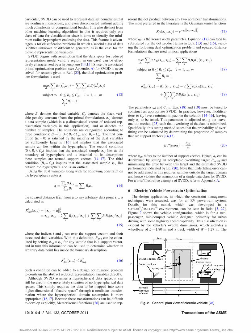
environment, can be seen in Refs. [3, 27].Figure 2 shows the vehicle configuration, which is for a two-passenger, minicompact vehicle designed primarily for urbandriving with some highway speed capability. This classification isevident by the vehicle’s overall dimensions, which includes awheelbase of L¼ 1.80 m and a track width of W¼ 1.27 m. The

Fig. 2 General plan view of electric vehicle [23]



vehicle is powered by a lithium-ion battery energy storage system,which can vary in length, width, and longitudinal location relativeto the front end of the battery compartment such that it lies withinthe dashed region defined by blmax ¼ 1.05 m and widthbwmax¼ 1.20 m. Two electric traction motors drive the rear wheelsthrough a synchronous belt-drive system and are mounted at thepivots on the rear suspension trailing arms to reduce the unsprungmass in the system. A MacPherson strut configuration is used forthe front suspension, and finally, low rolling resistanceP145=70R12 tires are used to minimize the energy consumption.All physically meaningful decision variables (i.e., non-reducedrepresentation variables) for the ATC design problem formulationare listed in Table 1.

6.1 Reduced Representations: POD. Since the ATC designproblem decomposition required the highly discretized motormaps to become decision variables during optimization, reducedrepresentation was necessary. Three POD models were developedto approximate functional data vectors associated with the maxi-mum and minimum motor torque curves and the power loss map

zmax � Up;maxzr;max þ zmax (21)

zmin � Up;minzr;min þ zmin (22)

zpLoss � Up;pLosszr;pLoss þ zpLoss (23)

The functional data vectors zmax and zmin contained qmax¼ qmin¼ 41discretized points each, whereas the functional data vector zpLoss

contained qpLoss¼ 3321 discretized points. The sample functionaldata vectors used to construct the POD representations were gener-ated from an electric traction motor analysis model [3,27] through aLatin hypercube experimental design of m¼ 500 motor maps (seeAppendix B). Because qmax¼ qmin�m, the direct method was usedto develop Up,max and Up,min, whereas the method of snapshots wasused to develop Up,pLoss since qpLoss�m. The CPV was set toCPVgoal¼ 99.99% based in part on the literature [22] as well as pre-vious work [28]. This resulted in reduced representations zr,max,zr,min, and zr,pLoss of dimension pmax¼ 14, pmin¼ 13, andppLoss¼ 89, respectively. Hence, the combined dimensionality of thefunctional data vectors was reduced from Q¼ qmaxþ qmin

þ qpLoss¼ 3403 to Q¼ pmaxþ pminþ ppLoss¼ 116.

6.2 ATC Problem Formulation. The ATC problem formu-lation for the EV powertrain model consists of a two-level hier-archical decomposition. Battery and belt-drive transmissiondesign as well as motor map selection is performed at the top-level subproblem, whereas detailed motor design is performed atthe bottom-level subproblem. The top-level objective is to maxi-mize the gasoline-equivalent fuel economy mpge while minimiz-

ing inconsistencies with the bottom-level subproblem (through p),while the bottom-level objective is to minimize the inconsistencywith the top-level subproblem. Although both subproblems aresubject to decision variable bound constraints, only the top-levelcontains additional constraints based on battery packaging, accel-eration performance, motor feasibility, vehicle range, power avail-ability, and battery capacity.

Applying Eq. (11) directly, the vehicle subproblem P11, exclud-ing decision variable bound constraints, is formulated as

minx11

�mpgeðx11Þ þ vT22t22 þ w22 ðt22 � r22Þk k2

2

subject to

g11;1 ¼ bw;Vðx11Þ � 0 g11;5 ¼ xVðx11Þ � 0

g11;2 ¼ b‘;Vðx11Þ � 0 g11;6 ¼ Rmin � Rðx11Þ � 0

g11;3 ¼ t60ðx11Þ � t60max � 0 g11;7 ¼ PVðx11Þ � 0

g11;4 ¼ sVðx11Þ � 0 g11;8 ¼ Cbðx11Þ �Cbmaxðx11Þ � 0

where

x11 ¼ ½BI ;BW ;BL; xbatt;pr; zTr;comb;x

Tmax; mT

m; JTr ; I

Tym; I

Tzm; y

Tm�

t22 ¼ ½zTcomb;x

Tmax; mT

m; JTr ; I

Tym; I

Tzm; y

Tm�; zT

comb ¼ fðzTr;combÞ

r22 ¼ ½zRcomb;x

Rmax; mR

m; JRr ; I

Rym; I

Rzm; y

Rm�

(24)

where g11,1 and g11,2 are battery width and length packaging con-straints, g11,3 is a performance (0-60 mph acceleration time) con-straint, g11,4 and g11,5 are motor torque and speed feasibilityconstraints, g11,6 is a vehicle range constraint, g11,7 is a poweravailability constraint, and g11,8 is a battery capacity constraint.The vectors zcomb¼ [zmax, zmin, zpLoss] and zr,comb¼ [zr,max, zr,min,zr,pLoss] refer to the combined vector of functional data variablesand the combined vector of reduced representation variables,respectively. Additionally, the vectors t22 and r22 include sixscalar-valued coupling variables: xmax, mm, Jr, Iym, Izm, and ym.Finally, the superscripts T and R denote target and response ver-sions of the same coupling variable, respectively. The motor sub-problem P22, excluding decision variable bound constraints, isformulated in a similar manner as

minx22

�vT22r22 þ w22 ðt22 � r22Þk k2

2

where x22 ¼ ½‘s; rm; nc;Rr�t22 ¼ ½zT

comb;xTmax; mT

m; JTr ; I

Tym; I

Tzm; y

Tm�

r22 ¼ ½zRcomb;x

Rmax; mR

m; JRr ; I

Rym; I

Rzm; y

Rm� ¼ fðx22Þ

(25)

The problem formulation shown in Eqs. (24) and (25) was solvedusing the penalty value-based heuristic and its SVDD-augmentedalternative as constraint management methods for the reduced rep-resentation variables in the P11 subproblem. NOMADm [29], aderivative-free optimization software package based on mesh-adaptive search algorithms, was used as the optimizer. The defaultsettings were modified for the P11 subproblem such that only aLatin hypercube search was performed and 1000 function evalua-tions were permitted. This was necessary to alleviate computationalissues associated with memory availability. However, for the P22

subproblem, the default settings were sufficient. Finally, in theATC coordination strategy, the weight update parameter was set tob¼ 2.75, the initial weight vectors for both subproblems were setto v¼ 0 and w¼ 1, and the tolerance on jjc(K) � c(K�1)jj1 for outerloop convergence was set to 10�2. All computational work wasperformed on a 3 GHz, 4 MB RAM, Intel

VR

CoreTM 2 Duo CPU.

6.3 Constraint Management via Penalty Value-BasedHeuristic. In order to implement the penalty value-based heuris-tic for constraint management, a MATLAB

VR

try-catch conditional

Table 1 Physically meaningful decision variables for ATCdesign problem formulation

Quantity Definition

BI Battery electrode insertion scaleBW Battery cell width scaleBL Number of cell windingsxbatt Battery compartment clearance (m)pr Belt-drive ratioxmax Maximum motor speedmm Motor mass (kg)Jr Rotor moment of inertia (kg-m2)Iym Motor pitch inertia (kg-m2)Izm Motor yaw inertia (kg-m2)ym Motor lateral center of mass location (m)ls Motor stack length (m)rm Rotor radius (m)nc Number of turns per stator coilRr Rotor resistance (X)



statement was written as seen in Fig. 3. This attempts to performthe powertrain simulations and, upon failing, returns infinite val-ues as appropriate for mpge, t60, R, and PV. Note that bw,V, b‘,V,and Cb are not penalized since they are independent of the reducedrepresentation variables, while sV and xV are not included becausethey inherently penalize inaccurate motor maps when the reducedrepresentation variables are outside their model validity region.

Tables 2–4 show the ATC optimization results when imple-menting this constraint management technique. Convergence wasachieved after 12 ATC iterations with a runtime of approximately10.72 hours and resulted in a system solution that was reasonablyconsistent between both subproblems. The only active constraintswere the upper bound on xmax

T , the performance constraint g11,3,and the battery capacity constraint g11,8 in the P11 subproblem;these were limited to xmax

T ¼ 755 rad=s, t60max¼ 10 s, andCbmax¼ 200 Ah, respectively. The optimal values of the PODcoefficients are not listed here as they are too numerous and notphysically meaningful; however, the optimal motor map com-puted by these reduced representation variables is shown in Fig. 4.Finally, the total mass of the vehicle was 1111 kg, with approxi-mately 14.3% (158 kg) of the mass associated with the battery.These design conditions indicated that the EV could achieve a

gasoline-equivalent fuel economy of mpge¼ 184 mpg and a rangeof R¼ 134 miles.

6.4 Constraint Management via SVDD Augmentation. Inorder to implement the SVDD augmentation for constraint man-agement, three kernel-based SVDD models were developed usingEqs. (17)–(19) along with the tuning requirement given in Eq.(20) to approximate the POD model validity regions for zr,max,zr,min, and zr,pLoss. This generated the following additional con-straints for the P11 subproblem in ATC

g11;9 ¼ R2dist;maxðx11Þ � R2

hyp;max � 0 (26)

g11;10 ¼ R2dist;minðx11Þ � R2

hyp;min � 0 (27)

g11;11 ¼ R2dist;pLossðx11Þ � R2

hyp;pLoss � 0 (28)

Figures 5–7 display portions of the optimal SVDD boundaries forthe first two dimensions of the POD model validity regions forzr,max, zr,min, and zr,pLoss. Although the boundaries may appear“loose” (or in the case of the zr,pLoss, nonexistent), it is noted thatthe data set are multidimensional and hence what appears “loose”in one 2D projection may be “tight” in another 2D projection. Thesamples used to construct the SVDD models were identical tothose used for the POD representations but mapped appropriately

Fig. 3 Penalty value-based heuristic: MATLABVR try-catchstatement

Fig. 5 Partial SVDD boundary, max-torque POD model validityregion

Table 2 Optimal decision vector for P11 subproblem, PVBH

BI BW BL xbatt pr xmaxT mm

T JrT Iym

T IzmT ym

T

0.74 1.43 19.75 0.25 3.13 755 40.39 0.28 1.12 1.20 0.39

Table 3 Optimal decision vector for P22 subproblem, PVBH

ls rm nc Rr

0.098 0.123 17.62 0.053

Table 4 Optimal consistency constraint vector=weights, PVBH

Consistency constraint copt vopt wopt

cz,max 0.45 6.37� 108 6.80� 104

cz,min 0.41 5.82� 108 6.80� 104

cz,pLoss 0.73 1.01� 109 6.80� 104

cxmax 0 0 6.80� 104

cmm �0.46 �6.53� 108 6.80� 104

cJr 0 1.51� 106 6.80� 104

cIym 0 5.93� 106 6.80� 104

cIzm �0.02 �3.21� 107 6.80� 104

cym 0 3.67� 106 6.80� 104

Fig. 4 Optimal motor map, PVBH



into POD coefficient-space via the relationships in Eqs. (21)–(23).Also, the slack variable penalty constant was set to Cp¼ 0.5 basedon experience, and a relatively high overfitting target ofPtarget¼ 0.10 [15] was selected for each SVDD model to facilitatea sort of “worst case” comparison to the existing constraint man-agement method. Specifically, since the SVDD samples in thiswork are numerous and derived from relatively well-defined sour-ces (e.g., motor map samples from a model with well-defined lim-its projected into POD coefficient space), setting high overfittingtargets could lead to high occurrences of overconstrained reducedrepresentation variables. This could in turn provide suboptimalresults in terms of accuracy and even efficiency when comparedto the exclusive penalty value-based heuristic; therefore, if theSVDD augmentation could succeed under such unfavorable con-ditions, one could reasonably conclude it would offer greater ben-efits when used more suitably.

The ATC optimization results when implementing the SVDDaugmentation as a constraint management technique for thereduced representation variables are shown in Tables 5–7. Recallfrom Sec. 2 that the penalty value-based heuristic is still includedin this study since the optimizer may periodically violate theSVDD constraints, thus likely leading to model failure whichSVDD alone cannot detect and circumvent. The problem con-

verged after 5 ATC iterations with a runtime of approximately 3.95h and resulted in a system solution that was reasonably consistentbetween both subproblems. The only meaningful active constraintsincluded the upper bound on xmax

T and the battery capacity con-straint g11,8 in the P11 subproblem, which were limited toxmax

T ¼ 755 rad=s and Cbmax¼ 200 Ah, respectively. Althoughthe SVDD constraints g11,9-g11,11 were active as well, they were in-significant from a design perspective and only relevant mathemati-cally. In particular, the activity of the SVDD constraints indicatedthat the optimal reduced representation variables were at theboundary of their respective POD model validity regions. The opti-mal motor map computed by the POD coefficients is shown in Fig.8. Finally, the total mass of the vehicle was 1111 kg, with approxi-mately 14.3% (158 kg) of the mass associated with the battery.With such a design, the EV is predicted to have a gasoline-equivalent fuel economy of mpge¼ 149 mpg, a 0-60 mph accelera-tion time of t60¼ 8.05 s, and a range of R¼ 109 miles.

6.5 Summary of ATC Results. It is clear from the resultsthat the SVDD augmentation improves the efficiency of ATC com-pared with the penalty value-based heuristic. Indeed, the runtimesassociated with the penalty value-based heuristic and the SVDDaugmentation were 10.72 h and 3.95 h, respectively. The improvedefficiency using the SVDD augmentation was due to the explicitconstraints imposed on the POD model validity regions, whichenabled the optimizer spent less time (i.e., fewer function evalua-tions) exploring designs outside the feasible decision space. Never-theless, although the SVDD augmentation reduced thecomputational time during optimization, it still required significantmodeling time offline. Therefore, it is more appropriate to considerthe total computational effort (modeling time plus runtime) whenassessing any efficiency gains via SVDD. The modeling timesrequired to construct the optimal SVDDs for the POD model valid-ity regions of zr,max, zr,min, and zr,pLoss were 0.94 h, 1.13 h, and0.27 h, respectively. Because the total computational effort (6.29h) associated with the SVDD augmentation was less than the run-time associated with the penalty value-based heuristic, it is clearthat the SVDD augmentation was more computationally efficient.

Fig. 6 Partial SVDD boundary, min-torque POD model validityregion

Fig. 7 Partial SVDD boundary, power loss POD model validityregion

Table 5 Optimal decision vector for P11 subproblem, SVDDaugmentation

BI BW BL xbatt pr xmaxT mm

T JrT Iym

T IzmT ym

T

0.74 1.43 19.75 0.25 3.93 755 40.39 0.28 1.12 1.20 0.39

Table 6 Optimal decision vector for P22 subproblem, SVDDaugmentation

ls rm nc Rr

0.096 0.124 17.87 0.065

Table 7 Optimal consistency constraint vector=weights, SVDDaugmentation

Consistency constraint copt vopt wopt

cz,max 0.45 449 57.2cz,min 0.42 416 57.2cz,pLoss 0.29 297 57.2cxmax 0 0 57.2cmm 0 �0.45 57.2cJr 0 0.019 57.2cIym 0 �0.031 57.2cIzm 0 0.035 57.2cym 0 0.025 57.2



To facilitate the comparison of the ATC solutions on the basis ofaccuracy, the corresponding all-in-one (AiO) problem formulationwas solved and its optimal design vector x� ¼ ½BI;BW ;BL;xbatt; pr; ls; rm; nc; Rr� was used to determine the error of each ATCsolution using a normalized Euclidean norm. These errors were0.113 and 0.110 for the design solutions associated with the penaltyvalue-based heuristic and SVDD augmentation, respectively. Thissuggests that the SVDD augmentation enabled only a modestlymore accurate solution than the penalty value-based heuristic.Moreover, since the AiO design solution predicted key performancemetrics (mpge¼ 195 mpg, t60¼ 10 s, and R¼ 100 miles) that weremore consistent with the design solution associated with thepenalty value-based heuristic, one might even question the assess-ment of any accuracy improvement using SVDD augmentation.However, note that the ATC termination condition (jjc(K) �c(K�1)jj1� 10�2), which was affected by the significantly smallerconsistency constraint values for SVDD augmentation, preventedthe optimization strategy from performing an extra outer loop itera-tion that would have likely reduced pr (the main error contributor)in order to achieve better mpge. This would have been done at theexpense of t60 and R, which is consistent with the AiO solution.Hence, it is reasonable to conclude that the SVDD augmentationyielded an accuracy improvement over the penalty value-based heu-ristic, and that this improvement might be more than modest whentaking the details of the optimization strategy into account.

The accuracy improvement with SVDD augmentation can alsobe directly attributed to its constraints, which forced the optimizerto perform more function evaluations in the feasible decisionspace, including the POD model validity regions. Because thisincreased the set of feasible designs, the optimizer had a higherprobability of identifying the optimal design solution instead ofconverging to any feasible (yet suboptimal) design. Conversely,the penalty value-based heuristic enabled the optimizer to performfunction evaluations in a broader decision space, which includedmany infeasible designs. Since this limited the set of feasibledesigns, the optimizer had a higher probability of converging toany feasible (yet suboptimal) design instead of identifying theoptimal design solution. Of course, it is always possible that theSVDD augmentation could truncate a portion of the feasible deci-sion space, where the optimal solution exists and lead to an infe-rior result when compared with the penalty value-based heuristic;however, the probability of this event is ultimately related to thevalue prescribed for Ptarget in the SVDD models.

7 Conclusions

It is evident that the best constraint management method forabstract reduced representation variables in decomposition-baseddesign optimization is the SVDD augmentation. This technique

achieved our main objective of producing better-conditionedoptimization problems with significantly reduced runtimes.While it is expected that SVDD’s computational savings wouldbe observed for any optimization problem (including AiO prob-lems) containing abstract decision variables, the most significantpayoff is for decomposition-based optimization problems sincethese strategies iteratively solve subproblems within their struc-ture. Additionally, the SVDD augmentation can yield moreaccurate design solutions, which is compelling when one con-siders that a “worst case” comparative study was performed bysetting a high overfitting target for the SVDD models. In partic-ular, we can anticipate even more accuracy improvements whenthe overfitting target is set more appropriately. This is of coursea challenge since setting this parameter too conservativelyyields poor boundary descriptions, while setting it too aggres-sively can possibly truncate a design region containing the opti-mal solution. The systematic balance of these tradeoffs isproposed as a topic of future work.

Acknowledgment

This research has been partially supported by the AutomotiveResearch Center, a U.S. Army RDECOM Center of Excellenceheadquartered at the University of Michigan. This support isgratefully acknowledged.

Appendix A

Formally, the objective of SVDD is to solve the following pri-mal optimization problem:

minRhyp;a;ni

R2hyp þ Cp

Xi

ni

subject to zr;i � a 2

2� R2

hyp þ ni; i ¼ 1;…;m

(A1)

where Rhyp denotes the hypersphere radius, ni denotes a hyper-sphere radius slack variable, Cp denotes the slack variable penaltyconstant, zr,i denotes a data sample, a denotes the hyperspherecenter, and m denotes the number of samples. The second term inthe objective function of Eq. (A1) relaxes the optimization prob-lem and permits the inclusion of outliers. To switch to the dualoptimization problem, we must first construct the Lagrangian

LðRhyp; a;Bi; ni;liÞ ¼ R2hyp þ Cp

Xi

ni

�X

i

Bi R2hyp þ ni � zr;i � a

2

2

� �

�X

i

lini (A2)

with non-negative Lagrange multipliers Bi and li. ApplyingKarush-Kuhn-Tucker conditions to Eq. (A2) yields the followingconstraints (along with the dual problem formulation):

Xi

Bi ¼ 1 (A3)

a ¼P

i Bizr;iPi Bi

¼X

iBizr;i (A4)

Cp � Bi � li ¼ 0; i ¼ 1;…;m (A5)

The performance of SVDD is illustrated for the closed-curveshape in Fig. 9 that is bounded by the following functions:

f1ðxÞ ¼ 10 sinðpxÞ=px; x 2 ½�2:93; 2:93� (A6)

f2ðxÞ ¼1

4x4 � 5x2 � 30� �

; x 2 ½�2:93; 2:93� (A7)

Fig. 8 Optimal motor map, SVDD augmentation



To generate an approximation of this boundary, SVDD wasapplied using m¼ 300 data samples and setting Cp¼ 0.5 andPtarget¼ 0.10 appropriately based on experience. Figure 10 showsthe optimal boundary approximation for the closed-curve shape.Although the SVDD approximation is not exact, it is reasonablyaccurate for the constraint management application that isdescribed in this paper. That is, for a single class of known data(i.e., samples) and in the absence of physically meaningful sup-porting information, SVDD can generate an appropriate estimateof a data space boundary.

Appendix B

An error metric known as accuracy and validity algorithm forsimulation (AVASIM) [30] was used to determine both the num-ber of samples as well as the accuracy of the POD representations.This method characterizes the local and global error between orig-inal functional data and their approximations through l1-normsand residual sums. Using these measures, error indices are con-structed such that non-negative values of the combined index indi-cate valid approximations with accuracy levels between 0 and 1,and negative values of the combined error index generally indi-cate invalid approximations. Validity is defined by approxima-tions that lie within some threshold value; therefore, a value of 0indicates that the approximation is at the threshold and valid,whereas a value of 1 indicates that an approximation is completelyaccurate. Recently, this method was extended to two-dimensional

functional data [31], which were necessary for the accuracyassessment of the power loss map in this study. An appropriatenumber of samples for the POD representations was then deter-mined by ensuring that the combined error indices for the motortorque curves and power loss map were positive when averagedacross all current samples and at least three standard deviationsaway from 0 (as set by the threshold value). This conventionwould theoretically ensure that the majority of the POD approxi-mations of the motor maps would be reasonably accurate andvalid. For the current study, this led to m¼ 500 samples whenAVASIM was applied with a 10% tolerance (i.e., threshold value).As a point of further verification, POD approximations for theoptimal motor map produced from the AiO optimization problemequivalent to the ATC optimization problem were measuredthrough AVASIM with the same threshold value and found to beboth reasonably accurate and valid (see Table 8 and Figs. 11and 12).

Fig. 11 Torque curve comparison for AiO optimal motor map

Table 8 AVASIM results for POD-approximated AiO optimalmotor map

Index Max-torque Min-torque Power loss

Ecombined 0.964 0.979 0.809

Fig. 9 Closed-curve shape for SVDD comparison

Fig. 10 SVDD boundary approximation for closed-curve shape

Fig. 12 Power loss map relative error for AiO optimal motormap



References[1] Kim, H. M., 2001, “Target Cascading in Optimal System Design,” Ph.D. Dis-

sertation, University of Michigan, Ann Arbor, MI.[2] Kim, H. M., Michelena, N. M., Papalambros, P. Y., and Jiang, T., 2003, “Target

Cascading in Optimal System Design,” ASME J. Mech. Des., 125(3), pp.474–480.

[3] Alexander, M. J., 2011, “Management of Functional Data Variables inDecomposition-Based Design Optimization,” Ph.D. Dissertation, University ofMichigan, Ann Arbor, MI.

[4] Alexander, M. J., Allison, J. T., and Papalambros, P. Y., 2011, “Reduced Repre-sentations of Vector-Valued Coupling Variables in Decomposition-BasedDesign Optimization,” Struct. Multidiscip. Optim.

[5] Kokkolaras, M., Louca, L. S., Delagrammatikas, D. J., Michelena, N. F., Filipi,Z. S., Papalambros, P. Y., Stein, J. L., and Assanis, D. N., 2004, “Simulation-Based Optimal Design of Heavy Trucks by Model-Based Decomposition: AnExtensive Analytical Target Cascading Case Study,” Int. J. Heavy VehicleSyst., 11(3=4), pp. 402–431.

[6] Wagner, T. C., and Papalambros, P. Y., 1993, “A General Framework forDecomposition Analysis in Optimal Design,” ASME Adv. Des. Autom., 65,pp. 315–325.

[7] Sirovich, L., 1987, “Turbulence and the Dynamics of Coherent Structures. I—Coherent Structures. II—Symmetries and Transformations. III—Dynamics andScaling,” Q. Appl. Math., 43, pp. 561–571, 573–590.

[8] Lucia, D. J., Beran, P. S., and Silva, W. A., 2004, “Reduced Order Modeling:New Approaches for Computational Physics,” Prog. Aerosp. Sci., 40, pp. 51–117.

[9] Alexander, M. J., Allison, J. T., Papalambros, P. Y., and Gorsich, D. J., 2010,“Constraint Management of Reduced Representation Variables inDecomposition-Based Design Optimization,” Proceedings of the ASME Inter-national Design Engineering Technical Conferences and Computers and Infor-mation in Engineering Conference, DETC 2010-28788.

[10] Tarassenko, L., Hayton, P., Cerneaz, N., and Brady, M., 1995, “Novelty Detec-tion for the Identification of Masses in Mammograms,” Proceedings of the 4thInternational Conference on Artificial Neural Networks, pp. 442–447.

[11] Barber, C. B., Dobkin, D. P., and Huhdanpaa, H. T., 1996, “The QuickhullAlgorithm for Convex Hulls,” ACM Trans. Math. Softw., 22(4), pp. 469–483.

[12] Basudhar, A., and Missoum, S., 2010, “An Improved Adaptive SamplingScheme for the Construction of Explicit Boundaries,” Struct. Multidiscip.Optim., 42(4), pp. 517–529.

[13] Basudhar, A., and Missoum, S., 2009, “A Sampling-Based Approach for Proba-bilistic Design With Random Fields,” Comput. Methods Appl. Mech. Eng.,198(47=48), pp. 3647–3655.

[14] Tax, D. M. J., and Duin, R. P. W., 1999, “Data Domain Description Using Sup-

port Vectors,” Proceedings of the European Symposium on Artificial Neural

Networks, pp. 251–256.

[15] Tax, D. M. J., and Duin, R. P. W., 1999, “Support Vector Domain Description,”Pattern Recogn. Lett., 20, pp. 1191–1199.

[16] Malak, R. J., 2008, “Using Parameterized Efficient Sets to Model Alternativesfor Systems Design Decisions,” Ph.D. Dissertation, Georgia Institute of Tech-nology, Atlanta, GA.

[17] Malak, R. J., and Paredis, C. J. J., 2010, “Using Support Vector Machines toFormalize the Valid Input Domain of Predictive Models in Systems DesignProblems,” ASME J. Mech. Des., 132(10), p. 101001.

[18] Karhunen, K., 1946, “Zur spektral theorie stochastischer prozesse,” Ann. Acad.Sci. Fennicae Ser, 34.

[19] Loeve, M., 1945, “Functions aleatorie de second ordre,” C. R. Acad. desSci., p. 220.

[20] Ahmed, N., and Goldstein, M. H., 1975, Orthogonal Transforms for DigitalSignal Processing, Springer, Berlin.

[21] Toal, D. J. J., Bressloff, N. W., and Keane, A. J., 2008, “Geometric FiltrationUsing POD for Aerodynamic Design Optimization,” Proceedings of the 26thAIAA Applied Aerodynamics Conference, AIAA 2008-6584.

[22] Bui-Thanh, T., Damodaran, M., and Wilcox, K., 2004, “Aerodynamic Recon-struction and Inverse Design Using Proper Orthogonal Decomposition,” AIAAJ., 42(8), pp. 1505–1516.

[23] Tosserams, S., Etman, L. F. P., Papalambros, P. Y., and Rooda, J. E., 2006, “AnAugmented-Lagrangian Relaxation for Analytical Target Cascading Using theAlternating Direction Method of Multipliers,” Struct. Multidiscip. Optim., 31,pp. 176–189.

[24] MATLABVR Function Reference, The MathWorks, Inc., Natick, MA.[25] Vapnik, V., 1995, The Nature of Statistical Learning Theory, Springer, New

York.[26] Scholkopf, B., and Smola, J. A., 2002, Learning With Mercer Kernels, MIT,

Cambridge, MA.[27] Allison, J. T., 2008, “Optimal Partitioning and Coordination Decisions in

Decomposition-based Design Optimization,” Ph.D. Dissertation, University ofMichigan, Ann Arbor, MI.

[28] Alexander, M. J., Allison, J. T., and Papalambros, P. Y., 2011,“Decomposition-Based Design Optimization of Electric Vehicle PowertrainsUsing Proper Orthogonal Decomposition,” Int. J. Powertrains, 1(1),pp. 72–92.

[29] Abramson, M., 2007, NOMADm Version 4.5 User’s Guide, Air Force Instituteof Technology, Wright Patterson AFB.

[30] Sendur, P., Stein, J. L., and Peng, H., 2002, “A Model Accuracy and ValidityAlgorithm,” Proceedings of the 2002 ASME International Mechanical Engi-neering Congress and Exposition, IMECE2002-DSC-34284.

[31] Alexander, M. J., and Papalambros, P. Y., 2010, “An Accuracy AssessmentMethod for Two-Dimensional Functional Data in Simulation Models,” Pro-ceedings of the 13th AIAA=ISSMO Multidisciplinary Analysis OptimizationConference, AIAA 2010-9134.



http://dx.doi.org/10.1115/1.1582501

http://dx.doi.org/10.1016/j.paerosci.2003.12.001

http://dx.doi.org/10.1145/235815.235821

http://dx.doi.org/10.1007/s00158-010-0511-0

http://dx.doi.org/10.1007/s00158-010-0511-0

http://dx.doi.org/10.1016/j.cma.2009.07.003

http://dx.doi.org/10.1016/S0167-8655(99)00087-2

http://dx.doi.org/10.1115/1.4002151

http://dx.doi.org/10.2514/1.2159

http://dx.doi.org/10.2514/1.2159

http://dx.doi.org/10.1007/s00158-005-0579-0

http://dx.doi.org/10.1504/IJPT.2011.041910

michael j. alexander constraint management of reduced...

Documents