miao zhao design of digital integrator for rogowski coil
TRANSCRIPT

MIAO ZHAO
DESIGN OF DIGITAL INTEGRATOR FOR ROGOWSKI COIL SEN-SOR
Master of Science Thesis
Examiner: Pro. Timo D. Hämäläinen
Examiner and topic approved by theCouncil of the Faculty of Computingand Electrical Engineering on 4March 2015

2
ABSTRACT
MIAO ZHAO: Design of Digital Integrator for Rogowski Coil SensorTampere University of TechnologyMaster of Science Thesis, 94 pages, 5 Appendix pagesApril 2015Master’s Degree Programme in Information TechnologyMajor: Digital and Computer ElectronicsExaminer: Professor Timo D. Hämäläinen
Keywords: Rogowski coil sensor, digital integrator design, Newton - Cotes Inte-gration, Genetic Algorithm optimization, finite word length effect.
The goal of this thesis is to create a well performed digital Rogowski coil integrator onPC for later implementation on FPGA, and the final filter is applied with fixed pointarithmetic. Integrator’s design and optimization based on the specification provided bythe company. During the implementation, the constraints of the hardware should betaken into account, and the design method needs to be verified by simulations and prac-tical experiments and tests.
There are two design phases to implementing the filter. The first phase is softwareimplementation, the integrator is realized by creating the MATLAB and C models. Theother phase is hardware realization. By software application, the filter could be simu-lated with targeted test benches. After the software application is verified, hardwareimplementation could be carried out if it is necessary. In this thesis, RTL model is de-rived from the C model via translating it with VHDL. Afterward, the integrator is im-plemented on FPGA board for practical field tests.
From the tests, the validity, practicability of the Rogowski integrator have to be verifiedfrom the perspective of both functionality and performance. The software implementa-tion of the integrator is capable of filtering different kinds of the input signals with rea-sonable and acceptable outputs. Meanwhile, in the practical application, the integratorperformed well when dealing with various earth fault cases. All, in brief, this Rogowskiintegrator has to satisfy the standard of the design specification.

3
PREFACE
This thesis was made for the Department of Pervasive Computing, Faculty of Compu-ting and Electrical Engineering, Tampere University of Technology, in cooperation withABB Oy Medium Voltage Products.
I would like to thank my examiner Prof. Timo D. Hämäläinen at Tampere University ofTechnology for help with my thesis plan and the text. I would like to thank mysupervisor Frej Suomi at ABB for the valuable insight during my design of theRogowski coil integrator. Thank Mika Kauppinen and Juha Ekholm for the opportunityto do this thesis at ABB Medium Voltage Products in Vaasa. At last, I’d like to thankmy parents for their unconditional understanding and support for my studying andworking in Finland.
Tampere, 16 March 2015
Miao Zhao

4
TABLE OF CONTENTS
Abstract ...................................................................................................................... 2
Preface ....................................................................................................................... 3
1. Introduction ...................................................................................................... 11
1.1 Background and Motivation ...................................................................... 11
1.2 Requirements and Constraints ................................................................... 11
1.3 Design Platform and Tools ........................................................................ 12
1.4 Organization of Thesis .............................................................................. 13
2. Theoretical Background .................................................................................... 14
2.1 Characteristics of Rogowski Coil Sensor ................................................... 14
2.2 Integrators for Rogowski Coil Sensor ........................................................ 15
2.2.1 Analog and Digital Integrators ...................................................... 15
2.2.2 Digital Filter Design Issues........................................................... 16
2.3 Digital Integration Algorithms................................................................... 24
2.3.1 Direct Design Method Based On the Frequency Response ............ 24
2.3.2 Newton-Cotes Integration Rules ................................................... 25
2.3.3 Pole-Zero Placement .................................................................... 26
2.3.4 Optimization Method ................................................................... 27
3. Digital Integrator Design................................................................................... 31
3.1 Coefficients Calculation ............................................................................ 31
3.1.1 Starting Point Filter Design .......................................................... 32
3.1.2 Coefficients Optimization ............................................................. 41
3.1.3 Design Example ........................................................................... 44
3.2 Structure Realization ................................................................................. 53

5
3.2.1 Available Structures ..................................................................... 53
3.2.2 Finite Word Length Effects Analysis ............................................ 56
4. Filter Implementation ........................................................................................ 61
4.1 Software Implementation .......................................................................... 61
4.1.1 MATLAB Model ......................................................................... 61
4.1.2 C-Language Model ....................................................................... 69
4.1.3 Performance Evaluation ............................................................... 70
4.2 Hardware Implementation ......................................................................... 74
4.2.1 Topology ...................................................................................... 74
5. Testing Results and Analysis ............................................................................ 76
5.1 Functional Verification.............................................................................. 76
5.1.1 Sinusoidal Input ........................................................................... 76
5.1.2 DC Input ...................................................................................... 77
5.1.3 Impulse Input ............................................................................... 78
5.1.4 Noise Input ................................................................................... 79
5.1.5 Complex Input.............................................................................. 80
5.2 Performance Verification .......................................................................... 80
5.2.1 Solid Earth-Fault .......................................................................... 81
5.2.2 Low-ohmic Earth-Fault ................................................................ 82
5.2.3 High-ohmic Earth-Fault ................................................................ 82
5.2.4 Intermittent Earth-Fault ................................................................ 84
5.3 Summary of the Tests ................................................................................ 84
6. Conclusions ...................................................................................................... 85
6.1 Discussion ................................................................................................. 85
6.2 Challenge .................................................................................................. 86

6
References ................................................................................................................ 87

7
LIST OF FIGURES
Rogowski integrator workflow ....................................................... 12
Rogowski Coil’s structure [10] ...................................................... 14
Block diagrams of FIR and IIR filters ............................................ 16
Direct and Transposed Direct Form I Structures ........................... 21
Direct and Transposed Direct Form II Structures .......................... 22
Cascaded second order filter with Direct and Transposed DirectForm I structures ........................................................................... 23
Cascaded second order filter with Direct and Transposed DirectForm II structures ......................................................................... 23
A simple Genetic Algorithm Cycle [39] ......................................... 27
Simple Genetic Algorithm Cycle .................................................... 31
Frequency response of the resulted filter ....................................... 33
Magnitude responses of three filters .............................................. 34
Phase responses of three filters ..................................................... 34
Frequency response of trapezoidal integrator after adding a notch 35
Frequency response of directly designed filter ............................... 36
Magnitude and Phase responses of directly designed filter andcandidate 1 filter ........................................................................... 37
Pole- zero position of the original trapezoidal integrator .............. 38
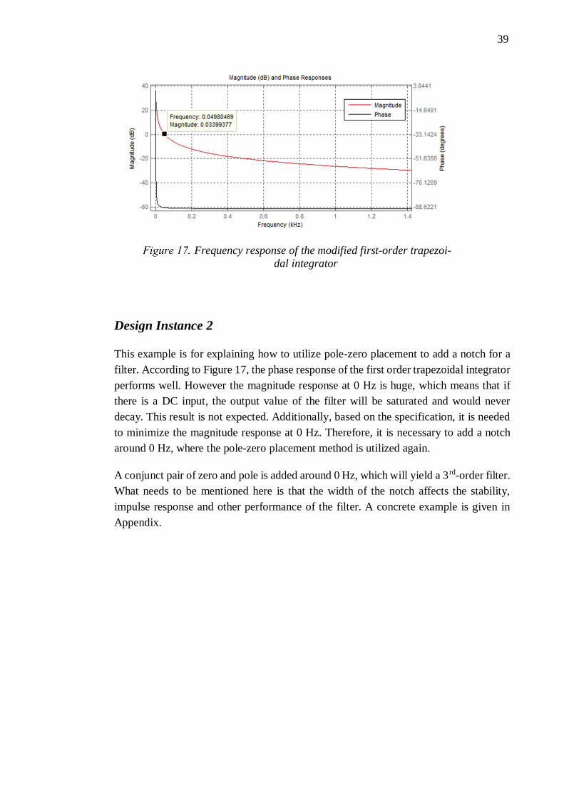
Frequency response of the modified first-order trapezoidal integrator ...................................................................................................... 39
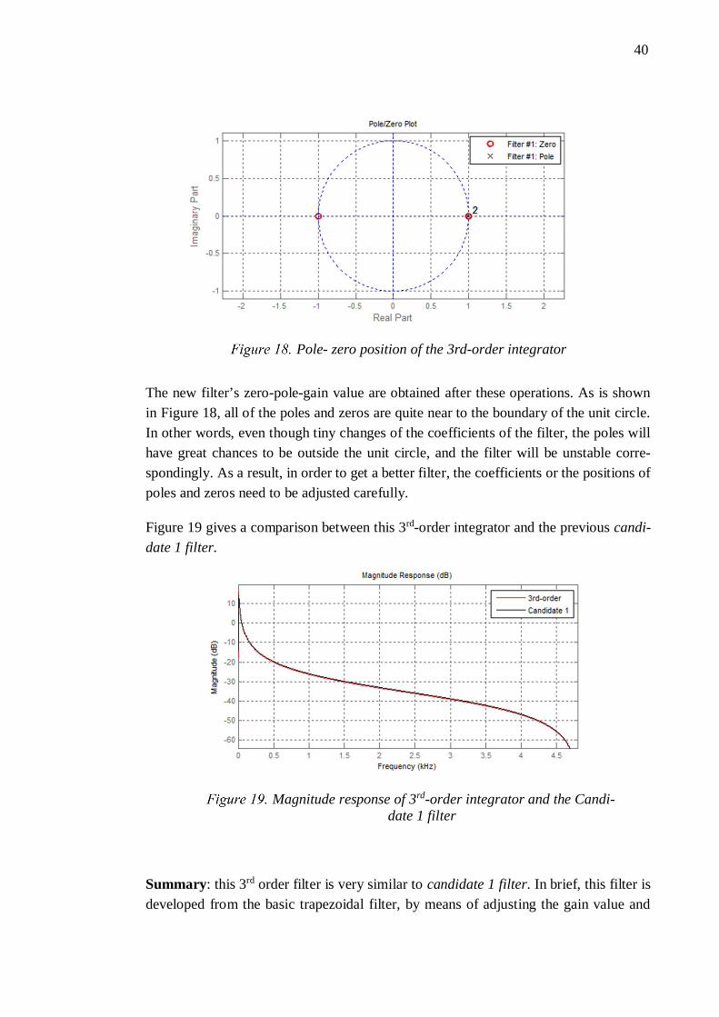
Pole- zero position of the 3rd-order integrator .............................. 40
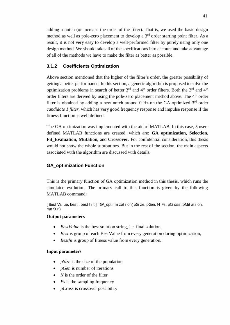
Magnitude response of 3rd-order integrator and the Candidate 1 filter ...................................................................................................... 40
Variation in fitness values through generations with pSize numbers ofa) 20, b) 30 and c) 40 .................................................................... 47

8
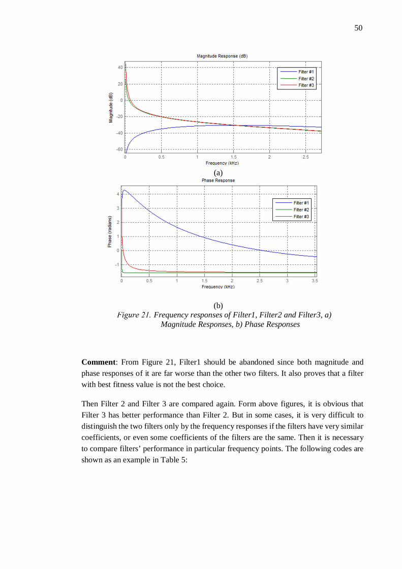
Frequency responses of Filter1, Filter2 and Filter3, a) MagnitudeResponses, b) Phase Responses ..................................................... 50
Impulse and step responses of Filter2 and Filter3 .......................... 52
Direct Form I of the 4th order IIR filter .......................................... 53
Direct Form II of the 4th order IIR filter ........................................ 54
Transposed Direct Form I of the 4th order IIR filter ....................... 54
Transposed Direct Form II of 4th order IIR filter ........................... 55
Cascaded second order filter with Direct Form II .......................... 56
Cascaded second order filter with Direct Form II transposed ........ 56
Pole-zero deviations ...................................................................... 58
Round-off Noise Power Spectrum .................................................. 59
Filtering Functionality Simulation ................................................. 60
The 4th-order filter Cascade Form structure .................................. 61
Filtering results of noise inputs with different amplitudes .............. 64
Filtering results of noise inputs (0.005xIn) with different datatypes .............................................................................................. 65
Filtering results of noise inputs (60xIn) with different data types ... 66
Filtering results of noise inputs (0.5xIn) with different data types .. 66
Filtering results of sinusoidal input (0.005xIn) .............................. 67
Output error comparisons of different data types ........................... 68
Output error comparison of different data types ............................ 68
Block diagram of filter functioning ................................................ 71
Filtering results of test case 1 ........................................................ 71
Output results after one operation on FPGA .................................. 72
Output signals after integration and the error between two signals 72

9
Output signals after integration ..................................................... 73
Filter topology of one section ........................................................ 75
Simulation results with sinusoidal input ......................................... 76
Simulation results with DC input ................................................... 77
Simulation results with impulse input............................................. 78
Simulation results with derivative of impulse input ........................ 78
Simulation results with random noise input ................................... 79
Simulation results with complex input ............................................ 80
Simulation results with solid earth-fault ........................................ 81
Simulation results with low-ohmic earth-fault ................................ 82
Simulation results with high-ohmic earth-fault .............................. 83
Simulation results with intermittent earth-fault .............................. 84

10
LIST OF SYMBOLS AND ABBREVIATIONS
CT Current TransformerAC Analog CurrentPC Personal Computer.FPGA Field-Programmable Gate Array.BIBO Bounded-Input Bounded-Output.ADC Analog -to-Digital Converter.VHDL Verilog Hardware Description Language.LTI Linear Time Invariant.MSB Most Significant BitLSB Least Significant BitGA Genetic Algorithm.RMS Root Mean SquareRTL Register Transfer Level
i Measured current from Rogowski sensorVout Output signal form Rogowski sensorMR Mutual inductanceh(k) Impulse response sequenceZ Complex variablea Denominator of filter coefficientsb Numerator of filter coefficientsN Filter’s order

11
1. INTRODUCTION
1.1 Background and Motivation
In electrical engineering, including power system, current transformers (CTs) have beentraditionally used for protection and measurement applications for the main reason oftheir ability to produce the high power output. However, the emergence of microproces-sor based equipment made high power output unnecessary and introduced other meas-urements techniques. One such measuring device that equips many advantages over CTsis the Rogowski coil transducers [1].
Rogowski coils are commonly incorporated in measuring and protection systemsthroughout the industry and in research. Its feature of “air-cored” offers an advantageover iron-cored measuring devices [2]. Thanks to the benefits of Rogowski coils, suchas high accuracy, excellent linearity, wide dynamic range, wide band and no magneticsaturation, they can replace CTs and be used for protection, metering and controlpurpose in the general electric current measurement field [1], [3], [4], [5], [6], [7]. Theadvantages of Rogowski coil sensor over the traditional current transducers will makeit be more extensively used in the future.
Based on the principle of Faraday’s law of electromagnetic induction, Rogowski coilproduces a voltage output signal which is proportional to the derivative of the currentsignal. An integrator is required to restore the measured AC waveform from the voltagesignal induced in the Rogowski coil sensor [1]. With a well-designed integrator, theRogowski coil can achieve excellent performance such as higher accuracy and betterlinearity than conventional CTs [6]. Thus, an integrator with high performance is thekey to guaranteeing the high measuring accuracy of Rogowski coil sensor [3].
This thesis’ goal is to design a well performed digital Rogowski coil integrator on PCfor later implementation on FPGA. The idea is to find a proper method to design anintegrator with respect to all the specifications and requirements need to be concerned,and improve the performance of the filter as much as possible. Additionally, the con-straints of the hardware should be taken into account, and the design method needs tobe verified by simulations and practical experiments and tests.
1.2 Requirements and Constraints
This thesis was made by request of ABB Oy, Medium Voltage Products in Vaasa. Themain requirements and specifications are listed as below:

12
1. The target frequency range of the integrator is from 10 to 1250 Hz. The integratorwill work in electric power grid with frequency of 50 Hz. Thus, the primary focusshould be paid to the frequency around 50 Hz.
2. For the frequency response, the magnitude response should follow the equationMagnitude = 50 / Frequency as close as possible. The phase response should be -90degree as close as possible.
3. The group delay should be as flat as possible and as small as possible. Additionally,it is better that from 50Hz, the group delay is positive and as close to zero as possi-ble. The max group delay should be no more than two samples when the samplingfrequency is 9600Hz.
4. The filter needs to be implemented with fixed point arithmetic.
5. The step response should decay to zero as near as possible.
6. The filter should be BIBO stable.
7. Measurement and ADC quantization noise should not accumulate to disturbinglylarge DC levels in the integrator.
8. The structure and bit widths of filter implemented on FPGA should be designed tonot suffer too many rounding errors.
1.3 Design Platform and Tools
In this thesis, the optimized integrator is finally implemented on the hardware platform,which is an FPGA applied in a protection relay. Figure 1 briefly shows the generalworkflow, where that Rogowski integrator works.
We developed the integrator in a software approach. To guarantee the computability ofthe filter structure, and as well to verify the accuracy of this structure are of substantialimportance in the design [9]. Thus, before the filter algorithm is finally implemented onthe FPGA board, the digital filter is designed and simulated on PC with the aid ofMATLAB and Visual Studio. All of the early designs and optimizations on the digitalintegrator are done with MATLAB. After that, Visual Studio is used to create a filter
Rogowski integrator workflow

13
model in C language. The C model is utilized for making the VHDL, where the ad-vantage is that C is easier for a VHDL designer to understand that MATLAB code.
1.4 Organization of Thesis
In the subsequent part of this thesis, Chapter 2 introduces the theoretical backgroundrelated to the thesis work. In Chapter 3, specific integrator design algorithms are real-ized, tested and corresponding comparisons are conducted through simulation with theusing of MATLAB. The best design method for the following actual design work ischosen in the end. After deciding the design method of the filter, a detailed explanationof the process of practical design work is introduced in chapter 4. This section containsthe distinct approaches to filter’s software and hardware implementations. Chapter 5provides the testing results of the filter, the analysis of filter’s performance is madeafterward. Chapter 7 consists of the conclusion of the thesis work and possible furtherwork that could be done after this thesis work.
14
2. THEORETICAL BACKGROUND
2.1 Characteristics of Rogowski Coil Sensor
A Rogowski Coil is an air-cored coil, in which the windings are twined evenly on a non-magnetic skeleton. The Rogowski coil has galvanic isolation [45] with the measuredcircuit, which is convenient for isolated measurements of high voltage circuits. Thus, itcan be utilized as sensing element, such as electronic current transformer. The detailedoperation theory of Rogowski coil can be found by referring [9].
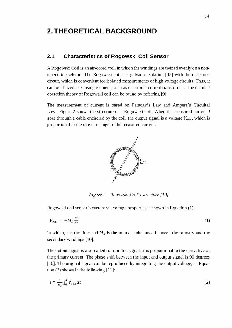
The measurement of current is based on Faraday’s Law and Ampere’s CircuitalLaw. Figure 2 shows the structure of a Rogowski coil. When the measured current Igoes through a cable encircled by the coil, the output signal is a voltage , which isproportional to the rate of change of the measured current.
Rogowski coil sensor’s current vs. voltage properties is shown in Equation (1):
= − (1)
In which, t is the time and is the mutual inductance between the primary and thesecondary windings [10].
The output signal is a so-called transmitted signal, it is proportional to the derivative ofthe primary current. The phase shift between the input and output signal is 90 degrees[10]. The original signal can be reproduced by integrating the output voltage, as Equa-tion (2) shows in the following [11]:
= ∫ (2)
Rogowski Coil’s structure [10]

15
Due to the absence of iron in a Rogowski coil sensor, no magnetic saturation occurs. Asa result, the output is linear over the whole current range up to the highest current. How-ever, in practical the cabling and connectors will restrict the dynamic range.
Intermittent Earth Fault
An imperative reflection of the integrator’s performance is the intermittent earth fault.Intermittent earth fault is a particular type of failure that is encountered mainly in com-pensated grid with underground cables. According to [12], intermittent earth fault “ischaracterized by repetitious of short duration self-extinguishing faults. This kind offailure tends to be difficult for conventional directional earth fault protection relays todetect due to highly irregular wave shape of residual current. Whereas residual over-voltage relays used typically as a substation backup protection have better chances forfault detection because of more steady behavior of residual voltage.” Due to this fact,intermittent earth fault can often cause non-selective tripping of the substation backupprotection and eventually an outage with substantial cost. ” That is why in thesis, aparticular integrator’s performance test for the intermittent earth fault is made. It is nec-essary to guarantee that the integrator functions well under intermittent earth fault.
2.2 Integrators for Rogowski Coil Sensor
2.2.1 Analog and Digital Integrators
Analog and digital methods can implement the integration part of the Rogowski coil.Analog integrators are usually composed of inertial elements such as amplifier, resistors,and capacitors. Currently, analog integrators are generally at the end of Rogowski coilsto transform input current’s amplitude and phase. However, analog devices are not tem-perature and aging stable, which could cause problems, such as leakage, loss of capacityand zero-drift in the analog devices. In addition, it is relatively inflexible to design thefeedback and compensation of an analog integrator [13]. All of these factors existing inanalog devices are potential to result in integration errors.
Digital integrator, however, possesses the outstanding features which overcome the in-herent weak points of analog one. It is based on the sampling algorithm, which samplesthe signal directly and then restores the original signal by numerical integration meth-ods. Furthermore, the disadvantages of classical analog integrator, such as thermal andtime stability, could be entirely avoided [14].
Digital integrator, featuring higher accuracy and stability, good phase response perfor-mance as well as flexible structures, are used widely now in Rogowski coil sensors [15].There are several methods, such as using Data acquisition card and PC to implementdigital integrators, the most common method is using ADC and DSP to realize the digitalintegrator [14].
16
Therefore, in this paper, a digital integrator of the Rogowski coil was designed,using several integration algorithms.
2.2.2 Digital Filter Design Issues
The design of digital integrators is essentially the design of digital filters. According to[16], “A digital filter is a system that implements a mathematical algorithm in hardwareand/or software, in order to achieve the filtering goal in a particular region of a signalspectrum.”
Types and Representations
Digital filters can be categorized into several groups depending on the criteria used forclassification. The two main types of digital filters are finite impulse response (FIR) andinfinite impulse response (IIR) filters. Both of the filters can be represented by the im-pulse response sequence, which is often denoted as ℎ( )( = 0, 1, … ) [16]. Since thedigital filters we are going to design are linear and time-invariant (LTI), the generalforms of FIR filter and IIR filter can be expressed as:
( ) = ∑ ℎ( ) ( − ) (3)
( ) = ∑ ℎ( ) ( − ) (4)
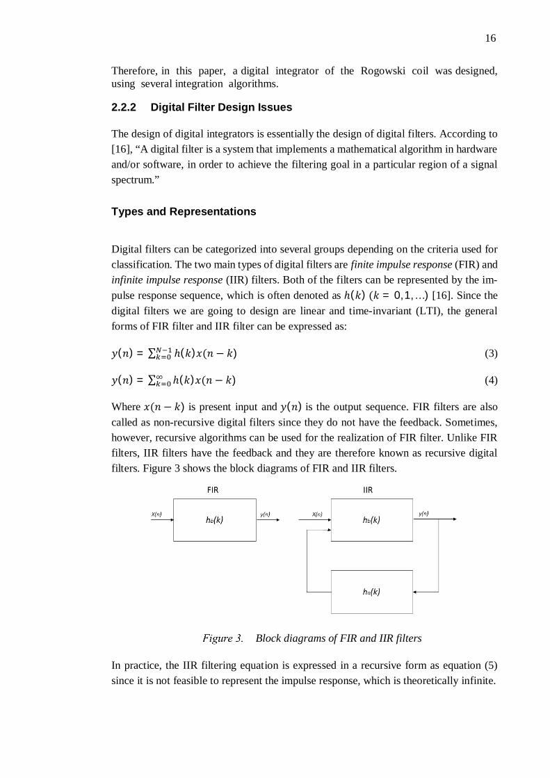
Where ( − ) is present input and ( ) is the output sequence. FIR filters are alsocalled as non-recursive digital filters since they do not have the feedback. Sometimes,however, recursive algorithms can be used for the realization of FIR filter. Unlike FIRfilters, IIR filters have the feedback and they are therefore known as recursive digitalfilters. Figure 3 shows the block diagrams of FIR and IIR filters.
In practice, the IIR filtering equation is expressed in a recursive form as equation (5)since it is not feasible to represent the impulse response, which is theoretically infinite.
Block diagrams of FIR and IIR filters

17
( ) = ∑ ℎ( ) ( − ) = ∑ ( − ) −∑ ( − ) (5)
Where and are the coefficients of the filter. Equation (3) and (4) below are alsorespectively called as difference equations for FIR and IIR filters. For LTI as well ascausal filters, FIR and IIR filters can be expressed as transfer functions in the Z-domain,then the forms could be like the following:
( ) = ∑ ℎ( ) (6)
( ) = ∑ /( 1 + ∑ ) (7)
Where the filter order equals to the greater one of M or N (in FIR filter, the order equalsto N). Transfer functions are of huge importance in evaluating the frequency responsefor the filters.
FIR and IIR can also be differentiated by visualizing the place of the poles. For FIRFilter, all of the poles of the filters locate at the origin, and, as a result, the shape of thefrequency responses are determined only from the locations of the zeroes. On the otherhand, IIR filters have the poles to move inside the unit circle, permitting them to con-tribute more heavily to the shape of the frequency responses.
For FIR filters, they often have linear phase responses, and they are always stable. Whencomparing with the IIR filters, it frequently needs higher filter order than FIR filters toachieve the same response for fixed specifications [16]. As a price, for IIR filters, theyalways have non-linear phase responses and have big potentials to be unstable.
Digital Filter Design Issues
Selection of Filter Type
It is always a trade-off between the choices of IIR and FIR filters. However, the decisionis mostly dependent on the specific design conditions. It is much easier to choose FIRfilter when there is a need for linear phase, and there is no strict requirement on the filterorder. However, when considering the filter order or when particular phase response isneeded, it is better to choose IIR filter. Even though, there is a big risk to get unstablefilter during the design. In many applications, the linearity of the phase response is notas important as the computational efficiency [8]. However, in this thesis, specific phaseresponse is required, and with the resource consumption of hardware taken into account[18], which makes IIR filter a better choice.
General Design Steps
Following are the design steps for an IIR filter in this thesis:
18
1. Filter Specification. Filter specification determines the characteristics of the de-sired filter and indicates the requirements we should meet during the design pro-cess. The objective of designing a digital filter is to develop a causal transferfunction ( ) which can satisfy the filter specifications.
2. Coefficients Calculation. When the specification is made, an essential step is todecide the transfer function, which could realize the filter frequency responsespecifications as well as possible. In other words, it means to find out the optimalfilter coefficients. The filter’s order needs to be estimated after the selection ofthe digital filter type. There are several approaches to developing a filter, theparticular method is based on the transfer function and the filter specifications.Additionally, it is necessary to guarantee the filter to be stable when an IIR filteris desired.
3. Structure Realization. For IIR and FIR filters, there are different kinds of struc-tures. IIR filters often use direct, cascade and parallel forms, for FIR filters, di-rect form is widely used. When considering the finite word length problems,cascade and parallel structures are better choices than direct form in IIR filterdesign, as cascade and parallel structures have fewer coefficient sensitivityproblems than direct forms, especially when they are with high filter order. Inmany applications, a higher order IIR filter is implemented either in apresentation of cascade of second-order sections or in the form of a parallel con-nection of second-order sections. Poles are more sensitive to the quantized coef-ficients and other finite word length effects [8].
4. Implementation. The practical filter application is either done in software orhardware, but neither can provide infinite precision for the coefficients as wellas the signal variables. It turns out that direct realization of a digital filter maynot satisfy the designer’s expectation for the performance due to the finite pre-cision arithmetic [9]. Thus, it is necessary to develop new suitable filter struc-tures when converted from transfer function, and to avoid significant finite word-length effects.
Fixed Point Consideration
In digital filters, the arithmetic operations can be coarsely divided into three broad cat-egories: floating-point, fixed-point, and block floating point representations [18]. Weassume floating-point arithmetic of the calculation and approximation steps during thedesign process. Then fixed point arithmetic is employed by replacing the floating pointarithmetic. It is evident that finite word length effects will degrade the filter’sperformance, and the extent of the effects have to be confirmed before the IIR filter is
19
finally implemented. In addition, it is necessary to find a remedy if the degradation isnot acceptable [16].
In the practical filter implementation, it is often necessary to represent the coefficientsby specific number of bits. The number is represented in the way that a binary point isused to separate the integer part from the fractional part [8]. In addition, a sign bit isplaced in the leading position for the signed fixed point number. The fixed point formatvaries depending on the way negative number are represented. In this case, the fixedpoint negative numbers are represented in two’s complement representation. Forexample, a positive number has the sign bit 0 while a negative number has the sign bit1 [20]. In general, the decimal equivalent of a binary number consisting of B1 integerbits and B2 fractional bits, which could be represented as following form [21]:
∑ 2 (8)
From above we get:
… ∆ … (9)
Where each bit is either a 0 or a 1, the leftmost bit is called the most signifi-cant bit (MSB), and the rightmost bit, is called the least significant bit (LSB). ∆denotes the binary point or radix point, which is fixed.
Radix point of a number is used to separate its integer and fractional numeric fields [18].For description convenience, a fixed point number is represented in a form of s B.B2 inthis thesis, where B is the sum of B1 and B2. In other words, B is the total bit width ofthe number, and B2 is the bit width of the fractional part.
The basic arithmetic operations in the implementation of digital filtering algorithms areaddition (subtraction) and multiplication. It should be carefully treated that the arithme-tic of addition and multiplication of two fixed-point binary numbers may result in morebits than those in the two numbers [22]. As a consequence, when the result is storedback in the memory, the result must either be truncated or rounded to fit the memoryword-length. That is one of the word-length effects caused by the finite word length.
The use of finite precision arithmetic leads to three types of finite word-length effects[16].
1. Quantization. The quantization includes input/output quantization and the coef-ficient quantization. We mainly focus on the coefficient quantization in this the-sis. Quantization of the filter coefficients is likely to disturb the locations of thefilter’ poles and zeroes. Then, the corresponding filter response is different fromthe ideal filter response. This deterministic frequency response error is referredto as coefficient quantization error.

20
2. Arithmetic round off errors. Quantization makes it necessary to quantize filtercalculations by rounding or truncation. Round off noise is like low-level noisein the filter output, which comes from rounding or truncating calculations duringthe filtering process.
3. Overflow. With fixed point arithmetic, it is possible for filter calculations tooverflow. The overflow occurs when the result of an addition exceeds permissi-ble word-length.
Structure Realization
Structure realization is based on the known transfer function. The structural representa-tion plays a crucial role in filter implementations, for it provides the relations betweenintermediate variables with the input and the output [8].
For one filter or one transfer function, several equivalent structures are available. How-ever, in practice, when fixed point arithmetic is employed, a particular realization be-haves differently from its other equivalent realizations. Hence, under a fixed point arith-metic, it is necessary to choose a structure which has good quantization propertiescarefully. Here in our case, we only consider the realization problem of IIR filters. Weoutline several common forms that are used in the realization of IIR filters.
Direct Form I Structures
As Figure 4 shows, Direct Form I structure on the left can be regarded as an all-zerofilter section followed in the series by an all-pole filter section. In general, it is alwayspossible to implement a Nth-order filter using only N delay elements (Here we assumeM equals to N). Direct Form I structure needs twice as many delays as are necessary.

21
The right side of the figure shows transposed Direct Form I structure. The differencebetween direct and direct transpose realizations is not significant. Both structures havethe same multiplication coefficients. The position of delays determines the main differ-ence. Similar to direct realization structure, the direct transpose realization structure uses2N delays, (2N+1) multiplications and 2N additions.
One advantage of the direct form I implementation is that it cannot overflow internallyin two's complement fixed-point arithmetic while most IIR filter implementations donot have this property [23]. The disadvantages of this realization includes the greatestsensitivity to the accuracy of coefficients, and the biggest complexity due to implemen-tation.
Direct Form II Structures
Direct and Transposed Direct Form I Structures

22
The direct form II structure is shown on the left side of figure 5[15]. It can be regardedas an all-pole filter section followed by an all-zero filter section. It is canonical withrespect to delays, since the delay elements associated with the all-pole, and all-zero sec-tions are shared with each other. As a result, direct form II realization structure has re-duced number of delays to the minimum, that is, N delays. That is the main advantageover direct form I realization structures.
On the right side of figure 5 is the transposed direct form II structure It uses N delayelements, (2N+1) multiplications and only (N +1) additions, while direct form II needs(N +1) additions.
Unlike direct form I structure, overflow can occur at the delays in direct form II struc-ture with fixed-point arithmetic. In general, all direct-form structures are very sensitiveto round-off errors in the coefficients, especially for filter with high orders. For thisreason, series low-order sections are applied in filter realization to get lower quantiza-tion sensitivity [23].
Cascaded Second-Order
Direct and Transposed Direct Form II Structures

23
As indicated before, under fixed point arithmetic, equivalent structures have differentperformance. Especially when the filter order is high, direct realization of the filter isvery sensitive to finite word-length effects and should be avoided in these cases [16]. Inpractice, the transfer function is broken down into smaller sections, typically secondand/or first order blocks, which are connected in cascade. For a cascaded second orderfilter, there are two 2nd order filters connected in the cascaded form. Figure 6 and Figure7 describe the differences of these two structures.
Cascaded second order filter with Direct and Transposed Di-rect Form I structures
Cascaded second order filter with Direct and Transposed Di-rect Form II structures
24
2.3 Digital Integration Algorithms
This chapter presents several known integrator design practices with general theories.The specific design for a starting point filter will be explained later with details in chap-ter 3.
2.3.1 Direct Design Method Based On the Frequency Response
By analyzing the design specification, there is an explicit requirement for magnitudeand phase response in the particular frequency range of interest. With the help ofMATLAB Signal Processing Toolbox, we could use the function “invfreqz” to generatecorresponding filter coefficients. This function finds a discrete-time transfer functionthat corresponds to a given complex frequency response. From a laboratory analysisstandpoint, “invfreqz” can be used to convert magnitude and phase data into transferfunctions [24, 25]. This function performs like [26]:
[b,a] = invfreqz(h,w,n,m,wt,iter,tol,'trace')
Where the parameters are explained in the following:
· h is the vector that stores the complex frequency response· w is the vector specifying the frequency points· m is the desired order of the numerator· n is the desired order of the denominator· wt is a weighting factors vector of the same length as w· iter is the iteration bounds· tol is the convergence parameter
The function returns the real numerator and denominator coefficients in vec-tors b and a of the transfer function:
( ) = ∑ /( 1 + ∑ ) (10)
Based on the frequency response specification, it is easy to specify the input parameters.It is a very fast way to design a filter. However, the resulted filter performance needs tobe tested since specifying comprehensive frequency points for the filter is difficult tosome extinct, and it could not describe the frequency response in an exact way withgood precision. As a result, the filter we obtained with have deviations from the speci-fications. It is necessary to specify the input parameter carefully during the design, andseveral iterations may do help for getting better coefficients.

25
2.3.2 Newton-Cotes Integration Rules
The transfer function of digital IIR integrators could be derived by the simple applica-tion of z-transform to the difference equations defined by the various numerical integra-tion rules [27, 28]. There are several methods to implement the basic integrators whichare based on the Newton-Cotes integration rules, such as Al-Alaoui’s first-, second- andthird-order integrators and [27, 30], Ngo’s third-order integrator [31]. Newton-cotes in-terpolation formula is a technique that calculates a definite integral/curve by replacingthat curve by a more integrable and simpler curve [32].
In numerical analysis, the Newton-Cotes integration rules are carried out by evaluatingthe integrand at equally spaced points [47]. A related good starting point filter is neces-sary to guarantee the convergence to the optimal solution. A few of the classicalintegrators using newton-cotes rules are worth mentioning, like Trapezoidal Integrator[27], Simpson Integrator [33], Rectangular Integrator, which are among the mostpopular methods for approximating the evaluation of the definite integrals [18]. In thissection, these three integration rules are introduced.
Trapezoidal algorithm
The numerical integration rule of Trapezoidal algorithm [27] could be represented asthe following function:
∫ ( ) ≈ [ ( ) + ( + )]; ℎ = ( − ); (11)
Where, ( ) is the function that needs to be integrated between the interval c to d, andc is smaller or equal to d. The transfer function of the trapezoidal integrator to Z domainis given by:
= (12)
Where T is constant, that is obtained from the transformation. Based on the transferfunction, the coefficients of the integrator are directly obtained in (13). However, thederived filter is not stable, this issue will be discussed later.
Numerator coefficients: b0 = 1, b1 = 1;
Denominator coefficients: a0 = 2, a1 = -2. (13)
Simpson algorithm
The Simpson algorithm [27, 33, 34] could be represented in the following formation:

26
∫ ( ) ≈ ( ) + 4 + ( ) ; ℎ = ( − ); (14)
The transfer function of the Simpson 1/3 integrator is given by:
= (15)
This filter is a third order filter. The coefficients are listed as following:
Numerator coefficients: b0 = 1, b1 = 4, b2 = 1;
Denominator coefficients: a0 = 3, a1 = 0, a2 = -3. (16)
Except for the Simpson 1/3 rule, there is another Simpson 3/8 rule which could yield a4th order filter, which we will not discuss in our case.
Rectangular Algorithm
The Rectangular algorithm [27, 35, 36] could be represented as following:
∫ ( ) ≈ h ∗ f(c); ℎ = ( − ); (17)
The transfer function of the Simpson integrator is given by:
= (18)
This filter is a third order filter. The coefficients are listed as following:
Numerator coefficients: b0 = 0, b1 = 1;
Denominator coefficients: a0 = 1, a1=-1. (19)
2.3.3 Pole-Zero Placement
In general, the frequency response of an ideal digital integrator [32, 37] is given by:
( ) = (20)
Where = √−1 and is the angular frequency in radians.
The filter can be directly derived since the transfer function of this filter is known. Thenby analyzing the specification, new desired filter with higher order is designed by addingextra zeroes and poles to the primary filter. This approach is also known as the pole-zero placement method. When a zero is placed at a given point on the z-plane, the fre-quency response will be zero at the corresponding point. On the other hand, a pole
27
produces a peak at the relevant frequency point. In order to make the filter stable, all ofthe poles need to be inside the unit circle.
2.3.4 Optimization Method
Since the design of digital filters involves multiple design specifications, which are oftenconflicting, generally there is no easy way to an optimal design. Optimization basedmethods are presented to design digital filters that would satisfy the prescribed specifi-cation. However, optimization methods often require more computation work than basicdesign methods and are not so time efficient.
After generating the starting point filter, global optimization method is employed. Ge-netic Algorithm (GA) [38] is a good method to improve on a good but not perfect filter.
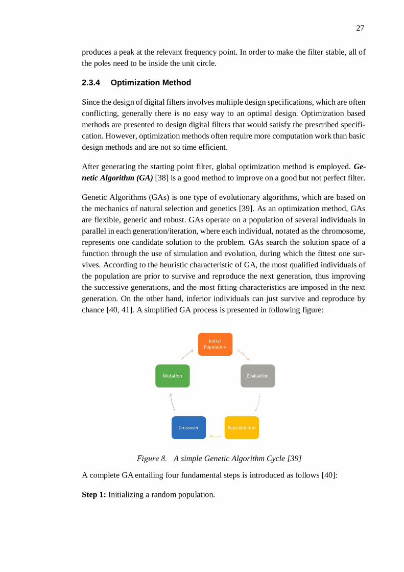
Genetic Algorithms (GAs) is one type of evolutionary algorithms, which are based onthe mechanics of natural selection and genetics [39]. As an optimization method, GAsare flexible, generic and robust. GAs operate on a population of several individuals inparallel in each generation/iteration, where each individual, notated as the chromosome,represents one candidate solution to the problem. GAs search the solution space of afunction through the use of simulation and evolution, during which the fittest one sur-vives. According to the heuristic characteristic of GA, the most qualified individuals ofthe population are prior to survive and reproduce the next generation, thus improvingthe successive generations, and the most fitting characteristics are imposed in the nextgeneration. On the other hand, inferior individuals can just survive and reproduce bychance [40, 41]. A simplified GA process is presented in following figure:
A complete GA entailing four fundamental steps is introduced as follows [40]:
Step 1: Initializing a random population.
A simple Genetic Algorithm Cycle [39]

28
Step 2: Evaluating the fitness of the chromosomes by precisely defined criteria, whichis based on the design requirements for searching the best matching solutions.
Step 3: If the chromosome with best fitness value satisfies the requirements sufficiently,producing that chromosome as the expected solution and stop. Otherwise, continue toStep 4.
Step 4: Applying crossover and mutation among the chromosomes to generate morechromosomes, and then restart at Step 2.
Then the derived algorithm is summarized with specific notations in the following [40]:
1 Supply a population P0 of N individuals and correspondingfitness value for each individual in one generation.
2 Iteration from 1 to i
3 Choose individuals from selection function ( − 1) forreproduction.
4 New generation is got from reproduction function
5 Evaluate ( ) by evaluation function
6 Jump to next generation i=i+1
7 Repeat Step (3) until termination
8 Print out best solution found
Six fundamental issues are used in a GA algorithm: chromosome representation,selection function, genetic operators, initial population, termination criteria, andthe fitness function. These issues will be discussed separately later in this section [41].
Chromosome Representation
In a Genetic Algorithm, chromosome representation is used for describing the individ-uals who will be manipulated by other functions. According to [40], “The chromosomerepresentation is crucial for a GA since the representation scheme determines how theproblem is prototyped in GA and affects the determination of other genetic operators.Each chromosome consists of a sequence of genes from a particular alphabet. Analphabet could be made of binary digits, floating point numbers, integers, symbols, ma-trices, etc.”
29
Selection Function
The purpose of individual selection is to create new successive generations. Selectionplays a crucial role in a GA. A probabilistic selection is performed based on the individ-ual’s fitness value so that the better individuals have an increased chance of being se-lected. An individual in the population can be chosen more than once with all individualsin the population having a chance of being selected. There are several strategies for theselection process: roulette wheel selection, scaling techniques, tournament, elitist mod-els and ranking methods [38, 40].
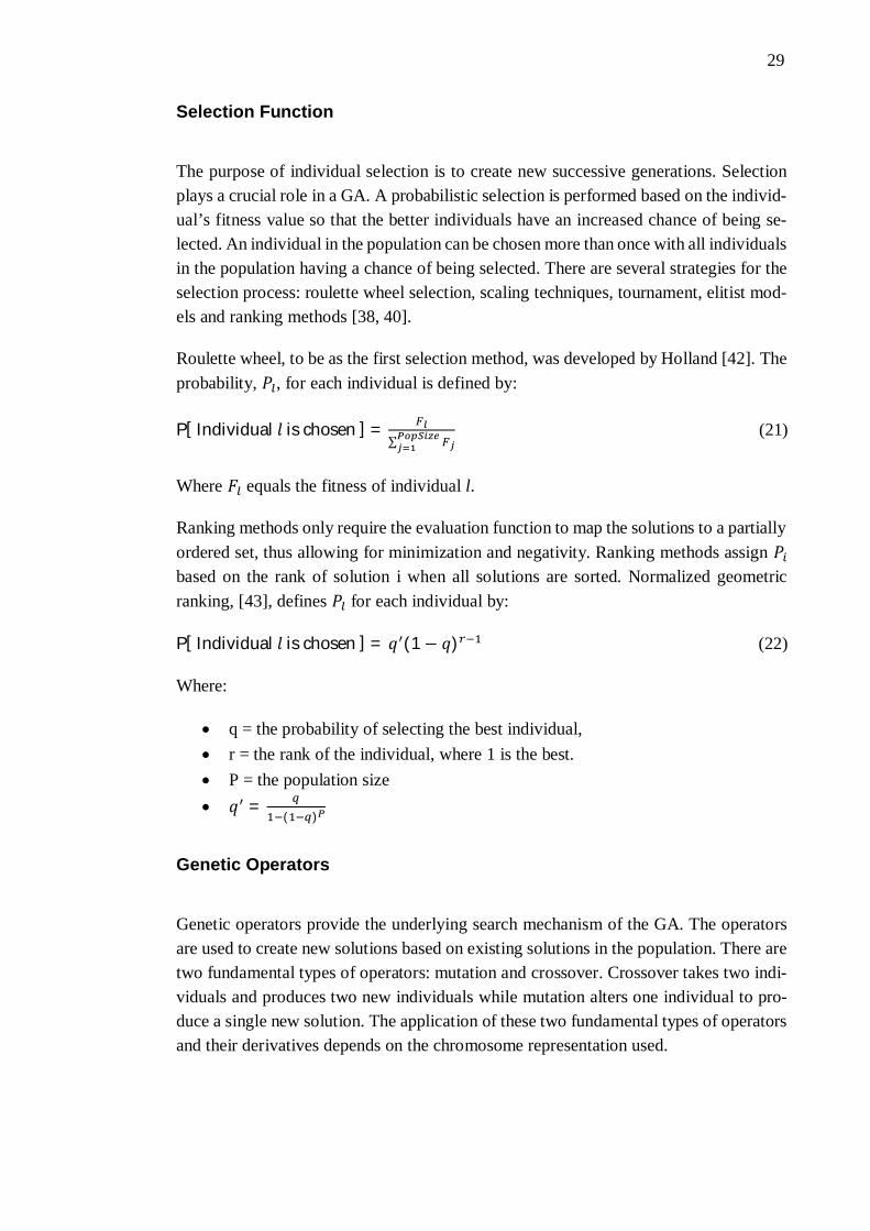
Roulette wheel, to be as the first selection method, was developed by Holland [42]. Theprobability, , for each individual is defined by:
P[Individual ischosen] =∑
(21)
Where equals the fitness of individual l.
Ranking methods only require the evaluation function to map the solutions to a partiallyordered set, thus allowing for minimization and negativity. Ranking methods assignbased on the rank of solution i when all solutions are sorted. Normalized geometricranking, [43], defines for each individual by:
P[Individual ischosen] = (1− ) (22)
Where:
· q = the probability of selecting the best individual,· r = the rank of the individual, where 1 is the best.· P = the population size· =
( )
Genetic Operators
Genetic operators provide the underlying search mechanism of the GA. The operatorsare used to create new solutions based on existing solutions in the population. There aretwo fundamental types of operators: mutation and crossover. Crossover takes two indi-viduals and produces two new individuals while mutation alters one individual to pro-duce a single new solution. The application of these two fundamental types of operatorsand their derivatives depends on the chromosome representation used.

30
Initialization, Termination, Evaluation Function
An initial population must be created for the GA at the beginning. The most commonmethod is to generate individuals for the entire population randomly. However, sinceGA can iteratively improve existing individuals, the beginning population can be storedas potentially useful solutions, with the remaining randomly generated individuals inthe population.
According to [44], “The GA moves from generation to generation selecting and repro-ducing parents until a termination criterion is met. The most often used stopping crite-rion is a specified maximum number of generation. Another termination strategy in-volves population convergence criteria. In general, as will force much of the entire pop-ulation to converge to a single solution.” Alternatively, a target value for the evaluationmeasure can be established based on some arbitrary threshold.
Fitness functions of many forms can be used in a GA, subject to the minimal require-ments that the function can map the population into a partially ordered set.
31
3. DIGITAL INTEGRATOR DESIGN
In this thesis, an optimal digital integrator is designed step by step. This filter is expectedapproximately to fulfill all the specifications mentioned in chapter 1. It is a multi-crite-rion design problem as there are specific requirements for both magnitude and phaseresponses. To this end, several design methods are combined.
Firstly, the choice of starting point filter has a great influence to the further optimization.Its design strategy varies depending on what integration algorithms are employed. Thestarting point filter is carefully selected by referring to the design specification and con-straints mentioned in Section 1.2. There are three proposed approaches that we couldchoose to create a starting point filter.
Secondly, optimized filter is obtained by applying optimization algorithms to thestarting point filter, GA optimization method is used in this thesis.
After the optimal filter is derived, several filter structures are proposed to illustrate thesuitability and stability of the desired filter with fixed point arithmetic. The frequencyresponses, as well as the corresponding filter structures, will be presented graphically.Group delay and time domain responses are compared with the specified criteria.
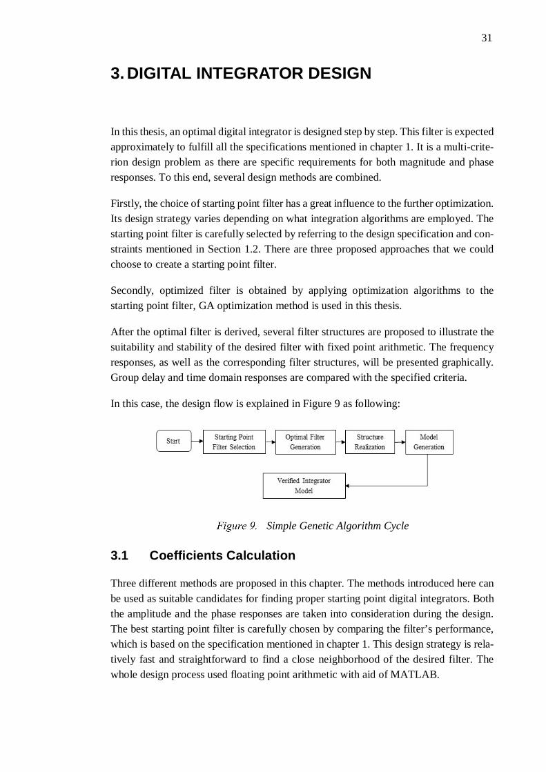
In this case, the design flow is explained in Figure 9 as following:
3.1 Coefficients Calculation
Three different methods are proposed in this chapter. The methods introduced here canbe used as suitable candidates for finding proper starting point digital integrators. Boththe amplitude and the phase responses are taken into consideration during the design.The best starting point filter is carefully chosen by comparing the filter’s performance,which is based on the specification mentioned in chapter 1. This design strategy is rela-tively fast and straightforward to find a close neighborhood of the desired filter. Thewhole design process used floating point arithmetic with aid of MATLAB.
Simple Genetic Algorithm Cycle
32
3.1.1 Starting Point Filter Design
In this section, several integrators are designed. All the filters’ coefficients use floatingpoint arithmetic, the finite word length effects are not taken into consideration at thisdesign stage.
Direct Designed Integrators
For direct design method, the most important thing is to find out proper input parame-ters. It is mainly a process of trial and try. In the beginning, very simple data are used,then according to the output coefficients and filter performance, corresponding modifi-cations can be done.
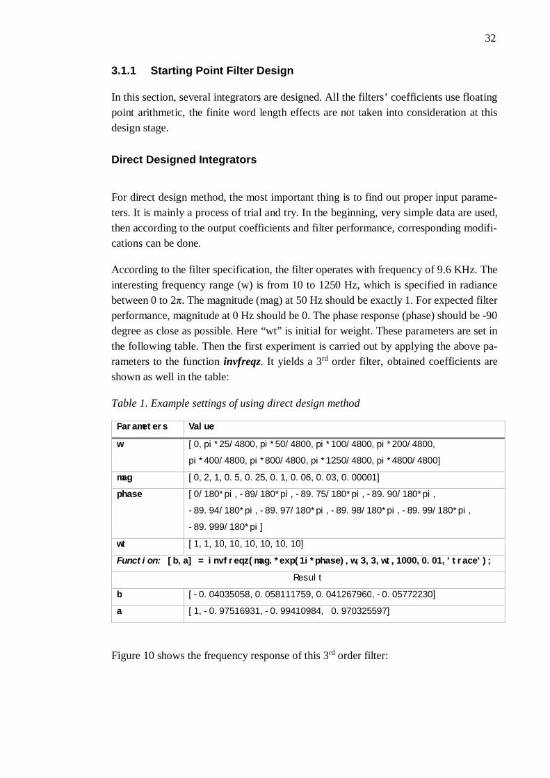
According to the filter specification, the filter operates with frequency of 9.6 KHz. Theinteresting frequency range (w) is from 10 to 1250 Hz, which is specified in radiancebetween 0 to 2π. The magnitude (mag) at 50 Hz should be exactly 1. For expected filterperformance, magnitude at 0 Hz should be 0. The phase response (phase) should be -90degree as close as possible. Here “wt” is initial for weight. These parameters are set inthe following table. Then the first experiment is carried out by applying the above pa-rameters to the function invfreqz. It yields a 3rd order filter, obtained coefficients areshown as well in the table:
Table 1. Example settings of using direct design method
Parameters Value
w [0,pi*25/4800,pi*50/4800,pi*100/4800,pi*200/4800,
pi*400/4800,pi*800/4800,pi*1250/4800,pi*4800/4800]
mag [0,2,1,0.5,0.25,0.1,0.06,0.03,0.00001]
phase [0/180*pi,-89/180*pi,-89.75/180*pi,-89.90/180*pi,
-89.94/180*pi,-89.97/180*pi,-89.98/180*pi,-89.99/180*pi,
-89.999/180*pi]
wt [1,1,10,10,10,10,10,10]
Function: [b,a] = invfreqz(mag.*exp(1i*phase),w,3,3,wt,1000,0.01,'trace');
Result
b [-0.04035058,0.058111759,0.041267960,-0.05772230]
a [1,-0.97516931,-0.99410984, 0.970325597]
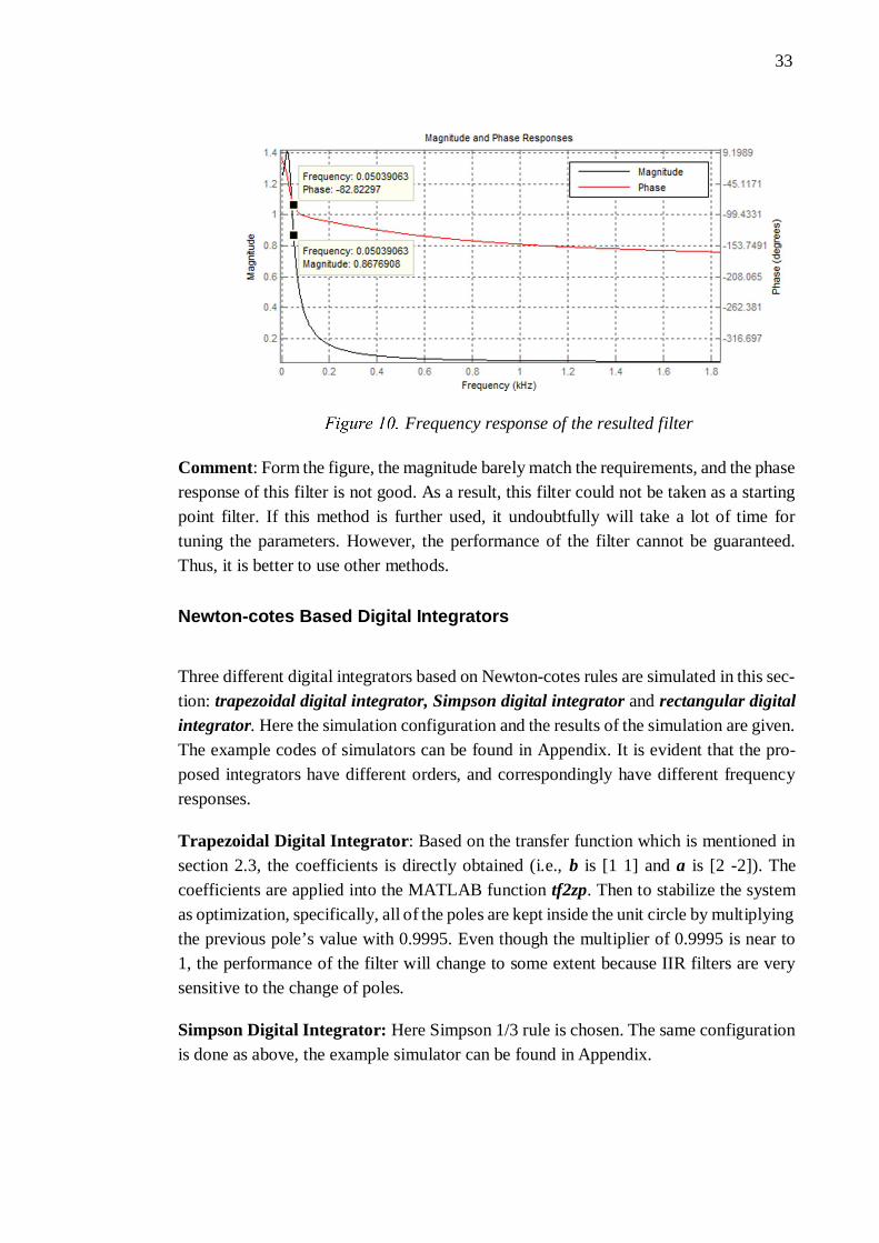
Figure 10 shows the frequency response of this 3rd order filter:
33
Comment: Form the figure, the magnitude barely match the requirements, and the phaseresponse of this filter is not good. As a result, this filter could not be taken as a startingpoint filter. If this method is further used, it undoubtfully will take a lot of time fortuning the parameters. However, the performance of the filter cannot be guaranteed.Thus, it is better to use other methods.
Newton-cotes Based Digital Integrators
Three different digital integrators based on Newton-cotes rules are simulated in this sec-tion: trapezoidal digital integrator, Simpson digital integrator and rectangular digitalintegrator. Here the simulation configuration and the results of the simulation are given.The example codes of simulators can be found in Appendix. It is evident that the pro-posed integrators have different orders, and correspondingly have different frequencyresponses.
Trapezoidal Digital Integrator: Based on the transfer function which is mentioned insection 2.3, the coefficients is directly obtained (i.e., b is [1 1] and a is [2 -2]). Thecoefficients are applied into the MATLAB function tf2zp. Then to stabilize the systemas optimization, specifically, all of the poles are kept inside the unit circle by multiplyingthe previous pole’s value with 0.9995. Even though the multiplier of 0.9995 is near to1, the performance of the filter will change to some extent because IIR filters are verysensitive to the change of poles.
Simpson Digital Integrator: Here Simpson 1/3 rule is chosen. The same configurationis done as above, the example simulator can be found in Appendix.
Frequency response of the resulted filter
34
Rectangular Digital Integrator: By analyzing the transfer function, we get the coeffi-cients as following and by the same means to apply the coefficients to MATLAB func-tions.
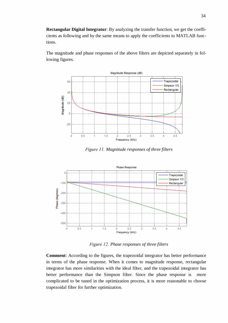
The magnitude and phase responses of the above filters are depicted separately in fol-lowing figures.
Comment: According to the figures, the trapezoidal integrator has better performancein terms of the phase response. When it comes to magnitude response, rectangularintegrator has more similarities with the ideal filter, and the trapezoidal integrator hasbetter performance than the Simpson filter. Since the phase response is morecomplicated to be tuned in the optimization process, it is more reasonable to choosetrapezoidal filter for further optimization.
Magnitude responses of three filters
Phase responses of three filters

35
Next, in order to get a better filter, either optimization methods needs to be applied, orthe filter’s order needs to be increased if the trapezoidal integrator was chosen as thestarting point filter. Based on this conclusion, we increased the order of trapezoidalintegrator by adding a notch near 0 Hz. The example simulator is given in Appendix.and the corresponding frequency response showed in Figure 11 proved our choice was
right.
Comment: After adding a notch, here this modified filter is called as candidate 1filter.This filter has not only good phase response but also excellent magnitude response. Asa result, this filter could be a superb choice for the starting point integrator.
Frequency response of trapezoidal integrator after adding a notch

36
Direct Design Based On the Frequency Response
Another fundamental digital integrator was derived by directly identifying the transferfunction, which corresponds to the given frequency response. In this case, the expectedmagnitude and phase response and are defined at first in specific frequency points.
Then the MATLAB function invfreqz is used to convert data into transfer function co-efficients. A simple case is introduced in Appendix to explain how it works:
Comment: By analyzing the above figure, it is evident that both magnitude and phaseresponse of the integrator is far away from the expectation of the desired filter. As aconclusion, even though further optimization methods could be used on the filter, itwould cost more time to choose this method to design the starting point filter than toselect the candidate 1 filter.
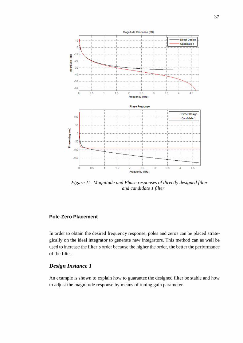
A comparison between the directly designed filter and candidate 1 filter is given inFigure 15. It is evident that candidate 1 filter has better performance than the directlydesigned filter.
Frequency response of directly designed filter
37
Pole-Zero Placement
In order to obtain the desired frequency response, poles and zeros can be placed strate-gically on the ideal integrator to generate new integrators. This method can as well beused to increase the filter’s order because the higher the order, the better the performanceof the filter.
Design Instance 1
An example is shown to explain how to guarantee the designed filter be stable and howto adjust the magnitude response by means of tuning gain parameter.
Magnitude and Phase responses of directly designed filterand candidate 1 filter

38
Here the original trapezoidal integrator is employed to illustrate how the pole-zeroplacement method works. Figure 14 shows the position of pole and zero of the trapezoi-dal integrator on z-plane.
Comment: As it is known, the filter is stable when all of the poles are inside the unitcircle. However, from the above figure, it 's hard to tell whether the poles are inside theunit circle or not. In order to guarantee the stability of the filter, the pole’s position needsto be adjusted. The same method mentioned in the section for trapezoidal integratordesign (program 1) in Appendix is utilized to make sure the position of poles.
Now the filter is stable. By adjusting the obtained gain value k, the magnitude responseof the filter at 50 Hz is tuned to be 1 (i.e., 0 dB). Figure 17 is the magnitude and phaseresponse of the modified first-order trapezoidal integrator obtained above. As the figureshows, it is clear that the magnitude response at 50 Hz is very close to 0 dB.
Pole- zero position of the original trapezoidal integrator
39
Design Instance 2
This example is for explaining how to utilize pole-zero placement to add a notch for afilter. According to Figure 17, the phase response of the first order trapezoidal integratorperforms well. However the magnitude response at 0 Hz is huge, which means that ifthere is a DC input, the output value of the filter will be saturated and would neverdecay. This result is not expected. Additionally, based on the specification, it is neededto minimize the magnitude response at 0 Hz. Therefore, it is necessary to add a notcharound 0 Hz, where the pole-zero placement method is utilized again.
A conjunct pair of zero and pole is added around 0 Hz, which will yield a 3 rd-order filter.What needs to be mentioned here is that the width of the notch affects the stability,impulse response and other performance of the filter. A concrete example is given inAppendix.
Frequency response of the modified first-order trapezoi-dal integrator
40
The new filter’s zero-pole-gain value are obtained after these operations. As is shownin Figure 18, all of the poles and zeros are quite near to the boundary of the unit circle.In other words, even though tiny changes of the coefficients of the filter, the poles willhave great chances to be outside the unit circle, and the filter will be unstable corre-spondingly. As a result, in order to get a better filter, the coefficients or the positions ofpoles and zeros need to be adjusted carefully.
Figure 19 gives a comparison between this 3rd-order integrator and the previous candi-date 1 filter.
Summary: this 3rd order filter is very similar to candidate 1 filter. In brief, this filter isdeveloped from the basic trapezoidal filter, by means of adjusting the gain value and
Pole- zero position of the 3rd-order integrator
Magnitude response of 3rd-order integrator and the Candi-date 1 filter
41
adding a notch (or increase the order of the filter). That is, we used the basic designmethod as well as pole-zero placement to develop a 3rd order starting point filter. As aresult, it is not very easy to develop a well-performed filter by purely using only onedesign method. We should take all of the specifications into account and take advantageof all of the methods we have to make the filter as better as possible.
3.1.2 Coefficients Optimization
Above section mentioned that the higher of the filter’s order, the greater possibility ofgetting a better performance. In this section, a genetic algorithm is proposed to solve theoptimization problems in search of better 3rd and 4th order filters. Both the 3rd and 4th
order filters are derived by using the pole-zero placement method above. The 4th orderfilter is obtained by adding a new notch around 0 Hz on the GA optimized 3rd ordercandidate 1 filter, which has very good frequency response and impulse response if thefitness function is well defined.
The GA optimization was implemented with the aid of MATLAB. In this case, 5 user-defined MATLAB functions are created, which are: GA_optimization, Selection,Fit_Evaluation, Mutation, and Crossover. For confidential consideration, this thesiswould not show the whole subroutines. But in the rest of the section, the main aspectsassociated with the algorithm are discussed with details.
GA_optimization Function
This is the primary function of GA optimization method in this thesis, which runs thesimulated evolution. The primary call to this function is given by the followingMATLAB command:
[BestValue,best,bestfit]=GA_optimization(pSize,pGen,N,Fs,pCross,pMutation,mutStr)
Output parameters
· BestValue is the best solution string, i.e. final solution,· Best is group of each BestValue from every generation during optimization,· Bestfit is group of fitness value from every generation.
Input parameters
· pSize is the size of the population· pGen is number of iterations· N is the order of the filter· Fs is the sampling frequency· pCross is crossover possibility
42
· pMutation is a mutation possibility· mutStr is strength of mutation
Population Initialization
The purpose of population initialization is to provide the GA_optimization a startingpoint filter. It is executed by using the method of pole-zero placement. The particularoperation to place the poles and zeros is based on the observation and analysis of pole-zero distribution (Figure 18), which is from a basic 3rd order filter.
Based on the pole-zero distribution graph, there are 3 steps to be done to determine thestrategy of corresponding pole-zero placement.
Step 1: Find the general distributions of all zeros. From the graph we can see, there isone zero on the negative real axis, and other two on the positive real axis. The absolutevalues are all smaller than one but very near to the unit boundary. MATLAB functionrand can be used to generate the initial values of zeros.
Step 2: Find the general distributions of all poles. There is one pole right on the positivereal axis, which is quite near to the unit circle but smaller than 1. There are two poleswith very small angles, which is quite near to the real axis.
Step 3: Determine the variation interval for each variable (or the search space), includ-ing all zeros and poles as well as the scale value.
An example of how to generate new poles and zeros can be found in Appendix.
Termination Condition
The termination algorithm determines when to stop the simulated evolution and returnthe result population. GA_optimization checks the termination condition every gener-ation. The function will terminate either at specified generation or the optimal or maxgeneration when best individual case is found.
Selection Function
The selection function determines which of the individuals will survive and continue tothe next generation. The GA_optimization function calls the selection function eachgeneration after new population is created from the old one. The basic function call usedis:
[selectpop] = Selection(pop)
Where selectpop is the new population selected, input pop is the current population. Inour selection algorithm, both Ranking method and Roulette wheel are used. The former

43
one is to decide the choosing probability, the latter one is to choose the individualfrom the current population based on the choosing probability.
Fitness Function
The function is called from GA main fucntion to determine the fitness of each solutionstring generated during the search process. It is important to decide which performanceof the filter should be taken into account and how to evaluate it, that is, how to translatethe performance into quantifiable data. For example, the filter’s magnitude responses atinteresting frequency points are necessary to be represented and evaluated. In addition,phase response, group delay, impulse response and stability of the filter have to be takeninto consideration.
After the evaluated performance is decided, the priority of these factors needs to bedetermined. Furthermore, the metric standard, which determines what kind of data isuseful and what kind of data is bad has to be made. There should be significant differ-ences in the fitness values between the well performed and the badly performed filters.
Fitness function is called by GA_optimization twice during every generation. One is atthe beginning, and the other is at the end after the new generation was derived. Here isthe basic call of this function:
[fitness] = Fit_Evaluation(pop)
Where fitness is the fitness value for every individual of the current generation pop,which is the input to the function.
Mutation and Crossover Functions
Mutation is one of the operator functions of the GA, the other one is Crossover, both ofwhich provide the search mechanism for GA and create new solutions based on existingsolutions in the population. Mutation changes one individual’s value to produce a newsolution, which could be tuned by the mutation strength. Crossover takes twoindividuals’ value and provides two new individuals after corresponding operations.
The function call for Mutation is as follows:
[NewPop]=Mutation(OldPop,pMutation,mutStr)
Where OldPop is the current generation, pMutation is the mutation possibility for thegeneration and mutStr is the mutation strength for one picked individual. The newPopis the new generation with mutated individuals.
The Crossover function is similar:
44
[NewPop]=CrossOver(OldPop,pCross,opts)
Where OldPop is the current generation, pCross is the crossover possibility for thegeneration and opts is the option for different crossover strategy. In this thesis, we usemulti-point and equally crossover algorithms. The newPop is the new generation ofmutated individuals.
3.1.3 Design Example
In this section, a detailed explanation of the designing and optimization process is given.It is based on the real experiments by optimizing the 3rd and 4th ordered integrators.
Starting Point Filter Generating
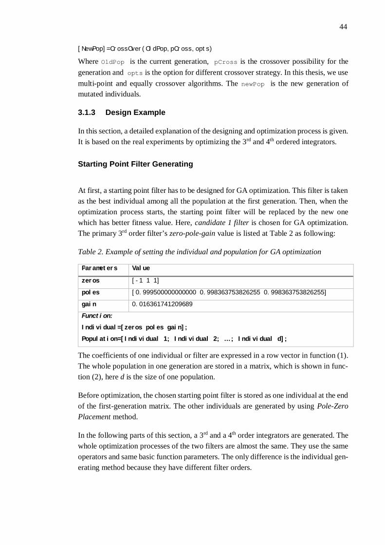
At first, a starting point filter has to be designed for GA optimization. This filter is takenas the best individual among all the population at the first generation. Then, when theoptimization process starts, the starting point filter will be replaced by the new onewhich has better fitness value. Here, candidate 1 filter is chosen for GA optimization.The primary 3rd order filter’s zero-pole-gain value is listed at Table 2 as following:
Table 2. Example of setting the individual and population for GA optimization
Parameters Value
zeros [-1 1 1]
poles [0.999500000000000 0.998363753826255 0.998363753826255]
gain 0.016361741209689
Function:
Individual=[zeros poles gain];
Population=[Individual 1; Individual 2; … ; Individual d];
The coefficients of one individual or filter are expressed in a row vector in function (1).The whole population in one generation are stored in a matrix, which is shown in func-tion (2), here d is the size of one population.
Before optimization, the chosen starting point filter is stored as one individual at the endof the first-generation matrix. The other individuals are generated by using Pole-ZeroPlacement method.
In the following parts of this section, a 3rd and a 4th order integrators are generated. Thewhole optimization processes of the two filters are almost the same. They use the sameoperators and same basic function parameters. The only difference is the individual gen-erating method because they have different filter orders.
45
In order to create a new 3rd order filter, the first step is to observe the pole and zerodistributions. According to Figure 18, all of the three poles are very close to the positiveaxis of the unit circle. Two zeros are near or on the positive real axis, and the rest one ison or close to the negative real axis of the unit circle. From above analysis, a new ran-dom 3rd order integrator is generated by Pole-Zero Placement method, and the code isshown in Program 8 in Appendix.
That’s how new individuals are created in GA optimization. After this optimization,better 3rd order integrator can be obtained with well-defined fitness function. If the op-timization results are not satisfactory, more times of iterations are need for the optimi-zation until a best filter is found.
Based on the optimized 3rd order integrator, a 4th order integrator is generated by addinga notch exactly at 0 Hz. An example is shown in Program 9 in Appendix:
Since a notch is directly added at 0 Hz, the notch angle is 0, there is no need to thinkabout the conjunct pair of the new zero and pole. That’s why the filter’s order is onlyincreased from 3 to 4 but not 5. All of the poles are at the positive part of the unit circle,and they are very close to the unit border. For the zeros, there are 3 of them at the positivepart on the unit circle, the other one is on the negative side. According to this conclusion,new filters for 4th order filter optimization can be created, the code is given in Program10 in Appendix.
When the starting point filter and the population for optimization are ready, the GAoptimization Process can be started.
3rd order filter optimization
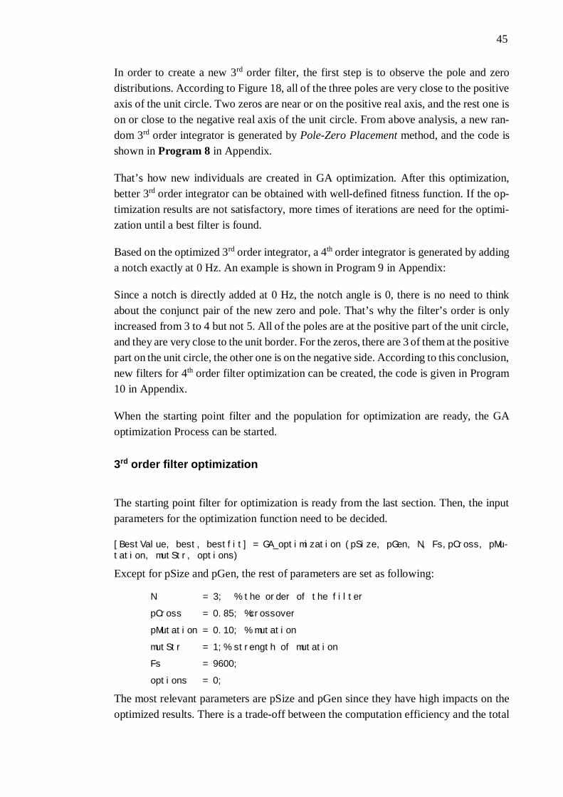
The starting point filter for optimization is ready from the last section. Then, the inputparameters for the optimization function need to be decided.
[BestValue, best, bestfit] = GA_optimization (pSize, pGen, N, Fs,pCross, pMu-tation, mutStr, options)
Except for pSize and pGen, the rest of parameters are set as following:
N = 3; % the order of the filter
pCross = 0.85; %crossover
pMutation = 0.10; % mutation
mutStr = 1;% strength of mutation
Fs = 9600;
options = 0;
The most relevant parameters are pSize and pGen since they have high impacts on theoptimized results. There is a trade-off between the computation efficiency and the total

46
optimization time. If pSize and pGen are huge, even though more optimization resultscould be found, the time that the whole optimization process will take will be longercorrespondingly. That’s why different parameter pairs of pSize and pGen are used fortesting in this case.
Table X shows the optimized individuals obtained during the optimization process withdifferent input values of pSize and pGen. It is obvious that the bigger pSize and pGenare, the longer the whole optimization process is. It is necessary to select a proper pairof pSize and pGen for the further optimization. That’s also the point of this experiment.
Table 3. Optimization results for different input pairs of pSize and pGen
pSize pGen Optimized Individuals
20 100 7
30 100 6
40 100 4
20 300 14
30 300 13
40 300 19
20 500 13
30 500 12
40 500 11
Comment: Finally, the number of pGen is set to be 300. When pGen is too small(pGen=100), there are not enough optimized results. When pGen is big (pGen=500), theoptimization does not converge any longer. When pGen=300, reasonable number ofoptimized individuals are obtained, and it takes shorter optimization time thanpGen=500.

47
The optimization process is plotted to show the variations in fitness values when thegenerations are evolving. Figure 20 depicts the differences in the fitness values tuningprocess with different pSize numbers.
Comment: According to above figures, the optimization results were not stable whenpSize was small. When pSize changed to be bigger, the optimization results tended tobe more reasonable. In account to optimization efficiency, it is a better choice to setpSize as 30.
(a)
(b)
(c)Variation in fitness values through generations with pSize
numbers of a) 20, b) 30 and c) 40
48
Performance Test
Even though the optimization method has been chosen, it is not very easy to select asuitable filter by simply adopting the GA optimization functions. One reason is that theinput parameters of the GA functions should be appropriately chosen, for the purposeof getting good optimization result without taking too much computation time. On theother hand, not all of the optimization results are valid since the fitness function couldnot take all of the performance factors into account for evaluation. And sometimes theoptimized results deviate from the primary filter coefficients too much that the resultednew filter is not an integrator any more. That’s why additional functional tests are stillneeded after optimization.
The following is an explanation about how to validate the optimization results.
According to the GA functions, all of the results are stored in a matrix, in which everyrow is a set of coefficients consist of zeros, poles and the gain factor of a filter. Thelatest optimized result is stored in the first row of the matrix. For most cases, the firstrow of the matrix could be taken as the best-optimized result among all of the results.However, sometimes it doesn’t work since the fitness function could not evaluate thefilter adequately. Then the following tests are needed for further selection of the bestfilter coefficients.
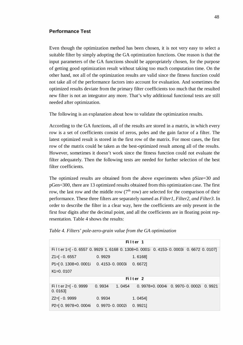
The optimized results are obtained from the above experiments when pSize=30 andpGen=300, there are 13 optimized results obtained from this optimization case. The firstrow, the last row and the middle row (7th row) are selected for the comparison of theirperformance. These three filters are separately named as Filter1, Filter2, and Filter3. Inorder to describe the filter in a clear way, here the coefficients are only present in thefirst four digits after the decimal point, and all the coefficients are in floating point rep-resentation. Table 4 shows the results:
Table 4. Filters’ pole-zero-grain value from the GA optimization
Filter 1
Filter1=[-0.6557 0.9929 1.6168 0.1308+0.0001i 0.4153-0.0003i 0.6672 0.0107]
Z1=[-0.6557 0.9929 1.6168]
P1=[0.1308+0.0001i 0.4153-0.0003i 0.6672]
K1=0.0107
Filter 2
Filter2=[-0.9999 0.9934 1.0454 0.9978+0.0004i 0.9970-0.0002i 0.99210.0163]
Z2=[-0.9999 0.9934 1.0454]
P2=[0.9978+0.0004i 0.9970-0.0002i 0.9921]
49
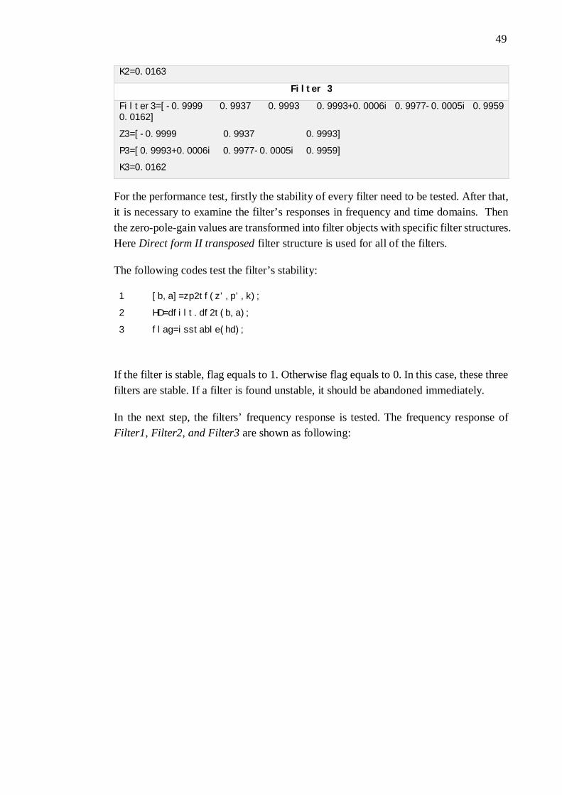
K2=0.0163
Filter 3
Filter3=[-0.9999 0.9937 0.9993 0.9993+0.0006i 0.9977-0.0005i 0.99590.0162]
Z3=[-0.9999 0.9937 0.9993]
P3=[0.9993+0.0006i 0.9977-0.0005i 0.9959]
K3=0.0162
For the performance test, firstly the stability of every filter need to be tested. After that,it is necessary to examine the filter’s responses in frequency and time domains. Thenthe zero-pole-gain values are transformed into filter objects with specific filter structures.Here Direct form II transposed filter structure is used for all of the filters.
The following codes test the filter’s stability:
1
2
3
[b,a]=zp2tf(z’,p’,k);
HD=dfilt.df2t(b,a);
flag=isstable(hd);
If the filter is stable, flag equals to 1. Otherwise flag equals to 0. In this case, these threefilters are stable. If a filter is found unstable, it should be abandoned immediately.
In the next step, the filters’ frequency response is tested. The frequency response ofFilter1, Filter2, and Filter3 are shown as following:
50
Comment: From Figure 21, Filter1 should be abandoned since both magnitude andphase responses of it are far worse than the other two filters. It also proves that a filterwith best fitness value is not the best choice.
Then Filter 2 and Filter 3 are compared again. Form above figures, it is obvious thatFilter 3 has better performance than Filter 2. But in some cases, it is very difficult todistinguish the two filters only by the frequency responses if the filters have very similarcoefficients, or even some coefficients of the filters are the same. Then it is necessaryto compare filters’ performance in particular frequency points. The following codes areshown as an example in Table 5:
(a)
(b)Frequency responses of Filter1, Filter2 and Filter3, a)
Magnitude Responses, b) Phase Responses

51
Table 5. Example codes showing how to test filter’s performance
Test magnitude response at 0 Hz and 50 Hz:
1
2
3
4
5
6
[h,w]=freqz(hd,9600,'whole');
resps=[abs(h)];
angles=angle(h)*180/pi;
w=w*4800/pi;
mag0=resps(1)% magnitude at 0 Hz
mag50=resps(51)% magnitude at 50 Hz
Test phase response at 50 Hz and 1000 Hz:
1
2
ang50=angles(51)% phase at 50 Hz
ang1000=angles(1001)% phase at 1000 Hz
Test group delay from 10 Hz to 1300 Hz with interval 10 Hz:
1 [grpd]=grpdelay(hd,[10:10:1300],9600);
All of the above tests are about filter performance in the frequency domain. The filter’sperformance in the time domain can be compared as well by checking out its impulseand step responses. An example is shown in Table 6:
Table 6. Example codes showing how to test the filter in the time domain
Test its impulse and step responses
1
2
3
4
Ts=1/9600;
sys=tf(b,a,Ts);
% impulse response
[impy,impt]=impulse(sys);
% step response
[stpy,stpt]=step(sys);
The results are visualized by plotting the response variances with time changing. Fig-ure 22 shows the impulse and step responses of Filter2 and Filter3.

52
Comment: According to the above figure, Filter3 has better performance than Filter2in both Impulse response and Step response. From the previous test, Filter3 also hasexcellent performance in the frequency domain. Thus, Filter3 is an excellent proof ofthe effectiveness of the GA optimization functions. In order to get even better filter,Filter3 can be further optimized by using the GA optimization again, or by increasingthe filter’s order and applying it to GA optimization.
In the following section, a 4th-order filter’s optimization is discussed.
4th order filter optimization
From last section, a very good 3rd order filter is obtained. Next a 4th order filter is gen-erated by adding a notch at 0 Hz. The newly generated filter has the following coeffi-cients:
z = [-0.9999 0.9937 0.9992 1.0000]p = [0.9992+0.0006i 0.9977-.0005i 0.9958 0.9940]k = 0.01623
This filter is taken to be starting point filter for the 4th order filter optimization. Then,the next optimization process is exactly the same as the 3rd order filter. According toprevious experience, pSize and pGen are separately set to be 30 and 300. Performance
Impulse and step responses of Filter2 and Filter3

53
tests are necessary after the optimization. After picking out the best result, it can bechosen to be the starting point filter for the next optimization round. After 3-5 times’iterations, a 4th order integrator with very good performance is obtained.
3.2 Structure Realization
After the optimization, the next step is to realize the filter with a suitable filter structure.Several available structures have been introduced in Chapter 2. This section mainly dis-cusses important issues about how to select a right filter structure.
3.2.1 Available Structures
When fixed point arithmetic is employed, carefully choosing a suitable structure iscritical. Based on the structures mentioned in Chapter 2, basic filter structures can betaken into consideration at first. The following four figures show Direct Form structuresof this 4th order IIR filter. All of the structures are described in block diagrams andderived by the Simulink toolbox of MATLAB.
Direct Form I Structure:
Direct Form I of the 4th order IIR filter
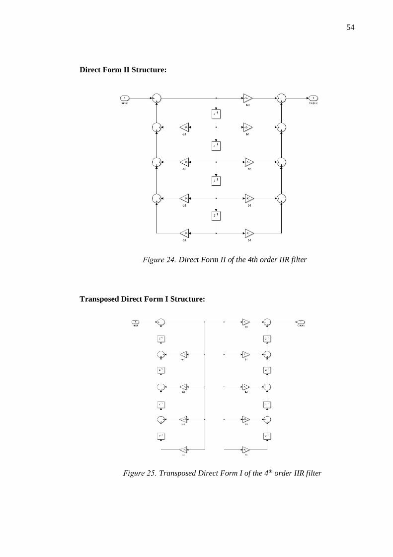
54
Direct Form II Structure:
Transposed Direct Form I Structure:
Direct Form II of the 4th order IIR filter
Transposed Direct Form I of the 4th order IIR filter
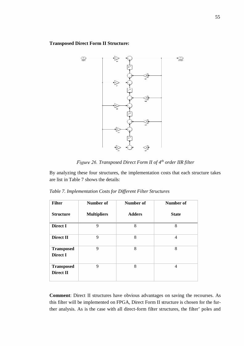
55
Transposed Direct Form II Structure:
By analyzing these four structures, the implementation costs that each structure takesare list in Table 7 shows the details:
Table 7. Implementation Costs for Different Filter Structures
Filter
Structure
Number of
Multipliers
Number of
Adders
Number of
State
Direct I 9 8 8
Direct II 9 8 4
TransposedDirect I
9 8 8
TransposedDirect II
9 8 4
Comment: Direct II structures have obvious advantages on saving the recourses. Asthis filter will be implemented on FPGA, Direct Form II structure is chosen for the fur-ther analysis. As is the case with all direct-form filter structures, the filter’ poles and
Transposed Direct Form II of 4th order IIR filter
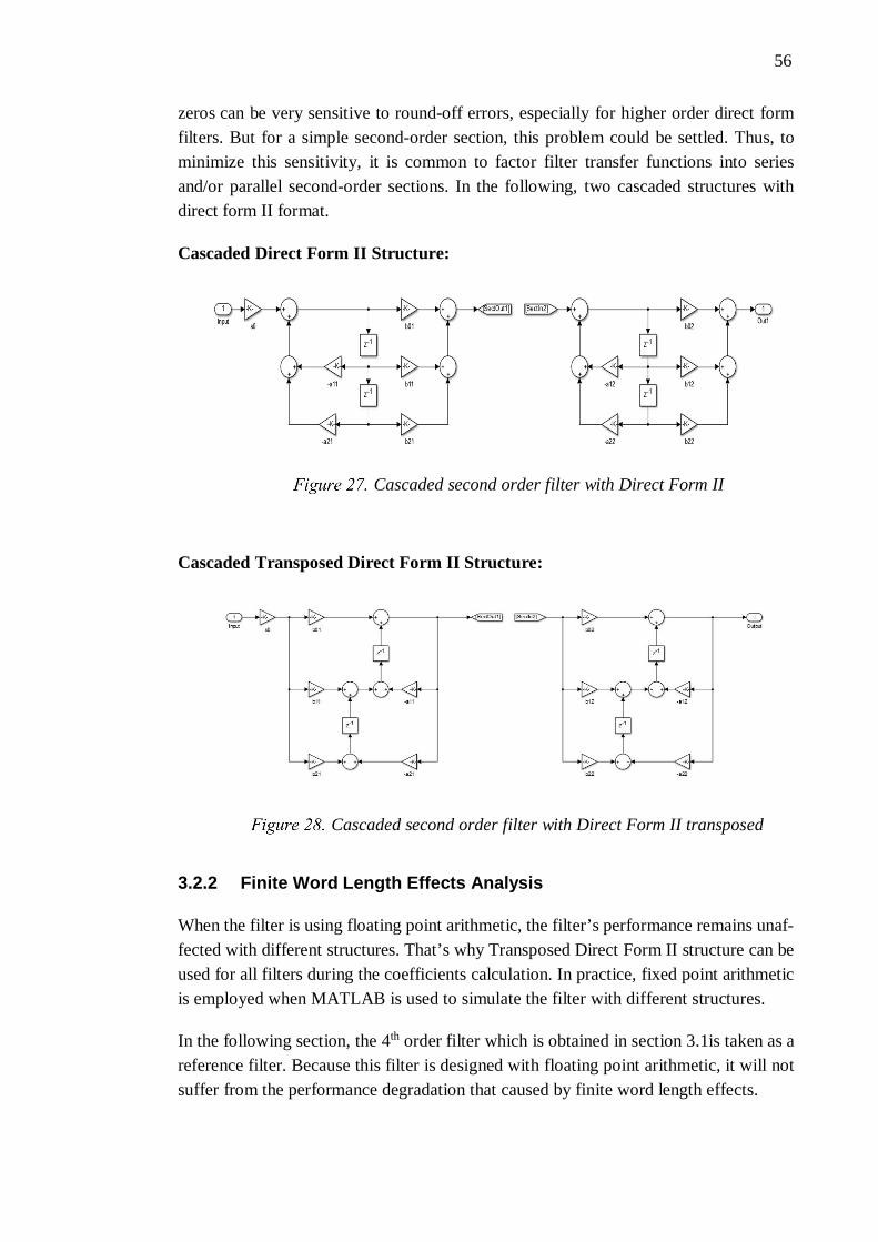
56
zeros can be very sensitive to round-off errors, especially for higher order direct formfilters. But for a simple second-order section, this problem could be settled. Thus, tominimize this sensitivity, it is common to factor filter transfer functions into seriesand/or parallel second-order sections. In the following, two cascaded structures withdirect form II format.
Cascaded Direct Form II Structure:
Cascaded Transposed Direct Form II Structure:
3.2.2 Finite Word Length Effects Analysis
When the filter is using floating point arithmetic, the filter’s performance remains unaf-fected with different structures. That’s why Transposed Direct Form II structure can beused for all filters during the coefficients calculation. In practice, fixed point arithmeticis employed when MATLAB is used to simulate the filter with different structures.
In the following section, the 4th order filter which is obtained in section 3.1is taken as areference filter. Because this filter is designed with floating point arithmetic, it will notsuffer from the performance degradation that caused by finite word length effects.
Cascaded second order filter with Direct Form II
Cascaded second order filter with Direct Form II transposed

57
Fixed Point Implementation
It is necessary to implement fixed point arithmetic on this 4th order IIR filter for filterrealization. When deciding fixed point format of the coefficients, the software and hard-ware limitations need to be taken into account. Technically, there is no limitation whenusing MATLAB to simulate with different fixed point formats. In practice, in order tosave the resources of the hardware, the best choice is to use as a short bit width as pos-sible. As the goal is to use reasonable bits to achieve good and acceptable filter perfor-mance when compared with the original filter in floating point format. To this end, thebit width of the coefficients is set to be 32 bits, which is the same length as the inputdata.
After the bit width is chosen, another important issue is how to distribute of the coeffi-cients’ integer and fractional bits. The fractional bits have a decisive effect on the dataprecision, and during calculation, proper integer bits could avoid overflow errors [ref-erence].
Taking the 4th order direct form II structure as example, Table 8 explains how to set thefilter’s fixed point format with specific structures with MATLAB:
Table 8. Example showing how to set filter’s fixed point attributes
Design direct form II filter object HD
HD=dfilt.df2(b,a);
Specify fixed point attributes and Word and Fractional length properties
HD.Arithmetic = 'fixed'; % Set fixed point precision
HD.Roundmode = 'floor'; % Set rounding strategy
HD.AccumWordLength = 64;
HD.StateWordLength = 64;
HD.CoeffWordLength = 32;
HD.InputWordLength = 32;
HD.OutputWordLength = 32;
HD.InputfracLength = 31;
HD.OutputfracLength = 31;
To ensure satisfactory fixed-point operation of the 4th order IIR filter, the following is-sues are necessary to be examined:
· Stability· Coefficient Quantization· Round-off Noise

58
Stability
The easiest way to check this attribute is using MATLAB function “isstable”:
flag = isstable(HD);
If the flag has value 1, the filter is stable. Otherwise, the filter is unstable, and the fixedpoint version is not suitable for the filter.
Then the stability of the Cascaded and Direct Form II structures are tested with 32 bitscoefficients format. These four filters are found stable.
There is another way to test the filter’s stability, which is related to the poles’ positionon pole/zero plot. Next section will discuss this issue.
Coefficient Quantization
The effect of quantization can be seen in the pole/zero plot. In fact, the issue of filter’sstability has to do with the denominator coefficients and correspondingly the poles, onthe pole/zero plot.
Pole-zero Deviation
For a quantized filter, the quantized coefficients will cause the displacement of polesand zeroes of the filter. Since the poles are very sensitive to a fixed point arithmetic, anda small change in the coefficients will cause the poles’ position changes, which mayyield significant performance changes correspondingly. In the following part, the dis-placement of poles and zeroes are discussed and analyzed by comparing different filterstructures with the ideal filter.
In Figure 29, this is the pole/zero plot of the filter in Direct Form II structure. The realpart of z-domain is zoomed in to show clearly how the poles and zeros’ positions deviatefrom the reference filter.
Pole-zero deviations
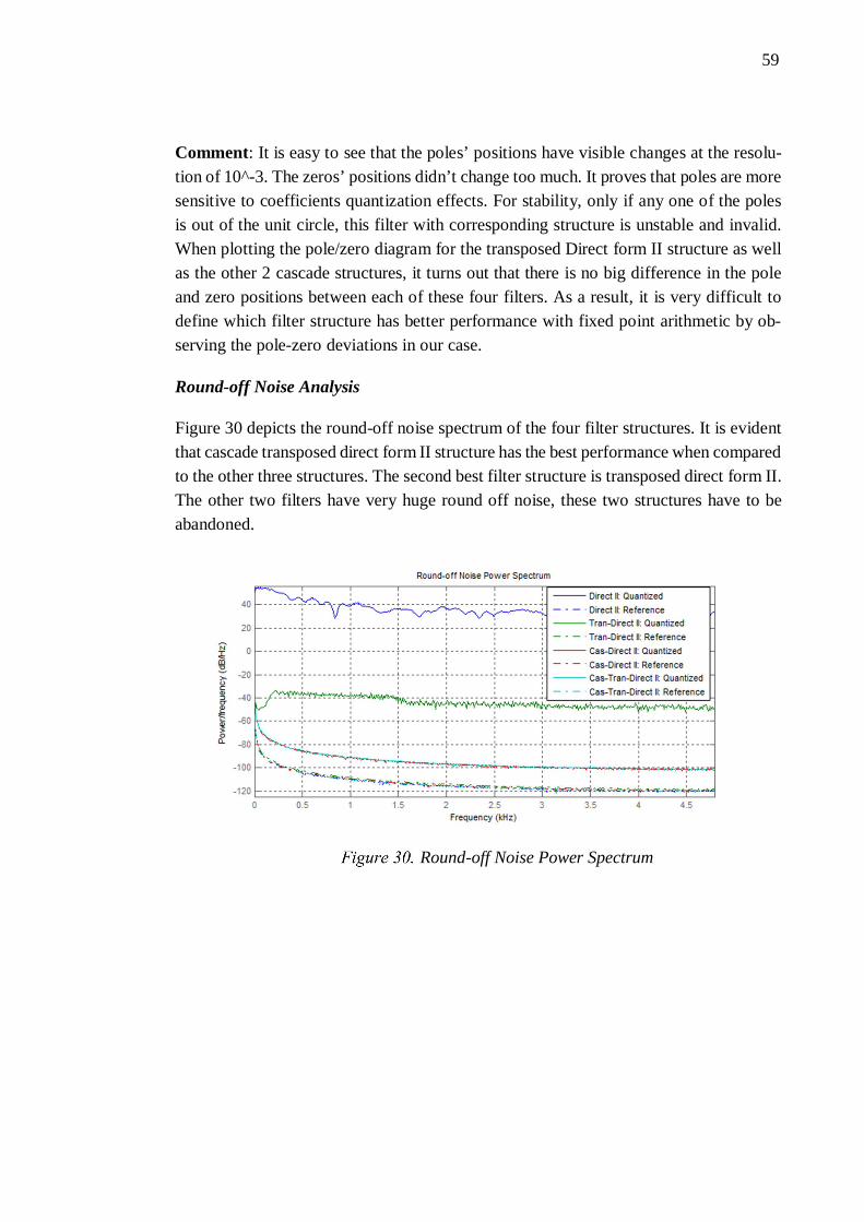
59
Comment: It is easy to see that the poles’ positions have visible changes at the resolu-tion of 10^-3. The zeros’ positions didn’t change too much. It proves that poles are moresensitive to coefficients quantization effects. For stability, only if any one of the polesis out of the unit circle, this filter with corresponding structure is unstable and invalid.When plotting the pole/zero diagram for the transposed Direct form II structure as wellas the other 2 cascade structures, it turns out that there is no big difference in the poleand zero positions between each of these four filters. As a result, it is very difficult todefine which filter structure has better performance with fixed point arithmetic by ob-serving the pole-zero deviations in our case.
Round-off Noise Analysis
Figure 30 depicts the round-off noise spectrum of the four filter structures. It is evidentthat cascade transposed direct form II structure has the best performance when comparedto the other three structures. The second best filter structure is transposed direct form II.The other two filters have very huge round off noise, these two structures have to beabandoned.
Round-off Noise Power Spectrum

60
Filtering Functionality Simulation
From the finite word length effect analysis, two appropriate filter structures are decided:Transposed Direct II and Cascade Second Order Section with Transposed DirectII structures. Finite word length effects are not the only issues that have to be carefullytreated when choosing the filter’s structure. The filter’s functionality is also an essentialfactor that needs to be checked.
In this section, the filtering functionality of these filters is simulated with the MATLABfunction “filter”:
Y=filter(HD,X);
It filters a vector of real or complex input data X through a fixed-point filter HD, pro-ducing filtered output data Y. The vectors X and Y have the same length. In this case,sinusoidal input X is generated in fixed point format s32.31, this signal is applied to thefilter function together with these two filter objects. Then the outputs Y is comparedwith the reference signal, which should be the ideal output result. Figure 31 shows thefiltering results.
Comment: It is obvious that filter with cascade structure has excellent output resultwhile the transposed direct II filter has very bad output results. Its output signal deviatesfrom the reference signal significantly.
This chapter gives a complete explanation of the process of how to design an integratorwith MATLAB. Based on all the facts, the filter structure can be decided to be CascadeSecond Order Section Transposed Direct II.
Filtering Functionality Simulation
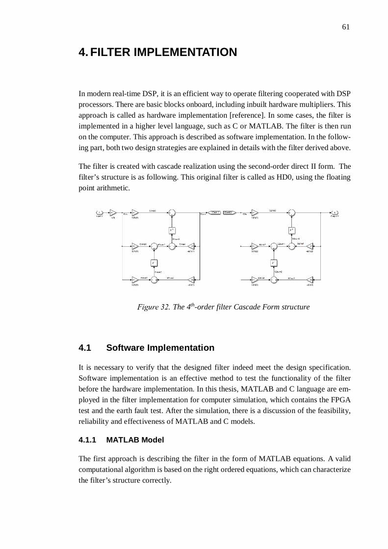
61
4. FILTER IMPLEMENTATION
In modern real-time DSP, it is an efficient way to operate filtering cooperated with DSPprocessors. There are basic blocks onboard, including inbuilt hardware multipliers. Thisapproach is called as hardware implementation [reference]. In some cases, the filter isimplemented in a higher level language, such as C or MATLAB. The filter is then runon the computer. This approach is described as software implementation. In the follow-ing part, both two design strategies are explained in details with the filter derived above.
The filter is created with cascade realization using the second-order direct II form. Thefilter’s structure is as following. This original filter is called as HD0, using the floatingpoint arithmetic.
4.1 Software Implementation
It is necessary to verify that the designed filter indeed meet the design specification.Software implementation is an effective method to test the functionality of the filterbefore the hardware implementation. In this thesis, MATLAB and C language are em-ployed in the filter implementation for computer simulation, which contains the FPGAtest and the earth fault test. After the simulation, there is a discussion of the feasibility,reliability and effectiveness of MATLAB and C models.
4.1.1 MATLAB Model
The first approach is describing the filter in the form of MATLAB equations. A validcomputational algorithm is based on the right ordered equations, which can characterizethe filter’s structure correctly.
The 4th-order filter Cascade Form structure

62
This model must be capable of filtering both floating point and fixed point data. It is aneasy way to design firstly the floating point filtering part, and then add fixed point arith-metic to the model. Since fixed point precision affects a lot of the filtering performance.It is necessary to guarantee that the model with floating point can work properly beforefixed point arithmetic is implemented.
Floating Point Filtering
This section mainly focuses on how to create right ordered equations for the MATLABmodel. Before deciding the equations, the filter’s coefficients are initialized accordingly.
Figure 32 shows the filter’ block diagram, with each section realized using a standardbi-quad structure. Here, section 1 is taken as an example to illustrate the algorithm forgenerating the right equations. The corresponding sets of difference equations are asfollows. For section2, the equations should be the same order as in section1.
1
2
3
4
5
6
7
8
9
S1in=x*s(0);
S1out= S1in+S1sum0;
S1ma1=S1out*(-S1a1);
S1mb1=S1in*S1b1;
S1sum1=S1ma1+S1mb1;
S1sum0=S1sum1+S1sum2;
S1ma2=S1out*(-S1a2);
S1mb2=S1in*S1b2;
S1sum2=S1mb2+S1ma2;
Here a proposed function named as “filter_matlab” is used to represent the MATLABmodel. This model is a m-file function with input and output parameters. The basic waythat this model deals with signals is like the following, (details cannot be narrated)
y(n) = filter_matlab (x(n), option)
Where y(n) is the filtering output vector or matrix, x(n) is the input signal in a matrixform. The option is used for choosing the mode of the filter, which means using filteringoperation or not, and it has values of either 1 or 0.
Computability Test
The values of all the coefficients in this model now are in floating points. For the originalfilter HD0, MATLAB function “filter” is used to execute the filtering operations. Whilefor the MATLAB model, the filtering function is realized by directly applying the inputsignal to the function. The testing strategy is to use the same input signal for both filtersand then compare the outputs of them. The operations are following:
Out1= filter(HD0, X);

63
Out2= filter_matlab (X, 1);
Where Out1 and Out2 represent the filtering outputs, X(notation) is the sinusoidal input.It turns out that Out1 exactly equals to Out2, which proves that the MATLAB model iscomputable and functions well.
Fixed Point Filtering
After the computability test, the basic MATLAB model is verified to be functional. Thenext step is to add the fixed point arithmetic on the basic model. Appropriate data pre-cision of the filter needs to be decided by means of several tests and analysis. It is obvi-ous that if more bits are used when implementing fixed point arithmetic, the more pre-cise the filter would be. However, with the hardware resource limitation under consid-eration, the input and output precision are decided to be s32.31.
In this case, the word-length of all coefficients are set to be 32 bits, as same as the inputand output data. Since the value of the coefficients varies in relatively broad range, cor-respondingly the fractional part length of coefficients varies as well. Then, how tochoose the proper fixed point representation for the intermediate variables becomes aprimary problem. An appropriate method is to assess the effects of finite word lengthon the filter performance and tune the fixed point precision.
The filter’s performance is evaluated by means of noise simulation. In general, integra-tors can have stability problems with zero input with some noise, which will result inoutput with DC levels due to rounding errors. The DC levels sometimes even go quitehigh. This happens mainly when there is no signal from the Rogowski coil. The mainreason for doing noise test is to check whether the integrator generates DC output ornot, and if it does, how much the DC output appears to be.
During the test, noise input is applied as a training signal to simulate the filter withdifferent coefficient precisions. By comparing and analyzing the output data, the fixedpoint representation of the coefficients is finally decided. It is necessary to tune carefullyand select the coefficients’ precision, a very good choice would yield smallest or evenno DC output when small noise input signal is processed by the filter. Figure 33 showsthe DC output with the final precision that be chosen. It is evident that the filter canavoid visible noise interrupts. There will not be significant DC level in the output, forboth noise signals with huge or tiny amplitudes.
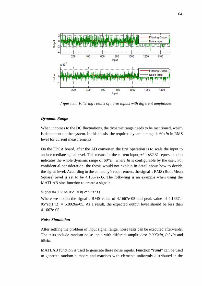
64
Dynamic Range
When it comes to the DC fluctuations, the dynamic range needs to be mentioned, whichis dependent on the system. In this thesis, the required dynamic range is 60xIn in RMSlevel for current measurements.
On the FPGA board, after the AD converter, the first operation is to scale the input toan intermediate signal level. This means for the current input, +/-1 s32.31 representationindicates the whole dynamic range of 60*In, where In is configurable by the user. Forconfidential consideration, the thesis would not explain in detail about how to decidethe signal level. According to the company’s requirement, the signal’s RMS (Root MeanSquare) level is set to be 4.1667e-05. The following is an example when using theMATLAB sine function to create a signal:
signal=4.1667e-05* sin(2*pi*f*t)
Where we obtain the signal’s RMS value of 4.1667e-05 and peak value of 4.1667e-05*sqrt (2) = 5.8926e-05. As a result, the expected output level should be less than4.1667e-05.
Noise Simulation
After settling the problem of input signal range, noise tests can be executed afterwards.The tests include random noise input with different amplitudes: 0.005xIn, 0.5xIn and60xIn.
MATLAB function is used to generate these noise inputs. Function “rand” can be usedto generate random numbers and matrices with elements uniformly distributed in the
Filtering results of noise inputs with different amplitudes
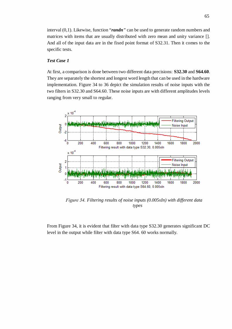
65
interval (0,1). Likewise, function “randn” can be used to generate random numbers andmatrices with items that are usually distributed with zero mean and unity variance [].And all of the input data are in the fixed point format of S32.31. Then it comes to thespecific tests.
Test Case 1
At first, a comparison is done between two different data precisions: S32.30 and S64.60.They are separately the shortest and longest word length that can be used in the hardwareimplementation. Figure 34 to 36 depict the simulation results of noise inputs with thetwo filters in S32.30 and S64.60. These noise inputs are with different amplitudes levelsranging from very small to regular.
From Figure 34, it is evident that filter with data type S32.30 generates significant DClevel in the output while filter with data type S64. 60 works normally.
Filtering results of noise inputs (0.005xIn) with different datatypes
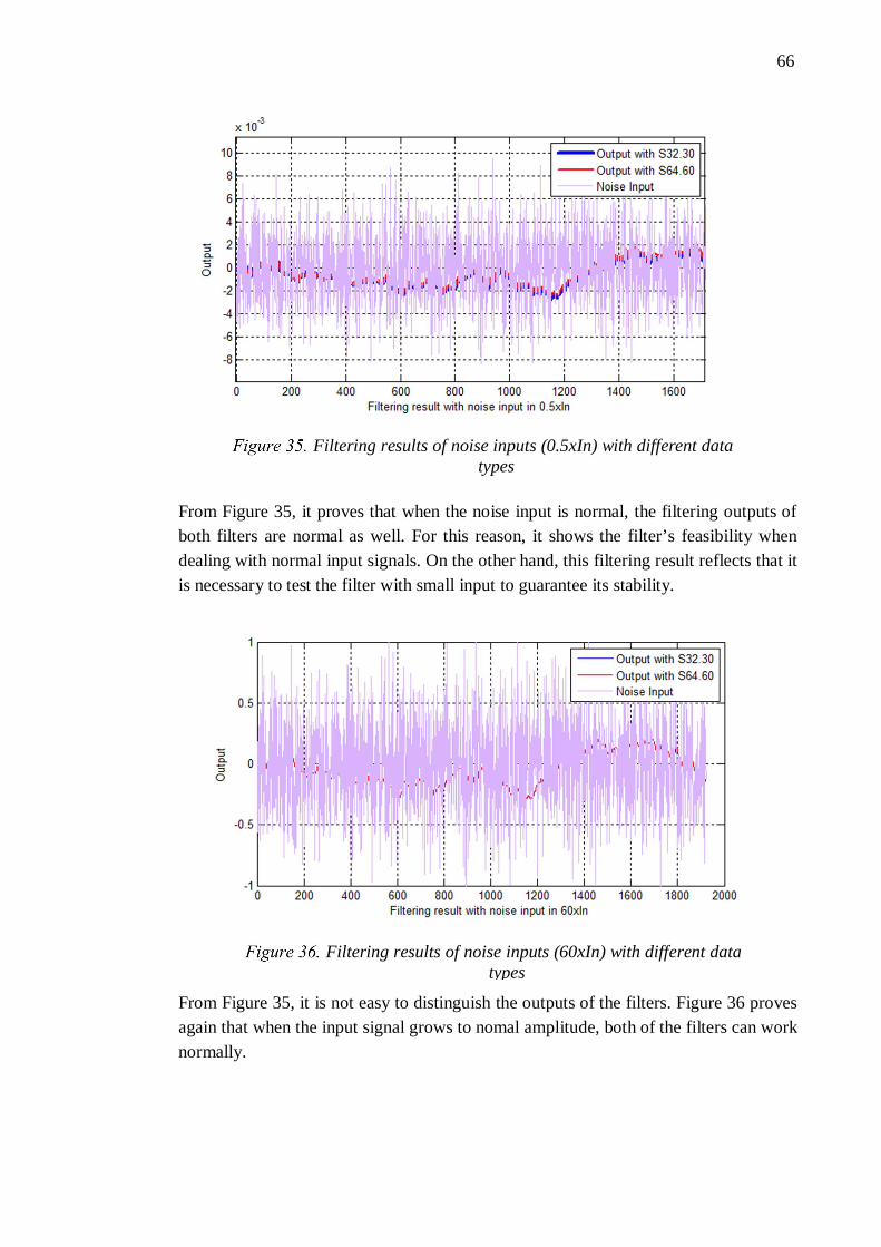
66
From Figure 35, it proves that when the noise input is normal, the filtering outputs ofboth filters are normal as well. For this reason, it shows the filter’s feasibility whendealing with normal input signals. On the other hand, this filtering result reflects that itis necessary to test the filter with small input to guarantee its stability.
From Figure 35, it is not easy to distinguish the outputs of the filters. Figure 36 provesagain that when the input signal grows to nomal amplitude, both of the filters can worknormally.
Filtering results of noise inputs (0.5xIn) with different datatypes
Filtering results of noise inputs (60xIn) with different datatypes
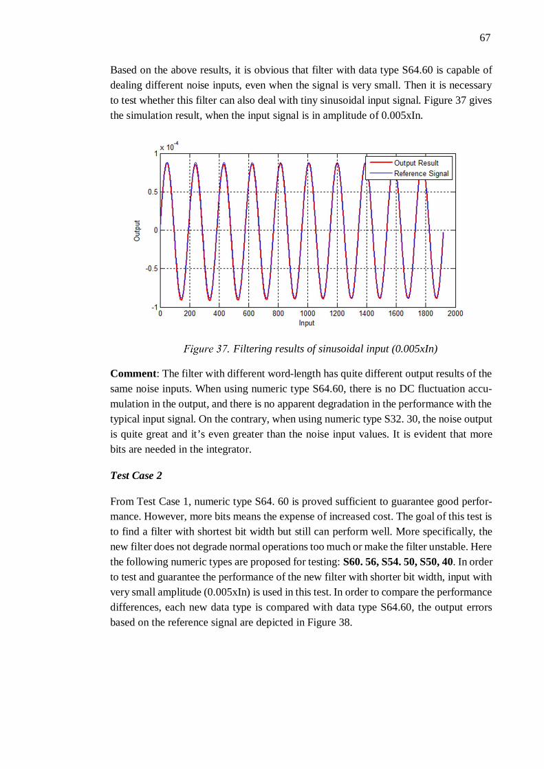
67
Based on the above results, it is obvious that filter with data type S64.60 is capable ofdealing different noise inputs, even when the signal is very small. Then it is necessaryto test whether this filter can also deal with tiny sinusoidal input signal. Figure 37 givesthe simulation result, when the input signal is in amplitude of 0.005xIn.
Comment: The filter with different word-length has quite different output results of thesame noise inputs. When using numeric type S64.60, there is no DC fluctuation accu-mulation in the output, and there is no apparent degradation in the performance with thetypical input signal. On the contrary, when using numeric type S32. 30, the noise outputis quite great and it’s even greater than the noise input values. It is evident that morebits are needed in the integrator.
Test Case 2
From Test Case 1, numeric type S64. 60 is proved sufficient to guarantee good perfor-mance. However, more bits means the expense of increased cost. The goal of this test isto find a filter with shortest bit width but still can perform well. More specifically, thenew filter does not degrade normal operations too much or make the filter unstable. Herethe following numeric types are proposed for testing: S60. 56, S54. 50, S50, 40. In orderto test and guarantee the performance of the new filter with shorter bit width, input withvery small amplitude (0.005xIn) is used in this test. In order to compare the performancedifferences, each new data type is compared with data type S64.60, the output errorsbased on the reference signal are depicted in Figure 38.
Filtering results of sinusoidal input (0.005xIn)

68
Figure 38 shows that except for the filter with data type of S50. 40, other filters per-formed well. This means that data type S50. 40 is not sufficient, in another word, eitherthe whole data bits or the fractional bits are not long enough. Then new numeric typesare proposed: S50. 45, S54. 43. The outputs of these three filters are presented in Figure
39.
Output error comparison of different data types
Output error comparisons of different data types

69
From the figure above, it is evident that numeric type S54.43 has awful filtering perfor-mance, even though with a longer bit width. This fact indicates that the primary reasonfor performance degradation is that the fractional bits are not long enough. From this,the numeric type S50.45 could be a real choice. For more precision consideration andseveral more functional experiments, the filter’s numeric type is finally decided to beS53.45.
4.1.2 C-Language Model
The second proposed approach is to realize the filter by C language. C model is benefi-cial than MATLAB in the sense to directly make VHDL from C, without the aid ofMathworks C to VHDL tool.
The fixed-point representation of the filter has been carefully chosen for filter realizationwith MATLAB. However, the descriptions of the same coefficients and intermediatedata of the filter are different in C model. In MATLAB model, the fixed-point algo-rithms are designed by using the built-in MATLAB Fixed-Point Toolbox. MATLABfunctions such as “fi”, “fimath” are used to construct and characterize the fixed-pointnumeric objects directly from the floating-point numeric type. When referring to the Clanguage model, the data is in the appearance of integer numeric type, which needs tobe transformed again from the fixed-point data. For a fixed point number A, the corre-sponding integer type A_int is derived by following operation:
A_int=A.int;
Multi-Precision Library -- GMP Implementation
In C language model, there are several variables that need more than 64 bits after thearithmetic operations (mainly multiplication). It is obvious basic integer types in C lan-guage are not sufficient for this case, a new method to represent the filter’s variables isneeded. For this purpose, GNU Multiple Precision (GMP) Arithmetic Library is intro-duced. It is a free library for arbitrary precision arithmetic, operating on signed integers,rational numbers and floating-point numbers [43].
The integer arithmetic functions provided by GMP library is also called as “mpz”. Thereare about 150 arithmetic and logic functions in this category [43]. GMP integers arestored in objects of type mpz_t, and the GMP integer functions start with the prefixmpz_. In Table 9, integer A_int and GMP integer A_mpz are used to explain the basicoperations of GMP integer functions.
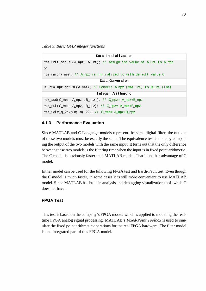
70
Table 9. Basic GMP integer functions
Data Initialization
mpz_init_set_si(A_mpz, A_int); // Assign the value of A_int to A_mpz
or
mpz_init(a_mpz); // A_mpz is initialized to with default value 0
Data Conversion
B_int= mpz_get_si(A_mpz); // Convert A_mpz (mpz int) to B_int (int)
Integer Arithmetic
mpz_add(C_mpz, A_mpz ,B_mpz ); // C_mpz= A_mpz+B_mpz
mpz_mul(C_mpz, A_mpz, B_mpz); // C_mpz= A_mpz+B_mpz
mpz_fdiv_q_2exp(m, m, 22); // C_mpz= A_mpz+B_mpz
4.1.3 Performance Evaluation
Since MATLAB and C Language models represent the same digital filter, the outputsof these two models must be exactly the same. The equivalence test is done by compar-ing the output of the two models with the same input. It turns out that the only differencebetween these two models is the filtering time when the input is in fixed point arithmetic.The C model is obviously faster than MATLAB model. That’s another advantage of Cmodel.
Either model can be used for the following FPGA test and Earth-Fault test. Even thoughthe C model is much faster, in some cases it is still more convenient to use MATLABmodel. Since MATLAB has built-in analysis and debugging visualization tools while Cdoes not have.
FPGA Test
This test is based on the company’s FPGA model, which is applied to modeling the real-time FPGA analog signal processing. MATLAB’s Fixed-Point Toolbox is used to sim-ulate the fixed point arithmetic operations for the real FPGA hardware. The filter modelis one integrated part of this FPGA model.
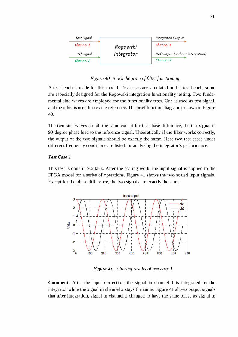
71
A test bench is made for this model. Test cases are simulated in this test bench, someare especially designed for the Rogowski integration functionality testing. Two funda-mental sine waves are employed for the functionality tests. One is used as test signal,and the other is used for testing reference. The brief function diagram is shown in Figure40.
The two sine waves are all the same except for the phase difference, the test signal is90-degree phase lead to the reference signal. Theoretically if the filter works correctly,the output of the two signals should be exactly the same. Here two test cases underdifferent frequency conditions are listed for analyzing the integrator’s performance.
Test Case 1
This test is done in 9.6 kHz. After the scaling work, the input signal is applied to theFPGA model for a series of operations. Figure 41 shows the two scaled input signals.Except for the phase difference, the two signals are exactly the same.
Comment: After the input correction, the signal in channel 1 is integrated by theintegrator while the signal in channel 2 stays the same. Figure 41 shows output signalsthat after integration, signal in channel 1 changed to have the same phase as signal in
Block diagram of filter functioning
Filtering results of test case 1
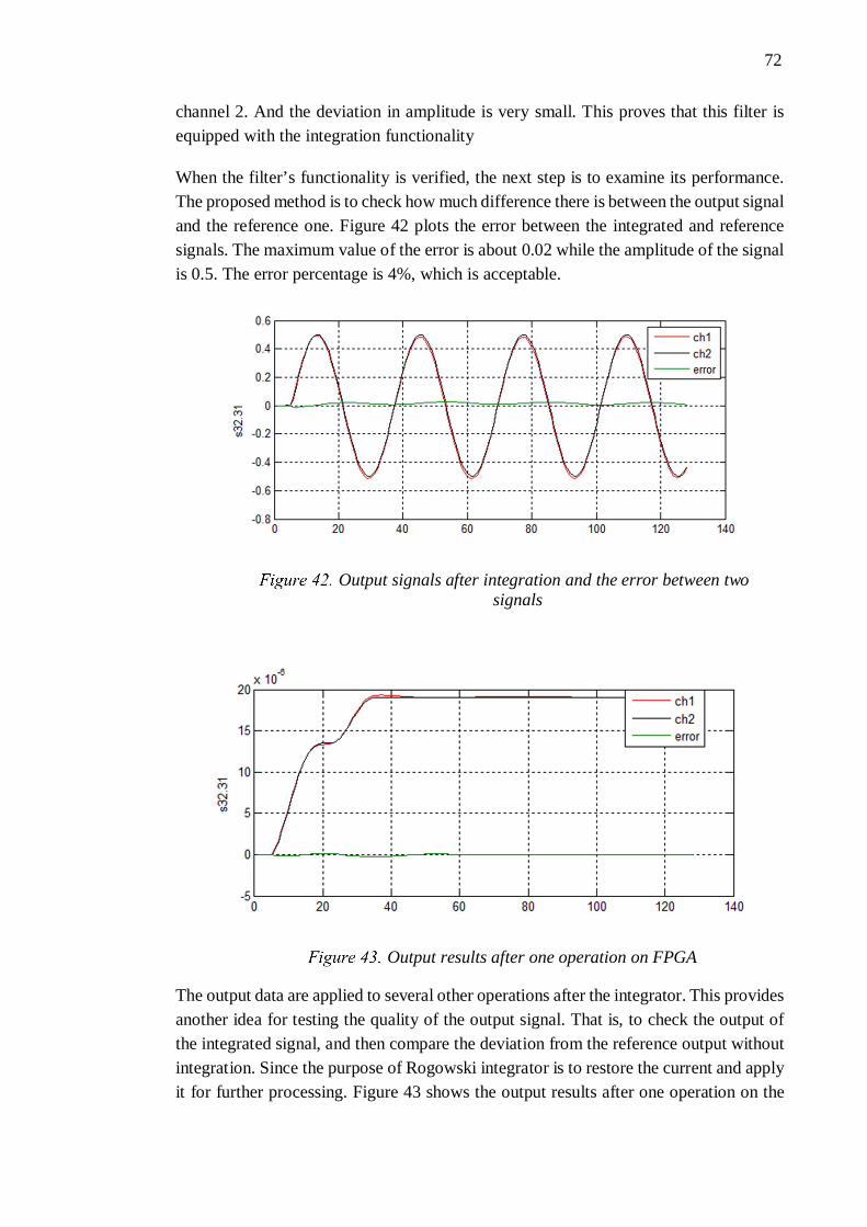
72
channel 2. And the deviation in amplitude is very small. This proves that this filter isequipped with the integration functionality
When the filter’s functionality is verified, the next step is to examine its performance.The proposed method is to check how much difference there is between the output signaland the reference one. Figure 42 plots the error between the integrated and referencesignals. The maximum value of the error is about 0.02 while the amplitude of the signalis 0.5. The error percentage is 4%, which is acceptable.
The output data are applied to several other operations after the integrator. This providesanother idea for testing the quality of the output signal. That is, to check the output ofthe integrated signal, and then compare the deviation from the reference output withoutintegration. Since the purpose of Rogowski integrator is to restore the current and applyit for further processing. Figure 43 shows the output results after one operation on the
Output results after one operation on FPGA
Output signals after integration and the error between twosignals
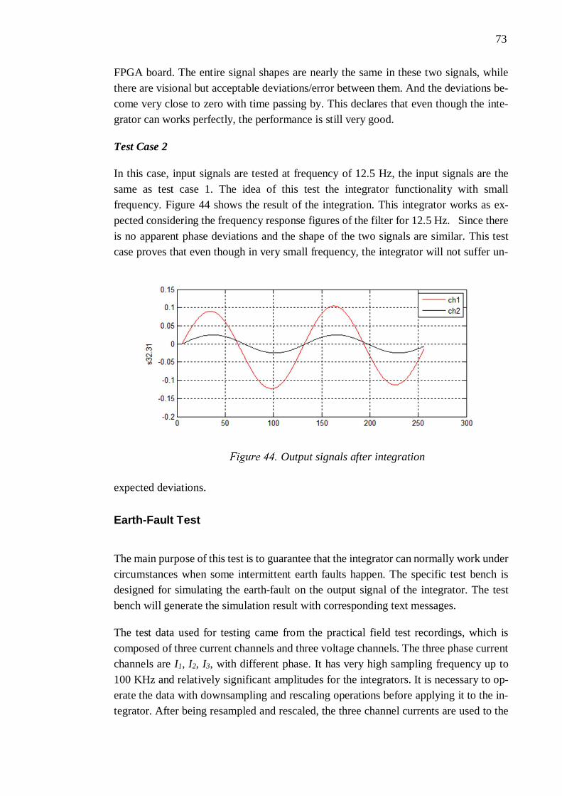
73
FPGA board. The entire signal shapes are nearly the same in these two signals, whilethere are visional but acceptable deviations/error between them. And the deviations be-come very close to zero with time passing by. This declares that even though the inte-grator can works perfectly, the performance is still very good.
Test Case 2
In this case, input signals are tested at frequency of 12.5 Hz, the input signals are thesame as test case 1. The idea of this test the integrator functionality with smallfrequency. Figure 44 shows the result of the integration. This integrator works as ex-pected considering the frequency response figures of the filter for 12.5 Hz. Since thereis no apparent phase deviations and the shape of the two signals are similar. This testcase proves that even though in very small frequency, the integrator will not suffer un-
expected deviations.
Earth-Fault Test
The main purpose of this test is to guarantee that the integrator can normally work undercircumstances when some intermittent earth faults happen. The specific test bench isdesigned for simulating the earth-fault on the output signal of the integrator. The testbench will generate the simulation result with corresponding text messages.
The test data used for testing came from the practical field test recordings, which iscomposed of three current channels and three voltage channels. The three phase currentchannels are I1, I2, I3, with different phase. It has very high sampling frequency up to100 KHz and relatively significant amplitudes for the integrators. It is necessary to op-erate the data with downsampling and rescaling operations before applying it to the in-tegrator. After being resampled and rescaled, the three channel currents are used to the
Output signals after integration
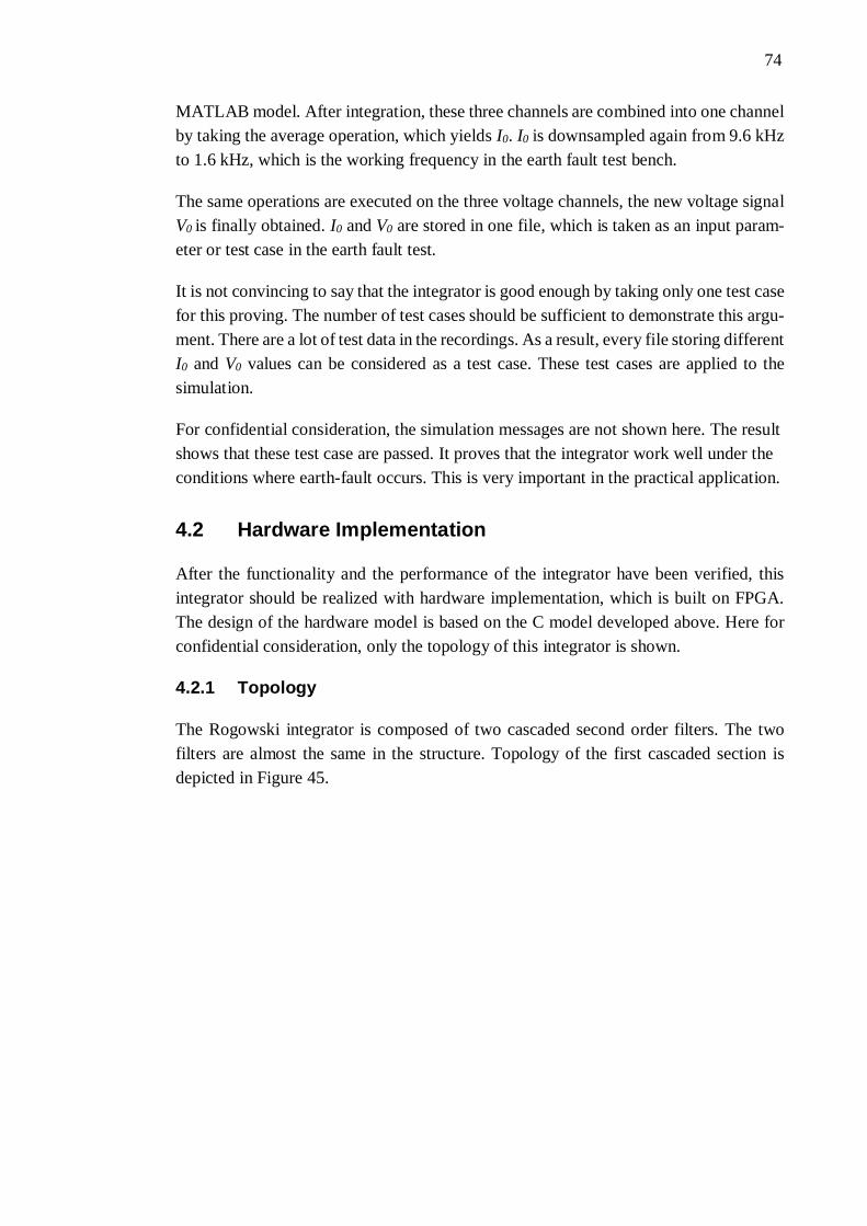
74
MATLAB model. After integration, these three channels are combined into one channelby taking the average operation, which yields I0. I0 is downsampled again from 9.6 kHzto 1.6 kHz, which is the working frequency in the earth fault test bench.
The same operations are executed on the three voltage channels, the new voltage signalV0 is finally obtained. I0 and V0 are stored in one file, which is taken as an input param-eter or test case in the earth fault test.
It is not convincing to say that the integrator is good enough by taking only one test casefor this proving. The number of test cases should be sufficient to demonstrate this argu-ment. There are a lot of test data in the recordings. As a result, every file storing differentI0 and V0 values can be considered as a test case. These test cases are applied to thesimulation.
For confidential consideration, the simulation messages are not shown here. The resultshows that these test case are passed. It proves that the integrator work well under theconditions where earth-fault occurs. This is very important in the practical application.
4.2 Hardware Implementation
After the functionality and the performance of the integrator have been verified, thisintegrator should be realized with hardware implementation, which is built on FPGA.The design of the hardware model is based on the C model developed above. Here forconfidential consideration, only the topology of this integrator is shown.
4.2.1 Topology
The Rogowski integrator is composed of two cascaded second order filters. The twofilters are almost the same in the structure. Topology of the first cascaded section isdepicted in Figure 45.
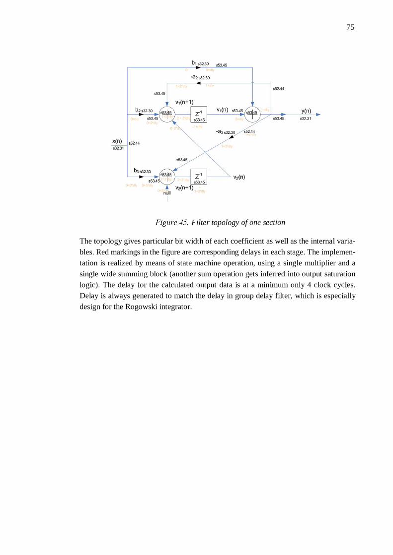
75
The topology gives particular bit width of each coefficient as well as the internal varia-bles. Red markings in the figure are corresponding delays in each stage. The implemen-tation is realized by means of state machine operation, using a single multiplier and asingle wide summing block (another sum operation gets inferred into output saturationlogic). The delay for the calculated output data is at a minimum only 4 clock cycles.Delay is always generated to match the delay in group delay filter, which is especiallydesign for the Rogowski integrator.
Filter topology of one section
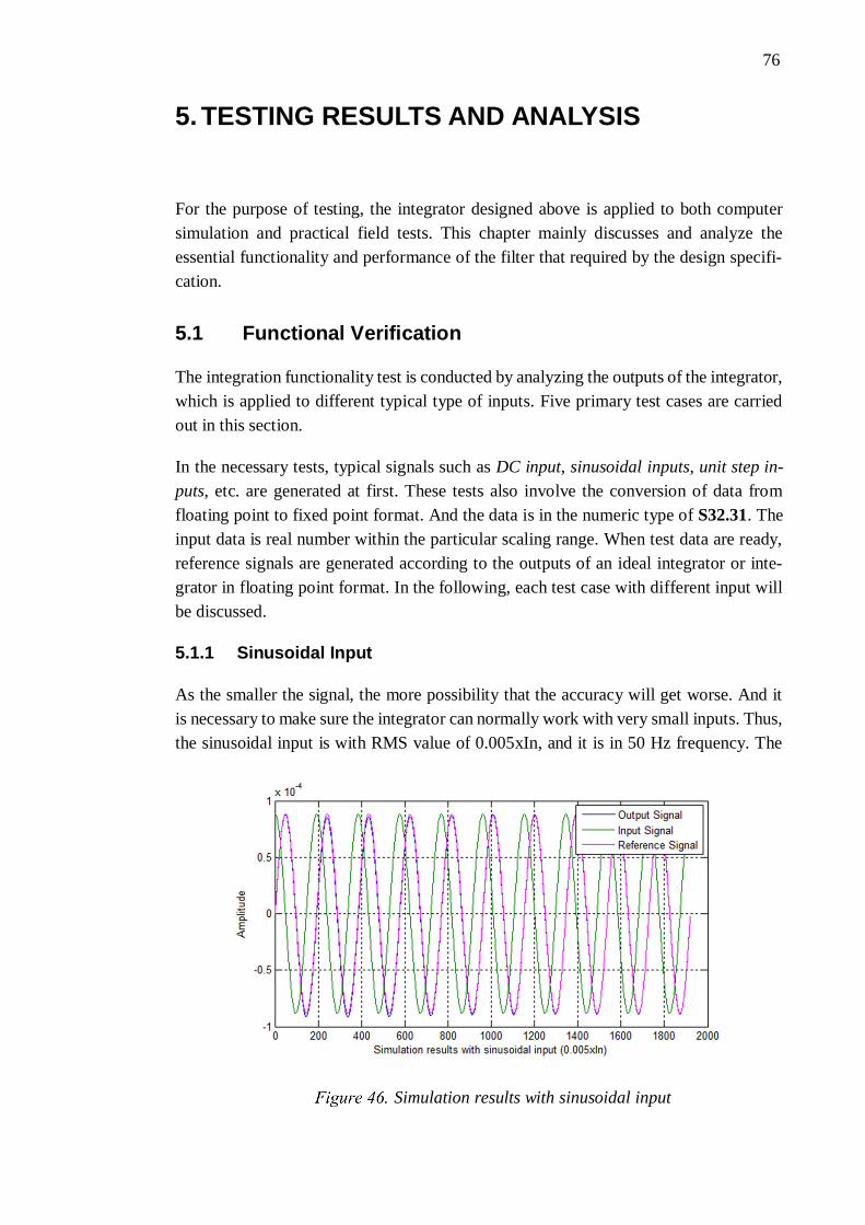
76
5. TESTING RESULTS AND ANALYSIS
For the purpose of testing, the integrator designed above is applied to both computersimulation and practical field tests. This chapter mainly discusses and analyze theessential functionality and performance of the filter that required by the design specifi-cation.
5.1 Functional Verification
The integration functionality test is conducted by analyzing the outputs of the integrator,which is applied to different typical type of inputs. Five primary test cases are carriedout in this section.
In the necessary tests, typical signals such as DC input, sinusoidal inputs, unit step in-puts, etc. are generated at first. These tests also involve the conversion of data fromfloating point to fixed point format. And the data is in the numeric type of S32.31. Theinput data is real number within the particular scaling range. When test data are ready,reference signals are generated according to the outputs of an ideal integrator or inte-grator in floating point format. In the following, each test case with different input willbe discussed.
5.1.1 Sinusoidal Input
As the smaller the signal, the more possibility that the accuracy will get worse. And itis necessary to make sure the integrator can normally work with very small inputs. Thus,the sinusoidal input is with RMS value of 0.005xIn, and it is in 50 Hz frequency. The
Simulation results with sinusoidal input

77
filtering result is compared with the original input signal as well the reference signal.Figure 46 depicts the comparison.
The figure shows that the filter integrated the input signal with -90-degree shift andalmost the same amplitude of the previous signal is kept. As in the specification, whenthe input signal is 50 Hz, the integrated result should exactly 1. The figure also provesthat the integrated signal is almost the same as the reference signal, even though, theinput is relatively small. This fact indicates that this integrator normally works even withtiny input signals.
5.1.2 DC Input
According to the specification, the integrator output should be zero with the DC inputto prevent the integrator windup. When designing the integrator in chapter 3, notcheswere explicitly added correctly at 0 Hz for this purpose. However in a practical imple-mentation, it is very difficult to realize excellent performance for quantization effects.Additionally, the filter’s magnitude response at 50 Hz should be 1, and then there willbe a very steep peak between these two frequency points. As a conclusion, the expectedoutput for a DC input may have fluctuates at the beginning, but it will decay to zero withtime passing.
In this test case, the input is still in the range of 0.005xIn to ensure the filter’s function-ality. Figure 47 shows the filtering result.
From the figure, the output has relative but acceptable fluctuate in the beginning. Withtime passing by, the output tended to be zero. It is very good to see that after 10000samples (9.6 kHz sampling frequency is used so that the period is about 1 second), theoutput is very close to 0. This test result proves again that the integrator normally works .
Simulation results with DC input
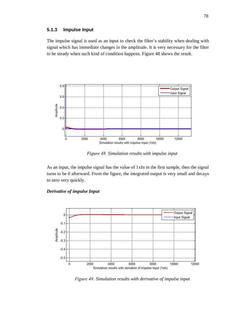
78
5.1.3 Impulse Input
The impulse signal is used as an input to check the filter’s stability when dealing withsignal which has immediate changes in the amplitude. It is very necessary for the filterto be steady when such kind of condition happens. Figure 48 shows the result.
As an input, the impulse signal has the value of 1xIn in the first sample, then the signalturns to be 0 afterward. From the figure, the integrated output is very small and decaysto zero very quickly.
Derivative of impulse Input
Simulation results with impulse input
Simulation results with derivative of impulse input
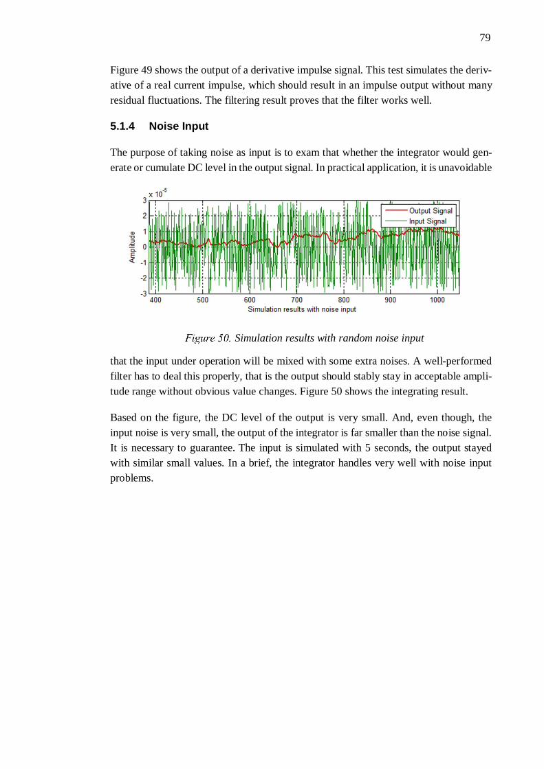
79
Figure 49 shows the output of a derivative impulse signal. This test simulates the deriv-ative of a real current impulse, which should result in an impulse output without manyresidual fluctuations. The filtering result proves that the filter works well.
5.1.4 Noise Input
The purpose of taking noise as input is to exam that whether the integrator would gen-erate or cumulate DC level in the output signal. In practical application, it is unavoidable
that the input under operation will be mixed with some extra noises. A well-performedfilter has to deal this properly, that is the output should stably stay in acceptable ampli-tude range without obvious value changes. Figure 50 shows the integrating result.
Based on the figure, the DC level of the output is very small. And, even though, theinput noise is very small, the output of the integrator is far smaller than the noise signal.It is necessary to guarantee. The input is simulated with 5 seconds, the output stayedwith similar small values. In a brief, the integrator handles very well with noise inputproblems.
Simulation results with random noise input
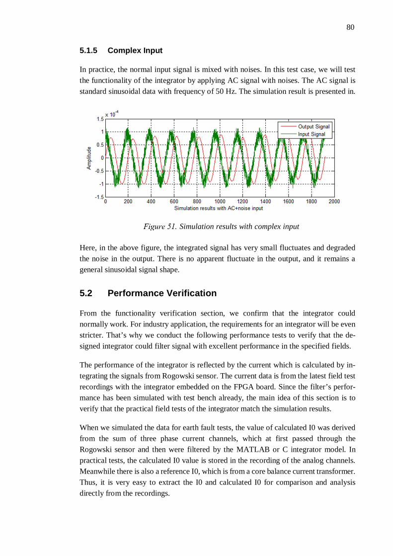
80
5.1.5 Complex Input
In practice, the normal input signal is mixed with noises. In this test case, we will testthe functionality of the integrator by applying AC signal with noises. The AC signal isstandard sinusoidal data with frequency of 50 Hz. The simulation result is presented in.
Here, in the above figure, the integrated signal has very small fluctuates and degradedthe noise in the output. There is no apparent fluctuate in the output, and it remains ageneral sinusoidal signal shape.
5.2 Performance Verification
From the functionality verification section, we confirm that the integrator couldnormally work. For industry application, the requirements for an integrator will be evenstricter. That’s why we conduct the following performance tests to verify that the de-signed integrator could filter signal with excellent performance in the specified fields.
The performance of the integrator is reflected by the current which is calculated by in-tegrating the signals from Rogowski sensor. The current data is from the latest field testrecordings with the integrator embedded on the FPGA board. Since the filter’s perfor-mance has been simulated with test bench already, the main idea of this section is toverify that the practical field tests of the integrator match the simulation results.
When we simulated the data for earth fault tests, the value of calculated I0 was derivedfrom the sum of three phase current channels, which at first passed through theRogowski sensor and then were filtered by the MATLAB or C integrator model. Inpractical tests, the calculated I0 value is stored in the recording of the analog channels.Meanwhile there is also a reference I0, which is from a core balance current transformer.Thus, it is very easy to extract the I0 and calculated I0 for comparison and analysisdirectly from the recordings.
Simulation results with complex input

81
There are different test cases since there are hundreds of recording files, and the fieldtests covered different kind of faults, we will mainly list several test cases with variousearth faults introduced. For each test case, the calculated I0 is analyzed by the followingthree performance issues:
· Accuracy· Transient State· Stable State
5.2.1 Solid Earth-Fault
At first, we analyze the test case where the solid earth-fault was interrupted. From Figure52, it is evident that the accuracy of the calculated I0 is very good since the two currentsignals overlap on each other relatively well.
Then the figure is zoomed in for more details about the transient and stable states. Thediagram in the below of Figure 52 depicts the transient state after the earth fault wasintroduced. As we could see, there are fluctuates in the calculated I0 signal but the am-plitude and phase of the current are almost the same as the reference signal. We couldrefer this condition to the Impulse Response simulation in section 5.1.3 since the tran-sient process is similar to the impulse response. In that simulation, the response at first
Simulation results with solid earth-fault
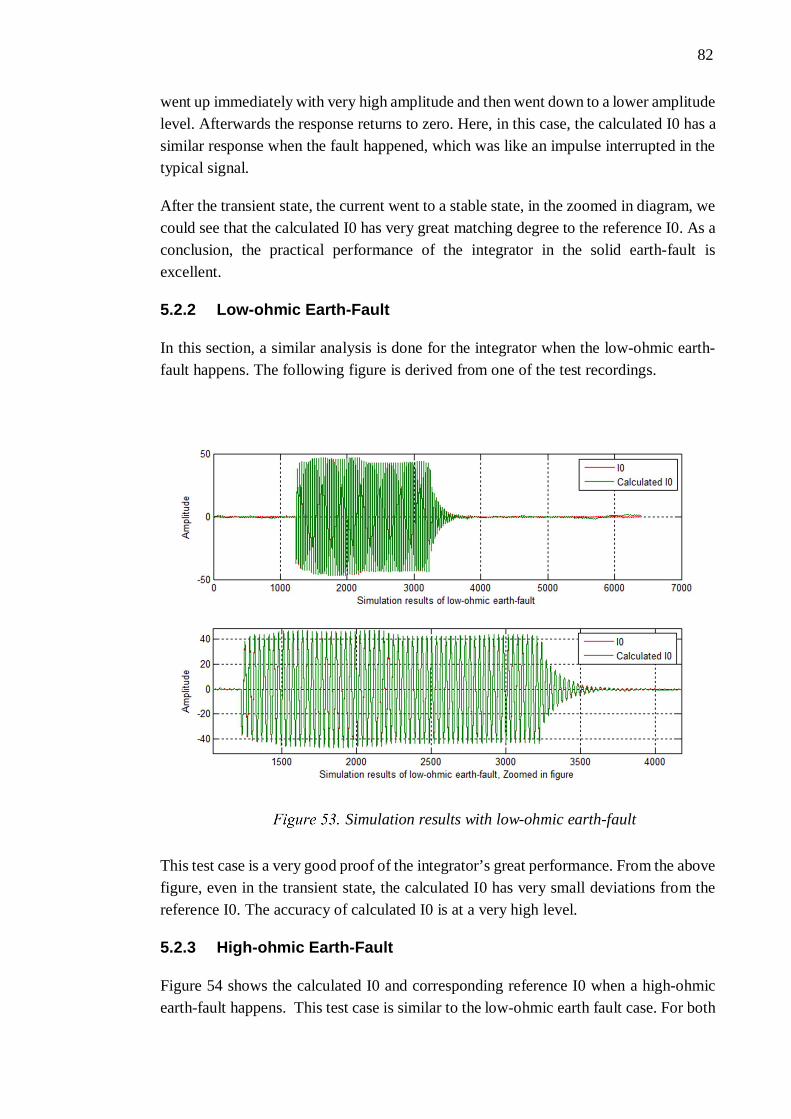
82
went up immediately with very high amplitude and then went down to a lower amplitudelevel. Afterwards the response returns to zero. Here, in this case, the calculated I0 has asimilar response when the fault happened, which was like an impulse interrupted in thetypical signal.
After the transient state, the current went to a stable state, in the zoomed in diagram, wecould see that the calculated I0 has very great matching degree to the reference I0. As aconclusion, the practical performance of the integrator in the solid earth-fault isexcellent.
5.2.2 Low-ohmic Earth-Fault
In this section, a similar analysis is done for the integrator when the low-ohmic earth-fault happens. The following figure is derived from one of the test recordings.
This test case is a very good proof of the integrator’s great performance. From the abovefigure, even in the transient state, the calculated I0 has very small deviations from thereference I0. The accuracy of calculated I0 is at a very high level.
5.2.3 High-ohmic Earth-Fault
Figure 54 shows the calculated I0 and corresponding reference I0 when a high-ohmicearth-fault happens. This test case is similar to the low-ohmic earth fault case. For both
Simulation results with low-ohmic earth-fault

83
cases, they have very good performances in the transient state, one problem is that thereare small current fluctuations in the stable state. But in the general, the accuracy of thecalculated I0 are very high in both amplitude and phase responses.
Simulation results with high-ohmic earth-fault
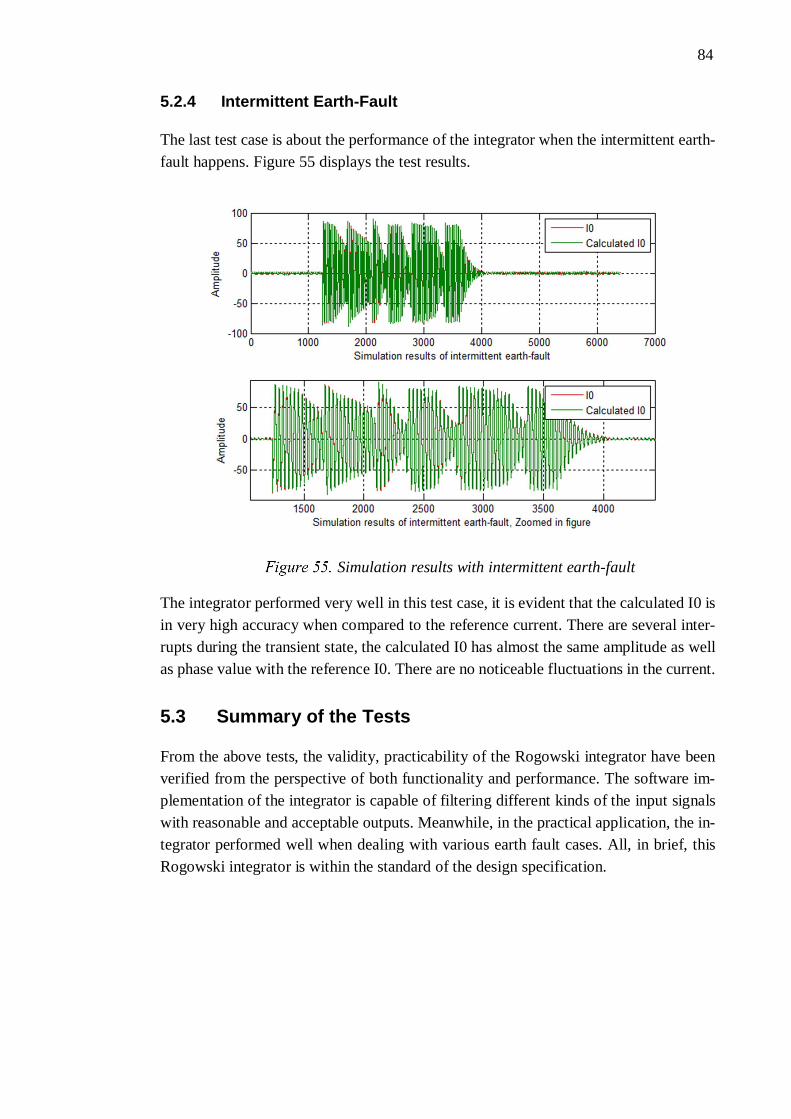
84
5.2.4 Intermittent Earth-Fault
The last test case is about the performance of the integrator when the intermittent earth-fault happens. Figure 55 displays the test results.
The integrator performed very well in this test case, it is evident that the calculated I0 isin very high accuracy when compared to the reference current. There are several inter-rupts during the transient state, the calculated I0 has almost the same amplitude as wellas phase value with the reference I0. There are no noticeable fluctuations in the current.
5.3 Summary of the Tests
From the above tests, the validity, practicability of the Rogowski integrator have beenverified from the perspective of both functionality and performance. The software im-plementation of the integrator is capable of filtering different kinds of the input signalswith reasonable and acceptable outputs. Meanwhile, in the practical application, the in-tegrator performed well when dealing with various earth fault cases. All, in brief, thisRogowski integrator is within the standard of the design specification.
Simulation results with intermittent earth-fault
85
6. CONCLUSIONS
6.1 Discussion
As an imperative part of the Rogowski sensor, the integrator plays a significant role inthe accuracy of the measured current. A lot of issues need to be considered when de-signing an integrator.
Choosing a good starting point filter for further improvements is necessary at the firststage. Several methods can be utilized during the design. In our design, the fundamentalprototype adopted is a trapezoidal integrator. Then we optimize the filter by increasingthe filter’s order with pole-zero placement. Pole-zero placement is a very efficient wayto increase or insert a particular notch/peak. The filter’s performance regularly turnsbetter after increasing its order. However the increase of the order comes along with theprice of more resource costs, a good designer should find a proper balance between theperformance and the costs.
Genetic Algorithm is used for the filter’s optimization. There are also other computa-tional algorithms for optimization, such as simulated annealing algorithm, differentialevolution algorithm, particle swarm algorithm, colony optimization algorithm, and Tabusearch algorithm, etc. [34]. The efficiency of Genetic Algorithm depends on how welldefined of the fitness function. The fitness function evaluates the filter’s performanceand gives corresponding fitness values. The evaluation standard refers a lot to the designspecification. Thus, a proper definition and analysis of the specification is veryimportant for the designer.
For a high order IIR filter, the general choice for the structure realization is the secondorder sections in cascade or parallel form. The decision also lies on the finite word-length effects if fixed point arithmetic is employed in the filter. The coefficients andintermediate variables’ accuracy will be degraded by the quantization effects, which willcause the filter’s performance deviation. Other finite word-length effects also affect theperformance of the filter. A good structure could effectively minify the effects to someextent.
There are two approaches to implementing the filter. One is software implementation,the other is hardware realization. Software approach in our case is realized by creatingthe MATLAB and C model of the integrator. By software implementation, the filtercould be simulated with targeted test benches. It is very efficient and valuable methodto exam the filter’s functionality before implementing it in the hardware. When the soft-ware implementation is verified, hardware implementation could be carried out if it isnecessary. In our case, RTL model is derived from the C model by translating it with

86
VHDL. Afterward, the integrator is implemented on FPGA board for practical fieldtests.
Based on the testing results, the performance of design integrator is very good whenreferring to the design specification. The basic magnitude and phase response of thecalculated I0 are of very high accuracy. Its ability of dealing with different earth faultsis also very good.
6.2 Challenge
There is always improvement remaining to be done. For this integrator, what could beconsidered to improve is the DC fluctuations caused by the noise in small currents. Onepossible solution is to increase the filter’s order, which may have a positive effect in thefrequency range around 0 Hz. The other method under consideration is to use new opti-mization method for searching even better filter coefficients.

87
REFERENCES
[1] Kojovic, Ljubomir. "Rogowski coils suit relay protection and measurement [ofpower systems]." Computer Applications in Power, IEEE 10.3 (1997): 47-52.
[2] Ward, David A., and J. La T. Exon. "Using Rogowski coils for transient currentmeasurements." Engineering Science & Education Journal 2.3 (1993): 105-113.
[3] Luo, Pandian, Hong-bin Li, and Zhen-Hua Li. "Two high accuracy digital inte-grators for Rogowski current transducers." Review of Scientific Instruments 85.1(2014): 015102.
[4] Zhang, Gang, et al. "A new electro-optic hybrid current-sensing scheme for cur-rent measurement at high voltage." Review of scientific instruments 70.9 (1999):3755-3758.
[5] Tong, Yue, and Bin Hong Li. "An accurate continuous calibration system forhigh voltage current transformer." Review of Scientific Instruments 82.2 (2011):025107.
[6] Becherini, G., et al. "Critical parameters for mutual inductance betweenRogowski coil and primary conductor." Instrumentation and Measurement Tech-nology Conference, 2009. I2MTC'09. IEEE. IEEE, 2009.
[7] Ljubomir Kojovic, Martin Bishop. Rogowski Coil Designs. Available:https://www.pacw.org/issue/autumn_2007_issue/protec-tion_rogowski/rogowski_coil_designs/complete_article/1.html
[8] Mitra S K, Kuo Y. Digital signal processing: a computer-based approach [M].New York: McGraw-Hill, 2006.
[9] IEEE Standard C37.235-2007, IEEE Guide for the Application ofRogowski Coils Used for Protective Relaying Purposes.
[10] V. Skendzic, B. Hughes. Using Rogowski coils inside protective relays[C]//Pro-tective Relay Engineers, 2013 66th Annual Conference for. IEEE, 2013: 1-10.
[11] Ramboz, John D. "Machinable Rogowski coil, design and calibration."Instru-mentation and Measurement Technology Conference, 1995. IMTC/95. Proceed-ings. Integrating Intelligent Instrumentation and Control., IEEE. IEEE, 1995.

88
[12] Sensor Technology, Applications for medium voltage, ABB Medium VoltageProducts. Available: http://www05.abb.com/global/scot/scot229.nsf/veritydis-play/576c37ea10824a4bc1257b12002a396d/$file/NewAndInnovativeWay_arti-cle_757842_ENa.pdf
[13] Xin Z, Longhua M. Design for digital integrator of Rogowski coil based on pipe-line structure[C]//Power and Energy Engineering Conference (APPEEC), 2010Asia-Pacific. IEEE, 2010: 1-4.
[14] D'Antona, G., et al. "AC current-to-voltage transducer based on digital pro-cessing of Rogowski coils signal." Sensors for Industry Conference, 2002. 2ndISA/IEEE. IEEE, 2002.
[15] 高迎霞, et al. "基于 Rogowski 线圈的电流互感器信号处理中积分算法的研
究."电测与仪表 43.11 (2007): 1-5.
[16] Ifeachor E C, Jervis B W. Digital signal processing: a practical approach[M].Pearson Education, 2002. P318-33, p455-62, 509-30,
[17] Hatem Bchir. Simultaneous Amplitude and Phase Optimization of IIR Filters.Master Thesis of Tampere University of Technology, 2009
[18] Hwang, Kai. Computer arithmetic: principles, architecture and design. JohnWiley & Sons, Inc., 1979.
[19] Cofer, R. C., and Ben Harding. "Fixed-Point DSP Algorithm Implementa-tion."EE Times-Ind
[20] Juha Yli Kaakinen. Optimization of Recursive Digital Filters for Practical Imple-mentations. Master Thesis of Tampere University of Technology, 2009
[21] Hussain, Zahir M., Amin Z. Sadik, and Peter O’Shea. Digital signal processing:an introduction with MATLAB and applications. Springer Science & BusinessMedia, 2011.
[22] Goldenberg, L. M., B. D. Matiushkin, and M. N. Poliak. "Digital signal pro-cessing: Handbook." Moscow Izdatel Radio Sviaz 1 (1985).
[23] Direct-Form I. Available: https://ccrma.stanford.edu/~jos/fp/Direct_Form_I.html
[24] Levi, E. C. "Complex-Curve Fitting." IRE Transactions on Automatic Control.Vol. AC-4, 1959, pp. 37–44.
89
[25] Dennis, J. E., Jr., and R. B. Schnabel. Numerical Methods for UnconstrainedOptimization and Nonlinear Equations. Englewood Cliffs, NJ: Prentice-Hall,1983.
[26] invfreqz - MathWorks - MATLAB and Simulink for Technical ...(n.d.). Availa-ble: http://www.mathworks.com/help/signal/ref/invfreqz.html
[27] Al-Alaoui M A. Class of digital integrators and differentiators [J]. IET SignalProcessing, 2011, 5(2): 251-260.
[28] Le Bihan, J. "Novel class of digital integrators and differentiators."ElectronicsLetters 29.11 (1993): 971-973.
[29] Hoffman, Joe D., and Steven Frankel. Numerical methods for engineers and sci-entists. CRC press, 2001.
[30] Al-Alaoui, Mohamad Adnan. "A class of second-order integrators and low-passdifferentiators." Circuits and Systems I: Fundamental Theory and Applications,IEEE Transactions on 42.4 (1995): 220-223.
[31] Ngo, Nam Quoc. "A new approach for the design of wideband digital integratorand differentiator." Circuits and Systems II: Express Briefs, IEEE Transactionson 53.9 (2006): 936-940.
[32] Thakur, Gaurav Kumar, Ankur Gupta, and D. Upadhyay. "Optimization Algo-rithm Approach for Error Minimization of Digital Integrators and Differentia-tors." ARTCom. 2009.
[33] Tseng, Chien-Cheng, and Su-Ling Lee. "Design of digital integrator using inter-laced sampling method and Simpson integration rule." Communications and In-formation Technologies (ISCIT), 2012 International Symposium on. IEEE, 2012.
[34] Tseng, C-C. "Digital integrator design using Simpson rule and fractional delayfilter." IEE Proceedings-Vision, Image and Signal Processing 153.1 (2006): 79-86.
[35] Al-Alaoui, Mohamad Adnan. "Class of digital integrators and differentia-tors."IET Signal Processing 5.2 (2011): 251-260.
[36] Tseng, Chien-Cheng, and Su-Ling Lee. "Digital IIR integrator design usingRichardson extrapolation and fractional delay." Circuits and Systems I: RegularPapers, IEEE Transactions on 55.8 (2008): 2300-2309.
[37] Jain, Madhu, Maneesha Gupta, and Nitin Jain. "Linear phase second order recur-sive digital integrators and differentiators." Radioengineering 21.2 (2012).

90
[38] Goldberg, David E., and John H. Holland. "Genetic algorithms and machinelearning." Machine learning 3.2 (1988): 95-99.
[39] Karaboga, Nurhan, and Bahadir Cetinkaya. "Design of minimum phase digitalIIR filters by using genetic algorithm." Proceedings of the 6th Nordic signalProcessing Symposium-NORSIG. Vol. 2004. 2004.
[40] Houck, Christopher R., Jeff Joines, and Michael G. Kay. "A genetic algorithmfor function optimization: a Matlab implementation." NCSU-IE TR95.09 (1995).
[41] Tang, Kit-Sang, et al. "Genetic algorithms and their applications." Signal Pro-cessing Magazine, IEEE 13.6 (1996): 22-37.
[42] Holland, John H. Adaptation in natural and artificial systems: an introductoryanalysis with applications to biology, control, and artificial intelligence. U Mich-igan Press, 1975.
[43] Joines, Jeffrey A., and Christopher R. Houck. "On the use of non-stationary pen-alty functions to solve nonlinear constrained optimization problems withGA's." Evolutionary Computation, 1994. IEEE World Congress on Computa-tional Intelligence., Proceedings of the First IEEE Conference on. IEEE, 1994.
[44] Gen, Mitsuo, and Runwei Cheng. Genetic algorithms and engineering optimiza-tion. Vol. 7. John Wiley & Sons, 2000.
[45] Galvanic Isolation, Available: http://en.wikipedia.org/wiki/Galvanic_isolation
[46] GNU MP Manual, Available: https://gmplib.org/manual/
[47] Newton–Cotes quadrature formula. Encyclopedia of Mathematics. Available:http://www.encyclopediaofmath.org/index.php?title=New-ton%E2%80%93Cotes_quadrature_formula&oldid=22841

91
APPENDIX: MATLAB CODES
1
2
3
4
5
6
b=[1 1]
a=[2 -2]
[z,p,k]=tf2zp(b,a)
if abs(p)>=1
p=0.9995*(real(p)/abs(p)+1i*imag(p)/abs(p));
end
Program 1. Example code for Trapezoidal Digital Integrator
1
2
3
4
5
6
b=[1 4 1]
a=[3 0 -3]
[z,p,k]=tf2zp(b,a)
if abs(p)>=1
p=0.9995*(real(p)/abs(p)+1i*imag(p)/abs(p))
end
Program 2. Example code for Simpson Digital Integrator
1
2
3
4
5
6
7
b=[0 1]
a=[1 -1]
[z,p,k]=tf2zp(b,a)
if abs(p)>=1
p=0.9995*(real(p)/abs(p)+1i*imag(p)/abs(p));
end
[b,a]=zp2tf(z,p,k)
Program 3. Example code for Rectangular Digital Integrator

92
1
2
3
4
5
6
7
8
9
10
11
12
13
14
15
16
17
18
b2=[1 1]
a2=[2 -2]
[z2,p2,k2]=tf2zp(b2,a2)
if abs(p2)>=1
p2=0.9995*(real(p2)/abs(p2)+1i*imag(p2)/abs(p2));
end
[b2,a2]=zp2tf(z2,p2,k2)
notchHz=0.5;%Hz
width=10;%Hz
notchAngle=360*notchHz/9600;
z2=[z2 cos(notchAngle*pi/180)+1i*sin(notchAngle*pi/180)];
z2= [z2 conj(z2(2))];
r=1-(width/9600)*pi;
p2=[p2 r*cos(notchAngle*pi/180)+1i*r*sin(notchAngle*pi/180)];
p2=[p2 conj(p2(2))];
x1=29.159320336410961
[b2,a2]=zp2tf(z2',p2',k2/x1)
fvtool(b2,a2)
Program 4. An example of higher order trapezoidal integrator
1
2
3
4
5
6
7
Fs=9600;
w = [0 pi*25/4800 pi*50/4800 pi*100/4800 pi*1600/4800 pi*4800/4800
mag = [0 2 1 0.5 0.03125 0.01041666 ]; %magnitudes
phase = [0/180*pi - 87/180*pi - 89.75/180*pi - 89.80/180*pi –
89.9/180*pi- 89.95/180*pi ]; % phases
wt = [1 1 10 10 10 10 ];
[b,a] = invfreqz(mag.*exp(1i*phase),w,3,3,wt,1000,0.01,'trace');
[zeroes, poles, k] = tf2zpk(b, a);
Program 5. Integrator design with direct design method
1
2
3
4
5
notchHz=0;
width=5;
notchAngle=360*notchHz/9600;
r=1-(width/9600)*pi;
z=[z cos(notchAngle*pi/180)+1i*sin(notchAngle*pi/180)];

93
6
7
8
z=[z conj(z(2))];
p=[p r*cos(notchAngle*pi/180)+1i*r*sin(notchAngle*pi/180)];
p=[p conj(p(2))];
result
z = [-1 1 1]
p = [0.999500000000000 0.998363753826255 0.998363753826255]
k = 0.016361741209689
Program 6. Example code for generating a 3rd order filter by pole zero place-ment
1
2
3
4
5
6
7
8
9
10
11
12
13
14
15
16
17
18
19
20
21
22
23
for j=1:N
notchHz=rand;%Hz
width=10*rand;% 0-20Hz
notchAngle=360*notchHz/9600;
r=1-(width/9600)*pi;
if j==1
zn(j) = -1 + 0.01*rand;
zn(j+1) = 0.99 + 0.01*rand;
elseif j==N
zn(j) = 0.99 + 0.1*rand;
end
if j==N
pn(j) = 0.99 + 0.01*rand;
else
pn(j)=(r*cos(notchAngle*pi/180)+1i*r*sin(notchAn
gle*pi/180));
notchHz=rand;%Hz
width=10*rand;% 0-20Hz
notchAngle=360*notchHz/9600;
r=1-(width/9600)*pi;
pn(j+1)=(r*cos(notchAngle*pi/180)-1i*r*sin(notchAn
gle*pi/180));
end
kn = 0.0162+0.0001*rand ;
end
Program 7. Example code for generating 3rd order filter of GA optimization
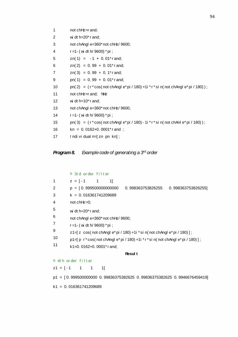
94
1
2
3
4
5
6
7
9
10
11
12
13
14
15
16
17
notchHz=rand;
width=20*rand;
notchAngle=360*notchHz/9600;
r=1-(width/9600)*pi;
zn(1) = -1 + 0.01*rand;
zn(2) = 0.99 + 0.01*rand;
zn(3) = 0.99 + 0.1*rand;
pn(1) = 0.99 + 0.01*rand;
pn(2) = (r*cos(notchAngle*pi/180)+1i*r*sin(notchAngle*pi/180));
notchHz=rand; %Hz
width=10*rand;
notchAngle=360*notchHz/9600;
r=1-(width/9600)*pi;
pn(3) = (r*cos(notchAngle*pi/180)-1i*r*sin(notchAnle*pi/180));
kn = 0.0162+0.0001*rand ;
Individualn=[zn pn kn];
Program 8. Example code of generating a 3rd order
1
2
3
4
5
6
7
9
10
11
% 3rd order filter
z = [-1 1 1]
p = [0.999500000000000 0.998363753826255 0.998363753826255]
k = 0.016361741209689
notchHz=0;
width=20*rand;
notchAngle=360*notchHz/9600;
r=1-(width/9600)*pi;
z1=[z cos(notchAngle*pi/180)+1i*sin(notchAngle*pi/180)];
p1=[p r*cos(notchAngle*pi/180)+1i*r*sin(notchAngle*pi/180)];
k1=0.0162+0.0001*rand;
Result
% 4th order filter
z1 = [-1 1 1 1]
p1 = [0.999500000000 0.99836375382625 0.99836375382625 0.9946676459419]
k1 = 0.016361741209689

95
Program 9. Example code for generating a 4th order integrator by adding anotch exactly at 0 Hz
1
2
3
4
5
6
7
9
10
11
12
13
14
15
16
17
18
19
20
21
22
23
notchHz=rand; %put zero in the range [0,5]Hz
width=5*rand; %width of notch 0-5Hz
notchAngle=360*notchHz/9600;
r=1-(width/9600)*pi;
zn(1) = -1 + 0.01*rand;
zn(2) = 0.99 + 0.01*rand;
zn(3) = 0.99 + 0.01*rand;
zn(4)= cos(notchAngle*pi/180)+1i*sin(notchAngle*pi/180);
pn(1) = (0.99 + 0.01*rand);
pn(4) = r*cos(notchAngle*pi/180)+1i*r*sin(notchAngle*pi/180);
notchHz=10*rand; %put zero in the range [0,10]Hz
width=20*rand; %width of notch 0-20Hz
notchAngle=360*notchHz/9600;
r=1-(width/9600)*pi;
pn(2)=r*cos(notchAngle*pi/180)+1i*r*sin(notchAngle*pi/180);
notchHz=10*rand;
width=20*rand;
notchAngle=360*notchHz/9600;
r=1-(width/9600)*pi;
pn(3)=r*cos(notchAngle*pi/180)-1i*r*sin(notchAngle*pi/180);
kn=0.0162+0.0001*rand;
Individualn=[zn pn kn];
Program 10. Example code for creating new filters for 4th order filter optimization