mfca’08 - · pdf filemfca’08 september 6 th, 2008, ... sarang joshi (sci,...
TRANSCRIPT
MFCA’08
September 6th, 2008, Kimmel Center, New York, USA.
http://www.inria.fr/sophia/asclepios/events/MFCA08
Editors:
Xavier Pennec (Asclepios, INRIA Sophia-Antipolis, France) Sarang Joshi (SCI, University of Utah, USA)
Mathematical Foundations of
Computational Anatomy
Geometrical and Statistical Methods for Biological Shape Variability Modeling

Preface
The goal of computational anatomy is to analyze and to statistically model theanatomy of organs in different subjects. Computational anatomic methods aregenerally based on the extraction of anatomical features or manifolds which arethen statistically analyzed, often through a non-linear registration. There arenowadays a growing number of methods that can faithfully deal with the un-derlying biomechanical behavior of intra-subject deformations. However, it ismore difficult to relate the anatomies of different subjects. In the absence ofany justified physical model, diffeomorphisms provide a general mathematicalframework that enforce topological consistency. Working with such infinite di-mensional space raises some deep computational and mathematical problems, inparticular for doing statistics. Likewise, modeling the variability of surfaces leadsto rely on shape spaces that are much more complex than for curves. To copewith these, different methodological and computational frameworks have beenproposed (e.g. smooth left-invariant metrics, focus on well-behaved subspaces ofdiffeomorphisms, modeling surfaces using courants, etc.)
The goal of the Mathematical Foundations of Computational Anatomy(MFCA) workshop is to foster the interactions between the mathematicalcommunity around shapes and the MICCAI community around computationalanatomy applications. It targets more particularly researchers investigating thecombination of statistical and geometrical aspects in the modeling of the vari-ability of biological shapes. The workshop aims at being a forum for the ex-change of the theoretical ideas and a source of inspiration for new method-ological developments in computational anatomy. A special emphasis is puton theoretical developments, applications and results being welcomed as illus-trations. Following the very successful first edition of this workshop in 2006(see http://www.inria.fr/sophia/asclepios/events/MFCA06/), the second edi-tion was held in New-York on September 6, in conjunction with MICCAI 2008.
Contributions were solicited in Riemannian and group theoretical methods,Geometric measurements of the anatomy, Advanced statistics on deformationsand shapes, Metrics for computational anatomy, Statistics of surfaces. 34 sub-missions were received, among which 9 were accepted to MICCAI and had to bewithdrawn from the workshop. Each of the remaining 25 paper was reviewed bythree members of the program committee. To guaranty a high level program, 16papers only were selected.
August 2008 Xavier PennecGeneral Chair
MFCA’08

Organization
Workshop Chairs
Xavier Pennec (INRIA Sophia-Antipolis, France)Sarang Joshi (SCI, University of Utah, USA)
Program Committee
Rachid Deriche (INRIA, France)Ian L. Dryden (University of Nottingham, UK)Tom Fletcher (University of Utah, USA)James Gee (Univ. of Pennsylvania, USA)Guido Gerig (University of Utah, USA)Polina Golland (CSAIL, MIT, USA)Stephen Marsland (Massey University, New-Zeeland)Michael I. Miller (John Hopkins University, USA)Mads Nielsen (IT University of Copenhagen, Denmark)Salvador Olmos (University of Saragossa, Spain)Bruno Pelletier (University Montpellier, France)Jerry Prince (Johns Hopkins University, USA)Anand Rangarajan (University of Florida, USA)Daniel Rueckert (Imperial College London, UK)Guillermo Sapiro (University of Minnesota, USA)Martin Styner (UNC Chapel Hill, USA)Anuj Srivastava (Florida State University, USA)Paul Thompson (University of California Los-Angeles, USA)Alain Trouve (ENS-Cachan, France)Carole Twinning (University of Manchester, UK)William M. Wells III (CSAIL, MIT, and B&W Hospital, Boston, USA)
Table of Contents
Registration
Unbiased Volumetric Registration via Nonlinear Elastic Regularization . . 1Igor Yanovsky, Carole Le Guyader, Alex Leow, Arthur Toga, PaulThompson, and Luminita Vese
A new algorithm for the computation of the group logarithm ofdiffeomorphisms . . . . . . . . . . . . . . . . . . . . . . . . . . . . . . . . . . . . . . . . . . . . . . . . . . 13
Matias Bossa and Salvador Olmos
Comparing algorithms for diffeomorphic registration: StationaryLDDMM and Diffeomorphic Demons . . . . . . . . . . . . . . . . . . . . . . . . . . . . . . . . 24
Monica Hernandez, Salvador Olmos, and Xavier Pennec
Morphometry
Brain Mapping with the Ricci Flow Conformal Parameterization andMultivariate Statistics on Deformation Tensors . . . . . . . . . . . . . . . . . . . . . . . 36
Yalin Wang, Xiaotian Yin, Jie Zhang, Xianfeng Gu, Tony F.Chan, Paul M. Thompson, and Shing-Tung Yau
Multi-Atlas Tensor-Based Morphometry and its Application to aGenetic Study of 92 Twins . . . . . . . . . . . . . . . . . . . . . . . . . . . . . . . . . . . . . . . . . 48
Natasha Lepore, Caroline Brun, Yi-Yu Chou, Agatha D. Lee,Marina Barysheva, Greig I. de Zubicaray, Matthew Meredith, KatieL. McMahon, Margaret J. Wright, Arthur W. Toga, and Paul M.Thompson
Shape Registration with Spherical Cross Correlation . . . . . . . . . . . . . . . . . . . 56Boris Gutman, Yalin Wang, Tony Chan, Paul M. Thompson, andArthur W. Toga
Building Atlases
A Forward Model to Build Unbiased Atlases from Curves and Surfaces . . 68Stanley Durrleman, Xavier Pennec, Alain Trouve, and NicholasAyache

IV
MAP Estimation of Statistical Deformable Templates Via NonlinearMixed Effects Models : Deterministic and Stochastic Approaches . . . . . . . . 80
Stephanie Allassonniere, Estelle Kuhn, and Alain Trouve
Semiparametric estimation of rigid transformations on compact Lie groups 92Jeremie Bigot, Jean-Michel Loubes and Myriam Vimond
Shapes and Surfaces
Geodesic Shape Spaces of Surfaces of Genus Zero . . . . . . . . . . . . . . . . . . . . . 105Xiuwen Liu, Washington Mio, Yonggang Shi, and Ivo Dinov
Characterization of Anatomical Shape Based on Random Walk HittingTimes . . . . . . . . . . . . . . . . . . . . . . . . . . . . . . . . . . . . . . . . . . . . . . . . . . . . . . . . . . . 117
Grace Vesom, Nathan D. Cahill, Lena Gorelick, and J. Alison Noble
Tiling Manifolds with Orthonormal Basis . . . . . . . . . . . . . . . . . . . . . . . . . . . . 128Moo K. Chung, Anqi Qiu, Brendon M. Nacewicz, Seth Pollak,Richard J. Davidson
Statistics on Manifolds and Shapes
Diffusion Tensor Imaging and Deconvolution on Spaces of PositiveDefinite Symmetric Matrices . . . . . . . . . . . . . . . . . . . . . . . . . . . . . . . . . . . . . . . 140
Peter T. Kim and Donald St. P. Richards
Tubular Surface Evolution for Segmentation of the Cingulum BundleFrom DW-MRI . . . . . . . . . . . . . . . . . . . . . . . . . . . . . . . . . . . . . . . . . . . . . . . . . . . 150
Vandana Mohan, Ganesh Sundaramoorthi, John Melonakos, MarcNiethammer, Marek Kubicki, and Allen Tannenbaum
Modeling the Remaining Flexibility of Partially Fixed Statistical ShapeModels . . . . . . . . . . . . . . . . . . . . . . . . . . . . . . . . . . . . . . . . . . . . . . . . . . . . . . . . . . 160
Thomas Albrecht, Reinhard Knothe, and Thomas Vetter
A Hypothesis Testing Framework for High-Dimensional Shape Models . . . 170Joshua Cates, P. Thomas Fletcher, Ross Whitaker
Author Index . . . . . . . . . . . . . . . . . . . . . . . . . . . . . . . . . . . . . . . . . . . . . . . . 182

Unbiased Volumetric Registration via Nonlinear ElasticRegularization
Igor Yanovsky1, Carole Le Guyader2, Alex Leow3, Arthur Toga3,Paul Thompson3, and Luminita Vese1
1 Department of Mathematics, University of California, Los Angeles, USA,2 Institute of Mathematical Research of Rennes, France,
3 Laboratory of Neuro Imaging, UCLA School of Medicine, USA. ?
Abstract. In this paper, we propose a new large-deformation nonlinear imageregistration model in three dimensions, based on nonlinear elastic regularizationand unbiased registration. Both the nonlinear elastic and the unbiased functionalsare simplified introducing, in the modeling, a second unknown that mimics theJacobian matrix of the displacement vector field, reducing the minimization to in-volve linear differential equations. In contrast to recently proposed unbiased fluidregistration method, the new model is written in a unified variational form andis minimized using gradient descent on the corresponding Euler-Lagrange equa-tions. As a result, the new unbiased nonlinear elasticity model is computationallymore efficient and easier to implement than the unbiased fluid registration. Themodel was tested using three-dimensional serial MRI images and shown to havesome advantages for computational neuroimaging.
1 Introduction
Given two images, the source and target, the goal of image registration is to find anoptimal diffeomorphic spatial transformation such that the deformed source image isaligned with the target image. In the case of non-parametric registration methods (theclass of methods we are interested in), the problem can be phrased as a functionalminimization problem whose unknown is the displacement vector field u. Usually, thedevised functional consists of a distance measure (intensity-based, correlation-based,mutual-information based [1] or metric-structure-comparison based [2]) and a regular-izer that guarantees smoothness of the displacement vector field. Several regularizershave been investigated (see Part II of [1] for a review). Generally, physical argumentsmotivate the selection of the regularizer. Among those currently used is the linear elas-ticity smoother first introduced by Broit [3]. The objects to be registered are consideredto be observations of the same elastic body at two different times, before and afterbeing subjected to a deformation as mentioned in [1]. The smoother, in this case, isthe linearized elastic potential of the displacement vector field. However, this model isunsuitable for problems involving large-magnitude deformations.
? This work was funded by the National Institutes of Health through the NIH Roadmap forMedical Research, Grant U54 RR021813 entitled Center for Computational Biology (CCB).
2 I. Yanovsky et al.
In [4], Christensen et al. proposed a viscous fluid model to overcome this issue.The deforming image is considered to be embedded in viscous fluid whose motion isgoverned by Navier-Stokes equations for conservation of momentum:
µ4v(x, t) + (ν + µ)∇(∇ · v(x, t)) = f(x, u(x, t)), (1)v(x, t) = ut(x, t) +∇u(x, t) · v(x, t). (2)
Here, equation (2), defining material derivative of u, nonlinearly relates the velocity anddisplacement vector fields.
One drawback of this method is the computational cost. Numerically, the image-derived force field f(x, u(x, t)) is first computed at time t. Fixing the force field f, lin-ear equation (1) is solved for v(x, t) numerically using the successive over-relaxation(SOR) scheme. Then, an explicit Euler scheme is used to advance u in time. Recentworks [5–7] applied Riemannian nonlinear elasticity priors to deformation velocityfields. These alternating frameworks, however, are time-consuming, which motivatesthe search for faster implementations (see for instance [8] or [9] in which the instanta-neous velocity v is obtained by convolving f with a Gaussian kernel).
In this paper, which is inspired from related works on segmentation [10] and ontwo-dimensional registration [11], we propose an alternative approach to fluid registra-tion. The new model is derived from a variational problem which is not in the form ofa two-step algorithm and which can also produce large-magnitude deformations. Forthat purpose, a nonlinear elasticity smoother is introduced in three dimensions. As willbe seen later, the computation of the Euler-Lagrange equations in this case is cumber-some. We circumvent this issue by introducing a second unknown, a matrix variableV , which approximates the Jacobian matrix of u. The nonlinear elastic regularizer isnow applied to V , removing the nonlinearity in the derivatives of the unknown u in theEuler-Lagrange equations. The Euler-Lagrange equations are straightforwardly derivedand a gradient descent method is used.
Also, allowing large deformations to occur may yield non-diffeomorphic defor-mation mappings. In [4], Christensen et al. proposed a regridding technique that re-samples the deforming image and re-initializes the process once the value of the de-formation Jacobian drops below a certain threshold. In [12], Haber and Modersitzkiintroduced an elastic registration model subjected to volume-preserving constraints.To ensure that the transformation g(x) = x − u(x) is volume-preserving (that is, forany domain Ω,
∫Ω
dx =∫
g(Ω)dx), they proposed the following pointwise constraint:
det(I −Du(x))−1 = 0. Pursuing in the same direction in [13], the authors introduceda minimization problem under inequality constraints on the Jacobian.
Here we use an information-theoretic approach previously introduced in [14]. In[14], the authors considered a smooth deformation g that maps domain Ω bijectivelyonto itself. Consequently, g and g−1 are bijective and globally volume-preserving. Prob-ability density functions can thus be associated with the deformation g and its inverseg−1. The authors then proposed to quantify the magnitude of the deformation by meansof the symmetric Kullback-Leibler distance between the probability density functionsassociated with the deformation and the identity mapping. This distance, when rewrit-ten using skew-symmetry properties, is viewed as a cost function and is combined withthe viscous fluid model for registration, which leads to an unbiased fluid registration

Unbiased Volumetric Registration via Nonlinear Elastic Regularization 3
model. Unlike the unbiased fluid registration model, the unbiased nonlinear elasticitymethod, introduced here, allows the functional to be written “in closed form”. The newmodel also does not require expensive Navier-Stokes solver (or its approximation) ateach step as previously mentioned.
2 Method
Let Ω be an open and bounded domain in R3. Without loss of generality, we assumethat the volume of Ω is 1, i.e. |Ω| = 1. Let I1, I2 : Ω → R be the two images to beregistered. We seek the transformation g : Ω → Ω that maps the source image I2 intocorrespondence with the target image I1. In this paper, we will restrict this mapping tobe differentiable, one-to-one, and onto. We denote the Jacobian matrix of a deformationg to be Dg, with Jacobian denoted by |Dg(x)| = det(Dg(x)) (thus we will use thenotation |V | := det(V ) for any 3 × 3 matrix V ). The displacement field u(x) fromthe position x in the deformed image I2 g(x) back to I2(x) is defined in terms of thedeformation g(x) by the expression g(x) = x − u(x) at every point x ∈ Ω. Thus, weconsider the problems of finding g and u as equivalent.
In general, nonlinear image registration models may be formulated in a variationalframework. The minimization problems often define the energy functional E as a linearcombination of image matching term F and the regularizing term R: infuE(u) =F (u) + λ0R(u). Here, λ0 > 0 is a weighting parameter.
2.1 Registration metrics
In this paper, the matching functional F takes the form of the L2 norm (the sum ofsquared intensity differences), F = FL2 , and the mutual information, F = FMI .L2-norm: The L2-norm matching functional is suitable when the images have beenacquired through similar sensors (with additive Gaussian noise) and thus are expectedto present the same intensity range and distribution. The L2 distance between the de-formed image I2 g(x) = I2(x− u(x)) and target image I1(x) is defined as
FL2(u) =12
∫Ω
(I2(x− u(x))− I1(x)
)2dx. (3)
Mutual Information: Mutual information can be used to align images of differentmodalities, without requiring knowledge of the relationship of the two registered im-ages [15, 16]. Here, the intensity distributions estimated from I1(x) and I2(x − u(x))are denoted by pI1 and pI2
u , respectively, and an estimate of their joint intensity distri-bution by pI1,I2
u . We let i1 = I1(x), i2 = I2(x − u(x)) denote intensity values at pointx ∈ Ω. Given the displacement field u, the mutual information computed from I1 and I2
is provided by MII1,I2u =
∫R2 pI1,I2
u (i1, i2) log[pI1,I2u (i1, i2)/(pI1(i1)pI2
u (i2))] di1di2.We seek to maximize the mutual information between I2(x−u(x)) and I1(x), or equiv-alently, minimize the negative of MII1,I2
u :
FMI(I1, I2, u) = −MII1,I2u . (4)

4 I. Yanovsky et al.
2.2 Nonlinear Elastic Regularization
The theory of elasticity is based on the notion of strain. Strain is defined as the amountof deformation an object experiences compared to its original size and shape. In threespatial dimensions, the strain tensor, E = [εij ] ∈ R3×3, 1 ≤ i, j ≤ 3, is a symmetrictensor used to quantify the strain of an object undergoing a deformation. The nonlinearstrain is defined as εij(u) = 1
2
(∂jui + ∂iuj +
∑3k=1 ∂iuk∂juk
), with the nonlinear
strain tensor matrix given by
E(u) =12(Dut + Du + DutDu
). (5)
Stored energy (Saint Venant-Kirchhoff material) is defined as
W (E) =ν
2(trace(E))2 + µtrace(E2),
where ν and µ are Lame elastic material constants. The regularization for nonlinearelasticity becomes
RE(u) =∫
Ω
W (E(u))dx.
The regularization term RE(u) can be minimized with respect to u. However, since theregularization term is written in terms of partial derivatives of components of u, theEuler-Lagrange equations become complicated and are computationally expensive tominimize. Instead, following earlier theoretical work [17], we minimize an approximatefunctional by introducing the matrix variable
V ≈ Du (6)
and thus consider a new form of nonlinear elasticity regularization functional
RE(u, V ) =∫
Ω
W (V ) dx +β
2
∫Ω
||V −Du||2F dx, (7)
where V =12(V t + V + V tV
), β is a positive constant, and || · ||F denotes the Frobe-
nius norm. For β large enough, RE(u) is well approximated by RE(u, V ). In the limitas β → +∞, we obtain Du ≈ V in the L2- topology.
The idea of duplication of variables was also used in previous work [18] by Cachieret al. but for a different problem. In their case, the registration energy depends on twovariables that are both vector fields. The first vector field C is a set of correspondencesbetween points based on intensity similarity, while the second, denoted by T, is asmooth vector field constrained by the regularization energy and attracted by the setof correspondences C.
Unbiased Volumetric Registration via Nonlinear Elastic Regularization 5
2.3 Unbiased Registration Constraint
In [14], the authors proposed an unbiased fluid image registration approach. Contraryto classical methods for which the term unbiased is used in the sense of symmetricregistration, in [14], unbiased means that the Jacobian determinants of the deformationsrecovered between a pair of images follow a log-normal distribution, with zero meanafter log-transformation. The authors argued that this distribution is beneficial whenrecovering change in regions of homogeneous intensity, and in ensuring symmetricalresults when the order of two images being registered is switched. As derived in [14]using information theory, the unbiased regularization term is given as
RUB(u) =∫
Ω
(|D(x− u(x))| − 1
)log |D(x− u(x))|dx. (8)
It is important to note that RUB generates inverse-consistent deformation maps. Theinverse-consistent property of the unbiased technique was shown in a validation study ofthe unbiased fluid registration methods [19]. Also, to see why minimizing equation (8)leads to unbiased deformation in the logarithmic space, we observe that the integrandis always non-negative, and only evaluates to zero when the deformation g is volume-preserving everywhere (|Dg| = 1 everywhere). Thus, by treating it as a cost, we recoverzero-change by minimizing this cost when we compare images differing only in noise.
Given equation (6), we have Dg = I −Du ≈ I − V , where I is the 3× 3 identitymatrix. Therefore, as in subsection 2.2, to simplify the discretization, we introduce
RUB(V ) =∫
Ω
(|I − V | − 1) log |I − V | dx. (9)
Recall that here |I − V | = det(I − V ).
2.4 Unbiased Nonlinear Elasticity Registration
The total energy functional employed in this work, is given as a linear combination ofthe similarity measure F (which is either FL2 from (3) or FMI from (4)), nonlinearelastic regularization RE in (7), and unbiased regularization RUB in (9):
E(u, V ) = F (u) + RE(u, V ) + λRUB(V ). (10)
The explicit weighting parameter is omitted in front of RE(u, V ), since this term isweighted by Lame constants ν and µ. We solve the Euler-Lagrange equations in uand V using the gradient descent method, parameterizing the descent direction by anartificial time t,
∂u∂t
= −∂Eu(u, V ) = −∂uF (u)− ∂uRE(u, V ), (11)
∂V
∂t= −∂EV (u, V ) = −∂V RE(u, V )− λ∂V RUB(V ), (12)
which gives systems of three and nine equations, respectively. Explicit expressions forthe gradients in these equations are given in Section 3.

6 I. Yanovsky et al.
Remark 1. The regularization on the deformation g proposed in this work can be ex-pressed in a general form R(g) =
∫Ω
R1(Dg)dx +∫
ΩR2(|Dg|)dx, with |Dg| :=
det(Dg). For the minimization, an auxiliary variable can also be introduced to simplifythe numerical calculations, removing the nonlinearity in the derivatives.
3 Implementation
3.1 The Energy Gradients
Computing the first variation of functional RE(u, V ), in equation (7), with respect to ugives the following components of gradient ∂uRE(u, V ):
∂ukRE(u, V ) = β
(∂1vk1 + ∂2vk2 + ∂3vk3 −4uk
), k = 1, 2, 3.
The first variation of RE(u, V ) with respect to V , with V = [vij ], gives ∂V RE(u, V ):
∂v11RE(u, V ) = β(v11 − ∂1u1) + νc1(1 + v11) + µ(c2(1 + v11) + c5v12 + c6v13
),
∂v12RE(u, V ) = β(v12 − ∂2u1) + νc1v12 + µ(c3v12 + c5(1 + v11) + c7v13
),
∂v13RE(u, V ) = β(v13 − ∂3u1) + νc1v13 + µ(c4v13 + c6(1 + v11) + c7v12
),
∂v21RE(u, V ) = β(v21 − ∂1u2) + νc1v21 + µ(c2v21 + c5(1 + v22) + c6v23
),
∂v22RE(u, V ) = β(v22 − ∂2u2) + νc1(1 + v22) + µ(c3(1 + v22) + c5v21 + c7v23
),
∂v23RE(u, V ) = β(v23 − ∂3u2) + νc1v23 + µ(c4v23 + c6v21 + c7(1 + v22)
),
∂v31RE(u, V ) = β(v31 − ∂1u3) + νc1v31 + µ(c2v31 + c5v32 + c6(1 + v33)
),
∂v32RE(u, V ) = β(v32 − ∂2u3) + νc1v32 + µ(c3v32 + c5v31 + c7(1 + v33)
),
∂v33RE(u, V ) = β(v33 − ∂3u3) + νc1(1 + v33) + µ(c4(1 + v33) + c6v31 + c7v32
),
where
c1 = v11 + v22 + v33 +12(v211 + v2
21 + v231 + v2
12 + v222 + v2
32 + v213 + v2
23 + v233
),
c2 = 2v11 + v211 + v2
21 + v231, c5 = v21 + v12 + v11v12 + v21v22 + v31v32,
c3 = 2v22 + v212 + v2
22 + v232, c6 = v31 + v13 + v11v13 + v21v23 + v31v33,
c4 = 2v33 + v213 + v2
23 + v233, c7 = v32 + v23 + v12v13 + v22v23 + v32v33.
We can compute the first variation of (9), obtaining ∂V RUB(V ). We first simplifythe notation, letting J = |I − V |. Also, denote L(J) = (J − 1) log J . Hence, L′(J) =

Unbiased Volumetric Registration via Nonlinear Elastic Regularization 7
dL(J)/dJ = 1 + log J − 1/J . Thus,
∂v11RUB(V ) = −((1− v22)(1− v33)− v32v23
)L′(J),
∂v12RUB(V ) = −(v23v31 + v21(1− v33)
)L′(J),
∂v13RUB(V ) = −(v21v32 + (1− v22)v31
)L′(J),
∂v21RUB(V ) = −(v32v13 + v12(1− v33)
)L′(J),
∂v22RUB(V ) = −((1− v11)(1− v33)− v13v31
)L′(J),
∂v23RUB(V ) = −(v12v31 + v32(1− v11)
)L′(J),
∂v31RUB(V ) = −(v12v23 + v13(1− v22)
)L′(J),
∂v32RUB(V ) = −(v21v13 + v23(1− v11)
)L′(J),
∂v33RUB(V ) = −((1− v11)(1− v22)− v12v21
)L′(J).
3.2 Algorithm
We are now ready to give the algorithm for the unbiased registration via nonlinear elas-tic regularization.
Algorithm 1 Unbiased Registration via Nonlinear Elastic Regularization1: Initialize t = 0, u(x, 0) = 0, and V (x, 0) = 0.2: Calculate V (x, t) using equation (12).
Steps 3-5 describe the procedure for solving equation (11).3: Calculate the perturbation of the displacement field R(x) = −∂Eu(u, V ).4: Time step 4t is calculated adaptively so that 4t · max(||R||2) = δu, where δu is the
maximal displacement allowed in one iteration. Results in this work are obtained with δu =0.1.
5: Advance equation (11), i.e. ∂u(x, t)/∂t = R(x), in time, with time step from step 4, solvingfor u(x, t).
6: If the cost functional in (10) decreases by sufficiently small amount compared to the previousiteration, then stop.
7: Let t := t + 4t and go to step 2.
4 Results and Discussion
We tested the proposed unbiased nonlinear elastic registration model and comparedthe results to those obtained with the unbiased fluid registration method [14], wherethe unbiased regularization constraint (8) was coupled with the L2 matching functional(3) and fluid regularization (1), (2). Here, both methods were coupled with the L2 andmutual information (MI) based similarity measures. In our experiments, we used a pairof serial MRI images (220 × 220 × 220) from the Alzheimer’s Disease NeuroimagingInitiative (ADNI). Since the images were acquired one year apart, from a subject with

8 I. Yanovsky et al.
Volume I1
Volume I2
Fig. 1. Serial MRI images from the ADNI follow-up dataset (images acquired one year apart) areshown. Volumes I1 (row 1) and I2 (row 2) are depicted as a brain volume (column 1) and fromsagittal (column 2), axial (column 3), and coronal (column 4) views. Nonrigid registration alignsvolume I2 into correspondence with volume I1.
Alzheimer’s disease, real anatomical changes are present, which allows methods to becompared in the presence of true biological changes.
In the tests performed using unbiased nonlinear elasticity coupled with L2 match-ing, values of β = 20000 in equation (7) and λ = 2000 in equation (10) were chosen.For MI matching, β = 80 and λ = 8 were used. The values of the Lame coefficientswere chosen to be equal, µ = ν, in all experiments. Bigger values of µ and ν allow formore smoothing. For unbiased fluid registration model, described in [14], λ = 500 waschosen for L2 matching, and λ = 5 for MI matching.
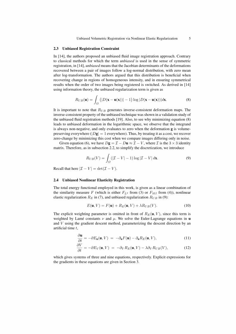
Figure 2 shows the images being registered along with the resulting Jacobian maps.Results generated using the fluid and nonlinear elasticity based unbiased models aresimilar, both suggesting a mild volume reduction in gray and white matter and ven-tricular enlargement that is observed in Alzheimer’s disease patients. The advantagesof the unbiased nonlinear elasticity model is its more locally plausible reproduction ofatrophic changes in the brain and its robustness to original misalignment of brain vol-umes, which is especially noticeable on the brain surface. The unbiased nonlinear elas-ticity model coupled with L2 matching generated very similar results to those obtainedwith the MI similarity measure, partly because difference images typically contain onlynoise after registration. Unbiased fluid registration method, however, is more effectivein modeling the regional neuroanatomical changes, showing more clearly which partsof the volume have undergone largest tissue changes, such as ventricular enlargementas shown in Figure 2.
Figure 3 shows deformed grids generated with unbiased fluid and unbiased nonlin-ear elastic registration models. Figure 4 shows the energy decrease per iteration for bothmodels.
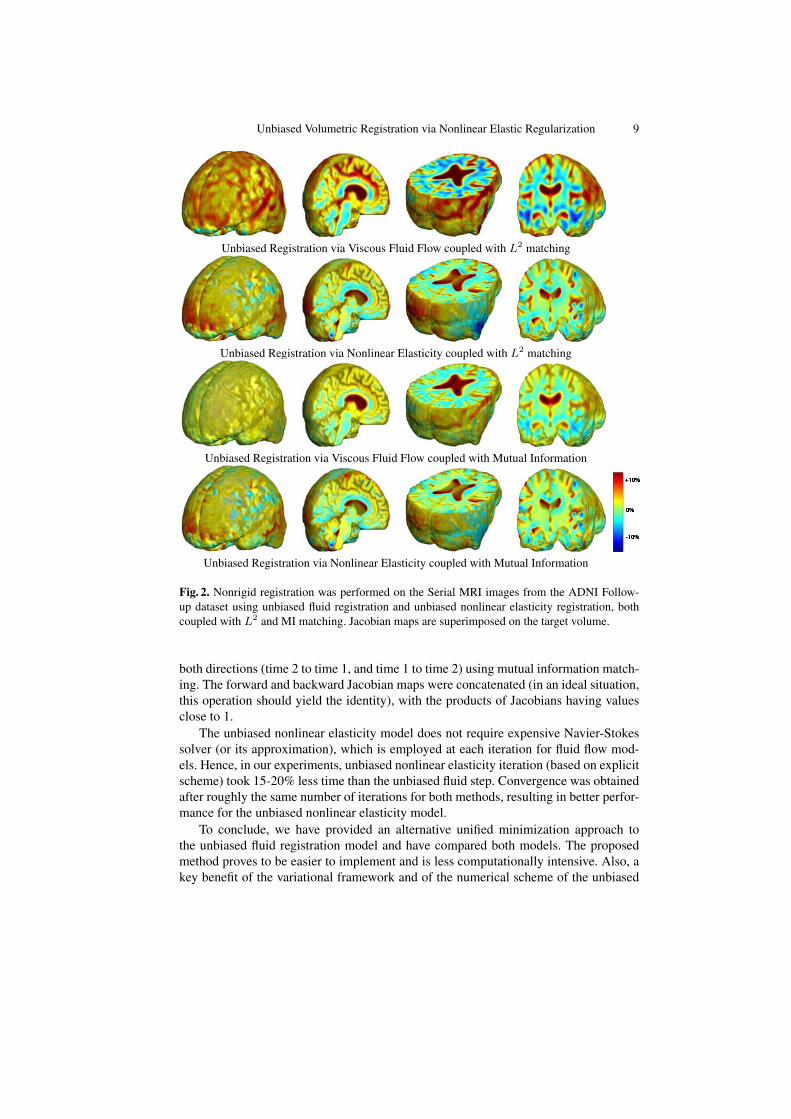
In Figure 5, we examined the inverse consistency of the mappings [20] generatedusing unbiased nonlinear elastic registration. Here, the deformation was computed in
Unbiased Volumetric Registration via Nonlinear Elastic Regularization 9
Unbiased Registration via Viscous Fluid Flow coupled with L2 matching
Unbiased Registration via Nonlinear Elasticity coupled with L2 matching
Unbiased Registration via Viscous Fluid Flow coupled with Mutual Information
Unbiased Registration via Nonlinear Elasticity coupled with Mutual Information
Fig. 2. Nonrigid registration was performed on the Serial MRI images from the ADNI Follow-up dataset using unbiased fluid registration and unbiased nonlinear elasticity registration, bothcoupled with L2 and MI matching. Jacobian maps are superimposed on the target volume.
both directions (time 2 to time 1, and time 1 to time 2) using mutual information match-ing. The forward and backward Jacobian maps were concatenated (in an ideal situation,this operation should yield the identity), with the products of Jacobians having valuesclose to 1.
The unbiased nonlinear elasticity model does not require expensive Navier-Stokessolver (or its approximation), which is employed at each iteration for fluid flow mod-els. Hence, in our experiments, unbiased nonlinear elasticity iteration (based on explicitscheme) took 15-20% less time than the unbiased fluid step. Convergence was obtainedafter roughly the same number of iterations for both methods, resulting in better perfor-mance for the unbiased nonlinear elasticity model.
To conclude, we have provided an alternative unified minimization approach tothe unbiased fluid registration model and have compared both models. The proposedmethod proves to be easier to implement and is less computationally intensive. Also, akey benefit of the variational framework and of the numerical scheme of the unbiased

10 I. Yanovsky et al.
Unbiased models with L2 matching Unbiased models with MI matchingFluid Nonl.Elasticity Fluid Nonl.Elasticity
Fig. 3. Results obtained using unbiased fluid registration and unbiased nonlinear elasticity regis-tration, both coupled with L2 and MI matching. The generated grids are superimposed on top of2D cross-sections of the 3D volumes (row 1) and are shown separately (row 2).
0 200 400 600 800 100020
40
60
80
100
Iteration number
Ene
rgy
Unbiased−Fluid L2
0 200 400 600 800 100020
40
60
80
100
Iteration number
Ene
rgy
Unbiased−NE L2
0 200 400 600 800 1000−1.6
−1.55
−1.5
−1.45
−1.4
−1.35
Iteration number
Ene
rgy
Unbiased−Fluid MI
0 200 400 600 800 1000−1.6
−1.55
−1.5
−1.45
−1.4
−1.35
Iteration number
Ene
rgy
Unbiased−NE MI
Unbiased models with L2 matching Unbiased models with MI matchingFluid Nonl.Elasticity Fluid Nonl.Elasticity
Fig. 4. Energy per iteration for the unbiased fluid registration and unbiased nonlinear elasticityregistration, both coupled with L2 and MI matching.
nonlinear elastic registration model is its robustness to numerical constraints such asCFL conditions. The method allows to remove the nonlinearity in the derivatives of theunknown u in the Euler-Lagrange equations. Future studies will examine the registra-tion accuracy of the different models where ground truth is known, and will compareeach model’s power for detecting inter-group differences or statistical effects on ratesof atrophy.
References
1. Modersitzki, J.: Numerical Methods for Image Registration (Numerical Mathematics andScientific Computation). Oxford University Press, New York (2004)
2. Lord, N., Ho, J., Vemuri, B., Eisenschenk, S.: Simultaneous registration and parcellation ofbilateral hippocampal surface pairs for local asymmetry quantification. IEEE Transactionson Medical Imaging 26(4) (2007) 471–478
Unbiased Volumetric Registration via Nonlinear Elastic Regularization 11
time 2 to time 1 time 1 to time 2 products of Jacobians
Fig. 5. This figure examines the inverse consistency of the unbiased nonlinear elastic registration.Here, the model is coupled with mutual information matching. Jacobian maps of deformationsfrom time 2 to time 1 (column 1) and time 1 to time 2 (column 2) are superimposed on the targetvolumes. The products of Jacobian maps, shown in column 3, have values close to 1, suggestinginverse consistency.
3. Broit, C.: Optimal Registration of Deformed Images. PhD thesis, University of Pennsylvania(1981)
4. Christensen, G., Rabbitt, R., Miller, M.: Deformable templates using large deformationkinematics. IEEE Transactions on Image Processing 5(10) (1996) 1435–1447
5. Brun, C., Lepore, N., Pennec, X., Chou, Y., Lopez, O., Aizenstein, H., Becker, J., Toga, A.,Thompson, P.: Comparison of standard and Riemannian elasticity for tensor-based mor-phometry in HIV/AIDS. International Conference on Medical Image Computing and Com-puter Assisted Intervention (2007)
6. Pennec, X., Stefanescu, R., Arsigny, V., Fillard, P., Ayache, N.: Riemannian elasticity: Astatistical regularization framework for non-linear registration. In: International Conferenceon Medical Image Computing and Computer Assisted Intervention. (2005) 943–950
7. Pennec, X.: Left-invariant riemannian elasticity: A distance on shape diffeomorphisms?International Workshop on Mathematical Foundations of Computational Anatomy (2006)

12 I. Yanovsky et al.
1–138. Bro-Nielsen, M., Gramkow, C.: Fast fluid registration of medical images. In: Visualization
in Biomedical Computing. (1996) 267–2769. D’Agostino, E., Maes, F., Vandermeulen, D., Suetens, P.: A viscous fluid model for mul-
timodal non-rigid image registration using mutual information. Medical Image Analysis 7(2003) 565–575
10. Le Guyader, C., Vese, L.: A combined segmentation and registration framework with anonlinear elasticity smoother. UCLA Computational and Applied Mathematics Report 08-16 (2008)
11. Lin, T., Lee, E.F., Dinov, I., Le Guyader, C., Thompson, P., Toga, A., Vese, L.: A landmarkbased nonlinear elasticity model for mouse atlas registration. IEEE International Symposiumon Biomedical Imaging (2008) 788–791
12. Haber, E., Modersitzki, J.: Numerical methods for volume preserving image registration.Inverse problems, Institute of Physics Publishing 20(5) (2004) 1621–1638
13. Haber, E., Modersitzki, J.: Image registration with guaranteed displacement regularity. In-ternational Journal of Computer Vision 71(3) (2007) 361–372
14. Yanovsky, I., Thompson, P., Osher, S., Leow, A.: Topology preserving log-unbiased nonlin-ear image registration: Theory and implementation. IEEE Conference on Computer Visionand Pattern Recognition (2007) 1–8
15. Collignon, A., Maes, F., Delaere, D., Vandermeulen, D., Suetens, P., Marchal, G.: Automatedmulti-modality image registration based on information theory. In Bizais, Y., Barillot, C., DiPaola, R., eds.: Information Processing in Medical Imaging. Volume 3., Kluwer AcademicPublishers, Dordrecht (1995) 264–274
16. Viola, P., Wells, W.: Alignment by maximization of mutual information. International Con-ference on Computer Vision (1995) 16–23
17. Negron-Marrero, P.: A numerical method for detecting singular minimizers of multidimen-sional problems in nonlinear elasticity. Numerische Mathematik 58(1) (1990) 135–144
18. Cachier, P., Bardinet, E., Dormont, D., Pennec, X., Ayache, N.: Iconic feature based nonrigidregistration: The PASHA algorithm. Computer Vision and Image Understanding 89 (2003)272–298
19. Yanovsky, I., Thompson, P., Osher, S., Hua, X., Shattuck, D., Toga, A., Leow, A.: Vali-dating unbiased registration on longitudinal MRI scans from the Alzheimer’s Disease Neu-roimaging Initiative (ADNI). IEEE International Symposium on Biomedical Imaging (2008)1091–1094
20. Christensen, G., Johnson, H.: Consistent image registration. IEEE Transactions on MedicalImaging 20(7) (2001) 568–582
A new algorithm for the computation of the
group logarithm of diffeomorphisms
Matias Bossa and Salvador Olmos
GTC, I3A, University of Zaragoza, Spain, bossa,[email protected] ⋆
Abstract. There is an increasing interest on computing statistics of spa-tial transformations, in particular diffeomorphisms. In the Log-Euclideanframework proposed recently the group exponential and logarithm areessential operators to map elements from the tangent space to the man-ifold and vice versa. Currently, one of the main bottlenecks in the Log-Euclidean framework applied on diffeomorphisms is the large computa-tion times required to estimate the logarithm. Up to now, the fastest ap-proach to estimate the logarithm of diffeomorphisms is the Inverse Scal-ing and Squaring (ISS) method. This paper presents a new method forthe estimation of the group logarithm of diffeomorphisms, based on a se-ries in terms of the group exponential and the Baker-Campbell-Hausdorffformula. The proposed method was tested on 3D MRI brain images aswell as on random diffeomorphisms. A performance comparison showed asignificant improvement in accuracy-speed trade-off vs. the ISS method.
1 Introduction
Computational Anatomy is an emerging research field in which anatomy arecharacterized by means of large diffeomorphic deformation mappings of a giventemplate [1]. The transformation is obtained by non-rigid registration, minimiz-ing a cost function that includes an image matching term, and a regularizationterm that penalizes large and non-smooth deformations. Several approaches havebeen proposed in order to analyze the information contained in the transforma-tion. Some methods consist in introducing a right-invariant Riemannian distancebetween diffeomorphisms, yielding methods with high computational load [2, 3].Recently, an alternative framework was proposed [4] and consists in endowingthe group of transformations with a Log-Euclidean metric. Although this metricis not translation invariant (with respect to the diffeomorphism composition),geodesics are identified with one-parameter subgroups, which can be obtainedfaster and more easily than the geodesics of a right-invariant Riemannian metric.
One-parameter subgroups of diffeomorphisms ϕt(x) are obtained as solutionsof the stationary Ordinary Differential Equation (ODE)
dϕt(x)
dt= v ϕt ≡ v
(
ϕt(x))
. (1)
⋆ This work was funded by research grants TEC2006-13966-C03-02 from CICYT,Spain
14 M. Bossa et al.
A diffeomorphism φ ≡ φ(x) ≡ ϕ1(x) is defined as the value of the flow ϕt attime one. Any velocity vector field can be written as a linear expansion v(x) =∑D
i=1 vi(x)ei, where eiDi=1 is an orthogonal basis of R
D. If the componentsvi(x) are analytic then the solution of Eq. (1) is also analytic, and is given bythe following formal power series (a.k.a. Grobner’s Lie Series) [5]:
ϕt(x) = etV x =
∞∑
n=0
tn
n!V nx, (2)
where V ≡∑D
i=1 vi(x) ∂∂xi
is a differential operator and V n denotes the n-foldself-composition of V .
The Log-Euclidean framework to compute statistics on diffeomorphisms con-sists in defining a distance between two diffeomorphisms φ1 and φ2 via a norm‖.‖ on vector fields: dist(φ1, φ2) = ‖v1−v2‖, where φi = exp(vi). Assuming thatsuch a vi exists we call it the logarithm of φi, vi = log(φi). This metric is equiva-lent to a bi-invariant Riemannian metric defined on the (abelian) group with thefollowing composition rule: φ1 ⊙φ2 = exp(log(φ1)+ log(φ2)). With such a groupstructure, the distances in the space of diffeomorphisms is computed as the Eu-clidean distance in the space of vector fields. This distance is inversion-invariant,i.e. dist(φ1, φ2) = dist(φ−1
1 , φ−12 ) since log(φ−1
1 ) = − log(φ1) (in fact, it is in-variant with respect to the exponentiation to any real power 6= 0), and invariantwith respect to the new group product, i.e. dist(φ1⊙φ3, φ2⊙φ3) = dist(φ1, φ2),but is not invariant under the standard composition, i.e. dist(φ1 φ3, φ2 φ3) =dist(φ1(φ3(x)), φ2(φ3(x))) 6= dist(φ1, φ2). Assuming that the logarithm and ex-ponential can be (fast and accurately) computed, any standard statistical anal-ysis can be performed directly on vector fields vi. This provides a simple way ofcomputing statistics on transformations that avoids the problems of the small de-formation frameworks, such as the likely occurrence of non-invertible mappings,and the ones of a right-invariant Riemannian framework, such as the intensivecomputation cost [6, 7].
Regarding to the computation of the exponential, it was recently proposed toextend the well known Scaling and Squaring (SS) method for computing the ma-trix exponential to diffeomorphisms [4]. This method basically consist in squar-
ing (self-composing) recursively N times x + v/2N ≈ exp(v/2N ) = exp(v)−2N
.In a recent study [8], we presented a detailed performance comparison of sev-eral methods to compute the group exponential of diffeomorphisms, includingthe SS method, the forward Euler method and the direct application of the Lieseries (2). The SS method achieved the best speed-accuracy trade-off, thoughtwo main drawbacks were found: first, the transformation must be computedin the whole domain, contrary to the forward Euler method and the Lie seriesexpansion, that can be computed at a single point; and secondly, there exists anintrinsic lower bound in the accuracy due to the interpolation scheme and thefinite size of the sampling grid. Despite of this lower bound, the SS method seemsto be fast and accurate enough for most medical image analysis applications.
Regarding to the group logarithm of diffeomorphisms, it was proposed toapply the Inverse Scaling and Squaring (ISS) method [4], based on the following
Computing the group logarithm of diffeomorphisms 15
approximation v ≈ 2N (exp(v)2−N
− x), where the square root of φ must berecursively estimated N times. The ISS method is much slower (about 100 times)than the SS method, as the computation of the square root involves an energyfunctional minimization. In the cases where a diffeomorphism can be writtenas a composition of two exponentials, φ = exp(v1) exp(v2), the logarithm canbe estimated with the Baker-Campbell-Hausdorff (BCH) formula, which is aseries in terms of the Lie Bracket. In [7] it was tested the BCH formula appliedto diffeomorphisms and it was shown that it provides similar accuracy thanthe ISS method, but with a much lower computational time. In a general case,where the diffeomorphism is neither an exponential of a known vector field, nora composition of known exponentials, the ISS method seems to be the onlyavailable method for estimating the logarithm.
In this work, we propose a new method of computing the logarithm of ar-bitrary diffeomorphisms in any dimension based on a series involving the groupexponential and the BCH formula.
2 A series for the logarithm of diffeomorphisms
The Lie series of the diffeomorphism exponential in Eq. (2) is a generalization ofthe Taylor expansion of the scalar exponential. However, to our knowledge, theTaylor expansion of the scalar logarithm can not be generalized to the logarithmof diffeomorphisms in the same way. In fact, there exist diffeomorphisms (eveninfinitely closed to the identity) that cannot be written as the exponential ofany vector field in the tangent space [9], i.e. the exponential φ = exp(v) is nota local diffeomorphism at v = 0, therefore a Lie series for the logarithm can notexist. Nevertheless, we will talk about the logarithm v of a diffeomorphism φ,and define it as the vector field v whose exponential is closer to φ.
The basic idea is that given an initial guess v0 for v (being v the ’true’logarithm of φ), exp(−v0) is close to φ−1, therefore exp(−v0) φ is close to theidentity and can be approximated by exp(−v0) φ ≡ exp(δv0) ≈ x + δv0. Thenδv0 ≈ δv0 ≡ exp(−v0) φ − x and v0 can be corrected with δv0 in order to geta better estimation of v:
φ ≡ exp(v) = exp(v0) (
exp(−v0) φ)
= exp(v0) exp(δv0)
≈ exp(v0) exp(δv0)
Recalling that the set of diffeomorphisms is a noncommutative group, v canbe approximated by the BCH formula [7]: v = v0 + δv0 + 1/2[v0, δv0] + · · · ≈v0 + δv0 + 1/2[v0, δv0] + · · ·, where [v, w] ≡
∑
i wi∂iv − vi∂iw is the Lie bracket.
Finally, we will show that the sequence vi = vi−1 + δvi−1 +1/2[vi−1, δvi−1]+ · · ·,with δvi−1 = exp(−vi−1) φ − x, quickly converges to v. Before going to themore general case of diffeomorphisms, a convergence analysis is presented for thescalar case.

16 M. Bossa et al.
Proposition 1. Let be f = ev, v ∈ R, and let vn(f) be defined by
v0 = 0
vn = vn−1 + fe−vn−1 − 1 (3)
then the sequence1 vn converges to limn→∞ vn(f) = v and the error in the n-th
term, δn = v − vn, decreases with n as
δn ∝ O(
‖f − 1‖2n)
(4)
Proof. Replacing f = ev in (3) and expanding the exponential in its power serieswe get
vn = vn−1 + ev−vn−1 − 1 = vn−1 + eδn−1 − 1
= vn−1 + 1 + v − vn−1 +
∞∑
k=2
δkn−1
k!− 1
−δn =
∞∑
k=2
δkn−1
k!∝ O
(
‖δn−1‖2)
(5)
Recalling that δ1 = v − v1 = v − (f − 1), and expanding v in its power series
v = log(f) =∑
∞
k=1(f−1)k
k(−1)k+1 we have δ1 = (f − 1)− 1/2(f − 1)2 + O
(
‖f −
1‖3)
− (f − 1), and with (5) we get (4). ⊓⊔
In fact, the reader can check that the expansion of vn in power series of f is
v1 = f − 1
v2 = (f − 1) −(f − 1)2
2+
(f − 1)3
3−
(f − 1)4
8+
(f − 1)5
30+ O
(
(f − 1)6)
v3 =
7∑
k=1
(f − 1)k
k(−1)k+1 −
15
128(f − 1)8 +
13
144(f − 1)9 + O
(
(f − 1)10)
...
vn =
2n−1
∑
k=1
(f − 1)k
k(−1)k+1 + O
(
(f − 1)2n)
Note that the first 2k − 1 terms of the Taylor expansion of the k-th element ofthe sequence are equal to the Taylor expansion of the logarithm.
Of course it is not practical to compute the logarithm of a scalar numberas the limit of a sequence where an exponential must be computed for eachterm. However, in the case of diffeomorphisms there is no Taylor expansion (oran alternative method except for the ISS) available for the logarithm, and the
1 Or equivalently the series vn =Pn−1
i=0(gn(f) − 1), where g(f) = e1−ff and gn(f)
is the n-fold self-composition of g(f), i.e. g0(f) = f , g1(f) = g(f) and gn(f) =g(gn−1(f)).
Computing the group logarithm of diffeomorphisms 17
exponential is not very expensive to compute for the usual numerical accuracyrequired in medical image analysis.
Diffeomorphism logarithm. Let’s assume that a diffeomorphisms φ can be writtenas φ = exp(v), for some v, in the sense of the formal power series (2). And let’salso assume that, for a given vector field δvn close enough to 0, the BCH formulacan be applied to compute vn+1 = log(exp(vn) exp(δvn),
vn+1 = vn + δvn + 1/2[
vn, δvn
]
+ 1/12[
vn,[
vn, δvn
]]
+ 1/12[[
vn, δvn
]
, δvn
]
+
+1/48[[
vn,[
vn, δvn
]]
, δvn
]
+ 1/48[
vn,[[
vn, δvn
]
, δvn
]]
+ O(
(‖vn‖ + ‖δvn‖)5)
where [v, w] =∑
i(wi∂v/∂xi − vi∂w/∂xi) is the Lie bracket, then the followingproposition can be stated:
Proposition 2. The sequence
v0 = 0
vn = vn−1 + δvn−1 + 1/2[
vn−1, δvn−1
]
+ · · · (6)
with δvn−1 = exp(−vn−1) φ − x, converges to v with error
δn ≡ log(
exp(v) exp(−vn))
∝ O(
‖φ − x‖2n)
. (7)
Proof. Eq. (6) is equivalent to
exp(vn) = exp(vn−1) exp(δvn−1)
exp(vn) = exp(vn−1) exp(
exp(−vn−1) exp(v) − x)
where we used φ = exp(v). Now, multiplying on the right by φ−1 = exp(−v)and expanding exp(exp(−vn−1) exp(v) − x) in its power series we have
exp(vn) exp(−v) = exp(vn−1) exp(exp(−vn−1) exp(v) − x) exp(−v)
exp(−δn) = exp(vn−1) (
x +(
exp(−vn−1) exp(v) − x)
+
+
∞∑
k=2
(
exp(−vn−1) exp(v) − x)k
k!
)
exp(−v)
= x + exp(vn−1) (
exp(−vn−1) exp(v) − x)2
exp(−v)/2
+∞∑
k=3
exp(vn−1) (
exp(−vn−1) exp(v) − x)k
exp(−v)
k!
It is not difficult to see that the last term of r.h.s. is of order O(δ3n−1) and
(exp(−vn−1)exp(v)−x)2 = (exp(−vn−1)exp(v)−x) (exp(−vn−1)exp(v)−x) = exp(−vn−1)exp(v)exp(−vn−1)exp(v)−2 exp(−vn−1)exp(v)+x, andleft multiplying by exp(vn−1) and right multiplying by exp(−v) gives exp(v)
18 M. Bossa et al.
exp(−vn−1) − 2x + exp(vn−1) exp(−v) = exp(δn−1) − 2x + exp(−δn−1) =δ2n−1 + O(δ4
n−1), therefore
exp(−δn) = x + δ2n−1/2 + O(δ3
n−1)
x − δn + O(δ2n) = x + δ2
n−1/2 + O(δ3n−1)
δn ∝ O(δ2n−1) (8)
Recalling (7) the initial error δ1 ≡ log(exp(v) exp(−v1)), where v1 = δ0 =
φ−x =∑
∞
k=1vk
k! , and v commutes with vk for all k, therefore δ1 = v−∑
∞
k=1vk
k! ∝O(v2) ∝ O((φ − x)2). Together with (8) we get (7). ⊓⊔
In the estimation of the error (7) it was assumed that an infinite numberof terms in the BCH formula was used. It can be argued that when a finite
number NBCH of terms is used, δn ∝ O(‖φ−x‖NBCH+1), as far as 2n > NBCH .Therefore, in practice, NBCH will limit the accuracy of the estimation.
3 Implementation details
The algorithm is initialized with v1 = φ − x and then updated following (6),where only 1 or 2 terms of the BCH formula are used. The computation of theLie Bracket [ · , · ] involves first order partial derivatives with respect to thespatial coordinates xi that was implemented as centered finite differences afterGaussian filtering. The filtering is required because the noise in δvk is quicklymagnified after successive derivations. The filter width can be estimated usingthe following rule [8]: νφ ≤ νv exp(max(dv/dx)), where νφ (νv) is the cut-offfrequency of φ (v). In our implementation there were still some isolated pointsin vk where the second derivative blown up, and a median filter was applied tothese points. The exponential followed by a composition exp(−vk) φ presentin δvk was not computed with the SS method because, as explained in [8], boththe composition and the SS methods introduce errors due to interpolation andthe finite grid size. Insteed, an integration scheme such as the Forward Eulermethod, starting at the locations defined by φ(xi), being xi the grid points, ismuch more accurate.
The gradient descent method required to compute the square roots in the ISSmethod was based in a simpler gradient than in [4], in particular avoiding theestimation of the inverse diffeomorphism. This implementation provided a fasterand more accurate convergence. It might be possible that the original proposalcould provide more stable results for large diffeomorphisms.
4 Results
Firstly, a 60x60x60 smoothed random vector field v was exponentiated withthe forward Euler method (step size 1/500) providing a diffeomorphism φ. Wecomputed the logarithm v = log(φ) using (6) (NBCH = 0, 1 and 2), and the

Computing the group logarithm of diffeomorphisms 19
ISS method. Accuracy was assessed by velocity vector field error e = (v − v)and its corresponding diffeomorphism error E = (φ − exp(v)). Computationswere performed using a 1.83GHz Core 2 Duo processor within a 2GB mem-ory standard computer running Matlab 7.2 under Linux. Linear interpolationwas implemented as C source mex files. Computation time was assessed with’cputime’ Matlab function. Figure 1 illustrates the accuracy-speed trade-off anda slice of the corresponding deformed grid. Each estimation method is describedby two curves: a dashed/solid line corresponding to error in v and φ respectively.Note the large amplitud of the deformation. Figure 2 shows a zoom detail of theerror distributions and vector fields.
101
102
0
0.1
0.2
0.3
0.4
0.5
0.6
0.7
0.8
0.9
1
Time (s)
RM
S e
rror
(m
m)
Series−Log (NBCH = 0)
Series−Log (NBCH = 1)
Series−Log (NBCH = 2)ISSError in φerror in v
Fig. 1. Left: Error vs. CPU time in the estimation of the logarithm correspondingto a random simulation. Solid/dashed lines correspond to E and e respectively. Thehorizontal lines correspond to the small deformation approximation: v(x) ≈ φ(x) − x.Right and bottom: Illustration of the deformation grid. Fig. 2 will show the errordistribution inside the red square.
Regarding to the accuracy in the estimation of the logarithm v, which isactually our target, the ISS method only provided a midway accuracy betweensmall deformation approximation and the proposed method for NBCH = 1, 2.However, the corresponding diffeomorphism had similar accuracy for all meth-ods. Regarding computation time, the proposed method with NBCH = 1 wasabout 10 times faster than ISS method. From Fig. 2 it can be seen that theerror was not due to outliers but in spatialy correlated regions and far from theboudary.
A second set of experiments were performed on 3D MRI brain data sets.Two 181×217×181 brain images with isotropic 1mm resolution were randomlyselected from LPBA40 database from LONI UCLA [10]. Two non-rigid registra-

20 M. Bossa et al.
Fig. 2. Detail of the spatial distribution of E (left) and e (center) within the red squarein Fig. 1. Black/red arrows denote proposed (NBCH = 1, n = 15) and ISS method (n =6) respectively. Right: Velocity vector fields divided by 10 (black: proposed method;red: ISS; blue: ground truth).
tion methods were used: a diffeomorphic non-rigid registration [11] that provideda vector field v as outcome; and Elastix [12] which is a registration method thatprovides a deformation field parameterized with B-Splines. In the later there isno warranty of the existence of v.
Left panels in Figures 3 and 4 show the error vs. computation time for thecase of diffeomorphic and Elastix registration, respectively. In figure 4 only errorsin φ are available. Additionally, a representative axial slice of the source imageand the corresponding deformed grid is shown at right panel in both figures.
102
103
0
0.1
0.2
0.3
0.4
0.5
0.6
0.7
0.8
Time (s)
RM
S e
rror
(m
m)
Series−Log (NBCH = 0)
Series−Log (NBCH = 1)
Series−Log (NBCH = 2)ISSError in φerror in v
Fig. 3. Left: Error vs. CPU time in the estimation of the logarithm corresponding toa diffeomorphism computed with stationary LDDMM. Solid/dashed lines correspondto E and e respectively. The horizontal lines correspond to the small deformationapproximation. Right: Illustration of the deformation grid superimposed on the brainimage.
Computing the group logarithm of diffeomorphisms 21
102
103
0
0.05
0.1
0.15
0.2
0.25
Time (s)
RM
S e
rror
(m
m)
Series−Log (NBCH = 0)
Series−Log (NBCH = 1)
Series−Log (NBCH = 2)
ISS
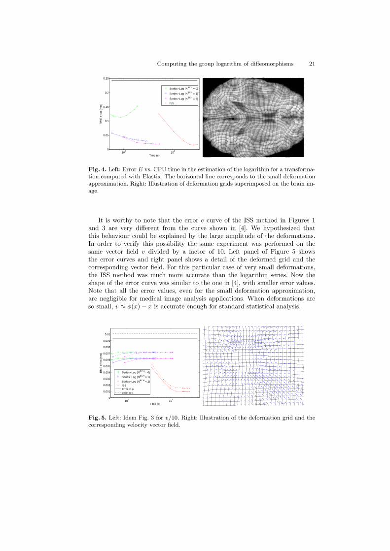
Fig. 4. Left: Error E vs. CPU time in the estimation of the logarithm for a transforma-tion computed with Elastix. The horizontal line corresponds to the small deformationapproximation. Right: Illustration of deformation grids superimposed on the brain im-age.
It is worthy to note that the error e curve of the ISS method in Figures 1and 3 are very different from the curve shown in [4]. We hypothesized thatthis behaviour could be explained by the large amplitude of the deformations.In order to verify this possibility the same experiment was performed on thesame vector field v divided by a factor of 10. Left panel of Figure 5 showsthe error curves and right panel shows a detail of the deformed grid and thecorresponding vector field. For this particular case of very small deformations,the ISS method was much more accurate than the logarithm series. Now theshape of the error curve was similar to the one in [4], with smaller error values.Note that all the error values, even for the small deformation approximation,are negligible for medical image analysis applications. When deformations areso small, v ≈ φ(x) − x is accurate enough for standard statistical analysis.
102
103
0
0.001
0.002
0.003
0.004
0.005
0.006
0.007
0.008
0.009
0.01
Time (s)
RM
S e
rror
(m
m)
Series−Log (NBCH = 0)
Series−Log (NBCH = 1)
Series−Log (NBCH = 2)ISSError in φerror in v
Fig. 5. Left: Idem Fig. 3 for v/10. Right: Illustration of the deformation grid and thecorresponding velocity vector field.

22 M. Bossa et al.
In our opinion, the accuracy of the ISS method for large diffeomorphismswas limited by the fact that the right way to interpolate diffeomorphisms isunknown. Interpolation of diffeomorphisms is performed in the squaring (self-composition) operation. The composition of diffeomorphisms using a kernel inter-polation scheme can provide non-diffeomorphic mappings. In contrast, velocityvector fields belong to a linear vector space, therefore they can be summed orinterpolated without leaving the space.
5 Conclusion
We presented a new algorithm for the estimation of the group logarithm ofarbitrary diffeomorphisms based on a series in terms of the Lie bracket and thegroup exponential. This method provided a much better accuracy-speed trade-off than the ISS method to estimate the vector field v defining a diffeomorphism.In particular, at least one term of the BCH formula was essential for the seriesto provide a significant improvement vs. the ISS method.
Once a fast algorithm to compute the logarithm is available, statistics of thespatial transformations mapping image instances to a given atlas can be easilycomputed by means of standard multivariate statistics on the tangent spaceassuming the Log-Euclidean framework. This will be the topic of future studies.
References
1. Grenander, U., Miller, M.I.: Computational anatomy: an emerging discipline. Q.Appl. Math. LVI(4) (1998) 617–694
2. Miller, M.I., Trouve, A., Younes, L.: On the metrics and Euler-Lagrange equationsof computational anatomy. Ann. Rev. Biomed. Eng 4 (2002) 375–405
3. Beg, M.F., Miller, M.I., Trouve, A., Younes, L.: Computing large deformationmetric mappings via geodesic flows of diffeomorphisms. IJCV 61 (2) (2005) 139–157
4. Arsigny, V., Commonwick, O., Pennec, X., Ayache, N.: Statistics on diffeomor-phisms in a Log-Euclidean framework. MICCAI 4190 (2006) 924 – 931
5. Winkel, R.: An Exponential Formula for Polynomial Vector Fields II. Lie Se-ries, Exponential Substituition, and Rooted Trees. Advances in Mathematics 147(1999) 260–303
6. Arsigny, V.: Processing Data in Lie Groups: An Algebraic Approach. Applica-tion to Non-Linear Registration and Diffusion Tensor MRI. PhD Thesis, Ecolepolytechnique (November 2006)
7. Bossa, M., Hernandez, M., Olmos, S.: Contributions to 3d diffeomorphic atlasestimation: Application to brain images. In: MICCAI. (2007) 667–674
8. Bossa, M., Zacur, E., Olmos, S.: Algorithms for computing the group exponentialof diffeomorphisms: performance evaluation. In: MMBIA Workshop at CVPR.(2008)
9. Glockner, H.: Fundamental problems in the theory of infinite-dimensional Liegroups. Journal of Geometry and Symmetry in Physics 5 (2006) 24–35

Computing the group logarithm of diffeomorphisms 23
10. Shattuck, D.W., Mirza, M., Adisetiyo, V., Hojatkashani, C., Salamon, G., Narr,K.L., Poldrack, R.A., Bilder, R.M., Toga, A.W.: Construction of a 3d probabilisticatlas of human cortical structures. NeuroImage 39(3) (2008) 1064–1080
11. Hernandez, M., Bossa, M.N., Olmos, S.: Registration of anatomical images usinggeodesic paths of diffeomorphisms parameterized with stationary vector fields. In:MMBIA Workshop at ICCV. (2007) 1–8
12. Staring, M., Klein, S., Pluim, J.P.: Nonrigid Registration with Tissue-DependentFiltering of the Deformation Field. Physics in Medicine and Biology 52(23) (De-cember 2007) 6879 – 6892
Comparing algorithms for diffeomorphic
registration: Stationary LDDMM and
Diffeomorphic Demons
Monica Hernandez1, Salvador Olmos1, and Xavier Pennec2
1 Communication Technologies Group (GTC)Aragon Institute of Engineering Research (I3A)
University of Zaragoza, Spain2 Asclepios, INRIA Sophia-Antipolis, France
Abstract. The stationary parameterization of diffeomorphisms is be-ing increasingly used in computational anatomy. In certain applicationsit provides similar results to the non-stationary parameterization alle-viating the computational charge. With this characterization for diffeo-morphisms, two different registration algorithms have been recently pro-posed: stationary LDDMM and diffeomorphic Demons. To our knowl-edge, their theoretical and practical differences have not been analyzedyet. In this article we provide a comparison between both algorithms ina common framework. To this end, we have studied the differences inthe elements of both registration scenarios. We have analyzed the sen-sitivity of the regularization parameters in the smoothness of the finaltransformations and compared the performance of the registration re-sults. Moreover, we have studied the potential of both algorithms for thecomputation of essential operations for further statistical analysis. Wehave found that both methods have comparable performance in terms ofimage matching although the transformations are qualitatively differentin some cases. Diffeomorphic Demons shows a slight advantage in termsof computational time. However, it does not provide as stationary LD-DMM the vector field in the tangent space needed to compute statisticsor exact inverse transformations.
Key words: Computational Anatomy, diffeomorphic registration, sta-tionary parameterization, LDDMM, diffeomorphic Demons
1 Introduction
Computational Anatomy aims at the study of the statistical variability of anatom-ical structures [1]. Anatomical information is encoded by the spatial transforma-tions existing between anatomical images and a template selected as reference [2].The analysis of these transformations allows modeling the anatomical variabil-ity of a population. In particular, statistical inference can be used in order toidentify anatomical differences between healthy and diseased groups or improvethe diagnosis of pathologies [3–5]. In the absence of a justified physical model
Comparing Stationary LDDMM and Diffeomorphic Demons 25
for inter-subject variability, diffeomorphisms (i.e. differentiable maps with differ-entiable inverse) provide a convenient mathematical framework to perform thisstatistical analysis [6, 7].
The Large Deformation Diffeomorphic Metric Mapping (LDDMM) has beenconsidered the reference paradigm for diffeomorphic registration in Computa-tional Anatomy [8, 9]. Diffeomorphisms are represented as end point of pathsparameterized by time-varying vector fields defined on the tangent space of a con-venient Riemannian manifold. Despite the solid foundations of the mathematicalframework, the high computational requirements have made this methodologynot much attractive for clinical applications where more efficient registrationalgorithms are usually preferred.
Recently, an alternative parameterization using stationary vector fields wasproposed [7]. This parameterization has been applied for diffeomorphic registra-tion in the variational problem studied in the LDDMM framework [10, 11] anddiffeomorphic Demons algorithm [12]. Stationary LDDMM is embedded into thetheoretical complexity of the LDDMM framework although it has resulted intoa much more efficient algorithm while providing similar registration results. Dif-feomorphic Demons is intended as an extension of original Demons algorithmsuitable for practical applications due to its efficiency and the quality of regis-tration results.
Although both methods have arisen from different backgrounds, they con-sider non-rigid registration as a diffusion process [13]. Moreover, they fit into thesame variational framework with the same image matching metric and similarcharacterizations for the diffeomorphic transformations. To our knowledge, thetheoretical and practical differences between both methods have not been ana-lyzed yet. In this article, we provide a comparison between both algorithms inthis common framework. The elements of the registration scenario (transforma-tion parameterization, image metric, regularization and optimization scheme)have been studied for both methods. In the experimental section we have an-alyzed the influence of the regularization parameters on the smoothness of thefinal transformations and compared the performance of the registration results.Moreover, we have studied the potential of both algorithms for the computa-tion of the inverse transformation and the logarithm which constitute essentialoperations for further statistical analysis.
The rest of the article is divided as follows. In Section 2 we study the ele-ments of stationary-LDDMM and diffeomorphic Demons. Results are presentedin Section 3. Finally, Section 4 presents the main concluding remarks.
2 Stationary LDDMM and Diffeomorphic Demons
In Computational Anatomy, diffeomorphic registration is defined as a variationalproblem involving the characterization of diffeomorphic transformations, an im-age metric to measure the similarity between the images after registration, aregularization constraint to favor stable numerical solutions, and an optimiza-tion technique to search for the optimal transformation in the space of valid

26 M. Hernandez et al.
diffeomorphisms. The transformation that deforms the source I0 into the targetI1 is computed from the minimization of the energy functional
E(ϕ) =1
σ2reg
· Ereg(ϕ) +1
σ2sim
· Esim(I0, I1, ϕ) (1)
where the weighting factors 1/σ2reg and 1/σ2
sim balance the energy contributionbetween regularization and matching. In this section we study the elementsof this registration scenario for stationary LDDMM [10, 11] and diffeomorphicDemons [12].
2.1 Characterization of diffeomorphic transformations
In the LDDMM framework [14, 8], transformations are assumed to belong to agroup of diffeomorphisms (i.e. differentiable maps ϕ : Ω → Ω with differentiableinverse) endowed with a Hilbert differentiable structure of Riemannian mani-fold, Diff(Ω). The tangent space V is a set of Sobolev class vector fields in Ω.The Riemannian metric is defined from the scalar product 〈v, w〉V = 〈Lv,Lw〉L2
where L is a linear invertible differentiable operator. Diffeomorphic transforma-tions are represented by the end point ϕ = φ(1) of paths of diffeomorphisms φ(t)parameterized by time-varying flows v(t) of vector fields in V from the solution ofthe transport equation φ(t) = v(t, φ(t)). The Sobolev structure in V guarantees
the existence of diffeomorphic solutions for these equations if∫ 1
0‖v(t)‖2
V dt <∞.
In stationary LDDMM [10, 11], paths of diffeomorphisms are parameterizedby constant-time flows of vector fields in V . This stationary parameterization isclosely related to the group structure defined in Diff(Ω) as the paths startingat the identity parameterized using stationary vector fields are exactly the one-parameter subgroups. Diffeomorphisms belonging to one-parameter subgroupscan be computed from the group exponential map Exp : V → Diff(Ω)
ϕ = Exp(w) (2)
where w constitutes the infinitesimal generator of the subgroup [7]. Thus, sta-tionary LDDMM restricts transformations to diffeomorphisms belonging to one-parameter subgroups. It has been shown that the set of diffeomorphisms obtainedwith the stationary parameterization do not comprise all diffeomorphisms inDiff(Ω) [15]. Nevertheless, the stationary parameterization has shown to pro-vide a performance similar to the more general non-stationary parameterizationon the registration of MRI brain anatomical images [11].
In diffeomorphic Demons [12], transformations are assumed to belong to agroup of diffeomorphisms Diff(Ω). In contrast to the LDDMM framework,no Riemannian structure is explicitly considered in Diff(Ω). Diffeomorphictransformations are represented as the composition of
ϕ = ψ Exp(u) (3)
Comparing Stationary LDDMM and Diffeomorphic Demons 27
where ψ is an element in Diff(Ω) and u is a vector field in Ω belonging toa convenient space of vector fields that guarantees the existence of the ex-ponential map and that the composition ψ Exp(u) remains in in Diff(Ω).This characterization restricts transformations to any element in Diff(Ω) thatcan be obtained by finite composition of exponentials of smooth vector fieldsϕ = Exp(u1) ... Exp(uN ).
2.2 Image metric
In stationary LDDMM the image matching energy is defined from
Esim(I0, I1, ϕ) = ‖I0 Exp(w)−1 − I1‖2L2 (4)
This term could be replaced by other energies proposed in non-stationary LD-DMM (as mutual information or cross correlation, among others [16, 17]). In gen-eral, the inverse of the minimizer of Esim(I0, I1, ·) is not minimizing the reciprocalenergy Esim(I1, I0, ·). Therefore, if the order of inputs is swapped the methoddoes not provide exact inverse transformations. Introducing inverse consistencyin the registration is important as the symmetry in the image matching shouldbe guaranteed by the diffeomorphic transformations used in most of Computa-tional Anatomy applications [17]. In stationary LDDMM, Exp(−w) and Exp(w)are exact inverse transformations. Therefore, the inverse consistent version ofthe image matching energy for stationary LDDMM simply corresponds to
Esim(I0, I1, ϕ) = ‖I0 Exp(w)−1 − I1‖2L2 + ‖I1 Exp(w) − I0‖
2L2 (5)
Diffeomorphic Demons is associated to the minimization of
Esim(I0, I1, ϕ) = ‖I0 ψ Exp(u) − I1‖2L2 (6)
The inverse consistent version of the image matching energy corresponds to 3
Esim(I0, I1, ϕ) = ‖I0 ψ Exp(u) − I1‖2L2 + ‖I1 ζ Exp(w) − I0‖
2L2 (7)
subject to (ψ Exp(u))−1 = ζ Exp(w). In this case, minimization involvesthe solution of a constrained optimization problem leading to a more complexalgorithm for general expressions of ψ and ζ.
2.3 Regularization energy
In stationary LDDMM the regularization term is defined as the norm in V ofthe infinitesimal generator w associated to the diffeomorphism ϕ, Ereg(ϕ) =‖w‖2
V = ‖Lw‖2L2 . The regularization term favors solutions to belong to one-
parameter subgroups with small energy preventing the transformations to be
3 The inverse (ψ Exp(u))−1 = Exp(−u) ψ−1 is written in the form given by Eq. 3
28 M. Hernandez et al.
non-diffeomorphic. The regularization term depends on the selection of the op-erator L that is usually related to the physical deformation model imposed onΩ. However, it remains an open question how to choose the best model in non-rigid registration algorithms [13, 10]. In this work we use the diffusive modelL = Id− α∇2. This selection restricts w to lie on a space of Sobolev class two.
In Demons framework regularization is externally imposed using Gaussiansmoothing on ϕ and u. This way, the physical deformation model assumed on Ωis roughly equivalent to the combination of a diffusive and a fluid model [18]. Itcan be shown that the effect of this Gaussian smoothing is equivalent to usingthe harmonic regularization Ereg(ϕ) = ‖Dϕ− I‖2
fro in Eq. 1 .
2.4 Optimization scheme
In stationary LDDMM, optimization is performed on the tangent space V (opti-mization on Hilbert spaces). Although classical gradient descent is usually usedfor numerical optimization [9, 11], more efficient and robust second-order tech-niques have been recently proposed [10, 19]. These methods are based on New-ton’s iterative scheme
wk+1 = wk − ǫ ·HwE(wk)−1 · ∇wE(wk) (8)
although they differ on the space where first and second order Gateaux (i.e.directional) derivatives are computed and the simplification of the Hessian termused to overcome the numerical problems posed by Newton’s method.
In [10], Gateaux derivatives are computed on the space of square integrablefunctions and Levenberg - Marquardt Newton’s simplification is used. Thus, theexpressions for the gradient and the Hessian are given by
(∇wE(w))L2 = 2 (L†L)w − (I0 Exp(w)−1 − I1) · ∇(I0 Exp(w)−1) (9)
(HwE(w))L2 = 2 (L†L) + ∇(I0 Exp(w)−1)T · ∇(I0 Exp(w)−1) (10)
With this approach, the action of the linear operator L†L has to be formulatedusing the matrix representation of the convolution. As a consequence, the algo-rithm results in a high dimensional matrix inversion problem with large compu-tational requirements. Although inversion is approached by solving a sparse sys-tem of linear equations combining Gauss-Seidel with multigrid techniques [20],the memory requirements for diffeomorphic registration hinder the execution instandard machines.
As an alternative, it was proposed in [19] to compute Gateaux derivatives inthe space V using a Gauss-Newton simplification, which leads to
(∇wE(w))V = 2 w − (L†L)−1((I0 Exp(w)−1 − I1) · ∇(I0 Exp(w)−1))(11)
(HwE(w))V = 2 IR3 + (L†L)−2(∇(I0 Exp(w)−1)T · ∇(I0 Exp(w)−1))(12)
With this approach, the action of the operators (L†L)−1 and (L†L)−2 can beformulated using convolution and the update of Eq. 8 can be computed usingpointwise operations with smaller memory requirements.
Comparing Stationary LDDMM and Diffeomorphic Demons 29
Apart from the computational requirements, Beg et al. provided an additionalargument supporting optimization on space V rather than on L2 [9]. The linearoperator K = (L†L)−1 is a compact operator in V . Using results from F. Riesz’sspectral theory of compact operators, there exists an orthonormal basis (n)n∈N
in L2 with corresponding singular values (λn)n∈N such that
K =∑
n∈N
(λn〈·,n〉L2) ·n (13)
and λn → 0 as n → ∞ due to operator compactness. The expansion of thegradient expressions in this basis yields 4
(∇wE(w))L2 =∑
n∈N
(
1
λn
〈2w,n〉L2 + 〈−b,n〉L2
)
·n (14)
(∇wE(w))V =∑
n∈N
(〈2w,n〉L2 + λn〈−b,n〉L2) ·n (15)
where b = (I0 Exp(w)−1 − I1) · ∇(I0 Exp(w)−1). Therefore, whereas theaction of the linear operator (L†L)−1 in Eq. 11 remains bounded, the action of(L†L) Eq. 9 results into a high frequency components amplification leading tonumerical instabilities in the computations.
In diffeomorphic Demons optimization is performed on the group of diffeo-morphisms Diff(Ω) (optimization on Lie groups) using the iterative scheme
uk+1 =I0 ϕ
k − I1‖∇(I0 ϕk) ·Dϕk‖2
L2 + (I0 ϕk − I1)2/τ2· (∇(I0 ϕ
k) · (Dϕk))(16)
ϕk+1 = ϕk Exp(ǫ · uk+1) (17)
where second order techniques are used for the computation of uk [12].Regularization is performed at the end of each iteration by smoothing the up-dated uk and ϕk using Gaussian filters of standard deviation σu and σϕ, re-spectively. Moreover, the term (I0 ϕ
k − I1)2/τ2 also contributes to the regu-
larization by enforcing the numerical stability of the optimization scheme andcontrolling the maximum update step length. This term can be seen as a Leven-berg - Maquardt approximation of Gauss-Newton’s method. Leaving aside thecommon variational formulation provided in this work, an identical optimizationscheme can be obtained from a variational formulation resulting from the intro-duction of a hidden variable that controls the correspondences between ϕ andthe true transformation [21].
Alternative to this usual Gauss-Newton optimization, the efficient secondorder scheme introduced in [22] was used in [12]. This led to replacing the term∇(I0 ϕ) in Eq. 16 by its symmetric version ∇(I0 ϕ) + ∇I1. This was shownto improve the rate of convergence with respect to the original Gauss-Newton
4 Analogous conclusions can be inferred from expanding the bilinear form associatedto Hessian expressions in this basis.

30 M. Hernandez et al.
Table 1. Stationary LDDMM registration. Average and standard deviation of theRSSD (%) (upper row) and Jmin (lower row) for different values of the regularizationparameters α and 1/σ2
sim. The optimal result for each algorithm is outlined in bold-face. Non-diffeomorphic results are outlined in italics. Note that the algorithms do notconverge for values α of order 0.0001.
Inverse consistent LDDMM. RSSD = 1
2
‖I0ϕ−I1‖
2
2+‖I1ϕ−1
−I0‖
2
2
‖I0−I1‖2
2
.P
PP
PPP
1/σ2
sim
α1.0 0.01 0.0050 0.0025 0.0010 0.0001
1.0e391.56 ± 3.04 30.53 ± 3.76 21.51 ± 2.37 17.42 ± 4.16 12.18 ± 3.17 100.00 ± 0.00
0.60 ± 0.24 0.44 ± 0.11 0.27 ± 0.07 0.17 ± 0.06 -0.17 ± 0.64 1.00 ± 0.00
1.0e490.97 ± 3.11 24.70 ± 3.10 17.55 ± 2.10 13.88 ± 4.13 9.72 ± 3.72 100.00 ± 0.00
0.59 ± 0.24 0.31 ± 0.15 0.19 ± 0.08 0.10 ± 0.05 -3.97 ± 12.28 1.00 ± 0.00
1.0e590.97 ± 3.11 24.70 ± 3.10 17.55 ± 2.10 13.82 ± 4.00 9.61 ± 3.57 100.00 ± 0.00
0.59 ± 0.24 0.31 ± 0.15 0.19 ± 0.08 0.10 ± 0.05 -3.99 ± 12.28 1.00 ± 0.00
Symmetric gradient LDDMM. RSSD =‖I0ϕ−I1‖
2
2
‖I0−I1‖2
2
.
PP
PP
PP1/σ2
sim
α1.0 0.01 0.0050 0.0025 0.0010 0.0001
1.0e391.66 ± 2.88 30.44 ± 3.44 22.02 ± 2.33 15.79 ± 1.68 10.88 ± 1.21 100.00 ± 0.00
0.65 ± 0.22 0.44 ± 0.09 0.26 ± 0.08 0.11 ± 0.07 0.02 ± 0.02 1.00 ± 0.00
1.0e491.11 ± 2.73 28.61 ± 3.44 20.99 ± 2.38 14.81 ± 1.59 10.09 ± 1.35 100.00 ± 0.00
0.63 ± 0.23 0.39 ± 0.12 0.23 ± 0.10 0.10 ± 0.07 0.01 ± 0.01 1.00 ± 0.00
1.0e591.11 ± 2.73 28.83 ± 3.62 21.49 ± 2.46 15.38 ± 2.74 10.09 ± 1.34 100.00 ± 0.00
0.63 ± 0.23 0.39 ± 0.12 0.25 ± 0.10 0.11 ± 0.07 0.01 ± 0.01 1.00 ± 0.00
scheme. It should be noted that the efficient second order scheme can be alsointroduced in Gauss-Newton LDDMM optimization by modifying Eqs. 9 to 12.In the experimental section, we will explore its influence in registration results.
3 Results
3.1 Datasets and experimental setting
A set of 18 T1-MRI images from the Internet Brain Segmentation Repository(IBSR) were used for comparing the performance of the registration algorithms.The images size was 256 × 256 × 128 with a voxel size of 0.94 × 0.94 × 1.5.The images were acquired at the Massachusetts General Hospital and are freelyavailable at http://www.cma.mgh.harvard.edu/ibsr/data.html.
In our experiments, one of the images was randomly selected as a templateand the remaining of the datasets were registered to this template using sta-tionary LDDMM and diffeomorphic Demons algorithms. Both algorithms werestopped when the magnitude of the update was negligible or after a maximumof 100 iterations. The selection of the optimal regularization parameters is pre-sented below. Other parameters were fixed to typical values used in previousworks [10–12]. The parameter ǫ controls the step size made along the searchdirection in both methods. It was estimated using a backtracking inexact line-search strategy starting from ǫ = 1 for each iteration (see [19] for more details).
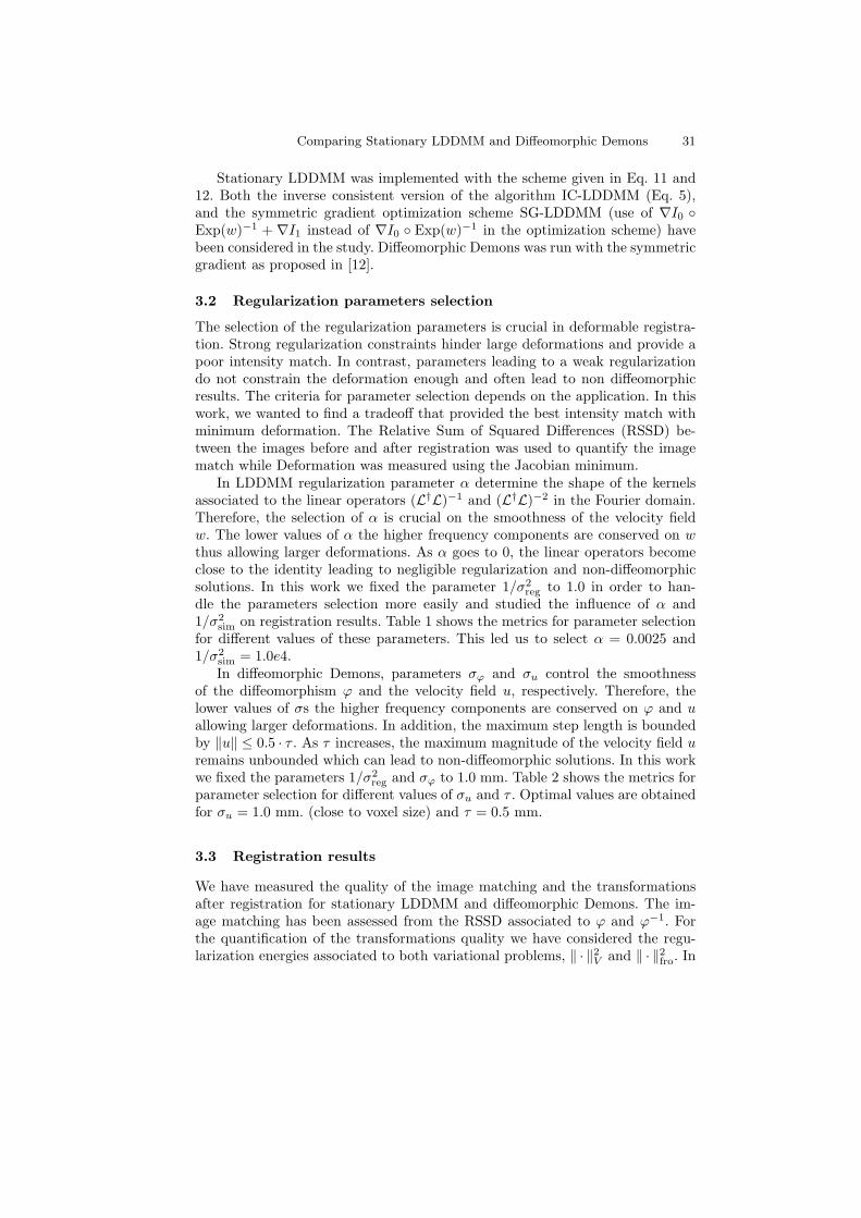
Comparing Stationary LDDMM and Diffeomorphic Demons 31
Stationary LDDMM was implemented with the scheme given in Eq. 11 and12. Both the inverse consistent version of the algorithm IC-LDDMM (Eq. 5),and the symmetric gradient optimization scheme SG-LDDMM (use of ∇I0 Exp(w)−1 + ∇I1 instead of ∇I0 Exp(w)−1 in the optimization scheme) havebeen considered in the study. Diffeomorphic Demons was run with the symmetricgradient as proposed in [12].
3.2 Regularization parameters selection
The selection of the regularization parameters is crucial in deformable registra-tion. Strong regularization constraints hinder large deformations and provide apoor intensity match. In contrast, parameters leading to a weak regularizationdo not constrain the deformation enough and often lead to non diffeomorphicresults. The criteria for parameter selection depends on the application. In thiswork, we wanted to find a tradeoff that provided the best intensity match withminimum deformation. The Relative Sum of Squared Differences (RSSD) be-tween the images before and after registration was used to quantify the imagematch while Deformation was measured using the Jacobian minimum.
In LDDMM regularization parameter α determine the shape of the kernelsassociated to the linear operators (L†L)−1 and (L†L)−2 in the Fourier domain.Therefore, the selection of α is crucial on the smoothness of the velocity fieldw. The lower values of α the higher frequency components are conserved on wthus allowing larger deformations. As α goes to 0, the linear operators becomeclose to the identity leading to negligible regularization and non-diffeomorphicsolutions. In this work we fixed the parameter 1/σ2
reg to 1.0 in order to han-dle the parameters selection more easily and studied the influence of α and1/σ2
sim on registration results. Table 1 shows the metrics for parameter selectionfor different values of these parameters. This led us to select α = 0.0025 and1/σ2
sim = 1.0e4.In diffeomorphic Demons, parameters σϕ and σu control the smoothness
of the diffeomorphism ϕ and the velocity field u, respectively. Therefore, thelower values of σs the higher frequency components are conserved on ϕ and uallowing larger deformations. In addition, the maximum step length is boundedby ‖u‖ ≤ 0.5 · τ . As τ increases, the maximum magnitude of the velocity field uremains unbounded which can lead to non-diffeomorphic solutions. In this workwe fixed the parameters 1/σ2
reg and σϕ to 1.0 mm. Table 2 shows the metrics forparameter selection for different values of σu and τ . Optimal values are obtainedfor σu = 1.0 mm. (close to voxel size) and τ = 0.5 mm.
3.3 Registration results
We have measured the quality of the image matching and the transformationsafter registration for stationary LDDMM and diffeomorphic Demons. The im-age matching has been assessed from the RSSD associated to ϕ and ϕ−1. Forthe quantification of the transformations quality we have considered the regu-larization energies associated to both variational problems, ‖ · ‖2
V and ‖ · ‖2fro. In

32 M. Hernandez et al.
Table 2. Diffeomorphic Demons registration. Average and standard deviation of theRSSD (%) (upper row) and Jmin (lower row) for different values of the regularizationparameters σsim and τ . The optimal result is outlined in boldface. Non-diffeomorphicresults are outlined in italics.
Diffeomorphic Demons. RSSD =‖I0ϕ−I1‖
2
2
‖I0−I1‖2
2
.
HH
HHτσu 1.0 1.5 2.0 2.5 3.0
0.514.88 ± 1.74 20.91 ± 2.50 31.58 ± 3.67 40.71 ± 4.34 48.15 ± 4.61
0.07 ± 0.03 0.15 ± 0.04 0.31 ± 0.05 0.47 ± 0.06 0.59 ± 0.06
1.09.95 ± 1.18 13.99 ± 1.69 21.73 ± 2.73 29.37 ± 3.72 36.19 ± 4.47
0.00 ± 0.00 0.02 ± 0.02 0.11 ± 0.05 0.23 ± 0.07 0.35 ± 0.09
2.010.91 ± 1.79 12.60 ± 1.26 18.06 ± 2.15 24.51 ± 3.01 30.59 ± 3.75
-0.01 ± 0.02 -0.00 ± 0.01 0.02 ± 0.02 0.10 ± 0.04 0.19 ± 0.07
stationary LDDMM ϕ and ϕ−1 have been computed from the exponential mapof w [7]. In diffeomorphic Demons the inverse diffeomorphism and the vectorsin the tangent space have been computed as proposed in [7]. Table 3 presentsthe results of these metrics. In addition, Figure 1 shows the registration resultsfor the experiment with the largest ventricle deformation. Figure 2 shows somerepresentative examples of the image-based energy curves during optimization.
3.4 Efficiency
Our experiments were performed on a 2.33 GHZ machine with a C++ imple-mentation based on the ITK library. We found that the computation time periteration was approximately 41.54 seconds for diffeomorphic Demons, 53.23 sec-onds for SG-LDDMM and 90.64 seconds for IC-LDDMM. However, it should benoted that if we were also interested in computing the inverse diffeomorphism orthe logarithm from the output of diffeomorphic Demons, the computation timeof the inverse diffeomorphism would take in average 5 706± 34 seconds whereasthe computation time for the logarithm would take 17 463 ± 10 681 seconds.
Table 3. Average and standard deviation of the metrics associated to the registrationresults. With IC-LDDMM and SG-LDDMM we indicate the inverse consistent and thesymmetric gradient version of LDDMM, respectively.
RSSD(I0ϕ,I1) (%) RSSD(I1ϕ−1,I0)
(%) ‖ · ‖2
V ‖ · ‖2
fro
IC-LDDMM 13.42 ± 4.23 14.43 ± 4.24 140.52 ± 28.84 0.17 ± 0.05
SG-LDDMM 14.81 ± 1.59 15.47 ± 2.50 166.62 ± 12.05 0.20 ± 0.03
Demons 14.88 ± 1.74 19.00 ± 4.72 2626.70 ± 6069.90 0.13 ± 0.01
4 Discussion and conclusions
In this article we presented a theoretical and experimental comparison of twodiffeomorphic registration techniques that use stationary vector fields to com-pute diffeomorphisms. We analyzed the differences in the elements of both reg-istration scenarios, studied the influence of the regularization parameters on thequality of the final transformations and compared the performance of the regis-tration results. For stationary LDDMM, we considered both the inverse consis-tent version of the algorithm and the symmetric gradient optimization scheme.

Comparing Stationary LDDMM and Diffeomorphic Demons 33
Fig. 1. Visual assessment of diffeomorphic registration algorithms. First row shows axial slices of thereference (left) and the deforming image (middle) together with the differences before registration(right). Second row shows the differences after registration with IC-LDDMM (left), SG-LDDMM(middle) and Demons (right). Third row shows the corresponding diffeomorphisms.
For diffeomorphic Demons we just considered the symmetric gradient optimiza-tion scheme. We found that parameters α in LDDMM and τ in diffeomorphicDemons were strongly influencing the smoothness of the final transformation.There even exist combinations of such parameters that provide non diffeomor-phic transformations. It seems that non diffeomorphic transformations at RSSDapproximately below 13% can be achieved in our datasets. This should be takeninto account in parameter selection for specific applications.
We found that both algorithms provided a similar intensity matching (aver-age RSSD ranging from 13.42 to 14.88 %). However, in some cases, both algo-rithms locally showed different performance. As can be appreciated in Figure 1,larger deformations in stationary LDDMM yielded a higher image matching inlocations such as, for example, ventricles tails. SG-LDDMM provided a slightlybetter consistent inverse image matching than diffeomorphic Demons (averageRSSD of 15.5 for stationary LDDMM vs RSSD of 19.0 for Demons). In this case,average RSSD differences between methods were statistically different for diffeo-morphic Demons. The regularization energy in V showed to be much higher inthe case of diffeomorphic Demons. This may be due to the bad numerical con-
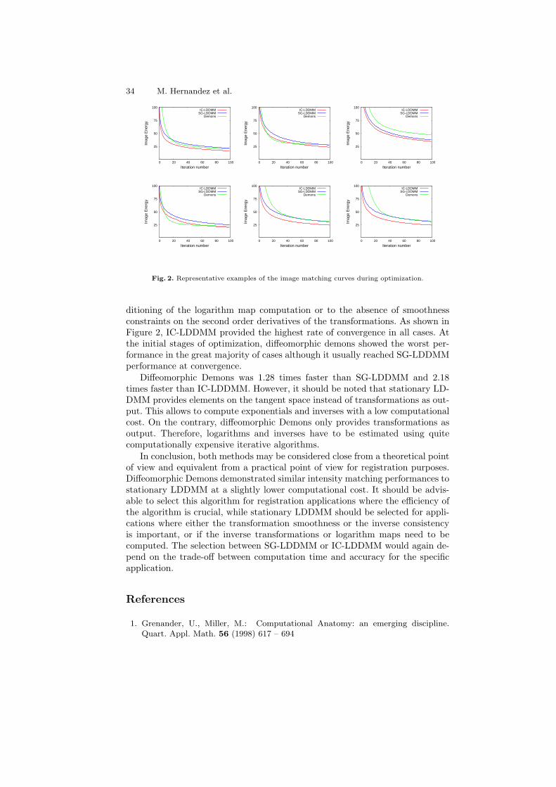
34 M. Hernandez et al.
25
50
75
100
0 20 40 60 80 100
Imag
e E
nerg
y
Iteration number
IC-LDDMMSG-LDDMM
Demons
25
50
75
100
0 20 40 60 80 100
Imag
e E
nerg
y
Iteration number
IC-LDDMMSG-LDDMM
Demons
25
50
75
100
0 20 40 60 80 100
Imag
e E
nerg
y
Iteration number
IC-LDDMMSG-LDDMM
Demons
25
50
75
100
0 20 40 60 80 100
Imag
e E
nerg
y
Iteration number
IC-LDDMMSG-LDDMM
Demons
25
50
75
100
0 20 40 60 80 100Im
age
Ene
rgy
Iteration number
IC-LDDMMSG-LDDMM
Demons
25
50
75
100
0 20 40 60 80 100
Imag
e E
nerg
y
Iteration number
IC-LDDMMSG-LDDMM
Demons
Fig. 2. Representative examples of the image matching curves during optimization.
ditioning of the logarithm map computation or to the absence of smoothnessconstraints on the second order derivatives of the transformations. As shown inFigure 2, IC-LDDMM provided the highest rate of convergence in all cases. Atthe initial stages of optimization, diffeomorphic demons showed the worst per-formance in the great majority of cases although it usually reached SG-LDDMMperformance at convergence.
Diffeomorphic Demons was 1.28 times faster than SG-LDDMM and 2.18times faster than IC-LDDMM. However, it should be noted that stationary LD-DMM provides elements on the tangent space instead of transformations as out-put. This allows to compute exponentials and inverses with a low computationalcost. On the contrary, diffeomorphic Demons only provides transformations asoutput. Therefore, logarithms and inverses have to be estimated using quitecomputationally expensive iterative algorithms.
In conclusion, both methods may be considered close from a theoretical pointof view and equivalent from a practical point of view for registration purposes.Diffeomorphic Demons demonstrated similar intensity matching performances tostationary LDDMM at a slightly lower computational cost. It should be advis-able to select this algorithm for registration applications where the efficiency ofthe algorithm is crucial, while stationary LDDMM should be selected for appli-cations where either the transformation smoothness or the inverse consistencyis important, or if the inverse transformations or logarithm maps need to becomputed. The selection between SG-LDDMM or IC-LDDMM would again de-pend on the trade-off between computation time and accuracy for the specificapplication.
References
1. Grenander, U., Miller, M.: Computational Anatomy: an emerging discipline.Quart. Appl. Math. 56 (1998) 617 – 694

Comparing Stationary LDDMM and Diffeomorphic Demons 35
2. Grenander, U.: General pattern theory. Oxford University Press (1994)3. Thompson, P.M., et al.: Detection and mapping of abnormal brain structure with
a probabilistic atlas of cortical surfaces. J. Comp. Ass. Tomography 21(4) (1997)567 – 581
4. Thompson, P.M., et al.: Cortical change in Alzheimer’s disease detected with adisease-specific population-based brain atlas. Cerebral Cortex 11(1) (2001) 1 – 16
5. Miller, M.I.: Computational anatomy: shape, growth, and atrophy comparison viadiffeomorphisms. Neuroimage 23 (2004) 19–33
6. Miller, M.I., Trouve, A., Younes, L.: Geodesic shooting for computational anatomy.J. Math. Imaging Vis. 24 (2006) 209–228
7. Arsigny, V., Commonwick, O., Pennec, X., Ayache, N.: Statistics on diffeomor-phisms in a Log-Euclidean framework. MICCAI’06, LNCS 4190 (2006) 924 –931
8. Dupuis, P., Grenander, U., Miller, M.: Variational problems on flows of diffeomor-phisms for image matching. Quart. Appl. Math. (1998) 587 – 600
9. Beg, M., Miller, M., Trouve, A., Younes, L.: Computing large deformation metricmappings via geodesic flows of diffeomorphisms. Int. J. Comput. Vis. 61 (2) (2005)139–157
10. Ashburner, J.: A fast diffeomorphic image registration algorithm. Neuroimage38(1) (2007) 95 – 113
11. Hernandez, M., Bossa, M.N., Olmos, S.: Registration of anatomical images us-ing geodesic paths of diffeomorphisms parameterized with stationary vector fields.MMBIA’07 (2007)
12. Vercauteren, T., Pennec, X., Perchant, A., Ayache, N.: Diffeomorphic image reg-istration with the demons algorithm. MICCAI’07, LNCS 4792 (2007) 319 – 326
13. Modersitzki, J.: Numerical methods for image registration. Oxford UniversityPress (2004)
14. Trouve, A.: Diffeomorphism groups and pattern matching in image analysis. Int.J. Comput. Vis. 28 (1998) 213 – 221
15. Grabowski, J.: Free subgroups of diffeomorphism groups. Fundam. Math. 131(1988) 103 – 121
16. Lorenzen, P., Prastawa, M., Davis, B., Gerig, G., Bullitt, E., Joshi, S.: Multi-modalimage set registration and atlas formation. Med. Image. Anal. 10 (2006) 440 – 451
17. Avants, B.B., Epstein, C.L., Grossman, M., Gee, J.C.: Symmetric dieomorphicimage registration with cross-correlation: Evaluating automated labeling of elderlyand neurodegenerative brain. Med. Image. Anal. 12 (1998) 26 – 41
18. Pennec, X., Cachier, P., Ayache, N.: Understanding the Demons algorithm: non-rigid registration by gradient descent. MICCAI’99, LNCS 1679 (1999) 597 – 605
19. Hernandez, M., Olmos, S.: Gauss-Newton optimization in diffeomorphic registra-tion. ISBI’08 (2008)
20. Press, W.H., Teukolsky, S.A., Vetterling, W.T., Flannery, B.P.: Numerical recipesin C: the art of scientific computing. Cambridge University Press, Cambridge(1992)
21. Cachier, P., Bardinet, E., Dormont, D., Pennec, X., Ayache, N.: Iconic featurebased nonrigid registration: the PASHA algorithm. Comput. Vis. Image Underst.89 (2003) 272 – 298
22. Malis, E.: Improving vision-based control using efficient second-order minimizationtechniques. IEEE Int. Conf. Robot. Aut. 2 (2004) 1843 – 1848
Brain Mapping with the Ricci Flow Conformal
Parameterization and Multivariate Statistics on
Deformation Tensors
Yalin Wang1,2, Xiaotian Yin3, Jie Zhang4, Xianfeng Gu3, Tony F. Chan2, PaulM. Thompson1, and Shing-Tung Yau5
1 Lab. of Neuro Imaging, UCLA School of Medicine, Los Angeles, CA 90095, USA,2 Mathematics Department, UCLA, Los Angeles, CA 90095, USA,
3 Computer Science Dept., SUNY at Stony Brook, Stony Brook, NY 11794, USA,4 Mathematics Department, Zhejiang University, Hangzhou, China
5 Department of Mathematics, Harvard University, Cambridge, MA 02138, USA,[email protected]
Abstract. By solving the Yamabe equation with the discrete surfaceRicci flow method, we can conformally parameterize a multiple bound-ary surface by a multi-hole disk. The resulting parameterizations do nothave any singularities and they are intrinsic and stable. For applicationsin brain mapping research, first, we convert a cortical surface modelinto a multiple boundary surface by cutting along selected anatomicallandmark curves. Secondly, we conformally parameterize each corticalsurface using a multi-hole disk. Inter-subject cortical surface matchingis performed by solving a constrained harmonic map in the canonicalparameter domain. To map group differences in cortical morphometry,we then compute a manifold version of Hotelling’s T 2 test on the Ja-cobian matrices. Permutation testing was used to estimate statisticalsignificance. We studied brain morphology in 21 patients with WilliamsSyndrome (WE) and 21 matched healthy control subjects with the pro-posed method. The results demonstrate our algorithm’s potential powerto effectively detect group differences on cortical surfaces.
1 Introduction
Surface-based modeling is valuable in brain imaging to help analyze anatomicalshape, to detect abnormalities of cortical surface folding, and to statistically com-bine or compare 3D anatomical models across subjects. Even so, a direct mappingbetween two 3D surfaces from different subjects is challenging to compute. Of-ten, higher order correspondences must be enforced between specific anatomicalpoints, curved landmarks, or subregions lying within the two surfaces. This isoften achieved by first mapping each of the 3D surfaces to canonical parameterspaces such as a sphere [1, 2] or a planar domain [3]. A flow, computed in theparameter space of the two surfaces [4, 5], then induces a correspondence fieldin 3D. This flow can be constrained using anatomic landmark points or curves,by constraining the mapping of surface regions represented implicitly using level
Brain Mapping with the Ricci Flow 37
sets [3], or by using currents to represent anatomical variation [6] Feature cor-respondence between two surfaces can be optimized by using the L2-norm tomeasure differences in curvature profiles or convexity [1] or by using mutualinformation to align scalar fields of various differential geometric parameters de-fined on the surface [7]. Artificial neural networks may also be used to rule out orfavor certain types of feature matches [8]. Finally, correspondences may be de-termined by using a minimum description length (MDL) principle, based on thecompactness of the covariance of the resulting shape model [9]. Anatomicallyhomologous points can then be forced to match across a dataset. Thodberg [10]identified problems with early MDL approaches and extended them to an MDLappearance model, when performing unsupervised image segmentation.
All oriented surfaces have conformal structures. The conformal structure is, insome respects, more flexible than the Riemannian metric but places more restric-tions on the the surface morphology than the topological structure. The Ricciflow method can conformally map an open boundary surface to a multi-holedisk [11]. Compared with other conformal parameterization methods [12–15],the Ricci flow method can handle cortical surfaces with complicated topologieswithout singularities. The continuous Ricci flow conformally deforms a Rieman-nian metric on a smooth surface such that the Gaussian curvature evolves likea heat diffusion process. In the discrete case, with the circle packing metric, theRicci flow can be formulated in a variational setting and solved by the Newtonmethod [11].
Tensor-based morphometry is widely used in computational anatomy as ameans to understand shape variation between structural brain images. Tech-niques based on Riemannian manifolds to compare deformation tensors or strainmatrices were introduced in [16–18]. In [19], the full deformation tensors wereused in the context of tensor-based morphometry. In a conformal parameteri-zation, the original metric tensor is preserved up to a constant. The conformalparametrization provides an ideal framework to apply tensor based morphom-etry on surfaces, to help understand shape variation between structural brainimages.
In this paper, we use the Ricci flow method to compute a conformal mappingbetween cortical surfaces and a multi-hole surface. Then we compute a directcortical surface correspondence by computing a constrained harmonic map onthe parameter domain. We apply multivariate statistics to the Jacobian matricesto study cortical surface variation between a group of patients with Williamssyndrome (WS) and a group of healthy control subjects. WS is a genetic disorderin which the cortex develops abnormally, but the scope and type of systematicdifferences is unknown [20]. In our experimental results, we identified severalsignificantly different areas on the left and right cortical surfaces between WSpatients and control subjects.

38 Y. Wang et al.
2 Ricci Flow Conformal Parameterization
In this section, we introduce the theory of Ricci flow in the continuous setting,and then generalize it to the discrete setting.
2.1 Ricci Flow on Continuous Surfaces
Riemannian Metric and Gaussian Curvature All the concepts used heremay be found, with detailed explanations, in [21]. Suppose S is a C2 smoothsurface embedded in R
3 with local parameters (u1, u2). Let r(u1, u2) be a pointon S and dr = r1du1 + r2du2 be the tangent vector defined at that point, wherer1, r2 are the partial derivatives of r with respect to u1 and u2, respectively. TheRiemannian metric or the first fundamental form is:
< dr, dr >=∑
< ri, rj > duiduj , i, j = 1, 2. (1)
The Gauss map G : S → S2 from the surface S to the unit sphere S
2 mapseach point p on the surface to its normal n(p). The Gaussian curvature K(p) is
defined as the Jacobian of the Gauss map. Intuitively, it is the ratio between theinfinitesimal area of the image of the Gauss map and the infinitesimal area onthe original surface.
The total curvature of a compact surface is determined by the topology ofthe surface:
∫
SKdA +
∫
∂Skgds = 2πχ(S), where ∂S is the boundary of the
surface S, kg is the geodesic curvature, and χ(S) is the Euler characteristic ofthe surface (an integer).
Fig. 1. Properties of Conformal Mapping: Conformal mappings transform in-finitesimal circles to infinitesimal circles and preserve the intersection angles amongthe circles. Here, infinitesimal circles are approximated by finite ones.
Conformal deformation Let S be a surface embedded in R3. S has a
Riemannian metric induced from the Euclidean metric of R3, denoted by g.
Suppose u : S → R is a scalar function defined on S. It can be verified thatg = e2ug is also a Riemannian metric on S, and angles measured by g are equalto those measured by g. We say g is a conformal deformation from g. Figure

Brain Mapping with the Ricci Flow 39
1 shows that a conformal deformation maps infinitesimal circles to infinitesimalcircles and preserves their intersection angles.
When the Riemannian metric is conformally deformed, curvatures will also bechanged accordingly. Suppose g is changed to g = e2ug, the Gaussian curvaturewill become K = e−2u(−∆gu+K), where ∆g is the Laplacian-Beltrami operatorunder the original metric g. The geodesic curvature will become k = e−u(∂ru +k), where r is the tangent vector orthogonal to the boundary.
Smooth Surface Ricci Flow Suppose S is a smooth surface with a Rieman-nian metric g. The Ricci flow deforms the metric g(t) according to the Gaussiancurvature K(t) (induced by g(t) itself), where t is the time parameter
dgij(t)
dt= −2K(t)gij(t). (2)
If we replace the metric in Eq. 2 with g(t) = e2u(t)g(0), then the Ricci flow canbe simplified as du(t)/dt = −2K(t), which states that the metric should changeaccording to the curvature.
The Ricci flow can be easily modified to compute a metric with a user-defined
curvature K : du(t)/dt = 2(K − K). The resulting metric g(∞) will induce theuser-defined curvature K.
The Ricci flow has been proven to converge. For surfaces with non-positiveand positive Euler numbers, the proofs were given by Hamilton [22] and Chow[23] respectively. For a closed surface, if the total area is preserved during theflow, the Ricci flow will converge to a metric such that the Gaussian curvatureis constant everywhere.
2.2 Ricci Flow on Discrete Surfaces
In engineering fields, smooth surfaces are often approximated by simplicial com-plexes (triangle meshes). Key concepts, such as the metric, curvature, and con-formal deformation in the continuous setting can be generalized to the discretesetting. We denote a triangle mesh as Σ, the mesh boundary as ∂Σ, a vertex setas V , an edge set as E, and a face set as F . eij represents the edge connectingvertices vi and vj , and fijk denotes the face formed by vi, vj , and vk.
Discrete Riemannian Metric and Gaussian Curvature A Riemannianmetric on a mesh Σ is a piecewise constant metric with cone singularities atvertices.
The edge lengths of a mesh Σ are sufficient to define the Riemannian metric,l : E → R
+, as long as for each face fijk, the edge lengths satisfy the triangleinequality: lij + ljk > lki.
The discrete Gaussian curvature Ki on a vertex vi ∈ Σ can be computedfrom the angle deficit,
Ki =
2π −∑
fijk∈F θjki , vi 6∈ ∂Σ
π −∑
fijk∈F θjki , vi ∈ ∂Σ
(3)
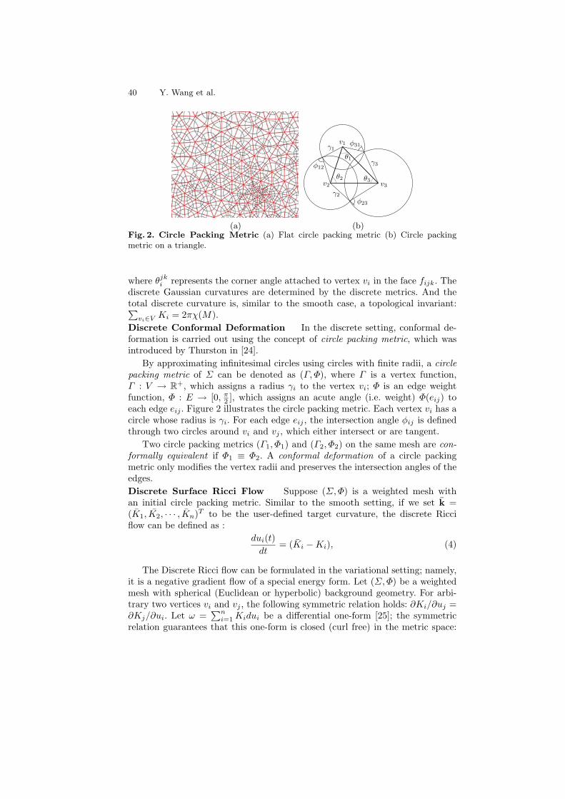
40 Y. Wang et al.
v1
v2 v3
φ12
φ23
φ31γ1
γ2
γ3
θ1
θ2 θ3
(a) (b)Fig. 2. Circle Packing Metric (a) Flat circle packing metric (b) Circle packingmetric on a triangle.
where θjki represents the corner angle attached to vertex vi in the face fijk. The
discrete Gaussian curvatures are determined by the discrete metrics. And thetotal discrete curvature is, similar to the smooth case, a topological invariant:∑
vi∈V Ki = 2πχ(M).
Discrete Conformal Deformation In the discrete setting, conformal de-formation is carried out using the concept of circle packing metric, which wasintroduced by Thurston in [24].
By approximating infinitesimal circles using circles with finite radii, a circle
packing metric of Σ can be denoted as (Γ,Φ), where Γ is a vertex function,Γ : V → R
+, which assigns a radius γi to the vertex vi; Φ is an edge weightfunction, Φ : E → [0, π
2 ], which assigns an acute angle (i.e. weight) Φ(eij) toeach edge eij . Figure 2 illustrates the circle packing metric. Each vertex vi has acircle whose radius is γi. For each edge eij , the intersection angle φij is definedthrough two circles around vi and vj , which either intersect or are tangent.
Two circle packing metrics (Γ1, Φ1) and (Γ2, Φ2) on the same mesh are con-
formally equivalent if Φ1 ≡ Φ2. A conformal deformation of a circle packingmetric only modifies the vertex radii and preserves the intersection angles of theedges.
Discrete Surface Ricci Flow Suppose (Σ,Φ) is a weighted mesh withan initial circle packing metric. Similar to the smooth setting, if we set k =(K1, K2, · · · , Kn)T to be the user-defined target curvature, the discrete Ricciflow can be defined as :
dui(t)
dt= (Ki − Ki), (4)
The Discrete Ricci flow can be formulated in the variational setting; namely,it is a negative gradient flow of a special energy form. Let (Σ,Φ) be a weightedmesh with spherical (Euclidean or hyperbolic) background geometry. For arbi-trary two vertices vi and vj , the following symmetric relation holds: ∂Ki/∂uj =∂Kj/∂ui. Let ω =
∑ni=1 Kidui be a differential one-form [25]; the symmetric
relation guarantees that this one-form is closed (curl free) in the metric space:
Brain Mapping with the Ricci Flow 41
dω = 0. Then by Stokes theorem, the following integration is path independent:
f(u) =
∫ u
u0
n∑
i=1
(Ki − Ki)dui, (5)
where n is the number of vertices, ui = log(γi), γi is the radius associated withedge i, and u0 is an arbitrary initial metric.
The above integration (Eq. 5) is called the discrete Ricci energy, which is well-defined. The discrete Ricci energy has been proved to be strictly convex (i.e., itsHessian is positive definite) in [26]. The global minimum uniquely exists, whichgives the desired discrete metric that induces k. The discrete Ricci flow is thenegative gradient flow of this energy, and it converges to the global minimum.
As in [11], the discrete surface Ricci flow method was used to solve theYamabe equation [11] and conformally map an open boundary cortical surfaceto a multi-hole disk.
3 Multivariate Statistics on Deformation Tensors
3.1 Derivative Map
Suppose φ : S1 → S2 is a map from the surface S1 to the surface S2. In orderto simplify the formulation, we use the isothermal coordinates of both surfacesfor the arguments. Let (u1, v1), (u2, v2) be the isothermal coordinates of S1 andS2 respectively. The Riemannian metric of Si is represented as gi = e2λi(du2
i +dv2
i ), i = 1, 2.On the local parameters, the map φ can be represented as φ(u1, v1) =
(φ1(u1, v1), φ2(u1, v1)). The derivative map of φ is the linear map between thetangent spaces, dφ : TM(p) → TM(φ(p)), induced by the map φ. In the localparameter domain, the derivative map is the Jacobian of φ,
dφ =
(
∂φ1
∂u1
∂φ1
∂v1
∂φ2
∂u1
∂φ2
∂v1
)
.
Let the position vector of S1 be r(u1, v1). Denote the tangent vector fields as∂
∂u1
= ∂r∂u1
, ∂∂v1
= ∂r∂v1
. Because (u1, v1) are isothermal coordinates, ∂∂u1
and∂
∂v1
only differ by a rotation of π/2. Therefore, we can construct an orthonor-
mal frame on the tangent plane on S1 as e−λ1 ∂∂u1
, e−λ1 ∂∂v1
. Similarly, we can
construct an orthonormal frame on S2 as e−λ2 ∂∂u2
, e−λ2 ∂∂v2
.The derivative map under the orthonormal frames is represented as
dφ = eλ2−λ1
(
∂φ1
∂u1
∂φ1
∂v1
∂φ2
∂u1
∂φ2
∂v1
)
.
In practice, smooth surfaces are approximated by triangle meshes. The mapφ is approximated by a simplicial map, which maps vertices to vertices, edges to
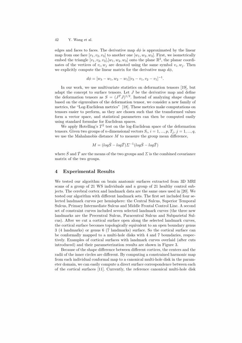
42 Y. Wang et al.
edges and faces to faces. The derivative map dφ is approximated by the linearmap from one face [v1, v2, v3] to another one [w1, w2, w3]. First, we isometricallyembed the triangle [v1, v2, v3],[w1, w2, w3] onto the plane R
2, the planar coordi-nates of the vertices of vi, wj are denoted using the same symbol vi, wj . Thenwe explicitly compute the linear matrix for the derivative map dφ,
dφ = [w3 − w1, w2 − w1][v3 − v1, v2 − v1]−1.
In our work, we use multivariate statistics on deformation tensors [19], butadapt the concept to surface tensors. Let J be the derivative map and definethe deformation tensors as S = (JT J)1/2. Instead of analyzing shape changebased on the eigenvalues of the deformation tensor, we consider a new family ofmetrics, the “Log-Euclidean metrics” [18]. These metrics make computations ontensors easier to perform, as they are chosen such that the transformed valuesform a vector space, and statistical parameters can then be computed easilyusing standard formulae for Euclidean spaces.
We apply Hotelling’s T 2 test on the log-Euclidean space of the deformationtensors. Given two groups of n-dimensional vectors Si, i = 1, ..., p, Tj , j = 1, ..., q,we use the Mahalanobis distance M to measure the group mean difference,
M = (logS − logT )Σ−1(logS − logT )
where S and T are the means of the two groups and Σ is the combined covariancematrix of the two groups.
4 Experimental Results
We tested our algorithm on brain anatomic surfaces extracted from 3D MRIscans of a group of 21 WS individuals and a group of 21 healthy control sub-jects. The cerebral cortex and landmark data are the same ones used in [20]. Wetested our algorithm with different landmark sets. The first set included four se-lected landmark curves per hemisphere: the Central Sulcus, Superior TemporalSulcus, Primary Intermediate Sulcus and Middle Frontal Control Line. A secondset of constraint curves included seven selected landmark curves (the three newlandmarks are the Precentral Sulcus, Paracentral Sulcus and Subparietal Sul-cus). After we cut a cortical surface open along the selected landmark curves,the cortical surface becomes topologically equivalent to an open boundary genus3 (4 landmarks) or genus 6 (7 landmarks) surface. So the cortical surface canbe conformally mapped to a multi-hole disks with 4 and 7 boundaries, respec-tively. Examples of cortical surfaces with landmark curves overlaid (after cutsintroduced) and their parameterization results are shown in Figure 3.
Because of the shape difference between different cortices, the centers and theradii of the inner circles are different. By computing a constrained harmonic mapfrom each individual conformal map to a canonical multi-hole disk in the param-eter domain, we can easily compute a direct surface correspondence between eachof the cortical surfaces [11]. Currently, the reference canonical multi-hole disk

Brain Mapping with the Ricci Flow 43
is arbitrarily chosen. For landmark curve matching, we guaranteed the match-ing of both curve ends. For other parts, we match curves based on unit speedparameterization on both curves.
Based on the surface matching results, the Jacobian matrices were computedas described in Section 3. For each point on the cortical surface, we ran permu-tation test with 5000 random assignments of subjects to groups to estimate thestatistical significance of the areas with group differences in surface morphom-etry. Figure 4 and 5 illustrates our experimental results. We compared left andright cortical surface morphology between 21 control subjects and 21 WS pa-tients with mappings constrained by a total of 4 and 7 selected landmark curves.Different sets of landmarks were used as anchors to evaluate the impact of thechoice of anatomical constraints on the results. The significance maps, for theleft and right hemispheres, show group differences at the voxel level, between WSpatients and control subjects. Mappings with 4 and 7 selected landmark curveswere computed. We detected few significant shape differences between left andright cortical surfaces (i.e., anatomical asymmetries) in both the control groupand the WS group. Even so, we did find significant shape differences for bothleft and right cortical surfaces between WS and control subjects. We also foundthe regions with differences detected at the voxel level were consistent for themappings computed with 4 and 7 selected landmark curves. However, detectionpower was not as high as expected in regions around the landmarks. Our futureresearch will examine the statistics in the vicinity of the chosen landmarks, andmultiple comparison correction methods, for example based on controlling thefalse discovery rate, will be used to assess the overall significance of the groupdifferences.
Fig. 3. Cortical surfaces with landmark curves and their conformal parameterizationresults. The first row shows a cortex with 4 landmarks and the second row shows acortex with 7 landmarks (one landmark is not visible in this view).
44 Y. Wang et al.
5 Conclusions and Future Work
We applied the Ricci flow conformal parameterization for brain cortical sur-face registration. Based on the derivative map between two matching surfaces,a multivariate statistic on the Jacobian matrices was used to study surface mor-phometry in WS. Experimental results suggest that the significantly differentareas were consistent with respect to the choice of landmark constraints and thealgorithm has the potential to detect systematic surface abnormalities associ-ated with disease. In the future, we will further study other possible statisticson the Jacobian matrices and find the optimal statistics for analyzing deforma-tions computed using our Ricci flow conformal parameterization-based surfacematching method. We will also validate our algorithm on larger databases ofanatomical models.
References
1. Fischl, B., Sereno, M.I., Tootell, R.B., Dale, A.M.: High-resolution inter-subjectaveraging and a coordinate system for the cortical surface. In: Human BrainMapping. Volume 8. (1999) 272–84
2. Bakircioglu, M., Joshi, S., Miller, M.: Landmark matching on brain surfaces vialarge deformation diffeomorphisms on the sphere. In: SPIE Medical Imaging. Vol-ume 3661. (1999) 710–15
3. Leow, A., Yu, C.L., Lee, S.J., Huang, S.C., Nicolson, R., Hayashi, K.M., Protas,H., Toga, A.W., Thompson, P.M.: Brain structural mapping using a novel hybridimplicit/explicit framework based on the level-set method. NeuroImage 24(3)(2005) 910–27
4. Thompson, P.M., Giedd, J.N., Woods, R.P., MacDonald, D., Evans, A.C., Toga,A.W.: Growth patterns in the developing human brain detected using continuum-mechanical tensor mapping. Nature 404(6774) (March 2000) 190–193
5. Davatzikos, C.: Spatial normalization of 3D brain images using deformable models.J. Comp. Assisted Tomography 20(4) (1996) 656–65
6. Durrleman, S., Pennec, X., Trouve, A., Thompson, P.M., Ayache, N.: Inferringbrain variability from diffeomorphic deformations of currents: An integrative ap-proach. Medical Image Analysis (2008) In Press.
7. Wang, Y., Chiang, M.C., Thompson, P.M.: Automated surface matching usingmutual information applied to riemann surface structures. In: Med. Image Comp.Comput.-Assist. Intervention, Proceedings, Part II. (Oct. 2005) 666–674
8. Pitiot, A., Delingette, H., Toga, A.W., Thompson, P.M.: Learning object corre-spondences with the observed transport shape measure. In: IPMI. (2003) 25–37
9. Davies, R.H., Twining, C.J., Cootes, T.F., Waterton, J.C., Taylor, C.J.: A min-imum description length approach to statistical shape modeling. In: IEEE TMI.Volume 21. (2002) 525–37
10. Thodberg, H.H.: Minimum description length shape and appearance models. In:IPMI. (2003) 51–62
11. Wang, Y., Gu, X., Chan, T.F., Thompson, P.M., Yau, S.T.: Brain surface conformalparameterization with the Ricci flow. In: IEEE ISBI. (2007) 1312–1315
12. Hurdal, M.K., Stephenson, K.: Cortical cartography using the discrete conformalapproach of circle packings. NeuroImage 23 (2004) S119–S128

Brain Mapping with the Ricci Flow 45
13. Angenent, S., Haker, S., Tannenbaum, A., Kikinis, R.: Conformal geometry andbrain flattening. Med. Image Comput. Comput.-Assist. Intervention (Sep. 1999)271–278
14. Gu, X., Wang, Y., Chan, T.F., Thompson, P.M., Yau, S.T.: Genus zero surfaceconformal mapping and its application to brain surface mapping. IEEE TMI 23(8)(Aug. 2004) 949–958
15. Wang, Y., Lui, L.M., Gu, X., Hayashi, K.M., Chan, T.F., Toga, A.W., Thompson,P.M., Yau, S.T.: Brain surface conformal parameterization using Riemann surfacestructure. IEEE TMI 26(6) (June 2007) 853–865
16. Commowick, O., Stefanescu, R., Fillard, P., Arsigny, V., Ayache, N., Pennec, X.,g. Malandain: Incorporating statistical measures of anatomical variability in atlas-to-subject registration for conformal brain radiotherapy. In: MICCAI. Volume II.,Palm Springs, CA, USA (2005) 927–934
17. Pennec, X., stefanescu, R., Arsigny, V., Fillard, P., Ayache, N.: Riemannian elastic-ity: A statistical regularization framework for non-linear registration. In: MICCAI.Volume II., Palm Springs, CA, USA (2005) 943–950
18. Arsigny, V., Fillard, P., Pennec, X., Ayache, N.: Log-Euclidean metrics for fast andsimple calculus on diffusion tensors”. In: Magn. Reson. Med. Volume 56. (2006)411–421
19. Lepore, N., Brun, C., Chou, Y.Y., Chiang, M.C., Dutton, R.A., Hayashi, K.M.,Luders, E., Lopez, O.L., Aizenstein, H.J., Toga, A.W., Becker, J.T., Thompson,P.M.: Generalized tensor-based morphometry of HIV/AIDS using multivariatestatistics on deformation tensors. IEEE TMI 27(1) (Jan. 2008) 129–141
20. Thompson, P.M., Lee, A.D., Dutton, R.A., Geaga, J.A., Hayashi, K.M., Eckert,M.A., Bellugi, U., Galaburda, A.M., Korenberg, J.R., Mills, D.L., Toga, A.W.,Reiss, A.L.: Abnormal cortical complexity and thickness profiles mapped inWilliams syndrome. J. Neurosciende (2005) 4146–4158
21. Guggenheimer, H.W.: Differential Geometry. Dover Publications (1977)22. Hamilton, R.S.: The Ricci flow on surfaces. Mathematics and general relativ-
ity (Santa Cruz, CA, 1986), Contemp. Math. Amer.Math.Soc. Providence, RI 71(1988)
23. Chow, B.: The Ricci flow on the 2-sphere. J. Differential Geom. 33(2) (1991)325–334
24. Thurston, W.P.: Geometry and Topology of Three-Manifolds. Princeton lecturenotes (1976)
25. Weitraub, S.H.: Differential Forms: A Complement to Vector Calculus. AcademicPress (2007)
26. Chow, B., Luo, F.: Combinatorial Ricci flows on surfaces. Journal DifferentialGeometry 63(1) (2003) 97–129

46 Y. Wang et al.
Fig. 4. Brain morphology study in 21 Williams Syndrome patients and 21 matchedcontrol subjects (intra group study).

Brain Mapping with the Ricci Flow 47
Fig. 5. Brain morphology study in 21 Williams Syndrome patients and 21 matchedcontrol subjects (inter group study).
Multi-Atlas Tensor-Based Morphometry and its
Application to a Genetic Study of 92 Twins
Natasha Lepore1, Caroline Brun1, Yi-Yu Chou1, Agatha D. Lee1, MarinaBarysheva1, Greig I. de Zubicaray2, Matthew Meredith2, Katie L. McMahon2,
Margaret J. Wright3, Arthur W. Toga1, and Paul M. Thompson1
1 Laboratory of Neuro Imaging, UCLA, Los Angeles, CA 90095, USA2 Centre for Magnetic Resonance, University of Queensland, Brisbane, Australia
3 Genetic Epidemiology Lab, Queensland Institute of Medical Research, Brisbane,Australia
Abstract. Here we develop a multi-template analysis for tensor-basedmorphometry (TBM) which aims to reduce error from the registrationstep. In conventional TBM, a single template is nonlinearly registered toall images in the study, and the deformation field statistics are computedfrom the transformations. Using an MRI dataset from 23 monozygoticand 23 dizygotic twin pairs, we instead registered each individual twinimage to 9 additional brain templates using a Riemannian fluid algo-rithm [3]. Average deformation tensors from multiple registrations werecomputed within each image, using a log-Euclidean framework [1]. Toquantify improvements as the number of registration templates increasedfrom 1 to 9, sequential t-tests assessed the significance of any error re-duction, as each new template was added. For each number of templates,we also computed two tensor-derived metrics, and maps of the intraclasscorrelation of local volume differences, to evaluate any power advantagesof multi-atlas TBM.
1 Introduction
Template selection is an important step in group analyses of brain MR images. Inparticular, in tensor-based morphometry (TBM), a set of images is non-linearlyregistered to a common reference image, and a statistical analysis is performedon the deformation tensors S =
√JT J , where J represents the Jacobian matrices
derived from the deformation fields.Detection power depends on several factors, and key among these is the qual-
ity of the non-linear registration, which also depends on the common target towhich all images are mapped. Typically, nonlinear registration is performed ei-ther to one of the controls, or to an average of them [8, 7, 13]. In theory theconstruction of a mean anatomical atlas can reduce the bias induced by regis-tering images to an individual control subject. In practice however, anatomicalboundaries and image gradients are often blurrier in the average image, whichmay reduce the accuracy of the registration. In [5] for instance, the ICBM53average brain was compared to a single individual template in a TBM study of
Multi-Atlas Tensor-Based Morphometry 49
HIV/AIDS patients. Greater effect sizes per voxel were found with the singletemplate when compared with those found using the ICBM53 brain as a regis-tration target. Even so, individual variability may cause a bias in the registrationwhen a single template is used, as the template may have a shape and inten-sity distribution that is closer to some subjects than to others. For instance, in[15], statistical power for TBM with single template registration was found todepend on which particular individual was selected as reference. Templates thatwere most average- in the sense of inducing the smallest deformation tensorswhen registered to other brains in the study- tended to generate more powerfulstatistics.
Our aim here was to design a new method that eliminates the dependence onindividual variability, while retaining the sharp features associated with registra-tion to a single target. One way to combine both of these requirements consistsof moving the averaging step until after the non-linear registration. The gist ofour averaging method consists of the following steps: starting from a set of brainMR images and a set of templates, we non-linearly register all images to all tem-plates individually. We then compute the deformation tensors for each imageas an average of those generated from the registration to individual templates.Other solutions to the template selection problem include ’targetless’ normaliza-tion as in [22], [19], [21], [10], and the selection of the optimal individual target[9, 15].
In the standard version of TBM [19, 2], statistics are performed on the de-terminants of the Jacobian matrices, detJ , or equivalently on the determinantsof the deformation tensors generated from the deformation field. In [14], mul-tivariate statistics were computed instead on the full deformation tensors. Asdeformation tensors do not form a vector space under standard matrix additionand scalar multiplication, computations were performed in the log-Euclideanframework [1]. Since statistics are computed on the deformation tensors or afunction of its components, for example the determinant, here we also performa log-Euclidean averaging on those tensors.
Our analysis was performed on a dataset of MR images from 23 monozygotic(MZ) and 23 dizygotic (DZ) twin pairs, as well as 10 template brain MR imagesfrom identically scanned healthy subjects who did not belong to those pairs.We used the intraclass correlation of the detJ as a statistic to characterize theinfluence of shared genes on local brain volume. Voxelwise permutation statisticswere computed to assess the significance of the results.
2 Method
2.1 Data
3D T1-weighted images were acquired from 23 pairs of monozygotic twins (MZ;20 males/26 females; 25.11.5SD years old) and 23 pairs of same-sex dizygotictwins (DZ; all same-sex pairs; 20 males/26 females; 23.52.2 years), as well as 10individuals of comparable age, scanned identically. All MR images were collected

50 N. Lepore et al.
using a 4 Tesla Bruker Medspec whole body scanner (Bruker Medical, Ettingen,Germany) at the Center for Magnetic Resonance (University of Queensland, Aus-tralia). Three-dimensional T1-weighted images were acquired with an inversionrecovery rapid gradient echo (MP-RAGE) sequence to resolve anatomy at highresolution. Acquisition parameters were as follows: inversion time (TI)/repetitiontime (TR)/echo time (TE) = 1500/2500/3.83 msec; flip angle =15 degrees; slicethickness = 0.9 mm, with an acquisition matrix of 256 x 256 x 256. The study wasapproved by the Institutional Review Boards at the University of Queenslandand at UCLA; all subjects gave informed consent.
Non-brain tissues were removed from all images using the Brain Surface Ex-traction tool (BSE) of BrainSuite [18]. The masked image was spatially normal-ized to the Colin27 standard brain by a 9-parameter (3 translations, 3 rotations,3 scales) transformation, using the FLIRT software [11].
2.2 Template averaging
Each individual image I was non-linearly registered to each of 9 templates usinga fluid (large-deformation) version of a Riemannian registration algorithm [3,17, 6], which guarantees diffeomorphic mappings. In order to compute averagesin a common space, all templates were also registered to a tenth template. Thedeformation fields resulting from the first registration step were concatenatedwith those of the second registration to obtain 9 sets of deformation fields in thecommon space for each image I. The deformation tensors S1(x, I) for the singletemplate case were then computed at each voxel x.
In the log-Euclidean framework, the deformation tensors are projected tothe tangent plane of the manifold on which they are defined, via their matrixlogarithm. Tensor addition is performed in this space and the result is projectedback to the original manifold. Thus, the n-templates average deformation tensorSn(x, I) at voxel x on image I is given by:
Sn(x, I) = exp1
nΣn
j=1 log S1j (x, I) (1)
2.3 Selecting the number of templates
Two measures were used to determine any improvements from increasing thenumber of templates. We describe both procedures in this section. Briefly, ourfirst comparison method consists of comparing the total magnitude of defor-mation tensors before and after the addition of a new template. In effect, thisamounts to determining how ’average’ the effective template would have to be togenerate the given set of deformation tensors. The second method we use beginswith the assumption that the registration error diminishes with the number oftemplates used. Thus we wish to compare the distance between the deformationtensors obtained from a given number of templates to that which would havebeen found had we had access to an infinite number of templates. In practice,we will use values found with 9 templates as our gold standard.
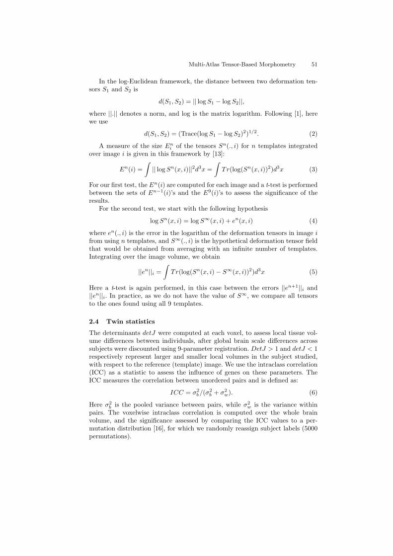
Multi-Atlas Tensor-Based Morphometry 51
In the log-Euclidean framework, the distance between two deformation ten-sors S1 and S2 is
d(S1, S2) = || log S1 − log S2||,
where ||.|| denotes a norm, and log is the matrix logarithm. Following [1], herewe use
d(S1, S2) = (Trace(log S1 − log S2)2)1/2. (2)
A measure of the size Eni of the tensors Sn(., i) for n templates integrated
over image i is given in this framework by [13]:
En(i) =
∫
|| log Sn(x, i)||2d3x =
∫
Tr(log(Sn(x, i))2)d3x (3)
For our first test, the En(i) are computed for each image and a t-test is performedbetween the sets of En−1(i)’s and the E9(i)’s to assess the significance of theresults.
For the second test, we start with the following hypothesis
log Sn(x, i) = log S∞(x, i) + en(x, i) (4)
where en(., i) is the error in the logarithm of the deformation tensors in image ifrom using n templates, and S∞(., i) is the hypothetical deformation tensor fieldthat would be obtained from averaging with an infinite number of templates.Integrating over the image volume, we obtain
||en||i =
∫
Tr(log(Sn(x, i) − S∞(x, i))2)d3x (5)
Here a t-test is again performed, in this case between the errors ||en+1||i and||en||i. In practice, as we do not have the value of S∞, we compare all tensorsto the ones found using all 9 templates.
2.4 Twin statistics
The determinants detJ were computed at each voxel, to assess local tissue vol-ume differences between individuals, after global brain scale differences acrosssubjects were discounted using 9-parameter registration. DetJ > 1 and detJ < 1respectively represent larger and smaller local volumes in the subject studied,with respect to the reference (template) image. We use the intraclass correlation(ICC) as a statistic to assess the influence of genes on these parameters. TheICC measures the correlation between unordered pairs and is defined as:
ICC = σ2b/(σ2
b + σ2w). (6)
Here σ2b is the pooled variance between pairs, while σ2
w is the variance withinpairs. The voxelwise intraclass correlation is computed over the whole brainvolume, and the significance assessed by comparing the ICC values to a per-mutation distribution [16], for which we randomly reassign subject labels (5000permutations).
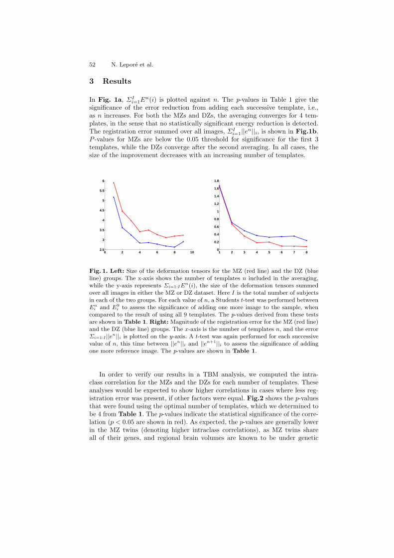
52 N. Lepore et al.
3 Results
In Fig. 1a, ΣIi=1E
n(i) is plotted against n. The p-values in Table 1 give thesignificance of the error reduction from adding each successive template, i.e.,as n increases. For both the MZs and DZs, the averaging converges for 4 tem-plates, in the sense that no statistically significant energy reduction is detected.The registration error summed over all images, ΣI
i=1||en||i, is shown in Fig.1b.
P -values for MZs are below the 0.05 threshold for significance for the first 3templates, while the DZs converge after the second averaging. In all cases, thesize of the improvement decreases with an increasing number of templates.
0 2 4 6 8 102.5
3
3.5
4
4.5
5
5.5
6
1 2 3 4 5 6 7 80
0.2
0.4
0.6
0.8
1
1.2
1.4
1.6
1.8
Fig. 1. Left: Size of the deformation tensors for the MZ (red line) and the DZ (blueline) groups. The x-axis shows the number of templates n included in the averaging,while the y-axis represents Σi=1:IEn(i), the size of the deformation tensors summedover all images in either the MZ or DZ dataset. Here I is the total number of subjectsin each of the two groups. For each value of n, a Students t-test was performed betweenEn
i and E9
i to assess the significance of adding one more image to the sample, whencompared to the result of using all 9 templates. The p-values derived from these testsare shown in Table 1. Right: Magnitude of the registration error for the MZ (red line)and the DZ (blue line) groups. The x-axis is the number of templates n, and the errorΣi=1:I ||e
n||i is plotted on the y-axis. A t-test was again performed for each successivevalue of n, this time between ||en||i and ||en+1||i to assess the significance of addingone more reference image. The p-values are shown in Table 1.
In order to verify our results in a TBM analysis, we computed the intra-class correlation for the MZs and the DZs for each number of templates. Theseanalyses would be expected to show higher correlations in cases where less reg-istration error was present, if other factors were equal. Fig.2 shows the p-valuesthat were found using the optimal number of templates, which we determined tobe 4 from Table 1. The p-values indicate the statistical significance of the corre-lation (p < 0.05 are shown in red). As expected, the p-values are generally lowerin the MZ twins (denoting higher intraclass correlations), as MZ twins shareall of their genes, and regional brain volumes are known to be under genetic
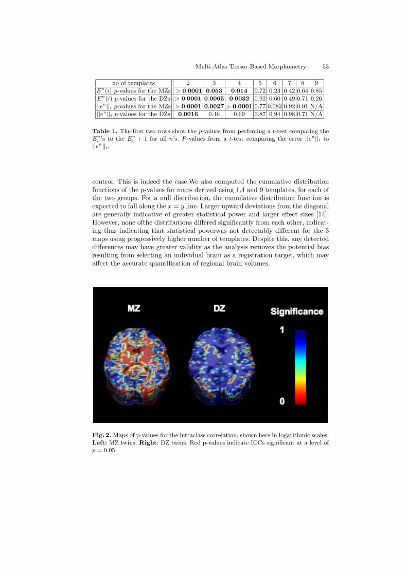
Multi-Atlas Tensor-Based Morphometry 53
no of templates 2 3 4 5 6 7 8 9
En(i) p-values for the MZs > 0.0001 0.053 0.014 0.72 0.23 0.42 0.64 0.85
En(i) p-values for the DZs > 0.0001 0.0065 0.0032 0.92 0.60 0.49 0.71 0.26
||en||i p-values for the MZs > 0.0001 0.0027 > 0.0001 0.77 0.082 0.92 0.91 N/A
||en||i p-values for the DZs 0.0016 0.46 0.69 0.87 0.94 0.98 0.71 N/A
Table 1. The first two rows show the p-values from perfoming a t-test comparing theEn
i ’s to the Eni + 1 for all n’s. P -values from a t-test comparing the error ||en||i to
||en||i.
control. This is indeed the case.We also computed the cumulative distributionfunctions of the p-values for maps derived using 1,4 and 9 templates, for each ofthe two groups. For a null distribution, the cumulative distribution function isexpected to fall along the x = y line. Larger upward deviations from the diagonalare generally indicative of greater statistical power and larger effect sizes [14].However, none ofthe distributions differed significantly from each other, indicat-ing thus indicating that statistical powerwas not detectably different for the 3maps using progressively higher number of templates. Despite this, any detecteddifferences may have greater validity as the analysis removes the potential biasresulting from selecting an individual brain as a registration target, which mayaffect the accurate quantification of regional brain volumes.
Fig. 2. Maps of p-values for the intraclass correlation, shown here in logarithmic scales.Left: MZ twins. Right: DZ twins. Red p-values indicate ICCs significant at a level ofp = 0.05.
54 N. Lepore et al.
4 Discussion
Here we presented a new multi-atlas version of Tensor-Based Morphometry. Alog-Euclidean averaging procedure was performed on the deformation tensorsgenerated from the multiple registrations, resulting in the reduction of regis-tration error and improved statistical power. At least for the case presentedhere, the error was significantly reduced up to an averaging of 4 templates. Fu-ture studies will assess how much multi-template TBM boosts power relative toother influential factors, including the sample sizes used, scan quality or fieldstrength, the regularization model and data fidelity term [5, 3], and the tensorstatistics used [14].
References
1. Arsigny V et al., Log-Euclidean metrics for fast and simple calculus on diffusion
tensors, Mag. Res. in Med. 56, (2006) 411–421.2. Ashburner J, A fast diffeomorphic image registration algorithm, Neuroimage 38,
(2007) 95–113.3. Brun C et al., Comparison of standard and Riemannian elasticity for Tensor-Based
Morphometry in HIV/AIDS, MICCAI workshop on Statistical Registration: Pair-wise and Group-wise Alignment and Atlas Formation (2007).
4. Chou YY et al., Automated Ventricular Mapping with Multi-Atlas Fluid Image
Alignment Reveals Genetic Effects in Alzheimer’s Disease, accepted for publicationin Neuroimage (2007).
5. Chiang MC et al., 3D pattern of brain atrophy in HIV/AIDS visualized using tensor-
based morphometry, Neuroimage 34, (2007) 44–60.6. Christensen GE et al., Deformable templates using large deformation kinematics,
IEEE-Trans. Imag. Process. 5, (1996) 1435–1447.7. Guimond et al. Average brain models: a convergence study, Comp. Vis. and Im.
Understanding 77, (1999) 192–210.8. Kochunov P et al., Regional spatial normalization: toward an optimal target, J.
Comp. Assist. Tomogr. 25, (2001) 805–816.9. Kochunov P et al. An optimized individual target brain in the Talairach coordinate
system, Neuroimage 17, (2003) 922–927.10. Kochunov P et al., Mapping structural differences of the corpus callosum in indi-
viduals with 18q deletions using targetless regional spatial normalization, Hum. BrainMap. 24, (2005) 325–331.
11. Jenkinson M and Smith S, A global optimisation method for robust affine registra-
tion of brain images, Med. Imag. Anal. 5, (2001) 143–56.12. Leow AD et al., Statistical properties of Jacobian maps and inverse-consistent de-
formations in non- linear image registration, IEEE-Trans. Med. Imag. 26, (2007)822-832
13. Lepore N et al., Mean template for Tensor-Based Morphometry using deformation
tensors, MICCAI (2007) 826–833.14. Lepore N et al., Multivariate statistics of the Jacobian matrices in Tensor-Based
Morphometry and their application to HIV/AIDS, IEEE-Trans. Med. Imag., in press(2008).
15. Lepore N et al., Best individual template selection from deformation tensor mini-
mization, ISBI (2008).

Multi-Atlas Tensor-Based Morphometry 55
16. Nichols TE, Holmes AP, Non parametric permutation tests for functional neu-
roimaging: a primer with examples, Hum. Brain Mapp. 15, (2001) 1–25.17. Pennec X et al., Riemannian elasticity: A statistical regularization framework for
non-linear registration, MICCAI, (2005) 943–950.18. Shattuck DW and Leahy RM, BrainSuite: an automated cortical surface identifi-
cation tool, Med. Imag. Anal. 8, (2002) 129–141.19. Studholme C et al., Deformation tensor morphometry of semantic dementia with
quantitative validation, Neuroimage 21, (2004) 1387-139820. Studholme C, Cardenas V, A template free approach to volumetric spatial normal-
ization of brain anatomy, Patt. Recogn. Lett. 25, (2004) 1191–1202.21. Twining CJ, A unified information-theoretic approach to groupwise non-rigid reg-
istration and model building MICCAI, (2005) 190–193.22. Thompson PM et al., Mathematical/Computational Challenges in Creating
Population-Based Brain Atlases, Hum. Brain Mapp. 9, (2000) 81–92.
Shape Registration with Spherical Cross
Correlation
Boris Gutman1,2 [email protected], Yalin Wang1,2, Tony Chan1, Paul M.Thompson2, and Arthur W. Toga2
1 UCLA Department of Mathematics2 UCLA Laboratory of Neuro Imaging
Abstract. We present a framework for shape alignment that generalizesseveral existing methods. We assume that the shape is a closed genus zerosurface. Our framework requires a diffeomorphic surface mapping to the2-sphere which preserves rotation. Our similarity measure is a globalspherical cross-correlation function of surface-intrinsic scalar attributes,weighted by the cross-correlation of the parameterization distortion. Thefinal similarity measure may be customized according to the surface-intrinsic scalar functions used in the application.
1 Introduction
Problems of shape alignment are ubiquitous in medical imaging. While manyproblem-specific solutions exist for particularly common cases (e.g. cortex, hip-pocampus) [1–3], high quality general shape alignment remains very much anopen problem. Our framework generalizes some existing methods without assum-ing the existence of any landmarks or data-specific features. We assume that theshape is a closed genus zero surface. Our framework requires a diffeomorphic sur-face mapping to the 2-sphere which preserves rotation. Our similarity measure isa global spherical cross-correlation function of surface-intrinsic scalar attributes,weighted by the cross-correlation of the parameterization distortion, sometimesknown as the conformal factor. The final similarity measure may be customizedaccording to the surface-intrinsic scalar functions used in the application. Higherorder scalar functions such as mean and Gaussian curvature may be used in con-junction with low order ones, like distance to mass center, to incorporate morelocalized shape information in addition to global measures.
In this study we have used a global conformal mapping as the sphericalparameterization, and only the distance to mass center as intrinsic scalar shapemeasure. Using our method, we created atlases and registered shapes from apopulation of hippocampi.
2 Previous work
There is doubtless a galaxy of existing general shape alignment methods, and dueto space limitations we will only mention those most prevalent and those closest
Shape Registration with Spherical Cross Correlation 57
to the present work. Davies [4] has used an information-theoretic framework toformulate shape alignment as a minimum description length (MDL) problem.Here, each point is treated as an independent variable, while the cost functionis aimed at reducing the ”code length” of each shape’s representation in thisshape space. The beauty of this statistical approach lies in its ability to registermultiple shapes simultaneously without the need to select a ”target” shape.Of course, this is also its limitation, as for example when a known atlas existsand all data shapes are to be registered to it. The method requires a sphericaldiffeomorphism like ours.
Variants of the well-known ICP algorithm are another variety of recent devel-opments in rigid shape alignment. Granger [5] introduced the EM-ICP method.ICP’s proclivity for terminating at suboptimal local minima is greatly reducedby treating the problem as a general expectation-maximization problem. A mul-tiscale approach is used: at coarser scales, the blurring factor is sufficient to givecrude but correct alignment, which is improved upon in later refined stages,where the algorithm approaches the original ICP. Though quite robust, themethod depends on the scale of blurring factor being set correctly to avoidlocal minima. Thus, avoiding them is not guaranteed. Our method, by contrast,performs a global search non-iteratively. Thus, a global maximum correlation isguaranteed irrespective of the shape’s original orientation without the need totune any parameters.
Much like our algorithm, some previous methods have used spherical harmon-ics for rigid shape alignment. Among them are the first order ellipsoid (FOE)method, popularized by Brechbuhler [6] and used extensively in medical imag-ing [7, 8] applications and SHREC, a recent variant of the ICP algorithm. Likeours, these methods make use of rotational properties of spherical harmonics.
FOE alignment uses the fact that a shape reconstructed from only the firstorder spherical harmonics forms an ellipsoid in object space. The method workswell when the ellipsoid’s three axes have distinct lengths, which largely dependson the shape itself and the degree to which the spherical parameterization pre-serves area. The method gives only a crude alignment and fails when two ormore axes have similar lengths. Even with a proper ellipsoid, there is a symme-try problem.
SHREC [9] is another variation of the ICP. As in our case, the correspon-dence search is done iteratively on the sphere via Euler’s rotation formula andicosahedral subdivision. The mapping satisfies our conditions, while the similar-ity measure is the RMSD. Since RMSD depends on the position of the objectin space, the algorithm requires an initial pre-alignment in both spaces. RigidQuaternion transform (RQT) is used to align shapes in R
3 after each iterationof parametric alignment. The main limitation of this algorithm is that it is notguaranteed to converge to the optimal solution (i.e. a correspondence which,when applied to RQT, minimizes RMSD). This is because the optimization inparameter space depends on the object’s position in native space. Thus, thoughthe search is more global than in the original ICP, the parameter space searchis still locally biased. The original ICP suffers the same problem.
58 B. Gutman et al.
The last algorithm uses a brute force correlation: it computes a cost functionanew for each rotation. To mitigate the cost of this, a hierarchical approach isused. Instead, we reduce parameter space alignment to a global refined search viathe FFT. Our numerical scheme separates the effects on computation time of thelevel of detail used for alignment and the number of rotation samples. In SHREC,these two are tied together owing to their brute-force nature. This means that wecan refine rotation space tessellation while maintaining the same level of surfacedetail without significantly affecting computation time. Our use of orientation-invariant shape attributes in conjunction with scale invariant cross-correlationmakes our approach completely independent of changes in object position andsize. SHREC, by contrast, requires volume normalization as a pre-processingstep.
3 Mathematical preliminaries
3.1 Spherical harmonics
Spherical harmonics are functions f : S2 → C which are simultaneously eigen-
functions of the Laplace-Beltrami and the angular momentum operators; theyare expressed explicitly as
Y ml (θ, φ) =
√
(2l + 1)(l − m)!
4(l + m)!Pm
l (cosθ)eimφ (1)
for degree and order m, l ∈ Z, |m| ≤ l , where Pml (x) is the associated Legendre
polynomial. Spherical harmonics form a countable orthonormal basis for square-integrable functions on the sphere. A projection of a function f ∈ L2(S
2) ontothis basis yields the SPH coefficients
f(l,m) =< f, Y ml > (2)
where < f, g > is the usual L2 inner product.A key property of spherical harmonics is their behavior under a shift on the
sphere. Given an element of the rotation group R ∈ SO(3), a rotated sphericalharmonic is expressed as
Y ml (ω) =
l∑
n=−l
Y nl (R−1ω)Dl
m,n(R) (3)
where
Dlm,n(R) = e−i(mα+nγ)dl
m,n(β), (4)
α, β, γ are the Euler angles of R and dlm,n are irreducible representations of
SO(3) [10],

Shape Registration with Spherical Cross Correlation 59
dlm,n(β) =
∑
t
(−1)t ×
√
(l + n)!(l − n)!(l + m)!(l − m)!
(l + n − t)!(l − m − t)!(t + m − n)!t!(5)
×(cosβ
2)2l+n−m−2t(sin
β
2)2t+m−n.
In particular, (3) implies that
f(ω) = g(R−1ω) =⇒ f(l,m) =
l∑
n=−l
g(l, n)Dlm,n(R). (6)
3.2 Discrete spherical cross correlation
Given two functions f, g ∈ L2(S2), their spherical cross-correlation is defined as
Cf,g(R) =
∫
S2
f(ω)g(R−1ω)dω. (7)
In the special case where f(ω) = g(R′−1ω), Cf,g(R) is maximized when R = R′,assuming that f is not spherically symmetric. For bandlimited functions, i.e. forthose functions whose spherical harmonic coefficients vanish for all l ≥ B forsome bandwidth B, the correlation becomes
Cf,g(R) =
B−1∑
l=0
l∑
m=−l
f(l,m)Λ(R)g(l,m). (8)
Here, Λ(R) is the operator associated with the rotation matrix. The expressionfor shifted spherical harmonic coefficients (6) implies that
Cf,g(R) =∑
l,m,n
f(l,m)g(l, n)Dlm,n(R). (9)
This expression forms the basis of our similarity measure.
3.3 Fast cross correlation via FFT
The material presented so far has been used in the prior works we mentioned.Now, we present a simple lemma which leads to a great speed up in computing thecorrelation (9). It suffices to make the observation that any rotation R(α, β, γ)may be expressed as a product of two rotations:
R(α, β, γ) = R1(α + π/2, π/2, 0)R2(β + π, π/2, γ + π/2). (10)
Now using the fact that
Dlm,n(R1 R2) =
∑
k
Dlm,k(R1)D
lk,n(R2), (11)
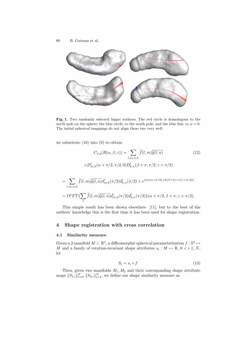
60 B. Gutman et al.
Fig. 1. Two randomly selected hippo surfaces. The red circle is homologous to thenorth pole on the sphere; the blue circle, to the south pole; and the blue line, to φ = 0.The initial spherical mappings do not align these two very well.
we substitute (10) into (9) to obtain
Cf,g(R(α, β, γ)) =∑
l,m,n,k
f(l,m)g(l, n) (12)
×Dlm,k(α + π/2, π/2, 0)Dl
k,n(β + π, π/2, γ + π/2)
=∑
l,m,n,k
f(l,m)g(l, n)dlm,k(π/2)dl
k,n(π/2) × ei(m(α+π/2)+k(β+π)+n(γ+π/2))
= IFFT∑
l
f(l,m)g(l, n)dlm,k(π/2)dl
k,n(π/2)(α + π/2, β + π, γ + π/2).
This simple result has been shown elsewhere [11], but to the best of theauthors’ knowledge this is the first time it has been used for shape registration.
4 Shape registration with cross correlation
4.1 Similarity measure
Given a 2-manifold M ⊂ R3, a diffeomorphic spherical parameterization f : S
2 7→M and a family of rotation-invariant shape attributes si : M 7→ R, 0 < i ≤ N ,let
Si = si f. (13)
Then, given two manifolds M1,M2 and their corresponding shape attributemaps S1,i
Ni=0, S2,i
Ni=1, we define our shape similarity measure as

Shape Registration with Spherical Cross Correlation 61
Fig. 2. Top surface from figure 1 is correlated to the bottom one, and its signalis shifted on the sphere without changing the shape’s position in object space. Thehomologous points now appear to be in good correspondence between the surfaces.
SM1,M2(R) = Cλ1,λ2
(R)N
∑
i=1
κiCS1,i,S2,i(R), (14)
where κi are user-defined shape attribute weights, and λ1, λ2 are spherical mapsof the conformal factor of each manifold. These last two are used to mitigatethe fact that scalar functions which appear similar on the sphere may in factrepresent vastly differently-sized regions on the original surfaces due to varyingarea distortion of the spherical map.
Because we recover shifts in object space with shifts on S2, we require that
the spherical parameterization preserve rotation in the following sense. SupposeM2 = R M1, and f1, f2 : S
2 7→ M1 ,M2 are spherical maps. Then
f2(ω) = R f1(R−1ω). (15)
Many existing parameterizations satisfy this requirement, e.g. [6, 12].
4.2 Previous methods as special cases
SHREC and FOE are special cases of our method. FOE simply takes the confor-mal factor λ to be constant and uses spherical harmonics up to order one only.This is equivalent to setting the bandwidth B to 2. The single shape attributeused is the Euclidian distance to the surface average value. This is roughly thesame as distance to mass center, especially for area-preserving spherical mapswith which FOE is typically used.
SHREC minimizes RMSD, which can be reduced to spherical cross-correlationsince 4πRMSD2
M1,M2(R) =
∑
i∈x,y,z
∫
S2
||S1,i − Λ(R)S2,i||2 (16)
=∑
i∈x,y,z
∫
S2
[S21,i + (Λ(R)S2,i)
2 − 2S1,iΛ(R)S2,i]
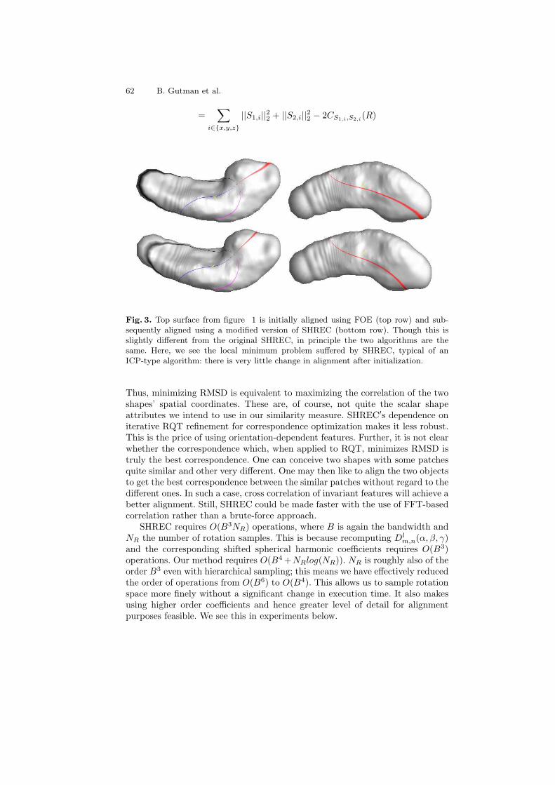
62 B. Gutman et al.
=∑
i∈x,y,z
||S1,i||22 + ||S2,i||
22 − 2CS1,i,S2,i
(R)
Fig. 3. Top surface from figure 1 is initially aligned using FOE (top row) and sub-sequently aligned using a modified version of SHREC (bottom row). Though this isslightly different from the original SHREC, in principle the two algorithms are thesame. Here, we see the local minimum problem suffered by SHREC, typical of anICP-type algorithm: there is very little change in alignment after initialization.
Thus, minimizing RMSD is equivalent to maximizing the correlation of the twoshapes’ spatial coordinates. These are, of course, not quite the scalar shapeattributes we intend to use in our similarity measure. SHREC′s dependence oniterative RQT refinement for correspondence optimization makes it less robust.This is the price of using orientation-dependent features. Further, it is not clearwhether the correspondence which, when applied to RQT, minimizes RMSD istruly the best correspondence. One can conceive two shapes with some patchesquite similar and other very different. One may then like to align the two objectsto get the best correspondence between the similar patches without regard to thedifferent ones. In such a case, cross correlation of invariant features will achieve abetter alignment. Still, SHREC could be made faster with the use of FFT-basedcorrelation rather than a brute-force approach.
SHREC requires O(B3NR) operations, where B is again the bandwidth andNR the number of rotation samples. This is because recomputing Dl
m,n(α, β, γ)and the corresponding shifted spherical harmonic coefficients requires O(B3)operations. Our method requires O(B4 +NRlog(NR)). NR is roughly also of theorder B3 even with hierarchical sampling; this means we have effectively reducedthe order of operations from O(B6) to O(B4). This allows us to sample rotationspace more finely without a significant change in execution time. It also makesusing higher order coefficients and hence greater level of detail for alignmentpurposes feasible. We see this in experiments below.
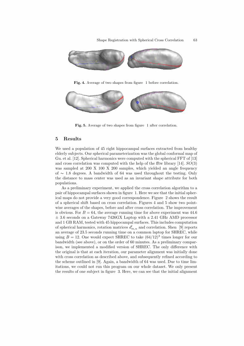
Shape Registration with Spherical Cross Correlation 63
Fig. 4. Average of two shapes from figure 1 before correlation.
Fig. 5. Average of two shapes from figure 1 after correlation.
5 Results
We used a population of 45 right hippocampal surfaces extracted from healthyelderly subjects. Our spherical parameterization was the global conformal map ofGu. et al. [12]. Spherical harmonics were computed with the spherical FFT of [13]and cross correlation was computed with the help of the fftw library [14]. SO(3)was sampled at 200 X 100 X 200 samples, which yielded an angle frequencyof ∼ 1.8 degrees. A bandwidth of 64 was used throughout the testing. Onlythe distance to mass center was used as an invariant shape attribute for bothpopulations.
As a preliminary experiment, we applied the cross correlation algorithm to apair of hippocampal surfaces shown in figure 1. Here we see that the initial spher-ical maps do not provide a very good correspondence. Figure 2 shows the resultof a spherical shift based on cross correlation. Figures 4 and 5 show two point-wise averages of the shapes, before and after cross correlation. The improvementis obvious. For B = 64, the average running time for above experiment was 44.6± 3.6 seconds on a Gateway 7426GX Laptop with a 2.41 GHz AMD processorand 1 GB RAM, tested with 45 hippocampal surfaces. This includes computationof spherical harmonics, rotation matrices dl
m,n and correlation. Shen [9] reportsan average of 23.5 seconds running time on a common laptop for SHREC, whileusing B = 12. One would expect SHREC to take (64/12)3 times longer for ourbandwidth (see above), or on the order of 60 minutes. As a preliminary compar-ison, we implemented a modified version of SHREC. The only difference withthe original is that at each iteration, our parameter alignment was initially donewith cross correlation as described above, and subsequently refined according tothe scheme outlined in [9]. Again, a bandwidth of 64 was used. Due to time lim-itations, we could not run this program on our whole dataset. We only presentthe results of one subject in figure 3. Here, we can see that the initial alignment
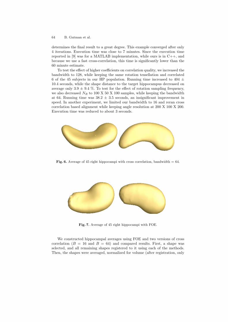
64 B. Gutman et al.
determines the final result to a great degree. This example converged after only4 iterations. Execution time was close to 7 minutes. Since the execution timereported in [9] was for a MATLAB implementation, while ours is in C++, andbecause we use a fast cross-correlation, this time is significantly lower than the60 minute estimate.
To test the effect of higher coefficients on correlation quality, we increased thebandwidth to 128, while keeping the same rotation tessellation and correlated6 of the 45 subjects in our HP population. Running time increased to 404 ±10.4 seconds, while the shape distance to the target hippocampus decreased onaverage only 3.9 ± 9.4 %. To test for the effect of rotation sampling frequency,we also decreased NR to 100 X 50 X 100 samples, while keeping the bandwidthat 64. Running time was 38.2 ± 3.5 seconds, an insignificant improvement inspeed. In another experiment, we limited our bandwidth to 16 and reran crosscorrelation based alignment while keeping angle resolution at 200 X 100 X 200.Execution time was reduced to about 3 seconds.
Fig. 6. Average of 45 right hippocampi with cross correlation, bandwidth = 64.
Fig. 7. Average of 45 right hippocampi with FOE.
We constructed hippocampal averages using FOE and two versions of crosscorrelation (B = 16 and B = 64) and compared results. First, a shape wasselected, and all remaining shapes registered to it using each of the methods.Then, the shapes were averaged, normalized for volume (after registration, only
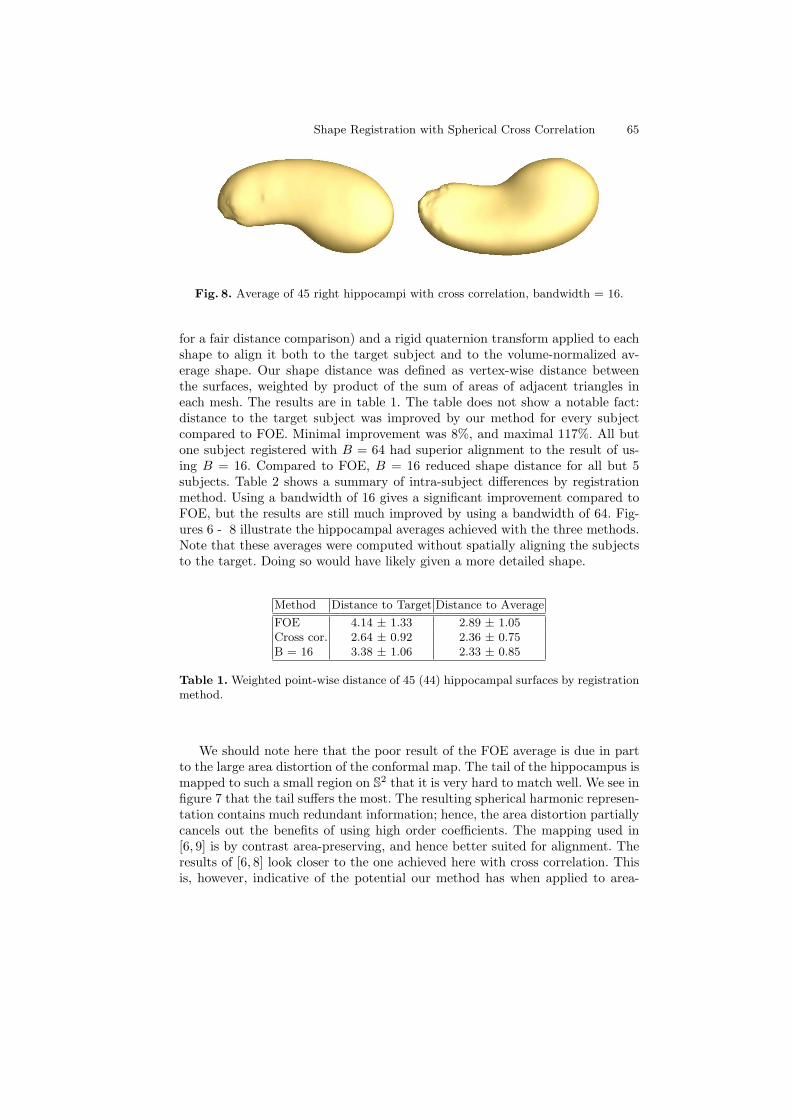
Shape Registration with Spherical Cross Correlation 65
Fig. 8. Average of 45 right hippocampi with cross correlation, bandwidth = 16.
for a fair distance comparison) and a rigid quaternion transform applied to eachshape to align it both to the target subject and to the volume-normalized av-erage shape. Our shape distance was defined as vertex-wise distance betweenthe surfaces, weighted by product of the sum of areas of adjacent triangles ineach mesh. The results are in table 1. The table does not show a notable fact:distance to the target subject was improved by our method for every subjectcompared to FOE. Minimal improvement was 8%, and maximal 117%. All butone subject registered with B = 64 had superior alignment to the result of us-ing B = 16. Compared to FOE, B = 16 reduced shape distance for all but 5subjects. Table 2 shows a summary of intra-subject differences by registrationmethod. Using a bandwidth of 16 gives a significant improvement compared toFOE, but the results are still much improved by using a bandwidth of 64. Fig-ures 6 - 8 illustrate the hippocampal averages achieved with the three methods.Note that these averages were computed without spatially aligning the subjectsto the target. Doing so would have likely given a more detailed shape.
Method Distance to Target Distance to Average
FOE 4.14 ± 1.33 2.89 ± 1.05Cross cor. 2.64 ± 0.92 2.36 ± 0.75B = 16 3.38 ± 1.06 2.33 ± 0.85
Table 1. Weighted point-wise distance of 45 (44) hippocampal surfaces by registrationmethod.
We should note here that the poor result of the FOE average is due in partto the large area distortion of the conformal map. The tail of the hippocampus ismapped to such a small region on S
2 that it is very hard to match well. We see infigure 7 that the tail suffers the most. The resulting spherical harmonic represen-tation contains much redundant information; hence, the area distortion partiallycancels out the benefits of using high order coefficients. The mapping used in[6, 9] is by contrast area-preserving, and hence better suited for alignment. Theresults of [6, 8] look closer to the one achieved here with cross correlation. Thisis, however, indicative of the potential our method has when applied to area-
66 B. Gutman et al.
preserving spherical maps, and we intend to experiment with this idea in theimmediate future.
common shape FOE vs. B = 64 FOE vs. B = 16 B = 16 vs. B = 64
target 61 % ± 26 % 25 % ± 23 % 30 % ± 18 %average 24 % ± 29 % 26 % ± 22 % -6 % ± 29 %
Table 2. Intra-subject improvement by registration method, in percentage of the sec-ond method’s result.
6 Conclusion
We have presented a framework for shape alignment which generalizes severalexisting methods. Our method is robust, fast and allows for use of greater detailin alignment than was possible before. The correspondence search is performedglobally and no pre-alignment is required; thus, the result and computation timeare independent of the shape’s size and initial orientation. Reaching a globalmaximum is always guaranteed. Our method can be tailored to suit a particularapplication by selecting the appropriate shape features for a particular data type.We intend to experiment with various shape attributes, apply area-preservingspherical maps to our method and extend the technique to automated patchselection and matching. Lastly, all software used here is available thorugh theLONI Pipeline environment. Please contact the authors for more details.
References
1. Shi, Y., Thompson, P., et al.: Direct mapping of hippocampal surfaces with intrinsicshape context. Neuroimage 37(3) (2007) 792–807
2. Tosun, D., Prince, J.: Cortical surface alignment using geometry driven multispec-tral optical flow. In: IPMI 2005. (2005)
3. Fischl, B., et al.: High-resolution intersubject averaging and a coordinate systemfor the cortical surface. Human Brain Mapping 8 (1999) 272–284
4. Davies, R., et al.: A minimum description length approach to statistical shapemodeling. IEEE Transactions on Medical Imaging 21(5) (2002) 525–537
5. Granger, S., Pennec, X.: Multi-scale em-icp: A fast and robust approach for surfaceregistration. In: Lecture Notes in Computer Science. (2002)
6. Brechbuhler, C., Gerig, G., Kubler, O.: Parameterization of closed surfaces for3d shape description. Computer Vision and Image Understanding 61(2) (1995)154–170
7. Gerig, G., Styner, M.: Shape versus size: Improved understanding of the morphol-ogy of brain structures. In: MICCAI 2001. (2001)
8. Gerig, G., Styner, M., et al.: Shape analysis of brain ventricles using spharm. In:IEEE Workshop on Mathematical Methods in Biomedical Image Analysis (MM-BIA’01). (2001)

Shape Registration with Spherical Cross Correlation 67
9. Shen, L., Huang, H., Makedon, F., Saykin, A.: Efficient registration of 3d spharmsurfaces. In: IEEE 4th Canadian Conference on Computer and Robot Vision.(2007)
10. Talman, J.: Special functions: A group-theoretic approach. W.A.Benjamin, Inc.(1968)
11. Sorgi, L., Daniilidis, K.: Template gradient matching in spherical images. ImageProcessing: Algorithms and Systems III. Proceedings of the SPIE 5298 (2004)88–98
12. Gu, X., Wang, Y., et al.: Genus zero surface conformal mapping and its applicationto brain surface mapping. IEEE Transactions on Medical Imaging 23(8) (2004)949
13. Healy, D., Rockmore, D., et al.: Ffts for the 2-sphere-improvements and variations.J. Fourier Anal. Applicat. 9(4) (2003) 341–385
14. Frigo, M.: A fast fourier transform compiler. In: ACM SIGPLAN Conference onProgramming Language Design and Implementation. (1999)
A Forward Model to Build Unbiased Atlases from
Curves and Surfaces
Stanley Durrleman1,2, Xavier Pennec1, Alain Trouvé2, and Nicholas Ayache1
1 INRIA - Asclepios Team-Project, Sophia Antipolis, France2 Centre de Mathématiques et Leurs Applications (CMLA), ENS-Cachan, France
Abstract. Building an atlas from a set of anatomical data relies on (1)the construction of a mean anatomy (called template or prototype) and(2) the estimation of the variations of this template within the popula-tion. To avoid biases introduced by separate processing, we jointly esti-mate the template and its deformation, based on a consistent statisticalmodel. We use here a forward model that considers data as noisy defor-mations of an unknown template. This diers from backward schemeswhich estimate a template by pulling back data into a common refer-ence frame. Once the atlas is built, the likelihood of a new observationdepends on the Jacobian of the deformations in the backward setting,whereas it is directly taken into account while building the atlas in theforward scheme. As a result, a specic numerical scheme is required tobuild atlases. The feasibility of the approach is shown by building atlasesfrom 34 sets of 70 sulcal lines and 32 sets of 10 deep brain structures.
1 Forward vs. Backward Models for Template Estimation
In the medical imaging eld, atlases are useful to drive the personalization ofgeneric models of the anatomy, to analyze the variability of an organ, to charac-terize and measure anatomical dierences between groups, etc. Many frameworkshave been proposed to build atlases from large database of medical images [14],much fewer were proposed for anatomical curves or surfaces [5, 6]. In any case,the underlying idea remains the same: one estimates a mean anatomy (calledtemplate) and one learns how this mean model deforms within a given popula-tion. The most widely used method in medical imaging is based on a backward
model that deforms every observations back to a common reference frame (SeeFig.1). However, we prefer here to base our statistical estimation on a forward
model, as pioneered in [7, 8], which considers the observations (Ti) as noisy de-formations (φi) of an unknown template (T ). Formally, the forward model canbe written as:
Ti = φi.T + εi (1.1)
whereas the backward model is:
φi.Ti = T + εi ⇐⇒ Ti = φ−1i T + φ−1
i εi (1.2)
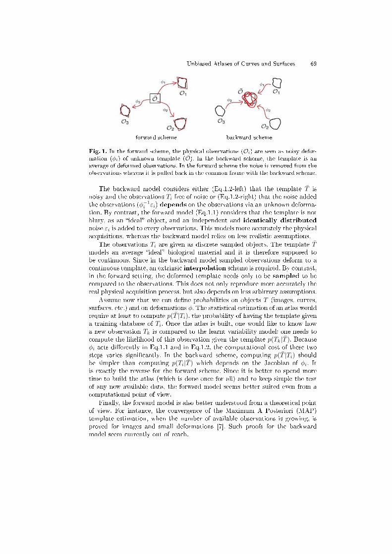
Unbiased Atlases of Curves and Surfaces 69
forward scheme backward scheme
Fig. 1. In the forward scheme, the physical observations (Oi) are seen as noisy defor-mation (φi) of unknown template (O). In the backward scheme, the template is anaverage of deformed observations. In the forward scheme the noise is removed from theobservations whereas it is pulled back in the common frame with the backward scheme.
The backward model considers either (Eq.1.2-left) that the template T isnoisy and the observations Ti free of noise or (Eq.1.2-right) that the noise addedthe observations (φ−1
i εi) depends on the observations via an unknown deforma-tion. By contrast, the forward model (Eq.1.1) considers that the template is notblury, as an ideal object, and an independent and identically distributed
noise εi is added to every observations. This models more accurately the physicalacquisitions, whereas the backward model relies on less realistic assumptions.
The observations Ti are given as discrete sampled objects. The template Tmodels an average ideal biological material and it is therefore supposed tobe continuous. Since in the backward model sampled observations deform to acontinuous template, an extrinsic interpolation scheme is required. By contrast,in the forward setting, the deformed template needs only to be sampled to becompared to the observations. This does not only reproduce more accurately thereal physical acquisition process, but also depends on less arbitrary assumptions.
Assume now that we can dene probabilities on objects T (images, curves,surfaces, etc.) and on deformations φ. The statistical estimation of an atlas wouldrequire at least to compute p(T |Ti), the probability of having the template givena training database of Ti. Once the atlas is built, one would like to know howa new observation Tk is compared to the learnt variability model: one needs tocompute the likelihood of this observation given the template p(Tk|T ). Becauseφi acts dierently in Eq.1.1 and in Eq.1.2, the computational cost of these twosteps varies signicantly. In the backward scheme, computing p(T |Ti) shouldbe simpler than computing p(Ti|T ) which depends on the Jacobian of φi. Itis exactly the reverse for the forward scheme. Since it is better to spend moretime to build the atlas (which is done once for all) and to keep simple the testof any new available data, the forward model seems better suited even from acomputational point of view.
Finally, the forward model is also better understood from a theoretical pointof view. For instance, the convergence of the Maximum A Posteriori (MAP)template estimation, when the number of available observations is growing, isproved for images and small deformations [7]. Such proofs for the backwardmodel seem currently out of reach.
70 S. Durrleman et al.
For all these reasons, we base here our statistical estimations on the forwardmodel. We show in this paper how the atlas building step, which is the mostcritical step in this paradigm, is possible in case of curves and surfaces. Com-pared to images, dealing with shapes requires specic numerical scheme. We takeadvantage here of a sparse deconvolution scheme we introduced recently [9, 10].
The paper is organized as follows. A general non parametric framework forshape statistics is introduced in Section 2. In Section 3 we detail the optimizationprocedure to estimate jointly a template and its deformations to the shapes. Asparse deconvolution method is presented to eectively compute the gradientdescent. In Section 4, we show templates computed from large sets of sulcal linesand sets of meshes of sub-cortical structures.
2 Non-parametric Representation of Shapes as Currents
As emphasized in [11, 12, 5], a current is a convenient way to model geometricalshapes such as curves and surfaces. The idea is to characterize shapes via vectorelds, which are used to probe them. A surface S is characterized by the ux ofany vector eld ω through it:
S(ω) =∫
S
ω(x).(u× v)(x)dσ(x) (2.1)
where u × v is the normal of the surface, (u, v) an orthonormal basis of itstangent plane) and dσ the Lebesgue measure on the surface. Similarly, a curveL is characterized by the path integral of any vector eld ω along it:
L(ω) =∫
L
ω(x).τ(x)dx (2.2)
where τ is the tangent of the curve. More generally, we dene a current T as alinear continuous mapping from a set of test vector elds W to R. This frameworkenables to dene addition, deformation, Gaussian noise on shapes, to measurea distance between shapes, without assuming point correspondences betweenobjects. We recall here some properties of currents to give a rigorous sense ofEq.1.1 in case of shapes. We refer the reader to [11, 13, 9] for more details.
As mappings from W to R, the currents build a vector space, denoted W ∗:(T1 + T2)(ω) = T1(ω) + T2(ω) and (λ.T )(ω) = λ.T (ω). For surfaces, this meansthat the ux through two surfaces is the sum of the ux through each surface: theaddition is equivalent to the union of surfaces. Scaling a surface means scalingthe power of the ux through the surface.
Suppose now that we can provide the test space W with a norm that measuresthe regularity of the vector elds. We can dene then a norm of a current Tas the maximum ux through T of any regular vector elds (i.e. ‖ω‖W ≤ 1):
‖T‖2W∗ = Sup‖ω‖W≤1 |T (ω)| (2.3)
The distance between two surfaces ‖S − S′‖W∗ is therefore obtained for theregular vector eld that best separates the two surfaces, in the sense that the

Unbiased Atlases of Curves and Surfaces 71
dierence of the ux through the two surfaces is the largest possible. This dis-
tance between shapes does not depend on how shapes are parametrized and does
not assume point correspondences between shapes.
For computational purposes, we suppose, from now onwards, that W is areproducible kernel Hilbert space (r.k.h.s) with kernel K [14]. In this setting,the space of currents is the dense span of all Dirac delta currents δα
x , which aredened by δα
x (ω) = 〈ω(x), α〉R3 for any ω ∈W . A Dirac current may be seen asa tangent (resp. normal) α entirely concentrated at point x. Although a curve(resp. a surface) has an innite number of tangents (resp. normals), a polygonallines (resp. a mesh) may be approximated in the space of currents by a nitesum
∑k δαk
xkwhere xk is the center of the segment (resp. center of the mesh cell)
and αk the tangent of the line (resp. the normal of the surface) at xk.Moreover, based on the Riesz theorem, we can show that for any current
T , the vector eld (within Eq. 2.3) that achieves Sup‖ω‖W≤1 |T (ω)| exists and is
unique. We denote this vector eld L−1W (T ) and call it the dual representation
of T . LW is isometric: it provides W ∗ with an inner product:
‖T‖2W∗ = 〈T, T 〉W∗ =⟨L−1
W (T ),L−1W (T )
⟩W
(2.4)
On Diracs we have:
L−1W (δα
x )(y) = K(y, x)α (2.5)
This equation shows that K is the Green kernel of LW . Applying Eq. 2.4 andEq. 2.5 leads to: ⟨
δαx , δβ
y
⟩W∗ = αtK(x, y)β (2.6)
This gives by linearity explicit and easily tractable formula to compute theinner product (and then the distance) between two shapes T =
∑i δαi
xiand
T ′ =∑
j δβjyj : 〈T, T ′〉W∗ =
∑i
∑j αt
iK(xi, yj)βj . The mapping L−1W is a sim-
ple convolution operator, as illustrated in Fig.2-a. On the contrary, nding thecurrent T whose associated vector eld γ is given (T = LW (γ)) is an ill-poseddeconvolution problem that requires specic numerical scheme as the one we willpresent in Section 3.3.
The kernel K enables also to dene an associated Gaussian noise on cur-rents ε. In innite dimension, ε maps every currents to a Gaussian variable suchthat Cov(ε(δα
x ), ε(δβy )) = αtK(x, y)β. If we set a grid Λ = xpp=1...N , the span
of (δxp)p∈Λ denes a nite dimensional space of currents. The corresponding ε isof the form
∑p∈Λ δ
αpxp where (αi) are centered Gaussian variables with covariance
matrix K−1 where K = (K(xi, xj))i,j∈Λ. In this last case, ε has a probability den-
sity function (pdf) which is proportionnal to exp(−‖ε‖2W∗). For our applicationswe will choose a Gaussian kernel: K(x, y) = exp(−‖x− y‖2 /λ2
W )Id.To make sense of the model Eq.1.1, one must still specify how this mod-
elling based on currents may be coupled with a deformation framework. If φis dieomorphism and S a surface, the ux of ω through the deformed shapeφ(S), denoted for general currents (φ] ? S)(ω), is equals to the ux through Sof the pulled-back vector eld φ] ? ω which is given by the change of variables

72 S. Durrleman et al.
formula within the ux integral. This enables to dene a general push-forwardaction of a dieomorphism on any currents. This action replaces for curvesand surfaces the usual action on images: (φ ? I)(x) = I(φ−1(x)). This is hereslightly more complex since we do not transport points but tangents or normals(dierential 1 and 2-forms to be even more precise). On the basis elements, thepush-forward action gives:
φ] ? δαx = δ
dxφ(α)φ(x) (2.7)
if α is a tangent of a curve and
φ] ? δu×vx = δ
dxφ(u)×dxφ(v)φ(x) (2.8)
if u×v is the normal of a surface. One notices that dxφ(u)×dxφ(v) = |dxφ| dxφ−t(u×v).
In the following, we restrict the deformations φ to belong to the group of dif-feomorphisms set up in [15, 16]: the dieomorphisms are obtained by integrationof a time-varying vector eld vt: ∂tφt = vt φt. The geodesic ows (φvt
t )t∈[0,1] arecompletely determined by the initial vector speed v0 which belongs to a r.k.h.s.V . The nal dieomorphism is denoted φv0 . How to nd such a dieomorphismthat best matches two sets of currents is explained in detail in [11, 13].
3 Joint Estimation of Template and Deformations
3.1 A Heuristic Maximum A Posteriori in Innite Dimension
From a Bayesian point of view, in Eq.1.1 (Ti = φi,] ? T + εi), Ti are the observa-tions, T is unknown, φi are hidden variables and εi independent and identicallydistributed Gaussian noise with known variance. Suppose now that we can de-ne Gaussian probability density functions (pdf) on the space of Currents W ∗
and on the space of initial vector elds V : pε(ε) = Cε exp(−‖ε‖2W∗ /σ2W ) and
pφ(v) = Cφ exp(−‖v‖2V /σ2V ). In that case, a Maximum A Posteriori (MAP) es-
timation for independent observations maximizes maxT
∏Ni p(Ti|T ). Formally,
p(Ti|T ) =∫
pε(Ti|T , vi0)pφ(vi
0)dv0 =∫
pε(Ti − φvi0
i T )pφ(vi0)dv0
Since the term within the integral depends on v0 by a geodesic shooting of dieo-morphisms, there are no closed forms for this likelihood. A usual approximationconsists in replacing the integral by the maximum of the distribution within the
integral (i.e. its rst mode). This leads to: p(Ti|T ) ∼ maxvi0pε(Ti − φ
vi0
i T )pφ(vi0)
which nally gives:
(T , φvi0) = argminT ,vi
0
N∑
i=1
1σ2
V
∥∥vi0
∥∥2
V+
1σ2
W
∥∥∥Ti − φvi0 .T∥∥∥2
W∗
(3.1)
called Fast Approximation with Mode (FAM). If we already dened Gaussianvariables in the space of currents (Section 2), such variables have no pdf because
Unbiased Atlases of Curves and Surfaces 73
W ∗ and V are of innite dimension. A more rigorous MAP derivation could bedone considering nite dimensional parametrization of the v0's and of the Ti's.For instance currents may be projected into a xed grid; but this would require toadapt the registration scheme of [11] to account for such a discretization. MarkovChain Monte Carlo (MCMC) approaches for sampling the posterior could be alsopossible along the lines of [17] but this is still challenging and out of the scopeof this paper.
3.2 A alternated Minimization Procedure
We solve Eq.3.1 by minimizing it alternatively with respect to the templateand to the deformations. When the template T is xed, each term of 3.1 can
be minimized separately. For a given observation Ti, minimizing 1σ2
V
∥∥vi0
∥∥2
V+
1σ2
W
∥∥∥Ti − φvi0
i .T∥∥∥2
W∗with respect to vi
0 is exactly a registration problem, as stated
and solved in [11, 13]. This step of the minimization consists therefore of Nregistrations of the template T to each observation Ti.
When the deformations φi are xed for every i = 1 . . . N , minimizing 3.1with respect to the template T leads to the minimization of:
J(T ) =12
N∑i=1
∥∥φ],i ? T − Ti
∥∥2
W∗ (3.2)
If all φi = Id (i.e. no deformation), the minimum is reached at the empirical
mean: T = 1N
∑Ni Ti. For arbitrary deformations, there is no closed form and
we use a gradient descent scheme. The gradient of Eq.3.2 is precisely:
∇T J =N∑
i=1
φ∗],i ? (φ],i ? T − Ti) (3.3)
where φ∗] is the adjoint action of φ]:⟨φ∗] ? T, T ′
⟩W∗
= 〈T, φ] ? T ′〉W∗ for any
currents T and T ′. This would be a matrix transpose if the action was linear. Inthis non-linear setting, standard computations give φ∗] ? T = LW (φ] ? L−1
W (T )).
With the backward scheme, Eq.3.2 would be: J(T ) = 12
∑Ni=1
∥∥T − φ],i ? Ti
∥∥2
W∗ ,
whose minimum has the closed form T = 1N
∑Ni=1 φ],i ? Ti. We see here why
the atlas building step is computationally more dicult in the forward setting.However, computing the likelihood of any new observations p(Ti|T ) will be muchsimpler and faster in this setting.
The input shapes Ti are sampled objects which are approximated as niteset of Dirac currents. As it will appear from this minimization procedure, thetemplate will also always remain a nite set of Dirac currents at every iteration.
Therefore, the current φ],i ? T − Ti is of the form∑
k δβi
k
yik
which nally leads to
φ]i ?L−1
W (φ],i ? T −Ti) =∑
k(dxφi)tK(φi(x), yik)βi
k in case of curves. Finally, the
74 S. Durrleman et al.
vector eld associated to the gradient of the energy 3.2 in case of curves can becomputed at any point x of the space:
L−1W (∇T J)(x) =
N∑i=1
(dxφi)t
(∑k
K(φi(x), yik)βi
k
)(3.4)
For surfaces, dxφti must be replaced by |dxφ| dxφ−1. At this stage, we see that the
gradient descent scheme could not be performed without an ecient numericalalgorithm to estimate the current ∇J whose associated vector eld is given byEq.3.4. The sparse deconvolution method of Section 3.3 precisely provides a niteset of Dirac current which approximates ∇J at any arbitrary accuracy, so thatthe template remains a nite set of Dirac currents at each iteration.
We initialize the algorithm by setting φi = Id, T = 1N
∑Ni=1 Ti and by com-
puting γT = L−1W (T ) via a Gaussian convolution. The current T is encoded as
a list of (position, vectors) that approximate small segments or small triangles.The dense vector eld γT is discretized at a xed grid's points: Λ = xp andtherefore encoded as an image of vectors. The following variable grad is also animage of vectors. We then iterate the following loop:
For i = 1 . . . N , φi ← registration of T to Ti. Until convergence do• grad = 0• For i = 1 . . . N do∗ transport tangents (normals) of T with φi (gives φ],i ? T ).
∗ store the (yik, βi
k) such that φ],i ? T − Ti =∑
k δβi
k
yik
∗ Deform Λ with φi and for each p ∈ Λ compute:· dxpφi by a nite dierence scheme· G =
∑k K(φi(xp), yi
k)βik (convolution)
· grad(p)← grad(p) + 2dxpφt
iG (or +2∣∣dxp
φi
∣∣ (dxpφi)−1G)
• γT ← γT − τgrad• Deconvolution of γT to give the new T (See section 3.3).
3.3 Sparse Deconvolution by a Matching Pursuit Algorithm
Like any linear combinations of the input currents, the mean current T isstored as the set of all weighted tangents (or normals) in the database T =(1/N)
∑N1 Ti =
∑n1 δαk
xkwhere n grows linearly with the number of observa-
tions. This heavy representation makes critical the registration of T right afterthe initialization step. But this representation is often far from being optimal:it may be highly redundant at the scale λW . To integrate this redundancy, wecompute the vector eld L−1
W (T ) (Fig.2-a) by convolution. Then, an adequatedeconvolution scheme could be applied to estimate an adapted basis on whichthe true solution T is decomposed in T =
∑k′ δ
αk′xk′ with fast decreasing terms.
The rst terms of this series will give therefore an approximation of T with anincreasing accuracy (Fig.2-b).
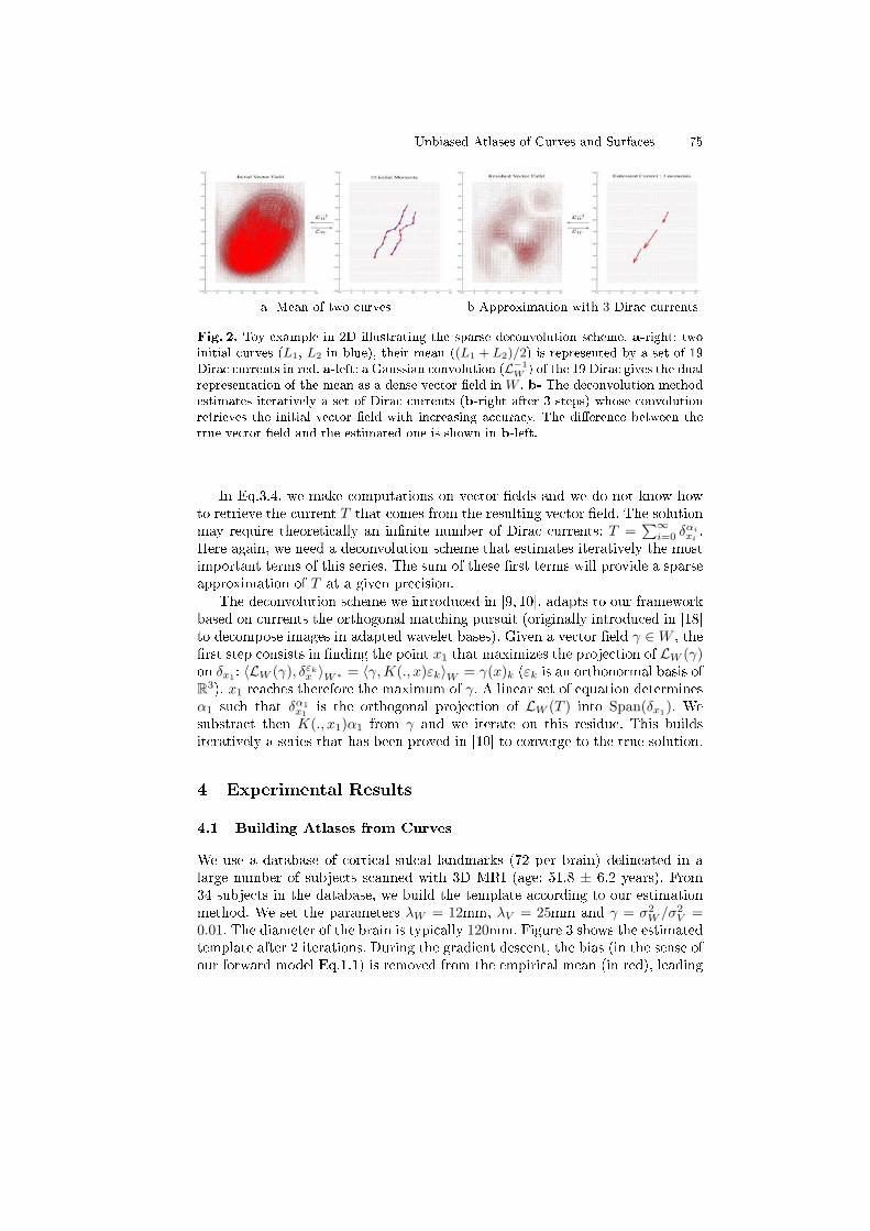
Unbiased Atlases of Curves and Surfaces 75
a- Mean of two curves b-Approximation with 3 Dirac currents
Fig. 2. Toy example in 2D illustrating the sparse deconvolution scheme. a-right: twoinitial curves (L1, L2 in blue), their mean ((L1 + L2)/2) is represented by a set of 19Dirac currents in red. a-left: a Gaussian convolution (L−1
W ) of the 19 Dirac gives the dualrepresentation of the mean as a dense vector eld in W . b- The deconvolution methodestimates iteratively a set of Dirac currents (b-right after 3 steps) whose convolutionretrieves the initial vector eld with increasing accuracy. The dierence between thetrue vector eld and the estimated one is shown in b-left.
In Eq.3.4, we make computations on vector elds and we do not know howto retrieve the current T that comes from the resulting vector eld. The solutionmay require theoretically an innite number of Dirac currents: T =
∑∞i=0 δαi
xi.
Here again, we need a deconvolution scheme that estimates iteratively the mostimportant terms of this series. The sum of these rst terms will provide a sparseapproximation of T at a given precision.
The deconvolution scheme we introduced in [9, 10], adapts to our frameworkbased on currents the orthogonal matching pursuit (originally introduced in [18]to decompose images in adapted wavelet bases). Given a vector eld γ ∈W , therst step consists in nding the point x1 that maximizes the projection of LW (γ)on δx1 : 〈LW (γ), δεk
x 〉W∗ = 〈γ, K(., x)εk〉W = γ(x)k (εk is an orthonormal basis ofR3). x1 reaches therefore the maximum of γ. A linear set of equation determinesα1 such that δα1
x1is the orthogonal projection of LW (T ) into Span(δx1). We
substract then K(., x1)α1 from γ and we iterate on this residue. This buildsiteratively a series that has been proved in [10] to converge to the true solution.
4 Experimental Results
4.1 Building Atlases from Curves
We use a database of cortical sulcal landmarks (72 per brain) delineated in alarge number of subjects scanned with 3D MRI (age: 51.8 ± 6.2 years). From34 subjects in the database, we build the template according to our estimationmethod. We set the parameters λW = 12mm, λV = 25mm and γ = σ2
W /σ2V =
0.01. The diameter of the brain is typically 120mm. Figure 3 shows the estimatedtemplate after 2 iterations. During the gradient descent, the bias (in the sense ofour forward model Eq.1.1) is removed from the empirical mean (in red), leading

76 S. Durrleman et al.
a- Sylvian Fissure (Left Hemisphere) b- All 70 sulci
Fig. 3. Estimated template from 34 subjects. Left: initial 34 Sylvian Fissure of the lefthemisphere (green), the empirical mean (red) and the estimated template (blue). Inblack, the mean lines computed from B-spline parametrization of curves [19]. Right:Same curves for 70 sulci. Although results look similar, only the template in blue isnot biased in the sense of the model Eq.1.1.
to an unbiased template (in blue). The sparse deconvolution scheme enables alsoto give a light representation of the template: whereas the database contains32643 segments (on average 960 segments per subject), the estimated templateis represented by only 1361 Dirac currents with an approximation error below5%. This would be of great interest in the future, for example to register thistemplate toward any new available data.
4.2 Building Atlases from Surfaces
We use a database of 10 segmented sub-cortical structures of the brain (Caudate,Putamen, Globus Pallidus, Amygdala and Hippocampus) in large number ofautistics and healthy children scanned with 3D MRI (age 2.7 ± 0.3) [20]. From25 autistics and 7 controls, we build the template according to our estimationmethod for surfaces. We use the parameters λW = 5mm, λV = 20mm, γ =σ2
W /σ2V = 0.001. The set of 10 sub-cortical structures have typically a diameter of
60mm. Figures 4-a,b show the estimated template after 2 iterations. Each Diraccurrent δα
x is represented by an equilateral triangle whose center of mass is x andnon-normalized normal α. Each of the 10 meshes has 2880 cells, so that the totalnumber of normals is 720e3. Thanks to the deconvolution scheme, the estimatedtemplate is represented by only 1344 normals with an approximation error below5%. In Fig.4-c, we show the dierence between the template of autistics andcontrols approximated by the proposed matching pursuit algorithm. Note thatthe anatomical dierences between both classes are not only captured by theirrespective templates but also by the main modes of the deformations φi.

Unbiased Atlases of Curves and Surfaces 77
a- Autistics b- Controls c- Dierence on hippocampus
Fig. 4. Estimated templates from 25 autistics (a) and 7 controls (b) for 10 sub-corticalstructures (one per color). In (c), the blue arrows approximate the dierence betweenautistics and controls' template, superimposed with the hippocampus of a control.
5 Conclusion and Perspectives
In this paper, we proposed a statistical model which estimates jointly a tem-plate, the deformations of the template to the observations and the noise onthese observations. This diers from methods that use extrinsic templates, thusintroducing a bias in the analysis of the variability. Our forward model considersobservations as noisy deformations of an unknown template. Compared to themore commonly used backward setting, this model requires a specic deconvolu-tion scheme to deal with the non-linear action of dieomorphisms on curves andsurfaces. However, once the model is built, we can decompose any new data intoa deformation of the template and a residual noise and then measure how likelythis decomposition may be with respect to the model. This oers a way to clas-sify data according to pathologies, to detect outliers in a database, to highlightwhere a given observation diers from a model, etc. Such a statistical inferencewould be more dicult within the backward framework since the likelihood ofany new observations would involve the Jacobian of the deformations that wetake here directly into account while building the atlas.
Numerical experiments show the feasibility and relevance of our approach. Inparticular, two templates were estimated from deep brain structures of autisticschildren and controls. The results suggest anatomical dierences between bothclasses. However, such results should be strengthen by rigorous statistical tests.Our future work will also evaluate the model with respect to its prediction andclassication capability.
Acknowledgments
We warmly thank Prof. Thompson (UCLA) for providing the sulcal lines databasethrough the Asclepios-LONI associated team BrainAtlas, as well as Prof. Gerig(University of Utah) for giving access to the database of deep brain structures.The work was partly supported by the European IP projet Health-e-Child (IST-2004-027749).
78 S. Durrleman et al.
References
1. Joshi, S., Davis, B., Jomier, M., Gerig, G.: Unbiased dieomorphic atlas construc-tion for computational anatomy. NeuroImage 23 (2004) 151160
2. Avants, B., Gee, J.: Geodesic estimation for large deformation anatomical shapeaveraging and interpolation. NeuroImage 23 (2004) 139150
3. Marsland, S., Twining, C.: Constructing dieomorphic representations for thegroupwise analysis of non-rigid registrations of medical images. Transactions onMedical Imaging 23(8) (2004) 10061020
4. Zollei, L., Learned-Miller, E., Grimson, E., Wells, W.: Ecient population regis-tration of data. In: Computer Vision for Biomedical Image Applications. Volume3765 of Lecture Notes in Computer Science., Springer (2005) 291301
5. Glaunès, J., Joshi, S.: Template estimation from unlabeled point set data and sur-faces for computational anatomy. In Pennec, X., Joshi, S., eds.: Proc. of the Inter-national Workshop on the Mathematical Foundations of Computational Anatomy(MFCA-2006). (2006)
6. Chui, H., Rangarajan, A., Zhang, J., Leonard, C.: Unsupervised learning of anatlas from unlabeled point-sets. IEEE Trans. on Pattern Analysis and MachineIntelligence 26(2) (2004) 160172
7. Allassonnière, S., Amit, Y., Trouvé, A.: Towards a coherent statistical frameworkfor dense deformable template estimation. Journal of the Royal Statistical SocietySeries B 69(1) (2007) 329
8. Ma, J., Miller, M., Trouvé, A., Younes, L.: Bayesian template estimation in com-putational anatomy. To appear in NeuroImage (2008)
9. Durrleman, S., Pennec, X., Trouvé, A., Ayache, N.: Sparse approximation of cur-rents for statistics on curves and surfaces. In: Proc. Medical Image Computing andComputer Assisted Intervention (MICCAI). (2008) In press.
10. Durrleman, S., Pennec, X., Trouvé, A., Ayache, N.: Sparse approximation of cur-rents for statistics on curves and surfaces. Research Report 6571, INRIA (06 2008)
11. Vaillant, M., Glaunès, J.: Surface matching via currents. In: Proceedings of Infor-mation Processing in Medical Imaging. Volume 3565 of Lecture Notes in ComputerScience., Springer (2005) 381392
12. Durrleman, S., Pennec, X., Trouvé, A., Ayache, N.: Measuring brain variability viasulcal lines registration: a dieomorphic approach. In: Proc. Medical Image Com-puting and Computer Assisted Intervention (MICCAI). Volume 4791 of LectureNotes in Computer Science., Springer (2007) 675682
13. Glaunès, J.: Transport par diéomorphismes de points, de mesures et de courantspour la comparaison de formes et l'anatomie numérique. PhD thesis, UniversitéParis 13, http://cis.jhu.edu/ joan/TheseGlaunes.pdf (2005)
14. Aronszajn, N.: Theory of reproducing kernels. Transactions of the AmericanMathematical Society (68) (1950) 337404
15. Trouvé, A.: Dieomorphisms groups and pattern matching in image analysis.International Journal of Computer Vision 28 (1998) 213221
16. Dupuis, P., Grenander, U., Miller, M.: Variational problems on ows of dieo-morphisms for image matching. Quaterly of Applied Mathematics 56(3) (1998)587600
17. Allassonnière, S., Kuhn, E., Trouvé, A.: Bayesian deformable models building viaa stochastic approximation algorithm: A convergence study. Bernouilli Journal(2008) In revision.

Unbiased Atlases of Curves and Surfaces 79
18. Pati, Y., Rezaifar, R., Krishnaprasad, P.: Orthogonal matching pursuit: recur-sive function approximation with applications to wavelet decomposition. In: Conf.Record of the 27th Asilomar Conference on Signals, Systems and Computers. Vol-ume 1. (November 1993) 4044
19. Fillard, P., Arsigny, V., Pennec, X., Hayashi, K., Thompson, P., Ayache, N.: Mea-suring brain variability by extrapolating sparse tensor elds measured on sulcallines. NeuroImage 34(2) (January 2007) 639650
20. Hazlett, H., Poe, M., Gerig, G., Smith, R., Provenzale, J., Ross, A., Gilmore, J.,Piven, J.: Magnetic resonance imaging and head circumference study of brain sizein autism. The Archives of General Psychiatry 62 (2005) 13661376

MAP Estimation of Statistical Deformable
Templates Via Nonlinear Mixed Effects Models :
Deterministic and Stochastic Approaches
Stephanie Allassonniere1, Estelle Kuhn2, and Alain Trouve3
1 Center for Imaging Science, Johns Hopkins University, USA,2 LAGA, University Paris 13, France,
3 CMLA, ENS Cachan, France,[email protected], [email protected], [email protected]. ⋆
Abstract. In [1], a new coherent statistical framework for estimatingstatistical deformable templates relevant to computational anatomy (CA)has been proposed. This paper addresses the problem of population av-erage and estimation of the underlying geometrical variability as a MAPcomputation problem for which deterministic and stochastic approxima-tion schemes have been proposed. We illustrate some of the numericalissues with handwritten digit and 2D medical images and apply the es-timated models to classification through maximum likelihood.
1 Introduction
For the last decade, we are witnessing impressive achievements and the emer-gence of elaborated registration theories [2–4] but the definition of a proper sta-tistical framework for designing and inferring stochastic deformable templates ina principled way is much less mature. Despite a seminal contribution [5] and thefact that deformable templates can be cast into the general Grenander’s PatternTheory [6], the down-to-earth and fundamental problem of computing popula-
tion averages in presence of unobserved warping variables has not received somuch attention from a more mathematical statistics perspective. More statisti-cally oriented methods are slowly emerging [7–9] based on penalized likelihoodor equivalently MDL approaches. Another line of research is to deal with theproblem of population average as an estimation issue of proper stochastic (i.e.generative) models for which consistency issues should be addressed. In thisdirection, nonlinear mixed effects models (NLMM) are common tools in bio-statistics and pharmacocinetic [10] to deal with both modelisation and inferenceof common population factors (fixed effects) and distributions of unobserved in-dividuals factors (random effects). An active realm of research has emerged inthe 90’s for designing efficient and consistent estimation algorithms. The impor-tation of such ideas even in the limited context of population average of greylevel images in CA is extremely appealing and challenging –both theoretically
⋆ We are thankful to Dr. Craig Stark for providing us with the medical data
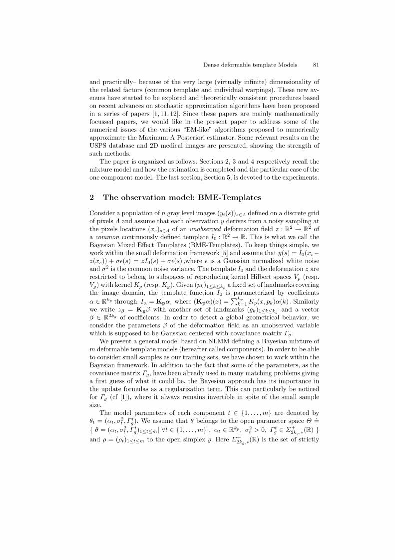
Dense deformable template Models 81
and practically– because of the very large (virtually infinite) dimensionality ofthe related factors (common template and individual warpings). These new av-enues have started to be explored and theoretically consistent procedures basedon recent advances on stochastic approximation algorithms have been proposedin a series of papers [1, 11, 12]. Since these papers are mainly mathematicallyfocussed papers, we would like in the present paper to address some of thenumerical issues of the various “EM-like” algorithms proposed to numericallyapproximate the Maximum A Posteriori estimator. Some relevant results on theUSPS database and 2D medical images are presented, showing the strength ofsuch methods.
The paper is organized as follows. Sections 2, 3 and 4 respectively recall themixture model and how the estimation is completed and the particular case of theone component model. The last section, Section 5, is devoted to the experiments.
2 The observation model: BME-Templates
Consider a population of n gray level images (yi(s))s∈Λ defined on a discrete gridof pixels Λ and assume that each observation y derives from a noisy sampling atthe pixels locations (xs)s∈Λ of an unobserved deformation field z : R
2 → R2 of
a common continuously defined template I0 : R2 → R. This is what we call the
Bayesian Mixed Effect Templates (BME-Templates). To keep things simple, wework within the small deformation framework [5] and assume that y(s) = I0(xs−z(xs)) + σǫ(s) = zI0(s) + σǫ(s) ,where ǫ is a Gaussian normalized white noiseand σ2 is the common noise variance. The template I0 and the deformation z arerestricted to belong to subspaces of reproducing kernel Hilbert spaces Vp (resp.Vg) with kernelKp (resp.Kg). Given (pk)1≤k≤kp
a fixed set of landmarks coveringthe image domain, the template function I0 is parameterized by coefficients
α ∈ Rkp through: Iα = Kpα, where (Kpα)(x) =
∑kp
k=1Kp(x, pk)α(k) . Similarlywe write zβ = Kgβ with another set of landmarks (gk)1≤k≤kg
and a vectorβ ∈ R
2kg of coefficients. In order to detect a global geometrical behavior, weconsider the parameters β of the deformation field as an unobserved variablewhich is supposed to be Gaussian centered with covariance matrix Γg.
We present a general model based on NLMM defining a Bayesian mixture ofm deformable template models (hereafter called components). In order to be ableto consider small samples as our training sets, we have chosen to work within theBayesian framework. In addition to the fact that some of the parameters, as thecovariance matrix Γg, have been already used in many matching problems givinga first guess of what it could be, the Bayesian approach has its importance inthe update formulas as a regularization term. This can particularly be noticedfor Γg (cf [1]), where it always remains invertible in spite of the small samplesize.
The model parameters of each component t ∈ 1, . . . ,m are denoted byθt = (αt, σ
2t , Γ
tg). We assume that θ belongs to the open parameter space Θ
.=
θ = (αt, σ2t , Γ
tg)1≤t≤m| ∀t ∈ 1, . . . ,m , αt ∈ R
kp , σ2t > 0, Γ t
g ∈ Σ+2kg,∗(R)
and ρ = (ρt)1≤t≤m to the open simplex . Here Σ+2kg,∗(R) is the set of strictly
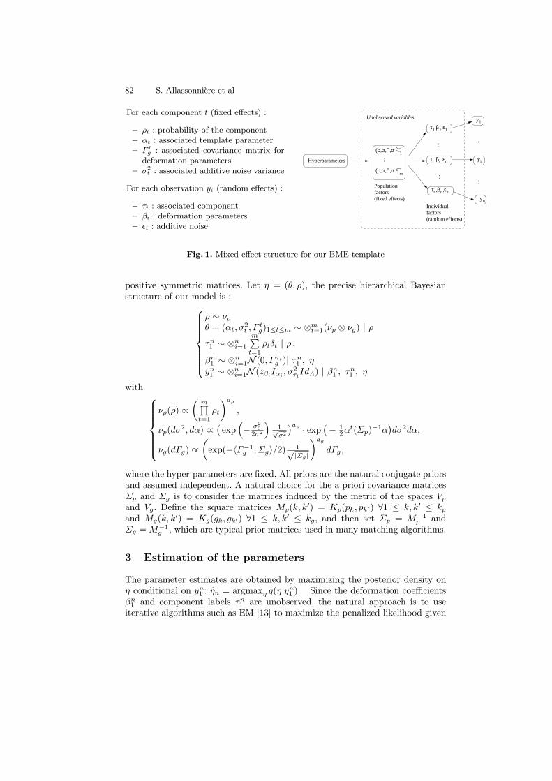
82 S. Allassonniere et al
For each component t (fixed effects) :
– ρt : probability of the component– αt : associated template parameter– Γ t
g : associated covariance matrix fordeformation parameters
– σ2
t : associated additive noise variance
For each observation yi (random effects) :
– τi : associated component– βi : deformation parameters– ǫi : additive noise
y1
yn
Populationfactors(fixed effects)
τ1,β1,ε1
Hyperparameters
Individualfactors(random effects)
τn,βn,εn
(ρ,α,Γ,σ 2)m
(ρ,α,Γ,σ 2)1
......
τι ,βι ,ει yi
Unobserved variables
......
......
Fig. 1. Mixed effect structure for our BME-template
positive symmetric matrices. Let η = (θ, ρ), the precise hierarchical Bayesianstructure of our model is :
ρ ∼ νρ
θ = (αt, σ2t , Γ
tg)1≤t≤m ∼ ⊗m
t=1(νp ⊗ νg) | ρ
τn1 ∼ ⊗n
i=1
m∑
t=1ρtδt | ρ ,
βn1 ∼ ⊗n
i=1N (0, Γ τig )| τn
1 , ηyn1 ∼ ⊗n
i=1N (zβiIαi
, σ2τiIdΛ) | βn
1 , τn1 , η
with
νρ(ρ) ∝
(
m∏
t=1ρt
)aρ
,
νp(dσ2, dα) ∝
(
exp(
−σ2
0
2σ2
)
1√
σ2
)ap· exp
(
− 12α
t(Σp)−1α
)
dσ2dα,
νg(dΓg) ∝
(
exp(−〈Γ−1g , Σg〉/2) 1√
|Σg|
)ag
dΓg,
where the hyper-parameters are fixed. All priors are the natural conjugate priorsand assumed independent. A natural choice for the a priori covariance matricesΣp and Σg is to consider the matrices induced by the metric of the spaces Vp
and Vg. Define the square matrices Mp(k, k′) = Kp(pk, pk′) ∀1 ≤ k, k′ ≤ kp
and Mg(k, k′) = Kg(gk, gk′) ∀1 ≤ k, k′ ≤ kg, and then set Σp = M−1
p andΣg = M−1
g , which are typical prior matrices used in many matching algorithms.
3 Estimation of the parameters
The parameter estimates are obtained by maximizing the posterior density onη conditional on yn
1 : ηn = argmaxη q(η|yn1 ). Since the deformation coefficients
βn1 and component labels τn
1 are unobserved, the natural approach is to useiterative algorithms such as EM [13] to maximize the penalized likelihood given
Dense deformable template Models 83
the observations yn1 . This likelihood is written as an integral over the hidden
variables, making the direct maximization a difficult task. The EM algorithmconsists in an iterative procedure to solve this problem. Each iteration of thealgorithm is divided into two steps; let l be the current iteration:
E Step: Compute the posterior law on (βn1 , τ
n1 ) as the following distribution:
νl(βn1 , τ
n1 ) ∝
n∏
i=1
q(yi|βi, ατi,l)q(βi|Γτi
g,l)ρτi,l
M Step: ηl+1 = argmaxη Eνl[log q(yn
1 , βn1 , τ
n1 , η)].
In the present context, we initialize the algorithm with the prior model η0.
3.1 Fast approximation with modes (FAM)
The expression in the M step requires the computation of the expectation withrespect to the posterior distribution of βn
1 , τn1 |y
n1 , computed in the E step, which
is known here up to the re-normalization constant. To overcome this obstacle,given an observation yi and a label t, the posterior distribution of the randomdeformation field is approximated at iteration l by a Dirac law on its mode β∗
l,i,t.This yields the following computation :
β∗
l,i,t = arg maxβ
log q(β|αt,l, σ2t,l, Γ
tg,l, yi)
= arg minβ
1
2βt(Γ t
g,l)−1β +
1
2σ2l,t
|yi −Kβp αt,l|
2
,
which is a standard template matching problem with the current parameters.We then approximate the joint posterior on (βi, τi) as a discrete distributionconcentrated at the m points (β∗
l,i,t)1≤t≤m with weights given by: wl,i(t) ∝
q(yi|β∗
l,i,t, αt,l)q(β∗
l,i,t|Γtg,l)ρt,l. The label τl,i is then sampled from the distribution
∑mt=1 wl,i(t)δt and the deformation is the mode of the drawn label βl,i = β∗
l,i,τi.
The maximization is then done on this approximation of the likelihood.
3.2 Using a stochastic version of the EM algorithm : SAEM-MCMC
An alternative to the computation of the E-step in a complex nonlinear con-text is to use the stochastic approximation EM algorithm (SAEM) [14] coupledwith an MCMC procedure [15] and a truncation on random boundaries. Ourmodel belongs to the exponential density family which means that: q(y, β, τ, η) =exp [−ψ(η) + 〈S(β, τ), φ(η)〉] , where the sufficient statistic S is a Borel functionon R
2kg × 1, . . . ,m taking its values in an open subset S of Rm and ψ, φ two
Borel functions on Θ× (the dependence on y is omitted for sake of simplicity).We introduce the following function: L : S×Θ×→ R as L(s; η) = −ψ(η)+
〈s, φ(η)〉 . Direct generalisation of the proof in [1] to the multicomponent model
84 S. Allassonniere et al
gives the existence of a critical function η : S → Θ × which satisfies: ∀η ∈Θ× ,∀s ∈ S, L(s; η(s)) ≥ L(s; η). Then, iteration l of this algorithm consists ofthe following four steps.
Simulation step: The missing data are drawn using a transition probabilityof a convergent Markov chain having the posterior distribution as stationarydistribution: (βl+1, τl+1) ∼ Πηl
((βl, τl), ·)Stochastic approximation step: Since the model is exponential, the stochas-
tic approximation is done on the sufficient statistics using the simulated values ofthe missing data: sl+1 = sl +∆l+1(S(βl+1, τl+1)−sl) ,where (∆l)l is a decreasingsequence of positive step-sizes.
Truncation step: A truncation is done on the stochastic approximation.Maximization step: The parameters are updated: ηl+1 = η(sl+1).
Concerning the choice of Πη used in the simulation step, as we aim tosimulate (βi, τi) through a transition kernel whose stationary distribution isq(β, τ |yi, η), we simulate τi with a kernel whose stationary distribution is q(τ |yi, η)and then βi through a transition kernel that has q(β|τ, yi, η) as stationary distri-bution. Given any initial deformation field ξ0 ∈ R
2kg , we run, for each componentt, Jl iterations of a hybrid Gibbs sampler (for each coordinate of the vector, aHasting-Metropolis sampling is done given the other coordinates) Πη,t usingthe conditional prior distribution βj |β−j as the proposal for the jth coordinate,β−j referring to β without its jth coordinate. So that we get Jl elements ξt,i =
(ξ(k)t,i )1≤k≤Jl
of an ergodic homogeneous Markov chain whose stationary distribu-tion is q(·|yi, t, η). Denoting ξi = (ξt,i)1≤t≤m, we simulate τi through the discrete
density with weights given by: qξi(t|yi, η) ∝
1
Jl
JlPk=1
ft(ξ
(k)
t,i)
q(yi,ξ(k)
t,i,t|η)
!−1
,where ft
is the density of the Gaussian distribution N (0, Γg,t). Then, we update βi by re-running Jl times the hybrid Gibbs sampler Πη,τi
starting from a random initialpoint β0. It has been proved in [12], that the sequence (ηl)l generated throughthis algorithm converges a.s. toward a critical point of the penalized likelihoodof the observations.
4 Single component model
We focus here on the single component model (m = 1). The unobserved vari-ables are only the deformation fields β and the parameters are reduced to θ =(α, σ2, Γg). In this particular setting, denoting by P the distribution governingthe observations and byΘ∗ = θ∗ ∈ Θ | EP (log q(y|θ∗)) = supθ∈Θ EP (log q(y|θ)),
it has been proved in [1] that the MAP estimator θn exists a.s. and convergestoward an element in Θ∗. From the algorithmical viewpoint, the FAM algorithmdoes not require any changes. Indeed, each E step only corresponds to a singlecomputation of the mode of the posterior density. However, the stochastic al-gorithm can be simplified. In the simulation step, only a single iteration of theMarkov chain (i.e. Jl = 1, ∀l) is needed for each iteration of the SAEM algo-rithm: βl+1 ∼ Πθl
(βl, ·) yielding a non homogeneous Markov chain. It has been

Dense deformable template Models 85
proved in [11], that the sequence (θl)l generated converges almost surely towarda critical point of the penalized likelihood of the observations.
5 Experiments
5.1 Estimation results
We illustrate this theoretical framework with the USPS handwritten digit databasewhich corresponds to non noisy gray level images. In addition, we compare thetwo algorithmical approaches on 2D medical images of the corpus calosum (thesplenium) and a part of the cerebellum.
Figure 2 shows the templates estimated from a training set (Figure 2-(a))of 20 or 40 images per digit with both algorithms for the models with oneand two components per class respectively. The results are quite similar, inparticular the two components present the same features for both algorithms.Topologically different shapes are separated (cf digits 7 and 2) and the otherdigit clusters are relevant. While estimating a single component, the templatesare good representatives of the shapes existing in the training set.
Concerning the geometrical variability, Figure 3, left image, presents somesynthetic examples drawn with respect to the model with the estimated param-eters. In spite of some artefacts described below, the kind of deformations learntapplied to the estimated templates looks like the elements of the training setwhich means that the algorithms capture this geometrical variability.
Last but not least, one could wonder how those algorithms deal with noisyimages. In [1], this particular case has been shown to fail with the FAM algo-rithm with a toy example. Whereas, in [11, 12], the authors have proved thetheoretical convergence of the two stochastic algorithms (for the mixture andsimple models). This supports the fact that the estimated parameters should beless sensitive to the noise that can appear in the data. This is what we showin Figure 1 for a database of 20 images per digit which is partly presented (a).The results are related to the theory. Indeed, the FAM algorithm is stuck in
(a) (b) (c) (d)
Fig. 2. (a) Some images of the USPS training set: 20 images per class. (b,c,d): Toprow : FAM Algorithm, Bottom row : SAEM-MCMC algorithm. (b): one componentprototype. (c-d): 2 component prototypes.
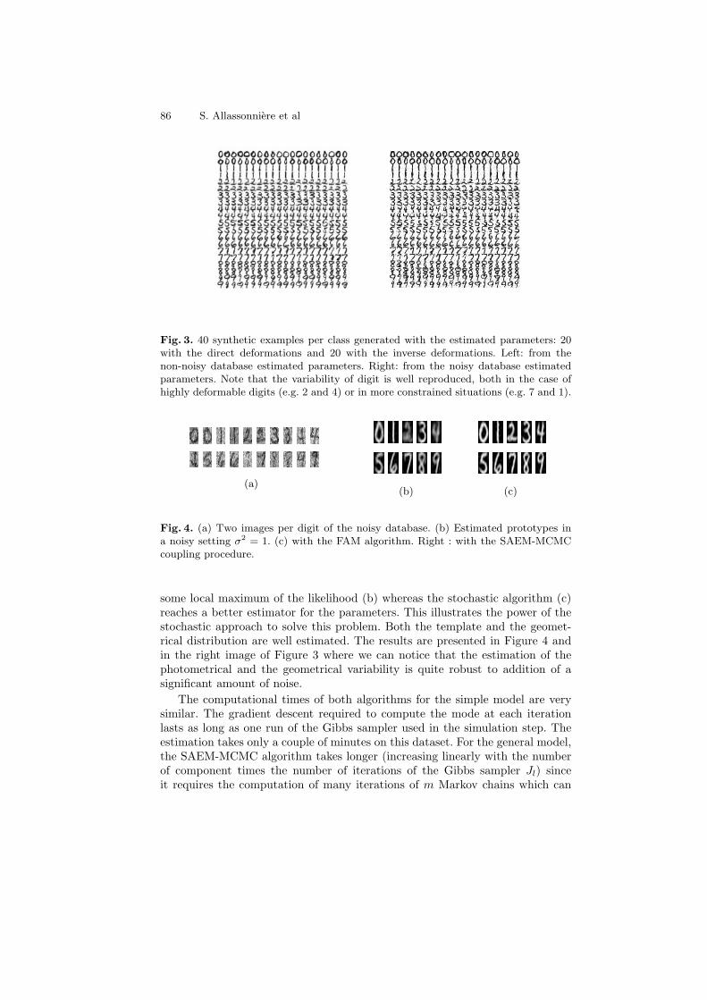
86 S. Allassonniere et al
Fig. 3. 40 synthetic examples per class generated with the estimated parameters: 20with the direct deformations and 20 with the inverse deformations. Left: from thenon-noisy database estimated parameters. Right: from the noisy database estimatedparameters. Note that the variability of digit is well reproduced, both in the case ofhighly deformable digits (e.g. 2 and 4) or in more constrained situations (e.g. 7 and 1).
(a)(b) (c)
Fig. 4. (a) Two images per digit of the noisy database. (b) Estimated prototypes ina noisy setting σ2 = 1. (c) with the FAM algorithm. Right : with the SAEM-MCMCcoupling procedure.
some local maximum of the likelihood (b) whereas the stochastic algorithm (c)reaches a better estimator for the parameters. This illustrates the power of thestochastic approach to solve this problem. Both the template and the geomet-rical distribution are well estimated. The results are presented in Figure 4 andin the right image of Figure 3 where we can notice that the estimation of thephotometrical and the geometrical variability is quite robust to addition of asignificant amount of noise.
The computational times of both algorithms for the simple model are verysimilar. The gradient descent required to compute the mode at each iterationlasts as long as one run of the Gibbs sampler used in the simulation step. Theestimation takes only a couple of minutes on this dataset. For the general model,the SAEM-MCMC algorithm takes longer (increasing linearly with the numberof component times the number of iterations of the Gibbs sampler Jl) sinceit requires the computation of many iterations of m Markov chains which can

Dense deformable template Models 87
(a) (b) (c) (d) (e)
(f) (g) (h)
Fig. 5. First row : Ten images of the training set representing the splenium and apart of the cerebellum. Second row : Results from the template estimation. (a) : graylevel mean image of the 47 images. Templates estimated (b) : with the FAM (c) : withthe stochastic algorithms on the simple model (d,e) : on the two component model.Third row : (f,g,h) : gray level mean image of the 47 images of the edges and estimatedtemplates with the FAM and the stochastic algorithm on the simple model.
actually be easily parallelized. In addition, the number Jl of iterations of theMarkov chain can be fixed all along the algorithm in the experiments.
We also test the algorithms on some medical images. The database we con-sider has 47 2D images, each of them representing the splenium (back of thecorpus calosum) and a part of the cerebellum. Some of the training images areshown in Figure (5) first row.
The results of the estimation are presented in Figure 5 where we can seethe improvement from the gray level mean (a) to our estimations. Image (b),corresponding to the deterministic algorithm result, shows a well contrasted sple-nium whereas the cerebellum remains a little bit blurry (note that it is still muchbetter that the simple mean). Image (c), corresponding to the stochastic EM al-gorithm result, presents some real improvement again. Indeed, the splenium isstill very contrasted, the background is not blurry and overall, the cerebellum iswell reconstructed with several branches. The two anatomical shapes are relevantrepresentants of the ones observed in the training set.
The estimation has been done while enabling the decomposition of the databaseinto two components. The two estimated templates (using the MCMC-SAEMalgorithm) are presented in Figure 5 (d) and (e). The differences can be seen inparticular on the shape of the splenium, where the fornix is more or less close tothe boundary of the image and the thickness of the splenium varies. The numberof branches in the two cerebella also tends to be different from one template tothe other (4 in the first component and 5 in the second one). The estimationsuffers from the small number of images we have. To be able to explain the huge
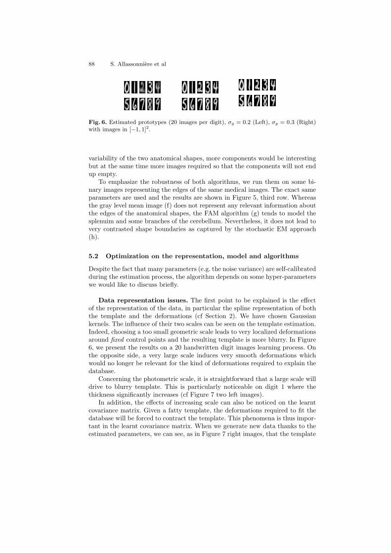
88 S. Allassonniere et al
Fig. 6. Estimated prototypes (20 images per digit), σg = 0.2 (Left), σg = 0.3 (Right)with images in [−1, 1]2.
variability of the two anatomical shapes, more components would be interestingbut at the same time more images required so that the components will not endup empty.
To emphasize the robustness of both algorithms, we run them on some bi-nary images representing the edges of the same medical images. The exact sameparameters are used and the results are shown in Figure 5, third row. Whereasthe gray level mean image (f) does not represent any relevant information aboutthe edges of the anatomical shapes, the FAM algorithm (g) tends to model thesplenuim and some branches of the cerebellum. Nevertheless, it does not lead tovery contrasted shape boundaries as captured by the stochastic EM approach(h).
5.2 Optimization on the representation, model and algorithms
Despite the fact that many parameters (e.g. the noise variance) are self-calibratedduring the estimation process, the algorithm depends on some hyper-parameterswe would like to discuss briefly.
Data representation issues. The first point to be explained is the effectof the representation of the data, in particular the spline representation of boththe template and the deformations (cf Section 2). We have chosen Gaussiankernels. The influence of their two scales can be seen on the template estimation.Indeed, choosing a too small geometric scale leads to very localized deformationsaround fixed control points and the resulting template is more blurry. In Figure6, we present the results on a 20 handwritten digit images learning process. Onthe opposite side, a very large scale induces very smooth deformations whichwould no longer be relevant for the kind of deformations required to explain thedatabase.
Concerning the photometric scale, it is straightforward that a large scale willdrive to blurry template. This is particularly noticeable on digit 1 where thethickness significantly increases (cf Figure 7 two left images).
In addition, the effects of increasing scale can also be noticed on the learntcovariance matrix. Given a fatty template, the deformations required to fit thedatabase will be forced to contract the template. This phenomena is thus impor-tant in the learnt covariance matrix. When we generate new data thanks to theestimated parameters, we can see, as in Figure 7 right images, that the template
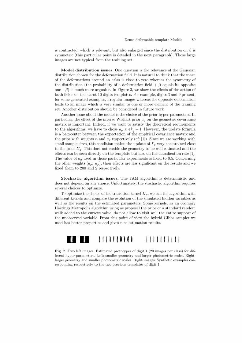
Dense deformable template Models 89
is contracted, which is relevant, but also enlarged since the distribution on β issymmetric (this particular point is detailed in the next paragraph). Those largeimages are not typical from the training set.
Model distribution issues. One question is the relevance of the Gaussiandistribution chosen for the deformation field. It is natural to think that the meanof the deformations around an atlas is close to zero whereas the symmetry ofthe distribution (the probability of a deformation field + β equals its oppositeone −β) is much more arguable. In Figure 3, we show the effects of the action ofboth fields on the learnt 10 digits templates. For example, digits 3 and 9 present,for some generated examples, irregular images whereas the opposite deformationleads to an image which is very similar to one or more element of the trainingset. Another distribution should be considered in future work.
Another issue about the model is the choice of the prior hyper-parameters. Inparticular, the effect of the inverse Wishart prior ag on the geometric covariancematrix is important. Indeed, if we want to satisfy the theoretical requirementsto the algorithms, we have to chose ag ≥ 4kg + 1. However, the update formulais a barycenter between the expectation of the empirical covariance matrix andthe prior with weights n and ag respectively (cf: [1]). Since we are working withsmall sample sizes, this condition makes the update of Γg very constrained closeto the prior Σg. This does not enable the geometry to be well estimated and theeffects can be seen directly on the template but also on the classification rate [1].The value of ag used in those particular experiments is fixed to 0.5. Concerningthe other weights (ap, aρ), their effects are less significant on the results and wefixed them to 200 and 2 respectively.
Stochastic algorithm issues. The FAM algorithm is deterministic anddoes not depend on any choice. Unfortunately, the stochastic algorithm requiresseveral choices to optimize.
To optimize the choice of the transition kernel Πη, we run the algorithm withdifferent kernels and compare the evolution of the simulated hidden variables aswell as the results on the estimated parameters. Some kernels, as an ordinaryHastings Metropolis algorithm using as proposal the prior or a standard randomwalk added to the current value, do not allow to visit well the entire support ofthe unobserved variable. From this point of view the hybrid Gibbs sampler weused has better properties and gives nice estimation results.
Fig. 7. Two left images: Estimated prototypes of digit 1 (20 images per class) for dif-ferent hyper-parameters. Left: smaller geometry and larger photometric scales. Right:larger geometry and smaller photometric scales. Right images: Synthetic examples cor-responding respectively to the two previous templates of digit 1.
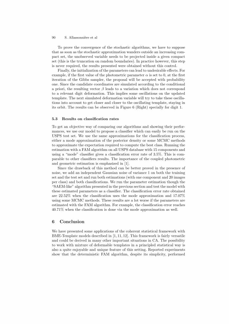
90 S. Allassonniere et al
To prove the convergence of the stochastic algorithms, we have to supposethat as soon as the stochastic approximation wanders outside an increasing com-pact set, the unobserved variable needs to be projected inside a given compactset (this is the truncation on random boundaries). In practice however, this stepis never required, the results presented were obtained without this control.
Finally, the initialization of the parameters can lead to undesirable effects. Forexample, if the first value of the photometric parameter α is set to 0, at the firstiteration of the Gibbs sampler, the proposal will be accepted with probabilityone. Since the candidate coordinates are simulated according to the conditionala priori, the resulting vector β leads to a variation which does not correspondto a relevant digit deformation. This implies some oscillations on the updatedtemplate. The next simulated deformation variable will try to take these oscilla-tions into account to get closer and closer to the oscillating template, staying inits orbit. The results can be observed in Figure 6 (Right) specially for digit 1.
5.3 Results on classification rates
To get an objective way of comparing our algorithms and showing their perfor-mances, we use our model to propose a classifier which can easily be run on theUSPS test set. We use the same approximations for the classification process,either a mode approximation of the posterior density or some MCMC methodsto approximate the expectation required to compute the best class. Running theestimation with a FAM algorithm on all USPS database with 15 components andusing a “mode” classifier gives a classification error rate of 3.5%. This is com-parable to other classifiers results. The importance of the coupled photometricand geometric estimation is emphasized in [1].
Since the drawback of this method can be better proved in the presence ofnoise, we add an independent Gaussian noise of variance 1 on both the trainingset and the test set and run both estimations (with one component and 20 imagesper class) and both classifications. We run the parameter estimation though the“SAEM-like” algorithm presented in the previous section and test the model withthese estimated parameters as a classifier. The classification error rate obtainedare 22.52% when the classification uses the mode approximation and 17.07%using some MCMC methods. These results are a lot worse if the parameters areestimated with the FAM algorithm. For example, the classification error reaches40.71% when the classification is done via the mode approximation as well.
6 Conclusion
We have presented some applications of the coherent statistical framework withBME-Template models described in [1, 11, 12]. This framework is fairly versatileand could be derived in many other important situations in CA. The possibilityto work with mixture of deformable templates in a principled statistical way isalso a quite enjoyable and unique feature of this setting. Reported experimentsshow that the deterministic FAM algorithm, despite its simplicity, performed
Dense deformable template Models 91
significantly worse especially under noisy conditions than the more sophisticatedstochastic alternative. The introduction of such MCMC methods are still quitechallenging in the 3D setting or for large deformation ([16] for a “FAM like”template estimation) but from an algorithmic point of view, there is a continuousinterpolation from deterministic to stochastic algorithms (just increasing thenumber of MCMC steps) so that there is no sharp complexity gaps betweento two approaches. Increasingly available computational power will make suchstochastic approaches more and more appealing in the future.
References
1. Allassonniere, S., Amit, Y., Trouve, A.: Toward a coherent statistical frameworkfor dense deformable template estimation. J.R.S.S. 69 (2007) 3–29
2. Toga, W.A., Thompson, P.M.: The role of image registration in brain mapping.Image and Vision Computing Journal 19(1–2) (2001) 3–24
3. Miller, M.I., Younes, L.: Group actions, homeomorphisms, and matching: A generalframework. Int. J. Comput. Vision 41(1-2) (2001) 61–84
4. Miller, M.I., Trouve, A., Younes, L.: Geodesic shooting for computational anatomy.J. Math. Imaging Vision 24 (2006) 209–228
5. Amit, Y., Grenander, U., Piccioni, M.: Structural image restoration through de-formable templates. JASA 86 (1991) 376–387
6. Grenander, U., Miller, M.: Pattern theory: from representation to inference. Ox-ford; New York: Oxford University Press (2007)
7. Glasbey, C.A., Mardia, K.V.: A penalised likelihood approach to image warping.Journal of the Royal Statistical Society, Series B 63 (2001) 465–492
8. Marsland, S., Twining, C.J., Taylor, C.J.: A minimum description length objectivefunction for groupewise non-rigid image registration. Im. Vis. Comp. (2007)
9. Van Leemput, K.: Probabilistic Brain Atlas Encoding Using Bayesian Inference.MICCAI 1 (2006) 704–711
10. Lindstrom, M., Bates, D.: Nonlinear mixed effects models for repeated measuresdata. Biometrics 46(3) (1990) 673–687
11. Allassonniere, S., Kuhn, E., Trouve, A.: Bayesian deformable models building viastochastic approximation algorithm: A convergence study. in revision
12. Allassonniere, S., Kuhn, E.: Stochastic algorithm for parameter estimation fordense deformable template mixture model. submitted
13. Dempster, A.P., Laird, N.M., Rubin, D.B.: Maximum likelihood from incompletedata via the EM algorithm. Journal of the Royal Statistical Society 1 (1977) 1–22
14. Delyon, B., Lavielle, M., Moulines, E.: Convergence of a stochastic approximationversion of the EM algorithm. Ann. Statist. 27(1) (1999) 94–128
15. Kuhn, E., Lavielle, M.: Coupling a stochastic approximation version of EM withan MCMC procedure. ESAIM Probab. Stat. 8 (2004) 115–131 (electronic)
16. Ma, J., Miller, M., Trouve, A., Younes, L.: Bayesian template estimation in com-putational anatomy. To appear in NeuroImage (2008)
Semiparametric estimation of rigidtransformations on compact Lie groups
Jeremie Bigot1, Jean-Michel Loubes1 and Myriam Vimond2
1 Institut de Mathematiques de Toulouse, Universite de Toulouse, 31062 ToulouseCedex 9, France,
2 Universite Haute Bretagne, Equipe de Statistique, Place du Recteur H. Le Moal,CS 24307, 35043 Rennes Cedex, France
Abstract. We study a simple model for the estimation of rigid trans-formations between noisy images. The transformations are supposed tobelong to a compact Lie group, and a new matching criteria based onthe Fourier transform is proposed. Consistency and asymptotic normal-ity of the resulting estimators are studied. Some simulations are used toillustrate the methodology, and we describe potential applications of thisapproach to various image registration problems.
1 Introduction
Originating in Grenander’s pattern theory, transformation Lie groups are com-monly used to model the deformations of images. The study of the propertiesand intrinsic geometries of such deformation groups is now an active field ofresearch (see e.g. [3], [10], [12], [13], [14], [18]). In this setting, an importantproblem is the estimation of the deformations that may exist between similarimages in the presence of additive noise. Rigid displacements such as transla-tions, rotations or affine transformations can be modeled by finite dimensionalLie groups. Hence, the estimation of rigid deformation parameters can be for-mulated as a semi-parametric estimation problem which is an important fieldof research in mathematical statistics [4]. Indeed, semiparametric modeling isconcerned with statistical problems where the parameters of interest are finitedimensional but where their observation is blurred by an infinite dimensionalparameter. Here, the finite-dimensional parameters are the Lie group elements,and the infinite-dimensional parameter is an unknown 2D or 3D image, which iswarped to obtain the different deformations. This image, that has to be recov-ered, is often called a template. The semiparametric framework provides optimalrecovery of the warping parameters, contrary to nonparametric methods, leadingto a better estimation of the template obtained by aligning the observed images.
As Lie groups are typically nonlinear spaces, an important question is thedevelopment of information geometry tools to extend classical notions such asasymptotic normality and efficiency, or the Cramer-Rao bound originally pro-posed for parameters lying in an Euclidean space. In the context of parametricstatistics, several generalizations of these concepts to arbitrary manifolds have
Shifts estimation on Lie groups 93
been proposed (see e.g. [17]). However, in the more general situation of semi-parametric models, there is not so much work dealing with the estimation ofparameters lying in a Lie group.
A first attempt in this direction has been proposed in [8], [20] for the simpleproblem of recovering shifts between one-dimensional noisy curves observed onan interval. The goal of this paper is extend such an approach to the moregeneral case where the shift parameters belong to a compact Lie group. Thanksto a general shift property of the Fourier transform on compact Lie groups, amatching criterion based on the Fourier transform of the data can be defined,and we study some statistical properties of the resulting estimators.
In Section 2, a simple model for shifts on groups is introduced. Some prop-erties on the Fourier transform are briefly reviewed (see [16] for further details),and are then used to define a general matching criterion on compact Lie groups.In Section 3, the consistency and the asymptotic normality of the estimators areestablished. Some numerical simulations are presented in Section 4, and exten-sions of the model are given in Section 5 for the registration of spherical images.Finally, we give some perspectives for future work. Note that the proofs of ourtheorems are based on the theory of M-estimation (see e.g. [19]), but are quitelong and technical, and are thus not given in this manuscript but can be foundin [2].
2 A shift model on Lie groups and a matching criteriabased on the Fourier transform
2.1 The Fourier transform on compact Lie groups
Let G be a compact Lie group. Denote by e the identity element, and by hg thebinary operation between two elements h, g ∈ G. Let L2(G) be the Hilbert spaceof complexed valued, square integrable functions on the group G with respect tothe Haar measure dg.
To define a Fourier transform on L2(G), a fundamental tool is the theory ofgroup representations, which aims at studying the properties of groups via theirrepresentations as linear transformation of vector spaces. More precisely, a rep-resentation is an homomorphism from the group G to the automorphism groupof a vector space. So let V be a finite-dimensional vector space, a representa-tion of G in V is thus defined as a continuous homomorphism π : G→ GL(V ),where GL(V ) denotes the set of automorphisms of V. Hence it provides a lineartransformation which depends on the vector space on which the group acts.
Every irreducible representation π of a compact group G in a vector space Vis finite dimensional, so we denote by dπ the dimension of V . By choosing a basisfor V , it is often convenient to identify π(g) with a matrix of size dπ × dπ withcomplex entries. The function g 7→ Trπ(g) is called the character of π. The char-acters carry the essential information about the group representation. Moreover,the fundamental theorem of Schur orthogonality states that the characters forman orthonormal system in L2(G) when π ranges over the dual set G of irreducible

94 J. Bigot et al.
and equivalent representations of G. In the case of compact groups, the dual Gis a countable set, and the Peter-Weyl Theorem states that the characters aredense in L2(G). Indeed, if π is a finite dimensional representation of G in thevector space V, then one can define, for every f ∈ L2(G), the linear mappingπ(f) : V → V by
π(f)v =∫
G
f(g)π(g)Tvdg, for v ∈ V.
The matrix π(f) is the generalization to the case of compact group of the usualnotion of Fourier coefficient. Then, Peter-Weyl Theorem implies that (for sim-plicity the same notation is used for π and its equivalence class in G)
f(g) =∑π∈G
dπTr (π(g)π(f)) and ‖f‖2L2(G) =∑π∈G
dπTr(π(f)π(f)
T)
(1)
In the sequel, we will also denote by 〈A,B〉HS = Tr (ATB) the Hilbert-Schmidt
inner product between two finite dimensional dπ × dπ matrices A and B.
2.2 A simple shift model on groups
Let X be a subset of Rd (with d = 2, 3 in our applications) and G be a compactLie group acting on X . A general deformation model for a set of J noisy signalswould be
Yj(x) = f∗(gj−1 · x) +Wj(x) for x ∈ X , (2)
where f∗ : X 7→ R is an unknown template, Wj(x) is some additive noise, andgj are the deformations to estimate. Our interest is to provide a very generalframework for image registration under warping effect given by model (2), andthus to deal with the general problem of estimation of the elements of a LieGroup G acting on a space X . In this paper, a simplest model for which X = Gis studied to give the main ideas of our approach. An example for which X 6= Gis given in Section 5 to show that our approach can be extended to more complexsituations, and we discuss possible extensions to more complex situations in theconcluding section.
Now, consider the following white noise model : for j = 1, . . . , J and g ∈ G
dYj(g) = fj(g)dg + εdWj(g), (3)
where fj(g) = f∗(h∗j−1g). The function f∗ : G → R is the unknown common
shape of the observed images Yj . The parameter h∗j , j = 1, . . . , J are the unknownshift parameters that we wish to estimate. Wj , j = 1, . . . , J are independentstandard Brownian sheets on the topological space G with measure dg, ε isan unknown noise level parameter which will tend to zero in our asymptoticconsiderations. Note that the white noise model (3) is a continuous model whichis a very useful tool for the theoretical study of statistical problem in imageanalysis. In practice, the noisy images Yj are typically discretely sampled on a
Shifts estimation on Lie groups 95
regular grid, but the model (3) can be shown to lead to comparable asymptotictheory in a sampled data model [5].
Obviously, without any further restriction on the set of possible shifts, themodel (3) is not identifiable. Indeed, if s is an element of G with s 6= e, thenone can replace the h∗j ’s in equation (3) by hj = h∗js and f∗ by f(g) = f∗(sg)without changing the formulation of the model. To ensure identification, wefurther assume that the set of parameters GJ is reduced to the subset A0 ⊂ Asuch that
A0 = (h1, . . . , hJ) ∈ A, h1 = e. (4)
This choice implies that the first image will be a reference and all the other im-ages will be warped onto this particular choice. Now, remark that since π(g)
T=
π(g−1), one has that π(fj) = π(f)π(h∗j−1) for all j = 1, . . . , J . This equality is
classically referred to as the shift property of the Fourier transform, and is at theheart of our estimation procedure to exhibit the shift parameters h∗j .
2.3 A matching criterion based on the Fourier transform
For h = (h1, . . . , hJ) ∈ A0, we propose to minimize the following criterion in-spired by recent results in [8] and [20] for the estimation of shifts between curves:
M(h1, . . . , hJ) =1J
J∑j=1
∥∥∥∥∥∥fj Thj− 1J
J∑j′=1
fj′ Thj′
∥∥∥∥∥∥2
L2(G)
, (5)
where Th : g ∈ G→ hg ∈ G. Using the Parseval-Plancherel formula, the criterionmay be rewritten in the Fourier domain as:
M(h) = M(h1, . . . , hJ) =1J
J∑j=1
∑π∈G
dπ
∥∥∥∥∥∥π(fj)π(hj)−1J
J∑j′=1
π(fj′)π(hj′)
∥∥∥∥∥∥2
HS
,
(6)for h = (h1, . . . , hJ) ∈ A0. Given that π(fj) = π(f∗)π(h∗j
−1), the criterion Mhas a minimum at h∗ = (h∗1, . . . , h
∗J) such that M(h∗) = 0.
2.4 The empirical criterion
Our estimation method is then based on the Fourier Transform of the noisy datagiven by model (3). Let π an irreducible representation of G into V . We considerthe following linear mappings from V to V which are defined from the model(3):
π(Yj) =∫
G
π(g−1)dYj(g) = π(fj) + επ(Wj), j = 1 . . . J,
where π(Wj) =∫
Gπ(g−1)dWj(g), j = 1 . . . J. Let us denote by (πkl(Wj)) the
matrix coefficients of π(Wj) : πkl(Wj) =∫
Gπkl(g−1)dWj(g). Using the Schur
96 J. Bigot et al.
orthogonality and the fact that Wj is a standard Brownian sheet on G, one ob-tains that the complex variables πkl(Wj) are independent identically distributedGaussian variables NC(0, d−1
π ).Let Gε be a finite subset of G such that the sequence Gε increases when ε
tends to 0 and ∪ε>0Gε = G. Practical choices for the set Gε will be discussedlater on for the case of Abelian groups and the non-commutative group SO(3).Then, we consider the following criterion:
Mε(h1, . . . , hJ) =1J
J∑j=1
∑π∈Gε
dπ
∥∥∥∥∥∥π(Yj)π(hj)−1J
J∑j′=1
π(Yj′)π(hj′),
∥∥∥∥∥∥2
HS
(7)
and our M-estimator is given by hε = arg minh∈A0 Mε(h).
3 Consistency and asymptotic normality of theM-estimator
Theorem 1. Assume that f∗ ∈ L2(G) is such that there does not exist a closedsubgroup H (except H = e or H = G) such that f(gh) = f(g) for all g ∈ G andh ∈ H. Moreover, suppose that for all π ∈ G such that π(f∗) is not identicallynull, then π(f∗) is invertible. Then, M has a unique minimum at h∗, and iflimε→0 ε
2∑
π∈Gεd2
π = 0, then hε converges in probability to h∗ = (h∗1, . . . , h∗J).
This Theorem shows the consistency of the estimators of the parameters h∗
when the noise level goes to zero (recall that in the discretized model, this isequivalent to the fact that the number of observations increase). We stress thatthis result is obtained by minimizing a quadratic contrast without prior knowl-edge of the main pattern, thanks to the empirical criterion (7) which enables toget rid of f∗. Asymptotic normality of these estimators and thus rates of con-vergence will provided in Theorem 2. The first condition of Theorem 1 ensuresidentifiability of the model since a function which would not satisfy this conditionwould be shift invariant, preventing any estimation. The second condition canbe viewed as a smoothness condition which ensures unicity of the minimizationscheme. In the following, we will denote by <(z) the real part of any complexnumber z.
As the estimator hε takes its values in a Lie group, it is not that obvious todefine a notion of asymptotic normality as the space A0 is typically not a linearspace if the group G is not Abelian. To overcome this, a classical approach is touse the exponential map to “project” hε into the Lie algebra G of G. If we canwrite hε = exp(uε), then one can study the asymptotic normality of uε which be-longs to the linear space G supposed to be of finite dimension p. For this, we firstre-express the criterion Mε defined on GJ as a function Mε defined on GJ . If G isa compact group, then the exponential map is surjective, but it is not necessarilyinjective. Hence, define U to be a compact neighborhood of 0 ∈ GJ onto which theexponential map is a smooth diffeomorphism, and let A = exp(U). For u ∈ UJ ,
Shifts estimation on Lie groups 97
we re-express our criterion as M(u1, . . . , uJ) = M(exp(u1), . . . , exp(uJ)), andMε(u1, . . . , uJ) = Mε(exp(u1), . . . , exp(uJ)). Then, define
uε = (u1, . . . , uJ) = arg minu∈U1
Mε(u1, . . . , uJ),
where U1 =(u1, . . . , uJ) ∈ UJ , u1 = 0
. Suppose that h∗1 = exp(u∗1), . . . , h
∗J =
exp(u∗J), with u∗ = (u1, . . . , uJ) ∈ UJ , then the following result holds:
Theorem 2. Assume that the conditions of Theorem 1 hold. Moreover, assumethat for all j = 2, . . . , J and k = 1, . . . , p
limε→0
ε∑
π∈Gε
d2π‖deπ
(du∗
jexp(xk)
)‖2HS = 0, (8)
and that
limε→0
supu1∈U
∑π∈G\Gε
dπ ‖π(f∗)‖2HS
∥∥deπ(du1 exp(xk1)
)∥∥2
HS
= 0 (9)
limε→0
supu1∈U
∑π∈G\Gε
dπ ‖π(f∗)‖2HS
∥∥∥∇xk2
u1deπ
(du1 exp(xk1)
)∥∥∥HS
= 0 (10)
limε→0
ε2 supu1∈U
∑π∈Gε
d2π
∥∥deπ(du1 exp(xk1)
)∥∥2
HS
= 0 (11)
limε→0
ε2 supu1∈U
∑π∈Gε
d2π
∥∥∥∇xk2
u1deπ
(du1 exp(xk1)
)∥∥∥HS
= 0, (12)
where x1, . . . , xp is an arbitrary basis of G. Then,
ε−1(uε − u∗) → N(0,H−1ΣH−1), as ε→ 0,
where Σ is a positive definite (J − 1)p × (J − 1)p matrix whose entries for2 ≤ j1, j2 ≤ J and 1 ≤ k1, k2 ≤ p are given by
Σ(j1,k1)×(j1,k1) =4J2
∑π∈G
dπ
(1− 1
J
)‖π(f∗)deπ
(du∗
j1exp(xk1)
)‖2HS
Σ(j1,k1)×(j1,k2) =4J2
∑π∈G
dπ
(1− 1
J
)<
⟨π(f∗)deπ
(du∗
j1exp(xk1)
), π(f∗)deπ
(du∗
j1exp(xk2)
)⟩HS
,
and for j1 6= j2 by
Σ(j1,k1)×(j2,k2) = − 4J2
∑π∈G
dπ1J<
⟨π(f∗)deπ
(du∗
j1exp(xk1)
), π(f∗)deπ
(du∗
j2exp(xk2)
)⟩HS
,
98 J. Bigot et al.
and where H is a positive definite (J − 1)p× (J − 1)p matrix whose entries for2 ≤ j1, j2 ≤ J and 1 ≤ k1, k2 ≤ p are given by
H(j1,k1)×(j1,k2) = − 2J
∑π∈G
dπ<⟨π(f∗)deπ
(du∗
j1exp(xk2)
)deπ
(du∗
j1exp(xk1)
)+ π(f∗)∇xk2
u∗j1deπ
(du∗
j1exp(xk1)
), π(f∗)
⟩HS
+1J
⟨π(f∗)deπ
(du∗
j1exp(xk1)
), π(f∗)deπ
(du∗
j1exp(xk2)
)⟩HS
,
and for j1 6= j2 by
H(j1,k1)×(j2,k2) = − 2J2
∑π∈G
dπ<⟨π(f∗)deπ
(du∗
j1exp(xk1)
), π(f∗)deπ
(du∗
j2exp(xk2)
)⟩HS
.
The convergence result in the above theorem must be understood for thevector uε = (u2, . . . , uJ) ∈ GJ−1 since the first component is fixed to u1 = 0.Moreover, the notation deπ stands for the differential of π at e, while du1 exp(xk1)corresponds to the differential of the exponential at u1 in the direction xk1 . Wepoint out that the estimator converges at the parametric rate of convergence, andthus optimal rate of convergence, which would not have been the case if we hadconsidered a preliminar estimate of f∗. This is one of the main achievementsof the semiparametric type methodology proposed in this paper. Proving theoptimality up to the constants imply studying the semiparametric efficiency ofthe estimators and falls beyond the scope of this paper. Some intuitions aboutsuch a result is provided in Section 6.
3.1 Abelian groups : the special case of the torus
The assumptions of Theorem 2 are rather technical and difficult to state in thevery general case. However, for Abelian groups their statement is much simpler,which is due to the fact that the mapping d expu : G → G reduces to the identityon G i.e. du exp(v) = v for all u ∈ G and v ∈ G. The assumptions can be rewrittenas
limε→0
ε2#Gε = 0, limε→0
ε∑
π∈Gε
|deπ(xk)|2 = 0, limε→0
∑π∈G\Gε
|π(f∗)|2∣∣deπ(xk)
∣∣2 = 0,
(13)where x1, . . . , xp is an arbitrary basis of G. Thus, Condition (??) states that thecommon shape is differentiable and its derivatives are square integrable on G.Conditions (13) give some assumptions on the choice of Gε.
As an illustrative example, let us consider the case where G = (R/Z)p whichcorresponds to the classical multi-dimensional Fourier decomposition of a func-tion f ∈ L2([0, 1]p)
f(x) =∑`∈Zp
c`(f)e`(x), for x = (x1, . . . , xp) ∈ [0, 1]d and ` = x = (`1, . . . , `p) ∈ Zd,
Shifts estimation on Lie groups 99
where e`(x) = π(x) = e−i2π(Pp
k=1 `kxk) and c`(x) = π(f) =∫[0,1]d
f(x)e`(x)dx.
Note that also that deπ(xk) = −i2π`k. Now, take Gε = (`1, . . . , `p) ∈ Zp, |`k| ≤`ε for all k = 1, . . . , p, for some positive integer `ε. Then, the following corollaryholds:
Corollary 1. Let G = (R/Z)p and f∗ ∈ L2([0, 1]p) be a periodic function sat-isfying the conditions of Theorem 1. Assume that h∗ ∈ GJ or equivalently thatu∗ ∈ ([0, 1]p)J . If
ε`p+2ε = o(1) and
∑(`1,...,`p)∈Zp
(|`1|2 + . . .+ |`p|2
)|c`(f∗)|2 <∞,
then ε−1(uε − u∗) → N(0, Γ−1), as ε→ 0, where the matrix Γ is given by
Γ(j1,k1)×(j1,k2) =∑`∈Z
(1− 1
J
)|c`(f∗)|2(2π)2`k1`k2 ,
Γ(j1,k1)×(j2,k2) = − 1J
∑`∈Z
|c`(f∗)|2(2π)2`k1`k2 for j1 6= j2,
4 Numerical simulations and some illustrative examples
4.1 A general gradient descent algorithm
To compute the estimator hε one has to minimize the functionMε(h). As this cri-terion is defined on a Lie group, a direct numerical optimization is generally notfeasible. Finding minima of functions defined on a Lie group is generally done byreformulating the problem as an optimization problem on its Lie algebra. Sincethe expression of the gradient of Mε(u) is available in a closed form, the follow-ing gradient descent algorithm with an adaptive step can be easily implemented:
Initialization : let u0 = 0 ∈ GJ , γ0 = 1‖∇u0Mε‖
, M(0) = Mε(u0), and setm = 0.Step 2 : let unew = um − γm∇umMε and M(m+ 1) = Mε(unew)
While M(m+ 1) > M(m) doγm = γm/κ, and unew = um − γm∇umMε, and M(m+ 1) = Mε(unew)End while
Then, take um+1 = unew and set m = m+ 1.Step 3 : if M(m) −M(m + 1) ≥ ρ(M(1) −M(m + 1)) then return to Step 2,else stop the iterations, and take hε = exp(um+1).
In the above algorithm, ρ > 0 is a small stopping parameter and κ > 1 is aparameter to control the choice of the adaptive step γm. Note that to satisfy theidentifiability constraints the first p components of um are held fixed to zero ateach iteration m.
100 J. Bigot et al.
4.2 Registration of translated 2D images
As an illustrative example, we consider the registration of translated 2D images(see [9] for a related work in a similar setting for 2D images). The chosen templatef∗ is the Shepp-Logan phantom image [1] of size N×N with N = 100 (see Figure1). Noisy images can be generated by translating this image and adding Gaussiannoise to each pixel value:
Y j(i1, i2) = f∗(i1N−h1
j ,i2N−h2
j )+σzj(i1, i2), 1 ≤ i1, i2 ≤ N, j = 1, . . . , J (14)
where i1, i2 denotes a pixel position in the image, zj(i1, i2) ∼i.i.d. N(0, 1), σ isthe level of noise, and h1
j , h2j ∈ [0, 1] are the unknown translation parameters
to estimate. One could argue that the sampled data model (14) does not trulycorrespond to the white noise model (3). However, as previously explained thereexists a correspondence between these two models in the sense that they areasymptotically equivalent if ε = σ
N (see [5]).We have repeated M = 100 simulations with J = 6 noisy images simulated
from the model (14). The various values taken for the translation parametersare the bold numbers given in Table 1. A typical example of a simulation runis shown in Figure 1. Here, G = [0, 1] × [0, 1] and its Lie algebra is G = R2.The criterion Mε(u) can be easily implemented via the use of the fast Fouriertransform for 2D images:
Mε(u) =1J
J∑j=1
∑|`1|≤`ε
∑|`2|≤`ε
∣∣∣∣∣∣yj`1,`2
ei2π(`1uj1+`2uj
2) − 1J
J∑j′=1
yj′
`1,`2ei2π(`1uj′
1 +`2uj′2 )
∣∣∣∣∣∣2
for u = (u11, u
21, . . . , u
1J , u
2J), and where the yj
`1,`2’s are the empirical Fourier co-
efficients of the image Y j . Moreover, if (x11, x
21, . . . , x
1J , x
2J) denotes the canonical
basis of the product space (R2)J , then the components of the gradient of Mε(u)are given by
∂
∂xkj
Mε(u) = − 2J
∑|`1|≤`ε
∑|`2|≤`ε
<
(i2π`k)yj`1,`2
ei2π(`1uj1+`2uj
2)(1J
J∑j′=1
yj′
`1,`2ei2π(`1uj′
1 +`2uj′2 ))
.
According to Corollary 1, the smoothing parameter `ε should be chosen suchthat ε`4ε = o(1). Since the models (14) and (3) are asymptotically equivalent ifε = σ
N , this condition becomes `ε = `N = o(N1/4). With N = 100, this suggeststo take `N ≤ 1001/4 ≈ 3.16. In Table 1 we give the empirical average of theestimated parameters over the M = 100 simulations, for the choice `N = 3,together with their standard deviation. The results are extremely satisfactoryas averages are very close to the true values and standard deviations are verysmall.
Shifts estimation on Lie groups 101
Fig. 1. A typical simulation run for J = 6 images generated from the model (14).
Table 1. Average and standard deviation (in brackets) of the estimators hj = (h1j , h
2j )
over M = 100 simulations. The bold numbers represent the true values of the param-eters (h1
j , h2j ).
j = 2 j = 3 j = 4 j = 5 j = 6
h1j 0.07 0.1 0.05 -0.05 -0.08
h1j 0.0704 (0.0031) 0.0997 (0.0031) 0.0494 (0.0028) -0.0502 (0.0031) -0.0801 (0.0032)
h2j 0.02 0.08 -0.10 -0.05 0.06
h2j 0.0201 (0.0031) 0.0803 (0.0031) -0.1002 (0.0030) -0.0493 (0.0029) 0.0604 (0.0032)
5 Registration of spherical images
In many applications, data can be organized as spherical images i.e. as functionsdefined on the unit sphere S2. For instance, spherical images are widely usedin robotics since the sphere is a domain where perspective projection can bemapped, and an important question is the estimation of the camera rotationfrom such images (see [11]). Obviously such data do not correspond exactlyto the shift model on group (3) as spherical images are defined on S2 whilethe shifts parameters belong the special orthogonal group SO(3). However thissetting corresponds to the general model (2) with X = S2 and G = SO(3), and amatching criterion similar to the one defined in equation (6) can still be definedby combining the spherical harmonics on S2 with the irreducible representationsof SO(3).
Indeed, let x ∈ S2 be a point on the unit sphere parameterized with sphericalcoordinates θ ∈ [0, π] and φ ∈ [0, 2π[. Then any f ∈ L2(S2) can be decomposedas (see [6])
f(x) =+∞∑`=0
∑m=−`
cm` (f)ψm` (x), with cm` (f) =
∫ π
0
∫ 2π
0
f(θ, φ)ψm` (θ, φ)dφ sin(θ)dθ,
and where the functions (ψm` , ` ∈ N,m = −`, . . . , `) are the usual spherical
harmonics which form an orthonormal basis of L2(S2). Since these functions forma basis for the irreducible representations (π`)`∈N of SO(3) which are matricesof size (2`+ 1)× (2`+ 1), it follows that the action of a rotation h ∈ SO(3) ona function f ∈ L2(S2) is given by (see [6])
f(h−1x) =+∞∑`=0
c`(f)Tπ`(h−1)ψ`(x) for all x ∈ S2, (15)
where c`(f) = (cm` (f))m=−`,...,` and ψ`(x) = (ψm` (x))m=−`,...,` denotes vectors
in C2`+1.
102 J. Bigot et al.
Now, suppose that one observes a set of noisy spherical images fj that satisfythe following shift model: for j = 1, . . . , J and x ∈ S2
dZj(x) = fj(x)dx+ εdWj(x) with dx = dφ sin(θ)dθ, (16)
where fj(x) = f∗(h∗j−1x), and h∗j ∈ SO(3), j = 1, . . . , J are rotation parame-
ters to estimate. For h = (h1, . . . , hJ) ∈ GJ , the shift property (16) and theorthonormality of the spherical harmonics imply that the following matchingcriterion
N(h) =1J
J∑j=1
∥∥∥∥∥∥fj Thj −1J
J∑j′=1
fj′ Thj′
∥∥∥∥∥∥2
L2(S2)
, (17)
where Thj : x ∈ S2 → hjx ∈ S2, can be written as
N(h) =1J
J∑j=1
+∞∑`=0
∥∥∥∥∥∥c`(fj)Tπ`(hj)−1J
J∑j′=1
c`(fj′)Tπ`(hj′)
∥∥∥∥∥∥2
C2`+1
, (18)
where c`(fj)T = c`(f∗)Tπ`(h∗−1j ) and ‖·‖2C2`+1 denotes the usual euclidean norm
in C2`+1. Then, remark that the spherical harmonic coefficients of the noisyimages Zj are given by (in vector form) by c`(Zj) =
∫S2 ψ`(x)dZj(x) = c`(fj) +
εc`(Wj), j = 1 . . . J, where c`(Wj) =∫
S2 ψ`(x)dWj(x) is a complex randomvector whose components are independent and identically distributed Gaussianvariables NC(0, 1). Now, let `ε be an appropriate frequency cut-off parameter.The following empirical criterion can thus be proposed for registering sphericalimages:
Nε(h1, . . . , hJ) =1J
J∑j=1
`ε∑`=0
∥∥∥∥∥∥c`(Zj)Tπ`(hj)−1J
J∑j′=1
c`(Zj′)Tπ`(hj′)
∥∥∥∥∥∥2
C2`+1
,
(19)and an M-estimator of the rotation parameters is given by hε = arg minh∈A0 Nε(h).
The criterion Nε is very similar to the criterion Mε, and the study of theconsistency and the asymptotic normality of hε can be done by following exactlythe arguments as those developed in the previous sections.
6 Some perspectives and future work
The results on the asymptotic normality of the estimators show that there existsa significant difference between semi-parametric estimation on a linear Euclideanspace and semi-parametric estimation on a nonlinear manifold. If the group Gis non-commutative, then the asymptotic covariance matrix of the estimatoruε depends on the point u∗ (and thus on h∗). Hence, this matrix can be in-terpreted as a Riemanian metric on G. This is a classical result in parametric
Shifts estimation on Lie groups 103
statistics for random variables whose law is indexed by parameters belongingto a finite-dimensional manifold. In such setting, the Fisher information matrixis a Riemanian metric and lower bounds analogue to the classical Cramer-Raobound for parameters in an Euclidean space can be derived (see e.g. [17]). If Gis supposed to be an Abelian group, then the asymptotic covariance matrix ofthe estimator does not depend on the point h∗ since the parameter space for theshifts is a flat manifold.
An important issue is then the question of optimality of our estimators. Weare currently studying analogs of the Cramer-Rao bound for the semi-parametricmodel (3), and in particular we are investigating if the covariance matrix givenin Theorem 2 corresponds to the Fisher information matrix of this model. Thisresult would provide a proof of the optimality of our reconstruction, even in anon asymptotic framework.
Another important question is the implementation of our approach for non-commutative groups. The numerical computation of our method for the regis-tration of spherical images is more involved that the one used for the alignmentof 2D images. Indeed, one has to deal with both the problem of computing theFourier transform for images defined on a sphere, and with the problem of com-puting the irreducible representations of the group SO(3) from its Lie algebra.We are currently working on the development of an efficient and fast numericalscheme to minimize the criterion Nε, and we believe that this approach couldyield good results for the registration of spherical images.
Finally, it should be mentioned that this work is rather preliminary andpractical applications are restricted to estimation of shifts in 2D images androtation on a sphere for the registration of spherical images. Another applicationthat would be of great interest is the analysis of images of the fundus of the eyeas described in [7]. However, many other interesting applications in medicalimages involve the study of more sophisticated Lie groups of transformationsthat are generally non-compact. We believe that there is a good chance to obtainsatisfactory results for the estimation of deformations on non-commutative andcompact groups. However, an important challenge is to investigate the extensionof this work to the case of non-compact groups and at least to identify thedifficulties introduced by such a generalization.
Acknowledgments
We are very much indebted to the three anonymous referees for their constructivecriticism, comments and remarks that resulted in a substantial revision of theoriginal manuscript.
References
1. Anil, K. J. (1989) Fundamentals of digital image processing. Prentice-Hall, Inc..2. Bigot, J., Loubes, J.-M. & Vimond, M. (2008) Semiparametric Estimation of Shifts
on Lie Groups for Image Registration. submitted paper.

104 J. Bigot et al.
3. Beg, M. F., Miller, M. I., Trouve, A. & Younes, L. (2005) Computing large de-formation metric mappings via geodesic flows of diffeomorphisms. Int. J. Comput.Vis., 61, 139157.
4. P.J. Bickel, Klaassen C.A.J., Ritov Y. and Wellner J.A. (1998) Efficient and Adap-tive Estimation for Semiparametric Models. Springer Verlag.
5. Brown, L.D. & Low, M.G. (1996). Asymptotic equivalence of nonparametric re-gression and white noise. Ann. Statist., 24, 2384–2398.
6. Chirikjian, G. S. & Kyatkin, A. B. (2001). Engineering Applications of Noncom-mutative Harmonic Analysis. CRC Press.
7. Deguchi, K., Noami, J. and Hontani, H. (2000). 3D fundus pattern reconstructionand display from multiple fundusimages. Proceedings 15th International Confer-ence on Pattern Recognition, Volume 4, 94 - 97.
8. Gamboa, F., Loubes, J.-M. and Maza, E. (2007) Semi-parametric estimation ofshifts. Electronic Journal of Statistics, 1, 616–640.
9. Glasbey, C. A. and Mardia, K. V. (2001) A penalized likelihood approach to imagewarping. Journal of The Royal Statistical Society Series B, 3, 465-492.
10. Klassen, E., Srivastava, A., Mio,W. & Joshi, S. (2004) Analysis of planar shapesusing geodesic paths on shape spaces. IEEE Trans. Pattn Anal. Mach. Intell., 26,372383.
11. Makadia, A. and Daniilidis, K. (2006) Rotation Recovery from Spherical Imageswithout Correspondences. IEEE Trans. Pattern Anal. Mach. Intell., 28(7), 1170–1175.
12. Marsland, S. and Twining, C. (2004) Constructing diffeomorphic representationsfor the groupwise analysis of non-rigid registrations of medical images. IEEE Trans.Med. Imgng, 23.
13. Michor, P. and Mumford, D. (2006) Riemannian geometries on spaces of planarcurves. J. Eur. Math. Soc., 8, 1-48.
14. Pennec, X. and Fillard, P. (2008) Statistical computing on non-linear spaces forcomputational anatomy. Biomedical Image Analysis: Methodologies and Applica-tions, Springer, Editors: Paragios, N. and Duncan, J. and Ayache, N.
15. Rudin, W. (1990). Fourier analysis on groups. Wiley Classics Library, Reprint ofthe 1962 original edition, New York.
16. Sepanski, M.R. (2007). Compact Lie groups. Graduate Texts in Mathematics,Springer, New York.
17. Smith, S.T. (2005) Covariance, subspace, and intrinsic Cramer-Rao bounds. IEEETransactions on Signal Processing, 53, 1610-1630.
18. Trouve, A. and Younes, L. (2005) Metamorphoses through lie group action. Found.Computnl Math., 5, 173198.
19. van der Vaart, A. W. (1998). Asymptotic statistics. Cambridge University Press.20. Vimond, M. (2008) Efficient estimation in homothetic shifted in regression models.
To be published in the Annals of Statistics.

Geodesic Shape Spaces of Surfaces ofGenus Zero?
Xiuwen Liu1, Washington Mio2, Yonggang Shi3, and Ivo Dinov3
1 Department of Computer Science, Florida State University, Tallahassee, FL 323062 Department of Mathematics, Florida State University, Tallahassee, FL 32306
3 Laboratory of Neuro Imaging, UCLA School of Medicine, Los Angeles, CA 90095
Abstract. We construct shape spaces of elastic spherical surfaces im-mersed in Euclidean space Rk. The spaces are equipped with geodesicmetrics that depend on the tension and rigidity of the surfaces. We de-velop algorithms to calculate geodesics and geodesic distances, as well astools to quantify local shape similarities and contrasts, thus obtaininga local-global formulation. We give examples of geodesic interpolationsand illustrations of the use of the model in brain mapping.
1 Introduction
The development of computational models of shapes of surfaces in Euclideanspace is motivated by core problems in computational anatomy such as mappingthe human brain, characterizing normal variation in anatomy and identifyingpathological changes. In recent years, significant progress has been made in thestudy of Riemannian shape spaces of curves (see e.g. [1–5]). However, a compu-tationally feasible approach to higher-dimensional shapes still poses many chal-lenges. In this paper, we construct a geodesic shape space of elastic surfaces ofgenus zero in Rk, with shapes realized as piecewise linear immersions of a trian-gle mesh K homeomorphic to the 2-sphere. We represent a parametric shape byits discrete exterior derivative because first-order representations provide a goodbalance between computational tractability and geometrical accuracy. Represen-tations beyond order zero also are more effective in capturing deformations suchas elastic bends and folds. The space of immersions is equipped with a familyof Riemannian metrics that reflect the elasticity properties of the surfaces. Thegeneral model is anisotropic and inhomogeneous, as it allows the tension andrigidity of a surface to vary throughout its extension. The representation is in-variant under translations and a shape space of spherical surfaces is obtained bynormalizing scale and accounting for the action of orthogonal transformations.
The paper is devoted to the development of the elastic shape models and al-gorithms to calculate geodesic paths and geodesic distances in shape space. Weuse these basic tools to estimate mean shapes and to construct an anatomical
? This work was supported in part by NSF grants DMS-0713012 and CCF-0514743,and NIH Roadmap for Medical Research grant U54 RR021813.
106 X. Liu et al.
atlas of the right hippocampus. Our shape model is used in conjunction with ex-isting surface parametrization and registration techniques [6–8], but research inthese areas is still ongoing and is complementary to the study of shape spaces.Although shape distance is a global measurement of shape dissimilarity, theformulation used also enables us to characterize and quantify local shape differ-ences. This is important in applications in order to identify the regions where themost significant morphological contrasts occur. Shapes of surfaces can be stud-ied from several other viewpoints. Alternative approaches include: (i) modelsbased on landmark representations [9]; (ii) models that rely on diffeomorphismsacting on a volume containing a surface to describe shape deformations [10]; (iii)models based on medial-axis representations [11].
The paper is organized as follows. In Section 2, we discuss the shape represen-tation and examine invariance under shape-preserving transformations. In Sec-tion 3, we define the elastic shape metrics. The algorithm to calculate geodesicsvia energy minimization is presented in Sections 4 and 5, where illustrations arealso provided. Energy density functions and localization techniques are discussedin Section 6. We conclude with a summary and some discussion in Section 7.
2 Shape Representation
Let K be a finite simplicial complex whose underlying polyhedron |K| is home-omorphic to the unit 2-sphere S2. K will be fixed throughout the discussion. Aparametric spherical shape will be realized as a mapping α : |K| → Rk, which islinear on each simplex of K. Thus, if V = z1, . . . , zp is the vertex set of K, αis completely determined by its restriction α : V → Rk to V . Next, we define thediscrete exterior derivative dα, which is a measure of the variation of α alongthe edges of K. Fix an orientation for each edge and each triangle of K and letE = e1, . . . , em and F = T1, . . . , Tn be the oriented edge and face sets of K.For an oriented edge e, let e− and e+ denote its initial and terminal vertices,respectively. Then, dα : E → Rk is given by dα(ei) = α(e+
i )− α(e−i ). Note thatit suffices to define dα over the oriented edges in E because if we reverse theorientation of an edge, the variation of α gets multiplied by −1. We only considermappings such that dα(ei) 6= 0, for every ei ∈ E, which we refer to as immer-sions. This just means that no edge gets crushed to a point under α. For eachi, 1 6 i 6 m, we write the modular component of dα(ei) in logarithmic scale asri = log ‖dα(ei)‖ and the directional component as vi = dα(ei)/‖dα(ei)‖. Thus,the (oriented) ith edge of α is represented by the vector erivi. Writing each vi
as a row vector vi = [vi1 . . . vik], the parametric surface α will be representedby the pair (r, v) ∈ Rm × Rm×k, where r =
[r1 . . . rm
]T and v is the m × kmatrix whose ith row is vi. Since the Riemannian metrics on Rm ×Rm×k to beused in the development of our shape models differ from the standard Euclideanmetric, we will use the notation E for this space to emphasize this fact. Thus, Eis the space of dimension m(k + 1) formed by all pairs (r, v), with the topologyinduced by the Euclidean metric. Thus far, the only constraint on (r, v) is that
Geodesic Shape Spaces of Surfaces of Genus Zero 107
each row of v must be a unit vector. We denote by M the subspace of E formedby all pairs (r, v) with this property.
2.1 Pre-Shape Space
The representation of α via (r, v) is clearly invariant under translations. To fixscale, we set the total edge length to be unitary; that is, we normalize the pair(r, v) to satisfy
G1(r, v) =m∑
i=1
eri = 1. (1)
Remark. Alternatively, one may normalize scale by fixing the total area, or simplydrop this condition if a scale-sensitive model is desired.
What pairs (r, v) represent the exterior derivative of a mapping α : |K| → Rk?The integrability conditions will reveal the further constraints to be imposed on(r, v). If p is an oriented path in K formed by a sequence of oriented edges, let theinteger ni be the net number of times that the oriented edge ei ∈ E is traversedby p, where a negative sign indicates reversal of orientation. Given an immersionα, its variation along p may be expressed as
∑mi=1 nidα(ei) =
∑mi=1 nie
rivi. Thevariation of α along any (oriented) cycle c in K clearly must vanish. Conversely,given (r, v), define the integral of (r, v) along the path p to be I(p) =
∑i nie
rivi.If I(c) vanishes along every cycle c, then (r, v) represents the exterior derivativeof some α, uniquely determined up to translations. This can be seen as follows:fix a vertex v0 of K and a point x0 ∈ Rk and define α(v0) = x0. For any othervertex v, choose a path p from v0 to v and let α(v) = x0 + I(p). The vanishingcondition over cycles ensures that α(v) is independent of the path chosen.
Verifying that I(c) = 0, for every cycle c, is not computationally feasible.However, it suffices to check this vanishing condition on cycles that are bound-aries of oriented triangles (this uses the fact that the 2-sphere is simply con-nected). This is because the integral along any cycle in K can be accounted forby combining the integrals along the boundaries of appropriately chosen orientedtriangles. For each oriented triangle T` ∈ F , let ε`1e`1 , ε`2e`2 , ε`3e`3 be the ori-ented edges of T`, where ε`i = ±1, e`i ∈ E, and the indexes satisfy `1 < `2 < `3.Then, the argument above shows that a pair (r, v) represents the exterior deriva-tive of an immersion α if and only if it satisfies the following kn integrabilityconditions:
G`,j(r, v) =3∑
i=1
ε`ier`i v`i,j = 0 . (2)
where 1 6 ` 6 n and 1 6 j 6 k. It is not difficult to see that one may drop condi-tion (2) over one of the triangles, say Tn, since the variation along the boundaryof any of the triangles can be expressed as a combination of the variations alongthe boundaries of the remaining ones. Thus, we obtain k(n − 1) independentintegrability conditions.
Pairs (r, v) ∈ M satisfying (1) and (2) will be called pre-shapes and thespace of all pre-shapes will be denoted P . A pre-shape gives a representation ofimmersions that is invariant to scale and translations. Thus, we have introduced
108 X. Liu et al.
a nested sequence P ⊂ M ⊂ E of spaces, which will be useful at various stagesof our constructions.
Remark. A more formal explanation of the integrability of (r, v) can be givenin terms of simplicial cohomology. The vanishing of the integral of (r, v) alongthe boundaries of oriented triangles means that the simplicial 1-cochain (withcoefficients in Rk) determined by ei 7→ erivi, 1 6 i 6 m, is a 1-cocycle. Thiscocyle represents the trivial cohomology class because |K| is simply connected.Thus, the cocycle is integrable. This interpretation also allows us to identify thefurther integrability conditions needed for a complex K of different topology.The details will be discussed in future work.
2.2 Shape Space
Let O(k) be the group of k × k orthogonal matrices. If U ∈ O(k) and α isan immersion, the result of applying the rigid transformation U to α is thecomposition U α : V → Rk. The induced action on (r, v) is (r, v) 7→ (r, vUT ).The action on the modular component is trivial because edge lengths do notchange under U . Pre-shapes clearly get transformed into pre-shapes and theorbit of (r, v) is O(r, v) = (r, vUT ) : U ∈ O(k). Since pre-shapes that differby a rigid transformation have the same shape, we define the shape space S asthe orbit space of P under the action of O(k). In other words, as the quotientS = P/O(k).
3 Riemannian Metrics
We introduce Riemannian structures on E that will lead to a family of elastic pre-shape and shape metrics. The general model is anisotropic and inhomogeneous,but the family contains a special 1-parameter homogeneous class. The idea isthat each edge of a shape may offer different resistance to stretching/compressionand bending, which will be quantified by its tension and rigidity coefficients. Thegeodesic distance will be related to the minimum energy required to deform ashape into another under these conditions.
Let a, b : E → R+ be positive functions defined on the edge set, where ai =a(ei) and bi = b(ei) represent the tension and rigidity coefficients of the ith edge.Consider the Riemannian structure on E given at (r, v) by
⟨(h, w), (h, w)
⟩(r,v)
=m∑
i=1
aihihieri +
m∑i=1
bi(wi · wi)eri . (3)
If we think of (h, w) as an infinitesimal deformation of (r, v), then ‖(h, w)‖2(r,v) =
〈(h, w), (h, w)〉(r,v) is the energy cost of the deformation. Henceforth, the sub-manifolds P and M will have the Riemannian structure induced from (3). If(r, v) and (r, v) are pre-shapes, we let δ((r, v), (r, v)) be the geodesic distance

Geodesic Shape Spaces of Surfaces of Genus Zero 109
between them on the pre-shape manifold P . If s and s are the shapes associatedwith the orbits of (r, v) and (r, v), the shape distance is defined as
d(s, s) = infU,V ∈O(k)
δ((r, vV T ), (r, vUT )) = infU∈O(k)
δ((r, v), (r, vUT )) . (4)
The last equality follows from the fact that the Riemannian metric is compatiblewith the action of O(k); that is, O(k) acts by isometries. Most of the remain-ing work will be devoted to the calculation of geodesics in P and the geodesicdistance δ. The minimization over O(k) is a relatively simpler calculation, asindicated below.
4 Path Spaces and the Energy Functional
Our next goal is to construct a pre-shape geodesic between (r, v), (r, v) ∈ P . Theidea is to begin with a path in P connecting the pre-shapes and gradually deformit to a geodesic following the negative gradient flow of the path energy. Implicitin this statement is that a path space equipped with a Riemannian structurehas been constructed.
4.1 Path Spaces
Let I = [0, 1]. If p : I → M is a path in M , we write its modular and directionalcomponents as p(t) = (rt, vt). Let Y be the manifold of all absolutely continuouspaths in M (with square integrable derivative). A tangent vector to Y at prepresents an infinitesimal deformation of the path and is given by a vector field(ht, wt) along p with the property that wt
i · vti = 0, for every 1 6 i 6 m and
∀t ∈ I. This follows from the fact that ‖vti‖2 = 1 so that the deformation of each
vti has to be tangential to the unit sphere. Consider the Riemannian metric on
the path space Y given by⟨(h, w), (h, w)
⟩p
=⟨(h0, w0), (h0, w0)
⟩p(0)
+∫ 1
0
⟨Dt
(ht, wt
), Dt
(ht, wt
)⟩p(t)
dt ,
(5)where Dt denotes covariant differentiation in M along p. This type of innerproduct in function space was, to our knowledge, introduced by Palais [12].Motivated by the inclusion P ⊂ M , we consider the following submanifolds ofY :
(i) The space ZM ⊂ Y of paths in M satisfying the boundary conditions p(0) =(r, v) and p(1) = (r, v).
(ii) The space ZP ⊂ ZM of paths in the pre-shape space P satisfying the bound-ary conditions described in (i). A path in ZP has the property that each(rt, vt) also satisfies (1) and (2).
We thus have three nested path spaces: ZP ⊂ ZM ⊂ Y .
110 X. Liu et al.
4.2 The Energy Functional
On the path space Y , define the energy functional E : Y → R by
E(p) =12
∫ 1
0
⟨(∂tr
t, ∂tvt), (∂tr
t, ∂tvt)
⟩p(t)
dt . (6)
A pre-shape geodesic between (r, v), (r, v) ∈ P is a path p ∈ ZP , which is acritical point of the energy E restricted to ZP . We are particularly interested inminimal energy paths since they represent minimal-length geodesics. We exploitthe inclusions ZP ⊂ ZM ⊂ Y in our approach to the minimization problem, thepoint being that it is easier to calculate the gradient of E as a functional onZM . The use of (5) leads to a particularly elegant and computationally robustexpression for the gradient.
5 Geodesics
In this section, we develop an algorithm to calculate a geodesic in P betweentwo pre-shapes (r, v) and (r, v) using a gradient search to minimize the energy.
5.1 Initialization
To initialize the process, let α, α : V → Rk be immersions of K associated with(r, v) and (r, v), respectively. We linearly interpolate α and α to obtain a 1-parameter family of mappings αt : K → Rk. If dαt(ei) = 0, we gently deform αt
to make it non-singular and then scale each αt to turn dαt into a pre-shape. Thepath p(t) = dαt is used to initialize the search.
5.2 Covariant Integration and Parallel Transport
To calculate the gradient of E at p, we first discuss covariant integration in Mof a vector field (f t, xt) along a path p(t) = (rt, vt), where f t, where xt denotethe modular and directional components of the field. The tangentiality to M ofthe field (f t, xt) just means that xt
i · vti = 0, ∀t ∈ I and every i, 1 6 i 6 m. As
shown in Appendix B, a vector field (F t, Xt) along p is tangential to M and isa covariant integral of (f t, xt) if and only if it satisfies the system of differentialequations
∂tFti = f t
i − 12 (∂tr
ti)F
ti + 1
2bi
ai(Xt
i · ∂tvti)
∂tXti = xt
i − 12 (Xt
i ∂trti + F t
i ∂tvti)− (Xt
i · ∂tvti)v
ti .
(7)
Numerical integration of (7) with initial conditions (F 0, X0) will be used in thecalculation of geodesics. In the special case where the field (f t, xt) is identicallyzero, the integral field (F t, Xt) is the parallel transport of (F 0, X0) along p.
Geodesic Shape Spaces of Surfaces of Genus Zero 111
5.3 The Gradient of the Energy
Given a path p ∈ ZP , we first calculate the gradient of E at p as a functionalon the path space Y . For this purpose, we consider a variation (rt(µ), vt(µ)) ofp(t) = (rt, vt) in Y along a direction (ht, wt), where µ ∈ (−ε, ε) is the variationparameter. This means that (rt(0), vt(0)) = (rt, vt), the path (rt(µ), vt(µ)) ∈ Yfor each fixed µ,
ht =∂
∂µrt(µ)
∣∣µ=0
and wt =∂
∂µvt(µ)
∣∣µ=0
. (8)
Differentiating (6) at µ = 0, we obtain
dEp(ht, wt) =∫ 1
0
⟨Dt(ht, wt), (∂tr
t, ∂tvt)
⟩p(t)
dt ,
where Dt denotes covariant derivative. If we set (f t, xt) = (∂trt, ∂tv
t) in (7) andintegrate the system with initial condition (F 0, X0) = (0, 0), we get a vectorfield (F t, Xt) along the path p. Then, we may rewrite the variation dEp(ht, wt)as
dEp(ht, wt) =⟨(ht, wt), (F t, Xt)
⟩p
. (9)
Thus, the gradient of E at p as a functional on Y is ∇Y E(p) = (F t, Xt). Toobtain ∇ZM
E(p), we project ∇Y E(p) orthogonally onto the tangent space of ZM
at p with respect to the inner product (5). Since the space ZM is obtained fromY by imposing the boundary conditions (r0, v0) = (r, v) and (r1, v1) = (r, v) onpaths, a tangent vector to Y at p is tangent to ZM if and only if it vanishes att = 0 and t = 1. A simple (covariant) integration by parts argument shows thatthe orthogonal complement of the tangent space of ZM in the tangent space of Yat p is formed by the covariantly linear fields (that is, smooth fields with trivialsecond covariant derivative) in M along p. By construction, the field (F t, Xt)vanishes at t = 0. Thus, to orthogonally project (F t, Xt) onto the tangent spaceof ZM , we simply need to subtract from (F t, Xt) the covariantly linear fieldthat vanishes at t = 0 and coincides with (F t, Xt) at t = 1. Again, we resortto covariant integration, this time applied to the reverse of the path p. First,construct a covariant field by integrating the everywhere zero field with initialcondition (F 1, X1) along the reverse of the path p. Reversing the path again,after integration, we obtain a parallel field (Gt, Y t) along p whose value at t = 1is (F 1, X1). The field (tGt, tYt) is covariantly linear with the desired properties.Therefore, the gradient is given by
∇ZME(p) = ∇Y E(p)− (tGt, tYt) . (10)
Our goal is to minimize E on the path space ZP . One possible approach isto calculate ∇ZP
E(p), which would allow us to implement a gradient descentdirectly in ZP . However, in this case, the calculation is quadratic in the numberm = |E| of edges. This is undesirable as spherical meshes used in neuroimagingoften have a large number of edges. Thus, we employ an alternative numericalstrategy that scales linearly with m and is based on the replacement of gradientdescent in ZP by its counterpart in ZM followed by a closest-shape projectiononto ZP . The projection algorithm is discussed in Appendix A.

112 X. Liu et al.
5.4 Pre-shape Geodesics
We now present an algorithm to estimate a pre-shape geodesic from (r, v) to(r, v). Let ε, δ > 0 be small real numbers:(i) Initialize the search with a path p(t) = (rt, vt) in ZP , e.g., as described in
Section 5.(ii) Let (f t, xt) = (∂tr
t, ∂tvt). Using (7), integrate this field covariantly along
the path p with zero initial condition. The integral field (F t, Xt) gives thegradient ∇Y E(p).
(iii) Using (7), calculate the parallel transport of (F 1, X1) along the reverse of thepath p. Reverse the path and the parallel field again to obtain a parallel field(Gt, Y t) along p. By (10), the ZM -gradient of E is ∇ZM
E(p) = ∇Y E(p) −(tGt, tYt).
(iv) Write the modular and the directional components of the gradient ∇ZME(p)
as (ht, wt), 0 6 t 6 1. Update p(t) = (rt, vt) as a path in ZM according to(a) rt = rt − εht; (b) vt
i = vti , if wt
i = 0; (c) vti = cos(ε‖wt
i‖)vti −
sin(ε‖wti‖)
‖wti‖
wti ,
otherwise. Note that the update of vti takes place along great circles of the
unit sphere in Rk ensuring that each vti is a unit vector.
(v) Project each (rt, vt) onto the pre-shape space P (see Appendix A) to obtaina path (rt, vt)new in P .
(vi) Iterate the process until ‖(rt, vt)new − (rt, vt)‖p < δ, where ‖ ·‖p denotes thePalais norm defined in (5).
5.5 Shape Geodesic and Shape Distance
The geodesic shape metric defined in (4) involves a minimization of the pre-shape distance over the orthogonal group O(k). We briefly indicate how theminimization problem can be treated. We obtain an initial estimate of
U = argminU∈O(k)
δ((r, v), (r, vUT )) , (11)
for example, by minimizing ‖(r, v)− (r, vUT )‖2(r,v). This is the same as minimiz-
ing∑m
i=1 bi‖vi − viUT ‖2eri , which is equivalent to maximizing the expression∑m
i=1(bieri/2vi) · (viU
T ). This problem is analogous to the one that arises inProcrustes alignment of shapes [9] and admits a closed form solution. Once thisinitial estimate is obtained, a gradient search can be used to locally refine the es-timation. Using the algorithm to calculate pre-shape distances, we compute theO(k)-gradient numerically via finite differences using the Lie group structure ofO(k).
Figures 1(a) and (b) show geodesics between cortical surfaces with 122,880edges and hippocampal surfaces with 30,720 edges. The geodesic interpolationswere calculated with homogeneous elasticity coefficients ai = 0.3, bi = 0.7 for thecortices and ai = 0.15, bi = 0.85 for the hippocampal surfaces. Correspondencesbetween the shapes were established with the direct mapping techniques of [7,8] and the shapes were parameterized with the methods of [6]. Figure 2 furtherillustrates the method with the calculation of the sample Frechet mean shape of8 hippocampal surfaces.
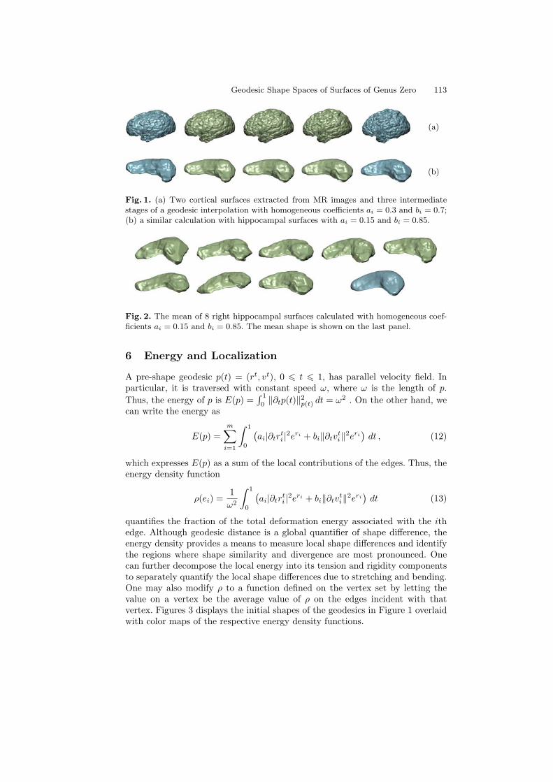
Geodesic Shape Spaces of Surfaces of Genus Zero 113
(a)
(b)
Fig. 1. (a) Two cortical surfaces extracted from MR images and three intermediatestages of a geodesic interpolation with homogeneous coefficients ai = 0.3 and bi = 0.7;(b) a similar calculation with hippocampal surfaces with ai = 0.15 and bi = 0.85.
Fig. 2. The mean of 8 right hippocampal surfaces calculated with homogeneous coef-ficients ai = 0.15 and bi = 0.85. The mean shape is shown on the last panel.
6 Energy and Localization
A pre-shape geodesic p(t) = (rt, vt), 0 6 t 6 1, has parallel velocity field. Inparticular, it is traversed with constant speed ω, where ω is the length of p.Thus, the energy of p is E(p) =
∫ 1
0‖∂tp(t)‖2
p(t) dt = ω2 . On the other hand, wecan write the energy as
E(p) =m∑
i=1
∫ 1
0
(ai|∂tr
ti |2eri + bi‖∂tv
ti‖2eri
)dt , (12)
which expresses E(p) as a sum of the local contributions of the edges. Thus, theenergy density function
ρ(ei) =1ω2
∫ 1
0
(ai|∂tr
ti |2eri + bi‖∂tv
ti‖2eri
)dt (13)
quantifies the fraction of the total deformation energy associated with the ithedge. Although geodesic distance is a global quantifier of shape difference, theenergy density provides a means to measure local shape differences and identifythe regions where shape similarity and divergence are most pronounced. Onecan further decompose the local energy into its tension and rigidity componentsto separately quantify the local shape differences due to stretching and bending.One may also modify ρ to a function defined on the vertex set by letting thevalue on a vertex be the average value of ρ on the edges incident with thatvertex. Figures 3 displays the initial shapes of the geodesics in Figure 1 overlaidwith color maps of the respective energy density functions.
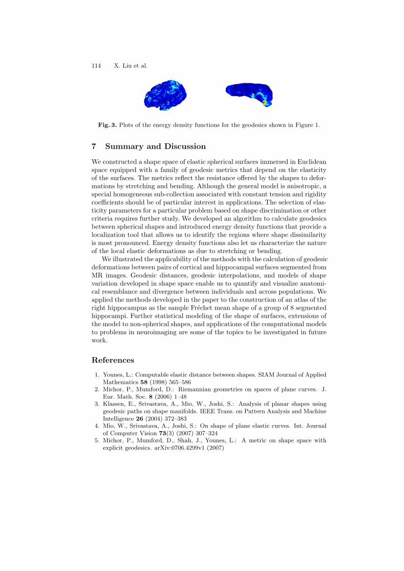
114 X. Liu et al.
Fig. 3. Plots of the energy density functions for the geodesics shown in Figure 1.
7 Summary and Discussion
We constructed a shape space of elastic spherical surfaces immersed in Euclideanspace equipped with a family of geodesic metrics that depend on the elasticityof the surfaces. The metrics reflect the resistance offered by the shapes to defor-mations by stretching and bending. Although the general model is anisotropic, aspecial homogeneous sub-collection associated with constant tension and rigiditycoefficients should be of particular interest in applications. The selection of elas-ticity parameters for a particular problem based on shape discrimination or othercriteria requires further study. We developed an algorithm to calculate geodesicsbetween spherical shapes and introduced energy density functions that provide alocalization tool that allows us to identify the regions where shape dissimilarityis most pronounced. Energy density functions also let us characterize the natureof the local elastic deformations as due to stretching or bending.
We illustrated the applicability of the methods with the calculation of geodesicdeformations between pairs of cortical and hippocampal surfaces segmented fromMR images. Geodesic distances, geodesic interpolations, and models of shapevariation developed in shape space enable us to quantify and visualize anatomi-cal resemblance and divergence between individuals and across populations. Weapplied the methods developed in the paper to the construction of an atlas of theright hippocampus as the sample Frechet mean shape of a group of 8 segmentedhippocampi. Further statistical modeling of the shape of surfaces, extensions ofthe model to non-spherical shapes, and applications of the computational modelsto problems in neuroimaging are some of the topics to be investigated in futurework.
References
1. Younes, L.: Computable elastic distance between shapes. SIAM Journal of AppliedMathematics 58 (1998) 565–586
2. Michor, P., Mumford, D.: Riemannian geometries on spaces of plane curves. J.Eur. Math. Soc. 8 (2006) 1–48
3. Klassen, E., Srivastava, A., Mio, W., Joshi, S.: Analysis of planar shapes usinggeodesic paths on shape manifolds. IEEE Trans. on Pattern Analysis and MachineIntelligence 26 (2004) 372–383
4. Mio, W., Srivastava, A., Joshi, S.: On shape of plane elastic curves. Int. Journalof Computer Vision 73(3) (2007) 307–324
5. Michor, P., Mumford, D., Shah, J., Younes, L.: A metric on shape space withexplicit geodesics. arXiv:0706.4299v1 (2007)

Geodesic Shape Spaces of Surfaces of Genus Zero 115
6. Praun, E., Hoppe, H.: Spherical parametrization and remeshing. In: ACM SIG-GRAPH 2003. (2003) 340–349
7. Shi, Y., Thompson, P., Dinov, I., Osher, S., Toga, A.: Direct cortical mapping viasolving partial differential equations on implicit surfaces. Medical Image Analysis11(3) (2007) 207–223
8. Shi, Y., Thompson, P., Zubicaray, G., Ross, S., Tu, Z., Dinov, I., Toga, A.: Directmapping of hippocampal surfaces with intrinsic shape context. NeuroImage 36(3)(2007) 792–807
9. Kendall, D.G.: Shape manifolds, Procrustean metrics and complex projectivespaces. Bulletin of London Mathematical Society 16 (1984) 81–121
10. Grenander, U., Miller, M.I.: Computational anatomy: An emerging discipline.Quarterly of Applied Mathematics LVI(4) (1998) 617–694
11. Fletcher, P., Lu, C., Pizer, S., Joshi, S.: Principal geodesic analysis for the study ofnonlinear statistics of shape. IEEE Transactions on Medical Imaging 23(8) (2004)995–1005
12. Palais, R.S.: Morse theory on Hilbert manifolds. Topology 2 (1963) 299–34013. do Carmo, M.P.: Riemannian Geometry. Birkhauser (1994)
A Closest-Shape Projection
Given (r, v) ∈ M near the pre-shape space P , we need an efficient estimation ofthe pre-shape closest to (r, v). Consider the kn + 1 residual functions ρ1(r, v) =1−G1(r, v) and ρ`,j(r, v) = −G`,j(r, v), whose vanishing is equivalent to (r, v) ∈P . We estimate the closest pre-shape using Newton’s method to find the zerosof H(r, v) = 1
2ρ21(r, v) + 1
2
∑`,j ρ2
`,j(r, v). If we relax the condition that each rowof v must satisfy ‖vi‖ = 1 and just treat each vi as an arbitrary vector in Rk,then the negative gradient of H is
−∇H(r, v) = ρ1(r, v)∇G1(r, v) +∑`,j
ρ`,j(r, v)∇G`,j(r, v) , (14)
where ∇Gr1(r, v) = [1/a1 . . . 1/am]T is the modular component of ∇G1(r, v) and
the directional component is zero. The modular part of ∇G`,j(r, v) and the jthcolumn of its directional component, which is its only nonzero column, are[
0 ε`1a`1
v`1,j 0 ε`2a`2
v`2,j 0 ε`3a`3
v`3,j 0]T
and[0 ε`1
b`10 ε`2
b`20 ε`3
b`30]T
. (15)
Here, the nonzero entries occur in rows `1, `2 and `3. Write the modular anddirectional parts of the gradient as −∇H(r, v) = (δr, δv). To make δv
i tan-gential to S2 at vi, replace it with δv
i = δvi − (δv
i · vi)vi. Letting ε(r, v) =H(r, v)/‖(δ1, δ2)‖2
(r,v), update (r, v) as follows:r = r + εδ1 ;vi = cos(ε‖δv
i ‖)vi + sin(ε‖δvi ‖)
‖δvi ‖
δvi , if δv
i 6= 0 ;(16)
and vi stays unchanged, otherwise. Iterate until H(r, v) becomes small.
116 X. Liu et al.
B Covariant Integration
For (z, y) = (z, y1, . . . , yk) ∈ R × Rk, we use the subscript 0 to identify thez-coordinate and the subscript j, 1 6 j 6 k, for the coordinate yj . Givenai, bi > 0, define a Riemannian metric on R × Rk whose metric tensor at (z, y)is g00(z, y) = aie
z, gjj(z, y) = biez, and 0, otherwise. Then, the Riemannian
structure on E, defined in Section 3, is isometric to the Cartesian product ofthese (k+1)-dimensional models over 1 6 i 6 m. Thus, to derive the differentialequation that governs covariant integration along a path in M , it suffices to de-rive the corresponding differential equation for covariant integration in R×Sk−1
with respect to the induced metric. The Christoffel symbols of the Levi-Civitaconnection on R × Rk are Γ 0
00 = Γ j0j = Γ j
j0 = 1/2, Γ 0jj = −bi/2ai, 1 6 j 6 k,
and zero otherwise. Therefore (cf. [13]), the covariant derivative of a vector field(F t, Xt) along a path (zt, yt) in R× Rk is given by
DtFt = ∂tF
t + 12 (∂tz
t)F t − 12
bi
ai[Xt · ∂ty
t]DtXt = ∂tX
t + 12 (Xt∂tz
t + F t∂tyt) .
(17)
If (zt, yt) is a path in R × Sk−1, then fields that are tangential to R × Sk−1 arethose that satisfy the additional orthogonality condition F t · yt = 0. Thus, if(f t, xt) and (F t, Xt) are both tangential to R×Sk−1, the fact that the covariantderivative of (F t, Xt) in the submanifold R× Sk−1 is (f t, xt) may be rephrasedas DtF
t = f t and DtXt = xt + τ tyt, where τ t is a scalar field to be determined.
Substituting in (17), we obtain∂tF
t = f t − 12∂tz
tF t + 12
bi
ai[Xt · ∂ty
t]∂tX
t = xt − 12 (Xt∂tz
t + F t∂tyt) + τ tyt .
(18)
Differentiating Xt · yt = 0, we get ∂tXt · yt = −Xt · ∂ty
t. From (18), it followsthat τ t = −Xt · ∂ty
t, where we used the facts that Xt · yt = 0 and ∂tyt · yt = 0.
Substituting this value of τ t in (18), we obtain (7).
Characterization of Anatomical Shape Based on
Random Walk Hitting Times
Grace Vesom1, Nathan D. Cahill1,2, Lena Gorelick3, and J. Alison Noble1
1 Institute of Biomedical Engineering, University of Oxford, Oxford OX3 HDQ, UK2 Research & Innovation, Carestream Health, Inc., Rochester, NY 14608, USA
3 Computer Vision Group, The Weizmann Institute of Science, Rehovot 76100, Israel
Abstract. This paper presents an implicit shape representation for de-scribing anatomical shapes with high inter-patient variability based onthe expected boundary hitting time of a random walk, which happens tobe the solution to the Poisson equation. The main contribution of thispaper is to test the validity of the Poisson-based mapping for learninganatomical shape variability, comparing its compactness and complete-ness with the commonly used Signed Distance Transform and using theliver and the caudate nucleus as examples. Based on these findings, wediscuss its use as a shape prior for image segmentation.
1 Introduction
An integral part of modern disease management is treatment planning, whichinvolves several aspects of medical image analysis, from segmenting objects ofinterest for volume measurement to intra-patient registration for monitoring sizechange or morphology. Because of the difficulty of these tasks, many segmenta-tion or registration frameworks require a shape representation for the object inquestion. Shape representations can be abstractly divided into two categories:explicit and implicit. Explicit shape representations are parameterized to createordered collections of components. Examples include Active Shape Models [1]and spherical harmonics [2]. Mostly, they define a (N −1)-dimensional boundaryin a N -dimensional image space, but can include additional information such asa medial representation [3] or, like Active Appearance Models [4], intensity andtexture.
An implicit representation of an N -dimensional shape is a function f(x) inan N -dimensional space that takes on the value zero if and only if x is a positionon the (N − 1)-dimensional shape boundary. The function is defined over theinside domain of the closed object, and sometimes, depending on the application,over the entire image domain.
Implicit shape descriptions are free of topological constraints and have localsupport. In recent literature, the Signed Distance Transform (SDT) has provedto be a popular implicit shape representation – attractive for ease of compu-tation, definition over the entire image space, and ability to fit into a level-setsegmentation framework. In addition to the SDT, Hong et al. [5] developed an
118 G. Vesom et al.
implicit shape representation based on an approximation to the solution of theheat equation over the shape. Their shape representation is attractive becauseit can be quickly computed by convolution with a Gaussian kernel. However, itdoes not adjust the Gaussian kernel to account for arbitrary shape boundaries.
To be able to summarize anatomical object variability, we seek a shape de-scriptor which can extract characteristic global object structure while preservingindividual variations. In our work, we consider another implicit shape represen-tation called the Poisson Transform (PT) and look at its application in learningand modeling anatomical variation. The PT was first used by Gorelick et al. [6]to analyze 2D shape properties on silhouettes in order to perform shape classifi-cation and retrieval. We extended that idea in [7] to include the shape exteriorand used this in the context of deformable image registration. In the next section,we revisit the mathematical representation of the SDT, then provide a summaryof and computational method for the PT. We use this new mapping to producean implicit shape representation, and then analyze it for completeness and com-pactness in comparison to the SDT. We use Principal Component Analysis onthe SDT for our training data to summarize shape variation in the same manneras [8–10]. We investigate the validity of the SDT representation for anatomicalobjects with highly variable shape against the PT representation. Besides thetechnical report by Lamecker et al. [11], no studies have assessed the compact-ness or completeness of liver shape description. We conclude by discussing itsapplication to image segmentation.
2 Implicit Shape Representations
Let us define S to be the interior of the shape and assume that S ⊂ Ω, whereΩ is the entire image space. Then ∂S = S − S is the boundary of S, where Srepresents the closure of the open set S.
2.1 Signed Distance Transform
The SDT, also known as the signed Euclidean distance transform, is representedhere by WSDT . It yields two pieces of information; the magnitude provides theEuclidean distance between a point and the closest point on ∂S, and the signindicates whether the current point is inside S (negative) or outside S (positive).Mathematically speaking, WSDT is a solution to the Eikonal equation:
|∇WSDT(x)| = 1 ∀x ∈ Ω,
WSDT(x) = 0 ∀x ∈ ∂S. (1)
Examples of the SDT for the liver and caudate nucleus can be seen in Figs.1(a) and 1(c).
Anatomical Shape through Random Walk Hitting Times 119
2.2 Random Walk Hitting Time
Gorelick et al. [6] presented an implicit shape representation based on the ex-pected time for a symmetric random walk to reach the shape boundary. Basedon the solution to Poisson’s equation, this representation has several advantagesas it is differentiable everywhere and has the interior regularity property.
In order to derive the Poisson Transform, consider a shape S defined ona 3-dimensional discrete lattice with isotropic spacing h. Now consider a par-ticle initially at position (x, y, z) ∈ S. If the particle undergoes a symmetricrandom walk, then we define U(x, y, z) to be the expected time (in number ofsteps) for the particle to reach any point on the boundary of S, given that theparticle started at (x, y, z). This expected time is also known as the ”hittingtime” because it represents the average time it will take the particle to ”hit” theboundary. Therefore, if (x, y, z) ∈ ∂S, then U(x, y, z) = 0. If (x, y, z) ∈ S, thenthe hitting time at (x, y, z) can be related to the hitting time at each of its sixneighbors by a conditioning argument:
U(x, y, z) = 1 +1
6
(
U(x + h, y, z) + U(x − h, y, z)
U(x, y + h, z) + U(x, y − h, z) (2)
U(x, y, z + h) + U(x, y, z − h))
.
Note that (2) is a discretized version of the Poisson equation
∆U(x, y, z) = −6
h2, (3)
with ∆U = Uxx + Uyy + Uzz denoting the Laplacian of U . For simplicity, wechose h = 1.
To use comparable notation with the SDT definition, let WPT replace U torepresent the symmetric random walk hitting time to the shape boundary inan open domain, and let x = (x, y, z) for the remainder of this paper. Like theSDT, we seek to use the sign of the metric values to define points inside andoutside the boundary shape, which results in changing the sign of (3), while themagnitude of those values still provides the symmetric random walk time to apoint on the boundary. Thus, for the shape interior, the Poisson Transform WPT
satisfies
∆WPT(x) = 6 ∀x ∈ S,
WPT(x) = 0 ∀x ∈ ∂S. (4)
On the exterior of the shape, if no further boundary conditions are prescribed,the random walk analogy fails and the Poisson equation has infinitely manysolutions. Therefore, in order to provide an extension of this shape representationto the entirety of Ω, we need to define some sort of external boundary condition.One option is to enforce Neumann boundary conditions on ∂Ω; however, thischoice gives undesirable behavior of the gradient of the Poisson Transform at the

120 G. Vesom et al.
image boundaries. Instead, we choose to define an open sphere T ⊃ Ω centeredon the centroid of Ω, and solve the following boundary value problem:
∆WPT(x) = −6 ∀x ∈ T − S,
〈∇WPT(x) ,n(x)〉 = 0 ∀x ∈ ∂T, (5)
WPT(x) = 0 ∀x ∈ ∂S,
where n(x) is the outward pointing normal vector to the surface ∂T at x. TheNeumann boundary condition on ∂T effectively reflects the symmetric randomwalk in the direction normal to the sphere. Once WPT has been found on T , itcan be cropped to Ω.
Computing a discrete approximation of WPT inside S can be done in lineartime with a multigrid algorithm [6]. This algorithm can be extended to approx-imate WPT inside T − S by appropriately discretizing the Neumann boundaryconditions, as established by Cahill et al. [7]. We have found that applying twow-cycles that employ naive boundary conditions at the coarse levels (placingthe boundary at the nearest coarse grid points, instead of modifying the nearbycoarse equations to account for the fine, pixel-level location of the boundary)provides a good approximation. For further details on the multigrid method, see[12].
Examples of the SDT for the liver and caudate nucleus can be seen in Figs.1(b) and 1(d).
(a) SDT (b) PT (c) SDT (d) PT
Fig. 1. Slices from example 3D liver and caudate nucleus images of both implicit func-tions, inside and outside the shape
3 Application to Segmentation
In medical image segmentation, image data information is typically balancedby integrating a priori knowledge into the algorithm through a shape prior,providing a global constraint in a segmentation framework.
Anatomical Shape through Random Walk Hitting Times 121
3.1 Shape Representation
Using a shape prior for image segmentation requires an application-specificchoice of shape representation. Selecting a shape representation or descriptoris a function of the information to be extracted from an image, the signal-to-noise of the image, the anatomical object in question, and the ultimate goalof the task. For the purpose of segmentation, the shape descriptor also subse-quently affects the dissimilarity measure for comparing shapes and method ofintegration for a model into a segmentation framework. Golland et al. [13] foundthat the choice of shape representation changed their classifier function resultsby about 15%, independent of shape analysis and alignment.
3.2 Shape Analysis Methods
With highly variable anatomical shapes, large numbers of samples, or trainingshapes, are required to correctly portray a shape population. Shape models areused to efficiently summarize the training shape space.
Much research looks for the best shape analysis method to summarize theshape space, while some methods never question the validity of its use, such aswith Principal Component Analysis (PCA). That method is utilized to reducethe dimensionality of the training shape space, while preserving the most vari-ation. PCA is often challenged because of its sensitivity to low sample size, aswell as the assumption of a Gaussian uni-modal distribution for the featuresmeasured in the resulting model. In the case of the SDT and PT, the shaperepresentation space is not closed under linear operations, but PCA is still oftenemployed. Shape analysis alternatives include independent component analysis[14], principal factor analysis [15], and support vector machines [13]. Addition-ally, methods to work around obstacles in PCA have shown some success. Theytransform training data into a feature space via Mercer kernels [16], or into avector space using Fourier approximation [17] or the logarithm of odds ratio [18],where linear operations of shape representation transformations are closed.
With the SDT, PCA has been consistently employed for shape analysis forthe purpose of learning shape variability in creating a statistical shape model.Notwithstanding, Hong et al. [5] used their integral kernel shape representationas a template with a deformation field for segmentation, removing the need forany shape analysis.
3.3 Implicit Anatomical Shape Priors
In image segmentation of highly variable shapes, it is essential to integrate apriori information as a global constraint with data-driven energy functions. Weconcentrate here on statistical shape models (SSMs), as opposed to deformableshape models or classifiers.
Leventon et al. [8] employed SSMs from implicit shape representations, usingthe SDT to represent shapes and PCA to summarize the shape space to createa shape prior in image segmentation. Thereafter, literature involving implicit

122 G. Vesom et al.
shape models concentrates on shape alignment prior to PCA and shape priorintegration into a region-based level-set segmentation framework. Rousson et al.[10] used the sum of squared distances as a dissimilarity measure between theprior and target, while minimizing the rotation and translation pose parametersduring the level set evolution. Tsai et al. [9] similarly proposed an alignmentmethod, but also included scale as a pose parameter and explored three energyfunctionals, optimizing the functionals via gradient descent. Yang et al. [19] tookanother step by introducing neighbor priors, developing a hierarchical multi-object segmentation. Accounting for neighboring structures in the shape prior,however, gave rise to concerns about closedness of linear combination of signeddistance functions. Neighboring structures were modeled by the difference oftheir representative SDTs, however any linear combination of these differencesmay not represent neighboring structures as mutually exclusive.
3.4 Analysis of Implicit Shape Representations SDT and PT
While any dimensionality reduction method can arguably be more suitable forshape analysis, we wish to show that a shape descriptor that suppresses redun-dancy in variability, yet elicits distinguishing global features, will result in moremeaningful factors. PCA is the most widely used form of shape analysis in med-ical imaging because of its ease of computation and interpretation. For thesereasons, we have thus chosen to use PCA for a comparative shape analysis studyon the SDT and PT.
The nature of the PT allows us to combine global and local shape extraction– we can see a common shape for each structure, while local variations arepreserved closer to the boundary (Figs. 3(b) and 2(b)). Consequently, we believePT is best suited to represent objects with high shape variability, for which theliver and caudate nucleus are well known and well studied.
(a) Signed distance function (b) Poisson function
Fig. 2. Inside level sets of the liver from SDT and PT

Anatomical Shape through Random Walk Hitting Times 123
(a) Signed distance function (b) Poisson function
Fig. 3. Inside level sets of the caudate nucleus from SDT and PT
Consider the case of representing the shape of the liver. Although liver shapehas consistent convexities, concavities, and ridges, it is still very highly variableacross the population. It is also adjacent to structures of similar density, makingit extremely difficult to segment in Computed Tomography (CT) images. Liverimage segmentation has been a well-established problem in medical imaginganalysis. A variety of published methods range from deformable models usingthe evolutionary algorithm [20] and data-driven methods [21] to graph-cuts [22],demonstrating the difficulty of the task.
The shape of the caudate nucleus is often investigated in order to identifybrain abnormalities. An irregular shape in longitudinal studies and intra-patientasymmetric shape can reveal developmental disorders, such as schizophrenia [23].
In 3D, we computed the SDT and PT for 33 liver images and 20 caudatenucleus images. Slices through the mapping for each transform and class areshown in Fig. 1, and 3D renderings of the inner level sets are shown in Figs. 3and 2.
3.5 The Data
Our data has been obtained from the MICCAI 3D Segmentation Challenge [24]and the Churchill Hospital, part of the Oxford Radcliffe Hospitals NHS Trustin Oxford, UK. We used the segmented training data sets from MICCAI, andwe manually segmented the additional liver data sets subject to the approvalof a clinician. All binary images were rescaled to physical Cartesian coordinatesand smoothed to remove aliasing effects. The liver surfaces were aligned as bi-nary images using the Principal Axis Transformation [25], while the caudatenucleus shapes were aligned using first-order moments, with a few slight manualrotations.
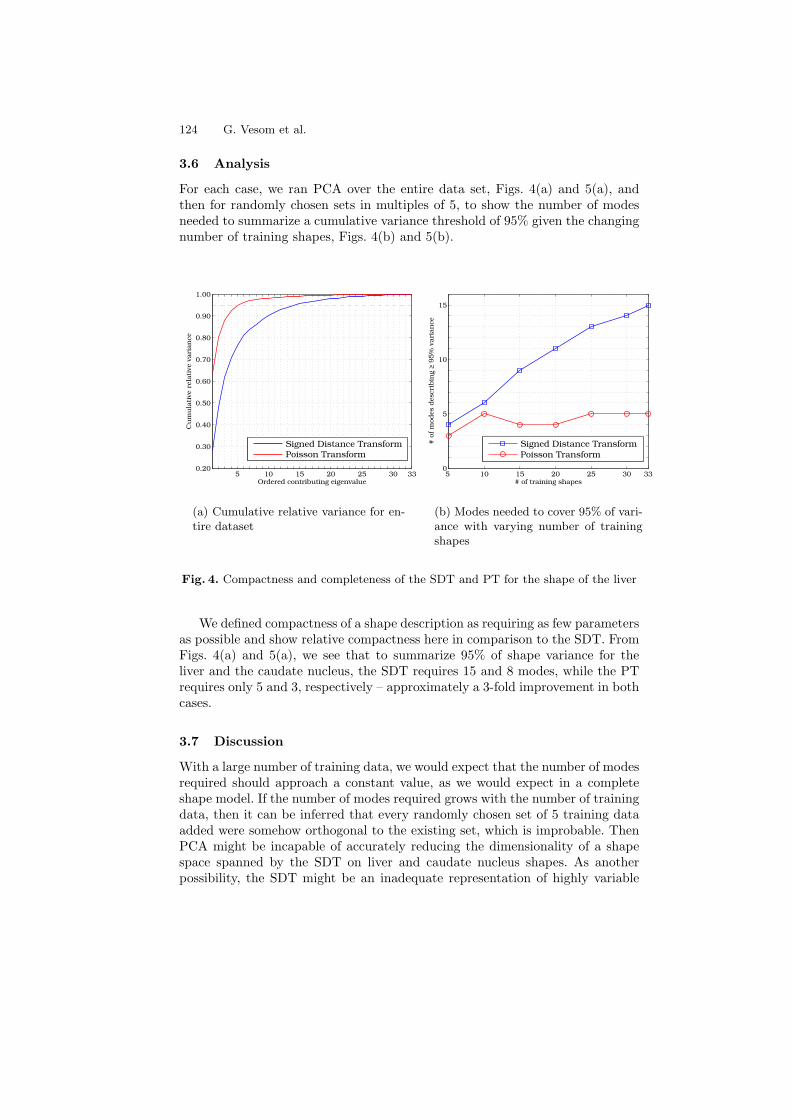
124 G. Vesom et al.
3.6 Analysis
For each case, we ran PCA over the entire data set, Figs. 4(a) and 5(a), andthen for randomly chosen sets in multiples of 5, to show the number of modesneeded to summarize a cumulative variance threshold of 95% given the changingnumber of training shapes, Figs. 4(b) and 5(b).
5 10 15 20 25 30 330.20
0.30
0.40
0.50
0.60
0.70
0.80
0.90
1.00
Ordered contributing eigenvalue
Cu
mu
lati
ve r
ela
tive v
ari
an
ce
Signed Distance TransformPoisson Transform
(a) Cumulative relative variance for en-tire dataset
5 10 15 20 25 30 330
5
10
15
# of training shapes
# o
f m
odes d
escri
bin
g ≥
95%
vari
an
ce
Signed Distance Transform
Poisson Transform
(b) Modes needed to cover 95% of vari-ance with varying number of trainingshapes
Fig. 4. Compactness and completeness of the SDT and PT for the shape of the liver
We defined compactness of a shape description as requiring as few parametersas possible and show relative compactness here in comparison to the SDT. FromFigs. 4(a) and 5(a), we see that to summarize 95% of shape variance for theliver and the caudate nucleus, the SDT requires 15 and 8 modes, while the PTrequires only 5 and 3, respectively – approximately a 3-fold improvement in bothcases.
3.7 Discussion
With a large number of training data, we would expect that the number of modesrequired should approach a constant value, as we would expect in a completeshape model. If the number of modes required grows with the number of trainingdata, then it can be inferred that every randomly chosen set of 5 training dataadded were somehow orthogonal to the existing set, which is improbable. ThenPCA might be incapable of accurately reducing the dimensionality of a shapespace spanned by the SDT on liver and caudate nucleus shapes. As anotherpossibility, the SDT might be an inadequate representation of highly variable
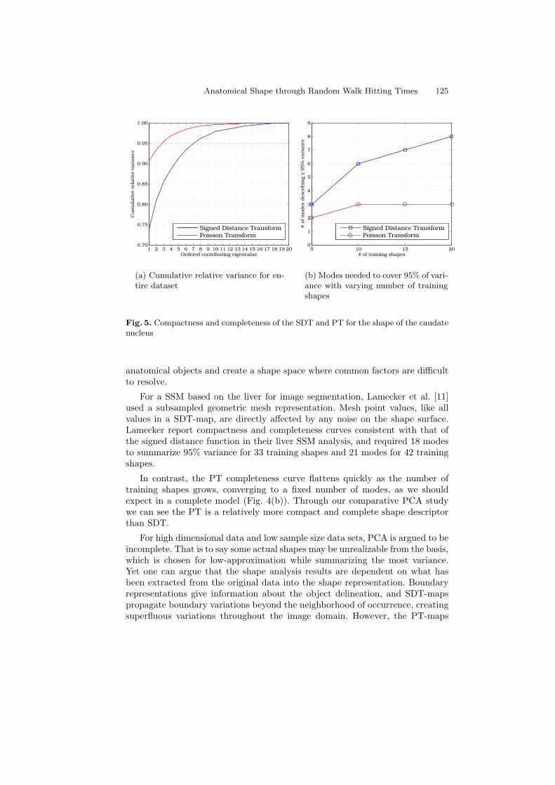
Anatomical Shape through Random Walk Hitting Times 125
1 2 3 4 5 6 7 8 9 10 11 12 13 14 15 16 17 18 19 200.70
0.75
0.80
0.85
0.90
0.95
1.00
Ordered contributing eigenvalue
Cu
mu
lati
ve r
ela
tive v
ari
an
ce
Signed Distance TransformPoisson Transform
(a) Cumulative relative variance for en-tire dataset
5 10 15 200
1
2
3
4
5
6
7
8
9
# of training shapes
# o
f m
odes d
escri
bin
g ≥
95%
vari
an
ce
Signed Distance TransformPoisson Transform
(b) Modes needed to cover 95% of vari-ance with varying number of trainingshapes
Fig. 5. Compactness and completeness of the SDT and PT for the shape of the caudatenucleus
anatomical objects and create a shape space where common factors are difficultto resolve.
For a SSM based on the liver for image segmentation, Lamecker et al. [11]used a subsampled geometric mesh representation. Mesh point values, like allvalues in a SDT-map, are directly affected by any noise on the shape surface.Lamecker report compactness and completeness curves consistent with that ofthe signed distance function in their liver SSM analysis, and required 18 modesto summarize 95% variance for 33 training shapes and 21 modes for 42 trainingshapes.
In contrast, the PT completeness curve flattens quickly as the number oftraining shapes grows, converging to a fixed number of modes, as we shouldexpect in a complete model (Fig. 4(b)). Through our comparative PCA studywe can see the PT is a relatively more compact and complete shape descriptorthan SDT.
For high dimensional data and low sample size data sets, PCA is argued to beincomplete. That is to say some actual shapes may be unrealizable from the basis,which is chosen for low-approximation while summarizing the most variance.Yet one can argue that the shape analysis results are dependent on what hasbeen extracted from the original data into the shape representation. Boundaryrepresentations give information about the object delineation, and SDT-mapspropagate boundary variations beyond the neighborhood of occurrence, creatingsuperfluous variations throughout the image domain. However, the PT-maps
126 G. Vesom et al.
reveal global shape information from a data set yet adapt to individual objectboundaries (see Figs. 1–2).
4 Conclusion and Future Work
In this paper, we introduced using a new implicit shape representation calledthe Poisson Transform, an extrapolation of Gorelick’s innovative approach toshape characterization. In our comparative dimensionality reduction study, weshowed that the PT gives approximately a 3-fold improvement over the SDT inthe number of principal components required to represent 95% of the liver andcaudate nucleus data set variance. The PT is capable of local support on theboundary for individual instances but substantially stable against those varia-tions to give rise to a characteristic object shape across a data set. This balancein description enables optimized learning for highly variable anatomical objects.We are currently working on methods of integrating a shape model based on thePT into an image segmentation framework and overcoming obstacles mentionedin [13, 18].
Acknowledgments
The authors would like to thank Professor J. M. Brady for his insightful discus-sions; Tobias Heimann, Martin Styner, and Bram van Ginneken for allowing usto use their data; and Dr. Joanne Brady from the Churchill Hospital in Oxfordfor selecting patients and overseeing manual segmentations.
References
1. Cootes, T., Taylor, C., Cooper, D., Graham, J., et al.: Active shape models-theirtraining and application. Computer Vision and Image Understanding 61(1) (1995)38–59
2. Brechbuhler, C., Gerig, G., Kubler, O.: Parametrization of closed surfaces for 3-D shape description. Computer Vision and Image Understanding 61(2) (1995)154–170
3. Styner, M., Gerig, G.: Medial models incorporating object variability for 3D shapeanalysis. Information Processing in Medical Imaging (2001) 502–516
4. Cootes, T., Edwards, G., Taylor, C.: Active appearance models. IEEE Transactionson Pattern Analysis and Machine Intelligence 23(6) (2001) 681–685
5. Hong, B.W., Prados, E., Soatto, S., Vese, L.: Shape Representation based onIntegral Kernels: Application to Image Matching and Segmentation. In: Proc.CVPR. (2006) I: 833–840
6. Gorelick, L., Galun, M., Sharon, E., Basri, R., Brandt, A.: Shape Representationand Classification Using the Poisson Equation. Transactions on Pattern Analysisand Machine Intelligence 28(12) (2006) 1991–2005
7. Cahill, N.D., Vesom, G., Gorelick, L., Brady, J., Noble, J.A., Brady, J.M.: Inves-tigating Implicit Shape Representations for Alignment of Livers from Serial CTExaminations. In: Proc. International Symposium on Biomedical Imaging. (May2008)
Anatomical Shape through Random Walk Hitting Times 127
8. Leventon, M.E., Grimson, W.E.L., Faugeras, O.: Statistical shape influence ingeodesic active contours. In: Computer Vision and Pattern Recognition, 2000.Proceedings. IEEE Conference on. Volume 1. (2000) 316–323
9. Tsai, A., Yezzi Jr, A., Wells, W., Tempany, C., Tucker, D., Fan, A., Grimson, W.,Willsky, A.: A shape-based approach to the segmentation of medical imagery usinglevel sets. Medical Imaging, IEEE Transactions on 22(2) (2003) 137–154
10. Rousson, M., Paragios, N., Deriche, R.: Implicit Active Shape Models for 3DSegmentation in MR Imaging. In: MICCAI 2004. Volume 3216., Springer Berlin /Heidelberg (September 2004) 209–216
11. Lamecker, H., Lange, T., Seebass, M.: Segmentation of the Liver using a 3DStatistical Shape Model. Technical report, Zuse Institute Berlin (April 2004)
12. Trottenberg, U., Oosterlee, C.W., Schuller: Multigrid. Academic Press (2001)13. Golland, P., Grimson, W., Shenton, M., Kikinis, R.: Detection and analysis of
statistical differences in anatomical shape. Medical Image Analysis 9(1) (February2005) 69–86
14. Hyvarinen, A., Oja, E.: Independent component analysis: algorithms and applica-tions. Neural Networks 13(4-5) (2000) 411–430
15. Ballester, M., Linguraru, M., Aguirre, M., Ayache, N.: On the adequacy of principalfactor analysis for the study of shape variability. Proc. SPIE 5747 (2005) 1392–1399
16. Cremers, D., Kohlberger, T., Schnorr, C.: Shape statistics in kernel space for vari-ational image segmentation. Pattern Recognition 36(9) (September 2003) 1929–1943
17. Srivastava, A., Joshi, S.H., Mio, W., Liu, X.: Statistical shape analysis: clustering,learning, and testing. Pattern Analysis and Machine Intelligence, IEEE Transac-tions on 27(4) (2005) 590–602
18. Pohl, K.M., Fisher, J., Shenton, M., McCarley, R., Grimson, W., Kikinis, R., Wells,W.: Using the logarithm of odds to define a vector space on probabilistic atlases.Medical Image Analysis 11(5) (October 2007) 465–477
19. Yang, J., Staib, L.H., Duncan, J.S.: Neighbor-constrained segmentation with levelset based 3-D deformable models. Medical Imaging, IEEE Transactions on 23(8)(2004) 940–948
20. Heimann, T., Munzing, S., Meinzer, H., Wolf, I.: A Shape-Guided DeformableModel with Evolutionary Algorithm Initialization for 3D Soft Tissue Segmen-tation. In: Information Processing in Medical Imaging. Volume 4584. SpringerBerlin/Heidelberg (2007) 1–12
21. Soler, L., Delingette, H., Malandain, G., Montagnat, J., Ayache, N., Koehl, C.,Dourthe, O., Malassagne, B., Smith, M., Mutter, D., et al.: Fully automaticanatomical, pathological, and functional segmentation from CT scans for hepaticsurgery. Computer Aided Surgery 6(3) (2001) 131–142
22. Boykov, Y., Funka-Lea, G.: Graph Cuts and Efficient N-D Image Segmentation.International Journal of Computer Vision 70(2) (November 2006) 109–131
23. Levitt, J., Westin, C., Nestor, P., Estepar, R., Dickey, C., Voglmaier, M., Seidman,L., Kikinis, R., Jolesz, F., McCarley, R., et al.: Shape of caudate nucleus and itscognitive correlates in neuroleptic-naive schizotypal personality disorder. BiologicalPsychiatry 55(2) (2004) 177–184
24. van Ginneken, B., Heimann, T., Styner, M.: 3D Segmentation in the Clinic: AGrand Challenge. In van Ginneken, B., Heimann, T., Styner, M., eds.: 3D Seg-mentation in the Clinic: A Grand Challenge. (2007) 7–15
25. Alpert, N.M.: The Principal Axes Transformation–A Method for Image Registra-tion. Journal of Nuclear Medicine 31(10) (October 1990) 1717–1722
Tiling Manifolds with Orthonormal Basis
Moo K. Chung12, Anqi Qiu4, Brendon, M. Nacewicz2,Seth Pollak3, Richard J. Davidson23
1Department of Biostatistics and Medical Informatics,2Waisman Laboratory for Brain Imaging and Behavior,
3 Department of Psychology and PsychiatryUniversity of Wisconsin, Madison, USA
4Division of Bioengineering, Faculty of EngineeringNational University of Singapore, Singapore
Abstract. One main obstacle in building a sophisticated parametricmodel along an arbitary anatomical manifold is the lack of an easilyavailable orthonormal basis. Although there are at least two numericaltechniques available for constructing an orhonormal basis such as theLaplacian eigenfunction approach and the Gram-Smidth orthogonaliza-tion, they are computationally not so trivial and costly. We present arelatively simpler method for constructing an orthonormal basis for anarbitrary anatomical manifold. On a unit sphere, a natural orthonormalbasis is the spherical harmonics which can be easily computed. Assumingthe manifold is topologically equivalent to the sphere, we can establish asmooth mapping ζ from the manifold to the sphere. Such mapping canbe obtained from various surface flattening techniques. If we project thespherical harmonics to the manifold, they are no longer orthonormal.However, we claim that there exists an orthonormal basis that is thefunction of spherical harmonics and the spherical mapping ζ.
The detailed step by step procedures for the construction is given alongwith the numerical validation using amygdala surfaces as an illustration.As an application, we propose the pullback representation that recon-structs surfaces using the orthonormal basis obtained from an averagetemplate. The pullback representation introduces less inter-subject vari-ability and thus requires far less number of coefficients than the tradi-tional spherical harmonic representation. The source code used in thestudy is freely available athttp://www.stat.wisc.edu/∼mchung/research/amygdala.
1 Introduction
We present a novel orthonormal basis construction method for an arbitraryanatomical surface that is topologically equivalent to a sphere. The methodavoids the well known Gram-Smidth orthogonalization procedure [7], which isinefficient for high resolution polygonal meshes. In order to perform the Gram-Smidth orthogonalization as described in [7], for a surface mesh with n vertices,
Tiling Manifolds with Orthonormal Basis 129
we need to perform the Choleski decomposition as well as the inversion of matrixof size n×n. For a cortical mesh generated with FreeSurfer [6], n can easily reachup to 200000.
On the other hand, Qiu et al. [15] constructed an orthonormal basis as theeigenfunctions of the Laplace-Beltrami operator in a bounded regions of interest(ROI) on a cortical surface (Figure 3). The finite element method (FEM) is usedto numerically construct the orthonormal basis by solving a system of large linearequations. The weakness of the FEM approach is the computational burden ofinverting a matrix of size n×n. One advantage of the eigenfunction approach isthat since the eigenfunctions and eigenvalues are directly related to the Laplace-Beltrami operator, it is trivial and geometrically intuitive to construct the heatkernel analytically and perform a various heat kernel smoothing based modeling[4].
We propose a completely different method that avoids the computationalbottleneck by using a conceptually different machinery. We assume an arbitraryanatomical surface to be topologically equivalent to a sphere. Then using asmooth mapping ζ obtained from a surface flattening technique, we project thespherical harmonics to the anatomical surface. Obviously the projected spheri-cal harmonics will no longer be orthonormal. However, if we correct the metricdistortion introduced from the surface flattening, we may able to make the pro-jected spherical harmonics orthonormal somehow. This is the basic idea behindour new proposed method. For the surface flattening, we present a new methodthat treats the mapping ζ as the geodesic path of the heat equilibrium state.
As an application of the proposed technique, we present the novel pullback
representation for parameterizing anatomical boundaries that outperforms thetraditional spherical harmonic (SPHARM) representation [2] [3] [8] [16] [17]. Weclaim that our proposed representation has far less intersubject variability in theestimated parameters than SPHARM and converges faster to the true boundarywith less number of basis.
2 Methods
It is assumed that the anatomical boundary M is a smooth 2-dimensional Rie-mannian manifold parameterized by two parameters. The one-to-one mapping ζfrom point p = (p1, p2, p3)
′ ∈ M to u = (u1, u2, u3)′ ∈ S2, a unit sphere, can be
obtained from various surface flattening techniques such as conformal mapping[1] [8] [9], quasi-isometric mapping [18], area preserving mapping [2] [16] [17]and the deformable surface algorithm [13]. Since the conformal mapping tend tointroduce huge area distortion, most spherical harmonic literature tend to usearea preserving mapping [2] [16] [17].
In this paper, we present a new flattening technique via the geodesic trajec-tory of the equilibrium sate of heat diffusion. The proposed flattening techniqueis numerically simpler than any other available methods and does not requireoptimizing a cost function. The methodology is illustrated using the 47 amyg-
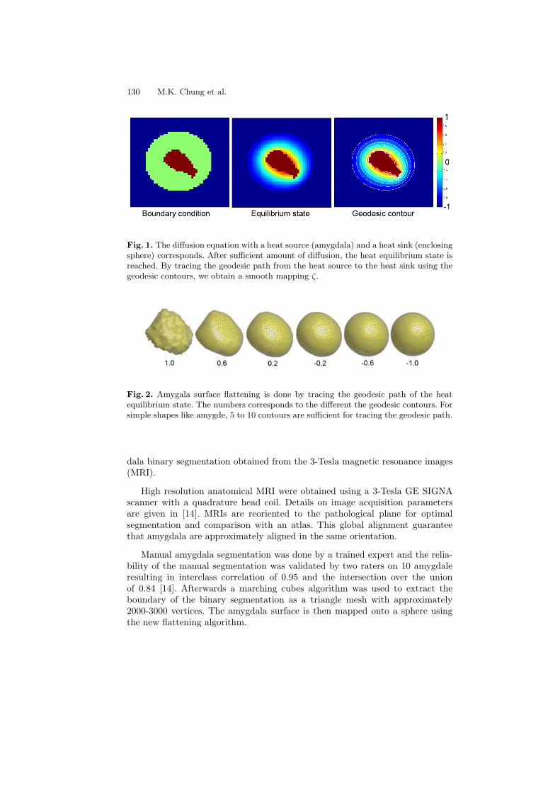
130 M.K. Chung et al.
Fig. 1. The diffusion equation with a heat source (amygdala) and a heat sink (enclosingsphere) corresponds. After sufficient amount of diffusion, the heat equilibrium state isreached. By tracing the geodesic path from the heat source to the heat sink using thegeodesic contours, we obtain a smooth mapping ζ.
Fig. 2. Amygala surface flattening is done by tracing the geodesic path of the heatequilibrium state. The numbers corresponds to the different the geodesic contours. Forsimple shapes like amygde, 5 to 10 contours are sufficient for tracing the geodesic path.
dala binary segmentation obtained from the 3-Tesla magnetic resonance images(MRI).
High resolution anatomical MRI were obtained using a 3-Tesla GE SIGNAscanner with a quadrature head coil. Details on image acquisition parametersare given in [14]. MRIs are reoriented to the pathological plane for optimalsegmentation and comparison with an atlas. This global alignment guaranteethat amygdala are approximately aligned in the same orientation.
Manual amygdala segmentation was done by a trained expert and the relia-bility of the manual segmentation was validated by two raters on 10 amygdaleresulting in interclass correlation of 0.95 and the intersection over the unionof 0.84 [14]. Afterwards a marching cubes algorithm was used to extract theboundary of the binary segmentation as a triangle mesh with approximately2000-3000 vertices. The amygdala surface is then mapped onto a sphere usingthe new flattening algorithm.

Tiling Manifolds with Orthonormal Basis 131
2.1 Diffusion-Based Surface Flattening
Given an amygdala binary segmentation Ma, we put a larger sphere Ms thatencloses the amygala (Figure 1 left). The amygdala and sphere serve as Dirichletboundary conditions for solving the Laplace equation. The amygdala is assignedthe value 1 while the enclosing sphere is assigned the value -1, i.e.
f(Ma, σ) = 1, f(Ms, σ) = −1 (1)
for all σ. The amygdala and the sphere serve as a heat source and a heat sinkrespectively. Then we solve an isotropic diffusion
∂f
∂σ= ∆f (2)
within the empty space bounded by the amygdala and the sphere. ∆ is the 3DLaplacian. After enough diffusion, the system reaches the heat equilibrium statewhere the additional diffusion does not make any difference in the heat distri-bution (Figure 1 middle). Once we obtained the equilibrium state, we trace thegeodesic path from the heat source to the heat sink for every mesh vertices. Thetrajectory of the geodesic path provides a smooth mapping from the amygdalasurface to the sphere. The geodesic path can be easily traced by constructinggeodesic contours that correspond to the level set of the equilibrium state (Figure1 right). Then the geodesic path is constructed by finding the shortest distancefrom one contour to the next and iteratively connecting the path together. Fig-ure 2 shows the process of flattening using five contours corresponding to thetemperature 0.6, 0.2, -0.2, -0.6, -1.0.
Although we did not apply our flattening technique to other anatomical ob-jects, the proposed method can be applied to more complex object than theamygdala. At the equilibrium state, we no longer has change in heat change overtime, i.e. ∂f
∂σ= 0, so we have the Laplace equation
∆f = 0
with the same boundary condition. The Laplace equation has been previouslyused to trace the distance between outer and inner cortical surfaces and to com-pute cortical thickness [10] [12] [19]. Since the solution to the Laplace equationwith the boundary condition (1) is unique even for highly convoluted and foldedstructures, the geodesic path will be uniquely defined.
2.2 Orhonormal basis in two sphere S2
Suppose a unit sphere S2 is represented as a high resolution triangle mesh con-sisting of the vertex set V(S2). We have used an almost uniformly sampled meshwith 2562 vertices and 5120 faces. Let us parameterize coordinates u ∈ S2 withparameters θ, ϕ:
(u1, u2, u3) = (sin θ cos ϕ, sin θ sin ϕ, cos θ),

132 M.K. Chung et al.
where (θ, ϕ) ∈ N = [0, π]⊗ [0, 2π). The polar angle θ is the angle from the northpole and ϕ is the azimuthal angle. The orthonormal basis on the unit sphere isgiven by the eigenfunctions of
∆f + λf = 0,
where ∆ is the spherical Laplacian. The eigenfunction Ylm corresponding to theeigenvalue l(l + 1) is called the spherical harmonic of degree l and order m [5].With respect to the inner product
〈f, g〉S2 =
∫
S2
f(u)g(u) dµ(u), (3)
with measure dµ(u) = sin θdθdϕ, Ylm form the orthonormal basis in L2(S2), thespace of square integrable functions on S2, i.e.
〈Ylm, Yl′m′〉S2 = δll′δmm′ . (4)
The inner product can be numerically computed as the Riemann sum overmesh vertices as
〈Ylm, Yl′m′〉S2 ≈∑
uj∈V(S2)
Ylm(uj)Yl′m′(uj)DS2(uj), (5)
where DS2(uj) is the discrete approximation of dµ(u). Let T 1uj
, T 2uj
, · · · , T jmuj
bethe area of triangles containing the vertex uj . Then we estimate DS2(uj) as
DS2(uj) =1
3
jm∑
k=1
T kuj
. (6)
The discrete approximation (6) defines the area of triangles at a mesh vertex.The factor 1/3 is chosen in such a way that
∑
uj∈V(S2)
DS2(uj) = 12.5514 = 4 · 3.1378,
analogous to the relationship∫
S2
dµ(p) = 4π.
The discrepancy between the integral and its discrete counter part is due to themesh resolution and it should become smaller as the mesh resolution increases.
Based on the proposed discretization scheme, we have computed the innerproduct (5) for all degrees 0 ≤ l, l′ ≤ 20. Figure 3 (left) shows the inner productsfor every possible pairs. Since for up to the k-th degree, there are total (k +1)2 basis functions, we have total 4412 possible inner product pairs, which isdisplayed as a matrix. For the diagonal terms, we obtained 0.9988±0.0017 whilefor the off-diagonal terms, we have obtained 0.0000±0.0005 indicating our basisand the discretization scheme is orthonormal with two decimal accuracy.
Tiling Manifolds with Orthonormal Basis 133
2.3 Orthonormal basis on manifold M
For f, g ∈ L2(M), the orthonormality is defined with respect to the inner product
〈f, g〉M =
∫
M
f(p)g(p) dµ(p).
Using the spherical harmonics in S2, it is possible to construct an orthonormalbasis in M numerically without the computational burden of solving the largematrix inversion associated with the eigenfunction method or the Gram-Smidthorthogonalization. Since the spherical harmonics are orthonormal in S2 and, themanifolds S2 and M can be deformed to each other by the mapping ζ, onewould guess that the orthonormal basis in M can be obtained somehow usingthe spherical harmonics. Surprisingly this guess is not wrong as we will show inthis section.
For f ∈ L2(S2), let us define the pullback operation ∗ as
ζ∗f = f ζ.
While f is defined on S2, the pullbacked function ζ∗f is defined on M. Theschematic of the pull back operation is given in Figure 6 (a). Then even thoughwe do not have orthonormality on the pullbacked spherical harmonics, i.e.,
〈ζ∗Ylm, ζ∗Yl′m′〉M 6= δll′δmm′ ,
we can make them orthonormal by using the Jacobian determinant of the map-ping ζ somehow.
Consider the Jacobian Jζ of the mapping ζ : p ∈ M → u ∈ S2 defined as
Jζ =∂u(θ, ϕ)
∂p(θ, ϕ).
For functions f, g ∈ L2(S2), we have the following change of variable relationship:
〈f, g〉S2 =
∫
M
ζ∗f(p)ζ∗g(p)|det Jζ | dµ(p). (7)
Similarly we have the inverse relationship given as
〈ζ∗f, ζ∗g〉M =
∫
S2
f(u)g(u)|det Jζ−1 | dµ(u). (8)
By letting f = Ylm and g = Yl′m′ in (7), we obtain
δll′δmm′ =
∫
M
ζ∗Ylmζ∗Yl′m′ |det Jζ | dµ(p) (9)
Equation (9) demonstrates that functions
Zlm = |det Jζ |1/2ζ∗Ylm (10)
are orthonormal in M. We will refer l as degree and m as order of the basisfunction. Using the Riesz-Fischer theorem [11], it is not hard to show that Zlm
form a complete basis in L2(M).
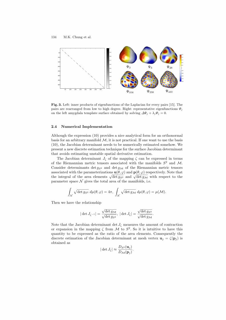
134 M.K. Chung et al.
50 100 150 200 250 300 350 400
50
100
150
200
250
300
350
400
0
0.1
0.2
0.3
0.4
0.5
0.6
0.7
0.8
0.9
1
Fig. 3. Left: inner products of eigenfunctions of the Laplacian for every pairs [15]. Thepairs are rearranged from low to high degree. Right: representative eigenfunctions Ψj
on the left amygdala template surface obtained by solving ∆Ψj + λjΨj = 0.
2.4 Numerical Implementation
Although the expression (10) provides a nice analytical form for an orthonormalbasis for an arbitrary manifold M, it is not practical. If one want to use the basis(10), the Jacobian determinant needs to be numerically estimated somehow. Wepresent a new discrete estimation technique for the surface Jacobian determinantthat avoids estimating unstable spatial derivative estimation.
The Jacobian determinant Jζ of the mapping ζ can be expressed in termsof the Riemannian metric tensors associated with the manifolds S2 and M.Consider determinants det gS2 and det gM of the Riemannian metric tensorsassociated with the parameterizations u(θ, ϕ) and p(θ, ϕ) respectively. Note thatthe integral of the area elements
√det gS2 and
√det gM with respect to the
parameter space N gives the total area of the manifolds, i.e.
∫
N
√
det gS2 dµ(θ, ϕ) = 4π,
∫
N
√
det gM dµ(θ, ϕ) = µ(M).
Then we have the relationship
|det Jζ−1 | =
√det gM√det gS2
, |det Jζ | =
√det gS2
√det gM
.
Note that the Jacobian determinant detJζ measures the amount of contractionor expansion in the mapping ζ from M to S2. So it is intuitive to have thisquantity to be expressed as the ratio of the area elements. Consequently thediscrete estimation of the Jacobian determinant at mesh vertex uj = ζ(pj) isobtained as
|det Jζ | ≈DS2(uj)
DM(pj).
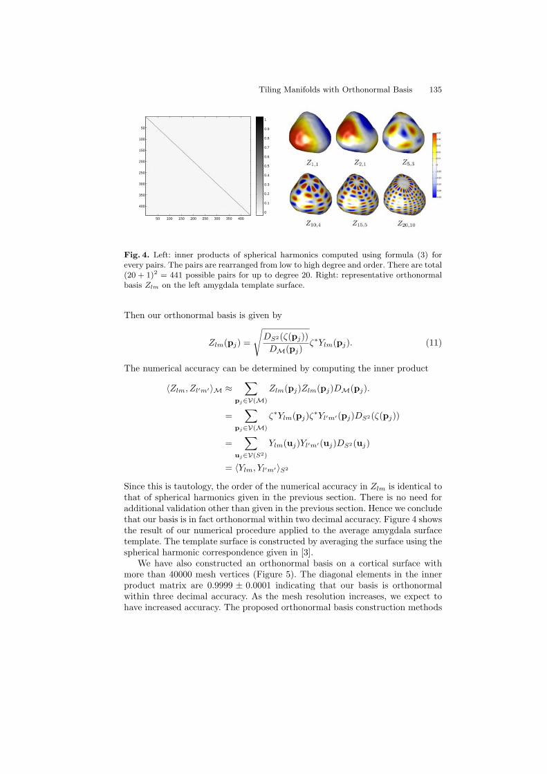
Tiling Manifolds with Orthonormal Basis 135
50 100 150 200 250 300 350 400
50
100
150
200
250
300
350
400
0
0.1
0.2
0.3
0.4
0.5
0.6
0.7
0.8
0.9
1
Fig. 4. Left: inner products of spherical harmonics computed using formula (3) forevery pairs. The pairs are rearranged from low to high degree and order. There are total(20 + 1)2 = 441 possible pairs for up to degree 20. Right: representative orthonormalbasis Zlm on the left amygdala template surface.
Then our orthonormal basis is given by
Zlm(pj) =
√
DS2(ζ(pj))
DM(pj)ζ∗Ylm(pj). (11)
The numerical accuracy can be determined by computing the inner product
〈Zlm, Zl′m′〉M ≈∑
pj∈V(M)
Zlm(pj)Zlm(pj)DM(pj).
=∑
pj∈V(M)
ζ∗Ylm(pj)ζ∗Yl′m′(pj)DS2(ζ(pj))
=∑
uj∈V(S2)
Ylm(uj)Yl′m′(uj)DS2(uj)
= 〈Ylm, Yl′m′〉S2
Since this is tautology, the order of the numerical accuracy in Zlm is identical tothat of spherical harmonics given in the previous section. There is no need foradditional validation other than given in the previous section. Hence we concludethat our basis is in fact orthonormal within two decimal accuracy. Figure 4 showsthe result of our numerical procedure applied to the average amygdala surfacetemplate. The template surface is constructed by averaging the surface using thespherical harmonic correspondence given in [3].
We have also constructed an orthonormal basis on a cortical surface withmore than 40000 mesh vertices (Figure 5). The diagonal elements in the innerproduct matrix are 0.9999 ± 0.0001 indicating that our basis is orthonormalwithin three decimal accuracy. As the mesh resolution increases, we expect tohave increased accuracy. The proposed orthonormal basis construction methods

136 M.K. Chung et al.
Fig. 5. Orthonormal basis Zlm on a cortical surface. The basis is projected on a sphereto show how the nonuniformity of the Jacobian determinant is effecting the sphericalharmonics Ylm. The color scale is thresholded at ±0.003 for better visualization.
avoids inverting matrix of size larger than 40000 × 40000 associated with theeigenfunction approach and the Gram-Smidth orthogonalization process.
Although the pattern of tiling in the eigenfunction approach (Figure 3) andthe pullback based method (Figure 4) looks different, it can be shown that theyare actually linearly dependent.
3 Application: Pullback Representation
As an application of the proposed orthonormal basis construction, we presenta new variance reducing Fourier Series representation that outperforms the tra-ditional spherical harmonic representation [2] [3] [8] [16] [17]. We will call thismethod as the pullback representation.
The spherical harmonic (SPHARM) representation models the surface coor-dinates with respect to a unit sphere as
p(θ, ϕ) =
k∑
l=0
l∑
m=−l
p0lmYlm(θ, ϕ) (12)
where p0lm = 〈p, Ylm〉S2 are spherical harmonic coefficients, which can be viewed
as random variables. The coefficients are estimated using the iterative residual
fitting algorithm [3] that breaks a larger least squares problem into smaller onesin an iterative fashion. The MATLAB code for performing the iterative residualfitting algorithm for arbitrary surface mesh is given in http://www.stat.wisc.edu
/∼mchung/softwares/weighted-SPHARM/weighted-SPHARM.hmtl. Note that all MRIswere reoriented to the pathological plane guaranteeing an approximate globalalignment before the surface flattening to increase the robustness of the coeffi-cient estimation.
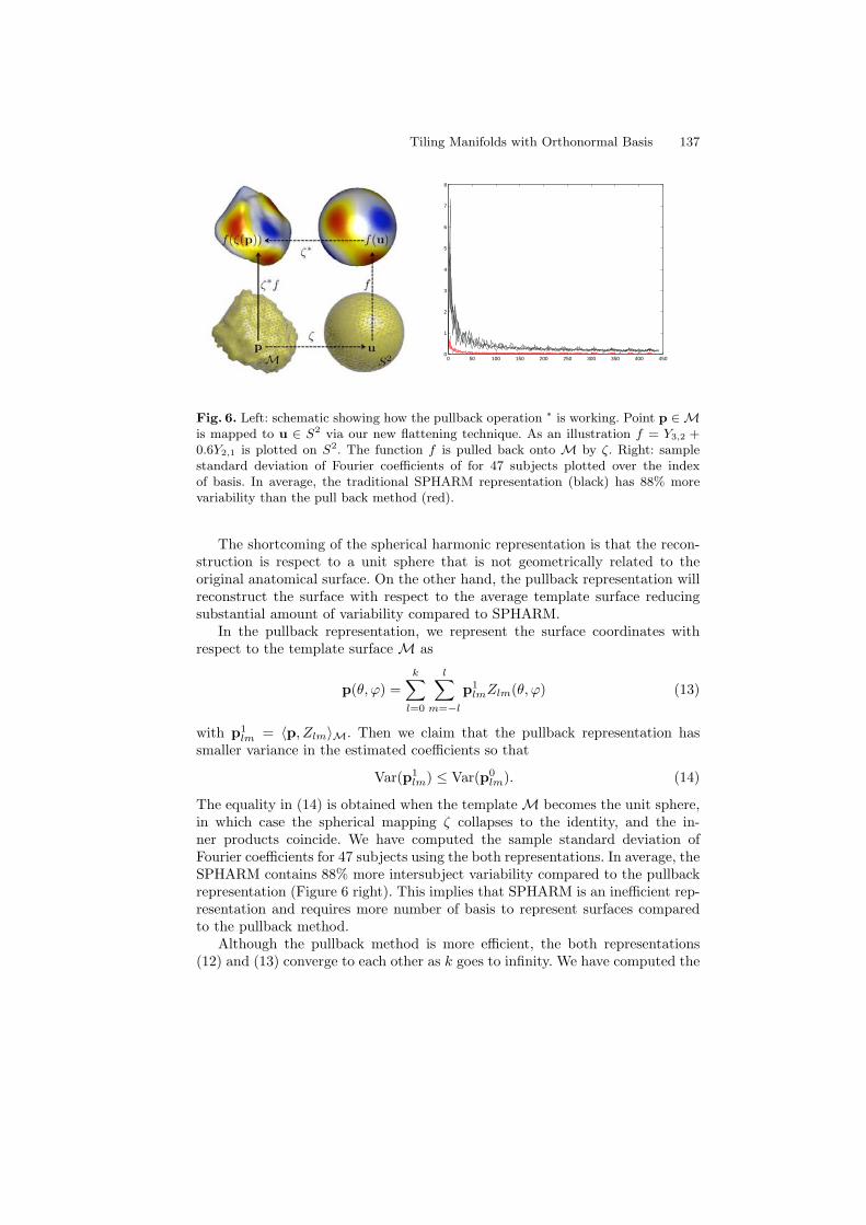
Tiling Manifolds with Orthonormal Basis 137
0 50 100 150 200 250 300 350 400 4500
1
2
3
4
5
6
7
8
Fig. 6. Left: schematic showing how the pullback operation ∗ is working. Point p ∈ Mis mapped to u ∈ S2 via our new flattening technique. As an illustration f = Y3,2 +0.6Y2,1 is plotted on S2. The function f is pulled back onto M by ζ. Right: samplestandard deviation of Fourier coefficients of for 47 subjects plotted over the indexof basis. In average, the traditional SPHARM representation (black) has 88% morevariability than the pull back method (red).
The shortcoming of the spherical harmonic representation is that the recon-struction is respect to a unit sphere that is not geometrically related to theoriginal anatomical surface. On the other hand, the pullback representation willreconstruct the surface with respect to the average template surface reducingsubstantial amount of variability compared to SPHARM.
In the pullback representation, we represent the surface coordinates withrespect to the template surface M as
p(θ, ϕ) =
k∑
l=0
l∑
m=−l
p1lmZlm(θ, ϕ) (13)
with p1lm = 〈p, Zlm〉M. Then we claim that the pullback representation has
smaller variance in the estimated coefficients so that
Var(p1lm) ≤ Var(p0
lm). (14)
The equality in (14) is obtained when the template M becomes the unit sphere,in which case the spherical mapping ζ collapses to the identity, and the in-ner products coincide. We have computed the sample standard deviation ofFourier coefficients for 47 subjects using the both representations. In average, theSPHARM contains 88% more intersubject variability compared to the pullbackrepresentation (Figure 6 right). This implies that SPHARM is an inefficient rep-resentation and requires more number of basis to represent surfaces comparedto the pullback method.
Although the pullback method is more efficient, the both representations(12) and (13) converge to each other as k goes to infinity. We have computed the

138 M.K. Chung et al.
Fig. 7. Comparison of SPHARM and the pullback representations for degree 5 to 25.Red colored numbers are the average Euclidean distance between two representationsin mm.
squared Euclidean distance between two representations numerically (Figure 7).In average, the difference is 0.0569 mm for 20 degree representation negligible for1mm resolution MR. Figure 7 also visually demonstrate that the pullback rep-resentation converges to the true manifold faster than SPHARM again showingthe inefficiency of the SPHARM representation.
4 Conclusion
We have introduced a computationally efficient way to construct an approxi-mate orthonormal basis on an arbitrary manifold by pulling back the sphericalharmonics to the manifold and accounting for the metric distortion using theJacobian determinant. The proposed technique is very general so that it can beapplicable to other types of anatomical manifolds. The constructed basis on anamygdala is used to show the new pullback representation that reconstruct themanifold as linear combination of the basis functions.
References
1. S. Angenent, S. Hacker, A. Tannenbaum, and R. Kikinis. On the laplace-beltramioperator and brain surface flattening. IEEE Transactions on Medical Imaging,18:700–711, 1999.
2. C. Brechbuhler, G. Gerig, and O. Kubler. Parametrization of closed surfaces for 3dshape description. Computer Vision and Image Understanding, 61:154–170, 1995.
3. M.K. Chung, L. Shen Dalton, K.M., A.C. Evans, and R.J. Davidson. Weightedfourier representation and its application to quantifying the amount of gray matter.IEEE Transactions on Medical Imaging, 26:566–581, 2007.
Tiling Manifolds with Orthonormal Basis 139
4. M.K. Chung, S. Robbins, Davidson R.J. Alexander A.L. Dalton, K.M., and A.C.Evans. Cortical thickness analysis in autism with heat kernel smoothing. Neu-
roImage, 25:1256–1265, 2005.5. R. Courant and D. Hilbert. Methods of Mathematical Physics: Volume II. Inter-
science, New York, english edition, 1953.6. B. Fischl and A.M. Dale. Measuring the thickness of the human cerebral cortex
from magnetic resonance images. PNAS, 97:11050–11055, 2000.7. K.M. Gorski. On determining the spectrum of primordial inhomogeneity from the
cobe dmr sky maps: I. method. Astrophysical Journal, 430, 430:L85, 1994.8. X. Gu, Y.L. Wang, T.F. Chan, T.M. Thompson, and S.T. Yau. Genus zero surface
conformal mapping and its application to brain surface mapping. IEEE Transac-
tions on Medical Imaging, 23:1–10, 2004.9. M. K. Hurdal and K. Stephenson. Cortical cartography using the discrete confor-
mal approach of circle packings. NeuroImage, 23:S119S128, 2004.10. S.E. Jones, B.R. Buchbinder, and I. Aharon. Three-dimensional mapping of cortical
thickness using laplace’s equation. Human Brain Mapping, 11:12–32, 2000.11. A.N. Kolmogorov and S.V. Fomin. Introductory real analysis. Dover Publications,
Inc, New York, 1970.12. J. P. Lerch and A.C. Evans. Cortical thickness analysis examined through power
analysis and a population simulation. NeuroImage, 24:163–173, 2005.13. J.D. MacDonald, N. Kabani, D. Avis, and A.C. Evans. Automated 3-D extraction
of inner and outer surfaces of cerebral cortex from mri. NeuroImage, 12:340–356,2000.
14. B.M. Nacewicz, K.M. Dalton, T. Johnstone, M.T. Long, E.M. McAuliff, T.R.Oakes, A.L Alexander, and R.J. Davidson. Amygdala volume and nonverbal socialimpairment in adolescent and adult males with autism. Arch. Gen. Psychiatry,63:1417–1428, 2006.
15. A. Qiu, D. Bitouk, and M.I. Miller. Smooth functional and structural maps on theneocortex via orthonormal bases of the laplace-beltrami operator. IEEE Transac-
tions on Medical Imaging, 25:1296–1396, 2006.16. L. Shen, J. Ford, F. Makedon, and A. Saykin. surface-based approach for clas-
sification of 3d neuroanatomical structures. Intelligent Data Analysis, 8:519–542,2004.
17. M. Styner, I. Oguz, S. Xu, C. Brechbuhler, D. Pantazis, J. Levitt, M. Shenton, andG. Gerig. Framework for the statistical shape analysis of brain structures usingspharm-pdm. In Insight Journal, Special Edition on the Open Science Workshop
at MICCAI, 2006.18. B. Timsari and R. Leahy. An optimization method for creating semi-isometric flat
maps of the cerebral cortex. In The Proceedings of SPIE, Medical Imaging, 2000.19. A. Yezzi and J.L. Prince. An eulerian pde approach for computing tissue thickness.
IEEE Transactions on Medical Imaging, 22:1332–1339, 2003.
Diffusion Tensor Imaging and Deconvolution on
Spaces of Positive Definite Symmetric Matrices
Peter T. Kim ⋆ and Donald St. P. Richards ⋆⋆
University of Guelph and Penn State University
Abstract. Diffusion tensor imaging can be studied as a deconvolutiondensity estimation problem on the space of positive definite symmetricmatrices. We develop a nonparametric estimator for the common densityfunction of a random sample of positive definite matrices. Our estimatoris based on the Helgason-Fourier transform and its inversion, the naturaltools for analysis of compositions of random positive definite matrices.Under smoothness conditions on the density of the intrinsic error in therandom sample, we derive bounds on the rates of convergence of ournonparametric estimator to the true density.
Key words: Deconvolution; diffusion tensor imaging; Harish-Chandrac-function; Helgason-Fourier transform; inverse problems; Laplace-Beltramioperator; magnetic resonance imaging; Sobolev spaces; Wishart distribu-tion.
1 Introduction
The appearance in medical imaging of sequences of random positive definite ma-trices has become commonplace due to developments in diffusion tensor imaging
(DTI), a method of imaging based upon the observation that water molecules inbiological tissue are always in motion. For the purposes of mathematical mod-eling, it is generally assumed that the diffusion of water molecules at any givenlocation in biological tissue follows a Brownian motion. A diffusion tensor imagethen is represented by the 3 × 3 positive-definite covariance matrix of the localdiffusion process at the given location (Fletcher and Joshi [3, 4]. DTI seeks todetect the diffusion of water protons between and within distinct tissue cells, andto derive estimates of the dominant orientation and direction of the Brownianmotion (Le Bihan [9], Hasan, et al. [5]).
In DTI brain imaging, the diffusion of water molecules within and betweenvoxels, the three-dimensional volume elements that constitute an image, reveal
⋆ Department of Mathematics and Statistics, University of Guelph, Guelph, OntarioN1G 2W1, Canada. Research supported in part by the Natural Sciences and Engi-neering Research Council of Canada, grant DG-46204. Email: [email protected].
⋆⋆ Department of Statistics, The Pennsylvania State University, University Park, PA16802. Research supported in part by the U.S. National Science Foundation, grantsDMS-0112069 and DMS-0705210. Email: [email protected].
DTI and Deconvolution 141
both the orientation of fibers comprising white-matter tracts in the brain andthe coherence of fibers, the extent to which fibers are aligned together. DTI maybe the only non-invasive, in vivo procedure which enables the study of deep brainwhite-matter fibers. Consequently, DTI has been found to be highly promisingfor comparing the human brain in normal states with abnormal states causedby strokes, epileptic seizures, tumors, white-matter abnormalities, multiple scle-rosis lesions, HIV-infection, traumatic brain injuries, aging, Alzheimer’s disease,alcoholism, and developmental disorders; and there are potential applicationsto psychiatric conditions including schizophrenia, autism, cognitive and learningdisabilities (Neumann-Haefelin, et al. [12], Rosenbloom, et al. [14], Pomara, et al.
[13], Matthews and Arnold [10]). In addition, DTI has been applied in researchon the pathology of organ and tissue types such as the human breast, kidney,lingual, cardiac, skeletal muscles, and spinal cord (Damon, et al. [2]).
It is well-known that magnetic resonance imaging, from which diffusion ten-sors are derived, is endowed inhererently with random noise. Hence, DTI dataalso contain noise (Basu, et al. [1]), and it is natural that statistical inferentialissues arise in the analysis of DTI data (Koltchinskii, et al. [8]; Schwartzman, et
al. [15, 16]; Zhu, et al. [18]).
In this paper, we study the problem of estimating the probability densityfunction of a population of positive definite matrices based on a random samplefrom that population. An instance in which this problem arises may be obtainedfrom Schwartzman [15] who studied the two-sample comparison of twelve chil-dren divided into two groups according to reading ability, where the issue is tocompare physical characteristics of brain tissue of the two groups on the basisof DTI images. In addition to comparing the population parameters, it is nat-ural to seek estimators of the underlying density functions, and then it will beimportant to estimate the rates of convergence of the density estimators.
The deconvolution density estimation problem has been widely studied onEuclidean spaces. this classical setting, the commutative nature of the underly-ing mathematical operations renders the problem amenable to classical mathe-matical methods. The deconvolution problem has also been studied on certaincompact manifolds. In that setting, the problem is solvable using well-known gen-eralizations of classical Fourier analysis. By contrast, Pm, the space of m × mpositive definite matrices, is a noncompact Riemannian manifold and has anintrinsic non-commutative nature, and it is natural to expect that the deconvo-lution problem will be more difficult in that setting. To the best of our knowledge,no results yet are available for the general deconvolution problem on Pm.
To date, the primary statistical emphases regarding mathematical methodson Pm are motivated by properties of the Wishart distribution, see for exampleMuirhead [11]. To solve the general deconvolution problem on Pm, more ad-vanced mathematical methods are required. While much is known in the math-ematical literature about the necessary methods (Helgason [6], Terras [17]), vir-tually nothing about those methods has appeared in the statistical literature.Using these new methods, we develop nonparametric methods for solving thedeconvolution problem on Pm.
142 P.T. Kim and D.St.P. Richards
In summary, section 2 provides notation, and introduces the Helgason-Fourier
transform and its inversion formula, involving the Harish-Chandra c-function; wehave provided the necessary details of these concepts so as to make the paperfully accessible to readers who are new to this area. We formalize in section 3the statistical procedure in terms of measurement errors on Pm and present themain results on general deconvolution density estimation on Pm and we providethe explicit details in the case of the Wishart distribution. All proofs can befound in Kim and Richards [7].
2 Preliminaries
Throughout the paper, we denote by G the general linear group GL(m, R), ofm×m nonsingular real matrices and by K the group, O(m), of m×m orthogonalmatrices. The group G acts transitively on Pm, the space of m × m positivedefinite matrices, by the action
G × Pm → Pm, (g, x) 7→ g′xg,
g ∈ G, x ∈ Pm, where g′ denotes the transpose of g. Under this action, theisotropy group of the identity in G is K, hence the homogeneous space K\G canbe identified with Pm by the “natural” mapping
K\G → Pm, Kg 7→ g′g. (1)
In distinguishing between left and right cosets, we place the quotient operationon the left and right of the group, respectively.
A random matrix X ∈ Pm is said to be K-invariant if XL
= k′Xk for all
k ∈ K, where “L
=” denotes equality in distribution. A function f on Pm is calledK-invariant if f(k′xk) = f(x) for all k ∈ K, x ∈ Pm; we will indicate thatf is K-invariant by writing its domain as Pm/K, with a similar notation forK-invariant positive definite random matrices.
By means of the relationship (1) between K\G and Pm, we identify K-invariant functions on Pm with K-biinvariant functions on G, i.e., functions˜f : G → C which satisfy ˜f(g) = ˜f(k1gk2) for all k1, k2 ∈ K and g ∈ G. Inparticular, Pm/K ≃ K\G/K where “≃” denotes diffeomorphic equivalence.
Consider random matrices X, ε ∈ Pm with corresponding group elements˜X, ε ∈ G, respectively. By the natural map (1), K ˜X 7→ X, equivalently ˜X ′
˜X =
X and, similarly, Kε 7→ ε. Then ˜Xε ∈ G is mapped via (1) to
˜Xε 7→ ( ˜Xε)′( ˜Xε) ≡ ε ′˜X ′
˜Xε = ε ′Xε ∈ Pm. (2)
If ε is K-biinvariant, i.e., εL
= k1εk2 for all k1, k2 ∈ K then ε ′ε = ε = k′Λk wherek ∈ K and Λ ∈ Pm is the diagonal matrix of eigenvalues of ε. Consequently,we define ε1/2 = k′Λ1/2k and note that, by K-biinvariance of ε, the relation-ship (2) on the group G corresponds in distribution to ε1/2Xε1/2 ∈ Pm, whereX ∈ Pm and ε ∈ Pm/K. Bearing this in mind, we formally make the following

DTI and Deconvolution 143
definition. Suppose that X ∈ Pm and ε ∈ Pm/K are random matrices. Then thecomposition of X and ε is
X ε = ε1/2Xε1/2 (3)
where ε1/2 is the positive definite square root of ε.There is an alternative approach leading to compositions (3). We begin by
noting that Pm is a Riemannian manifold, hence each pair X,Y ∈ Pm defines aunique geodesic path. Since Pm is also a homogeneous space, viz., Pm = K\G,then there exists a unique V ∈ G such that
Y = V XV ′. (4)
This model can be viewed as a multiplicative analog of classical regression anal-ysis, with Y serving as the dependent variable, X as the independent variable,and V as the error variable. We can also study this relationship between X andY using the logarithm map on Pm. To that end, each observation on Y may betransformed into an observation on y where exp(y) = Y with y ∈ T (Pm), thetangent space of Pm. Similarly, each measurement on X may be transformedinto a measurement on x ∈ T (Pm) where exp(x) = X. By postulating the exis-tence of a “small” error v ∈ T (Pm) such that y = x + v and, by exponentiatingthis linear “regression” relationship between y and x, we are led naturally to (4);see Terras [17], section 4.1-4.2 for details on the exponentiation of such linearrelationships on T (Pm).
If we assume that the measurement error V is isotropic or has no preferredorientation, i.e., V has a K-invariant distribution, then the conclusion is themodel (4) in which V ∈ G/K. As noted in [14], in the context of DTI, theassumption that water molecules diffuse istropically is appropriate for regionssuch as the ventricles, which are large fluid-filled spaces deep in the brain. On theother hand, water molecules located in white-matter fiber are constrained by theaxon sheath; this forces greater movement along the longitudinal axes of fibersthan across the axes, and then diffusion may be isotropic only at sufficientlysmall scales.
Returning to (4), we apply polar coordinates on G, viz., V = kε1/2 where
k ∈ K and ε ∈ Pm. Since V is K-invariant then VL
= k′V = k′kε1/2 = ε1/2;
hence (4) reduces to YL
= ε1/2Xε1/2 ≡ Xε, which agrees with (3) since ε = V ′Vis K-invariant. Thus, the problem is to estimate nonparametrically the densityof X based on a random sample from Y = X ε where the error matrix ε isisotropic.
Let C∞
c (Pm) denote the collection of complex-valued, infinitely differentiable,compactly supported functions f on Pm. For w ∈ Pm and j = 1, . . . ,m, denoteby |wj | the principal minor of order j of w. For s = (s1, . . . , sm) ∈ C
m, the power
function ps : Pm → C is defined by
ps(w) =
m∏
j=1
|wj |sj ,
w ∈ Pm.

144 P.T. Kim and D.St.P. Richards
Let dk denote the Haar measure on K, normalized to have total volume equalto one. Then
hs(w) =
∫
K
ps(k′wk) dk (5)
w ∈ Pm, s ∈ Cm, is a zonal spherical function on Pm. It is well-known that the
spherical functions play a fundamental role in harmonic analysis on symmetricspaces; see Helgason [6]. In particular, (5) is a special case of Harish-Chandra’sformula for the general spherical functions. If s1, . . . , sm are nonnegative inte-gers then, except for a constant factor, (8) is an integral formula for the zonalpolynomials which arise often in aspects of multivariate distribution theory; seeMuirhead [11], pp. 231–232.
Let w = (wij) ∈ Pm. Then, up to a constant factor, the unique G-invariantmeasure on Pm is
d∗w = |w|−(m+1)/2∏
1≤i≤j≤m
dwij , (6)
where |w| is the determinant of w.For s = (s1, . . . , sm) ∈ C
m and k ∈ K, the Helgason-Fourier transform ([17],p. 87) of a function f ∈ C∞
c (Pm) is
Hf(s, k) =
∫
Pm
f(w) ps(k′wk) d∗w, (7)
where ps(k′wk) denotes complex conjugation and d∗w is the G-invariant measure(6).
For the case in which f ∈ C∞
c (Pm/K), we make the change of variablesw → k′
1wk1 in (7), k1 ∈ K, and integrate with respect to the Haar measure dk1.Applying the invariance of f and the formula (5) for the zonal spherical function,
we deduce that Hf(s, k) does not depend on k; specifically, Hf(s, k) = f(s)where
f(s) =
∫
Pm
f(w)hs(w) d∗w, (8)
is the zonal spherical transform of f .Let A = diag(a1, . . . , am) : aj > 0, j = 1, . . . ,m, denote the group of
diagonal positive definite matrices in G, and N = n = (nij) ∈ G : nij = 0, 1 ≤j < i ≤ m;njj = 1, j = 1, . . . ,m be the subgroup of G consisting of upper-triangular matrices with all diagonal entries equal to 1. It is well-known (seeTerras [17], p. 20) that each g ∈ G can be decomposed uniquely as g = kanwhere k ∈ K, a ∈ A, and n ∈ N ; this result is the Iwasawa decomposition, and(k, a, n) are called the Iwasawa coordinates of g.
For a, b ∈ C with Re(a),Re(b) > 0, let B(a, b) = Γ (a)Γ (b)/Γ (a + b) denotethe well-known beta function, where Γ (·) is the classical gamma function. Fors = (s1, . . . , sm) ∈ C
m, the Harish-Chandra c-function is
cm(s) =∏
1≤i<j≤m−1
B(
12 , si + · · · + sj + 1
2 (j − i + 1))
B(
12 , 1
2 (j − i + 1)) .
DTI and Deconvolution 145
Let ρ ≡ ( 12 , . . . , 1
2 , 14 (1 − m)) and set
ωm =
∏mj=1 Γ (j/2)
(2πi)m πm(m+1)/4 m!. (9)
We shall use the notation
Cm(ρ) = s ∈ C
m : Re(s) = −ρ (10)
because this subset of Cm arises frequently in the sequel, and we also define
d∗s = ωm |cm(s)|−2 ds1 · · · dsm (11)
since this measure is ubiquitous in our development.Let M = diag(±1, . . . ,±1) be the collection of m × m diagonal matrices
with entries ±1 on the diagonal; then M is a subgroup of K and is of order 2m.By factorizing the Haar measure dk on K, it may be shown ([17], p. 88) thatthere exists an invariant measure dk on the coset space K/M such that
∫
k∈K/M
dk = 1.
In stating the inversion formula for the Helgason-Fourier transform, we makeparticular use of the notation (9)-(11). The inversion formula then is the followingresult.
For f ∈ C∞
c (Pm) and w ∈ Pm,
f(w) =
∫
Cm(ρ)
∫
k∈K/M
Hf(s, k) ps(k′wk) dk d∗s. (12)
In particular, if f ∈ C∞
c (Pm/K) then
f(w) =
∫
Cm(ρ)
f(s)hs(w) d∗s. (13)
We refer to Terras [17], p. 87 ff. for a detailed treatment of this inversion formulaand many references to the literature.
For f ∈ L1(Pm) and h ∈ L1(Pm/K) we define f ∗ h, the convolution of fand h, by
(f ∗ h)(w) =
∫
Pm
f(z)h(z−1/2wz−1/2) d∗z,
w ∈ Pm. Thus, if f and h are the density functions of independent randommatrices X ∈ Pm and ε ∈ Pm/K, respectively, then f ∗h is the density functionof the composition X ε.
For f ∈ C∞
c (Pm) and h ∈ C∞
c (Pm/K), the convolution property of the
Helgason-Fourier transform is that
H(f ∗ h)(s, k) = Hf(s, k) h(s), (14)
s ∈ Cm, k ∈ K; see Terras [17], Theorem 1, p. 88.
146 P.T. Kim and D.St.P. Richards
3 Deconvolution density estimation on Pm
On the group G, the deconvolution problem arises from the statistical model
˜YL
= ˜Xε (15)
where ˜X is a random unobservable, ε is an independent random error, and ˜Yis the observed random measurement. We assume that feε, the density of ε, isknown and K-biinvariant and that the unknown densities f eX and feY of ˜X and˜Y , respectively, are K-invariant. Under the equivalence K\G ≃ Pm, we have
ε 7→ ε, ˜X 7→ X, and ˜Y 7→ Y together with the identification fε(g) = fε(g′g),
fX(g) = fX(g′g) and fY (g) = fY (g′g), g ∈ G. Since ˜X and ε are independentthen X and ε also are independent, and (15) implies that
YL
= ε1/2Xε1/2; (16)
hence fY = fX ∗ fε.Applying to (16) the convolution property (14) of the Helgason-Fourier trans-
form, we obtainHfY (s, k) = HfX(s, k) fε(s), (17)
s ∈ Cm, k ∈ K. Given a random sample Y1, . . . , Yn from Y , we estimate the
density function fX as follows. We form HnfY , the empirical Helgason-Fourier
transform,
HnfY (s, k) =1
n
n∑
ℓ=1
ps(k′Yℓk). (18)
Substituting (18) in (17), together with the assumption that fε(s) 6= 0, s ∈ Cm,
we obtain
HnfX(s, k) =HnfY (s, k)
fε(s),
s ∈ Cm, k ∈ K.
In analogy with classical Euclidean deconvolution, we introduce a smoothingparameter T = T (n) where T (n) → ∞ as n → ∞, and then we apply theHelgason-Fourier inversion formula (12) using a spectral cut-off.
We introduce the notation
Cm(ρ, T ) = s ∈ C
m(ρ) : λs < T
where Cm(ρ) is defined in (10). As an estimator of the population density fX ,we define the density estimator fn
X given by
fnX(w) =
∫
Cm(ρ,T )
∫
k∈K/M
HnfY (s, k)
fε(s)ps(k
′wk) dk d∗s,
w ∈ Pm. The estimator fnX will serve as our nonparametric deconvolution esti-
mator of the density fX .
DTI and Deconvolution 147
Let an and bn be sequences of real numbers. We write an ≪ bn to meanan ≤ Cbn for some constant C > 0, as n → ∞ (the Vinogradov notation). Weuse the notation an = o(bn) to mean an/bn → 0, as n → ∞. We also writean ≍ bn if both an ≪ bn and bn ≪ an; and we write an ∼ bn if an/bn → 1 asn → ∞.
For technical reasons, we will also assume the moment condition∫
Pm
|w1|−1 · · · |wm−1|
−1 |w|(m−1)/2 fY (w) d∗w < ∞, (19)
on the principal minors |y1|, . . . , |ym| of y ∈ Pm. This assumption will be main-tained throughout the rest of the paper.
Estimation will proceed in the Sobolev class of functions,
Hσ(Pm) =
f ∈ C∞(Pm) : ‖∆σ/2f‖2 < ∞
,
where 2σ > dimPm = m(m + 1)/2, ∆ is the Laplacian on Pm and, for f ∈C∞(Pm),
‖f‖ =(
∫
Pm
|f(w)|2 d∗w)1/2
denotes the L2(Pm)-norm with respect to the invariant measure d∗w. For Q > 0,we also define the bounded Sobolev class,
Hσ(Pm, Q) =
f ∈ C∞(Pm) : ‖∆σ/2f‖2 < Q
,
where 2σ > dimPm = m(m + 1)/2.
Theorem 1. Suppose there exists β ≥ 0 such that
| fε(s)|−2 ≪ T β
as T → ∞, for all s ∈ Cm(ρ, T ). If fX ∈ Hσ(Pm, Q) and σ > 1
2 dimPm ≡m(m + 1)/4 then, as n → ∞,
E ‖fnX − fX‖2 ≪ n−2σ/(2σ+2β+dimPm).
Corollary 1. Suppose the distribution of ε is concentrated at Im. If fX ∈Hσ(Pm, Q) where σ > 1
2 dimPm then as n → ∞,
E ‖fnX − fX‖
2≪ n−2σ/(2σ+dimPm).
We shall also obtain a result for the situation in which the hypothesis inTheorem 1 is replaced by an exponential bound. In such a situation, we havethe following result.
Theorem 2. Suppose there exists β, γ > 0 such that
| fε(s)|−2 ≪ exp(T β/γ),
as T → ∞, for all s ∈ Cm(ρ, T ). If fX ∈ Hσ(Pm, Q) with σ > 1
2 dimPm then,
as n → ∞,
E ‖fnX − fX‖2 ≪ (log n)−σ/β .
148 P.T. Kim and D.St.P. Richards
In this situation, we consider the special case in which
fε(s) = exp(−γ−1 λβs ),
s ∈ Cm, where γ > 0 is a scale parameter. Again by the inversion formula (13),
the underlying density function is
fε(w) =
∫
Cm(ρ)
exp(−γ−1 λβs )hs(w) d∗s,
w ∈ Pm. The case in which β = 1 is particularly important and is called theheat or Gaussian kernel, since the latter is the fundamental solution to the heatequation on Pm, see Terras [17], pp. 106-107. As a consequence, we obtain thefollowing result.
Corollary 2. Suppose that fε is Gaussian. If fX ∈ Hσ(Pm, Q) where σ >12 dimPm then, as n → ∞,
E ‖fnX − fX‖
2≪ (log n)−σ.
A case which is familiar in multivariate statistics is that of the Wishartdistribution, Wm(N,Σ), where Σ ∈ Pm and N > m− 1. For s = (s1, . . . , sm) ∈C
m define the multivariate gamma function,
Γm(s1, . . . , sm) = πm(m−1)/4m∏
j=1
Γ(
sj + · · · + sm −1
2(j − 1)
)
,
where Re(sj + · · · + sm) > (j − 1)/2, j = 1, . . . ,m. Relative to the invariantmeasure d∗w in (6), the probability density function of the standard Wishartdistribution Wm(N, Im) is
fε(w) =1
Γm(0, . . . , 0, N/2)|1
2w|N/2 exp
(
−1
2tr w
)
, (20)
w ∈ Pm. We note that (20) is K-invariant and its Helgason-Fourier transform iswell-known (Muirhead [11], p. 248; Terras [17], pp. 85-86),
fε(s) =Γm((0, . . . , 0, N/2) + s∗)
Γm(0, . . . , 0, N/2)hs(
1
2Im)
where s∗ = (sm−1, sm−2, . . . , s2, s1,−(s1 + · · · + sm)).For N > m − 1, the Wishart distribution Wm(N, Im) satisfies
| fε(s)|−2 ≪ exp
(
πT 1/2)
,
as T → ∞, where s ∈ Cm(ρ, T ).
Consequently we deduce the following result.
Theorem 3. Suppose that ε follows the Wishart distribution (20) with N >m − 1. If fX ∈ Hσ(Pm, Q) with σ > dimPm/2 then, as n → ∞,
E‖fnX − fX‖2 ≪ (log n)−2σ.
DTI and Deconvolution 149
References
1. Basu, S., Fletcher, T., Whitaker, S.: Rician noise removal in diffusion tensor MRI.In: Larsen, R., Nielsen, M., Sporring, J. (eds.) MICCAI 2006. LNCS, vol. 4190,pp. 117–125. Springer, Heidelberg, (2006)
2. Damon, B. M., Ding, Z., Anderson, A. W., Freyer, A. S., Gore, J. C.: Validationof diffusion tensor MRI-based muscle fiber tracking. Magn. Reson. Med. 48(1),97–104 (2002)
3. Fletcher, P. T., Joshi, S.: Principal geodesic analysis on symmetric spaces: Statisticsof diffusion tensors. In: Sonka, M., Kakadiaris, I. A., Kybic, J. (eds.) ECCV 2004Workshop CVAMIA. LNCS, vol. 3117, pp. 87–98. Springer, Heidelberg, (2004)
4. Fletcher, P. T. and Joshi, S.: Riemannian geometry for the statistical analysis ofdiffusion tensor data. Signal Processing 87(2) 250–262 (2007)
5. Hasan, K. M., Basser, P. J., Parker, D. L., Alexander, A. L.: Analytical computa-tion of the eigenvalues and eigenvectors in DT-MRI. J. Magn. Res. 152(1), 41–47(2001)
6. Helgason, S.: Groups and Geometric Analysis. Academic Press, Orlando, (1984)7. Kim, P. T. and Richards, D. St. P.: Deconvolution density estimation on spaces of
positive definite symmetric matrices. Preprint (2007)8. Koltchinskii, V., Sakhanenko, L., Cao, S.: Integral curves of noisy vector fields and
statistical problems in diffusion tensor imaging: Nonparametric kernel estimationand hypotheses testing. Ann. Statist. 35(4), 1576–1607 (2007)
9. Le Bihan, D.: Diffusion and Perfusion Magnetic Resonance Imaging: Applications
to Functional MRI. Raven Press, New York, (1995)10. Matthews, P. M., Arnold, D. L.: Magnetic resonance imaging of multiple sclerosis:
new insights linking pathology to clinical evolution. Curr. Opin. Neurol. 14(3),279–287 (2001)
11. Muirhead, R. J.: Aspects of Multivariate Statistics. Wiley, New York, (1978)12. Neumann-Haefelin T., Moseley M. E., Albers, G. W.: New magnetic resonance
imaging methods for cerebrovascular disease. Ann. Neurol. 47(5), 559–570 (2000)13. Pomara, N., Crandalla, D. T., Choia, S. J., Johnson, G. Lim, K. O.: White-matter
abnormalities in HIV-1 infection: A diffusion tensor imaging study. PsychiatryRes.: Neuroimaging 106(1), 15–24 (2001)
14. Rosenbloom, M., Sullivan, J. V., Pfefferbaum, A.: Using magnetic resonance imag-ing and diffusion tensor imaging to assess brain damage in alcoholics. AlcoholResearch & Health 27(2), 146–152 (2003)
15. Schwartzman, A.: Random Ellipsoids and False Discovery Rates: Statistics for Dif-
fusion Tensor Imaging Data. Ph.D. dissertation, Stanford University (2006)16. Schwartzman, A., Dougherty, R. F., Taylor, J. E.: Cross-subject comparison of
principal diffusion direction maps. Magn. Reson. Med. 53(6), 1423–1431 (2005)17. Terras, A.: Harmonic Analysis on Symmetric Spaces and Applications, II. Springer,
New York, (1988).18. Zhu, H., Zhang, H., Ibrahim, J. G., Peterson, B. G.: Statistical analysis of diffusion
tensors in diffusion-weighted magnetic image resonance data (with discussion). J.Amer. Statist. Assoc. 102, 1085-1102 (2007)
Tubular Surface Evolution for Segmentation of theCingulum Bundle From DW-MRI
Vandana Mohan1, Ganesh Sundaramoorthi2, John Melonakos1, Marc Niethammer3,Marek Kubicki4, and Allen Tannenbaum1
1 Georgia Institute of Technology, Atlanta, GA, USA2 University of California, Los Angeles, CA, USA
3 University of North Carolina, Chapel Hill, NC, USA4 Brigham Women’s Hospital, MA, USA
Abstract. This work provides a framework for modeling and extracting the Cin-gulum Bundle (CB) from Diffusion-Weighted Imagery (DW-MRI) of the brain.The CB is a tube-like structure in the brain that is of potentially of tremendous im-portance to clinicians since it may be helpful in diagnosing Schizophrenia.Thisstructure consists of a collection of fibers in the brain that have locally similardiffusion patterns, but vary globally. Standard region-based segmentation tech-niques adapted to DW-MRI are not suitable here because the diffusion patternof the CB cannot be described by aglobal set of simple statistics. Active sur-face models extended to DW-MRI are not suitable since they allow for arbitrarydeformations that give rise to unlikelyshapes, which do not respect the tubulargeometry of the CB. In this work, we explicitly model the CB as a tube-like sur-face and construct a general class of energies defined on tube-like surfaces. Anexample energy of our framework is optimized by a tube that encloses a regionthat haslocally similar diffusion patterns, which differ from the diffusion patternsimmediately outside. Modeling the CB as a tube-like surface is anatural shapeprior. Since a tube is characterized by a center-line and a radius function, themethod is reduced to a 4D (center-line plus radius) curve evolution that is com-putationally much less costly than an arbitrary surface evolution. The method alsoprovides the center-line of CB, which is potentially of clinical significance.
1 Introduction
In this work, we are interested in extracting a structure in the brain called thecingulumbundle(CB) from diffusion-weighted magnetic resonance imagery (DW-MRI)of thebrain. DW-MRI is imagery that at each voxel indicates the diffusion of water moleculesat each particular samplingdirection in 3D space. Adding an extra dimension, direc-tionality, to the data is necessary to discriminate our structure of interest - the cingulumbundle. The CB has recently become the subject of interest asan anatomical structurewhich may display quantifiable differences between schizophrenic and normal controlpopulations, and studying it may aid in the diagnosis of schizophrenia [1, 2].
The Cingulum Bundle is athin, highly curvedstructure that consists of a collec-tion of neural fibers, which are mostly disjoint possibly intersecting, roughly aligned
Tubular Surface Segmentation of the Cingulum Bundle from DW-MRI 151
and centered around a fiber. The collection of fibers approximately form a tube-likestructure. The diffusion pattern in the CB varies in orientation and anisotropy smoothlyalong the structure, and it has a distinct diffusion patternfrom surrounding areas of thebrain (see Fig. 2 for a sagittal slice of the CB). The CB possesses a challenge to seg-ment because of inhomogeneity of its diffusion patterngloballyand the noisy nature ofDW-MRI makes it difficult to detect edges separating the CB from the rest of the image.
There has been much research in detecting and characterizing neural connectionsbetween brain structures in DW-MRI. Early methods for detecting fibers, i.e.,tractog-raphy, are based on streamlines where the fiber path is constructedby following thedirection of the principal eigenvector of diffusion tensors from an initial seed point,e.g., [3, 4]. These methods have been shown to perform poorlyin noisy situations andthey often terminate prematurely before the fiber ending. Toalleviate these problems,there has been a number of works, e.g., [5–11], where an optimal path, in some sense,is constructed from seed region(s). The procedure is repeated to detect all fibers of abundle. These methods, however, do not explicitly provide asegmentation of the entirefiber bundle.
We are interested in segmenting the entire fiber bundle as a surface. Standard activesurface techniques, e.g. [12, 13], adapted to DW-MRI are typically difficult to segmentthe CB since the DW-MRI of the brain are extremely noisy and contain many localfeatures that trap the active surface in unlikely configurations that are not representativeof the CB. Indeed, the CB is difficult to segment without ashape priorfavoring its thintube-like geometry. Standard region-based techniques adapted to DW-MRI or DT-MRI,e.g. [14], are generally not applicable to the segmentationof the CB since the statisticsof the DW-MRI inside the CB cannot be described by a fewglobal parameters (e.g.mean). The Mumford-Shah energy extended to DT-MRI, [15], which assumes piece-wise smooth image data inside the surface, is applicable to the CB, but the techniqueneeds a shape prior for the CB and is computationally costly since smooth functionsmust be determined at each update of the evolving surface. In[16], the authors modelthe probability distribution of the CB and design an algorithm to classify voxels of theimage, and the method could benefit greatly modeling the CB geometry. Noticing thatstandard region-based techniques are not applicable to theCB, an edge-based activesurface method for segmenting the CB is considered by [17]. However, the method issensitive to the noise in the DW-MRI, and the method does not incorporate the tube-likegeometry into the segmentation. The work [18] designs an energy on volumetric regionsthat incorporates “local region-based” information and a prior favoring regions that areclose to an initially detected center-line curve. However,the energy is highly dependenton the correct placement of the detected center-line, whichis often not exactly in thecenter of the CB. Moreover, the method does not enforce the tube-like geometry of theCB.
In this work,we explicitly model the CB as a tubular surface, andconstruct a gen-eral class of energies defined on these tubular surfaces. This enforces a tubular ge-ometry during the segmentation process. Since the tubular surfaces we consider aredetermined by a center-line in 3D space and a radius functiondefined at each point ofthe center-line (see Fig. 1), the problem is reduced to optimizing an energy defined on4D curves.This significantly reduces the computational cost of the optimization proce-

152 V. Mohan et al.
dure when compared to an unconstrained surface optimization. Further,we show howto construct energies that are tailored to the varying nature of the diffusion pattern inthe CB.
Our method is inspired by the work of [19] in which the authorsmodel vessels astubular regions formed by the union of spheres along a center-line. Energies are con-structed on 4D curves that represent tubes, and these energies are globally minimizedusing the minimal path technique [20]. The energies we construct cannot be optimizedusing the minimal path technique since our energies are directionally dependent - theydepend on the position of the 4D curve and itstangent. Moreover, for the energies weconsider, we are not interested in a global minimum but rather certain local minima.As we shall see (in Section 4), the optimization of our energyof interest using gradientdescent requires special consideration, and this interestingly ties to the metric structureon the space of 4D curves.
2 The Cingulum BundleThe cingulum bundle is a 5-7 mm in diameter fiber bundle that interconnects all partsof the limbic system. It originates within the white matter of the temporal pole, andruns posterior and superior into the parietal lobe, then turns, forming a “ring-like belt”around the corpus callosum, into the frontal lobe, terminating anterior and inferior to thegenu of the corpus callosum in the orbital-frontal cortex [21]. Moreover, the CB con-sists of long, association fibers that directly connect temporal and frontal lobes, as wellas shorter fibers radiating into their own gyri. The CB also includes most afferent andefferent cortical connections of cingulate cortex, including those of prefrontal, parietaland temporal areas, and the thalamostriatae bundle. In addition, lesion studies docu-ment a variety of neurobehavioral deficits resulting from a lesion located in this area,including akinetic mutism, apathy, transient motor aphasia, emotional disturbances, at-tentional deficits, motor activation, and memory deficits. Because of its involvementin executive control and emotional processing, the CB has been investigated in severalclinical populations, including depression and schizophrenia. Previous studies, usingDTI, in schizophrenia, demonstrated decrease of FA in anterior part of the cingulumbundle [1, 2], at the same time pointing to the technical limitations restricting theseinvestigations from following the entire fiber tract.
3 Proposed FrameworkIn this section, we model the cingulum bundle (CB) as a tubular surface inR
3. Weshow that the tubular surface is completely determined by its center-line and the radiusfunction of the discs along the center-line, and therefore,the tubular surface inR3 can beeffectively reduced to a curve inR4. We formulate a general class of energies directly oncurves living inR
4, and then observe that special consideration of the metric structureon curves is needed to optimize the energy.
3.1 Modeling the Cingulum Bundle (CB) as a Tubular Surface
We are interested in tubular surfaces since these surfaces naturally model the CB. Thesesurfaces have the additional advantage that they may be represented as space curves thussignificantly reducing the computational complexity of ouralgorithm.

Tubular Surface Segmentation of the Cingulum Bundle from DW-MRI 153
c
c(u)
r(u)
Fig. 1. Illustration of Tubular Surface model
The tubular surfaces we consider are determined by a center line, which is an opencurve lying inR
3, and a radius function defined at each point of the center-line. Givenan open curvec : [0, 1] → R
3, the center line, and a functionr : [0, 1] → R+, the
radius function, we can define the tubular surface,S : S1 × [0, 1] → R
3 (S1 is [0, 2π]with endpoints identified) as follows:
S(θ, u) = c(u) + r(u)[n1(u) cos θ + n2(u) sin θ] (1)
wheren1, n2 : [0, 1] → R3 are normals to the curvec defined to be orthonormal,
smooth, and such that the dot productsc′(u) ·ni(u) vanish. See Fig. 1 for an illustrationof a tubular surface. The idea is simply that the tubular surface is represented as acollection of circles each of which lie in the plane perpendicular to the center line. Notethat the surface in (1) may thus be identified with a 4D space curve, c : [0, 1] → R
4,defined as a cross-product:
c(u) = (c(u), r(u))T . (2)
3.2 Variational Approach for Detecting the Cingulum Bundle
We now define a general class of energy functionals defined directly on 4D curves (2)that when optimized result in the 4D curve that represents the CB from DW-MRI of thebrain.
Let S2 ⊂ R
3 denote the 2D sphere, which is to represent the set of all possibleangular acquisition directions of the scanning device for DW-MRI. Let I : R
3 × S2 →R
+ be the diffusion image. We are interested in weighted lengthfunctionals on 4Dcurves as energy functionals of interest. Indeed, letΨ : R
4 × S2 → R+ (Ψ(x, r, v) ∈
R+) be a weighting function, which we call thepotentialto be chosen, and define the
energy as
E(c) =
∫
c
Ψ(c(s),c′(s)
|c′(s)|) ds, c = (c, r) (3)
where ds = |c′(u)|du =√
(r′(u))2 + |c′(u)|2 du is the arclength measure of the 4Dcurve, andc′(s)/|c′(s)| is the unit tangent toc, the center line. When (3) is minimized,the term ds penalizes the non-smoothness of the center line and the radius function.The energy (3) is related to the length of a curve in a Finsler manifold [22].

154 V. Mohan et al.
The goal is to chooseΨ so that the energy is optimized by ac which determinesa surface enclosing the diffusion pattern of the CB in the DW-MRI of the brain. Thediffusion pattern in the cingulum varies in orientation andanisotropy across the lengthof the bundle, althoughlocally similar (see Fig. 2), and that pattern differs from the pat-tern immediately outside the CB. This fact precludes the useof traditional region-basedtechniques adapted to DT-MRI since these techniques assumehomogeneous statisticswithin theentireregion enclosed by the surface, whereas we will assume homogeneitywithin local regions. In the next section, we show howΨ may be chosen so that theenergy can capture the varying diffusion pattern of the CB. The idea is to chooseΨ ata particular coordinate(x, r, p) to incorporate statistics of the DT-MRIlocal to the discdetermined by(x, r, p) rather than using statistics global to the entire structureas intraditional region based methods.
3.3 Example Potentials,Ψ
In this section, we give two choices ofΨ that are meaningful for extracting the CB fromDW-MRI, both based onlocal region-based statistics.
The first potentialΨ1 at a coordinate(x, r, v) ∈ R3 × R
+ × S2 is constructed so as
to be small when themean diffusion profileinside the disc,D(x, r, v), differs greatlyfrom the mean diffusion profile inside the annular region,D(x, αr, v)\D(x, r, v) whereα > 1, outsideD(x, r, p). This is given by the following expressions:
Ψ1(p, v) =1
1 + ‖µD(p,v) − µD((p,αr),v)\D(p,v)‖2(4)
where theµ’s are means:
µD(p,v)(v) =1
r2
∫
D(p,v)
I(x, v) dA(x) (5)
µD((p,αr),v)\D(p,v)(v) =1
(α2 − 1)r2
∫
D((p,αr),v)\D(p,v)
I(x, v) dA(x), (6)
where dA is the area element and‖ · ‖ is a suitable norm on functions of the formf : S
2 → R+, e.g.,
‖f1 − f2‖2 =
∫
S2
|f1(v) − f2(v)|2 dS(v), (7)
wheredS is the surface area element. The energy corresponding toΨ1 is minimized.Another example potential is chosen such that the corresponding energy is related
to a weighted surface area:
Ψ2(x, r, p) = r
∫ 2π
0
φ(x + rp⊥(θ)) dθ, and p⊥(θ) = n1 cos θ + n2 sin θ (8)
wheren1, n2 are orthonormal vectors perpendicular top, andφ : R3 → R
+ is largenear the boundary of differing diffusion regions, e.g.,
φ(x) =1
|B(x,R)|
∫
B(x,R)
‖I(y, ·) − µB(x,R)(·)‖2 dy (9)
Tubular Surface Segmentation of the Cingulum Bundle from DW-MRI 155
whereB(x,R) is the ball centered atx of chosen radiusR, |B(x,R)| denotes thevolume, and the norm is defined as in (7). For this choice of potential, we are interestedin maximizingthe corresponding energy. The objective is to initialize the tubular surfaceinside the CB, and then increase surface area until the surface reaches the boundary ofdiffering diffusion patterns.
4 Energy OptimizationIn this section, we construct a steepest descent flow to minimize the energy of inter-est (3). A steepest descent is considered since we are not necessarily interested in theglobal maximizer or minimizer; indeed, the energy corresponding to (8) does not havea global maximizer. We begin with a tubular surface initialization (see Section 5 for theprocedure), i.e., an initial 4D curve, and follow the gradient or its opposite dependingon the whether we want to maximize or minimize the energy.
4.1 Gradient Descent: Fixed Endpoints
The standard technique for calculating the gradient of an energy defined on curves,which is based on a geometrizedL
2 metric on the space of curves, cannot be applied toour energy of interest. This is because of the fact that when minimizing (3) usingL
2,Ψ must satisfy a certain positivity condition (see [22]) thatwe cannot guarantee for ourchoices ofΨ otherwise the gradient descent is ill-posed. Moreover, when maximizing(3), we are indeed maximizing a weighted length, which with respect to the standardgeometrizedL2 curve metric, leads to anunstable reverse diffusion. As shown in [23],such weighted length functionals may be optimized in astablemanner by moving inthe gradient direction of the energy (3) with respect to ageometrized Sobolev metric:
Definition 1. Let c : [0, 1] → R4 be such thatc(0), c(1) are fixed. Leth, k : [0, 1] →
R4 be perturbations ofc then
〈h, k〉L2
:=1
L
∫
c
h(s) · k(s) ds,
〈h, k〉Sob
:= L
∫
c
h′(s) · k′(s) ds,
whereL is the length of of the curvec, ds is arclength element ofc, and the derivativesare with respect to the arclength parameters.
It can be shown that the gradient of (3) with respect to the Sobolev metric above is
1
L∇SobE(c) = K(Ψp) + ∂sK(Ψv
√
1 + (rs/|cs|)2 + Ψcs), (10)
where
K(f) :=
∫ L
0
K(·, s)f(s) ds, K(s1, s2) =1
L
s2
L(1 − s1
L) 0 ≤ s2 ≤ s1
s1
L(1 − s2
L) s1 ≤ s2 ≤ L
. (11)
The expression has the additional numerical advantage thatonly first order derivativesare required in comparison to the standardL
2 gradient, which needs second order in-formation, and simply cannot be used anyway since it resultsin an unstable flow. Notethat as stated in [23], the expression (10) may be computed efficiently in orderN com-plexity, whereN is the number of sample points of the curve.
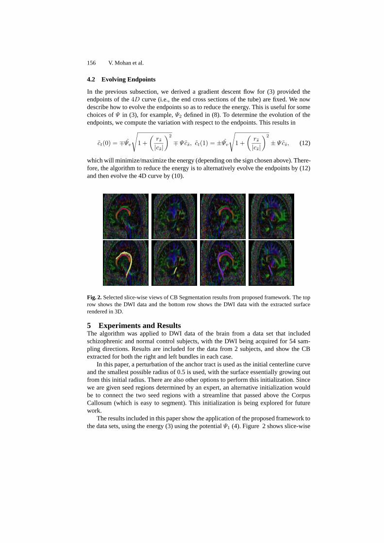
156 V. Mohan et al.
4.2 Evolving Endpoints
In the previous subsection, we derived a gradient descent flow for (3) provided theendpoints of the4D curve (i.e., the end cross sections of the tube) are fixed. We nowdescribe how to evolve the endpoints so as to reduce the energy. This is useful for somechoices ofΨ in (3), for example,Ψ2 defined in (8). To determine the evolution of theendpoints, we compute the variation with respect to the endpoints. This results in
ct(0) = ∓Ψv
√
1 +
(
rs
|cs|
)2
∓ Ψcs, ct(1) = ±Ψv
√
1 +
(
rs
|cs|
)2
± Ψcs, (12)
which will minimize/maximize the energy (depending on the sign chosen above). There-fore, the algorithm to reduce the energy is to alternativelyevolve the endpoints by (12)and then evolve the 4D curve by (10).
Fig. 2. Selected slice-wise views of CB Segmentation results from proposed framework. The toprow shows the DWI data and the bottom row shows the DWI data with the extracted surfacerendered in 3D.
5 Experiments and ResultsThe algorithm was applied to DWI data of the brain from a data set that includedschizophrenic and normal control subjects, with the DWI being acquired for 54 sam-pling directions. Results are included for the data from 2 subjects, and show the CBextracted for both the right and left bundles in each case.
In this paper, a perturbation of the anchor tract is used as the initial centerline curveand the smallest possible radius of 0.5 is used, with the surface essentially growing outfrom this initial radius. There are also other options to perform this initialization. Sincewe are given seed regions determined by an expert, an alternative initialization wouldbe to connect the two seed regions with a streamline that passed above the CorpusCallosum (which is easy to segment). This initialization isbeing explored for futurework.
The results included in this paper show the application of the proposed framework tothe data sets, using the energy (3) using the potentialΨ1 (4). Figure 2 shows slice-wise
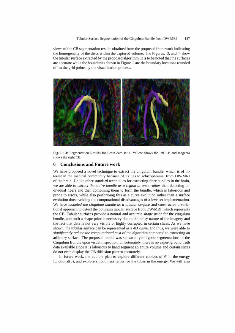
Tubular Surface Segmentation of the Cingulum Bundle from DW-MRI 157
views of the CB segmentation results obtained from the proposed framework indicatingthe homogeneity of the discs within the captured volume. TheFigures, 3, and 4 showthe tubular surface extracted by the proposed algorithm. Itis to be noted that the surfacesare accurate while the boundaries shown in Figure 2 are the boundary locations roundedoff to the grid points by the visualization process.
Fig. 3. CB Segmentation Results for Brain data set 1. Yellow shows the left CB and magentashows the right CB.
6 Conclusions and Future workWe have proposed a novel technique to extract the cingulum bundle, which is of in-terest in the medical community because of its ties to schizophrenia, from DW-MRIof the brain. Unlike other standard techniques for extracting fiber bundles in the brain,we are able toextract the entire bundle as a region at once ratherthan detecting in-dividual fibers and then combining them to form the bundle, which is laborious andprone to errors, while also performing this as a curve evolution rather than a surfaceevolution thus avoiding the computational disadvantages of a levelset implementation.We havemodeled the cingulum bundle as a tubular surfaceand constructed a varia-tional approach to detect the optimum tubular surface from DW-MRI, which representsthe CB. Tubular surfaces provide a natural and accurateshape priorfor the cingulumbundle, and such a shape prior is necessary due to the noisy nature of the imagery andthe fact that data is not very visible or highly corrupted in certain slices. As we haveshown, the tubular surface can be represented as a 4D curve, and thus, we were able tosignificantly reduce the computational costof the algorithm compared to extracting anarbitrary surface. The proposed model was shown to yield good segmentations of theCingulum Bundle upon visual inspection; unfortunately, there is no expert ground truthdata available since it is laborious to hand segment an entire volume and certain slicesdo not even display the CB diffusion pattern accurately.
In future work, the authors plan to explore different choices of Ψ in the energyfunctional(3), and explore smoothness terms for the tubes in the energy. We will also
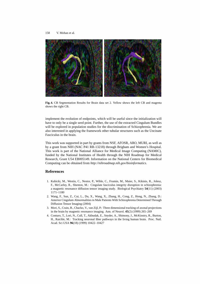
158 V. Mohan et al.
Fig. 4. CB Segmentation Results for Brain data set 2. Yellow shows the left CB and magentashows the right CB.
implement the evolution of endpoints, which will be useful since the initialization willhave to only be a single seed point. Further, the use of the extracted Cingulum Bundleswill be explored in population studies for the discrimination of Schizophrenia. We arealso interested in applying the framework other tubular structures such as the UncinateFasciculus in the brain.
This work was supported in part by grants from NSF, AFOSR, ARO, MURI, as well asby a grant from NIH (NAC P41 RR-13218) through Brigham and Women’s Hospital.This work is part of the National Alliance for Medical Image Computing (NAMIC),funded by the National Institutes of Health through the NIH Roadmap for MedicalResearch, Grant U54 EB005149. Information on the National Centers for BiomedicalComputing can be obtained fromhttp://nihroadmap.nih.gov/bioinformatics.
References
1. Kubicki, M., Westin, C., Nestor, P., Wible, C., Frumin, M., Maier, S., Kikinis, R., Jolesz,F., McCarley, R., Shenton, M.: Cingulate fasciculus integrity disruption inschizophrenia:a magnetic resonance diffusion tensor imaging study. Biological Psychiatry 54(11) (2003)1171–1180
2. Wang, F., Sun, Z., Cui, L., Du, X., Wang, X., Zhang, H., Cong,Z., Hong, N., Zhang, D.:Anterior Cingulum Abnormalities in Male Patients With Schizophrenia DeterminedThroughDiffusion Tensor Imaging (2004)
3. Mori, S., Crain, B., Chacko, V., van Zijl, P.: Three dimensional tracking of axonal projectionsin the brain by magnetic resonance imaging. Ann. of Neurol.45(2) (1999) 265–269
4. Conturo, T., Lori, N., Cull, T., Akbudak, E., Snyder, A., Shimony, J., McKinstry, R., Burton,H., Raichle, M.: Tracking neuronal fiber pathways in the living human brain. Proc. Natl.Acad. Sci USA96(18) (1999) 10422–10427
Tubular Surface Segmentation of the Cingulum Bundle from DW-MRI 159
5. Perrin, M., Poupon, C., Cointepas, Y., Rieul, B., Golestani, N., Pallier, C., Riviere, D., Con-stantinesco, A., Bihan, D.L., Mangin, J.F.: Fiber tracking in q-ball fields using regularizedparticle trajectories. [24] 52–63
6. Parker, G.J.M., Wheeler-Kingshott, C.A.M., Barker, G.J.: Estimating distributed anatomicalbrain connectivity using fast marching methods and diffusion tensor imaging. IEEE Trans.Med. Imaging21(5) (2002) 505–512
7. Friman, O., Farneback, G., Westin, C.F.: A bayesian approach for stochastic white mattertractography. IEEE Trans. Med. Imaging25(8) (2006) 965–978
8. Lenglet, C., Rousson, M., Deriche, R., Faugeras, O.D., Lehericy, S., Ugurbil, K.: A rieman-nian approach to diffusion tensor images segmentation. [24] 591–602
9. Control Theory and Fast Marching Techniques for Brain Connectivity Mapping. In: CVPR(1). (2006)
10. Zhang, F., Goodlett, C., Hancock, E.R., Gerig, G.: Probabilistic fiber tracking using particlefiltering. In Ayache, N., Ourselin, S., Maeder, A.J., eds.: MICCAI(2). Volume 4792 ofLecture Notes in Computer Science., Springer (2007) 144–152
11. Cohen-Adad, J., Descoteaux, M., Rossignol, S., Hoge, R.D.,Deriche, R., Benali, H.: De-tection of multiple pathways in the spinal cord white matter using q-ball imaging.In: IEEEInternational Symposium on Biomedical Imaging : From Nano to Macro. (2008)
12. Xu, C., Pham, D.L., Prince, J.L.: Finding the brain cortex using fuzzy segmentation, isosur-faces, and deformable surface models. In Duncan, J.S., Gindi, G., eds.: IPMI. Volume 1230of Lecture Notes in Computer Science., Springer (1997) 399–404
13. Yezzi, A.J., Kichenassamy, S., Kumar, A., Olver, P.J., Tannenbaum, A.: A geometric snakemodel for segmentation of medical imagery. IEEE Trans. Med. Imaging 16(2) (1997) 199–209
14. Lenglet, C., Rousson, M., Deriche, R.: Dti segmentation by statistical surface evolution.IEEE Trans. Med. Imaging25(6) (2006) 685–700
15. Wang, Z., Vemuri, B.C.: Dti segmentation using an information theoretic tensor dissimilaritymeasure. IEEE Trans. Med. Imaging24(10) (2005) 1267–1277
16. Awate, S.P., 0005, H.Z., Gee, J.C.: Fuzzy nonparametric dti segmentation for robustcingulum-tract extraction. In Ayache, N., Ourselin, S., Maeder, A.J., eds.: MICCAI (1).Volume 4791 of Lecture Notes in Computer Science., Springer (2007) 294–301
17. Melonakos, J., Mohan, V., Niethammer, M., Smith, K., Kubicki, M., Tannenbaum, A.:Finsler tractography for white matter connectivity analysis of the cingulum bundle. In: MIC-CAI (1). (2007) 36–43
18. Melonakos, J., Niethammer, M., Mohan, V., Smith, K., Kubicki, M., Tannenbaum, A.:Locally-constrained region-based methods for dw-mri segmentation.In: MMBIA. (2007)
19. Li, H., Yezzi, A.: Vessels as 4-d curves: Global minimal 4-d pathsto extract 3-d tubularsurfaces and centerlines. IEEE Transactions on Medical Imaging26(9) (2007) 1213–1223
20. Cohen, L.D., Kimmel, R.: Global minimum for active contour models: A minimal pathapproach. In: CVPR, IEEE Computer Society (1996) 666–673
21. Schmahmann, J., Pandya, D.: Fiber Pathways of the Brain. Oxford University Press (2006)22. Melonakos, J., Pichon, E., Angenent, S., Tannenbaum, A.: Finsler active contours. IEEE
Transactions on Pattern Analysis and Machine Intelligence (To Appear)23. Sundaramoorthi, G., Yezzi, A.J., Mennucci, A., Sapiro, G.: New possibilities with Sobolev
active contours. In: SSVM. (2007) 153–16424. Christensen, G.E., Sonka, M., eds.: Information Processing inMedical Imaging, 19th In-
ternational Conference, IPMI 2005, Glenwood Springs, CO, USA, July 10-15, 2005, Pro-ceedings. In Christensen, G.E., Sonka, M., eds.: IPMI. Volume 3565 of Lecture Notes inComputer Science., Springer (2005)
Modeling the Remaining Flexibility of PartiallyFixed Statistical Shape Models
Thomas Albrecht, Reinhard Knothe, and Thomas Vetter
Computer Science Department, University of Basel, SwitzerlandThomas.Albrecht,Reinhard.Knothe,[email protected]
Abstract. Statistical shape models are widely used to model the vari-ability of biological shapes. They can be used to reconstruct missinginformation given partial or noisy data. In case of partial data, manydifferent reconstructions are possible, and one is not only interested ina plausible reconstruction but also the remaining flexibility within themodel and the reliability of the reconstruction. We present a methodto model the remaining flexibility when some part of a statistical shapemodel is fixed. Using such a flexibility model, we can give answers toquestions like: Does one half of a human femur bone determine the otherhalf? or How much is the shape of a face determined by its contour?
1 Introduction
Statistical shape models are widely used in medical image analysis, computa-tional anatomy, and computer vision to model the variability of biological shapes,see [1–6] for instance. The variability of a certain class of shapes is deduced froma representative set of example data from this class.
If the example data sets represent the class of shapes well, the model can befitted to virtually any individual shape within the class. It is even possible tofit the model to partial data from an individual, [7, 8]. The missing remainingdata is automatically reconstructed by the model, yielding the most plausiblereconstruction.
However, there may be many other possible reconstructions which fit thepartial data equally well. The partial data only determines a part of the model,while the rest of the model may remain flexible. This paper focuses on modelingthis remaining flexibility of the partially determined model.
Keeping a part xb of the complete model x fixed, how much flexibility remainsfor the remaining part xa? In principle, as PCA models can be statistically inter-preted by a multivariate Gaussian distribution with probability density functionp, we can model the remaining flexibility by the conditional distribution p(xa|xb).We will see however, that there is no nontrivial conditional distribution if morecomponents are kept fixed than there are degrees of freedom in the model, as isusually the case in models built from a small set of examples.
In this case, we propose a method which models the remaining flexibility ofthe variable points when the fixed points are allowed to move slightly instead of
Flexibility of Shape Models 161
being completely fixed. The method leads to a generalized eigenvalue problemwhich can be solved efficiently.
The remaining paper is organized as follows. In Section 2 we will reviewthe well-known concept of PCA-based statistical shape models. In Section 3 wewill derive an expression of the conditional distribution p(xa|xb) and investigatewhen this can actually be used. In Section 4, we will model the remaining flexi-bility when the fixed points are allowed to move slightly. In Section 5 we will usethe proposed method to model the remaining flexibility of a shape model of thehuman femur bone when its distal part is fixed, and the remaining flexibility ofa face model, when its contour is fixed.
Related Work. Virtually all cited papers deal with statistical shape modelswith applications in medicine or computer vision, [1–8]. Most notably, [5] usesCanonical Correlation Analysis to model the correlation between different partsof a statistical model, computing model coefficients which maximize the correla-tion between these parts. However, they do not address our problem of modelingthe remaining flexibility when one part of the model is fixed.
2 Principle Component Analysis
The 3D statistical shape models used in this paper are based on a PrincipleComponent Analysis (PCA) of a set of training data comprised of n 3D surfaces.Each surface is represented by a triangular mesh with the same number m ∈ INof vertices, which are stacked into a data vector x = (x1, y1, z1, ...xm, ym, zm)T ∈IRM with M = 3m. The training surfaces need to be in correspondence.
As in all PCA models, the samples are assumed to be i.i.d. samples drawnfrom a multivariate normal distribution that is approximated by the estimatedmultivariate normal distribution N (x,Σ). The mean is estimated by the arith-metic mean x = 1
n
∑ni=1 xi of all samples. The covariance matrix Σ ∈ IRM×M
can be estimated from the mean-free data matrix X := [x1 − x, . . . ,xn − x] ∈IRM×n as Σ = 1
nXXT .When X is decomposed with a (reduced) Singular Value Decomposition
X = UWVT into the product of a column-orthonormal matrix U ∈ IRM×n,a diagonal matrix W ∈ IRn×n, and an orthonormal matrix V ∈ IRn×n, thecovariance matrix can be expressed as Σ = 1
nUW2UT .The columns ui of the matrix U are the eigenvectors of Σ. They are known
as the principal components of the model and describe the main modes of vari-ation of the training data. Their corresponding eigenvalues σ2
i := 1nw2
i describethe variance of the model projected onto these eigenvalues. They are arrangedaccording to size so that u1 is the direction with maximal projected variance σ2
1 .One individual x in the object class modeled by the PCA model can be
identified by its coefficients α = (α1, . . . , αn)T ∈ IRn:
x = x +n∑
i=1
αiσiui = x + 1√nUWα. (1)
162 Th. Albrecht et al.
Under the assumption that the data x is distributed according to a multivariatenormal distribution N (x,Σ), the coefficient vector α is distributed according toN (0, In).
In this paper two PCA models are used: A model of the femur bone, builtfrom 21 CT scans of femur bones, which were hand-segmented and brought intocorrespondence with [9], and a model of the human face built from 100 face scansthat were brought in correspondence with a modification of [10].
3 Conditional Distribution
In a PCA-based statistical model, we now wish to fix a certain number l ∈ IN ofpoints in the model in order to investigate how flexible the model remains withrespect to the remaining m − l variable points. This means that we fix L = 3lcomponents of the model vector x. Without loss of generality, we can assumethat they are the last l components and x can be partitioned as x = (xa,xb)T .
As x is distributed according to a multivariate normal distribution, the con-ditional distribution is a also a multivariate normal distribution N (µa|b,Σa|b).Its mean and covariance can be calculated from x and Σ.
The matrix of principal components U ∈ IRM×n can be partitioned accordingto x. For simplicity’s sake, we define the matrix of the principal componentsscaled by the diagonal matrix W ∈ IRn×n as Q := 1√
nUW ∈ IRM×n. We have
U =(Ua
Ub
), Q = 1√
nUW = 1√
n
(UaWUbW
)=
(Qa
Qb
)(2)
The covariance matrix Σ ∈ IRM×M can be calculated from Q by Σ =1nUW2UT = QQT . We can partition Σ as follows:
Σ =(Σaa Σab
Σba Σbb
)=
(QaQT
a QaQTb
QbQTa QbQT
b
). (3)
Note that it is only possible to calculate a nontrivial conditional distributionif the matrix Σbb is invertible. A necessary condition for Σbb to be invertibleis that the number of fixed degrees of freedom L is less the number of trainingexamples n of the statistical model. Let us, for the moment, assume that Σbb
is invertible and calculate the conditional distribution according. According to[11], the covariance matrix Σa|b of the can be expressed as:
Σa|b = Σaa −Σab Σ−1bb Σba (4)
= QaQTa −QaQT
b (QbQTb )−1 QbQT
a (5)
= Qa
(In −QT
b (QbQTb )−1Qb
)QT
a , (6)

Flexibility of Shape Models 163
where In denotes the (n × n) identity matrix. While the original matrix U iscolumn-orthonormal, the sub-matrix Ub defined in Equation (2) in not. There-fore, we perform an additional a singular value decomposition Qb = UbWbVT
b
with a column-orthonormal Ub. Thus, the expression can be expanded to:
Σa|b = Qa
(In −VbWbUT
b UbW−2b UT
b UbWbVb
)QT
a (7)
= Qa
(In −VT
b Vb
)QT
a . (8)
Where, in the last step, we have used UTb Ub = In. Similarly, the mean µa|b is
given as:
µa|b = xa + ΣabΣ−1bb (xb − xb) (9)
= xa + QaVbW−1b UT
b (xb − xb), (10)
with x = (xa, xb)T .Provided that Σbb is invertible, xa can be reconstructed from xb as µa|b. This
is the reconstruction presented in [7] as the maximum a posteriori reconstruction.All other reconstructions which fit xb are modeled by N (µa|b,Σa|b). The moreflexibility this distribution allows, the less reliable the reconstruction by µa|b is.
For each of these reconstructions, the fixed values xb are matched equallywell. Indeed, if we take a closer look at the expression for the covariance matrixΣa|b in Equation (8) we notice that the inner part (In −VT
b Vb) is a projectiononto the orthogonal complement of the column space of Vb. As Vb is the “inputmatrix” of the SVD of Qb, this projection is a projection onto the kernel of Qb.This means that the distribution N (µa|b,Σa|b) models only linear combinationsQaα of the scaled principal components for which α is in the kernel of Qb, i.e.Qbα = 0. So for all α ∼ N (µa|b,Σa|b), the deformation of the fixed points iszero.
Invertibility of Σbb. So far, we have assumed that Σbb = QbQTb ∈ IRL×L is in-
vertible, i.e. rank(Σbb) = L. However, if Qb has less than L linearly independentcolumns we have rank(Σbb) < L. In particular, if the statistical model is builtfrom less than L examples or less than L principal components are used, therank of Σbb will be less than L and the above calculations involving an inversionof Σbb are not valid. In this case there is no nontrivial conditional distributionp(xa,xb).
In this case the mean µa|b can still be approximated by using the pseudo-inverse of Σbb instead of its inverse, [7]. However, if we try to use the pseudo-inverse for calculating the covariance matrix according to Equation (4), we getΣa|b = 0.
The problem is that the conditional distribution N (µa|b,Σa|b) models onlycoefficient vectors from the kernel of Qb. Without a nontrivial kernel of Qb, itis not possible to calculate a nontrivial conditional distribution. Therefore, wepropose that instead of looking for coefficient vectors α ∈ kerQb, i.e. Qbα = 0,
164 Th. Albrecht et al.
we will look for coefficients for which Qbα is small. This means that we relaxthe constraint of keeping the fixed points completely fixed to allowing them tomove slightly.
It also has to be noted that even if there is a nontrivial kernel of Qb, it willmost likely still be of interest to consider deformations which allow slight changesof the fixed points xb when considering the remaining flexibility of the model.
4 Generalized Eigenvalues
The aim is to model the flexibility of the variable points xa when the fixed pointsxb are allowed to move slightly. The deformations are given as Qaα and Qbα. Ameasure for the change caused by these deformations is the squared Euclideannorm of these vectors:
‖Qaα‖2 = αT QTa Qaα, ‖Qbα‖2 = αT QT
b Qbα. (11)
As we are first and foremost interested in the coefficients α which change thevariable points xa as much as possible, we can formulate our aim as a constrainedmaximization problem:
maxα∈IRk
αT QTa Qaα (12)
subject to αT QTb Qbα = c, (13)
where c ∈ IR+ quantifies the amount of change allowed in the fixed coefficients.Introducing a Lagrangian multiplier λ and differentiating with respect to α
leads to the generalized eigenvalue problem:
QTa Qaα = λQT
b Qbα. (14)
Both matrices QTa Qa and QT
b Qb are positive definite and symmetric. The gen-eralized eigenvalue problem can be solved efficiently with standard software(LAPACK, MATLAB), yielding a set of generalized eigenvectors α1, . . . ,αkarranged according to the size of their corresponding generalized eigenvaluesλ1, . . . , λk. The eigenvectors are scaled so that ‖Qbαi‖2 = αT
i QTb Qbαi = 1
for i = 1, . . . , k. If we pre-multiply Equation (14) by αT , we see that for aneigenvector αi and its eigenvalue λi, we have
‖Qaαi‖2 = λi‖Qbαi‖2. (15)
This means that, measured in the squared Euclidean norm, the deformationdetermined by the coefficient vector αi ∈ IRk changes the variable model pointsλi times as much the fixed ones. Therefore, the eigenvector α1 corresponding tothe largest eigenvalue λ1 is the coefficient vector which causes the largest changeon the variable points (with a squared Euclidean norm of λ1), changing the fixedpoints only slightly (with a deformation with a squared Euclidean norm of 1).The last eigenvectors change the fixed points more than the variable ones. In

Flexibility of Shape Models 165
1st flexibility component mean 2nd flexibility component
−2.2√
l α1 +2.2√
l α1 0 −2.2√
l α2 +2.2√
l α2
Fig. 1. In a statistical shape model of the human femur bone, the two first flexibilitycomponents α1 and α2 model those deformations that change the proximal part (gray)as much as possible, while changing the distal part (colored) as little as possible.
fact, exchanging fixed and variable points leads to the same eigenvalues, onlyinverted.
We call the coefficient vectors αi the flexibility components. α1 is the firstflexibility component. Just like the principal components of the PCA model,they can be scaled and added together to achieve different deformations from themean. When a flexibility component αi is scaled by
√r it causes a deformation
of squared Euclidean norm r of the fixed points and of λi r of the variable points.The larger the eigenvalues λi are, the more flexibility remains for the fixed pointsand the less reliable a reconstruction of xa from xb is considered. In order tomeat the constraint from Equation (13), the vectors have to be scaled by
√c.
The squared Euclidean norm is not a very intuitive measure of the deforma-tion as it implicitly depends on the number l of fixed points. A more intuitivemeasure is the mean squared norm, averaged over all l fixed points:
1l
l∑k=1
(Qbαi)2k =1l‖Qbαi‖2. (16)
Therefore, if we scale the coefficient vectors αi by√
l, and the coordinates ofthe model are given in millimeters, the squared deformation of one model pointis 1 millimeter on average.
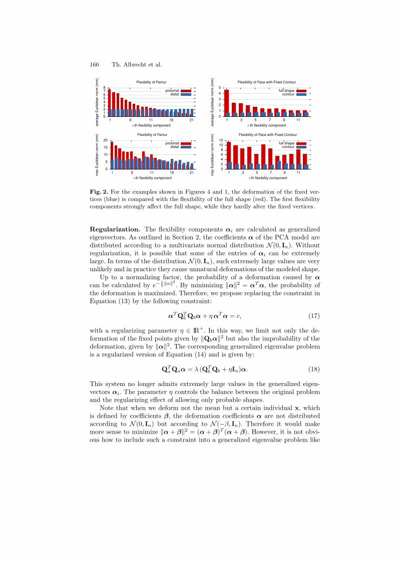
166 Th. Albrecht et al.
012345678
1 6 11 16 21
aver
age
Euc
lidea
nno
rm(m
m)
i-th flexibility component
Flexibility of Femur
proximaldistal
0
1
2
3
4
5
1 3 5 7 9 11
aver
age
Euc
lidea
nno
rm(m
m)
i-th flexibility component
Flexibility of Face with Fixed Contour
full shapecontour
0
5
10
15
20
1 6 11 16 21max
Euc
lidea
nno
rm(m
m)
i-th flexibility component
Flexibility of Femur
proximaldistal
02468
1012
1 3 5 7 9 11max
Euc
lidea
nno
rm(m
m)
i-th flexibility component
Flexibility of Face with Fixed Contour
full shapecontour
Fig. 2. For the examples shown in Figures 4 and 1, the deformation of the fixed ver-tices (blue) is compared with the flexibility of the full shape (red). The first flexibilitycomponents strongly affect the full shape, while they hardly alter the fixed vertices.
Regularization. The flexibility components αi are calculated as generalizedeigenvectors. As outlined in Section 2, the coefficients α of the PCA model aredistributed according to a multivariate normal distribution N (0, In). Withoutregularization, it is possible that some of the entries of αi can be extremelylarge. In terms of the distribution N (0, In), such extremely large values are veryunlikely and in practice they cause unnatural deformations of the modeled shape.
Up to a normalizing factor, the probability of a deformation caused by αcan be calculated by e−
12‖α‖
2. By minimizing ‖α‖2 = αT α, the probability of
the deformation is maximized. Therefore, we propose replacing the constraint inEquation (13) by the following constraint:
αT QTb Qbα + η αT α = c, (17)
with a regularizing parameter η ∈ IR+. In this way, we limit not only the de-formation of the fixed points given by ‖Qbα‖2 but also the improbability of thedeformation, given by ‖α‖2. The corresponding generalized eigenvalue problemis a regularized version of Equation (14) and is given by:
QTa Qaα = λ (QT
b Qb + ηIn)α. (18)
This system no longer admits extremely large values in the generalized eigen-vectors αi. The parameter η controls the balance between the original problemand the regularizing effect of allowing only probable shapes.
Note that when we deform not the mean but a certain individual x, whichis defined by coefficients β, the deformation coefficients α are not distributedaccording to N (0, In) but according to N (−β, In). Therefore it would makemore sense to minimize ‖α + β‖2 = (α + β)T (α + β). However, it is not obvi-ous how to include such a constraint into a generalized eigenvalue problem like
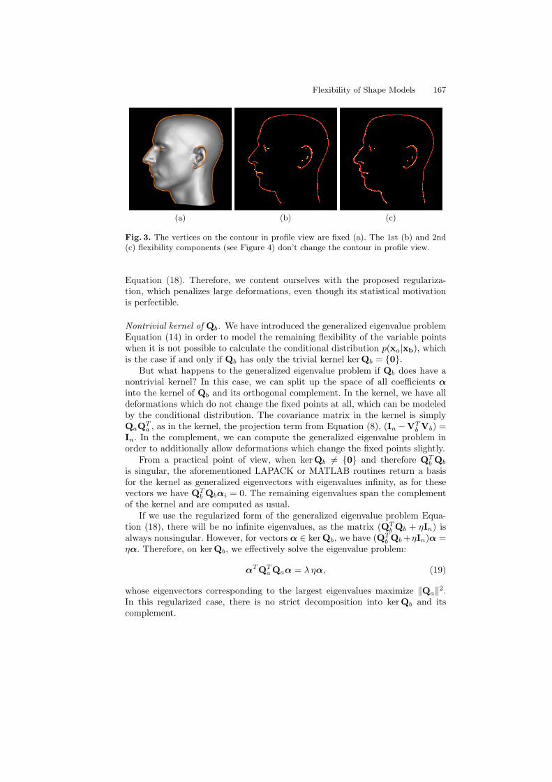
Flexibility of Shape Models 167
(a) (b) (c)
Fig. 3. The vertices on the contour in profile view are fixed (a). The 1st (b) and 2nd(c) flexibility components (see Figure 4) don’t change the contour in profile view.
Equation (18). Therefore, we content ourselves with the proposed regulariza-tion, which penalizes large deformations, even though its statistical motivationis perfectible.
Nontrivial kernel of Qb. We have introduced the generalized eigenvalue problemEquation (14) in order to model the remaining flexibility of the variable pointswhen it is not possible to calculate the conditional distribution p(xa|xb), whichis the case if and only if Qb has only the trivial kernel kerQb = 0.
But what happens to the generalized eigenvalue problem if Qb does have anontrivial kernel? In this case, we can split up the space of all coefficients αinto the kernel of Qb and its orthogonal complement. In the kernel, we have alldeformations which do not change the fixed points at all, which can be modeledby the conditional distribution. The covariance matrix in the kernel is simplyQaQT
a , as in the kernel, the projection term from Equation (8), (In −VTb Vb) =
In. In the complement, we can compute the generalized eigenvalue problem inorder to additionally allow deformations which change the fixed points slightly.
From a practical point of view, when kerQb 6= 0 and therefore QTb Qb
is singular, the aforementioned LAPACK or MATLAB routines return a basisfor the kernel as generalized eigenvectors with eigenvalues infinity, as for thesevectors we have QT
b Qbαi = 0. The remaining eigenvalues span the complementof the kernel and are computed as usual.
If we use the regularized form of the generalized eigenvalue problem Equa-tion (18), there will be no infinite eigenvalues, as the matrix (QT
b Qb + ηIn) isalways nonsingular. However, for vectors α ∈ kerQb, we have (QT
b Qb +ηIn)α =ηα. Therefore, on kerQb, we effectively solve the eigenvalue problem:
αT QTa Qaα = λ ηα, (19)
whose eigenvectors corresponding to the largest eigenvalues maximize ‖Qa‖2.In this regularized case, there is no strict decomposition into kerQb and itscomplement.
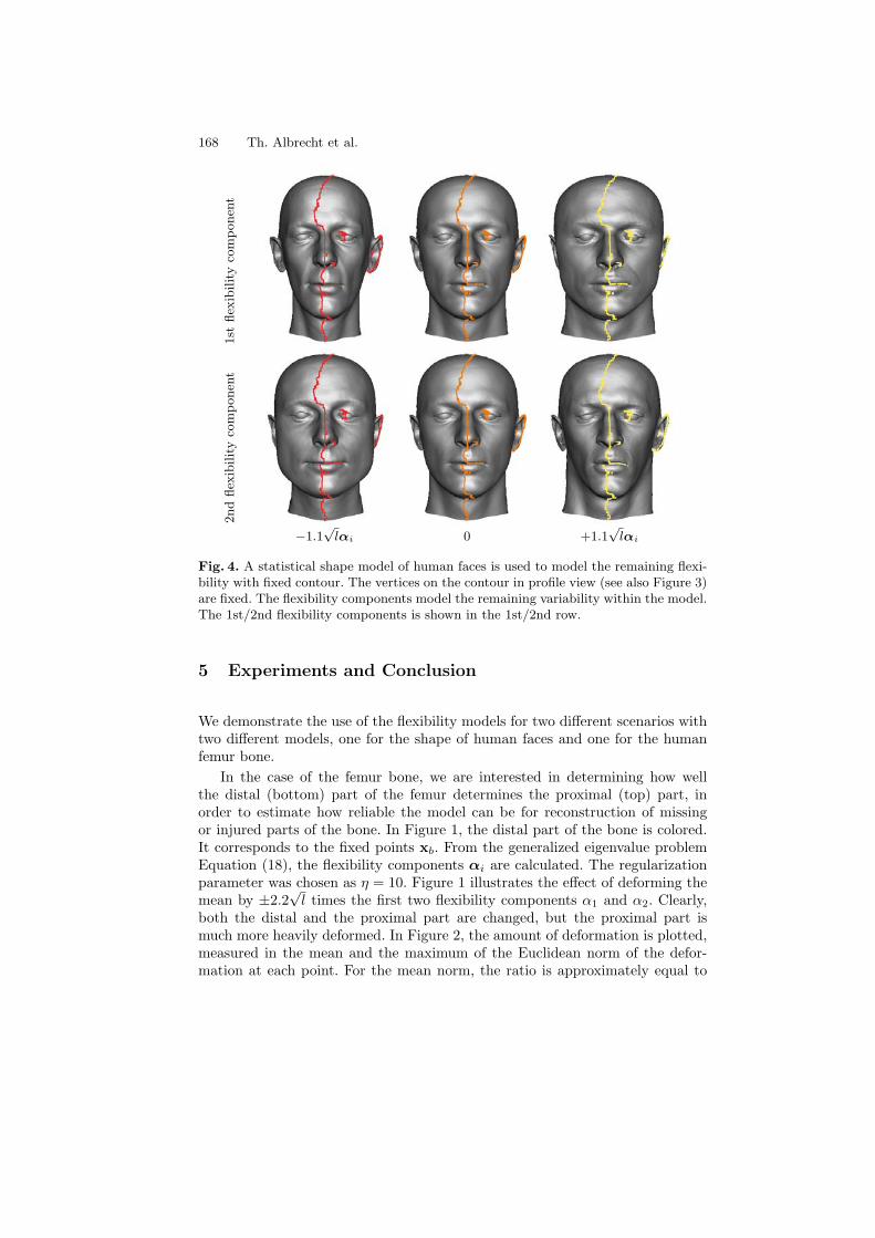
168 Th. Albrecht et al.
1st
flex
ibility
com
ponen
t2nd
flex
ibility
com
ponen
t
−1.1√
lαi 0 +1.1√
lαi
Fig. 4. A statistical shape model of human faces is used to model the remaining flexi-bility with fixed contour. The vertices on the contour in profile view (see also Figure 3)are fixed. The flexibility components model the remaining variability within the model.The 1st/2nd flexibility components is shown in the 1st/2nd row.
5 Experiments and Conclusion
We demonstrate the use of the flexibility models for two different scenarios withtwo different models, one for the shape of human faces and one for the humanfemur bone.
In the case of the femur bone, we are interested in determining how wellthe distal (bottom) part of the femur determines the proximal (top) part, inorder to estimate how reliable the model can be for reconstruction of missingor injured parts of the bone. In Figure 1, the distal part of the bone is colored.It corresponds to the fixed points xb. From the generalized eigenvalue problemEquation (18), the flexibility components αi are calculated. The regularizationparameter was chosen as η = 10. Figure 1 illustrates the effect of deforming themean by ±2.2
√l times the first two flexibility components α1 and α2. Clearly,
both the distal and the proximal part are changed, but the proximal part ismuch more heavily deformed. In Figure 2, the amount of deformation is plotted,measured in the mean and the maximum of the Euclidean norm of the defor-mation at each point. For the mean norm, the ratio is approximately equal to
Flexibility of Shape Models 169
the corresponding eigenvalue. For the mean squared norm, which is not plottedhere, it is of course exactly equal to this eigenvalue.
In case of the face model we are interested in the question: Given the verticeson the contour, how much is the shape of the face determined? Here, the fixedvertices xb are the vertices of the occluding contour in profile view, as shown inFigure (3 a)). This is the contour for one individual represented by its modelcoefficients β. Again, the flexibility components αi are computed using Equa-tion (18), with η = 10. To visualize the result, the surface with the coefficientsβ±1.1
√lαi is shown in Figure 4. We see that the first two flexibility components
heavily deform the model, while the vertices at the contour are almost fixed, seeFigure 3 b,c). The resulting deformations measures are plotted in Figure 2. Theratio is much higher than in the femur case as less points are kept fixed and themodel is built from many more examples, making it more expressive.
Conclusion. We have introduced a way to model the remaining flexibility of astatistical shape model when a part of the model is kept as fixed as possible,even in the absence of a nontrivial conditional distribution. In future work, wewill apply this technique in the fitting of statistical models to partial data.
References
1. Fleute, M., Lavallee, S.: Building a complete surface model from sparse data usingstatistical shape models: Application to computer assisted knee surgery. MedicalImage Computing and Computer-Assisted Intervention-MICCAI 98 880–7
2. Rajamani, K., Styner, M., Haydar, T., Nolte, L., Gonzalez Ballester, M.A.: Sta-tistical deformable bone models for robust 3d surface extrapolation from sparsedata. submitted to Elsevier Science (2006)
3. Subsol, G., Thirion, J., Ayache, N.: A scheme for automatically building three-dimensional morphometric anatomical atlases: application to a skull atlas. MedicalImage Analysis 2(1) (1998) 37–60
4. Dam, E., Fletcher, P., Pizer, S.: Automatic shape model building based on principalgeodesic analysis bootstrapping. Medical Image Analysis (2007)
5. Rao, A., Babalola, K., Rueckert, D.: Canonical Correlation Analysis of Sub-corticalBrain Structures Using Non-rigid Registration. Lecture Notes in Computer Science4057 (2006) 66
6. Shen, D., Herskovits, E., Davatzikos, C.: An adaptive-focus statistical shape modelfor segmentation and shape modeling of 3-D brain structures. IEEE Transactionson Medical Imaging 20(4) (2001) 257–270
7. Blanz, V., Vetter, T.: Reconstructing the complete 3d shape of faces from partialinformation. Informationstechnik und Technische Informatik 44(6) (2002) 1–8
8. Keller, M., Knothe, R., Vetter, T.: 3D Reconstruction of Human Faces from Oc-cluding Contours. Lecture Notes in Computer Science 4418 (2007) 261
9. Dedner, A., Luthi, M., Albrecht, T., Vetter, T.: Curvature guided level set regis-tration using adaptive finite elements. In: Pattern Recognition. (2007) 527–536
10. Amberg, B., Romdhani, S., Vetter, T.: Optimal Step Nonrigid ICP Algorithms forSurface Registration. Computer Vision and Pattern Recognition, 2007. CVPR’07.IEEE Conference on (2007) 1–8
11. Bishop, C.: Pattern recognition and machine learning. Springer (2006)
A Hypothesis Testing Framework forHigh-Dimensional Shape Models
Joshua Cates, P. Thomas Fletcher, Ross Whitaker
Scientific Computing and Imaging InstituteUniversity of Utah
Salt Lake City, Utah
Abstract. Statistical shape models are powerful tools for describinganatomical structures and are increasingly being used in a wide vari-ety of clinical and biological contexts. One of the promising applicationsof this technology is the testing of hypotheses that entail shape differ-ences, and visualization of those differences between cohorts. Statisticaltesting of shapes, however, is difficult due the large numbers of degreesof freedom and challenge of obtaining sufficient numbers of subjects toensure statistical power. To date, research in statistical shape modelinghas focused mainly on the construction of representative models, andthe field has not reached a consensus on the best approach to statisticalhypothesis testing. This paper illustrates some problems inherent in thestatistical analysis of high-dimensional shape models, and suggests a sys-tematic approach to hypothesis testing that avoids those problems. Theproposed framework is based on research in the factor analysis statis-tics literature, with permutation testing in the PCA space of the model,and dimensionality reduction via a a simulation-based analysis. We alsodescribe two methods for visualizing group mean differences, first by di-rect visualization of the linear discriminant implicit in the hypothesistest metric, and second, by visualizing strain tensors from a deformationcomputed between the group means. We illustrate the proposed analysisand visualization framework on several clinical and biological datasets.
1 Introduction
Many important fields of basic research in medicine and biology now routinelyemploy statistical models of shape to quantify the anatomical variation in popu-lations. Often, researchers are also interested in hypothesis testing to evaluate ordemonstrate shape differences between populations. One such application area,for example, is the study of gene function as it pertains to human developmentand disease. Modern gene targeting technology allows researchers to create spe-cific alterations in a mouse genome that result in different patterns of anatomicalgrowth and form, or phenotypes, which can be modeled as shape and comparedwith normal populations to gain insight into the functionality of the targetedgenes [1, 2]. Many areas of clinical psychiatric and neurological research alsoemploy statistical shape analysis. The study of autism and its impact on brain
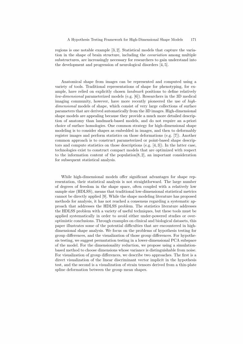
A Hypothesis Testing Framework for High-Dimensional Shape Models 171
regions is one notable example [3, 2]. Statistical models that capture the varia-tion in the shape of brain structure, including the covariation among multiplesubstructures, are increasingly necessary for researchers to gain understand intothe development and progression of neurological disorders [4, 5].
Anatomical shape from images can be represented and computed using avariety of tools. Traditional representations of shape for phenotyping, for ex-ample, have relied on explicitly chosen landmark positions to define relativelylow-dimensional parameterized models (e.g. [6]). Researchers in the 3D medicalimaging community, however, have more recently pioneered the use of high-dimensional models of shape, which consist of very large collections of surfaceparameters that are derived automatically from the 3D images. High-dimensionalshape models are appealing because they provide a much more detailed descrip-tion of anatomy than landmark-based models, and do not require an a-priorichoice of surface homologies. One common strategy for high-dimensional shapemodeling is to consider shapes as embedded in images, and then to deformablyregister images and perform statistics on those deformations (e.g. [7]). Anothercommon approach is to construct parameterized or point-based shape descrip-tors and compute statistics on those descriptions (e.g. [4, 3]). In the latter case,technologies exist to construct compact models that are optimized with respectto the information content of the population[8, 2], an important considerationfor subsequent statistical analysis.
While high-dimensional models offer significant advantages for shape rep-resentation, their statistical analysis is not straightforward. The large numberof degrees of freedom in the shape space, often coupled with a relatively lowsample size (HDLSS), means that traditional low-dimensional statistical metricscannot be directly applied [9]. While the shape modeling literature has proposedmethods for analysis, it has not reached a consensus regarding a systematic ap-proach that addresses the HDLSS problem. The statistics literature addressesthe HDLSS problem with a variety of useful techniques, but these tools must beapplied systematically in order to avoid either under-powered studies or over-optimistic conclusions. Through examples on clinical and biological datasets, thispaper illustrates some of the potential difficulties that are encountered in high-dimensional shape analysis. We focus on the problems of hypothesis testing forgroup differences, and the visualization of those group differences. For hypothe-sis testing, we suggest permutation testing in a lower-dimensional PCA subspaceof the model. For the dimensionality reduction, we propose using a simulation-based method to choose dimensions whose variance is distinguishable from noise.For visualization of group differences, we describe two approaches. The first is adirect visualization of the linear discriminant vector implicit in the hypothesistest, and the second is a visualization of strain tensors derived from a thin-platespline deformation between the group mean shapes.

172 J. Cates et al.
2 Related Work
Hypothesis testing for group differences using high-dimensional shape modelshas been most extensively investigated for comparative studies of brain anatomy.To date, however, researchers have typically each chosen different strategies foranalysis, and there has not been a systematic treatment of the effects of HDLSSand dimensionality reduction choices on the statistical tests. Davies, et al. inves-tigate hippocampus shape in schizophrenia populations with spherical harmonicand MDL-based shape models, and perform classification trials based on lineardiscriminant analysis in the high-dimensional shape space [8]. Terriberry [10] pro-poses a framework for multivariate, permutation-based hypothesis testing usingnonlinear m-rep shape models, with an application to the lateral ventricles oftwins. Styner, et al. propose point-wise hypothesis testing on shape correspon-dence points derived from spherical harmonic parameterizations [11, 12]. Golland[13] proposes a Support Vector Machine algorithm for training group classifiersof distance-transform shape representations. More recently, Gorczowski, et al.use medial axis shape representations and distance-weighted discriminants tocompare complexes of brain structures in autistic and normal populations [3].
Several researchers have explored hypothesis testing using high-dimensionalmodels for mouse phenotyping. Chen, et al. perform hypothesis testing usingimage-based metrics on deformation-based shape models to illustrate differencesbetween strains of mutant mice [7]. In a phenotyping study of Hoxd11 knock-outmice, the authors employ univariate hypothesis testing with regression analysison PCA bases of point-based models of the mouse forepaw [14].
3 Challenges for HDLSS Shape Statistics
This section describes some problems and solutions in HDLSS shape statistics asthey relate to shape analysis. The concepts presented here are applicable to lin-ear statistics using any high-dimensional model, though we will use surface-pointcorrespondence models as examples, computed by the particle-based optimiza-tion described in [2]. Point-based models represent shape by sampling each shapesurface in a consistently ordered fashion so as to define homologous object surfacepoints called correspondences. The set of 3D positions of all m correspondenceson a shape is 3m shape vector, and the positions of the individual shapes in this3m-dimensional shape space give rise to the statistical analysis. Hypothesis test-ing is done on a single shape model constructed from all data without knowledgeof the group classification, which we refer to as a combined model.
In the context of point-based models, or surface samplings obtained fromparameterized models, one approach to shape statistics is point-wise analysisof correspondences, which are elements of R3. These data are drawn from themarginal distributions of the full shape space, and the mean shape is obtained bycomputing the Euclidean averages of correspondence positions, with point-wisedifferences defining local shape variation [11]. Hypothesis tests in this case revealregions of significant differences between groups, which can be directly visualized
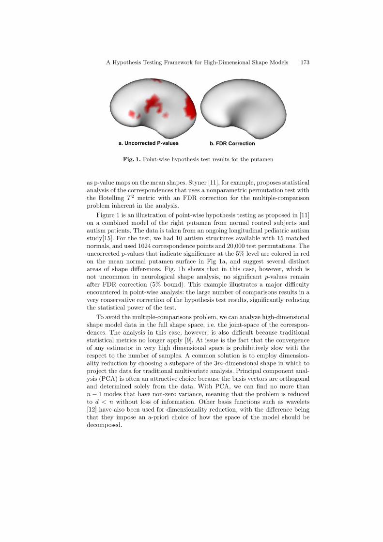
A Hypothesis Testing Framework for High-Dimensional Shape Models 173
a. Uncorrected P-values b. FDR Correction
Fig. 1. Point-wise hypothesis test results for the putamen
as p-value maps on the mean shapes. Styner [11], for example, proposes statisticalanalysis of the correspondences that uses a nonparametric permutation test withthe Hotelling T 2 metric with an FDR correction for the multiple-comparisonproblem inherent in the analysis.
Figure 1 is an illustration of point-wise hypothesis testing as proposed in [11]on a combined model of the right putamen from normal control subjects andautism patients. The data is taken from an ongoing longitudinal pediatric autismstudy[15]. For the test, we had 10 autism structures available with 15 matchednormals, and used 1024 correspondence points and 20,000 test permutations. Theuncorrected p-values that indicate significance at the 5% level are colored in redon the mean normal putamen surface in Fig 1a, and suggest several distinctareas of shape differences. Fig. 1b shows that in this case, however, which isnot uncommon in neurological shape analysis, no significant p-values remainafter FDR correction (5% bound). This example illustrates a major difficultyencountered in point-wise analysis: the large number of comparisons results in avery conservative correction of the hypothesis test results, significantly reducingthe statistical power of the test.
To avoid the multiple-comparisons problem, we can analyze high-dimensionalshape model data in the full shape space, i.e. the joint-space of the correspon-dences. The analysis in this case, however, is also difficult because traditionalstatistical metrics no longer apply [9]. At issue is the fact that the convergenceof any estimator in very high dimensional space is prohibitively slow with therespect to the number of samples. A common solution is to employ dimension-ality reduction by choosing a subspace of the 3m-dimensional shape in which toproject the data for traditional multivariate analysis. Principal component anal-ysis (PCA) is often an attractive choice because the basis vectors are orthogonaland determined solely from the data. With PCA, we can find no more thann− 1 modes that have non-zero variance, meaning that the problem is reducedto d < n without loss of information. Other basis functions such as wavelets[12] have also been used for dimensionality reduction, with the difference beingthat they impose an a-priori choice of how the space of the model should bedecomposed.

174 J. Cates et al.
5 10 15 20
0.00
0.05
0.10
0.15
0.20
0.25
0.30
Amygdala
Number of PCA Modes
P−
Val
ue
5 10 15 20
0.00
0.05
0.10
0.15
0.20
0.25
0.30
Putamen
Number of PCA Modes
P−
Val
ue
5 10 15 20
0.00
0.05
0.10
0.15
0.20
0.25
0.30
Hippocampus
Number of PCA Modes
P−
Val
ue
Fig. 2. Hotelling T 2 test results with increasing numbers of PCA modes for 3 brainstructures from a pediatric autism study.
In a suitably low-dimensional shape space, such as basis vectors from PCA,we can apply traditional statistical methods such as nonparametric Hotelling T 2
testing. There are two challenges for dimensionality reduction in shape analysis,however. First, is the the factor analysis problem of how many basis vectorsto choose, which can be hard to resolve when the choice of different numbersof factors leads to different statistical results. The second challenge is how tovisualize group differences, which is important for researchers in order to relatethe outcomes of statistical tests to scientific hypotheses regarding the growthand form of anatomy. The remainder of this section addresses the problem ofchoosing the number of bases, and then proposes two visualization strategies forunderstanding the group differences.
To illustrate the number-of-bases problem, Figure 2 shows the p-value resultsof Hotelling T 2 permutation tests using increasing numbers of PCA modes onthree brain structures from the pediatric autism study referenced above. Severaltrends can be observed that pose a challenge for the analysis. First, is the trendat higher numbers of modes towards increasing p-values, which is due to thecumulative effects of noise in the these lower-variance modes of the PCA. Thesecond trend is that the p-value curves do not smoothly decrease to a minimumvalue, but rather, tend to bounce around with lower numbers of higher-variancemodes. The challenge is to choose as many modes as possible that contain mean-ingful variation, i.e. variation that is distinguishable from noise, with the caveatthat too few modes may result in the loss of information that is useful for groupdiscrimination.
Many methodologies have been proposed to address the number-of-basesproblem, and good reviews such as [16], are available. Methodologies rangefrom simple conventions, such as choosing only PCA modes that account forat least 5% of the total variance, to more systematic approaches that attemptto model the problem based on its dimensionality and sample sizes. Notableamong these latter approaches, parallel analysis is commonly recommended asthe best method for determining modes with variance that is distinguishablefrom noise[17], and is described in more detail in Section 4.
A Hypothesis Testing Framework for High-Dimensional Shape Models 175
In contrast to the point-wise statistical method illustrated in Figure 1, asignificant drawback of hypothesis testing in a PCA subspace is that the groupdifferences in this space are not necessarily easy to visualize and interpret froman anatomical perspective. The hypothesis test poses the question of whetherthere are significant group differences. The next logical question of interest toresearchers is what are the group differences. One possible approach to gain in-sight into this question is to transform the group differences measured in thePCA space back into the full shape space, where they can be visualized on themean shape surfaces. Implicit in the Hotelling T 2 metric, for example, is a lin-ear discriminant which indicates the direction in the PCA space along whichthe maximum group difference is observed. This discriminant vector can be ro-tated back into the full shape space for visualization. Another standard approachfor visualizing group differences is a comparison of the differences in the meanshapes. Thin-plate spline analysis is commonly used in morphometric studies,for example, to visualize the deformations between shapes parameterized withlandmarks (sparse correspondences) [18], and a similar approach can be appliedin the context of high-dimensional point-based shape models. We discuss thesevisualization strategies further in the next section, along with the developmentof the dimensionality reduction and hypothesis testing.
4 Methodology
For a correspondence point shape model in 3D, we have a 3m× n shape matrixP, where columns of P are the shape vectors of correspondence points for theset of all samples. For dimensionality reduction, we first project P onto the basisvectors determined by PCA analysis, i.e. P = EP, where columns of E are theeigenvectors of the covariance matrix of correspondences, in decreasing order ofthe magnitude of their eigenvalues.
Following projection into the PCA space, we perform parallel analysis tochoose the number of PCA bases for hypothesis testing. In the context of princi-pal components analysis (PCA) of n, vector-valued data samples of dimension-ality 3m, the goal of parallel analysis is to identify the subset of the componentsthat contain variation distinguishable from the expected variation resulting fromnoise, where noise is modeled by an isotropic, multivariate unit Gaussian, i.e.a random 3m−vector X ∼ N (0, I). To make such a distinction, we need anestimator E for the expected values of the variances in the ordered PCA modesof random samplings from X, given the fixed sample size n. Due to the orderingproblem, there is no obvious closed-form expression for E, so it is estimatedusing Monte Carlo simulation. Many random sample sets of size n are indepen-dently drawn from X, followed by PCA on each sample set and ordering of theassociated eigenvalues. The ordered eigenvalues are then averaged to producean estimate of the Gaussian noise variance profile across modes. Note that theeigenvalues in this case quantify variance, and the percentage of total variancefor a PCA mode is equivalent to the ratio of its eigenvalue to the sum of alleigenvalues.
176 J. Cates et al.
In order to determine the number of modes to use from parallel analysis, thepercent-total-variance profiles from the Monte Carlo simulation and the PCA ofthe true data are compared, and only modes where the percent-total-variancein the true data is greater than the simulation data are retained. Figure 3, forexample, is a scree plot of the percent-variances associated with shape data of aputamen brain structure (n = 25, 3m = 3000) [19] (solid line) and the variancesfrom the Monte Carlo noise variance simulation (dashed line). The two linesintersect just before mode 6, and so we would consider only modes 1-5 in theanalysis.
5 10 15 20
0.00
0.05
0.10
0.15
0.20
0.25
0.30
Number of PCA Modes
Per
cent
of T
otal
Var
ianc
e
Fig. 3. Parallel analysis for the putamen data
Once we have chosen the set of k PCA basis vectors by parallel analysis,we project the correspondences into that subspace. Hypothesis testing for groupdifferences can now be done using a nonparametric, permutation test with theHotelling T 2 metric, with the null hypothesis that the two groups are drawnfrom the same distribution.
The Hotelling T 2, two-sample metric is given by
T 2 =(nanb)(na + nb − 2)
na + nb(µa − µb)T w,
w = (Σa + Σb)−1(µa − µb)(1)
where µa and µb are the means, Σa and Σb are the covariances, and na and nb
are the sample sizes of the two groups, respectively. Note that the vector w is alsoFisher’s linear discriminant, which is well known to be the line along which thebetween-group variance is maximized with respect to within-group variance[20].The Hotelling T 2 metric is therefore a scaled projection of the group differenceonto the discriminant line. We therefore propose to visualize the morphologicaldifferences that are driving the statistical test results by transforming w backfrom PCA space into the full-dimensional shape space, i.e. w = E−1w, where w
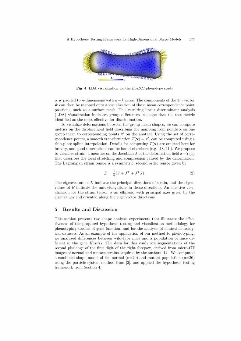
A Hypothesis Testing Framework for High-Dimensional Shape Models 177
0+-
Fig. 4. LDA visualization for the HoxD11 phenotype study
is w padded to n-dimensions with n−k zeros. The components of the 3m vectorw can then be mapped onto a visualization of the n mean correspondence pointpositions, such as a surface mesh. This resulting linear discriminant analysis(LDA) visualization indicates group differences in shape that the test metricidentified as the most effective for discrimination.
To visualize deformations between the group mean shapes, we can computemetrics on the displacement field describing the mapping from points x on onegroup mean to corresponding points x′ on the another. Using the set of corre-spondence points, a smooth transformation T (x) = x′, can be computed using athin-plate spline interpolation. Details for computing T (x) are omitted here forbrevity, and good descriptions can be found elsewhere (e.g. [18, 21]). We proposeto visualize strain, a measure on the Jacobian J of the deformation field x−T (x)that describes the local stretching and compression caused by the deformation.The Lagrangian strain tensor is a symmetric, second order tensor given by
E =12(J + JT + JT J). (2)
The eigenvectors of E indicate the principal directions of strain, and the eigen-values of E indicate the unit elongations in those directions. An effective visu-alization for the strain tensor is an ellipsoid with principal axes given by theeigenvalues and oriented along the eigenvector directions.
5 Results and Discussion
This section presents two shape analysis experiments that illustrate the effec-tiveness of the proposed hypothesis testing and visualization methodology forphenotyping studies of gene function, and for the analysis of clinical neurolog-ical datasets. As an example of the application of our method to phenotyping,we analyzed differences between wild-type mice and a population of mice de-ficient in the gene Hoxd11. The data for this study are segmentations of thesecond phalange of the first digit of the right forepaw, derived from micro-CTimages of normal and mutant strains acquired by the authors [14]. We computeda combined shape model of the normal (n=20) and mutant population (n=20)using the particle system method from [2], and applied the hypothesis testingframework from Section 4.
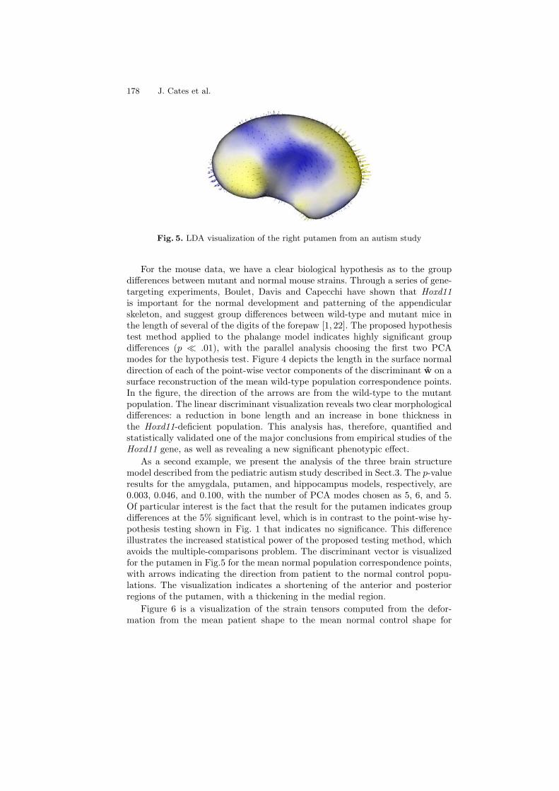
178 J. Cates et al.
Fig. 5. LDA visualization of the right putamen from an autism study
For the mouse data, we have a clear biological hypothesis as to the groupdifferences between mutant and normal mouse strains. Through a series of gene-targeting experiments, Boulet, Davis and Capecchi have shown that Hoxd11is important for the normal development and patterning of the appendicularskeleton, and suggest group differences between wild-type and mutant mice inthe length of several of the digits of the forepaw [1, 22]. The proposed hypothesistest method applied to the phalange model indicates highly significant groupdifferences (p .01), with the parallel analysis choosing the first two PCAmodes for the hypothesis test. Figure 4 depicts the length in the surface normaldirection of each of the point-wise vector components of the discriminant w on asurface reconstruction of the mean wild-type population correspondence points.In the figure, the direction of the arrows are from the wild-type to the mutantpopulation. The linear discriminant visualization reveals two clear morphologicaldifferences: a reduction in bone length and an increase in bone thickness inthe Hoxd11-deficient population. This analysis has, therefore, quantified andstatistically validated one of the major conclusions from empirical studies of theHoxd11 gene, as well as revealing a new significant phenotypic effect.
As a second example, we present the analysis of the three brain structuremodel described from the pediatric autism study described in Sect.3. The p-valueresults for the amygdala, putamen, and hippocampus models, respectively, are0.003, 0.046, and 0.100, with the number of PCA modes chosen as 5, 6, and 5.Of particular interest is the fact that the result for the putamen indicates groupdifferences at the 5% significant level, which is in contrast to the point-wise hy-pothesis testing shown in Fig. 1 that indicates no significance. This differenceillustrates the increased statistical power of the proposed testing method, whichavoids the multiple-comparisons problem. The discriminant vector is visualizedfor the putamen in Fig.5 for the mean normal population correspondence points,with arrows indicating the direction from patient to the normal control popu-lations. The visualization indicates a shortening of the anterior and posteriorregions of the putamen, with a thickening in the medial region.
Figure 6 is a visualization of the strain tensors computed from the defor-mation from the mean patient shape to the mean normal control shape for

A Hypothesis Testing Framework for High-Dimensional Shape Models 179
0+-
Fig. 6. Strain tensors for the right putamen from an autism study. Tensor scale isexaggerated for visualization.
the putamen data. The strain tensors were computed from a thin-plate splinedeformation, as described in the previous section. In the figure, the three prin-cipal axes of each ellipsoid are scaled by the three principal eigenvalues of thestrain tensor at each correspondence position, and oriented according to theircorresponding eigenvectors. Ellipsoids and the surrounding surface are coloredaccording to the value of the first principal eigenvector (the longest axis), withyellow indicating negative (compression) and blue indicating positive (stretch-ing). While a clinical interpretation of this result is beyond the scope of thispaper, this visualization clearly offers a more detailed insight into how groupsdiffer than, for example, the LDA visualization. Note, however, that that in thiscase we have no indication of the statistical significance of these differences.
In summary, the proposed hypothesis testing and visualization methodolo-gies offer an intuitive approach to analysis of anatomical shape from imagesfor biological and clinical research, and avoid the problems inherent in HDLSSstatistics. We have illustrated the effectiveness of the framework by statisticallyvalidating a biological hypothesis regarding Hoxd11 gene function that was pre-viously only based on empirical evidence, and we have shown how the methodcan be useful in exploring new patterns in shape from clinical data which havenot previously been observed, or that are not observable with lower-poweredstatistical methods.
Acknowledgments
This work was funded by the Center for Integrative Biomedical Computing, Na-tional Institutes of Health (NIH) NCRR Project 2-P41-RR12553-07. This workis also part of the National Alliance for Medical Image Computing (NAMIC),funded by the National Institutes of Health through the NIH Roadmap for Med-ical Research, Grant U54 EB005149.
180 J. Cates et al.
References
1. Davis, A., Capecchi, M.: Axial homeosis and appendicular skeleton defects in micewith targeted disruption of hoxd-11. Development 120 (1995) 2187–2198
2. Cates, J., Fletcher, P.T., Styner, M., Shenton, M., Whitaker, R.: Shape modelingand analysis with entropy-based particle systems. In: Information Processing inMedical Imaging (IPMI 2007), LNCS 4584. (2007) 333–345
3. Gorczowski, K., Styner, M., Jeong, J., Marron, J., Piven, J., Hazlett, H., Pizer, S.,Gerig, G.: Statistical shape analysis of multi-object complexes. In: Proceedings ofIEEE Conference on Computer Vision and Pattern Recognition, IEEE (2007) 1–8
4. Styner, M., Lieberman, J.A., Pantazis, D., Gerig, G.: Boundary and medial shapeanalysis of the hippocampus in schizophrenia. Medical Image Analysis (2004)
5. Pizer, S.M., Jeong, J.Y., Lu, C., Muller, K.E., Joshi, S.C.: Estimating the statis-tics of multi-object anatomic geometry using inter-object relationships. In: DeepStructure, Singularities, and Computer Vision. Volume 3753 of LNCS. (2005) 60–71
6. Klingenberg, C.P.: Morphometrics and the role of the phenotype in studies of theevolution of developmental mechanisms. Gene 287 (2002) 3–10
7. Chen, X.J., Kovacevic, N., Lobaugh, N.J., Sled, J.G., Henkelman, R.M., Hender-son, J.T.: Neuroanatomical differences between mouse strains as shown by high-resolution 3d mri. NeuroImage 29 (2005) 99–105
8. Davies, R.H., Twining, C.J., Allen, P.D., Cootes, T.F., Taylor, C.J.: Shape dis-crimination in the hippocampus using an mdl model. In: IPMI. (2003) 38–50
9. Ahn, J., Marron, J.S., Muller, K.M., Chi, Y.: The high-dimension, low-sample-sizegeometric representation holds under mild conditions. Biometrika 94(3) (2007)760–766
10. Terriberry, T., Joshi, S., Gerig, G.: Hypothesis testing with nonlinear shape models.In: IPMI’05. (2005) 15–26
11. Styner, M., Oguz, I., Xu, S., Brechbuhler, C., Pantazis, D., Levitt, J., Shenton, M.,Gerig, G.: Framework for the statistical shape analysis of brain structures usingSPHARM-PDM. The Insight Journal (2006)
12. Nain, D., Niethammer, M., Levitt, J., Shenton, M., Gerig, G., Bobick, A., Tannen-baum, A.: Statistical shape analysis of brain structures using spherical wavelets.In: IEEE Symposium on Biomedical Imaging ISBI. (2007) in print
13. Golland, P., Grimson, W., Shenton, M., Kikinis, R.: Detection and analysis ofstatistical differences in anatomical shape. Medical Image Analysis 9 (2005) 69–86
14. Cates, J., Fletcher, P.T., Warnock, Z., Whitaker, R.: A shape analysis frameworkfor small animal phenotyping with application to mice with a targeted disruptionof hoxd11. In: Proc. 5th IEEE International Symposium on Biomedical Imaging(ISBI ’08). (2008) 512–516
15. Hazlett, H., Poe, M., Gerig, G., Smith, R., Provenzale, J., Ross, A., Gilmore, J.,Piven, J.: Magnetic resonance imaging and head circumference study of brain sizein autism: Birth through age 2 years. Arch Gen Psych 62 (2005) 1366–1376
16. Fabrigar, L.R., Wegener, D.T., MacCallum, R.C., Strahan, E.J.: Evaluating theuse of exploratory factor analysis in psychological research. Psychological Methods4 (1999) 272–299
17. Glorfeld, L.W.: An improvement on horn’s parallel analysis methodology for se-lecting the correct number of factors to retain. Educational and PsychologicalMeasurement 55 (1995) 377–393
18. Bookstein, F.: Principal warps: Thin plate splines and the decomposition of defor-mations. IEEE Transactions on Pattern Analysis and Machine Intelligence 11(6)(1989)

A Hypothesis Testing Framework for High-Dimensional Shape Models 181
19. Cates, J., Fletcher, P., Styner, M., Hazlett, H., Whitaker, R.: Particle-based shapeanalysis of multi-object complexes. In: Proceedings of the 11th International Con-ference on Medical Image Computing and Computer Assisted Intervention, MIC-CAI (2008) to appear
20. Timm, N.H.: Applied Multivariate Analysis. Springer-Verlag (2002)21. Whitbeck, M., Guo, H.: Multiple landmark warping using thin-plate splines. In:
IPCV. (2006) 256–26322. Boulet, A.M., Capecchi, M.R.: Duplication of the hoxd11 gene causes alterations
in the axial and appendicular skeleton of the mouse. Developmental Biology 249(2002) 96–107

Author Index
Albrecht, Th., 160Allassonniere, S., 80Ayache, N., 68
Barysheva, M., 48Bigot, J., 92Bossa, M., 13Brun, C., 48
Cahill, N.D., 117Cates, J., 170Chan, T., 36, 56Chou, Y.Y., 48Chung, M.K., 128
Davidson, R.J., 128Durrleman, S., 68
Fletcher, P.T., 170
Gorelick, L., 117Gu, X., 36Gutman, B., 56
Hernandez, M., 24
Kim, P.T., 140Knothe, R., 160Kubicki, M., 150Kuhn, E., 80
Le Guyader, C., 1Lee, A., 48Leow, A., 1Lepore, N., 48Liu, X., 105Loubes, J.-M., 92
McMahon, K.L., 48Melonakos, J., 150
Meredith, M., 48Mio, W., 105Mohan, V., 150
Nacewicz, B.M., 128Niethammer, M., 150Noble, J.A., 117
Olmos, S., 13, 24
Pennec, X., 24, 68Pollak, S., 128
Qiu, A., 128
Richards, D.St.P., 140
Shi, Y., 105Sundaramoorthi, G., 150
Tannnenbaum, A., 150Thompson, P.M., 1, 36, 48, 56Toga, A.W., 1, 48, 56Trouve, A., 68, 80
Vese, L., 1Vesom, G., 117Vetter, Th., 160Vimond, M., 92
Wang, Y., 36, 56Whitaker, R., 170Wright, M.J., 48
Yanovsky, I., 1Yau, S.T., 36Yin, X., 36
Zhang, J., 36Zubicaray (de), G.I., 48