Research Division Federal Reserve Bank of St. Louis Working Paper Series

Metro Business Cycles

Maria A. Arias Charles S. Gascon

and David E. Rapach

Working Paper 2014-046C

http://research.stlouisfed.org/wp/2014/2014-046.pdf

November 2014 Revised May 2016

FEDERAL RESERVE BANK OF ST. LOUIS

Research Division P.O. Box 442

St. Louis, MO 63166

______________________________________________________________________________________

The views expressed are those of the individual authors and do not necessarily reflect official positions of the Federal Reserve Bank of St. Louis, the Federal Reserve System, or the Board of Governors.

Federal Reserve Bank of St. Louis Working Papers are preliminary materials circulated to stimulate discussion and critical comment. References in publications to Federal Reserve Bank of St. Louis Working Papers (other than an acknowledgment that the writer has had access to unpublished material) should be cleared with the author or authors.

Metro Business Cycles

Maria A. Arias

Federal Reserve Bank of St. Louismaria.a.arias@stls.frb.org

Charles S. Gascon

Federal Reserve Bank of St. Louischarles.s.gascon@stls.frb.org

David E. Rapach

⇤

Saint Louis Universityrapachde@slu.edu

May 9, 2016

⇤Corresponding author. Send correspondence to David E. Rapach, Department of Economics, JohnCook School of Business, Saint Louis University, 3674 Lindell Boulevard, St. Louis, MO 63108; e-mail:rapachde@slu.edu; phone: 314-977-3601. The views expressed in this paper are those of the authors and donot reflect those of the Federal Reserve Bank of St. Louis or the Federal Reserve System.

Metro Business Cycles

Abstract

We construct monthly economic activity indices for the 50 largest U.S. metropolitanstatistical areas (MSAs) beginning in 1990. Each index is derived from a dynamicfactor model based on twelve underlying variables capturing various aspects of metroarea economic activity. To accommodate mixed-frequency data and di↵erences indata-publication lags, we estimate the dynamic factor model using a maximum-likelihood approach that allows for arbitrary patterns of missing data. Our indiceshighlight important similarities and di↵erences in business cycles across MSAs. Whilea number of MSAs experience sizable recessions during the national recessions of theearly 1990s and early 2000s, other MSAs escape recessions altogether during one or bothof these periods. Nearly all MSAs su↵er relatively deep recessions near the recent GreatRecession, but we still find significant di↵erences in the depth of recent metro recessions.We relate the severity of metro recessions to a variety of MSA characteristics and findthat MSAs with less-educated populations and less elastic housing supplies experiencesignificantly more severe recessions. After controlling for national economic activity,we also find significant evidence of dynamic spillover e↵ects in economic activity acrossMSAs.

JEL classifications: C38, E32, R11, R31

Keywords: Economic activity index; Metropolitan statistical area; Recession; Dynamicfactor model; Latent variable; EM algorithm; Mixed regressive, spatial autoregressivemodel; Dynamic spillovers

1. Introduction

The grand tradition of Burns and Mitchell (1946) views business cycles as common

fluctuations in a host of economic variables. Beginning with Geweke (1977) and Sargent

and Sims (1977), and continuing with Stock and Watson (1989, 1991), researchers have

formalized this notion by developing dynamic factor models that allow for the estimation

of a latent common factor—an index of economic activity—underlying the comovements in

multiple variables. For example, Stock and Watson (1989, 1991) specify a dynamic factor

model for four national variables (industrial production, personal income, manufacturing

and retail sales, and employment) to estimate a monthly economic activity index for the

United States. Subsequently, a sizable literature uses dynamic factor models to construct

economic activity indices for the United States and other countries based on a larger number

of individual economic variables; see, for example, Arouba et al. (2009) for the Unites States

and Altissimo et al. (2001) for the Euro area.1

Although the bulk of the literature focuses on national activity indices, a few studies

construct monthly indices for individual U.S. states. For example, adopting the approach of

Stock and Watson (1989, 1991), Crone and Clayton-Matthews (2005) estimate an economic

activity index for each of the 50 individual U.S. states using a dynamic factor model and

four state-level labor-market variables (payroll employment, the unemployment rate, average

hours worked in manufacturing, and real wage and salary disbursements), while Bram

et al. (2009) develop indices for New York and New Jersey using a similar approach.2

State indices allow researchers to compare state business cycles to the national cycle (e.g.,

Owyang et al., 2005; Crone, 2006) and to link di↵erences in state business cycles to state

characteristics (e.g., Owyang et al., 2009). Along the lines of Wall and Zoega (2002)

1Marcellino (2006) and Stock and Watson (2011) provide extensive surveys of dynamic factor models.2Indices based on these studies are reported regularly by the Federal Reserve Banks of Philadelphia

(available at http://www.philadelphiafed.org/research-and-data/regional-economy/indexes/coincident/)and New York (available at http://www.ny.frb.org/research/regional economy/coincident summary.html),respectively.

1

and Nakamura and Steinsson (2014), they also provide researchers with more information

for estimating economic relations that are typically estimated using national data. Of

course, state indices supply state governments with important information for formulating

appropriate policies in light of economic conditions, and state indices also inform national

policymakers of regional di↵erences in economic conditions when setting national economic

policies.3

While national and state indices of monthly economic activity are now widely available,

monthly economic activity indices are currently only available for a small number of U.S.

metropolitan statistical areas (MSAs), despite their potential value. Metro indices allow

for an even more disaggregated geographical comparison of business cycles, thus permitting

researchers to identify significant di↵erences in economic activity that are masked by existing

state indices. In this vein—and similarly to Ghent and Owyang (2010), Mian et al. (2013),

Kiley (2014), and Mian and Sufi (2014)—metro indices provide a rich source of variation

in economic activity that can be exploited to analyze important economic relations with

greater precision. Metro indices are also clearly valuable to local governments for setting

policy, and they provide state and national governments with a more complete picture of

di↵erences in local economic activity when deciding on appropriate policies at the state and

national levels, respectively.

In this paper, we develop monthly economic activity indices for the 50 largest MSAs (by

population) in the United States.4 In the spirit of Burns and Mitchell (1946), our goal is to

measure economic activity by incorporating information from a wide array of metro variables.

Data issues, however, present keen challenges for achieving this goal; most pressingly, we

need to accommodate mixed-frequency data, di↵erent starting dates for some variables, and

di↵erent publication lags across variables. To this end, we construct each metro index via

a dynamic factor model based on twelve underlying metro variables, where we estimate the

3Regional economic conditions appear relevant for the Federal Reserve’s monetary policy decisions, asexemplified by the Beige Book.

4Table 1 provides a complete list of the 50 largest MSAs and their populations in 2014.

2

model using the recently developed maximum-likelihood approach of Banbura and Modugno

(2014). Their approach relies on the Expectation Maximization (EM) algorithm of Dempster

et al. (1977) to implement maximum-likelihood estimation and is explicitly designed to

handle arbitrary patterns of missing data, including mixed-frequency data and missing data

for some variables at the beginning and/or end of the sample. The Banbura and Modugno

(2014) procedure allows us to compute monthly metro economic activity indices based on a

large number of local variables in a timely manner.

To the best of our knowledge, the only extant monthly economic activity indices at the

MSA level are for New York City and nine MSAs in Texas, which are produced by the Federal

Reserve Banks of New York and Dallas, respectively.5 The New York City index is based

on four labor-market variables, while the indices for the Texas MSAs are based on three

labor-market variables and retail sales. Our study is thus the first to construct consistent

monthly economic activity indices based on a broad array of local economic variables for a

large number of U.S. metro areas.

We calibrate our monthly metro indices to annual gross metropolitan product (GMP)

growth. This strategy is analogous to Clayton-Matthews and Stock (1998), who calibrate

an economic activity index for Massachusetts to gross state product (GSP) growth. By

calibrating our metro indices to GMP growth, we create economically meaningful scales,

so that we can compare business-cycle fluctuations across MSAs. In conjunction with a

nonparametric algorithm, our indices’ meaningful scales allow us to identify a complete set

of monthly business-cycle peaks and troughs for the 50 MSAs.

Our economic activity indices reveal important similarities and di↵erences in business

cycles across MSAs. Important di↵erences are evident around the national recessions of

the early 1990s and early 2000s. Although many MSAs experience sizable recessions during

these periods, others manage to escape recessions altogether during one or both of these

periods. Indeed, we even find marked di↵erences in business cycles across MSAs within the

5Available at http://www.newyorkfed.org/research/regional economy/coincident summary.html andhttp://www.dallasfed.org/research/econdata/mbci.cfm, respectively.

3

same state. For example, San Jose and San Francisco endure deep recessions during the early

2000s, while Riverside, San Diego, and Sacramento do not experience recessions at all during

this period. There are greater similarities across MSAs near the recent Great Recession, as

nearly all MSAs su↵er relatively deep recessions in the late 2000s. Nevertheless, our indices

still indicate substantive di↵erences in the depth of recent recessions across some MSAs.

To gain insight into the underlying sources of di↵erences in business-cycle fluctuations

across MSAs, we relate the severity of metro recessions to a variety of MSA characteristics.

We present robust cross-sectional evidence that MSAs with less-educated populations and

less elastic housing supplies experience more severe recessions. The negative relation between

housing supply elasticity and recession severity across MSAs lines up well with recent findings

reported in Glaeser et al. (2008), Mian et al. (2013), and Mian and Sufi (2014). The

first study finds that areas with lower housing supply elasticities are more susceptible to

“boom-bust” housing cycles, while the latter two studies detect large consumption responses

to housing net worth shocks. In conjunction, these studies indicate that areas with less

elastic housing supply are more likely to su↵er large declines in housing net worth and sharp

concomitant decreases in consumption spending, making areas with inelastic housing supply

more vulnerable to recessions. Our results confirm that such a pattern exists across MSAs.

In the context of a mixed regressive, spatial autoregressive (MRSAR) model, we also detect

significant spatial e↵ects in the severity of metro recessions.

Finally, we test for dynamic spillover e↵ects using the infinite-dimensional vector

autoregression (IVAR) approach and cross-section augmented least squares (CALS)

estimation procedure recently developed by Chudik and Pesaran (2011). Their methodology

allows us to parsimoniously estimate dynamic spillovers between MSAs, while controlling

for national economic activity. The CALS estimation results provide significant evidence of

dynamic spillover e↵ects across a number of MSAs.

The rest of the paper is organized as follows. Section 2 specifies the dynamic factor model

and outlines maximum-likelihood estimation of the model. Section 3 describes the MSA data

4

underlying the metro economic activity indices. Section 4 presents economic activity indices

for the 50 largest MSAs in the United States for 1990:02 to 2015:06 and identifies a set

of business-cycle peaks and troughs for each MSA. Section 5 reports cross-sectional results

relating the severity of metro recession to a variety of MSA characteristics, while Section 6

reports estimates of dynamic spillover e↵ects. Section 7 contains concluding remarks. The

paper includes three appendices: Appendix A details maximum-likelihood estimation of the

dynamic factor model via the EM algorithm, Appendix B explains the calibration of the

metro indices, and Appendix C describes the updating and regular reporting of the indices

on the Federal Reserve Economic Data (FRED) website maintained by the Federal Reserve

Bank of St. Louis.6 With respect to mathematical notation, we use bold lowercase and

uppercase letters to signify vectors and matrices, respectively.

2. Econometric methodology

A factor model provides our basic framework:

�yt = ��ft + "t for t = 1, . . . , T, (1)

where �yt = (�y

1,t , . . . , �yN,t)0 is an N -vector of variables for a given MSA in month

t, �ft is a latent common factor, � = (�1

, . . . , �N)0 is an N -vector of factor loadings,

and "t = ("1,t , . . . , "N,t)0 is an N -vector of idiosyncratic components corresponding to the

individual variables in �yt. We specify Eq. (1) in terms of �yt to emphasize that we take

the first di↵erence of yt = (y1,t , . . . , yN,t)0 to render each of its elements stationary (since

each element of yt is expressed in levels or log levels, as described in Section 3). Following

convention, and without loss of generality, we standardize each element in �yt to have zero

mean and unit variance before estimating Eq. (1).

6Available at http://research.stlouisfed.org/fred2/.

5

The factor model becomes dynamic by assuming that �ft and each of the idiosyncratic

components follow stationary autoregressive processes:

�ft = a�ft�1

+ uf,t, uf,t ⇠ i.i.d. N(0, �2

f ), (2)

"i,t = ↵i "i,t�1

+ ei,t, ei,t ⇠ i.i.d. N(0, �2

i ) for i = 1, . . . , N, (3)

where |a| < 1 and |↵i| < 1 for i = 1, . . . , N .7 Using the standard dynamic factor model

specification, we also assume that E(ei,t ej,t) = 0 for i 6= j and E(uf,t ei,t) = 0 for all i. The

common factor �ft is thus solely responsible for the common fluctuations in the elements of

�yt, so that �ft is naturally interpreted as an index of economic activity.8

Based on Eqs. (1) through (3), we can write the log-likelihood function for the dynamic

factor model and estimate the model via maximum likelihood. However, because �ft is

unobserved, closed-form estimates are generally not available. In addition, to construct

metro economic activity indices based on a broad array of local variables, we need to address

missing-data issues relating to mixed-frequency data and di↵erences in data-publication lags

(the “ragged-edge” problem). We thus estimate �ft using the recently developed approach

of Banbura and Modugno (2014), who extend Shumway and Sto↵er (1982) and Watson

and Engle (1983) and show how the EM algorithm of Dempster et al. (1977) can be used

to estimate dynamic factor models via maximum likelihood when �yt contains arbitrary

patterns of missing data. Banbura and Modugno (2014) use the procedure of Mariano

and Murasawa (2003) to accommodate mixed-frequency data (monthly and quarterly) and

build on Durbin and Koopman (2012) to accommodate the ragged-edge problem (as well as

7We follow Banbura and Modugno (2014) by specifying that the shocks in Eqs. (2) and (3) arehomoskedastic. Allowing for time-varying volatility would significantly increase the computationalcomplexity of maximum-likelihood estimation of the dynamic factor model and is beyond the scope ofthe present paper. It is an interesting avenue for future research.

8The assumption that E(ei,t ej,t) = 0 for i 6= j means that Eq. (1) represents an exact (dynamic) factormodel. An approximate factor model in the sense of Chamberlain and Rothschild (1983) allows for a limiteddegree of cross-sectional correlation in the idiosyncratic components. If we permit such cross-sectionalcorrelation, Doz et al. (2012) show that the common factor can be consistently estimated by quasi-maximumlikelihood; in this case, our economic activity index corresponds to the quasi-maximum-likelihood estimateof the common factor.

6

di↵erences in starting dates for some variables). Appendix A provides a detailed description

of maximum-likelihood estimation of our dynamic factor model via the EM algorithm.9

Since we employ mixed-frequency data and a broad array of metro variables, the

dimension of the state vector needed to implement the EM algorithm is quite large (see

Appendix A). Nevertheless, Banbura and Modugno (2014) find that the EM algorithm

converges relatively quickly for high-dimensional state vectors in applications involving

dynamic factor models and a large number of macroeconomic and financial variables to

nowcast Euro-area real GDP growth. We also find that the EM algorithm converges

reasonably rapidly (and is not sensitive to initial values) when estimating our metro indices.

Because �ft is an index, its sign and scale are arbitrary.10 We set the sign of the index

based on fluctuations in employment growth so that an increase in the index naturally

corresponds to stronger economic growth. With respect to the scale, we calibrate each index

to the log growth rate of real GMP based on annual GMP data available at the time of

index construction; each index thus has the same annualized mean and standard deviation

as its real GMP log growth rate (over the sample period for which data on real GMP growth

are available). Our calibration is analogous to Clayton-Matthews and Stock (1998), who

construct a monthly state index of economic activity for Massachusetts and calibrate it to

annual real GSP growth.11 The calibration to GMP growth gives each of our indices an

economically meaningful scale. Appendix B details the calibration process, and we denote

the calibrated index by �ft.

To measure the uncertainty in the indices, we also compute 95% confidence bands for

each metro index. The Kalman filter and smoother are components of the EM algorithm, so

that we can straightforwardly compute the variance of the latent factor at each point in time

9An alternative estimation approach is principal component analysis (adjusted to account for missingdata), where the estimated common factor is the first principal component extracted from the set of localvariables. This approach, however, is ine�cient; accordingly, it generally produces more volatile indexestimates.

10Multiplying �ft by �k and dividing � by �k in Eq. (1) produces the same model.11The 50 monthly U.S. state indices reported regularly by the Federal Reserve Bank of Philadelphia are

similarly calibrated to individual GSP growth rates.

7

using the familiar Kalman recursions after plugging in the maximum-likelihood parameter

estimates (as detailed in Appendix A). However, this approach does not account for the

sampling uncertainty in the parameter estimates. To account for parameter estimation

uncertainty, we use the parametric bootstrap approximation of Pfe↵ermann and Tiller (2005)

to compute 95% confidence bands for our indices. Appendix A describes the construction of

the confidence bands.

3. Data

To increase the number and scope of the local variables used to estimate the metro indices,

we employ both monthly and quarterly data. As indicated in Section 2, our estimation

procedure is designed to handle mixed-frequency data. Table 2 lists the twelve metro

variables used to compute each metro index and the data sources. Seven (five) of the variables

are monthly (quarterly). The variables include seven labor-market measures (average weekly

hours worked, unemployment rate, private sector goods-producing employment, private

sector services-producing employment, government sector employment, real average hourly

earnings, real average quarterly wages), building permits, real personal income per capita,

and three financial metrics (return on average assets, net interest margin, loan loss reserve

ratio).12 Our new metro indices are thus based on a much broader set of variables than

the few existing metro indices (as well as the state indices reported by the Federal Reserve

Bank of Philadelphia, which are based on four labor-market variables). The fourth column

of Table 2 indicates how each variable is transformed to render it stationary.

After transforming the variables, our sample begins in 1990:02 and extends through

2015:06. Data for ten of the twelve series (in levels) are available for all 50 MSAs beginning in

12We convert nominal average hourly earnings, average quarterly wages, and personal income per capitato real variables using the national consumer price index (CPI). MSA personal income data are availableannually, and we interpolate a quarterly personal income series for each metro area using a cubic spline.The banking data used for the financial metrics are for banks with total assets of less than $5 billion. TheFederal Deposit Insurance Corporation (FDIC) uses this threshold to identify community banks (i.e., banksthat operate in a limited geographical area).

8

1990:01. Data for two of the series, average weekly hours worked and average hourly earnings,

are not available until 2007:01 for all MSAs. Our estimation procedure accommodates

missing data due to series that begin at later dates, so that we use the series when they

become available.

The monthly MSA variables are available from the Bureau of Labor Statistics (BLS)

and U.S. Census Bureau with a one-month lag. With the exceptions of average quarterly

wages per employee and personal income, the quarterly variables are released by various

agencies within the first or second month after the end of a quarter. Average quarterly

wages per employee (personal income) is available with a nine-month (eleven-month) lag.

The annual real GMP data used to calibrate the indices begin in 2001 and are available with

a nine-month lag. Based on these publication lags, the last column of Table 2 gives the last

observation for each variable used to compute the monthly indices for 1990:02 to 2015:06

reported in this paper. Our estimation procedure also accommodates missing data at the

end of the sample created by the di↵erent publication lags.

4. Economic activity indices

Fig. 1 shows the estimated economic activity indices for the 50 largest U.S. MSAs. The

solid line in each panel depicts the index itself, while the dotted lines delineate 95% confidence

bands. Recall that each metro index is scaled to have the same annualized mean and

standard deviation as its real GMP log growth rate, and we report the monthly indices

in annualized log growth rates (multiplied by 100) in Fig. 1. Overall, the indices appear

relatively smooth, so that the dynamic factor model approach successfully filters out much

of the noise in the underlying series and generates informative measures of broad economic

activity. Furthermore, the 95% confidence bands indicate that the indices are generally

estimated with substantial precision. However, the indices for some MSAs—including Detroit,

Baltimore, Pittsburgh, Oklahoma City, Louisville, and Bu↵alo—exhibit greater higher-

9

frequency volatility. This greater volatility apparently stems from di↵erences in the quality

of the underlying data for certain MSAs.13

The vertical bars in Fig. 1 delineate business-cycle recessions for each MSA, while Table 3

reports the complete set of cyclical peaks and troughs defining the recessions. We identify the

peaks and troughs using a nonparametric algorithm designed to reflect the decision-making

process of the National Bureau of Economic Research (NBER) Business Cycle Dating

Committee, the committee that “o�cially” dates cyclical peaks and troughs for the U.S.

economy. We use the following procedure to identify business-cycle peaks:

• Condition P1: find months where �ft > 0 and �ft+1

< 0.

• Condition P2: if Condition P1 holds, confirm thatP

2

s=0

�ft�s > 0.

• Condition P3: if Conditions P1 and P2 hold, confirm thatP

3

s=1

�ft+s < 0 andP

6

s=4

�ft+s < 0.

• If Conditions P1 through P3 hold, then month t is a business-cycle peak.

Condition P1 locates local maxima, Condition P2 filters noise from the two months before

and month of a potential peak, and Condition P3 incorporates the rule of thumb that two

consecutive quarters of negative growth signify a recession. We use an analogous procedure

to identify business-cycle troughs:

• Condition T1: find months where �ft < 0 and �ft+1

> 0.

• Condition T2: if Condition T1 holds, confirm thatP

2

s=0

�ft�s < 0.

• Condition T3: if Conditions T1 and T2 hold, confirm thatP

3

s=1

�ft+s > 0 andP

6

s=4

�ft+s > 0.

13Based on inspection of the underlying series, the greater high-frequency volatility for these MSAsappears primarily due to greater measurement error in the underlying employment series, as the underlyingemployment growth series are substantially more volatile for Detroit, Baltimore, Pittsburgh, Oklahoma City,Louisville, and Bu↵alo relative to the remaining MSAs.

10

• If Conditions T1 through T3 hold, then month t is a business-cycle trough.

Because the committee approach of the NBER relies on judgment, it is not replicable for

research purposes. Nevertheless, Harding and Pagan (2002, 2003) and Chauvet and Piger

(2008) show that nonparametric algorithms like ours pinpoint cyclical turning points similar

to those identified by the NBER.

The results in Fig. 1 and Table 3 highlight important similarities and di↵erences in

business cycles across MSAs.14 For example, only 26 of the 50 MSAs experience a recession

around the time of the national recession in the early 1990s corresponding to the NBER-dated

peak (trough) in 1990:07 (1991:03).15 Los Angeles sustains the longest recession for this

period, spanning 37 months. A number of MSAs in the upper Midwest and Northeast su↵er

relatively long and deep recessions during the early 1990s, including New York, Boston,

Detroit, Cleveland, Providence, and Hartford; Washington, Miami, Riverside, Tampa, and

Orlando also experience sizable recessions in the early 1990s. In contrast, a number of

western MSAs, including Seattle, Denver, Portland, San Antonio, Austin, and Salt Lake

City, realize positive growth throughout this period and completely avoid a recession.

Closer to the middle of the sample, 32 of the 50 MSAs experience recessions near the

national recession in the early 2000s; the NBER dates the peak (trough) for this recession

in 2001:03 (2001:11). Many MSAs in the upper Midwest and Northeast—for example,

Boston, Detroit, Cleveland, and Hartford—again experience sizable recessions during this

period. Other MSAs displaying sizable downturns during the early 2000s include Dallas,

San Francisco, Denver, Portland, Orlando, San Jose, and Austin. In contrast, Philadelphia,

Washington, Riverside, San Diego, Sacramento, and Virginia Beach display positive growth

throughout the early 2000s.

14The set of cyclical turning points in Table 3 complements Owyang et al. (2005), who use Hamilton’s(1989) Markov-switching model to identify cyclical peaks and troughs for individual U.S. states for 1979 to2002. Chauvet and Piger (2008) show that nonparametric algorithms and Markov-switching models identifysimilar turning points for the U.S. business cycle.

15The complete set of NBER-dated cyclical peaks and troughs for the U.S. economy is available athttp://www.nber.org/cycles.html.

11

An interesting pattern emerges with respect to MSAs within the state of California

during the early 2000s. Consistent with the collapse of the technology stock-price bubble,

San Francisco and, especially, San Jose—two areas with particularly high concentrations

of high-tech firms—su↵er severe recessions in the early 2000s. However, Riverside, San

Diego, and Sacramento—areas less dependent on the high-tech industry—avoid recessions

altogether during this period. During the recessions experienced by San Francisco and San

Jose during the early 2000s, the 95% confidence bands for the indices for Riverside, San

Diego, and Sacramento do not overlap those for San Francisco and San Jose, so that our

analysis identifies statistically significant di↵erences in economic activity for MSAs within

the same state. State indices necessarily mask such di↵erences in economic activity across

MSAs within the same state, so that our metro economic activity indices clearly add value

relative to state indices.

There is greater uniformity across MSAs during the recent Great Recession, with an

NBER-dated peak (trough) in 2007:12 (2009:06): 49 of the 50 MSAs experience sizable

recessions around this time; the exception is Oklahoma City.16 In this sense, the Great

Recession appears to be a national phenomenon. Nevertheless, important di↵erences in

the length and depth of recessions across MSAs are evident in Fig. 1 and Table 3 during

the late 2000s. MSAs such as Miami, Riverside, Detroit, Las Vegas, Tampa, Orlando,

Sacramento, and Jacksonville su↵er long-lived and deep recessions in the late 2000s, while the

corresponding recessions for MSAs such as Denver, San Antonio, and Austin are substantially

shorter and less severe. There are also significant di↵erences across MSAs within the same

state during this period. For example, although both Houston and Austin experience

recessions during the late 2000s, the 95% confidence bands for Houston do not overlap

those for Austin during a number of months in 2009, so that the contraction in economic

activity is significantly greater in Houston than Austin during part of 2009.

16Indeed, our algorithm does not identify any recessions for Oklahoma City over our sample period. Inaccord with this finding, annual GMP growth for Oklahoma City as reported by the BEA is positive for eachyear for 2001 to 2014.

12

Fig. 4 shows the di↵usion of the Great Recession across individual MSAs. The figure

indicates MSAs that are in recession according to Table 3 for various months surrounding

the Great Recession: 2007:06 (two quarters before the national peak), 2007:09 (one quarter

before the national peak), 2007:12 (national peak), 2008:09 (middle of the national recession),

2009:06 (national trough), 2009:09 (one quarter after the national trough), and 2009:12 (two

quarters after the national trough).17 Even six months before the national cyclical peak

in 2007:12, a number of MSAs in the Southeast (Jacksonville, Tampa, and Orlando) and

West (Riverside, Sacramento, and Las Vegas) are in recession. Highlighting the central role

of housing in the Great Recession, these are among the MSAs that experienced the largest

increases in housing prices in the early-to-mid 2000s as well as the sharpest declines beginning

around 2006. Detroit is also part of the first group of MSAs to fall into recession, consistent

with the severe consequences of the Global Financial Crisis for the auto industry. At the

time of the national cyclical peak in 2007:12, recessionary conditions remain largely limited

to these areas. However, only nine months later, nearly all MSAs are in recession, and all

MSAs (with the exception of Oklahoma City) are still in recession at the national cyclical

trough in 2009:06. The last panel of Fig. 4 shows that a significant number of MSAs remain

in recession six months after the national trough, including the MSAs in the Southeast and

West that were among the first to enter into recessions in the late 2000s.

Table 4 provides additional perspective on the relation between national and MSA

business cycles for the 305 months comprising the 1990:02 to 2015:06 sample period. For each

MSA, the columns with the E/E (R/R) heading report the number of months when both the

national and MSA economies are in expansion (recession); the columns with the E/R (R/E)

heading report the number of months when the national economy is in expansion (recession)

and an MSA economy is in recession (expansion). Table 4 also reports the percentage of

months when the business-cycle phases of the national and MSA economies match (E/E plus

R/R divided by 305).

17Fig. 4 is similar to Figs. 2 through 4 in Owyang et al. (2005), which show the di↵usion of nationalrecessions across individual U.S. states.

13

The matching frequencies in the sixth and twelfth columns of Table 4 show that the

business cycles of many MSAs are reasonably well synchronized with the national cycle.

Atlanta has the highest matching frequency of 96.07%, followed by Charlotte with a matching

frequency of 95.08%, and then St. Louis, Portland, and Columbus with matching frequencies

of 94.75%. Nevertheless, MSAs typically spend many months out of phase with the national

cycle. Comparing the fourth and tenth columns with the fifth and twelfth columns, the

discrepancies are primarily due to months when an MSA economy is contracting while the

national economy is expanding. Leading examples include Los Angeles, Houston, Detroit,

Cleveland, Jacksonville, Memphis, New Orleans, and Hartford, all of which spend 30 months

or more in recession while the national economy is in expansion. New Orleans is an extreme

case, as it spends 197 months in recession while the national economy is expanding, which

is likely due to the low average growth rate of New Orleans over the sample and the e↵ects

of Hurricane Katrina.

5. MSA characteristics and recessions

Section 4 identifies important di↵erences in the length and depth of MSA recessions over

our 1990:02 to 2015:06 sample period. In this section, we relate di↵erences in the severity

of recessions across MSAs to a variety of MSA characteristics, thereby shedding light on the

underlying sources of the di↵erences in metro business cycles. We begin by defining the total

depth of recession (TDR) for each MSA:

TDR =

�����

TX

t=1

I(t = recession)�ft

����� , (4)

where I(t = recession) is an indicator function that takes a value of one if the MSA is in

recession in month t according to our dating algorithm in Section 4 and zero otherwise.

TDR measures the total contraction in economic activity during recessions for the 1990:02

to 2015:06 period, so that it provides an overall measure of the severity of recessions in an

14

MSA. Fig. 2 depicts the TDR (divided by 100) for each of the 50 MSAs. The figure clearly

shows the substantial di↵erences in the severity of recessions across numerous MSAs. MSAs

with relatively large TDRs include Miami, Riverside, Detroit, Orlando, Las Vegas, San Jose,

Jacksonville, and Hartford; MSAs such as Philadelphia, Baltimore, Denver, Pittsburgh, San

Antonio, Kansas City, Austin, Virginia Beach, Oklahoma City, Raleigh, and Bu↵alo have

much smaller TDRs.

We relate the TDR for each MSA to the following set of metro characteristics:

• Northeast region: dummy variable equal to one if the MSA is in the Census Bureau’s

Northeast region and zero otherwise.

• Midwest region: dummy variable equal to one if the MSA is in the Census Bureau’s

Midwest region and zero otherwise.

• South region: dummy variable equal to one if the MSA is in the Census Bureau’s South

region and zero otherwise.

• Average population (in millions): based on population data from the Census Bureau

for 1990 to 2014.

• Average private sector service-producing employment share: based on private sector

service-producing employment and total nonfarm employment data from the BLS for

1990:02 to 2015:06.

• Average government sector employment share: based on government sector employment

and total nonfarm employment data from the BLS for 1990:02 to 2015:06.

• Share of population 25 and older with a high school diploma: based on five-year

estimates (2009 to 2013) from the American Community Survey.

• Share of population 25 and older with a bachelor’s degree or higher : based on five-year

estimates (2009 to 2013) from the American Community Survey.

15

• Housing supply elasticity : estimated housing supply elasticity from Table 6 in Saiz

(2010); the elasticity is based on MSA land-availability fundamentals.

• Average establishment size: based on data for the number of employees by establishment

from the Census Bureau for 1990 to 2013.

We estimate the following cross-sectional regression for the 50 MSAs:

TDRj = �

0

+KX

k=1

�k xk,j + vj for j = 1, . . . , 50, (5)

where TDRj is the total depth of recession measure for MSA j, xk, j is characteristic k for

MSA j, K = 10, and vj is a zero-mean disturbance term. We estimate Eq. (5) via ordinary

least squares (OLS) and compute White (1980) t-statistics that are robust to cross-sectional

heteroskedasticity in vj. The second column of Table 5 reports the results.18 The positive

coe�cient estimates on the regional dummy variables indicate that recessions are typically

more severe in the Northeast, Midwest, and South (relative to the West, the excluded region).

However, the regional e↵ects are not significant at conventional levels. We also fail to find

significant e↵ects for population, employment share, and establishment size. In contrast, the

educational attainment measures and housing supply elasticity are significant determinants

of recession severity in the second column of Table 5. The estimated coe�cients on these

variables are all negative, so that increases in the share of the population with high school

diplomas and college degrees as well as more elastic housing supply correspond to significantly

less severe recessions.

This significant cross-sectional relations between the educational attainment measures

and recession severity are consistent with Elsby et al. (2010), who show that less educated

workers are substantially more likely to become unemployed during recessions. Furthermore,

the significant cross-sectional relation between housing price elasticity and recession severity

18To prevent perfect collinearity in the data matrix for the cross-sectional regression, we exclude the dummyvariable for the Census Bureau’s West region and the average private sector goods-producing employmentshare from the set of regressors in Eq. (5).

16

accords well with recent results reported in Glaeser et al. (2008), Mian et al. (2013), and Mian

and Sufi (2014). Glaeser et al. (2008) find that MSAs with lower housing price elasticities

experience larger housing price fluctuations, which make these MSAs more susceptible to

“boom-bust” housing cycles. Mian et al. (2013) and Mian and Sufi (2014) estimate large

household consumption responses to changes in housing net worth, and they find limited

evidence of consumption risk sharing across households. Taking these findings together,

MSAs with lower housing price elasticities are more susceptible to sharp decreases in housing

prices and corresponding declines in housing net worth and household consumption spending;

sharp decreases in consumption spending presumably make an MSA more vulnerable to

recessions. We would thus expect MSAs with lower housing supply elasticity to experience

more severe recessions on average, which is precisely what we find in Table 5.

Next, we test for spatial e↵ects in recession severity across MSAs. To this end, we include

a spatial term in Eq. (5) to specify a mixed regressive, spatial autoregressive (MRSAR)

model, which can be expressed in matrix form as

y = �Sy +X� + v, (6)

where y = (TDR1

, . . . , TDRJ)0, X = (◆J , x1

, . . . , xK), ◆J is a J-vector of ones, xk =

(xk, 1 , . . . , xk, J)0, � = (�0

, �

1

, . . . , �K)0, v = (v1

, . . . , vJ)0, S is a J-by-J spatial

weighting matrix with zeros along the main diagonal, � is the spatial e↵ect coe�cient

measuring the average influence of neighboring observations, and J = 50. We use inverse

squared distances and l nearest neighbors to define the non-diagonal elements of the spatial

weighting matrix. Specifically, the (j,m) element of S equals d�2

j,m if MSA m is one of MSA

j’s l nearest neighbors and zero otherwise, where dj,m is the distance between j and m. The

distance between j and m is based on the longitudes and latitudes for j and m and the

Euclidean distance measure. Following convention, we row-standardize S, so that we expect

the spatial e↵ect coe�cient � to lie within (�1, 1). We estimate Eq. (6) using the robust

17

generalized method of moments (RGMM) procedure of Lin and Lee (2010), which allows for

valid inferences in the presence of general forms of cross-sectional heteroskedaticity.

The RGMM estimation results for Eq. (6) are reported in the third through fifth columns

of Table 5 for l values of two, four, and six, respectively. The estimates of the spatial

e↵ect coe�cient in the penultimate row are similar across the three specifications, ranging

from 0.38 to 0.40. The estimates are economically sizable, and those for l = 2 and l = 4

are significant at conventional levels. We thus find significant evidence of spatial e↵ects

across MSAs with respect to the severity of recessions. The inclusion of the spatial e↵ect

component in the regression model has relatively little impact on the estimated e↵ects of

the MSA characteristics: the regional dummies and employment shares remain insignificant,

while the educational attainment shares and housing supply elasticity are again significant at

conventional levels, in the last three columns of Table 5. The only qualitative change in the

results is for the average establishment size, which becomes significant at conventional levels

in the last three columns. Overall, the MRSAR results in Table 5 reinforce the relevance

of educational attainment and housing supply elasticity for the severity of MSA recessions;

furthermore, the results point to the pertinence of average establishment size and spatial

e↵ects for the severity of metro recessions.

6. Dynamic spillovers

Chudik and Pesaran (2011) propose an infinite-dimensional vector autoregression (IVAR)

framework and corresponding cross-section augmented least squares (CALS)

estimation procedure for analyzing dynamic spillover e↵ects. They apply their methodology

to the U.S. state-level data from Holly et al. (2010) and find significant evidence of dynamic

spillovers in housing prices across neighboring states. In a similar spirit, and as a final

empirical exercise, we use the Chudik and Pesaran (2011) approach to test for dynamic

spillovers in economic activity across MSAs. Specifically, we estimate the following dynamic

18

model via least squares for each MSA (j = 1, . . . , 50):

�fj,t = �j,0 + �j,1�fj,t�1

+ jSj,·�ft�1

+ �j,0�¯ft + �j,1�

¯ft�1

+ uj,t, (7)

where �ft = (�f

1,t , . . . , �f

50,t)0, Sj,· is the jth row of S, and � ¯ft = (1/50)

P50

j=1

�fj,t.

There are two key aspects to note for the specification in Eq. (7). First, as suggested by

Chudik and Pesaran (2011), we use spatial weights to parsimoniously parameterize dynamic

spillover e↵ects, as captured by the jSj,·�ft�1

term on the right-hand-side of Eq. (7). To

avoid a plethora of parameters, this single term replaces the 49 terms that would represent

the dynamic spillover e↵ects in a typical equation from an unrestricted vector autoregression

(VAR) specification. By exploiting the spatial weights in S, we can use j to conveniently

measures dynamic spillover e↵ects from non-j MSAs to j in a tractable manner.

Second, the terms involving the cross-sectional averages, � ¯ft and � ¯

ft�1

, on the right-

hand-side of Eq. (7) control for contemporaneous cross-sectional dependence in the metro

indices. In this way, we control for the e↵ects of the national business cycle when estimating

dynamic spillover e↵ects: Pesaran (2006) shows that including a cross-sectional average is

akin to assuming that the cross-sectional units follow a common factor structure, and such

a common factor structure for the elements of �ft is a natural way to account for national

economic activity.

Fig. 3 displays estimates of j in Eq. (7) for each MSA, along with 95% confidence

bands, when the spatial weighting matrix is based on the inverse squared distances and l = 4

nearest neighbors.19 A clear majority (33) of the estimates are positive in Fig. 3, so that

increased economic activity in nearby MSAs typically leads to increased future economic

activity in an MSA, even after controlling for changes in national activity (as well as an

MSA’s own lagged activity). Just over half (17) of the positive estimates in Fig. 3 are

significant according to the 95% confidence bands. A number of MSAs in the Northeast

and upper Midwest experience some of the strongest spillover e↵ects, including New York

19The results are similar for l values of two and six.

19

Chicago, Detroit, Baltimore, Pittsburgh, Columbus, Hartford, and Bu↵alo.20 Interestingly,

the estimated spillover e↵ects are negative for a number of MSAs, and the estimates are

significantly negative for Washington, Austin, and Providence. Negative spillovers point to

a substantive degree of substitution in economic activity across neighboring MSAs.

7. Conclusion

We construct monthly economic activity indices for the 50 largest U.S. MSAs for 1990:02

to 2015:06. We compute each metro index in the context of a dynamic factor model. To

incorporate information from a wide variety of local economic variables and accommodate

arbitrary patterns of missing data, we estimate the dynamic factor model using the recently

developed maximum-likelihood approach of Banbura and Modugno (2014). By calibrating

each index to average GMP growth, we provide each index with a meaningful economic scale

for comparing business cycles across MSAs. Applying a nonparametric algorithm to the

indices, we generate a complete set of business-cycle peaks and troughs for each MSA.

Our economic activity indices reveal important similarities and di↵erences in business

cycles across MSAs. A number of MSAs experience sizable recessions during the national

recessions of the early 1990s and early 2000s; however, other MSAs completely avoid recessions

during one or both of these periods. Around the recent Great Recession, almost all MSAs

su↵er relatively deep recessions, although significant di↵erences are still evident in the depth

of recent metro recessions.

We also link the severity of metro recessions to MSA characteristics. Our results show

that MSAs with less-educated populations and less elastic housing supplies tend to experience

significantly more severe recessions. Furthermore, we detect significant evidence of dynamic

spillovers in economic activity across MSAs, even after controlling for national economic

activity.

20The estimate of j for Detroit is clearly an outlier in Fig. 3. (Indeed, the point estimate lies above theupper limit of the vertical axis in the second panel of Fig. 3.) The extreme estimate for Detroit is potentiallyan artifact of the significant volatility and uncertainty in Detroit’s economic activity index in Fig. 1.

20

As indicated in Section 1, the metro economic activity indices developed in the present

paper are regularly updated and available on the FRED website. We hope that the indices

provide researchers with a rich new source of information on metro economic activity for

investigating a variety of topics.

Acknowledgements

We are very grateful to the Editor and two anonymous referees for extensive and insightful

comments that substantially improved the paper. We also thank Michael Boldin, Jonas Feit,

Michele Modugno, Jack Strauss, Howard Wall, and participants at the 2014 Missouri Valley

Economics Associating Meeting for helpful comments on earlier drafts.

21

Appendix A. Maximum-likelihood estimation

This appendix describes maximum-likelihood estimation of our dynamic factor model via the

EM algorithm. The implementation of the EM algorithm for our dynamic factor model utilizes

results from Watson and Engle (1983), Harvey (1989), Mariano and Murasawa (2003), Banbura et

al. (2011), Durbin and Koopman (2012), and Banbura and Modugno (2014).

We begin with the model’s state-space representation. The measurement equation is given by

�yt = Hxt + ⇠t, ⇠t ⇠ N(0NM+NQ ,R), (A.1)

where

xt = (�ft , �ft�1

, �ft�2

, �ft�3

, �ft�4

, "M 0t , "Q 0

t , "Q 0t�1

, "Q 0t�2

, "Q 0t�3

, "Q 0t�4

)0,

H =

0

BB@�M 0NM 0NM 0NM 0NM INM 0

NM⇥NQ

0NM⇥NQ

0NM⇥NQ

0NM⇥NQ

0NM⇥NQ

�Q 2�Q 3�Q 2�Q �Q 0NQ⇥NM

INQ 2INQ 3INQ 2INQ INQ

1

CCA ,

⇠t = (⇠M 0t , ⇠Q 0

t )0,

R = INM+NQ ,

xt is the state vector, "Mt ("Qt ) is the NM -vector (NQ-vector) of elements in "t = ("M 0t , "Q 0

t )0

corresponding to the NM (NQ) monthly (quarterly) variables in �yt, N = NM+NQ, ⇠Mt (⇠Qt ) is the

NM -vector (NQ-vector) of elements in ⇠t = (⇠M 0t , ⇠Q 0

t )0 corresponding to the monthly (quarterly)

variables, �M (�Q) is the NM -vector (NQ-vector) of factor loadings corresponding to the monthly

(quarterly) variables, and is a small number.21

We accommodate mixed-frequency monthly and quarterly data in the measurement equation

using the approach of Mariano and Murasawa (2003). Let �yQt = yQ

t � yQt�1

denote the vector of

21We use 0n and 0n⇥m

to denote an n-vector of zeros and n ⇥ m matrix of zeros, respectively. The

particular form of R in Eq. (A.1) is needed to write the likelihood function analogously to the exact factormodel specification; see the Appendix in Banbura and Modugno (2014).

22

actual (but unobservable) values for the quarterly variables for month t. According to Eq. (1),

�yQt = �Q�ft + "Qt . (A.2)

For the quarterly variables, we assume that we observe

�yQt = yQ

t � yQt�3

(A.3)

for end-of-quarter months only, where

yQt = yQ

t + yQt�1

+ yQt�2

. (A.4)

Based on Eqs. (A.2) and (A.4), we can write Eq. (A.3) as

�yQt = (yQ

t + yQt�1

+ yQt�2

)� (yQt�3

+ yQt�4

+ yQt�5

) (A.5)

= �yQt + 2�yQ

t�1

+ 3�yQt�2

+ 2�yQt�3

+�yQt�4

= �Q�ft + 2�Q�ft�1

+ 3�Q�ft�2

+ 2�Q�ft�3

+ �Q�ft�4

+

"Qt + 2"Qt�1

+ 3"Qt�2

+ 2"Qt�3

+ "Qt�4

,

which explains the structure of H in Eq. (A.1).

The transition equation of the state-space representation is given by

xt = Fxt�1

+ ut, ut ⇠ N(05+NM+5NQ ,Q), (A.6)

23

where

F =

0

BBBBBBBBBBBBBBBBBBBBBBBBBBBBBBBBBB@

a 0 0 0 0 00NM

00NQ

00NQ

00NQ

00NQ

00NQ

1 0 0 0 0 00NM

00NQ

00NQ

00NQ

00NQ

00NQ

0 1 0 0 0 00NM

00NQ

00NQ

00NQ

00NQ

00NQ

0 0 1 0 0 00NM

00NQ

00NQ

00NQ

00NQ

00NQ

0 0 0 1 0 00NM

00NQ

00NQ

00NQ

00NQ

00NQ

0NM 0NM 0NM 0NM 0NM diag(↵M ) 0NQ⇥NQ

0NQ⇥NQ

0NQ⇥NQ

0NQ⇥NQ

0NQ⇥NQ

0NQ 0NQ 0NQ 0NQ 0NQ 0NQ⇥NM

diag(↵Q) 0NQ⇥NQ

0NQ⇥NQ

0NQ⇥NQ

0NQ⇥NQ

0NQ 0NQ 0NQ 0NQ 0NQ 0NQ⇥NM

INQ 0NQ⇥NQ

0NQ⇥NQ

0NQ⇥NQ

0NQ⇥NQ

0NQ 0NQ 0NQ 0NQ 0NQ 0NQ⇥NM

0NQ⇥NQ

INQ 0NQ⇥NQ

0NQ⇥NQ

0NQ⇥NQ

0NQ 0NQ 0NQ 0NQ 0NQ 0NQ⇥NM

0NQ⇥NQ

0NQ⇥NQ

INQ 0NQ⇥NQ

0NQ⇥NQ

0NQ 0NQ 0NQ 0NQ 0NQ 0NQ⇥NM

0NQ⇥NQ

0NQ⇥NQ

0NQ⇥NQ

INQ 0NQ⇥NQ

1

CCCCCCCCCCCCCCCCCCCCCCCCCCCCCCCCCCA

,

ut = (uf, t , 004 , e

M 0t , eQ 0

t , 004NQ

)0,

Q =

0

BBBBBBBBBBBBB@

�2f 00

4 00NM

00NQ

004NQ

04 04⇥4

04⇥NM

04⇥NQ

04⇥4NQ

0NM 0NM⇥4

⌃M 0NM⇥NM

0NM⇥4NQ

0NQ 0NQ⇥4

0NQ⇥NM

⌃Q 0NQ⇥4NQ

04NQ 04NQ⇥4

04NQ⇥NM

04NQ⇥NQ

04NQ⇥4NQ

1

CCCCCCCCCCCCCA

,

↵M (↵Q) is theNM -vector (NQ-vector) of autoregressive coe�cients for the idiosyncratic component

processes for the monthly (quarterly) variables, and ⌃M (⌃Q) is the diagonal covariance matrix

for the elements in et = (eM 0t , eQ 0

t )0 corresponding to the monthly (quarterly) variables.

Denote the vector of the dynamic factor model parameters by

✓ = (a , �0M , �0

Q , ↵0M , ↵0

Q , diag(⌃M )0 , diag(⌃Q)0)0. (A.7)

The vector ✓ defines the H and R matrices in Eq. (A.1) and F and Q matrices in Eq. (A.6).

Suppose that we have an estimate of ✓ (✓) and corresponding estimates of H, R, F and Q (H,

24

R, F and Q, respectively). Together with �yt for t = 1, . . . , T , we use these estimates to generate

estimates of xt for t = 1, . . . , T via a modified version of the Kalman filter that handles missing

data (Durbin and Koopman, 2012).

Starting with the initial values x0|0 and P

0|0,22 the recursive prediction equations of the modified

Kalman filter for t = 1, . . . , T are given by

xt|t�1

= F xt�1|t�1

, (A.8)

Pt|t�1

= F Pt�1|t�1

F 0 + Q, (A.9)

⇠⇤t|t�1

= �y⇤t � H⇤

t xt|t�1

, , (A.10)

L⇤t|t�1

= H⇤t Pt|t�1

H⇤ 0t + R⇤

t , (A.11)

where xt|t�1

(xt|t) is the one-step-ahead (filtered) estimate of the state vector xt, Pt|t�1

(Pt|t) is

the estimated variance-covariance matrix for xt|t�1

(xt|t), ⇠⇤t|t�1

is the N⇤-vector of one-step-ahead

prediction errors corresponding to the N⇤ N variables in �yt with available observations

for month t, �y⇤t is the N⇤-vector of available �yi, t observations, H⇤

t is a matrix comprised

of the N⇤ rows of H corresponding to the available �yi, t observations, L⇤t|t�1

is the estimated

variance-covariance matrix for ⇠⇤t|t�1

, and R⇤t is a matrix comprised of the N⇤ rows and columns

of R corresponding to the available �yi, t observations. The recursive updating equations for the

modified Kalman filter for t = 1, . . . , T are given by

xt|t = xt|t�1

+ Kt⇠⇤t|t�1

, (A.12)

Pt|t = Pt|t�1

� KtH⇤t Pt|t�1

, (A.13)

where

Kt = Pt|t�1

H⇤t L

⇤�1

t|t�1

22Following convention, we use x0|0 = 05+NM+5NQ and vec(P0|0) = (I5+NM+5NQ � F ⌦ F )�1vec(Q).

25

is the Kalman gain. Using ⇠⇤t|t�1

, L⇤t|t�1

, and the prediction error decomposition, the value of the

log-likelihood function evaluated at ✓ is given by

l(✓) =TX

t=1

h�(N/2) log(2⇡)� 0.5 log(|L⇤

t|t�1

|)� 0.5⇠⇤ 0t|t�1

L⇤�1

t|t�1

⇠⇤t|t�1

i. (A.14)

The Kalman fixed-interval smoother (see Harvey, 1989, p. 154) subsequently provides smoothed

estimates of the state vector and its variance-covariance matrix, xt|T and Pt|T , respectively, for

t = 1, . . . , T . The filtered estimates from the last iteration of the Kalman filter, xT |T and PT |T ,

coincide with the smoothed estimates for period T . Proceeding in reverse order, the recursive

equations for Kalman smoother for t = T � 1, . . . , 1 are given by

xt|T = xt|t + Pt|tF0P�1

t+1|t(xt+1|T � F xt|t), (A.15)

Pt|T = Pt|t + Pt|tF0P�1

t+1|t(Pt+1|T � Pt+1|t)P�1 0t+1|tF P 0

t|t. (A.16)

Maximum-likelihood estimation via the EM algorithm proceeds as follows. Starting with an

initial ✓ estimate, we run the modified Kalman filter and compute the value of the log likelihood

function evaluated at the initial estimate, l(✓). We then run the Kalman smoother to compute the

smoothed estimates xt|T , Pt|T , and Pt|T for t = 1, . . . , T . Next, we generate updated estimates

of the elements in ✓. The updated estimate of a based on all of the available data in the sample

(denoted by ⌦T ) is given by

anew =

"TX

t=1

Eˆ✓(�ft�ft�1

|⌦T )

#"TX

t=1

Eˆ✓(�f2

t�1

|⌦T )

#�1

, (A.17)

where the formulas for the expectational terms in Eq. (A.17) and subsequent equations are given

in Watson and Engel (1983), Section 4.

The updated estimate of �M is given by

�new

M =

"TX

t=1

Eˆ✓(�f2

t |⌦T )WMt

#�1

"TX

t=1

WMt �yM

t Eˆ✓(�ft|⌦T )�WM

t Eˆ✓("

Mt �ft|⌦T )

#, (A.18)

26

where WMt is an NM -by-NM diagonal matrix with the ith diagonal element equal to one (zero)

if the ith monthly variable is observed (missing) during month t and �yMt is the NM -vector of

monthly variables for month t, so that WMt acts as a selector matrix.

The updated estimate of each element of ↵M is given by

↵new

i,M =

"TX

t=1

Eˆ✓("

Mi, t"

Mi, t�1

|⌦T )

#"TX

t=1

Eˆ✓(("

Mi, t�1

)2|⌦T )

#�1

for i = 1, . . . , NM , (A.19)

while the updated estimate of each element of the main diagonal of ⌃M is given by

�2, newi,M = (1/T )

"TX

t=1

Eˆ✓(("

Mi, t)

2)� ↵new

i,M

TX

t=1

Eˆ✓("

Mi, t"

Mi, t�1

|⌦T )

#for i = 1, . . . , NM . (A.20)

Turning to �Q, we first compute

vec(�new

Q ) =

"TX

t=1

Eˆ✓(�ft�4:t�f 0

t�4:t|⌦T )⌦WQt

#�1

⇥

vec

"TX

t=1

WQt �yQ

t Eˆ✓(�f 0t�4:t|⌦T )�WQ

t Eˆ✓("

Qt �f 0

t�4:t|⌦T )

#, (A.21)

where

�ft�4:t = (�ft , �ft�1

, �ft�2

, �ft�3

, �ft�4

)0,

"Qt = "Qt + 2"Qt�1

+ 3"Qt�2

+ 2"Qt�3

+ "Qt�4

,

WQt is an NQ-by-NQ diagonal matrix with the ith diagonal element equal to one (zero) if the ith

quarterly variable is observed (missing) during month t, and �yQt is the NQ-vector of quarterly

variables for month t. We then impose a set of restrictions consistent with H in Eq. (A.1):

vec(˜�new

Q ) = vec(�new

Q )�D�1C 0[CD�1C 0]�1C vec(�new

Q ), (A.22)

27

where

D = Eˆ✓(�ft�4:t�f 0

t�4:t|⌦T ),

C = INQ ⌦

0

BBBBBBB@

1 �1/2 0 0 0

1 0 �1/3 0 0

1 0 0 �1/2 0

1 0 0 0 �1

1

CCCCCCCA

.

The �new

Q estimate is then elements one, NQ + 1, 2NQ + 1, 3NQ + 1, and 4NQ + 1 of vec(˜�new

Q ).

The ↵new

Q and ⌃new

Q estimates are computed analogously to Eq. (A.19) and Eq. (A.20) using "Qt .

Based on the updated parameter estimates, we rerun the Kalman filter and smoother to

generate updated smoothed estimates of the state vector, and we again evaluate the log-likelihood

function at the updated parameter estimates. The EM algorithm guarantees that the value of the

log-likelihood function increases for the updated parameter estimates. Using the updated estimates

of the smoothed state vector, we then compute another set of updated parameter estimates using

Eq. (A.17) through Eq. (A.22), rerun the Kalman filter and smoother, and compute the value of the

log-likelihood function. We continue iterating in this manner until the increase in the log-likelihood

function is very small. The converged estimate of ✓ corresponds to the maximum-likelihood

estimate, which we denote by ✓ML

. Finally, we run the Kalman filter and smoother based on

✓ML

to produce smoothed estimates of the the state vector and its variance-covariance matrix,

xt|T (✓ML

) and Pt|T (✓ML

), respectively, for t = 1, . . . , T . The maximum-likelihood estimate of �ft,

�ft(✓ML

), corresponds to the first element of xt|T (✓ML

).

We use the bootstrap approximation of Pfe↵ermann and Tiller (2005) to generate 95% confidence

bands for the monthly indices that account for parameter estimation uncertainty. The three-step

process in Pfe↵ermann and Tiller (2005), Section 3.1 proceeds as follows:

1. Using the measurement and transition equations given by Eqs. (A.1) and (A.6), respectively,

and ✓ML

, build up a large number B of pseudo samples of length T for the vector of observable

variables; denote the bth pseudo sample by {�ybt}Tt=1

for b = 1, . . . , B.

28

2. For each {�ybt}Tt=1

, generate the maximum-likelihood estimate of ✓ using the same procedure

applied to the original sample; denote the vector of maximum-likelihood parameter estimates

corresponding to bth pseudo sample by ✓bML

for b = 1, . . . , B.

3. The bootstrap approximation to the variance-covariance of the state vector is given by

P boot

t|T =1

B

BX

b=1

hxbt|T (✓

bML

)� xbt|T (✓ML

)i2

+ 2Pt|T (✓ML

)� 1

B

BX

b=1

Pt|T (✓bML

) (A.23)

for t = 1, . . . , T , where xbt|T (✓

bML

) and xbt|T (✓ML

) are the estimated smoothed state vectors for the

bth pseudo sample based on the maximum-likelihood estimate of ✓ for the bth pseudo sample and

original sample, respectively, and Pt|T (✓bML

) is the estimated variance-covariance matrix for the

smoothed state vector for the original sample based on ✓bML

. Finally, the bootstrap approximation

to the 95% confidence band for �ft is given by

�ft(✓ML

)± 1.96

⇢hP boot

t|T

i

1,1

�0.5

for t = 1, . . . , T. (A.24)

29

Appendix B. Calibration

The calibration process follows Clayton-Matthews and Stock (1998). We transform the

original index using

�ft = a+ b�ft, (B.1)

where we select a and b so that �ft has the same annualized mean and standard deviation

for 2002:01 to 2014:12 as annual real GMP log growth for 2002 to 2014 (the available sample

for GMP log growth at the time of index construction). Let µ and � be the annualized mean

and standard deviation of �ft for 2002:01 to 2014:12. We standardize �ft to have zero mean

and unit variance for 2002:01 to 2013:12:

�ft = (�ft � µ)/�. (B.2)

We then specify �ft so that it has the same mean and variance as annual real GMP log

growth for 2002 to 2014:

�ft = µ

GMP

+ �

GMP

�ft = µ

GMP

+ �

GMP

[(�ft � µ)/�], (B.3)

where µ

GMP

(�GMP

) is the mean (standard deviation) of annual real GMP log growth for

2002 to 2013. Finally, we use Eq. (B.3) to compute a and b in Eq. (B.1):

a = µ

GMP

� µ(�GMP

/�) (B.4)

and

b = �

GMP

/�. (B.5)

30

Appendix C. Updating and regular reporting

To provide timely measures of economic activity for a large number of U.S. MSAs and

provide researchers with a useful resource, we will regularly report updated metro indices

on the FRED website. Based on the timing of data availability, we plan to release updates

for each metro index on the second Tuesday of each quarter. The release will include initial

estimates of each metro index for the sixth, fifth, and fourth months prior to the release date.

For example, on the second Tuesday of January, we will release preliminary estimates of each

metro index for July, August, and September of the previous year; on the second Tuesday

of April, we will release preliminary estimates of each index for October, November, and

December of the previous year; and so on. Table C1 gives the release dates, the months for

which we provide preliminary estimates, and the data vintages used to compute the indices

over a typical calendar year.

As new data become available, we reestimate the dynamic factor model via the EM

algorithm and use the Kalman smoother to compute the updated indices. In addition to

providing initial estimates for three additional months at the end of the sample, this process

generates revised estimates for all previous months in the sample. The estimates throughout

much of the sample will presumably change relatively little, although the October release

employs revised GMP data, which could a↵ect the historical estimates more substantially due

to the calibration method (depending on the magnitudes of the GMP revisions). Because the

complete history of each index potentially changes with a new release, as revised estimates

are posted on FRED, the previous vintage of estimates will be moved to ArchivaL Federal

Reserve Economic Data (ALFRED).23

23Available at http://alfred.stlouisfed.org.

31

References

Altissimo, F., Bassanetti, A., Cristadoro, R., Forni, M., Hallin, M., Lippi, M., Reichlin,

L., Veronese, G., 2001. EuroCOIN: a real time coincident indicator of the Euro area

business cycle. CEPR Discussion Paper No. 3108.

Arouba, S.B., Diebold, F.X., Scotti, C., 2009. Real-time measurement of business conditions.

Journal of Business and Economic Statistics 27 (4), 417–427.

Banbura, M., Giannone, D., Reichlin, L., 2011. Nowcasting. In: Clements, M.P., Hendry,

D.F. (Eds.), Oxford Handbook of Economic Forecasting. Oxford University Press,

Oxford, UK, pp. 193–224.

Banbura, M., Modugno, M., 2014. Maximum likelihood estimation of factor models on

datasets with arbitrary patterns of missing data. Journal of Applied Econometrics 29

(1), 133–160.

Bram, J., Orr, J., Rich, R., Rosen, R., Song, J., 2009. Is the worst over? Economic indexes

and the course of the recession in New York and New Jersey. Current Issues in Economics

and Finance 15 (5), 1–7.

Burns, A.F., Mitchell, W.C., 1946. Measuring Business Cycles. NBER Studies in Business

Cycles No. 2. National Bureau of Economic Research, New York.

Chamberlain, G., Rothschild, M., 1983. Arbitrage, factor structure and mean-variance

analysis in large asset markets. Econometrica 51 (5), 1305–1324.

Chauvet, M., Piger, J., 2008. A comparison of the real-time performance of business cycle

dating methods. Journal of Business and Economic Statistics 26 (1), 42–49.

Chudik, A., Pesaran, M.H., 2011. Infinite-dimensional VARs and factor models. Journal of

Econometrics 163 (1), 4–22.

Clayton-Matthews, A., Stock, J.H., 1998. An application of the Stock/Watson methodology

to the Massachusetts economy. Journal of Economic and Social Measurement 25 (3,4),

32

183–233.

Crone, T.M., 2006. What a new set of indexes tells us about state and national business

cycles. Federal Reserve Bank of Philadelphia Business Review First Quarter, 11–24.

Crone, T.M., Clayton-Matthews, A., 2005. Consistent economic indexes for the 50 states.

Review of Economics and Statistics 87 (4), 593–603.

Dempster, A.P., Laird, N.M, Rubin, D.B., 1977. Maximum likelihood estimation from

incomplete data via the EM algorithm. Journal of the Royal Statistical Society. Series

B 39 (1), 1–38.

Doz, C., Giannone, D., Reichlin, L., 2012. A quasi-maximum likelihood approach for

large, approximate dynamic factor models. Review of Economics and Statistics 94 (4),

1014–1024.

Durbin, J., Koopman, S.J., 2012. Time Series Analysis by State Space Methods, Second

Edition. Oxford University Press, Oxford, UK.

Elsby, Michael W.L., Hobijn, Bart, Sahin, Aysegul, 2010. The labor larket in the Great

Recession. Brookings Papers on Economic Activity Spring, 1–48.

Geweke, J.F., 1977. The dynamic factor analysis of economic time series. In: Aigner, D.J.,

Goldberger, A.S. (Eds.), Latent Variables in Socio-Economic Models. North-Holland,

Amsterdam, pp. 365–383.

Ghent, A.C., Owyang, M.T., 2010. Is housing the business cycle? New evidence from

U.S. cities. Journal of Urban Economics 67 (3), 336–351.

Glaeser, E.L., Gyourko, J., Saiz, A., 2008. Housing supply and housing bubbles. Journal of

Urban Economics 64 (2), 198–217.

Hamilton, J.D., 1989. A new approach to the economic analysis of nonstationary time series

and the business cycle. Econometrica 57 (2), 357–384.

Harding, D., Pagan, A.R., 2002. Dissecting the cycle: a methodological investigation.

Journal of Monetary Economics 49 (2), 365–381.

Harding, D., Pagan, A.R., 2003. A comparison of two business cycle dating methods. Journal

33

of Economic Dynamics and Control 27 (9), 1681–1690.

Harvey, A.C., 1989. Forecasting, Structural Time Series Models and the Kalman Filter.

Cambridge University Press, Cambridge, U.K.

Holly, S., Pesaran, M.H., Yamagata, T., 2010. A spatio-temporal model of house prices in

the USA. Journal of Econometrics 158 (1), 160–173.

Kiley, M.T., 2014. An evaluation of the inflationary pressure associated with short- and

long-term unemployment. Federal Reserve Board Finance and Economics Discussion

Series Paper No. 2014-28.

Lin, X., Lee, L.-F., 2010. GMM estimation of spatial autoregressive models with unknown

heteroskedasticity. Journal of Econometrics 157 (6), 34–52.

Marcellino, M., 2006. Leading indicators. In: Elliott, G., Granger, C.W.J., Timmermann,

A. (Eds.), Handbook of Economic Forecasting, Vol. 1. Elsevier, Amsterdam, pp. 879–960.

Mariano, R.S., Murasawa, Y., 2003. A new coincident index of business cycles based on

monthly and quarterly series. Journal of Applied Econometrics 18 (4), 427–443.

Mian, A., Rao, K., Sufi, A., 2013. Household balance sheets, consumption, and the economic

slump. Quarterly Journal of Economics 128 (4), 1687–1726.

Mian, A., Sufi, A., 2014. What explains the 2007–2009 drop in employment? Econometrica

82 (6), 2197–2223.

Nakamura, E., Steinsson, J., 2014. Fiscal stimulus in a monetary union: evidence from

U.S. regions. American Economic Review 104 (3), 753–792.

Owyang, M.T., Piger, J., Wall, H.J., 2005. Business cycle phases in U.S. states. Review of

Economics and Statistics 87 (4), 604–616.

Owyang, M.T., Rapach, D.E., Wall, H.J., 2009. States and the business cycle. Journal of

Urban Economics 65 (2), 181–194.

Peraran, M.H., 2006. Estimation and inference in large heterogeneous panels with multifactor

error structure. Econometrica 74 (4), 967–1012.

Pfe↵ermann, D., Tiller, R., 2005. Bootstrap approximation to prediction MSE for state-space

34

models with estimated parameters. Journal of Time Series Analysis 26 (6), 893–916.

Saiz, A., 2010. The geographic determinants of housing supply. Quarterly Journal of

Economics 125 (3), 1253–1296.

Sargent, T.J., Sims, C.A., 1977. Business cycle modeling without pretending to have too

much a priori economic theory. In: Sims, C.A. (Ed.), New Methods in Business Cycle

Research. Federal Reserve Bank of Minneapolis, Minneapolis, MN, pp. 45–109.

Shumway, R.H., Sto↵er, D.S., 1982. An approach to time series smoothing and forecasting

using the EM algorithm. Journal of Time Series Analysis 3 (4), 253–264.

Stock, J.H., Watson, M.W., 1989. New indexes of coincident and leading economic indicators.

In: Blanchard, O.J., Fischer, S. (Eds.), NBER Macroeconomics Annual. MIT Press,

Cambridge, MA, pp. 351–394.

Stock, J.H., Watson, M.W., 1991. A probability model of the coincident indicators. In:

Lahiri, K., Moore, G.H. (Eds.), Leading Economic Indicators: New Approaches and

Forecasting Records. Cambridge University Press, Cambridge, UK, pp. 63–90.

Stock, J.H., Watson, M.W., 2011. Dynamic factor models. In: Clements, M.P, Hendry,

D.F. (Eds.), Oxford Handbook of Forecasting. Oxford University Press, Oxford, UK,

pp. 35–60.

Wall, H.J., Zoega, G., 2002. The British Beveridge curve: a tale of ten regions. Oxford

Bulletin of Economics and Statistics 64 (3), 257–276.

Watson, M.W., Engle, R.F., 1983. Alternative algorithms for the estimation of dynamic

factor, mimic and varying coe�cient regression models. Journal of Econometrics 23 (3),

385–400.

White, H., 1980. A heteroskedasticity-consistent covariance matrix estimator and a direct

test for heteroskedasticity. Econometrica 48 (4), 817–838.

35

Table 150 largest U.S. metropolitan statistical areas

(1) (2) (3) (4)

2014 pop. 2014 pop.Metropolitan statistical area (mil.) Metropolitan statistical area (mil.)

1. New York-Newark-Jersey City, NY-NJ-PA 20.09 26. Orlando-Kissimmee-Sanford, FL 2.32

2. Los Angeles-Long Beach-Santa Ana, CA 13.26 27. Sacramento-Roseville-Arden-Arcade, CA 2.24

3. Chicago-Naperville-Joliet, IL-IN-WI 9.55 28. Cincinnati-Middletown, OH-KY-IN 2.15

4. Dallas-Fort Worth-Arlington, TX 6.95 29. Kansas City, MO-KS 2.07

5. Houston-The Woodlands-Sugar Land, TX 6.49 30. Las Vegas-Henderson-Paradise, NV 2.07

6. Philadelphia-Camden-Wilmington, PA-NJ-DE-MD 6.05 31. Cleveland-Elyria, OH 2.06

7. Washington-Arlington-Alexandria, DC-VA-MD-WV 6.03 32. Columbus, OH 1.99

8. Miami-Fort Lauderdale-West Palm Beach, FL 5.93 33. Indianapolis-Carmel-Anderson, IN 1.97

9. Atlanta-Sandy Springs-Marietta, GA 5.61 34. San Jose-Sunnyvale-Santa Clara, CA 1.95

10. Boston-Cambridge-Quincy, MA-NH 4.73 35. Austin-Round Rock, TX 1.94

11. San Francisco-Oakland-Hayward, CA 4.59 36. Nashville-Davidson-Murfreesboro-Franklin, TN 1.79

12. Phoenix-Mesa-Scottsdale, AZ 4.49 37. Virginia Beach-Norfolk-Newport News, VA-NC 1.72

13. Riverside-San Bernardino-Ontario, CA 4.44 38. Providence-Warwick, RI-MA 1.61

14. Detroit-Warren-Dearborn, MI 4.30 39. Milwaukee-Waukesha-West Allis, WI 1.57

15. Seattle-Tacoma-Bellevue, WA 3.67 40. Jacksonville, FL 1.42

16. Minneapolis-St. Paul-Bloomington, MN-WI 3.50 41. Memphis, TN-MS-AR 1.34

17. San Diego-Carlsbad, CA 3.26 42. Oklahoma City, OK 1.34

18. Tampa-St. Petersburg-Clearwater, FL 2.92 43. Louisville/Je↵erson County, KY-IN 1.27

19. St. Louis, MO-IL 2.81 44. Richmond, VA 1.26

20. Baltimore-Towson, MD 2.79 45. New Orleans-Metairie, LA 1.25

21. Denver-Aurora-Lakewood, CO 2.75 46. Raleigh-Cary, NC 1.24

22. Charlotte-Concord-Gastonia, NC-SC 2.38 47. Hartford-West Hartford-East Hartford, CT 1.21

23. Pittsburgh, PA 2.36 48. Salt Lake City, UT 1.15

24. Portland-Vancouver-Hillsboro 2.35 49. Birmingham-Hoover, AL 1.14

25. San Antonio-New Braunfels, TX 2.33 50. Bu↵alo-Cheektowaga-Niagara Falls, NY 1.14

Notes: The table lists the largest 50 U.S. MSAs by population in 2014. The areas are delineated by the U.S. O�ce ofManagement and Budget. The 2014 population estimates in the second and fourth columns are from the U.S. CensusBureau.

Table 2Data series for construction of metro economic activity indices

(1) (2) (3) (4) (5)

Data series Source Frequency Transformation Last obs.

1. Average weekly hours worked by private sector employees BLS (CES) Monthly � 2015:06

2. Unemployment rate BLS (CES) Monthly � 2015:06

3. Private sector goods-producing employment BLS (CES) Monthly � log 2015:06

4. Private sector service-producing employment BLS (CES) Monthly � log 2015:06

5. Government sector employment BLS (CES) Monthly � log 2015:06

6. Real average hourly earnings BLS (CES) Monthly � log 2015:06

7. Construction permits for new private residential buildings CENSUS Monthly � 2015:06

8. Real average quarterly wages per employee BLS (QCEW) Quarterly � log 2015:1

9. Total real personal income per capita BEA, BLS, CENSUS Quarterly � log 2013:4

10. Return on average assets FFIEC Quarterly � 2015:2

11. Net interest margin FFIEC Quarterly � 2015:2

12. Loan loss reserve ratio FFIEC Quarterly � 2015:2

13. Gross metropolitan product BEA Annual � log 2014

Notes: The first column reports the individual series used to compute monthly economic activity indices for the 50 largestU.S. MSAs. Abbreviations for the data sources in the second column are as follows: BLS = Bureau of Labor Statistics, CES =Current Employment Statistics, CENSUS = U.S. Census Bureau, QCEW = Quarterly Census of Employment and Wages, BEA= Bureau of Economic Analysis, and FFIEC = Federal Financial Institutions Examination Council. Data transformations in thefourth column are as follows: � = first di↵erence, � log = first di↵erence of log level. The fifth column gives the last observationfor each variable used to compute the 50 metro economic activity indices for 1990:02 to 2015:06 reported in this paper.

Table 3Business-cycle peaks and troughs for the 50 largest U.S. metropolitan statistical areas, 1990:02–2015:06

(1) (2) (3) (4) (5) (6) (7) (8) (9)

First recession Second recession Third recession Fourth recession

MSA Peak Trough Peak Trough Peak Trough Peak Trough

1. New York Feb 1990 Jun 1992 May 2001 Jun 2002 Apr 2008 Sep 2009 � �

2. Los Angeles Mar 1990 Apr 1993 Mar 2001 Jan 2002 Dec 2007 Nov 2009 � �

3. Chicago Aug 1990 Jul 1991 Mar 2001 Mar 2002 Mar 2008 Jan 2010 � �

4. Dallas Apr 2001 Feb 2002 Jul 2008 Sep 2009 � � � �

5. Houston Jun 1991 Jan 1992 May 2001 May 2003 Jul 2008 Nov 2009 � �

6. Philadelphia Aug 1990 Jul 1991 Jul 2008 Aug 2009 � � � �

7. Washington Feb 1990 Dec 1991 Apr 2008 Jan 2010 � � � �

8. Miami Mar 1990 Dec 1991 Jun 2007 Jan 2010 � � � �

9. Atlanta Aug 1990 Mar 1991 Jun 2001 Jan 2002 Jan 2008 Nov 2009 � �

10. Boston Feb 1990 Jul 1991 Feb 2001 Apr 2003 Jul 2008 Aug 2009 � �

11. San Francisco Feb 2001 Mar 2002 Mar 2008 Sep 2009 � � � �

12. Phoenix Apr 2001 Jan 2002 Aug 2007 Dec 2009 � � � �

13. Riverside Feb 1990 Mar 1991 Aug 2006 Jan 2010 � � � �

14. Detroit Jul 1990 Feb 1992 Jun 2000 Aug 2003 Oct 2005 Jun 2009 � �

15. Seattle Feb 2001 Feb 2002 May 2008 Oct 2009 � � � �

16. Minneapolis Feb 2001 Mar 2002 Mar 2008 Sep 2009 � � � �

17. San Diego Mar 2008 Dec 2009 � � � � � �

18. Tampa Aug 1990 Jun 1991 Nov 2000 Dec 2001 Feb 2007 Dec 2009 � �

19. St. Louis Jun 1990 Mar 1991 Feb 2008 Nov 2009 � � � �

20. Baltimore Sep 1990 Apr 1991 Aug 2008 Apr 2009 � � � �

21. Denver Mar 2001 Jan 2002 Aug 2008 Sep 2009 � � � �

22. Charlotte Jun 1990 Mar 1991 Feb 2008 Oct 2009 � � � �

23. Pittsburgh Aug 1990 Mar 1991 Feb 2001 Oct 2001 Sep 2008 Feb 2010 � �

24. Portland Feb 2001 Dec 2001 May 2008 Jul 2009 � � � �

25. San Antonio Aug 2008 Aug 2009 � � � � � �

Notes: The table reports business-cycle peaks and troughs for individual MSAs for 1990:02 to 2015:06. Themonths of peaks and troughs are identified using the metro economic activity indices and nonparametricalgorithm described in the text.

Table 3 (continued)

(1) (2) (3) (4) (5) (6) (7) (8) (9)

First recession Second recession Third recession Fourth recession

MSA Peak Trough Peak Trough Peak Trough Peak Trough

26. Orlando Mar 1990 Jun 1991 Mar 2001 Dec 2001 May 2007 Dec 2009 � �

27. Sacramento Sep 1991 Apr 1992 May 2007 Mar 2010 � � � �

28. Cincinnati Feb 2001 Mar 2002 Feb 2008 Jan 2010 � � � �

29. Kansas City Jul 2008 Dec 2009 � � � � � �

30. Las Vegas May 2007 Oct 2010 � � � � � �

31. Cleveland Jun 1990 Feb 1992 Dec 2000 Dec 2002 Jan 2008 Oct 2009 � �

32. Columbus Mar 2001 Nov 2001 Feb 2008 Dec 2009 � � � �

33. Indianapolis Mar 2008 Oct 2009 � � � � � �

34. San Jose Jan 2001 Mar 2003 Aug 2008 Aug 2009 � � � �

35. Austin Feb 2001 Jan 2002 Aug 2008 Jun 2009 � � � �

36. Nashville Apr 2008 Jul 2009 � � � � � �

37. Virginia Beach May 2008 Nov 2009 � � � � � �

38. Providence Feb 1990 Jul 1991 May 2007 Sep 2009 � � � �

39. Milwaukee Jan 2001 Feb 2002 May 2008 Nov 2009 � � � �

40. Jacksonville Jun 1990 Oct 1991 Nov 2000 Feb 2002 May 2007 Feb 2010 � �

41. Memphis Apr 1990 Apr 1991 Apr 2000 Mar 2002 Jun 2007 Feb 2010 � �

42. Oklahoma City � � � � � � � �

43. Louisville Feb 2001 Dec 2001 Feb 2008 Feb 2010 � � � �

44. Richmond Mar 1990 Sep 1991 Jan 2001 Dec 2001 Aug 2007 Jan 2010 � �

45. New Orleans Apr 1990 Nov 1993 Feb 1998 Aug 2010 May 2011 Mar 2013 Feb 2014 Jun 2015

46. Raleigh May 2001 Dec 2001 May 2008 Jul 2009 � � � �

47. Hartford Feb 1990 Dec 1992 Nov 2000 Jul 2003 Mar 2008 Feb 2010 � �

48. Salt Lake City Feb 2001 Jul 2002 Apr 2008 Sep 2009 � � � �

49. Birmingham Jan 2001 May 2002 Feb 2008 Oct 2009 � � � �

50. Bu↵alo Sep 1990 May 1991 Oct 2008 Jun 2009 � � � �

Table 4National and metropolitan statistical area business-cycle phase correspondences, 1990:02–2015:06

(1) (2) (3) (4) (5) (6) (7) (8) (9) (10) (11) (12)

MSA E/E R/R E/R R/E Match (%) MSA E/E R/R E/R R/E Match (%)

1. New York 246 28 25 6 89.84 26. Orlando 250 34 21 0 93.11

2. Los Angeles 235 34 36 0 88.20 27. Sacramento 248 18 23 16 87.21

3. Chicago 256 30 15 4 93.77 28. Cincinnati 259 24 12 10 92.79

4. Dallas 265 18 6 16 92.79 29. Kansas City 265 11 6 23 90.49

5. Houston 241 17 30 17 84.59 30. Las Vegas 248 18 23 16 87.21

6. Philadelphia 265 18 6 16 92.79 31. Cleveland 239 33 32 1 89.18

7. Washington 250 22 21 12 89.18 32. Columbus 265 24 6 10 94.75

8. Miami 245 26 26 8 88.85 33. Indianapolis 267 15 4 19 92.46

9. Atlanta 264 29 7 5 96.07 34. San Jose 251 18 20 16 88.20

10. Boston 242 27 29 7 88.20 35. Austin 268 18 3 16 93.77

11. San Francisco 263 23 8 11 93.77 36. Nashville 270 14 1 20 93.11

12. Phoenix 259 25 12 9 93.11 37. Virginia Beach 266 13 5 21 91.48

13. Riverside 243 26 28 8 88.20 38. Providence 252 26 19 8 91.15

14. Detroit 204 34 67 0 78.03 39. Milwaukee 261 21 10 13 92.46

15. Seattle 263 21 8 13 93.11 40. Jacksonville 241 34 30 0 90.16

16. Minneapolis 263 23 8 11 93.77 41. Memphis 238 34 33 0 89.18

17. San Diego 265 15 6 19 91.80 42. Oklahoma City 271 0 0 34 88.85

18. Tampa 247 33 24 1 91.80 43. Louisville 261 24 10 10 93.44

19. St. Louis 265 24 6 10 94.75 44. Richmond 247 34 24 0 92.13

20. Baltimore 270 14 1 20 93.11 45. New Orleans 74 34 197 0 35.41

21. Denver 266 18 5 16 93.11 46. Raleigh 269 19 2 15 94.43

22. Charlotte 266 24 5 10 95.08 47. Hartford 213 31 58 3 80.00

23. Pittsburgh 262 23 9 11 93.44 48. Salt Lake City 259 22 12 12 92.13

24. Portland 268 21 3 13 94.75 49. Birmingham 259 24 12 10 92.79

25. San Antonio 269 10 2 24 91.48 50. Bu↵alo 269 14 2 20 92.79

Average 251.84 22.80 19.16 11.20 90.05

Notes: The table reports correspondences between national and MSA business-cycle phases. The national business-cyclephases are defined by the NBER-dated peaks and troughs. The MSA business-cycle phases are defined by the peaks andtroughs reported in Table 3. E/E (R/R) is the number of months when both the national and MSA economies are inexpansion (recession); E/R (R/E) is the number of months when the national economy is in expansion (recession) andan MSA economy is in recession (expansion). The sixth (twelfth) column is the sum of the second and third (eighth andninth) columns divided by the sum of the second through fifth (eighth through eleventh) columns.

Table 5Cross-sectional and mixed regressive, spatial autoregressive model estimation results

(1) (2) (3) (4) (5)

Cross-sectionalMSA characteristic regression MRSAR, l = 2 MRSAR, l = 4 MRSAR, l = 6

Intercept 2.56 2.13 3.15 1.97[1.02] [0.79] [1.22] [0.73]

Northeast 0.51 0.35 0.45 0.35][0.87] [0.63] [0.82] [0.63]

Midwest 0.11 0.07 0.20 0.09[0.31] [0.20] [0.56] [0.27]

South 0.08 0.17 0.24 0.16[0.32] [0.68] [0.93] [0.64]

Population �0.001 0.02 0.02 0.02[�0.03] [0.56] [0.53] [0.50]

Private sector service-producing 2.31 �0.12 �1.12 0.25employment share [0.66] [�0.03] [�0.31] [0.07]

Government sector �2.10 �2.03 �2.35 �1.75employment share [�0.56] [�0.60] [�0.67] [�0.50]

Share of population 25 and over �8.75 �7.20 �7.21 �6.85with high school diploma [�2.34]⇤⇤ [�2.11]⇤⇤ [�2.05]⇤⇤ [�1.91]⇤

Share of population 25 and over �5.90 �5.17 �5.34 �5.22with Bachelor’s degree or higher [�2.61]⇤⇤⇤ [�2.31]⇤⇤ [�2.37]⇤⇤ [�2.28]⇤⇤

Housing supply elasticity �0.28 �0.21 �0.24 �0.23[�2.26]⇤⇤ [�1.82]⇤ [�2.05]⇤⇤ [�1.98]⇤⇤

Average establishment size 0.09 0.13 0.13 0.13[1.43] [2.00]⇤⇤ [1.85]⇤ [1.95]⇤

Spatial e↵ect 0.40 0.39 0.38[2.31]⇤⇤ [1.84]⇤ [1.63]

R2 28.70% 34.86% 35.17% 34.01%

Notes: The table reports cross-sectional regression model (second column) and mixed regressive, spatialautoregressive model (third through fifth columns) estimation results, where the dependent variable isthe MSA total depth of recession measure reported in Fig. 2 and the explanatory variables are given inthe first column. The MRSAR models use a spatial weighting matrix based on the inverse of squareddistance and the l nearest neighbors. The sample size is 50. Brackets report t-statistics; ⇤, ⇤⇤, and ⇤⇤⇤

indicate significance at the 10%, 5%, and 1% levels, respectively.

1992 1996 2000 2004 2008 2012-12-60612

New York

1992 1996 2000 2004 2008 2012-12-60612

Los Angeles

1992 1996 2000 2004 2008 2012-12-60612

Chicago

1992 1996 2000 2004 2008 2012-12-60612

Dallas

1992 1996 2000 2004 2008 2012-12-60612

Houston

1992 1996 2000 2004 2008 2012-12-60612

Philadelphia

1992 1996 2000 2004 2008 2012-12-60612

Washington

1992 1996 2000 2004 2008 2012-12-60612

Miami

1992 1996 2000 2004 2008 2012-12-60612

Atlanta

1992 1996 2000 2004 2008 2012-12-60612

Boston

Fig. 1. Economic activity indices for the 50 largest U.S. metropolitan statistical areas, 1990:02–2015:06. The solid line in each panelshows the economic activity index for the MSA in the panel heading. The dotted lines delineate 95% confidence bands for the index.The indices are scaled to annualized real gross metropolitan product log growth rates. Vertical bars delineate business-cycle recessionscomputed using the nonparametric algorithm described in the text.

1992 1996 2000 2004 2008 2012-12-60612

San Francisco

1992 1996 2000 2004 2008 2012-12-60612

Phoenix

1992 1996 2000 2004 2008 2012-12-60612

Riverside

1992 1996 2000 2004 2008 2012-12-60612

Detroit

1992 1996 2000 2004 2008 2012-12-60612

Seattle

1992 1996 2000 2004 2008 2012-12-60612

Minneapolis

1992 1996 2000 2004 2008 2012-12-60612

San Diego

1992 1996 2000 2004 2008 2012-12-60612

Tampa

1992 1996 2000 2004 2008 2012-12-60612

St. Louis

1992 1996 2000 2004 2008 2012-12-60612

Baltimore

Fig. 1 (continued)

1992 1996 2000 2004 2008 2012-12-60612

Denver

1992 1996 2000 2004 2008 2012-12-60612

Charlotte

1992 1996 2000 2004 2008 2012-12-60612

Pittsburgh

1992 1996 2000 2004 2008 2012-12-60612

Portland

1992 1996 2000 2004 2008 2012-12-60612

San Antonio

1992 1996 2000 2004 2008 2012-12-60612

Orlando

1992 1996 2000 2004 2008 2012-12-60612

Sacramento

1992 1996 2000 2004 2008 2012-12-60612

Cincinnati

1992 1996 2000 2004 2008 2012-12-60612

Kansas City

1992 1996 2000 2004 2008 2012-12-60612

Las Vegas

Fig. 1 (continued)

1992 1996 2000 2004 2008 2012-12-60612

Cleveland

1992 1996 2000 2004 2008 2012-12-60612

Columbus

1992 1996 2000 2004 2008 2012-12-60612

Indianapolis

1992 1996 2000 2004 2008 2012-12-60612

San Jose

1992 1996 2000 2004 2008 2012-12-60612

Austin

1992 1996 2000 2004 2008 2012-12-60612

Nashville

1992 1996 2000 2004 2008 2012-12-60612

Virginia Beach

1992 1996 2000 2004 2008 2012-12-60612

Providence

1992 1996 2000 2004 2008 2012-12-60612

Milwaukee

1992 1996 2000 2004 2008 2012-12-60612

Jacksonville

Fig. 1 (continued)

1992 1996 2000 2004 2008 2012-12-60612

Memphis

1992 1996 2000 2004 2008 2012-12-60612

Oklahoma City

1992 1996 2000 2004 2008 2012-12-60612

Louisville

1992 1996 2000 2004 2008 2012-12-60612

Richmond

1992 1996 2000 2004 2008 2012-12-60612

New Orleans

1992 1996 2000 2004 2008 2012-12-60612

Raleigh

1992 1996 2000 2004 2008 2012-12-60612

Hartford

1992 1996 2000 2004 2008 2012-12-60612

Salt Lake City

1992 1996 2000 2004 2008 2012-12-60612

Birmingham

1992 1996 2000 2004 2008 2012-12-60612

Buffalo

Fig. 1 (continued)

New York Los Angeles Chicago Dallas Houston Philadelphia Washington Miami Atlanta Boston 0

2

4

San Francisco Phoenix Riverside Detroit Seattle Minneapolis San Diego Tampa St. Louis Baltimore 0

2

4

Denver Charlotte Pittsburgh Portland San Antonio Orlando Sacramento Cincinnati Kansas City Las Vegas 0

2

4

Cleveland Columbus Indianapolis San Jose Austin Nashville Virginia Beach Providence Milwaukee Jacksonville 0

2

4

Memphis Oklahoma City Louisville Richmond New Orleans Raleigh Hartford Salt Lake City Birmingham Buffalo 0

2

4

Fig. 2. Total depth of recession measures for the 50 largest U.S. metropolitan statistical areas. Each bar plots the total depth ofrecession measure described in the text for each MSA over the 1990:02 to 2015:06 period.

New York Los Angeles Chicago Dallas Houston Philadelphia Washington Miami Atlanta Boston -0.5

0

0.5

San Francisco Phoenix Riverside Detroit Seattle Minneapolis San Diego Tampa St. Louis Baltimore -0.5

0

0.5

Denver Charlotte Pittsburgh Portland San Antonio Orlando Sacramento Cincinnati Kansas City Las Vegas -0.5

0

0.5

Cleveland Columbus Indianapolis San Jose Austin Nashville Virginia Beach Providence Milwaukee Jacksonville -0.5

0

0.5

Memphis Oklahoma City Louisville Richmond New Orleans Raleigh Hartford Salt Lake City Birmingham Buffalo -0.5

0

0.5

Fig. 3. Estimated dynamic spatial e↵ects for the 50 largest U.S. metropolitan statistical areas. For each MSA, the figure plots theestimated dynamic spatial e↵ect coe�cient and corresponding 95% confidence band based on the 1990:02 to 2015:06 sample period.

ATL

AUS

BTM

BIR

BSLBUF

CGR

CHI

CTI

CVL

COL

DFW

DNV

DWL

HNB

HTN

IND

JAX

KNC

LSV

LAS

LOI

MPH

MIM

MWK

MSP

NVL

NOR

NYL

OKC

ORL

PCW

PHX

PIT

POR

PPW

RCY

RCP

RSB

SYO STL

SLC

SAT

SDI

SFC

SSC

STW

TMA

NFK

WAA

A. Two quarters before national peak (June 2007)

Fig. 4. Di↵usion of Great Recession across U.S. metropolitan statistical areas. Shaded MSAs are in recession according to Table 3 forthe month in the panel heading.

ATL

AUS

BTM

BIR

BSLBUF

CGR

CHI

CTI

CVL

COL

DFW

DNV

DWL

HNB

HTN

IND

JAX

KNC

LSV

LAS

LOI

MPH

MIM

MWK

MSP

NVL

NOR

NYL

OKC

ORL

PCW

PHX

PIT

POR

PPW

RCY

RCP

RSB

SYO STL

SLC

SAT

SDI

SFC

SSC

STW

TMA

NFK

WAA

B. One quarter before national peak (September 2007)

Fig. 4 (continued)

ATL

AUS

BTM

BIR

BSLBUF

CGR

CHI

CTI

CVL

COL

DFW

DNV

DWL

HNB

HTN

IND

JAX

KNC

LSV

LAS

LOI

MPH

MIM

MWK

MSP

NVL

NOR

NYL

OKC

ORL

PCW

PHX

PIT

POR

PPW

RCY

RCP

RSB

SYO STL

SLC

SAT

SDI

SFC

SSC

STW

TMA

NFK

WAA

C. National peak (December 2007)

Fig. 4 (continued)

ATL

AUS

BTM

BIR

BSLBUF

CGR

CHI

CTI

CVL

COL

DFW

DNV

DWL

HNB

HTN

IND

JAX

KNC

LSV

LAS

LOI

MPH

MIM

MWK

MSP

NVL

NOR

NYL

OKC

ORL

PCW

PHX

PIT

POR

PPW

RCY

RCP

RSB

SYO STL

SLC

SAT

SDI

SFC

SSC

STW

TMA

NFK

WAA

D. Middle of national recession (September 2008)

Fig. 4 (continued)

ATL

AUS

BTM

BIR

BSLBUF

CGR

CHI

CTI

CVL

COL

DFW

DNV

DWL

HNB

HTN

IND

JAX

KNC

LSV

LAS

LOI

MPH

MIM

MWK

MSP

NVL

NOR

NYL

OKC

ORL

PCW

PHX

PIT

POR

PPW

RCY

RCP

RSB

SYO STL

SLC

SAT

SDI

SFC

SSC

STW

TMA

NFK

WAA

E. National trough (June 2009)

Fig. 4 (continued)

ATL

AUS

BTM

BIR

BSLBUF

CGR

CHI

CTI

CVL

COL

DFW

DNV

DWL

HNB

HTN

IND

JAX

KNC

LSV

LAS

LOI

MPH

MIM

MWK

MSP

NVL

NOR

NYL

OKC

ORL

PCW

PHX

PIT

POR

PPW

RCY

RCP

RSB

SYO STL

SLC

SAT

SDI

SFC

SSC

STW

TMA

NFK

WAA

F. One quarter after national trough (September 2009)

Fig. 4 (continued)

ATL

AUS

BTM

BIR

BSLBUF

CGR

CHI

CTI

CVL

COL

DFW

DNV

DWL

HNB

HTN

IND

JAX

KNC

LSV

LAS

LOI

MPH

MIM

MWK

MSP

NVL

NOR

NYL

OKC

ORL

PCW

PHX

PIT

POR

PPW

RCY

RCP

RSB

SYO STL

SLC

SAT

SDI

SFC

SSC

STW

TMA

NFK

WAA

G. Two quarters after national trough (December 2009)

Fig. 4 (continued)

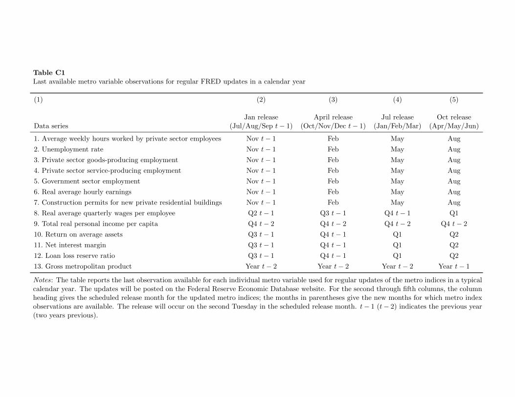
Table C1Last available metro variable observations for regular FRED updates in a calendar year

(1) (2) (3) (4) (5)

Jan release April release Jul release Oct releaseData series (Jul/Aug/Sep t� 1) (Oct/Nov/Dec t� 1) (Jan/Feb/Mar) (Apr/May/Jun)

1. Average weekly hours worked by private sector employees Nov t� 1 Feb May Aug

2. Unemployment rate Nov t� 1 Feb May Aug

3. Private sector goods-producing employment Nov t� 1 Feb May Aug

4. Private sector service-producing employment Nov t� 1 Feb May Aug

5. Government sector employment Nov t� 1 Feb May Aug

6. Real average hourly earnings Nov t� 1 Feb May Aug

7. Construction permits for new private residential buildings Nov t� 1 Feb May Aug

8. Real average quarterly wages per employee Q2 t� 1 Q3 t� 1 Q4 t� 1 Q1

9. Total real personal income per capita Q4 t� 2 Q4 t� 2 Q4 t� 2 Q4 t� 2

10. Return on average assets Q3 t� 1 Q4 t� 1 Q1 Q2

11. Net interest margin Q3 t� 1 Q4 t� 1 Q1 Q2

12. Loan loss reserve ratio Q3 t� 1 Q4 t� 1 Q1 Q2

13. Gross metropolitan product Year t� 2 Year t� 2 Year t� 2 Year t� 1

Notes: The table reports the last observation available for each individual metro variable used for regular updates of the metro indices in a typicalcalendar year. The updates will be posted on the Federal Reserve Economic Database website. For the second through fifth columns, the columnheading gives the scheduled release month for the updated metro indices; the months in parentheses give the new months for which metro indexobservations are available. The release will occur on the second Tuesday in the scheduled release month. t� 1 (t� 2) indicates the previous year(two years previous).