methods to estimate railway capacity and … to estimate...methods to estimate railway capacity and...
TRANSCRIPT
General rights Copyright and moral rights for the publications made accessible in the public portal are retained by the authors and/or other copyright owners and it is a condition of accessing publications that users recognise and abide by the legal requirements associated with these rights.
Users may download and print one copy of any publication from the public portal for the purpose of private study or research.
You may not further distribute the material or use it for any profit-making activity or commercial gain
You may freely distribute the URL identifying the publication in the public portal If you believe that this document breaches copyright please contact us providing details, and we will remove access to the work immediately and investigate your claim.
Downloaded from orbit.dtu.dk on: Feb 23, 2020
Methods to estimate railway capacity and passenger delays
Landex, Alex
Publication date:2008
Document VersionPublisher's PDF, also known as Version of record
Link back to DTU Orbit
Citation (APA):Landex, A. (2008). Methods to estimate railway capacity and passenger delays. Kgs. Lyngby, Denmark:Technical University of Denmark.
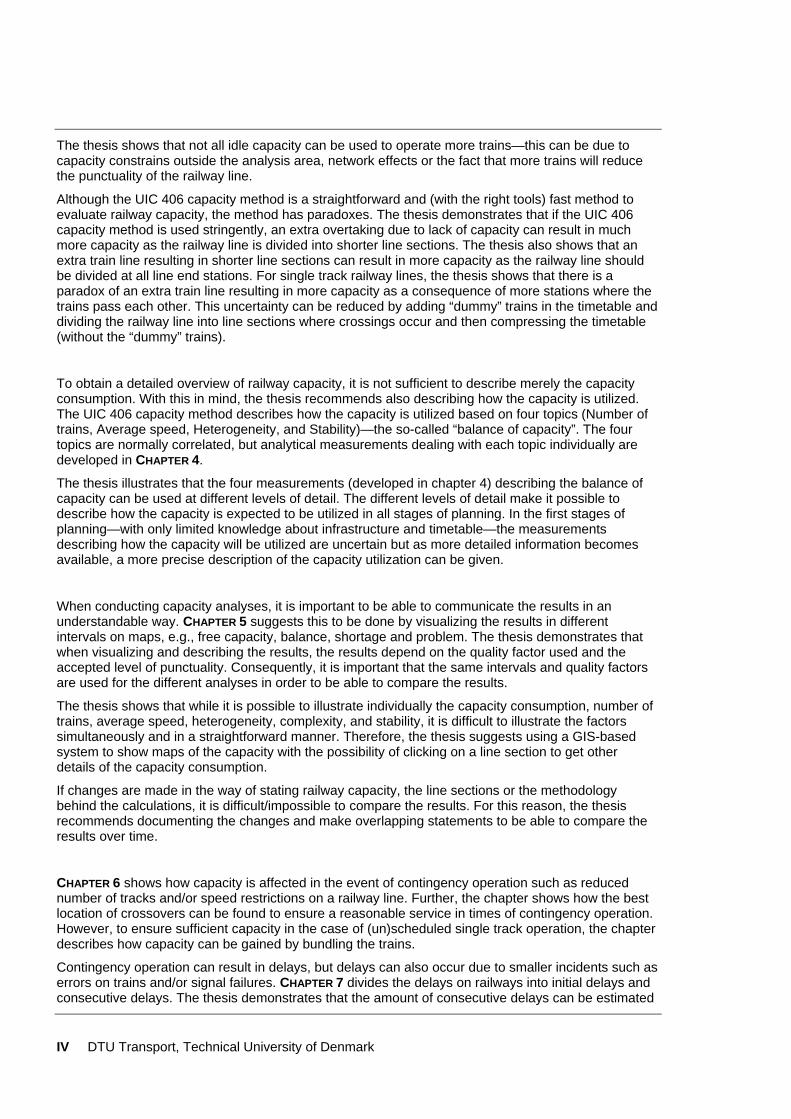
95,4%
84,0%
90,6%
80,5%
95,4%90,3% 91,4%
86,8%92,7%
85,0%
60%
70%
80%
90%
100%
Infrastructure
E l ti
15,7% 17,3%22,5% 22,5%
19,6%
0%
10%
20%
30%
40%
50%
Morning Day Afternoon Other time Total
Train regularity [%] Passenger regularity [%] Arrivals before time [%]
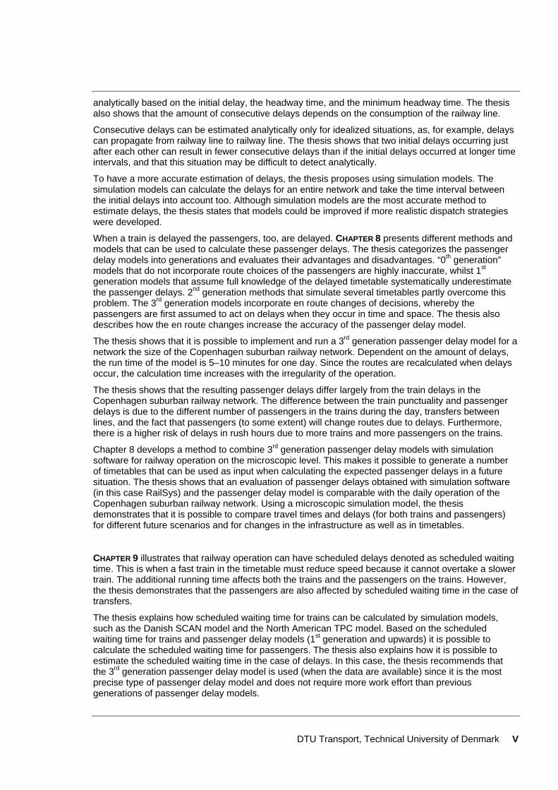
Timetable
Evaluation
Si l ti
Passengerdelaymodel
Simulation UIC 406 capacityanalysis
Methods to estimate railway capacity and passenger delaysAlex LandexPhD thesisPhD thesisNovember 2008

Methods to estimate railway capacity and passenger delays
PhD thesis
Alex Landex Technical University of Denmark
Department of Transport
Supervisor: Professor Otto Anker Nielsen
Technical University of Denmark Department of Transport
Co-supervisor: External lecturer Anders H. Kaas
Atkins Danmark A/S &
Technical University of Denmark Department of Transport
November 2008


DTU Transport, Technical University of Denmark I
Preface This PhD thesis is the result of research work at the Department of Transport at the Technical University of Denmark. I started working in this department in 2003 when I worked on research projects and taught courses in Rail Traffic Engineering, Public Transport Planning and ArcGIS and Traffic Planning. One year later, I started this project on “Methods to estimate railway capacity and passenger delays”. The work was conducted on a ¾ time basis to allow me to continue teaching the courses in Rail Traffic Engineering and Public Transport Planning.
Writing this thesis has been a lot of hard work, but it has also been a lot of fun, for most of the time. Railways are not only the topic of my thesis but have also been, and still are, a hot topic in the media: underinvestment in the railway network, reduced speed on the main railway lines, new IC4 trains not put into service and, above all, delays. When studying railway systems and, in my case, “Methods to estimate railway capacity and passenger delays”, there is always something to talk about at parties!
Despite the fact that a PhD thesis does not get finished during social chats, there is no chance of finishing the job without other people. In fact, the summary below is just an attempt to cover the people and organizations whose inputs have been truly indispensable for completing my dissertation.
First of all, I would like to thank my co-supervisor Anders H. Kaas, without his introductory course on railway systems I would never have started writing this thesis. Anders is also thanked for being there when I needed motivation, new ideas or a good academic and/or scientific discussion during the work on this thesis—also before he became co-supervisor. Professor Otto Anker Nielsen is also thanked for supervising the project.
Bernd Schittenhelm was always ready for a good discussion about my work, and I enjoyed his provocative contributions and practical views on the subject. His proofreading of articles and the thesis has contributed to improving the output, and he has also given me many useful ideas for further research. I am happy that Bernd has now decided to become a PhD student himself, and I am looking forward to many new, rewarding discussions.
My thanks to Rapidis Ltd, who coded the passenger delay model presented in this thesis. Also thanks to Rasmus Dyhr Frederiksen, Bjarke Brun and Philip Bagger from Rapidis Ltd and Stephen Hansen from DTU Transport (now Rapidis Ltd), who assisted in making the (different versions of) the 3rd generation passenger delay model work together with RailSys.
The project has given rise to a series of articles and academic discussions. I thank all involved, both the people and the organizations. In particular, I want to thank Rail Net Denmark (Banedanmark), the National Rail Authority (Trafikstyrelsen), the Danish State Railways (DSB), and my co-authors on the articles.
Also, thanks to all the students on the course Rail Traffic Engineering and all the other persons who (deliberately or unwittingly) asked “tricky” questions about my work. This has been a source of inspiration and also a reminder to explain the sometimes tricky answers in a straightforward way.
Things did not always go as planned. And it was in those cases that I was especially thankful to my good colleagues, my friends and my family for their tremendous support. Sten Hansen gave me excellent guidance and advice. He also had a knack of pointing me in the right direction to find the best solutions to get the project moving.
Finally, thanks to all those other persons who assisted and supported me over the last four years. And a heartfelt thank you to the Technical Information Centre of Denmark (DTIC) for the invaluable help provided the last months of this project. Without this help, it would not have been possible to finalize this thesis.
Alex Landex Kgs. Lyngby, November 2008

II DTU Transport, Technical University of Denmark
DTU Transport, Technical University of Denmark III
Summary CHAPTER 1 explains the importance of having knowledge about railway capacity and how, over time, it has become possible to operate more trains by improving the infrastructure and rolling stock. Additionally, the aim and structure of the thesis are outlined.
CHAPTER 2 describes the difficulties of defining railway capacity, which depends on the infrastructure, the rolling stock and the actual timetable. In 2004, the International Union of Railways (UIC) published a leaflet giving a method to measure the capacity consumption of line sections based on the actual infrastructure and timetable (and thereby also the rolling stock used)—the UIC 406 capacity method.
The UIC 406 capacity method can be used in an analytical way determining the capacity consumption as the sum of the occupation time, buffer time, and time supplements. This sum is then divided by the time window observed. In addition to the analytical way of determining the capacity consumption, capacity consumption can be measured by compressing the timetable graphs as much as possible for the line section and then using the compression ratio as a measurement of the capacity consumption.
CHAPTER 3 shows how the UIC 406 method can be expounded in different ways. It is, therefore, important to divide the railway line into line sections of the “right” length. The thesis illustrates that it may be reasonable not to divide the railway lines into line sections at all locations as suggested in the UIC 406 capacity method. Not dividing the railway lines into line sections at overtakings may result in additional challenges when working out the capacity consumption. To handle overtakings in line sections, the thesis recommends maintaining the order of the trains (both before and after the overtaking) and allowing for changing the dwell time to the minimum dwelling time for exchange of passengers and/or the needed time for start moving (a freight train) after a complete halt.
At crossing stations, line end stations, larger stations with shunting, and junctions, the thesis recommends that attention be paid to conflicting train paths. The crossing station’s lack of ability to handle parallel movement can reduce the capacity of the line section as the dwell time is extended. The line end stations can be limiting for the capacity because not all avoiding lines may be scheduled and/or the layover time is longer than needed. The thesis recommends dealing with this by reducing the layover time to a minimum and by using all possible avoiding tracks. Larger stations with shunting can be difficult to examine due to lack of knowledge of the exact shunting operation. Therefore, the thesis recommends that larger stations should be evaluated according to the published timetable and only the known shunting operations but with a higher quality factor or other time supplements to include the remaining shunting implicitly. At junctions and crossing stations, conflicting train routes can result in reduced capacity for some train paths. Accordingly, the thesis recommends extending the analysis area for crossing stations and junctions to include the entire crossing station and/or junction.
For line sections with more than two tracks, the thesis illustrates that attention must be paid to the order of the trains at both the beginning and the end of the line section as otherwise there is a risk of additional overtakings occurring. Furthermore, more tracks can result in uneven capacity consumption. Accordingly, the thesis recommends allowing trains to change from one track to another if there is a large difference in the capacity consumption of the tracks.
If tracks are located apart from each other it might be difficult to determine how many tracks a railway line comprises. Therefore, the thesis proposes that the railway line is considered as one line section if there is mainly one-way operation on the tracks and if both corridors are served in both directions and different stations are serviced it should be considered as two lines.
The thesis puts forward a method to use the UIC 406 capacity leaflet to evaluate the future capacity consumption without knowing the exact infrastructure and/or timetable. This is done by using successive calculation, where the capacity consumption is calculated for the best-case situation (where the lowest capacity consumption is achieved by bundling the trains) and the worst-case situation (where the highest capacity consumption is achieved) together with the capacity consumption of a proposed future timetable. These capacity consumptions are then weighted together to describe the expected capacity consumption.
IV DTU Transport, Technical University of Denmark
The thesis shows that not all idle capacity can be used to operate more trains—this can be due to capacity constrains outside the analysis area, network effects or the fact that more trains will reduce the punctuality of the railway line.
Although the UIC 406 capacity method is a straightforward and (with the right tools) fast method to evaluate railway capacity, the method has paradoxes. The thesis demonstrates that if the UIC 406 capacity method is used stringently, an extra overtaking due to lack of capacity can result in much more capacity as the railway line is divided into shorter line sections. The thesis also shows that an extra train line resulting in shorter line sections can result in more capacity as the railway line should be divided at all line end stations. For single track railway lines, the thesis shows that there is a paradox of an extra train line resulting in more capacity as a consequence of more stations where the trains pass each other. This uncertainty can be reduced by adding “dummy” trains in the timetable and dividing the railway line into line sections where crossings occur and then compressing the timetable (without the “dummy” trains).
To obtain a detailed overview of railway capacity, it is not sufficient to describe merely the capacity consumption. With this in mind, the thesis recommends also describing how the capacity is utilized. The UIC 406 capacity method describes how the capacity is utilized based on four topics (Number of trains, Average speed, Heterogeneity, and Stability)—the so-called “balance of capacity”. The four topics are normally correlated, but analytical measurements dealing with each topic individually are developed in CHAPTER 4.
The thesis illustrates that the four measurements (developed in chapter 4) describing the balance of capacity can be used at different levels of detail. The different levels of detail make it possible to describe how the capacity is expected to be utilized in all stages of planning. In the first stages of planning—with only limited knowledge about infrastructure and timetable—the measurements describing how the capacity will be utilized are uncertain but as more detailed information becomes available, a more precise description of the capacity utilization can be given.
When conducting capacity analyses, it is important to be able to communicate the results in an understandable way. CHAPTER 5 suggests this to be done by visualizing the results in different intervals on maps, e.g., free capacity, balance, shortage and problem. The thesis demonstrates that when visualizing and describing the results, the results depend on the quality factor used and the accepted level of punctuality. Consequently, it is important that the same intervals and quality factors are used for the different analyses in order to be able to compare the results.
The thesis shows that while it is possible to illustrate individually the capacity consumption, number of trains, average speed, heterogeneity, complexity, and stability, it is difficult to illustrate the factors simultaneously and in a straightforward manner. Therefore, the thesis suggests using a GIS-based system to show maps of the capacity with the possibility of clicking on a line section to get other details of the capacity consumption.
If changes are made in the way of stating railway capacity, the line sections or the methodology behind the calculations, it is difficult/impossible to compare the results. For this reason, the thesis recommends documenting the changes and make overlapping statements to be able to compare the results over time.
CHAPTER 6 shows how capacity is affected in the event of contingency operation such as reduced number of tracks and/or speed restrictions on a railway line. Further, the chapter shows how the best location of crossovers can be found to ensure a reasonable service in times of contingency operation. However, to ensure sufficient capacity in the case of (un)scheduled single track operation, the chapter describes how capacity can be gained by bundling the trains.
Contingency operation can result in delays, but delays can also occur due to smaller incidents such as errors on trains and/or signal failures. CHAPTER 7 divides the delays on railways into initial delays and consecutive delays. The thesis demonstrates that the amount of consecutive delays can be estimated
DTU Transport, Technical University of Denmark V
analytically based on the initial delay, the headway time, and the minimum headway time. The thesis also shows that the amount of consecutive delays depends on the consumption of the railway line.
Consecutive delays can be estimated analytically only for idealized situations, as, for example, delays can propagate from railway line to railway line. The thesis shows that two initial delays occurring just after each other can result in fewer consecutive delays than if the initial delays occurred at longer time intervals, and that this situation may be difficult to detect analytically.
To have a more accurate estimation of delays, the thesis proposes using simulation models. The simulation models can calculate the delays for an entire network and take the time interval between the initial delays into account too. Although simulation models are the most accurate method to estimate delays, the thesis states that models could be improved if more realistic dispatch strategies were developed.
When a train is delayed the passengers, too, are delayed. CHAPTER 8 presents different methods and models that can be used to calculate these passenger delays. The thesis categorizes the passenger delay models into generations and evaluates their advantages and disadvantages. “0th generation” models that do not incorporate route choices of the passengers are highly inaccurate, whilst 1st generation models that assume full knowledge of the delayed timetable systematically underestimate the passenger delays. 2nd generation methods that simulate several timetables partly overcome this problem. The 3rd generation models incorporate en route changes of decisions, whereby the passengers are first assumed to act on delays when they occur in time and space. The thesis also describes how the en route changes increase the accuracy of the passenger delay model.
The thesis shows that it is possible to implement and run a 3rd generation passenger delay model for a network the size of the Copenhagen suburban railway network. Dependent on the amount of delays, the run time of the model is 5–10 minutes for one day. Since the routes are recalculated when delays occur, the calculation time increases with the irregularity of the operation.
The thesis shows that the resulting passenger delays differ largely from the train delays in the Copenhagen suburban railway network. The difference between the train punctuality and passenger delays is due to the different number of passengers in the trains during the day, transfers between lines, and the fact that passengers (to some extent) will change routes due to delays. Furthermore, there is a higher risk of delays in rush hours due to more trains and more passengers on the trains.
Chapter 8 develops a method to combine 3rd generation passenger delay models with simulation software for railway operation on the microscopic level. This makes it possible to generate a number of timetables that can be used as input when calculating the expected passenger delays in a future situation. The thesis shows that an evaluation of passenger delays obtained with simulation software (in this case RailSys) and the passenger delay model is comparable with the daily operation of the Copenhagen suburban railway network. Using a microscopic simulation model, the thesis demonstrates that it is possible to compare travel times and delays (for both trains and passengers) for different future scenarios and for changes in the infrastructure as well as in timetables.
CHAPTER 9 illustrates that railway operation can have scheduled delays denoted as scheduled waiting time. This is when a fast train in the timetable must reduce speed because it cannot overtake a slower train. The additional running time affects both the trains and the passengers on the trains. However, the thesis demonstrates that the passengers are also affected by scheduled waiting time in the case of transfers.
The thesis explains how scheduled waiting time for trains can be calculated by simulation models, such as the Danish SCAN model and the North American TPC model. Based on the scheduled waiting time for trains and passenger delay models (1st generation and upwards) it is possible to calculate the scheduled waiting time for passengers. The thesis also explains how it is possible to estimate the scheduled waiting time in the case of delays. In this case, the thesis recommends that the 3rd generation passenger delay model is used (when the data are available) since it is the most precise type of passenger delay model and does not require more work effort than previous generations of passenger delay models.
VI DTU Transport, Technical University of Denmark
Calculating scheduled waiting times for candidate timetables makes it possible to test different timetable strategies and choose the best strategy for the final timetable. This can improve the timetables for both the operator(s) and the passengers. In the longer term, the approach can be used at the centralized control offices in the event of contingency operation. Here, an evaluation of the network effects can be used to select the dispatching strategy that results in the smallest possible amount of additional travel time.
The differences between the different kinds of delay (train delays, passenger delays and scheduled waiting time) are illustrated through simple, but representative, case examples in CHAPTER 10. The examples demonstrate that 3rd generation passenger delay models are more realistic than previous generations of passenger delay models, and that train delays can result in a situation where it is beneficial to passengers as the passengers as a whole spend less time in the railway system.
The chapter also shows that passenger delay models can be used to evaluate and test various timetable alternatives, passenger delays in the case of contingency operation, and dispatching strategies. The simple cases presented in the thesis can be calculated either manually or by a passenger delay model. However, in more complicated cases (e.g. larger networks or situations where different case examples are combined) the calculations become too complicated to work out manually, and a passenger delay model becomes necessary.
CHAPTER 11 illustrates that railway operation is affected by network effects because a change in one part of the network can influence other parts of the network too. The chapter shows that the influence can be far from where the original change was made. This is because the train services are (often) relatively long and because most railway systems have a high degree of interdependency, as trains cannot cross/overtake each other everywhere in the network.
The thesis shows that network effects depend on the given infrastructure and timetable and can result in longer travel times for trains and passengers. Furthermore, the thesis shows that the network effects can result in reduced capacity as some trains or train services can make it impossible to operate other planned/desired trains or train services. Therefore, the thesis recommends including network effects in the analyses.
The chapter divides network effects into four categories: network effects in the schedule planning phase, network effects for trains, network effects for passengers, and network effects in the case of contingency operation. The thesis shows that the network effects can affect both trains and passengers, resulting in a “planned delay”. Therefore, the thesis recommends using scheduled waiting time to quantify the network effects in the following way:
• Network effects in the timetabling process—scheduled waiting time for both trains and passengers. In the screening phase it is recommended to calculate the scheduled waiting time for trains only, while it can be calculated for both trains and passengers in the later phases
• Network effects for trains—scheduled waiting time for trains
• Network effects for passengers—scheduled waiting time for passengers
• Network effects for contingency operation—scheduled waiting time for trains if the analysis is conducted from a purely operational viewpoint, but scheduled waiting time for both trains and passengers is preferred in general plans for contingency operation. The scheduled waiting time can be calculated based on either the optimal timetable or the planned timetable
The thesis states that the amount of network effects in the railway network increases with the complexity of the operation, which is why there are more network effects in cases with planned transfers. Therefore, the thesis recommends that timetable planners should be more precise when timetabling for larger networks (and networks with transfers) than for a railway line with no track connection to other railway lines.

DTU Transport, Technical University of Denmark VII
Main contributions of the thesis The thesis is a methodological contribution to extending the applicability of the UIC 406 capacity method and the calculation of delays in railway operation. The thesis uses a systems engineering approach to examine the UIC 406 methodology in a methodical way and to work out a consistent way of expounding the said methodology. The thesis also presents applicable models to calculate delays for both trains and passengers. These different delay models are examined and compared.
Throughout the thesis, focus is on applicability of the methods. Therefore, both fictitious and representative examples and illustrative cases from the real world are used to illustrate the approaches. The main contributions of this thesis are:
• Thorough examination of the UIC 406 capacity method
• Recommendations of how to expound the UIC 406 methodology in a coherent way
• Analytical method to describe how railway capacity is utilized
• Methodology to state railway capacity according to the UIC 406 method
• Methods to describe and present railway capacity
• Evaluation of approaches to calculate passenger delays
• Estimation of future passenger delays
• Comparison of train delays and passenger delays
• Methodology to estimate scheduled waiting time for trains and passengers
• Quantification of network effects using scheduled waiting time
• Applicability of the UIC 406 capacity methodology and the delay models

VIII DTU Transport, Technical University of Denmark
DTU Transport, Technical University of Denmark IX
Index PREFACE .................................................................................................................................................................... I SUMMARY .............................................................................................................................................................. III Main contributions of the thesis ..................................................................................................................... VII INDEX .................................................................................................................................................................... IX CHAPTER 1 1 INTRODUCTION ...................................................................................................................................................... 1 1.1 Aim of the thesis .......................................................................................................................................... 2 1.2 The structure of the thesis ............................................................................................................................ 4 CHAPTER 2 2 RAILWAY CAPACITY .............................................................................................................................................. 7 2.1 Definition of railway capacity ...................................................................................................................... 8 2.2 The UIC 406 capacity method ................................................................................................................... 12 2.3 Practical use of the UIC 406 capacity method ........................................................................................... 14 2.4 Summary .................................................................................................................................................... 15 CHAPTER 3 3 MEASURING RAILWAY CAPACITY ........................................................................................................................ 17 3.1 Difference of double and single track railway lines according to UIC 406 ............................................... 18 3.2 Dividing Railway lines into line sections ................................................................................................... 18 3.2.1 Line end stations on open line ........................................................................................................... 23 3.3 Crossing stations ........................................................................................................................................ 24 3.3.1 Crossing while in motion ................................................................................................................... 26 3.3.2 Partly double track ............................................................................................................................. 27 3.4 Junctions ..................................................................................................................................................... 27 3.5 Overtaking .................................................................................................................................................. 29 3.6 Line end stations ........................................................................................................................................ 30 3.7 Large stations and shunting ........................................................................................................................ 31 3.8 Changing between tracks at stations and at lines with more than two tracks ............................................. 32 3.9 When is it a single track line versus a double track line? ........................................................................... 38 3.10 The possibility of using idle capacity to operate more trains ................................................................... 40 3.11 Use of UIC 406 without exact infrastructure and/or timetable ................................................................. 44 3.12 Paradoxes of the UIC 406 capacity method ............................................................................................. 46 3.12.1 Overtakings ...................................................................................................................................... 46 3.12.2 Extra trains ....................................................................................................................................... 46 3.13 Using the UIC 406 capacity method in practice ....................................................................................... 49 3.14 Workflow of capacity analysis ................................................................................................................. 50 3.15 Recommendations on measuring railway capacity .................................................................................. 52 3.14 Summary .................................................................................................................................................. 54 CHAPTER 4 4 UTILIZATION OF RAILWAY CAPACITY .................................................................................................................. 57 4.1 Number of trains ........................................................................................................................................ 57 4.2 Heterogeneity ............................................................................................................................................. 58 4.3 Average speed ............................................................................................................................................ 61 4.4 Stability ...................................................................................................................................................... 64 4.4.1 Complexity of stations based on track layout .................................................................................... 65 4.4.2 Complexity of stations using probabilities ........................................................................................ 66 4.4.3 Complexity of operation at stations using minimum headway times ................................................ 67 4.4.4 From complexity to stability .............................................................................................................. 68 4.5 Discussion .................................................................................................................................................. 69 4.6 Summary .................................................................................................................................................... 70
X DTU Transport, Technical University of Denmark
CHAPTER 5 5 CAPACITY STATEMENT ........................................................................................................................................ 71 5.1 Intervals of capacity statements ................................................................................................................. 72 5.2 Quality factor ............................................................................................................................................. 74 5.3 Capacity utilization .................................................................................................................................... 75 5.4 Variation in railway capacity ..................................................................................................................... 78 5.5 Example of capacity statement .................................................................................................................. 78 5.6 Development in railway capacity .............................................................................................................. 80 5.7 From capacity of railway lines to railway networks .................................................................................. 80 5.8 Summary .................................................................................................................................................... 81 CHAPTER 6 6 CAPACITY IN CASE OF CONTINGENCY OPERATION ............................................................................................... 83 6.1 Unscheduled single track operation ........................................................................................................... 83 6.1.1 Need for crossovers ........................................................................................................................... 83 6.1.2 Bundled operation ............................................................................................................................. 85 6.1.3 Change of timetables ......................................................................................................................... 86 6.2 Reduced speed ........................................................................................................................................... 87 6.3 Summary .................................................................................................................................................... 88 CHAPTER 7 7 TRAIN DELAYS .................................................................................................................................................... 89 7.1 Delays ........................................................................................................................................................ 90 7.2 High capacity consumption – higher risk of (consecutive) delays ............................................................. 91 7.3 Delay propagation on double track lines with homogeneous traffic .......................................................... 92 7.4 Delays in case of heterogeneous and/or single track operation ................................................................. 96 7.4.1 Same speed and stop pattern but variation in headway times on double track lines ......................... 97 7.4.2 Heterogeneous operation on double track lines ................................................................................ 97 7.4.3 Single track ....................................................................................................................................... 99 7.5 Delays found by simulation ..................................................................................................................... 101 7.6 Summary .................................................................................................................................................. 105 CHAPTER 8 8 PASSENGER DELAYS .......................................................................................................................................... 107 8.1 Literature review ...................................................................................................................................... 108 8.2 Methods to calculate passenger delays .................................................................................................... 110 8.2.1 Traditional calculation – 0th generation ........................................................................................... 110 8.2.2 Optimal route choice – 1st generation .............................................................................................. 113 8.2.3 1½ generation .................................................................................................................................. 114 8.2.4 2nd generation .................................................................................................................................. 114 8.2.5 3rd generation ................................................................................................................................... 114 8.2.6 Comparison between models .......................................................................................................... 116 8.3 The 3rd generation model in practice ....................................................................................................... 116 8.4 Results on empirical data in the Copenhagen suburban rail network ...................................................... 117 8.5 Calculation of future passenger delays by simulation ............................................................................. 119 8.6 Possibilities with the passenger delay model ........................................................................................... 122 8.7 How to improve the 3rd generation passenger delay model ..................................................................... 123 8.8 Summary .................................................................................................................................................. 124 CHAPTER 9 9 SCHEDULED WAITING TIME ............................................................................................................................... 125 9.1 Scheduled waiting time for trains ............................................................................................................ 125 9.2 Scheduled waiting time for passengers .................................................................................................... 127 9.3 Calculation of scheduled waiting time for trains ..................................................................................... 128 9.4 Calculation of scheduled waiting time for passengers ............................................................................. 130 9.5 Discussion ................................................................................................................................................ 132 9.6 Summary .................................................................................................................................................. 132
DTU Transport, Technical University of Denmark XI
CHAPTER 10 10 COMPARISON OF DELAYS ON RAILWAYS .......................................................................................................... 135 10.1 Case 1: High frequent operation with a homogeneous stop pattern ....................................................... 135 10.2 Case 2: Lost transfer ............................................................................................................................... 136 10.3 Case 3: Optimistic versus 3rd generation passenger delay models ......................................................... 137 10.3.1 Delay at Stop D—difference between passenger delay models ..................................................... 138 10.3.2 Importance of threshold value ....................................................................................................... 138 10.4 Case 4: Heterogeneous operation ........................................................................................................... 139 10.4.1 The local train waits for the intercity to pass ................................................................................. 140 10.4.2 The local train departs on time and is not overtaken ..................................................................... 141 10.4.3 Comparing the dispatching strategies ............................................................................................ 142 10.5 Case 5: Scheduled waiting time ............................................................................................................. 142 10.5.1 No scheduled waiting time ............................................................................................................ 143 10.5.2 Scheduled waiting time as additional running time ....................................................................... 144 10.5.3 Scheduled waiting time as an additional stop ................................................................................ 144 10.5.4 Homogenized operation ................................................................................................................. 145 10.5.5 Comparing the strategies for scheduled waiting time .................................................................... 146 10.6 Summary ................................................................................................................................................ 146 CHAPTER 11 11 NETWORK EFFECTS .......................................................................................................................................... 147 11.1 Network effects in general ..................................................................................................................... 148 11.2 Network effects in the train schedule planning process ......................................................................... 150 11.3 Network effects for trains and passengers .............................................................................................. 152 11.4 Network effects for contingency operation ............................................................................................ 152 11.5 Quantifying network effects ................................................................................................................... 153 11.6 Discussion .............................................................................................................................................. 155 11.7 Summary ................................................................................................................................................ 156 CHAPTER 12 12 CONCLUSION ................................................................................................................................................... 159 12.1 Main contributions of the thesis ............................................................................................................. 160 12.2 Recommendations for future research .................................................................................................... 161 REFERENCES ......................................................................................................................................................... 163 LIST OF FIGURES ................................................................................................................................................... 173 LIST OF TABLES .................................................................................................................................................... 179 APPENDIXES 1 DEFINITIONS ...................................................................................................................................................... 183 2 SYMBOLS ........................................................................................................................................................... 187 3 STATION ABBREVIATIONS .................................................................................................................................. 189 4 DIVISION OF THE DANISH RAILWAY NETWORK INTO LINE SECTIONS ................................................................. 191 5 DIVIDING THE SUBURBAN RAILWAY NETWORK INTO LINE SECTIONS ................................................................. 193 6 MAPS OF THE DANISH RAILWAY NETWORK ....................................................................................................... 199

XII DTU Transport, Technical University of Denmark

DTU Transport, Technical University of Denmark 1
Chapter 1
1 Introduction In the early days of railways, railway capacity was more or less a question of whether or not there were railway tracks. However, as the railway system grew and more trains were operated, lack of capacity was experienced. These capacity problems were (partly) solved by doubling railway tracks and extending the railway stations—and in some cases by building completely new railway lines and/or stations. Construction work solved many of the capacity problems, but technological development (e.g. signalling technology) also played a role.
How capacity problems in the railway system have been “solved” over the years can be illustrated by an example from Copenhagen. In 1847 Copenhagen got its first railway line—the railway line to Roskilde. The following years saw Copenhagen with more railway lines and to gather all the railway lines in one station, a new central station was built in 1864.
As the traffic increased and more railway lines were opened the central station from 1864 experienced lack of capacity. This was remedied by extending the station, several times. In 1911 a new central station was opened, but it was not until several years later when a tunnel through Copenhagen was built that all trains stopped at this new station.
In 1921 all four tracks through central Copenhagen were in use. Nevertheless, new capacity problems on the two suburban tracks arose already in the 1920s (Poulsen 1997). These capacity problems were solved by upgrading and electrifying the railway line and gradually switching to electrical (S-train) operation from 1934 to 19681. Capacity problems still occurred, but more capacity could be gained (and more trains could be operated) by the change to modern interlocking systems (HKT) in 19722. This “new” interlocking system has since been optimized to be able to handle more trains per hour. The development in the number of trains can be seen in figure 1.1.
0
5
10
15
20
25
30
1920 1930 1940 1950 1960 1970 1980 1990 2000 2010Year
Num
ber
of tr
ains
per
dir
ectio
n pe
r ho
ur
S-trainsOther trainsTotal
Figure 1.1: Number of trains on the suburban tracks in central Copenhagen in the peak hours3.
1 The S-trains had better acceleration and needed less time at the platforms. 2 HKT – HastighedsKontrol og Togstop (speed control and train stop)—is the ATP system of the suburban railway lines in Copenhagen, albeit, not all railway lines are equipped with HKT or similar. 3 Data derived from timetables from 1921 to 2008. Data include only the two suburban tracks and not the metro and the trains on the tracks of the long distance trains.
2 DTU Transport, Technical University of Denmark
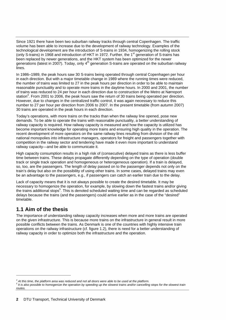
Since 1921 there have been two suburban railway tracks through central Copenhagen. The traffic volume has been able to increase due to the development of railway technology. Examples of the technological development are the introduction of S-trains in 1934, homogenizing the rolling stock (only S-trains) in 1968 and introduction of HKT in 1972. Further, the 1st generation of S-trains has been replaced by newer generations, and the HKT system has been optimized for the newer generations (latest in 2007). Today, only 4th generation S-trains are operated on the suburban railway lines.
In 1986–1989, the peak hours saw 30 S-trains being operated through central Copenhagen per hour in each direction. But with a major timetable change in 1989 where the running times were reduced, the number of trains was limited to 27 in the peak hours per direction in order to be able to maintain reasonable punctuality and to operate more trains in the daytime hours. In 2000 and 2001, the number of trains was reduced to 24 per hour in each direction due to construction of the Metro at Nørreport station4. From 2001 to 2006, the peak hours saw the return of 30 trains being operated per direction. However, due to changes in the centralized traffic control, it was again necessary to reduce this number to 27 per hour per direction from 2006 to 2007. In the present timetable (from autumn 2007) 30 trains are operated in the peak hours in each direction.
Today’s operations, with more trains on the tracks than when the railway line opened, pose new demands. To be able to operate the trains with reasonable punctuality, a better understanding of railway capacity is required. How railway capacity is measured and how the capacity is utilized has become important knowledge for operating more trains and ensuring high quality in the operation. The recent development of more operators on the same railway lines resulting from division of the old national monopolies into infrastructure managers, operators for freight and passengers together with competition in the railway sector and tendering have made it even more important to understand railway capacity—and be able to communicate it.
High capacity consumption results in a high risk of (consecutive) delayed trains as there is less buffer time between trains. These delays propagate differently depending on the type of operation (double track or single track operation and homogeneous or heterogeneous operation). If a train is delayed, so, too, are the passengers. The length of delay passed on to the passenger depends not only on the train’s delay but also on the possibility of using other trains. In some cases, delayed trains may even be an advantage to the passengers, e.g., if passengers can catch an earlier train due to the delay.
Lack of capacity means that it is not always possible to create the desired timetable. It may be necessary to homogenize the operation, for example, by slowing down the fastest trains and/or giving the trains additional stops5. This is denoted scheduled waiting time and can be regarded as scheduled delays because the trains (and the passengers) could arrive earlier as in the case of the “desired” timetable.
1.1 Aim of the thesis The importance of understanding railway capacity increases when more and more trains are operated on the given infrastructure. This is because more trains on the infrastructure in general result in more possible conflicts between the trains. As Denmark is one of the countries with highly intensive train operations on the railway infrastructure (cf. figure 1.2), there is need for a better understanding of railway capacity in order to optimize both the infrastructure and the operation.
4 At this time, the platform area was reduced and not all doors were able to be used at the platform. 5 It is also possible to homogenize the operation by speeding up the slowest trains and/or cancelling stops for the slowest train routes.

DTU Transport, Technical University of Denmark 3
0 5 10 15 20 25 30 35 40 451,000 train km per km railway
Finland
Sweden
Norway
Poland
France
Italy
Germany
Spain
Luxemburg
Belgium
United Kingdom
Denmark
Netherlands
Switzerland
Figure 1.2: Utilization of railway networks. Data from (National Rail Authority 2007b)6.
Denmark has a more homogeneous operation of the railway network than other countries (e.g. Germany and France), which allows the high capacity utilization. The homogeneous operation can be explained by the fact that there is no high-speed operation and only a limited amount of freight transport. Despite Denmark being one of the counties that operates the most trains on the railway infrastructure, few plans exist to build more tracks. This means that the current trend, where more trains are operated on the existing infrastructure (cf. figure 1.3), seems set to continue. Accordingly, there is a need for a better understanding of railway capacity to optimize the infrastructure and operation. In this way it will be possible to ensure the same level of service regarding delays on the railway network—or even improve it.
192021222324252627282930313233
1,00
0 tra
in k
m p
er k
m ra
ilway
per
yea
r x
Figure 1.3: Development in utilization of the Danish railway infrastructure. Data from (Statistics Denmark 2007a, Statistics Denmark 2007b).
6 The data on Denmark from (National Rail Authority 2007b) was incorrect. Therefore, the value for Denmark has been corrected based on information from J. Brix from the National Rail Authority.
4 DTU Transport, Technical University of Denmark
On this background, this thesis examines railway capacity in a methodical way from a systems engineering approach. For this, we used the widely accepted UIC 406 capacity method from 2004 (UIC 2004), which is commonly used in Denmark (and other countries). The examination of railway capacity will result in a better understanding of capacity and in suggestions and recommendations about how the UIC 406 methodology should be expounded. Based on the examination of railway capacity, delays for both trains and passengers on the railway network are examined as a method to evaluate the railway operation—the past, present and future operation. Throughout the thesis the focus is on the applicability of the methodologies presented. Therefore, the thesis presents both fictitious, but typical, examples and illustrative examples from the real world.
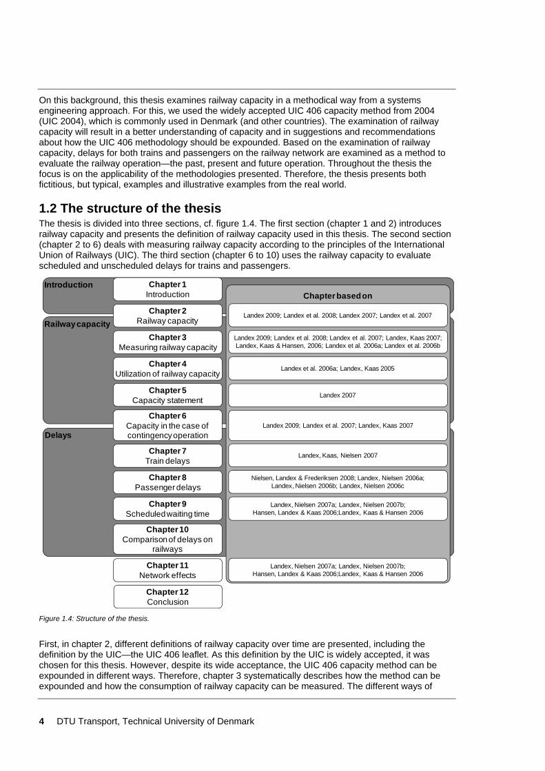
1.2 The structure of the thesis The thesis is divided into three sections, cf. figure 1.4. The first section (chapter 1 and 2) introduces railway capacity and presents the definition of railway capacity used in this thesis. The second section (chapter 2 to 6) deals with measuring railway capacity according to the principles of the International Union of Railways (UIC). The third section (chapter 6 to 10) uses the railway capacity to evaluate scheduled and unscheduled delays for trains and passengers.
Chapter based on
Railway capacity
Introduction
Delays
Chapter 4Utilization of railway capacity
Chapter 3Measuring railway capacity
Chapter 6Capacity in the case ofcontingency operation
Chapter 5Capacity statement
Chapter 1Introduction
Chapter 2Railway capacity
Chapter 9Scheduled waiting time
Chapter 7Train delays
Chapter 8Passenger delays
Chapter 10Comparison of delays on
railways
Chapter 11Network effects
Chapter 12Conclusion
Landex 2007
Landex et al. 2006a; Landex, Kaas 2005
Nielsen, Landex & Frederiksen 2008; Landex, Nielsen 2006a;Landex, Nielsen 2006b; Landex, Nielsen 2006c
Landex, Nielsen 2007a; Landex, Nielsen 2007b;Hansen, Landex & Kaas 2006;Landex, Kaas & Hansen 2006
Landex, Nielsen 2007a; Landex, Nielsen 2007b;Hansen, Landex & Kaas 2006;Landex, Kaas & Hansen 2006
Landex 2009; Landex et al. 2008; Landex et al. 2007; Landex, Kaas 2007;Landex, Kaas & Hansen, 2006; Landex et al. 2006a; Landex et al. 2006b
Landex 2009; Landex et al. 2007; Landex, Kaas 2007
Landex, Kaas, Nielsen 2007
Landex 2009; Landex et al. 2008; Landex 2007; Landex et al. 2007
Figure 1.4: Structure of the thesis.
First, in chapter 2, different definitions of railway capacity over time are presented, including the definition by the UIC—the UIC 406 leaflet. As this definition by the UIC is widely accepted, it was chosen for this thesis. However, despite its wide acceptance, the UIC 406 capacity method can be expounded in different ways. Therefore, chapter 3 systematically describes how the method can be expounded and how the consumption of railway capacity can be measured. The different ways of
DTU Transport, Technical University of Denmark 5
expounding the UIC 406 method are tested on both real-world infrastructure and timetables and on fictitious examples inspired by real-world cases. Based on this examination of the UIC 406, the thesis suggests how the method should be expounded. These suggestions have since become the basis of the Danish method of how to conduct capacity analyses using the UIC 406 capacity method.
The consumption of railway capacity does not only depend on how many trains are operated it also depends on how the capacity is utilized. For example, a heterogeneous operation, where fast trains catch up with slower trains, results in higher capacity consumption than a homogeneous operation where all trains are operated with the same speed. Chapter 4 presents and suggests methods of how to measure the capacity utilization according to the UIC 406 (number of trains, average speed, heterogeneity and stability). The suggested methods are tested on fictitious examples and real-world cases.
Based on the findings in chapter 2 to 4, chapter 5 describes how railway capacity can be stated. However, not all railway operation is carried out as planned in the public timetable. Sometimes, breakdowns of the infrastructure or trains occur in addition to the infrastructure having to be maintained and renewed. In these cases, less capacity is available, and contingency operation is necessary. Chapter 6 describes how the capacity is affected in cases of possessions and contingency operation.
When delays happen they may propagate to other trains. This delay propagation depends on the capacity consumption, the homogeneity of the operation, and whether it is single track operation or whether more tracks are available. The delay propagation can be estimated either mathematically or by simulation. Chapter 7 describes the train delays and tests the delay propagation on a fictitious case example.
When trains become delayed the passengers in the trains become delayed too. Therefore, chapter 8 describes different methods to calculate passenger delays. This includes the development from simple methods considering only the number of passengers boarding and alighting the trains to the most advanced (3rd generation) passenger delay models taking into account passengers’ different route choice possibilities. The chapter tests a 3rd generation passenger delay model on the Copenhagen suburban railway network.
Not all delays are unplanned. Some delays are scheduled in the timetable as scheduled waiting times. These scheduled waiting times are incorporated in the timetable because faster trains catch up slower trains due to lack of capacity. Chapter 9 describes these scheduled waiting times and how they can be measured.
Chapter 10 illustrates the different types of delays through small case examples inspired by real-world operation. The chapter also compares the different types of delays to illustrate the differences between train delays and passenger delays. Towards the end of the thesis, chapter 11 describes the importance of the network effects of the railway network when examining both railway capacity and delays. The importance of the network effects is illustrated by fictitious examples as well as a large-scale infrastructure project. Lastly, chapter 12 present a conclusion.
In the appendices, Appendix 1 gives an explanation of the terms and definitions used in this thesis. Appendices 2 and 3 give a summary list of the notation and the station abbreviations used in the thesis. Appendix 4 lists how the Danish railway network has been divided into line sections according to the UIC 406 capacity method, and Appendix 5 explains the considerations behind dividing the Copenhagen suburban railway network into line sections. Lastly, Appendix 6 shows maps of the Danish railway network.

6 DTU Transport, Technical University of Denmark
DTU Transport, Technical University of Denmark 7
Chapter 2
2 Railway capacity It is relatively straightforward to determine the capacity on roads: it is normally determined merely as vehicles per hour. Capacity on railways is, however, more difficult to determine because the capacity depends on the infrastructure, the timetable and the rolling stock (Kaas 1998b).
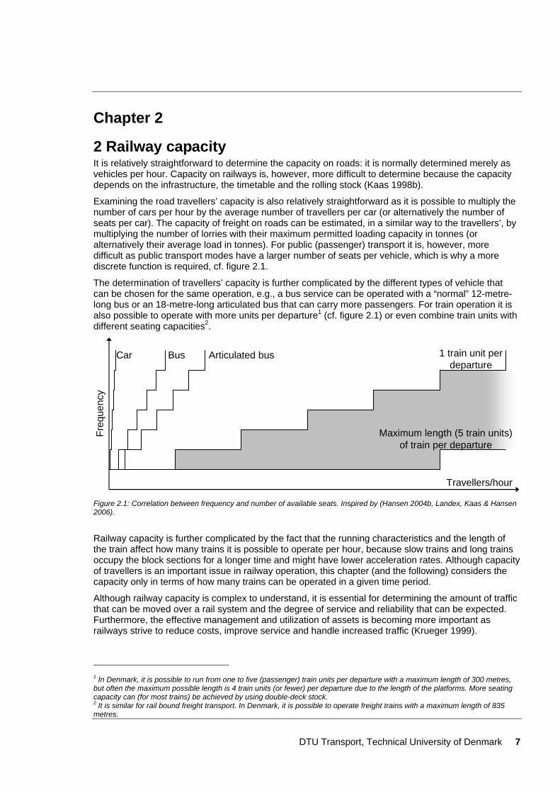
Examining the road travellers’ capacity is also relatively straightforward as it is possible to multiply the number of cars per hour by the average number of travellers per car (or alternatively the number of seats per car). The capacity of freight on roads can be estimated, in a similar way to the travellers’, by multiplying the number of lorries with their maximum permitted loading capacity in tonnes (or alternatively their average load in tonnes). For public (passenger) transport it is, however, more difficult as public transport modes have a larger number of seats per vehicle, which is why a more discrete function is required, cf. figure 2.1.
The determination of travellers’ capacity is further complicated by the different types of vehicle that can be chosen for the same operation, e.g., a bus service can be operated with a “normal” 12-metre-long bus or an 18-metre-long articulated bus that can carry more passengers. For train operation it is also possible to operate with more units per departure1 (cf. figure 2.1) or even combine train units with different seating capacities2.
Car
Freq
uenc
y
Bus Articulated bus 1 train unit perdeparture
Maximum length (5 train units)of train per departure
Travellers/hour
Figure 2.1: Correlation between frequency and number of available seats. Inspired by (Hansen 2004b, Landex, Kaas & Hansen 2006).
Railway capacity is further complicated by the fact that the running characteristics and the length of the train affect how many trains it is possible to operate per hour, because slow trains and long trains occupy the block sections for a longer time and might have lower acceleration rates. Although capacity of travellers is an important issue in railway operation, this chapter (and the following) considers the capacity only in terms of how many trains can be operated in a given time period.
Although railway capacity is complex to understand, it is essential for determining the amount of traffic that can be moved over a rail system and the degree of service and reliability that can be expected. Furthermore, the effective management and utilization of assets is becoming more important as railways strive to reduce costs, improve service and handle increased traffic (Krueger 1999).
1 In Denmark, it is possible to run from one to five (passenger) train units per departure with a maximum length of 300 metres, but often the maximum possible length is 4 train units (or fewer) per departure due to the length of the platforms. More seating capacity can (for most trains) be achieved by using double-deck stock. 2 It is similar for rail bound freight transport. In Denmark, it is possible to operate freight trains with a maximum length of 835 metres.
8 DTU Transport, Technical University of Denmark
This chapter is the background for the following chapters about railway capacity (chapters 3 to 6). Therefore, this chapter presents different definitions of railway capacity in section 2.1. Section 2.2 presents a definition and method developed by the International Union of Railways (UIC) to measure the consumption of railway capacity. This method developed by the UIC is the method used in this thesis. Section 2.3 then gives a brief overview of how the UIC method to measure the capacity consumption works before section 2.4 summarizes the chapter.
2.1 Definition of railway capacity Railway capacity is a complex, loosely defined term that has numerous meanings (Krueger 1999), and the definitions differ by country (Rothengatter 1996). In 2004 the International Union of Railways (UIC) (re)defined railway capacity as (UIC 2004):
Capacity as such does not exist. Railway infrastructure capacity depends on the way it is utilized.
This definition of railway capacity is followed by a guideline for how railway capacity can be measured given the actual infrastructure and the actual timetable.
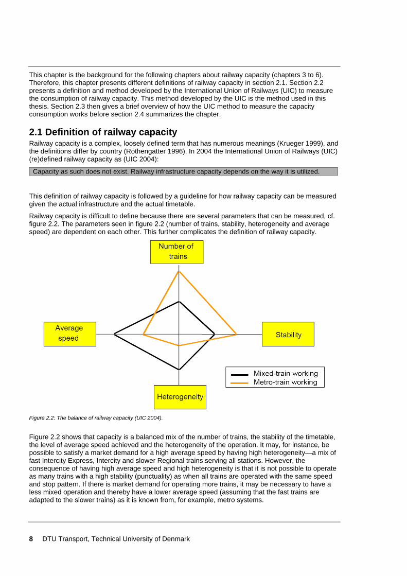
Railway capacity is difficult to define because there are several parameters that can be measured, cf. figure 2.2. The parameters seen in figure 2.2 (number of trains, stability, heterogeneity and average speed) are dependent on each other. This further complicates the definition of railway capacity.
Figure 2.2: The balance of railway capacity (UIC 2004).
Figure 2.2 shows that capacity is a balanced mix of the number of trains, the stability of the timetable, the level of average speed achieved and the heterogeneity of the operation. It may, for instance, be possible to satisfy a market demand for a high average speed by having high heterogeneity—a mix of fast Intercity Express, Intercity and slower Regional trains serving all stations. However, the consequence of having high average speed and high heterogeneity is that it is not possible to operate as many trains with a high stability (punctuality) as when all trains are operated with the same speed and stop pattern. If there is market demand for operating more trains, it may be necessary to have a less mixed operation and thereby have a lower average speed (assuming that the fast trains are adapted to the slower trains) as it is known from, for example, metro systems.
DTU Transport, Technical University of Denmark 9
It could be argued that the description of railway capacity presented by the UIC includes only the timetable and not the infrastructure, the rolling stock or the quality of service. However, both the rolling stock and the infrastructure are implicitly included because they are important parameters for the timetable, while the quality is described by the stability (punctuality), the number of trains (frequency), the average speed (travel speed) and the heterogeneity (the mix of trains).
Due to the interaction between the infrastructure and the timetable, and that the capacity depends on the timetable, it is difficult—or even impossible—to define railway capacity in a consistent way. Therefore, railway capacity has been defined differently over time, e.g.:
• Railway capacity is the ability of the carrier to supply as required the necessary services within acceptable service levels and costs so as to meet the present and projected demand for such services3 (Kahan 1979)
• The capacity of a railway line is the ability to operate trains with an acceptable punctuality (Skartsæterhagen 1993)
• The theoretical capacity is defined to be the maximal number of trains that can be operated on a railway link (Rothengatter 1996)
• The capacity of an infrastructure facility is the ability to operate the trains with an acceptable punctuality (Kaas 1998b)
• Capacity is a measure of the ability to move a specific amount of traffic over a defined rail line with a given set of resources under a specific service plan (Krueger 1999)
• The only true measure of capacity therefore is the range of timetables that the network could support, tested against future demand scenarios and expected operational performance (Wood, Robertson 2002)
• Capacity can be defined as the capability of the infrastructure to handle one or several timetables (Hansen 2004b)
• Capacity is defined as the maximum number of trains which can pass a given point on a railway line in a given time interval (Longo, Stok 2007)
• Capacity may be defined as the ratio between the chosen time window and the sum of average minimum headway time and required average buffer time (Oetting 2007)
• The capacity of the infrastructure is room on the track that can be used to operate trains (Jernbaneverket 2007)
• The number of trains that can be incorporated into a timetable that is conflict-free, commercially attractive, compliant with regulatory requirements, and can be operated in the face of anticipated levels of primary delay whilst meeting agreed performance targets (Barter 2008)4
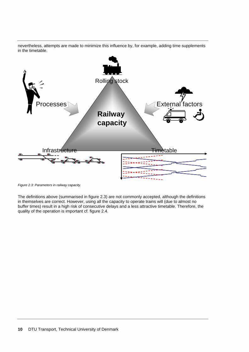
The above definitions of railway capacity show (although many definitions are alike) that there is great variation in how railway capacity can be defined. A reason for this variety is that most definitions of railway capacity are defined nationally or in connection with a specific project. Common to the definitions is that the railway capacity depends on the railway infrastructure and the timetable—and, thereby, implicitly on the rolling stock used, cf. figure 2.3.
Railway capacity depends not “only” on the rolling stock, the infrastructure and the timetable—sometimes the capacity is reduced due to processes in the operation such as time consuming departure procedures or external factors such as the weather and problems with the rolling stock. Processes can be procedures at departures, staff schedules, many passengers at the stations etc., while the external factors can be, e.g., weather conditions, breakdowns and accidents. Common to the processes and external factors is that it is not possible to predict their influence on the operation;
3 (Kahan 1979) has eight different definitions of practical capacity for railway lines. 4 (Barter 2008) quotes (Nock 1980)
10 DTU Transport, Technical University of Denmark
nevertheless, attempts are made to minimize this influence by, for example, adding time supplements in the timetable.
Rolling stock
TimetableInfrastructure
Railwaycapacity
Processes External factors
Figure 2.3: Parameters in railway capacity.
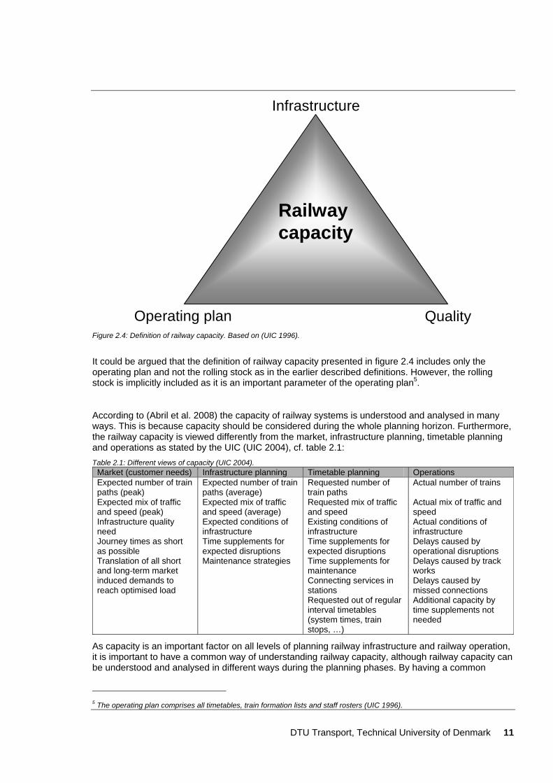
The definitions above (summarised in figure 2.3) are not commonly accepted, although the definitions in themselves are correct. However, using all the capacity to operate trains will (due to almost no buffer times) result in a high risk of consecutive delays and a less attractive timetable. Therefore, the quality of the operation is important cf. figure 2.4.
DTU Transport, Technical University of Denmark 11
Infrastructure
QualityOperating plan
Railwaycapacity
Figure 2.4: Definition of railway capacity. Based on (UIC 1996).
It could be argued that the definition of railway capacity presented in figure 2.4 includes only the operating plan and not the rolling stock as in the earlier described definitions. However, the rolling stock is implicitly included as it is an important parameter of the operating plan5.
According to (Abril et al. 2008) the capacity of railway systems is understood and analysed in many ways. This is because capacity should be considered during the whole planning horizon. Furthermore, the railway capacity is viewed differently from the market, infrastructure planning, timetable planning and operations as stated by the UIC (UIC 2004), cf. table 2.1: Table 2.1: Different views of capacity (UIC 2004).
Market (customer needs) Infrastructure planning Timetable planning Operations Expected number of train paths (peak) Expected mix of traffic and speed (peak) Infrastructure quality need Journey times as short as possible Translation of all short and long-term market induced demands to reach optimised load
Expected number of train paths (average) Expected mix of traffic and speed (average) Expected conditions of infrastructure Time supplements for expected disruptions Maintenance strategies
Requested number of train paths Requested mix of traffic and speed Existing conditions of infrastructure Time supplements for expected disruptions Time supplements for maintenance Connecting services in stations Requested out of regular interval timetables (system times, train stops, …)
Actual number of trains Actual mix of traffic and speed Actual conditions of infrastructure Delays caused by operational disruptions Delays caused by track works Delays caused by missed connections Additional capacity by time supplements not needed
As capacity is an important factor on all levels of planning railway infrastructure and railway operation, it is important to have a common way of understanding railway capacity, although railway capacity can be understood and analysed in different ways during the planning phases. By having a common
5 The operating plan comprises all timetables, train formation lists and staff rosters (UIC 1996).
12 DTU Transport, Technical University of Denmark
definition of railway capacity it is easier to communicate capacity between organisations and planning phases.
By choosing one definition of railway capacity, it is also important to note that only one way of stating capacity is chosen. The description of capacity by the International Union of Railways (UIC) in the UIC 406 capacity leaflet also describes how capacity should be measured. This way of understanding railway capacity is straightforward and has become widely accepted. Therefore, no new definition of railway capacity is introduced in this thesis: the UIC capacity description (and methodology) is used.
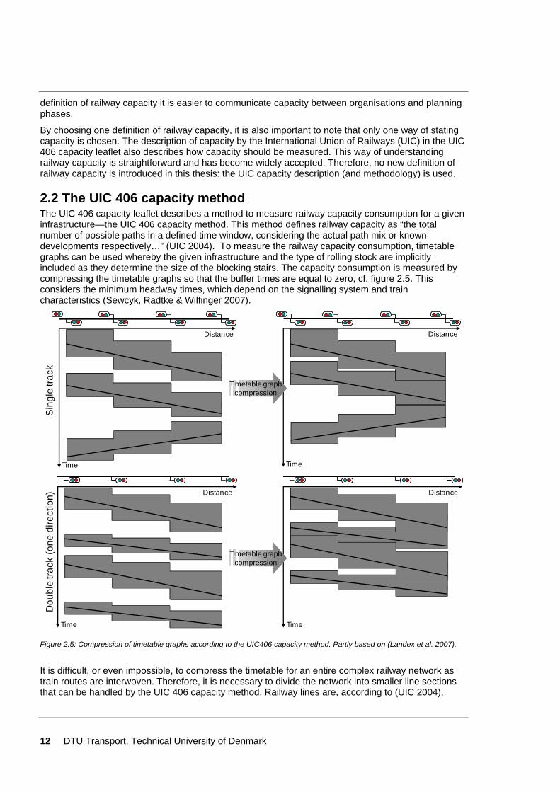
2.2 The UIC 406 capacity method The UIC 406 capacity leaflet describes a method to measure railway capacity consumption for a given infrastructure—the UIC 406 capacity method. This method defines railway capacity as “the total number of possible paths in a defined time window, considering the actual path mix or known developments respectively…” (UIC 2004). To measure the railway capacity consumption, timetable graphs can be used whereby the given infrastructure and the type of rolling stock are implicitly included as they determine the size of the blocking stairs. The capacity consumption is measured by compressing the timetable graphs so that the buffer times are equal to zero, cf. figure 2.5. This considers the minimum headway times, which depend on the signalling system and train characteristics (Sewcyk, Radtke & Wilfinger 2007).
Sin
gle
track
Dou
ble
track
(one
dire
ctio
n)
Time
Distance
Timetable graphcompression
Distance
Time
Distance
Time
Distance
Time
Timetable graphcompression
Figure 2.5: Compression of timetable graphs according to the UIC406 capacity method. Partly based on (Landex et al. 2007).
It is difficult, or even impossible, to compress the timetable for an entire complex railway network as train routes are interwoven. Therefore, it is necessary to divide the network into smaller line sections that can be handled by the UIC 406 capacity method. Railway lines are, according to (UIC 2004),
DTU Transport, Technical University of Denmark 13
divided into smaller line sections at junctions, overtaking stations, line end stations, transitions between double track and single track (or any other number of tracks) and at crossing stations.
In practice, the UIC 406 capacity method can be used manually for any given line section by using a timetabling system that has conflict detection, e.g., RailSys (Siefer, Radtke 2005) and the TPS system6 (Kaas, Goossmann 2004) used in Denmark. Some timetabling systems (e.g. RailSys and Viriato) have built-in functionalities that can assist the user in calculating the capacity consumption according to the UIC 406 capacity method (Abril et al. 2008, Barber et al. 2007, RMCon 2007).
The total capacity consumption (k) can also be calculated in a more analytical way by summing the infrastructure occupation time (tA), the buffer time (tB), the time supplement for single track lines (tC) and maintenance (tD) (UIC 2004):
Formula 2.1: k = tA + tB + tC + tD
The capacity consumption in per cent (K) can be worked out based on the total capacity consumption measured in time (k) and the chosen time window (tU) (UIC 2004):
Formula 2.2: K = k * 100%/tU
The expressions in formula 2.1 and formula 2.2 can be expressed differently to calculate the capacity consumption in one step (Landex et al. 2007).
Formula 2.3: K = (tA + tB + tC + tD) * 100%/tU
The infrastructure occupation time (tA) and the time window (tU) are the most important factors in formula 2.3. This is because the infrastructure occupation time makes up most of the capacity consumption of the time window examined (tU). The buffer time (tB) is normally (in the Danish context) set equal to zero but can be set to a different value to improve the quality of the operation by ensuring fewer consecutive delays. It could be argued that the buffer time is a kind of quality factor—see section 5.3.
The time supplement for single track operation (tC) can be added at the crossing stations the same way to improve the quality of the operation by reducing the risk of consecutive delays. Alternatively, the time supplement for single track operation can be used in the completely analytically examination of the capacity consumption. This is done by considering the running time from the entrance of the station to the release of the train route before the train in the opposite direction can depart from the platform together with the extra time it might take if the crossing station cannot handle parallel movements. In the Danish context, the time supplement for single track operation is normally set to zero.
The time supplement for maintenance (tD) can be used in cases of possession planning for maintenance and/or construction works. In Denmark, these supplements are not included in the UIC 406 capacity analysis.
The railway capacity consumption can be optimized, or minimized, by changing the parameters. Reducing the buffer time (or quality factor) will lead to less capacity consumption. However, it should be noted that the buffer time (together with time supplements) improves the stability of the timetable (Longo, Stok 2007). Additionally, the time supplements for single track operation and maintenance are time supplements that improve the stability of the timetable.
If the stability of the timetable is not to be reduced, only the infrastructure occupation time can be reduced. This can be done by bundling the trains so that trains with the same stopping pattern and
6 Previously, the TPS system was called STRAX.
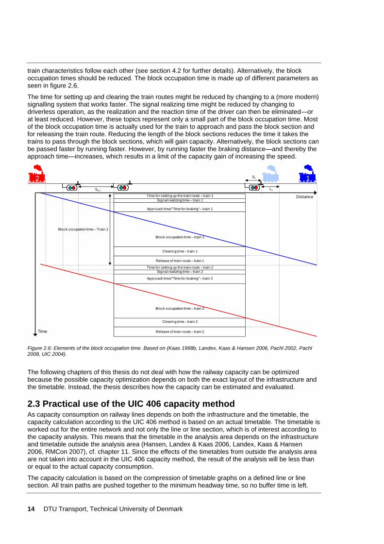
14 DTU Transport, Technical University of Denmark
train characteristics follow each other (see section 4.2 for further details). Alternatively, the block occupation times should be reduced. The block occupation time is made up of different parameters as seen in figure 2.6.
The time for setting up and clearing the train routes might be reduced by changing to a (more modern) signalling system that works faster. The signal realizing time might be reduced by changing to driverless operation, as the realization and the reaction time of the driver can then be eliminated—or at least reduced. However, these topics represent only a small part of the block occupation time. Most of the block occupation time is actually used for the train to approach and pass the block section and for releasing the train route. Reducing the length of the block sections reduces the time it takes the trains to pass through the block sections, which will gain capacity. Alternatively, the block sections can be passed faster by running faster. However, by running faster the braking distance—and thereby the approach time—increases, which results in a limit of the capacity gain of increasing the speed.
2 1
Time for setting up the train route – train 1
Time for setting up the train route – train 2
Signal realizing time – train 1
Approach time/”Time for braking” – train 1
Block occupation time – train 1
Clearing time – train 1
Release of train route – train 1
Signal realizing time – train 2
Approach time/”Time for braking” – train 2
Block occupation time – train 2
Clearing time – train 2
Release of train route – train 2
Sb,2 L1
Ss
Block occupation time – Train 1
Time
Distance
Figure 2.6: Elements of the block occupation time. Based on (Kaas 1998b, Landex, Kaas & Hansen 2006, Pachl 2002, Pachl 2008, UIC 2004).
The following chapters of this thesis do not deal with how the railway capacity can be optimized because the possible capacity optimization depends on both the exact layout of the infrastructure and the timetable. Instead, the thesis describes how the capacity can be estimated and evaluated.
2.3 Practical use of the UIC 406 capacity method As capacity consumption on railway lines depends on both the infrastructure and the timetable, the capacity calculation according to the UIC 406 method is based on an actual timetable. The timetable is worked out for the entire network and not only the line or line section, which is of interest according to the capacity analysis. This means that the timetable in the analysis area depends on the infrastructure and timetable outside the analysis area (Hansen, Landex & Kaas 2006, Landex, Kaas & Hansen 2006, RMCon 2007), cf. chapter 11. Since the effects of the timetables from outside the analysis area are not taken into account in the UIC 406 capacity method, the result of the analysis will be less than or equal to the actual capacity consumption.
The capacity calculation is based on the compression of timetable graphs on a defined line or line section. All train paths are pushed together to the minimum headway time, so no buffer time is left.
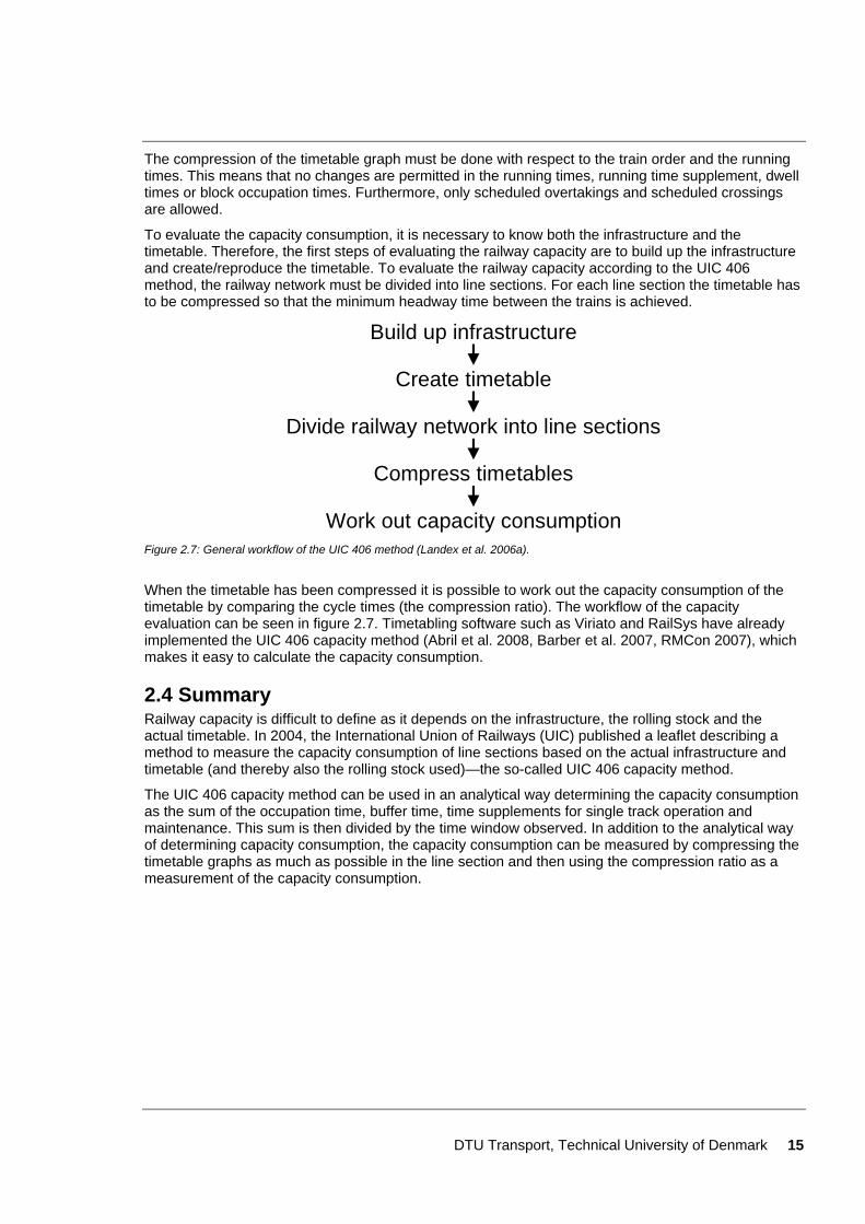
DTU Transport, Technical University of Denmark 15
The compression of the timetable graph must be done with respect to the train order and the running times. This means that no changes are permitted in the running times, running time supplement, dwell times or block occupation times. Furthermore, only scheduled overtakings and scheduled crossings are allowed.
To evaluate the capacity consumption, it is necessary to know both the infrastructure and the timetable. Therefore, the first steps of evaluating the railway capacity are to build up the infrastructure and create/reproduce the timetable. To evaluate the railway capacity according to the UIC 406 method, the railway network must be divided into line sections. For each line section the timetable has to be compressed so that the minimum headway time between the trains is achieved.
Create timetable
Divide railway network into line sections
Compress timetables
Work out capacity consumption
Build up infrastructure
Figure 2.7: General workflow of the UIC 406 method (Landex et al. 2006a).
When the timetable has been compressed it is possible to work out the capacity consumption of the timetable by comparing the cycle times (the compression ratio). The workflow of the capacity evaluation can be seen in figure 2.7. Timetabling software such as Viriato and RailSys have already implemented the UIC 406 capacity method (Abril et al. 2008, Barber et al. 2007, RMCon 2007), which makes it easy to calculate the capacity consumption.
2.4 Summary Railway capacity is difficult to define as it depends on the infrastructure, the rolling stock and the actual timetable. In 2004, the International Union of Railways (UIC) published a leaflet describing a method to measure the capacity consumption of line sections based on the actual infrastructure and timetable (and thereby also the rolling stock used)—the so-called UIC 406 capacity method.
The UIC 406 capacity method can be used in an analytical way determining the capacity consumption as the sum of the occupation time, buffer time, time supplements for single track operation and maintenance. This sum is then divided by the time window observed. In addition to the analytical way of determining capacity consumption, the capacity consumption can be measured by compressing the timetable graphs as much as possible in the line section and then using the compression ratio as a measurement of the capacity consumption.

16 DTU Transport, Technical University of Denmark
DTU Transport, Technical University of Denmark 17
Chapter 3
3 Measuring railway capacity The previous chapter gave an overview of how the capacity consumption of railway lines can be worked out by the UIC 406 capacity method published by the International Union of Railways (UIC) in 2004. Many organisations have adopted the UIC 406 capacity method as it (with the right tools) is a straightforward, fast and effective way to measure the capacity consumption of railway lines. In the past years, this method has been applied in several studies (e.g., (Landex et al. 2006b, Atkins Danmark A/S 2005, Wahlborg 2004)).
The UIC 406 capacity method can be expounded in different ways, which is also stated by the UIC1 (UIC 2004). Furthermore, while the UIC 406 capacity method acts as a reference, it does not function as a law or a norm, even though the leaflets coexist with the national and international laws (UIC). Despite the different ways of expounding the UIC 406 method potentially leading to different results, few analyses of the differences exist.
As the UIC 406 capacity method is open to interpretation, this chapter describes the analyses that have been done. Together with some adaptations and interpretations made on the UIC 406 capacity method, these analyses have become the basis of how to use the method in Denmark. The chapter is organized as follows:
• Section 3.1: Differences between double and single track railway lines
• Section 3.2: How to divide railway lines into line sections
• Section 3.3: Handling of crossing stations
• Section 3.4: Handling of junctions
• Section 3.5: Handling of overtaking stations
• Section 3.6: Handling of line end stations
• Section 3.7: Handling of large stations with shunting operation
• Section 3.8: Changing between tracks at stations and railway lines with multiple tracks
• Section 3.9: When a railway line is single track versus double track
• Section 3.10: The possibility of using idle capacity to operate more trains
• Section 3.11: Use of UIC 406 without exact infrastructure and/or timetable
• Section 3.12: Paradoxes of the UIC 406 capacity method
• Section 3.13: Using the UIC 406 capacity method in practice
• Section 3.14: Recommendations on the workflow for the UIC 406 capacity method
• Section 3.15: Recommendations on measuring railway capacity
• Section 3.16: Summary
This chapter describes how the capacity consumption of railway lines can be estimated but not how the railway capacity is utilized—this is described in the next chapter (chapter 4) followed by a chapter describing how railway capacity can be stated (chapter 5). This is followed by a description of how the railway capacity is affected by contingency operation (chapter 6).
1For example, in (UIC 2004) it is stated “The total number of possible paths in a defined time window, considering the actual path mix or known developments respectively and the IM’s own assumptions”.
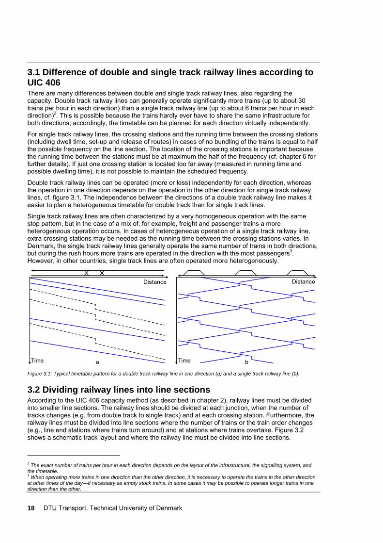
18 DTU Transport, Technical University of Denmark
3.1 Difference of double and single track railway lines according to UIC 406 There are many differences between double and single track railway lines, also regarding the capacity. Double track railway lines can generally operate significantly more trains (up to about 30 trains per hour in each direction) than a single track railway line (up to about 6 trains per hour in each direction)2. This is possible because the trains hardly ever have to share the same infrastructure for both directions; accordingly, the timetable can be planned for each direction virtually independently.
For single track railway lines, the crossing stations and the running time between the crossing stations (including dwell time, set-up and release of routes) in cases of no bundling of the trains is equal to half the possible frequency on the line section. The location of the crossing stations is important because the running time between the stations must be at maximum the half of the frequency (cf. chapter 6 for further details). If just one crossing station is located too far away (measured in running time and possible dwelling time), it is not possible to maintain the scheduled frequency.
Double track railway lines can be operated (more or less) independently for each direction, whereas the operation in one direction depends on the operation in the other direction for single track railway lines, cf. figure 3.1. The independence between the directions of a double track railway line makes it easier to plan a heterogeneous timetable for double track than for single track lines.
Single track railway lines are often characterized by a very homogeneous operation with the same stop pattern, but in the case of a mix of, for example, freight and passenger trains a more heterogeneous operation occurs. In cases of heterogeneous operation of a single track railway line, extra crossing stations may be needed as the running time between the crossing stations varies. In Denmark, the single track railway lines generally operate the same number of trains in both directions, but during the rush hours more trains are operated in the direction with the most passengers3. However, in other countries, single track lines are often operated more heterogeneously.
a b
Distance Distance
Time Time Figure 3.1: Typical timetable pattern for a double track railway line in one direction (a) and a single track railway line (b).
3.2 Dividing railway lines into line sections According to the UIC 406 capacity method (as described in chapter 2), railway lines must be divided into smaller line sections. The railway lines should be divided at each junction, when the number of tracks changes (e.g. from double track to single track) and at each crossing station. Furthermore, the railway lines must be divided into line sections where the number of trains or the train order changes (e.g., line end stations where trains turn around) and at stations where trains overtake. Figure 3.2 shows a schematic track layout and where the railway line must be divided into line sections.
2 The exact number of trains per hour in each direction depends on the layout of the infrastructure, the signalling system, and the timetable. 3 When operating more trains in one direction than the other direction, it is necessary to operate the trains in the other direction at other times of the day—if necessary as empty stock trains. In some cases it may be possible to operate longer trains in one direction than the other.
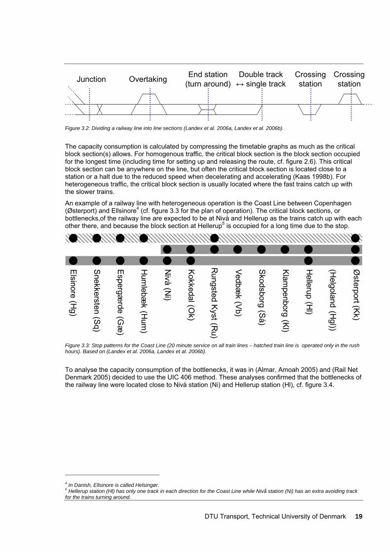
DTU Transport, Technical University of Denmark 19
Overtaking End station(turn around)Junction Double track
↔ single trackCrossingstation
Crossingstation
Figure 3.2: Dividing a railway line into line sections (Landex et al. 2006a, Landex et al. 2006b).
The capacity consumption is calculated by compressing the timetable graphs as much as the critical block section(s) allows. For homogenous traffic, the critical block section is the block section occupied for the longest time (including time for setting up and releasing the route, cf. figure 2.6). This critical block section can be anywhere on the line, but often the critical block section is located close to a station or a halt due to the reduced speed when decelerating and accelerating (Kaas 1998b). For heterogeneous traffic, the critical block section is usually located where the fast trains catch up with the slower trains.
An example of a railway line with heterogeneous operation is the Coast Line between Copenhagen (Østerport) and Ellsinore4 (cf. figure 3.3 for the plan of operation). The critical block sections, or bottlenecks,of the railway line are expected to be at Nivå and Hellerup as the trains catch up with each other there, and because the block section at Hellerup5 is occupied for a long time due to the stop.
Elsinore (Hg)
Snekkersten (S
q)
Espergæ
rde (Gæ
)
Hum
lebæk (H
um)
Nivå (N
i)
Kokkedal (Ok)
Rungsted K
yst (Ru)
Vedbæk (V
b)
Skodsborg (Så)
Klampenborg (Kl)
Hellerup (H
l)
(Helgoland (H
gl))
Østerport (K
k)
Figure 3.3: Stop patterns for the Coast Line (20 minute service on all train lines – hatched train line is operated only in the rush hours). Based on (Landex et al. 2006a, Landex et al. 2006b).
To analyse the capacity consumption of the bottlenecks, it was in (Almar, Amoah 2005) and (Rail Net Denmark 2005) decided to use the UIC 406 method. These analyses confirmed that the bottlenecks of the railway line were located close to Nivå station (Ni) and Hellerup station (Hl), cf. figure 3.4.
4 In Danish, Ellsinore is called Helsingør. 5 Hellerup station (Hl) has only one track in each direction for the Coast Line while Nivå station (Ni) has an extra avoiding track for the trains turning around.
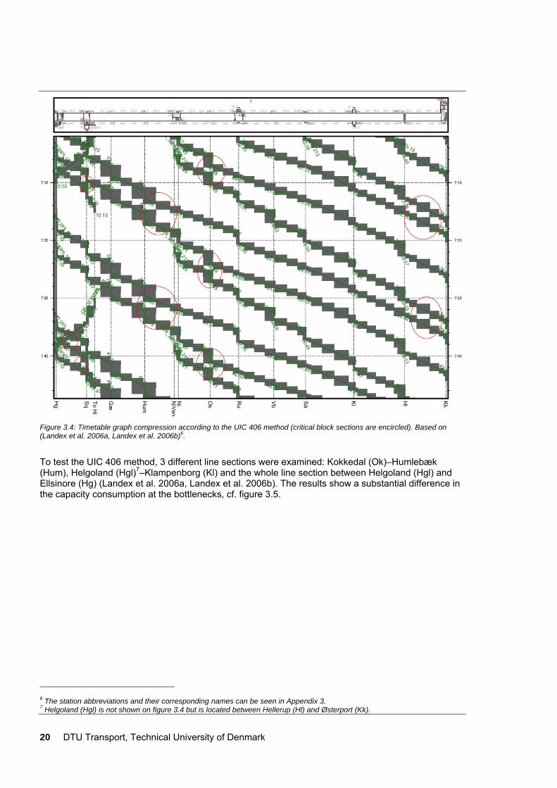
20 DTU Transport, Technical University of Denmark
Hg
Hl
Sq Så Kl KkTo Hi
Gæ
Hum
NiV
enN
i
Ok
Ru
Vb
Figure 3.4: Timetable graph compression according to the UIC 406 method (critical block sections are encircled). Based on (Landex et al. 2006a, Landex et al. 2006b)6.
To test the UIC 406 method, 3 different line sections were examined: Kokkedal (Ok)–Humlebæk (Hum), Helgoland (Hgl)7–Klampenborg (Kl) and the whole line section between Helgoland (Hgl) and Ellsinore (Hg) (Landex et al. 2006a, Landex et al. 2006b). The results show a substantial difference in the capacity consumption at the bottlenecks, cf. figure 3.5.
6 The station abbreviations and their corresponding names can be seen in Appendix 3. 7 Helgoland (Hgl) is not shown on figure 3.4 but is located between Hellerup (Hl) and Østerport (Kk).
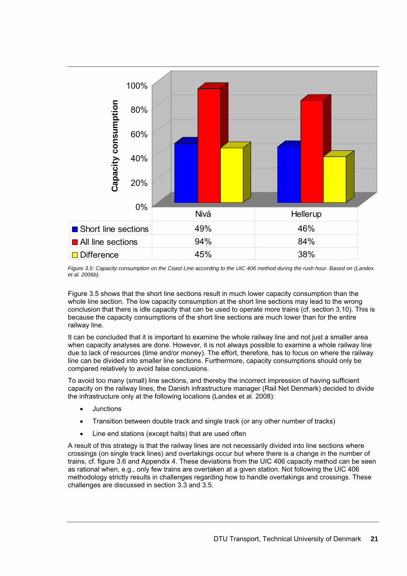
DTU Transport, Technical University of Denmark 21
0%
20%
40%
60%
80%
100%
Cap
acity
con
sum
ptio
n
Short line sections 49% 46%All line sections 94% 84%Difference 45% 38%
Nivå Hellerup
Figure 3.5: Capacity consumption on the Coast Line according to the UIC 406 method during the rush hour. Based on (Landex et al. 2006b).
Figure 3.5 shows that the short line sections result in much lower capacity consumption than the whole line section. The low capacity consumption at the short line sections may lead to the wrong conclusion that there is idle capacity that can be used to operate more trains (cf. section 3.10). This is because the capacity consumptions of the short line sections are much lower than for the entire railway line.
It can be concluded that it is important to examine the whole railway line and not just a smaller area when capacity analyses are done. However, it is not always possible to examine a whole railway line due to lack of resources (time and/or money). The effort, therefore, has to focus on where the railway line can be divided into smaller line sections. Furthermore, capacity consumptions should only be compared relatively to avoid false conclusions.
To avoid too many (small) line sections, and thereby the incorrect impression of having sufficient capacity on the railway lines, the Danish infrastructure manager (Rail Net Denmark) decided to divide the infrastructure only at the following locations (Landex et al. 2008):
• Junctions
• Transition between double track and single track (or any other number of tracks)
• Line end stations (except halts) that are used often
A result of this strategy is that the railway lines are not necessarily divided into line sections where crossings (on single track lines) and overtakings occur but where there is a change in the number of trains, cf. figure 3.6 and Appendix 4. These deviations from the UIC 406 capacity method can be seen as rational when, e.g., only few trains are overtaken at a given station. Not following the UIC 406 methodology strictly results in challenges regarding how to handle overtakings and crossings. These challenges are discussed in section 3.3 and 3.5.
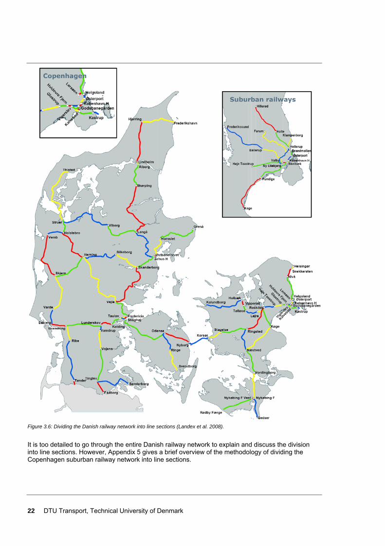
22 DTU Transport, Technical University of Denmark
Figure 3.6: Dividing the Danish railway network into line sections (Landex et al. 2008).
It is too detailed to go through the entire Danish railway network to explain and discuss the division into line sections. However, Appendix 5 gives a brief overview of the methodology of dividing the Copenhagen suburban railway network into line sections.

DTU Transport, Technical University of Denmark 23
3.2.1 Line end stations on open line Sometimes trains are scheduled to turn around on the open line instead of at a station. The reason being that the operator has seen the possibility to use a long layover time to service the next halt but without enough time to run the trains all the way to the next station. This means that the trains turn around on the open line. In these cases, the railway line should not be divided into line sections since the capacity would then be calculated as too low. This is because it would seemingly be possible to compress the timetable graphs more than is actually the case cf. figure 3.7.
Station A Halt B Station C
Distance
Time
Station A Halt B
Distance
Time
Station C
Distance
Time Figure 3.7: Train turning around on open (single track) line – e.g. the halt Exhibition Centre Herning in Denmark. Based on (Landex et al. 2008).
Not dividing railway lines into line sections at halts where the trains turn around has the advantage of it being easier to compare capacity consumptions over time. This is because the paradox situation where fewer trains on the railway line would result in higher capacity consumption (and vice-versa) is avoided.
EXAMPLE In Denmark, there are halts where (some) trains turn around at Vejle Sygehus (Vejle Hospital) on the railway line between Vejle and Herning and Herning Messecenter (Exhibition Centre Herning) on the railway line between Herning and Skjern (DSB 2007). To avoid too low capacity consumptions of these railway lines, it has been decided not to divide the railway lines at Vejle Sygehus and Herning Messecenter8.
In the future, Vejle Sygehus might not be a line end station because few passengers use the halt. Instead, other stations/halts may become new line end stations. One possibility of a halt that can become a new line end station is Odense Sygehus (Odense Hospital) on the railway line between Odense and Svendborg. Here it is possible to offer a better service to the passengers without using extra rolling stock, cf. the timetable example in table 3.1. Table 3.1: Extract from the fixed interval timetable between Odense and Svendborg (DSB 2007) with additional train (red and bold).
Station\Train route T1 T2 T3 T4 Station\Train route T1 T2 T3 T4 Odense 24 38 08 45 Ringe 57 53 17 Odense Sygehus 28 | 12 49 Pederstrup 01 | | Fruens Bøge 31 | 15 Årslev 04 | 23 Hjallese 33 | | Højby 08 | | Højby 37 | | Hjallelse 12 | | Årslev 41 | 23 Fruens Bøge 15 | | Pederstrup 44 | | Odense Sygehus 17 | 30 55Ringe 49 54 29 Odense 21 08 33 58
Changing the timetable as suggested in table 3.1 would not change the division of the railway line into line sections as Odense Sygehus is a halt. However, if enough time was available to run to Fruens 8 The railway lines are divided at the nearby junctions of Vejle and Herning.
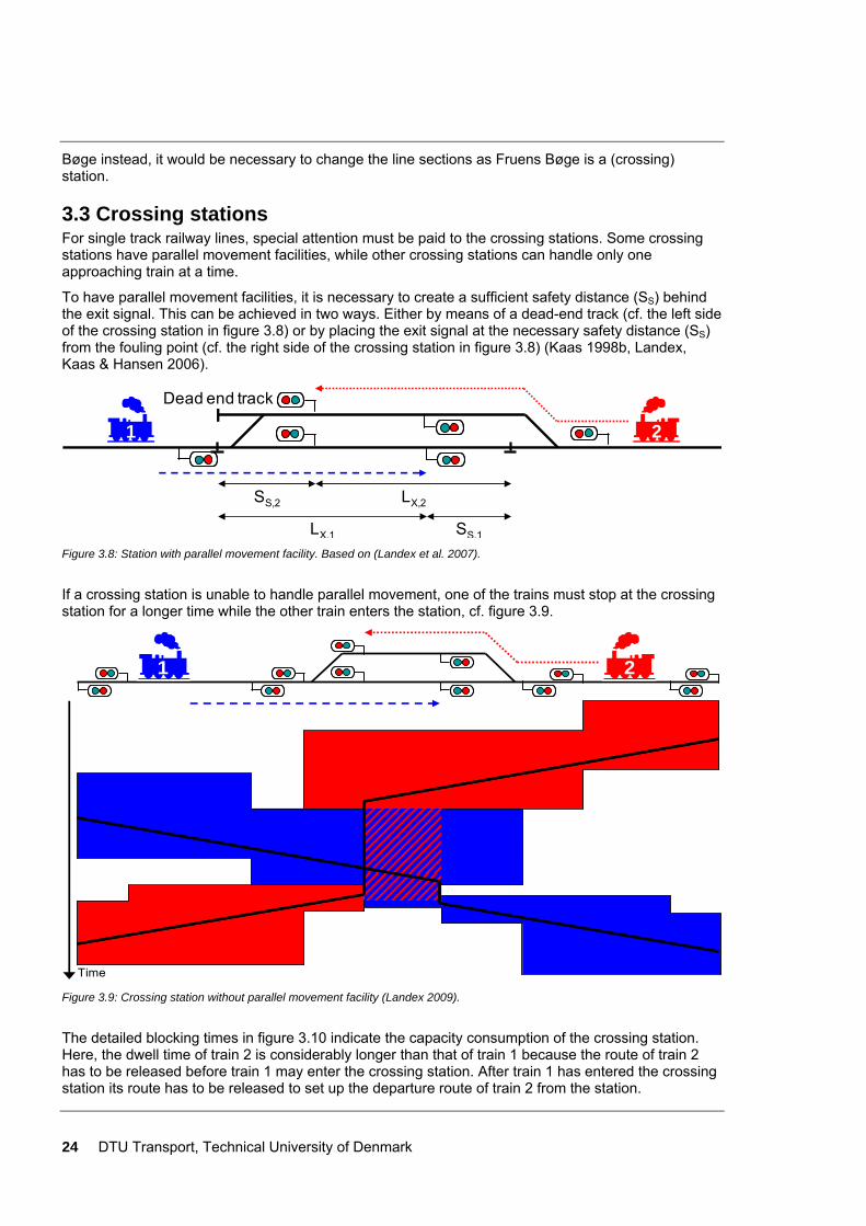
24 DTU Transport, Technical University of Denmark
Bøge instead, it would be necessary to change the line sections as Fruens Bøge is a (crossing) station.
3.3 Crossing stations For single track railway lines, special attention must be paid to the crossing stations. Some crossing stations have parallel movement facilities, while other crossing stations can handle only one approaching train at a time.
To have parallel movement facilities, it is necessary to create a sufficient safety distance (SS) behind the exit signal. This can be achieved in two ways. Either by means of a dead-end track (cf. the left side of the crossing station in figure 3.8) or by placing the exit signal at the necessary safety distance (SS) from the fouling point (cf. the right side of the crossing station in figure 3.8) (Kaas 1998b, Landex, Kaas & Hansen 2006).
LX,2SS,2
LX,1 SS,1
1 2
Dead end track
Figure 3.8: Station with parallel movement facility. Based on (Landex et al. 2007).
If a crossing station is unable to handle parallel movement, one of the trains must stop at the crossing station for a longer time while the other train enters the station, cf. figure 3.9.
11 22
Time Figure 3.9: Crossing station without parallel movement facility (Landex 2009).
The detailed blocking times in figure 3.10 indicate the capacity consumption of the crossing station. Here, the dwell time of train 2 is considerably longer than that of train 1 because the route of train 2 has to be released before train 1 may enter the crossing station. After train 1 has entered the crossing station its route has to be released to set up the departure route of train 2 from the station.
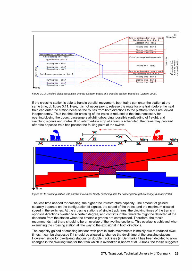
DTU Transport, Technical University of Denmark 25
Time for setting up train route – train 2Signal realizing time – train 2
Approach time – train 2
Running time – train 2
Clearing time – train 2Release time – train 2
End of passenger exchange – train 2
Waiting time – train 2
Signal realizing time – train 2Running time – train 2Clearing time – train 2Release time – train 2
Time for setting up train route – train 2
Time for setting up train route – train 1Signal realizing time – train 1
Approach time – train 1
Running time – train 1
End of passenger exchange – train 1
Running time – train 1Clearing time – train 1Release time – train 1
Clearing time – train 1Release time – train 1
Dw
ell t
ime
Dw
ell t
ime
Ext
ra d
wel
l tim
edu
e to
no
para
llel
mov
emen
t fac
ility
Time
Distance
Figure 3.10: Detailed block occupation time for platform tracks of a crossing station. Based on (Landex 2009).
If the crossing station is able to handle parallel movement, both trains can enter the station at the same time, cf. figure 3.11. Here, it is not necessary to release the route for one train before the next train can enter the station because the routes from both directions to the platform tracks are locked independently. Thus the time for crossing of the trains is reduced to the time necessary for opening/closing the doors, passengers alighting/boarding, possible (un)loading of freight, and switching signals and routes. If no intermediate stop of a train is scheduled, the trains may proceed after the opposite train has passed the fouling point of the switch.
11 22
Time Figure 3.11: Crossing station with parallel movement facility (including stop for passenger/freight exchange) (Landex 2009).
The less time needed for crossing, the higher the infrastructure capacity. The amount of gained capacity depends on the configuration of signals, the speed of the trains, and the maximum allowed speed in the switches. At the crossing stations of single track lines, the blocking times of the trains in opposite directions overlap to a certain degree, and conflicts in the timetable might be detected at the departure from the station when the timetable graphs are compressed. Therefore, the thesis recommends that there should to be an overlap of the two line sections. This overlap is achieved when examining the crossing station all the way to the exit signal in both directions.
The capacity gained at crossing stations with parallel train movements is mainly due to reduced dwell times. It can be discussed if it should be allowed to change the dwell time at the crossing stations. However, since for overtaking stations on double track lines (in Denmark) it has been decided to allow changes in the dwelling time for the train which is overtaken (Landex et al. 2006a), the thesis suggests
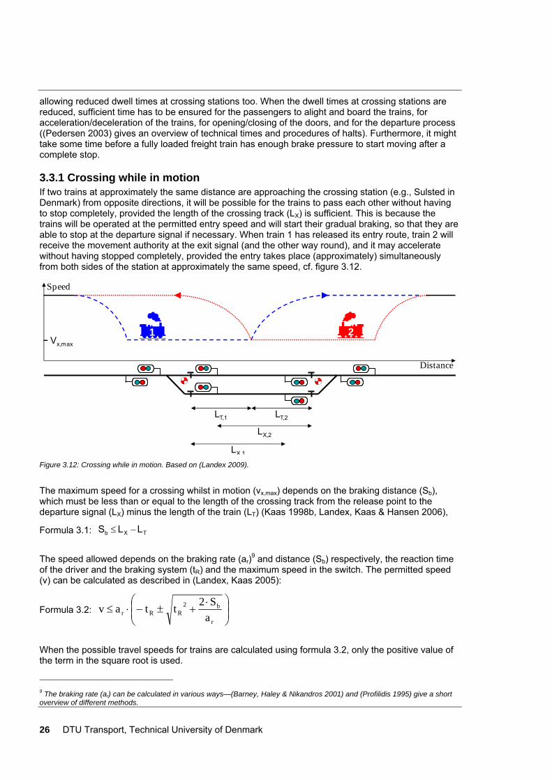
26 DTU Transport, Technical University of Denmark
allowing reduced dwell times at crossing stations too. When the dwell times at crossing stations are reduced, sufficient time has to be ensured for the passengers to alight and board the trains, for acceleration/deceleration of the trains, for opening/closing of the doors, and for the departure process ((Pedersen 2003) gives an overview of technical times and procedures of halts). Furthermore, it might take some time before a fully loaded freight train has enough brake pressure to start moving after a complete stop.
3.3.1 Crossing while in motion If two trains at approximately the same distance are approaching the crossing station (e.g., Sulsted in Denmark) from opposite directions, it will be possible for the trains to pass each other without having to stop completely, provided the length of the crossing track (LX) is sufficient. This is because the trains will be operated at the permitted entry speed and will start their gradual braking, so that they are able to stop at the departure signal if necessary. When train 1 has released its entry route, train 2 will receive the movement authority at the exit signal (and the other way round), and it may accelerate without having stopped completely, provided the entry takes place (approximately) simultaneously from both sides of the station at approximately the same speed, cf. figure 3.12.
Distance
Speed
LT,1 LT,2
21Vx,max
LX,2
LX,1 Figure 3.12: Crossing while in motion. Based on (Landex 2009).
The maximum speed for a crossing whilst in motion (vx,max) depends on the braking distance (Sb), which must be less than or equal to the length of the crossing track from the release point to the departure signal (LX) minus the length of the train (LT) (Kaas 1998b, Landex, Kaas & Hansen 2006),
Formula 3.1: TXb LLS −≤
The speed allowed depends on the braking rate (ar)9 and distance (Sb) respectively, the reaction time of the driver and the braking system (tR) and the maximum speed in the switch. The permitted speed (v) can be calculated as described in (Landex, Kaas 2005):
Formula 3.2: ⎟⎟⎠
⎞⎜⎜⎝
⎛ ⋅+±−⋅≤
r
b2RRr a
S2ttav
When the possible travel speeds for trains are calculated using formula 3.2, only the positive value of the term in the square root is used.
9 The braking rate (ar) can be calculated in various ways—(Barney, Haley & Nikandros 2001) and (Profilidis 1995) give a short overview of different methods.
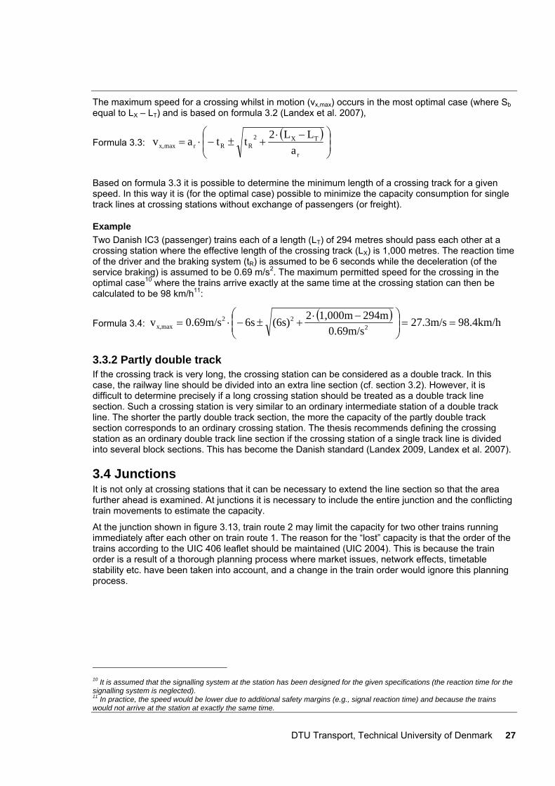
DTU Transport, Technical University of Denmark 27
The maximum speed for a crossing whilst in motion (vx,max) occurs in the most optimal case (where Sb equal to LX – LT) and is based on formula 3.2 (Landex et al. 2007),
Formula 3.3: ( )
⎟⎟⎠
⎞⎜⎜⎝
⎛ −⋅+±−⋅=
r
TX2RRrmaxx, a
LL2ttav
Based on formula 3.3 it is possible to determine the minimum length of a crossing track for a given speed. In this way it is (for the optimal case) possible to minimize the capacity consumption for single track lines at crossing stations without exchange of passengers (or freight).
Example Two Danish IC3 (passenger) trains each of a length (LT) of 294 metres should pass each other at a crossing station where the effective length of the crossing track (LX) is 1,000 metres. The reaction time of the driver and the braking system (tR) is assumed to be 6 seconds while the deceleration (of the service braking) is assumed to be 0.69 m/s2. The maximum permitted speed for the crossing in the optimal case10 where the trains arrive exactly at the same time at the crossing station can then be calculated to be 98 km/h11:
Formula 3.4: ( ) .4km/h893m/s.27
0.69m/s294m1,000m2(6s)6s0.69m/sv 2
22maxx, ==⎟⎟
⎠
⎞⎜⎜⎝
⎛ −⋅+±−⋅=
3.3.2 Partly double track If the crossing track is very long, the crossing station can be considered as a double track. In this case, the railway line should be divided into an extra line section (cf. section 3.2). However, it is difficult to determine precisely if a long crossing station should be treated as a double track line section. Such a crossing station is very similar to an ordinary intermediate station of a double track line. The shorter the partly double track section, the more the capacity of the partly double track section corresponds to an ordinary crossing station. The thesis recommends defining the crossing station as an ordinary double track line section if the crossing station of a single track line is divided into several block sections. This has become the Danish standard (Landex 2009, Landex et al. 2007).
3.4 Junctions It is not only at crossing stations that it can be necessary to extend the line section so that the area further ahead is examined. At junctions it is necessary to include the entire junction and the conflicting train movements to estimate the capacity.
At the junction shown in figure 3.13, train route 2 may limit the capacity for two other trains running immediately after each other on train route 1. The reason for the “lost” capacity is that the order of the trains according to the UIC 406 leaflet should be maintained (UIC 2004). This is because the train order is a result of a thorough planning process where market issues, network effects, timetable stability etc. have been taken into account, and a change in the train order would ignore this planning process.
10 It is assumed that the signalling system at the station has been designed for the given specifications (the reaction time for the signalling system is neglected). 11 In practice, the speed would be lower due to additional safety margins (e.g., signal reaction time) and because the trains would not arrive at the station at exactly the same time.
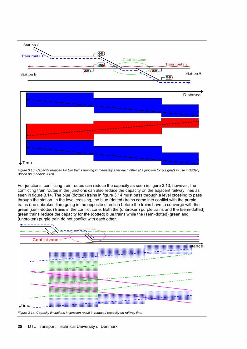
28 DTU Transport, Technical University of Denmark
Distance
Time
Conflict zoneTrain route 1
Train route 2
Station A
Station C
Station B
Figure 3.13: Capacity reduced for two trains running immediately after each other at a junction (only signals in use included). Based on (Landex 2009).
For junctions, conflicting train routes can reduce the capacity as seen in figure 3.13; however, the conflicting train routes in the junctions can also reduce the capacity on the adjacent railway lines as seen in figure 3.14. The blue (dotted) trains in figure 3.14 must pass through a level crossing to pass through the station. In the level crossing, the blue (dotted) trains come into conflict with the purple trains (the unbroken line) going in the opposite direction before the trains have to converge with the green (semi-dotted) trains in the conflict zone. Both the (unbroken) purple trains and the (semi-dotted) green trains reduce the capacity for the (dotted) blue trains while the (semi-dotted) green and (unbroken) purple train do not conflict with each other.
Conflict zone
Time
Distance
Figure 3.14: Capacity limitations in junction result in reduced capacity on railway line.
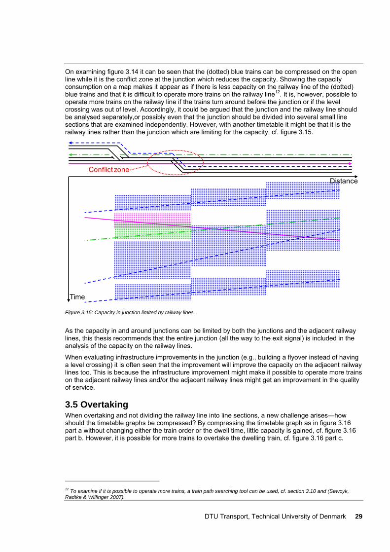
DTU Transport, Technical University of Denmark 29
On examining figure 3.14 it can be seen that the (dotted) blue trains can be compressed on the open line while it is the conflict zone at the junction which reduces the capacity. Showing the capacity consumption on a map makes it appear as if there is less capacity on the railway line of the (dotted) blue trains and that it is difficult to operate more trains on the railway line12. It is, however, possible to operate more trains on the railway line if the trains turn around before the junction or if the level crossing was out of level. Accordingly, it could be argued that the junction and the railway line should be analysed separately,or possibly even that the junction should be divided into several small line sections that are examined independently. However, with another timetable it might be that it is the railway lines rather than the junction which are limiting for the capacity, cf. figure 3.15.
Conflict zone
Time
Distance
Figure 3.15: Capacity in junction limited by railway lines.
As the capacity in and around junctions can be limited by both the junctions and the adjacent railway lines, this thesis recommends that the entire junction (all the way to the exit signal) is included in the analysis of the capacity on the railway lines.
When evaluating infrastructure improvements in the junction (e.g., building a flyover instead of having a level crossing) it is often seen that the improvement will improve the capacity on the adjacent railway lines too. This is because the infrastructure improvement might make it possible to operate more trains on the adjacent railway lines and/or the adjacent railway lines might get an improvement in the quality of service.
3.5 Overtaking When overtaking and not dividing the railway line into line sections, a new challenge arises—how should the timetable graphs be compressed? By compressing the timetable graph as in figure 3.16 part a without changing either the train order or the dwell time, little capacity is gained, cf. figure 3.16 part b. However, it is possible for more trains to overtake the dwelling train, cf. figure 3.16 part c.
12 To examine if it is possible to operate more trains, a train path searching tool can be used, cf. section 3.10 and (Sewcyk, Radtke & Wilfinger 2007).

30 DTU Transport, Technical University of Denmark
b
d
a
cTime
Time
Time
Time
DistanceDistance
DistanceDistance
Figure 3.16: Timetable compression when overtaking. Based on (Landex et al. 2006a).
If the timetable is changed to allow more trains than timetabled to overtake a train at a station (part c in figure 3.16), the train order is changed at the end of the line section. This can result in new conflicts outside the analysis area (or line section) if, for instance, no timetable slot is available. Therefore, the train order should remain fixed when compressing the timetable graphs.
Instead of changing the order of the trains (by having more trains overtaking a train), the dwell time of the train that is overtaken can be reduced, cf. figure 3.16 part d. However, it should be noted that it may take some time before a fully loaded freight train has sufficient brake pressure to start moving after a complete halt, and that passengers need sufficient time to alight and board the passenger train (an overview of the dwelling time for passenger trains can be seen in (Pedersen 2003)). The thesis suggests allowing reduced dwell time for the train that is overtaken providing the minimum dwell time for the train is not exceeded. This recommendation has now become the Danish standard (Landex et al. 2006b).
3.6 Line end stations Similar to crossing stations, junctions and overtaking stations, special attention has to be paid to line end stations. Trains turning around have long dwell times that can block the train path for the following train. To include the layover time, the thesis recommends examining the arriving train until it passes the exit signal on its way out of the line end station or it arrives at the depot. In this way, both the layover time and the possible conflicts at the switch zone(s) are included in the analysis.
Due to the blocked avoiding track, there is a limit to how much the timetable graphs can be compressed. However, trains often dwell for longer than necessary at the avoiding track due to recovery and/or to fit into the right train path. Therefore, the thesis suggests that only the minimum dwell/layover time on the avoiding track (and the train order) should be considered when compressing the timetable graphs (this includes the time buffers agreed upon with the train operating company), cf. figure 3.17.
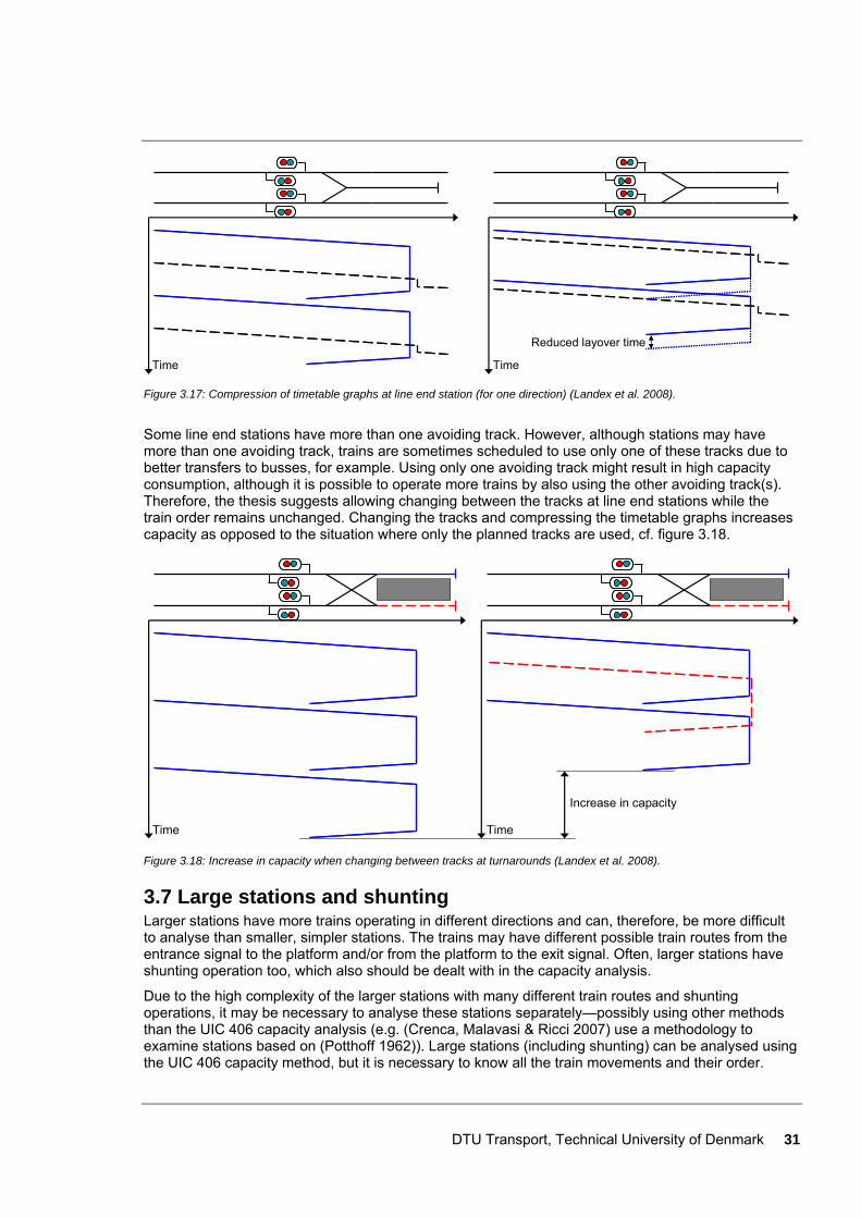
DTU Transport, Technical University of Denmark 31
Reduced layover time
TimeTime Figure 3.17: Compression of timetable graphs at line end station (for one direction) (Landex et al. 2008).
Some line end stations have more than one avoiding track. However, although stations may have more than one avoiding track, trains are sometimes scheduled to use only one of these tracks due to better transfers to busses, for example. Using only one avoiding track might result in high capacity consumption, although it is possible to operate more trains by also using the other avoiding track(s). Therefore, the thesis suggests allowing changing between the tracks at line end stations while the train order remains unchanged. Changing the tracks and compressing the timetable graphs increases capacity as opposed to the situation where only the planned tracks are used, cf. figure 3.18.
Increase in capacity
TimeTime
Figure 3.18: Increase in capacity when changing between tracks at turnarounds (Landex et al. 2008).
3.7 Large stations and shunting Larger stations have more trains operating in different directions and can, therefore, be more difficult to analyse than smaller, simpler stations. The trains may have different possible train routes from the entrance signal to the platform and/or from the platform to the exit signal. Often, larger stations have shunting operation too, which also should be dealt with in the capacity analysis.
Due to the high complexity of the larger stations with many different train routes and shunting operations, it may be necessary to analyse these stations separately—possibly using other methods than the UIC 406 capacity analysis (e.g. (Crenca, Malavasi & Ricci 2007) use a methodology to examine stations based on (Potthoff 1962)). Large stations (including shunting) can be analysed using the UIC 406 capacity method, but it is necessary to know all the train movements and their order.
32 DTU Transport, Technical University of Denmark
However, it may not be possible to know the exact train movements for large stations as there are many shunting operations such as:
• Shunting between platform and depot tracks
• Attaching and/or decoupling of train units at the platform track
• Shunting operation at the depot that blocks a main track or train routes in the switch zone
• Shunting from platform track to maintenance and/or cleaning facilities
Typically, the shunting operations vary during the day and over time—some shunting movements may not even be planned13 due to break down in rolling stock, for example, or cancelations due to delays. Consequently, it is difficult to predict the number of shunting operations at the larger stations. Furthermore, some of the “non-critical” shunting movements may be allowed only in non-critical periods.
Due to the complexity of the larger stations and the shunting movements, great care must be taken when analysing these stations. A simple approach is to analyse only the scheduled trains and the known shunting and to include a higher quality factor14 or another type of supplement. This implicitly takes into account the necessity of reserving extra time in the timetable for shunting operation.
As most of the shunting operations are planned (in detail) after the public timetable has been finalised, they are adapted to fit in with the fixed schedule. In the case of delays, the shunting operation adapts to the realized timetable as far as possible and with as little disturbance as possible to trains. This means that the shunting operation strives to use the “idle capacity” within the station for its operation. Therefore, the “time slots” for the shunting operations can be changed to some extent, which makes it even more difficult to use the UIC 406 capacity method strictly. The thesis, therefore, suggests that the larger stations with many shunting movements are analysed with a higher quality factor or another type of supplement along with the UIC 406 capacity method.
In Denmark, there are few large stations with many shunting operations, and it can be discussed whether there are stations apart from Copenhagen and Århus central stations that are sufficiently complex to warrant being analysed separately.
3.8 Changing between tracks at stations and at lines with more than two tracks Railway lines with three or more tracks are generally not modelled. Instead, they are divided into several lines with a maximum of two tracks (Oetting 2007). If tracks are used for running some train routes separately from others, the tracks used for each group of train routes can also be analysed separately. However, since line sections with four tracks are often used for one-direction running where fast trains can overtake slower trains, there is a risk of additional overtakings when compressing the timetable graph (cf. figure 3.19 part a and c). Therefore, in the Danish way of using the UIC 406 method for capacity analysis, it has been decided that the train order must remain unchanged in both ends of the line section in cases of one-direction operation (cf. figure 3.19 part a and b) (Landex et al. 2006a, Landex et al. 2006b). The train order has to remain the same due to the limitations of the infrastructure and timetable outside the analysis area—the so-called network effects (Hansen 2004b, Hansen, Landex & Kaas 2006, Landex, Kaas & Hansen 2006).
13 No models are able to analyse the exact consequences of unscheduled shunting. 14 For more information about the quality factor see section 5.3.
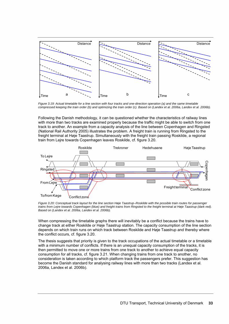
DTU Transport, Technical University of Denmark 33
a b c
Distance DistanceDistance
Time TimeTime
Figure 3.19: Actual timetable for a line section with four tracks and one-direction operation (a) and the same timetable compressed keeping the train order (b) and optimizing the train order (c). Based on (Landex et al. 2006a, Landex et al. 2006b).
Following the Danish methodology, it can be questioned whether the characteristics of railway lines with more than two tracks are examined properly because the traffic might be able to switch from one track to another. An example from a capacity analysis of the line between Copenhagen and Ringsted (National Rail Authority 2005) illustrates the problem. A freight train is running from Ringsted to the freight terminal at Høje Taastrup. Simultaneously with the freight train passing Roskilde, a regional train from Lejre towards Copenhagen leaves Roskilde, cf. figure 3.20.
Freight terminal
Roskilde Trekroner Hedehusene Høje Taastrup
To/from Køge
From Lejre
To Lejre
Ringsted
Copenhagen
Conflict zone
Conflict zone
Figure 3.20: Conceptual track layout for the line section Høje Taastrup–Roskilde with the possible train routes for passenger trains from Lejre towards Copenhagen (blue) and freight trains from Ringsted to the freight terminal at Høje Taastrup (dark red). Based on (Landex et al. 2006a, Landex et al. 2006b).
When compressing the timetable graphs there will inevitably be a conflict because the trains have to change track at either Roskilde or Høje Taastrup station. The capacity consumption of the line section depends on which train runs on which track between Roskilde and Høje Taastrup and thereby where the conflict occurs, cf. figure 3.20.
The thesis suggests that priority is given to the track occupations of the actual timetable or a timetable with a minimum number of conflicts. If there is an unequal capacity consumption of the tracks, it is then permitted to move one or more trains from one track to another to achieve equal capacity consumption for all tracks, cf. figure 3.21. When changing trains from one track to another, no consideration is taken according to which platform track the passengers prefer. This suggestion has become the Danish standard for analysing railway lines with more than two tracks (Landex et al. 2006a, Landex et al. 2006b).

34 DTU Transport, Technical University of Denmark
Divide into line sections
Compress the timetable graph
Work out capacity consumption for each line section
Large difference in capacity consumption for the tracks
Change track for train(s) Capacity consumption of line section
NoYes
Divide into line sections
Compress the timetable graph
Work out capacity consumption for each line section
Large difference in capacity consumption for the tracks
Change track for train(s) Capacity consumption of line section
NoYes
Figure 3.21: Changing between tracks on railway lines with more than two tracks.
A situation similar to the track section with four tracks can be found when two double track railway lines run parallel, cf. figure 3.22. When the UIC 406 method is followed stringently the infrastructure should be divided in two line sections A-C-B and A-D-B. However, if line sections A-C-B and A-D-B are separated only by a short distance, it will be obvious to examine them as one track section with four tracks as described above.
A
C
D
B
Figure 3.22: Infrastructure for two (double track) line sections running parallel (Landex et al. 2006a).
If the four tracks in figure 3.22 are separated so that C and D represent two different cities, the analysis should normally be done on two different line sections, A-C-B and A-D-B, each with double track. Nevertheless, if the overall capacity between A and B is to be evaluated, it could be useful to evaluate the network as a line section with four tracks. By evaluating the network as a line section with four tracks, it is possible to move through-going trains (no stop between A and B) from one track to another to achieve equal capacity consumption and thereby evaluate the overall capacity between A and B.
When evaluating the overall capacity between A and B in figure 3.22 it might be necessary to compromise the principles of the UIC 406 method. For example, if some trains turn around at station C, the line section ought to be divided at station C. When dividing one line section into several smaller line sections, it becomes difficult to compare the capacity consumption of the two lines (A-C-B and A-D-B) as the capacity consumption depends on the length of the line sections examined (cf. section
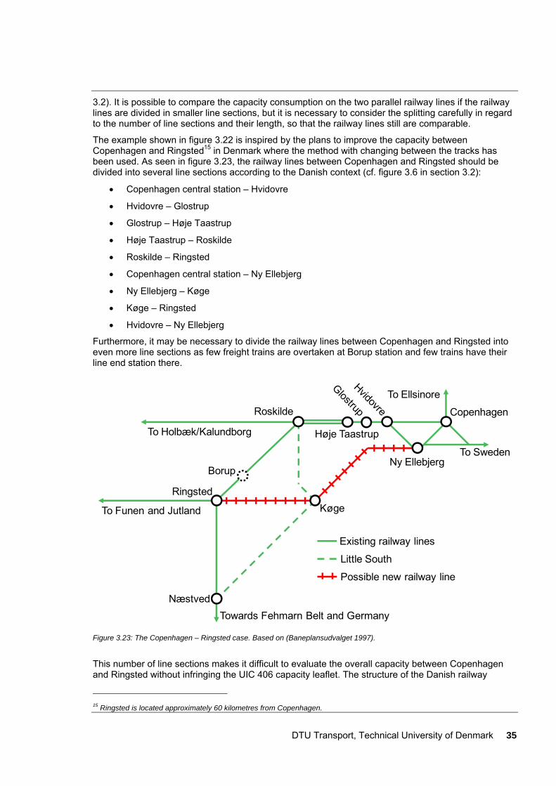
DTU Transport, Technical University of Denmark 35
3.2). It is possible to compare the capacity consumption on the two parallel railway lines if the railway lines are divided in smaller line sections, but it is necessary to consider the splitting carefully in regard to the number of line sections and their length, so that the railway lines still are comparable.
The example shown in figure 3.22 is inspired by the plans to improve the capacity between Copenhagen and Ringsted15 in Denmark where the method with changing between the tracks has been used. As seen in figure 3.23, the railway lines between Copenhagen and Ringsted should be divided into several line sections according to the Danish context (cf. figure 3.6 in section 3.2):
• Copenhagen central station – Hvidovre
• Hvidovre – Glostrup
• Glostrup – Høje Taastrup
• Høje Taastrup – Roskilde
• Roskilde – Ringsted
• Copenhagen central station – Ny Ellebjerg
• Ny Ellebjerg – Køge
• Køge – Ringsted
• Hvidovre – Ny Ellebjerg
Furthermore, it may be necessary to divide the railway lines between Copenhagen and Ringsted into even more line sections as few freight trains are overtaken at Borup station and few trains have their line end station there.
Køge
Næstved
Roskilde
Ny Ellebjerg
Copenhagen
To Sweden
To Holbæk/Kalundborg
To Funen and Jutland
Towards Fehmarn Belt and Germany
Existing railway lines
Little South
Possible new railway line
Ringsted
To Ellsinore
Høje Taastrup
Borup
Figure 3.23: The Copenhagen – Ringsted case. Based on (Baneplansudvalget 1997).
This number of line sections makes it difficult to evaluate the overall capacity between Copenhagen and Ringsted without infringing the UIC 406 capacity leaflet. The structure of the Danish railway
15 Ringsted is located approximately 60 kilometres from Copenhagen.
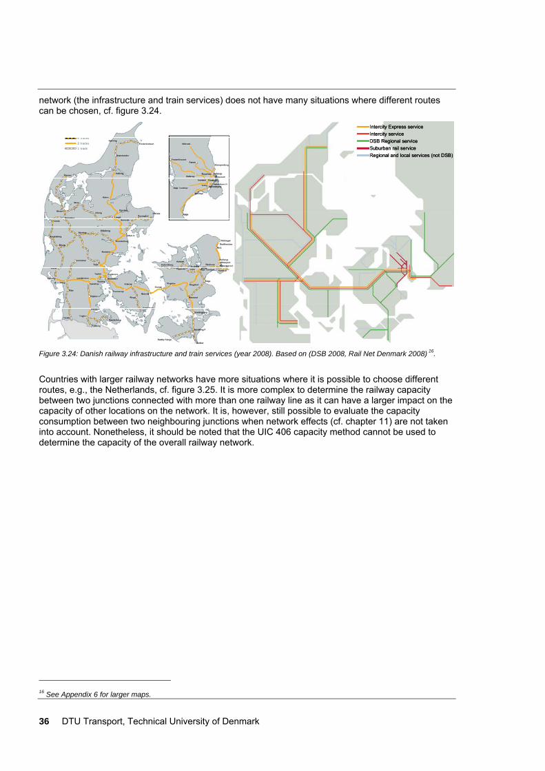
36 DTU Transport, Technical University of Denmark
network (the infrastructure and train services) does not have many situations where different routes can be chosen, cf. figure 3.24.
Intercity Express serviceIntercity serviceDSB Regional serviceSuburban rail serviceRegional and local services (not DSB)
Intercity Express serviceIntercity serviceDSB Regional serviceSuburban rail serviceRegional and local services (not DSB)
Figure 3.24: Danish railway infrastructure and train services (year 2008). Based on (DSB 2008, Rail Net Denmark 2008) 16.
Countries with larger railway networks have more situations where it is possible to choose different routes, e.g., the Netherlands, cf. figure 3.25. It is more complex to determine the railway capacity between two junctions connected with more than one railway line as it can have a larger impact on the capacity of other locations on the network. It is, however, still possible to evaluate the capacity consumption between two neighbouring junctions when network effects (cf. chapter 11) are not taken into account. Nonetheless, it should be noted that the UIC 406 capacity method cannot be used to determine the capacity of the overall railway network.
16 See Appendix 6 for larger maps.
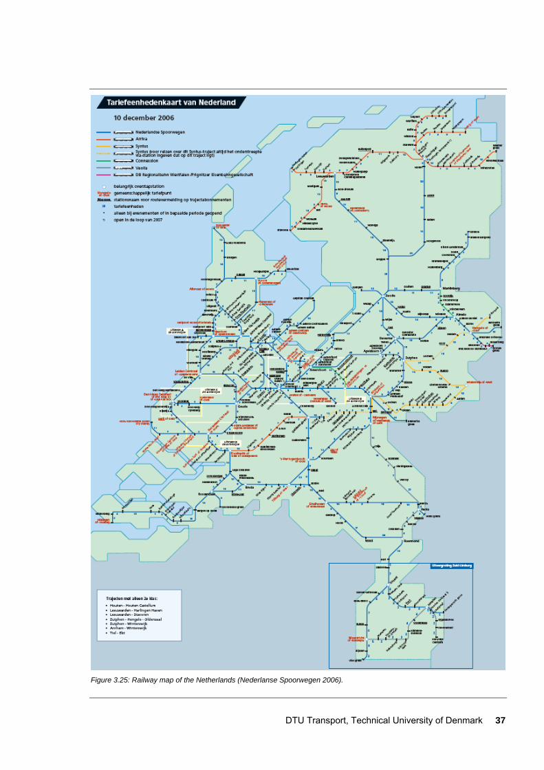
DTU Transport, Technical University of Denmark 37
Figure 3.25: Railway map of the Netherlands (Nederlanse Spoorwegen 2006).
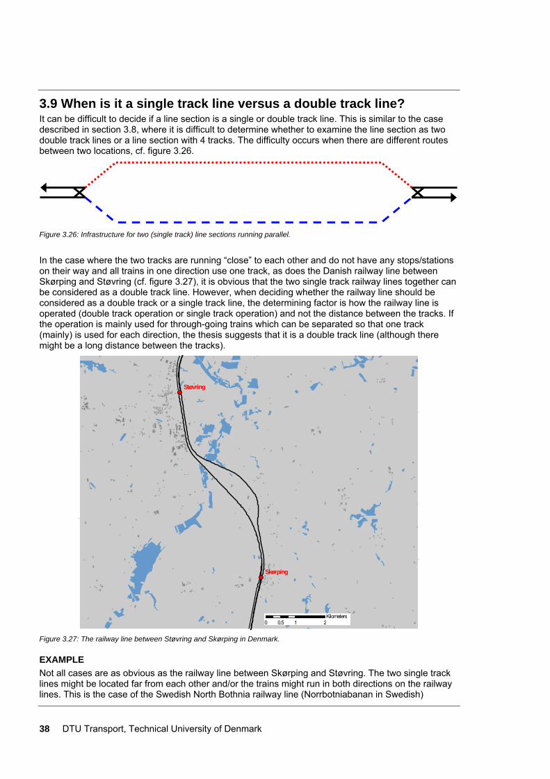
38 DTU Transport, Technical University of Denmark
3.9 When is it a single track line versus a double track line? It can be difficult to decide if a line section is a single or double track line. This is similar to the case described in section 3.8, where it is difficult to determine whether to examine the line section as two double track lines or a line section with 4 tracks. The difficulty occurs when there are different routes between two locations, cf. figure 3.26.
Figure 3.26: Infrastructure for two (single track) line sections running parallel.
In the case where the two tracks are running “close” to each other and do not have any stops/stations on their way and all trains in one direction use one track, as does the Danish railway line between Skørping and Støvring (cf. figure 3.27), it is obvious that the two single track railway lines together can be considered as a double track line. However, when deciding whether the railway line should be considered as a double track or a single track line, the determining factor is how the railway line is operated (double track operation or single track operation) and not the distance between the tracks. If the operation is mainly used for through-going trains which can be separated so that one track (mainly) is used for each direction, the thesis suggests that it is a double track line (although there might be a long distance between the tracks).
0 1 20.5Kilometers
Støvring
Skørping
0 1 20.5Kilometers
Figure 3.27: The railway line between Støvring and Skørping in Denmark.
EXAMPLE Not all cases are as obvious as the railway line between Skørping and Støvring. The two single track lines might be located far from each other and/or the trains might run in both directions on the railway lines. This is the case of the Swedish North Bothnia railway line (Norrbotniabanan in Swedish)
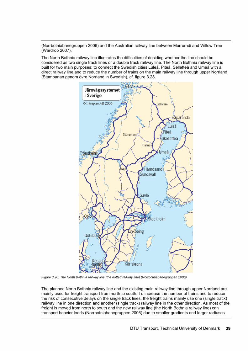
DTU Transport, Technical University of Denmark 39
(Norrbotniabanegruppen 2006) and the Australian railway line between Murrurndi and Willow Tree (Wardrop 2007).
The North Bothnia railway line illustrates the difficulties of deciding whether the line should be considered as two single track lines or a double track railway line. The North Bothnia railway line is built for two main purposes: to connect the Swedish cities Luleå, Piteå, Sellefteå and Umeå with a direct railway line and to reduce the number of trains on the main railway line through upper Norrland (Stambanan genom övre Norrland in Swedish), cf. figure 3.28.
Figure 3.28: The North Bothnia railway line (the dotted railway line) (Norrbotniabanegruppen 2006).
The planned North Bothnia railway line and the existing main railway line through upper Norrland are mainly used for freight transport from north to south. To increase the number of trains and to reduce the risk of consecutive delays on the single track lines, the freight trains mainly use one (single track) railway line in one direction and another (single track) railway line in the other direction. As most of the freight is moved from north to south and the new railway line (the North Bothnia railway line) can transport heavier loads (Norrbotniabanegruppen 2006) due to smaller gradients and larger radiuses
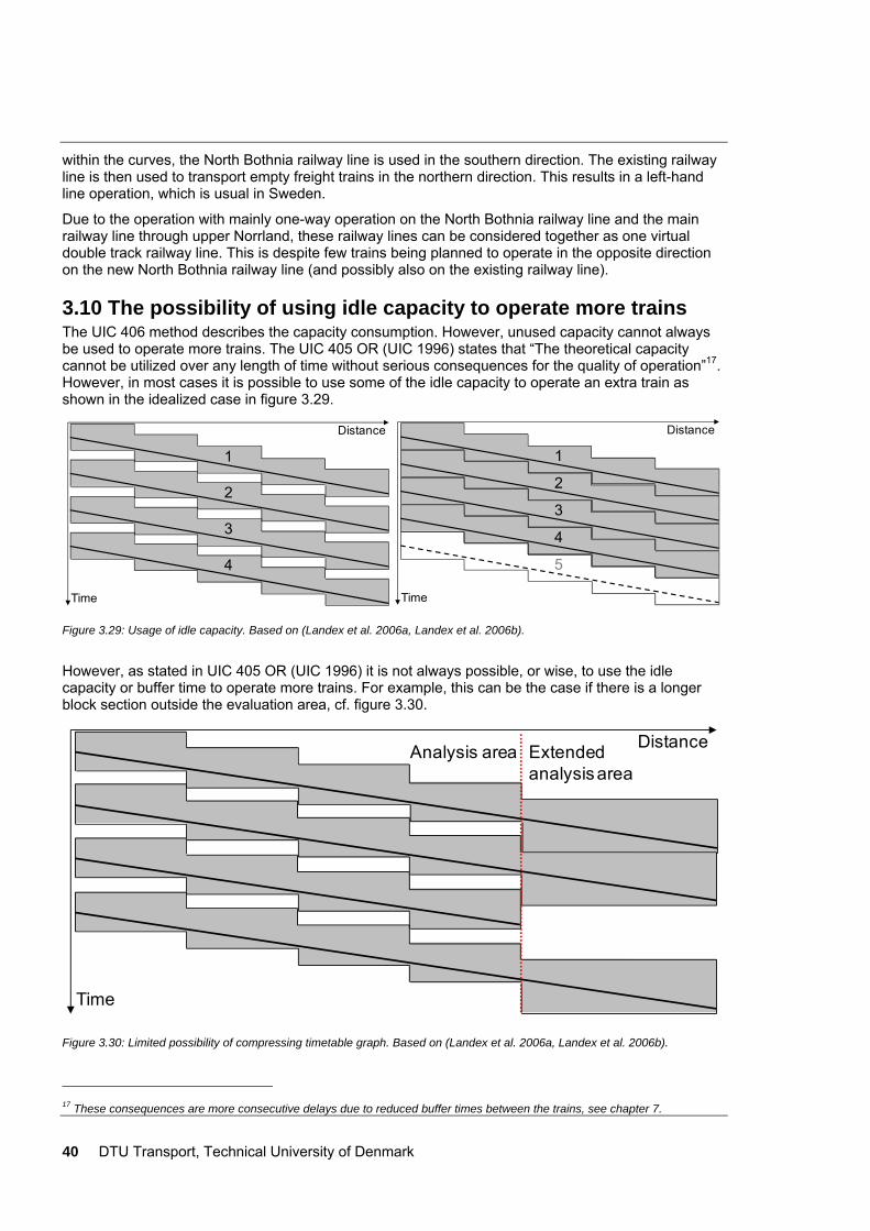
40 DTU Transport, Technical University of Denmark
within the curves, the North Bothnia railway line is used in the southern direction. The existing railway line is then used to transport empty freight trains in the northern direction. This results in a left-hand line operation, which is usual in Sweden.
Due to the operation with mainly one-way operation on the North Bothnia railway line and the main railway line through upper Norrland, these railway lines can be considered together as one virtual double track railway line. This is despite few trains being planned to operate in the opposite direction on the new North Bothnia railway line (and possibly also on the existing railway line).
3.10 The possibility of using idle capacity to operate more trains The UIC 406 method describes the capacity consumption. However, unused capacity cannot always be used to operate more trains. The UIC 405 OR (UIC 1996) states that “The theoretical capacity cannot be utilized over any length of time without serious consequences for the quality of operation”17. However, in most cases it is possible to use some of the idle capacity to operate an extra train as shown in the idealized case in figure 3.29.
Distance
Time
1
2
3
4
Distance
Time
1
2
3
4
5
Figure 3.29: Usage of idle capacity. Based on (Landex et al. 2006a, Landex et al. 2006b).
However, as stated in UIC 405 OR (UIC 1996) it is not always possible, or wise, to use the idle capacity or buffer time to operate more trains. For example, this can be the case if there is a longer block section outside the evaluation area, cf. figure 3.30.
Distance
Time
Extendedanalysis area
Analysis area
Figure 3.30: Limited possibility of compressing timetable graph. Based on (Landex et al. 2006a, Landex et al. 2006b).
17 These consequences are more consecutive delays due to reduced buffer times between the trains, see chapter 7.
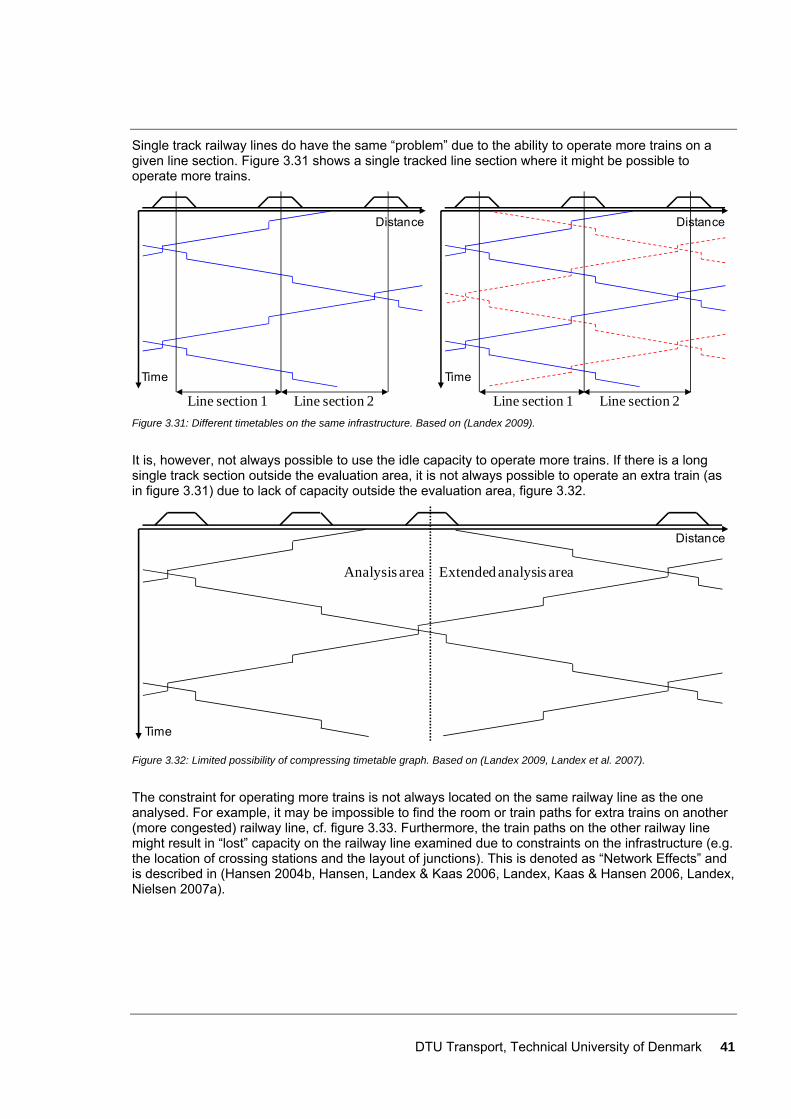
DTU Transport, Technical University of Denmark 41
Single track railway lines do have the same “problem” due to the ability to operate more trains on a given line section. Figure 3.31 shows a single tracked line section where it might be possible to operate more trains.
Line section 1 Line section 2 Line section 1 Line section 2
Time Time
Distance Distance
Figure 3.31: Different timetables on the same infrastructure. Based on (Landex 2009).
It is, however, not always possible to use the idle capacity to operate more trains. If there is a long single track section outside the evaluation area, it is not always possible to operate an extra train (as in figure 3.31) due to lack of capacity outside the evaluation area, figure 3.32.
Analysis area Extended analysis area
Time
Distance
Figure 3.32: Limited possibility of compressing timetable graph. Based on (Landex 2009, Landex et al. 2007).
The constraint for operating more trains is not always located on the same railway line as the one analysed. For example, it may be impossible to find the room or train paths for extra trains on another (more congested) railway line, cf. figure 3.33. Furthermore, the train paths on the other railway line might result in “lost” capacity on the railway line examined due to constraints on the infrastructure (e.g. the location of crossing stations and the layout of junctions). This is denoted as “Network Effects” and is described in (Hansen 2004b, Hansen, Landex & Kaas 2006, Landex, Kaas & Hansen 2006, Landex, Nielsen 2007a).
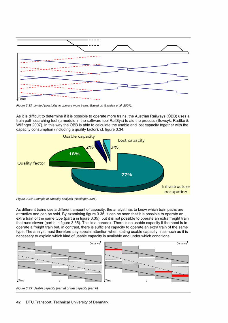
42 DTU Transport, Technical University of Denmark
Time Figure 3.33: Limited possibility to operate more trains. Based on (Landex et al. 2007).
As it is difficult to determine if it is possible to operate more trains, the Austrian Railways (ÖBB) uses a train path searching tool (a module in the software tool RailSys) to aid the process (Sewcyk, Radtke & Wilfinger 2007). In this way the ÖBB is able to calculate the usable and lost capacity together with the capacity consumption (including a quality factor), cf. figure 3.34.
Figure 3.34: Example of capacity analysis (Haslinger 2004).
As different trains use a different amount of capacity, the analyst has to know which train paths are attractive and can be sold. By examining figure 3.35, it can be seen that it is possible to operate an extra train of the same type (part a in figure 3.35), but it is not possible to operate an extra freight train that runs slower (part b in figure 3.35). This is a paradox. There is no usable capacity if the need is to operate a freight train but, in contrast, there is sufficient capacity to operate an extra train of the same type. The analyst must therefore pay special attention when stating usable capacity, inasmuch as it is necessary to explain which kind of usable capacity is available and under which conditions.
aTime
Distance
bTime
Distance
Figure 3.35: Usable capacity (part a) or lost capacity (part b).
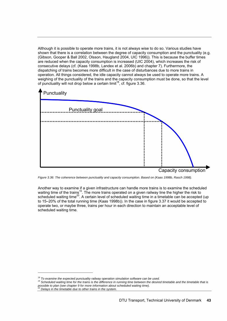
DTU Transport, Technical University of Denmark 43
Although it is possible to operate more trains, it is not always wise to do so. Various studies have shown that there is a correlation between the degree of capacity consumption and the punctuality (e.g. (Gibson, Gooper & Ball 2002, Olsson, Haugland 2004, UIC 1996)). This is because the buffer times are reduced when the capacity consumption is increased (UIC 2004), which increases the risk of consecutive delays (cf. (Kaas 1998b, Landex et al. 2006b) and chapter 7). Furthermore, the dispatching of trains becomes more difficult in the case of disturbances due to more trains in operation. All things considered, the idle capacity cannot always be used to operate more trains. A weighing of the punctuality of the trains and the capacity consumption must be done, so that the level of punctuality will not drop below a certain limit18, cf. figure 3.36.
Capacity consumption
Punctuality
Punctuality goal
Figure 3.36: The coherence between punctuality and capacity consumption. Based on (Kaas 1998b, Rasch 1998).
Another way to examine if a given infrastructure can handle more trains is to examine the scheduled waiting time of the trains19. The more trains operated on a given railway line the higher the risk to scheduled waiting time20. A certain level of scheduled waiting time in a timetable can be accepted (up to 15–20% of the total running time (Kaas 1998b)). In the case in figure 3.37 it would be accepted to operate two, or maybe three, trains per hour in each direction to maintain an acceptable level of scheduled waiting time.
18 To examine the expected punctuality railway operation simulation software can be used. 19 Scheduled waiting time for the trains is the difference in running time between the desired timetable and the timetable that is possible to plan (see chapter 9 for more information about scheduled waiting time). 20 Delays in the timetable due to other trains in the system.
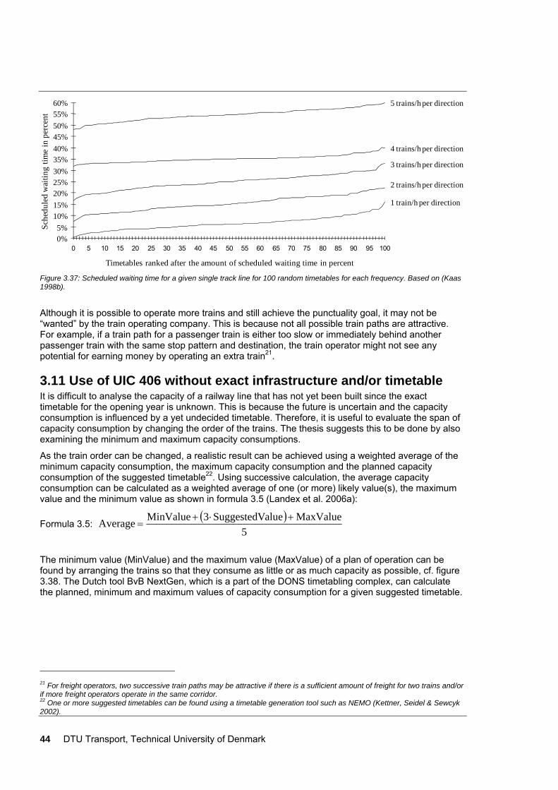
44 DTU Transport, Technical University of Denmark
0%5%
10%15%20%25%30%35%40%45%50%55%60%
0 5 10 15 20 25 30 35 40 45 50 55 60 65 70 75 80 85 90 95 100
Timetables ranked after the amount of scheduled waiting time in percent
Sche
dule
d w
aitin
g tim
e in
per
cent
2 trains/h per direction
5 trains/h per direction
4 trains/h per direction
3 trains/h per direction
1 train/h per direction
Figure 3.37: Scheduled waiting time for a given single track line for 100 random timetables for each frequency. Based on (Kaas 1998b).
Although it is possible to operate more trains and still achieve the punctuality goal, it may not be “wanted” by the train operating company. This is because not all possible train paths are attractive. For example, if a train path for a passenger train is either too slow or immediately behind another passenger train with the same stop pattern and destination, the train operator might not see any potential for earning money by operating an extra train21.
3.11 Use of UIC 406 without exact infrastructure and/or timetable It is difficult to analyse the capacity of a railway line that has not yet been built since the exact timetable for the opening year is unknown. This is because the future is uncertain and the capacity consumption is influenced by a yet undecided timetable. Therefore, it is useful to evaluate the span of capacity consumption by changing the order of the trains. The thesis suggests this to be done by also examining the minimum and maximum capacity consumptions.
As the train order can be changed, a realistic result can be achieved using a weighted average of the minimum capacity consumption, the maximum capacity consumption and the planned capacity consumption of the suggested timetable22. Using successive calculation, the average capacity consumption can be calculated as a weighted average of one (or more) likely value(s), the maximum value and the minimum value as shown in formula 3.5 (Landex et al. 2006a):
Formula 3.5: ( )
5MaxValuealueSuggestedV3MinValueAverage +⋅+
=
The minimum value (MinValue) and the maximum value (MaxValue) of a plan of operation can be found by arranging the trains so that they consume as little or as much capacity as possible, cf. figure 3.38. The Dutch tool BvB NextGen, which is a part of the DONS timetabling complex, can calculate the planned, minimum and maximum values of capacity consumption for a given suggested timetable.
21 For freight operators, two successive train paths may be attractive if there is a sufficient amount of freight for two trains and/or if more freight operators operate in the same corridor. 22 One or more suggested timetables can be found using a timetable generation tool such as NEMO (Kettner, Seidel & Sewcyk 2002).
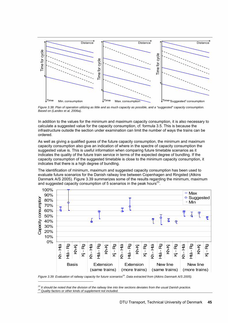
DTU Transport, Technical University of Denmark 45
Tim
e fo
r cyc
le
Tim
e fo
r cyc
le
Tim
e fo
r cyc
le
Min. consumption Max. consumption ”Suggested” consumptionTime
Distance
Time
Distance
Time
Distance
Figure 3.38: Plan of operation utilizing as little and as much capacity as possible, and a “suggested” capacity consumption. Based on (Landex et al. 2006a).
In addition to the values for the minimum and maximum capacity consumption, it is also necessary to calculate a suggested value for the capacity consumption, cf. formula 3.5. This is because the infrastructure outside the section under examination can limit the number of ways the trains can be ordered.
As well as giving a qualified guess of the future capacity consumption, the minimum and maximum capacity consumption also give an indication of where in the spectre of capacity consumption the suggested value is. This is useful information when comparing future timetable scenarios as it indicates the quality of the future train service in terms of the expected degree of bundling. If the capacity consumption of the suggested timetable is close to the minimum capacity consumption, it indicates that there is a high degree of bundling.
The identification of minimum, maximum and suggested capacity consumption has been used to evaluate future scenarios for the Danish railway line between Copenhagen and Ringsted (Atkins Danmark A/S 2005). Figure 3.39 summarizes some of the results regarding the minimum, maximum and suggested capacity consumption of 5 scenarios in the peak hours23.
0%10%20%30%40%50%60%70%80%90%
100%
Kh -
Htå
Htå
- R
g
Kh-K
j
Kj -
Rg
Kh -
Htå
Htå
- R
g
Kh-K
j
Kj -
Rg
Kh -
Htå
Htå
- R
g
Kh-K
j
Kj -
Rg
Kh -
Htå
Htå
- R
g
Kh-K
j
Kj -
Rg
Kh -
Htå
Htå
- R
g
Kh-K
j
Kj -
Rg
Basis Extension(same trains)
Extension(more trains)
New line(same trains)
New line(more trains)
Cap
acity
con
sum
ptio
n
MaxSuggestedMin
Figure 3.39: Evaluation of railway capacity for future scenarios24. Data extracted from (Atkins Danmark A/S 2005). 23 It should be noted that the division of the railway line into line sections deviates from the usual Danish practice. 24 Quality factors or other kinds of supplement not included.
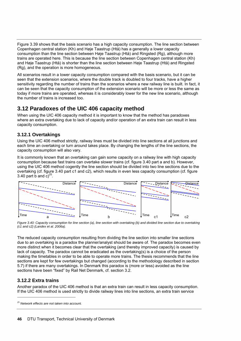
46 DTU Transport, Technical University of Denmark
Figure 3.39 shows that the basis scenario has a high capacity consumption. The line section between Copenhagen central station (Kh) and Høje Taastrup (Htå) has a generally a lower capacity consumption than the line section between Høje Taastrup (Htå) and Ringsted (Rg), although more trains are operated here. This is because the line section between Copenhagen central station (Kh) and Høje Taastrup (Htå) is shorter than the line section between Høje Taastrup (Htå) and Ringsted (Rg), and the operation is more homogeneous.
All scenarios result in a lower capacity consumption compared with the basis scenario, but it can be seen that the extension scenarios, where the double track is doubled to four tracks, have a higher sensitivity regarding the number of trains than the scenarios where a new railway line is built. In fact, it can be seen that the capacity consumption of the extension scenario will be more or less the same as today if more trains are operated, whereas it is considerably lower for the new line scenario, although the number of trains is increased too.
3.12 Paradoxes of the UIC 406 capacity method When using the UIC 406 capacity method it is important to know that the method has paradoxes where an extra overtaking due to lack of capacity and/or operation of an extra train can result in less capacity consumption.
3.12.1 Overtakings Using the UIC 406 method strictly, railway lines must be divided into line sections at all junctions and each time an overtaking or turn around takes place. By changing the lengths of the line sections, the capacity consumption will also vary.
It is commonly known that an overtaking can gain some capacity on a railway line with high capacity consumption because fast trains can overtake slower trains (cf. figure 3.40 part a and b). However, using the UIC 406 method cogently the line section should be divided into two line sections due to the overtaking (cf. figure 3.40 part c1 and c2), which results in even less capacity consumption (cf. figure 3.40 part b and c)25.
a b c1 c2Time TimeTimeTime
Distance Distance Distance Distance
Figure 3.40: Capacity consumption for line section (a), line section with overtaking (b) and divided line section due to overtaking (c1 and c2) (Landex et al. 2006a).
The reduced capacity consumption resulting from dividing the line section into smaller line sections due to an overtaking is a paradox the planner/analyst should be aware of. The paradox becomes even more distinct when it becomes clear that the overtaking (and thereby improved capacity) is caused by lack of capacity. The paradox cannot be eradicated as the overtaking(s) is a choice of the person making the timetables in order to be able to operate more trains. The thesis recommends that the line sections are kept for few overtakings but changed (according to the methodology described in section 5.7) if there are many overtakings. In Denmark this paradox is (more or less) avoided as the line sections have been “fixed” by Rail Net Denmark, cf. section 3.2.
3.12.2 Extra trains Another paradox of the UIC 406 method is that an extra train can result in less capacity consumption. If the UIC 406 method is used strictly to divide railway lines into line sections, an extra train service 25 Network effects are not taken into account.

DTU Transport, Technical University of Denmark 47
with a new line end station means that the railway line has to be divided into an extra line section. This means that shorter line sections occur, which implies the possibility of further compressing timetable graphs for mixed operation.
Figure 3.41 illustrates the paradox of an extra train resulting in less capacity consumption for a double track line. Part a in figure 3.41 shows the timetable where the dotted trains are extra trains scheduled in the timetable. Part b in figure 3.41 shows how the timetable is compressed according to the existing line sections (the capacity consumption would have been the same without the new (dotted) trains). Due to the extra (dotted) trains, line section b1 should be divided into two line sections (c1 and c2). Compressing the timetable graphs for line section c1 and c2 results in less capacity consumption than for line section b1. As line section b1—the most capacity consuming line section—has been divided into smaller line sections, the railway line has seemingly acquired more capacity.
c1 c2 c3Time
Distance Distance
Time
Distance
Timeb2Time
Distance
b1Time
Distance
aTime
Distance
Figure 3.41: An extra train on a double track line can result in less capacity consumption. Based on (Landex et al. 2006a).
The paradox regarding extra trains is the same for single track lines. The UIC 406 capacity method can “only” determine the capacity consumption on the line sections. The capacity consumption of larger parts of single track infrastructures may be estimated by considering only the crossing stations that are actually operated. This often leads to an increase of capacity on the railway line that is not found by simply “compressing” the train graphs. Furthermore, this might result in the paradox situation where adding an extra train to the timetable reduces the capacity consumption (cf. figure 3.42). Part a in this figure shows a timetable where the dotted trains are extra trains scheduled in the timetable, while part b in figure 3.42 shows how the timetable is “compressed” according to the existing line sections. Due to the extra (dotted) trains, the railway line is divided into three line sections (c1, c2 and c3). Compressing the timetable graphs for line sections c1, c2 and c3 separately results in less capacity consumption than in the case without the extra (dotted) trains, although the capacity consumption of the railway line is equal to the highest capacity consumption of the examined line sections, as suggested in (Höllmüller, Klahn 2005, Skartsæterhagen 1993, Yuan 2006). This is because the railway line has been divided into three (small) line sections instead of one line section.
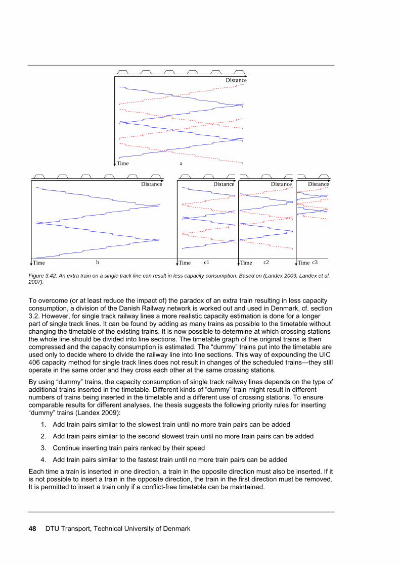
48 DTU Transport, Technical University of Denmark
a
Distance
Time
b
Distance
Time c1
Distance
Time c2
Distance
Time c3
Distance
Time Figure 3.42: An extra train on a single track line can result in less capacity consumption. Based on (Landex 2009, Landex et al. 2007).
To overcome (or at least reduce the impact of) the paradox of an extra train resulting in less capacity consumption, a division of the Danish Railway network is worked out and used in Denmark, cf. section 3.2. However, for single track railway lines a more realistic capacity estimation is done for a longer part of single track lines. It can be found by adding as many trains as possible to the timetable without changing the timetable of the existing trains. It is now possible to determine at which crossing stations the whole line should be divided into line sections. The timetable graph of the original trains is then compressed and the capacity consumption is estimated. The “dummy” trains put into the timetable are used only to decide where to divide the railway line into line sections. This way of expounding the UIC 406 capacity method for single track lines does not result in changes of the scheduled trains—they still operate in the same order and they cross each other at the same crossing stations.
By using “dummy” trains, the capacity consumption of single track railway lines depends on the type of additional trains inserted in the timetable. Different kinds of “dummy” train might result in different numbers of trains being inserted in the timetable and a different use of crossing stations. To ensure comparable results for different analyses, the thesis suggests the following priority rules for inserting “dummy” trains (Landex 2009):
1. Add train pairs similar to the slowest train until no more train pairs can be added
2. Add train pairs similar to the second slowest train until no more train pairs can be added
3. Continue inserting train pairs ranked by their speed
4. Add train pairs similar to the fastest train until no more train pairs can be added
Each time a train is inserted in one direction, a train in the opposite direction must also be inserted. If it is not possible to insert a train in the opposite direction, the train in the first direction must be removed. It is permitted to insert a train only if a conflict-free timetable can be maintained.
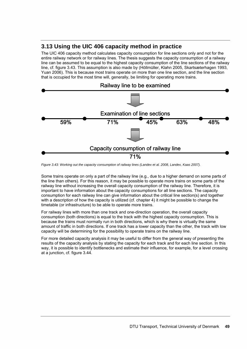
DTU Transport, Technical University of Denmark 49
3.13 Using the UIC 406 capacity method in practice The UIC 406 capacity method calculates capacity consumption for line sections only and not for the entire railway network or for railway lines. The thesis suggests the capacity consumption of a railway line can be assumed to be equal to the highest capacity consumption of the line sections of the railway line, cf. figure 3.43. This assumption is also made by (Höllmüller, Klahn 2005, Skartsæterhagen 1993, Yuan 2006). This is because most trains operate on more than one line section, and the line section that is occupied for the most time will, generally, be limiting for operating more trains.
Railway line to be examinedRailway line to be examined
59% 45%71% 63% 48%Examination of line sections
59% 45%71% 63% 48%59% 45%71% 63% 48%Examination of line sections
71%Capacity consumption of railway line
71%71%Capacity consumption of railway line
Figure 3.43: Working out the capacity consumption of railway lines (Landex et al. 2008, Landex, Kaas 2007).
Some trains operate on only a part of the railway line (e.g., due to a higher demand on some parts of the line than others). For this reason, it may be possible to operate more trains on some parts of the railway line without increasing the overall capacity consumption of the railway line. Therefore, it is important to have information about the capacity consumptions for all line sections. The capacity consumption for each railway line can give information about the critical line section(s) and together with a description of how the capacity is utilized (cf. chapter 4) it might be possible to change the timetable (or infrastructure) to be able to operate more trains.
For railway lines with more than one track and one-direction operation, the overall capacity consumption (both directions) is equal to the track with the highest capacity consumption. This is because the trains must normally run in both directions, which is why there is virtually the same amount of traffic in both directions. If one track has a lower capacity than the other, the track with low capacity will be determining for the possibility to operate trains on the railway line.
For more detailed capacity analysis it may be useful to differ from the general way of presenting the results of the capacity analysis by stating the capacity for each track and for each line section. In this way, it is possible to identify bottlenecks and estimate their influence, for example, for a level crossing at a junction, cf. figure 3.44.
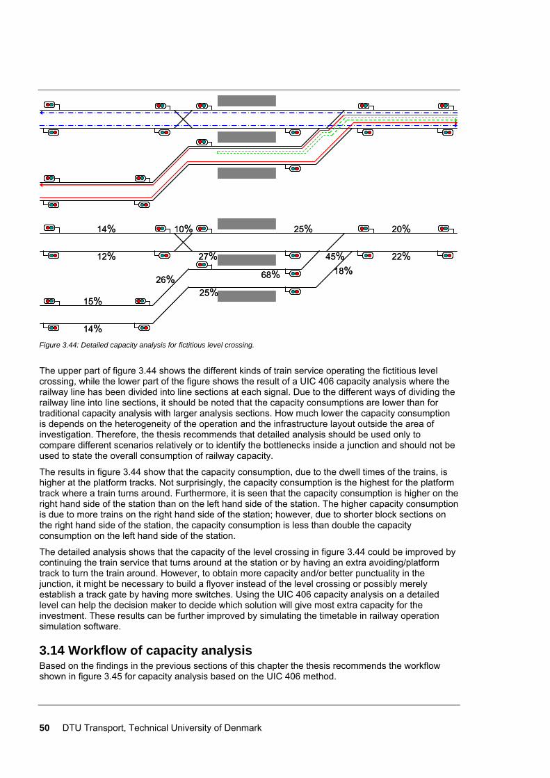
50 DTU Transport, Technical University of Denmark
20%
22%
25%14%
12% 27%
68%
25%26%
15%
14%
18%45%
10% 20%
22%
25%14%
12% 27%
68%
25%26%
15%
14%
18%45%
10%
Figure 3.44: Detailed capacity analysis for fictitious level crossing.
The upper part of figure 3.44 shows the different kinds of train service operating the fictitious level crossing, while the lower part of the figure shows the result of a UIC 406 capacity analysis where the railway line has been divided into line sections at each signal. Due to the different ways of dividing the railway line into line sections, it should be noted that the capacity consumptions are lower than for traditional capacity analysis with larger analysis sections. How much lower the capacity consumption is depends on the heterogeneity of the operation and the infrastructure layout outside the area of investigation. Therefore, the thesis recommends that detailed analysis should be used only to compare different scenarios relatively or to identify the bottlenecks inside a junction and should not be used to state the overall consumption of railway capacity.
The results in figure 3.44 show that the capacity consumption, due to the dwell times of the trains, is higher at the platform tracks. Not surprisingly, the capacity consumption is the highest for the platform track where a train turns around. Furthermore, it is seen that the capacity consumption is higher on the right hand side of the station than on the left hand side of the station. The higher capacity consumption is due to more trains on the right hand side of the station; however, due to shorter block sections on the right hand side of the station, the capacity consumption is less than double the capacity consumption on the left hand side of the station.
The detailed analysis shows that the capacity of the level crossing in figure 3.44 could be improved by continuing the train service that turns around at the station or by having an extra avoiding/platform track to turn the train around. However, to obtain more capacity and/or better punctuality in the junction, it might be necessary to build a flyover instead of the level crossing or possibly merely establish a track gate by having more switches. Using the UIC 406 capacity analysis on a detailed level can help the decision maker to decide which solution will give most extra capacity for the investment. These results can be further improved by simulating the timetable in railway operation simulation software.
3.14 Workflow of capacity analysis Based on the findings in the previous sections of this chapter the thesis recommends the workflow shown in figure 3.45 for capacity analysis based on the UIC 406 method.

DTU Transport, Technical University of Denmark 51
Build up infrastructure
Build up timetable
More than two tracks Single track
Divide into line sections
Compress the timetable graph
Double track
Divide into line sections
Work out capacity consumption for each line section
Large difference in capacity consumption for the tracks
Change track for train(s)
Compress time table graph
Add as many “dummy” trains as possible without changing the original
timetable/infrastructure
Divide into line sections at each crossing station in use
Compress the original timetable graph
Work out capacity consumption (without additional “dummy” trains) for
each line section
Work out capacity consumption for each line section
Capacity consumption of railway line equal to highest capacity consumption
of line sections
Yes No
Divide infrastructure into overall line sections at transition stations
Figure 3.45: Workflow of measuring capacity consumption of railway lines (Landex et al. 2008).
First, the infrastructure to be analysed must be built up to a detailed level in a timetabling system. Then the timetable to be analysed must be established. Based on the infrastructure, the railway lines are divided into overall line sections (at the transition stations) of single track lines, double track lines, and lines with more tracks respectively. These overall line sections are then analysed in different ways depending on the number of tracks.
Double track railway lines are the easiest to examine. In Denmark, the overall line sections are equal to the line sections whereupon the timetable graphs are compressed, according to the UIC 406 capacity method. When the timetable graphs have been compressed, the capacity consumption of the line section is worked out.
Single track railway lines are more complicated to examine as it is necessary to add as many trains as possible without changing the original timetable or infrastructure (cf. section 3.12.2). Then the overall single track line section is divided into line sections for each time a crossing station is in use. When the railway line has been divided into line sections, the timetable graphs of the original timetable are compressed according to the UIC 406 capacity method and the capacity consumption of each line section is worked out (without the extra “dummy” trains).
For overall line sections containing three, four or more tracks another approach must be used. Tracks that are used only for traffic in one direction must be divided into line sections in the same way as double track lines, while tracks used for traffic in both directions must be divided into line sections in the same way as single track lines, and the intersection of division points is then used to find the final line sections. After the division into line sections, the timetable graphs are compressed and the capacity consumption for each line section is worked out. If it appears that there is a large difference in the capacity consumption between the tracks, one or more trains must change tracks and the compression is redone until the capacity consumption of the tracks is more or less equal.
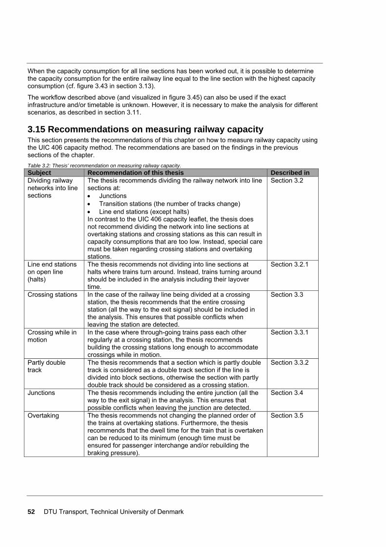
52 DTU Transport, Technical University of Denmark
When the capacity consumption for all line sections has been worked out, it is possible to determine the capacity consumption for the entire railway line equal to the line section with the highest capacity consumption (cf. figure 3.43 in section 3.13).
The workflow described above (and visualized in figure 3.45) can also be used if the exact infrastructure and/or timetable is unknown. However, it is necessary to make the analysis for different scenarios, as described in section 3.11.
3.15 Recommendations on measuring railway capacity This section presents the recommendations of this chapter on how to measure railway capacity using the UIC 406 capacity method. The recommendations are based on the findings in the previous sections of the chapter. Table 3.2: Thesis’ recommendation on measuring railway capacity. Subject Recommendation of this thesis Described in Dividing railway networks into line sections
The thesis recommends dividing the railway network into line sections at: • Junctions • Transition stations (the number of tracks change) • Line end stations (except halts) In contrast to the UIC 406 capacity leaflet, the thesis does not recommend dividing the network into line sections at overtaking stations and crossing stations as this can result in capacity consumptions that are too low. Instead, special care must be taken regarding crossing stations and overtaking stations.
Section 3.2
Line end stations on open line (halts)
The thesis recommends not dividing into line sections at halts where trains turn around. Instead, trains turning around should be included in the analysis including their layover time.
Section 3.2.1
Crossing stations In the case of the railway line being divided at a crossing station, the thesis recommends that the entire crossing station (all the way to the exit signal) should be included in the analysis. This ensures that possible conflicts when leaving the station are detected.
Section 3.3
Crossing while in motion
In the case where through-going trains pass each other regularly at a crossing station, the thesis recommends building the crossing stations long enough to accommodate crossings while in motion.
Section 3.3.1
Partly double track
The thesis recommends that a section which is partly double track is considered as a double track section if the line is divided into block sections, otherwise the section with partly double track should be considered as a crossing station.
Section 3.3.2
Junctions The thesis recommends including the entire junction (all the way to the exit signal) in the analysis. This ensures that possible conflicts when leaving the junction are detected.
Section 3.4
Overtaking The thesis recommends not changing the planned order of the trains at overtaking stations. Furthermore, the thesis recommends that the dwell time for the train that is overtaken can be reduced to its minimum (enough time must be ensured for passenger interchange and/or rebuilding the braking pressure).
Section 3.5
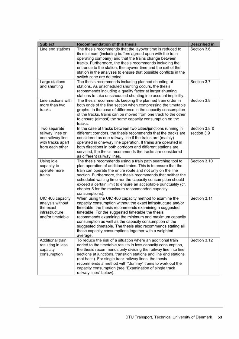
DTU Transport, Technical University of Denmark 53
Subject Recommendation of this thesis Described in Line end stations The thesis recommends that the layover time is reduced to
its minimum (including buffers agreed upon with the train operating company) and that the trains change between tracks. Furthermore, the thesis recommends including the entrance to the station, the layover time and the exit of the station in the analyses to ensure that possible conflicts in the switch zone are detected.
Section 3.6
Large stations and shunting
The thesis recommends including planned shunting at stations. As unscheduled shunting occurs, the thesis recommends including a quality factor at larger shunting stations to take unscheduled shunting into account implicitly.
Section 3.7
Line sections with more than two tracks
The thesis recommends keeping the planned train order in both ends of the line section when compressing the timetable graphs. In the case of difference in the capacity consumption of the tracks, trains can be moved from one track to the other to ensure (almost) the same capacity consumption on the tracks.
Section 3.8
Two separate railway lines or one railway line with tracks apart from each other
In the case of tracks between two cities/junctions running in different corridors, the thesis recommends that the tracks are considered as one railway line if the trains are (mainly) operated in one-way line operation. If trains are operated in both directions in both corridors and different stations are serviced, the thesis recommends the tracks are considered as different railway lines.
Section 3.8 & section 3.9
Using idle capacity to operate more trains
The thesis recommends using a train path searching tool to plan operation of additional trains. This is to ensure that the train can operate the entire route and not only on the line section. Furthermore, the thesis recommends that neither the scheduled waiting time nor the capacity consumption should exceed a certain limit to ensure an acceptable punctuality (cf. chapter 5 for the maximum recommended capacity consumptions).
Section 3.10
UIC 406 capacity analysis without the exact infrastructure and/or timetable
When using the UIC 406 capacity method to examine the capacity consumption without the exact infrastructure and/or timetable, the thesis recommends examining a suggested timetable. For the suggested timetable the thesis recommends examining the minimum and maximum capacity consumption as well as the capacity consumption of the suggested timetable. The thesis also recommends stating all these capacity consumptions together with a weighted average.
Section 3.11
Additional train resulting in less capacity consumption
To reduce the risk of a situation where an additional train added to the timetable results in less capacity consumption, the thesis recommends only dividing the railway line into line sections at junctions, transition stations and line end stations (not halts). For single track railway lines, the thesis recommends a method with “dummy” trains to work out the capacity consumption (see “Examination of single track railway lines” below).
Section 3.12
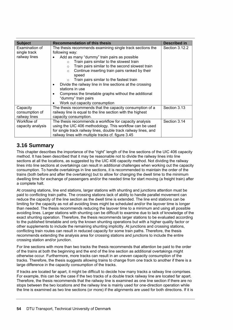
54 DTU Transport, Technical University of Denmark
Subject Recommendation of this thesis Described in Examination of single track railway lines
The thesis recommends examining single track sections the following way: • Add as many “dummy” train pairs as possible
o Train pairs similar to the slowest train o Train pairs similar to the second slowest train o Continue inserting train pairs ranked by their
speed o Train pairs similar to the fastest train
• Divide the railway line in line sections at the crossing stations in use
• Compress the timetable graphs without the additional “dummy” train pairs
• Work out capacity consumption
Section 3.12.2
Capacity consumption of railway lines
The thesis recommends that the capacity consumption of a railway line is equal to the line section with the highest capacity consumption.
Section 3.13
Workflow of capacity analysis
The thesis recommends a workflow for capacity analysis using the UIC 406 methodology. This workflow can be used for single track railway lines, double track railway lines, and railway lines with multiple tracks cf. figure 3.45
Section 3.14
3.16 Summary This chapter describes the importance of the “right” length of the line sections of the UIC 406 capacity method. It has been described that it may be reasonable not to divide the railway lines into line sections at all the locations, as suggested by the UIC 406 capacity method. Not dividing the railway lines into line sections at overtakings can result in additional challenges when working out the capacity consumption. To handle overtakings in line sections, it is recommended to maintain the order of the trains (both before and after the overtaking) but to allow for changing the dwell time to the minimum dwelling time for exchange of passengers and/or the needed time for start moving (a freight train) after a complete halt.
At crossing stations, line end stations, larger stations with shunting and junctions attention must be paid to conflicting train paths. The crossing stations lack of ability to handle parallel movement can reduce the capacity of the line section as the dwell time is extended. The line end stations can be limiting for the capacity as not all avoiding lines might be scheduled and/or the layover time is longer than needed. The thesis recommends reducing the layover time to a minimum and using all possible avoiding lines. Larger stations with shunting can be difficult to examine due to lack of knowledge of the exact shunting operation. Therefore, the thesis recommends larger stations to be evaluated according to the published timetable and only the known shunting operations but with a higher quality factor or other supplements to include the remaining shunting implicitly. At junctions and crossing stations, conflicting train routes can result in reduced capacity for some train paths. Therefore, the thesis recommends extending the analysis area for crossing stations and junctions to include the entire crossing station and/or junction.
For line sections with more than two tracks the thesis recommends that attention be paid to the order of the trains at both the beginning and the end of the line section as additional overtakings might otherwise occur. Furthermore, more tracks can result in an uneven capacity consumption of the tracks. Therefore, the thesis suggests allowing trains to change from one track to another if there is a large difference in the capacity consumption of the tracks.
If tracks are located far apart, it might be difficult to decide how many tracks a railway line comprises. For example, this can be the case if the two tracks of a double track railway line are located far apart. Therefore, the thesis recommends that the railway line is examined as one line section if there are no stops between the two locations and the railway line is mainly used for one-direction operation while the line is examined as two line sections (or more) if the alignments are used for both directions. If it is
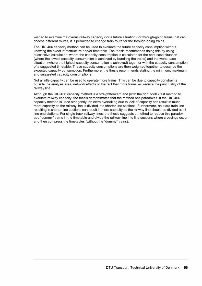
DTU Transport, Technical University of Denmark 55
wished to examine the overall railway capacity (for a future situation) for through-going trains that can choose different routes, it is permitted to change train route for the through-going trains.
The UIC 406 capacity method can be used to evaluate the future capacity consumption without knowing the exact infrastructure and/or timetable. The thesis recommends doing this by using successive calculation, where the capacity consumption is calculated for the best-case situation (where the lowest capacity consumption is achieved by bundling the trains) and the worst-case situation (where the highest capacity consumption is achieved) together with the capacity consumption of a suggested timetable. These capacity consumptions are then weighted together to describe the expected capacity consumption. Furthermore, the thesis recommends stating the minimum, maximum and suggested capacity consumptions.
Not all idle capacity can be used to operate more trains. This can be due to capacity constraints outside the analysis area, network effects or the fact that more trains will reduce the punctuality of the railway line.
Although the UIC 406 capacity method is a straightforward and (with the right tools) fast method to evaluate railway capacity, the thesis demonstrates that the method has paradoxes. If the UIC 406 capacity method is used stringently, an extra overtaking due to lack of capacity can result in much more capacity as the railway line is divided into shorter line sections. Furthermore, an extra train line resulting in shorter line sections can result in more capacity as the railway line should be divided at all line end stations. For single track railway lines, the thesis suggests a method to reduce this paradox: add “dummy” trains in the timetable and divide the railway line into line sections where crossings occur and then compress the timetables (without the “dummy” trains).

56 DTU Transport, Technical University of Denmark
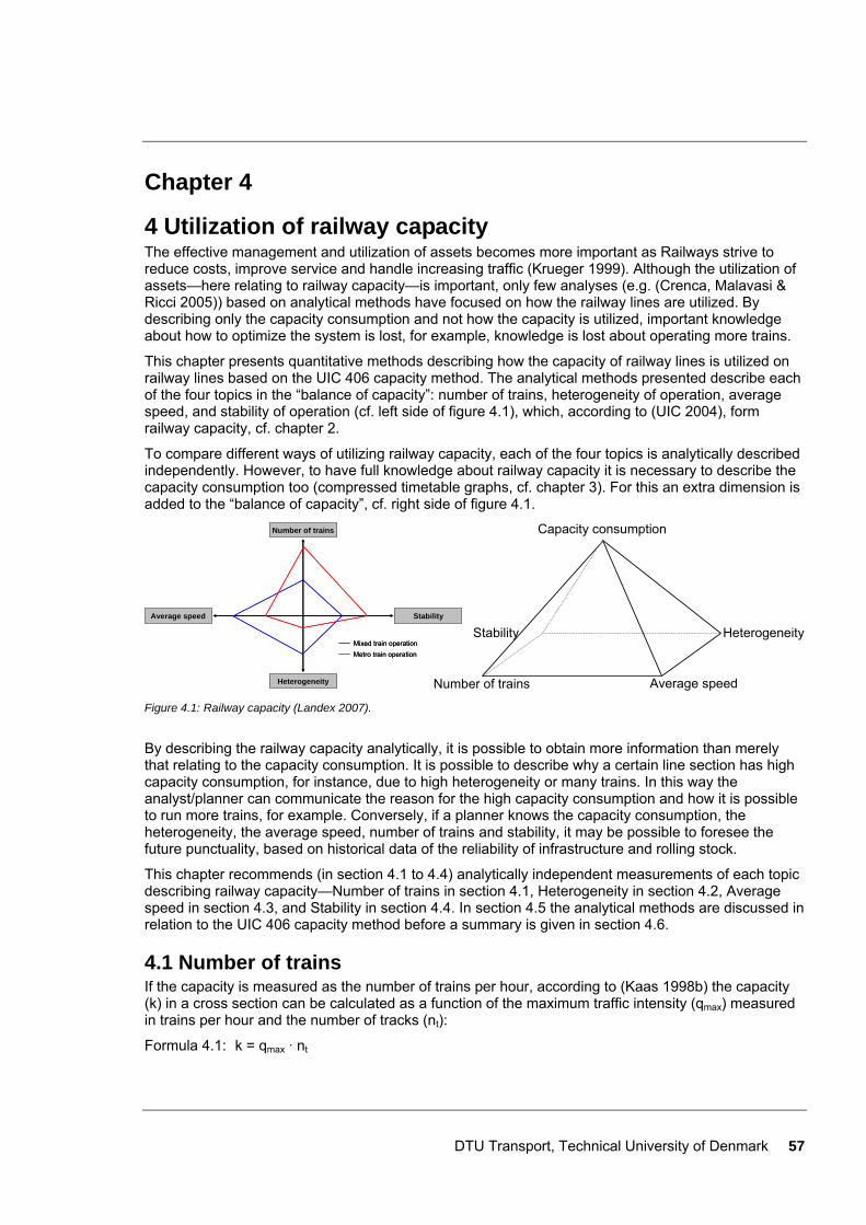
DTU Transport, Technical University of Denmark 57
Chapter 4
4 Utilization of railway capacity The effective management and utilization of assets becomes more important as Railways strive to reduce costs, improve service and handle increasing traffic (Krueger 1999). Although the utilization of assets—here relating to railway capacity—is important, only few analyses (e.g. (Crenca, Malavasi & Ricci 2005)) based on analytical methods have focused on how the railway lines are utilized. By describing only the capacity consumption and not how the capacity is utilized, important knowledge about how to optimize the system is lost, for example, knowledge is lost about operating more trains.
This chapter presents quantitative methods describing how the capacity of railway lines is utilized on railway lines based on the UIC 406 capacity method. The analytical methods presented describe each of the four topics in the “balance of capacity”: number of trains, heterogeneity of operation, average speed, and stability of operation (cf. left side of figure 4.1), which, according to (UIC 2004), form railway capacity, cf. chapter 2.
To compare different ways of utilizing railway capacity, each of the four topics is analytically described independently. However, to have full knowledge about railway capacity it is necessary to describe the capacity consumption too (compressed timetable graphs, cf. chapter 3). For this an extra dimension is added to the “balance of capacity”, cf. right side of figure 4.1.
Average speed StabilityAverage speed Stability
Heterogeneity
Number of trains
Heterogeneity
Number of trains
Mixed train operationMixed train operationMetro train operationMetro train operation
Number of trains
Stability Heterogeneity
Average speed
Capacity consumption
Figure 4.1: Railway capacity (Landex 2007).
By describing the railway capacity analytically, it is possible to obtain more information than merely that relating to the capacity consumption. It is possible to describe why a certain line section has high capacity consumption, for instance, due to high heterogeneity or many trains. In this way the analyst/planner can communicate the reason for the high capacity consumption and how it is possible to run more trains, for example. Conversely, if a planner knows the capacity consumption, the heterogeneity, the average speed, number of trains and stability, it may be possible to foresee the future punctuality, based on historical data of the reliability of infrastructure and rolling stock.
This chapter recommends (in section 4.1 to 4.4) analytically independent measurements of each topic describing railway capacity—Number of trains in section 4.1, Heterogeneity in section 4.2, Average speed in section 4.3, and Stability in section 4.4. In section 4.5 the analytical methods are discussed in relation to the UIC 406 capacity method before a summary is given in section 4.6.
4.1 Number of trains If the capacity is measured as the number of trains per hour, according to (Kaas 1998b) the capacity (k) in a cross section can be calculated as a function of the maximum traffic intensity (qmax) measured in trains per hour and the number of tracks (nt):
Formula 4.1: k = qmax · nt
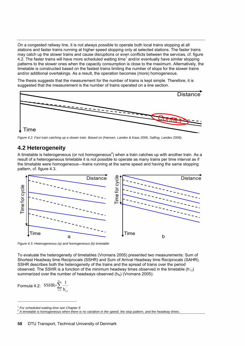
58 DTU Transport, Technical University of Denmark
On a congested railway line, it is not always possible to operate both local trains stopping at all stations and faster trains running at higher speed stopping only at selected stations. The faster trains may catch up the slower trains and cause disruptions or even conflicts between the services, cf. figure 4.2. The faster trains will have more scheduled waiting time1 and/or eventually have similar stopping patterns to the slower ones when the capacity consumption is close to the maximum. Alternatively, the timetable is constructed based on the fastest trains limiting the number of stops for the slower trains and/or additional overtakings. As a result, the operation becomes (more) homogeneous.
The thesis suggests that the measurement for the number of trains is kept simple. Therefore, it is suggested that the measurement is the number of trains operated on a line section.
Distance
Time Figure 4.2: Fast train catching up a slower train. Based on (Hansen, Landex & Kaas 2006, Salling, Landex 2006).
4.2 Heterogeneity A timetable is heterogeneous (or not homogeneous2) when a train catches up with another train. As a result of a heterogeneous timetable it is not possible to operate as many trains per time interval as if the timetable were homogeneous—trains running at the same speed and having the same stopping pattern, cf. figure 4.3.
Tim
e fo
r cyc
le
a
Tim
e fo
r cyc
le
bTime
Distance
Time
Distance
Figure 4.3: Heterogeneous (a) and homogeneous (b) timetable.
To evaluate the heterogeneity of timetables (Vromans 2005) presented two measurements: Sum of Shortest Headway time Reciprocals (SSHR) and Sum of Arrival Headway time Reciprocals (SAHR). SSHR describes both the heterogeneity of the trains and the spread of trains over the period observed. The SSHR is a function of the minimum headway times observed in the timetable (h-
t,i) summarized over the number of headways observed (hN) (Vromans 2005):
Formula 4.2: ∑=
=N
_
h
1i t,ih1SSHR
1 For scheduled waiting time see Chapter 9 2 A timetable is homogeneous when there is no variation in the speed, the stop pattern, and the headway times.
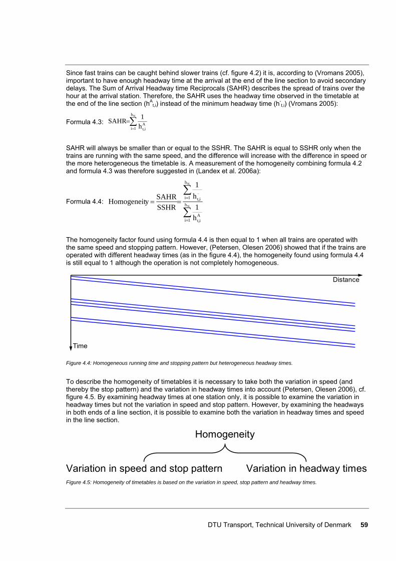
DTU Transport, Technical University of Denmark 59
Since fast trains can be caught behind slower trains (cf. figure 4.2) it is, according to (Vromans 2005), important to have enough headway time at the arrival at the end of the line section to avoid secondary delays. The Sum of Arrival Headway time Reciprocals (SAHR) describes the spread of trains over the hour at the arrival station. Therefore, the SAHR uses the headway time observed in the timetable at the end of the line section (hA
t,i) instead of the minimum headway time (h-t,i) (Vromans 2005):
Formula 4.3: ∑=
=Nh
1iAt,ih
1SAHR
SAHR will always be smaller than or equal to the SSHR. The SAHR is equal to SSHR only when the trains are running with the same speed, and the difference will increase with the difference in speed or the more heterogeneous the timetable is. A measurement of the homogeneity combining formula 4.2 and formula 4.3 was therefore suggested in (Landex et al. 2006a):
Formula 4.4:
∑
∑
=
===
N
N
_
h
1iA
it,
h
1i it,
h1
h1
SSHRSAHR y Homogeneit
The homogeneity factor found using formula 4.4 is then equal to 1 when all trains are operated with the same speed and stopping pattern. However, (Petersen, Olesen 2006) showed that if the trains are operated with different headway times (as in the figure 4.4), the homogeneity found using formula 4.4 is still equal to 1 although the operation is not completely homogeneous.
Time
Distance
Figure 4.4: Homogeneous running time and stopping pattern but heterogeneous headway times.
To describe the homogeneity of timetables it is necessary to take both the variation in speed (and thereby the stop pattern) and the variation in headway times into account (Petersen, Olesen 2006), cf. figure 4.5. By examining headway times at one station only, it is possible to examine the variation in headway times but not the variation in speed and stop pattern. However, by examining the headways in both ends of a line section, it is possible to examine both the variation in headway times and speed in the line section.
Homogeneity
Variation in speed and stop pattern Variation in headway times Figure 4.5: Homogeneity of timetables is based on the variation in speed, stop pattern and headway times.
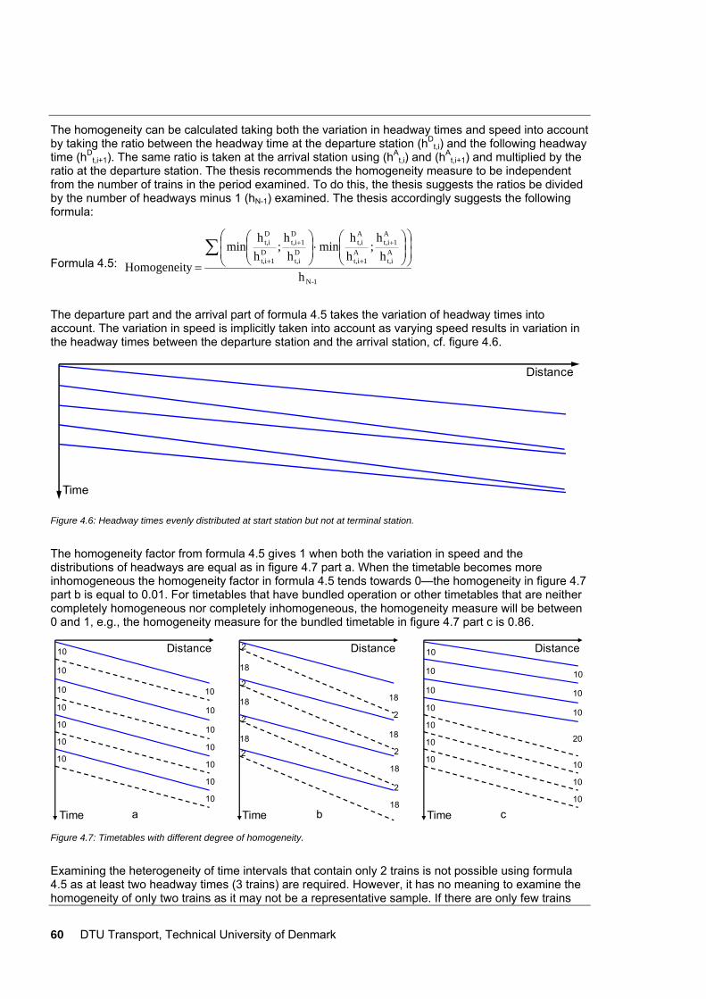
60 DTU Transport, Technical University of Denmark
The homogeneity can be calculated taking both the variation in headway times and speed into account by taking the ratio between the headway time at the departure station (hD
t,i) and the following headway time (hD
t,i+1). The same ratio is taken at the arrival station using (hAt,i) and (hA
t,i+1) and multiplied by the ratio at the departure station. The thesis recommends the homogeneity measure to be independent from the number of trains in the period examined. To do this, the thesis suggests the ratios be divided by the number of headways minus 1 (hN-1) examined. The thesis accordingly suggests the following formula:
Formula 4.5:
1-N
Ait,
A1it,
A1it,
Ait,
Dit,
D1it,
D1it,
Dit,
h
hh
;hh
min h
h;
hh
min
y Homogeneit∑ ⎟
⎟⎠
⎞⎜⎜⎝
⎛⎟⎟⎠
⎞⎜⎜⎝
⎛⋅⎟⎟⎠
⎞⎜⎜⎝
⎛
=
+
+
+
+
The departure part and the arrival part of formula 4.5 takes the variation of headway times into account. The variation in speed is implicitly taken into account as varying speed results in variation in the headway times between the departure station and the arrival station, cf. figure 4.6.
Time
Distance
Figure 4.6: Headway times evenly distributed at start station but not at terminal station.
The homogeneity factor from formula 4.5 gives 1 when both the variation in speed and the distributions of headways are equal as in figure 4.7 part a. When the timetable becomes more inhomogeneous the homogeneity factor in formula 4.5 tends towards 0—the homogeneity in figure 4.7 part b is equal to 0.01. For timetables that have bundled operation or other timetables that are neither completely homogeneous nor completely inhomogeneous, the homogeneity measure will be between 0 and 1, e.g., the homogeneity measure for the bundled timetable in figure 4.7 part c is 0.86.
b
18
18
18
18
18
18
18
2
2
2
2
2
2
2
a
10
10
10
10
10
10
10
10
10
10
10
10
10
10
c
10
10
10
10
10
10
10
10
10
10
20
10
10
10
Time
Distance DistanceDistance
TimeTime Figure 4.7: Timetables with different degree of homogeneity.
Examining the heterogeneity of time intervals that contain only 2 trains is not possible using formula 4.5 as at least two headway times (3 trains) are required. However, it has no meaning to examine the homogeneity of only two trains as it may not be a representative sample. If there are only few trains
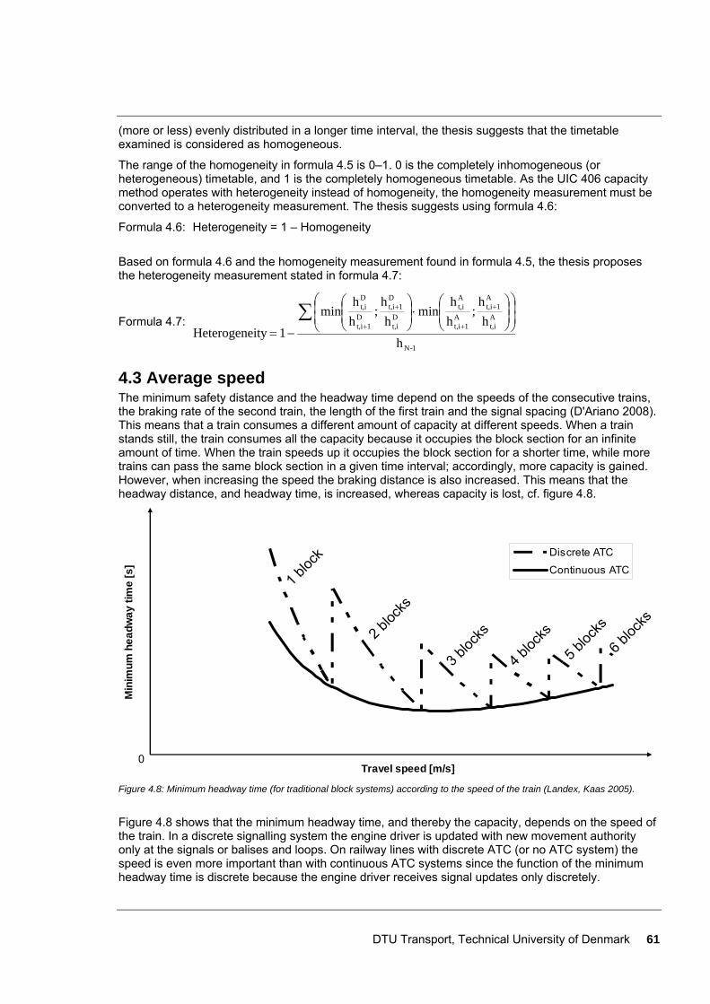
DTU Transport, Technical University of Denmark 61
(more or less) evenly distributed in a longer time interval, the thesis suggests that the timetable examined is considered as homogeneous.
The range of the homogeneity in formula 4.5 is 0–1. 0 is the completely inhomogeneous (or heterogeneous) timetable, and 1 is the completely homogeneous timetable. As the UIC 406 capacity method operates with heterogeneity instead of homogeneity, the homogeneity measurement must be converted to a heterogeneity measurement. The thesis suggests using formula 4.6:
Formula 4.6: Heterogeneity = 1 – Homogeneity
Based on formula 4.6 and the homogeneity measurement found in formula 4.5, the thesis proposes the heterogeneity measurement stated in formula 4.7:
Formula 4.7:
1-N
At,i
A1t,i
A1t,i
At,i
Dt,i
D1t,i
D1t,i
Dt,i
h
hh
;hh
min h
h;
hh
min
1ity Heterogene∑ ⎟
⎟⎠
⎞⎜⎜⎝
⎛⎟⎟⎠
⎞⎜⎜⎝
⎛⋅⎟⎟⎠
⎞⎜⎜⎝
⎛
−=
+
+
+
+
4.3 Average speed The minimum safety distance and the headway time depend on the speeds of the consecutive trains, the braking rate of the second train, the length of the first train and the signal spacing (D'Ariano 2008). This means that a train consumes a different amount of capacity at different speeds. When a train stands still, the train consumes all the capacity because it occupies the block section for an infinite amount of time. When the train speeds up it occupies the block section for a shorter time, while more trains can pass the same block section in a given time interval; accordingly, more capacity is gained. However, when increasing the speed the braking distance is also increased. This means that the headway distance, and headway time, is increased, whereas capacity is lost, cf. figure 4.8.
Travel speed [m/s]
Min
imum
hea
dway
tim
e [s
]
Discrete ATC
Continuous ATC1 b
lock
2 bloc
ks
3 bloc
ks
4 bloc
ks
5 bloc
ks
6 bloc
ks
0
Figure 4.8: Minimum headway time (for traditional block systems) according to the speed of the train (Landex, Kaas 2005).
Figure 4.8 shows that the minimum headway time, and thereby the capacity, depends on the speed of the train. In a discrete signalling system the engine driver is updated with new movement authority only at the signals or balises and loops. On railway lines with discrete ATC (or no ATC system) the speed is even more important than with continuous ATC systems since the function of the minimum headway time is discrete because the engine driver receives signal updates only discretely.
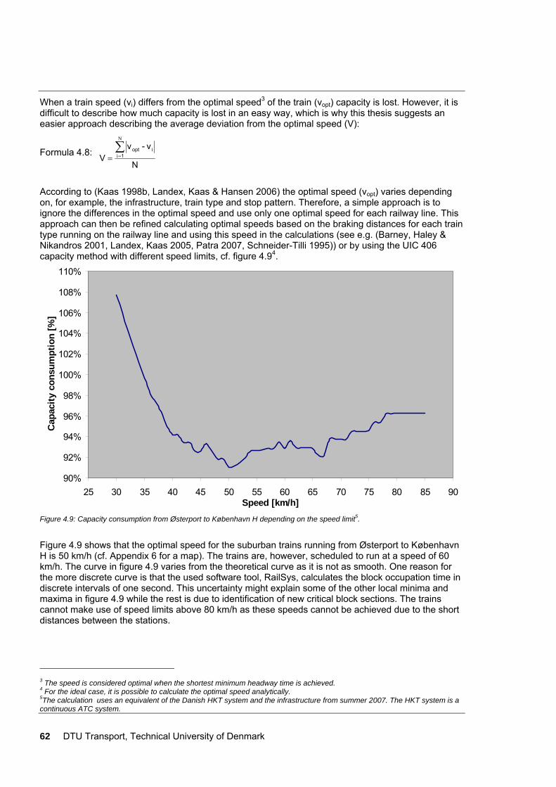
62 DTU Transport, Technical University of Denmark
When a train speed (vi) differs from the optimal speed3 of the train (vopt) capacity is lost. However, it is difficult to describe how much capacity is lost in an easy way, which is why this thesis suggests an easier approach describing the average deviation from the optimal speed (V):
Formula 4.8: N
v-v V 1
iopt∑==
N
i
According to (Kaas 1998b, Landex, Kaas & Hansen 2006) the optimal speed (vopt) varies depending on, for example, the infrastructure, train type and stop pattern. Therefore, a simple approach is to ignore the differences in the optimal speed and use only one optimal speed for each railway line. This approach can then be refined calculating optimal speeds based on the braking distances for each train type running on the railway line and using this speed in the calculations (see e.g. (Barney, Haley & Nikandros 2001, Landex, Kaas 2005, Patra 2007, Schneider-Tilli 1995)) or by using the UIC 406 capacity method with different speed limits, cf. figure 4.94.
90%
92%
94%
96%
98%
100%
102%
104%
106%
108%
110%
25 30 35 40 45 50 55 60 65 70 75 80 85 90Speed [km/h]
Cap
acity
con
sum
ptio
n [%
]
Figure 4.9: Capacity consumption from Østerport to København H depending on the speed limit5.
Figure 4.9 shows that the optimal speed for the suburban trains running from Østerport to København H is 50 km/h (cf. Appendix 6 for a map). The trains are, however, scheduled to run at a speed of 60 km/h. The curve in figure 4.9 varies from the theoretical curve as it is not as smooth. One reason for the more discrete curve is that the used software tool, RailSys, calculates the block occupation time in discrete intervals of one second. This uncertainty might explain some of the other local minima and maxima in figure 4.9 while the rest is due to identification of new critical block sections. The trains cannot make use of speed limits above 80 km/h as these speeds cannot be achieved due to the short distances between the stations.
3 The speed is considered optimal when the shortest minimum headway time is achieved. 4 For the ideal case, it is possible to calculate the optimal speed analytically. 5The calculation uses an equivalent of the Danish HKT system and the infrastructure from summer 2007. The HKT system is a continuous ATC system.
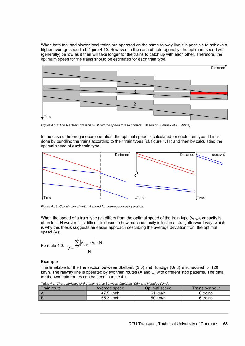
DTU Transport, Technical University of Denmark 63
When both fast and slower local trains are operated on the same railway line it is possible to achieve a higher average speed, cf. figure 4.10. However, in the case of heterogeneity, the optimum speed will (generally) be low as it then will take longer for the trains to catch up with each other. Therefore, the optimum speed for the trains should be estimated for each train type.
Distance
Time
1
3
2
Figure 4.10: The fast train (train 3) must reduce speed due to conflicts. Based on (Landex et al. 2006a).
In the case of heterogeneous operation, the optimal speed is calculated for each train type. This is done by bundling the trains according to their train types (cf. figure 4.11) and then by calculating the optimal speed of each train type.
Time
Distance
Time
Distance
Time
Distance
Figure 4.11: Calculation of optimal speed for heterogeneous operation.
When the speed of a train type (vt) differs from the optimal speed of the train type (vt,opt), capacity is often lost. However, it is difficult to describe how much capacity is lost in a straightforward way, which is why this thesis suggests an easier approach describing the average deviation from the optimal speed (V):
Formula 4.9: N
v-v V 1
toptt,∑=
⋅=
T
ttN
Example The timetable for the line section between Skelbæk (Slb) and Hundige (Und) is scheduled for 120 km/h. The railway line is operated by two train routes (A and E) with different stop patterns. The data for the two train routes can be seen in table 4.1. Table 4.1: Characteristics of the train routes between Skelbæk (Slb) and Hundige (Und). Train route Average speed Optimal speed Trains per hour A 47.5 km/h 61 km/h 6 trains E 65.3 km/h 50 km/h 6 trains
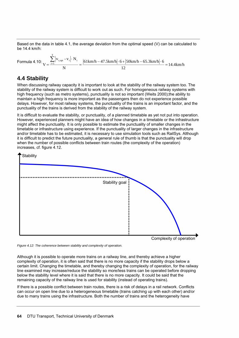
64 DTU Transport, Technical University of Denmark
Based on the data in table 4.1, the average deviation from the optimal speed (V) can be calculated to be 14.4 km/h:
Formula 4.10: km/h4.14
12665.3km/h50km/h647.5km/h61km/h
N
Nv-v V
T
1tttoptt,
=⋅−+⋅−
=⋅
=∑=
4.4 Stability When discussing railway capacity it is important to look at the stability of the railway system too. The stability of the railway system is difficult to work out as such. For homogeneous railway systems with high frequency (such as metro systems), punctuality is not so important (Weits 2000);the ability to maintain a high frequency is more important as the passengers then do not experience possible delays. However, for most railway systems, the punctuality of the trains is an important factor, and the punctuality of the trains is derived from the stability of the railway system.
It is difficult to evaluate the stability, or punctuality, of a planned timetable as yet not put into operation. However, experienced planners might have an idea of how changes in a timetable or the infrastructure might affect the punctuality. It is only possible to estimate the punctuality of smaller changes in the timetable or infrastructure using experience. If the punctuality of larger changes in the infrastructure and/or timetable has to be estimated, it is necessary to use simulation tools such as RailSys. Although it is difficult to predict the future punctuality, a general rule of thumb is that the punctuality will drop when the number of possible conflicts between train routes (the complexity of the operation) increases, cf. figure 4.12.
Complexity of operation
Stability
Stability goal
Figure 4.12: The coherence between stability and complexity of operation.
Although it is possible to operate more trains on a railway line, and thereby achieve a higher complexity of operation, it is often said that there is no more capacity if the stability drops below a certain limit. Changing the timetable, and thereby changing the complexity of operation, for the railway line examined may increase/reduce the stability so more/less trains can be operated before dropping below the stability level where it is said that there is no more capacity. It could be said that the remaining capacity of the railway line is used for stability (instead of operating trains).
If there is a possible conflict between train routes, there is a risk of delays in a rail network. Conflicts can occur on open line due to a heterogeneous timetable (trains catching up with each other) and/or due to many trains using the infrastructure. Both the number of trains and the heterogeneity have

DTU Transport, Technical University of Denmark 65
been dealt with in section 4.1 and 4.2, which is why it would be double counting to use these two measurements again for the stability measurement.
Conflicts between train routes are most often observed at stations or junctions rather than on the open line. Since the headway conflicts on the open line are dealt with in the heterogeneity measurement, only conflicts at stations are examined. The complexity of the operation at stations describes the risk of conflicts, but it is often difficult to describe despite it being easy to see that the layout of, for example, a line-end station can result in a different number of possible conflicts. An example can be seen in figure 4.13 where it is obvious that station A has more possible conflicts than station B and thereby most often will have lower stability; nevertheless, it is difficult to predict the resulting stability.
A B Figure 4.13: Different kinds of principle track layout at line-end stations.
4.4.1 Complexity of stations based on track layout
Aa,cb,d
c,d
a
b
a,cb,d
c,d
a
b
Ba,c
b,dc,d
a
b
a,c
b,dc,d
a
b
a,c
b,dc,d
a
b
Figure 4.14: Train routes (a-d) at two different kinds of line-end station.
The simplest way of calculating the conflict rates is to examine only the possible conflicts between (main) train routes. Figure 4.14 shows different train routes at station A and B. The main train routes can result in conflicts with other main train routes, cf. table 4.2. Table 4.2: Train route conflicts at station A and B.
Station A Station B 1st route 2nd route a b c d
1st route2nd route a b c d
a O – D – a O – D – b – O X C b – O – C c D X O X c D – O X d – C X O d – C X O
The letters in table 4.2 explain why the routes cannot be set at the same time, where the following abbreviations are used:
– No conflict between the 2 routes O Overlapping routes D Diverging of the 2 routes (normally not a capacity problem6) C Converging of the 2 routes X Crossing of the 2 routes which results in a conflict Hatched Train routes which cannot be set after each other
Station A contains 12 combination possibilities, where 2 train routes cannot be set at the same time. The layout of station B only contains 10 combination possibilities, where 2 train routes cannot be set at the same time. Two routes cannot be set at the same time when there are overlapping routes,
6 Diverging of routes might be a capacity problem if there are capacity problems on the diverging railway lines (e.g. due to long block sections).
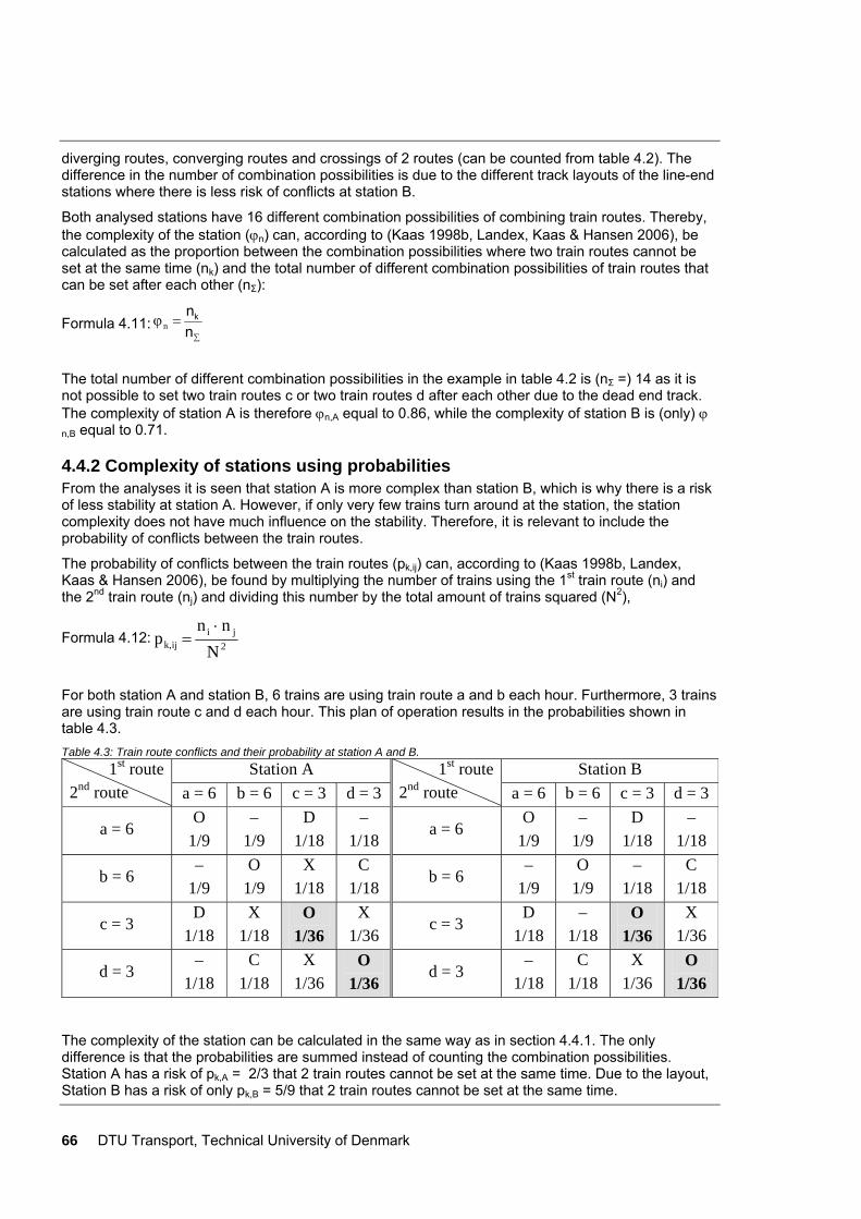
66 DTU Transport, Technical University of Denmark
diverging routes, converging routes and crossings of 2 routes (can be counted from table 4.2). The difference in the number of combination possibilities is due to the different track layouts of the line-end stations where there is less risk of conflicts at station B.
Both analysed stations have 16 different combination possibilities of combining train routes. Thereby, the complexity of the station (ϕn) can, according to (Kaas 1998b, Landex, Kaas & Hansen 2006), be calculated as the proportion between the combination possibilities where two train routes cannot be set at the same time (nk) and the total number of different combination possibilities of train routes that can be set after each other (nΣ):
Formula 4.11: ∑
=ϕnn k
n
The total number of different combination possibilities in the example in table 4.2 is (nΣ =) 14 as it is not possible to set two train routes c or two train routes d after each other due to the dead end track. The complexity of station A is therefore ϕn,A equal to 0.86, while the complexity of station B is (only) ϕ
n,B equal to 0.71.
4.4.2 Complexity of stations using probabilities From the analyses it is seen that station A is more complex than station B, which is why there is a risk of less stability at station A. However, if only very few trains turn around at the station, the station complexity does not have much influence on the stability. Therefore, it is relevant to include the probability of conflicts between the train routes.
The probability of conflicts between the train routes (pk,ij) can, according to (Kaas 1998b, Landex, Kaas & Hansen 2006), be found by multiplying the number of trains using the 1st train route (ni) and the 2nd train route (nj) and dividing this number by the total amount of trains squared (N2),
Formula 4.12: 2
jiijk, N
n n p
⋅=
For both station A and station B, 6 trains are using train route a and b each hour. Furthermore, 3 trains are using train route c and d each hour. This plan of operation results in the probabilities shown in table 4.3. Table 4.3: Train route conflicts and their probability at station A and B.
Station A Station B 1st route 2nd route a = 6 b = 6 c = 3 d = 3
1st route2nd route a = 6 b = 6 c = 3 d = 3
a = 6 O
1/9 –
1/9 D
1/18 –
1/18 a = 6
O 1/9
– 1/9
D 1/18
– 1/18
b = 6 –
1/9 O
1/9 X
1/18 C
1/18 b = 6
– 1/9
O 1/9
– 1/18
C 1/18
c = 3 D
1/18 X
1/18 O
1/36 X
1/36 c = 3
D 1/18
– 1/18
O 1/36
X 1/36
d = 3 –
1/18 C
1/18 X
1/36 O
1/36 d = 3
– 1/18
C 1/18
X 1/36
O 1/36
The complexity of the station can be calculated in the same way as in section 4.4.1. The only difference is that the probabilities are summed instead of counting the combination possibilities. Station A has a risk of pk,A = 2/3 that 2 train routes cannot be set at the same time. Due to the layout, Station B has a risk of only pk,B = 5/9 that 2 train routes cannot be set at the same time.

DTU Transport, Technical University of Denmark 67
Both analysed stations have a pΣ equal to 17/18 (where pΣ normally is equal to 1), which indicates that not all train routes can be set after one of the other train routes. This is due to the fact that it is not possible to set two train routes of c or d just after each other because of the dead end track; a train route c has to be followed by a train route d before a new train route c can be set and vice versa. Thereby the complexity of the station can be calculated as (Kaas 1998b, Landex, Kaas & Hansen 2006),
Formula 4.13: ∑
=ϕpp k
p
The complexity of station A is ϕp,A equal to 0.71, while the complexity of station B is (only) ϕp,B equal to 0.59.
The complexity of station A and station B is (in this case) lower using the probabilities of conflicts instead of using merely the train routes. The difference is because only one third of the trains are turned around at the line-end stations, for example, if two thirds of the trains had been turned around, the complexity would have been higher than using the train route complexity.
Calculation of station complexity is improved by using the probabilities of conflicting train routes. However, the probabilities would not change if the number of trains on all train routes were doubled, although the complexity of the station, and thereby the complexity of the operation, would increase in real life. The complexity of the stations is not affected by changes in the block occupation times.
4.4.3 Complexity of operation at stations using minimum headway times When using minimum headway times to evaluate the complexity of a station it is possible to evaluate the operation at the station. In this way it is possible to evaluate changes in both the infrastructure and the number of trains.
The minimum headway times for the different route combinations (th,min,ij) at station A and station B can be seen in table 4.4. The minimum headway times for two train routes c running just after each other (th,min,cc) cannot be set because the line-end track must be cleared first by a train following train route d. Likewise, it is not possible to run two train routes d immediately after each other (th,min,dd) as only one train can be on the line-end track at the same time. Table 4.4: Minimum headway times (in seconds) between train routes at station A and B.
Station A Station B 1st route 2nd route a b c d
1st route2nd route a b c d
a 105 0 157 0 a 105 0 157 0 b 0 110 114 119 b 0 110 0 119 c 110 114 44 c 110 0 44 d 0 113 360 d 0 113 360
When the headway times and the number of trains running on each train route (and thereby pk,ij) are known it is possible to calculate the occupation time for each train route (fm,ij),
Formula 4.14: ijmin,h,ijk,
ijm, t p
f ⋅ϕ
=p
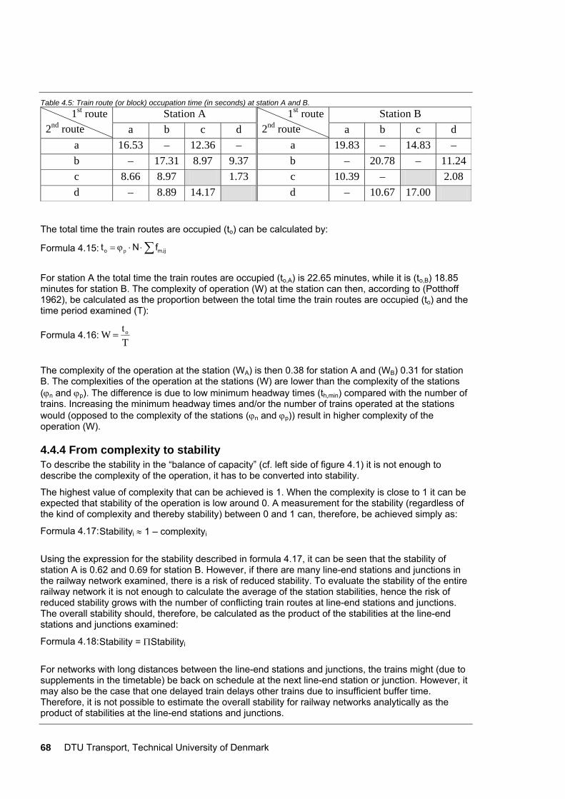
68 DTU Transport, Technical University of Denmark
Table 4.5: Train route (or block) occupation time (in seconds) at station A and B. Station A Station B 1st route
2nd route a b c d 1st route
2nd route a b c d a 16.53 – 12.36 – a 19.83 – 14.83 – b – 17.31 8.97 9.37 b – 20.78 – 11.24 c 8.66 8.97 1.73 c 10.39 – 2.08 d – 8.89 14.17 d – 10.67 17.00
The total time the train routes are occupied (to) can be calculated by:
Formula 4.15: ∑⋅⋅ϕ= ijm,o f N t p
For station A the total time the train routes are occupied (to,A) is 22.65 minutes, while it is (to,B) 18.85 minutes for station B. The complexity of operation (W) at the station can then, according to (Potthoff 1962), be calculated as the proportion between the total time the train routes are occupied (to) and the time period examined (T):
Formula 4.16: Tt W o=
The complexity of the operation at the station (WA) is then 0.38 for station A and (WB) 0.31 for station B. The complexities of the operation at the stations (W) are lower than the complexity of the stations (ϕn and ϕp). The difference is due to low minimum headway times (th,min) compared with the number of trains. Increasing the minimum headway times and/or the number of trains operated at the stations would (opposed to the complexity of the stations (ϕn and ϕp)) result in higher complexity of the operation (W).
4.4.4 From complexity to stability To describe the stability in the “balance of capacity” (cf. left side of figure 4.1) it is not enough to describe the complexity of the operation, it has to be converted into stability.
The highest value of complexity that can be achieved is 1. When the complexity is close to 1 it can be expected that stability of the operation is low around 0. A measurement for the stability (regardless of the kind of complexity and thereby stability) between 0 and 1 can, therefore, be achieved simply as:
Formula 4.17: Stabilityi ≈ 1 – complexityi
Using the expression for the stability described in formula 4.17, it can be seen that the stability of station A is 0.62 and 0.69 for station B. However, if there are many line-end stations and junctions in the railway network examined, there is a risk of reduced stability. To evaluate the stability of the entire railway network it is not enough to calculate the average of the station stabilities, hence the risk of reduced stability grows with the number of conflicting train routes at line-end stations and junctions. The overall stability should, therefore, be calculated as the product of the stabilities at the line-end stations and junctions examined:
Formula 4.18: Stability = ΠStabilityi
For networks with long distances between the line-end stations and junctions, the trains might (due to supplements in the timetable) be back on schedule at the next line-end station or junction. However, it may also be the case that one delayed train delays other trains due to insufficient buffer time. Therefore, it is not possible to estimate the overall stability for railway networks analytically as the product of stabilities at the line-end stations and junctions.
DTU Transport, Technical University of Denmark 69
For capacity analysis using the UIC 406 capacity method, the general rule is that the infrastructure should be divided into line sections at each junction, crossing station, transition station, line-end station and overtaking station (UIC 2004). This division into line sections results in short infrastructure sections for capacity analysis. As there will never be more than two stations with conflicting train routes, the product of stabilities is a good measurement for the overall stability of the line section if the UIC 406 method is followed strictly. However, in Denmark the railway lines are not always divided at the overtaking stations (cf. chapter 3). In these cases, the stability should be calculated for the overtaking station too, and this stability should be included in the product when calculating the overall stability as described in formula 4.18.
The aforementioned recommended stability measure describes only the stability of the infrastructure and not that of the operation. This is because the stability of the operation (in addition to the infrastructure) depends on the exact timetable, the rolling stock roster, and the crew schedule. Thereby, the stability of the operation depends, for example, on (UIC 1996):
• Setting of realistic departure times, making allowances for conditions of access to the station or the loading of goods
• Incorporation of greater recovery margins
• Extended stopping times at major stations
• Extended layover times for vehicles and staff
• Setting of realistic connection times between trains
Although the recommended stability measurement describes “only” the stability of the infrastructure, it is an important parameter describing the stability of the operation. This is because the stability of the operation for any timetable depends on the stability of the infrastructure.
4.5 Discussion Using the analytical description of the railway capacity it is possible to use different approaches depending on the level of detail available. For examining the stability, or complexity of stations, it is e.g. possible to use 3 different approaches. When evaluating the complexity of the infrastructure, not knowing the number of trains can give an idea of how many trains a certain station can handle. When knowing the plan of operation of the line, the approach gives more detailed information about the complexity of the station. When having more information about the infrastructure (block occupation times), the results of the analysis are the most accurate.
Due to the different analysis approaches for different levels of detail it is possible to use the analytical description of railway capacity through most planning phases. It is possible to start with simple approaches when there is only limited information and then refine the methods and results as more information becomes available.
For the heterogeneity of the operation and average speed measurement it is also possible to use different levels of detail. For the heterogeneity of the operation, the planned headway times can be used as described in section 4.2, but it is also possible to include knowledge about the infrastructure and use the buffer times instead. For the speed measurement it is possible to use the overall optimal speed or use the optimal speed for each train when calculating the deviation from the optimal speed.
The better knowledge about railway capacity achieved by the analytical methods described in this chapter can be combined with empiric data about the actually performed punctuality. In this way a large amount of knowledge is collected, which can be used as a basis to guesstimate the future punctuality of different capacity usages. This knowledge can then be used in the planning process of new timetables to predict the resulting punctuality and thereby make better timetables. The resulting punctuality of the trains can even be the basis of calculating the delays of the passengers (Nielsen, Landex & Frederiksen 2008) and in this way be an input for planning better timetables.
When it is possible to describe both the capacity consumption and how the capacity is utilized in a standardized way according to an internationally accepted standard such as the UIC 406 leaflet, it is
70 DTU Transport, Technical University of Denmark
easier to communicate railway capacity from one organization to another. The need for a straightforward way to communicate railway capacity is more relevant now than ever as the government monopoly on railway operation is fading and new operators have appeared together with increased cross-border traffic. The new organization of railways in Europe results in a greater need for communication of railway capacity between operators, infrastructure managers and authorities. The analytical description of railway capacity presented in this chapter can become part of making the future communication about railway capacity easier.
4.6 Summary Quantitative methods to describe how railway capacity is utilized based on the definition of railway capacity from the International Union of Railway (UIC), the so called UIC 406 capacity leaflet, have been developed. The methods to describe how the capacity is utilized are based on the “balance of capacity” from the UIC 406 leaflet and have a measurement for each of the four topics (Number of trains, Average speed, Heterogeneity and Stability). The four topics are normally correlated, but the measurements described in the chapter deal with each of the topics individually.
The four measurements describing the balance of capacity can be used at different levels of detail. The different levels of detail result in the possibility to describe how the capacity is expected to be utilized in all stages of planning. In the first stages of planning with only limited knowledge about infrastructure and timetable, the measurements describing how the capacity will be utilized are uncertain, but as more detailed information becomes available, a more precise description of the capacity utilization can be given.
The developed methods to describe railway capacity make it easier to communicate railway capacity between different railway agencies. This is due to the possibility of both describing the capacity consumption and how the capacity is utilized.
Although the methods developed in this chapter are a step forward in describing railway capacity, it is still not possible to describe the railway capacity of an entire railway network but “only” line sections according to the rules of the UIC 406 capacity method. In the future, the analytical description of the railway capacity presented in this chapter can be extended to deal with larger parts of the railway network—or maybe even the entire network.
Using the results from describing the railway capacity based on the method presented in this chapter, it might, in the future, be possible to develop empiric expressions for railway capacity which describe the utilization of railway capacity even more precisely. Alternatively, it might be possible to develop methods describing railway capacity based on less information so that it will be easier and require fewer data to describe railway capacity.
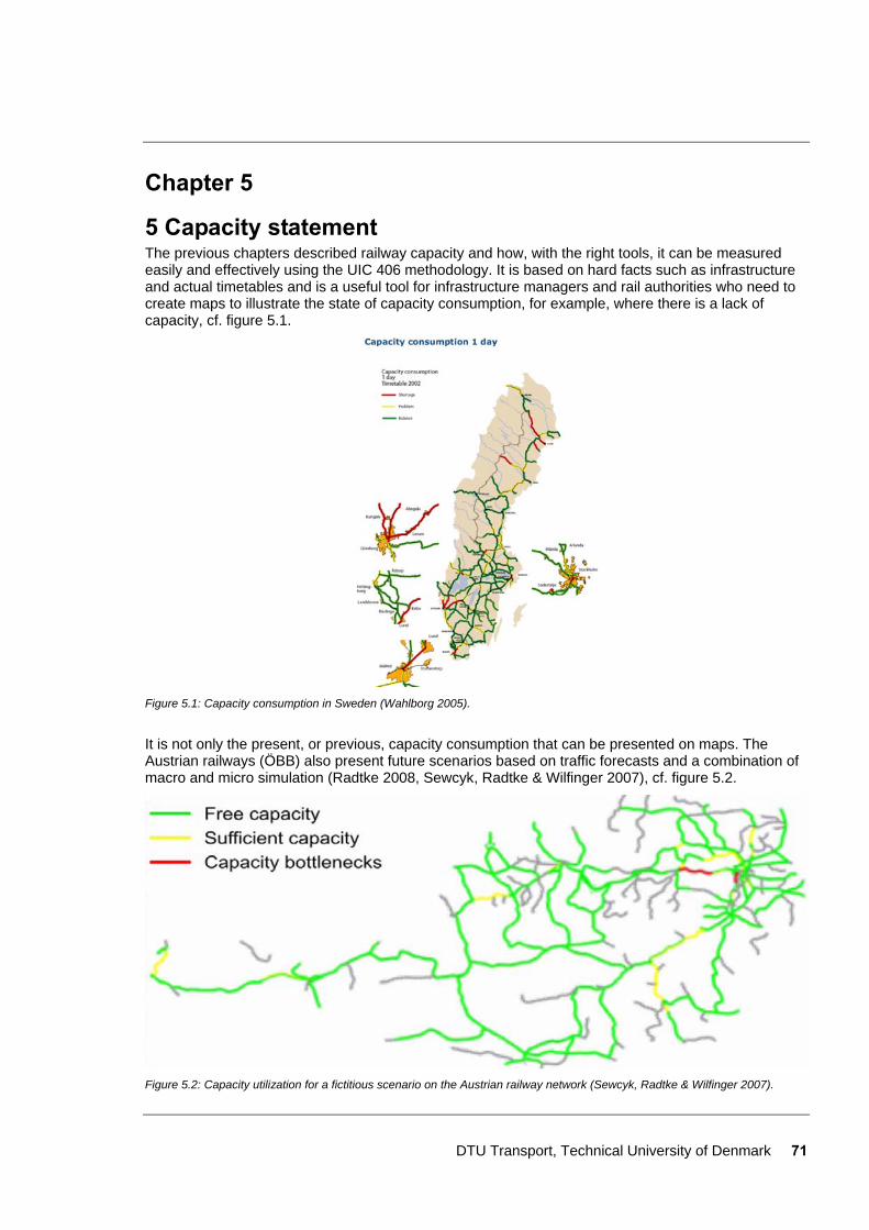
DTU Transport, Technical University of Denmark 71
Chapter 5
5 Capacity statement The previous chapters described railway capacity and how, with the right tools, it can be measured easily and effectively using the UIC 406 methodology. It is based on hard facts such as infrastructure and actual timetables and is a useful tool for infrastructure managers and rail authorities who need to create maps to illustrate the state of capacity consumption, for example, where there is a lack of capacity, cf. figure 5.1.
Figure 5.1: Capacity consumption in Sweden (Wahlborg 2005).
It is not only the present, or previous, capacity consumption that can be presented on maps. The Austrian railways (ÖBB) also present future scenarios based on traffic forecasts and a combination of macro and micro simulation (Radtke 2008, Sewcyk, Radtke & Wilfinger 2007), cf. figure 5.2.
Figure 5.2: Capacity utilization for a fictitious scenario on the Austrian railway network (Sewcyk, Radtke & Wilfinger 2007).
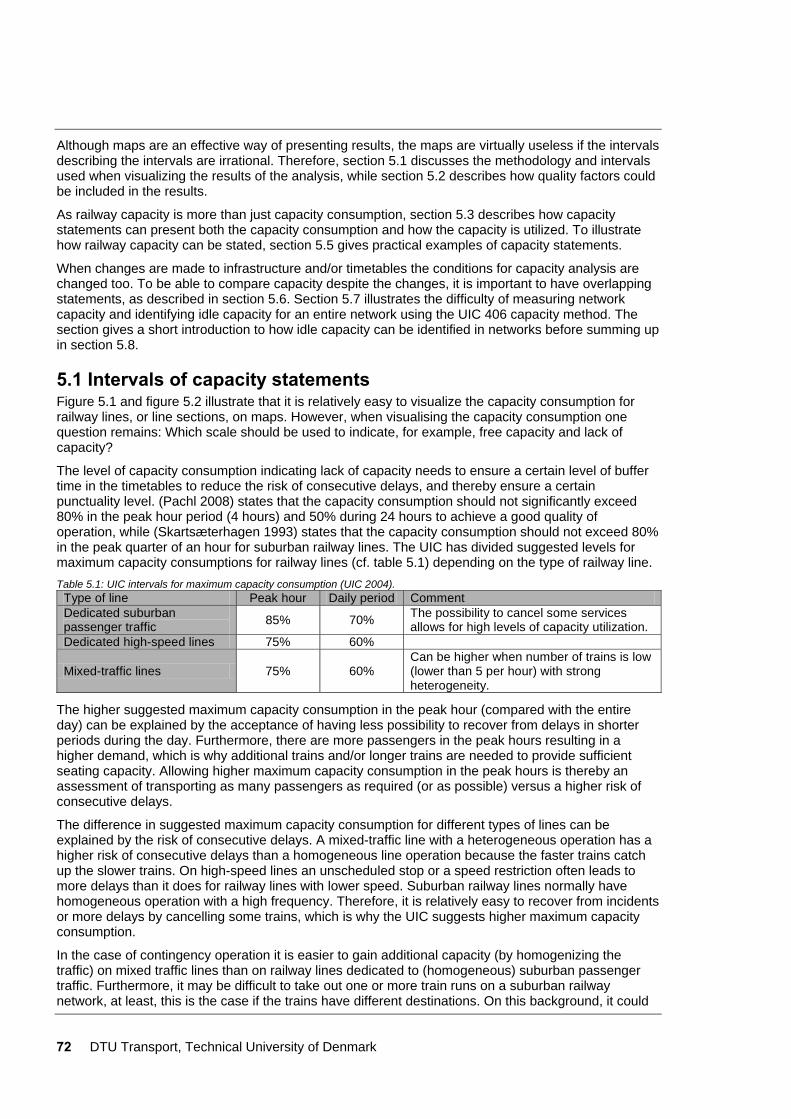
72 DTU Transport, Technical University of Denmark
Although maps are an effective way of presenting results, the maps are virtually useless if the intervals describing the intervals are irrational. Therefore, section 5.1 discusses the methodology and intervals used when visualizing the results of the analysis, while section 5.2 describes how quality factors could be included in the results.
As railway capacity is more than just capacity consumption, section 5.3 describes how capacity statements can present both the capacity consumption and how the capacity is utilized. To illustrate how railway capacity can be stated, section 5.5 gives practical examples of capacity statements.
When changes are made to infrastructure and/or timetables the conditions for capacity analysis are changed too. To be able to compare capacity despite the changes, it is important to have overlapping statements, as described in section 5.6. Section 5.7 illustrates the difficulty of measuring network capacity and identifying idle capacity for an entire network using the UIC 406 capacity method. The section gives a short introduction to how idle capacity can be identified in networks before summing up in section 5.8.
5.1 Intervals of capacity statements Figure 5.1 and figure 5.2 illustrate that it is relatively easy to visualize the capacity consumption for railway lines, or line sections, on maps. However, when visualising the capacity consumption one question remains: Which scale should be used to indicate, for example, free capacity and lack of capacity?
The level of capacity consumption indicating lack of capacity needs to ensure a certain level of buffer time in the timetables to reduce the risk of consecutive delays, and thereby ensure a certain punctuality level. (Pachl 2008) states that the capacity consumption should not significantly exceed 80% in the peak hour period (4 hours) and 50% during 24 hours to achieve a good quality of operation, while (Skartsæterhagen 1993) states that the capacity consumption should not exceed 80% in the peak quarter of an hour for suburban railway lines. The UIC has divided suggested levels for maximum capacity consumptions for railway lines (cf. table 5.1) depending on the type of railway line. Table 5.1: UIC intervals for maximum capacity consumption (UIC 2004).
Type of line Peak hour Daily period Comment Dedicated suburban passenger traffic 85% 70% The possibility to cancel some services
allows for high levels of capacity utilization. Dedicated high-speed lines 75% 60%
Mixed-traffic lines 75% 60% Can be higher when number of trains is low (lower than 5 per hour) with strong heterogeneity.
The higher suggested maximum capacity consumption in the peak hour (compared with the entire day) can be explained by the acceptance of having less possibility to recover from delays in shorter periods during the day. Furthermore, there are more passengers in the peak hours resulting in a higher demand, which is why additional trains and/or longer trains are needed to provide sufficient seating capacity. Allowing higher maximum capacity consumption in the peak hours is thereby an assessment of transporting as many passengers as required (or as possible) versus a higher risk of consecutive delays.
The difference in suggested maximum capacity consumption for different types of lines can be explained by the risk of consecutive delays. A mixed-traffic line with a heterogeneous operation has a higher risk of consecutive delays than a homogeneous line operation because the faster trains catch up the slower trains. On high-speed lines an unscheduled stop or a speed restriction often leads to more delays than it does for railway lines with lower speed. Suburban railway lines normally have homogeneous operation with a high frequency. Therefore, it is relatively easy to recover from incidents or more delays by cancelling some trains, which is why the UIC suggests higher maximum capacity consumption.
In the case of contingency operation it is easier to gain additional capacity (by homogenizing the traffic) on mixed traffic lines than on railway lines dedicated to (homogeneous) suburban passenger traffic. Furthermore, it may be difficult to take out one or more train runs on a suburban railway network, at least, this is the case if the trains have different destinations. On this background, it could
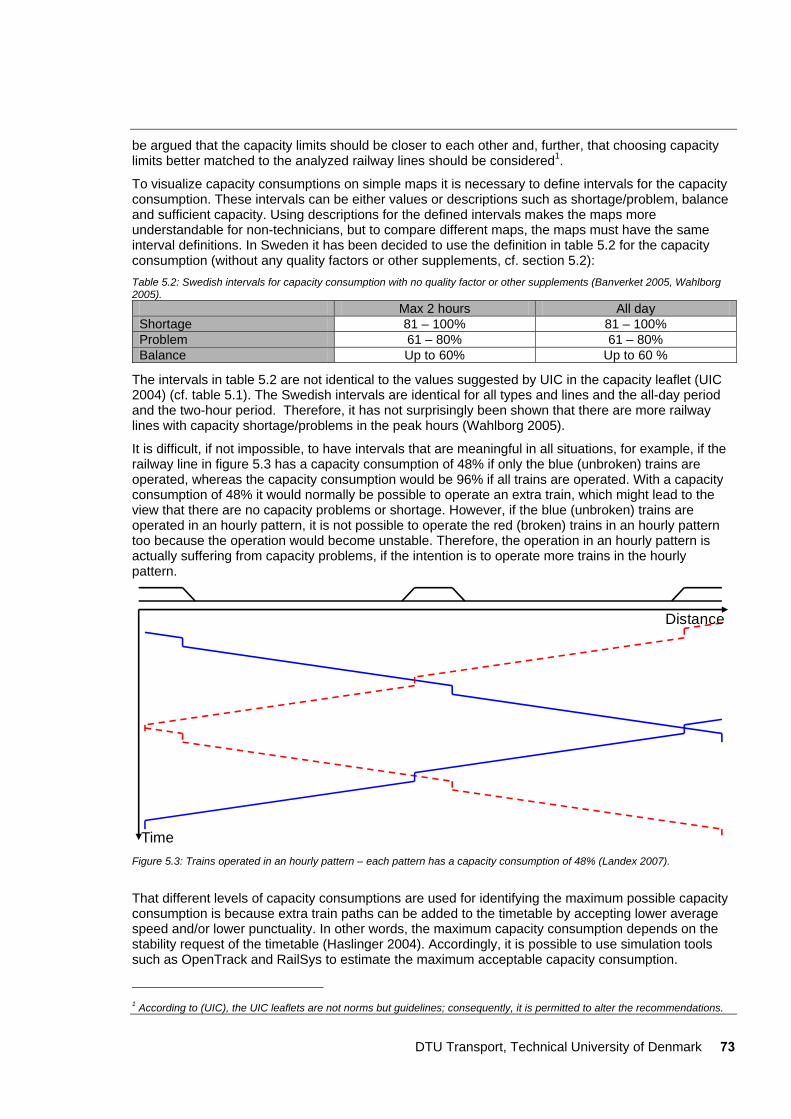
DTU Transport, Technical University of Denmark 73
be argued that the capacity limits should be closer to each other and, further, that choosing capacity limits better matched to the analyzed railway lines should be considered1.
To visualize capacity consumptions on simple maps it is necessary to define intervals for the capacity consumption. These intervals can be either values or descriptions such as shortage/problem, balance and sufficient capacity. Using descriptions for the defined intervals makes the maps more understandable for non-technicians, but to compare different maps, the maps must have the same interval definitions. In Sweden it has been decided to use the definition in table 5.2 for the capacity consumption (without any quality factors or other supplements, cf. section 5.2): Table 5.2: Swedish intervals for capacity consumption with no quality factor or other supplements (Banverket 2005, Wahlborg 2005).
Max 2 hours All day Shortage 81 – 100% 81 – 100% Problem 61 – 80% 61 – 80% Balance Up to 60% Up to 60 %
The intervals in table 5.2 are not identical to the values suggested by UIC in the capacity leaflet (UIC 2004) (cf. table 5.1). The Swedish intervals are identical for all types and lines and the all-day period and the two-hour period. Therefore, it has not surprisingly been shown that there are more railway lines with capacity shortage/problems in the peak hours (Wahlborg 2005).
It is difficult, if not impossible, to have intervals that are meaningful in all situations, for example, if the railway line in figure 5.3 has a capacity consumption of 48% if only the blue (unbroken) trains are operated, whereas the capacity consumption would be 96% if all trains are operated. With a capacity consumption of 48% it would normally be possible to operate an extra train, which might lead to the view that there are no capacity problems or shortage. However, if the blue (unbroken) trains are operated in an hourly pattern, it is not possible to operate the red (broken) trains in an hourly pattern too because the operation would become unstable. Therefore, the operation in an hourly pattern is actually suffering from capacity problems, if the intention is to operate more trains in the hourly pattern.
Distance
Time Figure 5.3: Trains operated in an hourly pattern – each pattern has a capacity consumption of 48% (Landex 2007).
That different levels of capacity consumptions are used for identifying the maximum possible capacity consumption is because extra train paths can be added to the timetable by accepting lower average speed and/or lower punctuality. In other words, the maximum capacity consumption depends on the stability request of the timetable (Haslinger 2004). Accordingly, it is possible to use simulation tools such as OpenTrack and RailSys to estimate the maximum acceptable capacity consumption.
1 According to (UIC), the UIC leaflets are not norms but guidelines; consequently, it is permitted to alter the recommendations.
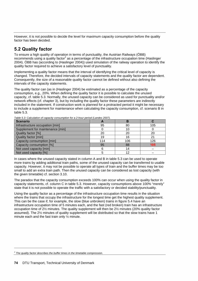
74 DTU Transport, Technical University of Denmark
However, it is not possible to decide the level for maximum capacity consumption before the quality factor has been decided.
5.2 Quality factor To ensure a high quality of operation in terms of punctuality, the Austrian Railways (ÖBB) recommends using a quality factor2 as a percentage of the infrastructure occupation time (Haslinger 2004). ÖBB has (according to (Haslinger 2004)) used simulation of the railway operation to identify the quality factor required to achieve a satisfactory level of punctuality.
Implementing a quality factor means that the interval of identifying the critical level of capacity is changed. Therefore, the decided intervals of capacity statements and the quality factor are dependent. Consequently, the size of a reasonable quality factor cannot be defined without also defining the intervals of the capacity statements.
The quality factor can (as in (Haslinger 2004) be estimated as a percentage of the capacity consumption, e.g., 20%. When defining the quality factor it is possible to calculate the unused capacity, cf. table 5.3. Normally, the unused capacity can be considered as used for punctuality and/or network effects (cf. chapter 3), but by including the quality factor these parameters are indirectly included in the statement. If construction work is planned for a protracted period it might be necessary to include a supplement for maintenance when calculating the capacity consumption, cf. scenario B in table 5.3. Table 5.3: Calculation of capacity consumption for a 2-hour period (Landex 2007).
Scenario A B C Infrastructure occupation [min] 95 80 105 Supplement for maintenance [min] 0 10 0 Quality factor [%] 20 20 20 Quality factor [min] 19 16 21 Capacity consumption [min] 114 106 126 Capacity consumption [%] 95 88 105 Not used capacity [min] 6 14 – Not used capacity [%] 5 12 –
In cases where the unused capacity stated in column A and B in table 5.3 can be used to operate more trains by adding additional train paths, some of the unused capacity can be transferred to usable capacity. However, it may not be possible to operate all types of train and the buffer times may be too small to add an extra train path. Then the unused capacity can be considered as lost capacity (with the given timetable) cf. section 3.10.
The paradox that the capacity consumption exceeds 100% can occur when using the quality factor in capacity statements, cf. column C in table 5.3. However, capacity consumptions above 100% “merely” state that it is not possible to operate the traffic with a satisfactory or decided stability/punctuality.
Using the quality factor as a percentage of the infrastructure occupation time results in the situation where the trains that occupy the infrastructure for the longest time get the highest quality supplement. This can be the case if, for example, the slow (blue unbroken) trains in figure 5.4 have an infrastructure occupation time of 5 minutes each, and the fast (red broken) train has an infrastructure occupation time of 2½ minutes. The quality supplement will then be 2½ minutes (20% quality factor assumed). The 2½ minutes of quality supplement will be distributed so that the slow trains have 1 minute each and the fast train only ½ minute.
2 The quality factor describes the buffer times in the timetable compression.
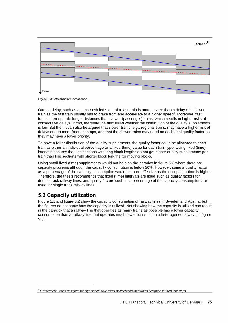
DTU Transport, Technical University of Denmark 75
Distance
Time
Figure 5.4: Infrastructure occupation.
Often a delay, such as an unscheduled stop, of a fast train is more severe than a delay of a slower train as the fast train usually has to brake from and accelerate to a higher speed3. Moreover, fast trains often operate longer distances than slower (passenger) trains, which results in higher risks of consecutive delays. It can, therefore, be discussed whether the distribution of the quality supplements is fair. But then it can also be argued that slower trains, e.g., regional trains, may have a higher risk of delays due to more frequent stops, and that the slower trains may need an additional quality factor as they may have a lower priority.
To have a fairer distribution of the quality supplements, the quality factor could be allocated to each train as either an individual percentage or a fixed (time) value for each train type. Using fixed (time) intervals ensures that line sections with long block lengths do not get higher quality supplements per train than line sections with shorter block lengths (or moving block).
Using small fixed (time) supplements would not help on the paradox in figure 5.3 where there are capacity problems although the capacity consumption is below 50%. However, using a quality factor as a percentage of the capacity consumption would be more effective as the occupation time is higher. Therefore, the thesis recommends that fixed (time) intervals are used such as quality factors for double track railway lines, and quality factors such as a percentage of the capacity consumption are used for single track railway lines.
5.3 Capacity utilization Figure 5.1 and figure 5.2 show the capacity consumption of railway lines in Sweden and Austria, but the figures do not show how the capacity is utilized. Not showing how the capacity is utilized can result in the paradox that a railway line that operates as many trains as possible has a lower capacity consumption than a railway line that operates much fewer trains but in a heterogeneous way, cf. figure 5.5.
3 Furthermore, trains designed for high speed have lower acceleration than trains designed for frequent stops.
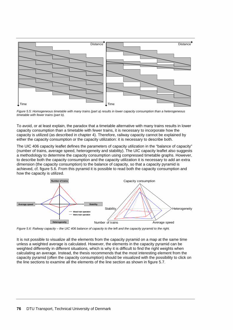
76 DTU Transport, Technical University of Denmark
Distance
Time
Distance
Time Figure 5.5: Homogeneous timetable with many trains (part a) results in lower capacity consumption than a heterogeneous timetable with fewer trains (part b).
To avoid, or at least explain, the paradox that a timetable alternative with many trains results in lower capacity consumption than a timetable with fewer trains, it is necessary to incorporate how the capacity is utilized (as described in chapter 4). Therefore, railway capacity cannot be explained by either the capacity consumption or the capacity utilization: it is necessary to describe both.
The UIC 406 capacity leaflet defines the parameters of capacity utilization in the “balance of capacity” (number of trains, average speed, heterogeneity and stability). The UIC capacity leaflet also suggests a methodology to determine the capacity consumption using compressed timetable graphs. However, to describe both the capacity consumption and the capacity utilization it is necessary to add an extra dimension (the capacity consumption) to the balance of capacity, so that a capacity pyramid is achieved, cf. figure 5.6. From this pyramid it is possible to read both the capacity consumption and how the capacity is utilized.
Average speed StabilityAverage speed Stability
Heterogeneity
Number of trains
Heterogeneity
Number of trains
Mixed train operationMixed train operationMetro train operationMetro train operation
Number of trains
Stability Heterogeneity
Average speed
Capacity consumption
Figure 5.6: Railway capacity – the UIC 406 balance of capacity to the left and the capacity pyramid to the right.
It is not possible to visualize all the elements from the capacity pyramid on a map at the same time unless a weighted average is calculated. However, the elements in the capacity pyramid can be weighted differently in different situations, which is why it is difficult to find the right weights when calculating an average. Instead, the thesis recommends that the most interesting element from the capacity pyramid (often the capacity consumption) should be visualized with the possibility to click on the line sections to examine all the elements of the line section as shown in figure 5.7.
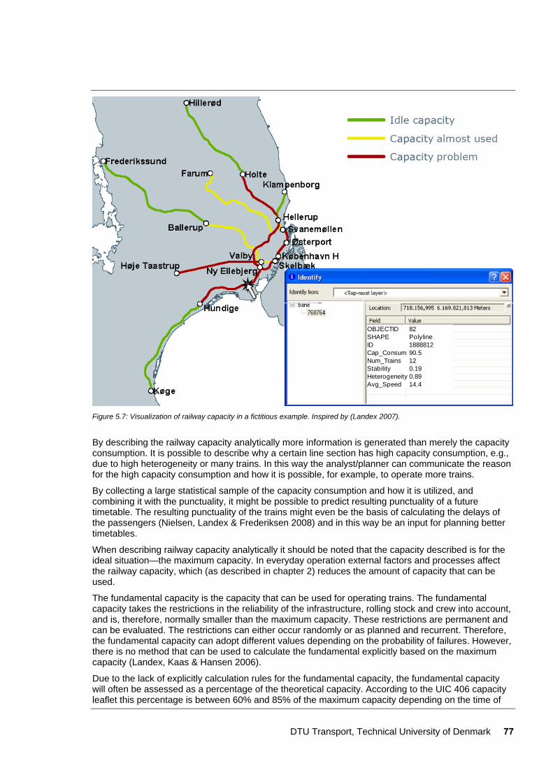
DTU Transport, Technical University of Denmark 77
82Polyline188881290.5120.190.8914.4
OBJECTIDSHAPEIDCap_ConsumNum_TrainsStabilityHeterogeneityAvg_Speed
Figure 5.7: Visualization of railway capacity in a fictitious example. Inspired by (Landex 2007).
By describing the railway capacity analytically more information is generated than merely the capacity consumption. It is possible to describe why a certain line section has high capacity consumption, e.g., due to high heterogeneity or many trains. In this way the analyst/planner can communicate the reason for the high capacity consumption and how it is possible, for example, to operate more trains.
By collecting a large statistical sample of the capacity consumption and how it is utilized, and combining it with the punctuality, it might be possible to predict resulting punctuality of a future timetable. The resulting punctuality of the trains might even be the basis of calculating the delays of the passengers (Nielsen, Landex & Frederiksen 2008) and in this way be an input for planning better timetables.
When describing railway capacity analytically it should be noted that the capacity described is for the ideal situation—the maximum capacity. In everyday operation external factors and processes affect the railway capacity, which (as described in chapter 2) reduces the amount of capacity that can be used.
The fundamental capacity is the capacity that can be used for operating trains. The fundamental capacity takes the restrictions in the reliability of the infrastructure, rolling stock and crew into account, and is, therefore, normally smaller than the maximum capacity. These restrictions are permanent and can be evaluated. The restrictions can either occur randomly or as planned and recurrent. Therefore, the fundamental capacity can adopt different values depending on the probability of failures. However, there is no method that can be used to calculate the fundamental explicitly based on the maximum capacity (Landex, Kaas & Hansen 2006).
Due to the lack of explicitly calculation rules for the fundamental capacity, the fundamental capacity will often be assessed as a percentage of the theoretical capacity. According to the UIC 406 capacity leaflet this percentage is between 60% and 85% of the maximum capacity depending on the time of
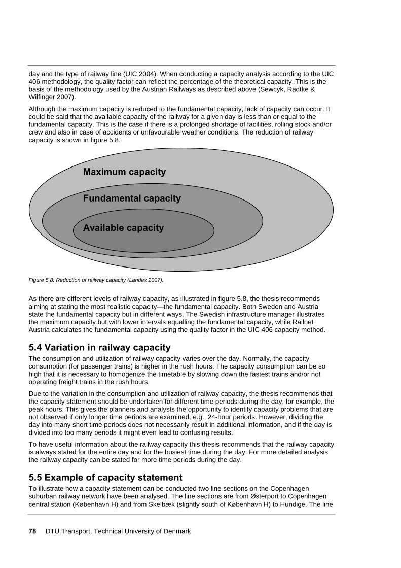
78 DTU Transport, Technical University of Denmark
day and the type of railway line (UIC 2004). When conducting a capacity analysis according to the UIC 406 methodology, the quality factor can reflect the percentage of the theoretical capacity. This is the basis of the methodology used by the Austrian Railways as described above (Sewcyk, Radtke & Wilfinger 2007).
Although the maximum capacity is reduced to the fundamental capacity, lack of capacity can occur. It could be said that the available capacity of the railway for a given day is less than or equal to the fundamental capacity. This is the case if there is a prolonged shortage of facilities, rolling stock and/or crew and also in case of accidents or unfavourable weather conditions. The reduction of railway capacity is shown in figure 5.8.
Available capacity
Fundamental capacity
Maximum capacity
Figure 5.8: Reduction of railway capacity (Landex 2007).
As there are different levels of railway capacity, as illustrated in figure 5.8, the thesis recommends aiming at stating the most realistic capacity—the fundamental capacity. Both Sweden and Austria state the fundamental capacity but in different ways. The Swedish infrastructure manager illustrates the maximum capacity but with lower intervals equalling the fundamental capacity, while Railnet Austria calculates the fundamental capacity using the quality factor in the UIC 406 capacity method.
5.4 Variation in railway capacity The consumption and utilization of railway capacity varies over the day. Normally, the capacity consumption (for passenger trains) is higher in the rush hours. The capacity consumption can be so high that it is necessary to homogenize the timetable by slowing down the fastest trains and/or not operating freight trains in the rush hours.
Due to the variation in the consumption and utilization of railway capacity, the thesis recommends that the capacity statement should be undertaken for different time periods during the day, for example, the peak hours. This gives the planners and analysts the opportunity to identify capacity problems that are not observed if only longer time periods are examined, e.g., 24-hour periods. However, dividing the day into many short time periods does not necessarily result in additional information, and if the day is divided into too many periods it might even lead to confusing results.
To have useful information about the railway capacity this thesis recommends that the railway capacity is always stated for the entire day and for the busiest time during the day. For more detailed analysis the railway capacity can be stated for more time periods during the day.
5.5 Example of capacity statement To illustrate how a capacity statement can be conducted two line sections on the Copenhagen suburban railway network have been analysed. The line sections are from Østerport to Copenhagen central station (København H) and from Skelbæk (slightly south of København H) to Hundige. The line

DTU Transport, Technical University of Denmark 79
section from Østerport to Copenhagen is operated with many trains and has a homogeneous timetable (cf. table 5.4), while the line section from Skelbæk to Hundige is operated with fewer trains but has a heterogeneous timetable (cf. table 5.5). Table 5.4: Timetable for the line section from Østerport to København H (ultimo 2007). The timetable is repeated in 20-minute cycles (DSB S-tog 2007)4.
Train service C+ B E+ A Bx C B+ E A+ H C+ … Østerport 01½ 03½ 05½ 07½ 09½ 11½ 13½ 15½ 17½ 19 21½ … Nørreport 03 05 07 09 11 13 15 17 19 21 23 … Vesterport 05 07 09 11 13 15 17 19 21 23 25 … København H 08 10 12 14 16 18 20 22 24 26 28 …
As seen from the timetable in table 5.4, the line section is operated by 30 trains an hour. However, train service Bx is operated in the peak hours only. All train services except H, which turns around at a separate platform at Østerport, come from the northern suburbs of Copenhagen and continue to the southern part of the suburban railway system5. Table 5.5: Timetable for the line section from Skelbæk to Hundige (ultimo 2007) (DSB S-tog 2007)6.
Train service E A+ E+ A E A+ E+ A E A+ E+ A Skelbæk (05) (07) (15) (17) (25) (27) (35) (37) (45) (47) (55) (57) Sydhavn 07 09 17 19 27 29 37 39 47 49 57 59 Sjælør 08½ 10½ 18½ 20½ 28½ 30½ 38½ 40½ 48½ 50½ 58½ 00½ Ny Ellebjerg 10 12 20 22 30 32 40 42 50 52 00 02 Åmarken | 14½ | 24½ | 34½ | 44½ | 54½ | 04½ Friheden | 16½ | 26½ | 36½ | 46½ | 56½ | 06½ Avedøre | 18½ | 28½ | 38½ | 48½ | 58½ | 08½ Brøndby Strand | 21 | 31 | 41 | 51 | 01 | 11 Vallensbæk | 23 | 33 | 43 | 53 | 03 | 13 Ishøj 18½ 25½ 28½ 35½ 38½ 45½ 48½ 55½ 58½ 05½ 08½ 15½ Hundige 21 29 31 39 41 49 51 59 01 09 11 19
Train services E and E+ (cf. table 5.5) continue from Hundige to Køge, while train lines A and A+ turn around at Hundige station.
The capacity analysis of the 2 railway lines is summarized in table 5.6. The capacity measures are calculated using the methods described in chapter D (the capacity consumption) and chapter E. Table 5.6: Results from capacity analysis of a peak hour7.
Østerport (Kk) → København H (Kh) Skelbæk (Slb) → Hundige (Und)Number of trains 30 trains per hour 12 trains per hour Capacity consumption (K) 92.8% 90.5% Heterogeneity 0.0 0.89 Difference from optimal speed 10 km/h 14.4 km/h Complexity (ϕn) ϕn,Kk = 0.71
ϕn,Kh = 0.50ϕn,Und = 0.75 ϕn,Slb = 0.38
Complexity (ϕp) ϕp,Kk = 0.50 ϕp,Kh = 0.50
ϕp,Und = 0.63 ϕp,Slb = 0.38
Complexity (W) WKk = 0.81 WKh = 0.95
WUnd = 0.44 WSlb = 0.66
Stability (ϕn) 0.15 0.16 Stability (ϕp) 0.25 0.23 Stability (W) 0.01 0.19
4 Train service H has its line end station at Østerport station at a separate platform, which is why it takes longer to drive to Nørreport. 5 Train services C, C+ and H continue to Ballerup and Frederikssund, north of Copenhagen, but this is regarded as the southern part of the suburban railway system as they are driving in a southern direction in Copenhagen. 6 Skelbæk is a technical station without exchange of passengers. 7 The complexity is calculated for trains in both directions. The calculations are done based on the infrastructure from the summer 2007 and an equivalent for the Danish HKT system.
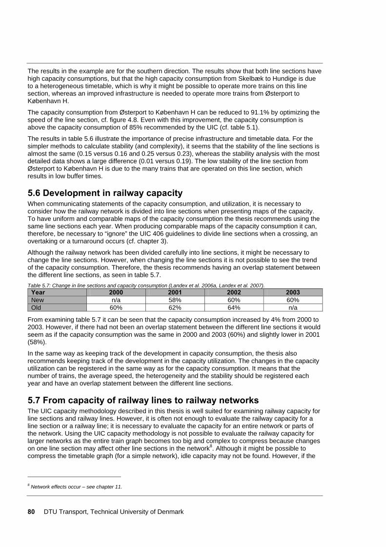
80 DTU Transport, Technical University of Denmark
The results in the example are for the southern direction. The results show that both line sections have high capacity consumptions, but that the high capacity consumption from Skelbæk to Hundige is due to a heterogeneous timetable, which is why it might be possible to operate more trains on this line section, whereas an improved infrastructure is needed to operate more trains from Østerport to København H.
The capacity consumption from Østerport to København H can be reduced to 91.1% by optimizing the speed of the line section, cf. figure 4.8. Even with this improvement, the capacity consumption is above the capacity consumption of 85% recommended by the UIC (cf. table 5.1).
The results in table 5.6 illustrate the importance of precise infrastructure and timetable data. For the simpler methods to calculate stability (and complexity), it seems that the stability of the line sections is almost the same (0.15 versus 0.16 and 0.25 versus 0.23), whereas the stability analysis with the most detailed data shows a large difference (0.01 versus 0.19). The low stability of the line section from Østerport to København H is due to the many trains that are operated on this line section, which results in low buffer times.
5.6 Development in railway capacity When communicating statements of the capacity consumption, and utilization, it is necessary to consider how the railway network is divided into line sections when presenting maps of the capacity. To have uniform and comparable maps of the capacity consumption the thesis recommends using the same line sections each year. When producing comparable maps of the capacity consumption it can, therefore, be necessary to “ignore” the UIC 406 guidelines to divide line sections when a crossing, an overtaking or a turnaround occurs (cf. chapter 3).
Although the railway network has been divided carefully into line sections, it might be necessary to change the line sections. However, when changing the line sections it is not possible to see the trend of the capacity consumption. Therefore, the thesis recommends having an overlap statement between the different line sections, as seen in table 5.7. Table 5.7: Change in line sections and capacity consumption (Landex et al. 2006a, Landex et al. 2007).
Year 2000 2001 2002 2003 New n/a 58% 60% 60% Old 60% 62% 64% n/a
From examining table 5.7 it can be seen that the capacity consumption increased by 4% from 2000 to 2003. However, if there had not been an overlap statement between the different line sections it would seem as if the capacity consumption was the same in 2000 and 2003 (60%) and slightly lower in 2001 (58%).
In the same way as keeping track of the development in capacity consumption, the thesis also recommends keeping track of the development in the capacity utilization. The changes in the capacity utilization can be registered in the same way as for the capacity consumption. It means that the number of trains, the average speed, the heterogeneity and the stability should be registered each year and have an overlap statement between the different line sections.
5.7 From capacity of railway lines to railway networks The UIC capacity methodology described in this thesis is well suited for examining railway capacity for line sections and railway lines. However, it is often not enough to evaluate the railway capacity for a line section or a railway line; it is necessary to evaluate the capacity for an entire network or parts of the network. Using the UIC capacity methodology is not possible to evaluate the railway capacity for larger networks as the entire train graph becomes too big and complex to compress because changes on one line section may affect other line sections in the network8. Although it might be possible to compress the timetable graph (for a simple network), idle capacity may not be found. However, if the
8 Network effects occur – see chapter 11.
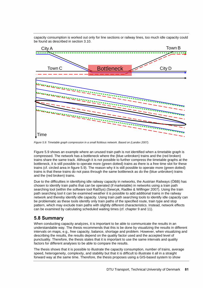
DTU Transport, Technical University of Denmark 81
capacity consumption is worked out only for line sections or railway lines, too much idle capacity could be found as described in section 3.10.
Bottleneck
City A Town B
Town C City D
Time
Figure 5.9: Timetable graph compression in a small fictitious network. Based on (Landex 2007).
Figure 5.9 shows an example where an unused train path is not identified when a timetable graph is compressed. The network has a bottleneck where the (blue unbroken) trains and the (red broken) trains share the same track. Although it is not possible to further compress the timetable graphs at the bottleneck, it is still possible to operate more (green dotted) trains as there is a free time slot for these trains (cf. circled area in figure 5.9). The reason why it is still possible to operate more (green dotted) trains is that these trains do not pass through the same bottleneck as do the (blue unbroken) trains and the (red broken) trains.
Due to the difficulties in identifying idle railway capacity in networks, the Austrian Railways (ÖBB) has chosen to identify train paths that can be operated (if marketable) in networks using a train path searching tool (within the software tool RailSys) (Sewcyk, Radtke & Wilfinger 2007). Using the train path searching tool it can be examined weather it is possible to add additional trains in the railway network and thereby identify idle capacity. Using train path searching tools to identify idle capacity can be problematic as these tools identify only train paths of the specified route, train type and stop pattern, which may exclude train paths with slightly different characteristics. Instead, network effects can be examined by calculating scheduled waiting times (cf. chapter 9 and 11).
5.8 Summary When conducting capacity analyzes, it is important to be able to communicate the results in an understandable way. The thesis recommends that this is be done by visualizing the results in different intervals on maps, e.g., free capacity, balance, shortage and problem. However, when visualizing and describing the results, the results depend on the quality factor used and the accepted level of punctuality. Therefore, the thesis states that it is important to use the same intervals and quality factors for different analyses to be able to compare the results.
The thesis shows that it is possible to illustrate the capacity consumption, number of trains, average speed, heterogeneity, complexity, and stability but that it is difficult to illustrate it all in a straight forward way at the same time. Therefore, the thesis proposes using a GIS-based system to show

82 DTU Transport, Technical University of Denmark
maps of the capacity with the possibility to click on a line section to obtain details of the analytic measurements recommended in chapter 4 (number of trains, average speed, heterogeneity, and stability) of how the capacity is utilized.
If changes are made in the way of stating railway capacity, the line sections or the methodology behind the calculations, the thesis recommends documenting the changes and making overlapping statements in order to be able to compare the results over time.
DTU Transport, Technical University of Denmark 83
Chapter 6
6 Capacity in the case of contingency operation The previous chapters presented how the UIC 406 capacity method can be used for capacity analysis. This chapter shows examples of how the UIC 406 capacity method can be used to examine the effects on the railway capacity in the case of contingency operation. The capacity analysis can be done by all timetabling systems that have conflict detection, such as RailSys (Siefer, Radtke 2005), OpenTrack (Nash, Huerlimann 2004), and STRAX/TPS, which is used by the Danish railway agencies (Kaas, Goossmann 2004), or SIMU, which is used by the Austrian railways (ÖBB) (Höllmüller, Klahn 2005).
Examining capacity in the case of contingency operation is similar to traditional capacity analysis. From a metrological viewpoint, the only differences are the layout of the infrastructure (number of tracks, speed limits, etc.) and the timetables (running times, track usage, number of trains, etc.) examined.
Section 6.1 describes the situation when it is necessary to go from double track operation to single track operation in cases of possessions, e.g., due to maintenance/construction work, accidents or breakdowns. Section 6.1.1 describes how to plan the location of crossovers for fixed interval timetables according to the UIC 406 capacity method, while section 6.1.2 describes how bundled operation can improve the capacity of the railway line in case of a reduced number of tracks. Section 6.1.3 describes the need to change the timetables for contingency operation. Section 6.2 describes the effects on the capacity of railway lines in case of reduced speed, and section 6.3 summarizes the chapter.
6.1 Unscheduled single track operation Not all single track operation is planned. In the case of construction works, a breakdown of a train, or a failure of the signalling or power supply system on a double track line, it may be necessary to close one track and operate the other track in both directions instead. Suitably located crossovers (at stations) on the double track line enable a fast switch from single to bidirectional traffic.
Double track railway lines generally operate more trains than do single track lines. In cases of single track operation on a double track line, it may, therefore, be beneficial to bundle the trains running in one direction before the trains in the other direction follow. Additionally, it may be necessary to change the timetables and/or cancel some of the scheduled trains.
Single-track operation is more complicated than double-track operation. This complexity of single-track operation has been a source of inspiration for many timetable models (Ghoseiri, Szidarovszky & Asgharpour 2004, Zhou, Zhong 2007) and optimisation models (Dorfman, Medanic 2004). These timetable and optimisation models attempt to maximise the number of trains. However, the models insufficiently consider the impacts of the constraints on the capacity consumption due to the track layout and signalling system of the railway lines. This may lead to underestimation of consecutive delays (Landex 2009).
Different approaches can be adopted to reschedule the traffic during disturbances. Optimization approaches to rescheduling during disturbances are described in (D'Ariano 2008, Dorfman, Medanic 2004, Törnquist, Persson 2007). To date, they do not take the additional capacity consumption, and thus risk of consecutive delays, during contingency operations into account.
Furthermore, decision support tools based on optimization approaches remain rarely available in existing traffic control centres, where dispatching is done manually.
6.1.1 Need for crossovers Where to place the crossovers depends on whether the trains are scheduled at fixed intervals that do not change often or whether the trains operate at very different headways.
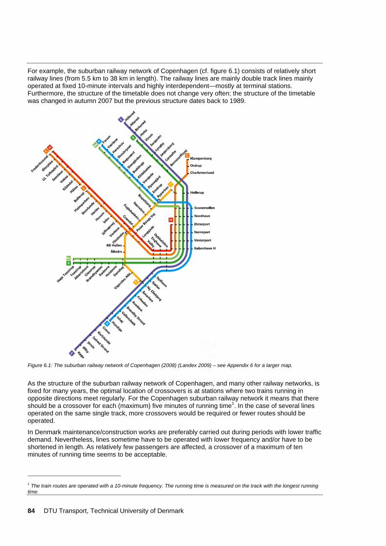
84 DTU Transport, Technical University of Denmark
For example, the suburban railway network of Copenhagen (cf. figure 6.1) consists of relatively short railway lines (from 5.5 km to 38 km in length). The railway lines are mainly double track lines mainly operated at fixed 10-minute intervals and highly interdependent—mostly at terminal stations. Furthermore, the structure of the timetable does not change very often; the structure of the timetable was changed in autumn 2007 but the previous structure dates back to 1989.
Figure 6.1: The suburban railway network of Copenhagen (2008) (Landex 2009) – see Appendix 6 for a larger map.
As the structure of the suburban railway network of Copenhagen, and many other railway networks, is fixed for many years, the optimal location of crossovers is at stations where two trains running in opposite directions meet regularly. For the Copenhagen suburban railway network it means that there should be a crossover for each (maximum) five minutes of running time1. In the case of several lines operated on the same single track, more crossovers would be required or fewer routes should be operated.
In Denmark maintenance/construction works are preferably carried out during periods with lower traffic demand. Nevertheless, lines sometime have to be operated with lower frequency and/or have to be shortened in length. As relatively few passengers are affected, a crossover of a maximum of ten minutes of running time seems to be acceptable.
1 The train routes are operated with a 10-minute frequency. The running time is measured on the track with the longest running time.
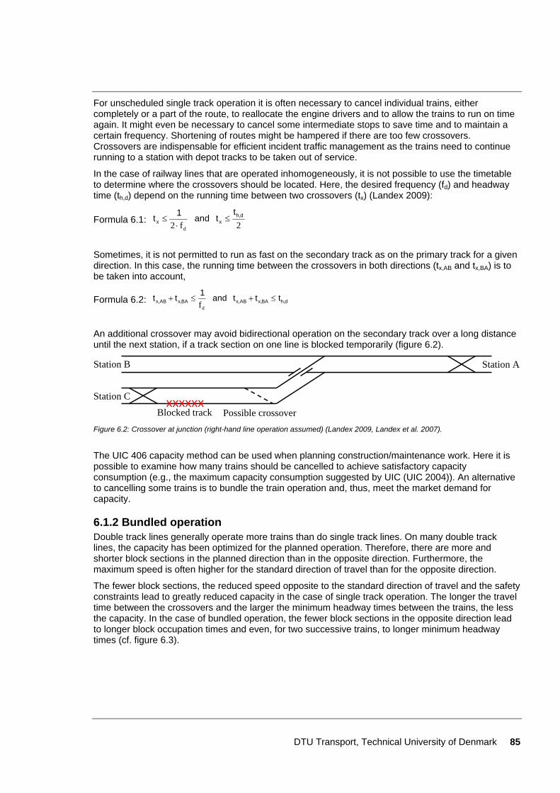
DTU Transport, Technical University of Denmark 85
For unscheduled single track operation it is often necessary to cancel individual trains, either completely or a part of the route, to reallocate the engine drivers and to allow the trains to run on time again. It might even be necessary to cancel some intermediate stops to save time and to maintain a certain frequency. Shortening of routes might be hampered if there are too few crossovers. Crossovers are indispensable for efficient incident traffic management as the trains need to continue running to a station with depot tracks to be taken out of service.
In the case of railway lines that are operated inhomogeneously, it is not possible to use the timetable to determine where the crossovers should be located. Here, the desired frequency (fd) and headway time (th,d) depend on the running time between two crossovers (tx) (Landex 2009):
Formula 6.1: 2f2 d
dh,xx
tt and 1t ≤
⋅≤
Sometimes, it is not permitted to run as fast on the secondary track as on the primary track for a given direction. In this case, the running time between the crossovers in both directions (tx,AB and tx,BA) is to be taken into account,
Formula 6.2: dh,BAx,ABx,BAx,ABx, ttt and 1tt ≤+≤+df
An additional crossover may avoid bidirectional operation on the secondary track over a long distance until the next station, if a track section on one line is blocked temporarily (figure 6.2).
Station AStation B
Station C
Blocked trackxxxxxx
Possible crossover Figure 6.2: Crossover at junction (right-hand line operation assumed) (Landex 2009, Landex et al. 2007).
The UIC 406 capacity method can be used when planning construction/maintenance work. Here it is possible to examine how many trains should be cancelled to achieve satisfactory capacity consumption (e.g., the maximum capacity consumption suggested by UIC (UIC 2004)). An alternative to cancelling some trains is to bundle the train operation and, thus, meet the market demand for capacity.
6.1.2 Bundled operation Double track lines generally operate more trains than do single track lines. On many double track lines, the capacity has been optimized for the planned operation. Therefore, there are more and shorter block sections in the planned direction than in the opposite direction. Furthermore, the maximum speed is often higher for the standard direction of travel than for the opposite direction.
The fewer block sections, the reduced speed opposite to the standard direction of travel and the safety constraints lead to greatly reduced capacity in the case of single track operation. The longer the travel time between the crossovers and the larger the minimum headway times between the trains, the less the capacity. In the case of bundled operation, the fewer block sections in the opposite direction lead to longer block occupation times and even, for two successive trains, to longer minimum headway times (cf. figure 6.3).
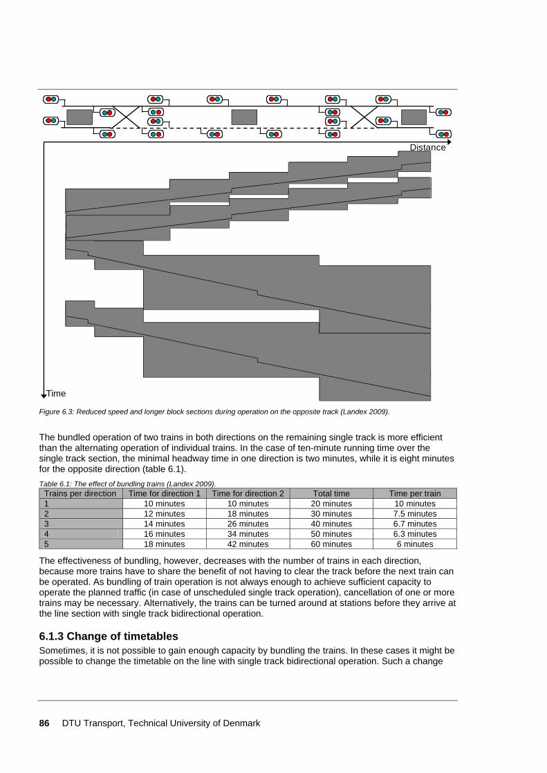
86 DTU Transport, Technical University of Denmark
Distance
Time
Figure 6.3: Reduced speed and longer block sections during operation on the opposite track (Landex 2009).
The bundled operation of two trains in both directions on the remaining single track is more efficient than the alternating operation of individual trains. In the case of ten-minute running time over the single track section, the minimal headway time in one direction is two minutes, while it is eight minutes for the opposite direction (table 6.1). Table 6.1: The effect of bundling trains (Landex 2009).
Trains per direction Time for direction 1 Time for direction 2 Total time Time per train 1 10 minutes 10 minutes 20 minutes 10 minutes 2 12 minutes 18 minutes 30 minutes 7.5 minutes 3 14 minutes 26 minutes 40 minutes 6.7 minutes 4 16 minutes 34 minutes 50 minutes 6.3 minutes 5 18 minutes 42 minutes 60 minutes 6 minutes
The effectiveness of bundling, however, decreases with the number of trains in each direction, because more trains have to share the benefit of not having to clear the track before the next train can be operated. As bundling of train operation is not always enough to achieve sufficient capacity to operate the planned traffic (in case of unscheduled single track operation), cancellation of one or more trains may be necessary. Alternatively, the trains can be turned around at stations before they arrive at the line section with single track bidirectional operation.
6.1.3 Change of timetables Sometimes, it is not possible to gain enough capacity by bundling the trains. In these cases it might be possible to change the timetable on the line with single track bidirectional operation. Such a change
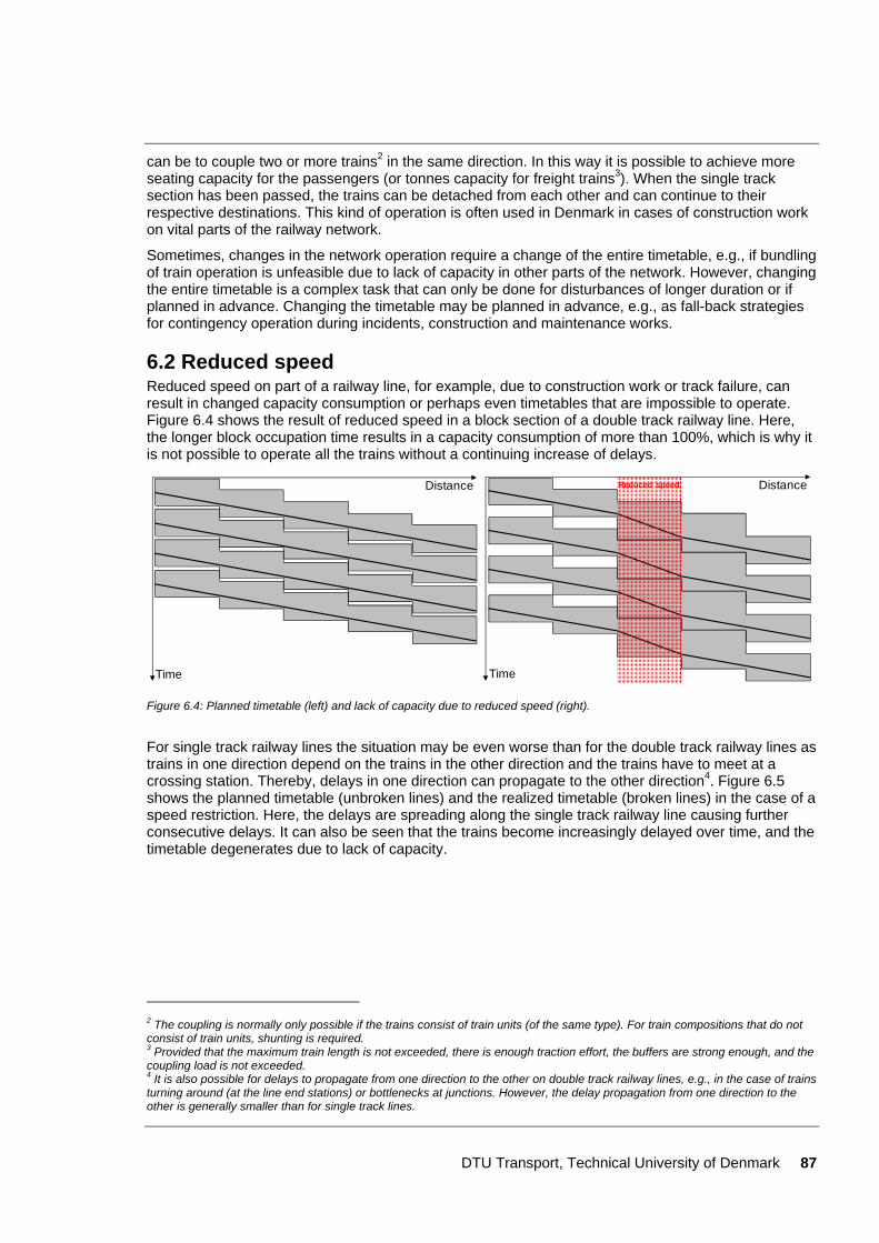
DTU Transport, Technical University of Denmark 87
can be to couple two or more trains2 in the same direction. In this way it is possible to achieve more seating capacity for the passengers (or tonnes capacity for freight trains3). When the single track section has been passed, the trains can be detached from each other and can continue to their respective destinations. This kind of operation is often used in Denmark in cases of construction work on vital parts of the railway network.
Sometimes, changes in the network operation require a change of the entire timetable, e.g., if bundling of train operation is unfeasible due to lack of capacity in other parts of the network. However, changing the entire timetable is a complex task that can only be done for disturbances of longer duration or if planned in advance. Changing the timetable may be planned in advance, e.g., as fall-back strategies for contingency operation during incidents, construction and maintenance works.
6.2 Reduced speed Reduced speed on part of a railway line, for example, due to construction work or track failure, can result in changed capacity consumption or perhaps even timetables that are impossible to operate. Figure 6.4 shows the result of reduced speed in a block section of a double track railway line. Here, the longer block occupation time results in a capacity consumption of more than 100%, which is why it is not possible to operate all the trains without a continuing increase of delays.
Distance
Time
Distance
Time
Reduced speed
Figure 6.4: Planned timetable (left) and lack of capacity due to reduced speed (right).
For single track railway lines the situation may be even worse than for the double track railway lines as trains in one direction depend on the trains in the other direction and the trains have to meet at a crossing station. Thereby, delays in one direction can propagate to the other direction4. Figure 6.5 shows the planned timetable (unbroken lines) and the realized timetable (broken lines) in the case of a speed restriction. Here, the delays are spreading along the single track railway line causing further consecutive delays. It can also be seen that the trains become increasingly delayed over time, and the timetable degenerates due to lack of capacity.
2 The coupling is normally only possible if the trains consist of train units (of the same type). For train compositions that do not consist of train units, shunting is required. 3 Provided that the maximum train length is not exceeded, there is enough traction effort, the buffers are strong enough, and the coupling load is not exceeded. 4 It is also possible for delays to propagate from one direction to the other on double track railway lines, e.g., in the case of trains turning around (at the line end stations) or bottlenecks at junctions. However, the delay propagation from one direction to the other is generally smaller than for single track lines.
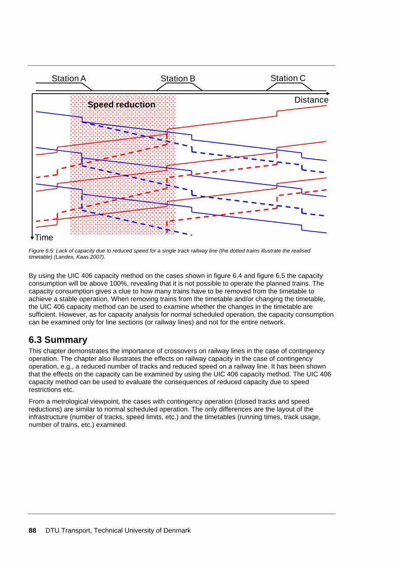
88 DTU Transport, Technical University of Denmark
Distance
Time
Station A Station B Station C
Speed reduction
Figure 6.5: Lack of capacity due to reduced speed for a single track railway line (the dotted trains illustrate the realised timetable) (Landex, Kaas 2007).
By using the UIC 406 capacity method on the cases shown in figure 6.4 and figure 6.5 the capacity consumption will be above 100%, revealing that it is not possible to operate the planned trains. The capacity consumption gives a clue to how many trains have to be removed from the timetable to achieve a stable operation. When removing trains from the timetable and/or changing the timetable, the UIC 406 capacity method can be used to examine whether the changes in the timetable are sufficient. However, as for capacity analysis for normal scheduled operation, the capacity consumption can be examined only for line sections (or railway lines) and not for the entire network.
6.3 Summary This chapter demonstrates the importance of crossovers on railway lines in the case of contingency operation. The chapter also illustrates the effects on railway capacity in the case of contingency operation, e.g., a reduced number of tracks and reduced speed on a railway line. It has been shown that the effects on the capacity can be examined by using the UIC 406 capacity method. The UIC 406 capacity method can be used to evaluate the consequences of reduced capacity due to speed restrictions etc.
From a metrological viewpoint, the cases with contingency operation (closed tracks and speed reductions) are similar to normal scheduled operation. The only differences are the layout of the infrastructure (number of tracks, speed limits, etc.) and the timetables (running times, track usage, number of trains, etc.) examined.
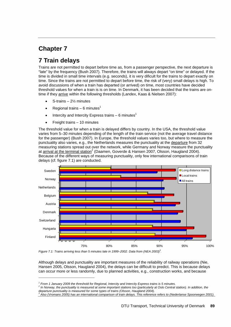
DTU Transport, Technical University of Denmark 89
Chapter 7
7 Train delays Trains are not permitted to depart before time as, from a passenger perspective, the next departure is “late” by the frequency (Bush 2007). Therefore, the trains will always depart “on time” or delayed. If the time is divided in small time intervals (e.g. seconds), it is very dificult for the trains to depart exactly on time. Since the trains are not permitted to depart before time, the risk of (very) small delays is high. To avoid discussions of when a train has departed (or arrived) on time, most countries have decided threshold values for when a train is is on time. In Denmark, it has been decided that the trains are on-time if they arrive within the following thresholds (Landex, Kaas & Nielsen 2007):
• S-trains – 2½ minutes
• Regional trains – 6 minutes1
• Intercity and Intercity Express trains – 6 minutes1
• Freight trains – 10 minutes
The threshold value for when a train is delayed differs by country. In the USA, the threshold value varies from 5–30 minutes depending of the length of the train service (not the average travel distance for the passenger) (Bush 2007). In Europe, the threshold values varies too, but where to measure the punctuality also varies, e.g., the Netherlands measures the punctuality at the departure from 32 measuring stations spread out over the network, while Germany and Norway measure the punctuality at arrival at the terminal station2 (Daamen, Goverde & Hansen 2007, Olsson, Haugland 2004). Because of the different ways of measuring punctuality, only few international comparisons of train delays (cf. figure 7.1) are conducted.
70% 75% 80% 85% 90% 95% 100%
Finland
Hungaria
Switzerland
Denmark
Austria
Belgium
Netherlands
Norway
Sweden Long distance trains
Local trains
All trains
Figure 7.1: Trains arriving less than 5 minutes late in 1999–2002. Data from (NEA 2003)3.
Although delays and punctuality are important measures of the reliability of railway operations (Nie, Hansen 2005, Olsson, Haugland 2004), the delays can be difficult to predict. This is because delays can occur more or less randomly, due to planned activities, e.g., construction works, and because 1 From 1 January 2009 the threshold for Regional, Intercity and Intercity Express trains is 5 minutes. 2 In Norway, the punctuality is measured at some important stations too (particularly at Oslo Central station). In addition, the departure punctuality is measured for some types of trains (Olsson, Haugland 2004). 3 Also (Vromans 2005) has an international comparison of train delays. This reference refers to (Nederlanse Spoorwegen 2001).
90 DTU Transport, Technical University of Denmark
delayed trains may delay other trains. Section 7.1 gives a general introduction to the different types of delay. Then section 7.2 describes how the capacity consumption affects the delay propagation.
Section 7.3 describes the delay propagation in detail for the ideal case of hemogeneous operation on a double track line, while section 7.4 describes the cases of heterogeneous double track operation and single track operation. As the complexity of delay calculations increases with the size of the network and the complexity of the operation, section 7.5 describes how delays can be found by simulation. Lastly, section 7.6, summarizes the the chapter.
7.1 Delays Delays in railway operation can be divided into initial and consecutive delays (Carey, Kwiecinski 1994, Hansen 2004a). Initial delays are the original delays caused by a delay for a single train, and the consecutive delays are delays caused by other (delayed) trains. The initial delays normally occur due to longer time for exchange of passengers, e.g., due to many passengers, or to passengers who require extra help to board/alight the train; errors on the infrastructure or the rolling stock; and weather conditions. The total amount of delays in the railway system (Σtd) is equal to the sum of consecutive delays (Σtd,x,c) and the initial delay (td,1,i):
Formula 7.1: ∑=
+=∑X
2xc,x,di,1dd ttt
The reasons for initial delays that can be related to the infrastructure or the rolling stock will generally be regarded as technical errors. The duration of the technical errors plays an important role with respect to the consequences. Regarding the rolling stock, the errors can be divided as shown in table 7.1: Table 7.1: Errors regarding the rolling stock. Based on (Kaas 1998b, Landex, Kaas & Hansen 2006, Skartsæterhagen 1993).
Type of error Description of errorTemporary error The error is corrected immediately, and it is (most often) not
necessary to take operational actions, e.g. that other trains overtake the train with technical problems.
Permenent error, but the train can continue
Typically, it will be necessary to reduce the speed, e.g. because of reduced traction power.
Long-lasting error, where the train cannot continue
Until the train is taken out of the system or the error is corrected, the infrastructure is occupied by the train and cannot be used by other trains. Depending on the free capacity of the line, this line obstruction will cause major or minor troubles in the operation.
Correspondingly, errors in the infrastructure can be grouped as shown in table 7.2: Table 7.2: Errors regarding the infrastructure. Based on (Kaas 1998b, Landex, Kaas & Hansen 2006, Skartsæterhagen 1993).
Type of error Description of error Temporary error The error is corrected immediately. It may e.g. be due to signal
problems, where the driver must call on the radio to find out if the train can continue.
Permenently reduced capacity If the limitations of the infrastructure are prolonged, the traffic must be rerouted. It may be necessary to introduce single track operation on a double track line, if one track is not available.
Total closure of the traffic If all the tracks on the line are blocked, the traffic can only be re-established when the error has been corrected.
All the above types of technical error result in a limitation of the available capacity, as compared with the fundamental capacity that can be obtained under normal conditions (cf. section 5.4). In the case of long-lasting limitations of the infrastructure or the rolling stock properties, these can be included in the system examined, after which it is possible to carry out a capacity analysis based on the new prerequisites. In contrast, temporary technical errors should be examined in the original system, where the delay propagation from one train to a successive train can be followed.
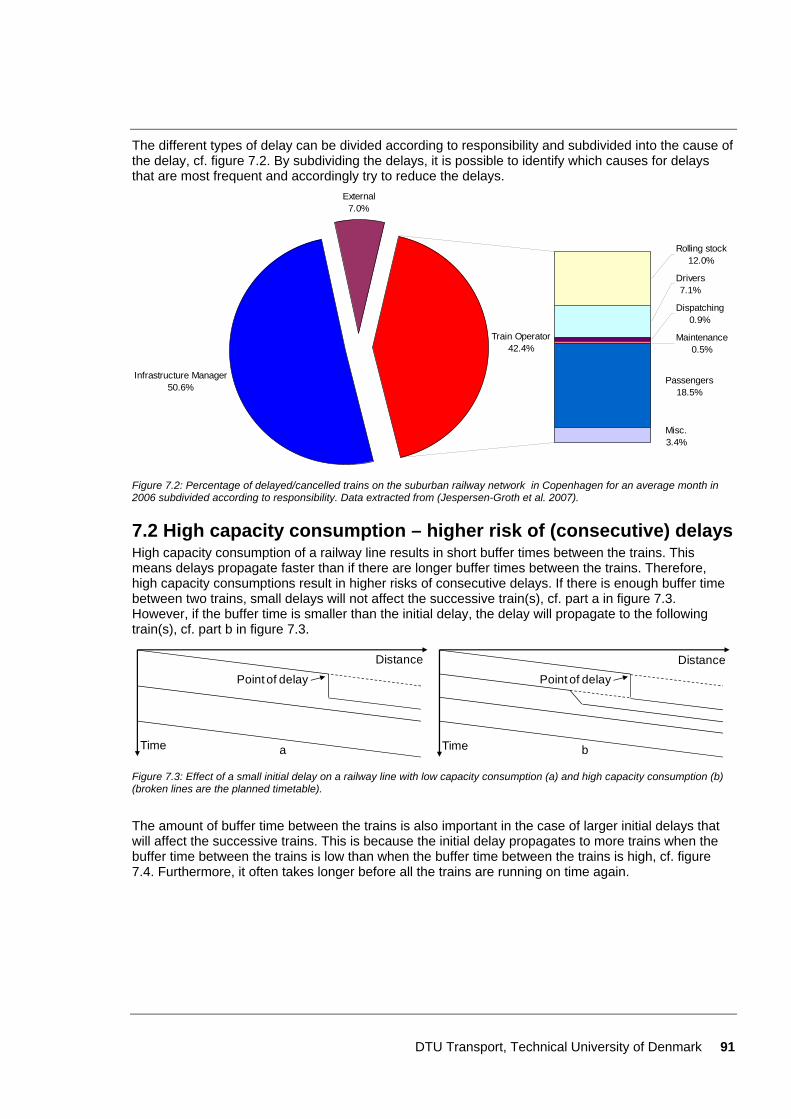
DTU Transport, Technical University of Denmark 91
The different types of delay can be divided according to responsibility and subdivided into the cause of the delay, cf. figure 7.2. By subdividing the delays, it is possible to identify which causes for delays that are most frequent and accordingly try to reduce the delays.
Infrastructure Manager50.6%
Rolling stock12.0%
Drivers7.1%
Dispatching0.9%
Maintenance0.5%
Passengers18.5%
Train Operator42.4%
External7.0%
Misc.3.4%
Figure 7.2: Percentage of delayed/cancelled trains on the suburban railway network in Copenhagen for an average month in 2006 subdivided according to responsibility. Data extracted from (Jespersen-Groth et al. 2007).
7.2 High capacity consumption – higher risk of (consecutive) delays High capacity consumption of a railway line results in short buffer times between the trains. This means delays propagate faster than if there are longer buffer times between the trains. Therefore, high capacity consumptions result in higher risks of consecutive delays. If there is enough buffer time between two trains, small delays will not affect the successive train(s), cf. part a in figure 7.3. However, if the buffer time is smaller than the initial delay, the delay will propagate to the following train(s), cf. part b in figure 7.3.
Time
DistancePoint of delay
Time
Distance
Point of delay
a b Figure 7.3: Effect of a small initial delay on a railway line with low capacity consumption (a) and high capacity consumption (b) (broken lines are the planned timetable).
The amount of buffer time between the trains is also important in the case of larger initial delays that will affect the successive trains. This is because the initial delay propagates to more trains when the buffer time between the trains is low than when the buffer time between the trains is high, cf. figure 7.4. Furthermore, it often takes longer before all the trains are running on time again.
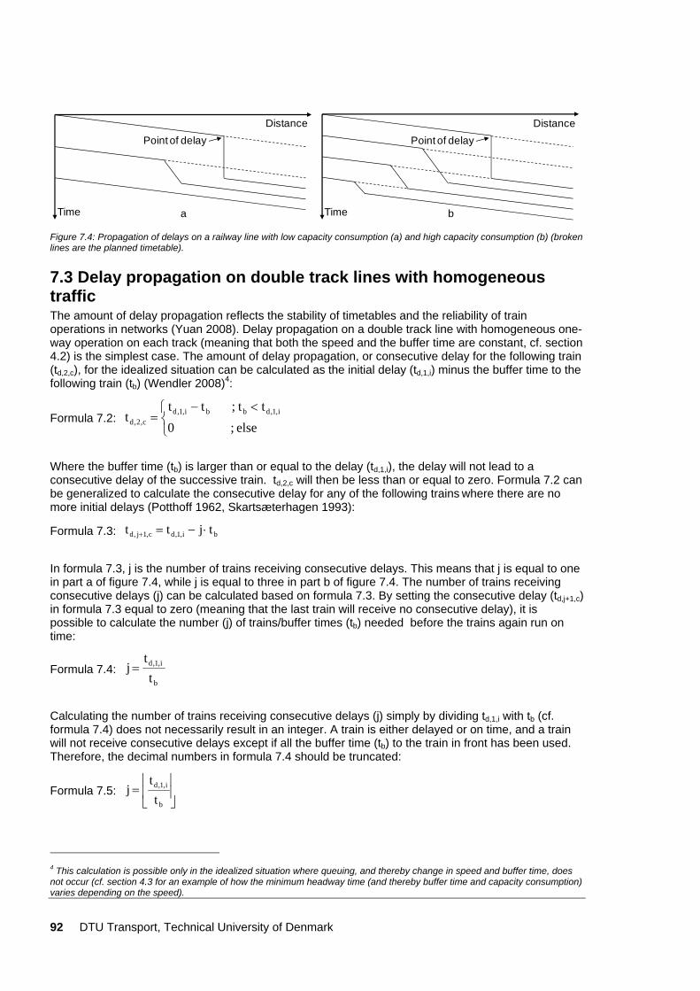
92 DTU Transport, Technical University of Denmark
Time
DistancePoint of delay
Time
DistancePoint of delay
a b Figure 7.4: Propagation of delays on a railway line with low capacity consumption (a) and high capacity consumption (b) (broken lines are the planned timetable).
7.3 Delay propagation on double track lines with homogeneous traffic The amount of delay propagation reflects the stability of timetables and the reliability of train operations in networks (Yuan 2008). Delay propagation on a double track line with homogeneous one-way operation on each track (meaning that both the speed and the buffer time are constant, cf. section 4.2) is the simplest case. The amount of delay propagation, or consecutive delay for the following train (td,2,c), for the idealized situation can be calculated as the initial delay (td,1,i) minus the buffer time to the following train (tb) (Wendler 2008)4:
Formula 7.2: ⎩⎨⎧ <−
=else;0
tt;ttt i,1,dbbi,1,d
c,2,d
Where the buffer time (tb) is larger than or equal to the delay (td,1,i), the delay will not lead to a consecutive delay of the successive train. td,2,c will then be less than or equal to zero. Formula 7.2 can be generalized to calculate the consecutive delay for any of the following trains where there are no more initial delays (Potthoff 1962, Skartsæterhagen 1993):
Formula 7.3: bi,1,dc,1j,d tjtt ⋅−=+
In formula 7.3, j is the number of trains receiving consecutive delays. This means that j is equal to one in part a of figure 7.4, while j is equal to three in part b of figure 7.4. The number of trains receiving consecutive delays (j) can be calculated based on formula 7.3. By setting the consecutive delay (td,j+1,c) in formula 7.3 equal to zero (meaning that the last train will receive no consecutive delay), it is possible to calculate the number (j) of trains/buffer times (tb) needed before the trains again run on time:
Formula 7.4: b
i,1,d
tt
j =
Calculating the number of trains receiving consecutive delays (j) simply by dividing td,1,i with tb (cf. formula 7.4) does not necessarily result in an integer. A train is either delayed or on time, and a train will not receive consecutive delays except if all the buffer time (tb) to the train in front has been used. Therefore, the decimal numbers in formula 7.4 should be truncated:
Formula 7.5: ⎥⎦
⎥⎢⎣
⎢=
b
i,1,d
tt
j
4 This calculation is possible only in the idealized situation where queuing, and thereby change in speed and buffer time, does not occur (cf. section 4.3 for an example of how the minimum headway time (and thereby buffer time and capacity consumption) varies depending on the speed).
DTU Transport, Technical University of Denmark 93
Knowing the number of trains receiving consecutive delays (j), it is possible to calculate the total delay (Σtd) caused by the initial delay (td,1,i) by:
Formula 7.6: ∑+
=+ +=++++=Σ
1j
1xc,x,di,1,dc,1j,dc,2,dc,2,di,1,dd ttt...tttt
Combining formula 7.3 and formula 7.6, the total delay (Σtd) caused by the initial delay (td,1,i) can be calculated as:
Formula 7.7: ( ) ( ) b2j
i,1,dbi,1,dbi,1,dbi,1,di,1,dd t1jt1jtjt...t2ttttt ⋅+⋅−⋅+=⋅−++⋅−+−+=Σ
Combining formula 7.5 and formula 7.7, the total delay (Σtd) can be calculated based on the initial delay (td,1,i) and the buffer time tb:
Formula 7.8: bb
i,1,d
b
i,1,di,1,d
b
i,1,dd t1
tt
tt
21t1
tt
t ⋅⎟⎟⎠
⎞⎜⎜⎝
⎛+⎥
⎦
⎥⎢⎣
⎢⋅⎥⎦
⎥⎢⎣
⎢⋅−⋅⎟⎟
⎠
⎞⎜⎜⎝
⎛+⎥
⎦
⎥⎢⎣
⎢=Σ
For initial delays much larger than the buffer time, formula 7.8 can be simplified to (Potthoff 1962):
Formula 7.9: 2
t1
tt
t i,1,d
b
i,1,dd ⋅⎟⎟
⎠
⎞⎜⎜⎝
⎛+=Σ
The simplification by (Potthoff 1962) in formula 7.9 is not necessarily precise for either small initial delays or large buffer times between the trains. Therefore, the more precise formula 7.8 is used instead.
To examine the influence of high capacity consumption on the delay propagation (and thereby the punctuality) the buffer time5 (tb) can be expressed based on the capacity consumption in per cent (K) and the minimum headway time (th,min) (Landex, Kaas & Hansen 2006, Kaas 1998b, Skartsæterhagen 1993):
Formula 7.10: min,hmin,hmin,h
min,hhb t1K1t
Kt
ttt ⋅⎟⎠⎞
⎜⎝⎛ −=−=−=
The sum of delays (Σtd) can then be expressed as:
Formula 7.11: ( )( )
( ) ( ) ⎟⎟⎠
⎞⎜⎜⎝
⎛+⎥
⎦
⎥⎢⎣
⎢
⋅−⋅⎥⎦
⎥⎢⎣
⎢
⋅−⋅
⋅−−⋅⎟
⎟⎠
⎞⎜⎜⎝
⎛+⎥
⎦
⎥⎢⎣
⎢
⋅−=Σ 1
t1t
t1t
2t1
t1t1
tt
min,hK1
i,1,d
min,hK1
i,1,dmin,hK1
min,hmin,hK
1i,1,d
d
For a railway line with a minimum headway time (th,min) of 3 minutes, the sum of delays (Σtd) can be calculated for various initial delays (td,1,i) and capacity consumptions (K) based on formula 7.11, cf. figure 7.5.
5 The buffer time (tb) can be calculated as the difference between the planned headway time (th) and the minimum headway time (th,min).
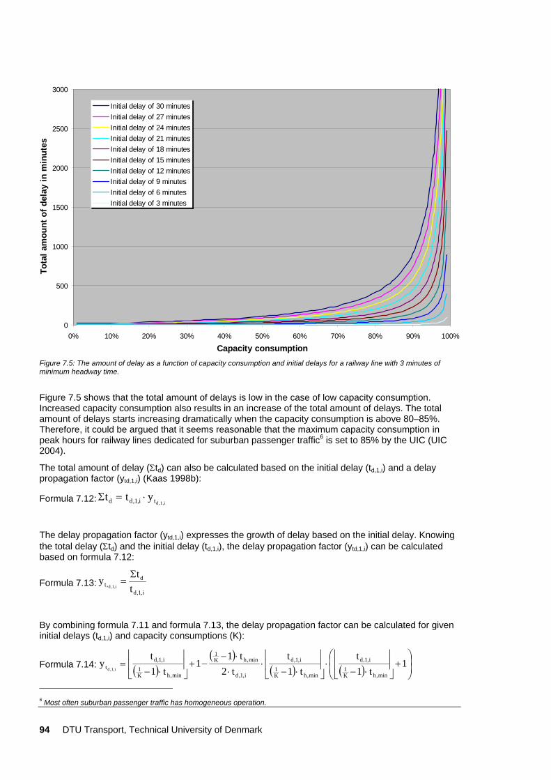
94 DTU Transport, Technical University of Denmark
0
500
1000
1500
2000
2500
3000
0% 10% 20% 30% 40% 50% 60% 70% 80% 90% 100%
Capacity consumption
Tota
l am
ount
of d
elay
in m
inut
es
Initial delay of 30 minutesInitial delay of 27 minutesInitial delay of 24 minutesInitial delay of 21 minutesInitial delay of 18 minutesInitial delay of 15 minutesInitial delay of 12 minutesInitial delay of 9 minutesInitial delay of 6 minutesInitial delay of 3 minutes
Figure 7.5: The amount of delay as a function of capacity consumption and initial delays for a railway line with 3 minutes of minimum headway time.
Figure 7.5 shows that the total amount of delays is low in the case of low capacity consumption. Increased capacity consumption also results in an increase of the total amount of delays. The total amount of delays starts increasing dramatically when the capacity consumption is above 80–85%. Therefore, it could be argued that it seems reasonable that the maximum capacity consumption in peak hours for railway lines dedicated for suburban passenger traffic6 is set to 85% by the UIC (UIC 2004).
The total amount of delay (Σtd) can also be calculated based on the initial delay (td,1,i) and a delay propagation factor (ytd,1,i) (Kaas 1998b):
Formula 7.12: i,1,dti,1,dd ytt ⋅=Σ
The delay propagation factor (ytd,1,i) expresses the growth of delay based on the initial delay. Knowing the total delay (Σtd) and the initial delay (td,1,i), the delay propagation factor (ytd,1,i) can be calculated based on formula 7.12:
Formula 7.13: i,1,d
d,t t
tyi,1,d
Σ=
By combining formula 7.11 and formula 7.13, the delay propagation factor can be calculated for given initial delays (td,1,i) and capacity consumptions (K):
Formula 7.14: ( )( )
( ) ( ) ⎟⎟⎠
⎞⎜⎜⎝
⎛+⎥
⎦
⎥⎢⎣
⎢
⋅−⋅⎥⎦
⎥⎢⎣
⎢
⋅−⋅
⋅⋅−
−+⎥⎦
⎥⎢⎣
⎢
⋅−= 1
t1t
t1t
t2t1
1t1
ty
min,hK1
i,1,d
min,hK1
i,1,d
i,1,d
min,hK1
min,hK1
i,1,dt i,1,d
6 Most often suburban passenger traffic has homogeneous operation.
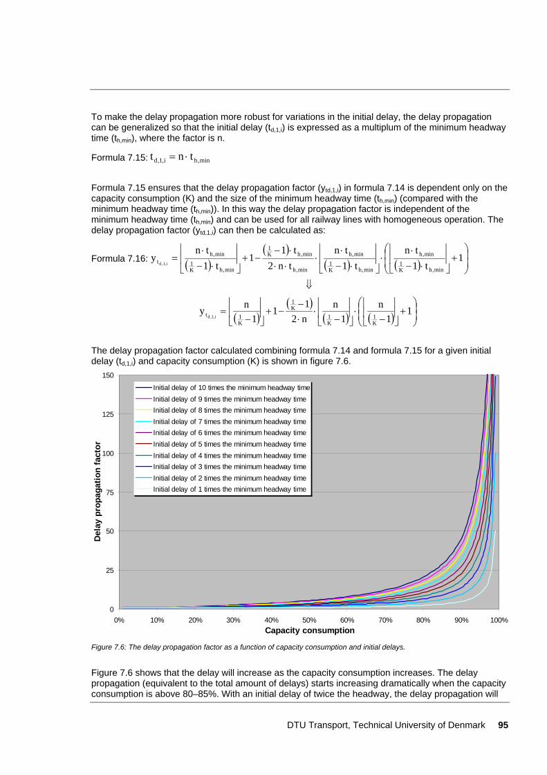
DTU Transport, Technical University of Denmark 95
To make the delay propagation more robust for variations in the initial delay, the delay propagation can be generalized so that the initial delay (td,1,i) is expressed as a multiplum of the minimum headway time (th,min), where the factor is n.
Formula 7.15: min,hi,1,d tnt ⋅=
Formula 7.15 ensures that the delay propagation factor (ytd,1,i) in formula 7.14 is dependent only on the capacity consumption (K) and the size of the minimum headway time (th,min) (compared with the minimum headway time (th,min)). In this way the delay propagation factor is independent of the minimum headway time (th,min) and can be used for all railway lines with homogeneous operation. The delay propagation factor (ytd,1,i) can then be calculated as:
Formula 7.16:
( )( )
( ) ( )
( )( )
( ) ( ) ⎟⎟⎠
⎞⎜⎜⎝
⎛+⎥
⎦
⎥⎢⎣
⎢−
⋅⎥⎦
⎥⎢⎣
⎢−
⋅⋅−
−+⎥⎦
⎥⎢⎣
⎢−
=
⇓
⎟⎟⎠
⎞⎜⎜⎝
⎛+⎥
⎦
⎥⎢⎣
⎢
⋅−⋅
⋅⎥⎦
⎥⎢⎣
⎢
⋅−⋅
⋅⋅⋅⋅−
−+⎥⎦
⎥⎢⎣
⎢
⋅−⋅
=
11
n1
nn21
11
ny
1t1
tnt1
tntn2t1
1t1
tny
K1
K1
K1
K1t
min,hK1
min,h
min,hK1
min,h
min,h
min,hK1
min,hK1
min,ht
i,1,d
i,1,d
The delay propagation factor calculated combining formula 7.14 and formula 7.15 for a given initial delay (td,1,i) and capacity consumption (K) is shown in figure 7.6.
0
25
50
75
100
125
150
0% 10% 20% 30% 40% 50% 60% 70% 80% 90% 100%Capacity consumption
Del
ay p
ropa
gatio
n fa
ctor
Initial delay of 10 times the minimum headway timeInitial delay of 9 times the minimum headway timeInitial delay of 8 times the minimum headway timeInitial delay of 7 times the minimum headway timeInitial delay of 6 times the minimum headway timeInitial delay of 5 times the minimum headway timeInitial delay of 4 times the minimum headway timeInitial delay of 3 times the minimum headway timeInitial delay of 2 times the minimum headway timeInitial delay of 1 times the minimum headway time
Figure 7.6: The delay propagation factor as a function of capacity consumption and initial delays.
Figure 7.6 shows that the delay will increase as the capacity consumption increases. The delay propagation (equivalent to the total amount of delays) starts increasing dramatically when the capacity consumption is above 80–85%. With an initial delay of twice the headway, the delay propagation will
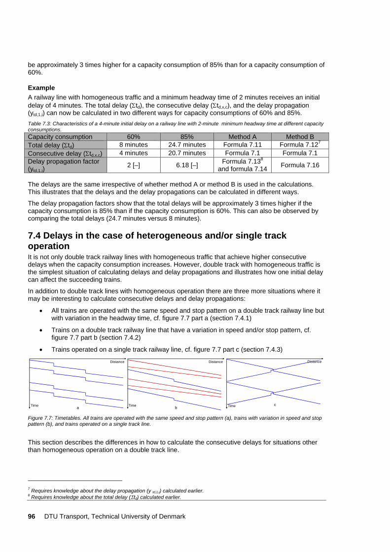
96 DTU Transport, Technical University of Denmark
be approximately 3 times higher for a capacity consumption of 85% than for a capacity consumption of 60%.
Example A railway line with homogeneous traffic and a minimum headway time of 2 minutes receives an initial delay of 4 minutes. The total delay (Σtd), the consecutive delay (Σtd,x,c), and the delay propagation (ytd,1,i) can now be calculated in two different ways for capacity consumptions of 60% and 85%. Table 7.3: Characteristics of a 4-minute initial delay on a railway line with 2-minute minimum headway time at different capacity consumptions. Capacity consumption 60% 85% Method A Method B Total delay (Σtd) 8 minutes 24.7 minutes Formula 7.11 Formula 7.127 Consecutive delay (Σtd,x,c) 4 minutes 20.7 minutes Formula 7.1 Formula 7.1 Delay propagation factor (ytd,1,i)
2 [–] 6.18 [–] Formula 7.138 and formula 7.14 Formula 7.16
The delays are the same irrespective of whether method A or method B is used in the calculations. This illustrates that the delays and the delay propagations can be calculated in different ways.
The delay propagation factors show that the total delays will be approximately 3 times higher if the capacity consumption is 85% than if the capacity consumption is 60%. This can also be observed by comparing the total delays (24.7 minutes versus 8 minutes).
7.4 Delays in the case of heterogeneous and/or single track operation It is not only double track railway lines with homogeneous traffic that achieve higher consecutive delays when the capacity consumption increases. However, double track with homogeneous traffic is the simplest situation of calculating delays and delay propagations and illustrates how one initial delay can affect the succeeding trains.
In addition to double track lines with homogeneous operation there are three more situations where it may be interesting to calculate consecutive delays and delay propagations:
• All trains are operated with the same speed and stop pattern on a double track railway line but with variation in the headway time, cf. figure 7.7 part a (section 7.4.1)
• Trains on a double track railway line that have a variation in speed and/or stop pattern, cf. figure 7.7 part b (section 7.4.2)
• Trains operated on a single track railway line, cf. figure 7.7 part c (section 7.4.3)
aTime
Distance
bTime
Distance
cTime
Distance
Figure 7.7: Timetables. All trains are operated with the same speed and stop pattern (a), trains with variation in speed and stop pattern (b), and trains operated on a single track line.
This section describes the differences in how to calculate the consecutive delays for situations other than homogeneous operation on a double track line.
7 Requires knowledge about the delay propagation (y td,1,i) calculated earlier. 8 Requires knowledge about the total delay (Σtd) calculated earlier.
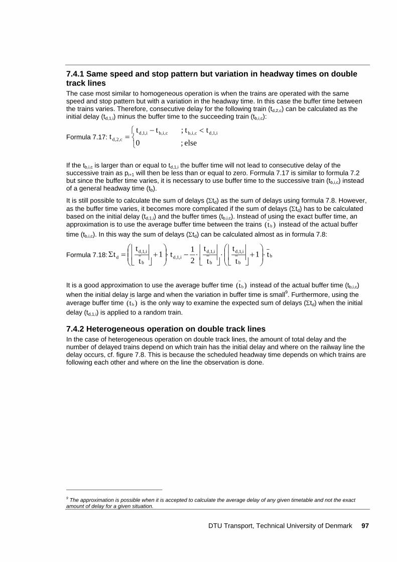
DTU Transport, Technical University of Denmark 97
7.4.1 Same speed and stop pattern but variation in headway times on double track lines The case most similar to homogeneous operation is when the trains are operated with the same speed and stop pattern but with a variation in the headway time. In this case the buffer time between the trains varies. Therefore, consecutive delay for the following train (td,2,c) can be calculated as the initial delay (td,1,i) minus the buffer time to the succeeding train (tb,i,c):
Formula 7.17: ⎩⎨⎧ <−
=else;0
tt;ttt i,1,dc,i,bc,i,bi,1,d
c,2,d
If the tb,i,c is larger than or equal to td,1,i the buffer time will not lead to consecutive delay of the successive train as pi+1 will then be less than or equal to zero. Formula 7.17 is similar to formula 7.2 but since the buffer time varies, it is necessary to use buffer time to the successive train (tb,i,c) instead of a general headway time (tb).
It is still possible to calculate the sum of delays (Σtd) as the sum of delays using formula 7.8. However, as the buffer time varies, it becomes more complicated if the sum of delays (Σtd) has to be calculated based on the initial delay (td,1,i) and the buffer times (tb,i,c). Instead of using the exact buffer time, an approximation is to use the average buffer time between the trains )t( b instead of the actual buffer time (tb,i,c). In this way the sum of delays (Σtd) can be calculated almost as in formula 7.8:
Formula 7.18: bb
i,1,d
b
i,1,di,1,d
b
i,1,dd t1
tt
tt
21t1
tt
t ⋅⎟⎟⎠
⎞⎜⎜⎝
⎛+⎥
⎦
⎥⎢⎣
⎢⋅⎥⎦
⎥⎢⎣
⎢⋅−⋅⎟⎟
⎠
⎞⎜⎜⎝
⎛+⎥
⎦
⎥⎢⎣
⎢=Σ
It is a good approximation to use the average buffer time )t( b instead of the actual buffer time (tb,i,c) when the initial delay is large and when the variation in buffer time is small9. Furthermore, using the average buffer time )t( b is the only way to examine the expected sum of delays (Σtd) when the initial delay (td,1,i) is applied to a random train.
7.4.2 Heterogeneous operation on double track lines In the case of heterogeneous operation on double track lines, the amount of total delay and the number of delayed trains depend on which train has the initial delay and where on the railway line the delay occurs, cf. figure 7.8. This is because the scheduled headway time depends on which trains are following each other and where on the line the observation is done.
9 The approximation is possible when it is accepted to calculate the average delay of any given timetable and not the exact amount of delay for a given situation.
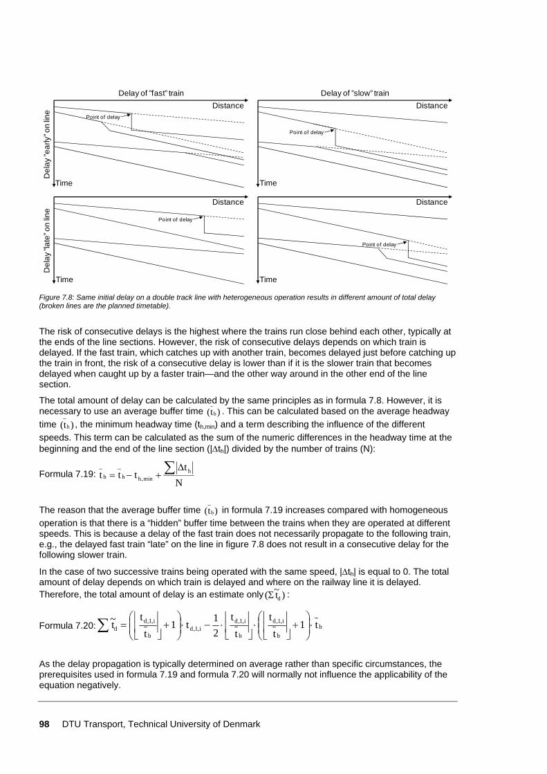
98 DTU Transport, Technical University of Denmark
Distance
Time
Point of delay
Distance
Time
Point of delay
Distance
Time
Point of delay
Distance
Time
Point of delay
Delay of ”fast” train Delay of ”slow” train
Del
ay ”e
arly
” on
line
Del
ay ”l
ate”
on
line
Figure 7.8: Same initial delay on a double track line with heterogeneous operation results in different amount of total delay (broken lines are the planned timetable).
The risk of consecutive delays is the highest where the trains run close behind each other, typically at the ends of the line sections. However, the risk of consecutive delays depends on which train is delayed. If the fast train, which catches up with another train, becomes delayed just before catching up the train in front, the risk of a consecutive delay is lower than if it is the slower train that becomes delayed when caught up by a faster train—and the other way around in the other end of the line section.
The total amount of delay can be calculated by the same principles as in formula 7.8. However, it is necessary to use an average buffer time )t( b . This can be calculated based on the average headway time )t( h , the minimum headway time (th,min) and a term describing the influence of the different speeds. This term can be calculated as the sum of the numeric differences in the headway time at the beginning and the end of the line section (|Δth|) divided by the number of trains (N):
Formula 7.19: N
tttt h
min,hh
_
b
_ ∑ Δ+−=
The reason that the average buffer time )t( b in formula 7.19 increases compared with homogeneous operation is that there is a “hidden” buffer time between the trains when they are operated at different speeds. This is because a delay of the fast train does not necessarily propagate to the following train, e.g., the delayed fast train “late” on the line in figure 7.8 does not result in a consecutive delay for the following slower train.
In the case of two successive trains being operated with the same speed, |Δth| is equal to 0. The total amount of delay depends on which train is delayed and where on the railway line it is delayed. Therefore, the total amount of delay is an estimate only )t~( dΣ :
Formula 7.20: bb
i,1,d
b
i,1,di,1,d
b
i,1,dd t1
tt
tt
21t1
tt
t~ ⋅⎟⎟⎠
⎞⎜⎜⎝
⎛+⎥
⎦
⎥⎢⎣
⎢⋅⎥⎦
⎥⎢⎣
⎢⋅−⋅⎟⎟
⎠
⎞⎜⎜⎝
⎛+⎥
⎦
⎥⎢⎣
⎢=∑
As the delay propagation is typically determined on average rather than specific circumstances, the prerequisites used in formula 7.19 and formula 7.20 will normally not influence the applicability of the equation negatively.
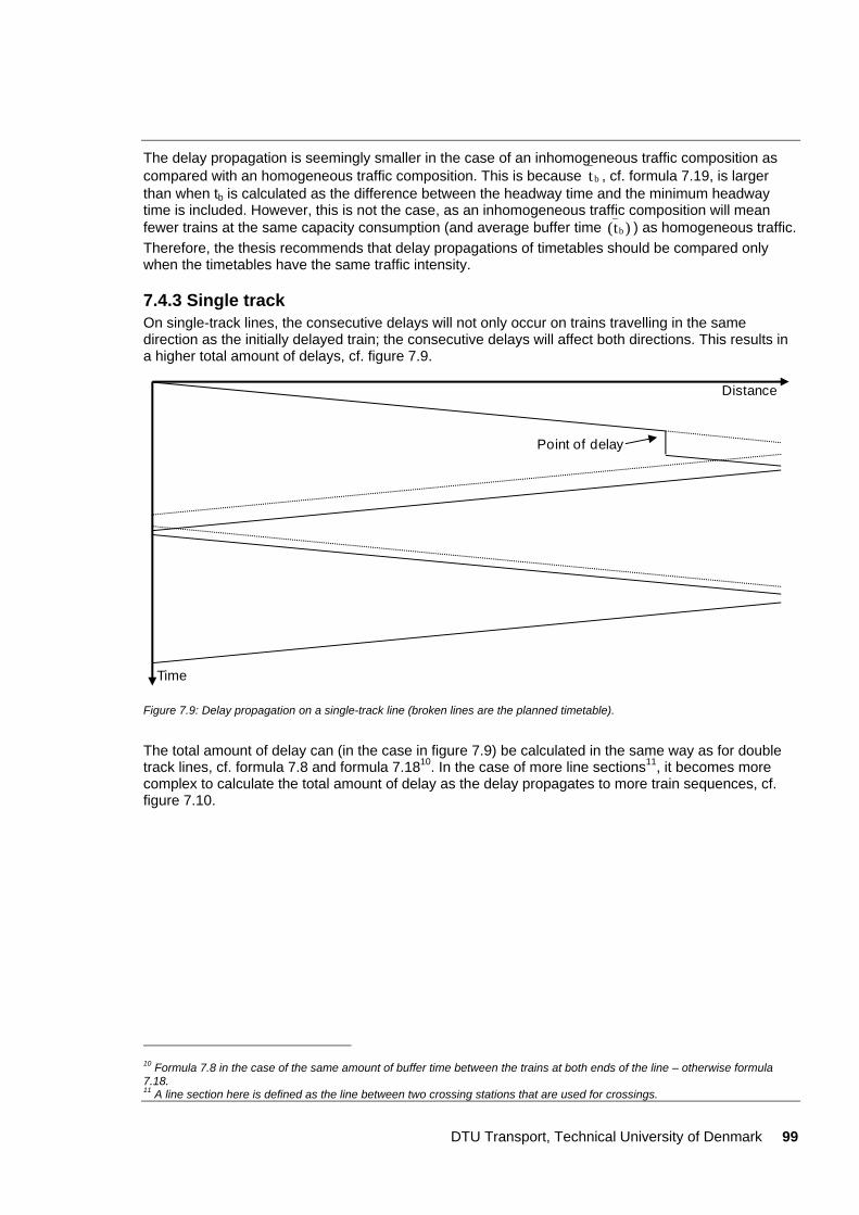
DTU Transport, Technical University of Denmark 99
The delay propagation is seemingly smaller in the case of an inhomogeneous traffic composition as compared with an homogeneous traffic composition. This is because bt , cf. formula 7.19, is larger than when tb is calculated as the difference between the headway time and the minimum headway time is included. However, this is not the case, as an inhomogeneous traffic composition will mean fewer trains at the same capacity consumption (and average buffer time )t( b ) as homogeneous traffic. Therefore, the thesis recommends that delay propagations of timetables should be compared only when the timetables have the same traffic intensity.
7.4.3 Single track On single-track lines, the consecutive delays will not only occur on trains travelling in the same direction as the initially delayed train; the consecutive delays will affect both directions. This results in a higher total amount of delays, cf. figure 7.9.
Time
Distance
Point of delay
Figure 7.9: Delay propagation on a single-track line (broken lines are the planned timetable).
The total amount of delay can (in the case in figure 7.9) be calculated in the same way as for double track lines, cf. formula 7.8 and formula 7.1810. In the case of more line sections11, it becomes more complex to calculate the total amount of delay as the delay propagates to more train sequences, cf. figure 7.10.
10 Formula 7.8 in the case of the same amount of buffer time between the trains at both ends of the line – otherwise formula 7.18. 11 A line section here is defined as the line between two crossing stations that are used for crossings.
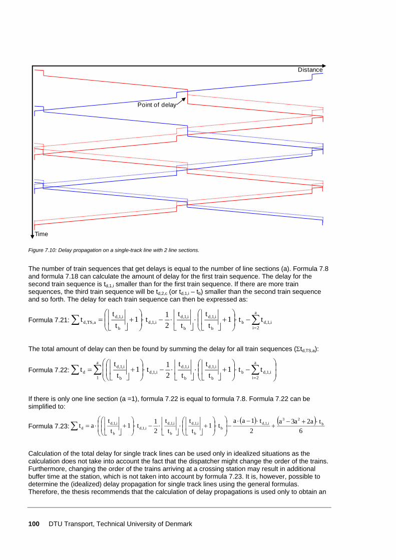
100 DTU Transport, Technical University of Denmark
Time
Distance
Point of delay
Figure 7.10: Delay propagation on a single-track line with 2 line sections.
The number of train sequences that get delays is equal to the number of line sections (a). Formula 7.8 and formula 7.18 can calculate the amount of delay for the first train sequence. The delay for the second train sequence is td,1,i smaller than for the first train sequence. If there are more train sequences, the third train sequence will be td,2,c (or td,1,i – tb) smaller than the second train sequence and so forth. The delay for each train sequence can then be expressed as:
Formula 7.21: ∑∑=
−⋅⎟⎟⎠
⎞⎜⎜⎝
⎛+⎥
⎦
⎥⎢⎣
⎢⋅⎥⎦
⎥⎢⎣
⎢⋅−⋅⎟⎟
⎠
⎞⎜⎜⎝
⎛+⎥
⎦
⎥⎢⎣
⎢=
a
2ii,1,db
b
i,1,d
b
i,1,di,1,d
b
i,1,da,TS,d tt1
tt
tt
21t1
tt
t
The total amount of delay can then be found by summing the delay for all train sequences (Σtd,TS,a):
Formula 7.22: ∑ ∑∑ ⎟⎟⎠
⎞⎜⎜⎝
⎛−⋅⎟⎟
⎠
⎞⎜⎜⎝
⎛+⎥
⎦
⎥⎢⎣
⎢⋅⎥⎦
⎥⎢⎣
⎢⋅−⋅⎟⎟
⎠
⎞⎜⎜⎝
⎛+⎥
⎦
⎥⎢⎣
⎢=
=
a
1
a
2ii,1,db
b
i,1,d
b
i,1,di,1,d
b
i,1,dd tt1
tt
tt
21t1
tt
t
If there is only one line section (a =1), formula 7.22 is equal to formula 7.8. Formula 7.22 can be simplified to:
Formula 7.23: ( ) ( )
6ta2a3a
2t1aa
t1t
tt
t21t1
tt
at b23
i,1,db
b
i,1,d
b
i,1,di,1,d
b
i,1,dd
⋅+−+
⋅−⋅−⎟
⎟⎠
⎞⎜⎜⎝
⎛⋅⎟⎟⎠
⎞⎜⎜⎝
⎛+⎥
⎦
⎥⎢⎣
⎢⋅⎥⎦
⎥⎢⎣
⎢⋅−⋅⎟⎟
⎠
⎞⎜⎜⎝
⎛+⎥
⎦
⎥⎢⎣
⎢⋅=∑
Calculation of the total delay for single track lines can be used only in idealized situations as the calculation does not take into account the fact that the dispatcher might change the order of the trains. Furthermore, changing the order of the trains arriving at a crossing station may result in additional buffer time at the station, which is not taken into account by formula 7.23. It is, however, possible to determine the (idealized) delay propagation for single track lines using the general formulas. Therefore, the thesis recommends that the calculation of delay propagations is used only to obtain an
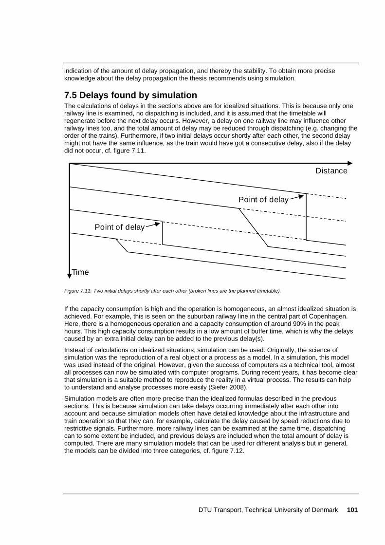
DTU Transport, Technical University of Denmark 101
indication of the amount of delay propagation, and thereby the stability. To obtain more precise knowledge about the delay propagation the thesis recommends using simulation.
7.5 Delays found by simulation The calculations of delays in the sections above are for idealized situations. This is because only one railway line is examined, no dispatching is included, and it is assumed that the timetable will regenerate before the next delay occurs. However, a delay on one railway line may influence other railway lines too, and the total amount of delay may be reduced through dispatching (e.g. changing the order of the trains). Furthermore, if two initial delays occur shortly after each other, the second delay might not have the same influence, as the train would have got a consecutive delay, also if the delay did not occur, cf. figure 7.11.
Time
Distance
Point of delay
Point of delay
Figure 7.11: Two initial delays shortly after each other (broken lines are the planned timetable).
If the capacity consumption is high and the operation is homogeneous, an almost idealized situation is achieved. For example, this is seen on the suburban railway line in the central part of Copenhagen. Here, there is a homogeneous operation and a capacity consumption of around 90% in the peak hours. This high capacity consumption results in a low amount of buffer time, which is why the delays caused by an extra initial delay can be added to the previous delay(s).
Instead of calculations on idealized situations, simulation can be used. Originally, the science of simulation was the reproduction of a real object or a process as a model. In a simulation, this model was used instead of the original. However, given the success of computers as a technical tool, almost all processes can now be simulated with computer programs. During recent years, it has become clear that simulation is a suitable method to reproduce the reality in a virtual process. The results can help to understand and analyse processes more easily (Siefer 2008).
Simulation models are often more precise than the idealized formulas described in the previous sections. This is because simulation can take delays occurring immediately after each other into account and because simulation models often have detailed knowledge about the infrastructure and train operation so that they can, for example, calculate the delay caused by speed reductions due to restrictive signals. Furthermore, more railway lines can be examined at the same time, dispatching can to some extent be included, and previous delays are included when the total amount of delay is computed. There are many simulation models that can be used for different analysis but in general, the models can be divided into three categories, cf. figure 7.12.

102 DTU Transport, Technical University of Denmark
Operational models
Tactical models
Strategic models
Planning horizon
Leve
l of d
etai
l
High
LowShort Long
Operation
Specialtimetables
Timetable
Plan of operation
Traffic forecasts
Figure 7.12: Different types of simulation models and their main types of analysis. Based on (Kaas 1998b).
For analysing delays and delay propagation, tactical (and/or operational) models can be used (e.g. RailSys (Siefer, Radtke 2005) and OpenTrack (Nash, Huerlimann 2004))12. These types of simulation model are generally built up in several steps. First, the infrastructure must be built up before constructing the timetable. Then, the delay distribution of the initial delays must be entered together with the rules for dispatching. Finally, the simulation can be run and the results can be evaluated, cf. figure 7.13. To ensure a stable and reproducible result, 50–200 simulations should be conducted (Siefer 2008)13.
The advantages of simulation models compared with the analytical models are the high accuracy and the possibility to test future changes in the infrastructure and the timetables for an entire network. Furthermore, simulation models can estimate the impact of the trains in the case of reduced speed and queuing, skip conditional stops, and change the order of the trains to reduce the amount of consecutive delays. However, simulation models also have their limits. Simulation models cannot dispatch the trains in the same way as does the dispatcher in real life, for example, it is difficult to set up rules when to cancel trains, leave out stops along the route, and turn around the trains before the line end station.
12 (Barber 2007) and (Koutsopoulos, Wang 2007) give an overview of different simulation tools. 13 (Radtke, Bendfeldt 2001) suggest 50–100 simulations.
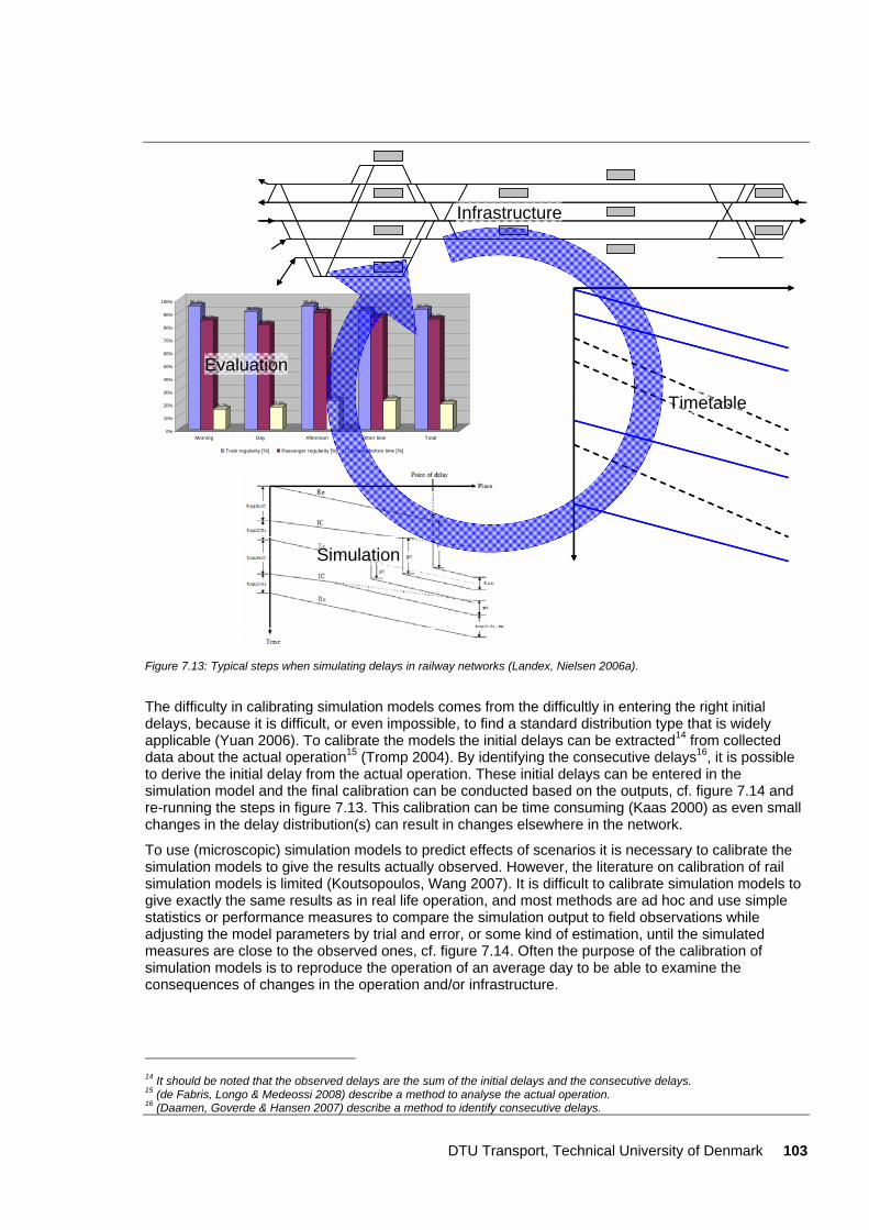
DTU Transport, Technical University of Denmark 103
95,4%
84,0%
15,7%
90,6%
80,5%
17,3%
95,4%90,3%
22,5%
91,4%86,8%
22,5%
92,7%
85,0%
19,6%
0%
10%
20%
30%
40%
50%
60%
70%
80%
90%
100%
Morning Day Afternoon Other time Total
Train regularity [%] Passenger regularity [%] Arrivals before time [%]
Infrastructure
Timetable
Evaluation
Simulation
Figure 7.13: Typical steps when simulating delays in railway networks (Landex, Nielsen 2006a).
The difficulty in calibrating simulation models comes from the difficultly in entering the right initial delays, because it is difficult, or even impossible, to find a standard distribution type that is widely applicable (Yuan 2006). To calibrate the models the initial delays can be extracted14 from collected data about the actual operation15 (Tromp 2004). By identifying the consecutive delays16, it is possible to derive the initial delay from the actual operation. These initial delays can be entered in the simulation model and the final calibration can be conducted based on the outputs, cf. figure 7.14 and re-running the steps in figure 7.13. This calibration can be time consuming (Kaas 2000) as even small changes in the delay distribution(s) can result in changes elsewhere in the network.
To use (microscopic) simulation models to predict effects of scenarios it is necessary to calibrate the simulation models to give the results actually observed. However, the literature on calibration of rail simulation models is limited (Koutsopoulos, Wang 2007). It is difficult to calibrate simulation models to give exactly the same results as in real life operation, and most methods are ad hoc and use simple statistics or performance measures to compare the simulation output to field observations while adjusting the model parameters by trial and error, or some kind of estimation, until the simulated measures are close to the observed ones, cf. figure 7.14. Often the purpose of the calibration of simulation models is to reproduce the operation of an average day to be able to examine the consequences of changes in the operation and/or infrastructure.
14 It should be noted that the observed delays are the sum of the initial delays and the consecutive delays. 15 (de Fabris, Longo & Medeossi 2008) describe a method to analyse the actual operation. 16 (Daamen, Goverde & Hansen 2007) describe a method to identify consecutive delays.
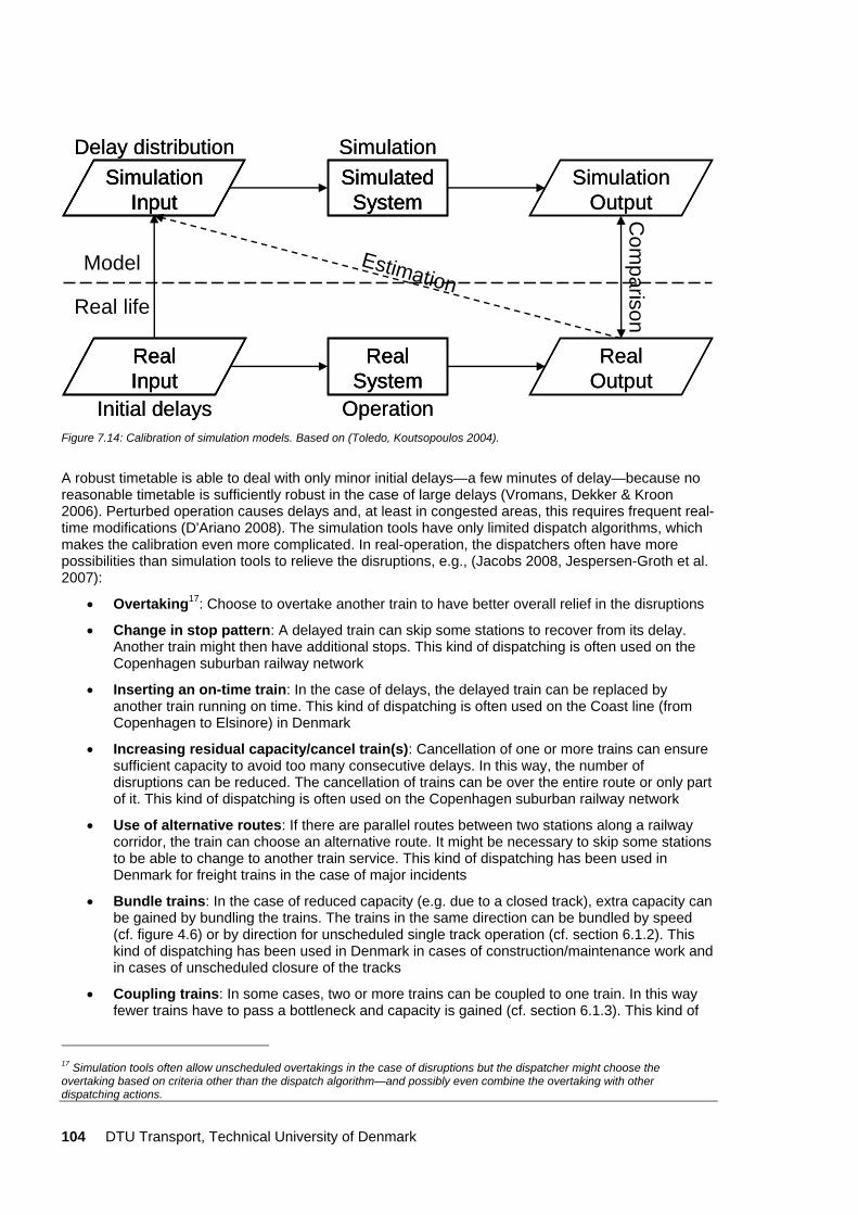
104 DTU Transport, Technical University of Denmark
SimulationOutput
SimulationOutput
RealOutputReal
Output
SimulatedSystem
SimulationSimulated
SystemSimulated
System
Simulation
RealSystem
Operation
RealSystem
RealSystem
Operation
Com
parison
RealInput
Initial delays
RealInputRealInput
Initial delays
SimulationInput
Delay distributionSimulation
InputSimulation
Input
Delay distribution
EstimationModel
Real life
Figure 7.14: Calibration of simulation models. Based on (Toledo, Koutsopoulos 2004).
A robust timetable is able to deal with only minor initial delays—a few minutes of delay—because no reasonable timetable is sufficiently robust in the case of large delays (Vromans, Dekker & Kroon 2006). Perturbed operation causes delays and, at least in congested areas, this requires frequent real-time modifications (D'Ariano 2008). The simulation tools have only limited dispatch algorithms, which makes the calibration even more complicated. In real-operation, the dispatchers often have more possibilities than simulation tools to relieve the disruptions, e.g., (Jacobs 2008, Jespersen-Groth et al. 2007):
• Overtaking17: Choose to overtake another train to have better overall relief in the disruptions
• Change in stop pattern: A delayed train can skip some stations to recover from its delay. Another train might then have additional stops. This kind of dispatching is often used on the Copenhagen suburban railway network
• Inserting an on-time train: In the case of delays, the delayed train can be replaced by another train running on time. This kind of dispatching is often used on the Coast line (from Copenhagen to Elsinore) in Denmark
• Increasing residual capacity/cancel train(s): Cancellation of one or more trains can ensure sufficient capacity to avoid too many consecutive delays. In this way, the number of disruptions can be reduced. The cancellation of trains can be over the entire route or only part of it. This kind of dispatching is often used on the Copenhagen suburban railway network
• Use of alternative routes: If there are parallel routes between two stations along a railway corridor, the train can choose an alternative route. It might be necessary to skip some stations to be able to change to another train service. This kind of dispatching has been used in Denmark for freight trains in the case of major incidents
• Bundle trains: In the case of reduced capacity (e.g. due to a closed track), extra capacity can be gained by bundling the trains. The trains in the same direction can be bundled by speed (cf. figure 4.6) or by direction for unscheduled single track operation (cf. section 6.1.2). This kind of dispatching has been used in Denmark in cases of construction/maintenance work and in cases of unscheduled closure of the tracks
• Coupling trains: In some cases, two or more trains can be coupled to one train. In this way fewer trains have to pass a bottleneck and capacity is gained (cf. section 6.1.3). This kind of
17 Simulation tools often allow unscheduled overtakings in the case of disruptions but the dispatcher might choose the overtaking based on criteria other than the dispatch algorithm—and possibly even combine the overtaking with other dispatching actions.
DTU Transport, Technical University of Denmark 105
dispatching has been used in Denmark in cases of construction/maintenance work and in cases of unscheduled closure of the tracks
Microscopic simulation models perform according to the rules entered. However, in the case of delays more passengers might want to use the same train, which might result in longer dwell times. This means that delayed trains generally have a higher risk of becoming even more delayed. However, if another train going in the same direction has overtaken the delayed train and is running immediately in front of the delayed train, the delayed train might have fewer passengers and thereby possible shorter dwell times, which is why the train may pick up time faster.
Although simulation models have disadvantages, they are more accurate than simple delay calculations. To overcome, or at least reduce, the disadvantages of simulation models, the results are often compared relatively to each other. In this way, it is possible to examine the relative differences for different projects and choose the best alternative.
Microscopic simulation models are powerful, but they require extensive work to enter the detailed infrastructure topology, train characteristics, signal locations and timetables. Furthermore, these models require more computing time compared with simpler models, which is why it might be tempting to use these simpler macroscopic or operation research models18. Although these models are suitable for evaluating the overall stability of timetables of interconnected lines, they cannot be used to estimate the distributions of consecutive delays and the punctuality level of the scheduled trains, as they are generally based on a deterministic modelling approach (Yuan 2006). Nevertheless, the simpler models give an indication about the delay(s) that might be satisfactory—at least in a screening process with several alternatives. To achieve better simulation results from simulation models, further research and development is needed, especially within dispatch algorithms.
7.6 Summary Delays on railways can be divided into initial delays and consecutive delays. The amount of consecutive delays can be estimated based on the initial delay, the headway time, and the minimum headway time. The higher the capacity consumption on railway lines the higher the risk of consecutive delays.
Consecutive delays can be estimated mathematically for both double- and single-track railway lines. However, the estimated delays are often for idealized situations only, as delays can propagate from railway line to railway line and two initial delays occurring immediately after each other will most often result in less consecutive delays than if the initial delays occurred at longer time intervals.
To have a more accurate estimation of delays, the thesis recommends simulation models. The simulation models can calculate the delays for an entire network and also take the time interval between the initial delays into account. Although simulation models are the most accurate method to estimate delays, the models could be more accurate as they could use more realistic dispatching strategies.
18 Microscopic models require more detailed data than do the simpler models. In some countries these data are difficult to procure, but in Denmark there is open access to the data.

106 DTU Transport, Technical University of Denmark
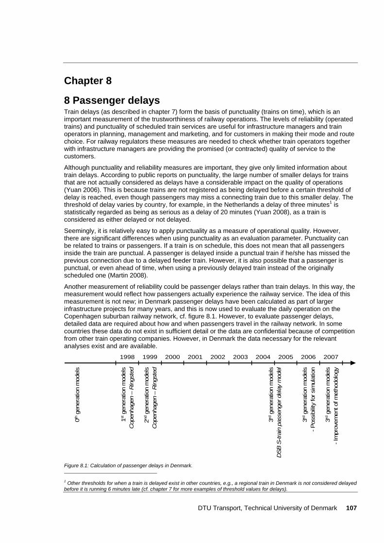
DTU Transport, Technical University of Denmark 107
Chapter 8
8 Passenger delays Train delays (as described in chapter 7) form the basis of punctuality (trains on time), which is an important measurement of the trustworthiness of railway operations. The levels of reliability (operated trains) and punctuality of scheduled train services are useful for infrastructure managers and train operators in planning, management and marketing, and for customers in making their mode and route choice. For railway regulators these measures are needed to check whether train operators together with infrastructure managers are providing the promised (or contracted) quality of service to the customers.
Although punctuality and reliability measures are important, they give only limited information about train delays. According to public reports on punctuality, the large number of smaller delays for trains that are not actually considered as delays have a considerable impact on the quality of operations (Yuan 2006). This is because trains are not registered as being delayed before a certain threshold of delay is reached, even though passengers may miss a connecting train due to this smaller delay. The threshold of delay varies by country, for example, in the Netherlands a delay of three minutes1 is statistically regarded as being as serious as a delay of 20 minutes (Yuan 2008), as a train is considered as either delayed or not delayed.
Seemingly, it is relatively easy to apply punctuality as a measure of operational quality. However, there are significant differences when using punctuality as an evaluation parameter. Punctuality can be related to trains or passengers. If a train is on schedule, this does not mean that all passengers inside the train are punctual. A passenger is delayed inside a punctual train if he/she has missed the previous connection due to a delayed feeder train. However, it is also possible that a passenger is punctual, or even ahead of time, when using a previously delayed train instead of the originally scheduled one (Martin 2008).
Another measurement of reliability could be passenger delays rather than train delays. In this way, the measurement would reflect how passengers actually experience the railway service. The idea of this measurement is not new; in Denmark passenger delays have been calculated as part of larger infrastructure projects for many years, and this is now used to evaluate the daily operation on the Copenhagen suburban railway network, cf. figure 8.1. However, to evaluate passenger delays, detailed data are required about how and when passengers travel in the railway network. In some countries these data do not exist in sufficient detail or the data are confidential because of competition from other train operating companies. However, in Denmark the data necessary for the relevant analyses exist and are available.
0thge
nera
tion
mod
els
20061998
1stge
nera
tion
mod
els
Cop
enha
gen
–R
ings
ted
2ndge
nera
tion
mod
els
Cop
enha
gen
–R
ings
ted
3rdge
nera
tion
mod
els
DS
B S
-trai
n pa
ssen
ger d
elay
mod
el
3rdge
nera
tion
mod
els
-Pos
sibi
lity
for s
imul
atio
n
20031999 2000 2001 2002 2004 2005 2007
3rdge
nera
tion
mod
els
-Im
prov
emen
t of m
etho
dolo
gy
Figure 8.1: Calculation of passenger delays in Denmark. 1 Other thresholds for when a train is delayed exist in other countries, e.g., a regional train in Denmark is not considered delayed before it is running 6 minutes late (cf. chapter 7 for more examples of threshold values for delays).
108 DTU Transport, Technical University of Denmark
As calculation of passenger delays differs greatly from the previous topics of this thesis, a literature review is given in section 8.1. This is followed by different methods to calculate passenger delays (section 8.2), and how the newest 3rd generation of passenger delay models works in practice (section 8.3), and results from real life operation (section 8.4). In section 8.5, 3rd generation models are combined with standard micro-simulation software, i.e., RailSys, to estimate the future passenger delay. Section 8.6 describes how the 3rd generation model combined with micro-simulation can be used in the planning process to improve the later operation. Lastly, section 8.7 gives an overview of how the 3rd generation model can be improved before section 8.8 summarizes the chapter.
This chapter is partly based on (Nielsen, Landex & Frederiksen 2008). However, the 3rd generation passenger delay model suggested in (Nielsen, Landex & Frederiksen 2008) has been updated to a newer version. Since the topic of this chapter is technically different from the previous chapters, references are made to the definitions in Appendix 1.
8.1 Literature review Research in how passengers perceive their value of time indicates that delays and variability of travel time is perceived worse than the expected travel time, i.e., the value of time of delay is higher (Bates et al. 2001, Noland, Polak 2002).
Although delays have great importance for people’s valuation of public transport, evaluation and forecasts of punctuality and reliability of railway systems, where they have been done at all, have been computed for trains, not for passengers. Furthermore, when passenger delays have been calculated, the underlying models have not explicitly considered how passengers react to the delays they experience en route when they are travelling. Passenger delays, however, differ from train delays due to the following reasons:
• The number of passengers per train varies. In periods with many passengers per train, there is a high risk of delays2. Therefore, trains in the peak hours are more likely to be delayed than trains with fewer passengers outside the rush hours. Since the capacity consumption is often higher in the peak hours (due to more and/or longer trains), there is a higher risk of consecutive delays. As most passengers travel during the peak hours, train delay measurements tend to underestimate the delays experienced by the passengers.
• Passenger transfers between train lines. Providing the next train is reached, passengers may consider only the delay of the delayed train as a problem. However, if the connection is missed, the delay may be much larger than only the delay of the arriving train (Bates et al. 2001). Some passengers may even obtain a better connection, if a prior and/or more convenient train connection is delayed, whereby the passenger can board the delayed train and reach the final destination before planned.
• The same railway line may be served by many train services. Passengers on short trips may not experience a delay if they can take another train at the planned time leading to the same destination as the planned rail service.
Until 2005, the Copenhagen Suburban Rail company (DSB S-tog) measured only train reliability (operated trains) and punctuality (trains on time). However, it later became desirable to also measure passenger delays. This is defined as the delays experienced by passengers when arriving at their destination compared with the arrival time according to the planned timetable. The purpose of quantifying the passenger delays was two-fold:
1. To be able to deliver more detailed reports on passenger delays to the Ministry of Transport.
2. To provide a better basis for planning in the company. The latter including designing timetables and planning the use of rolling stock with respect to passenger flows.
2 Regular fixed interval timetable assumed.
DTU Transport, Technical University of Denmark 109
To quantify the passenger delays, the schedule-based route choice model3 presented in (Nielsen 2004) was further developed to model passenger delays for the Copenhagen Suburban Rail company (Nielsen, Landex & Frederiksen 2008).
Little research has been done in modelling delays in schedule-based route choice models (Nielsen, Landex & Frederiksen 2008). In general, the majority of schedule-based route choice models assume that the timetable is deterministic, i.e., with no delays (refer to the classification in table 8.1). The route choice models are also often deterministic, i.e., they assume a deterministic choice behaviour of the passengers, hence the name deterministic route choice models. However, during the last 5–10 years stochastic schedule-based models have emerged (refer to the review in (Nuzzolo, Crisalli 2004)). Whilst the earlier stochastic choice models applied the logit model4, the newer models account for overlapping routes. Examples are the approach applied in (Friedrich, Wekeck 2004), path size logit (Hoogendoorn-Lanser 2005) or Probit (Nielsen 2004). An additional feature is the use of random coefficients such as in (Nielsen, Jovicic 1999). (Mabit, Nielsen 2006) developed this further to take correlation of taste preferences into account. Table 8.1: Classification of schedule-based assignment problems (Nielsen, Landex & Frederiksen 2008).
Delay considerations
Deterministic route choice model Stochastic route choice model
No capacity restrictions
Within coach capacity
restrictions
No capacity restrictions
Within coach capacity
restrictions
Deterministic timetable
Majority of schedule-based
assignment methods
Some applications
Logit Path Size Logit
Probit Mixed Probit
Few applications based on
Stochastic User Equilibrium
Timetable with delays
Full a priori knowledge
In principle as the deterministic methods, but run on the delayed timetable, e.g. principle 4 in (Hickmann, Bernstein 1997)
Knowledge on the delay distribution
– – (Nuzzolo, Russo & Crisalli 2001)
(Nielsen, Hansen & Daly 2001)
On-route decisions
Principle 3 in (Hickmann,
Bernstein 1997) –
(Nuzzolo, Crisalli 2004), this
chapter and (Nielsen, Landex
& Frederiksen 2008)
–
A few models also consider the within coach capacity restrictions, such as having a seat or not (Nielsen, Hansen & Daly 2001) or overloaded coaches (rejection of passengers who wish to board). A review of the literature is given in (Nuzzolo, Crisalli 2004). Rejections of passengers may be more relevant for urban bus transport, long distance rail transport, air transport or freight transport in schedule-based networks than for suburban railway lines where passengers are seldom rejected. However, an important point is that capacity problems may be more relevant in networks with delays due to arrival processes of passengers. If passengers’ arrival is partly uniformly distributed, more are expected to board the delayed services. If passengers from one service miss their connection, the number of transferring passengers may be doubled when the next connection arrives.
Concerning route choice modelling of networks with delays, a few prior models have been identified. Whilst (Nuzzolo, Crisalli 2004) provide a classification scheme for irregular services (cf. table 5.1 in (Nuzzolo, Crisalli 2004)), only few references are given, mainly to (Hickmann, Bernstein 1997). In
3 A model that based on the exact timetable, an OD-matrix, and the passengers’ preferences for travel time, transfer time, waiting time etc. calculates the route of the passengers and assigns passengers to the route network. 4 A discrete choice model that is based on the assumption that the error terms are independent and identically gumbel distributed.
110 DTU Transport, Technical University of Denmark
addition to this, (Bates et al. 2001) define some principles for the problems of unreliability and interchange journeys.
Earlier models (1st generation delay models, cf. section 8.2.2) assumed full knowledge of present and future delays. An example is the fourth path choice principle in (Hickmann, Bernstein 1997). In principle, this is similar to operating a deterministic timetable based model on the delayed network and then comparing this with the same model run on the non-delayed network. This is a “pseudo” delay model, as the model has no assumptions regarding passenger behaviour or on-trip re-routing if trains are delayed5. The route choice principles can therefore, in principle, be identical to the deterministic schedule-based methods.
An improvement of the 1st generation model was applied in (Ildenborg-Hansen 2006) where passengers are assumed to arrive at the departing station according to their a priori choices. But from then on full knowledge is assumed. (Landex, Nielsen 2006c) classify this approach as a 1½ generation model. (Nuzzolo, Crisalli 2004) also assume a re-consideration at the stop (here in a bus-network application), given knowledge from a passenger information system.
(Nuzzolo, Russo & Crisalli 2001) proposed a method to simulate transit irregularity and to apply a schedule-based route choice model on the irregular timetables. The approach may be considered somewhat similar to that of (Nielsen, Hansen & Daly 2001), i.e.. that passengers are implicitly assumed to know the delay distribution. In (Landex, Nielsen 2006c) this is classified as a 2nd generation model, as passengers are assumed to know the delay distribution a priori and then to choose route pre-trip according to the expected delay distribution.
(Nielsen, Landex & Frederiksen 2008) argue that passengers do not have full (a priori) knowledge of future delays in a public transport network. Therefore, passengers are most likely expected to reconsider their route choices along the route, if and when delays occur. However, passengers may not realize the delays instantly; instead, they may react within a certain threshold. No such schedule-based model has earlier been developed (Nielsen, Landex & Frederiksen 2008), while the benchmark (or “pessimistic” principle) is similar to the second route choice principle in (Hickmann, Bernstein 1997), “passengers use the time-dependent static path choice model to determine their boarding strategies”. This may be constrained due to transfers that are no longer possible (cf. principle 3 in (Hickmann, Bernstein 1997)).
According to (Nielsen, Landex & Frederiksen 2008), the realistic choice of the passengers is somewhere between the results of the following model principles:
• A pure pre-trip decision of the route based on the planned timetable and without changes of the planned route except if the pre-trip decisions are not possible
• An optimistic optimal choice of route based on full knowledge of all (future) delays
8.2 Methods to calculate passenger delays Several methods have been applied to calculate rail passenger delays. The majority of these do not include schedule-based route choice models, in the following classified as 0th generation models. Some methods are simple and straightforward to implement, but they are also simplified and inaccurate; other methods are more precise. The simplest methods (0th generation) are not reported in the international literature as they have been developed and used by railway companies, which is why the description of these is based on interviews with railway companies. Although the 0th generation methods are simple and inaccurate, these models form the basis for the later 1st, 1½, 2nd and 3rd generation passenger delay models.
8.2.1 Traditional calculation – 0th generation Common for all 0th generation models is that they do not model changes in passengers’ route choices. As passenger delays depend on the route choice of the passengers, these models are labelled “0th generation” as they are the generation before the first implementation of schedule-based models for 5 Passengers in the train will seldom change their route choice, whereas passengers waiting at the station are more likely to change their route choice and board the first train in their direction.
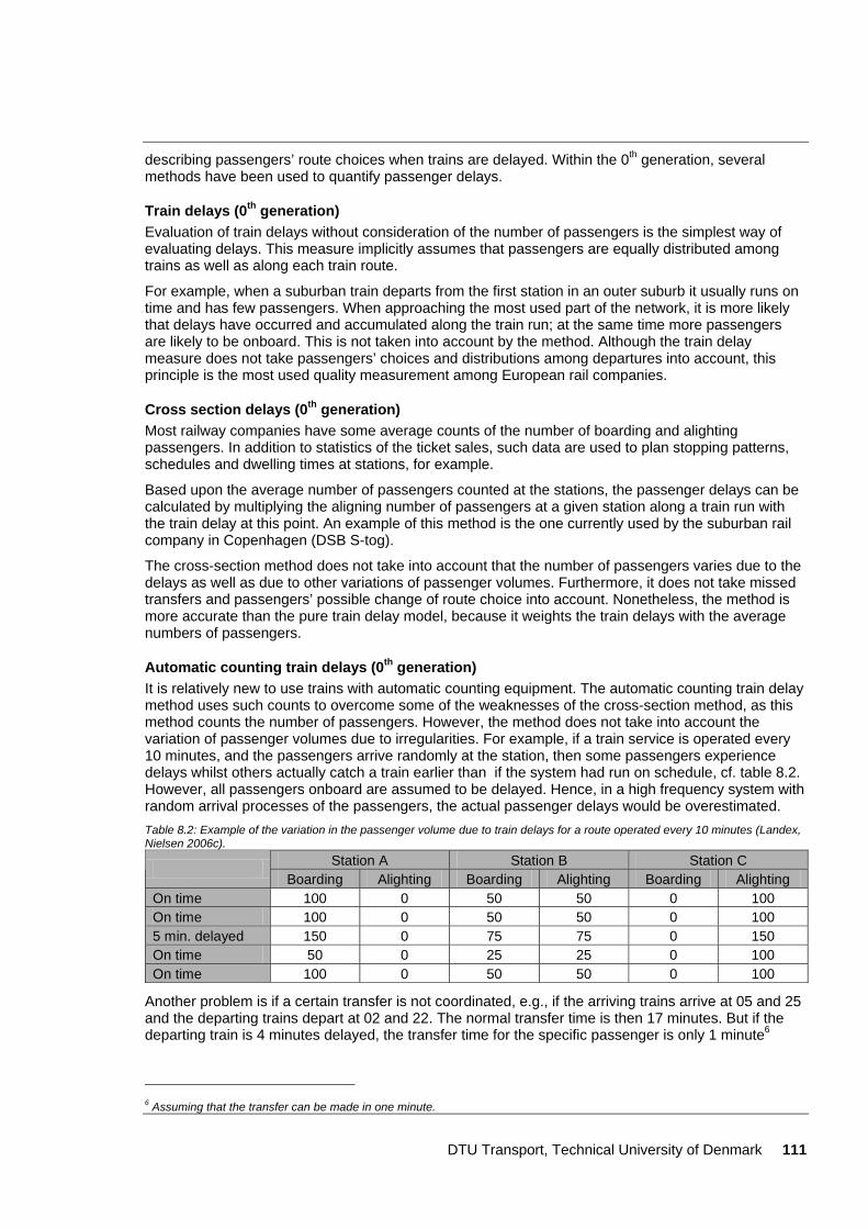
DTU Transport, Technical University of Denmark 111
describing passengers’ route choices when trains are delayed. Within the 0th generation, several methods have been used to quantify passenger delays.
Train delays (0th generation) Evaluation of train delays without consideration of the number of passengers is the simplest way of evaluating delays. This measure implicitly assumes that passengers are equally distributed among trains as well as along each train route.
For example, when a suburban train departs from the first station in an outer suburb it usually runs on time and has few passengers. When approaching the most used part of the network, it is more likely that delays have occurred and accumulated along the train run; at the same time more passengers are likely to be onboard. This is not taken into account by the method. Although the train delay measure does not take passengers’ choices and distributions among departures into account, this principle is the most used quality measurement among European rail companies.
Cross section delays (0th generation) Most railway companies have some average counts of the number of boarding and alighting passengers. In addition to statistics of the ticket sales, such data are used to plan stopping patterns, schedules and dwelling times at stations, for example.
Based upon the average number of passengers counted at the stations, the passenger delays can be calculated by multiplying the aligning number of passengers at a given station along a train run with the train delay at this point. An example of this method is the one currently used by the suburban rail company in Copenhagen (DSB S-tog).
The cross-section method does not take into account that the number of passengers varies due to the delays as well as due to other variations of passenger volumes. Furthermore, it does not take missed transfers and passengers’ possible change of route choice into account. Nonetheless, the method is more accurate than the pure train delay model, because it weights the train delays with the average numbers of passengers.
Automatic counting train delays (0th generation) It is relatively new to use trains with automatic counting equipment. The automatic counting train delay method uses such counts to overcome some of the weaknesses of the cross-section method, as this method counts the number of passengers. However, the method does not take into account the variation of passenger volumes due to irregularities. For example, if a train service is operated every 10 minutes, and the passengers arrive randomly at the station, then some passengers experience delays whilst others actually catch a train earlier than if the system had run on schedule, cf. table 8.2. However, all passengers onboard are assumed to be delayed. Hence, in a high frequency system with random arrival processes of the passengers, the actual passenger delays would be overestimated. Table 8.2: Example of the variation in the passenger volume due to train delays for a route operated every 10 minutes (Landex, Nielsen 2006c).
Station A Station B Station C Boarding Alighting Boarding Alighting Boarding Alighting
On time 100 0 50 50 0 100 On time 100 0 50 50 0 100 5 min. delayed 150 0 75 75 0 150 On time 50 0 25 25 0 100 On time 100 0 50 50 0 100
Another problem is if a certain transfer is not coordinated, e.g., if the arriving trains arrive at 05 and 25 and the departing trains depart at 02 and 22. The normal transfer time is then 17 minutes. But if the departing train is 4 minutes delayed, the transfer time for the specific passenger is only 1 minute6
6 Assuming that the transfer can be made in one minute.
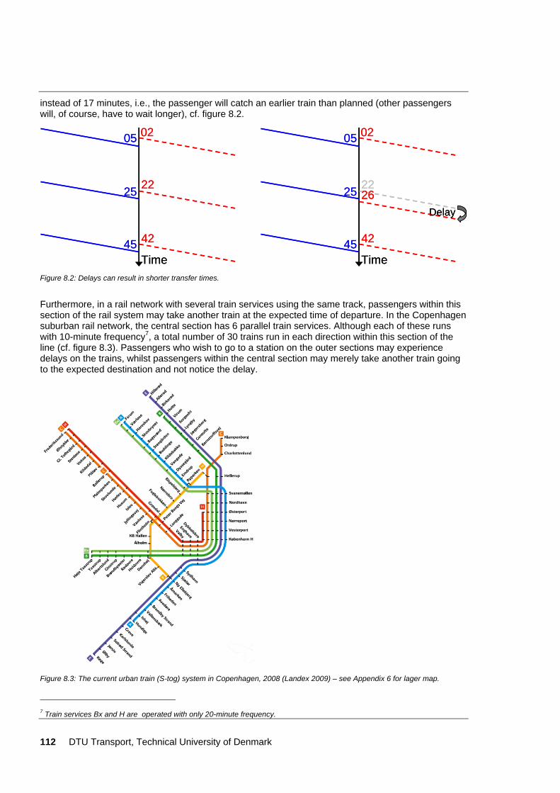
112 DTU Transport, Technical University of Denmark
instead of 17 minutes, i.e., the passenger will catch an earlier train than planned (other passengers will, of course, have to wait longer), cf. figure 8.2.
05
25
45
02
22
42
Time
05
25
45
02
22
42
Time
05
25
45
02
22
42
Time
26Delay
05
25
45
02
22
42
Time
26Delay
Figure 8.2: Delays can result in shorter transfer times.
Furthermore, in a rail network with several train services using the same track, passengers within this section of the rail system may take another train at the expected time of departure. In the Copenhagen suburban rail network, the central section has 6 parallel train services. Although each of these runs with 10-minute frequency7, a total number of 30 trains run in each direction within this section of the line (cf. figure 8.3). Passengers who wish to go to a station on the outer sections may experience delays on the trains, whilst passengers within the central section may merely take another train going to the expected destination and not notice the delay.
Figure 8.3: The current urban train (S-tog) system in Copenhagen, 2008 (Landex 2009) – see Appendix 6 for lager map.
7 Train services Bx and H are operated with only 20-minute frequency.

DTU Transport, Technical University of Denmark 113
8.2.2 Optimal route choice – 1st generation The core idea of the 1st generation passenger delay models is that the passenger delays are modelled by assigning a time-space trip matrix based upon the realized timetable by an optimal route choice model8. The optimality is with regard to the delayed timetable, which is assumed to be known in advance by the passengers. The route choice criteria itself can still be stochastic by having stochastic parameters of the passengers’ route choices in, e.g., a logit or Probit model. The result of the route choice is compared to a calculation where passengers are assigned according to the planned timetable (the announced official timetable), cf. figure 8.4.
Calculation of time spent in the system by use of a route choice model used on
the planned timetable
Difference in time⇓
Delay
Calculation of time spent in the system by use of a route choice model used on
the realized timetable
Figure 8.4: The core principle of 1st generation passenger delay models.
The advantage of this 1st generation passenger delay model is that it takes the passengers’ route choices into account (in contrast to the 0th generation methods), whereby the model is more precise. Moreover, the model can be applied by simply running a standard schedule-based route choice model on the delayed timetable. Another advantage of the 1st generation model is that it is the delay of the entire trip (including transfers) that is examined.
The disadvantage is that passengers are implicitly assumed to know both the current and the future delays in advance as the route choice model is used to calculate the time spent in the system with the realized timetable. Therefore, the passengers are assumed to plan according to the realized timetable. This underestimates the passenger delays compared with real travel, where some, or most, of the passengers first realize the delays during their trip. An example of the underestimation of delays is a passenger travelling from A to C (cf. figure 8.5), where the direct train from A to C comes to an unscheduled stop (e.g., due to signal dysfunction or a fault on the train). As the passenger (in the model) knows that the direct train will be delayed before it actually happens, the passenger will take the detour via B instead—a detour that is normally not considered an option due to the extra transfer and the extra travel time9.
A B
C Figure 8.5: Stylized route network for a simple railway network.
8 In an optimal route choice model it is assumed that the passengers know the exact timetable for the entire network including all (future) delays of the trains. 9 This kind of detour can occur both at suburban and long distance railway networks when the additional time for the detour is small and/or the delays are large.
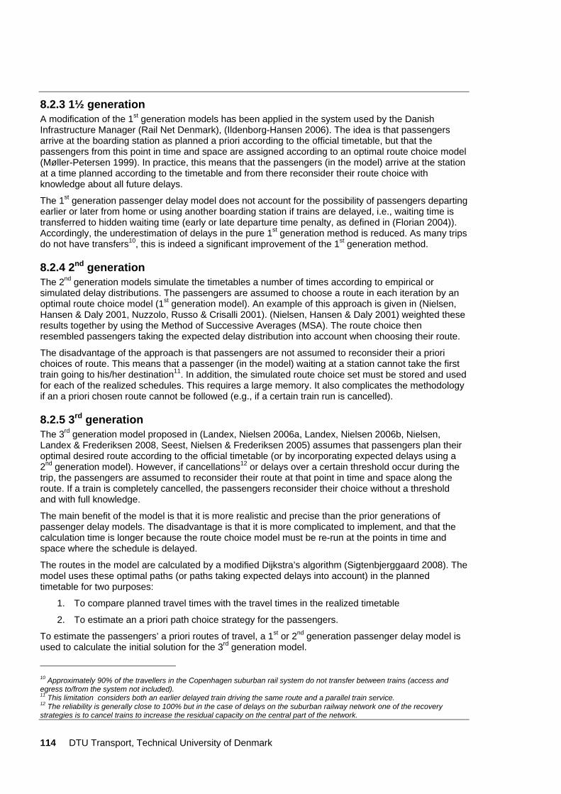
114 DTU Transport, Technical University of Denmark
8.2.3 1½ generation A modification of the 1st generation models has been applied in the system used by the Danish Infrastructure Manager (Rail Net Denmark), (Ildenborg-Hansen 2006). The idea is that passengers arrive at the boarding station as planned a priori according to the official timetable, but that the passengers from this point in time and space are assigned according to an optimal route choice model (Møller-Petersen 1999). In practice, this means that the passengers (in the model) arrive at the station at a time planned according to the timetable and from there reconsider their route choice with knowledge about all future delays.
The 1st generation passenger delay model does not account for the possibility of passengers departing earlier or later from home or using another boarding station if trains are delayed, i.e., waiting time is transferred to hidden waiting time (early or late departure time penalty, as defined in (Florian 2004)). Accordingly, the underestimation of delays in the pure 1st generation method is reduced. As many trips do not have transfers10, this is indeed a significant improvement of the 1st generation method.
8.2.4 2nd generation The 2nd generation models simulate the timetables a number of times according to empirical or simulated delay distributions. The passengers are assumed to choose a route in each iteration by an optimal route choice model (1st generation model). An example of this approach is given in (Nielsen, Hansen & Daly 2001, Nuzzolo, Russo & Crisalli 2001). (Nielsen, Hansen & Daly 2001) weighted these results together by using the Method of Successive Averages (MSA). The route choice then resembled passengers taking the expected delay distribution into account when choosing their route.
The disadvantage of the approach is that passengers are not assumed to reconsider their a priori choices of route. This means that a passenger (in the model) waiting at a station cannot take the first train going to his/her destination11. In addition, the simulated route choice set must be stored and used for each of the realized schedules. This requires a large memory. It also complicates the methodology if an a priori chosen route cannot be followed (e.g., if a certain train run is cancelled).
8.2.5 3rd generation The 3rd generation model proposed in (Landex, Nielsen 2006a, Landex, Nielsen 2006b, Nielsen, Landex & Frederiksen 2008, Seest, Nielsen & Frederiksen 2005) assumes that passengers plan their optimal desired route according to the official timetable (or by incorporating expected delays using a 2nd generation model). However, if cancellations12 or delays over a certain threshold occur during the trip, the passengers are assumed to reconsider their route at that point in time and space along the route. If a train is completely cancelled, the passengers reconsider their choice without a threshold and with full knowledge.
The main benefit of the model is that it is more realistic and precise than the prior generations of passenger delay models. The disadvantage is that it is more complicated to implement, and that the calculation time is longer because the route choice model must be re-run at the points in time and space where the schedule is delayed.
The routes in the model are calculated by a modified Dijkstra’s algorithm (Sigtenbjerggaard 2008). The model uses these optimal paths (or paths taking expected delays into account) in the planned timetable for two purposes:
1. To compare planned travel times with the travel times in the realized timetable
2. To estimate an a priori path choice strategy for the passengers.
To estimate the passengers’ a priori routes of travel, a 1st or 2nd generation passenger delay model is used to calculate the initial solution for the 3rd generation model.
10 Approximately 90% of the travellers in the Copenhagen suburban rail system do not transfer between trains (access and egress to/from the system not included). 11 This limitation considers both an earlier delayed train driving the same route and a parallel train service. 12 The reliability is generally close to 100% but in the case of delays on the suburban railway network one of the recovery strategies is to cancel trains to increase the residual capacity on the central part of the network.
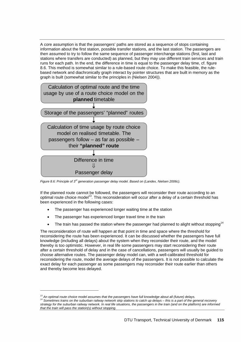
DTU Transport, Technical University of Denmark 115
A core assumption is that the passengers’ paths are stored as a sequence of stops containing information about the first station, possible transfer stations, and the last station. The passengers are then assumed to try to follow the same sequence of passenger interchange stations (first, last and stations where transfers are conducted) as planned, but they may use different train services and train runs for each path. In the end, the difference in time is equal to the passenger delay time, cf. figure 8.6. This method is somewhat similar to a rule-based route choice. To make this feasible, the rule-based network and diachronically graph interact by pointer structures that are built in memory as the graph is built (somewhat similar to the principles in (Nielsen 2004)).
Calculation of optimal route and the time usage by use of a route choice model on the
planned timetable
Calculation of time usage by route choice model on realised timetable. The
passengers follow – as far as possible –their “planned” route
Difference in time⇓
Passenger delay
Storage of the passengers’ “planned” routes
Figure 8.6: Principle of 3rd generation passenger delay model. Based on (Landex, Nielsen 2006c).
If the planned route cannot be followed, the passengers will reconsider their route according to an optimal route choice model13. This reconsideration will occur after a delay of a certain threshold has been experienced in the following cases:
• The passenger has experienced longer waiting time at the station
• The passenger has experienced longer travel time in the train
• The train has passed the station where the passenger had planned to alight without stopping14
The reconsideration of route will happen at that point in time and space where the threshold for reconsidering the route has been experienced. It can be discussed whether the passengers have full knowledge (including all delays) about the system when they reconsider their route, and the model thereby is too optimistic. However, in real life some passengers may start reconsidering their route after a certain threshold of delay and in the case of cancellations, passengers will usually be guided to choose alternative routes. The passenger delay model can, with a well-calibrated threshold for reconsidering the route, model the average delays of the passengers. It is not possible to calculate the exact delay for each passenger as some passengers may reconsider their route earlier than others and thereby become less delayed.
13 An optimal route choice model assumes that the passengers have full knowledge about all (future) delays. 14 Sometimes trains on the suburban railway network skip stations to catch up delays – this is a part of the general recovery strategy for the suburban railway network. In real life situations, the passengers in the train (and on the platform) are informed that the train will pass the station(s) without stopping.
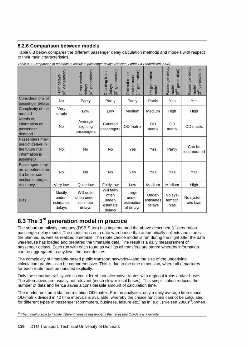
116 DTU Transport, Technical University of Denmark
8.2.6 Comparison between models Table 8.3 below compares the different passenger delay calculation methods and models with respect to their main characteristics. Table 8.3: Comparison of methods to calculate passenger delays (Nielsen, Landex & Frederiksen 2008).
Trai
n de
lays
(0
th g
ener
atio
n)
Cro
ss s
ectio
n de
lays
(0
th g
ener
atio
n)
Cou
ntin
g tra
in
dela
ys
(0th g
ener
atio
n)
Opt
imal
rout
e ch
oice
mod
el
(1st g
ener
atio
n)
1½ g
ener
atio
n m
odel
Pass
enge
r del
ay
mod
el
(2nd
gen
erat
ion)
Pass
enge
r del
ay
mod
el
(3rd
gen
erat
ion)
Considerations of passenger delays No Partly Partly Partly Partly Yes Yes
Complexity of the method
Very simple Low Low Medium Medium High High
Needs of information on passenger demand
No Average alighting
passengers
Counted passengers OD matrix OD
matrix OD
matrix OD matrix
Passengers may predict delays in the future (full information is assumed)
No No No Yes Yes Partly Can be incorporated
Passengers may arrive before time if a better con-nection emerges
No No No Yes Yes Yes Yes
Accuracy Very low Quite low Fairly low Low Medium Medium High
Bias
Mostly under-
estimates delays
Will quite often under-
estimate delays
Will fairly often
under-estimate delays
Large under-
estimation of delays
Under-estimates
delays
No sys-tematic
bias
No system-atic bias
8.3 The 3rd generation model in practice The suburban railway company (DSB S-tog) has implemented the above described 3rd generation passenger delay model. The model runs on a data warehouse that automatically collects and stores the planned as well as realized timetable. The route choice model is run during the night after the data warehouse has loaded and prepared the timetable data. The result is a daily measurement of passenger delays. Each run with each route as well as all transfers are stored whereby information can be aggregated to any level the user desires.
The complexity of timetable-based public transport networks—and the size of the underlying calculation graphs—can be comprehensive. This is due to the time dimension, where all departures for each route must be handled explicitly.
Only the suburban rail system is considered, not alternative routes with regional trains and/or buses. The alternatives are usually not relevant (much slower local buses). This simplification reduces the number of data and hence saves a considerable amount of calculation time.
The model runs on a station-to-station OD-matrix. For the analyses, only a daily average time-space OD-matrix divided in 42 time intervals is available, whereby the choice functions cannot be calculated for different types of passenger (commuters, business, leisure etc.) as in, e.g., (Nielsen 2000)15. When 15 The model is able to handle different types of passenger if the necessary OD-data is available.
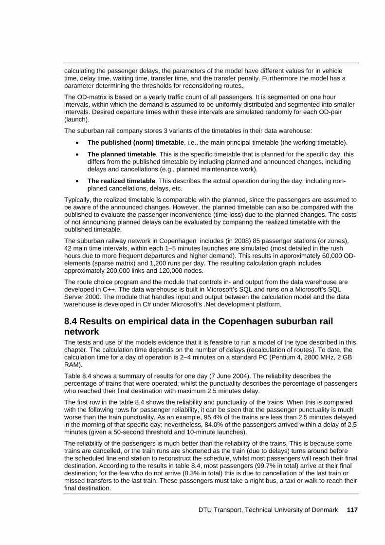
DTU Transport, Technical University of Denmark 117
calculating the passenger delays, the parameters of the model have different values for in vehicle time, delay time, waiting time, transfer time, and the transfer penalty. Furthermore the model has a parameter determining the thresholds for reconsidering routes.
The OD-matrix is based on a yearly traffic count of all passengers. It is segmented on one hour intervals, within which the demand is assumed to be uniformly distributed and segmented into smaller intervals. Desired departure times within these intervals are simulated randomly for each OD-pair (launch).
The suburban rail company stores 3 variants of the timetables in their data warehouse:
• The published (norm) timetable, i.e., the main principal timetable (the working timetable).
• The planned timetable. This is the specific timetable that is planned for the specific day, this differs from the published timetable by including planned and announced changes, including delays and cancellations (e.g., planned maintenance work).
• The realized timetable. This describes the actual operation during the day, including non-planed cancellations, delays, etc.
Typically, the realized timetable is comparable with the planned, since the passengers are assumed to be aware of the announced changes. However, the planned timetable can also be compared with the published to evaluate the passenger inconvenience (time loss) due to the planned changes. The costs of not announcing planned delays can be evaluated by comparing the realized timetable with the published timetable.
The suburban railway network in Copenhagen includes (in 2008) 85 passenger stations (or zones), 42 main time intervals, within each 1–5 minutes launches are simulated (most detailed in the rush hours due to more frequent departures and higher demand). This results in approximately 60,000 OD-elements (sparse matrix) and 1,200 runs per day. The resulting calculation graph includes approximately 200,000 links and 120,000 nodes.
The route choice program and the module that controls in- and output from the data warehouse are developed in C++. The data warehouse is built in Microsoft’s SQL and runs on a Microsoft’s SQL Server 2000. The module that handles input and output between the calculation model and the data warehouse is developed in C# under Microsoft’s .Net development platform.
8.4 Results on empirical data in the Copenhagen suburban rail network The tests and use of the models evidence that it is feasible to run a model of the type described in this chapter. The calculation time depends on the number of delays (recalculation of routes). To date, the calculation time for a day of operation is 2–4 minutes on a standard PC (Pentium 4, 2800 MHz, 2 GB RAM).
Table 8.4 shows a summary of results for one day (7 June 2004). The reliability describes the percentage of trains that were operated, whilst the punctuality describes the percentage of passengers who reached their final destination with maximum 2.5 minutes delay.
The first row in the table 8.4 shows the reliability and punctuality of the trains. When this is compared with the following rows for passenger reliability, it can be seen that the passenger punctuality is much worse than the train punctuality. As an example, 95.4% of the trains are less than 2.5 minutes delayed in the morning of that specific day; nevertheless, 84.0% of the passengers arrived within a delay of 2.5 minutes (given a 50-second threshold and 10-minute launches).
The reliability of the passengers is much better than the reliability of the trains. This is because some trains are cancelled, or the train runs are shortened as the train (due to delays) turns around before the scheduled line end station to reconstruct the schedule, whilst most passengers will reach their final destination. According to the results in table 8.4, most passengers (99.7% in total) arrive at their final destination; for the few who do not arrive (0.3% in total) this is due to cancellation of the last train or missed transfers to the last train. These passengers must take a night bus, a taxi or walk to reach their final destination.
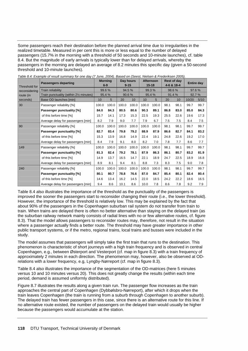
118 DTU Transport, Technical University of Denmark
Some passengers reach their destination before the planned arrival time due to irregularities in the realized timetable. Measured in per cent this is more or less equal to the number of delayed passengers (15.7% in the morning with a threshold of 50 seconds and 10-minute launches), cf. table 8.4. But the magnitude of early arrivals is typically lower than for delayed arrivals, whereby the passengers in the morning are delayed an average of 8.2 minutes this specific day (given a 50-second threshold and 10-minute launches). Table 8.4: Example of result summary for one day (7 June, 2004). Based on (Seest, Nielsen & Frederiksen 2005).
Threshold for reconsidering route (in seconds)
Passengers departing Morning 6-9
Day hours 9-15
Afternoon 15-18
Rest of day 4-6 & 18-4 Entire day
Train reliability 99.6 % 94.5 % 99.3 % 98.6 % 97.6 % Train punctuality (within 2½ minutes) 95.4 % 90.6 % 95.4 % 91.4 % 92.7 % Base OD launches [min] 10 5 20 10 10 5 20 10 10/20 5/10
30 Passenger reliability [%] 100.0 100.0 100.0 100.0 100.0 100.0 98.1 98.1 99.7 99.7 Passenger punctuality [%] 84.0 84.3 80.5 80.6 90.3 89.1 86.8 83.0 85.0 84.3 of this before time [%] 15.7 14.1 17.3 15.3 22.5 19.3 25.5 22.6 19.6 17.3 Average delay for passengers [min] 8.2 7.9 9.0 7.7 7.9 6.7 7.5 7.5 8.4 7.5
90 Passenger reliability [%] 100.0 100.0 100.0 100.0 100.0 100.0 98.1 98.1 99.7 99.7 Passenger punctuality [%] 82.7 83.4 79.8 79.2 88.9 87.9 86.6 82.7 84.1 83.2 of this before time [%] 15.3 13.9 16.8 14.9 22.4 19.1 24.8 22.6 19.2 17.0 Average delay for passengers [min] 8.4 7.9 9.1 8.0 8.2 7.0 7.8 7.7 8.6 7.7
149 Passenger reliability [%] 100.0 100.0 100.0 100.0 100.0 100.0 98.1 98.1 99.7 99.7 Passenger punctuality [%] 81.3 82.4 79.2 78.1 87.9 86.3 86.1 80.7 83.2 81.9 of this before time [%] 14.9 13.7 16.5 14.7 22.1 18.9 24.7 22.5 18.9 16.8 Average delay for passengers [min] 8.9 8.1 9.4 8.1 8.8 7.3 8.3 7.5 9.0 7.8
240 Passenger reliability [%] 100.0 100.0 100.0 100.0 100.0 100.0 98.1 98.1 99.7 99.7 Passenger punctuality [%] 80.1 80.7 78.8 76.6 87.0 84.7 85.4 80.1 82.4 80.4 of this before time [%] 14.6 13.4 16.2 14.5 22.0 18.5 24.2 22.2 18.6 16.5 Average delay for passengers [min] 9.4 8.6 10.1 8.6 10.0 7.8 8.6 7.8 9.2 7.9
Table 8.4 also illustrates the importance of the threshold as the punctuality of the passengers is improved the sooner the passengers start to reconsider changing their route (i.e., the lower threshold). However, the importance of the threshold is relatively low. This may be explained by the fact that about 90% of the passengers in the Copenhagen suburban rail system do not transfer from train to train. When trains are delayed there is often no better alternative than staying on the delayed train (as the suburban railway network mainly consists of radial lines with no or few alternative routes, cf. figure 8.3). That the model allows passengers to reconsider routes may, therefore, not result in the situation where a passenger actually finds a better route. The threshold may have greater importance in other public transport systems, or if the metro, regional trains, local trains and busses were included in the study.
The model assumes that passengers will simply take the first train that runs to the destination. This phenomenon is characteristic of short journeys with a high train frequency and is observed in central Copenhagen, e.g., between Østerport and Vesterport (cf. map in figure 8.3) with a train frequency of approximately 2 minutes in each direction. The phenomenon may, however, also be observed at OD-relations with a lower frequency, e.g, Lyngby-Nørreport (cf. map in figure 8.3).
Table 8.4 also illustrates the importance of the segmentation of the OD-matrices (here 5 minutes versus 10 and 10 minutes versus 20). This does not greatly change the results (within each time period, demand is assumed uniformly distributed).
Figure 8.7 illustrates the results along a given train run. The passenger flow increases as the train approaches the central part of Copenhagen (Dybbølsbro-Nørreport), after which it drops when the train leaves Copenhagen (the train is running from a suburb through Copenhagen to another suburb). The delayed train has fewer passengers in this case, since there is an alternative route for this line. If no alternative route existed, the number of passengers on the delayed train would usually be higher because the passengers would accumulate at the station.
DTU Transport, Technical University of Denmark 119
Train route B from Høje Taastrup to Holte, Train number 60126
0
50
100
150
200
250
300
350
Actual (delayed) timetable Planned timetable Seating capacity
Num
bero
f pas
seng
ers
Figure 8.7: Number of passengers in a specific train run, as a function of stations. The full-drawn line is the passenger flows on the delayed run and the broken line is the planned run. Based on (Seest, Nielsen & Frederiksen 2005).
8.5 Calculation of future passenger delays by simulation Calculating passenger delays of the performed operation is of interest to evaluate the system performance and to identify aspects or routines that could be improved. However, by combining the passenger delay model with a rail simulation model it is also possible to predict or estimate the future passenger delays. This can be used to evaluate changes in the infrastructure and/or in the timetables as early as in the planning phase.
Rail simulation software can be used to simulate the train delays of given planned timetables, in this case RailSys (Siefer, Radtke 2005). To do this, it is necessary to build up a detailed computer model of the infrastructure, interlocking system and the timetables to be simulated. The rules of operation are set up together with a set of delay distributions to simulate disturbances (cf. section 7.5 for further information).
Calculation of the passenger delays requires result data from the simulation of both the planned and all the realized/simulated timetables for all arrivals and departures. These data must be transferred from the railway simulation software to the passenger delay model. For this transformation a simple import-export tool has been developed in VB.Net.
The workflow of calculating the passenger delays is shown in figure 8.8. Here, the simulation of operation, export to the passenger delay model, and calculation of passenger delays simulates the impacts from one to several days of operation. To calibrate the model and to obtain a delay distribution, it is necessary to repeat this step a number of times before the evaluation is done (cf. chapter 7.5 for further information on calibration).
The rail simulation model is microscopic and describes rail infrastructure in detail (all tracks, switches, interlocking system, signals, blocks, etc.), whilst the passenger delay model runs only on a station to station basis. Therefore, there is a need to aggregate data when exporting this to the passenger delay model; it could be said that the data should be transformed from microscopic data to macroscopic data. (Nielsen, Frederiksen 2003) discuss these different levels of aggregation for rail transport networks (and public transport in general), and (Gille, Klemenz & Siefer 2008) discuss different aggregation levels for railway infrastructure data.
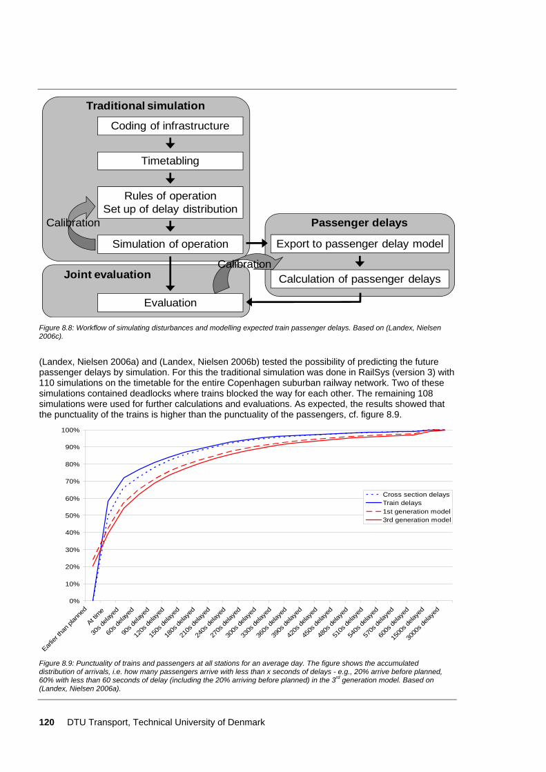
120 DTU Transport, Technical University of Denmark
Coding of infrastructure
Timetabling
Rules of operationSet up of delay distribution
Simulation of operation Export to passenger delay model
Calculation of passenger delays
Evaluation
Calibration
Joint evaluation
Passenger delays
Traditional simulation
Calibration
Figure 8.8: Workflow of simulating disturbances and modelling expected train passenger delays. Based on (Landex, Nielsen 2006c).
(Landex, Nielsen 2006a) and (Landex, Nielsen 2006b) tested the possibility of predicting the future passenger delays by simulation. For this the traditional simulation was done in RailSys (version 3) with 110 simulations on the timetable for the entire Copenhagen suburban railway network. Two of these simulations contained deadlocks where trains blocked the way for each other. The remaining 108 simulations were used for further calculations and evaluations. As expected, the results showed that the punctuality of the trains is higher than the punctuality of the passengers, cf. figure 8.9.
0%
10%
20%
30%
40%
50%
60%
70%
80%
90%
100%
Earlier
than
plan
ned
At time
30s d
elaye
d
60s d
elaye
d
90s d
elaye
d
120s
delay
ed
150s
delay
ed
180s
delay
ed
210s
delay
ed
240s
delay
ed
270s
delay
ed
300s
delay
ed
330s
delay
ed
360s
delay
ed
390s
delay
ed
420s
delay
ed
450s
delay
ed
480s
delay
ed
510s
delay
ed
540s
delay
ed
570s
delay
ed
600s
delay
ed
1500
s dela
yed
3000
s dela
yed
Cross section delaysTrain delays1st generation model3rd generation model
Figure 8.9: Punctuality of trains and passengers at all stations for an average day. The figure shows the accumulated distribution of arrivals, i.e. how many passengers arrive with less than x seconds of delays - e.g., 20% arrive before planned, 60% with less than 60 seconds of delay (including the 20% arriving before planned) in the 3rd generation model. Based on (Landex, Nielsen 2006a).
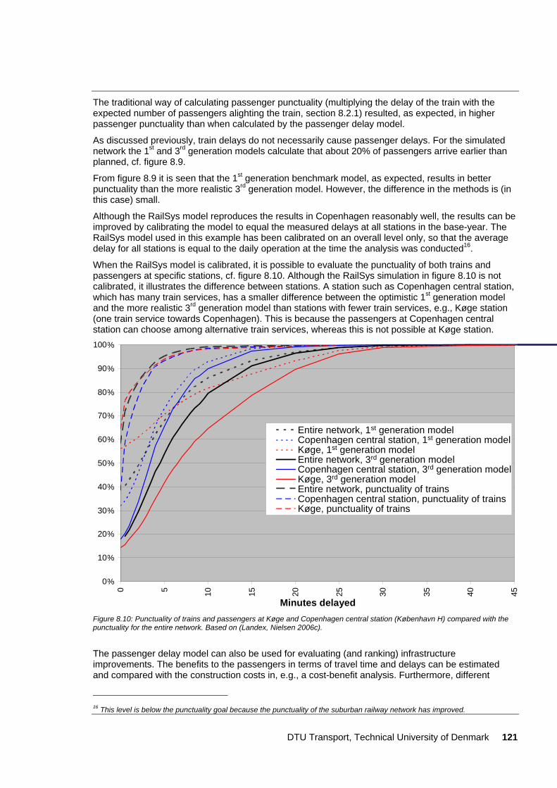
DTU Transport, Technical University of Denmark 121
The traditional way of calculating passenger punctuality (multiplying the delay of the train with the expected number of passengers alighting the train, section 8.2.1) resulted, as expected, in higher passenger punctuality than when calculated by the passenger delay model.
As discussed previously, train delays do not necessarily cause passenger delays. For the simulated network the 1st and 3rd generation models calculate that about 20% of passengers arrive earlier than planned, cf. figure 8.9.
From figure 8.9 it is seen that the 1st generation benchmark model, as expected, results in better punctuality than the more realistic 3rd generation model. However, the difference in the methods is (in this case) small.
Although the RailSys model reproduces the results in Copenhagen reasonably well, the results can be improved by calibrating the model to equal the measured delays at all stations in the base-year. The RailSys model used in this example has been calibrated on an overall level only, so that the average delay for all stations is equal to the daily operation at the time the analysis was conducted16.
When the RailSys model is calibrated, it is possible to evaluate the punctuality of both trains and passengers at specific stations, cf. figure 8.10. Although the RailSys simulation in figure 8.10 is not calibrated, it illustrates the difference between stations. A station such as Copenhagen central station, which has many train services, has a smaller difference between the optimistic 1st generation model and the more realistic 3rd generation model than stations with fewer train services, e.g., Køge station (one train service towards Copenhagen). This is because the passengers at Copenhagen central station can choose among alternative train services, whereas this is not possible at Køge station.
0,0%
10,0%
20,0%
30,0%
40,0%
50,0%
60,0%
70,0%
80,0%
90,0%
00,0%
0 5 10 15 20 25 30 35 40 45
Minutter forsinket
Total - Optimistisk passagerregularitetKøbenhavn H - Optimistisk passagerregularitetKøge - Optimistisk passagerregularitetTotal - PassagerregularitetKøbenhavn H - PassagerregularitetKøge - PassagerregularitetTotal - TogregularitetKøbenhavn H - TogregularitetKøge - Togregularitet
Minutes delayed
Entire network, 1st generation modelCopenhagen central station, 1st generation modelKøge, 1st generation modelEntire network, 3rd generation modelCopenhagen central station, 3rd generation modelKøge, 3rd generation modelEntire network, punctuality of trainsCopenhagen central station, punctuality of trainsKøge, punctuality of trains
0
10
20
30
40
50
60
70
80
90
100
Figure 8.10: Punctuality of trains and passengers at Køge and Copenhagen central station (København H) compared with the punctuality for the entire network. Based on (Landex, Nielsen 2006c).
The passenger delay model can also be used for evaluating (and ranking) infrastructure improvements. The benefits to the passengers in terms of travel time and delays can be estimated and compared with the construction costs in, e.g., a cost-benefit analysis. Furthermore, different
16 This level is below the punctuality goal because the punctuality of the suburban railway network has improved.
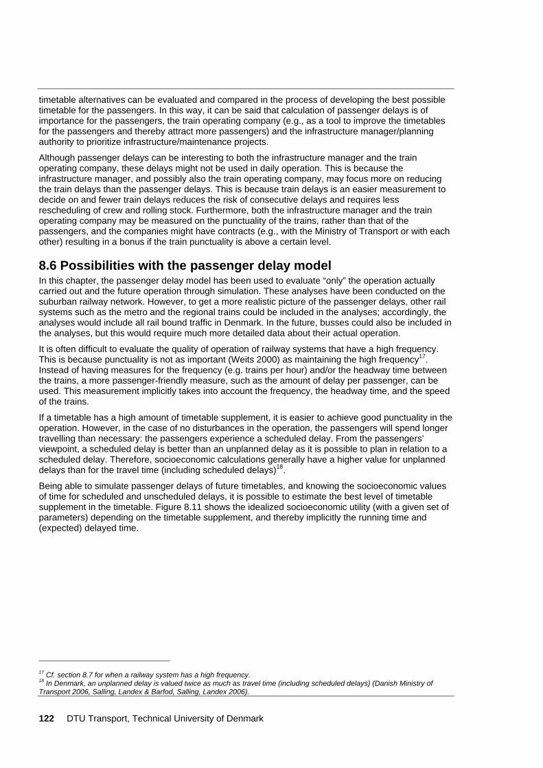
122 DTU Transport, Technical University of Denmark
timetable alternatives can be evaluated and compared in the process of developing the best possible timetable for the passengers. In this way, it can be said that calculation of passenger delays is of importance for the passengers, the train operating company (e.g., as a tool to improve the timetables for the passengers and thereby attract more passengers) and the infrastructure manager/planning authority to prioritize infrastructure/maintenance projects.
Although passenger delays can be interesting to both the infrastructure manager and the train operating company, these delays might not be used in daily operation. This is because the infrastructure manager, and possibly also the train operating company, may focus more on reducing the train delays than the passenger delays. This is because train delays is an easier measurement to decide on and fewer train delays reduces the risk of consecutive delays and requires less rescheduling of crew and rolling stock. Furthermore, both the infrastructure manager and the train operating company may be measured on the punctuality of the trains, rather than that of the passengers, and the companies might have contracts (e.g., with the Ministry of Transport or with each other) resulting in a bonus if the train punctuality is above a certain level.
8.6 Possibilities with the passenger delay model In this chapter, the passenger delay model has been used to evaluate “only” the operation actually carried out and the future operation through simulation. These analyses have been conducted on the suburban railway network. However, to get a more realistic picture of the passenger delays, other rail systems such as the metro and the regional trains could be included in the analyses; accordingly, the analyses would include all rail bound traffic in Denmark. In the future, busses could also be included in the analyses, but this would require much more detailed data about their actual operation.
It is often difficult to evaluate the quality of operation of railway systems that have a high frequency. This is because punctuality is not as important (Weits 2000) as maintaining the high frequency17. Instead of having measures for the frequency (e.g. trains per hour) and/or the headway time between the trains, a more passenger-friendly measure, such as the amount of delay per passenger, can be used. This measurement implicitly takes into account the frequency, the headway time, and the speed of the trains.
If a timetable has a high amount of timetable supplement, it is easier to achieve good punctuality in the operation. However, in the case of no disturbances in the operation, the passengers will spend longer travelling than necessary: the passengers experience a scheduled delay. From the passengers’ viewpoint, a scheduled delay is better than an unplanned delay as it is possible to plan in relation to a scheduled delay. Therefore, socioeconomic calculations generally have a higher value for unplanned delays than for the travel time (including scheduled delays)18.
Being able to simulate passenger delays of future timetables, and knowing the socioeconomic values of time for scheduled and unscheduled delays, it is possible to estimate the best level of timetable supplement in the timetable. Figure 8.11 shows the idealized socioeconomic utility (with a given set of parameters) depending on the timetable supplement, and thereby implicitly the running time and (expected) delayed time.
17 Cf. section 8.7 for when a railway system has a high frequency. 18 In Denmark, an unplanned delay is valued twice as much as travel time (including scheduled delays) (Danish Ministry of Transport 2006, Salling, Landex & Barfod, Salling, Landex 2006).
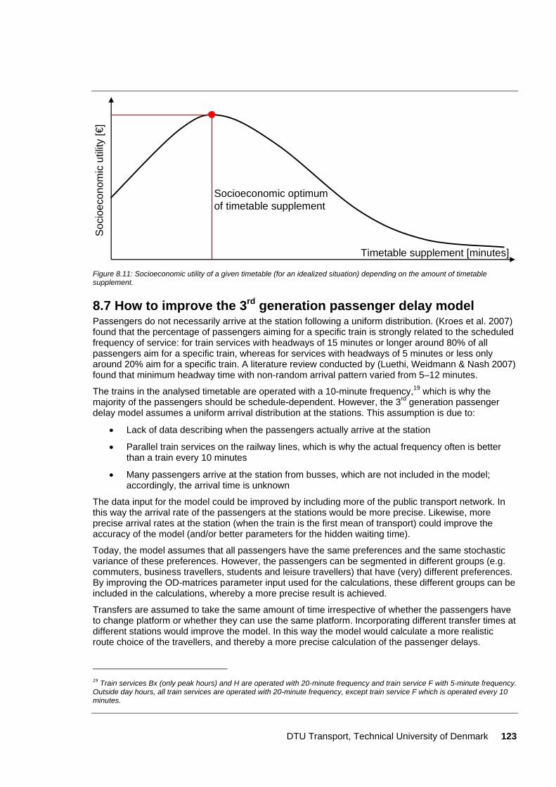
DTU Transport, Technical University of Denmark 123
Socioeconomic optimumof timetable supplement
Timetable supplement [minutes]
Soc
ioec
onom
ic u
tility
[€]
Figure 8.11: Socioeconomic utility of a given timetable (for an idealized situation) depending on the amount of timetable supplement.
8.7 How to improve the 3rd generation passenger delay model Passengers do not necessarily arrive at the station following a uniform distribution. (Kroes et al. 2007) found that the percentage of passengers aiming for a specific train is strongly related to the scheduled frequency of service: for train services with headways of 15 minutes or longer around 80% of all passengers aim for a specific train, whereas for services with headways of 5 minutes or less only around 20% aim for a specific train. A literature review conducted by (Luethi, Weidmann & Nash 2007) found that minimum headway time with non-random arrival pattern varied from 5–12 minutes.
The trains in the analysed timetable are operated with a 10-minute frequency,19 which is why the majority of the passengers should be schedule-dependent. However, the 3rd generation passenger delay model assumes a uniform arrival distribution at the stations. This assumption is due to:
• Lack of data describing when the passengers actually arrive at the station
• Parallel train services on the railway lines, which is why the actual frequency often is better than a train every 10 minutes
• Many passengers arrive at the station from busses, which are not included in the model; accordingly, the arrival time is unknown
The data input for the model could be improved by including more of the public transport network. In this way the arrival rate of the passengers at the stations would be more precise. Likewise, more precise arrival rates at the station (when the train is the first mean of transport) could improve the accuracy of the model (and/or better parameters for the hidden waiting time).
Today, the model assumes that all passengers have the same preferences and the same stochastic variance of these preferences. However, the passengers can be segmented in different groups (e.g. commuters, business travellers, students and leisure travellers) that have (very) different preferences. By improving the OD-matrices parameter input used for the calculations, these different groups can be included in the calculations, whereby a more precise result is achieved.
Transfers are assumed to take the same amount of time irrespective of whether the passengers have to change platform or whether they can use the same platform. Incorporating different transfer times at different stations would improve the model. In this way the model would calculate a more realistic route choice of the travellers, and thereby a more precise calculation of the passenger delays.
19 Train services Bx (only peak hours) and H are operated with 20-minute frequency and train service F with 5-minute frequency. Outside day hours, all train services are operated with 20-minute frequency, except train service F which is operated every 10 minutes.
124 DTU Transport, Technical University of Denmark
The model has a deterministic passenger choice function. This makes it possible to analyse the impact of delays exclusively without mixing this with other stochastic elements. A new version that includes overlapping routes (Probit-based error term) and random coefficients as in (Nielsen, Hansen & Daly 2001) could improve the results of the model.
8.8 Summary The chapter presents, classifies and discusses different methods and models to calculate passenger delays. The “0th generation” models that do not incorporate route choice models are highly inaccurate, whilst the 1st generation models that assume full knowledge on the delayed timetable systematically underestimate the passenger delays. The 2nd generation methods that simulate several timetables partly overcome this problem. The 3rd generation model formulated and presented in the chapter incorporates en route changes of decisions, whereby the passengers are first assumed to act on delays when they occur in time and space. This increases the accuracy of the model.
The chapter demonstrates that it is indeed possible to implement and run a 3rd generation passenger delay model for a network of the size of the Copenhagen suburban railway network. Dependent on the amount of delays, the run time of the model is 2–4 minutes. Since routes are recalculated when delays occur, the calculation time increases with the irregularity of the schedule.
The resulting passenger delays differed largely from the train delays in the Copenhagen suburban rail network. The difference between the train punctuality and passenger delays is due to the different number of passengers on the trains during the day, transfers between lines, and the fact that passengers (to some extent) will change routes due to delays. Furthermore, there is a higher risk of delays in rush hours due to more passengers and trains.
The chapter demonstrates how the 3rd generation passenger delay model can be combined with a rail simulation model. This makes it possible to calculate the expected passenger delays in a future planned timetable by simulation. The evaluation of passenger delays is obtained with a railway operation simulation software, RailSys, and the passenger delay model was comparable with the daily operation of the Copenhagen suburban network. Using a well-calibrated RailSys model will make it possible to compare travel times and delays for different future scenarios; for changes in the infrastructure as well as in timetables.
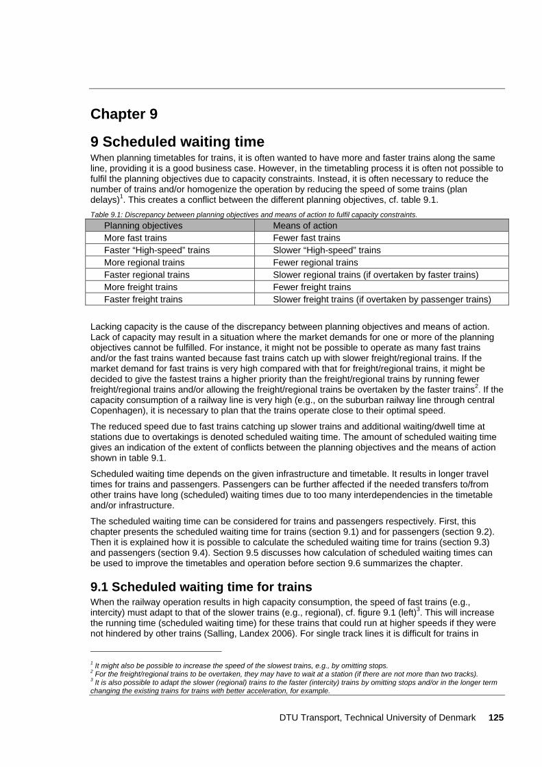
DTU Transport, Technical University of Denmark 125
Chapter 9
9 Scheduled waiting time When planning timetables for trains, it is often wanted to have more and faster trains along the same line, providing it is a good business case. However, in the timetabling process it is often not possible to fulfil the planning objectives due to capacity constraints. Instead, it is often necessary to reduce the number of trains and/or homogenize the operation by reducing the speed of some trains (plan delays)1. This creates a conflict between the different planning objectives, cf. table 9.1. Table 9.1: Discrepancy between planning objectives and means of action to fulfil capacity constraints.
Planning objectives Means of action More fast trains Fewer fast trains Faster “High-speed” trains Slower “High-speed” trains More regional trains Fewer regional trains Faster regional trains Slower regional trains (if overtaken by faster trains) More freight trains Fewer freight trains Faster freight trains Slower freight trains (if overtaken by passenger trains)
Lacking capacity is the cause of the discrepancy between planning objectives and means of action. Lack of capacity may result in a situation where the market demands for one or more of the planning objectives cannot be fulfilled. For instance, it might not be possible to operate as many fast trains and/or the fast trains wanted because fast trains catch up with slower freight/regional trains. If the market demand for fast trains is very high compared with that for freight/regional trains, it might be decided to give the fastest trains a higher priority than the freight/regional trains by running fewer freight/regional trains and/or allowing the freight/regional trains be overtaken by the faster trains2. If the capacity consumption of a railway line is very high (e.g., on the suburban railway line through central Copenhagen), it is necessary to plan that the trains operate close to their optimal speed.
The reduced speed due to fast trains catching up slower trains and additional waiting/dwell time at stations due to overtakings is denoted scheduled waiting time. The amount of scheduled waiting time gives an indication of the extent of conflicts between the planning objectives and the means of action shown in table 9.1.
Scheduled waiting time depends on the given infrastructure and timetable. It results in longer travel times for trains and passengers. Passengers can be further affected if the needed transfers to/from other trains have long (scheduled) waiting times due to too many interdependencies in the timetable and/or infrastructure.
The scheduled waiting time can be considered for trains and passengers respectively. First, this chapter presents the scheduled waiting time for trains (section 9.1) and for passengers (section 9.2). Then it is explained how it is possible to calculate the scheduled waiting time for trains (section 9.3) and passengers (section 9.4). Section 9.5 discusses how calculation of scheduled waiting times can be used to improve the timetables and operation before section 9.6 summarizes the chapter.
9.1 Scheduled waiting time for trains When the railway operation results in high capacity consumption, the speed of fast trains (e.g., intercity) must adapt to that of the slower trains (e.g., regional), cf. figure 9.1 (left)3. This will increase the running time (scheduled waiting time) for these trains that could run at higher speeds if they were not hindered by other trains (Salling, Landex 2006). For single track lines it is difficult for trains in
1 It might also be possible to increase the speed of the slowest trains, e.g., by omitting stops. 2 For the freight/regional trains to be overtaken, they may have to wait at a station (if there are not more than two tracks). 3 It is also possible to adapt the slower (regional) trains to the faster (intercity) trains by omitting stops and/or in the longer term changing the existing trains for trains with better acceleration, for example.

126 DTU Transport, Technical University of Denmark
different directions to pass each other, which can result in additional dwelling time at the crossing stations (scheduled waiting time), cf. figure 9.1 (right).
Sche
dule
dw
aitin
gtim
e
Station 1 Station 2 Station 3 Station 4 Station 5
Sche
dule
dw
aitin
gtim
e
Time
Distnance
Time
Sche
dule
dw
aitin
gtim
e
Figure 9.1: Extended running time (scheduled waiting time) for trains due to other trains on the railway line (double track on the right and single track on the left). Partly based on (Salling, Landex 2006).
Scheduled waiting time for trains can be added to the dwell time at stations and to the running time (Pachl 2008). In Norway, travel time is extended by scheduled waiting time at the railway lines in the suburbs (Skartsæterhagen 1993). In the Netherlands, the stations at The Hauge (The Hauge Holland Spoor and The Hauge Central Station) are examples of stations where the dwell time has been extended due to conflicts with other trains (Nie, Hansen 2005). It can therefore be argued whether there is scheduled waiting time at the stations at The Hauge.
If the scheduled waiting time is high, it might be decided to use this time, or part of it, to include extra stops for the fastest train services, cf. figure 9.2. In this way the planned timetable has trains with more stops than desired in the wanted timetable. It is difficult to evaluate scheduled waiting time when it, or some of it, has already been converted into additional stops as it is difficult/impossible to identify the stops that have been added to the timetable.
Sch
edul
edw
aitin
g tim
e
Time
Place
Wanted train path
Planned train path
Conflicting train path
Figure 9.2: Scheduled waiting time due to extra stops (Landex, Nielsen 2007a).
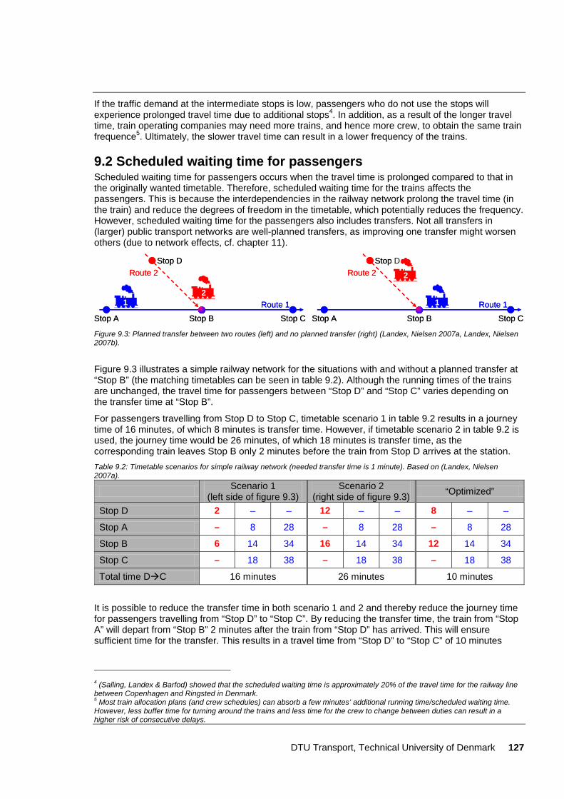
DTU Transport, Technical University of Denmark 127
If the traffic demand at the intermediate stops is low, passengers who do not use the stops will experience prolonged travel time due to additional stops4. In addition, as a result of the longer travel time, train operating companies may need more trains, and hence more crew, to obtain the same train frequence5. Ultimately, the slower travel time can result in a lower frequency of the trains.
9.2 Scheduled waiting time for passengers Scheduled waiting time for passengers occurs when the travel time is prolonged compared to that in the originally wanted timetable. Therefore, scheduled waiting time for the trains affects the passengers. This is because the interdependencies in the railway network prolong the travel time (in the train) and reduce the degrees of freedom in the timetable, which potentially reduces the frequency. However, scheduled waiting time for the passengers also includes transfers. Not all transfers in (larger) public transport networks are well-planned transfers, as improving one transfer might worsen others (due to network effects, cf. chapter 11).
21 Route 1
Route 2
Stop CStop BStop A
Stop D
21 Route 1
Route 2
Stop CStop BStop A
Stop D
2
1 Route 1
Route 2
Stop CStop BStop A
Stop D
22
11 Route 1
Route 2
Stop CStop BStop A
Stop D
Figure 9.3: Planned transfer between two routes (left) and no planned transfer (right) (Landex, Nielsen 2007a, Landex, Nielsen 2007b).
Figure 9.3 illustrates a simple railway network for the situations with and without a planned transfer at “Stop B” (the matching timetables can be seen in table 9.2). Although the running times of the trains are unchanged, the travel time for passengers between “Stop D” and “Stop C” varies depending on the transfer time at “Stop B”.
For passengers travelling from Stop D to Stop C, timetable scenario 1 in table 9.2 results in a journey time of 16 minutes, of which 8 minutes is transfer time. However, if timetable scenario 2 in table 9.2 is used, the journey time would be 26 minutes, of which 18 minutes is transfer time, as the corresponding train leaves Stop B only 2 minutes before the train from Stop D arrives at the station. Table 9.2: Timetable scenarios for simple railway network (needed transfer time is 1 minute). Based on (Landex, Nielsen 2007a).
Scenario 1 (left side of figure 9.3)
Scenario 2 (right side of figure 9.3) “Optimized”
Stop D 2 – – 12 – – 8 – –
Stop A – 8 28 – 8 28 – 8 28
Stop B 6 14 34 16 14 34 12 14 34
Stop C – 18 38 – 18 38 – 18 38
Total time D C 16 minutes 26 minutes 10 minutes It is possible to reduce the transfer time in both scenario 1 and 2 and thereby reduce the journey time for passengers travelling from “Stop D” to “Stop C”. By reducing the transfer time, the train from “Stop A” will depart from “Stop B” 2 minutes after the train from “Stop D” has arrived. This will ensure sufficient time for the transfer. This results in a travel time from “Stop D” to “Stop C” of 10 minutes
4 (Salling, Landex & Barfod) showed that the scheduled waiting time is approximately 20% of the travel time for the railway line between Copenhagen and Ringsted in Denmark. 5 Most train allocation plans (and crew schedules) can absorb a few minutes’ additional running time/scheduled waiting time. However, less buffer time for turning around the trains and less time for the crew to change between duties can result in a higher risk of consecutive delays.
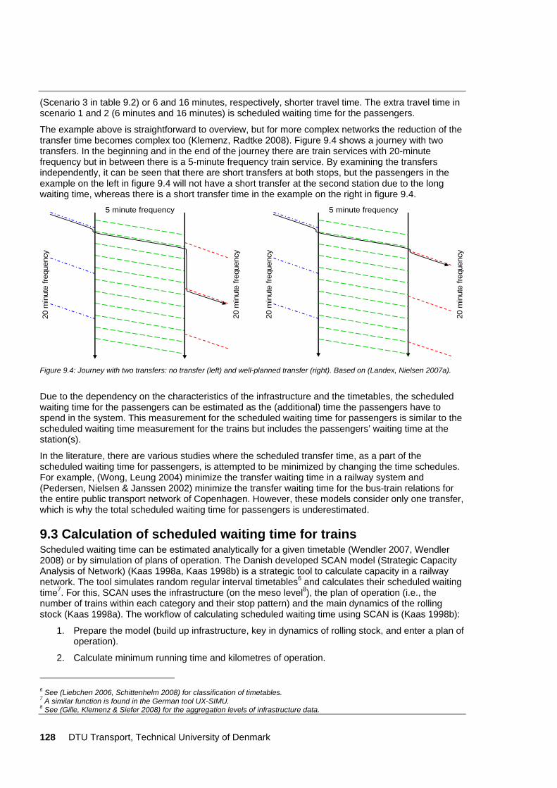
128 DTU Transport, Technical University of Denmark
(Scenario 3 in table 9.2) or 6 and 16 minutes, respectively, shorter travel time. The extra travel time in scenario 1 and 2 (6 minutes and 16 minutes) is scheduled waiting time for the passengers.
The example above is straightforward to overview, but for more complex networks the reduction of the transfer time becomes complex too (Klemenz, Radtke 2008). Figure 9.4 shows a journey with two transfers. In the beginning and in the end of the journey there are train services with 20-minute frequency but in between there is a 5-minute frequency train service. By examining the transfers independently, it can be seen that there are short transfers at both stops, but the passengers in the example on the left in figure 9.4 will not have a short transfer at the second station due to the long waiting time, whereas there is a short transfer time in the example on the right in figure 9.4.
5 minute frequency
20 m
inut
e fre
quen
cy
20 m
inut
e fre
quen
cy
5 minute frequency
20 m
inut
e fre
quen
cy
20 m
inut
e fre
quen
cy
Figure 9.4: Journey with two transfers: no transfer (left) and well-planned transfer (right). Based on (Landex, Nielsen 2007a).
Due to the dependency on the characteristics of the infrastructure and the timetables, the scheduled waiting time for the passengers can be estimated as the (additional) time the passengers have to spend in the system. This measurement for the scheduled waiting time for passengers is similar to the scheduled waiting time measurement for the trains but includes the passengers’ waiting time at the station(s).
In the literature, there are various studies where the scheduled transfer time, as a part of the scheduled waiting time for passengers, is attempted to be minimized by changing the time schedules. For example, (Wong, Leung 2004) minimize the transfer waiting time in a railway system and (Pedersen, Nielsen & Janssen 2002) minimize the transfer waiting time for the bus-train relations for the entire public transport network of Copenhagen. However, these models consider only one transfer, which is why the total scheduled waiting time for passengers is underestimated.
9.3 Calculation of scheduled waiting time for trains Scheduled waiting time can be estimated analytically for a given timetable (Wendler 2007, Wendler 2008) or by simulation of plans of operation. The Danish developed SCAN model (Strategic Capacity Analysis of Network) (Kaas 1998a, Kaas 1998b) is a strategic tool to calculate capacity in a railway network. The tool simulates random regular interval timetables6 and calculates their scheduled waiting time7. For this, SCAN uses the infrastructure (on the meso level8), the plan of operation (i.e., the number of trains within each category and their stop pattern) and the main dynamics of the rolling stock (Kaas 1998a). The workflow of calculating scheduled waiting time using SCAN is (Kaas 1998b):
1. Prepare the model (build up infrastructure, key in dynamics of rolling stock, and enter a plan of operation).
2. Calculate minimum running time and kilometres of operation.
6 See (Liebchen 2006, Schittenhelm 2008) for classification of timetables. 7 A similar function is found in the German tool UX-SIMU. 8 See (Gille, Klemenz & Siefer 2008) for the aggregation levels of infrastructure data.
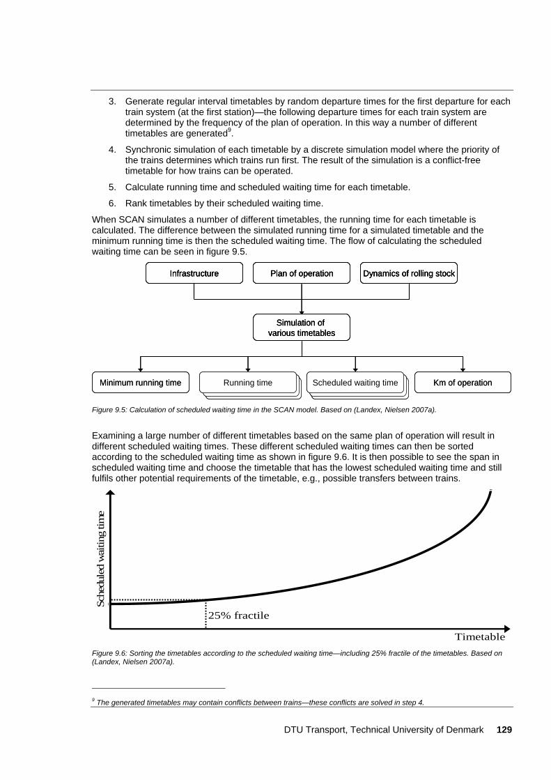
DTU Transport, Technical University of Denmark 129
3. Generate regular interval timetables by random departure times for the first departure for each train system (at the first station)—the following departure times for each train system are determined by the frequency of the plan of operation. In this way a number of different timetables are generated9.
4. Synchronic simulation of each timetable by a discrete simulation model where the priority of the trains determines which trains run first. The result of the simulation is a conflict-free timetable for how trains can be operated.
5. Calculate running time and scheduled waiting time for each timetable.
6. Rank timetables by their scheduled waiting time.
When SCAN simulates a number of different timetables, the running time for each timetable is calculated. The difference between the simulated running time for a simulated timetable and the minimum running time is then the scheduled waiting time. The flow of calculating the scheduled waiting time can be seen in figure 9.5.
Running time Scheduled waiting time Km of operationMinimum running time
Simulation of various timetables
Infrastructure Plan of operation Dynamics of rolling stock
Running time Scheduled waiting time Km of operationMinimum running time
Simulation of various timetables
Simulation of various timetables
Infrastructure Plan of operation Dynamics of rolling stockInfrastructure Plan of operation Dynamics of rolling stock
Figure 9.5: Calculation of scheduled waiting time in the SCAN model. Based on (Landex, Nielsen 2007a).
Examining a large number of different timetables based on the same plan of operation will result in different scheduled waiting times. These different scheduled waiting times can then be sorted according to the scheduled waiting time as shown in figure 9.6. It is then possible to see the span in scheduled waiting time and choose the timetable that has the lowest scheduled waiting time and still fulfils other potential requirements of the timetable, e.g., possible transfers between trains.
Timetable
Sche
dule
d w
aitin
g tim
e
25% fractile
Figure 9.6: Sorting the timetables according to the scheduled waiting time—including 25% fractile of the timetables. Based on (Landex, Nielsen 2007a).
9 The generated timetables may contain conflicts between trains—these conflicts are solved in step 4.
130 DTU Transport, Technical University of Denmark
When evaluating the scheduled waiting time of a plan of operation (on a given infrastructure) the final (chosen) timetable is not necessarily the timetable with the lowest scheduled waiting time as this timetable is, in general, without interest in practice (Kaas 1998b). For instance, this can be due to lack of transfers for the passengers and too much bundling of the trains resulting in reduced service for the passengers. Therefore, the 25% fractile has been chosen in Denmark to describe a satisfactory quality of operation, and thereby the expected scheduled waiting time of the plan of operation (Kaas 1998b).
A problem with the SCAN model is that timetable supplements to catch up smaller delays are not included, which is why the model can be used only to evaluate the plan of operation. Alternatively, the North American Train Performance Calculator (TPC) (White 2007) can be used to generate a large number of timetables, which can be investigated. The workflow in the TPC model is (based on (White 2007)):
1. Prepare the model (build up infrastructure, key in dynamics of rolling stock and train services)
2. Generate timetables randomly by choosing random departure times for all trains
3. Simulation of each timetable to generate conflict-free timetables
Based on the results of the TPC-model, it is possible to calculate the running times of the timetables. However, to examine the scheduled waiting times it is necessary to calculate the minimum running time of the train services too. When the scheduled waiting times of the timetables have been calculated it is possible to rank the timetables by scheduled waiting times as in figure 9.6. The major differences between the TPC and SCAN models are that the SCAN model examines randomly generated regular interval timetables, while TPC examines timetables where all the trains are operated randomly; furthermore, SCAN calculates the scheduled waiting time itself, whereas the calculation has to be done manually in the TPC model.
In North America, the trains are operated according to a more or less improvised timetable (Pachl 2008, White 2005), which is why the TPC model is well suited there. This random operation is possible because most of the trains operated are freight trains10. However, in Denmark (and Europe) the operation is mostly based on regular interval timetables; accordingly, the TPC model is less suited to simulate the operation there. The SCAN model simulates regular interval timetables but does not include timetable supplements. To have a better simulation model well suited for analyses in the Danish/European context, the SCAN model should be developed to include timetable supplements, and/or the TPC model should be adapted to examine regular interval timetables.
Generally, simulation models based on future plans of operation are well suited for strategic analyses, but it is difficult to examine where the capacity problems, and thereby the scheduled waiting time, are the most severe. Consequently, it is also difficult to examine where the infrastructure should be improved and what effects the improvement will have. Combining microscopic and macroscopic models can, however, help in this kind of analysis. Railnet Austria has the combination of microscopic and macroscopic models in the infrastructure planning (Sewcyk, Radtke & Wilfinger 2007). Here, future timetables have been developed and evaluated (in this case by UIC 406) by converting data between the macroscopic and microscopic level (Sewcyk, Radtke & Wilfinger 2007); the methodology could be the basis when evaluating scheduled waiting time for different timetable alternatives.
9.4 Calculation of scheduled waiting time for passengers Scheduled waiting time for passengers is the delay of the passengers compared with that of the “optimal” timetable. This definition is very similar to the scheduled waiting time for trains. However, cases with a small amount of scheduled waiting time for trains do not necessarily result in a small amount of scheduled waiting time for passengers—and vice versa. This is because only a few minutes of scheduled waiting time for a train might result in a lost transfer for the passengers, but only if the transfer time is tight, otherwise the total travel time remains unchanged.
The SCAN model used to calculate scheduled waiting times for trains (Kaas 1998b) can be used to calculate scheduled waiting times for passengers too. This is because the output timetables from
10 Certain corridors have many passenger trains.
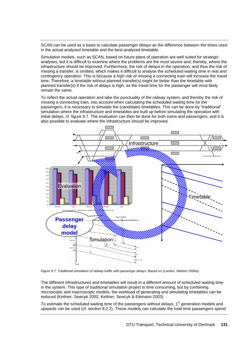
DTU Transport, Technical University of Denmark 131
SCAN can be used as a basis to calculate passenger delays as the difference between the times used in the actual analysed timetable and the best-analyzed timetable.
Simulation models, such as SCAN, based on future plans of operation are well suited for strategic analyses, but it is difficult to examine where the problems are the most severe and, thereby, where the infrastructure should be improved. Furthermore, the risk of delays in the operation, and thus the risk of missing a transfer, is omitted, which makes it difficult to analyse the scheduled waiting time in real and contingency operation. This is because a high risk of missing a connecting train will increase the travel time. Therefore, a timetable without planned transfer(s) might be better than the timetable with planned transfer(s) if the risk of delays is high, as the travel time for the passenger will most likely remain the same.
To reflect the actual operation and take the punctuality of the railway system, and thereby the risk of missing a connecting train, into account when calculating the scheduled waiting time for the passengers, it is necessary to simulate the (candidate) timetables. This can be done by “traditional” simulation where the infrastructure and timetables are built up before simulating the operation with initial delays, cf. figure 9.7. The evaluation can then be done for both trains and passengers, and it is also possible to evaluate where the infrastructure should be improved.
95,4%
84,0%
15,7%
90,6%
80,5%
17,3%
95,4%90,3%
22,5%
91,4%86,8%
22,5%
92,7%
85,0%
19,6%
0%
10%
20%
30%
40%
50%
60%
70%
80%
90%
100%
Morning Day Afternoon Other time Total
Train regularity [%] Passenger regularity [%] Arrivals before time [%]
Infrastructure
Timetable
Evaluation
Simulation
Passengerdelaymodel
Figure 9.7: Traditional simulation of railway traffic with passenger delays. Based on (Landex, Nielsen 2006a).
The different infrastructures and timetables will result in a different amount of scheduled waiting time in the system. This type of traditional simulation project is time consuming, but by combining microscopic and macroscopic models, the workload of generating and simulating timetables can be reduced (Kettner, Sewcyk 2002, Kettner, Sewcyk & Eikmann 2003).
To estimate the scheduled waiting time of the passengers without delays, 1st generation models and upwards can be used (cf. section 8.2.2). These models can calculate the total time passengers spend
132 DTU Transport, Technical University of Denmark
in the railway system, whereby passengers’ scheduled waiting time can be deduced. However, 3rd generation models (cf. section 8.2.5) are the best if the scheduled waiting time is to be calculated in the case of train delays or if sensitivity analyses have to be done. As 3rd generation models require the same work effort as 1st, 1½ and 2nd generation models, the thesis recommends that 3rd generation models are used.
9.5 Discussion Timetables in railway networks can be improved by examining scheduled waiting times in the planning process. By examining scheduled waiting times for different future (candidate) timetables, it is possible to examine different timetable strategies, for example, additional overtaking. When examining an additional overtaking, it is possible to evaluate both the time gain for the passengers in the fast train and the time loss for the passengers in the train that is overtaken. This examination can be done either locally for a single railway line or for the entire system including transfers to/from other trains.
Improving the timetables without taking the risk of delays into account can result in an over-optimized timetable for passengers. This is because even small delays will result in lost transfers for the passenger or even degenerated schedules. To take common delays into account, the thesis recommends simulation of the timetables with a typical delay distribution. The additional scheduled waiting time for the passengers can then be calculated based on the simulated timetables. This makes it possible to optimize the timetables for both trains and passengers and, thereby, make the timetables robust to delays.
Optimizing the scheduled waiting time is not possible in all types of timetable, for example, in an integrated fixed interval timetable11 where all trains meet at the same time at stations/hubs throughout the network. In integrated fixed interval timetables the structure of the timetable is fixed when the stations/hubs have been selected. Additionally, the scheduled waiting time has virtually been determined by the chosen stations/hubs as all the trains have to meet at the station/hub and a train is not permitted to leave before the last train has arrived (and the passengers have had time to make the transfer). Therefore, scheduled waiting time cannot be optimized in integrated fixed interval timetables, but the amount of scheduled waiting time can be used to describe how well the infrastructure can handle the chosen integrated fixed interval timetable.
In the longer term this approach can also be used by the centralized control offices to decide if a train should wait for a delayed train to obtain the transfer. Thus, the simulation of the traffic combined with calculating the scheduled waiting times for trains and passengers can be used to evaluate the consequences of different scenarios. In this way it is possible to improve the operation.
The short-term operation can be improved too by including evaluation of scheduled waiting times in the planning process. Timetables can be simulated and scheduled waiting times for both trains and passengers can be calculated so that the best possible timetable is chosen. This approach can also be used when planning timetables for contingency operation, so the best timetable can be used in cases of disrupted operation.
9.6 Summary Railway operation is often affected by scheduled waiting time because fast trains (due to infrastructure restrictions) cannot overtake slower trains. This means that additional time—scheduled delays—has to be implemented in the timetable. The additional time affects both the trains and the passengers in them. However, the passengers are also affected by scheduled waiting time in the case of transfers.
Scheduled waiting time for trains can be calculated by simulation models such as the Danish SCAN model and the North American TPC model. Based on the scheduled waiting time for trains and passenger delay models (1st generation and upwards) it is possible to calculate the scheduled waiting time for passengers. It is also possible to estimate the scheduled waiting time in the case of delays. In this case the thesis recommends that the 3rd generation passenger delay model is used because it is
11 See (Liebchen 2006, Schittenhelm 2008) for classification of timetables.

DTU Transport, Technical University of Denmark 133
the most precise passenger delay model and does not require more work effort than previous generations of passenger delay models.
Calculating scheduled waiting times for candidate timetables makes it possible to test different timetable strategies and choose the best strategy for the final timetable. This can improve the timetables for both the operator(s) and the passengers. In the longer term, the approach can be used at the centralized control offices for contingency operation. Here, an evaluation of the scheduled waiting time can be used to choose the dispatching strategy that results in the fewest delays for trains and passengers.

134 DTU Transport, Technical University of Denmark
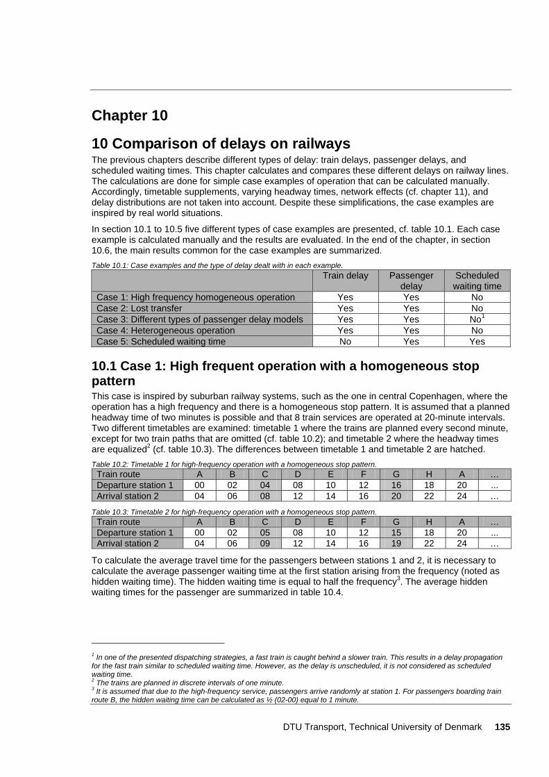
DTU Transport, Technical University of Denmark 135
Chapter 10
10 Comparison of delays on railways The previous chapters describe different types of delay: train delays, passenger delays, and scheduled waiting times. This chapter calculates and compares these different delays on railway lines. The calculations are done for simple case examples of operation that can be calculated manually. Accordingly, timetable supplements, varying headway times, network effects (cf. chapter 11), and delay distributions are not taken into account. Despite these simplifications, the case examples are inspired by real world situations.
In section 10.1 to 10.5 five different types of case examples are presented, cf. table 10.1. Each case example is calculated manually and the results are evaluated. In the end of the chapter, in section 10.6, the main results common for the case examples are summarized. Table 10.1: Case examples and the type of delay dealt with in each example. Train delay Passenger
delay Scheduled waiting time
Case 1: High frequency homogeneous operation Yes Yes No Case 2: Lost transfer Yes Yes No Case 3: Different types of passenger delay models Yes Yes No1 Case 4: Heterogeneous operation Yes Yes No Case 5: Scheduled waiting time No Yes Yes
10.1 Case 1: High frequent operation with a homogeneous stop pattern This case is inspired by suburban railway systems, such as the one in central Copenhagen, where the operation has a high frequency and there is a homogeneous stop pattern. It is assumed that a planned headway time of two minutes is possible and that 8 train services are operated at 20-minute intervals. Two different timetables are examined: timetable 1 where the trains are planned every second minute, except for two train paths that are omitted (cf. table 10.2); and timetable 2 where the headway times are equalized2 (cf. table 10.3). The differences between timetable 1 and timetable 2 are hatched. Table 10.2: Timetable 1 for high-frequency operation with a homogeneous stop pattern.
Train route A B C D E F G H A … Departure station 1 00 02 04 08 10 12 16 18 20 ... Arrival station 2 04 06 08 12 14 16 20 22 24 …
Table 10.3: Timetable 2 for high-frequency operation with a homogeneous stop pattern. Train route A B C D E F G H A … Departure station 1 00 02 05 08 10 12 15 18 20 ... Arrival station 2 04 06 09 12 14 16 19 22 24 …
To calculate the average travel time for the passengers between stations 1 and 2, it is necessary to calculate the average passenger waiting time at the first station arising from the frequency (noted as hidden waiting time). The hidden waiting time is equal to half the frequency3. The average hidden waiting times for the passenger are summarized in table 10.4.
1 In one of the presented dispatching strategies, a fast train is caught behind a slower train. This results in a delay propagation for the fast train similar to scheduled waiting time. However, as the delay is unscheduled, it is not considered as scheduled waiting time. 2 The trains are planned in discrete intervals of one minute. 3 It is assumed that due to the high-frequency service, passengers arrive randomly at station 1. For passengers boarding train route B, the hidden waiting time can be calculated as ½·(02-00) equal to 1 minute.
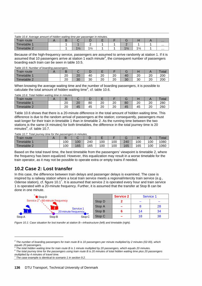
136 DTU Transport, Technical University of Denmark
Table 10.4: Average amount of hidden waiting time per passenger in minutes. Train route A B C D E F G H A … Timetable 1 1 1 2 1 1 2 1 1 ... Timetable 2 1 1½ 1½ 1 1 1½ 1½ 1 …
Because of the high-frequency service, passengers are assumed to arrive randomly at station 1. If it is assumed that 10 passengers arrive at station 1 each minute4, the consequent number of passengers boarding each train can be seen in table 10.5. Table 10.5: Number of boarding passengers.
Train route A B C D E F G H A Total Timetable 1 20 20 40 20 20 40 20 20 200 Timetable 2 20 30 30 20 20 30 30 20 200
When knowing the average waiting time and the number of boarding passengers, it is possible to calculate the total amount of hidden waiting time5, cf. table 10.6. Table 10.6: Total hidden waiting time in minutes.
Train route A B C D E F G H A Total Timetable 1 20 20 80 20 20 80 20 20 280 Timetable 2 20 45 45 20 20 45 45 20 260
Table 10.6 shows that there is a 20-minute difference in the total amount of hidden waiting time. This difference is due to the random arrival of passengers at the station; consequently, passengers must wait longer for their train in timetable 1 than in timetable 2. As the running time between the two stations is the same (4 minutes) for both timetables, the difference in the total journey time is 20 minutes6, cf. table 10.7. Table 10.7: Total journey time for the passengers in minutes.
Train route A B C D E F G H A Total Timetable 1 100 100 240 100 100 240 100 100 1080 Timetable 2 100 165 165 100 100 165 165 100 1060
Based on the total travel time, the best timetable from the passengers’ viewpoint is timetable 2, where the frequency has been equalized. However, this equalization may result in a worse timetable for the train operator, as it may not be possible to operate extra or empty trains if needed.
10.2 Case 2: Lost transfer In this case, the difference between train delays and passenger delays is examined. The case is inspired by a railway station where a local train service meets a regional/intercity train service (e.g., Odense station), cf. figure 10.17. It is assumed that service 2 is operated every hour and train service 1 is operated with a 20-minute frequency. Further, it is assumed that the transfer at Stop B can be done in one minute.
21
Service 1
Service 2
Stop CStop BStop A
Stop D60 minute frequency
20 minute frequency
Service 2 Service 1 Stop D 2 – – Stop A – 8 28 Stop B 6 14 34 Stop C – 18 38
Figure 10.1: Case situation for lost transfer at station B—infrastructure (left) and timetable (right).
4 The number of boarding passengers for train route B is 10 passengers per minute multiplied by 2 minutes (02-00), which equals 20 passengers. 5 The total hidden waiting time for train route B is 1 minute multiplied by 20 passengers, which equals 20 minutes. 6 The total journey time for the passengers using train route B is 20 minutes of total hidden waiting time plus 20 passengers multiplied by 4 minutes of travel time. 7 The case example is identical to scenario 1 in section 9.2.

DTU Transport, Technical University of Denmark 137
Because train service 2 is operated only hourly, it is assumed that all passengers will be at the station at the planned time of departure from Stop D. Accordingly, passenger delays can be calculated based on the delay of the trains only, cf. figure 10.2.
0
5
10
15
20
25
30
35
40
45
0 5 10 15 20 25 30Train delay in minutes
Ave
rage
pas
seng
er d
elay
in m
inut
es..
Figure 10.2: Train delay of train service 2 versus average passenger delay for passengers travelling from Stop D to Stop C.
Figure 10.2 shows that the train delay differs on train service 2 from the average passenger delay for passengers travelling from Stop D to Stop C. Sometimes, the average passenger delay is smaller than the train delay; in other cases the situation is reversed. The difference is caused by the transfer: if the transfer is missed, the passenger delay increases by the waiting time for the next service8. However, train service 2 might experience a “small” delay (i.e., less than 7 minutes) without the passengers arriving late at Stop C, because the transfer is not missed.
When the number of passengers on the trains is known, it is possible to calculate whether it is beneficial to allow the corresponding train to wait for the first train to arrive. The thesis suggests this is done by choosing the strategy that has the lowest amount of passenger delay. It is also possible to establish rules regarding the amount of time a train is allowed to wait for a delayed train by examining when the overall amount of passenger delay starts to increase9.
When knowing both the OD-matrix of the passengers and the delay distributions, it is possible to simulate candidate timetables and calculate passenger delays. In this way it is possible to choose the timetable with the best transfer times10. This kind of calculation is relevant when planning, e.g., the cross line of the Copenhagen suburban railway network, which is operated independently from the other railway lines and has transfer possibilities with all the other lines.
10.3 Case 3: Optimistic versus 3rd generation passenger delay models 1st and 1½ generation passenger delay models use an optimistic method to calculate the delays as it is assumed that the passengers have full knowledge of the delays. In contrast, 3rd generation
8 In the case of a mixed service with fast trains and trains stopping at all stations, the passenger delay will also depend on which service the passenger had planned to use and which service the passenger is actually able to use. 9 It is also possible to use a socioeconomic calculation to determine how long a train is allowed to wait. When doing this it should be noted that there might be different values of time for scheduled and delayed time—in Denmark the value of time for delays is double that of scheduled time (Danish Ministry of Transport 2006). 10 Generally, the shortest transfer time plus the necessary buffer time.
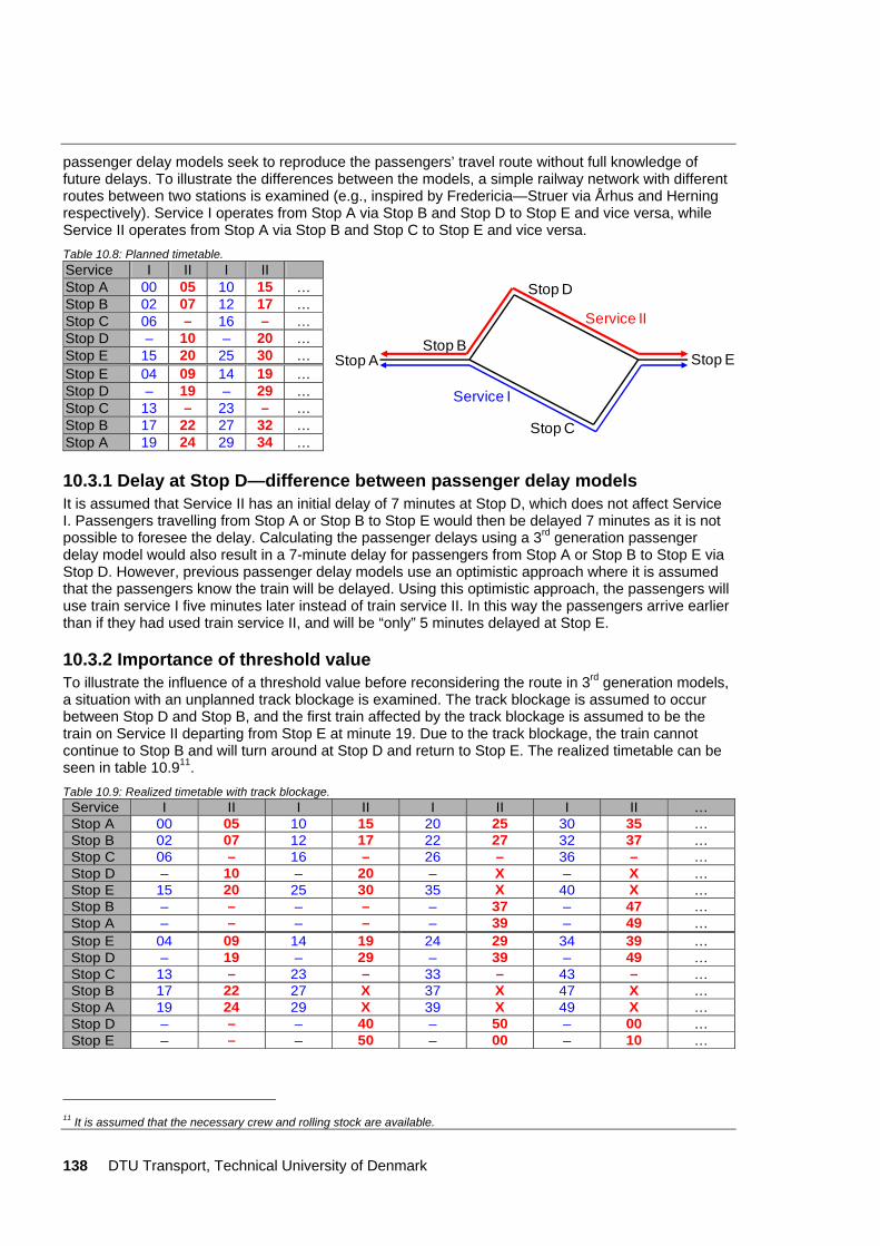
138 DTU Transport, Technical University of Denmark
passenger delay models seek to reproduce the passengers’ travel route without full knowledge of future delays. To illustrate the differences between the models, a simple railway network with different routes between two stations is examined (e.g., inspired by Fredericia—Struer via Århus and Herning respectively). Service I operates from Stop A via Stop B and Stop D to Stop E and vice versa, while Service II operates from Stop A via Stop B and Stop C to Stop E and vice versa. Table 10.8: Planned timetable. Service I II I II
Stop AStop B
Stop D
Stop C
Stop E
Service I
Service II
Stop A 00 05 10 15 … Stop B 02 07 12 17 … Stop C 06 – 16 – … Stop D – 10 – 20 … Stop E 15 20 25 30 … Stop E 04 09 14 19 … Stop D – 19 – 29 … Stop C 13 – 23 – … Stop B 17 22 27 32 … Stop A 19 24 29 34 …
10.3.1 Delay at Stop D—difference between passenger delay models It is assumed that Service II has an initial delay of 7 minutes at Stop D, which does not affect Service I. Passengers travelling from Stop A or Stop B to Stop E would then be delayed 7 minutes as it is not possible to foresee the delay. Calculating the passenger delays using a 3rd generation passenger delay model would also result in a 7-minute delay for passengers from Stop A or Stop B to Stop E via Stop D. However, previous passenger delay models use an optimistic approach where it is assumed that the passengers know the train will be delayed. Using this optimistic approach, the passengers will use train service I five minutes later instead of train service II. In this way the passengers arrive earlier than if they had used train service II, and will be “only” 5 minutes delayed at Stop E.
10.3.2 Importance of threshold value To illustrate the influence of a threshold value before reconsidering the route in 3rd generation models, a situation with an unplanned track blockage is examined. The track blockage is assumed to occur between Stop D and Stop B, and the first train affected by the track blockage is assumed to be the train on Service II departing from Stop E at minute 19. Due to the track blockage, the train cannot continue to Stop B and will turn around at Stop D and return to Stop E. The realized timetable can be seen in table 10.911. Table 10.9: Realized timetable with track blockage.
Service I II I II I II I II … Stop A 00 05 10 15 20 25 30 35 … Stop B 02 07 12 17 22 27 32 37 … Stop C 06 – 16 – 26 – 36 – … Stop D – 10 – 20 – X – X … Stop E 15 20 25 30 35 X 40 X … Stop B – – – – – 37 – 47 … Stop A – – – – – 39 – 49 … Stop E 04 09 14 19 24 29 34 39 … Stop D – 19 – 29 – 39 – 49 … Stop C 13 – 23 – 33 – 43 – … Stop B 17 22 27 X 37 X 47 X … Stop A 19 24 29 X 39 X 49 X … Stop D – – – 40 – 50 – 00 … Stop E – – – 50 – 00 – 10 …
11 It is assumed that the necessary crew and rolling stock are available.
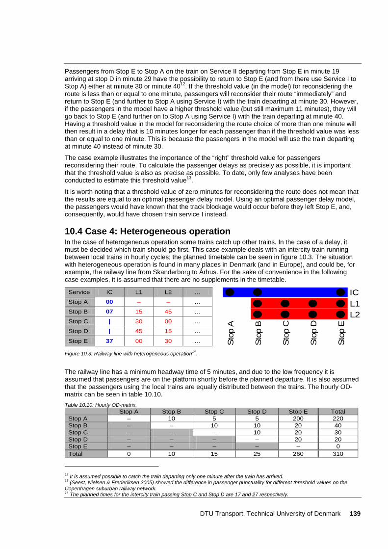
DTU Transport, Technical University of Denmark 139
Passengers from Stop E to Stop A on the train on Service II departing from Stop E in minute 19 arriving at stop D in minute 29 have the possibility to return to Stop E (and from there use Service I to Stop A) either at minute 30 or minute 4012. If the threshold value (in the model) for reconsidering the route is less than or equal to one minute, passengers will reconsider their route “immediately” and return to Stop E (and further to Stop A using Service I) with the train departing at minute 30. However, if the passengers in the model have a higher threshold value (but still maximum 11 minutes), they will go back to Stop E (and further on to Stop A using Service I) with the train departing at minute 40. Having a threshold value in the model for reconsidering the route choice of more than one minute will then result in a delay that is 10 minutes longer for each passenger than if the threshold value was less than or equal to one minute. This is because the passengers in the model will use the train departing at minute 40 instead of minute 30.
The case example illustrates the importance of the “right” threshold value for passengers reconsidering their route. To calculate the passenger delays as precisely as possible, it is important that the threshold value is also as precise as possible. To date, only few analyses have been conducted to estimate this threshold value13.
It is worth noting that a threshold value of zero minutes for reconsidering the route does not mean that the results are equal to an optimal passenger delay model. Using an optimal passenger delay model, the passengers would have known that the track blockage would occur before they left Stop E, and, consequently, would have chosen train service I instead.
10.4 Case 4: Heterogeneous operation In the case of heterogeneous operation some trains catch up other trains. In the case of a delay, it must be decided which train should go first. This case example deals with an intercity train running between local trains in hourly cycles; the planned timetable can be seen in figure 10.3. The situation with heterogeneous operation is found in many places in Denmark (and in Europe), and could be, for example, the railway line from Skanderborg to Århus. For the sake of convenience in the following case examples, it is assumed that there are no supplements in the timetable.
Service IC L1 L2 …
Sto
p A
Sto
p B
Sto
p C
Sto
p D
Sto
p E
ICL1L2
Stop A 00 – – …
Stop B 07 15 45 …
Stop C | 30 00 …
Stop D | 45 15 …
Stop E 37 00 30 … Figure 10.3: Railway line with heterogeneous operation14.
The railway line has a minimum headway time of 5 minutes, and due to the low frequency it is assumed that passengers are on the platform shortly before the planned departure. It is also assumed that the passengers using the local trains are equally distributed between the trains. The hourly OD-matrix can be seen in table 10.10. Table 10.10: Hourly OD-matrix.
Stop A Stop B Stop C Stop D Stop E Total Stop A – 10 5 5 200 220 Stop B – – 10 10 20 40 Stop C – – – 10 20 30 Stop D – – – – 20 20 Stop E – – – – – 0 Total 0 10 15 25 260 310
12 It is assumed possible to catch the train departing only one minute after the train has arrived. 13 (Seest, Nielsen & Frederiksen 2005) showed the difference in passenger punctuality for different threshold values on the Copenhagen suburban railway network. 14 The planned times for the intercity train passing Stop C and Stop D are 17 and 27 respectively.
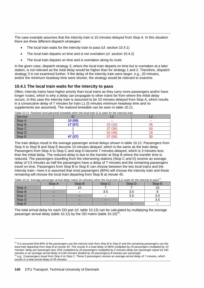
140 DTU Transport, Technical University of Denmark
The case example assumes that the intercity train is 10 minutes delayed from Stop A. In this situation there are three different dispatch strategies:
• The local train waits for the intercity train to pass (cf. section 10.4.1)
• The local train departs on time and is not overtaken (cf. section 10.4.2)
• The local train departs on time and is overtaken along its route
In the given case, dispatch strategy 3, where the local train departs on time but is overtaken at a later station, is not relevant as the total delay would be higher than for strategy 1 and 2. Therefore, dispatch strategy 3 is not examined further. If the delay of the intercity train were larger, e.g., 20 minutes, and/or the minimum headway time were shorter, the strategy would be relevant to examine.
10.4.1 The local train waits for the intercity to pass Often, intercity trains have higher priority than local trains as they carry more passengers and/or have longer routes, which is why a delay can propagate to other trains far from where the initial delay occurs. In this case the intercity train is assumed to be 10 minutes delayed from Stop A, which results in a consecutive delay of 7 minutes for train L1 (5 minutes minimum headway time and no supplements are assumed). The realized timetable can be seen in table 10.11. Table 10.11: Realized (and planned) timetable when the local train (L1) waits for the intercity train.
Service IC L1 L2 Stop A 10 (00) – – Stop B 17 (07) 22 (15) 45 Stop C | 37 (30) 00 Stop D | 52 (45) 15 Stop E 47 (37) 07 (00) 30
The train delays result in the average passenger arrival delays shown in table 10.12. Passengers from Stop A to Stop B and Stop E become 10 minutes delayed, which is the same as the train delay. Passengers from Stop A to Stop C and stop D become 7 minutes delayed, which is 3 minutes less than the initial delay. The reduced delay is due to the transfer at Stop B where the transfer time is reduced. The passengers travelling from the intervening stations (Stop C and D) receive an average delay of 3.5 minutes as half the passengers have a delay of 7 minutes and the remaining passengers travel on time. Passengers from Stop B to Stop E can choose between the two local trains and the intercity train—here it is assumed that most passengers (80%) will choose the intercity train and those remaining will choose the local train departing from Stop B at minute 45. Table 10.12: Average passenger arrival delay matrix (in minutes) when the local train (L1) waits for the intercity to pass15.
Stop A Stop B Stop C Stop D Stop E Stop A – 10 7 7 10 Stop B – – 3.5 3.5 8 Stop C – – – 3.5 3.5 Stop D – – – – 3.5 Stop E – – – – –
The total arrival delay for each OD-pair (cf. table 10.13) can be calculated by multiplying the average passenger arrival delay (table 10.12) by the OD matrix (table 10.10)16.
15 It is assumed that 80% of the passengers use the intercity train from Stop B to Stop E and the remaining passengers use the local train departing from Stop B at minute 45. This results in a total delay of (80% multiplied by 20 passengers multiplied by 10 minutes’ delay per passenger plus 20% multiplied by 20 passengers multiplied by 0 minutes delay per passenger equal to) 160 minutes or an average arrival delay of (160 minutes divided by 20 passengers) 8 minutes per passenger 16 e.g., 5 passengers travel from Stop A to Stop C. These 5 passengers receive an average arrival delay of 7 minutes, which results in a total arrival delay of 35 minutes.
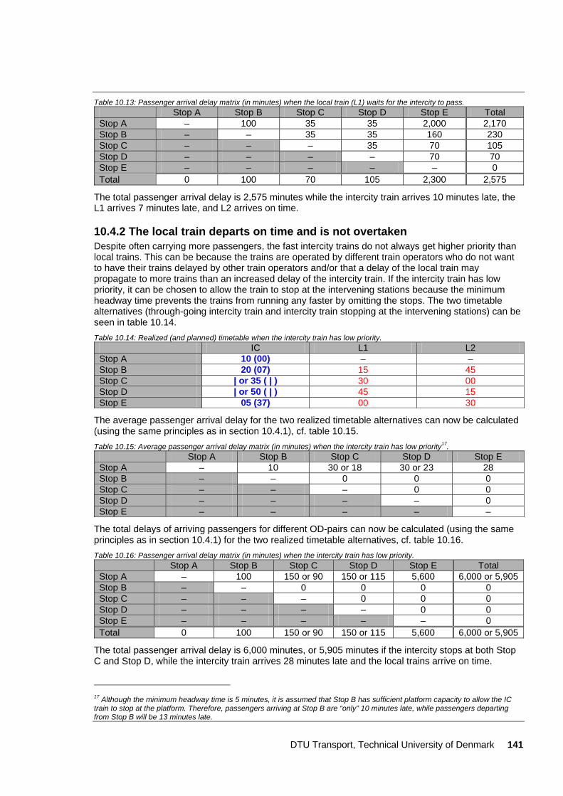
DTU Transport, Technical University of Denmark 141
Table 10.13: Passenger arrival delay matrix (in minutes) when the local train (L1) waits for the intercity to pass. Stop A Stop B Stop C Stop D Stop E Total Stop A – 100 35 35 2,000 2,170 Stop B – – 35 35 160 230 Stop C – – – 35 70 105 Stop D – – – – 70 70 Stop E – – – – – 0 Total 0 100 70 105 2,300 2,575
The total passenger arrival delay is 2,575 minutes while the intercity train arrives 10 minutes late, the L1 arrives 7 minutes late, and L2 arrives on time.
10.4.2 The local train departs on time and is not overtaken Despite often carrying more passengers, the fast intercity trains do not always get higher priority than local trains. This can be because the trains are operated by different train operators who do not want to have their trains delayed by other train operators and/or that a delay of the local train may propagate to more trains than an increased delay of the intercity train. If the intercity train has low priority, it can be chosen to allow the train to stop at the intervening stations because the minimum headway time prevents the trains from running any faster by omitting the stops. The two timetable alternatives (through-going intercity train and intercity train stopping at the intervening stations) can be seen in table 10.14. Table 10.14: Realized (and planned) timetable when the intercity train has low priority.
IC L1 L2 Stop A 10 (00) – – Stop B 20 (07) 15 45 Stop C | or 35 ( | ) 30 00 Stop D | or 50 ( | ) 45 15 Stop E 05 (37) 00 30
The average passenger arrival delay for the two realized timetable alternatives can now be calculated (using the same principles as in section 10.4.1), cf. table 10.15. Table 10.15: Average passenger arrival delay matrix (in minutes) when the intercity train has low priority17.
Stop A Stop B Stop C Stop D Stop E Stop A – 10 30 or 18 30 or 23 28 Stop B – – 0 0 0 Stop C – – – 0 0 Stop D – – – – 0 Stop E – – – – –
The total delays of arriving passengers for different OD-pairs can now be calculated (using the same principles as in section 10.4.1) for the two realized timetable alternatives, cf. table 10.16. Table 10.16: Passenger arrival delay matrix (in minutes) when the intercity train has low priority.
Stop A Stop B Stop C Stop D Stop E Total Stop A – 100 150 or 90 150 or 115 5,600 6,000 or 5,905 Stop B – – 0 0 0 0 Stop C – – – 0 0 0 Stop D – – – – 0 0 Stop E – – – – – 0 Total 0 100 150 or 90 150 or 115 5,600 6,000 or 5,905
The total passenger arrival delay is 6,000 minutes, or 5,905 minutes if the intercity stops at both Stop C and Stop D, while the intercity train arrives 28 minutes late and the local trains arrive on time.
17 Although the minimum headway time is 5 minutes, it is assumed that Stop B has sufficient platform capacity to allow the IC train to stop at the platform. Therefore, passengers arriving at Stop B are “only” 10 minutes late, while passengers departing from Stop B will be 13 minutes late.
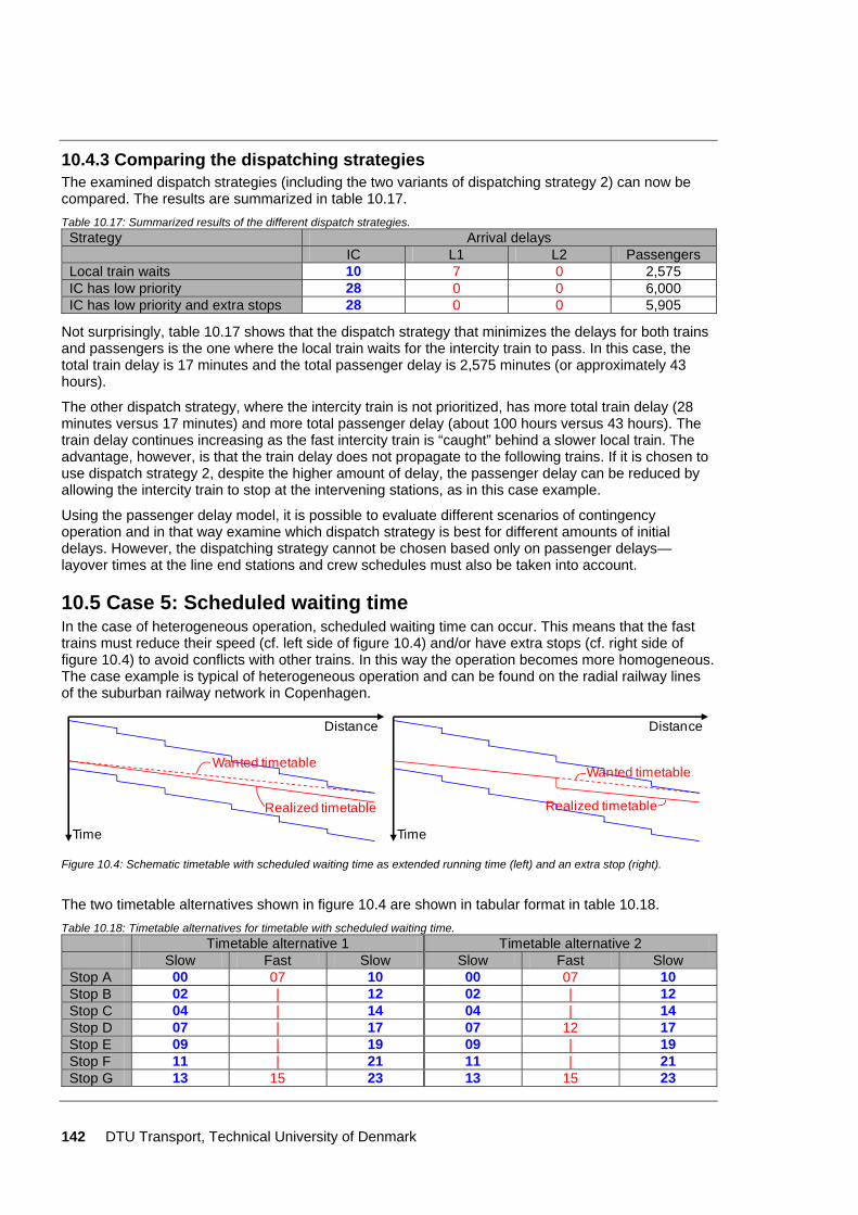
142 DTU Transport, Technical University of Denmark
10.4.3 Comparing the dispatching strategies The examined dispatch strategies (including the two variants of dispatching strategy 2) can now be compared. The results are summarized in table 10.17. Table 10.17: Summarized results of the different dispatch strategies.
Strategy Arrival delays IC L1 L2 Passengers Local train waits 10 7 0 2,575 IC has low priority 28 0 0 6,000 IC has low priority and extra stops 28 0 0 5,905
Not surprisingly, table 10.17 shows that the dispatch strategy that minimizes the delays for both trains and passengers is the one where the local train waits for the intercity train to pass. In this case, the total train delay is 17 minutes and the total passenger delay is 2,575 minutes (or approximately 43 hours).
The other dispatch strategy, where the intercity train is not prioritized, has more total train delay (28 minutes versus 17 minutes) and more total passenger delay (about 100 hours versus 43 hours). The train delay continues increasing as the fast intercity train is “caught” behind a slower local train. The advantage, however, is that the train delay does not propagate to the following trains. If it is chosen to use dispatch strategy 2, despite the higher amount of delay, the passenger delay can be reduced by allowing the intercity train to stop at the intervening stations, as in this case example.
Using the passenger delay model, it is possible to evaluate different scenarios of contingency operation and in that way examine which dispatch strategy is best for different amounts of initial delays. However, the dispatching strategy cannot be chosen based only on passenger delays—layover times at the line end stations and crew schedules must also be taken into account.
10.5 Case 5: Scheduled waiting time In the case of heterogeneous operation, scheduled waiting time can occur. This means that the fast trains must reduce their speed (cf. left side of figure 10.4) and/or have extra stops (cf. right side of figure 10.4) to avoid conflicts with other trains. In this way the operation becomes more homogeneous. The case example is typical of heterogeneous operation and can be found on the radial railway lines of the suburban railway network in Copenhagen.
Time
Distance
Time
Distance
Wanted timetable
Realized timetable Realized timetable
Wanted timetable
Figure 10.4: Schematic timetable with scheduled waiting time as extended running time (left) and an extra stop (right).
The two timetable alternatives shown in figure 10.4 are shown in tabular format in table 10.18. Table 10.18: Timetable alternatives for timetable with scheduled waiting time.
Timetable alternative 1 Timetable alternative 2 Slow Fast Slow Slow Fast Slow Stop A 00 07 10 00 07 10 Stop B 02 | 12 02 | 12 Stop C 04 | 14 04 | 14 Stop D 07 | 17 07 12 17 Stop E 09 | 19 09 | 19 Stop F 11 | 21 11 | 21 Stop G 13 15 23 13 15 23
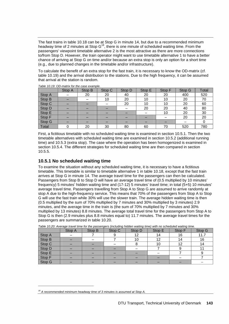
DTU Transport, Technical University of Denmark 143
The fast trains in table 10.18 can be at Stop G in minute 14, but due to a recommended minimum headway time of 2 minutes at Stop G18, there is one minute of scheduled waiting time. From the passengers’ viewpoint timetable alternative 2 is the most attractive as there are more connections to/from Stop D. However, the train operator might want to use timetable alternative 1 to have a better chance of arriving at Stop G on time and/or because an extra stop is only an option for a short time (e.g., due to planned changes in the timetable and/or infrastructure).
To calculate the benefit of an extra stop for the fast train, it is necessary to know the OD-matrix (cf. table 10.19) and the arrival distribution to the stations. Due to the high frequency, it can be assumed that arrival at the station is random. Table 10.19: OD-matrix for the case example.
Stop A Stop B Stop C Stop D Stop E Stop F Stop G Total Stop A – 20 20 40 20 20 400 520 Stop B – – 10 20 10 10 20 70 Stop C – – – 20 10 10 20 60 Stop D – – – – 20 20 40 80 Stop E – – – – – 10 20 30 Stop F – – – – – – 20 20 Stop G – – – – – – – 0 Total 0 20 30 80 60 70 520 780
First, a fictitious timetable with no scheduled waiting time is examined in section 10.5.1. Then the two timetable alternatives with scheduled waiting time are examined in section 10.5.2 (additional running time) and 10.5.3 (extra stop). The case where the operation has been homogenized is examined in section 10.5.4. The different strategies for scheduled waiting time are then compared in section 10.5.5.
10.5.1 No scheduled waiting time To examine the situation without any scheduled waiting time, it is necessary to have a fictitious timetable. This timetable is similar to timetable alternative 1 in table 10.18, except that the fast train arrives at Stop G in minute 14. The average travel time for the passengers can then be calculated. Passengers from Stop B to Stop D will have an average travel time of (0.5 multiplied by 10 minutes’ frequency) 5 minutes’ hidden waiting time and (17-12) 5 minutes’ travel time; in total (5+5) 10 minutes’ average travel time. Passengers travelling from Stop A to Stop G are assumed to arrive randomly at stop A due to the high-frequency service. This means that 70% of the passengers from Stop A to Stop G will use the fast train while 30% will use the slower train. The average hidden waiting time is then (0.5 multiplied by the sum of 70% multiplied by 7 minutes and 30% multiplied by 3 minutes) 2.9 minutes, and the average time in the train is (the sum of 70% multiplied by 7 minutes and 30% multiplied by 13 minutes) 8.8 minutes. The average total travel time for the passengers from Stop A to Stop G is then (2.9 minutes plus 8.8 minutes equal to) 11.7 minutes. The average travel times for the passengers are summarized in table 10.20. Table 10.20: Average travel time for the passengers (including hidden waiting time) with no scheduled waiting time.
Stop A Stop B Stop C Stop D Stop E Stop F Stop G Stop A – 7 9 12 14 16 11.7 Stop B – – 7 10 12 14 16 Stop C – – – 8 10 12 14 Stop D – – – – 7 9 11 Stop E – – – – – 7 9 Stop F – – – – – – 7 Stop G – – – – – – –
18 A recommended minimum headway time of 3 minutes is assumed at Stop A.
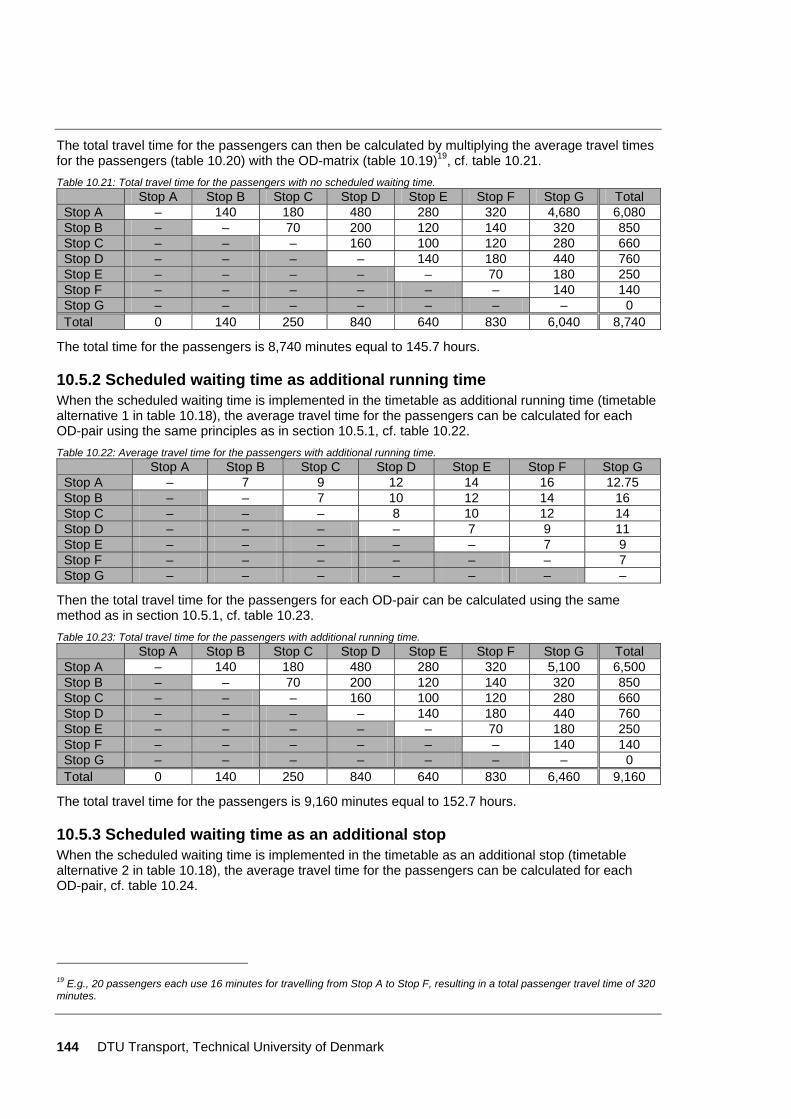
144 DTU Transport, Technical University of Denmark
The total travel time for the passengers can then be calculated by multiplying the average travel times for the passengers (table 10.20) with the OD-matrix (table 10.19)19, cf. table 10.21. Table 10.21: Total travel time for the passengers with no scheduled waiting time.
Stop A Stop B Stop C Stop D Stop E Stop F Stop G Total Stop A – 140 180 480 280 320 4,680 6,080 Stop B – – 70 200 120 140 320 850 Stop C – – – 160 100 120 280 660 Stop D – – – – 140 180 440 760 Stop E – – – – – 70 180 250 Stop F – – – – – – 140 140 Stop G – – – – – – – 0 Total 0 140 250 840 640 830 6,040 8,740
The total time for the passengers is 8,740 minutes equal to 145.7 hours.
10.5.2 Scheduled waiting time as additional running time When the scheduled waiting time is implemented in the timetable as additional running time (timetable alternative 1 in table 10.18), the average travel time for the passengers can be calculated for each OD-pair using the same principles as in section 10.5.1, cf. table 10.22. Table 10.22: Average travel time for the passengers with additional running time.
Stop A Stop B Stop C Stop D Stop E Stop F Stop G Stop A – 7 9 12 14 16 12.75 Stop B – – 7 10 12 14 16 Stop C – – – 8 10 12 14 Stop D – – – – 7 9 11 Stop E – – – – – 7 9 Stop F – – – – – – 7 Stop G – – – – – – –
Then the total travel time for the passengers for each OD-pair can be calculated using the same method as in section 10.5.1, cf. table 10.23. Table 10.23: Total travel time for the passengers with additional running time.
Stop A Stop B Stop C Stop D Stop E Stop F Stop G Total Stop A – 140 180 480 280 320 5,100 6,500 Stop B – – 70 200 120 140 320 850 Stop C – – – 160 100 120 280 660 Stop D – – – – 140 180 440 760 Stop E – – – – – 70 180 250 Stop F – – – – – – 140 140 Stop G – – – – – – – 0 Total 0 140 250 840 640 830 6,460 9,160
The total travel time for the passengers is 9,160 minutes equal to 152.7 hours.
10.5.3 Scheduled waiting time as an additional stop When the scheduled waiting time is implemented in the timetable as an additional stop (timetable alternative 2 in table 10.18), the average travel time for the passengers can be calculated for each OD-pair, cf. table 10.24.
19 E.g., 20 passengers each use 16 minutes for travelling from Stop A to Stop F, resulting in a total passenger travel time of 320 minutes.
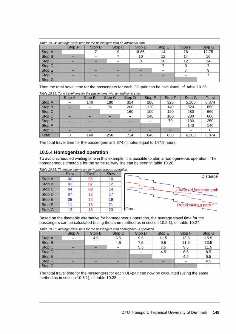
DTU Transport, Technical University of Denmark 145
Table 10.24: Average travel time for the passengers with an additional stop. Stop A Stop B Stop C Stop D Stop E Stop F Stop G Stop A – 7 9 8.85 14 16 12.75 Stop B – – 7 10 12 14 16 Stop C – – – 8 10 12 14 Stop D – – – – 7 9 7 Stop E – – – – – 7 9 Stop F – – – – – – 7 Stop G – – – – – – –
Then the total travel time for the passengers for each OD-pair can be calculated, cf. table 10.25. Table 10.25: Total travel time for the passengers with an additional stop.
Stop A Stop B Stop C Stop D Stop E Stop F Stop G Total Stop A – 140 180 354 280 320 5,100 6,374 Stop B – – 70 200 120 140 320 850 Stop C – – – 160 100 120 280 660 Stop D – – – – 140 180 280 600 Stop E – – – – – 70 180 250 Stop F – – – – – – 140 140 Stop G – – – – – – – 0 Total 0 140 250 714 640 830 6,300 8,874
The total travel time for the passengers is 8,874 minutes equal to 147.9 hours.
10.5.4 Homogenized operation To avoid scheduled waiting time in this example, it is possible to plan a homogeneous operation. The homogeneous timetable for the same railway line can be seen in table 10.26. Table 10.26: Timetable alternative for homogeneous operation.
Slow “Fast” Slow
Time
Distance
Wanted fast train path
Realized train path
Stop A 00 05 10 Stop B 02 07 12 Stop C 04 09 14 Stop D 07 12 17 Stop E 09 14 19 Stop F 11 16 21 Stop G 13 18 23
Based on the timetable alternative for homogeneous operation, the average travel time for the passengers can be calculated (using the same method as in section 10.5.1), cf. table 10.27. Table 10.27: Average travel time for the passengers with homogeneous operation.
Stop A Stop B Stop C Stop D Stop E Stop F Stop G Stop A – 4.5 6.5 9.5 11.5 13.5 15.5 Stop B – – 4.5 7.5 9.5 11.5 13.5 Stop C – – – 5.5 7.5 9.5 11.5 Stop D – – – – 4.5 6.5 8.5 Stop E – – – – – 4.5 6.5 Stop F – – – – – – 4.5 Stop G – – – – – – –
The total travel time for the passengers for each OD-pair can now be calculated (using the same method as in section 10.5.1), cf. table 10.28.
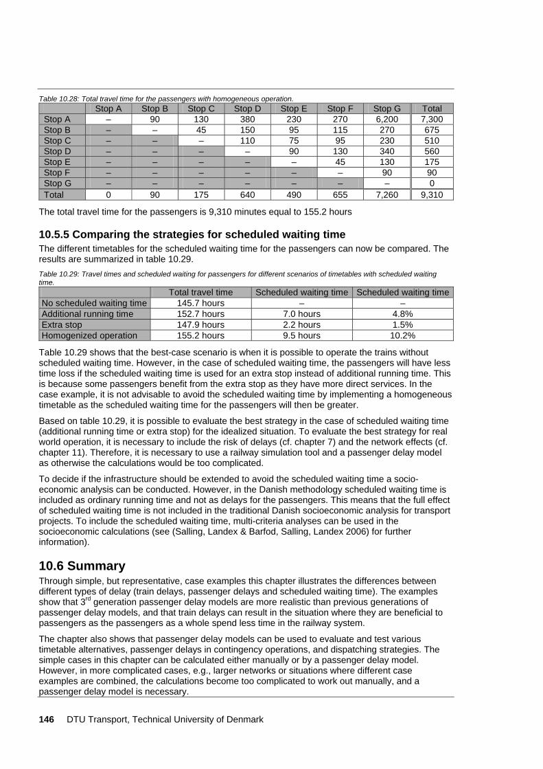
146 DTU Transport, Technical University of Denmark
Table 10.28: Total travel time for the passengers with homogeneous operation. Stop A Stop B Stop C Stop D Stop E Stop F Stop G Total Stop A – 90 130 380 230 270 6,200 7,300 Stop B – – 45 150 95 115 270 675 Stop C – – – 110 75 95 230 510 Stop D – – – – 90 130 340 560 Stop E – – – – – 45 130 175 Stop F – – – – – – 90 90 Stop G – – – – – – – 0 Total 0 90 175 640 490 655 7,260 9,310
The total travel time for the passengers is 9,310 minutes equal to 155.2 hours
10.5.5 Comparing the strategies for scheduled waiting time The different timetables for the scheduled waiting time for the passengers can now be compared. The results are summarized in table 10.29. Table 10.29: Travel times and scheduled waiting for passengers for different scenarios of timetables with scheduled waiting time. Total travel time Scheduled waiting time Scheduled waiting timeNo scheduled waiting time 145.7 hours – – Additional running time 152.7 hours 7.0 hours 4.8% Extra stop 147.9 hours 2.2 hours 1.5% Homogenized operation 155.2 hours 9.5 hours 10.2%
Table 10.29 shows that the best-case scenario is when it is possible to operate the trains without scheduled waiting time. However, in the case of scheduled waiting time, the passengers will have less time loss if the scheduled waiting time is used for an extra stop instead of additional running time. This is because some passengers benefit from the extra stop as they have more direct services. In the case example, it is not advisable to avoid the scheduled waiting time by implementing a homogeneous timetable as the scheduled waiting time for the passengers will then be greater.
Based on table 10.29, it is possible to evaluate the best strategy in the case of scheduled waiting time (additional running time or extra stop) for the idealized situation. To evaluate the best strategy for real world operation, it is necessary to include the risk of delays (cf. chapter 7) and the network effects (cf. chapter 11). Therefore, it is necessary to use a railway simulation tool and a passenger delay model as otherwise the calculations would be too complicated.
To decide if the infrastructure should be extended to avoid the scheduled waiting time a socio-economic analysis can be conducted. However, in the Danish methodology scheduled waiting time is included as ordinary running time and not as delays for the passengers. This means that the full effect of scheduled waiting time is not included in the traditional Danish socioeconomic analysis for transport projects. To include the scheduled waiting time, multi-criteria analyses can be used in the socioeconomic calculations (see (Salling, Landex & Barfod, Salling, Landex 2006) for further information).
10.6 Summary Through simple, but representative, case examples this chapter illustrates the differences between different types of delay (train delays, passenger delays and scheduled waiting time). The examples show that 3rd generation passenger delay models are more realistic than previous generations of passenger delay models, and that train delays can result in the situation where they are beneficial to passengers as the passengers as a whole spend less time in the railway system.
The chapter also shows that passenger delay models can be used to evaluate and test various timetable alternatives, passenger delays in contingency operations, and dispatching strategies. The simple cases in this chapter can be calculated either manually or by a passenger delay model. However, in more complicated cases, e.g., larger networks or situations where different case examples are combined, the calculations become too complicated to work out manually, and a passenger delay model is necessary.
DTU Transport, Technical University of Denmark 147
Chapter 11
11 Network effects Railway operation is affected by network effects: a change in one part of the network can influence other parts of the network. This influence can be far from where the original change was made, hence the term network effects. Network effects occur because train services are often relatively long and because the railway system has a high degree of interdependencies as trains cannot cross each other or overtake each other everywhere in the network.
Network effects can be defined as the interdependencies between the railway lines in a network and the interaction between the trains operated in the network. This means that additional dwell time at a transfer station to achieve good transfers for the passengers can be considered as a network effect. Additional supplements in the timetable and extra running time for the trains because of other trains in the network and other departure times than originally wanted are, too, network effects. Furthermore, crew scheduling and rostering of train units can result in additional network effects. It can be argued that each time a choice regarding the timetable is taken the choice affects the goodness/attractiveness of the timetable. Therefore, it is necessary to include the entire network and its timetable when examining the network effects (e.g., using micro-simulation tools).
Although the risk of network effects is known, many analysis/projects (at least in Denmark1) only investigate the effects of changed timetables and/or infrastructure locally or for a smaller part of the network. This can be due to lack of resources (time and/or money), or because the network effects are considered uncertain or insignificant, or because it is wished to evaluate the project only locally, isolated from the remaining network. It is particularly important to examine the network effects in the case of high capacity consumption in the railway network because it is here the most network effects can be expected.
Network effects are dependent on the given infrastructure and timetable (including train allocations) and can result in longer travel times for trains and passengers. Passengers can be further affected by the network effects if the wanted transfers to/from other trains cannot be kept due to too many interdependencies—or network effects. Furthermore, the network effects can result in reduced capacity as some trains or train services may make it impossible to operate other planned/desired trains or train services.
As figure 11.1 indicates, there are several interconnected bottlenecks in the Danish railway system. Some of these may be “hidden” to the users, since they are considered and dealt with in the timetable planning process (whereby the timetables becomes less attractive than the passenger demand would justify). However, network effects may still occur in the operation where they can influence trains and/or passengers.
Although networks effects are generally recognized and understood by practitioners in rail companies, many project appraisals in the rail sector consider only a sub-set of the network, for example, the line in question, whereby possible network effects are overlooked. One reason for this is the increasing calculation complexity if network effects for the entire network are to be analysed. Another is that the economists and planners who do the project appraisal may not be experts in rail capacity issues.
First, this chapter presents the network effects in general (section 11.1). This is followed by descriptions of the four kinds of network effects: network effects in the train schedule planning process (section 11.2), network effects for trains and passengers (section 11.3), and network effects for contingency operation (section 11.4). Then, section 11.5 describes how network effects can be quantified by scheduled waiting time. Before summing up in section 11.7, section 11.6 discusses how network effects can be used to prioritize different improvements of the infrastructure.
1 For example, several of the analyses on double track between Lejre and Vipperød, e.g., (National Rail Authority 2007a).
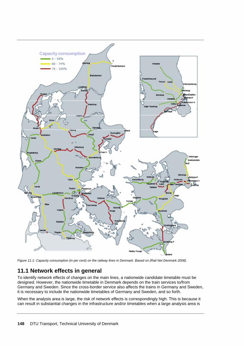
148 DTU Transport, Technical University of Denmark
Capacity consumption
Figure 11.1: Capacity consumption (in per cent) on the railway lines in Denmark. Based on (Rail Net Denmark 2008).
11.1 Network effects in general To identify network effects of changes on the main lines, a nationwide candidate timetable must be designed. However, the nationwide timetable in Denmark depends on the train services to/from Germany and Sweden. Since the cross-border service also affects the trains in Germany and Sweden, it is necessary to include the nationwide timetables of Germany and Sweden, and so forth.
When the analysis area is large, the risk of network effects is correspondingly high. This is because it can result in substantial changes in the infrastructure and/or timetables when a large analysis area is

DTU Transport, Technical University of Denmark 149
examined. Major changes in the infrastructure and/or timetables may influence many trains in the analysis area, and these trains may in turn influence other trains outside the analysis area.
However, even smaller analysis areas may generate network effects. This is due to the way of planning the timetable in Denmark and many other countries. All train services can be placed in a ranked order where trains with fast, long distance services are planned and timetabled before trains with slower, short distances.
Although the ranked order of planning national passenger trains is straightforward, the international passenger trains and freight trains complicate it. The international passenger trains are normally not the backbone of the national timetable, which is why these trains have to be “fitted” into the timetable without obstructing its structure. Freight trains are often given a relatively low priority and should, therefore, be located at the bottom of the hierarchy. However, freight trains are often long distance trains operated on the main lines and some freight trains may have high priority. Therefore, it is necessary to consider the freight trains when scheduling other trains. The ranked order of planning the train services is shown in figure 11.2.
Intercity Express
Intercity
Regional
Local
International Interregional Freight
Figure 11.2: Ranked order of planning train services. Inspired by (Hansen, Landex & Kaas 2006, Landex, Kaas & Hansen 2006).
Even small changes in the timetable of a train of the first planned trains may influence later planned trains as these trains are planned according to the first planned trains. Since the first planned trains often travel long distances, the changes for other train services can occur far from the analysis area.
EXAMPLE An example to illustrate how a change of the first planned train services can affect trains far away in the network is the Danish railway line between Aalborg and Frederikshavn, cf. figure 11.3, left side. It is a single-track line with an hourly service with a maximum speed of 120 km/h. The travel time in one direction is 63 minutes and 66 minutes in the other direction (Hansen 2004b).
A project of increasing the speed from 120 km/h to 180 km/h is now examined. This project can be evaluated locally. However, the traffic in the northern part of Denmark is not timetabled independently of the remaining network. The trains are part of the nationwide intercity system (cf. figure 11.3, right side) and are, therefore, adapted to the arrival and departure times of the IC-trains at Aalborg (as well as the crossing possibilities in the northern part of Denmark).
If the crossing station in the candidate timetable for the upgrading project is changed, it may influence the trains, as they have to speed up/slow down to obtain the new crossings. The obtained time benefits (e.g. 10 minutes for one of the directions) can be analysed locally. However, as a change in the northern part of Denmark will influence the IC-trains, the nationwide timetable will be influenced too.
This is because most regional trains have planned transfer(s) to and from IC-trains. Therefore, the regional trains between Copenhagen/Ringsted and Nykøbing F (in the south-eastern part of Denmark) might be influenced too as there is a planned transfer at Ringsted, cf. figure 11.3. Therefore, the change in the northern part of Denmark may well result in time benefits (or losses) on other railway lines in the network.
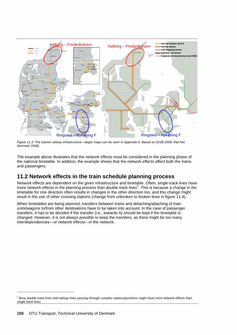
150 DTU Transport, Technical University of Denmark
Intercity Express serviceIntercity serviceDSB Regional serviceSuburban rail serviceRegional and local services (not DSB)
Intercity Express serviceIntercity serviceDSB Regional serviceSuburban rail serviceRegional and local services (not DSB)
Aalborg – Frederikshavn Aalborg – Frederikshavn
Ringsted – Nykøbing F Ringsted – Nykøbing F Figure 11.3: The Danish railway infrastructure—larger maps can be seen in Appendix 6. Based on (DSB 2008, Rail Net Denmark 2008).
The example above illustrates that the network effects must be considered in the planning phase of the national timetable. In addition, the example shows that the network effects affect both the trains and passengers.
11.2 Network effects in the train schedule planning process Network effects are dependent on the given infrastructure and timetable. Often, single-track lines have more network effects in the planning process than double track lines2. This is because a change in the timetable for one direction often results in changes in the other direction too, and this change might result in the use of other crossing stations (change from unbroken to broken lines in figure 11.4).
When timetables are being planned, transfers between trains and detaching/attaching of train units/wagons to/from other destinations have to be taken into account. In the case of passenger transfers, it has to be decided if the transfer (i.e., towards A) should be kept if the timetable is changed. However, it is not always possible to keep the transfers, as there might be too many interdependencies—or network effects—in the network.
2 Busy double track lines and railway lines passing through complex stations/junctions might have more network effects than single track lines.
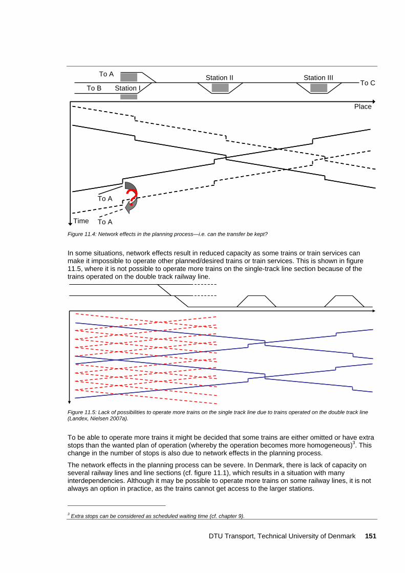
DTU Transport, Technical University of Denmark 151
To A
To A
To A
?
To BTo C
Place
Time
Station IStation II Station III
Figure 11.4: Network effects in the planning process—i.e. can the transfer be kept?
In some situations, network effects result in reduced capacity as some trains or train services can make it impossible to operate other planned/desired trains or train services. This is shown in figure 11.5, where it is not possible to operate more trains on the single-track line section because of the trains operated on the double track railway line.
Figure 11.5: Lack of possibilities to operate more trains on the single track line due to trains operated on the double track line (Landex, Nielsen 2007a).
To be able to operate more trains it might be decided that some trains are either omitted or have extra stops than the wanted plan of operation (whereby the operation becomes more homogeneous)3. This change in the number of stops is also due to network effects in the planning process.
The network effects in the planning process can be severe. In Denmark, there is lack of capacity on several railway lines and line sections (cf. figure 11.1), which results in a situation with many interdependencies. Although it may be possible to operate more trains on some railway lines, it is not always an option in practice, as the trains cannot get access to the larger stations.
3 Extra stops can be considered as scheduled waiting time (cf. chapter 9).
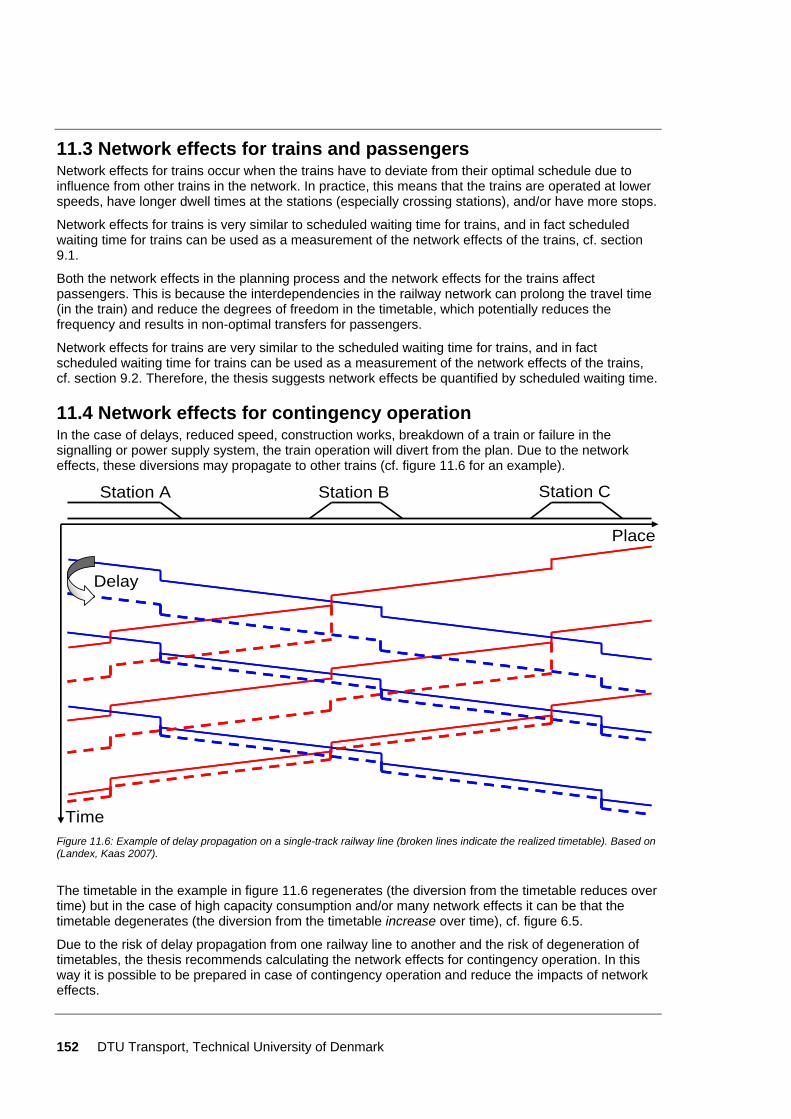
152 DTU Transport, Technical University of Denmark
11.3 Network effects for trains and passengers Network effects for trains occur when the trains have to deviate from their optimal schedule due to influence from other trains in the network. In practice, this means that the trains are operated at lower speeds, have longer dwell times at the stations (especially crossing stations), and/or have more stops.
Network effects for trains is very similar to scheduled waiting time for trains, and in fact scheduled waiting time for trains can be used as a measurement of the network effects of the trains, cf. section 9.1.
Both the network effects in the planning process and the network effects for the trains affect passengers. This is because the interdependencies in the railway network can prolong the travel time (in the train) and reduce the degrees of freedom in the timetable, which potentially reduces the frequency and results in non-optimal transfers for passengers.
Network effects for trains are very similar to the scheduled waiting time for trains, and in fact scheduled waiting time for trains can be used as a measurement of the network effects of the trains, cf. section 9.2. Therefore, the thesis suggests network effects be quantified by scheduled waiting time.
11.4 Network effects for contingency operation In the case of delays, reduced speed, construction works, breakdown of a train or failure in the signalling or power supply system, the train operation will divert from the plan. Due to the network effects, these diversions may propagate to other trains (cf. figure 11.6 for an example).
Place
Time
Station A Station B Station C
Delay
Figure 11.6: Example of delay propagation on a single-track railway line (broken lines indicate the realized timetable). Based on (Landex, Kaas 2007).
The timetable in the example in figure 11.6 regenerates (the diversion from the timetable reduces over time) but in the case of high capacity consumption and/or many network effects it can be that the timetable degenerates (the diversion from the timetable increase over time), cf. figure 6.5.
Due to the risk of delay propagation from one railway line to another and the risk of degeneration of timetables, the thesis recommends calculating the network effects for contingency operation. In this way it is possible to be prepared in case of contingency operation and reduce the impacts of network effects.
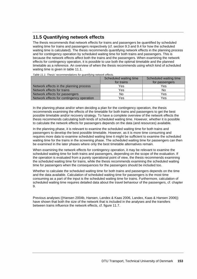
DTU Transport, Technical University of Denmark 153
11.5 Quantifying network effects The thesis recommends that network effects for trains and passengers be quantified by scheduled waiting time for trains and passengers respectively (cf. section 9.3 and 9.4 for how the scheduled waiting time is calculated). The thesis recommends quantifying network effects in the planning process and for contingency operation by scheduled waiting time for both trains and passengers. This is because the network effects affect both the trains and the passengers. When examining the network effects for contingency operation, it is possible to use both the optimal timetable and the planned timetable as a reference. An overview of when the thesis recommends using which kind of scheduled waiting time is given in table 11.1. Table 11.1: Thesis’ recommendations for quantifying network effects. Scheduled waiting time
for trains Scheduled waiting time
for passengers Network effects in the planning process Yes Yes Network effects for trains Yes No Network effects for passengers No Yes Network effects for contingency operation Yes Yes
In the planning phase and/or when deciding a plan for the contingency operation, the thesis recommends examining the effects of the timetable for both trains and passengers to get the best possible timetable and/or recovery strategy. To have a complete overview of the network effects the thesis recommends calculating both kinds of scheduled waiting time. However, whether it is possible to calculate the network effects for passengers depends on the data (and resources) available.
In the planning phase, it is relevant to examine the scheduled waiting time for both trains and passengers to develop the best possible timetable. However, as it is more time consuming and requires more data to examine scheduled waiting time it might be sufficient to examine the scheduled waiting time for the trains in the screening phase. The scheduled waiting time for passengers can then be examined in the later phases where only the best timetable alternatives remain.
When examining the network effects for contingency operation, it may be relevant to examine the scheduled waiting time for both trains and passengers, depending on the scope of the evaluation. If the operation is evaluated from a purely operational point of view, the thesis recommends examining the scheduled waiting time for trains, while the thesis recommends examining the scheduled waiting time for passengers when the consequences for the passengers should be included too.
Whether to calculate the scheduled waiting time for both trains and passengers depends on the time and the data available. Calculation of scheduled waiting time for passengers is the most time consuming as a part of the input is the scheduled waiting time for trains. Furthermore, calculation of scheduled waiting time requires detailed data about the travel behaviour of the passengers, cf. chapter 9.
Previous analyses ((Hansen 2004b, Hansen, Landex & Kaas 2006, Landex, Kaas & Hansen 2006)) have shown that both the size of the network that is included in the analyses and the transfers between trains influence the network effects, cf. figure 11.7.
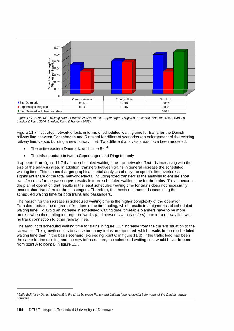
154 DTU Transport, Technical University of Denmark
0
0.01
0.02
0.03
0.04
0.05
0.06
0.07
Current situation Enlarged line New lineEast Denmark 0.042 0.048 0.057Copenhagen-Ringsted 0.033 0.046 0.033East Denmark with fixed transfers 0.061
Sche
dule
d w
aitin
g tim
eM
inut
es p
er tr
ain-
km
Figure 11.7: Scheduled waiting time for trains/Network effects Copenhagen-Ringsted. Based on (Hansen 2004b, Hansen, Landex & Kaas 2006, Landex, Kaas & Hansen 2006).
Figure 11.7 illustrates network effects in terms of scheduled waiting time for trains for the Danish railway line between Copenhagen and Ringsted for different scenarios (an enlargement of the existing railway line, versus building a new railway line). Two different analysis areas have been modelled:
• The entire eastern Denmark, until Little Belt4
• The infrastructure between Copenhagen and Ringsted only
It appears from figure 11.7 that the scheduled waiting time—or network effect—is increasing with the size of the analysis area. In addition, transfers between trains in general increase the scheduled waiting time. This means that geographical partial analyses of only the specific line overlook a significant share of the total network effects. Including fixed transfers in the analysis to ensure short transfer times for the passengers results in more scheduled waiting time for the trains. This is because the plan of operation that results in the least scheduled waiting time for trains does not necessarily ensure short transfers for the passengers. Therefore, the thesis recommends examining the scheduled waiting time for both trains and passengers.
The reason for the increase in scheduled waiting time is the higher complexity of the operation. Transfers reduce the degree of freedom in the timetabling, which results in a higher risk of scheduled waiting time. To avoid an increase in scheduled waiting time, timetable planners have to be more precise when timetabling for larger networks (and networks with transfers) than for a railway line with no track connection to other railway lines.
The amount of scheduled waiting time for trains in figure 11.7 increase from the current situation to the scenarios. This growth occurs because too many trains are operated, which results in more scheduled waiting time than in the basis scenario (exceeding point C in figure 11.8). If the traffic load had been the same for the existing and the new infrastructure, the scheduled waiting time would have dropped from point A to point B in figure 11.8.
4 Little Belt (or in Danish Lillebælt) is the strait between Funen and Jutland (see Appendix 6 for maps of the Danish railway network).
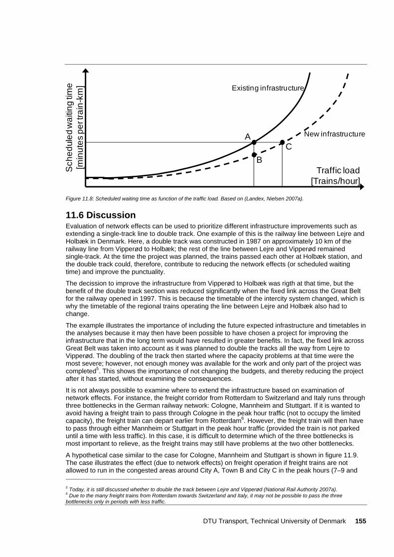
DTU Transport, Technical University of Denmark 155
Traffic load[Trains/hour]
Sch
edul
ed w
aitin
g tim
e[m
inut
es p
er tr
ain-
km] Existing infrastructure
New infrastructure
CA
B
Figure 11.8: Scheduled waiting time as function of the traffic load. Based on (Landex, Nielsen 2007a).
11.6 Discussion Evaluation of network effects can be used to prioritize different infrastructure improvements such as extending a single-track line to double track. One example of this is the railway line between Lejre and Holbæk in Denmark. Here, a double track was constructed in 1987 on approximately 10 km of the railway line from Vipperød to Holbæk; the rest of the line between Lejre and Vipperød remained single-track. At the time the project was planned, the trains passed each other at Holbæk station, and the double track could, therefore, contribute to reducing the network effects (or scheduled waiting time) and improve the punctuality.
The decission to improve the infrastructure from Vipperød to Holbæk was rigth at that time, but the benefit of the double track section was reduced significantly when the fixed link across the Great Belt for the railway opened in 1997. This is because the timetable of the intercity system changed, which is why the timetable of the regional trains operating the line between Lejre and Holbæk also had to change.
The example illustrates the importance of including the future expected infrastructure and timetables in the analyses because it may then have been possible to have chosen a project for improving the infrastructure that in the long term would have resulted in greater benefits. In fact, the fixed link across Great Belt was taken into account as it was planned to double the tracks all the way from Lejre to Vipperød. The doubling of the track then started where the capacity problems at that time were the most severe; however, not enough money was available for the work and only part of the project was completed5. This shows the importance of not changing the budgets, and thereby reducing the project after it has started, without examining the consequences.
It is not always possible to examine where to extend the infrastructure based on examination of network effects. For instance, the freight corridor from Rotterdam to Switzerland and Italy runs through three bottlenecks in the German railway network: Cologne, Mannheim and Stuttgart. If it is wanted to avoid having a freight train to pass through Cologne in the peak hour traffic (not to occupy the limited capacity), the freight train can depart earlier from Rotterdam6. However, the freight train will then have to pass through either Mannheim or Stuttgart in the peak hour traffic (provided the train is not parked until a time with less traffic). In this case, it is difficult to determine which of the three bottlenecks is most important to relieve, as the freight trains may still have problems at the two other bottlenecks.
A hypothetical case similar to the case for Cologne, Mannheim and Stuttgart is shown in figure 11.9. The case illustrates the effect (due to network effects) on freight operation if freight trains are not allowed to run in the congested areas around City A, Town B and City C in the peak hours (7–9 and 5 Today, it is still discussed whether to double the track between Lejre and Vipperød (National Rail Authority 2007a). 6 Due to the many freight trains from Rotterdam towards Switzerland and Italy, it may not be possible to pass the three bottlenecks only in periods with less traffic.
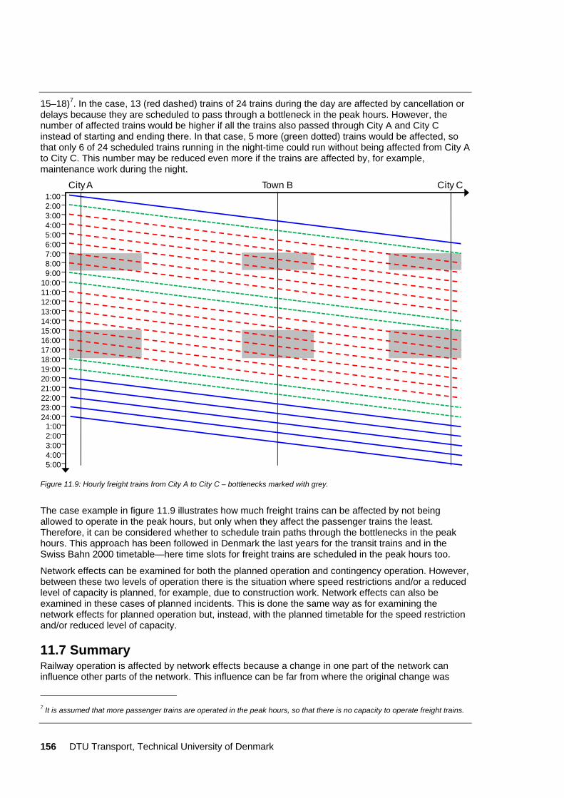
156 DTU Transport, Technical University of Denmark
15–18)7. In the case, 13 (red dashed) trains of 24 trains during the day are affected by cancellation or delays because they are scheduled to pass through a bottleneck in the peak hours. However, the number of affected trains would be higher if all the trains also passed through City A and City C instead of starting and ending there. In that case, 5 more (green dotted) trains would be affected, so that only 6 of 24 scheduled trains running in the night-time could run without being affected from City A to City C. This number may be reduced even more if the trains are affected by, for example, maintenance work during the night.
5:006:007:008:009:00
10:0011:0012:0013:0014:0015:0016:0017:0018:0019:0020:0021:0022:0023:0024:00
1:002:003:004:00
City A Town B City C
5:00
1:002:003:004:00
Figure 11.9: Hourly freight trains from City A to City C – bottlenecks marked with grey.
The case example in figure 11.9 illustrates how much freight trains can be affected by not being allowed to operate in the peak hours, but only when they affect the passenger trains the least. Therefore, it can be considered whether to schedule train paths through the bottlenecks in the peak hours. This approach has been followed in Denmark the last years for the transit trains and in the Swiss Bahn 2000 timetable—here time slots for freight trains are scheduled in the peak hours too.
Network effects can be examined for both the planned operation and contingency operation. However, between these two levels of operation there is the situation where speed restrictions and/or a reduced level of capacity is planned, for example, due to construction work. Network effects can also be examined in these cases of planned incidents. This is done the same way as for examining the network effects for planned operation but, instead, with the planned timetable for the speed restriction and/or reduced level of capacity.
11.7 Summary Railway operation is affected by network effects because a change in one part of the network can influence other parts of the network. This influence can be far from where the original change was
7 It is assumed that more passenger trains are operated in the peak hours, so that there is no capacity to operate freight trains.
DTU Transport, Technical University of Denmark 157
made. The network effects occur because the train services are often relatively long and because most railway systems have a high degree of interdependencies, as trains cannot cross/overtake each other everywhere in the network.
Network effects are dependent on the given infrastructure and timetable and may result in longer travel times for trains and passengers. Furthermore, the network effects can influence the structure of the timetable and result in reduced capacity as some trains or train services may make it impossible to operate other planned/desired trains or train services and/or affect the time it is possible to operate these services. Therefore, the thesis recommends including the network effects in the analyses
The network effects can be divided in four categories: network effects in the schedule planning phase, network effects for trains, network effects for passengers, and network effects in the case of contingency operation. These network effects can affect both trains and passengers resulting in a “planned delay”. Therefore, scheduled waiting time can be used to quantify the network effects in the following way:
• Network effects in the train schedule planning process—scheduled waiting time for trains in the screening phase and scheduled waiting time for both trains and passengers in the later phases
• Network effects for trains—scheduled waiting time for trains
• Network effects for passengers—scheduled waiting time for passengers
• Network effects for contingency operation—scheduled waiting time for trains if the analysis is conducted from a purely operational point of view, but scheduled waiting time for both trains and passengers is preferred in general plans for contingency operation. The scheduled waiting time can be calculated based on either the optimal timetable or the planned timetable
The amount of network effects in the railway network increases with the complexity of the operation, which is why, in general, there are more network effects in cases with planned transfers. Therefore, the thesis recommends timetable planners to be more precise when timetabling for larger networks (and networks with transfers) than for a railway line with no track connection to other railway lines.
The thesis recommends examining the consequences of network effects when changing the infrastructure and/or timetables, thereby allowing the best possible alternative to be chosen. However, the thesis also recommends the planner to take expected changes into account that occur elsewhere in the infrastructure and timetables when examining the consequences, so that the expected benefits of the improvement will not be reduced by planned changes. Furthermore, the thesis recommends that the budgets (and thereby the project) should not be reduced after a project has started without examining the consequences because the benefits of the first part of the project are at risk of becoming obsolete.

158 DTU Transport, Technical University of Denmark
DTU Transport, Technical University of Denmark 159
Chapter 12
12 Conclusion Railway capacity depends on the infrastructure, the rolling stock and the timetable. The UIC 406 capacity leaflet defines a methodology to measure the capacity consumption based on compressing timetable graphs. The thesis illustrates that this methodology can be expounded in different ways, leading to varying capacity consumptions. To obtain comparable results of different capacity analyses it is, therefore, necessary to conduct the analyses in a coherent way. This thesis has analysed different ways of expounding the UIC 406 capacity method, and suggests a method to measure capacity consumptions of railway lines in a stringent way. This method is now widely used as the Danish standard for capacity analyzes.
One of the most important issues in the UIC 406 capacity analysis is where to divide the railway line(s)/network into line sections. Here the thesis recommends dividing the railway line at junctions, stations where the number of tracks changes, and at line end stations rather than at crossing stations, overtaking stations and halts where trains turn around. This recommendation leads to additional challenges for crossing stations and overtaking stations. Here the thesis recommends that the train order remains unchanged and that it is permitted to reduce the dwell times to the minimum needed time.
When examining stations and junctions, the thesis recommends including the entire station (all the way to the exit signal) to ensure that all conflicting train movements that can affect the capacity consumption are included in the analysis. Larger stations with shunting operation are difficult to examine due to lack of knowledge about the exact shunting operation. Therefore, the thesis proposes that the known shunting activities should be included in the analyses and a (higher) quality supplement or other time supplements should be incorporated to include the remaining shunting implicitly.
For line sections with more than two tracks, the thesis recommends that the train order remains the same at both ends of the line section before and after compressing the timetable graphs to avoid additional overtakings. Furthermore, the thesis suggests that uneven capacity consumption of the tracks should be reduced by allowing trains to change from one track to another.
A method to evaluate future capacity consumption without knowing the exact infrastructure and/or timetable is developed in the thesis. This method is based on successive calculation, where the capacity consumption is calculated for the best-case situation (the lowest capacity consumption) and the worst-case situation (the highest capacity consumption) together with the capacity consumption of a suggested timetable. The future expected capacity consumption is then proposed and is assumed as a weighted average of the capacity consumptions worked out. To give a complete view of the future capacity consumption, the thesis recommends stating the lowest, highest and the suggested capacity consumptions.
To have a complete overview of railway capacity, the thesis recommends analysing both the capacity consumption and how the capacity is utilized. To analyse the capacity utilization, four independent measurements for the number of trains, the average speed, the heterogeneity, and the stability are developed.
To describe and present capacity analyses, the thesis suggests using GIS. Here, for example, the capacity consumption can be visualized with the possibility to click on a railway line to obtain information about how the capacity is actually utilized. To present the capacity analyses in a straightforward way, for instance to decision makers, the thesis proposes using intuitive descriptive intervals.
In cases of contingency operation the thesis illustrates how the capacity effects of, for example, speed restrictions and reduced number of tracks can be examined. Furthermore, the thesis illustrates how the best location of crossovers can be found to be able to handle (un)planned single-track operation in the best way. In the case of contingency operation, the capacity can be improved by bundling and/or coupling the trains so more trains can be operated.
160 DTU Transport, Technical University of Denmark
The correlation between high capacity consumption and a high risk of consecutive delays is proved by idealized case examples. But to have a more accurate estimation of delays, the thesis recommends using simulation models.
In the case of train delays, the passengers are delayed too. The thesis demonstrates that passengers generally become more delayed than trains but because of train delays, it is possible for passengers to arrive earlier than planned. The thesis presents and categorizes different methods to calculate passenger delays, including the newest 3rd generation passenger delay model. The thesis illustrates the differences between the 3rd generation passenger delay model and previous generation models. The conclusion is that the results of the 3rd generation passenger delay models are more accurate than the previous models. Furthermore, the thesis demonstrates that it is possible to use the model on a real railway network (the Copenhagen suburban railway network), and that it is possible to estimate future passenger delays when combining the passenger delay model with railway simulation software.
Trains can have scheduled delays, denoted as scheduled waiting time. This is when additional time (beyond normal timetable supplements) and/or stops is implemented in the timetable. The thesis presents methods to estimate the scheduled waiting time for both trains and passengers. Furthermore, the thesis illustrates that network effects can be quantified by the scheduled waiting time. This is for network effects in the planned timetable, network effects for train and passengers, and network effects in the case of contingency operation.
The thesis demonstrates the importance of being able to quantify the amount of network effects. This is because network effects can reduce the amount of available railway capacity, increase the amount of scheduled waiting time in the timetable, and result in consecutive changes in the railway operation far from the original change. Having a thorough knowledge about network effects, railway capacity, delays of trains and passengers, and scheduled waiting time in the timetables gives the best possibilities to conduct a good and thoroughly planned current and future railway operation.
12.1 Main contributions of the thesis The main contribution of this thesis is a stringent methodology to measure capacity consumption in a coherent way and applicable methods to calculate delays of trains and passengers. This includes: Table 12.1: Thesis' main contributions. Subject Main contribution of the thesis Described in Capacity consumption Workflow for how to analyse the capacity consumption by
the UIC 406 capacity method. This includes: Chapter 3 & section 3.14
• Method of how to divide railway lines/networks into line sections
Section 3.2
• Method to evaluate railway capacity for single track railway lines
Section 3.12.3
• Method to evaluate railway capacity for railway lines with multiple tracks
Section 3.8
• Methodologies to evaluate crossing stations, junctions, line end stations, overtaking stations
Section 3.2, 3.3, 3.4, 3.5 & 3.6
• Shunting in UIC 406 capacity analysis Section 3.7 Methodology to examine the capacity consumption of railway lines without knowing the exact timetable and/or infrastructure
Section 3.11
Capacity utilization Development of four independent analytical measurements of the “balance of capacity” describing how railway capacity is utilized
Chapter 4
Capacity statement A method to describe and present analyses of railway capacity using GIS
Chapter 5
DTU Transport, Technical University of Denmark 161
Subject Main contribution of the thesis Described in Passenger delays Survey and classification of different methods to calculate
passenger delays Chapter 8
Applicability of 3rd generation passenger delay model on a large scale railway network
Section 8.3
Combining 3rd generation passenger delay models with railway operations simulation software to examine future passenger delays
Section 8.4
Scheduled waiting time Methodology to examine scheduled waiting time for trains and passengers
Chapter 9
Comparison of delays Comparison of passenger delays for different new methods for calculating passenger delays and scheduled waiting time
Chapter 10
Network effects Quantification of network effects by scheduled waiting time
Chapter 11
12.2 Recommendations for future research To improve railway operation it is important to have a thorough knowledge about railway capacity, train delays, passenger delays, scheduled waiting time in the timetable and network effects. This thesis is a step towards improving this knowledge, with special reference to network effects. Nonetheless, it is still possible to improve the operation through even greater knowledge achieved through even more research.
This thesis developed methods to estimate capacity consumption as well as the capacity utilization of railway lines, rather than larger networks. However, no methods to state network capacity exist that take network effects into account. To have a truer statement of railway capacity, it is necessary to develop a methodology that includes network effects in capacity analyses.
To improve operation, further research has to describe capacity utilization more precisely and develop methods to evaluate the quality of timetables. As a result, better knowledge of what a “good” timetable is can be achieved. This can be used to develop better timetables and, accordingly, utilize the railway capacity in an optimal way. For this, the presented methods of evaluation of railway capacity and passenger delays can be used. As shown in the thesis, the methods can also be used in cases of contingency operation. However, to improve the operation in contingency operation, further research has to be conducted to target the appropriate methods.
To estimate and evaluate future timetables and future passenger delays, it is necessary to simulate the operation in a realistic way. For this it is necessary to improve the railway simulation models to reproduce the real operation in the best possible way. Accordingly, it is necessary to develop better dispatch algorithms that can, for example, turn trains around before their line end station and omit stations in the case of delays. It is necessary to be able to simulate the delays and cancelations that occur due to missing train drivers. However, no simulation can represent/reproduce real operation sufficiently if the simulation model is not calibrated. To improve the calibration of models, further research is necessary to develop methods that can assist and/or improve the calibration of simulation models.
The results of the passenger delay models can, too, be improved by calibration, but it is also necessary to collect data about the travel pattern of the passengers. This can partly be done using trains that can measure (weigh and/or count) the passengers, but the best solution would be to collect the origin and the destination of passengers. As an example, this information could be collected from the electronic travel cards that are currently gaining a footing in many cities/countries.
This thesis has dealt with passenger delays only, but freight delays are also relevant to examine. However, calculation of freight delays gives challenges that differ from those of calculation of passenger delays, and these different challenges have to be examined and solved in the model. To
162 DTU Transport, Technical University of Denmark
deal with these challenges—to develop a delay model for freight transport—further research in the field of rail bound freight transport and modelling of freight delays is necessary. Some of these challenges are shown below:
• “Transfers” of freight need shunting or lift-off lift-on operations
• The frequency of the train services may be low
• High-value freight may have higher priority than low-value freight
• The rail freight is usually part of a supply line of e.g. lorry and/or ship
• There is a higher degree of centralized planning of freight transport within each train operating company
Improved knowledge about railway capacity, train delays, passenger and freight delays, scheduled waiting time in the timetable, and network effects together with better timetables and better simulation results will make it possible to evaluate railway projects in a more detailed way. However, because it is difficult to prioritize among infrastructure improvements without knowing the future, methodologies taking network effects into account should be developed to facilitate the ranking of improvements.
DTU Transport, Technical University of Denmark 163
References Abril, M., Barber, F., Ingolotti, L., Salido, M.Á, Tormos, P. & Lova, A. 2008, "An assessment of railway
capacity", Transportation Research Part E, vol. 44, no. 5, pp. 774-806.
Almar, J.F. & Amoah, K.N. 2005, Capacity Analysis of the Kystbanen (coursework at Centre for Traffic and Transport, Technical University of Denmark).
Atkins Danmark A/S 2005, Strategy analysis of the railway line Copenhagen - Ringsted (København - Ringsted strategianalyse), Copenhagen, Denmark, in Danish.
Baneplansudvalget 1997, Upgrading the main railway lines (Modernisering af jernbanens hovednet), Danish Ministry of Transport, Copenhagen, Denmark, in Danish.
Banverket 2005, Calculation guide - BVH 706 (Beräkningshandledning - BVH 706), Banverket, Sweden, in Swedish.
Barber, F., Abril, M., Salido, M.Á, Ingolotti, L.P., Tormos, P. & Lova, A. 2007, Survey of automated Systems for Railway Management, Department of Computer Systems and Computation, Technical University of Valencia.
Barney, D., Haley, D. & Nikandros, G. 2001, "Calculating train braking distance", Proceedings of the 6th Australian workshop on Safety critical systems and software, Australian Computer Society, Inc., Darlinghurst, Australia, pp. 23.
Barter, W.A.M. 2008, "ERTMS Level2: effect on capacity compared with "best practice" conventional signalling", Proceedings of the 11th International Conference on Computers in Railways, eds. J. Allan, E. Arias, C.A. Brebbia, et al, WIT Press, Great Britain, pp. 213.
Bates, J., Polak, J.W., Jones, P. & Cook, A. 2001, "The valuation of reliability for personal travel", Transportation Research Part E, vol. 37, no. 2-3, pp. 191-229.
Bush, R. 2007, "Does Every Trip Need to Be On Time? Multimodal Scheduling Performance Parameters with an Application to Amtrak Service in North Carolina", Proceedings of 86th Annual Meeting at Transport Research Board, Transportation Research Board, Washington D.C., USA.
Carey, M. & Kwiecinski, A. 1994, "Stochastic approximation to the effects of headways on knock-on delays of trains", Transportation Research Part B, vol. 28, no. 4, pp. 251-267.
Cordeau, J.F., Toth, P. & Vigo, D. 1998, "A Survey of Optimization Models for Train Routing and Scheduling", Transportation Science, vol. 32, no. 4, pp. 380-404.
Crenca, D., Malavasi, G. & Ricci, S. 2007, "Carrying Capacity Constraints for Railway Networks", Proceedings of the 2nd international seminar on Railway Operations Modelling and Analysis, eds. I.A. Hansen, A. Radtke, J.P. Pachl & E. Wendler, International Association of Railway Operations Research, Hannover, Germany.
Crenca, D., Malavasi, G. & Ricci, S. 2005, "Dependence of railway lines carryng capacity by signalling systems and track geometry", Proceedings of the 1st International Seminar on Railway Operations Modelling and Analysis, eds. I.A. Hansen, F.M. Dekking, R.M.P. Goverde, B. Heidergott & L.E. Meester, International Association of Railway Operations Research, Delft, The Netherlands.
164 DTU Transport, Technical University of Denmark
Daamen, W., Goverde, R.M.P. & Hansen, I.A. 2007, "Non-discriminatory Automatic and Distinct Registration of Primary and Secondary Train Delays", Proceedings of the 2nd International Seminar on Railway Operations Modelling and Analysis, eds. I.A. Hansen, A. Radtke, J.P. Pachl & E. Wendler, International Association of Railway Operations Research, Hannover, Germany.
Danish Ministry of Transport 2006, Manual concerning socio-economic analysis – applied methodology in the transport sector (Nøgletalskatalog - til brug for samfundsøkonomiske analyser på transportområdet), 4th edn, Danish Ministry of Transport, Copenhagen, Denmark, in Danish.
D'Ariano, A. 2008, Improving Real-Time Train Dispatching: Models, Algorithms and Applications, Delft University of Technology.
de Fabris, S., Longo, G. & Medeossi, G. 2008, "Automated analysis of train event recorder data to improve micro-simulation models", Proceedings of the 11th International Conference on Computers in Railways, eds. J. Allan, E. Arias, C.A. Brebbia, et al, WIT Press, Great Britain, pp. 575.
Dorfman, M.J. & Medanic, J. 2004, "Scheduling trains on a railway network using a discrete event model of railway traffic", Transportation Research Part B, vol. 38, no. 1, pp. 81-98.
DSB 2008, Map of the Danish railways (Strækningskort Danmark) [Homepage of Danish State Railways], [Online]. Available: www.dsb.dk [2008, 6/2], in Danish.
DSB 2007, Trains in Denmark (Tog i Danmark), 1st edn, DSB, Denmark, in Danish.
DSB S-tog 2007, Working timetable for the Copenhagen suburban railway network (Tjenestekøreplan for S-tog (TKS)) - valid from September 23, 2007, DSB S-tog A/S, Copenhagen, Denmark, in Danish.
DSB S-tog 2006, Working timetable for the Copenhagen suburban railway network (Tjenestekøreplan for S-tog (TKS)) - valid from January 8, 2006, DSB S-tog A/S, Copenhagen, Denmark, in Danish.
Florian, M. 2004, "Finding shortest time-dependent paths in schedule-based transit networks" in Schedule-Based Dynamic Transit Modelling - Theory and Applications, eds. N.H.M. Wilson & A. Nuzzolo, Kluwer Academic Publisher, Dordrecht, pp. 43-52.
Friedrich, M. & Wekeck, S. 2004, "A schedule-based Transit Assignment Model addressing the Passengers’ Choice among competing Connections" in Schedule-Based Dynamic Transit Modeling - Theory and Applications, eds. N.H.M. Wilson & A. Nuzzolo, Kluwer Academic Publisher, Dordrecht, pp. 159-174.
Ghoseiri, K., Szidarovszky, F. & Asgharpour, M.J. 2004, "A multi-objective train scheduling model and solution", Transportation Research Part B, vol. 38, no. 10, pp. 927-952.
Gibson, S., Gooper, G. & Ball, B. 2002, "Developments in Transport Policy: The Evolution of Capacity Charges on the UK Rail Network", Journal of Transport Economics and Policy, vol. 36, no. 2, pp. 341-354.
Gille, A., Klemenz, M. & Siefer, T. 2008, "Applying multiscaling analysis to detect capacity resources in railway networks", Proceedings of the 11th International Conference on Computers in Railways, eds. J. Allan, E. Arias, C.A. Brebbia, et al, WIT Press, Great Britain, pp. 595.
Grimm, M. 2005, "Simulation as a Method to Analysing the Capacity of a Railway System", Proceedings of the 1st International Seminar on Railway Operations Modelling and Analysis, eds. I.A. Hansen, F.M. Dekking, R.M.P. Goverde, B. Heidergott & L.E. Meester, International Assosiation of Railway Operations Research, Delft, The Netherlands.
DTU Transport, Technical University of Denmark 165
Hansen, I.A. 2004a, "Increase of Capacity through Optimised Timetabling", Proceedings of the 9th International Conference on Computers in Railways, eds. J. Allan, C.A. Brebbia, R.J. Hill, G. Sciutto & S. Sone, WITpress, Great Britain, pp. 529.
Hansen, S. 2004b, Large Transport Infrastructure Investments and Their Strategic Impacts with a Special Focus on Enterprises (Store transportinfrastrukturprojekter og deres strategiske virkninger med særlig fokus på effekter for virksomheder), Technical University of Denmark, in Danish.
Hansen, S., Landex, A. & Kaas, A.H. 2006, "The network effects of railway investments", Proceedings of the 10th International Conference on Computers in Railways, eds. J. Allan, C.A. Brebbia, A.F. Rumsey, G. Sciutto, S. Sone & C.J. Goodman, WITpress, Great Britain, pp. 45.
Haslinger, A. 2004, UIC - Capacity leaflet 3 - Capacity calculations - Final draft ÖBB, ÖBB Infrastruktur - Netz-Netzplanung, Austria.
Hickmann, M.D. & Bernstein, D.H. 1997, "Transit service and path choice models in stochastic and time-dependent networks", Transportation Science, vol. 31, no. 2, pp. 129-146.
Höllmüller, J. & Klahn, V. 2005, "Implementation of the UIC 406 capacity calculation at Austrian railways (ÖBB)", Proceedings of the 1st International Seminar on Railway Operations Modelling and Analysis, eds. I.A. Hansen, F.M. Dekking, R.M.P. Goverde, B. Heidergott & L.E. Meester, International Association of Railway Operations Research, Delft, The Netherlands.
Hoogendoorn-Lanser, S. 2005, Modelling Travel Behaviour in Multi-modal Networks, TRAIL Research School.
Ildenborg-Hansen, J. 2006, "The benefit model - train passengers time gains due to punctuality improvements (Benefitmodel - togpassagerers tidsgevinster ved regularitetsforbedringer)", Proceedings of the Annual Transport Conference at Aalborg University, Trafikdage, Aalborg, Denmark, in Danish.
Jacobs, J. 2008, "Rescheduling" in Railway Timetable & Traffic, eds. I.A. Hansen & J. Pachl, 1st edn, Eurail Press, Hamburg, Germany, pp. 182-191.
Jernbaneverket 2007, Capacity 2007 (Kapasitetsrapporten 2007), Jernbaneverket, Norway, in Norwegian.
Jespersen-Groth, J., Potthoff, D., Clausen, J., Huisman, D., Kroon, L.G., Maroti, G. & Nielsen, M.N. 2007, Disruption Management in Passenger Railway Transportation, Informatics and Mathematical Modelling, Technical University of Denmark, Kgs. Lyngby, Denmark.
Kaas, A.H. 2000, "Punctuality model for railways", Proceedings of the 7th International Conference on Computers in Railways, eds. J. Allan, R.J. Hill, C.A. Brebbia, G. Sciutto & S. Sone, WIT Press, Great Britain, pp. 853.
Kaas, A.H. 1998a, "Development and practical use of a capacity model for railway networks", Proceedings of the Conference on Structural Integrity and Passenger Safety, ed. C.A. Brebbia, WITpress, Great Britain, pp. 73.
Kaas, A.H. 1998b, Methods to calculate capacity of railways (Metoder til beregning af jernbanekapacitet), Technical University of Denmark, in Danish.
Kaas, A.H. & Goossmann, R. 2004, "Implementation of the Timetable Planning System STRAX/TPS in Denmark", Proceedings of the 9th International Conference on Computers in Railways, eds. J. Allan, C.A. Brebbia, R.J. Hill, G. Sciutto & S. Sone, WIT Press, Great Britain, pp. 93.
166 DTU Transport, Technical University of Denmark
Kahan, A.M. 1979, Railway Capacity Analysis and Related Methodology, Canadian transport commission, Ottawa/Hull, Canada.
Kettner, M., Seidel, B. & Sewcyk, B. 2002, "Demand-depending strategic railway network evaluation", Proceedings of the European Transport Conference, European Transport Conference, Cambridge, Great Britain.
Kettner, M. & Sewcyk, B. 2002, "A Model For Transportation Planning And Railway Network Evaluation", Proceedings of the 9th World Congress on Intelligent Transport Systems.
Kettner, M., Sewcyk, B. & Eickmann, C. 2003, "Integrating microscopic and macroscopic models for railway network evaluation", Proceedings of the European Transport Conference, European Transport Conference, Strasbourg, France.
Klemenz, M. & Radtke, A. 2008, "Method and software tool for an optimized passenger orientated connection management", Proceedings of the 11th International Conference on Computers in Railways, eds. J. Allan, E. Arias, C.A. Brebbia, et al, WIT Press, Great Britain, pp. 3.
Koutsopoulos, H.N. & Wang, Z. 2007, "Simulation of Urban Rail Operations: Application Framework", Journal of the Transportation Research Board, vol. 2006, pp. 84-91.
Kroes, E., Kouwenhoven, M., Duchateau, H., Debrincat, L. & Goldberg, J. 2007, "Value of punctuality on suburban trains to and from Paris", Transportation Research Record, vol. 2006, pp. 67-75.
Krueger, H. 1999, "Parametric modeling in rail capacity planning", Proceedings of the 31st Conference on Winter simulation, eds. P.A. Farrington, H.B. Nembhard, D.T. Sturrock & G.W. Evans, ACM Press New York, NY, USA, Phoenix, Arizona, United States, pp. 1194.
Landex, A. 2009, "Evaluation of railway networks with single track operation", Networks and Spatial Economics, Accepted for publication in March 2009.
Landex, A. 2007, "Capacity statement for railways", Proceedings of the Annual Transport Conference at Aalborg University, Trafikdage, Aalborg, Denmark.
Landex, A. & Kaas, A.H. 2007, "Limitations for the operation of local railway lines (Lokalbanernes trafikale begrænsninger)", Proceedings of the Annual Transport Conference at Aalborg University, Trafikdage, Aalborg, Denmark, in Danish.
Landex, A. & Kaas, A.H. 2005, "Planning the most suitable travel speed for high frequency railway lines", Proceedings of the 1st International Seminar on Railway Operations Modelling and Analysis, eds. I.A. Hansen, F.M. Dekking, R.M.P. Goverde, B. Heidergott & L.E. Meester, International Association of Railway Operations Research, Delft, The Netherlands.
Landex, A., Kaas, A.H. & Hansen, S. 2006, Railway Operation, Centre for Traffic and Transport, Technical University of Denmark.
Landex, A., Kaas, A.H., Jacobsen, E.M. & Schneider-Tilli, J. 2007, "The UIC 406 capacity method used on single track sections", Proceedings of the 2nd International Seminar on Railway Operations Modelling and Analysis, eds. I.A. Hansen, A. Radtke, J.P. Pachl & E. Wendler, International Association of Railway Operations Research, Hannover, Germany.
Landex, A., Kaas, A.H. & Nielsen, O.A. 2007, "Punctuality of Railways (Opgørelse af regularitet på jernbaner)", Proceedings of the Annual Transport Conference at Aalborg University, Trafikdage, Aalborg, Denmark, in Danish.
DTU Transport, Technical University of Denmark 167
Landex, A., Kaas, A.H., Schittenhelm, B. & Schneider-Tilli, J. 2006a, "Evaluation of railway capacity", Proceedings of Annual Transport Conference at Aalborg University, eds. L.G. Hansen, L.D. Nielsen, O.A. Nielsen & T. Hels, Trafikdage, Aalborg, Denmark, pp. 232.
Landex, A., Kaas, A.H., Schittenhelm, B. & Schneider-Tilli, J. 2006b, "Practical use of the UIC 406 capacity leaflet by including timetable tools in the investigations", Proceedings of the 10th International Conference on Computers in Railways, eds. J. Allan, C.A. Brebbia, A.F. Rumsey, G. Sciutto, S. Sone & C.J. Goodman, WIT Press, Great Britain, pp. 643.
Landex, A. & Nielsen, O.A. 2007a, "Network effects in railway systems", Proceedings of the European Transport Conference, European Transport Conference, Leeuwenhorst, The Netherlands.
Landex, A. & Nielsen, O.A. 2007b, "Network Effects in Railways", Proceedings of the Annual Transport Conference at Aalborg University, Trafikdage, Aalborg, Denmark.
Landex, A. & Nielsen, O.A. 2006a, "Modelling expected train passenger delays on large scale railway networks", Proceedings of the 7th World Congress on Railway Research, UIC, Canada.
Landex, A. & Nielsen, O.A. 2006b, "Simulation of disturbances and modelling of expected train passenger delays", Proceedings of the 10th International Conference on Computers in Railways, eds. J. Allan, C.A. Brebbia, A.F. Rumsey, G. Sciutto, S. Sone & C.J. Goodman, WITpress, Great Britain, pp. 521.
Landex, A. & Nielsen, O.A. 2006c, "Simulation of passenger delays in railway networks (Simulering af passagerforsinkelser på jernbaner)", Proceedings of the Annual Transport Conference at Aalborg University, Trafikdage, Aalborg, Denmark, in Danish.
Landex, A., Schittenhelm, B., Kaas, A.H. & Schneider-Tilli, J. 2008, "Capacity Measurement with the UIC 406 Capacity Method", Proceedings of the 11th International Conference on Computers in Railways, eds. J. Allan, E. Arias, C.A. Brebbia, et al, WIT Press, Great Britain, pp. 55.
Liebchen, C. 2006, Periodic Timetable Optimization in Public Transport, Technical University of Berlin.
Longo, G. & Stok, R. 2007, "Estimation of railway capacity using stochastic differential equations", Proceedings of the 2nd International Seminar on Railway Operations Modelling and Analysis, eds. I.A. Hansen, A. Radtke, J.P. Pachl & E. Wendler, International Association of Railway Operations Research, Hannover, Germany.
Luethi, M., Weidmann, U.A. & Nash, A. 2007, "Passenger Arrival Rates at Public Transport Stations", Proceedings of the Transport Research Board 86th Annual Meeting, Transportation Research Board, Washington D.C., USA.
Mabit, S. & Nielsen, O.A. 2006, "The effect of correlated Value of Travel Time Savings in public transport assignment", Proceedings of the European Transport Conference, European Transport Conference, Strasbourg, France.
Martin, U. 2008, "Performance Evaluation" in Railway Timetable & Traffic, eds. I.A. Hansen & J. Pachl, 1st edn, Eurail Press, Hamburg, Germany, pp. 192-208.
Møller-Petersen, J. 1999, "Assingment model for timetable based systems (TPSCHEDULE)", Proceedings of the 27th European Transport Forum (PTRC annual meeting), PTRC, Cambridge, England, pp. 159.
Nash, A. & Huerlimann, D. 2004, "Railroad simulation using OpenTrack", Proceedings of the 9th International Conference on Computers in Railways, eds. J. Allan, C.A. Brebbia, R.J. Hill, G. Sciutto & S. Sone, WITpress, Great Britain, pp. 45.
168 DTU Transport, Technical University of Denmark
National Rail Authority 2007a, Extention of the North-West railway line - environmental impact statement (Udbygning af Nordvestbanen - Miljøredegørelse), The Danish National Rail Authority, Copenhagen, Denmark, in Danish.
National Rail Authority 2007b, Strategic perspectives for improving the rail infrastructure (Strategiske perspektiver for udvikling af baneinfrastrukturen), The Danish National Rail Authrity, Copenhagen, Denmark, in Danish.
National Rail Authority 2005, Strategic analysis of Copenhagen-Ringsted - Comparing solutions for extending the railway capacity (Strategianalyse København-Ringsted - Sammenlignende analyse af løsninger for udvidelse af banekapaciteten), The Danish National Rail Authority, Copenhagen, Denmark, in Danish.
NEA 2003, BOB Railway Case - Benchmarking Passenger Transport in Railways, NEA Transport research and training, Rijswijk, The Netherlands.
Nederlanse Spoorwegen 2006, Track map of Netherland (Spoorkaart van Nederland) [Homepage of Nederlandske Spoorwegen], [Online]. Available: www.ns.nl [2007, June 12], in Dutch.
Nederlanse Spoorwegen 2001, De Koppeling, nr. 1619, Nederlandse Spoorwegen, Utrecht, The Netherlands, in Dutch.
Nie, L. & Hansen, I.A. 2005, "System analysis of train operations and track occupancy at railway stations", European Journal of Transport and Infrastructure Research, vol. 5, no. 1, pp. 31-54.
Nielsen, O.A. 2004, "A large scale stochastic multi-class schedule-based transit model with random coefficients" in Schedule-Based Dynamic Transit Modelling - Theory and Applications, eds. N.H.M. Wilson & A. Nuzzolo, Kluwer Academic Publisher, Dordrecht, pp. 51-77.
Nielsen, O.A. 2000, "A stochastic transit assignment model considering differences in passengers utility functions", Transportation Research Part B, vol. 34, no. 5, pp. 377-402.
Nielsen, O.A. & Frederiksen, R.D. 2006, "Optimisation of timetable-based stochastic transit assignment models based on MSA", Annals of Operations Research, vol. 114, no. 1, pp. 263-285.
Nielsen, O.A. & Frederiksen, R.D. 2005, "Modelling train passenger delays", Symposium on The Reliability of Travelling and the Robustness of Transport Systems, ed. H.J. Zuylen, The Netherlands Research School for Transport, Infrastructure and Logistics, The Netherlands, pp. 137.
Nielsen, O.A. & Frederiksen, R.D. 2003, "Rule-based, object-oriented modelling of public transport systems - A description of the Transportation Object Platform", Proceedings of the 9th World Conference on Transportation Research (WCTR), Elsevier.
Nielsen, O.A., Hansen, C.O. & Daly, A. 2001, "A Large-scale model system for the Copenhagen-Ringsted railway project" in Travel behaviour Research: The leading edge, ed. D. Hensher, Pergamon press, Elsevier, Oxford, Great Britain, pp. 603-626.
Nielsen, O.A. & Jovicic, G. 1999, "A large-scale stochastic Timetable-based transit assignment model for route and sub-mode choices", Proceedings of the 27th European Transport Forum (PTRC annual meeting), PTRC, Cambridge, England, pp. 169.
Nielsen, O.A., Landex, A. & Frederiksen, R.D. 2008, "Passenger Delay Models for Rail Networks" in Proceedings volume of the 2nd Workshop on the Schedule-based approach in Dynamic Transit Modelling (SBDTM 2005) Kluwer Academic Publisher, Dordrecht.
DTU Transport, Technical University of Denmark 169
Nock, O.S. 1980, Railway Signalling, A & C Black.
Noland, R.B. & Polak, J.W. 2002, "Travel time variability: a review of theoretical and empirical issues", Transport Reviews, vol. 22, no. 1, pp. 39-54.
Norrbotniabanegruppen 2006, Freight and people (Gods och Människor), Norrbotniabanegruppen, Sweden, in Swedish.
Nuzzolo, A. & Crisalli, U. 2004, "The Schedule-Based approach in dynamic transit modelling: a general overview" in Schedule-Based Dynamic Transit Modelling - Theory and Applications, eds. N.H.M. Wilson & A. Nuzzolo, Kluwer Accademic Publishers, Dordrecht, pp. 51-77.
Nuzzolo, A., Russo, F. & Crisalli, U. 2001, "A doubly dynamic schedule-based assignment model for transit networks", Transportation Science, vol. 35, no. 3, pp. 268-285.
Oetting, A. 2007, "Capacity in Saturated Railway Nodes and Networks", Proceedings of the 2nd International Seminar on Railway Operations Modelling and Analysis, eds. I.A. Hansen, A. Radtke, J.P. Pachl & E. Wendler, International Association of Railway Operations Research, Hannover, Germany.
Olsson, N.O.E. & Haugland, H. 2004, "Influencing factors on train punctuality - results from some Norwegian studies", Transport Policy, vol. 11, no. 4, pp. 387-397.
Pachl, J. 2008, "Timetable Design Principles" in Railway Timetable & Traffic, eds. I.A. Hansen & J. Pachl, 1st edn, Eurail Press, Hamburg, Germany, pp. 9-42.
Pachl, J. 2002, Railway Operation and Control, 1st edn, VTD Rail Publishing, USA.
Patra, S. 2007, "Worst-Case Software Safety Level for Braking Distance Algorithm of a Train", Proceedings of 2nd IET International Conference on System Safety, Institution of Engineering and Technology, London, Great Britain, pp. 206.
Pedersen, C.K. 2003, "Stopping times on Danish Rail stations (Holdetid på togstationer)", Proceedings of the Annual Transport Conference at Aalborg University, Trafikdage, Aalborg University, in Danish.
Pedersen, M.B., Nielsen, O.A. & Janssen, L.N. 2002, "Minimizing Passenger Transfer Times in Public Transport Timetables", Proceedings from the 7th Conference of Hong Kong Society for Transport Studies: Transportation in the information age, Hong Kong Society for Transport Studies, Hong Kong, pp. 229.
Petersen, N.B. & Olesen, M.N. 2006, Homogeneity measures for rail timetables (coursework at Centre for Traffic and Transport, Technical University of Denmark).
Potthoff, G. 1962, Verkehrsströmungslehre I - Die zugfolge auf Strecken und in Bahnhöfen, Transpress, Berlin, Germany, in German.
Poulsen, J. 1997, The railways of the city - the railways in Copenhagen the last 150 years (Byens baner - Jernbanen i København i 150 år), 1st edn, bane bøger, Denmark, in Danish.
Profilidis, V.A. 1995, Railway Engineering, Avebury Technical, Great Britain.
Radtke, A. 2008, "Infrastructure Modelling" in Railway Timetable & Traffic, eds. I.A. Hansen & J. Pachl, 1st edn, Eurail Press, Hamburg, Germany, pp. 43-57.
170 DTU Transport, Technical University of Denmark
Radtke, A. & Bendfeldt, J. 2001, "Handling of railway operation problems with RailSys", Proceedings of the 5th World Congress on Rail Research, Cologne, Germany.
Rail Net Denmark 2008, Network Statement 2008 (Netredegørelsen 2008), Rail Net Denmark, Copenhagen, Denmark, in Danish.
Rail Net Denmark 2007, Opening remarks for the working timetable (Tjenestekøreplanens Indledende Bemærkninger - TIB), Rail Net Denmark, Denmark, in Danish.
Rail Net Denmark 2005, Increasing line capacity on the Coast line - optimization of block lengths with ETCS level 2 (Forøgelse af strækningskapacitet på Kystbanen - optimering af bloklængder ved etablering af ETCS niveau 2), Rail Net Denmark, Copenhagen, Denmark, in Danish.
Rasch, T. 1998, "Analysis and calculation of capacity (Kapacitetsanalyse og beregning)", Proceedings of the Annual Transport Conference at Aalborg University, Trafikdage, Aalborg, Denmark, in Danish.
RMCon 2007, Improvements in RailSys© - compared with version 3, Rail Management Consultants (RMCon), Hannover, Germany.
Rothengatter, W. 1996, "Bottlenecks in European Transport Infrastructure", Proceedings of the 24th PTRC European Transport Forum, PTRC, England.
Salling, K.B. & Landex, A. 2006, "Computer based ex-ante evaluation of the planned railway line between Copenhagen and Ringsted by use of a new Decision Support System named COSIMA-DSS", Proceedings of the 10th International Conference on Computers in Railways, eds. J. Allan, C.A. Brebbia, A.F. Rumsey, G. Sciutto, S. Sone & C.J. Goodman, WITpress, Great Britain, pp. 65.
Salling, K.B., Landex, A. & Barfod, M.B. "Appraisal of the Railway Line between Copenhagen and Ringsted by the use of a Decision Support System named COSIMA-DSS", Journal of Advanced Transportation, Revised article submitted April 2008.
Schittenhelm, B. 2008, "Identification of Timetable Attractiveness Parameters by an International Literature Review", Proceedings of the Annual Transport Conference at Aalborg University, Trafikdage, Aalborg, Denmark.
Schneider-Tilli, J. 1995, "Capacity on railway lines with moving block (Kapacitet på jernbaner med flydende blok)", Proceedings of the Annual Transport Conference at Aalborg University, Trafikdage, Aalborg, Denmark, in Danish.
Seest, E., Nielsen, O.A. & Frederiksen, R.D. 2005, "Calculating passenger punctuality in the Copenhagen suburban network (Opgørelse af passagerregularitet i S-tog)", Proceedings of the Annual Transport Conference At Aalborg University, Trafikdage, Aalborg, Denmark, in Danish.
Sewcyk, B., Radtke, A. & Wilfinger, G. 2007, "Combining Microscopic and Macroscopic Infrastructure Planning Models", Proceedings of the 2nd International Seminar on Railway Operations Modelling and Analysis, eds. I.A. Hansen, A. Radtke, J.P. Pachl & E. Wendler, International Association of Railway Operations Research, Hannover, Germany.
Siefer, T. 2008, "Simulation" in Railway Timetable & Traffic, eds. I.A. Hansen & J. Pachl, 1st edn, Eurail Press, Hamburg, Germany, pp. 155-169.
DTU Transport, Technical University of Denmark 171
Siefer, T. & Radtke, A. 2005, "Railway-Simulation Key for Better Operation and Optimal Use of Infrastructure", Proceedings of the 1st International Seminar on Railway Operations Modelling and Analysis, eds. I.A. Hansen, F.M. Dekking, R.M.P. Goverde, B. Heidergott & L.E. Meester, International Association of Railway Operations Research, Delft, The Netherlands.
Sigtenbjerggaard, J.S. 2008, Route choice models for passenger transport at DSB S-train (Rutevalgsmodeller for passagertransport hos DSB S-tog, Technical University of Denmark, in Danish.
Skartsæterhagen, S. 1993, Capacity of railway lines (Kapacitet på jernbanestrekninger), Institute for Energy Technology, Norway, in Norwegian.
Statistics Denmark 2007a, September 6-last update, BANE31: Rail traffic by type of transport [Homepage of Statistics Denmark], [Online]. Available: http://www.statistikbanken.dk [2008, May 18].
Statistics Denmark 2007b, September 6-last update, BANE41: Railway network 1st Januar by railway system and unit [Homepage of Statistics Denmark], [Online]. Available: http://www.statistikbanken.dk [2008, May 18].
Toledo, T. & Koutsopoulos, H.N. 2004, "Statistical validation of traffic simulation models", Journal of the Transportation Research Board, vol. 1876, no. 29, pp. 142-150.
Törnquist, J. & Persson, J.A. 2007, "N-tracked railway traffic re-scheduling during disturbances", Transportation Research Part B, vol. 41, no. 3, pp. 342-362.
Tromp, J.P.M. 2004, "Validation of a train simulation model with train detection data", Proceedings of the 9th International Conference on Computers in Railways, eds. J. Allan, C.A. Brebbia, R.J. Hill, G. Sciutto & S. Sone, WITpress, Great Britain, pp. 583.
UIC 2004, Capacity (UIC code 406), International Union of Railways (UIC), Paris, France.
UIC 1996, Links between railway infrastructure capacity and the quality of operations (UIC code 405 OR), International Union of Railways (UIC), Paris, France.
UIC , What is a UIC Leaflet? [Homepage of International Union of Railways (UIC)], [Online]. Available: http://www.uic.asso.fr/etf/codex/informations.php#2 [2007, 02/15].
Vromans, M.J.C.M. 2005, Reliability of Railway Systems, Netherlands TRAIL Research School.
Vromans, M.J.C.M., Dekker, R. & Kroon, L.G. 2006, "Reliability and heterogeneity of railway services", European Journal of Operational Research, vol. 172, no. 2, pp. 647-665.
Wahlborg, M. 2005, "Application of the UIC 406 capacity leaflet at Banverket", Proceedings of the 1st International Seminar on Railway Operations Modelling and Analysis, eds. I.A. Hansen, F.M. Dekking, R.M.P. Goverde, B. Heidergott & L.E. Meester, International Association of Railway Operations Research, Delft, The Netherlands.
Wahlborg, M. 2004, "Banverket experience of capacity calculations according to the UIC capacity leaflet", Proceedings of the 9th International Conference on Computers in Railways, eds. J. Allan, C.A. Brebbia, R.J. Hill, G. Sciutto & S. Sone, WIT Press, Great Britain, pp. 665.
Wardrop, A. 2007, "Use of Railway Analysis Tools from an Australian Perspective", Proceedings of the 2nd International Seminar on Railway Operations Research, eds. I.A. Hansen, A. Radtke, J.P. Pachl & E. Wendler, International Association of Railway Operations Research, Hannover, Germany.
172 DTU Transport, Technical University of Denmark
Weits, E.A.G. 2000, "Railway Capacity and Timetable Complexity", Proceedings of the 7th International Workshop on Project Management and Scheduling, Osnabrück, Germany.
Wendler, E. 2008, "Queueing" in Railway Timetable & Traffic, eds. I.A. Hansen & J. Pachl, 1st edn, Eurail Press, Hamburg, Germany, pp. 106-117.
Wendler, E. 2007, "The scheduled waiting time on railway lines", Transportation Research Part B, vol. 41, no. 2, pp. 148-158.
White, T.A. 2007, "The development and use of dynamic traffic management simulation in North America", Proceedings of the 2nd International Seminar on Railway Operations Research, eds. I.A. Hansen, A. Radtke, J.P. Pachl & E. Wendler, International Association of Railway Operations Research, Hannover, Germany.
White, T.A. 2005, "North American Experience with Timetable-Free Railway Operation", Proceedings of the 1st International Seminar on Railway Operations Modelling and Analysis, eds. I.A. Hansen, F.M. Dekking, R.M.P. Goverde, B. Heidergott & L.E. Meester, International Association of Railway Operations Research, Delft, The Netherlands.
Wong, R.C.W. & Leung, J.M.Y. 2004, "Timetable Synchronization for Mass Transit Railway", Proceedings of the 9th International Conference on Computer-Aided Scheduling of Public Transport (CASPT), San Diego, California, USA.
Wood, D. & Robertson, S. 2002, "Planning tomorrow's railway-role of technology in infrastructure and timetable options evaluation", Proceedings of the 8th International Conference on Computers in Railways, eds. J. Allan, R.J. Hill, C.A. Brebbia, G. Sciutto & S. Sone, WITpress, Great Britain, pp. 721.
Yuan, J. 2008, "Statistical Analysis of Train Delays" in Railway Timetable & Traffic, eds. I.A. Hansen & J. Pachl, 1st edn, Eurail Press, Hamburg, Germany, pp. 170-181.
Yuan, J. 2006, Stochastic Modelling of Train Delays and Delay Propagation in Stations, Netherlands TRAIL Research School.
Zhou, X. & Zhong, M. 2007, "Single-track train timetabling with guaranteed optimality: Branch-and-bound algorithms with enhanced lower bounds", Transportation Research Part B, vol. 41, no. 3, pp. 320-341.
DTU Transport, Technical University of Denmark 173
List of figures
Figure 1.1: Number of trains on the suburban tracks in central Copenhagen in the peek hour.
Figure 1.2: Utilization of railway networks. Data from (National Rail Authority 2007b).
Figure 1.3: Development in utilization of the Danish railway infrastructure (Statistics Denmark 2007a, Statistics Denmark 2007b).
Figure 1.4: Structure of the thesis.
Figure 2.1: Correlation between frequency and number of available seats. Inspired by (Hansen 2004b, Landex, Kaas & Hansen 2006).
Figure 2.2: The balance of railway capacity (UIC 2004).
Figure 2.3: Parameters in railway capacity.
Figure 2.4: Definition of railway capacity. Based on (UIC 1996).
Figure 2.5: Compression of timetable graphs according to the UIC406 capacity method. Partly based on (Landex et al. 2007).
Figure 2.6: Elements of the block occupation time. Based on (Kaas 1998b, Landex, Kaas & Hansen 2006, Pachl 2002, Pachl 2008, UIC 2004).
Figure 2.7: General workflow of the UIC 406 method (Landex et al. 2006a).
Figure 3.1: Typical timetable pattern for a double track railway line in one direction (a) and a single track railway line (b).
Figure 3.2: Dividing a railway line into line sections (Landex et al. 2006a, Landex et al. 2006b).
Figure 3.3: Stop patterns for the Coast Line (20 minute service on all train lines – hatched train line is operated only in the rush hours). Based on (Landex et al. 2006a, Landex et al. 2006b).
Figure 3.4: Timetable graph compression according to the UIC 406 method (critical block sections are encircled). Based on (Landex et al. 2006a, Landex et al. 2006b).
Figure 3.5: Capacity consumption on the Coast Line according to the UIC 406 method during the rush hour. Based on (Landex et al. 2006b).
Figure 3.6: Dividing the Danish railway network into line sections (Landex et al. 2008).
Figure 3.7: Train turning around on open (single track) line – e.g. the halt Exhibition Centre Herning in Denmark. Based on (Landex et al. 2008).
Figure 3.8: Station with parallel movement facility. Based on (Landex et al. 2007).
Figure 3.9: Crossing station without parallel movement facility (Landex 2009).
Figure 3.10: Detailed block occupation time for platform tracks of a crossing station. Based on (Landex 2009).
Figure 3.11: Crossing station with parallel movement facility (including stop for passenger/freight exchange) (Landex 2009).
Figure 3.12: Crossing while in motion (Landex 2009).
Figure 3.13: Capacity reduced for two trains running just after each other at a junction (only signals in use included) (Landex 2009).
174 DTU Transport, Technical University of Denmark
Figure 3.14: Capacity limitations in junction result in reduced capacity on railway line.
Figure 3.15: Capacity in junction limited by railway lines.
Figure 3.16: Timetable compression when overtaking. Based on (Landex et al. 2006a).
Figure 3.17: Compression of timetable graphs at line end station (for one direction) (Landex et al. 2008).
Figure 3.18: Increase in capacity when changing between tracks at turnarounds (Landex et al. 2008).
Figure 3.19: Actual timetable for a line section with four tracks and one-direction operation (a) and the same timetable compressed keeping the train order (b) and optimizing the train order (c). Based on (Landex et al. 2006a, Landex et al. 2006b).
Figure 3.20: Conceptual track layout for the line section Høje Taastrup-Roskilde with the possible train routes for passenger trains from Lejre towards Copenhagen (blue) and freight trains from Ringsted to the freight terminal at Høje Taastrup (dark red). Based on (Landex et al. 2006a, Landex et al. 2006b).
Figure 3.21: Changing between tracks on railway lines with more than two tracks.
Figure 3.22: Infrastructure for two (double track) line sections running parallel (Landex et al. 2006a).
Figure 3.23: The Copenhagen – Ringsted case. Based on (Baneplansudvalget 1997).
Figure 3.24: Danish railway infrastructure and train services (year 2008). Based on (DSB 2008, Rail Net Denmark 2008).
Figure 3.25: Railway map of the Netherlands (Nederlanse Spoorwegen 2006).
Figure 3.26: Infrastructure for two (single track) line sections running parallel.
Figure 3.27: The railway line between Støvring and Skørping in Denmark.
Figure 3.28: The North Bothnia railway line (the dotted railway line) (Norrbotniabanegruppen 2006).
Figure 3.29: Usage of idle capacity. Based on (Landex et al. 2006a, Landex et al. 2006b).
Figure 3.30: Limited possibility of compressing timetable graph. Based on (Landex et al. 2006a, Landex et al. 2006b).
Figure 3.31: Different timetables on the same infrastructure. Based on (Landex 2009).
Figure 3.32: Limited possibility of compressing timetable graph. Based on (Landex 2009, Landex et al. 2007).
Figure 3.33: Limited possibility to operate more trains. Based on (Landex et al. 2007).
Figure 3.34: Example of capacity analysis (Haslinger 2004).
Figure 3.35: Usable capacity (part a) or lost capacity (part b).
Figure 3.36: The coherence between punctuality and capacity consumption. Based on (Kaas 1998b, Rasch 1998).
Figure 3.37: Scheduled waiting time for a given single track line for 100 random timetables for each frequency. Based on (Kaas 1998b).
Figure 3.38: Plan of operation utilizing as little and as much capacity as possible, and a “suggested” capacity consumption. Based on (Landex et al. 2006a).
Figure 3.39: Evaluation of railway capacity for future scenarios. Data extracted from (Atkins Danmark A/S 2005).
Figure 3.40: Capacity consumption for line section (a), line section with overtaking (b) and divided
DTU Transport, Technical University of Denmark 175
line section due to overtaking (c1 and c2) (Landex et al. 2006a).
Figure 3.41: An extra train on a double track line can result in less capacity consumption. Based on (Landex et al. 2006a).
Figure 3.42: An extra train on a single track line can result in less capacity consumption. Based on (Landex 2009, Landex et al. 2007).
Figure 3.43: Working out the capacity consumption of railway lines (Landex et al. 2008, Landex, Kaas 2007).
Figure 3.44 Detailed capacity analysis for fictitious level crossing.
Figure 3.45: Workflow of measuring capacity consumption of railway lines (Landex et al. 2008).
Figure 4.1: Railway capacity (Landex 2007).
Figure 4.2: Fast train catching up with a slower train. Based on (Hansen, Landex & Kaas 2006, Salling, Landex 2006).
Figure 4.3: Heterogeneous (a) and homogeneous (b) timetable.
Figure 4.4: Homogeneous running time and stopping pattern but heterogeneous headway times.
Figure 4.5: Homogeneity of timetables is based on the variation in speed, stop pattern and headway times.
Figure 4.6: Headway times evenly distributed at start station but not at terminal station.
Figure 4.7: Timetables with different degree of homogeneity.
Figure 4.8: Minimum headway time (for traditional block systems) according to the speed of the train (Landex, Kaas 2005).
Figure 4.9: Capacity consumption from Østerport to København H depending on the speed limit.
Figure 4.10: The fast train (train 3) has to reduce the speed due to conflicts. Based on (Landex et al. 2006a).
Figure 4.11: Calculation of optimal speed for heterogeneous operation.
Figure 4.12: The coherence between stability and complexity of operation.
Figure 4.13: Different kinds of principle track layout at line-end stations.
Figure 4.14: Train routes (a-d) at two different kinds of line-end stations.
Figure 5.1: Capacity consumption in Sweden (Wahlborg 2005).
Figure 5.2: Capacity utilization for a fictitious scenario on the Austrian railway network (Sewcyk, Radtke & Wilfinger 2007).
Figure 5.3: Trains operated in an hourly pattern – each pattern has a capacity consumption of 48% (Landex 2007).
Figure 5.4: Infrastructure occupation.
Figure 5.5: Homogeneous timetable with many trains (part a) results in lower capacity consumption than a heterogeneous timetable with fewer trains (part b).
Figure 5.6: Railway capacity – the UIC 406 balance of capacity to the left and the capacity pyramid to the right.
Figure 5.7: Visualization of railway capacity in a fictitious example. Inspired by (Landex 2007).
Figure 5.8: Reduction of railway capacity (Landex 2007).
176 DTU Transport, Technical University of Denmark
Figure 5.9: Timetable graph compression in a small fictitious network. Based on (Landex 2007).
Figure 6.1: The suburban railway network of Copenhagen (2008) (Landex 2009) – see Appendix 6 for a larger map.
Figure 6.2: Crossover at junction (right-hand line operation assumed) (Landex 2009, Landex et al. 2007).
Figure 6.3: Reduced speed and longer block sections during operation the opposite track (Landex 2009).
Figure 6.4: Planned timetable (left) and lack of capacity due to reduced speed (right).
Figure 6.5: Lack of capacity due to reduced speed for a single track railway line (the dotted trains illustrates the realised timetable).
Figure 7.1: Trains arriving less than 5 minutes late in year 1999-2002. Data from (NEA 2003).
Figure 7.2: Percentage of delayed/cancelled trains on the suburban railway network in Copenhagen for an average month in 2006 subdivided according to responsibility. Data extracted from (Jespersen-Groth et al. 2007).
Figure 7.3: Effect of a small initial delay on a railway line with low capacity consumption (a) and high capacity consumption (b) (broken lines are the planned timetable).
Figure 7.4: Propagation of delays on a railway line with low capacity consumption (a) and high capacity consumption (b) (broken lines are the planned timetable).
Figure 7.5: The amount of delay as a function of capacity consumption and initial delays for a railway line with 3 minutes of minimum headway time.
Figure 7.6: The delay propagation factor as a function of capacity consumption and initial delays.
Figure 7.7: Timetables. All trains are operated with the same speed and stop pattern (a), trains with variation in speed and stop pattern (b), and trains operated on a single track line.
Figure 7.8: Same initial delay on a double track line with heterogeneous operation results in different amount of total delay (broken lines are the planned timetable).
Figure 7.9: Delay propagation on a single-track line (broken lines are the planned timetable).
Figure 7.10: Delay propagation on a single-track line with 2 line sections.
Figure 7.11: Two initial delays shortly after each other (broken lines are the planned timetable).
Figure 7.12: Different types of simulation models and their main types of analysis. Based on (Kaas 1998b).
Figure 7.13: Typical steps when simulating delays in railway networks (Landex, Nielsen 2006a).
Figure 7.14 Calibration of simulation models. Based on (Toledo, Koutsopoulos 2004).
Figure 8.1: Calculation of passenger delays in Denmark.
Figure 8.2: Delays can result in shorter transfer times.
Figure 8.3: The present urban train (S-tog) system in Copenhagen, 2008 (Landex 2009) – see Appendix 6 for larger map.
Figure 8.4: The core principle of 1st generation passenger delay models.
Figure 8.5: Stylized route network for a simple railway network.
Figure 8.6: Principle of 3rd generation passenger delay model. Based on (Landex, Nielsen
DTU Transport, Technical University of Denmark 177
2006c).
Figure 8.7: Number of passengers in a specific train run, as a function of stations. The full-drawn line is the passenger flows on the delayed run and the broken line is the planned run. Based on (Seest, Nielsen & Frederiksen 2005).
Figure 8.8: Workflow of simulating disturbances and modelling expected train passenger delays. Based on (Landex, Nielsen 2006c).
Figure 8.9: Punctuality of trains and passengers at all stations for an average day. The figure shows the accumulated distribution of arrivals, i.e. how many of the passengers arrive with less than x seconds of delays - e.g. 20% arrive before planned, 60% with less than 60 seconds of delay (including the 20% arriving before planned) in the 3rd generation model. Based on (Landex, Nielsen 2006a).
Figure 8.10: Punctuality of trains and passengers at Køge and Copenhagen central station (København H) compared with the punctuality for the entire network. Based on (Landex, Nielsen 2006c).
Figure 8.11: Socioeconomic utility of a given timetable (for an idealized situation) depending on the amount of timetable supplement.
Figure 9.1: Extended running time (scheduled waiting time) for trains due to other trains on the railway line (double track to the right and single track on the left). Partly based on (Salling, Landex 2006).
Figure 9.2: Scheduled waiting time due to extra stops (Landex, Nielsen 2007a).
Figure 9.3: Planned transfer between two routes (left) and no planned transfer (right) (Landex, Nielsen 2007a, Landex, Nielsen 2007b).
Figure 9.4: Journey with two transfers: no transfer (left) and well-planned transfer (right). Based on (Landex, Nielsen 2007a).
Figure 9.5: Calculation of scheduled waiting time in the SCAN model. Based on (Landex, Nielsen 2007a).
Figure 9.6: Sorting the timetables according to the scheduled waiting time—including 25% fractile of the timetables. Based on (Landex, Nielsen 2007a).
Figure 9.7: Traditional simulation of railway traffic with passenger delays. Based on (Landex, Nielsen 2006a).
Figure 10.1: Case situation for lost transfer at station B—infrastructure (left) and timetable (right).
Figure 10.2: Train delay of train service 2 versus average passenger delay for passengers travelling from Stop D to Stop C.
Figure 10.3: Railway line with heterogeneous operation.
Figure 10.4: Schematic timetable with scheduled waiting time as extended running time (left) and an extra stop (right).
Figure 11.1: Capacity consumption (in per cent) on the railway lines in Denmark (Rail Net Denmark 2008).
Figure 11.2: Ranked order of planning train services. Inspired by (Hansen, Landex & Kaas 2006, Landex, Kaas & Hansen 2006).
Figure 11.3: The Danish railway infrastructure—larger maps can be seen in Appendix 6. Based on (DSB 2008, Rail Net Denmark 2008).
178 DTU Transport, Technical University of Denmark
Figure 11.4: Network effects in the planning process—i.e. can the transfer be kept?
Figure 11.5: Lack of possibilities to operate more trains on the single track line due to trains operated on the double track line (Landex, Nielsen 2007a).
Figure 11.6: Example of delay propagation on a single-track railway line (broken lines indicate the realized timetable). Based on (Landex, Kaas 2007).
Figure 11.7: Scheduled waiting time for trains/Network effects Copenhagen-Ringsted. Based on (Hansen 2004b, Hansen, Landex & Kaas 2006, Landex, Kaas & Hansen 2006).
Figure 11.8: Scheduled waiting time as function of the traffic load. Based on (Landex, Nielsen 2007a).
Figure 11.9 Hourly freight trains from City A to City C – bottlenecks marked with gray.
DTU Transport, Technical University of Denmark 179
List of tables
Table 2.1: Different views of capacity (UIC 2004).
Table 3.1: Extract from the fixed interval timetable between Odense and Svendborg (DSB 2007) with additional train (red and bold).
Table 3.2: Thesis’ recommendations on measuring railway capacity.
Table 4.1: Characteristics for the train routes between Skelbæk (Slb) and Hundige (Und).
Table 4.2: Train route conflicts at station A and B.
Table 4.3: Train route conflicts and their probability at station A and B.
Table 4.4: Minimum headway times (in seconds) between train routes at station A and B.
Table 4.5 Train route (or block) occupation time (in seconds) at station A and B.
Table 5.1: UIC intervals for maximum capacity consumption (UIC 2004).
Table 5.2: Swedish intervals for capacity consumption with no quality factor or other supplements (Banverket 2005, Wahlborg 2005).
Table 5.3: Calculation of capacity consumption for a 2 hour period (Landex 2007).
Table 5.4: Timetable for the line section from Østerport to København H (ultimo 2007). The timetable is repeated in 20-minute cycles (DSB S-tog 2007).
Table 5.5: Timetable for the line section from Skelbæk to Hundige (ultimo 2007) (DSB S-tog 2007).
Table 5.6: Results from capacity analysis of a peek hour.
Table 5.7: Change in line sections and capacity consumption (Landex et al. 2006, Landex et al. 2007).
Table 6.1: The effect of bundling trains (Landex 2009).
Table 7.1: Errors regarding the rolling stock. Based on (Kaas 1998, Landex, Kaas & Hansen 2006, Skartsæterhagen 1993).
Table 7.2: Errors regarding the infrastructure. Based on (Kaas 1998, Landex, Kaas & Hansen 2006, Skartsæterhagen 1993).
Table 7.3: Characteristics of a 4-minute initial delay on a railway line with 2-minute minimum headway time at different capacity consumptions.
Table 8.1: Classification of schedule-based assignment problems (Nielsen, Landex & Frederiksen 2008).
Table 8.2: Example of the variation in the passenger volume due to train delays for a route operated each 10 minutes (Landex, Nielsen 2006).
180 DTU Transport, Technical University of Denmark
Table 8.3: Comparison of methods to calculate passenger delays (Nielsen, Landex & Frederiksen 2008).
Table 8.4: Example on result summary for one day (June 7, 2004). Based on (Seest, Nielsen & Frederiksen 2005).
Table 9.1: Discrepancy between planning objectives and means of action to fulfil capacity constraints.
Table 9.2: Timetable scenarios for simple railway network (needed transfer time is 1 minute). Based on (Landex, Nielsen 2007a).
Table 10.1: Case examples and the kind of delay the examples deal with in each example.
Table 10.2: Timetable 1 for high-frequency operation with a homogeneous stop pattern.
Table 10.3: Timetable 2 for high-frequency operation with a homogeneous stop pattern.
Table 10.4: Average amount of hidden waiting time per passenger in minutes.
Table 10.5: Number of boarding passengers.
Table 10.6: Total hidden waiting time in minutes.
Table 10.7: Total journey time for the passengers in minutes.
Table 10.8: Planned timetable.
Table 10.9: Realized timetable with track blockage.
Table 10.10: Hourly OD-matrix.
Table 10.11: Realized (and planned) timetable when the local train (L1) waits for the intercity train.
Table 10.12: Average passenger arrival delay matrix (in minutes) when the local train (L1) waits for the intercity to pass.
Table 10.13: Passenger arrival delay matrix (in minutes) when the local train (L1) waits for the intercity to pass.
Table 10.14: Realized (and planned) timetable when the intercity train has low priority.
Table 10.15: Average passenger arrival delay matrix (in minutes) when the intercity train has low priority.
Table 10.16: Passenger arrival delay matrix (in minutes) when the intercity train has low priority.
Table 10.17: Summarized results of the different dispatch strategies.
Table 10.18: Timetable alternatives for timetable with scheduled waiting time.
Table 10.19: OD-matrix for the case-example.
Table 10.20: Average travel time for the passengers (including hidden waiting time) with no scheduled waiting time.
Table 10.21: Total travel time for the passengers with no scheduled waiting time.
Table 10.22: Average travel time for the passengers with additional running time.
Table 10.23: Total travel time for the passengers with additional running time.
Table 10.24: Average travel time for the passengers with an additional stop.
Table 10.25: Total travel time for the passengers with an additional stop.
Table 10.26: Timetable alternative for homogeneous operation.
DTU Transport, Technical University of Denmark 181
Table 10.27: Average travel time for the passengers with homogeneous operation.
Table 10.28: Total travel time for the passengers with homogeneous operation.
Table 10.29: Travel times and scheduled waiting for passengers for different scenarios of timetables with scheduled waiting time.
Table 11.1: Thesis’ recommendations for quantifying network effects.
Table 12.1 Thesis’ main contributions.

182 DTU Transport, Technical University of Denmark
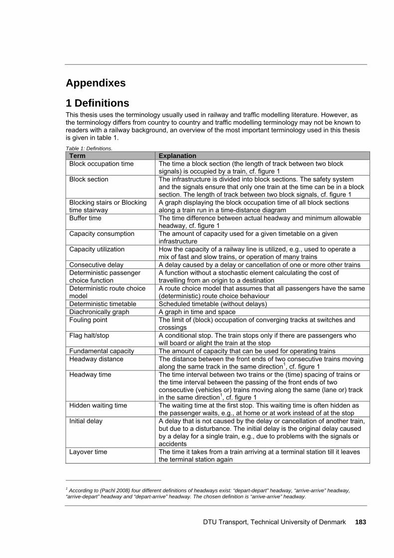
DTU Transport, Technical University of Denmark 183
Appendixes
1 Definitions This thesis uses the terminology usually used in railway and traffic modelling literature. However, as the terminology differs from country to country and traffic modelling terminology may not be known to readers with a railway background, an overview of the most important terminology used in this thesis is given in table 1. Table 1: Definitions. Term Explanation Block occupation time The time a block section (the length of track between two block
signals) is occupied by a train, cf. figure 1 Block section The infrastructure is divided into block sections. The safety system
and the signals ensure that only one train at the time can be in a block section. The length of track between two block signals, cf. figure 1
Blocking stairs or Blocking time stairway
A graph displaying the block occupation time of all block sections along a train run in a time-distance diagram
Buffer time The time difference between actual headway and minimum allowable headway, cf. figure 1
Capacity consumption The amount of capacity used for a given timetable on a given infrastructure
Capacity utilization How the capacity of a railway line is utilized, e.g., used to operate a mix of fast and slow trains, or operation of many trains
Consecutive delay A delay caused by a delay or cancellation of one or more other trains Deterministic passenger choice function
A function without a stochastic element calculating the cost of travelling from an origin to a destination
Deterministic route choice model
A route choice model that assumes that all passengers have the same (deterministic) route choice behaviour
Deterministic timetable Scheduled timetable (without delays) Diachronically graph A graph in time and space Fouling point The limit of (block) occupation of converging tracks at switches and
crossings Flag halt/stop A conditional stop. The train stops only if there are passengers who
will board or alight the train at the stop Fundamental capacity The amount of capacity that can be used for operating trains Headway distance The distance between the front ends of two consecutive trains moving
along the same track in the same direction1, cf. figure 1 Headway time The time interval between two trains or the (time) spacing of trains or
the time interval between the passing of the front ends of two consecutive (vehicles or) trains moving along the same (lane or) track in the same direction1, cf. figure 1
Hidden waiting time The waiting time at the first stop. This waiting time is often hidden as the passenger waits, e.g., at home or at work instead of at the stop
Initial delay A delay that is not caused by the delay or cancellation of another train, but due to a disturbance. The initial delay is the original delay caused by a delay for a single train, e.g., due to problems with the signals or accidents
Layover time The time it takes from a train arriving at a terminal station till it leaves the terminal station again
1 According to (Pachl 2008) four different definitions of headways exist: “depart-depart” headway, “arrive-arrive” headway, “arrive-depart” headway and “depart-arrive” headway. The chosen definition is “arrive-arrive” headway.
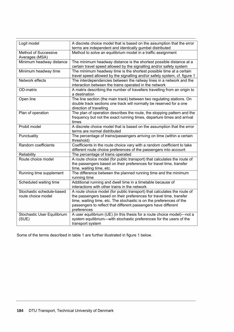
184 DTU Transport, Technical University of Denmark
Logit model A discrete choice model that is based on the assumption that the error terms are independent and identically gumbel distributed
Method of Successive Averages (MSA)
Method to solve an equilibrium model in a traffic assignment
Minimum headway distance The minimum headway distance is the shortest possible distance at a certain travel speed allowed by the signalling and/or safety system
Minimum headway time The minimum headway time is the shortest possible time at a certain travel speed allowed by the signalling and/or safety system, cf. figure 1
Network effects The interdependencies between the railway lines in a network and the interaction between the trains operated in the network
OD-matrix A matrix describing the number of travellers travelling from an origin to a destination
Open line The line section (the main track) between two regulating stations. On double track sections one track will normally be reserved for a one direction of travelling
Plan of operation The plan of operation describes the route, the stopping pattern and the frequency but not the exact running times, departure times and arrival times
Probit model A discrete choice model that is based on the assumption that the error terms are normal distributed
Punctuality The percentage of trains/passengers arriving on time (within a certain threshold)
Random coefficients Coefficients in the route choice vary with a random coefficient to take different route choice preferences of the passengers into account
Reliability The percentage of trains operated Route choice model A route choice model (for public transport) that calculates the route of
the passengers based on their preferences for travel time, transfer time, waiting time, etc.
Running time supplement The difference between the planned running time and the minimum running time
Scheduled waiting time Additional running and dwell time in a timetable because of interactions with other trains in the network
Stochastic schedule-based route choice model
A route choice model (for public transport) that calculates the route of the passengers based on their preferences for travel time, transfer time, waiting time, etc. The stochastic is on the preferences of the passengers to reflect that different passengers have different preferences
Stochastic User Equilibrium (SUE)
A user equilibrium (UE) (in this thesis for a route choice model)—not a system equilibrium—with stochastic preferences for the users of the transport system
Some of the terms described in table 1 are further illustrated in figure 1 below.

DTU Transport, Technical University of Denmark 185
Distance
Headway time
Buffer time
Minimum headway timeBlock section
Block occupation time
Time
Headway distance
Figure 1: Definitions. Based on (Landex, Kaas 2005).

186 DTU Transport, Technical University of Denmark

DTU Transport, Technical University of Denmark 187
2 Symbols Symbol Explanation a Number of line sections ar The braking rate fd The desired frequency fm,ij Occupation time for train route combinations hN Number of headways hN-1 Number of headways minus 1 hA
t,i Observed headway time at the end of line section i hA
t,i+1 Observed headway time at the end of line section i+1 hD
t,i Observed headway time at the beginning of line section i hD
t,i+1 Observed headway time at the beginning of line section i+1 h-
t,i Minimum headway time of a line section i Counter j Counter k The total capacity consumption K Capacity consumption in per cent LT Length of train LT,1 Length of train 1 LT,2 Length of train 2 LX Length of crossing track LX,1 Length of crossing track for train 1 LX,2 Length of crossing track for train 2 n Multiplication factor ni Number of trains using train route i nj Number of trains using train route j N Number of trains nk Number of train routes that cannot be set at the same time nt Number of tracks nΣ Total number of different combination possibilities of train routes that can be set after each
other NT Number of train types pk The sum of the possibilities of train routes that cannot be set at the same time pk,A The sum of the probabilities of train routes that cannot be set at the same time for station A pk,B The sum of the probabilities of train routes that cannot be set at the same time for station B pk,ij Probability of conflicts between train route i and j pΣ Sum of probabilities of train routes that can be set after each other Sb The braking distance SS The safety distance behind a signal SS,1 The safety distance for train 1 SS,2 The safety distance for train 2 SAHR Sum of Arrival Headway time Reciprocals SSHR Sum of Shortest Headway time Reciprocals T Time period tA Infrastructure occupation time tb Buffer time tB Buffer time in UIC 406 capacity analyses
b
_
t The average buffer time tb,i,c The buffer time between the initial train and the succeeding train tC Time supplement for single track lines td,1,i The initial delay of train 1 td,2,c The consecutive delay of train 2 td,j+1,c The consecutive delay of train j+1 td,x,c The consecutive delay of train x tD Time supplement for maintenance

188 DTU Transport, Technical University of Denmark
th Headway time h
_t Average headway time th,d The desired headway time th,min The minimum headway time th,min,ij Minimum headway time of train route i followed by train route j th,min,cc Minimum headway time of train route c followed by train route c th,min,dd Minimum headway time of train route d followed by train route d to Total time the train routes are occupied to,A Total time the train routes are occupied at station A to,B Total time the train routes are occupied at station B tR The reaction time of the engine driver and the braking system of the train tU The time window examined tx The running time between two crossovers tx,AB The running time between two crossovers in the direction from A to B tx,BA The running time between two crossovers in the direction from B to A v The speed V The deviation from the optimal speed vi Speed of train i vopt The optimal speed (resulting in minimum capacity consumption) vt The speed of train type t vt,opt The optimal speed of train type t vx,max The maximum speed for a crossing whilst in motion W The complexity of a station based on the headway times WA The complexity of station A based on the headway times WB The complexity of station B based on the headway times WKh The complexity of Copenhagen central station based on the headway times WKk The complexity of Østerport station based on the headway times WSlb The complexity of Skelbæk technical station based on the headway times WUnd The complexity of Hundige station based on the headway times yt,d,1,i Delay propagation factor for the initial delay of train 1 qmax Maximum traffic intensity |Δth| The numeric difference in headway time from the beginning to the end of the line section ϕn Complexity of a station based on the track layout ϕn,A Complexity of station A based on the track layout ϕn,B Complexity of station B based on the track layout ϕn,Kh Complexity of Copenhagen central station based on the track layout ϕn,Kk Complexity of Østerport station based on the track layout ϕn,Slb Complexity of Skelbæk technical station based on the track layout ϕn,Und Complexity of Hundige station based on the track layout ϕp Complexity of a station based on probabilities of train routes set after each other ϕp,A Complexity of a station based on probabilities of train routes set after each other for station
A ϕp,B Complexity of a station based on probabilities of train routes set after each other for station
B ϕp,Kh Complexity of a station based on probabilities of train routes set after each other for
Copenhagen central station ϕp,Kk Complexity of a station based on probabilities of train routes set after each other for
Østerport station ϕp,Slb Complexity of a station based on probabilities of train routes set after each other for
Skelbæk technical station ϕp,Und Complexity of a station based on probabilities of train routes set after each other for
Hundige station Σtd The total amount of (train) delay
d
~tΣ Total amount of estimated (train) delay
Σtd,TS,a Sum of delay for all train sequences of a single track line Σtd,x,c The total amount of consecutive delays
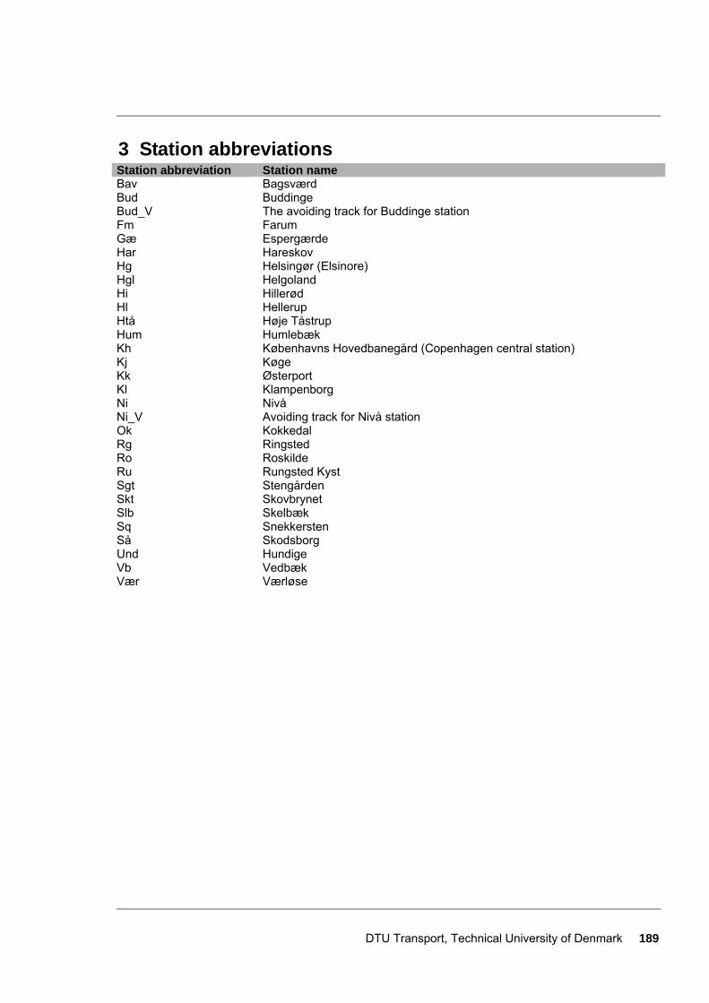
DTU Transport, Technical University of Denmark 189
3 Station abbreviations Station abbreviation Station name Bav Bagsværd Bud Buddinge Bud_V The avoiding track for Buddinge station Fm Farum Gæ Espergærde Har Hareskov Hg Helsingør (Elsinore) Hgl Helgoland Hi Hillerød Hl Hellerup Htå Høje Tåstrup Hum Humlebæk Kh Københavns Hovedbanegård (Copenhagen central station) Kj Køge Kk Østerport Kl Klampenborg Ni Nivå Ni_V Avoiding track for Nivå station Ok Kokkedal Rg Ringsted Ro Roskilde Ru Rungsted Kyst Sgt Stengården Skt Skovbrynet Slb Skelbæk Sq Snekkersten Så Skodsborg Und Hundige Vb Vedbæk Vær Værløse

190 DTU Transport, Technical University of Denmark
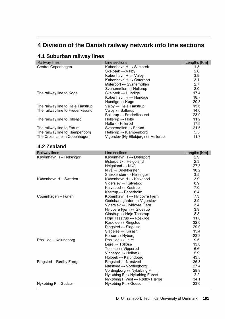
DTU Transport, Technical University of Denmark 191
4 Division of the Danish railway network into line sections
4.1 Suburban railway lines Railway lines Line sections Lengths [Km] Central Copenhagen København H → Skelbæk 1.3
Skelbæk → Valby 2.6 København H ← Valby 3.9 København H ↔ Østerport 3.1 Østerport ↔ Svanemøllen 2,7 Svanemøllen ↔ Hellerup 2.0
The railway line to Køge Skelbæk → Hundige 17.4 København H ← Hundige 18.7 Hundige ↔ Køge 20.3
The railway line to Høje Taastrup Valby ↔ Høje Taastrup 15.6 The railway line to Frederikssund Valby ↔ Ballerup 14.0
Ballerup ↔ Frederikssund 23.9 The railway line to Hillerød Hellerup ↔ Holte 11.2
Holte ↔ Hillerød 17.5 The railway line to Farum Svanemøllen ↔ Farum 21.5 The railway line to Klampenborg Hellerup ↔ Klampenborg 5.5 The Cross Line in Copenhagen Vigerslev (Ny Ellebjerg) ↔ Hellerup 11.7
4.2 Zealand Railway lines Line sections Lengths [Km] København H – Helsingør København H ↔ Østerport 2.9
Østerport ↔ Helgoland 2.3 Helgoland ↔ Nivå 27.3 Nivå ↔ Snekkersten 10.2 Snekkersten ↔ Helsingør 3.5
København H – Sweden København H ↔ Kalvebod 3.9 Vigerslev ↔ Kalvebod 0.9 Kalvebod ↔ Kastrup 7.0 Kastrup ↔ Peberholm 6.4
Copenhagen – Funen København H ↔ Hvidovre Fjern 7.3 Godsbanegården ↔ Vigerslev 3.9 Vigerslev ↔ Hvidovre Fjern 3.4 Hvidovre Fjern ↔ Glostrup 3.9 Glostrup ↔ Høje Taastrup 8.3 Høje Taastrup ↔ Roskilde 11.8 Roskilde ↔ Ringsted 32.6 Ringsted ↔ Slagelse 29.0 Slagelse ↔ Korsør 15.4 Korsør ↔ Nyborg 23.3
Roskilde – Kalundborg Roskilde ↔ Lejre 9.5 Lejre ↔ Tølløse 13.8 Tølløse ↔ Vipperød 6.6 Vipperød ↔ Holbæk 5.9 Holbæk ↔ Kalundborg 43.5
Ringsted – Rødby Færge Ringsted ↔ Næstved 26.8 Næstved ↔ Vordingborg 27.4 Vordingborg ↔ Nykøbing F 28.8 Nykøbing F ↔ Nykøbing F Vest 2.2 Nykøbing F Vest ↔ Rødby Færge 34.1
Nykøbing F – Gedser Nykøbing F ↔ Gedser 23.0
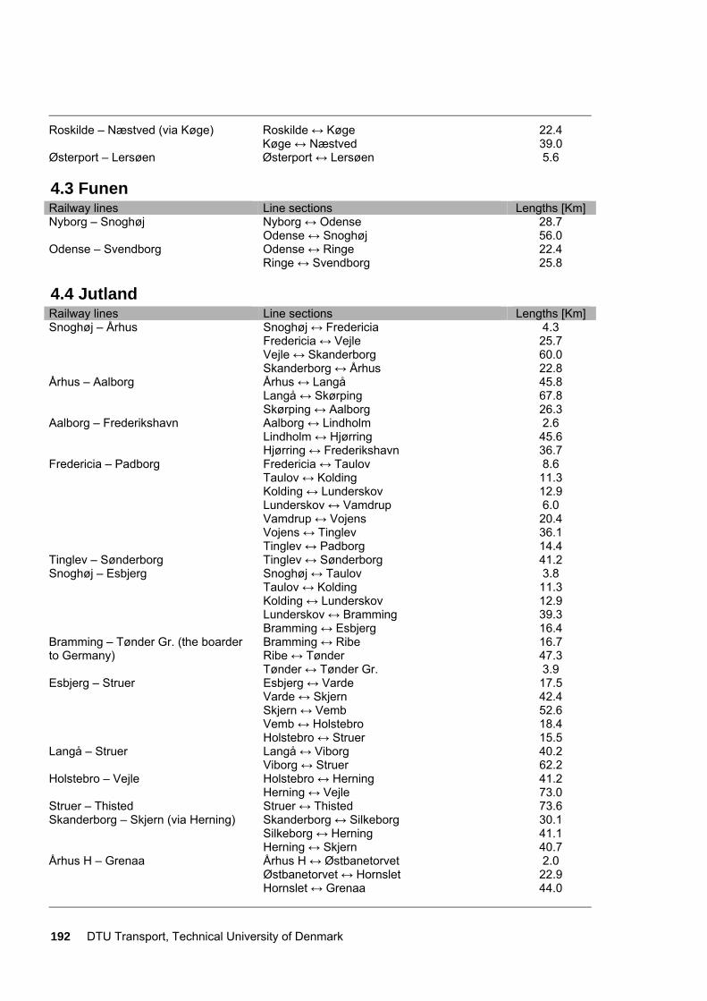
192 DTU Transport, Technical University of Denmark
Roskilde – Næstved (via Køge) Roskilde ↔ Køge 22.4 Køge ↔ Næstved 39.0
Østerport – Lersøen Østerport ↔ Lersøen 5.6
4.3 Funen Railway lines Line sections Lengths [Km] Nyborg – Snoghøj Nyborg ↔ Odense 28.7
Odense ↔ Snoghøj 56.0 Odense – Svendborg Odense ↔ Ringe 22.4
Ringe ↔ Svendborg 25.8
4.4 Jutland Railway lines Line sections Lengths [Km] Snoghøj – Århus Snoghøj ↔ Fredericia 4.3
Fredericia ↔ Vejle 25.7 Vejle ↔ Skanderborg 60.0 Skanderborg ↔ Århus 22.8
Århus – Aalborg Århus ↔ Langå 45.8 Langå ↔ Skørping 67.8 Skørping ↔ Aalborg 26.3
Aalborg – Frederikshavn Aalborg ↔ Lindholm 2.6 Lindholm ↔ Hjørring 45.6 Hjørring ↔ Frederikshavn 36.7
Fredericia – Padborg Fredericia ↔ Taulov 8.6 Taulov ↔ Kolding 11.3 Kolding ↔ Lunderskov 12.9 Lunderskov ↔ Vamdrup 6.0 Vamdrup ↔ Vojens 20.4 Vojens ↔ Tinglev 36.1 Tinglev ↔ Padborg 14.4
Tinglev – Sønderborg Tinglev ↔ Sønderborg 41.2 Snoghøj – Esbjerg Snoghøj ↔ Taulov 3.8
Taulov ↔ Kolding 11.3 Kolding ↔ Lunderskov 12.9 Lunderskov ↔ Bramming 39.3 Bramming ↔ Esbjerg 16.4
Bramming – Tønder Gr. (the boarder to Germany)
Bramming ↔ Ribe 16.7 Ribe ↔ Tønder 47.3 Tønder ↔ Tønder Gr. 3.9
Esbjerg – Struer Esbjerg ↔ Varde 17.5 Varde ↔ Skjern 42.4 Skjern ↔ Vemb 52.6 Vemb ↔ Holstebro 18.4 Holstebro ↔ Struer 15.5
Langå – Struer Langå ↔ Viborg 40.2 Viborg ↔ Struer 62.2
Holstebro – Vejle Holstebro ↔ Herning 41.2 Herning ↔ Vejle 73.0
Struer – Thisted Struer ↔ Thisted 73.6 Skanderborg – Skjern (via Herning) Skanderborg ↔ Silkeborg 30.1
Silkeborg ↔ Herning 41.1 Herning ↔ Skjern 40.7
Århus H – Grenaa Århus H ↔ Østbanetorvet 2.0 Østbanetorvet ↔ Hornslet 22.9 Hornslet ↔ Grenaa 44.0
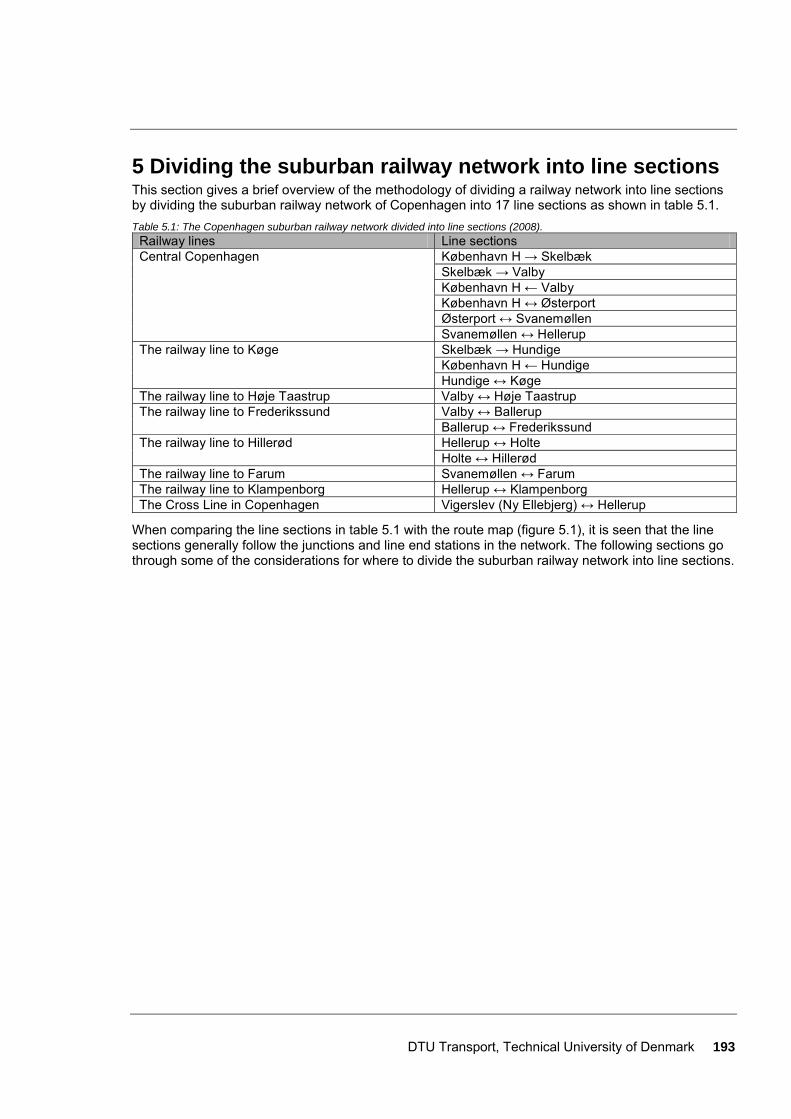
DTU Transport, Technical University of Denmark 193
5 Dividing the suburban railway network into line sections This section gives a brief overview of the methodology of dividing a railway network into line sections by dividing the suburban railway network of Copenhagen into 17 line sections as shown in table 5.1. Table 5.1: The Copenhagen suburban railway network divided into line sections (2008).
Railway lines Line sections København H → Skelbæk Skelbæk → Valby København H ← Valby København H ↔ Østerport Østerport ↔ Svanemøllen
Central Copenhagen
Svanemøllen ↔ Hellerup Skelbæk → Hundige København H ← Hundige
The railway line to Køge
Hundige ↔ Køge The railway line to Høje Taastrup Valby ↔ Høje Taastrup
Valby ↔ Ballerup The railway line to Frederikssund Ballerup ↔ Frederikssund Hellerup ↔ Holte The railway line to Hillerød Holte ↔ Hillerød
The railway line to Farum Svanemøllen ↔ Farum The railway line to Klampenborg Hellerup ↔ Klampenborg The Cross Line in Copenhagen Vigerslev (Ny Ellebjerg) ↔ Hellerup
When comparing the line sections in table 5.1 with the route map (figure 5.1), it is seen that the line sections generally follow the junctions and line end stations in the network. The following sections go through some of the considerations for where to divide the suburban railway network into line sections.
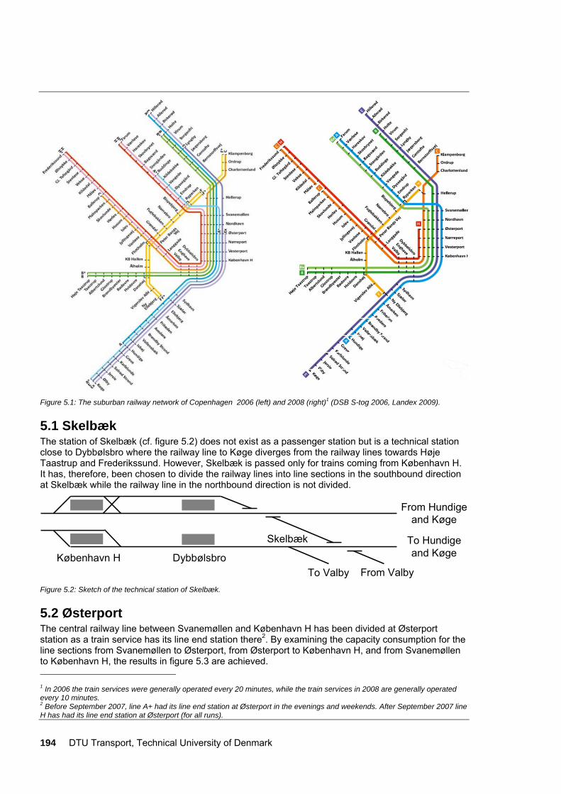
194 DTU Transport, Technical University of Denmark
Figure 5.1: The suburban railway network of Copenhagen 2006 (left) and 2008 (right)1 (DSB S-tog 2006, Landex 2009).
5.1 Skelbæk The station of Skelbæk (cf. figure 5.2) does not exist as a passenger station but is a technical station close to Dybbølsbro where the railway line to Køge diverges from the railway lines towards Høje Taastrup and Frederikssund. However, Skelbæk is passed only for trains coming from København H. It has, therefore, been chosen to divide the railway lines into line sections in the southbound direction at Skelbæk while the railway line in the northbound direction is not divided.
From Valby
To Hundigeand Køge
From Hundigeand Køge
To ValbyDybbølsbroKøbenhavn H
Skelbæk
Figure 5.2: Sketch of the technical station of Skelbæk.
5.2 Østerport The central railway line between Svanemøllen and København H has been divided at Østerport station as a train service has its line end station there2. By examining the capacity consumption for the line sections from Svanemøllen to Østerport, from Østerport to København H, and from Svanemøllen to København H, the results in figure 5.3 are achieved. 1 In 2006 the train services were generally operated every 20 minutes, while the train services in 2008 are generally operated every 10 minutes. 2 Before September 2007, line A+ had its line end station at Østerport in the evenings and weekends. After September 2007 line H has had its line end station at Østerport (for all runs).
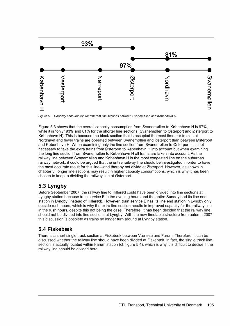
DTU Transport, Technical University of Denmark 195
Østerport
Nørreport
Svanem
øllen
Nordhavn
Vesterport
København H
93%
81%
97%
93%93%
81%81%
97%97%
Figure 5.3: Capacity consumption for different line sections between Svanemøllen and København H.
Figure 5.3 shows that the overall capacity consumption from Svanemøllen to København H is 97%, while it is “only” 93% and 81% for the shorter line sections (Svanemøllen to Østerport and Østerport to København H). This is because the block section that is occupied the most time per train is at Nordhavn and fewer trains are operated between Svanemøllen and Østerport than between Østerport and København H. When examining only the line section from Svanemøllen to Østerport, it is not necessary to take the extra trains from Østerport to København H into account but when examining the long line section from Svanemøllen to København H all trains are taken into account. As the railway line between Svanemøllen and København H is the most congested line on the suburban railway network, it could be argued that the entire railway line should be investigated in order to have the most accurate result for this line—and thereby not divide at Østerport. However, as shown in chapter 3, longer line sections may result in higher capacity consumptions, which is why it has been chosen to keep to dividing the railway line at Østerport.
5.3 Lyngby Before September 2007, the railway line to Hillerød could have been divided into line sections at Lyngby station because train service E in the evening hours and the entire Sunday had its line end station in Lyngby (instead of Hillerød). However, train service E has its line end station in Lyngby only outside rush hours, which is why the extra line section results in improved capacity for the railway line in the rush hours, despite this not being the case. Therefore, it has been decided that the railway line should not be divided into line sections at Lyngby. With the new timetable structure from autumn 2007 this discussion is obsolete as trains no longer turn around at Lyngby station.
5.4 Fiskebæk There is a short single track section at Fiskebæk between Værløse and Farum. Therefore, it can be discussed whether the railway line should have been divided at Fiskebæk. In fact, the single track line section is actually located within Farum station (cf. figure 5.4), which is why it is difficult to decide if the railway line should be divided here.
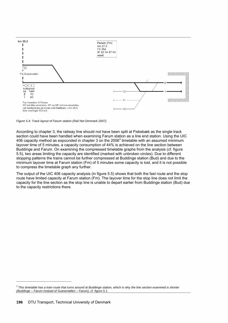
196 DTU Transport, Technical University of Denmark
Figure 5.4: Track layout of Farum station (Rail Net Denmark 2007).
According to chapter 3, the railway line should not have been split at Fiskebæk as the single track section could have been handled when examining Farum station as a line end station. Using the UIC 406 capacity method as expounded in chapter 3 on the 20063 timetable with an assumed minimum layover time of 5 minutes, a capacity consumption of 44% is achieved on the line section between Buddinge and Farum. On examining the compressed timetable graphs from the analysis (cf. figure 5.5), two areas limiting the capacity are identified (marked with unbroken circles). Due to different stopping patterns the trains cannot be further compressed at Buddinge station (Bud) and due to the minimum layover time at Farum station (Fm) of 5 minutes some capacity is lost, and it is not possible to compress the timetable graph any further.
The output of the UIC 406 capacity analysis (in figure 5.5) shows that both the fast route and the stop route have limited capacity at Farum station (Fm). The layover time for the stop line does not limit the capacity for the line section as the stop line is unable to depart earlier from Buddinge station (Bud) due to the capacity restrictions there.
3 This timetable has a train route that turns around at Buddinge station, which is why the line section examined is shorter (Buddinge – Farum instead of Svanemøllen – Farum), cf. figure 5.1.
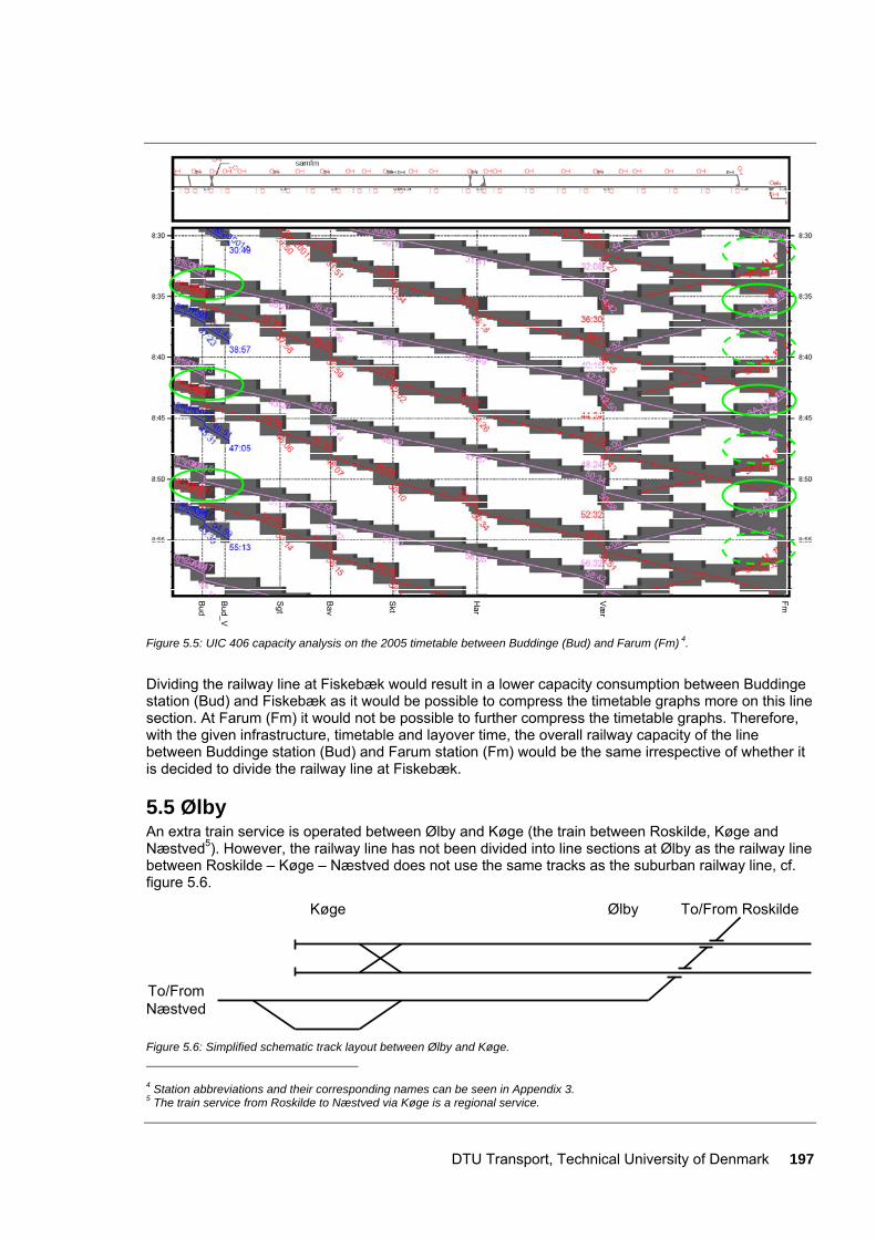
DTU Transport, Technical University of Denmark 197
Bud
Vær
FmBud_V
Sgt
Bav
Skt
Har
Figure 5.5: UIC 406 capacity analysis on the 2005 timetable between Buddinge (Bud) and Farum (Fm) 4.
Dividing the railway line at Fiskebæk would result in a lower capacity consumption between Buddinge station (Bud) and Fiskebæk as it would be possible to compress the timetable graphs more on this line section. At Farum (Fm) it would not be possible to further compress the timetable graphs. Therefore, with the given infrastructure, timetable and layover time, the overall railway capacity of the line between Buddinge station (Bud) and Farum station (Fm) would be the same irrespective of whether it is decided to divide the railway line at Fiskebæk.
5.5 Ølby An extra train service is operated between Ølby and Køge (the train between Roskilde, Køge and Næstved5). However, the railway line has not been divided into line sections at Ølby as the railway line between Roskilde – Køge – Næstved does not use the same tracks as the suburban railway line, cf. figure 5.6.
To/From RoskildeKøge
To/FromNæstved
Ølby
Figure 5.6: Simplified schematic track layout between Ølby and Køge. 4 Station abbreviations and their corresponding names can be seen in Appendix 3. 5 The train service from Roskilde to Næstved via Køge is a regional service.

198 DTU Transport, Technical University of Denmark
5.6 The Cross Line Looking at the suburban Cross Line two aspects are apparent: Vigerslev station does not exist on the route map (only Vigerslev Alle exists) and the cross line is not divided into line sections when crossing other railway lines. Vigerslev is a technical station covering the line end station of Ny Ellebjerg, which is why the two names express the same location. The cross line is not divided into line sections when crossing other railway lines as the crossings are out of grade (and without the possibility to change between the lines) except at Hellerup station.
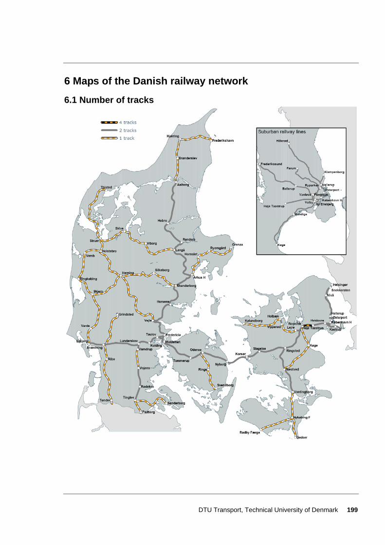
DTU Transport, Technical University of Denmark 199
6 Maps of the Danish railway network
6.1 Number of tracks
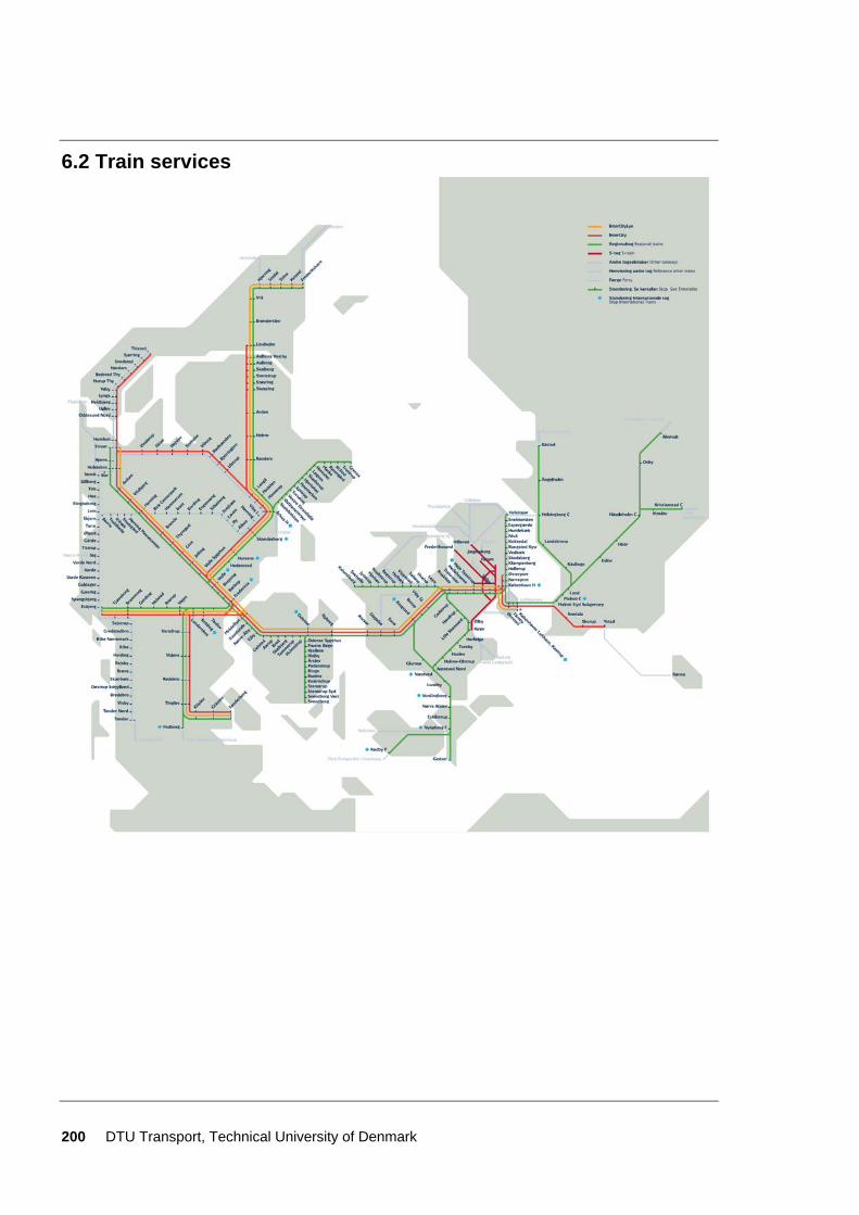
200 DTU Transport, Technical University of Denmark
6.2 Train services
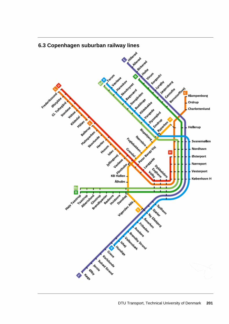
DTU Transport, Technical University of Denmark 201
6.3 Copenhagen suburban railway lines
