methods of analysis - robert l. bertinibertini.eng.usf.edu/courses/559/methods_of_analysis.pdf ·...

Methods of Analysis for Transportation Operations

by

Carlos F. Daganzo and

Gordon F. Newell

Revised 2/07


ii

OUTLINE

1. Introduction..........................................................................................................................1

2. Queueing Theory .................................................................................................................4

2.1 Graphical representation ..........................................................................................5

2.2 Approximations......................................................................................................12

2.3 Stochastic Properties of Queues.............................................................................15

2.4 Equilibrium Queues ...............................................................................................20

2.5 Examples................................................................................................................23

2.6 Queueing of Two Conflicting Traffic Streams ......................................................29

3. Time-Space Diagrams........................................................................................................37

3.1 Analysis of Vehicular Movement (One Vehicle) ..................................................37

3.2 Analysis of Vehicular Movement (Several Vehicles) ...........................................42

3.3 The Fundamental Relationship of Flow and the Fundamental Diagram ...............44

3.4 Examples................................................................................................................56

4. Modelling Energy, Air Pollution, and Noise .....................................................................64

4.1 Modelling Philosophy............................................................................................65

4.2 Energy Consumption .............................................................................................65

4.3 Air Pollution...........................................................................................................67

4.4 Noise ......................................................................................................................70

5. References..........................................................................................................................73

Daganzo and Newell

iii

Daganzo and Newell

1

1. INTRODUCTION

The attractiveness of a transportation facility to its users is determined by factors such as

safety, speed of service, and comfort. Sometimes it is possible to represent the combined effect

of all these factors into one general measure of performance which we will call level of service.

A facility which provides a high level of service is a facility which is quick, cheap and

comfortable to use and which is perceived as safe by its users. When the level of service can be

translated into monetary units, one defines instead a generalized price (or generalized cost)

which can be used for economic evaluation purposes and feasibility analyses.

Most of the emphasis of these notes is on predicting the time that it takes for a given user

(person or good) to use a transportation facility since travel time is one of the main components

of generalized cost. Although it is not possible to determine exactly how much people value

travel time (it has been said to be around one-third of the hourly wage), it is important to have a

rough idea so that one can relate travel time to generalized price. The value of time to shippers of

material goods can be assessed more easily. It is related to their inventory costs because with

slow transportation systems shippers must re-order when their stock levels are still high in order

to avoid stockouts. The value of time varies enormously from commodity to commodity.

However, as happens with humans, it turns out that high value items have higher values of time.


2

The ability to both transform travel time into monetary units (generalized cost) and

predict travel time allows one to perform cost-effectiveness analyses in the design of

transportation facilities by trading off travel time versus construction and operation cost. This

handout provides two important analysis tools for predicting travel time in transportation

facilities: Queueing theory and the time-space diagram.

All transportation facilities are subject to rush hours, seasonal variations, and long-time

trends in demand. It is not generally economical to provide facilities so as to accommodate the

peak demand, because that last increment of capacity which one would provide to serve the peak

would be used for essentially zero time. In such case, one would obtain virtually zero benefit per

unit of investment. Queueing theory helps analysts in situations like these by enabling them to

estimate user delays at transportation facilities when, occasionally, demand exceeds capacity.

The time-space diagram is a tool that is used to study the way in which vehicles overcome

distance. Each of these two tools has its specific applications area. For instance, if one realizes

that in most transportation systems vehicles are confined to channels and that along these

channels there are bottlenecks (i.e., points where flow is restricted), one can visualize queueing

theory as the study of bottlenecks and time-space theory as the study of vehicular movement

between bottlenecks. Some transportation studies require the use of both theories; for instance,

analyzing shipping along a waterway requires queueing theory to study the waiting lines at the

Daganzo and Newell

3

entrance of the waterway and time-space diagrams to generate ship schedules that will ensure

that ships cross safely at predetermined sidings.

Transportation engineers, however, are not only concerned with delays to the users of a

transportation facility; they must also understand the other elements of level of service and the

impact that a facility has on non-users. Some of these impacts (such as aesthetics) cannot be

quantified, and some (such as comfort) do not depend much on the way the transportation facility

is being used. Since one does not need much technical knowledge to evaluate these, they are not

explored in this handout. Some impacts, however, are heavily dependent on the way the facility

is being used, e.g., safety, noise, energy consumption, and air pollution, and (except for safety

which requires sophisticated statistical analyses) can be studied with queueing and time-space

studies. This is done in the last part of these notes.


4

2. QUEUEING THEORY

Queueing theory studies congestion phenomena, i.e., the behavior of objects passing

through a point at which there is a restriction on the maximum rate at which they can get through.

A queueing system can be represented schematically as follows:

Figure 1

Most queueing systems have a storage area upstream of the restriction where the objects that

have arrived but have not yet passed through the restriction are queued up. The collection of

objects in the storage area is called a queue. Because queueing theory was developed with a

certain type of application in mind (such as the analysis of waiting lines at check-out counters)

the objects are referred to as customers and the restriction as a server (or service station if it

contains more than one server).

Examples of transportation queueing problems are aircraft requiring to take-off,

automobiles arriving at a toll gate, passengers waiting for elevators, and ships calling at a port. In

all these examples the customers are transportation vehicles (except in the elevator case where

Daganzo and Newell

5

the passengers are the objects) and the restrictions to flow are respectively the runway, the toll

gate, the elevator doors, and the entrance to the port.

With queueing theory one can study the behavior of a queue over time if the input stream

(or arrival process) of customers and the characteristics of the restriction (or service

mechanism) are known. One is usually interested in the maximum queue length over a period of

time and on typical waiting (or queueing) times. This is explained in the rest of this chapter.

2.1 Graphical Representation

Queueing problems arise in other areas of civil engineering. The analysis of water storage

over time in a reservoir is a queueing problem in which the water runoff into the reservoir is the

customer, the dam is the server, and the reservoir itself is the storage area. Queueing techniques

are commonly used to size reservoirs.

The basic principle underlying queueing theory (similar to the conservation principle of

mechanics of fluids, hydraulics and physics) is that customers do not disappear; i.e., the increase

in the number of customers in the storage area during time ∆t equals the number of customers

that have arrived in ∆t minus the number to have departed. This feature is exploited later on to

derive the properties of a queueing system.

Suppose, starting with an empty system, objects arrive at the storage at discrete times,


6

0 ≤ t1 ≤ t2 ≤ …

and that these times are known.

This information completely characterizes the arrival process (i.e., it is all we need to

know) for queueing theory purposes. It is conveniently summarized in a graph of the cumulative

number of customers to have arrived by time t, j, vs. time.

Figure 2

Note that A(t) is a function that increases by 1 at each tj and equals zero at the time we

start counting customers.

The inverse function t = A-1(j) can be visualized as the time at which the jth object arrives.

Of course, if j is not integer this interpretation is not meaningful unless we visualize j = 2.5 as

Daganzo and Newell

7

representing the first two objects and one-half of the third one. In such case, and since objects are

indivisible A-1(2.5) = t3 (see Figure 2).

If we know the service mechanism, i.e., how fast customers are processed through the

system it is possible to determine the times at which customers leave the system and to draw a

curve depicting the cumulative number of customers to have departed by time t, D(t). The way in

which the departure curve, D(t) is obtained from the arrival curve and the service mechanism is

explored later. For our present purposes we simply suppose that the D(t) curve has been recorded

by an observer and proceed to show how one can determine queue lengths and waiting times

from the A(t) and D(t) curves when they are plotted on the same graph. This is done in Figure 3.

In this figure the departure times are distinguished from the arrival times by primes.

Figure 3


8

If, as in the above figure, the system is empty at time t = 0 and we start the A(t) and D(t)

counts at t = 0, the vertical distance between A(t) and D(t) gives the queue length (the number of

people in storage) at time t, Q(t), since by the conservation principle

Q(t) – Q(0) = [A(t) – A(0)] – [D(t) – D(0)].

and in our case Q(0) = A(0) = D(0) = 0. Thus,

Q(t) = A(t) – D(t).

Note that A(t) and D(t) can never cross because the number of people in storage cannot be

negative. If at time t = 0 there is an initial queue Q(0) the formula is instead Q(t) = Q(0) + A(t) –

D(t) and the vertical distances no longer represent queue lengths. This can be corrected by

shifting the A(t) curve upwards Q(0) units, as in that case A(0) = Q(0) and the conservation

equation also yields:

Q(t) = A(t) – D(t).

In the remainder of this handout we assume that the arrival and departure curves are drawn so

that Q(t) = A(t) – D(t).

Horizontal distances also have a simple interpretation. If we consecutively number the

customers with labels j = 1, 2, 3,… in the order of arrival, and if customers are served in the

same order in which they arrive (First-In-First-Out), the jth cumulative departure is also the

object with label j. It leaves at the time of the jth jump of the departure curve:

Daganzo and Newell

9

t′j = D-1(j).

Thus for FIFO, the waiting time to the jth customer, wj, (the difference between its

departure and arrival times, t′j – tj) is given by the horizontal distance between A(t) and D(t):

wj = D-1(j) – A-1(j).

As some global measure of performance, it is often convenient to evaluate the total time

spent by objects in the storage. One may be interested in either the total time spent in the system

by a specified number of objects, or in the total time spent by all objects during a specific period

of observation.

In the former case, for FIFO, we can interpret the wj either as the horizontal distance

between A(t) and D(t) or as the area of a horizontal strip of unit height and width wj (see Figure

4). The total delay to objects 1, 2, …., n is the sum of the areas of strips 1 to n, i.e., the total area

between A(t) and D(t) and lines at height 0 an n.


10

Figure 4

The average waiting time to the n customers is, thus

nw

nw

n

ij

Area11

=×= ∑=

If customers are not served according to a first-in-first-out rule, it is difficult to obtain

their individual waiting times from the A(t) and D(t) plot and the above arguments (the

expressions for wj and w ) are not valid.

In the latter case we can say that the total time spent in the system by customers during a

time period t to t + dt is Q(t)dt (see Figure 5). Note that this is a fact entirely independent of the

order in which customers are served. The total time spent in storage by all customers during time

0 to T is:

Daganzo and Newell

11

∫ ∫ −==T T

dttDtAdttQTT0 0

)]()([)(

This has the geometrical interpretation of the area between A(t) and D(t), and the two vertical

lines at 0 and T.

Figure 5

If storage is empty at time T, when the nth object leaves, the two areas are the same.

Figure 6


12

∫ =≡=T

dttQT

Q0 T

area)(1 storagein number average time (1)

∑ ===n

wn

w jarea1 storagein spendsobject timeaverage (2)

Eliminating the area from (1) and (2) we obtain an important relationship between w and Q :

;

area

wTn

Q

QTwn

=

==

where Tn is interpreted as the average number of arrivals per unit time. Thus, for any service

order and between points where the storage is empty we have:

Average queue length = Average waiting time × Average arrival rate.

2.2 Approximations

If one is concerned with systems for which Q(t) is typically 10 or 100 or more, and A(t)

will reach values of 100 or 1000 or more during the period of observation (as, for example, with

cars queueing behind a toll gate), one would draw graphs of A(t) and D(t) on such a scale that the

individual integer steps could hardly be seen. One may not even bother to measure the detailed

arrival times but only observe the counts A(t) at selected times (every five minutes, for example).

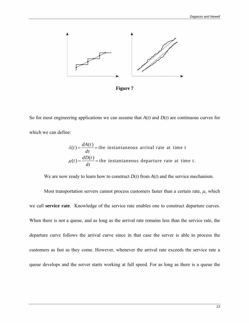
If one does observe the individual steps, one could approximate A(t) by a smoother curve drawn

through the midpoints of the vertical and horizontal steps.

Daganzo and Newell

13

Figure 7

So for most engineering applications we can assume that A(t) and D(t) are continuous curves for

which we can define:

. timeat rate departure ousinstantane the )(

)(

timeat rate arrival ousinstantane the )(

)(

tdt

tdDt

tdt

tdAt

==

==

µ

λ

We are now ready to learn how to construct D(t) from A(t) and the service mechanism.

Most transportation servers cannot process customers faster than a certain rate, µ, which

we call service rate. Knowledge of the service rate enables one to construct departure curves.

When there is not a queue, and as long as the arrival rate remains less than the service rate, the

departure curve follows the arrival curve since in that case the server is able to process the

customers as fast as they come. However, whenever the arrival rate exceeds the service rate a

queue develops and the server starts working at full speed. For as long as there is a queue the


14

departure curve is a straight line with slope, µ. When such a straight line meets the arrival curve,

the queue dissipates and the departure curve follows the arrival curve.

A typical situation is depicted in Figure 8:

Figure 8

Summarizing, there are three things that must be remembered when drawing D(t):

1. The departure rate cannot exceed the service rate of the server. It may be less.

2. Cumulative departures can never exceed cumulative arrivals. D(t) can never be

above A(t) on the queueing diagram.

3. When a queue is present, the departure rate will equal the service rate.

Of course, there are more complicated situations such as storage areas with limited

capacity, servers which turn themselves off and on periodically and servers whose service rate

Daganzo and Newell

15

changes with the queue length. Some of these will be studied later but the three items above

always apply.

2.3 Stochastic Properties of Queues

Generally one finds in analyzing queues for transportation systems, that the detailed

behavior of a system is not reproducible. If one repeats the observation another day under what

seems to be equivalent conditions, the new curves A(t), D(t) may, on a coarse scale, be nearly the

same as the old curves, but the exact times of the steps will be different, and the curves will, in

general have wiggles in different places.

If the typical queue lengths that develop every day are negligible in such coarse scale of

measurement, the value of Q(t) is determined by the wiggles more than by the general shape of

the curve and, consequently, may drastically vary from day to day. In such case, one would be

interested in the average behavior of the queue over a number of days (i.e., in the average arrival

curve, departure curve, queue length, and waiting time, and on the relationships among these).

The average arrival curve over n days is defined as:

∑=

=n

jj tA

ntA

1),(1)(


16

where Aj(t) is the arrival curve on the jth day. As n becomes larger, the wiggles on the arrival

curve on individual days tend to cancel with one another so that in most cases )(tA is a smooth

curve. The derivative of )(tA with respect to time

dttAdt )()( =λ

is called the average arrival rate.

The same thing could be done with the departure curves Dj(t), queue lengths Qj(t) and TT,

to obtain some average values )(tD , )(tQ , and TT .

It is not difficult to show from the definitions of )(tA , )(tD , )(tQ , and TT that

TT = area between )(tA and )(tD from 0 to T,

and that,

)(tQ = )(tA - )(tD .

Thus, if one could construct )(tD from )(tA one would determine )(tQ and TT .

Unfortunately, as is shown with the simple example below )(tD does not follow the same rules

as D(t) and one cannot in general determine it from A(t). Information regarding the arrival curves

for every day is needed.

Daganzo and Newell

17

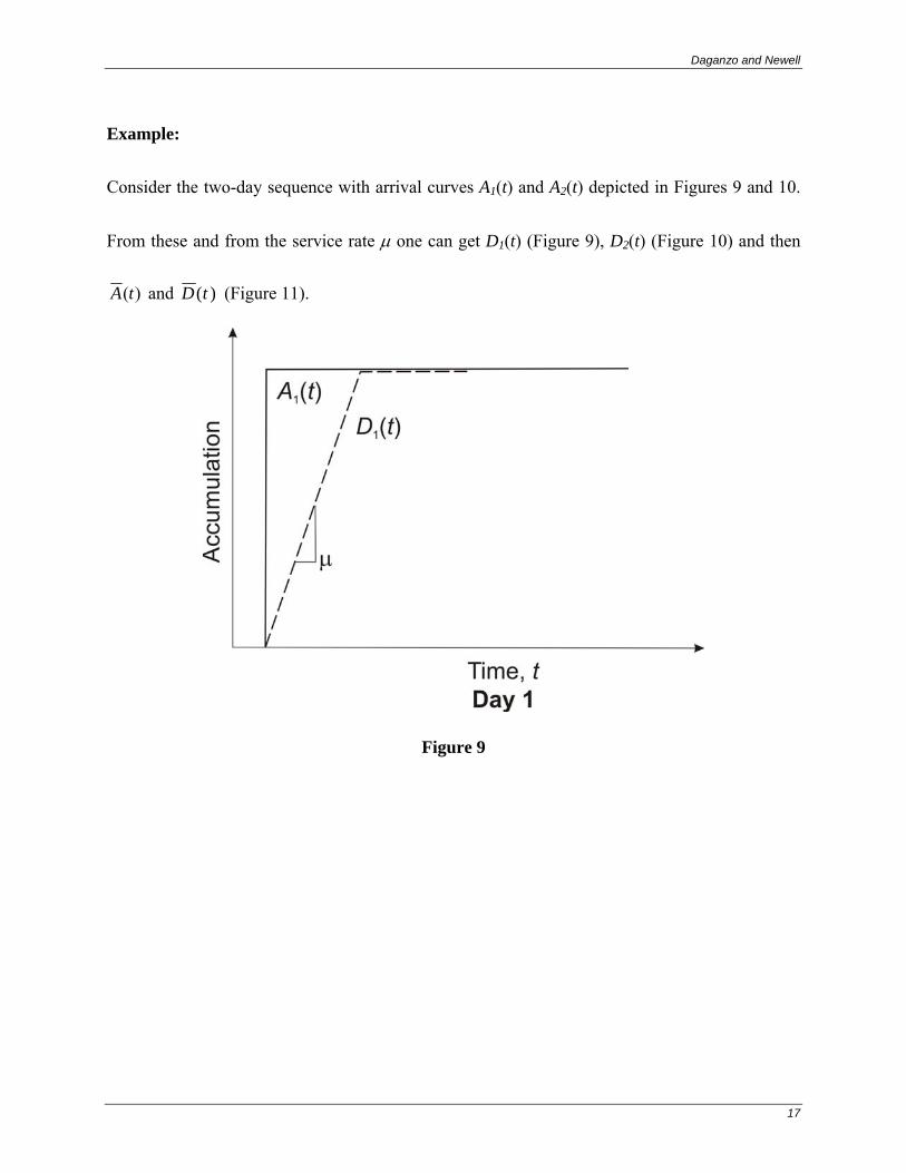
Example:

Consider the two-day sequence with arrival curves A1(t) and A2(t) depicted in Figures 9 and 10.

From these and from the service rate µ one can get D1(t) (Figure 9), D2(t) (Figure 10) and then

)(tA and )(tD (Figure 11).

Figure 9


18

Figure 10

Figure 11

Daganzo and Newell

19

However, if the arrival curves on days one and two had been the same, A1(t) = A2(t) =

)(tA , the average departure curve would have been different.

Figure 12

Thus, situations giving rise to the same average arrival curve will, in general, generate

different average departure curves and different queue lengths.

Note, also, that the average total delay, TT , is larger in the former case when the two

arrival curves were different. This is true, in general, since it can be mathematically proven that

both TT and )(tQ are larger when the arrival curves vary substantially from day to day.


20

It is thus difficult to estimate delays and queue lengths when only )(tA is known since

one needs some additional information in order to obtain )(tD . There are two instances,

however, when obtaining average queue lengths is extremely easy:

1. If the queue lengths that develop on a typical day are large compared with the wiggles

on Aj(t) from day to day, one can neglect the wiggles and approximately obtain )(tD

from )(tA or from the arrival curves on an individual day. This is a valid technique

since one can always draw the picture at a scale where the wiggles don’t show but

queue lengths do.

2. When the average arrival curve is a straight line for long periods of time (i.e., when

the average arrival rate remains constant for long periods of time). This is done in the

next section. Other instances can also be analyzed, but the theory gets much more

involved. References 1 and 2 contain advanced material on the subject.

2.4 Equilibrium Queues

In this section we explore the behavior of queues with constant arrival rates, λλ =)(t ,

over long periods of observation. (Throughout this section we omit the bar on top of λ.) We

define a long period of observation as a time length, T, such that the average queue lengths over

such time are negligible when compared with the extra number of arrivals that would have been

Daganzo and Newell

21

served in time T if the server had been busy all the time. In other words, the A(t) and D(t) graphs

for one typical day look roughly as two superimposed straight lines:

Figure 13

Of course, in real systems the actual number of arrivals over short time intervals will vary

because of the random nature of transportation phenomena.

Theoretical analyses of queueing systems (references 1 and 2 contain excellent

summaries) have shown that for most queueing systems with random arrivals and departures and

over long periods of time, T, the average queue length is given by:

µλ

µλ

<−

∆≈ if

1Q (4)

where ∆ is a constant capturing the variability of the arrival and service processes (how random

they are) which can be safely assumed to be approximately unity in most cases.

The average waiting time per customer is obtained from eqs. (1) and (2) (which also

apply to this case) yielding:


22

λQ

nTQ

wTQ ==×= and Area (5)

When λ ≥ µ a formula like (4) cannot be developed because it is not possible to find a

value of T for which A(t) and D(t) look like two superimposed straight lines.

Figure 14

Actually if λ > µ and T ∞, A(t) and D(t) look like two lines with slopes λ and µ and the

average queue length depends on T:

TT

TTT

TQ ⎟

⎠⎞

⎜⎝⎛ −

=⎟⎠⎞

⎜⎝⎛ ×

−

=≈2

2area shaded

µλµλ

(6)

A rule of thumb to know whether T is so long that equation (4) can be applied (when λ <

µ) is:

2)( λµµ−

>>T

Note that as λ becomes closer to µ the necessary period of observation increases rapidly. If the

period of observation is shorter than required, a precise description of the arrival process is

necessary (we need A(t)) and the methods explained in the previous section can be applied.

Daganzo and Newell

23

2.5 Examples

In this section we include three problems (some from previous examinations and quizzes)

that cover the material presented.

Problem 1

Fifty-five trucks arrive at a paving plant every morning as shown by the curve labeled

A(t). The plant begins operation at 8:00 and can fill one truck every three minutes. The

trucks are filled on a first come, first served basis.

a. What is the longest time any truck waits before starting to load?

b. The parking area at the plant must be big enough to hold at least how many trucks?

c. Suppose that on one particular Tuesday morning ten extra trucks arrive at 9:00. What is the longest time any truck waits before loading on that morning?

d. At what time does the truck that waits longest on that Tuesday leave the plant?


24

0

10

20

30

40

50

60

70

7:00 8:00 9:00 10:00 11:00 12:00 13:00Time

Truc

ks

A(t)

Figure 15

Solution:

The first thing to do is draw D(t). We know that the service rate is zero before 8

o’clock and 20 trucks/hour afterwards. With this in mind, one gets (disregard the dashed

lines):

Daganzo and Newell

25

0

10

20

30

40

50

60

70

7:00 8:00 9:00 10:00 11:00 12:00 13:00Time

Truc

ks

A(t)

D(t)Q

Figure 16

From the figure one gets for the maximum waiting time and queue length:

a. w = 90 minutes

b. Q = 30 trucks

Problem 2

Cars arrive at a traffic signal at a rate of 360 vph. The green time is 30 seconds,

and the cycle time is 60 seconds. During the green time vehicles can depart from the

queue at a rate of 1,200 vph.

a. Plot the queueing diagram for one full cycle and label all the relevant curves and distances.

wT

w


26

b. Find the total queueing delay during one cycle and the average delay per vehicle.

Solution:

This problem is a classical example of a queueing system with a server which

turns itself on and off periodically. In these cases, the departure curve must be drawn

taking into account the three points mentioned at the end of Section 2.2 and making sure

that D(t) is a horizontal line during the server’s off periods.

Figure 17 depicts A(t) and D(t) for this problem.

Figure 17

The solution to part b. is:

Total delay = area = ½ (Duration of Queue) × (Maximum Queue Length)

From the graph we have:

Daganzo and Newell

27

Duration = 42.9 sec Maximum Queue = 3 customers Area = 64.3 sec

Average Wait = sec 7.106

3.64Area===

nw

Note that we have used equation (2) with T = 60 sec (one cycle) and n=6.

Problem 3

A toll booth can handle one vehicle every 6 seconds. Can you tell approximately

what the average delay per vehicle at the toll booth is during that hour if

a. 300 vehicles arrive?

b. 800 vehicles arrive?

Note: the average arrival rate is constant in both cases.

Solution:

Since the arrival curve is not given, we try to use the equilibrium formulas for an

observation period of one hour.

Case a.

µ = 600 vph

λ = 300 vph

Since 1 hour >> 600/(600-300)2 = 150-1 hours we can use equation (4):

sec 24hrs 300/2/2

25.01

1

≈==

=−

≈

λw

Q


28

Case b.

In this case 1 hour is not much larger than 600/202 and equilibrium theory cannot

be used. A more detailed description of the arrival process would be needed.

Queueing theory can be used to analyze a wide variety of transportation-related problems.

A partial list of such problems includes:

1. Airports

a. Runways b. Airspace on approaches c. Baggage systems d. Ticketing and check-in e. Security checkpoints f. Departure lounges

2. Highways

a. Toll booths b. Capacity changes due to geometrics c. Capacity changes due to accidents and incidents d. Traffic signals e. Railroad grade crossings, drawbridges, etc.

3. Mass Transit

a. Ticket windows and/or machines b. Fare gates c. Platform capacities

4. Rail

a. Yard operations

5. Water

a. Locks

Daganzo and Newell

29

b. Port operations

6. General

a. Load operations

2.6 Queueing of Two Conflicting Traffic Streams 2.6.1 Traffic States that Can Arise Upstream of a Merge

Figure 18 depicts two traffic streams that compete in sending flow through a narrow restriction.

The curves of desired arrival times, in the absence of queues are A1(t) and A2(t). The following

assumptions are made:

1. There is a maximum flow or service rate, µ, that can pass through the restriction. See

Figure 18.

2. If there is a queue on either approach, then the combined outflow through the restriction

is µ. This means that either approach is wide enough to keep the restriction saturated on

its own (this would not be true for all facilities). That is, if there is a queue then the

outflows of both approaches (d1 and d2) must satisfy: d1 + d2 = µ. This is shown on

Figure 19, by the slanted line with slope −1. We call it the capacity line.

3. If there are queues on both approaches then the service (outflow) rates are in a definite

ratio, as if people took turns in their competition for using the bottleneck. This is


30

indicated by the service rate ratio line of Figure 19, which identifies the outflows that

would arise in this case: µ1 and µ2.

4. If a stream does not have enough flow to maintain a queue, then the other stream may

take up the slack and send additional flow; e.g., if approach 2 does not have a queue

when its arrival rate a2 is less than µ2, then d1 may grow beyond µ1. In fact, it should be

clear that d1 will then be µ−a2 > µ1. This state is represented by the portion of the

capacity line that is below the service rate ratio line of Figure 19. Similarly, the upper

portion of the capacity line represents situations where a queue exists on approach “2”

but not on “1.”

A t1( )

A t2( )

µ

Figure 18

Summary

We claim that the only possible states upstream of a merge are those with the queued states and

outflow rates depicted in Figure 19:

1. No queues and flows beneath the capacity line.

2. Queues on both approaches and outflows on the thick dot.

Daganzo and Newell

31

3. Queues on “1” only (or “2” only) and outflows on the segment of the capacity line that is

below (or above) the priority line (as the case may be).

No other states are possible. The allowed states are said to be “stable” because they persist for a

long time.

2.6.2 Traffic Dynamics and Queue Evolution

We now ask, can we predict how queues grow and dissipate given the simple rules summarized

above? The answer is yes! We simply need to identify the outflows that arise in every possible

circumstance and then use the result to construct the departure curves for both approaches in the

usual way. The procedure for identifying outflows is simple:

1. Whenever there is a change in one of the input flows (and there is no queue on that

particular approach) the outflows may change.

2. We simply look for a pair of stable outflows (consistent with the summary given in

2.6.1.), allowing the approach with no queue either to develop a queue or to remain

unqueued.

3. If it remains unqueued then its outflow must equal the arrival rate. If a queue forms on

the approach, then the outflow must be less than the inflow rate.

It turns out that in every circumstance there is one and only one possible set of outflows

consistent with this procedure.


32

For example, if there are no queues on either approach and the arrival rates suddenly change to

one of the three inflow states shown on Figure 19 (either point a1, a2 or a3), then the stable

outflows are identified by the arrows pointing to the capacity line in the figure. The recipe is

simple, the arrows should be vertical, horizontal or slanted depending on the position of “a”

relative to the dashed lines.

µ

µ

µ1

µ2

Service Rate Ratio Line

a1

a3

a2

Queue on “2” only

Queue on “1” only

Queues on both

Figure 19

Daganzo and Newell

33

To see the logic of this statement we examine the first case (point a1) in detail. There we have a

downward pointing arrow, meaning that outflow “2” is reduced but outflow “1” is not. This

means that a queue will only develop on approach “2”, and this is consistent with the position of

the outflow point identified by the arrow on the capacity line. Note now that no other

possibilities exist: first, the arrow cannot slant to the right because that would mean that more

vehicles depart than arrive when there is no queue, which is impossible; and second, the arrow

cannot slant to the left because then two queues would develop and such an arrow cannot land on

the thick dot as required. You may use similar arguments to convince yourselves that the shown

arrows are the only possible solutions.

If there are queues on only one approach, we can use the same recipe, pretending that the arrival

flow on the queued approach is µ, or larger. Essentially, the queue is ready to send as much flow

as the bottleneck is able to admit. With patience, you can convince yourselves that the outflows

are properly identified in this manner.

The best way to put it all together is by means of an example.

2.6.3 Example

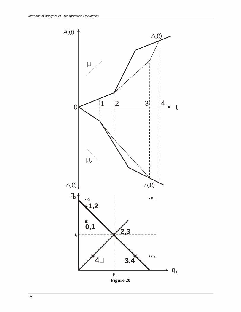
Let us consider the cumulative count diagram of Figure 20, which at this point is assumed only

to include the displayed arrival curves, A1(t) and A2(t). These curves have been plotted opposite

each other using both sides of the ordinate axis. We are also given the outflow diagram included


34

on the bottom right part of the figure, without the dots, which are part of the solution. Note that

µ1 = µ2, and that these rates are shown on the cumulative diagram. We now construct the

departure curves for both approaches, assuming that the system is initially empty.

From time point “0” to time point “1” on the time scale the system remains empty since the

combined arrival rates are less than µ. Thus, the outflows equal the inflows during this period.

This is indicated on the outflow diagram by the point labeled “0, 1”. Note that it is below the

capacity line, as required. There are no queues.

At time point “1” however, the arrival rate “2” goes up to a value equal to 2µ2. This value is

determined graphically by measuring the slope of the arrival curve, and the result is reflected in

our procedure by the point labeled a1 on the outflow diagram. Since there are no queues (yet) we

see from Figure 19 that the outflow point must be directly below this point on the capacity line.

This is point “1, 2” of the diagram, whose coordinates are the outflow rates used for the time

interval after time point “1” on the cumulative plot.

This state of affairs lasts until time point “2” when the inflow on the non-queued approach

suddenly jumps to a value of 2µ1. Again, this is measured from the slope of the arrival curve on a

cumulative count diagram. Because approach 2 already has a queue, we pretend that its desired

inflow is µ and this identifies point a2 on the figure. The recipe of Figure 19 now yields point “2,

3”, whose coordinates are used as the new outflows in the continuation of our departure curves.

Daganzo and Newell

35

The new state of affairs now continues until queue “2” dissipates at time point “3”. Without a

queue, the inflow from approach “2” is now reduced to a level µ2/2. Because approach 1 still has

a queue we pretend, as before, that its desired arrival rate is µ and identify point a3 on the figure.

The procedure of Figure 19 now yields point “3, 4” whose coordinates are again used in the

continuation of the cumulative departure curves.

The new state of affairs ends at time “4” when both queues have dissipated. The final state, after

time “4” includes no queues and is identified by the point “4→” on the outflow diagram.

It is my hope that the concepts learned from this brief explanation will allow you to solve other

problems, and also understand why the solution should be as we have proposed. Good luck in the

lab!


36

A t1( )

A t2( )

t

µ1

µ2

A t1( )

A t2( )

0 1 2 3 4

µ1

µ2

a1

a3

a2

q1

q2

2,3

1,2

0,1

3,44

Figure 20

Daganzo and Newell

37

3. TIME SPACE DIAGRAMS

While queueing theory is a tool designed to study congestion at one point, the time-space

diagram is geared to study movement and how transportation vehicles interact in going from

point to point. This chapter covers the time-space diagram and its transportation applications in

three parts. First, we study the movement of a single vehicle; next, we look at streams of vehicles,

and finally at some highway and public transportation applications.

3.1 Analysis of Vehicular Movement (One Vehicle)

It is useful to start with the case of one vehicle because this will enable us to illustrate

some essential points about the trajectories of vehicles on a time-space diagram. It will then be

easy to generalize the analysis to an arbitrary number of vehicles.

We analyze the one-dimensional movement of vehicles by plotting distance vs. time and

by recording on the graph the position of the front end of the vehicle at different points in time.

When, for one given vehicle, all such positions are connected by a continuous line we say that

we have obtained the trajectory of the vehicle.

Figure 21 depicts the trajectory of a vehicle that is moving, stops and then reverses

directions:


38

Figure 21

The trajectory of a vehicle in a time-space diagram can sometimes be represented by an

analytical function, X(t). If this is not possible, one can study them graphically.

The speed of a vehicle is given by

)(tXdt

dX &=

and its acceleration by

)(2

2

tXdtdX &&=

Thus the shape of the trajectory reveals information about a vehicle’s speed and acceleration. A

constant speed trajectory is a straight line (what would a constant acceleration trajectory by?).

The slope of the line represents the speed (thus a stopped vehicle is represented by a horizontal

segment) and the curvature is related to the acceleration. An accelerating vehicle is represented

as a curve which bends upward (increasing slope when we move from left to right) and a

decelerating vehicle by a curve bending downwards.

Daganzo and Newell

39

If the position of a vehicle’s front end at all points in time is not known one can still

obtain the trajectory of a vehicle from information on its speed and acceleration. Analyses of this

nature are important in accident analyses. In such cases one sometimes is given the length of a

skid mark and is asked to obtain the speed of the vehicle at the time when the brakes were

applied. Except in very simple cases, this involves a time-space analysis where the acceleration

of the vehicle is known (it is equal to the friction factor between the tire and the roadway

adjusted for grade and, perhaps, other factors) and one obtains the trajectory of the vehicle. The

example about to be worked out illustrates the technique.

Example

At time t = 0 a vehicle is stopped at an entrance ramp to a freeway and the driver of such

vehicle observes a platoon of vehicles at a distance X0, coming towards the ramp at a speed V.

Assuming that the stopped vehicle can accelerate uniformly (at a rate, a) from 0 to V, find the

latest time at which the vehicle can safely start the merging maneuver. For simplicity we assume

that the physical dimensions of the vehicle can be neglected.

Solution:

We first draw a time-space trajectory of the freeway platoon and two possible trajectories

of the stopped vehicle:


40

Figure 22

From the figure we conclude that if the vehicle starts at the latest possible time its trajectory will

be tangent to the straight line above (i.e., they will both have the same slope at the point of

intersection). We let τ denote the abovementioned latest possible time.

The trajectory of the accelerating vehicle can be obtained by integrating:

;2

2

adtXd

=

One gets

X = C1 + C2t +at2/2

Since X(τ) = 0 and 0)( =τX& , the constants C1 and C2 are such that:

2)(2

τ−= ta

X

We must find the value of τ such that this trajectory has a slope equal to V when it meets

X = - X0 + V ⋅ t.

Daganzo and Newell

41

The slope equals V if:

a(t - τ) = V

or

t = v/a + τ.

At this point both trajectories must intersect (they are tangent) so:

aV

VX

aVa

aVVX

220

2

0 −=⇒⎟⎠⎞

⎜⎝⎛ −+=⎟

⎠⎞

⎜⎝⎛ ++− ττττ

Negative τ’s indicate that it is too late to attempt a safe merging maneuver.

In some cases it may be necessary to solve a differential equation. This happens when the

acceleration is a function of the position of the vehicle, a(x), or of the speed of the vehicle, a(v).

The former occurs when vehicles are traveling on vertical curves and the latter when vehicles

have an acceleration profile that depends on speed (which is almost always the case). The

differential equations are:

)( and

)(

2

2

2

2

vadtxd

xadtxd

=

=

In both cases one can use the change of variable

dxdvV

dtdx

dxdV

dtdV

dtXd

⋅=⋅=

=2

2


42

In the first case one solves VdV = a(x)dx by integrating on both sides. Once V(x) is obtained, one

gets the trajectory by solving dx/V(x) = dt by integration. The trajectory X(t) will contain two

integration constants which must be obtained from boundary conditions.

In the former case the equation becomes VdV/a(V) = dx which after integration on both

sides yields V(x). The rest of the procedure is the same as in the first case.

3.2 Analysis of Vehicular Movement (Several Vehicles)

The time-space diagram provides a natural way of keeping track of the positions of

several vehicles at the same time. It is therefore very valuable in order to study the vehicular

intersections that might arise.

A time-space diagram containing the trajectories of several vehicles can be regarded in an

interesting way. Assume that we take aerial photographs of the road at constant intervals of times

t1, t2, etc., and that in these photographs vehicles are represented as dots (see Figure 23).

Daganzo and Newell

43

Figure 23

If we put these photographs together side by side at equally spaced distances and connect the

dots by smooth curves, we obtain a time space diagram:

Figure 24


44

Thus vertical slices of the time-space diagram represent instantaneous pictures of the road. As a

matter of fact, if we looked through a vertical thin slice at the time-space diagram and moved the

slit from left to right, we would see an aerial movie of the vehicular movement on the road!

It should be clear at this point that intersecting trajectories represent passing vehicles (or

crossing if one trajectory is ascending and the other one is descending). Of course, in narrow

roads where passing is not possible, time-space diagrams cannot have intersecting trajectories.

This is a feature of the time-space diagram that makes it very useful for scheduling trains and

other transportation modes over a single track rail.

Before looking at those problems, we consider some macroscopic measures of vehicular

flow on roads and derive some useful relationships among these.

3.3 The Fundamental Relationship of Flow and the Fundamental Diagram

Let us define the following terms:

Headway = the time elapsed between the passage of consecutive vehicles (their front ends) as seen by a bystander.

Spacing = the front end to front end distance in between two cars at a given instant.

Volume (q) = the number of vehicles observed by a bystander at a certain location divided by the time interval.

Density (k) = the number of vehicles over a small section of a road at a given instant divided by the length of the section.

Daganzo and Newell

45

Figure 25 illustrates these concepts:

Figure 25

The following relationships are important:

headwayqspacingk

/1/1

≈≈

The first one is true because the average spacing, spacing, is by definition:

kspacing 1

vehiclesofNumber sby vehicle occupiedLength

vehiclesofNumber spacings

=== ∑

The relationship is exact only if the portion of the road over which k is measured coincides with

the length occupied by the vehicles (i.e., if there is a vehicle at both the beginning and end of the

portion of road). The second relationship is analogously true.

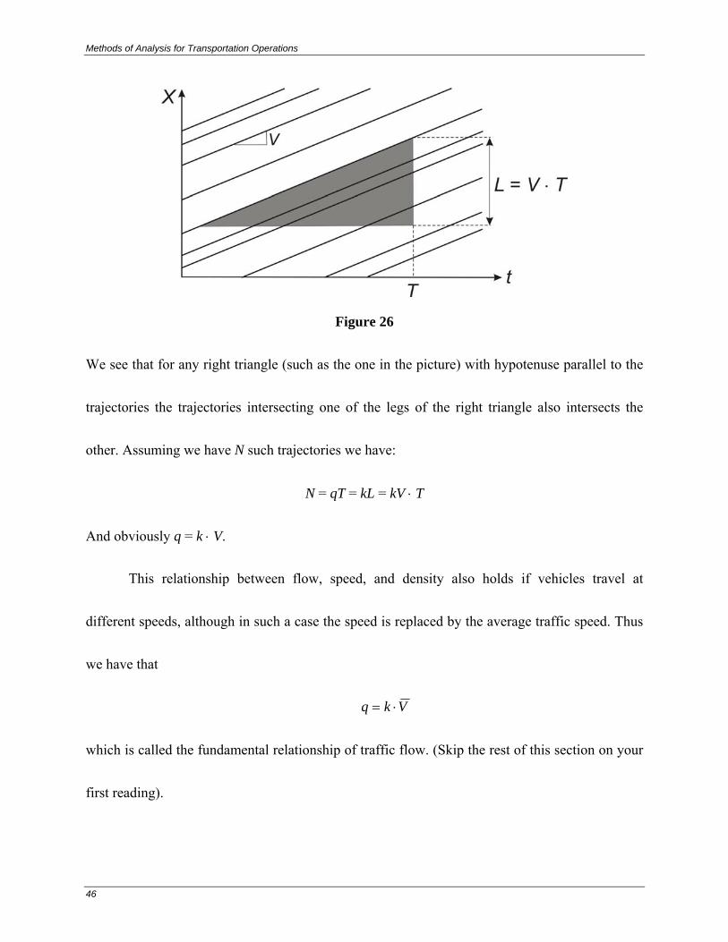
For vehicles going at a speed V the time-space diagram looks like Figure 26.


46

Figure 26

We see that for any right triangle (such as the one in the picture) with hypotenuse parallel to the

trajectories the trajectories intersecting one of the legs of the right triangle also intersects the

other. Assuming we have N such trajectories we have:

N = qT = kL = kV ⋅ T

And obviously q = k ⋅ V.

This relationship between flow, speed, and density also holds if vehicles travel at

different speeds, although in such a case the speed is replaced by the average traffic speed. Thus

we have that

Vkq ⋅=

which is called the fundamental relationship of traffic flow. (Skip the rest of this section on your

first reading).

Daganzo and Newell

47

If we have families of vehicles going at different speeds (the parameters qi, ki, and Vi identify

a family) one has that

qi = kiVi

and summing both sides over all families

si

iii

ii Vk

kk

VkVkq ×=⎟⎠⎞

⎜⎝⎛== ∑∑

Note that ⎟⎠⎞

⎜⎝⎛=

kk

VV iis is the average speed of the vehicles that would appear on an

aerial photograph. It is called the space mean speed.

The average speed observed by a bystander is

∑ ⎟⎟⎠

⎞⎜⎜⎝

⎛=

i

iit q

qVV

(the speed of each family weighed by the relative frequency of observation). It is called the

time mean speed.

Although, for most transportation systems sV and tV are practically the same

(difference less than 5%), it turns out that tV is always larger than sV . This is easy to see

because if Vi > Vj,

⎟⎟⎠

⎞⎜⎜⎝

⎛>⎟

⎟⎠

⎞⎜⎜⎝

⎛⎟⎟⎠

⎞⎜⎜⎝

⎛=⎟

⎟⎠

⎞⎜⎜⎝

⎛

j

i

j

i

j

i

j

i

kk

VV

kk

qq

and thus, higher speeds are more heavily weighted when one calculates tV than when one

calculates sV .


48

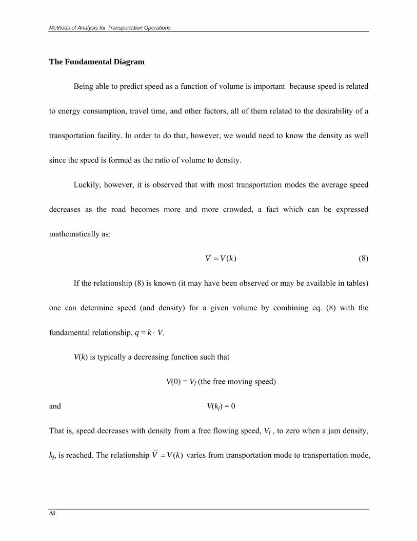
The Fundamental Diagram

Being able to predict speed as a function of volume is important because speed is related

to energy consumption, travel time, and other factors, all of them related to the desirability of a

transportation facility. In order to do that, however, we would need to know the density as well

since the speed is formed as the ratio of volume to density.

Luckily, however, it is observed that with most transportation modes the average speed

decreases as the road becomes more and more crowded, a fact which can be expressed

mathematically as:

)(kVV = (8)

If the relationship (8) is known (it may have been observed or may be available in tables)

one can determine speed (and density) for a given volume by combining eq. (8) with the

fundamental relationship, q = k ⋅ V.

V(k) is typically a decreasing function such that

V(0) = Vf (the free moving speed)

and V(kj) = 0

That is, speed decreases with density from a free flowing speed, Vf , to zero when a jam density,

kj, is reached. The relationship )(kVV = varies from transportation mode to transportation mode,

Daganzo and Newell

49

it depends on the type of facility under consideration and ton environmental conditions. The first

relationship ever introduced was proposed for highway traffic and was a linear function:

⎟⎟⎠

⎞⎜⎜⎝

⎛−=

jf k

kVV 1 (9)

This relationship was fitted to data by using linear regression.

The important thing is that equations (7) and (8) (or (9)) give two relationships between

three variables, thus one can always express two as a function of the other one. The two most

common ways of doing that is by plotting volume vs. speed and density vs. volume.

We first note that for any given density one can write:

Q = V ⋅ k = kV(k)

and that q = 0 if either k = 0 or k = kj. Since, for values of k between zero and kj, q is positive the

k – q relationship must reach a maximum for some k = kop (optimal density). See the figure

below (ignore the dotted line):


50

Figure 27

The maximum qmax is called the capacity. The q vs. k diagram is very useful because in it

the speed is given by the slope of the line connecting a point on the diagram to the origin of

coordinates (see dotted line on the figure and remember that V = q/k). The diagram, thus relates

the three fundamental variables. Because of this, it is termed the fundamental diagram.

It is sometimes convenient to have flow vs. speed on a diagram, especially when one is

not interested in density. The flow vs. speed diagram looks like the one below:

Daganzo and Newell

51

Figure 28

Note that for every value of flow there are two values of speed. As an exercise, find the

equation of the k – q and v – q curves for the linear model of equation (9); also find the values of

kop, Vop, and qmax.

If we distinguish between scheduled (transportation modes such as trains, buses, etc.,

whose frequency (volume) and speed is decided by a central authority or dispatcher) and

unscheduled modes (modes such as automobile, bicycle, and foot transportation) we note that for

the latter the operating speed is set by the vehicles themselves and that only the top part of the q

– V curve is actually meaningful. Traffic will operate on the bottom part of the curve whenever a

restriction (i.e., an accident, slow-moving truck, etc.) forces traffic to move at a speed smaller

than Vop. However, when that restriction is removed traffic accelerates (the dynamics of this


52

phenomenon are complicated and will not be explored in this course) and return to the normal

operating point on the top part of the curve.

For unscheduled modes it, thus, suffices to consider (for most purposes) the half

diagrams below:

Figure 29

The Highway Capacity Manual (Ref. 3) which is extensively used by Traffic Engineers

contains extensive tables and figures with q – v curves for all types of highway facilities.

Scheduled transportation modes can operate on any point of the curve (it is the decision

of the central dispatcher) as it is seen in the next section, they can also operate in the region

inside the curve.

With scheduled transportation modes the operating characteristics (q, k, and V) can be

decided by the central controller, of course, subject to their satisfying q = k⋅V.

For scheduled modes the three terms in this formula mean: q (frequency); k (number of

vehicles/length of route); V (average speed including stops).

Daganzo and Newell

53

In public transportation systems, for instance, one can select the density, k, by fixing the

number of buses on a line; one can also (to a certain extent) fix their average round-trip speed by

providing different numbers of stops. Once this is done, the frequency of service, q, is

automatically fixed.

The values of k and V, however, cannot be arbitrarily selected because of safety reasons.

For a certain value of k, there is a value V(k) which cannot be exceeded; this relationship is

analogous to the one in the previous section and, thus, defines a fundamental diagram; i.e., for

any given k we can find V(k) and q = kV(k), the maximum safe speed (including stops) and flow.

However, since speeds smaller than V(k) are also safe, (q, k, u) combinations in the shaded area

(see Figure 30) are also feasible.

Figure 30

The density-volume diagram for railroads operating on a single track with a Block Signal

Control System (a system of traffic lights that always ensures a minimum distance, b, between


54

the rear end of a train and the beginning of the next one) is obtained as an example. We assume

that there are no stops.

We know that the spacing between trains must be larger than the length of a train, ℓ, and

the block distance, b; thus:

spacing ≥ b + ℓ

and k ≤ 1/( b + ℓ).

The maximum safe operating speed of the trains is selected to ensure that a train can

brake to a stop in less than b distance units. For this example, we will assume that the train must

be able to stop in b/2 distance units.

It is well known that the braking distance of a moving object at a constant deceleration

rate, f ⋅ g, (f is the coefficient of friction and g the acceleration of gravity) is:

)(2 distance braking

2

gfV⋅

=

This formula can be obtained with the methods in Section 3.1. For safety we have:

22

2 bfg

V<

and gfbV ⋅⋅<

The diagram and set of possible operating points for a block length, b, is:

Daganzo and Newell

55

Figure 31

One can now explore what happens to the maximum operating speed, density and flow (point P

above) when the block length, b, and/or the length of the trains is changed.

The same type of analysis can be carried out when there are stops on the way; however in

that case it is more convenient to obtain the maximum flow directly from the time-space diagram.

The diagram below depicts the time-space trajectories of two consecutive trains as they stop at

two contiguous stations:

Figure 32


56

It can be seen that the trajectory of the following train is identical to the trajectory of the first

train but shifted to the right by an amount: d + (b + ℓ)/V′.

This is the minimum safe headway and, thus, the maximum frequency is:

dVbV

Vbd

q′++

′=

′+

+=

ll

1max

The time-space diagram is very useful to analyze situations where the trajectory of one

vehicle is affected by the trajectory of other vehicles. The uses of the time-space diagram are

best explained by means of examples. The next section provides some solved problems (some of

which have appeared in previous exams) covering the material in this chapter and illustrating

different uses of the time-space diagram.

3.4 Examples

Problem 1

Rapid transit service is offered on a 40 km long (round trip) route with a total of 10 stops

(one stop every 4 km). Trains stop at the stations for 30 sec. If the average speed of the trains

excluding stops is 80 km/hr, calculate the maximum possible frequency and the required number

of trains if trains must be separated at all times by at least 1 km and they are 200 m long.

Daganzo and Newell

57

Solution:

From a time space diagram such as the last one, we find that

The average speed of the trains is

km/hr 57.68

36003010

8040

40Time Trip Round

40=

×+==V

and the density 625.057.6886.42max ===

Vq

k

The number of trains is N = k × 40 = 25.

At this point we note that instead of q = V ⋅ k we could have used (this is always possible

for public transportation) q = N/(Round Trip Time) since

LengthVehicles ofNumber and

Time TripLength

== kV

Problem 2

We now study a one-way railroad without stops. Assuming that the top speed of a train is

V* (a function of the length of the train and the number and power of the engines) find the block

length that allows the largest possible frequency.

Solution

We first note that V ≤ V* and gfbV ⋅⋅≤ . Thus:

{ }gfbVV ⋅⋅≤ ∗ ;min

veh/hr86.42

360030802.01

80max =

×++=

′++′

=dVb

Vql


58

and l+

≤b

k 1 .

As was discussed before, qmax (the ordinate of point P in the figure before the last one) is

given by:

{ }⎪⎭

⎪⎬⎫

⎪⎩

⎪⎨⎧

+⋅⋅

+=

+⋅⋅

=∗∗

lll bgfb

bV

bgfbV

q ;min;min

max

We shall find the value of b that maximizes qmax. Let b0 be the value of b that makes

gfbV ⋅⋅=∗ ; i.e., fg

Vb2*

0 = . The function

l+⋅⋅

=b

gfbqmax

has a maximum (you should check this by taking derivatives) for b = ℓ (which is also the sought

maximum if ℓ < b0…Case II in the figure below).

If ℓ > b0 the plot of qmax vs. b has the maximum at b = b0 (see also the figure below).

Figure 33

The solution can be written more concisely as: b = min{b0, ℓ}.

Daganzo and Newell

59

Problem 3

This problem illustrates the use of the time-space diagram to analyze the interaction of

vehicles in a narrow way.

Figure 34

The above waterway is wide enough for one ship only, except in the central siding which is wide

enough for two ships. Ships can travel at an average speed of six miles/hour; they must be spaced

at least one-half mile apart while moving in the waterway and 0.25 miles apart while stopped in

the siding. Westbound ships travel full of cargo and are thus given high priority by the canal

authority over the eastbound ships which travel empty.

Westbound ships travel in four ship convoys which are regularly scheduled every 3-1/2

hours and do not stop at the siding.

1. Find the maximum daily traffic of eastbound ships.

2. Find the maximum daily traffic of eastbound ships if the siding is expanded to one

mile in length on both sides to a total of three miles.


60

Note: We assume that eastbound ships wait exactly six minutes to enter either one of

the straightaways after a westbound convoy has cleared it. We do this to take

into account that ships do not accelerate instantaneously.

Solution

We first draw the time-space diagram for the problem at an adequate scale. Next, we plot

the trajectories of the high-priority (westbound) convoys. These have been plotted in the figure.

The dashed band (width – one mile) represents the siding where eastbound and westbound

trajectories may cross. These dashed lines will help us draw the eastbound trajectories.

Part 1:

We start by drawing the trajectory of a ship entering the western end of the canal at 3:30

p.m. (the earliest possible time for that particular gap in between convoys). Note how it must

stop at the eastern end of the siding to yield the right of way to the last ship of the westbound

convoy; note also how it makes it within the 5 min allowance to the eastern end of the canal. The

same process is followed successfully with the second trajectory. In that case we must also watch

for the safe spacings while moving and stopped. The third ship, however, would not be able to

arrive to the western end of the siding within the 5 min allowance and it cannot be dispatched.

Capacity = 2(ships per 3-1/2 hours) × ships/day 71.13hours

213

(hours) 24=

Daganzo and Newell

61

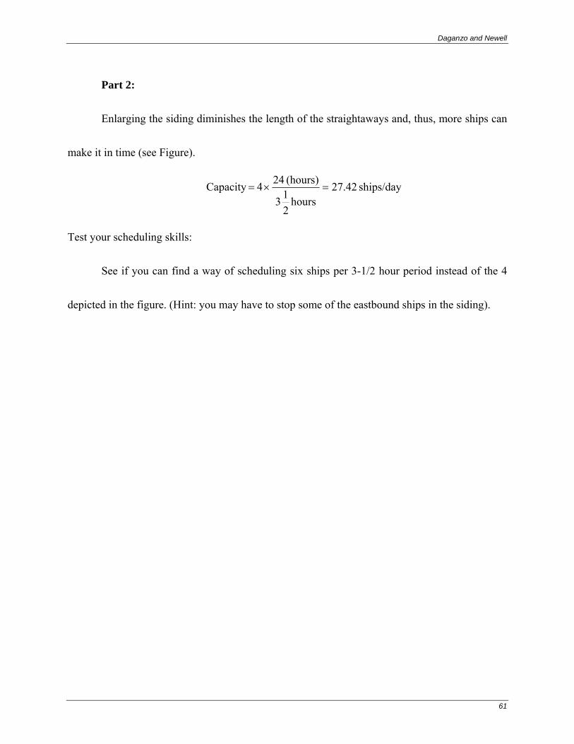
Part 2:

Enlarging the siding diminishes the length of the straightaways and, thus, more ships can

make it in time (see Figure).

ships/day 42.27hours

213

(hours) 24 4 Capacity =×=

Test your scheduling skills:

See if you can find a way of scheduling six ships per 3-1/2 hour period instead of the 4

depicted in the figure. (Hint: you may have to stop some of the eastbound ships in the siding).


62

`

0

1

2

3

4

5

6

7

8

9

10

11

12

13

14

15

16

17

18

19

0 1 2 3 4 5 6 7 8Time (hours)

Figure 35

1 mile wide

East

West

Daganzo and Newell

63

0

1

2

3

4

5

6

7

8

9

10

11

12

13

14

15

16

17

18

19

0 1 2 3 4 5 6 7 8Time (hours)

Figure 36

3 miles wide

East

West


64

4. MODELLING ENERGY, AIR POLLUTION AND NOISE

In addition to travel time, there are some other characteristics of transportation systems

that have an impact on non-users of the system, as well. A limited list would include: energy

consumption, land consumption, consumption of construction materials, air pollution, noise,

water pollution, soil erosion, effects on land use, etc.

Some of these transportation impacts are principally caused by the existence of the

transportation facility itself. Others are also dependent on the amount of transportation activity

taking place on and around the facility under consideration. The former impacts are easier to

assess than the latter ones and they also appear (at least most of them) in the construction of

other civil engineering structures. Because of this, they will not be covered in this brief review.

We concentrate on the other impacts (i.e., energy consumption, air pollution, and noise).

Although land use is related to traffic this relationship is beyond the scope of this discussion.

The same modelling approach can be used to study energy, pollution and noise. In this

handout, we concentrate on microscopic studies (i.e., studies involving a single transportation

facility) rather than on macroscopic studies involving an entire town, region or country. The

latter are much more difficult to study and they require a thorough understanding of the

microscopic scene.

Daganzo and Newell

65

4.1 The Modelling Philosophy

Three important steps are involved:

Step 1: Analyze the facility under consideration for the desired period of time by means of a queueing or time-space diagram depending on the case.

Step 2: Look at the number of stop and go maneuvers, average speed, total amount of time spent by all vehicles in the facility. (In some cases, it may also be desirable to know the average acceleration of a typical vehicle).

Step 3: From the numbers calculated in Step 2, obtain the energy consumed, the air pollution generated, and the noise. This is done by means of empirical formulae which relate the number of stops, speeds, etc. to the dependent variables. It must be born in mind, however, that the state-of-the-art in this area is very primitive and that good judgment plays an important role since few formulas are available.

We now review what little is known about these formulas for each one of the impacts.

4.2 Energy Consumption

Transportation modes consume energy at different rates depending on the speed,

acceleration, and grades. For instance, for transit vehicles, railroads and other land vehicles, the

power (energy/unit time) consumed can be expressed as:

P = (k1 + k2V + k3V2)vW + V(grade)W + Vga W


66

where V is the speed, a is the acceleration, g is the acceleration of gravity and W is the weight of

the vehicle. The first term is due to the rolling and air friction, the second term to the grade and

the last term to the acceleration of the vehicle.1

It is easy to obtain from the time-space trajectory of a vehicle the total energy consumed

by measuring the speeds and accelerations on the graph.

For transit vehicles which stop at stations, a simpler formula (somewhat less accurate)

can be used for the energy consumed on a round trip.

E = f(V)LW + k4Ns

where V is the cruising speed, L is the route length and Ns is the number of stops. Although this

formula seems to neglect the effects of grade and the accelerations and deceleration maneuvers

due to traffic, both of these can be captured to a certain extent by proper selection of f(V) and k4.

The formula, however, is much simpler to apply than the one above. It can also be used for

highway vehicles provided one knows the average number of deceleration/acceleration

maneuvers (Ns) and the characteristics (maximum and minimum speeds) of a typical

deceleration/acceleration cycle. (Ref. 4, pp. 27 and on, contains data on fuel consumption and

speed of highway vehicles).

1 One must bear in mind that, except for electric engines which can recover and store the braking energy, values of P

smaller than zero cannot occur because braking transforms the kinetic energy into heat which dissipates. One must,

thus, use P = 0 whenever the calculated value is smaller than zero.

Daganzo and Newell

67

For very slow traffic (average speed under 40 mph), the following amazingly simple

formula has been obtained and shown to be accurate by a group of researchers at General

Motors:

E = k5L + k6T

The gasoline consumed on a trip in an urban area is a linear function of distance and

travel time! Typical values of k5 and k6 for automobiles are:

k5 = 90 ml/km k6 = 0.44 ml/sec.

4.3 Air Pollution

Air pollution is a much more complicated problem than energy consumption because

different pollutants are emitted at different levels by different engines at different speeds.

However, the same modeling approach as was used with energy can be used.

For instance the emissions of NOx increase with low air/fuel ratios but those of

hydrocarbon decrease. Typical curves for an internal combustion engine (auto) would be:


68

Figure 37 Relationship of typical engine emissions and performance to the air/fuel ratio. (The vertical scale is linear and shows relative values for each parameter. Stoichiometric—in proportion exactly right for a specific chemical reaction with no excess of any reactant or product.)

Chapter 21 on Ref. 4 contains more data on emissions vs. speed.

However, even if one succeeds in predicting the total amount of pollutants that are

discharged into the atmosphere, it would still be necessary to assess how fast these pollutants are

diffused through the atmosphere. This is because pollution effects are most damaging when they

are highly concentrated in a few places rather than uniformly spread over a large area.

Daganzo and Newell

69

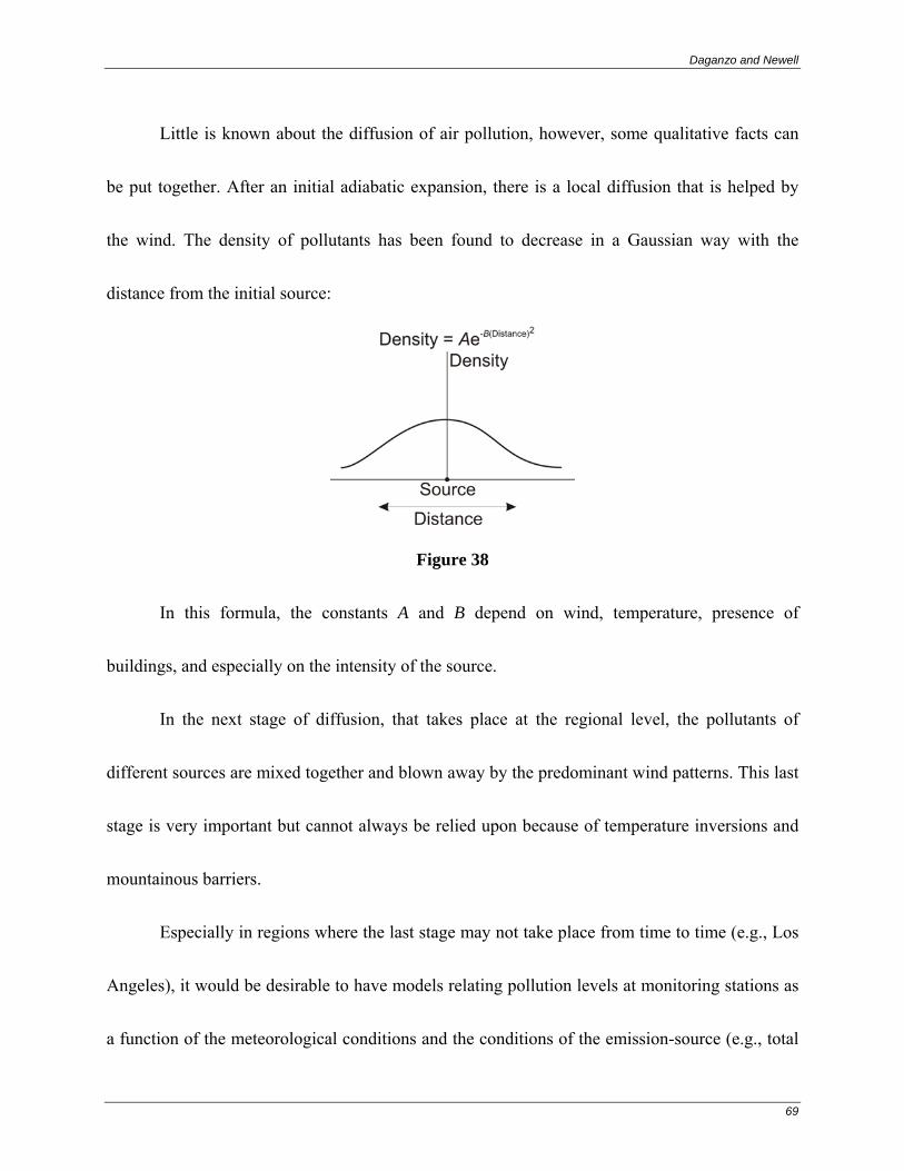
Little is known about the diffusion of air pollution, however, some qualitative facts can

be put together. After an initial adiabatic expansion, there is a local diffusion that is helped by

the wind. The density of pollutants has been found to decrease in a Gaussian way with the

distance from the initial source:

Figure 38

In this formula, the constants A and B depend on wind, temperature, presence of

buildings, and especially on the intensity of the source.

In the next stage of diffusion, that takes place at the regional level, the pollutants of

different sources are mixed together and blown away by the predominant wind patterns. This last

stage is very important but cannot always be relied upon because of temperature inversions and

mountainous barriers.

Especially in regions where the last stage may not take place from time to time (e.g., Los

Angeles), it would be desirable to have models relating pollution levels at monitoring stations as

a function of the meteorological conditions and the conditions of the emission-source (e.g., total


70

vehicle miles of travel). It would then be possible to operate the transport system rationally to

avoid dangerous pollutant levels. This is, however, still some time away in the future.

4.4 Noise

Noise from transportation vehicles is a function of the vehicle operating characteristics

and of its interaction with the way. Noise is measured in decibels (db) which are related to the

logarithm of the sound pressure.

The meaning of decibels can be seen from the table below:

Figure 39

4.4.1 Attenuation with Distance and Addition Rules

Noise levels diminish with distance from the noise source. They diminish in different

ways depending on the type of source. A point source generates spherical sound waves which

cause the decibels to decrease by 6 dB every time the distance is doubled. For a line source

Daganzo and Newell

71

(e.g., traffic on a crowded highway) the sound wave is cylindrical and the sound level decreases

by 3 dB every time the distance is doubled. Some transportation sources such as transit t rains

are neither point nor line sources (they are segment sources); in these cases, empirical studies

have shown that for distances smaller than 0.3 times the length of the source, the source behaves

as a point source and for larger distances as a line source.

Another complicating characteristic of noise is the way in which it is compounded. If L1

and L2 are the decibel levels of two sources at a point P, the combined effect of both sources,

LSUM, is not L1 + L2 but rather:

( )[ ]10/101

211.01log10 LLSUM LL −++=

This formula behaves peculiarly in the sense that it is always more effective to reduce the level

of the loudest noise source.

Example:

A motorcycle generates noise of 90 dB at 15 m. The general traffic noise background is

80 dB. Clearly the combined noise is 90.41 dB.

You must check by using the above formula that reducing motorcycle noise by 5 dB

results in a 4.21 reduction in total noise and that a 5 dB reduction in traffic noise results in a total

reduction of 0.28 dB.

4.4.2 Noise Models


72

Because of these complicated rules and because noise can be reflected in different

amounts of surfaces such as buildings and tree branches, it is difficult to predict the noise impact

of a new facility, especially since different sources generate noises of different frequencies and

in different directions.

Nevertheless, some empirical models have been developed for highways which give the

noise level as a function of traffic speed and volume (note how in the case of noise it is also

important to obtain information on the operating characteristics of the stream). The following

formula gives the decibel level:

29)]00119.0[tanh(log10log20log15log10 10101010 +++−=VqdVdqL

The units in this formula are: q (vph); d (distance in feet); and V (mph).

For air transportation (as happens with transit, as well) volume and speed are not

important since the source of problems is the small volume of very large aircraft (some

exceeding the sound barrier). Studies in these cases concentrate on the noise emission

characteristics of individual vehicles when operating close to densely populated areas.

Daganzo and Newell

73

REFERENCES

1. Gordon F. Newell, Applications of Queueing Theory, Chapman and Hall, 1971.

2. D.R. Cox and Walter L. Smith, Queues, Chapman and Hall, 1971.

3. Highway Capacity Manual, Highway Research Board Special Report 87, 1965.

4. Transportation Engineering Handbook, Institute of Transportation Engineers, Prentice

Hall, 1976.

methods of analysis - robert l. bertinibertini.eng.usf.edu/courses/559/methods_of_analysis.pdf ·...

Documents