TKT-2546 Methods for Positioning

Jussi CollinHelena Leppäkoski

Martti Kirkko-Jaakkola

2010

Preface

This hand-out continues the hand-out of the course MAT-45806 Mathematics for Positioning(http://math.tut.fi/courses/MAT-45806/). These courses are closely related and used toshare the same hand-out in the past years. This year, however, each course has its own hand-out.Mathematics for Positioning is a highly recommended but notmandatory prerequisite for thiscourse.

The purpose is that Mathematics for Positioning presents mathematical principles and concepts,particularly statistics and optimization, lying under many positioning methods. In this course,these tools are applied to practical positioning problems.

Any errata found in the text will be reported on the course website athttp://www.tkt.cs.tut.fi/kurssit/2546/.

We would like to thank Simo Ali-Löytty, Niilo Sirola, and Henri Pesonen especially for devel-oping the LATEX template used for this hand-out. Furthermore, Hanna Sairois acknowledgedfor her contributions in the previous versions of the hand-out, based on which the beginning ofChapter 2 has been rewritten.

Tampere, 19 Feb 2010

authors

2

Contents

1 Sensor-Assisted Positioning 41.1 Accelerometers and Gyroscopes . . . . . . . . . . . . . . . . . . . . .. . . . 41.2 Odometers . . . . . . . . . . . . . . . . . . . . . . . . . . . . . . . . . . . . . 71.3 Altitude Measurement . . . . . . . . . . . . . . . . . . . . . . . . . . . . .. 81.4 Sensor Measurement Errors . . . . . . . . . . . . . . . . . . . . . . . . .. . . 9

2 Carrier Phase Based Satellite Positioning 152.1 Doppler Effect . . . . . . . . . . . . . . . . . . . . . . . . . . . . . . . . . . .152.2 Differential Positioning . . . . . . . . . . . . . . . . . . . . . . . . .. . . . . 182.3 Real-Time Kinematics . . . . . . . . . . . . . . . . . . . . . . . . . . . . .. 21

3 Integrity and Reliability 273.1 Positioning Performance Metrics . . . . . . . . . . . . . . . . . . .. . . . . . 273.2 Statistical Inference and Hypothesis Testing . . . . . . . .. . . . . . . . . . . 303.3 Residuals . . . . . . . . . . . . . . . . . . . . . . . . . . . . . . . . . . . . . 353.4 Receiver Autonomous Integrity Monitoring . . . . . . . . . . .. . . . . . . . 373.5 Reliability Testing Based on Global and Local Tests . . . .. . . . . . . . . . . 39

Index 46

References 48

3

Chapter 1

Sensor-Assisted Positioning

JUSSI COLLIN

Because of the very low transmit power of satellite signals,users frequently encounter situationswhere a position solution is not available. For example, underground parking lots and shoppingmalls are places where an accurate position solution could be quite useful but a GPS receiverdoes not help. In such places, e.g., a WLAN network can enableradiolocation. However, adevice equipped with proper sensors can obtain informationabout the motion of its user withoutany external help. In this chapter, sensors suitable for positioning are presented. Furthermore,resolving the user positioning using sensor information isaddressed, and finally, some simplesensor error models are discussed.

Coordinate frame transformations were studied in the course “Mathematics for Positioning” [2,Chapter 1], and basically, sensor positioning algorithms are based on these operations: first,measure the change in position in the device body frame; then, transform the measured changeto the navigation frame; finally, integrate to obtain the position. This procedure yields a route onthe map, as long as the initial position is obtained from someother source. In practice, externalaiding is required more frequently than once due to the accumulation of biases in integration.

1.1 Accelerometers and Gyroscopes

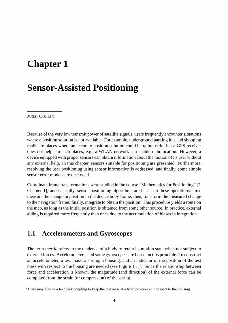
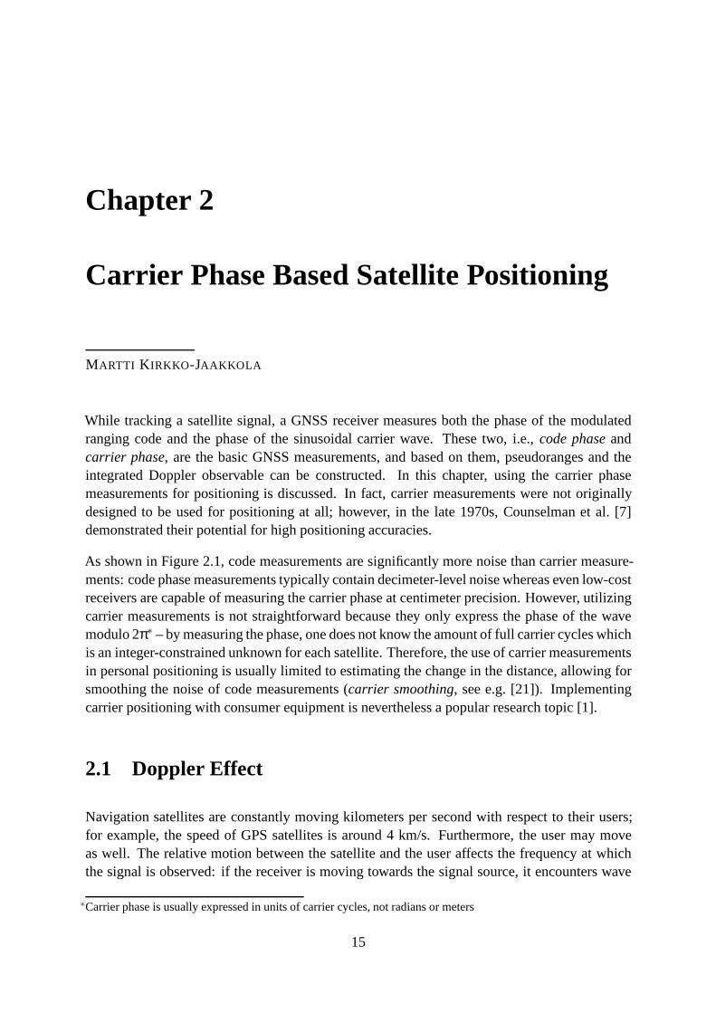
The terminertia refers to the tendence of a body to retain its motion state when not subject toexternal forces. Accelerometers, and some gyroscopes, arebased on this principle. To constructan accelerometer, a test mass, a spring, a housing, and an indicator of the position of the testmass with respect to the housing are needed (see Figure 1.1)∗. Since the relationship betweenforce and acceleration is known, the magnitude (and direction) of the external force can becomputed from the strain (or compression) of the spring.

∗There may also be a feedback coupling to keep the test mass at afixed position with respect to the housing.

4

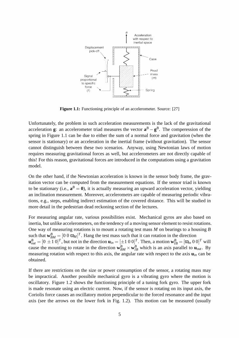
Figure 1.1: Functioning principle of an accelerometer. Source: [27]

Unfortunately, the problem in such acceleration measurements is the lack of the gravitationalaccelerationg: an accelerometer triad measures the vectoraB−gB. The comperession of thespring in Figure 1.1 can be due to either the sum of a normal force and gravitation (when thesensor is stationary) or an acceleration in the inertial frame (without gravitation). The sensorcannot distinguish between these two scenarios. Anyway, using Newtonian laws of motionrequires measuring gravitational forces as well, but accelerometers are not directly capable ofthis! For this reason, gravitational forces are introducedin the computations using a gravitationmodel.

On the other hand, if the Newtonian acceleration is known in the sensor body frame, the grav-itation vector can be computed from the measurement equations. If the sensor triad is knownto be stationary (i.e.,aB = 0), it is actually measuring an upward acceleration vector, yieldingan inclination measurement. Moreover, accelerometrs are capable of measuring periodic vibra-tions, e.g., steps, enabling indirect estimation of the covered distance. This will be studied inmore detail in the pedestrian dead reckoning section of the lectures.

For measuring angular rate, various possibilities exist. Mechanical gyros are also based oninertia, but unlike accelerometers, on the tendency of a moving sensor element to resist rotations.One way of measuring rotations is to mount a rotating test mass M on bearings to a housingBsuch thatwB

BM = [0 0 ωM]T . Hang the test mass such that it can rotation in the directionuB

out = [0 ±1 0]T , but not in the directionuin = [±1 0 0]T . Then, a motionwBIB = [ωin 0 0]T will

cause the mounting to rotate in the directionwBBM ×wB

IB which is an axis parallel touout. Bymeasuring rotation with respect to this axis, the angular rate with respect to the axisuin can beobtained.

If there are restrictions on the size or power consumption ofthe sensor, a rotating mass maybe impractical. Another possibile mechanical gyro is a vibrating gyro where the motion isoscillatory. Figure 1.2 shows the functioning principle ofa tuning fork gyro. The upper forkis made resonate using an electric current. Now, if the sensor is rotating on its input axis, theCoriolis force causes an oscillatory motion perpendicularto the forced resonance and the inputaxis (see the arrows on the lower fork in Fig. 1.2). This motion can be measured (usually

5

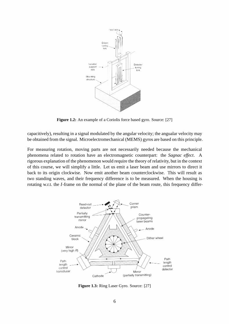
Figure 1.2: An example of a Coriolis force based gyro. Source: [27]

capacitively), resulting in a signal modulated by the angular velocity; the angualar velocity maybe obtained from the signal. Microelectromechanical (MEMS) gyros are based on this principle.

For measuring rotation, moving parts are not necessarily needed because the mechanicalphenomena related to rotation have an electromagnetic counterpart: theSagnac effect. Arigorous explanation of the phenomenon would require the theory of relativity, but in the contextof this course, we will simplify a little. Let us emit a laser beam and use mirrors to direct itback to its origin clockwise. Now emit another beam counterclockwise. This will result astwo standing waves, and their frequency difference is to be measured. When the housing isrotating w.r.t. theI -frame on the normal of the plane of the beam route, this frequency differ-

Figure 1.3: Ring Laser Gyro. Source: [27]

6

ence changes∗. Gyroscopes operating on this principle are called Ring Laser Gyros (RLG);Figure 1.3 is an illustration of an RLG. Optical measurements have various advantages:

• High accuracy.

• Unlimited input bandwidth.

• No moving parts, hence insensitive to vibrations and more reliable than mechanical gyros.

• Unaffected by linear accelerations.

On the other hand, manufacturing costs, size, and power consumption make RLGs infeasiblefor personal applications—at least thus far.

1.2 Odometers

A fundamental problem in acceleration-based displacementmeasurements is double integration:even small biases will accumulate over time. For this reason, sensors measuring the rotation ofthe wheels of a vehicle and other odometers almost invariably perform more accurately. Thelargest error source of odometers is the scale factor: for instance, the radius of a wheel is notprecisely known. In this case, the position error is proportional to the covered distance insteadof time. As opposed to purely inertial measurements, these methods are somewhat dependenton external factors: for example, a slippery road surface may cause wheelspin.

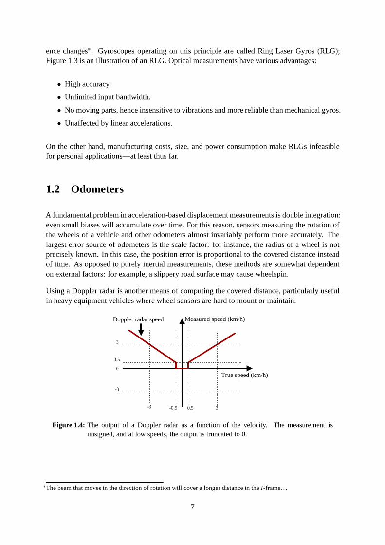
Using a Doppler radar is another means of computing the covered distance, particularly usefulin heavy equipment vehicles where wheel sensors are hard to mount or maintain.

0

3

-3

True speed (km/h)

Measured speed (km/h)

0.5

0.5-0.5 3-3

Doppler radar speed

Figure 1.4: The output of a Doppler radar as a function of the velocity. The measurement isunsigned, and at low speeds, the output is truncated to 0.

∗The beam that moves in the direction of rotation will cover a longer distance in theI -frame. . .

7

1.3 Altitude Measurement

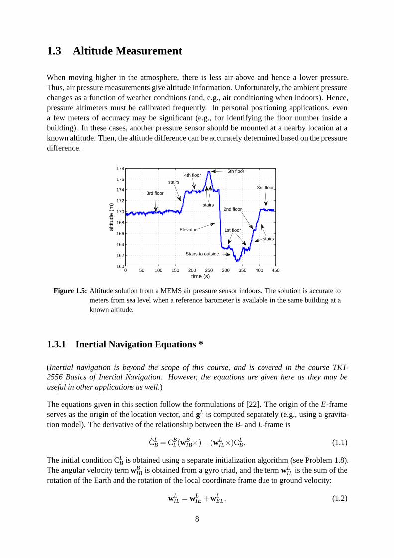
When moving higher in the atmosphere, there is less air aboveand hence a lower pressure.Thus, air pressure measurements give altitude information. Unfortunately, the ambient pressurechanges as a function of weather conditions (and, e.g., air conditioning when indoors). Hence,pressure altimeters must be calibrated frequently. In personal positioning applications, evena few meters of accuracy may be significant (e.g., for identifying the floor number inside abuilding). In these cases, another pressure sensor should be mounted at a nearby location at aknown altitude. Then, the altitude difference can be accurately determined based on the pressuredifference.

0 50 100 150 200 250 300 350 400 450160

162

164

166

168

170

172

174

176

178

altit

ude

(m)

time (s)

stairs

4th floor5th floor

Elevator 1st floor

3rd floor3rd floor

Stairs to outside

stairs

stairs

2nd floor

Figure 1.5: Altitude solution from a MEMS air pressure sensor indoors. The solution is accurate tometers from sea level when a reference barometer is available in the same building at aknown altitude.

1.3.1 Inertial Navigation Equations *

(Inertial navigation is beyond the scope of this course, and is covered in the course TKT-2556 Basics of Inertial Navigation. However, the equationsare given here as they may beuseful in other applications as well.)

The equations given in this section follow the formulationsof [22]. The origin of theE-frameserves as the origin of the location vector, andgL is computed separately (e.g., using a gravita-tion model). The derivative of the relationship between theB- andL-frame is

CLB = CB

L(wBIB×)− (wL

IL×)CLB. (1.1)

The initial condition CLB is obtained using a separate initialization algorithm (seeProblem 1.8).The angular velocity termwB

IB is obtained from a gyro triad, and the termwLIL is the sum of the

rotation of the Earth and the rotation of the local coordinate frame due to ground velocity:

wLIL = wL

IE +wLEL. (1.2)

8

The local frameL retains itsz-axis perpendicular to the surface of the spherical (or ellipsoidal)Earth; thus, as the user moves on the surface of the Earth, theframe is rotating at an angularvelocity of

wLEL = Fc(uL

ZL×vL)+ρZLuLZL. (1.3)

The structure of the 3×3-matrix Fc is determined by the Earth model used (spherical or ellip-soidal). Furthermore, the termρZL adjusts the motion of the North axis ofL (Problem 1.1).uL

ZL is an unit vector pointing “upwards” in theL-frame, i.e., based on our definitions,uL

ZL = [0 0 1]T .

The measured acceleration vector (denoted asaBSF = aB−gB) is transformed to theL-frame;

aLSF = CL

BaBSF. (1.4)

Finally, we need the gravitation (gP=gravitation plus the rotation of the Earth)

gLP = gL − (wL

IE×)(wLIE×)RL, (1.5)

the change in the velocity vector (w.r.t. the Earth,E-frame)

vL = aLSF+gL

P− (wLEL+2wL

IE)×vL, (1.6)

the rate of the horizontal position

CEL = CE

L (wLEL×), (1.7)

and the altitude rate

h= uLZL ·vL. (1.8)

That was all. We can now solve for position and velocity usingthe differential equations (1.6)–(1.8) given suitable initial conditions. Let us now group the most important terms for a bettergeneral view:

• Information from sensors:aBSF andwB

IB

• Earth-related terms:wIE , g, Fc

• What we originally wanted to compute:RE (location vector in theE-frame; CEL and

altitudeh together are equivalent, see Problem 1.2),vL (ground velocity), CLB (attitude ofthe INS device w.r.t. theL-frame).

1.4 Sensor Measurement Errors

Consider a gyro triad outputy as the first example. According to the course “Mathematics forPositioning” [2, Chapter 1], the ideal measurement iswB

IB, and one possible error model couldbe

y = MwBIB+b+n (1.9)

9

where the matrix M contains scale factor and misalignment errors. Noise terms are divided tobias-type (b) and uncorrelated noise (n). Note that the error term is now

v = (M − I)wBIB+b+n,

i.e., scale factor and misalignment errors cause the error to be a function of the measured quan-tity. This renders statistical error analysis somewhat problematic.

A basic triad assembly consists of three sensors whose measurement axes are orthogonal. Inthat case, the diagonal elements of the 3×3 matrix M correspond to the scale factors of therespective sensors. Misalignment is due to the fact that in reality, it is impossible to mountthe sensors exactly perpendicular to each other; hence, thedata of a certain axis is somewhatvisible at the other sensors as well. In high-quality INS devices, misalignment is in the order of10−3 degrees, and scale factors are a few parts per million (ppm) of the signal magnitude. Notethat it is not necessary to mount the sensors orthogonally aslong as the angles between themare known. It is also possible to have more than three sensorsto account for failure situations;in that case, of course, it is impossible to mount all sensorsorthogonally.

The error termb is probably the most interesting and, in practice, the most challenging.This term refers to errors that remain (almost) constant fora longer time. The classificationbetweenb andn is by no means obvious. The extreme situation whereb would always remainconstant andn would be totally uncorrelated between samples does not exist in real life: if itdid, the bias term could be resolved and corrected for duringfactory calibration. In practice, thecorrelation time ofb is in the order of the interval between device startups (hours to months)whereas the correlation period ofn is considerably shorter.

Treating the error termn was already addressed in the previous paragraphs. Once again,note that using sensors for positioning almost always requires integrating their measurements,causing error correlation with time to significantly affectthe positioning accuracy. Even if ashort sample of data looks noisy, no definitive conclusions must be drawn: it is a severe mistaketo compare gyroscope quality using standard deviation estimates based on a few minutes ofmeasurements.

Model (1.9) is also for accelerometers as such, as long as theterm wIB is replaced byaBSF.

Table 1.1 shows what is required of INS sensors to retain the positioning error under 0.1 or1 nautical miles after one hour of navigation. The requirements are very strict, especially forgyros. In addition, depending on the application, there maybe requirements on dynamics: forexample, it may be required that a rotation of 500 degrees persecond is measurable. INS devicesof this quality cost around $100 000–$200 000, although the prices are decreasing constantly.Furthermore, the availability of such devices may be limited because of export restrictions: high-quality INS equipment is regarded as military technology inmany countries. MEMS sensorsare not even close to fulfilling these requirements but, on the other hand, are easily availableand cheaper. Even if they are incapable of INS as such, they can give valuable additionalinformation to positioning algorithms [5].

10

Table 1.1: Sensor accuracy requirements when the position error may grow no more than 0.1 or1 nautical mile (1.852 km) per hour [23].

Error source Required accuracy

0.1 nmph 1 nmph

Accelerometer bias 5µg 40 µgscale factor 40 ppm 200 ppmmisalignment 1/3600◦ 7/3600◦

Gyro bias 0.0007◦/h 0.007◦/hscale factor 1 ppm 5 ppmmisalignment 0.7/3600◦ 3/3600◦

1.4.1 Error Processes

The most simple error process consists of uncorrelated random variablesnt with mean 0 andvarianceσ2

n < ∞. This process is called white noise. Furthermore, suppose that these randomvariables obey a Gaussian distribution. Figure 1.6 shows a realization of white noise and itscumulative sum

xt =t

∑t=1

nt . (1.10)

with σ2n = 1. Next, we will introduce some autocorrelation in the process; first, the

AR(1) process

xt = ρxt−1+nt . (1.11)

0 100 200 300 400 500−30

−25

−20

−15

−10

−5

0

5

10

r=randn(500,1)cumsum(r)

Figure 1.6: A realization of white noise, and random walk obtained by integrating it.

11

0 100 200 300 400 500−4

−2

0

2

4

0 100 200 300 400 500−50

0

50

100

150

Figure 1.7: A realization of AR(1) and its cumulative sum.

In order to obtain a stationary process, we require that|ρ| < 1. When generating a realization

of the process,x0 must be drawn from the distribution N(

0, σ2n

1−ρ2

)to ensure that stationarity

holds for a finite-length sequence (see e.g. [24]). Now choose ρ = 0.9 andσ2n = 1−ρ2 to get

a process with variance equal to that of the previous process. When integrated, the sequencestarts to get very high values: the standard deviation of thelast random variable is around 96.5in the integrated sequence as opposed to

√500≈ 22.4 in the case of uncorrelated noise. These

numbers will be verified as an exercise.

These noise models are fairly simple, and unfortunately, more complex processes are oftenencountered in reality. Consider 1/ f noise (ARFIMA(0,0.5,0) in discrete time; see e.g. [4, 29]with their interesting examples) as an example. A realization of 1/ f noise can be generated byhalf-integrating white noise. Since the lower triangular matrix

A =

1 0 0 · · · 01 1 0 · · · 0...

......

......

1 1 1 · · · 1

(1.12)

integrates the time series vectorx once when multiplied as Ax, we will compute the matrix Bsatisfying BB= A. The matrix square root [2, Chapter 1] is computed using thefamiliarcommandsqrtm yielding

B =

1 0 0 · · · 00.5 1 0 · · · 0

0.375 0.5 1 · · · 0

0.3125 0.375 0.5...

......

......

... 1

. (1.13)

12

0 100 200 300 400 500−7

−6

−5

−4

−3

−2

−1

0

1

2

3

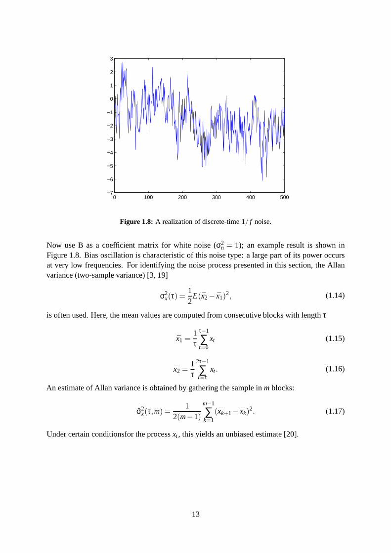
Figure 1.8: A realization of discrete-time 1/ f noise.

Now use B as a coefficient matrix for white noise (σ2n = 1); an example result is shown in

Figure 1.8. Bias oscillation is characteristic of this noise type: a large part of its power occursat very low frequencies. For identifying the noise process presented in this section, the Allanvariance (two-sample variance) [3, 19]

σ2x(τ) =

12

E(x2− x1)2, (1.14)

is often used. Here, the mean values are computed from consecutive blocks with lengthτ

x1 =1τ

τ−1

∑t=0

xt (1.15)

x2 =1τ

2τ−1

∑t=τ

xt . (1.16)

An estimate of Allan variance is obtained by gathering the sample inm blocks:

σ2x(τ,m) =

12(m−1)

m−1

∑k=1

(xk+1− xk)2. (1.17)

Under certain conditionsfor the processxt , this yields an unbiased estimate [20].

13

Problems

1.1. Consider the equation

wLEL = Fc(uL

ZL×vL)+ρZLuLZL.

What kind of a matrix is Fc when modeling the Earth as a sphere with radiusR? Whatdoes the termρZL do? Hint: Consider an aircraft flying near the North pole. If they-axisof theL-frame always points towards North, what will happen to the vectorwL

EL?

1.2. Is it possible to compute a unique position solution given the matrix CEL and altitudehonly?

1.3. In INS applications, three gyros are enough for navigation, but more of them may be usedto account for failure situations. Suppose there are three mutually orthogonal gyroscopes,and a fourth gyro is mounted such that its axis is not parallelto any of the axes of theother gyros. Is it now possible to detect if one of the gyros isgiving grossly erroneousmeasurements? If yes, is it possible to identify (and exclude) the malfunctioning gyro?Does the situation change if there are five gyros such that no three measurement axes lieon the same plane?

1.4. Show that a bias ing (gravitation model error) causes a positive feedback to INSaltitudeerror.

1.5. Suppose that one day, a MEMS gyro with analog output meets the 1 nmph INS require-ments (Table 1.1, page 11). For digitalizing the signal, an A/D converter is needed. Esti-mate the required resolution of the converter, i.e., how many bits are required for thequantization.

1.6. Through how many integrators is the termwBIB (i.e., gyro data) fed in the INS equations?

What happens to (almost) uncorrelated noise after that manyintegrations? How aboutbias-type noise?

1.7. Computer problem:Feedback couplings in INS mechanization.

1.8. Computer problem:Initializing CLB based on Earth rotation and normal force.

14

Chapter 2

Carrier Phase Based Satellite Positioning

MARTTI K IRKKO-JAAKKOLA

While tracking a satellite signal, a GNSS receiver measuresboth the phase of the modulatedranging code and the phase of the sinusoidal carrier wave. These two, i.e.,code phaseandcarrier phase, are the basic GNSS measurements, and based on them, pseudoranges and theintegrated Doppler observable can be constructed. In this chapter, using the carrier phasemeasurements for positioning is discussed. In fact, carrier measurements were not originallydesigned to be used for positioning at all; however, in the late 1970s, Counselman et al. [7]demonstrated their potential for high positioning accuracies.

As shown in Figure 2.1, code measurements are significantly more noise than carrier measure-ments: code phase measurements typically contain decimeter-level noise whereas even low-costreceivers are capable of measuring the carrier phase at centimeter precision. However, utilizingcarrier measurements is not straightforward because they only express the phase of the wavemodulo 2π∗ – by measuring the phase, one does not know the amount of full carrier cycles whichis an integer-constrained unknown for each satellite. Therefore, the use of carrier measurementsin personal positioning is usually limited to estimating the change in the distance, allowing forsmoothing the noise of code measurements (carrier smoothing, see e.g. [21]). Implementingcarrier positioning with consumer equipment is nevertheless a popular research topic [1].

2.1 Doppler Effect

Navigation satellites are constantly moving kilometers per second with respect to their users;for example, the speed of GPS satellites is around 4 km/s. Furthermore, the user may moveas well. The relative motion between the satellite and the user affects the frequency at whichthe signal is observed: if the receiver is moving towards thesignal source, it encounters wave

∗Carrier phase is usually expressed in units of carrier cycles, not radians or meters

15

−428

−426

−424

[m]

−428

−426

−424

Code Carrier

phase diff.

Figure 2.1: Noise levels in code and carrier measurements. The illustrations only show the differ-ences of consecutive measurements (all scaled to units of meters) instead of the observ-ables themselves, thus canceling bias-type errors (including integer ambiguities).

fronts more frequently than when standing still; on the other hand, when moving away fromthe transmitter, wave fronts are encountered less often. Inboth cases, the receiver observes thesignal at a different frequency than the true transmit frequency. The effect of the relative motionof the source and the receiver on the received frequency is called the Doppler effect.

For waves propagating at the speed of light∗, the Doppler shift is modeled by

fR = fT(

1− vr ·uc

)(2.1)

where fR and fT are the received and transmitted frequencies, respectively; vr is the relativevelocity between the user and the satellite;u is the unit vector pointing from the receiver antennato the satellite antenna andc is the speed of light.

The change in the frequency caused by the Doppler effect is called theDoppler shift fD:

fD = fR− fT =−vr ·uc

. (2.2)

In order to track a signal, the receiver must naturally know its Doppler-affected frequency.Therefore, the receiver also measures the Doppler shift of each satellite signal. In the followingsections we will see how we can take advantage of this.

∗This equation does not hold, e.g., for sound waves (example:the siren of an ambulance passing by), because in thatcase, the approximationv+ vs ≈ v, with v denoting the propagation speed andvs the velocity of the wave source,is invalid.

16

2.1.1 Relation between Doppler Shift and Range Rate

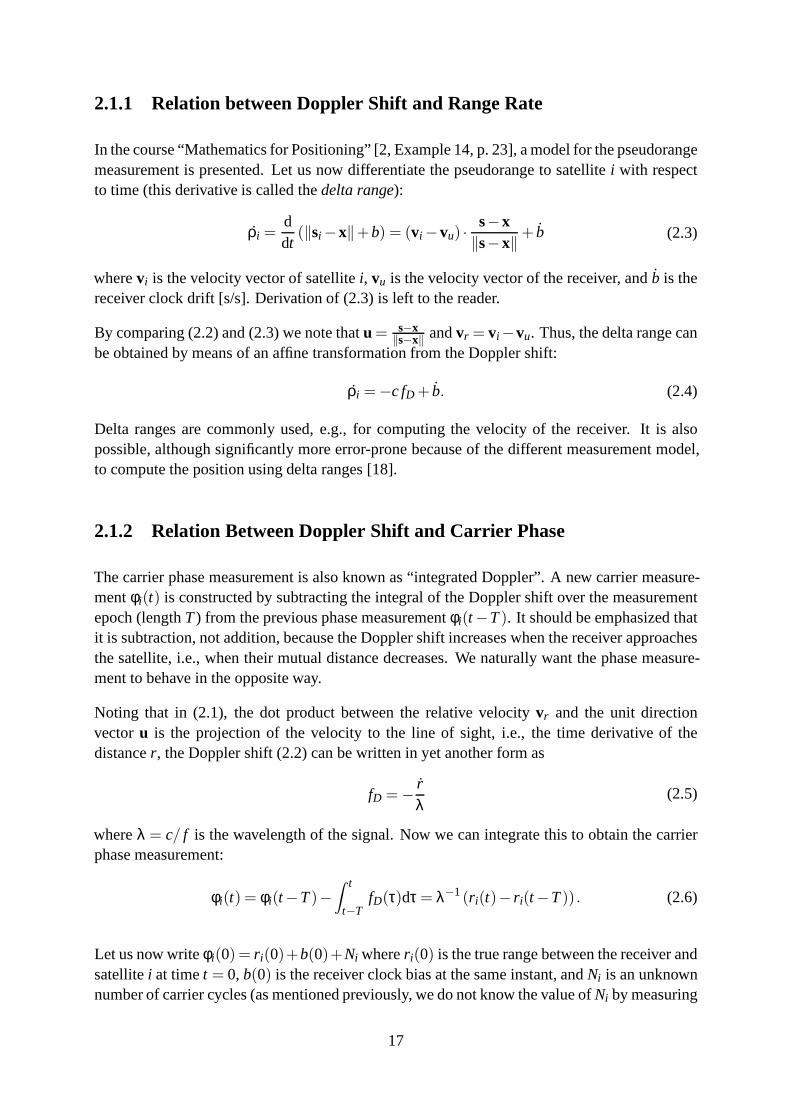
In the course “Mathematics for Positioning” [2, Example 14,p. 23], a model for the pseudorangemeasurement is presented. Let us now differentiate the pseudorange to satellitei with respectto time (this derivative is called thedelta range):

ρi =ddt

(‖si −x‖+b) = (vi −vu) ·s−x

‖s−x‖+ b (2.3)

wherevi is the velocity vector of satellitei, vu is the velocity vector of the receiver, andb is thereceiver clock drift [s/s]. Derivation of (2.3) is left to the reader.

By comparing (2.2) and (2.3) we note thatu = s−x‖s−x‖ andvr = vi −vu. Thus, the delta range can

be obtained by means of an affine transformation from the Doppler shift:

ρi =−c fD + b. (2.4)

Delta ranges are commonly used, e.g., for computing the velocity of the receiver. It is alsopossible, although significantly more error-prone becauseof the different measurement model,to compute the position using delta ranges [18].

2.1.2 Relation Between Doppler Shift and Carrier Phase

The carrier phase measurement is also known as “integrated Doppler”. A new carrier measure-mentφi(t) is constructed by subtracting the integral of the Doppler shift over the measurementepoch (lengthT) from the previous phase measurementφi(t−T). It should be emphasized thatit is subtraction, not addition, because the Doppler shift increases when the receiver approachesthe satellite, i.e., when their mutual distance decreases.We naturally want the phase measure-ment to behave in the opposite way.

Noting that in (2.1), the dot product between the relative velocity vr and the unit directionvectoru is the projection of the velocity to the line of sight, i.e., the time derivative of thedistancer, the Doppler shift (2.2) can be written in yet another form as

fD =− rλ

(2.5)

whereλ = c/ f is the wavelength of the signal. Now we can integrate this to obtain the carrierphase measurement:

φi(t) = φi(t−T)−∫ t

t−TfD(τ)dτ = λ−1(r i(t)− r i(t−T)) . (2.6)

Let us now writeφi(0) = r i(0)+b(0)+Ni wherer i(0) is the true range between the receiver andsatellitei at timet = 0, b(0) is the receiver clock bias at the same instant, andNi is an unknownnumber of carrier cycles (as mentioned previously, we do notknow the value ofNi by measuring

17

the phase) called theinteger ambiguity. Now, by introducing the satellite clock biasbi(t) and themeasurement error termεi(t) (including, e.g., satellite ephemeris errors, multipath propagationand receiver noise), the carrier phase measurement can be modeled as

φi(t) =r i(t)

λ+b(t)−bi(t)+Ni + εi(t). (2.7)

This quantity is in units of carrier cycles. In reality, error sources analogous to pseudorangeerrors, e.g., atmospheric errors, should be introduced in the model, but they have been omittedfor simplicity.

Particularly note that the integer ambiguityNi does not depend on the timet: it is determined inthe signal acquisition phase and remains constant as long assatellitei is tracked continuously.In practice, especially with low-cost equipment, the integer ambiguityNi can sometimes changedue to a short signal outage. This situation is called acycle slip, and detecting them (possiblyalso correcting for them) is crucial in precise positioningbecause each slipped cycle corre-sponds to a range error of around 20 cm. Cycle slips can be detected, e.g., from the differencesof consecutive carrier measurements using RAIM methodology (p. 37), see e.g. [14].

2.2 Differential Positioning

As stated before, the measurement model (2.7) is not realistic as it lacks some significant errorsources. When positioning in postprocessing mode where theresults are allowed to have alatency of a couple of weeks, one can use precise ephemeris and atmosphere data provided by,e.g., the International GPS Service (IGS) [9] to correct forthese biases. In real-time applica-tions, however, this is not feasible.

Another way of mitigating the errors is to take advantage of their spatial and temporal corre-lations: for instance, errors caused by atmospheric effects are practically equal for receiverslocated close to each other. This is the key idea indifferential positioningwhere areferencereceiverlocated “sufficiently close”∗

At its simplest form, differential positioning can function as follows. A reference receiver whoseexact location is known estimates how much error is includedin its measurements to move theposition estimate out of the true position. Then, this estimate of the total error, known as thedifferential correction, is broadcast to the users via, e.g., a radio link. In the absence of SelectiveAvailability (SA), these errors do not vary rapidly in time,and therefore, the correction is validfor a longer time, i.e., a new correction is not needed to be computed and broadcast at eachmeasurement epoch. The estimate of the total error also includes the clock bias of the referencereceiver; however, this does not matter as long as the users do not use both differential-correctedand uncorrected signals at the same time: the users just solve for the sum of the clock biases oftheir own and the reference receiver, which is done in the exactly same way as solving for theuser clock bias only without differential corrections.

∗“Sufficiently close” is defined totally by the situation: Forinstance, for single-frequency receivers in a bad weatheris can be a couple of kilometers whereas for dual-frequency receivers in a cloudless weather, even a hundredkilometers may be ok [21].

18

si

BaselineReference User

Figure 2.2: Single difference to satellitei.

If multiple reference receivers are available, total errorestimates are not that useful becauseit would be better if each reference would estimate the contributions of each error sourceseparately. This is how many GPS augmentations, such as the Wide Area AugmentationSystem (WAAS) in the U.S., work. A similar system, the European Geostationary Naviga-tion Overlay System (EGNOS) is available in Europe (officially since October 2009). As thename suggests, these systems use geostationary satellitesfor broadcasting correction data to alarger area. Unfortunately, geostationary satellites arebarely visible at near-polar latitudes (e.g.,in Finland) because their orbits are located directly abovethe Equator.

2.2.1 Relative Positioning

In applications where it is sufficient to only know the distance vector between two receivers,usually called thebaseline, measurements made by different receivers can be directly subtractedfrom each other without constructing separate error estimates. In this case, however, absoluteposition information is lost. If the location of one of the receivers—we will call this the refer-ence receiver—is known, we can solve for the absolute position of the other receiver (whichwe call the user, although in literature it is commonly referred to as the rover receiver) at theaccuracy of the reference location or the baseline, depending on which one is less accurate.

Using carrier measurements benefits relative positioning significantly. Since bias-type errorscan be mitigated by the differential method, measurement noise becomes a major error sourcewhen using code measurements. Carrier measurements, however, are a few orders more precise.The integer ambiguitiesNi , however, are problematic. If they can be solved for, the baseline canbe estimated possibly at a millimeter-level precision.

2.2.2 Single Difference Between Receivers

If measurements according to model (2.7) are available fromthe user and a reference receiverr“sufficiently close” to the user, as depicted in Figure 2.2, we can construct the difference of the

19

si sj

BaselineReference User

Figure 2.3: Double difference to satellitesi and j.

measurements made by these receivers to satellitei, called thesingle difference

∆rφi(t) = ∆r r i(t)λ

+∆rb(t)+∆rNi +∆rεi (2.8)

where the operator∆r denotes single differencing with receiverr. The satellite clock biasbi(t) isequal to both receivers and hence is canceled out from (2.8).Furthermore, atmospheric effectsare almost common because of the proximity assumption, and thus their effect is mitigated andthey are omitted from the model.

In contrast, the receiver clock biases, integer ambiguities, measurement noise and multipath arenot correlated between receivers and hence are not cancelled but redefined. Fortunately, evenwhen differenced, these treated analogously to those in theoriginal models, and the integerambiguities preserve their integer nature. Random measurement noise, however, is actuallyamplified: its standard deviation is increased

√2-fold, i.e.,

var∆rεi = 2varεi (2.9)

when the measurement noises of the receivers are assumed to be independent and identicallydistributed.

Denoting the baseline as∆rx = x−xr wherex andxr are the positions of the user and referencereceiver, respectively, and computing the first-order Taylor series of (2.8) yields

∆rφi(t)≈ λ−1 xr(t)−si(t)‖xr(t)−si(t)‖

·∆rx(t)+∆rNi +∆rb(t)+∆rεi(t) (2.10)

when the position of satellitei is denoted by the vectorsi . Deriving this equation is left to thereader.

20

2.2.3 Double Difference

Two single differences corresponding to different satellites can be used to construct adoubledifference∗ (Figure 2.3):

∆rφi j (t) = ∆rφi(t)−∆rφ j(t)

≈ λ−1(

xr(t)−si(t)‖xr(t)−si(t)‖

− xr(t)−sj(t)

‖xr(t)−sj(t)‖

)·∆rx(t)+∆rNi j +∆rεi j (t).

(2.11)

Differencing measurements cancels receiver-dependent biases, the most important of whichbeing the clock bias∆rb(t). The price of this operation is losing one measurement and furtheramplifying measurement noise (see problem 2.2). The integer ambiguity∆rNi j remains as aninteger, but not necessarily equal to the single-differenced ambiguity.

There are two alternative main principles for choosing the satellite pairs to be differenced. In thefixed referencemethod, one satellite is chosen as thereference!satelliteand is subtracted fromthe others. Usually, the satellite at the highest elevationangle is chosen as the reference becauseits signals propagate the shortest distance through the atmosphere and are thus probably leastaffected by atmospheric errors. Another possibility issequential differencingwhere the firstdouble difference is computed between satellites 1 and 2, the next between satellites 2 and 3,etc. In both ways,k single differences yieldk− 1 nonredundant double differences. Fixedreference is the more common way, but its drawback is that losing the reference satellite signalcauses losing all resolved integer ambiguities, as opposedto the sequential differencing wherelosing one signal causes the loss of at most two ambiguities.

2.3 Real-Time Kinematics

Real-Time Kinematic (RTK) positioning is based on the mixedinteger programming modelobtained by omitting the noise term from the double difference model (2.11). Then, theunknowns to be solved for are the baseline∆rx and the double-differenced integer ambigui-ties∆rNi j . Unfortunately, the integer constraint renders the problem hard: Even linear integerprogramming is a difficult problem for which general solution algorithms are not known, letalone nonlinear cases. The most obvious solution method, i.e., finding a solution without theinteger constraint and rounding it, does not generally work.

Integer ambiguity resolution algoritms have been extensively researched and developed.Already in the 1980s, the Ambiguity Function Method (AFM) [6] was published, and in theearly 1990s, Fast Ambiguity Resolution Approach (FARA) [10] and Least-Squares AmbiguitySearch Technique (LSAST) [11] became known. The probably most popular method, i.e.,Least-Squares Ambiguity Decorrelation Adjustment (LAMBDA) [26], was developed in themid-1990s in the Netherlands, and is briefly presented in Section 2.3.2.

∗In literature, differencing between satellites is sometimes denoted by the operator∇, and thus double differencingis denoted by the operator pair∇∆.

21

Although rounding does not usually yield a good solution estimate, the first step in RTK posi-tioning is usually constructing the nonconstrainedfloat solution, which can be done by means offiltering (in the dynamics model, the ambiguities are assumed to remain constant, but cycle slipsmust be excluded). Integer programming methods are usuallybased on exhaustive searching,and the search space is chosen to lie around the float estimate. Unfortunately, the volume of thesearch space increases rapidly: with 7 double differences available and a tolerance of±5 cycles(approximately±1 m), the search space will contain 117 candidate vectors, and searchingthrough them is obviously computationally burdensome. Moreover, when computing the floatsolution, the reliability of the solution is usually monitored, typically including cycle slip detec-tion (and usually correction because the slips are known to be multiples of the wavelength).

If the integer ambiguity resolution succeeds, the final estimate called thefixed solutioncanbe computed. To do this, the resolved ambiguities are subtracted from the respective doubledifferences, allowing for accurate estimation of the baseline.

2.3.1 Advantages of Multifrequency Receivers

In absolute pseudorange positioning, multifrequency receivers mostly serve for estimating theionospheric delay as ionosphere is dispersive and affects different frequencies at differentpowers. In RTK, however, the ionospheric error is not as significant, particularly at short base-lines, and at longer baselines, it can be estimated by means of filtering (where dual-frequencymeasurements naturally are helpful).

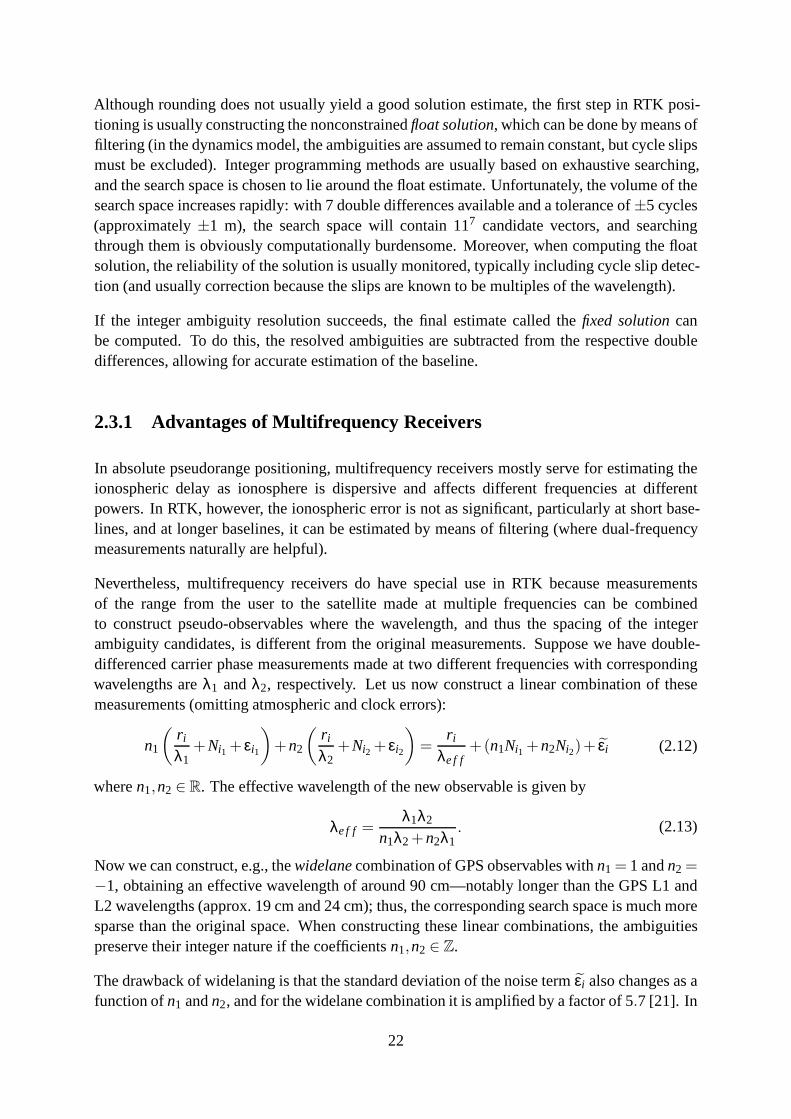
Nevertheless, multifrequency receivers do have special use in RTK because measurementsof the range from the user to the satellite made at multiple frequencies can be combinedto construct pseudo-observables where the wavelength, andthus the spacing of the integerambiguity candidates, is different from the original measurements. Suppose we have double-differenced carrier phase measurements made at two different frequencies with correspondingwavelengths areλ1 andλ2, respectively. Let us now construct a linear combination ofthesemeasurements (omitting atmospheric and clock errors):

n1

(r i

λ1+Ni1 + εi1

)+n2

(r i

λ2+Ni2 + εi2

)=

r i

λe f f+(n1Ni1 +n2Ni2)+ εi (2.12)

wheren1,n2 ∈ R. The effective wavelength of the new observable is given by

λe f f =λ1λ2

n1λ2+n2λ1. (2.13)

Now we can construct, e.g., thewidelanecombination of GPS observables withn1 = 1 andn2 =

−1, obtaining an effective wavelength of around 90 cm—notably longer than the GPS L1 andL2 wavelengths (approx. 19 cm and 24 cm); thus, the corresponding search space is much moresparse than the original space. When constructing these linear combinations, the ambiguitiespreserve their integer nature if the coefficientsn1,n2 ∈ Z.

The drawback of widelaning is that the standard deviation ofthe noise termεi also changes as afunction ofn1 andn2, and for the widelane combination it is amplified by a factor of 5.7 [21]. In

22

contrast, for example, thenarrowlanecombination (n1 = n2 = 1) has an effective wavelength ofabout 11 cm but a lower noise variance than in the original observables. Thus, the narrowlanecombination allows for more precise positioning than the original measurements, but resolvingthe integer ambiguities is more difficult. It is also possible to totally eliminate the ionosphericadvance by choosing the coefficientsn1 andn2 suitably (see problem 2.4).

2.3.2 LAMBDA method

The LAMBDA method is based on the idea that the rounding approach would work if theinteger ambiguities were not so highly correlated∗. The input of LAMBDA consists of a floatestimate vector of the double-differenced ambiguitiesN and its covariance matrix P, both ofwhich are obtained, e.g., by means of filtering. In the heart of the method is a linear transforma-tion Z that decorrelates the ambiguities as well as possible, i.e., the covariance matrix ZPZT ofthe transformed ambiguities ZN is almost diagonal. Then, the search space can be drasticallyshrunk, and, in principle, if the ambiguities could be totally decorrelated, the optimum would beobtained by rounding. The objective function of the optimization is chosen to be the differenceof the float and integer estimates weighted by the inverse of the covariance P (Integer LeastSquares; vectora denotes the integer estimate)

‖a− N‖P−1 =(

a− N)T

P−1(

a− N). (2.14)

The LAMBDA method consists of multiple steps, and its progress is outlined in Algorithm 1.

Algorithm 1 Outline of the LAMBDA method.

Precondition: N ∈ Rn is a real-valued estimate of the integer ambiguities and P= covN.

1. Compute the modified Cholesky decomposition P= LDLT .

2. Construct the LAMBDA transformation Z based on the matrices L and D.

3. Find the two best vectorsa1 anda2 according to argmina∈Zn‖a−ZN‖(ZPZT)−1.

4. Return Z−1a1 and Z−1a2.

Definition 1. An invertible matrixZ ∈ Zn×n is a LAMBDA transformation ifZ−1 ∈ Z

n×n.

If Z is a LAMBDA transformation, then in the image Z(S) of the setS⊆Rn×n, all integer vectors

of S are integer vectors, and conversely, the inverse images of all integer vectors of Z(S) areinteger vectors inS. This means that the integer ambiguities can be transformedto a decorrelatedspace using Z: in the decorrelated space the optimum is easier to find, and one can be sure thatthe obtained candidate also maps to an integer vector of the original space.

∗Double differences are highly correlated because of the waythey are constructed.

23

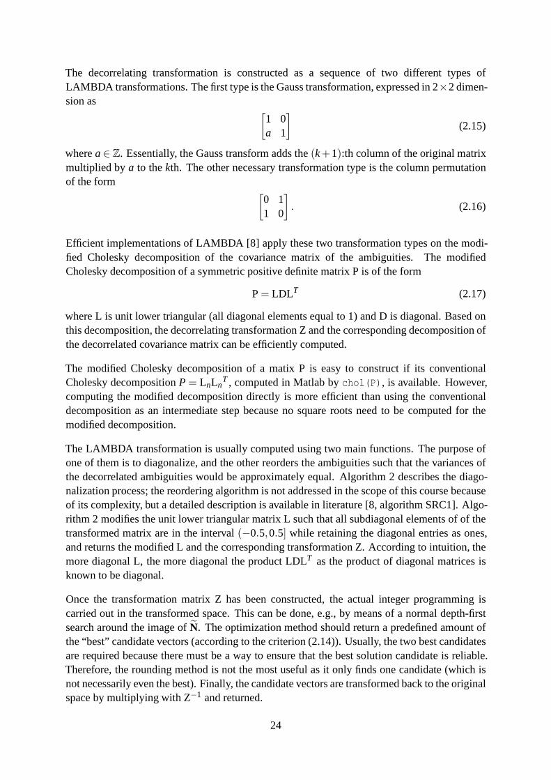
The decorrelating transformation is constructed as a sequence of two different types ofLAMBDA transformations. The first type is the Gauss transformation, expressed in 2×2 dimen-sion as

[1 0a 1

](2.15)

wherea∈ Z. Essentially, the Gauss transform adds the(k+1):th column of the original matrixmultiplied bya to thekth. The other necessary transformation type is the column permutationof the form

[0 11 0

]. (2.16)

Efficient implementations of LAMBDA [8] apply these two transformation types on the modi-fied Cholesky decomposition of the covariance matrix of the ambiguities. The modifiedCholesky decomposition of a symmetric positive definite matrix P is of the form

P= LDLT (2.17)

where L is unit lower triangular (all diagonal elements equal to 1) and D is diagonal. Based onthis decomposition, the decorrelating transformation Z and the corresponding decomposition ofthe decorrelated covariance matrix can be efficiently computed.

The modified Cholesky decomposition of a matix P is easy to construct if its conventionalCholesky decompositionP= LnLn

T , computed in Matlab bychol(P), is available. However,computing the modified decomposition directly is more efficient than using the conventionaldecomposition as an intermediate step because no square roots need to be computed for themodified decomposition.

The LAMBDA transformation is usually computed using two main functions. The purpose ofone of them is to diagonalize, and the other reorders the ambiguities such that the variances ofthe decorrelated ambiguities would be approximately equal. Algorithm 2 describes the diago-nalization process; the reordering algorithm is not addressed in the scope of this course becauseof its complexity, but a detailed description is available in literature [8, algorithm SRC1]. Algo-rithm 2 modifies the unit lower triangular matrix L such that all subdiagonal elements of of thetransformed matrix are in the interval(−0.5,0.5] while retaining the diagonal entries as ones,and returns the modified L and the corresponding transformation Z. According to intuition, themore diagonal L, the more diagonal the product LDLT as the product of diagonal matrices isknown to be diagonal.

Once the transformation matrix Z has been constructed, the actual integer programming iscarried out in the transformed space. This can be done, e.g.,by means of a normal depth-firstsearch around the image ofN. The optimization method should return a predefined amount ofthe “best” candidate vectors (according to the criterion (2.14)). Usually, the two best candidatesare required because there must be a way to ensure that the best solution candidate is reliable.Therefore, the rounding method is not the most useful as it only finds one candidate (which isnot necessarily even the best). Finally, the candidate vectors are transformed back to the originalspace by multiplying with Z−1 and returned.

24

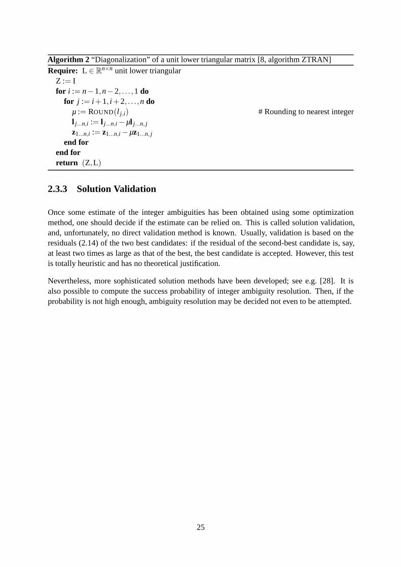
Algorithm 2 “Diagonalization” of a unit lower triangular matrix [8, algorithm ZTRAN]Require: L ∈ R

n×n unit lower triangularZ := Ifor i := n−1,n−2, . . . ,1 do

for j := i +1, i +2, . . . ,n doµ := ROUND(l j ,i) # Rounding to nearest integerl j ...n,i := l j ...n,i −µl j ...n, j

z1...n,i := z1...n,i −µz1...n, j

end forend forreturn (Z,L)

2.3.3 Solution Validation

Once some estimate of the integer ambiguities has been obtained using some optimizationmethod, one should decide if the estimate can be relied on. This is called solution validation,and, unfortunately, no direct validation method is known. Usually, validation is based on theresiduals (2.14) of the two best candidates: if the residualof the second-best candidate is, say,at least two times as large as that of the best, the best candidate is accepted. However, this testis totally heuristic and has no theoretical justification.

Nevertheless, more sophisticated solution methods have been developed; see e.g. [28]. It isalso possible to compute the success probability of integerambiguity resolution. Then, if theprobability is not high enough, ambiguity resolution may bedecided not even to be attempted.

25

Problems

2.1. Show that Equation (2.3) holds.

2.2. Show that the standard deviation of the noise in double-differenced measurements is twotimes as large as that of the original undifferenced measurements (cf. (2.9) for singledifferences), if all the original measurements are independent and identically distributed.Assume a Gaussian distribution for noise. Hint: [2, Theorem4, p. 10]

2.3. Derive Equation (2.10). Assume that the unit vector from the user location to satelliteiis equal to that from the reference location to the same satellite (as the baseline∆rx(t) isorders of magnitude shorter than the distance to the satellite).

2.4. According to the Appleton–Hartree model, the ionospheric advance expressed in units ofcarrier cycles is directly proportional to the wavelength.It is known that for the GPS L1and L2 frequencies,fL1

fL2= 77

60. Construct a linear combination of measurements made atthese frequencies such that the ionosphere term is canceledwhile preserving the ambigu-ities as integers. What is the effective wavelength of the combination?

2.5. Show that a matrix Z∈ Zn×n is a LAMBDA transformation if and only if detZ= ± 1.

Hint: Cramer’s rule.

2.6. Prove that the weighted norm (2.14) computed in the original space is equal to thatcomputed in the transformed space if the weighting is done using the covariance matrixof the respective space, i.e.,

‖a− N‖P−1 = ‖Za−ZN‖(ZPZT)−1.

2.7. Computer problem:Write a Matlab function that computes the modified Cholesky decom-position (2.17) of a symmetric positive matrix. You may callthe functionchol.

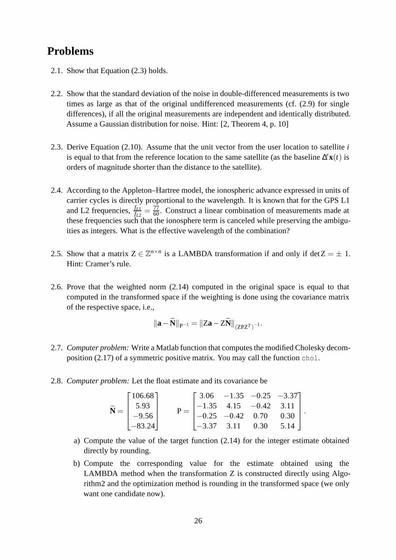
2.8. Computer problem:Let the float estimate and its covariance be

N =

106.685.93−9.56−83.24

P=

3.06 −1.35 −0.25 −3.37−1.35 4.15 −0.42 3.11−0.25 −0.42 0.70 0.30−3.37 3.11 0.30 5.14

.

a) Compute the value of the target function (2.14) for the integer estimate obtaineddirectly by rounding.

b) Compute the corresponding value for the estimate obtained using theLAMBDA method when the transformation Z is constructed directly using Algo-rithm2 and the optimization method is rounding in the transformed space (we onlywant one candidate now).

26

Chapter 3

Integrity and Reliability

HELENA LEPPÄKOSKI

From a user’s point of view, positioning cannot be considered reliable if it possible that, becauseof a system or device failure, positioning either cannot be carried out at all or yields significantlyerroneous results despite successful execution of the algorithms. This chapter presents methodsused in satellite positioning for detecting gross positionerrors and excluding erroneous measure-ments from position computations.

Reliability is related to many criteria used to describe positioning performance; these areaddressed below. Then, basics of statistical inference andhypothesis testing are reviewed.Finally, fault detection and exclusion methods for static positioning methods based on theseconcepts are presented.

3.1 Positioning Performance Metrics

In this section, positioning performance is considered in the context of satellite positioning.Some of the methods are, however, applicable on other positioning methods as well. The topicis covered in more detail in [25].

3.1.1 Accuracy

Positioning accuracy describes how close to the true position the estimates computed from themeasurements are located: the closer to the true position the estimates lie, the more accurate theyare. Accuracy is often estimated using the root mean square error (RMSE). Another commonway of quantifying accuracy is to present the statistical distribution of positioning errors, whichcan be done by means of a probability density function or a cumulative density function. A

27

simplification of these is the circular error probable (CERP) which describes the radius of thecircle centered at the true location containing a certain percentage of the (horizontal) positionestimates; for example, 95 % CERP 56 m means that at least 95 % of position estimates have atmost 56 meters of horizontal position error. The three-dimensional equivalent of CERP is thespherical error probable (SERP) where the radius of a sphereis given instead of the radius of acircle∗

Besides measurement signal quality, positioning accuracydepends on how possible measure-ment errors affect the error in the position estimate. This is determined by the satellite geometryand is quantified by the dilution of precision (DOP).

3.1.2 Integrity

The integrity of a positioning system refers to its ability of giving timely warnings when thesystem should not be used for positioning. The purpose of integrity information is to warn theuser about situations where the system outputs a positioning signal that is ostensibly normal butactually so faulty that using it corrupts the resulting position estimate significantly.

GPS satellites do broadcast integrity information to the users, but unfortunately, this informationis only available after a delay: The terrestrial control segment must first detect and identify thesatellite signal error and upload the information to the satellites for broadcasting to users. Usingthe faulty signal during this delay may have disastrous results in, e.g., aviation applications. Acritical situation may occur in terrestrial vehicle positioning as well if, e.g., an ambulance isnavigating to its destination using GPS but loses its way after using a contaminated satellitesignal, arriving at the destination too late. A similar situation occurs if the source of an emer-gency call is located using GPS, and the position is computedusing a defective satellite.

Because of the inherent latency of GPS integrity information, methods of investigating theintegrity of the signals inside the receiver have been developed. These methods are calledReceiver Autonomous Integrity Monitoring (RAIM) and are based on evaluating the consistencyof the positioning signals. RAIM can be used if redundant measurements are available, i.e., ifthe system of positioning equations is overdetermined. A lack of signal consistency can be dueto an error in a signal or in the measurement model.

Originally, RAIM was developed for civil aviation purposes. The idea was to eliminate grossmeasurement errors caused by, e.g., a satellite clock failure, and measurement model errorscaused by inaccurate knowledge of the position of a satellite (ephemeris error). Thus, thepurpose of RAIM was to detect system errors caused by the space or control segment. Sucherrors are rare: their frequency is estimated to be one errorper 18 to 24 months. Because of this,a fundamental assumption in many RAIM schemes is that no morethan one error may occur ata time.

In practice, however, the positioning signal may be corruptbecause of other reasons thanthose caused by the space and control segments. Signal reflections and multipath can cause

∗In literature, CERP and SERP are sometimes abbreviated CEP and SEP, respectively.

28

measurement errors significantly larger than normal measurement noise. With high sensi-tivity GPS (HSGPS) equipment, highly attenuated signals can be tracked at the cost of a strongamplification of noise. In the case of a poor signal-to-noiseratio, it is also possible that thereceiver locks itself to the wrong satellite, causing the possibly correct signal to be associatedwith a wrong equation, yielding in a result similar to the case of a gross ephemeris error.

This kind of errors are typical in personal positioning. Since they affect the positioning estimatein the same way as space or control segment errors do, they canbe detected and excluded usingthe same methodology as in conventional RAIM. Designing RAIM algorithms for personal posi-tioning has some additional challenges: these errors occurconsiderably more often than spaceor control segment errors, and thus, it is more likely that multiple errors occur simultaneously.

In addition to in-receiver integrity checking, external GPS monitoring station networks areavailable. These networks also broadcast information on GPS integrity, but unfortunately, thisinformation comes with a latency similar to that of the GPS navigation message. Moreover,monitoring networks cannot detect errors caused by the surroundings of the user.

3.1.3 Reliability

In general, reliability can be defined in many ways:

• Applicability of a device or system to its purpose as a function of time

• The ability of a device or system to perform the required operation under given conditionsis maintained during a given period of time

• Probability that an operational unit carries out the required operation for a given periodof time under given conditions

• A device or system meets its performance specifications

• Robustness of a device or system

In the context of satellite navigation, reliability may refer to two things: the reliability of oper-ation of the system or the statistical reliability of the positioning results. In the former case,reliability is associated with the reliability of operation of devices and components, i.e., theprobability of their correct operation, where reliabilityis quantified using, e.g., the failure prob-abilities of the components as a function of time. In contrast, statistical reliability refers to theconsistency of the measurement sequence. In satellite positioning, measurements made simul-taneously from multiple sources are available. This allowsfor examining their mutual consis-tency if the positioning problem is overdetermined, i.e., if more measurements than unknownsare available. In the context of this course, positioning reliability is considered from the pointof view of the statistical reliability of the positioning results.

In the analysis of geodetic measurement networks, reliability refers to the capability of theestimation to detect gross errors [15, 16]. This definition is analogous to the integrity monitoredby RAIM algorithms. Such a definition of reliability is applicable to analyzing the performanceof personal positioning [17].

29

The geometry of the positioning problem affects not only theaccuracy of positioning but alsothe efficiency of reliability and integrity monitoring based on consistency tests. The traditionalDOP value used for estimating positioning accuracy is not inall cases sufficient for describingthe applicability of the problem to consistency evaluation..

3.1.4 Availability

The availability of positioning is affected by many factors. In satellite positioning, the firstrequirement for availability is that the receiver must be able to receive and track a sufficientnumber of satellite signals. This does not only depend on thesatellite constellation but onthe surroundings as well—the weak satellite signals cannotpenetrate thick concrete structures.Although positioning availability may be excellent on the roof of a skyscraper, it may be poorinside the building, on the street level, in tunnels, or in underground facilities.

When assessing positioning availability, there may be additional requirements on positioningquality (i.e., accuracy and reliability) which usually decrease the quantity describing availability(probability or time percentage of availability). For instance, we may need to estimate posi-tioning availability when it is required that all satellites used for positioning must be at anelevation of at least 5◦ and they must constitute a geometry with PDOP no larger than 6.

It is also possible to possible to consider the availabilityof reliability or integrity informationseparately—to get this kind of information, more satellites are needed than for positioning only,and additional constraints are imposed on the geometry. If aposition solution is rejected becauseit is suspected to be erroneous based on integrity or reliability evaluations and there is no possi-bility to exclude the error, or if sufficient reliability is not attained because of a deficient numberof satellites or a bad geometry, the availability of positioning decreases. On the other hand, ifintegrity and reliability evaluations are omitted and all computed position solutions are accepted,the mean positioning accuracy is usually degraded, particularly in personal positioning.

3.2 Statistical Inference and Hypothesis Testing

This chapter uses the frequentistic interpretation of probability as opposed to the Bayesianinterpretation [2, p. 34].

Many algorithms for positioning integrity and reliabilitymonitoring are based on statisticalinference and hypothesis testing. The methods presented inthis chapter are reviewed in moredetail in [12, 15, 16, 17, 30]. The purpose of statistical inference is to find out the state of affairsbased on evidence. A typical question would be, e.g., “Is this industrial process producing lower-quality products than before, or can the bad quality of this sample be only a coincidence?”.When considering a set of measurements, we often deal with the question if an anomalousmeasurement is erroneous or can the observed anomaly be a coincidence, given the normalvariance of the observable.

30

For statistical inference, the question is formulated as a hypothesis, i.e., as an assumption onthe state of affairs. These assumptions (which can be eithertrue or false) are called statisticalhypotheses. Usually, a hypothesis deals with one parameterof the probability distribution ofthe phenomenon in question.

The purpose of hypothesis testing is not to prove the hypothesis to be true or false. Instead,the goal is to show that the hypothesis is not plausible because it leads to a negligible proba-bility, i.e., the observations differ significantly from measurements that would be likely if thehypothesis was true.

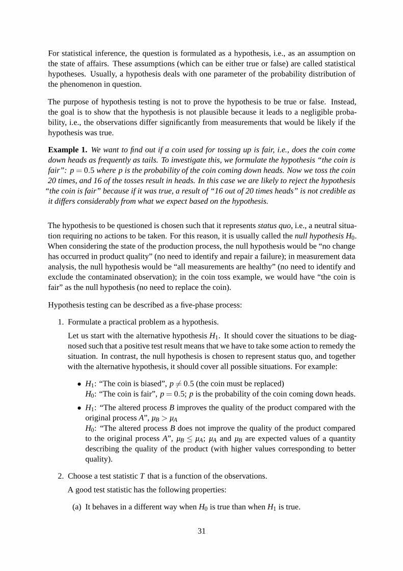
Example 1. We want to find out if a coin used for tossing up is fair, i.e., does the coin comedown heads as frequently as tails. To investigate this, we formulate the hypothesis “the coin isfair”: p = 0.5 where p is the probability of the coin coming down heads. Now we toss the coin20 times, and 16 of the tosses result in heads. In this case we are likely to reject the hypothesis

“the coin is fair” because if it was true, a result of “16 out of20 times heads” is not credible asit differs considerably from what we expect based on the hypothesis.

The hypothesis to be questioned is chosen such that it representsstatus quo, i.e., a neutral situa-tion requiring no actions to be taken. For this reason, it is usually called thenull hypothesis H0.When considering the state of the production process, the null hypothesis would be “no changehas occurred in product quality” (no need to identify and repair a failure); in measurement dataanalysis, the null hypothesis would be “all measurements are healthy” (no need to identify andexclude the contaminated observation); in the coin toss example, we would have “the coin isfair” as the null hypothesis (no need to replace the coin).

Hypothesis testing can be described as a five-phase process:

1. Formulate a practical problem as a hypothesis.

Let us start with the alternative hypothesisH1. It should cover the situations to be diag-nosed such that a positive test result means that we have to take some action to remedy thesituation. In contrast, the null hypothesis is chosen to represent status quo, and togetherwith the alternative hypothesis, it should cover all possible situations. For example:

• H1: “The coin is biased”,p 6= 0.5 (the coin must be replaced)H0: “The coin is fair”, p= 0.5; p is the probability of the coin coming down heads.

• H1: “The altered processB improves the quality of the product compared with theoriginal processA”, µB > µA

H0: “The altered processB does not improve the quality of the product comparedto the original processA”, µB ≤ µA; µA andµB are expected values of a quantitydescribing the quality of the product (with higher values corresponding to betterquality).

2. Choose a test statisticT that is a function of the observations.

A good test statistic has the following properties:

(a) It behaves in a different way whenH0 is true than whenH1 is true.

31

(b) Its probability distribution can be computed assumingH0 is true.

3. Choose the critical region.

If the value of the test statisticT lies in the critical region,H0 is rejected in favor ofH1;otherwise,H0 is not rejected. Note that no decision of acceptingH0 is made—if there isno evidence supportingH1, we only decide not to rejectH0.

When choosing the critical region, the task is to decide which values of the test statisticstrongly imply thatH1 holds. For example, the following serve as critical regions:

Right-sided H1 : T > Tcr. If the test statistic exceeds the (right-side) critical value,H0 isrejected.

Left-sided H1 : T < Tcr. If the test statistic is smaller than the (left-side) critical value,H0 is rejected.

Two-sided H1 : T < Tcr1 tai T > Tcr2. If the test statistic is either greater than the right-side critical value or smaller than the left-side critical value,H0 is rejected.

4. Decide the size of the critical region.

The starting point of statistical inference is that the decision made on rejecting or notrejectingH0 may be correct or wrong. The inference may lead to a situationwhereH0 isrejected although in reality it is true; this is called atype I error. It may also happen thatH0 is not rejected even though it actually is false; such a situation is called atype II error.

When determining the size of the critical region, it must be decided how big a risk ofmaking a wrong decision is acceptable. The probability of a type I error is called thesignificance level(or risk level) of the test and is denoted byα. Frequently used significantlevels include 5 %, 1 %, and 0.1 %. Our confidence that the decision of not rejecting thenull hypothesis is correct is reflected by theconfidence level1−α which corresponds tothe probability of the correct decision “H0 is not rejected whenH0 holds”.

The probability of a type II error is denoted byβ. Thepower of test1−β is the probabilitythat a real change of the status quo situation represented byH0 is detected because of achange in the test statistic. Table 3.1 summarizes the four possible ways of making a(right or wrong) decision in hypothesis testing.

Table 3.1: Testing a null hypothesis.

Reality Decision

H0 not rejected H0 rejected

H0 true correct decision type I errorprobability 1−α probabilityα= confidence level = significance level

H0 false type II error correct decisionprobabilityβ probability 1−β

= power of test

32

5. See if the computed value ofT lies in the critical region, and if it does, in which part ofit.

If T lies in the critical region but near the boundary, we deduce that there is some evidencesuggesting thatH0 should be rejected. In contrast, ifT lies deep in the critical region (farfrom the boundary), we have strong evidence for rejectingH0.

Example 2 (α, β and the magnitude of the detectable difference, [30]). We shall illustratehypothesis testing with an example where the geometry of theproblem is quite simple comparedto typical positioning problems. Consider the weights of male students. The null hypothesis isthat in a certain university, the mean weight of male students is68 kilograms. Let us test thehypotheses H0 : µ= 68 kgand H1 : µ 6= 68 kg; here, the alternative hypothesis covers bothµ< 68 kgand µ> 68 kg.

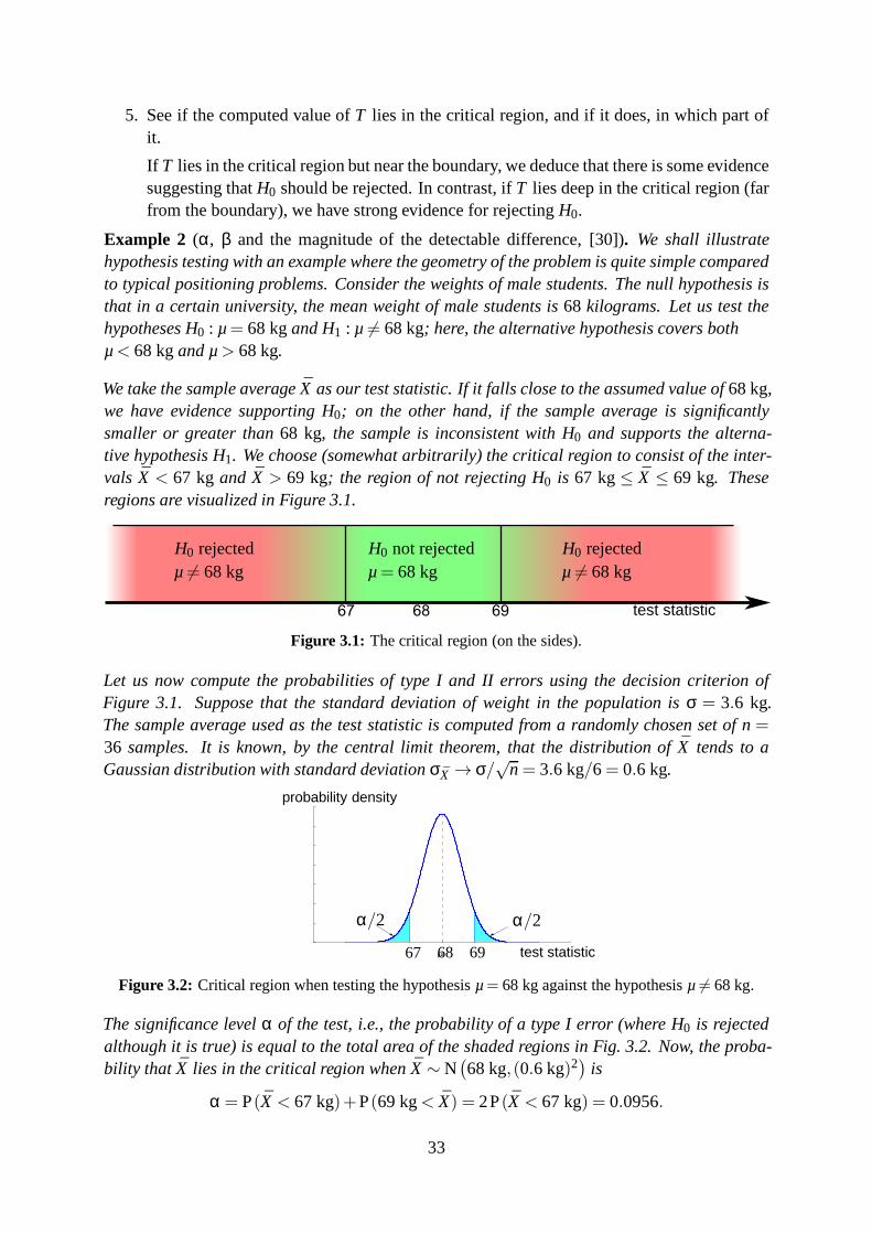
We take the sample averageX as our test statistic. If it falls close to the assumed valueof 68 kg,we have evidence supporting H0; on the other hand, if the sample average is significantlysmaller or greater than68 kg, the sample is inconsistent with H0 and supports the alterna-tive hypothesis H1. We choose (somewhat arbitrarily) the critical region to consist of the inter-vals X < 67 kg and X > 69 kg; the region of not rejecting H0 is 67 kg≤ X ≤ 69 kg. Theseregions are visualized in Figure 3.1.

H0 rejected H0 not rejected H0 rejectedµ 6= 68 kg µ= 68 kg µ 6= 68 kg

test statistic

Figure 3.1: The critical region (on the sides).

Let us now compute the probabilities of type I and II errors using the decision criterion ofFigure 3.1. Suppose that the standard deviation of weight inthe population isσ = 3.6 kg.The sample average used as the test statistic is computed from a randomly chosen set of n=36 samples. It is known, by the central limit theorem, that the distribution of X tends to aGaussian distribution with standard deviationσX → σ/

√n= 3.6 kg/6= 0.6 kg.

µ test statistic

probability density

α/2α/2

67 68 69

Figure 3.2: Critical region when testing the hypothesisµ= 68 kg against the hypothesisµ 6= 68 kg.

The significance levelα of the test, i.e., the probability of a type I error (where H0 is rejectedalthough it is true) is equal to the total area of the shaded regions in Fig. 3.2. Now, the proba-bility that X lies in the critical region whenX ∼ N

(68 kg,(0.6 kg)2

)is

α = P(X < 67 kg)+P(69 kg< X) = 2P(X < 67 kg) = 0.0956.

33

According to the result,9.6 %of all sets of36 samples would cause rejecting the hypothesisµ= 68 kgalthough the hypothesis would hold. In order to decrease theprobabilityα, either thesample size n should be increased (thus decreasing the sample variance) or the non-rejectingregion should be expanded. Suppose the sample size is increased to n= 64. Then,σX = 3.6/8= 0.45and

α = 2P(X < 67 kg) = 0.0263.

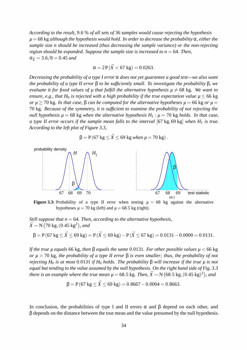
Decreasing the probability of a type I errorα does not yet guarantee a good test—we also wantthe probability of a type II errorβ to be sufficiently small. To investigate the probabilityβ, weevaluate it for fixed values of µ that fulfill the alternative hypothesis µ6= 68 kg. We want toensure, e.g., that H0 is rejected with a high probability if the true expectation value µ≤ 66 kgor µ≥ 70 kg. In that case,β can be computed for the alternative hypotheses µ= 66 kgor µ=

70 kg. Because of the symmetry, it is sufficient to examine the probability of not rejecting thenull hypothesis µ= 68 kgwhen the alternative hypothesis H1 : µ= 70 kgholds. In that case,a type II error occurs if the sample mean falls to the interval[67 kg,69 kg] when H1 is true.According to the left plot of Figure 3.3,

β = P(67 kg≤ X ≤ 69 kgwhen µ= 70 kg) .

probability densityHH 1

β

67 68 69 70

β

67 68 69 test statistic68.5

Figure 3.3: Probability of a type II error when testingµ = 68 kg against the alternativehypothesesµ= 70 kg (left) andµ= 68.5 kg (right).

Still suppose that n= 64. Then, according to the alternative hypothesis,X ∼ N

(70 kg,(0.45 kg2

), and

β = P(67 kg≤ X ≤ 69 kg) = P(X ≤ 69 kg)−P(X ≤ 67 kg) = 0.0131−0.0000= 0.0131.

If the true µ equals66 kg, thenβ equals the same0.0131. For other possible values µ< 66 kgor µ> 70 kg, the probability of a type II errorβ is even smaller; thus, the probability of notrejecting H0 is at most0.0131 if H0 holds. The probabilityβ will increase if the true µ is notequal but tending to the value assumed by the null hypothesis. On the right hand side of Fig. 3.3there is an example where the true mean µ= 68.5 kg. Then,X ∼ N

(68.5 kg,(0.45 kg)2

), and

β = P(67 kg≤ X ≤ 69 kg) = 0.8667−0.0004= 0.8663.

In conclusion, the probabilities of type I and II errorsα and β depend on each other, andβ depends on the distance between the true mean and the value presumed by the null hypothesis.

34

3.3 Residuals

In this section, the properties of residuals are reviewed. Moreover, some notation different fromwhat has previously been used in this hand-out and [2] is introduced. It is assumed that theobservables and unknowns are related by a linear measurement model of the form

y = Hx+ εεε (3.1)

where then× 1 vector y contains the measurements,εεε contains measurement errors, them× 1 vectorx is composed by the states (i.e., the parameters to be estimated), and the measure-ment matrix H describes the linear relation between the measurements and states. In the contextof positioning, the matrix H is commonly referred to as the geometry matrix. In practical posi-tioning applications, however, the underlying model is usually nonlinear; in such cases, H isobtained by linearizing the system of nonlinear measurement equations,x is the change of stateobtained in the last iteration cycle, andy is the difference between observed and computedmeasurements.

Suppose the position is resolved using the weighted least squares (WLS) method. If the weightsare chosen as the inverse of the covariance matrix of the measurements, the WLS method yieldsthe best linear unbiased estimate (BLUE). The covariance ofmeasurement errors is assumedknown:V (y) =V (εεε) = Σ with Σ > 0. Then, the WLS solution is given by

x =(HTΣ−1H

)−1HTΣ−1y = Ky. (3.2)

Furthermore, we assume that the measurement covariance matrix is diagonal, i.e., the measure-ments are mutually uncorrelated. The residualsv can be written as a function of the measure-ments:

v = Hx−y = HK y−y = (HK − I) y =−Ry (3.3)

where the matrix R is called theredundancy matrix. It is left to the reader to show that theredundancy matrix is idempotent, i.e.,R2 = R. The covariance of the residuals can be expressedusing the geometry matrix and the covariance of the measurements (see Problem 3.2):

Cv =V(v) = (HK − I)V (y)(HK − I)T = Σ−H(HTΣ−1H

)−1HT . (3.4)

Furthermore, the redundancy matrix can be expressed using the covariance matrices of theresiduals and the measurements (Problem 3.2):

R= CvΣ−1. (3.5)

3.3.1 Quadratic Form of Residuals

The quadratic form of residualsvTΣ−1v is a common test statistic in positioning reliabilityanalysis. We assume that measurement errors in (3.1) are normally distributed:εεε ∼ N(µµµ,Σ).

35

The quadratic form can be written using the measurements:

vTΣ−1v = (−Ry)T Σ−1(−Ry) = εεεTRTΣ−1Rεεε.

Let us write A= RTΣ−1R. To be able to use the result [2, Theorem 6, p. 11], we must ensurethe idempotency of the matrix AΣ. Using (3.5), we may write

A = RTΣ−1R=(CvΣ−1)T Σ−1CvΣ−1 = Σ−1CvΣ−1CvΣ−1 = Σ−1RR= Σ−1R, (3.6)

becauseΣ−1 and Cv are symmetric matrices and R is idempotent. This gives AΣ and AΣAΣ:

AΣ = Σ−1RΣAΣAΣ = Σ−1RΣΣ−1RΣ = Σ−1RRΣ = Σ−1RΣ = AΣ.

Hence, RTΣ−1RΣ is idempotent andvTΣ−1v ∼ χ2(n−m,λ) where rank(RTΣ−1R) = n−m(Problem 3.3) is the number of degrees of freedom,n is the number of measurement equations,andm is the number of states to be estimated. If measurement errors are assumed to have zeromean, i.e.,µµµ= 0, the noncentrality parameterλ equals zero and the quadratic form follows acentralχ2 distribution. On the other hand, if we assume that not all measurement errors havezero mean, i.e.,µµµ 6= 0, the noncentrality parameter becomesλ = µµµTAµµµ= µµµTRTΣ−1Rµµµ and thequadratic form is noncentrallyχ2 distributed.

Consider a caseεεε ∼ N(µµµ,Σ) where the measurementyi is biased, i.e., its error has a nonzeromean while other measurement errors have zero mean:

E(εi) =µi 6= 0

E(ε j)=µj = 0 ∀ j 6= i with j = 1. . .n.

Denote the diagonal elements ofΣ as[Σ](i,i) = σ2i . Now, the value of the noncentrality param-

eterλ can be computed based on (3.5) and (3.6) utilizing the diagonality of Σ:

λ = µµµTAµµµ= µ2i [A](i,i) = µ2

i

[Σ−1R

](i,i)

= µ2i

[Σ−1CvΣ−1]

(i,i) =µ2

i

σ4i

[Cv](i,i) .(3.7)

3.3.2 Standardized Residuals

Standardized residualswi are obtained by dividing residuals by the square roots of their respec-tive variances:

wi =vi√

[Cv](i,i)

, i = 1. . .n.(3.8)

Consider again a caseεεε ∼ N(µµµ,Σ) with yi being biased while other measurement errors havezero mean:µi 6= 0, µj = 0 ∀ j 6= i where j = 1. . .n.

36

By (3.3), the expectation value of the residual vector is

E(v j)= E

([−Ry] j

)=− [R]( j ,i)µi,

and the expectation of the standardized residuals is

E(w j

)= E

(v j /

√[Cv]( j , j)

)=−µi [R]( j ,i) /

√[Cv]( j , j)

=−µi [Cv]( j ,i)

[Σ−1]

(i,i)/√

[Cv]( j , j)

=−µi/σ2i [Cv]( j ,i) /

√[Cv]( j , j).

The expected value of the standardized residual of measurement i becomes

E(wi) =−µi/σ2i

√[Cv](i,i). (3.9)

3.4 Receiver Autonomous Integrity Monitoring

RAIM consists of two steps. First, the algorithm needs to findout if the measurements ormeasurement models are erroneous or not; this is called fault detection. In the second phase,the algorithms searches for a combination of measurement that does not contain erroneousequations. This step is carried out only if an error is detected in the first phase.

There are two approaches to carrying out the second step of RAIM. The first alternative isto identify the faulty equation and exclude it from computations; this method is called FaultDetection and Identification (FDI). The other approach is toconstruct such a combination ofthe available measurements that seems to be error-free, i.e., does not trigger a fault alarm inthe first step of RAIM; this approach is known as Fault Detection and Exclusion (FDE). Faultexclusion does not require pinpointing the faulty measurement: Suppose that measurement 3is faulty. Now, if we exclude measurements 3, 4, and 5, we haveeliminated the error but notidentified it precisely. As FDI and FDE have the same goal (i.e., excluding the faulty equation),the whole process is often referred to as FDE.

If satellite positioning is only used as a complementary means of navigation, sole fault detec-tion may be sufficient. In such a scenario, the system will useanother method of navigation,e.g., INS, if RAIM detects a fault in the satellite navigation equations. In contrast, if satellitepositioning is the only available navigation method, excluding the error is obviouly preferableto beíng totally left without a position solution.

Using RAIM methods poses a requirement of redundancy. Whiletraditional satellite positioningrequires a minimum of four measurements for a position solution, RAIM needs at least fivemeasurements for fault detection and six or more for FDE.

Many virtually different RAIM methods exist: e.g., the parity space method, range comparison,and the least squares residual method. In GPS literature, these have been shown to be mutuallyequivalent; hence, in this section we will concentrate on the approach based on least squaresresiduals.

37

3.4.1 Fault Detection

We take (3.1) as our measurement model andΣ = σ2I as the measurement covariance. Then, theweight matrix in the WLS solution (3.2) is identity, yielding K=

(HTH

)−1HT and a redundancy

matrix of R= I−H(HTH

)−1HT .

Our observable for fault detection is the sum of the squares of the residuals, commonly knownas SSE (Sum of Squares of Errors):SSE= vTv. In the case of zero-mean measurementerrors,SSE∼ χ2(n−4) wheren is the number of available measurements. However, if themeasurements are not zero-mean,SSEfollows a noncentral distribution:SSE∼ χ2(n−4,λ).

The test statistic is chosen to be

T =

√SSEn−4

=

√vTvn−4

where the purpose of taking the square root and dividing by the number of degrees of freedomis to reduce dependency on satellite geometry. As the critical value we take

Tcr =

√σ2×χ2

1−pf a(n−4)

n−4,

whereχ21−pf a

(n−4) is the inverse cumulativeχ2 density function with the probability 1− pf a

as its argument and the number of degrees of freedom in the parentheses. The probabilitypf a

is the false alarm rate. In typical RAIM implementations,pf a is given a very small value; e.g.,in civil aviation with GPS being the primary means of navigation, pf a = 0.333·10−6 [13].

3.4.2 Effect of Geometry

The effect of satellite geometry on the error detection capability of RAIM is investigated bycomparing the impacts of a measurement error on the positionestimate and on the residual. Ifan error affects the residual only slightly but has a significant effect on the position solution,RAIM cannot protect the user from large position estimate errors very well. In such cases, theuser must be at least warned—a bad geometry does not necessarily imply measurement faults,but if a fault occurs, it is unlikely to be noticed.

In the following, the concept of Approximate Radial Error Protected (ARP) is presented asan example. The purpose of ARP is to detect geometries disadvantageous for RAIM; othermethods for ensuring a geometry sufficient for RAIM have beendeveloped as well.ARPgivesa coarse approximation of the maximum position error that RAIM may fail to detect, and iscomputed by

ARP= SmaxTcr

38

whereSmax is the maximum of the slopesSi describing the relation between the test statistic anda bias in theith measurement:

Si =

√√√√([K]2(1,i)+[K]2(2,i)

)(n−4)

[R](i,i).

Here, we assume that the geometry is expressed in the ENU frame; then, the top two rows ofthe matrixK correspond to the horizontal components of the position estimate. Now, to screenout bad geometries,ARP is compared to a predefined threshold valueARPcr: if ARP< ARPcr,RAIM is considered unavailable. Otherwise, whenARP≥ ARPcr, RAIM is just unable to detectposition errors smaller than the ARP threshold.

3.4.3 Fault Identification/Exclusion

If a fault is detected andn≥ 6 measurements are available, we constructn measurement subsetssuch that one of the original satellites is missing from eachsubset. Then, the ARP value iscomputed for each subset; if all of them are acceptable, the corresponding test statistics areevaluated. If there is exactly one biased measurement present, it should be missing from one ofthe subsets, and thus, the test statistic value of that subset should be less than the critical valueas opposed to other subsets: they contain the fault and theirtest statistic values should exceedthe critical value.

If the subset testing method finds only one subset whose test statistic does not trigger a faultdetection alarm, the measurement missing from that subset is regarded as faulty and the positionsolution corresponding to that subset is accepted. In contrast, if multiple subsets have a teststatistic value less than the critical value or not all subsets pass the ARP test, the error cannotbe reliably identified. Then, the obtained position estimate cannot be improved and is flaggedas unreliable.

3.5 Reliability Testing Based on Global and Local Tests

The reliability testing method presented in this section originates from reliability analysis ofgeodetic measurement networks [16] where the concepts are somewhat different from thoseof RAIM. Nevertheless, both are based on similar principles: statistical reliability testing is usedto investigate if the measurements agree with assumptions.First, the entire set of measurementsis examined in aglobal testto detect outliers. Then, if an error was detected,local testsareconducted in order to identify the erroneous measurements.The method is theoretically basedon the case of a single outlier but has been extended to practical applications with multiplesimultaneous errors. For examples and further reading, see[17].

39

The null hypothesis is “no biased measurements”, under which all measurement errors have zeromean. The alternative hypothesis is “at least one measurement is biased”, i.e., the measurementerrors are not zero-mean:

H0 : εεε ∼ N(0,Σ)H1 : εεε ∼ N(µµµ,Σ) whereµµµ 6= 0.

3.5.1 Global Test

The purpose of the global test is to find out if the set of measurements contains faults or not.The quadratic form of the residuals serves as the test statistic:

T = vTΣ−1v.

According to Section 3.3.1,T follows a centralχ2 distribution if H0 holds, and a noncentralχ2 distribution if H1 is true. The number of degrees of freedomn−m is determined by thenumber of available measurementsn and the number of unknown statesm. In contrast, choosingthe noncentrality parameterλ is a part of designing the test.

As a random variable following a centralχ2 distribution gets smaller values than a noncentrallyχ2 distributed variable with as many of degrees of freedom, we choose a right-sided criticalregion. Thus, our hypotheses to be tested are

H0 : T ≤ Tcr

H1 : T > Tcr.

For determining the critical value, we decide the significance levelα of the test, i.e., an accept-able probability of a type I error. The critical valueTcr is chosen such thatT ∼ χ2(n− p)implies P(T > Tcr) = α, i.e.,

Tcr = χ21−α (n−m)

whereχ2p(·) denotes the inverse cumulativeχ2 density function withp as its argument and the

degrees of freedom in parentheses.

Conducting the global test does not require choosing the probability β or the noncentralityparameterλ. Nevertheless, it is good to be familiar with the dependencybetween them. Further-more, using these values, the parameters of the global test can be related to those of the localtest.

Based on Example 2 (p. 33) it was stated that the probabilities of type I and II errors are inter-dependent, and the magnitude ofβ is affected by the difference between the null hypothesisassumption and reality. This is utilized when choosing the value ofλ: first, we decide an accept-able probability of wrong decisionβ; then, we findλ such that the cumulative density functionof χ2(n−m,λ) evaluates toβ at the same value ofT as where the cumulative density functionof χ2(n−m) evaluates to 1−α, i.e.,

χ21−α (n−m) = χ2

β (n−m,λ) .

40

−5 0 5 10 15 20 250

0.05

0.1

0.15

0.2

0.25

Tkr

β

α

n − m = 3 α = 0.11 β = 0.20 λ = 6.03

test statistic

probability density

Figure 3.4: Relation between the parametersα, β, λ, andTcr.

Figure 3.4 visualizes the choice of the parameters in a case with 3 degrees of freedom. Theprobabilitiesα = 0.11 andβ = 0.20 have been chosen such that the regions corresponding tothem are clearly visible in the figure. However, in practice,these probabilities—particularlyα—are chosen to be much smaller, e.g.,α = 0.001; commonly used values ofβ are, e.g., 0.2, 0.1,and 0.05.

3.5.2 Local Test

If the global test results inT > Tcr, we deduce that at least one biased measurement ispresent. The local test attempts to identify observations that should be suspected of blun-ders. According toH0, the distribution of the measurement errorsεεε is N(0,Σ), and conse-quently, the residualsv follow a N

(0,RΣRT

)distribution. As the standardized residuals are,

according to (3.8), obtained by scaling each residual by thereciprocal of its standard deviation,we havewi ∼ N(0,1).

The hypotheses to be tested are reduced to concern the standard normal distribution by takingthe standardized residual as the test statistic. As opposedto the global test examining the entireresidual vector at once, each residual is tested separatelyin the local test. The hypothesesconcerning the residualwi are

H0 : wi ∼ N(0,1)

H1 : wi ∼ N(δ,1) whereδ 6= 0.

The corresponding regions of the test statistic are

H0,i : −wcr ≤ wi ≤ wcr

H1,i : wi <−wcr or wi > wcr.

41

Since the distribution is symmetric, we may reduce these two-sided tests to right-sided by takingthe absolute value of the standardized residual as the test statistic of the local test:

H0,i : |wi | ≤ wcr

H1,i : |wi |> wcr.

In the local test, the alternative hypothesis states that the meanδ of the distribution is nonzero,whereas in the global test, the noncentrality parameterλ is assumed to be nonzero. These param-eters are interdependent; thus, the quantitiesδ andλ associated with the alternative hypothesescan be determined using each other. As in both tests the probability β depends on the deviationof the parameter of the null hypothesis (λ = 0 andδ = 0) from reality and vice versa, it is naturalto use the same probabilityβ for bothδ andλ.

Both in the global and local test, the alternative hypothesis is based on the assumption thatmeasurement errors are normally distributed but have a nonzero mean. Suppose all measure-ment errors are normally distributed with zero mean except for the ith measurement that isbiased:E(εi) = µi . Let us now compare how the bias in measurementi affects the parameterλand the expectation value of theith standardized residualE (wi). Equations (3.7) and (3.9) showthatλ = E (wi)

2, yielding|E (wi)|=√

λ. Since we are now considering the absolute value ofwi

in the local test, we are only interested in those distributions of the alternative hypothesis wherethe mean is positive. Then,

δ = |E (wi)|=√

λ.

−6 −4 −2 0 2 4 6 80

0.05

0.1

0.15

0.2

0.25

0.3

0.35

0.4

α0/2 α

0/2

β

δ = 2.45

w = 1.61

α0 = 0.107

δ

a b

test statistic

probability density

cr

Figure 3.5: Relation between the parametersα0, β, δ, andwcr.

Two of the parametersα0, β, δ, andwcr need to be fixed for determining the rest. Figure 3.5shows the following relations:

a= n1−α0/2(0,1) = wcr

b= δ−nβ (δ,1) = n1−β (δ,1)−δ = n1−β (0,1)+δ−δδ = a+b= n1−α0/2(0,1)+n1−β (0,1)

42

wherenp(·) is the inverse cumulative normal distribution function with p as its argument andthe parameters of the distribution in parentheses.

3.5.3 Internal and External Reliability

The internal reliability of a positioning problem is quantified by the minimum detectablebias (MDB; also referred to as marginally detectable bias),i.e., the smallest measurement errorthat can be detected by means of statistical testing. In contrast,external reliabilityexpresses theeffect of the minimum detectable bias on the position estimate.

The expectance valueδ corresponds to the smallest bias in a standardized residualthat can bedetected at probability 1−β with a confidence level of 1−α. The absolute value of MDB formeasurementi is given by

mi =δ [Σ](i,i)√[Cv](i,i)

. (3.10)

External reliability describes the impact of the MDB on the position estimate. Suppose measure-menti is biased bymi and other measurements are unbiased, i.e., the measurementerror vectorequals∆yi = [0. . .0 mi 0. . .0]T . We can now compute the external reliability:

ei = K∆yi = [K](1:n,i)mi =[(

HΣ−1HT)HTΣ−1](1:n,i)mi . (3.11)

The purpose of external reliability is to describe the magnitude of the errors from which statis-tical testing can protect—errors smaller than the externalreliability are not detected. Whenconsidering a typical positioning problem with the first three components of the state vectorreferring to position coordinates, external reliability can be used for computing the radius of thesphere containing all position estimates biased by undetected measurement errors:

rPPLi =√

e2i1+e2

i2+e2

i3.

External reliability is also known as the position protection level (PPL). If the positioningcomputations have been done in the ENU frame or the external reliability ei is transformedto that frame, we may compute the horizontal protection level (HPL)

rHPLi =√

e2i1+e2

i2,

describing the radius of the circle containing all horizontal position biases caused by undetectedmeasurement errors.

The protection levelsrPPLi andrHPLi are different for each measurement; hence, a (somewhatpessimistic) estimate of the total protection level can be obtained by computing the protectionlevel for each measurement and choosing the maximum:rPPLi = maxi rPPLi , and correspond-ingly for HPL. In this context, a larger protection level means that larger errors may pass throughthe testing undetected.

43

As reliability testing fails at detecting the presence of smallest possible biases, they cannot beidentified either. On the other hand, a gross measurement error may have a significant impacton the position estimate the iterative (weighted) least squares solution method converges to. Insuch cases, the linearization point may be very far from the true location, inducing significanterrors in the geometry matrix as well. Such errors tend to increase all residuals, which usuallycan be seen in the test statistic of the global test. In contrast, pinpointing the true outlier can bedifficult because the geometry matrix used in the analysis isfaulty.

3.5.4 Fault Detection and Exclusion

In practice, the FDE process is iterative. Detecting the presence of measurement errors isattempted by means of global testing. If errors are detected, a local test is coducted for eachstandardized residualwi . As more than one error may occur at a time, multiple standardizedresiduals not passing the local test may be encountered.

A residual vi with a large absolute value may be due to an error in some othermeasure-ment thanyi . The redundancy matrix R that maps measurement errors to residuals sometimescontains offdiagonal elements satisfying

∣∣∣[R]( j ,i)

∣∣∣> [R](i,i) or∣∣∣[R](i, j)

∣∣∣> [R](i,i) .

In the first case, an error in theith observation affects the residualj more strongly than its respec-tive residual. In the second case, residuali is more affected by measurementj than its corre-sponding measurementi. Both scenarios render fault identification either hard or impossible—the possibility of such a problem may be found out beforehandby examining the elements ofthe matrix R.

Because of the reasons mentioned above, a test statistici not passing the local test should notbe regarded as a reason to label the corresponding measurement yi as faulty; instead, it onlysuggests thatyi suspicious. Then, the global test is repeated without the suspected measure-ment(s). If it still indicates the presence of errors, the testing continues. Finally, once (or if)a measurement combination that passes the global test is found, it should be tried if any ofthe excluded measurements could be included again without the global test indicating errors.This is due to the possibility that a gross outlier that has been later excluded may have stronglyaffected residuals whose corresponding measurements havebeen excluded first.

44

Problems

3.1. (a) Show that the redundancy matrix R is idempotent (i.e., R2 = R).

(b) What kind of a weight matrixΣ−1 is needed for the redundancy matrix to besymmetric?

3.2. (a) Show that for the covariance of residuals, Cv = Σ−H(HTΣ−1H

)−1HT (3.4).

(b) Show that R= CvΣ−1 (3.5).

3.3. Show that rank(RTΣ−1R) = n−m. Hint: show that

(a) x∈ N (RTΣ−1R) if and only if x∈ N (R)

(b) x∈ N (R) if and only if x∈ R (H)

(c) dim(R (H)) = m

45

Index

accelerometer, 4accuracy, 27AFM, 21Allan variance, 13availability, 30

baseline, 19, 20

carrier phase, 18carrier phase based positioning, 15CERP, 28Cholesky decomposition, 24

modified, 24clock bias, 17, 21

satellite, 18clock drift, 17confidence level, 32Coriolis force, 5critical region, 32cycle slip, 18, 22

delta range, 17difference

double, 21single, 19

differential correction, 18Doppler

effect, 16integrated, 17shift, 16

ephemeris error, 28error

ephemeris, 18, 28satellite clock, 18, 28type I, 32type II, 32

FARA, 21

FDE, 37FDI, 37fixed reference, 21fixed solution, 22float solution, 22

geometry matrix, 35gyroscope

mechanical, 5ring laser, 7tuning fork, 5

hypothesisalternative, 31null, 31statistical, 31testing, 31

inertia, 4inertial navigation, 8integer ambiguity, 18, 21integer least squares, 23integrity, 28

LAMBDA, 21, 23transformation, 23

LSAST, 21

measurementcarrier, 15

measurement errors, 9measurement model

carrier phase, 18MEMS, 6misalignment, 10

narrowlane, 23

parts per million, 10

46

power of test, 32protection level

horizontal, 43position, 43

pseudo-observable, 22

RAIM, 28, 37real-time kinematics, 21redundancy matrix, 35reference

fixed, 21receiver, 18, 19

reliability, 22, 29external, 43internal, 43

residual, 25, 35standardized, 36

rover receiver, 19RTK, 21

Sagnac effect, 6scale factor, 10sequential differencing, 21SERP, 28significance level, 32status quo, 31

type I error, 32type II error, 32

unit lower triangular matrix, 24

weighted norm, 23widelane, 22WLS, 35

47

References

Most of the references can be found either online or in the TUTlibrary. Publications of IEEEcan be found in IEEE Xplore,http://ieeexplore.ieee.org/, where the full articles areaccessible when connecting from the TUT network (or via a TUTVPN connection).

[1] A LANEN , K., WIROLA , L., KÄPPI, J., AND SYRJÄRINNE, J. Mobile RTK: Using low-cost GPS and internet-enabled wireless phones.Inside GNSS 1(2006), 32–39.

[2] A LI -LÖYTTY, S., COLLIN , J., AND SIROLA , N. Mathematics for Positioning. Lecturehand-out, TUT, Department of Mathematics, 2009.http://math.tut.fi/courses/MAT-45806/.

[3] A LLAN , D. W., ASHBY, N., AND HODGE, C. C. The science of timekeeping. Applica-tion note 1289, Hewlett Packard, 1997.http://www.allanstime.com/Publications/DWA/Science_Timekeeping/TheScienceOfTimekeeping.pdf.

[4] BAILLIE , R. Long memory processes and fractional integration in econometrics.Journalof Econometrics 73, 1 (1996), 5–59.

[5] COLLIN , J. Investigations of Self-Contained Sensors for Personal Navigation. Disser-tation, Tampere University of Technology, 2006.http://webhotel.tut.fi/library/tutdiss/pdf/collin.pdf.

[6] COUNSELMAN, C. C., AND GOUREVITCH, S. A. Miniature interferometer terminalsfor earth surveying: Ambiguity and multipath with Global Positioning System. IEEETransactions on Geoscience and Remote Sensing GE-19, 4 (1981), 244–252.

[7] COUNSELMAN, C. C., SHAPIRO, I. I., GREENSPAN, R. L., AND COX, JR., D. B.Backpack VLBI terminal with subcentimeter capability.Proc. Radio Interferometric Tech-niques for Geodesy(1979), vol. 2115, NASA Conference Publication, pp. 409–413.

[8] DE JONGE, P., AND TIBERIUS, C. The LAMBDA method for integer ambiguity estima-tion: implementation aspects.LGR Publication, Delft University of Technology, 12 (1996),61–66.

[9] DOW, J., NEILAN , R., AND GENDT, G. The International GPS Service (IGS): Cele-brating the 10th anniversary and looking to the next decade.Advances in Space Research36, 3 (2005), 320–326.

48

[10] FREI, E., AND BEUTLER, G. Rapid static positioning based on the fast ambiguity reso-lution approach FARA: Theory and first results.Manuscripta Geodaetica 15, 6 (1990),325–356.

[11] HATCH, R. Instantaneous ambiguity resolution.Proceedings of IAG International Sympo-sium No. 107 on Kinematic Systems in Geodesy, Surveying and Remote Sensing(1990),Springer Verlag, pp. 299–308.

[12] KANJI, G. K. 100 Statistical Tests. SAGE Publications Ltd, 1999.

[13] KAPLAN , E. D., Ed. Understanding GPS: principles and applications. Artech House,Norwood, 2005.

[14] K IRKKO-JAAKKOLA , M., TRAUGOTT, J., ODIJK, D., COLLIN , J., SACHS, G., AND

HOLZAPFEL, F. A RAIM approach to GNSS outlier and cycle slip detection using L1carrier phase time-differences.Proceedings of the IEEE Workshop on Signal ProcessingSystems SiPS’09(Tampere, Finland, 2009), pp. 273–278.http://ieeexplore.ieee.org/.

[15] KOCH, K.-R. Parameter Estimation and Hypothesis Testing in Linear Models, 2nd ed.Springer-Verlag Berlin Heidelberg, 1999.

[16] KUANG, S. Geodetic Network Analysis and Optimal Design: concepts andApplications.Ann Arbor Press Inc., 1996.

[17] KUUSNIEMI, H. User-Level Reliability and Quality Monitoring in Satellite-BasedPersonal Navigation. Dissertation, Tampere University of Technology, 2005.http://webhotel.tut.fi/library/tutdiss/pdf/kuusniemi.pdf.

[18] LEHTINEN, A. Doppler Positioning with GPS. M.Sc. Thesis, Tampere University of Tech-nology, 2002.http://math.tut.fi/posgroup/DopplerPositioningwithGPS.pdf.

[19] LESAGE, P., AND AUDOIN, C. Effect of dead-time on the estimation of the two-samplevariance. IEEE Transactions on Instrumentaiton and Measurement 28, 1 (1979), 6–10.http://ieeexplore.ieee.org/.

[20] MASRY, E. Flicker noise and the estimation of the allan variance.IEEE Transactions onInformation Theory 37, 4 (1991), 1173–1177.http://ieeexplore.ieee.org/.

[21] M ISRA, P., AND ENGE, P. Global Positioning System: Signals, Measurements, andPerformance, 2nd ed. Ganga-Jamuna Press, 2006.

[22] SAVAGE , P. Strapdown inertial navigation integration algorithm design.Journal of Guid-ance, Control and Dynamics 21, 1-2 (1998).

[23] SAVAGE , P. G. Strapdown Inertial Navigation. Lecture Notes, 1997.

[24] SHUMWAY, R., AND STOFFER, D. Time Series Analysis and Its Application with R Exam-ples. Springer, 2006.

49

[25] SYRJÄRINNE, J. Studies of Modern Techniques for Personal Positioning. Dissertation,Tampere University of Technology, 2001.

[26] TEUNISSEN, P. A new method for fast carrier phase ambiguity estimation. IEEE PositionLocation and Navigation Symposium(1994), pp. 562–573.http://ieeexplore.ieee.org/.

[27] TITTERTON, D. H. Strapdown Inertial Navigation Technology. IEE, 2004.

[28] VERHAGEN, S. On the reliability of integer ambiguity resolution.ION Journal of Navi-gation 52, 2 (2005), 99–110.

[29] VOSS, R. 1/ f (flicker) noise: A brief review.Proceedings of the 33rd Annual Symposiumon Frequency Control(1979).http://ieeexplore.ieee.org/.

[30] WALPOLE, R. E., AND MYERS, R. H. Probability and Statistics for Engineers andScientists, 4th ed. Macmillan Publishing Company, 1980.

50